Chapter VII: Frequent Itemsets & Association Rules

Chapter VII:Frequent Itemsets & Association Rules

Information Retrieval & Data Mining

Universität des Saarlandes, Saarbrücken

Winter Semester 2011/12

IR&DM, WS'11/12

Chapter VII: Frequent Itemsets & Association Rules

VII.1 Definitions Transaction data, frequent itemsets, closed and maximal itemsets, association rules

VII.2 The Apriori Algorithm Monotonicity and candidate pruning, mining closed and maximal itemsets

VII.3 Mininig Association Rules Apriori, hash-based counting & extensions

VII.4 Other measures for Association Rules Properties of measures

December 22, 2011 VI.2

Following Chapter 6 ofMohammed J. Zaki, Wagner Meira Jr.: Fundamentals of Data Mining Algorithms.

IR&DM, WS'11/12 December 22, 2011 VI.3

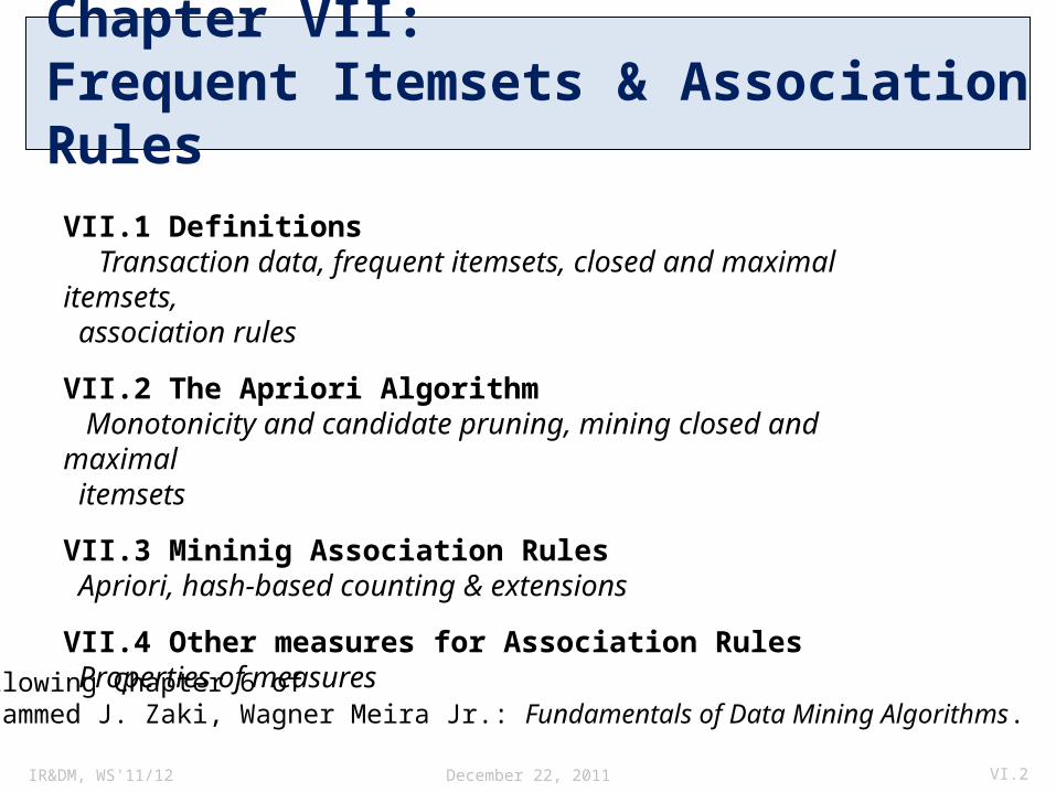
Lattice of items

VII.2 Apriori Algorithm for Mining Frequent Itemsets

IR&DM, WS'11/12

A Naïve Algorithm For Frequent Itemsets


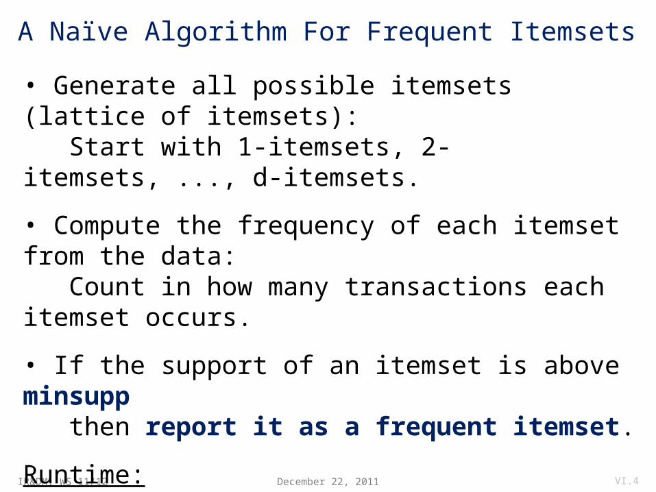
• Generate all possible itemsets (lattice of itemsets): Start with 1-itemsets, 2-itemsets, ..., d-itemsets.

• Compute the frequency of each itemset from the data: Count in how many transactions each itemset occurs.

• If the support of an itemset is above minsupp then report it as a frequent itemset.

Runtime:- Match every candidate against each transaction.- For M candidates and N=|D| transactions, the complexity is: O(N M) => this is very expensive since M = 2|I|

IR&DM, WS'11/12

Speeding Up the Naïve Algorithm


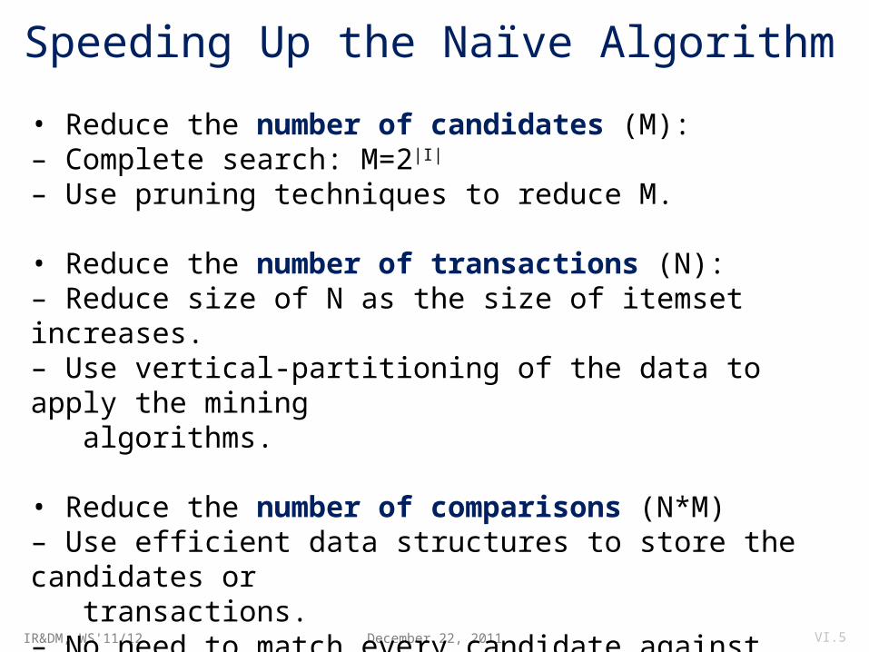
• Reduce the number of candidates (M):– Complete search: M=2|I|

– Use pruning techniques to reduce M.

• Reduce the number of transactions (N):– Reduce size of N as the size of itemset increases.– Use vertical-partitioning of the data to apply the mining algorithms.

• Reduce the number of comparisons (N*M)– Use efficient data structures to store the candidates or transactions.– No need to match every candidate against every transaction.

IR&DM, WS'11/12

Reducing the Number of Candidates


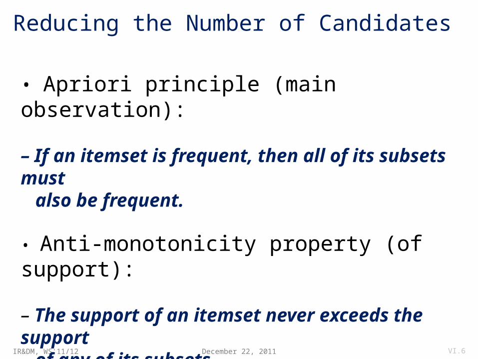
• Apriori principle (main observation):

– If an itemset is frequent, then all of its subsets must also be frequent.

• Anti-monotonicity property (of support):

– The support of an itemset never exceeds the support of any of its subsets.

IR&DM, WS'11/12

Apriori Algorithm: Idea and Outline

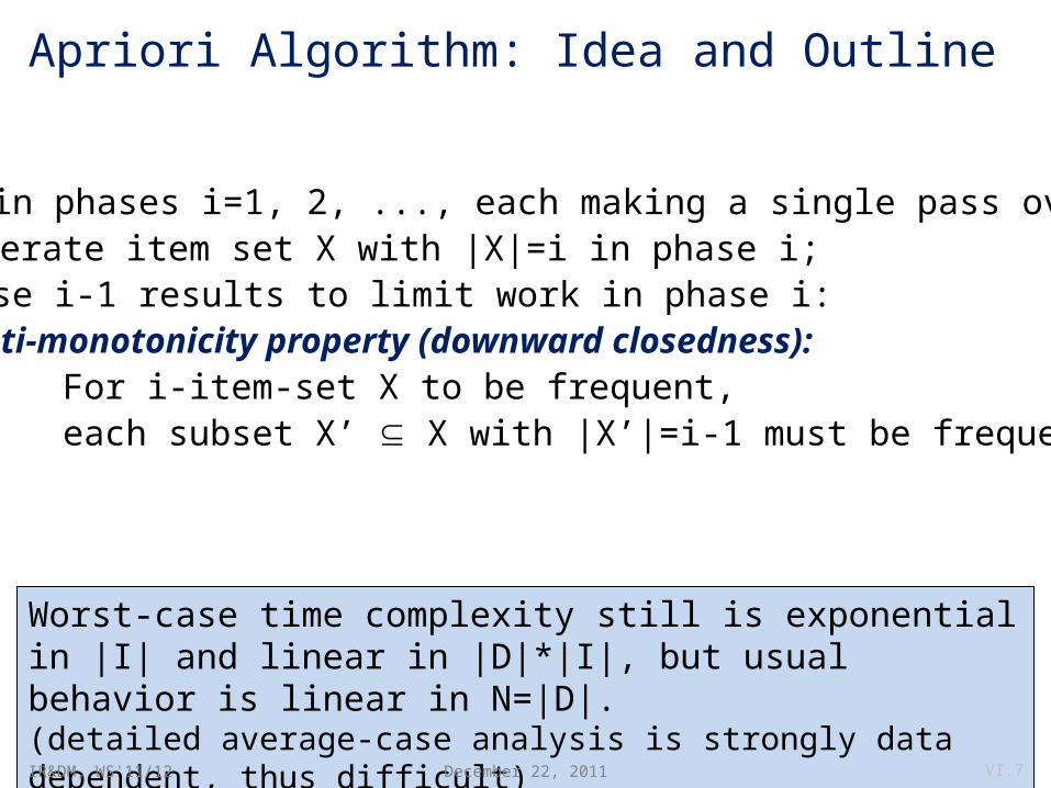
Outline:• Proceed in phases i=1, 2, ..., each making a single pass over D, and generate item set X with |X|=i in phase i;• Use phase i-1 results to limit work in phase i: Anti-monotonicity property (downward closedness): For i-item-set X to be frequent, each subset X’ X with |X’|=i-1 must be frequent, too;

Worst-case time complexity still is exponential in |I| and linear in |D|*|I|, but usual behavior is linear in N=|D|.(detailed average-case analysis is strongly data dependent, thus difficult)


IR&DM, WS'11/12

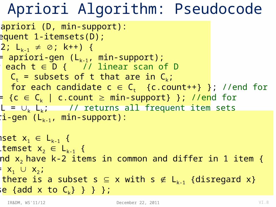
Apriori Algorithm: Pseudocodeprocedure apriori (D, min-support): L1 = frequent 1-itemsets(D); for (k=2; Lk-1 ; k++) { Ck = apriori-gen (Lk-1, min-support); for each t D { // linear scan of D Ct = subsets of t that are in Ck; for each candidate c Ct {c.count++} }; //end for Lk = {c Ck | c.count min-support} }; //end for return L = k Lk; // returns all frequent item setsprocedure apriori-gen (Lk-1, min-support): Ck = : for each itemset x1 Lk-1 { for each itemset x2 Lk-1 { if x1 and x2 have k-2 items in common and differ in 1 item { // join x = x1 x2; if there is a subset s x with s Lk-1 {disregard x} // infreq. subset else {add x to Ck} } } }; return Ck; December 22, 2011 VI.8

IR&DM, WS'11/12

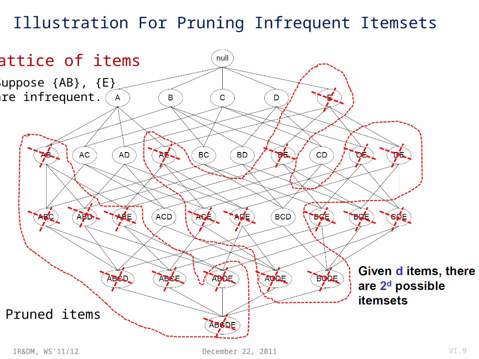
Illustration For Pruning Infrequent Itemsets


Suppose {AB}, {E}are infrequent.

Lattice of items

Pruned items

IR&DM, WS'11/12

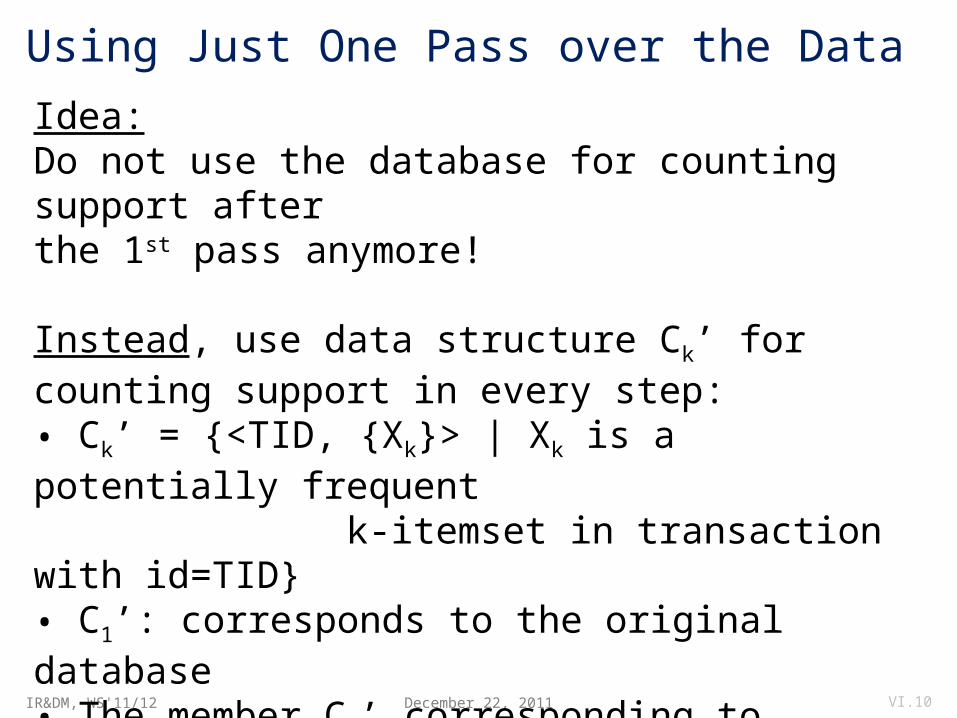
Using Just One Pass over the Data


Idea: Do not use the database for counting support after the 1st pass anymore!

Instead, use data structure Ck’ for counting support in every step:• Ck’ = {<TID, {Xk}> | Xk is a potentially frequent k-itemset in transaction with id=TID}• C1’: corresponds to the original database

• The member Ck’ corresponding to transaction t is defined as <t.TID, {c Ck | c is contained in t}>

IR&DM, WS'11/12

AprioriTID Algorithm: PseudoCode


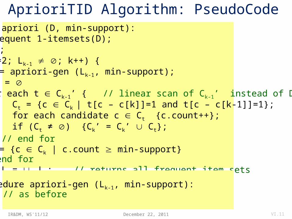
procedure apriori (D, min-support): L1 = frequent 1-itemsets(D); C1’ = D; for (k=2; Lk-1 ; k++) { Ck = apriori-gen (Lk-1, min-support); Ck’ = for each t Ck-1’ { // linear scan of Ck-1’ instead of D Ct = {c Ck | t[c – c[k]]=1 and t[c – c[k-1]]=1}; for each candidate c Ct {c.count++}; if (Ct ≠ ) {Ck’ = Ck’ Ct}; }; // end for Lk = {c Ck | c.count min-support} }; // end for return L = k Lk; // returns all frequent item sets

procedure apriori-gen (Lk-1, min-support): … // as before

IR&DM, WS'11/12

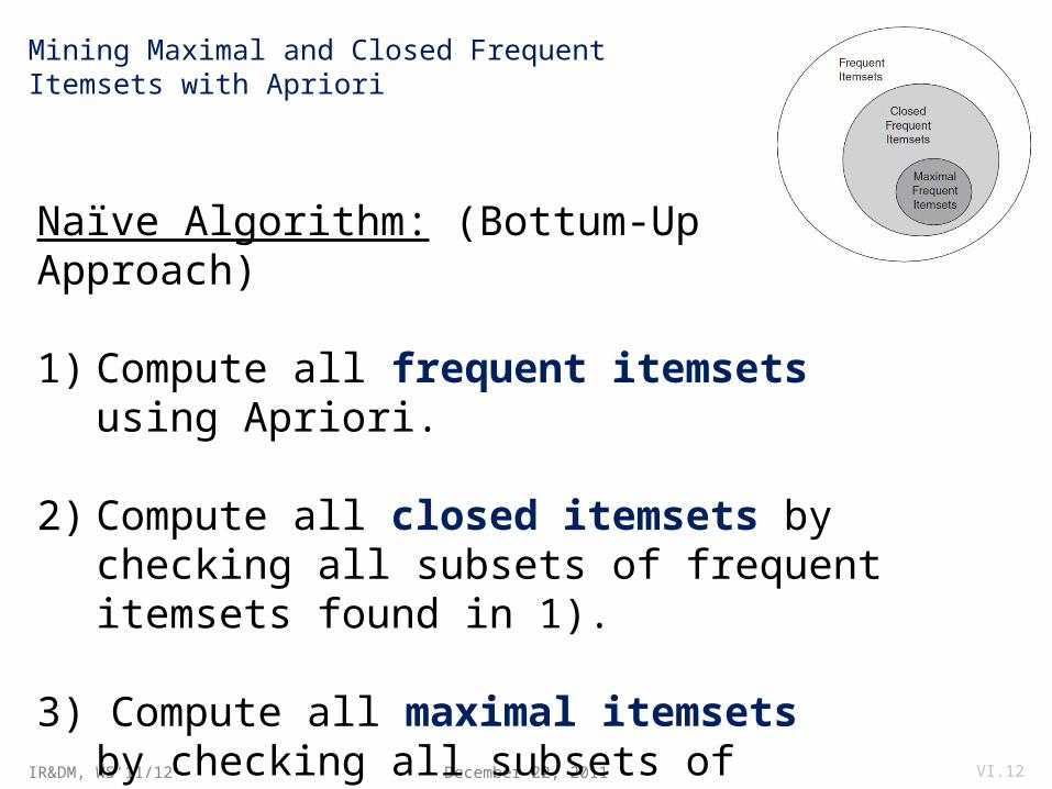
Mining Maximal and Closed Frequent Itemsets with Apriori


Naïve Algorithm: (Bottum-Up Approach)

1) Compute all frequent itemsets using Apriori.

2) Compute all closed itemsets by checking all subsets of frequent itemsets found in 1).

3) Compute all maximal itemsetsby checking all subsets of closed and frequent itemsets found in 2).

IR&DM, WS'11/12

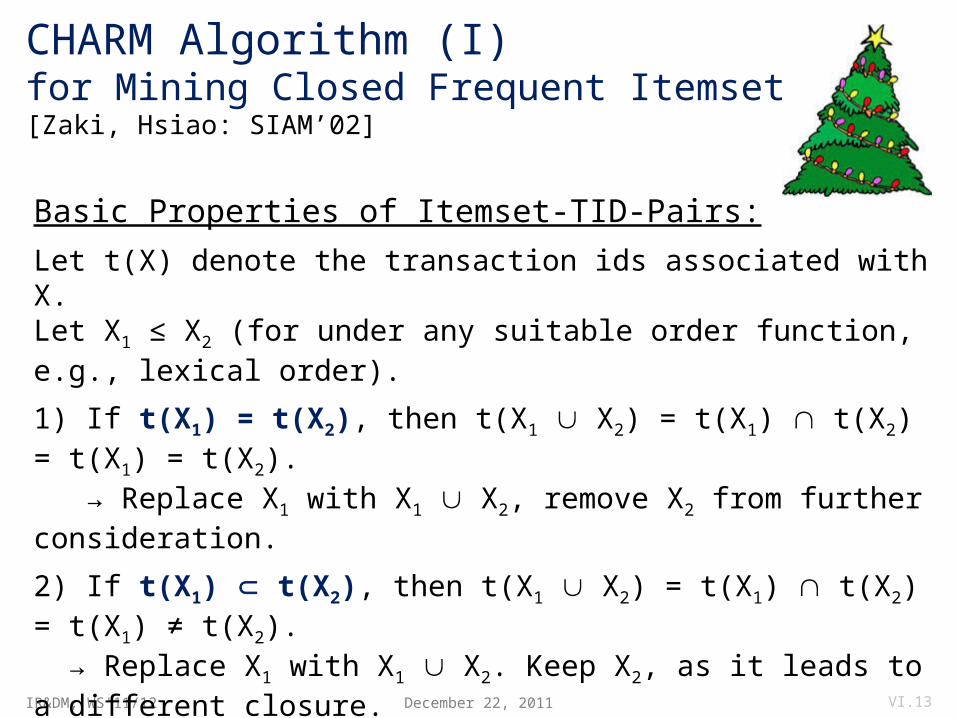
CHARM Algorithm (I)for Mining Closed Frequent Itemsets[Zaki, Hsiao: SIAM’02]


Basic Properties of Itemset-TID-Pairs:

Let t(X) denote the transaction ids associated with X.Let X1 ≤ X2 (for under any suitable order function, e.g., lexical order).

1) If t(X1) = t(X2), then t(X1 X2) = t(X1) t(X2) = t(X1) = t(X2). → Replace X1 with X1 X2, remove X2 from further consideration.

2) If t(X1) t(X2), then t(X1 X2) = t(X1) t(X2) = t(X1) ≠ t(X2). → Replace X1 with X1 X2. Keep X2, as it leads to a different closure.

3) If t(X1) t(X2), then t(X1 X2) = t(X1) t(X2) = t(X2) ≠ t(X1). → Replace X2 with X1 X2. Keep X1, as it leads to a different closure.

4) Else if t(X1) ≠ t(X2), then t(X1 X2) = t(X1) t(X2) ≠ t(X2) ≠ t(X1). → Do not replace any itemsets. Both X1 and X2 lead to different closures.

IR&DM, WS'11/12 December 22, 2011 VI.14

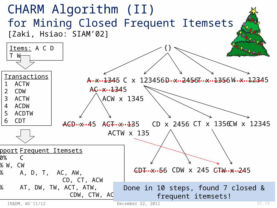
Items: A C D T W

Transactions1 ACTW2 CDW3 ACTW4 ACDW5 ACDTW6 CDT

Support Frequent Itemsets100% C84% W, CW67% A, D, T, AC, AW, CD, CT, ACW50% AT, DW, TW, ACT, ATW, CDW, CTW, ACTW

{}

A x 1345 C x 123456 D x 2456 T x 1356 W x 12345

AC x 1345ACW x 1345

ACD x 45 ACT x 135ACTW x 135

CD x 2456 CT x 1356 CW x 12345

CDT x 56 CDW x 245 CTW x 245

CHARM Algorithm (II)for Mining Closed Frequent Itemsets[Zaki, Hsiao: SIAM’02]

Done in 10 steps, found 7 closed & frequent itemsets!

IR&DM, WS'11/12

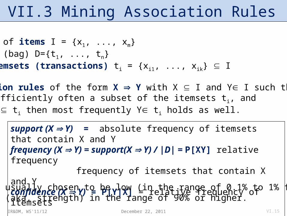
Given: • A set of items I = {x1, ..., xm}

• A set (bag) D={t1, ..., tn} of itemsets (transactions) ti = {xi1, ..., xik} IWanted: Association rules of the form X Y with X I and Y I such that • X is sufficiently often a subset of the itemsets ti, and• when X ti then most frequently Y ti holds as well.

support (X Y) = absolute frequency of itemsets that contain X and Yfrequency (X Y) = support(X Y) / |D| = P[XY] relative frequency

frequency of itemsets that contain X and Yconfidence (X Y) = P[Y|X] = relative frequency of itemsets that contain Y provided they contain X

Support is usually chosen to be low (in the range of 0.1% to 1% frequency),confidence (aka. strength) in the range of 90% or higher.

VII.3 Mining Association Rules


IR&DM, WS'11/12

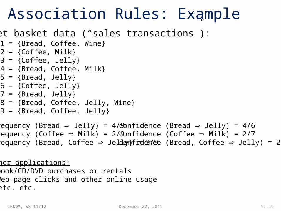
Association Rules: ExampleMarket basket data (“sales transactions”):

t1 = {Bread, Coffee, Wine}t2 = {Coffee, Milk}t3 = {Coffee, Jelly}t4 = {Bread, Coffee, Milk}t5 = {Bread, Jelly}t6 = {Coffee, Jelly}t7 = {Bread, Jelly}t8 = {Bread, Coffee, Jelly, Wine}t9 = {Bread, Coffee, Jelly}

frequency (Bread Jelly) = 4/9frequency (Coffee Milk) = 2/9frequency (Bread, Coffee Jelly) = 2/9

confidence (Bread Jelly) = 4/6confidence (Coffee Milk) = 2/7confidence (Bread, Coffee Jelly) = 2/4

Other applications:• book/CD/DVD purchases or rentals• Web-page clicks and other online usage etc. etc.


IR&DM, WS'11/12

Mining Association Rules with Apriori


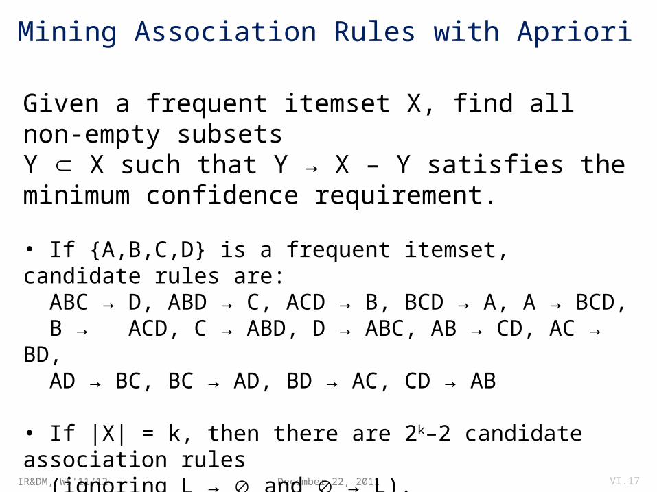
Given a frequent itemset X, find all non-empty subsets Y X such that Y → X – Y satisfies the minimum confidence requirement.

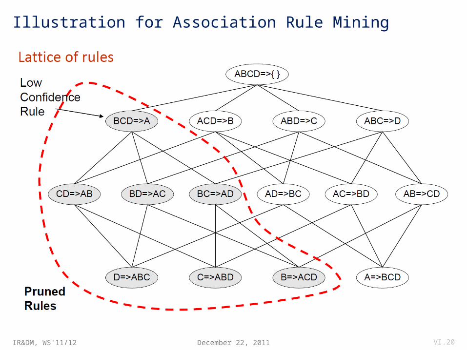
• If {A,B,C,D} is a frequent itemset, candidate rules are: ABC → D, ABD → C, ACD → B, BCD → A, A → BCD, B → ACD, C → ABD, D → ABC, AB → CD, AC → BD, AD → BC, BC → AD, BD → AC, CD → AB

• If |X| = k, then there are 2k–2 candidate association rules (ignoring L → and → L).

IR&DM, WS'11/12

Mining Association Rules with Apriori


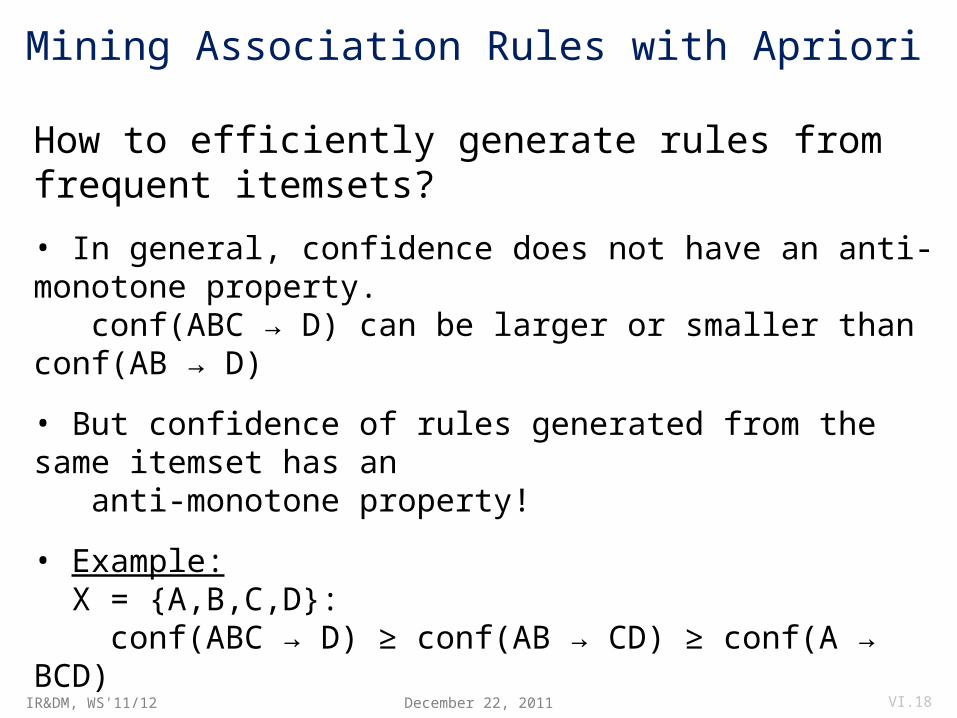
How to efficiently generate rules from frequent itemsets?

• In general, confidence does not have an anti-monotone property. conf(ABC → D) can be larger or smaller than conf(AB → D)

• But confidence of rules generated from the same itemset has an anti-monotone property!

• Example: X = {A,B,C,D}: conf(ABC → D) ≥ conf(AB → CD) ≥ conf(A → BCD)

Why? → Confidence is anti-monotone w.r.t. number of items on the RHS of the rule!

IR&DM, WS'11/12

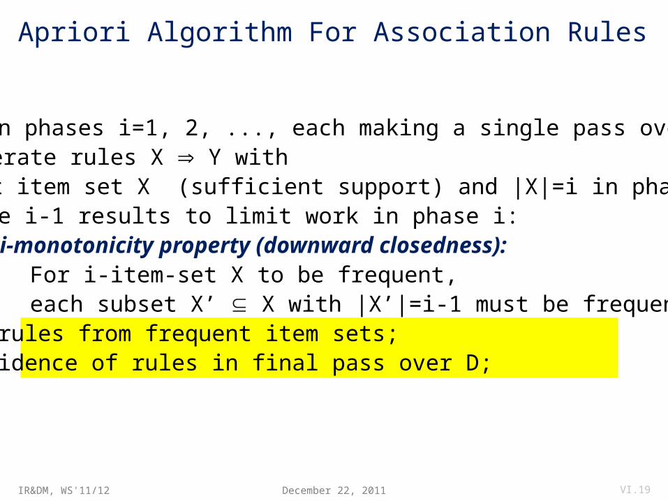
Apriori Algorithm For Association Rules

Outline:• Proceed in phases i=1, 2, ..., each making a single pass over D, and generate rules X Y with frequent item set X (sufficient support) and |X|=i in phase i;• Use phase i-1 results to limit work in phase i: Anti-monotonicity property (downward closedness): For i-item-set X to be frequent, each subset X’ X with |X’|=i-1 must be frequent, too;• Generate rules from frequent item sets;• Test confidence of rules in final pass over D;


IR&DM, WS'11/12

Illustration for Association Rule Mining


IR&DM, WS'11/12

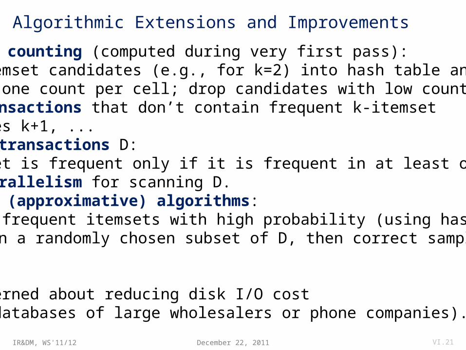
Algorithmic Extensions and Improvements• Hash-based counting (computed during very first pass): map k-itemset candidates (e.g., for k=2) into hash table and maintain one count per cell; drop candidates with low count early.• Remove transactions that don’t contain frequent k-itemset for phases k+1, ...• Partition transactions D: An itemset is frequent only if it is frequent in at least one partition.• Exploit parallelism for scanning D.• Randomized (approximative) algorithms: Find all frequent itemsets with high probability (using hashing, etc.).• Sampling on a randomly chosen subset of D, then correct sample....

Mostly concerned about reducing disk I/O cost(for TByte databases of large wholesalers or phone companies).


IR&DM, WS'11/12

Hash-based Counting of Itemsets


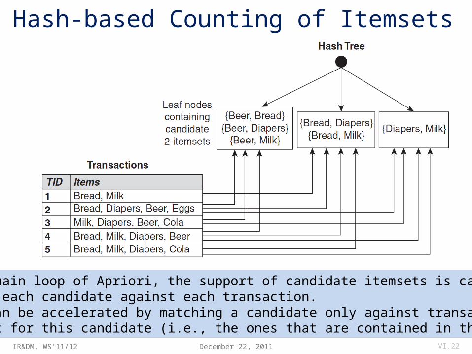
• During the main loop of Apriori, the support of candidate itemsets is calculated by matching each candidate against each transaction.• This step can be accelerated by matching a candidate only against transactions that are relevant for this candidate (i.e., the ones that are contained in the same bucket).

IR&DM, WS'11/12

Hash-Tree Index for Itemsets


1 4 5

1 2 44 5 7

1 2 54 5 8

1 5 9

1 3 6

2 3 45 6 7

3 4 53 5 63 5 76 8 9

3 6 73 6 8

H

H

H

H

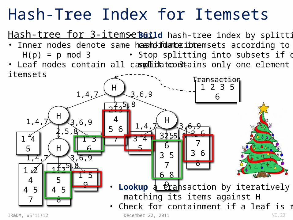
Hash-tree for 3-itemsets:• Inner nodes denote same hash-function H(p) = p mod 3• Leaf nodes contain all candidate 3-itemsets

1,4,7

2,5,8

3,6,9 1 2 3 5 6

Transaction

• Build hash-tree index by splitting candidate itemsets according to H • Stop splitting into subsets if current split contains only one element

1,4,72,5,8

3,6,9 1,4,72,5,8

3,6,9

1,4,72,5,8

3,6,9

• Lookup a transaction by iteratively matching its items against H• Check for containment if a leaf is reached

IR&DM, WS'11/12

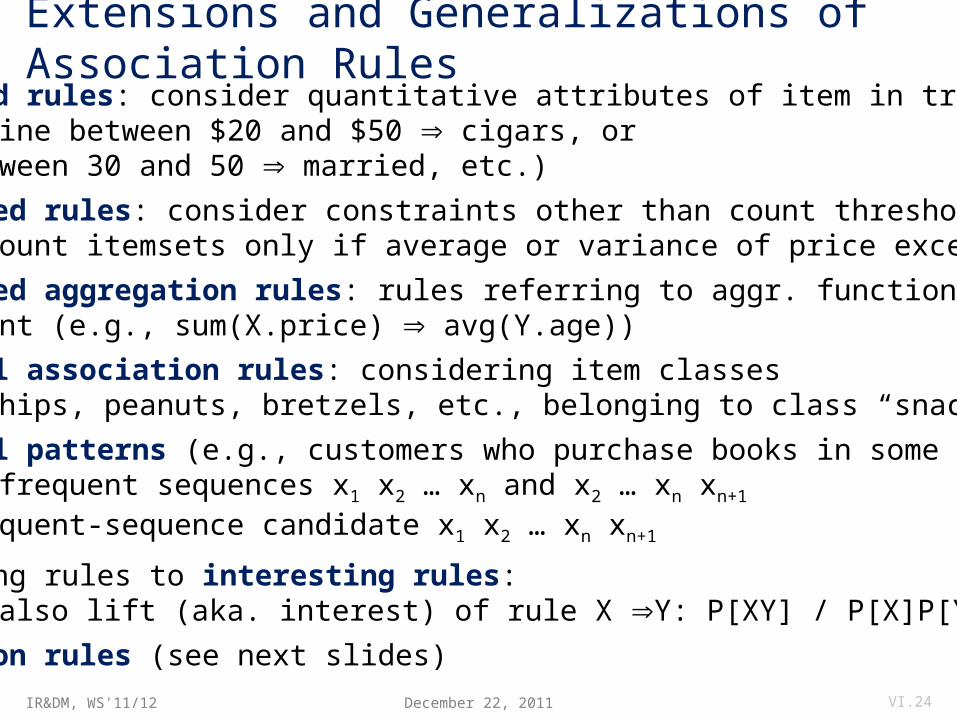
Extensions and Generalizations of Association Rules• Quantified rules: consider quantitative attributes of item in transactions (e.g., wine between $20 and $50 cigars, or age between 30 and 50 married, etc.)• Constrained rules: consider constraints other than count thresholds, (e.g., count itemsets only if average or variance of price exceeds ...)• Generalized aggregation rules: rules referring to aggr. functions other than count (e.g., sum(X.price) avg(Y.age))• Multilevel association rules: considering item classes (e.g., chips, peanuts, bretzels, etc., belonging to class “snacks”)• Sequential patterns (e.g., customers who purchase books in some order): combine frequent sequences x1 x2 … xn and x2 … xn xn+1

into frequent-sequence candidate x1 x2 … xn xn+1

• From strong rules to interesting rules: consider also lift (aka. interest) of rule X Y: P[XY] / P[X]P[Y]• Correlation rules (see next slides)


IR&DM, WS'11/12

VII.4 Other Measures For Association Rule Mining


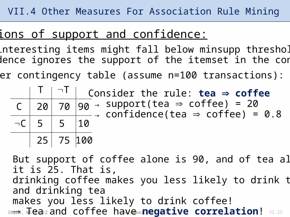
Limitations of support and confidence:(a) Many interesting items might fall below minsupp threshold!(b) Confidence ignores the support of the itemset in the consequent!

Consider the rule: tea coffee → support(tea coffee) = 20 → confidence(tea coffee) = 0.8

Consider contingency table (assume n=100 transactions):

But support of coffee alone is 90, and of tea alone it is 25. That is,drinking coffee makes you less likely to drink tea, and drinking teamakes you less likely to drink coffee! Tea and coffee have negative correlation!

C

T T

C

20 70 90

1055

25 75 100

IR&DM, WS'11/12

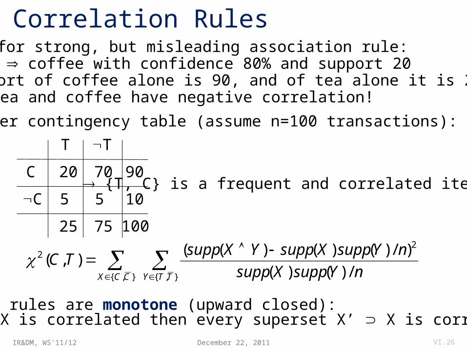
Correlation RulesExample for strong, but misleading association rule: tea coffee with confidence 80% and support 20But support of coffee alone is 90, and of tea alone it is 25 tea and coffee have negative correlation!


Correlation rules are monotone (upward closed):If the set X is correlated then every superset X’ X is correlated, too.

{T, C} is a frequent and correlated item set

},{ },{

22

/)()(

)/)()()((),(

CCX TTY nYsuppXsupp

nYsuppXsuppYXsuppTC


C

T T

C

20 70 90

1055

25 75 100

IR&DM, WS'11/12

Correlation Rules

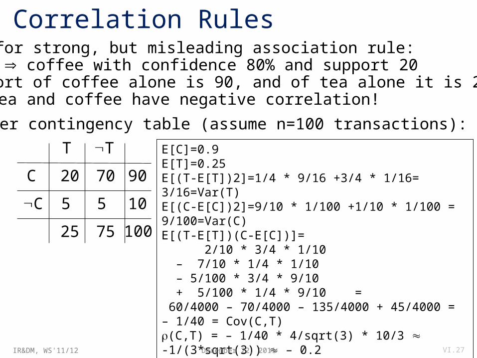
E[C]=0.9E[T]=0.25E[(T-E[T])2]=1/4 * 9/16 +3/4 * 1/16= 3/16=Var(T)E[(C-E[C])2]=9/10 * 1/100 +1/10 * 1/100 = 9/100=Var(C)E[(T-E[T])(C-E[C])]= 2/10 * 3/4 * 1/10 – 7/10 * 1/4 * 1/10 – 5/100 * 3/4 * 9/10 + 5/100 * 1/4 * 9/10 = 60/4000 – 70/4000 – 135/4000 + 45/4000 = – 1/40 = Cov(C,T)(C,T) = – 1/40 * 4/sqrt(3) * 10/3 -1/(3*sqrt(3)) – 0.2

Example for strong, but misleading association rule: tea coffee with confidence 80% and support 20But support of coffee alone is 90, and of tea alone it is 25 tea and coffee have negative correlation!



C

T T

C

20 70 90

1055

25 75 100

IR&DM, WS'11/12

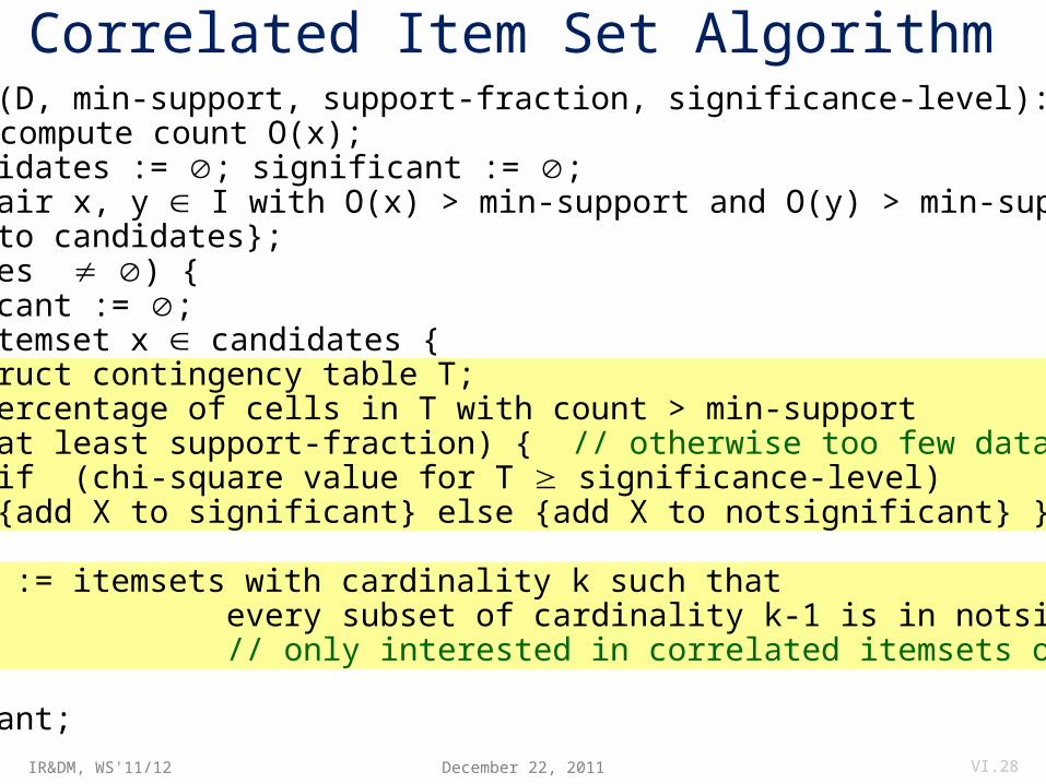
Correlated Item Set Algorithmprocedure corrset (D, min-support, support-fraction, significance-level): for each x I compute count O(x); initialize candidates := ; significant := ; for each item pair x, y I with O(x) > min-support and O(y) > min-support { add (x,y) to candidates}; while (candidates ) { notsignificant := ; for each itemset x candidates { construct contingency table T; if (percentage of cells in T with count > min-support is at least support-fraction) { // otherwise too few data for chi-square if (chi-square value for T significance-level) {add X to significant} else {add X to notsignificant} } }; // if/for

candidates := itemsets with cardinality k such that every subset of cardinality k-1 is in notsignificant; // only interested in correlated itemsets of min. cardinality }; //while return significant;


IR&DM, WS'11/12

Examples of Contingency Tables


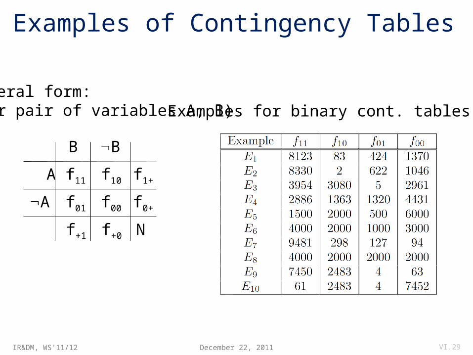
A

B B

A

f11 f10 f1+

f0+f00f01

f+1 f+0

General form: (for pair of variables A, B)

N

Examples for binary cont. tables:

IR&DM, WS'11/12

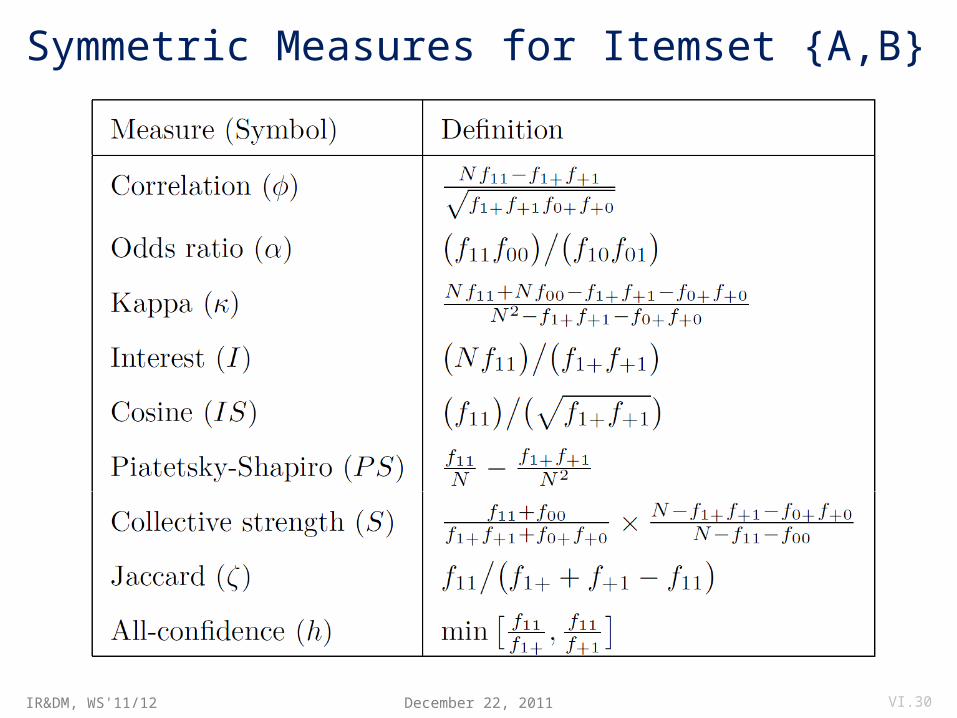
Symmetric Measures for Itemset {A,B}


IR&DM, WS'11/12

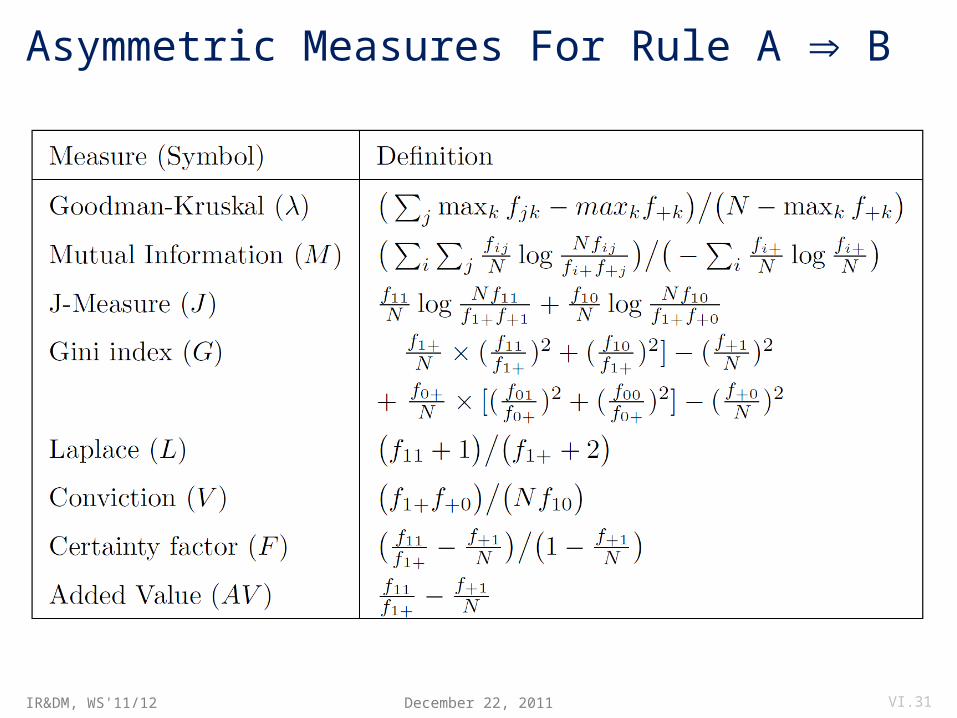
Asymmetric Measures For Rule A B


IR&DM, WS'11/12

Consistency of Measures


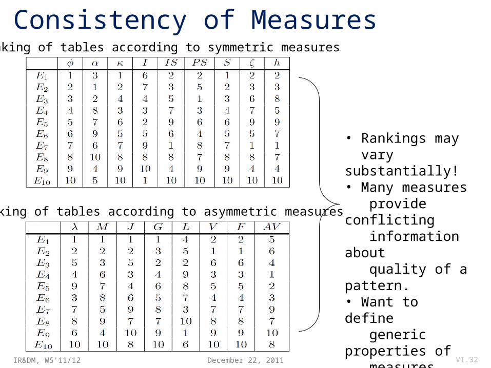
Ranking of tables according to symmetric measures

Ranking of tables according to asymmetric measures

• Rankings may vary substantially!• Many measures provide conflicting information about quality of a pattern.• Want to define generic properties of measures.

IR&DM, WS'11/12

Properties of Measures


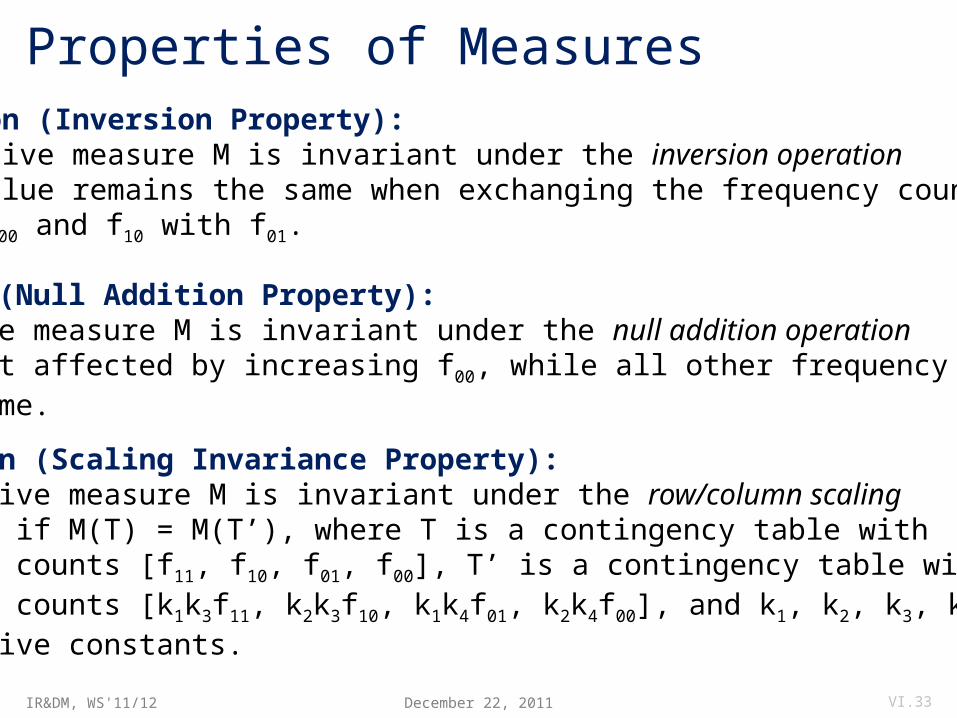
Definition (Inversion Property):An objective measure M is invariant under the inversion operationif its value remains the same when exchanging the frequency counts f11 with f00 and f10 with f01.

Definition (Null Addition Property):An objective measure M is invariant under the null addition operationif it is not affected by increasing f00, while all other frequency countsstay the same.

Definition (Scaling Invariance Property):An objective measure M is invariant under the row/column scalingoperation if M(T) = M(T’), where T is a contingency table with frequency counts [f11, f10, f01, f00], T’ is a contingency table with frequency counts [k1k3f11, k2k3f10, k1k4f01, k2k4f00], and k1, k2, k3, k4

Are positive constants.

IR&DM, WS'11/12

Example: Confidence and the Inversion Property


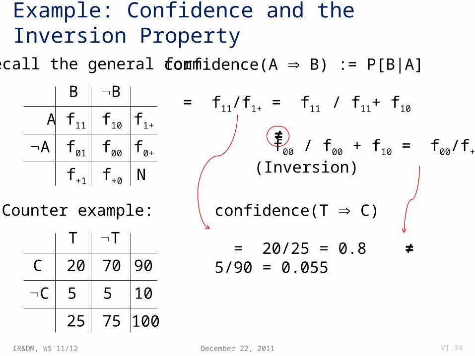
confidence(A B) := P[B|A]

= f11/f1+ = f11 / f11+ f10

f00 / f00 + f10 = f00/f+0

(Inversion)

A

B B

A

f11 f10 f1+

f0+f00f01

f+1 f+0 N

Counter example:

C

T T

C

20 70 90

1055

25 75

Recall the general form:

confidence(T C)

= 20/25 = 0.8 ≠ 5/90 = 0.055

≠

100

IR&DM, WS'11/12

Simpson’s Paradox (I)


H

E E

H

99 81 180

1206654

153 147 300

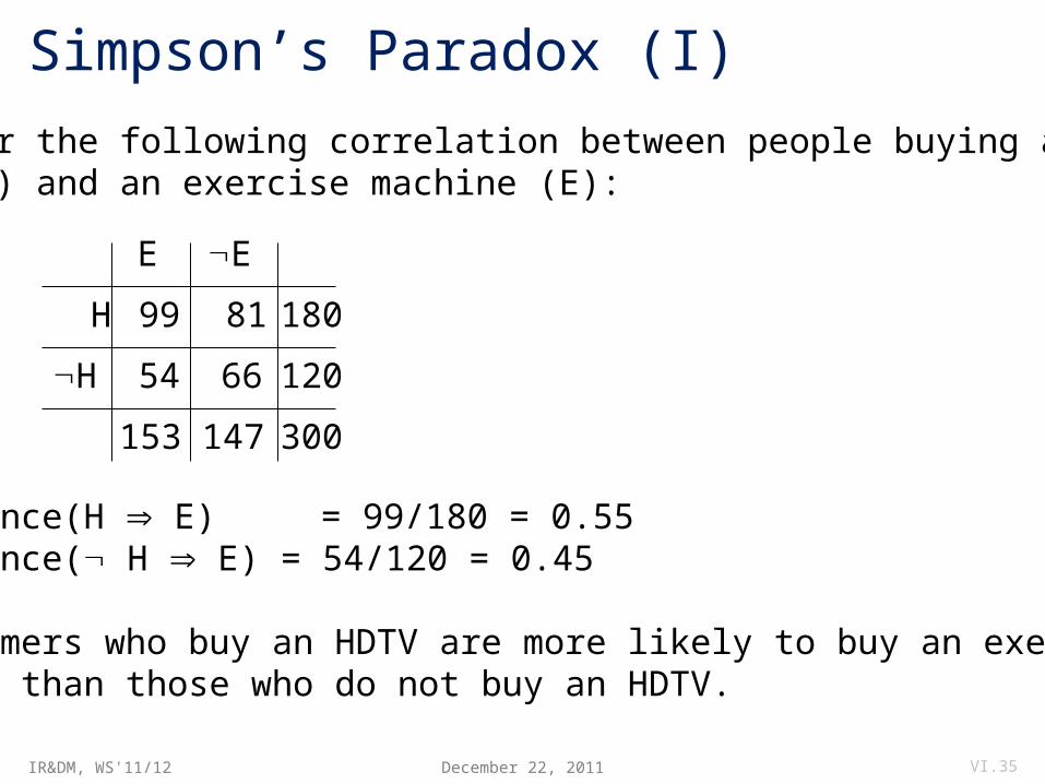
Consider the following correlation between people buying anHTDV (H) and an exercise machine (E):

confidence(H E) = 99/180 = 0.55confidence( H E) = 54/120 = 0.45

→ Customers who buy an HDTV are more likely to buy an exercise machine than those who do not buy an HDTV.

IR&DM, WS'11/12

Simpson’s Paradox (II)


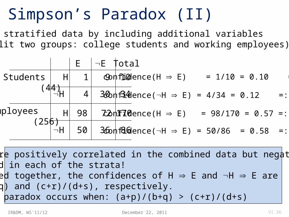
Consider stratified data by including additional variables(data split two groups: college students and working employees):

confidence(H E) = 1/10 = 0.10 =: a/b

confidence(H E) = 4/34 = 0.12 =: c/d

confidence(H E) = 98/170 = 0.57 =: p/q

confidence(H E) = 50/86 = 0.58 =: r/s

H

E E

H

1 9 10

34304

H

H

98 72 170

863650

Total

Students (44)

Employees (256)

H and E are positively correlated in the combined data but negativelycorrelated in each of the strata!When pooled together, the confidences of H E and H E are (a+p)/(b+q) and (c+r)/(d+s), respectively.Simpson’s paradox occurs when: (a+p)/(b+q) > (c+r)/(d+s)

IR&DM, WS'11/12

Summary of Section VII


Mining frequent itemset and association rules is a versatile tool for many applications (e-commerce, user recommendations, etc.).

One of the most basic building blocks in data mining for identifying interesting correlations among items/objects based on co-occurrence statistics.

Complexity issues mostly due to the huge amount of possible combinations of candidate itemsets (and rules), also expensive when amount of transactions is huge and needs to be read from disk.

Apriori builds on anti-monotonicity property of support, whereas confidence does not generally have this property (however pruning is possible to some extent within a given itemset).

Many quality measures considered in the literature, each with different properties.

Additional Literature:M. J. Zaki and C. Hsiao: CHARM: An efficient algorithm for closed itemset mining. SIAM’02.

Documents

Chapter VII: Frequent Itemsets & Association Rules