Embed Size (px)
Citation preview
Art. 1.] INTRODUCTION. 467
Chapter X.
PROBABILITY AND THEORY OF ERRORS.
By Robert S. Woodward,Professor of Mechanics in Columbia University.
Art. 1. Introduction.
It is a curious circumstance that a science so profoundly
mathematical as the theory of probability should have origi-
nated in the games of chance which occupy the thoughtless
and profligate.* That such is the case is sufficiently attested
by the fact that much of the terminology of the science and
many of its familiar illustrations are drawn directly from the
vocabulary and the paraphernalia of the gambler and the trick-
ster. It is somewhat surprising, also, considering the antiquity
of games of chance, that formal reasoning on the simpler
questions in probability did not begin before the time of Pascal
and Fermat. Pascal was led to consider the subject during the
year 1654 through a problem proposed to him by the Chevalier
de Mere, a reputed gambler.f The problem in question is
known as the problem of points and may be stated as follows
:
two players need each a given number of points to win at a
certain stage of their game ; if they stop at this stage, how should
the stakes be divided ? Pascal corresponded with his friend
Fermat on this question ; and it appears that the letters which
passed between them contained the earliest distinct formulation
of principles falling within the theory of probability. These
* The historical facts referred to in this article are drawn mostly from Tod-
hunter's History of the Mathematical Theory of Probability from the time of
Pascal to that of Laplace (Cambridge and London, 1865).
t" Un probleme relatif aux jeux de hasard, propose^ aun austere janseniste
par un homme du monde, a et6 l'origine du calcul des probabilitfes.'' Poisson,
Recherches surla Probability des Jugements (Paris, 1837).

468 PROBABILITY AND THEORY OF ERRORS. [Chap. X
acute thinkers, however, accomplished little more than a correct
start in the science. Each seemed to rest content at the time-
with the approbation of the other. Pascal soon renounced
such mundane studies altogether ; Fermat had only the scant
leisure of a life busy with affairs to devote to mathematics;
and both died soon after the epoch in question,—Pascal in
1662, and Fermat in 1665.
A subject which had attracted the attention of such dis-
tinguished mathematicians could not fail to excite the interest
of their contemporaries and successors. Amongst the former
Huygens is the most noted. He has the honor of publishing
the first treatise* on the subject. It contains only fourteen
propositions and is devoted entirely to games of chance, but it
gave the best account of the theory down to the beginning of
the eighteenth century, when it was superseded by the more elab-
orate works of James Bernoulli,f Montmort,^: and De Moivre.§
Through the labors of the latter authors the mathematical
theory of probability was greatly extended. They attacked,
quite successfully in the main, the most difficult problems;
and great credit is due them for the energy and ability dis-
played in developing a science which seemed at the time to-
have no higher aim than intellectual diversion. | Their names,,
undoubtedly, with one exception, that of Laplace, are the most
important in the history of probability.
Since the beginning of the eighteenth century almost every
mathematician of note has been a contributor to or an expos-
itor of the theory of probability. Nicolas, Daniel, and John
Bernoulli, Simpson, Euler, dAlembert, Bayes, Lagrange, Lam-
bert, Condorcet, and Laplace are the principal names which
figure in the history of the subject during the hundred years
*De Ratiociniis in Ludo Aleae, 1657.
fArs Conjectandi, 1713.
JEssai d'Analyse sur les Jeux de Hazards, 1708.
§ The Doctrine of Chances, 1718.
I!
Todhunter says of Montmort, for example, " In 1708 he published his
work on Chances, where with the courage of Columbus he revealed a new world,
to Mathematicians."
Art. 1.] INTRODUCTION. 469
ending with the first quarter of the present century. Of the
contributions from this brilliant array of mathematical talent,
the Th6orie Analytique des Probabilites of Laplace is by far
the most profound and comprehensive. It is, like his Me-canique Celeste in dynamical astronomy, still the most elabo-
rate treatise on the subject. An idea of the grand scale of the
work in its present form* maybe gained by the facts that the
non-mathematical introduction! covers about one hundred and
fifty quarto pages ; and that, in spite of the extraordinary
brevity of mathematical language, the pure theory and its ac-
cessories and applications require about six hundred and fifty
pages.
From the epoch of Laplace down to the present time the
extensions of the science have been most noteworthy in the
fields of practical applications, as in the adjustment of obser-
vations, and in problems of insurance, statistics, etc. Amongstthe most important of the pioneers in these fields should
be mentioned Poisson, Gauss, Bessel, and De Morgan. Nu-
merous authors, also, have done much to simplify one or an-
other branch of the subject and thus bring it within the range
of elementary presentation. The fundamental principles of
the theory are, indeed, now accessible in the best text-books
on algebra : and there are many excellent treatises on the pure
theory and its various applications.
Of all the applications of the doctrine of probability none
is of greater utility than the theory of errors. In astronomy,
geodesy, physics, and chemistry, as in every science which at-
tains precision in measuring, weighing, and computing, a
knowledge of the theory of errors is indispensable. By the aid
of this theory the exact sciences have made great progress dur-
*The form of the third edition published in 1820, and of Vol. VII of the
complete works of Laplace recently republished under the auspices of the
Academie des Sciences by Gauthier-Villars. This Vol. VII bears the date 1886.
f" Cette Introduction," writes Laplace, "est le developpement d'une Lecon
sur les Probabilites, que je donnai en 1795, aux Ecoles Normales, ou je fus ap-
pele comme professeur de Mathematiques avec Lagrange, par un decret de la
Convention nationale."
470 PROBABILITY AND THEORY OF ERRORS. [Chap. X.
ing the present century, not only in the actual determination
of the constants of nature, but also in the fixation of clear
ideas as to the possibilities of future conquests in the same di-
rection. Nothing, for example, is more satisfactory and in-
structive in the history of science than the success with which
the unique method of least squares has been applied to the
problems presented by the earth and the other members of the
solar system. So great, in fact, are the practical value and
theoretical importance of the method of least squares, that it is
frequently mistaken for the whole theory of errors, and is
sometimes regarded as embodying the major part of the doc-
trine of probability itself.
As may be inferred from this brief sketch, the theory of
probability and its more important applications now constitute
an extensive body of mathematical principles and precepts.
Obviously, therefore, it will be impossible within the limits of
a single chapter of this volume to do more than give an out-
line of the salient features of the subject. It is hoped, how-
ever, in accordance with the general plan of the volume, that
such outline will prove suggestive and helpful to those who'
may come to the science for the first time, and also to those
who, while somewhat familiar with the difficulties to be over-
tome, have not acquired a working knowledge of the subject.
Effort has been made especially to clear up the difficulties of
the theory of errors by presenting a somewhat broader view of
the elements of the subject than is found in the standard
treatises, which confine attention almost exclusively to the
method of least squares. This chapter stops short of that
method, and seeks to supply those phases of the theory which
are either notably lacking or notably erroneous in works
hitherto published. It is believed, also, that the elements here
presented are essential to an adequate understanding of the
well-worked domain of least squares.*
*The auihor has given a brief but comprehensive statement of the method
of least squares in the volume of Geographical Tables published by the Smith-
sonion Institution, 1894.
Art. 2.] permutations. 471
Art. 2. Permutations.
The formulas and results of the theory of permutationsand combinations are often needed for the statement and so-
lution of problems in probabilities. This theory is now to befound in most works on algebra, and it will therefore suffice
here to state the principal formulas and illustrate their mean-ing by a few numerical examples.
The number of permutations of n things taken r in a groupis expressed by the formula
(n) r = n{n — i)(« - 2) ...(«- r + i). (i)
Thus, to illustrate, the number of ways the four letters a, b,
c, d can be arranged in groups of two is 4 . 3 = 1 2, and the groupsare
ab, ba, ac, ca, ad, da, be, cb, bd, db, cd, dc.
Similarly, the formula gives for
n = 3 and r = 2, (3), = 3.2 = 6,
n= 7 " r = 3, (7)3 = 7-6.5 =210,n — 10 " r = 6, (10), = 10.9.8.7.6. 5 = 151200.
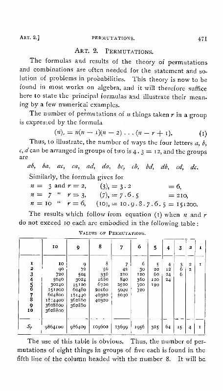
The results which follow from equation (1) when n and r
do not exceed 10 each are embodied in the following table :
Values of Permutations.
472 PROBABILITY AND THEORY OF ERRORS. [Chap. X.
noticed that the last two numbers in each column (excepting
that headed with i) are the same. This accords with the for-
mula, which gives for the number of permutations of n things
in groups of n the same value as for n things in groups of
(n — i). It will also be remarked that the last number in each
column of the table is the factorial, n\, of the number n at the
head of the column. For example, in the column under 7, the
last number is 5040 = 1.2.3.4.5.6.7 = 7!.
The total number of permutations of n things taken singly,
in groups of two, three, etc., is found by summing the numbers
given by equation (1) for all values of r from 1 to «.. Calling
this total or sum Sp , it will be given by
St = Z(n\. (2)
To illustrate, suppose n = 3, and, to fix the ideas, let the
three things be the three digits 1, 2, 3. Then from the above
table it is seen that St = 3 + 6 -\- 6 = 15 ; or, that the number
of numbers (all different) which can be formed from those dig-
its is fifteen. These numbers are 1, 2, 3 ; 12, 13, 21, 23, 31, 32;
123, 132, 213, 231, 312, 321.
The values of St for n = 1, 2, ... 10 are given under the
corresponding columns of the above table. But when n is
large the direct summation indicated by (2) is tedious, if not
impracticable. Hence a more convenient formula is desirable.
To get this, observe that (1) may be written
(^=(^)!' (I)'
if r is restricted to integer values between 1 and (n — 1), both
inclusive. This suffices to give all terms which appear in the
right-hand member of (2), since the number of permutations
for r — (n — 1) is the same as for r = n. Hence it appears
that
St —n\-\--1 ^1.2^' ••{n - l)\
.Art. 3.] combinations. 473
But as n increases, the series by which n ! is here multiplied
approximates rapidly towards the base of natural logarithms
;
that is, towards
* = 2.7182818 -h log e = 0.4342945.
Hence for large values of n
Sp = n\e, approximately.* (3)
To get an idea of the degree of approximation of (3), sup-
pose n = 9. Then the computation runs thus (see values in
the above table)
:
log
91 = 362880 5-5597630
e 0.4342945
9!* = 986410 5-9940575
Sp = 986409 by equation (2).
The error in this case is thus seen to be only one unit, or
about one-millionth of Sp.j-
Prob. 1. Tabulate a list of the numbers of three figures each
which can be formed from the first five digits 1, . . . 5. How manynumbers can be formed from the nine digits ?
Prob. 2. Is Sj, always an odd number for n odd ? Observevalues of Sp in the table above.
Art. 3. Combinations.
In permutations attention is given to the order of arrange-
ment of the things considered. In combinations no regard is
paid to the order of arrangement. Thus, the permutations of
the letters a, b, c, d in groups of three are
(abc) (abd) bac bad acb {acd) cab cad
adb adc dab dac bca {bed) cba cbd
bda bde dba dbc cda cdb dca deb
* See Art. 6 for a formula for computing »! when n is a large number.
f When large numbers are to be dealt with, equations (1)' and (3) are easily
managed by logarithms, especially if a table of values of log («!) is available.
Such tables are given to six places in De Morgan's treatise on Probability in
the Encyclopaedia Metropolitana, and to five places in Shortrede's Tables
{Vol. I, 1849).
474 PROBABILITY AND THEORY OF ERRORS. [Chap. X.
But if the order of arrangement is ignored all of these are
seen to be repetitions of the groups enclosed in parentheses,
namely, {abc), (add), (acd), (bed). Hence in this case out of
twenty-four permutations there are only four combinations.
A general formula for computing the number of combina-
tions of n things taken in groups of r things is easily derived.
For the number of permutations of n things in groups of r is
by (i) of Art. 2
(n) r = n(n — i)(n — 2) ...(« — r -f- 1)
;
and since each group of r things gives 1.2.3.. f — rl per-
mutations, the number of combinations must be the quotient
of («)r by r\. Denote this number by C(n) r. Then the gen-
eral formula is
»(»- i)(»-2)...(»-r+i)4")r = y\ W
This formula gives, for example, in the case of the four let-
ters a, b, c, d taken in groups of three, as considered above,
4.3.2
Multiply both numerator and denominator of the right-hand
member of (1) by (n — r)\ The result is
n\ , ,
,
v ,r r\ (n — r) !
which shows that the number of combinations of n things in
groups of r is the same as the number of combinations of n
things in groups of (« — r). Thus, the number of combina-
tions of the first ten letters a, b, c . . J in groups of three or
seven is
10!—:—: = 120.3 '• 7 1
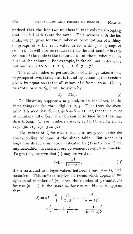
The following table gives the values C(n) r for all values of
n and r from 1 to 10.
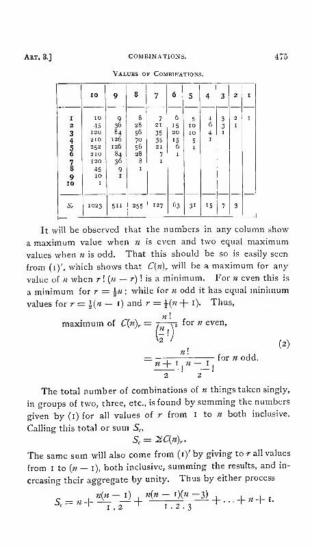
The mode of using this table is evident. For example, the
number of combinations of eight things in sets of five each is
found on the fifth line of the column headed 8 to be 56.
Art. 3.] combinations.
Values of Combinations.
475
476 PROBABILITY AND THEORY OF ERRORS. [CHAP. X.
The second member of this equation is evidently equal to
(i 4- i)" — I. Hence
Sc= 2C(n) r = 2" - r.
( 3 )
The values of Scfor values of n and r from i to io are given
under the corresponding columns of the above table.
Prob. 3. How many different squads of ten men each can be
formed from a company of 100 men ?
Prob. 4 How many triangles are formed by six straight lines
each of which intersects the other five ?
Prob. 5. Examine this statement :" In dealing a pack of cards
the number of hands, of thirteen cards each, which can be produced
is 635 013 559 600. But in whist four hands are simultaneously held,
and the number of distinct deals . . . would require twenty-eight
figures to express it."*
Prob. 6. Assuming combination always possible, and disregarding
the question of proportions, find how many different substances
could be produced by combining the seventy-three chemical ele-
ments.
Art. 4. Direct Probabilities.
If it is known that one of two events must occur in any
trial or instance, and that the first can occur in a ways and the
second in b ways, all of which ways are equally likely to hap-
pen, then the probability that the first will happen is expressed
mathematically by the fraction a/(a-\-b), while the probability
that the second will happen is b/(a-\-b). Such events are said
to be mutually exclusive. Denote their probabilities by/ and
q respectively. Then there result
the last equation following from the first two and being the
mathematical expression for the certainty that one of the two
events must happen.
Thus, to illustrate, in tossing a coin it must give " head " or
" tail" ; a = b = 1, and p = q = 1/2. Again, if an urn contain
.a = 5 white and 3 = 8 black balls, the probability of drawing
* Jevons, Principles of Science, p. 217.
Art. 4.] direct probabilities. 477
a white ball in one trial is p = 5/13 and that of drawing a.
black one q = 8/13.
Similarly, if there are several mutually exclusive events
which can occur in a, b, c. . . ways respectively, their probabil-
ities/, q, r . . . are given by
a b c
P = a+b+c-\-. -•'
q = a -\-b+c-\-. ..
'
r =a -\-b+c-\-. ..
'
(2):
P + 9+ r + -- • = I-
For example, if an urn contain a = 4 white, b = 5 black,,
and c = 6 red balls, the probabilities of drawing a white, black,
and red ball at a single trial are ^ = 4/15, £=5/15, and.
y = 6/15, respectively.
Formulas (i) and (2) may be applied to a wide variety of
cases, but it must suffice here to give only a few such. As a
first illustration, consider the probability of drawing at random
a number of three figures from the entire list of numbers which
can be formed from the first seven digits. A glance at the
table of Art. 1 shows that the symbols of formula (1) have in.
this case the values a= 210, and a-\-b= 13699. Hence
b = 13489, and p = 2 10/13699 ; that is, the probability in ques-
tion is about 1/65.
Secondly, what is the probability of holding in a hand of
whist all the cards of one suit ? Formula (1) of Art. 3 shows
that the number of different hands of thirteen cards each which
may be formed from a pack of fifty-two cards is
52. 51.50. . .40 . ,
^ 1 !L_ —635013 559600,I . 2 .3 ... 13 ^ °
DDV
and the probability required is the reciprocal of this number.
The probability against this event is, therefore, very nearly
unity.
Thirdly, consider the probabilities presented by the case of
an urn containing 4 white, 5 black, and 6 red balls, from which
at a single trial three balls are to be drawn. Evidently the
triad of balls drawn may be all white, all black, all red, partly
white and black, partly white and red, partly black and red, or
I
Art. 5.] PROBABILITY OF CONCURRENT EVENTS. 479
Art. 5. Probability of Concurrent Events.
If the probabilities of two independent events are/, and
/„ respectively, the probability of their concurrence in anysingle instance is pj>v Thus, suppose there are two urns
C/j and Uv the first of which contains «, white and b1black
balls, and the second atwhite and b, black balls. Then the
probability of drawing a white ball from U1is/, = «,/(«, + £,),
while that of drawing a white ball from cT, isA = a,/(aa-\- b,).
The total number of different pairs of balls which can be formed
from the entire number of balls is («, + £,)(«, + b,). Of these
pairs «,«aare favorable to the concurrence of white in simul-
taneous or successive drawings from the two urns. Hence the
probability of a concurrence of
white with white = «,«,/(«, -(- <$,)(#2 + £,),
white with black = («A+ «A)/(«. + b,)(a% + &,),
black with black = bfij{ax -f- £,)(«, -f- &,),
and the sum of these is unity, as required by equations (2) of
Article 4.
In general, if A, A, A . . . denote the probabilities of several
independent events, and P denote the probability of their
concurrence,
^ = AAA- (I)
To illustrate this formula, suppose there is required the
probability of getting three aces with three dice thrown simul-
taneously. In this case/, =/, =/, = 1/6 and
P=(i/6) 3 = 1/216.
Similarly, if two dice are thrown simultaneously the proba-
bility that the sum of the numbers shown will be 11 is 2/36;
and the probability that this sum 1 1 will appear in two succes-
sive throws of the same pair of dice is 4/36.36.
The probability that the alternatives of a series of events
will concur is evidently given by
Q = q&q, . . . = (I -AX I - A)(i -A) (2)
Thus, in the case of the three dice mentioned above, the
probability that each will show something other than an ace is
480 PROBABILITY AND THEORY OF ERRORS. [CHAP. X..
g, — q^ = ga= 5/6, and the probability that they will concur in.
this is Q = 125/216.
Many cases of interest occur for the application of (1) and
(2). One of the most important of these is furnished by suc-
cessive trials of the same event. Consider, for example, what
may happen in n trials of an event for which the probability
is p and against which the probability is g. The probability
that the event will occur every time is/". The probability that
the event will occur (n — 1) times in succession and then fail is
pn ' 1
g. But if the;
order of occurrence is disregarded this last
combination may arrive in n different ways ; so that the prob-
ability that the event will occur (n — 1) times and fail once is
npn ~ l
q. Similarly, the probability that the event will happen
(n — 2) times and fail twice is \n(ii — l)p~"*g* ; etc. That is,
the probabilities of the several possible occurrences are given by
the corresponding terms in the development of (/ -f- q)".
By the same reasoning used to get equations (2) of Art.
3 it may be shown that the maximum term in the expansion
of {p -\- q)n
is that in which the exponent m, say, of q is
the whole number lying between (n-\- i)q — 1 and (n -\- i)g.
In other words, the most probable result in n trials is the
occurrence of the event (n — 111) times and its failure mtimes. When n is large this means that the most probable of
all possible results is that in which the event occurs n — nq
= n{\ — q) = np times and fails nq times. Thus, if the event
be that of throwing an ace with a single die the most probable
of the possible results in 600 throws is that of 100 aces and
500 failures.
Since q" is the probability that the event will fail every time
in n trials, the probability that it will occur at least once in n
trials is I — qn
- Calling this probability r*
r= 1 —g"= 1 -(1 —pf. (3)
If r in this equation be replaced by 1/2, the corresponding
value of n is the number of trials essential to render the
* See Poisson's Probability des Jugements, pp. 40, 41.
Art. 5.] PROBABILITY OF CONCURRENT EVENTS. 481
chances even that the event whose probability is/ will occur
at least once. Thus, in this case, the value of n is given bylog 2
n — °log(i-/)
-
This shows, for example, if the event be the throwing of double
sixes with two dice, for which / = 1/36, that the chances are
even {r = 1/2) that in 25 throws (u — 24.614 by the formula)
double sixes will appear at least once.
Equation (3) shows that however small/ may be, so long as
it is finite, n may be taken so large as to make r approach in-
definitely near to unity ; that is, n may be so large as to render
it practically certain that the event will occur at least once.
When n is large
(1 -/)" = 1- »/ + \ 2 V——rrkj-y + • • •
{npy («/)' ,= \-np-\-
= e~np approximately.
Thus an approximate value of r is
r = 1 - e- nt
, log e = 0.4342495. (4)
This formula gives, for example, for the probability of drawing
the ace of spades from a pack of fifty-two cards at least once in
104 trials r — 1 — e~'' = 0.865, while the exact formula (3)
gives 0.867.
Similarly, the probability of the occurrence of the event at
least t times in n trials will be given by the sum of the terms
of (p -j- q)n from p" up to that in fig"'
1 inclusive. This proba-
bility must be carefully distinguished from the probability that
the event will occur t times only in the n trials, the latter being
expressed by the single term in fiq"-1.
Prob. 9. Compare the probability of holding exactly four aces in
five hands of whist with the probability cf holding at least four aces
in the same number of hands.
Prob. 10. What is the probability of an event if the chances are
even that it occurs at least once in a million trials ? See equation (4).
482 PROBABILITY AND THEORY OF ERRORS. [Chap. X.
Art. 6. Bernoulli's Theorem.
Denote the exponents of/ and q in the maximum term of
{p _j_ qY by fx and m respectively, and denote this term by T.
Then„ n(n — i)(n — 2) . . . O + 1) m n\
As shown in Art. 5, M in this formula is the greatest whole
number in (n -f- i)A and sw the greatest whole number in
(w 4- 1)^ ; so that when n is large, jj. and in are sensibly equal
to np and ft£ respectively.
The direct calculation of T by (1) is impracticable when n
is large. To overcome this difficulty the following expression
is used :*
n\ = nne- n \/~2~nn[l +— +-^+. . •)• (2)\ ' \2n ' 288» ' /
v '
log e = 0.4342495, log 2tz = O.7981799.
This expression approaches nne~" V27tn as a limit with the
increase of n, and in this approximate form is known as Stir-
ling's theorem. Although a rude approximation to n ! for
small values of n this theorem suffices in nearly all cases
wherein such probabilities as T are desired. Making use of
the theorem in (1) it becomes
V 2nnpq
That this formula affords a fair approximation even when
n is small is seen from the case of a die thrown 12 times. The
probability that any particular face will appear in one throw is
p = 1/6, whence q = 5/6; and the most probable result in 12
throws is that in which the particular face appears twice and
fails to appear ten times. The probability of this result com-
puted from (3) is 0.309, while the exact formula (1) gives 0.296.
The probability that the event will occur a number of times
* This expression is due to Laplace, Thfiorie Analytique des Probabilites.
See also De Morgan's Calculus, pp. 600-604.
Art. 6.] Bernoulli's theorem. 483
comprised between (jji — a) and (/.< + a) in n trials is evidently
expressed by the sum of the terms in {p -\- qf for which the
exponent of/) has the specified range of values. Calling this
probability R, putting
A* — nP + "> and m = nq — u,
and using Stirling's theorem (which implies that n is a large
number),*
Vznnpq^ np I\ nq I
very nearly ; and the summation is with respect to u from
u = — a to u — -{- a. But expansion shows that the natural
logarithm of the product of the two binomial factors in this
equation is approximately — ic'/mpq. Hence
R = 2— e-«*/*«pq .
S/2nnpq
and, since n is supposed large, this may be replaced by a definite
integral, putting
Thus
dz = l/V2tipq, and z' = u'/lnpq.
-+- a/ \Jlnpq a/ VZnp'q
R = 4= I e-**dz = - 2- I e~*dz. (4)
This equation expresses the theorem of James Bernoulli,
given in his Ars Conjectandi, published in 171 3.
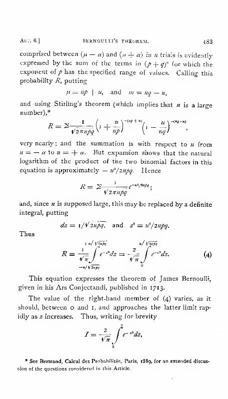
The value of the right-hand member of (4) varies, as it
should, between o and 1, and approaches the latter limit rap-
idly as z increases. Thus, writing for brevity
z
* See Bertrand, Calcul des Probabilities, Paris, 1889, for an extended discus-
sion of the questions considered in this Article.
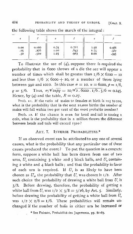
484 PROBABILITY AND THEORY OF ERRORS. [Chap. X.
the following table shows the march of the integral
:
s
Art. 7.] inverse probabilities. • 485
•diminished so long as the ratio of white to black balls is kept
constant. Make these numbers the same for the two urns.
Thus let the first contain 9 white and 15 black, and the second
8 white and 16 black; whence the above probabilities may be
written 1/2 x 9/24 and 1/2 X 8/24. It is now seen that there
are (9 -f- 8) cases favorable to the production of a white ball,
each of which has the same antecedent probability, namely, 1/2.
Since the fact that a white ball was drawn excludes considera-
tion of the black balls, the probability that the white ball came
from Uxis 9/17 and that it came from cT, is 8/17 ; and the sum
of these is unity, as it should be.
To generalize this result, let there be m causes, C,, C„ . . . Cm .
Denote their direct probabilities by qv q„ . .qm \their antecedent
probabilities by rlf ra , . . . rm \ and their resultant probabilities
on the supposition of separate existence by A>A> • • pm .
That is,
Pi = ?ir» A = 9S*> • • • A» = ?«*»• (0
Let D be the common denominator of the right-hand mem-
bers in (1), and denote the corresponding numerators of the
several fractions by s,, s„ . . . sm . Then
p, = sJD, p, = sJD, . . .pm = sm/D ;
and it is seen that there are in all (st -f- j
a-\- . . . sm ) equally
possible cases, and that of these sxare favorable to Clt s, to
C„ . . . Hence, if P„ P„ . . . Pm denote the probabilities of
the several causes on the supposition of their coexistence,
Pi = sj& + *.+ • • • J™) =A/(A +A + • • A,)-
Thus in general
P1= pj2p, P, = pJ?.p,...Pm =pm/2p. (2)
To illustrate the meaning of these formulas by the above
concrete case of the urns it suffices to observe that
for Ult q, = 3/8 and r, = 1/2,
for U„ q, = 1/3 and r, = 1/2 ;
whence p i= 3/16, /, = 1/6, /,+/,= 17/48 ;
and P,=9/i7, /", = 8/17.
As a second illustration, suppose it is known that a white
486 • PROBABILITY AND THEORY OF ERRORS. [CHAP. X.
ball has been drawn from an urn which originally contained mballs, some of them being black, if all are not white. What is
the probability that the urn contained exactly n white balls?
The facts are consistent with m different and equally probable
hypotheses (or causes), namely, that there were i white and
(m — i) black balls, 2 white and (m — 2) black balls, etc.
Hence in (1), ql= qt
= . . . = I, and
pl— i/m, p, = 2/m, . . . p„ — n/m, . . . pm = m/m.
Thus 2p = (i/2)(m+ 1),
2nand P„ = p„/2p = —
~, ,—\.
This shows, as it evidently should, that n = m is the most
probable number of white balls in the urn. The probability
for this number is Pm = 2/{m -\- 1), which reduces, as it ought,
to I for m=\.Formulas (1) and (2) may also be applied to the problem of
estimating the probability of the occurrence of an event from
the concurrent testimony of several witnesses, Xn X„ . . .
Denote the probabilities that the witnesses tell the truth by
xtx„ . . . Then, supposing them to testify independently,
the probability that they will concur in the truth concerning
the event is x^x, . . . ; while the probability that they will con-
cur in the only other alternative, falsehood, is (1 —x^i —xt) .
.
.
The two alternatives are equally possible. Hence by equations
(1) and (2)
p, = x,x, ..., p t— {l - 0(1 — *,) . . .,
X\X'„. . .
p.=
x,x, . . . + (I — *,)(i - xt) . . .'
XtX^ . . .+(1 - JT,)(l - X,) . .
.'
Pj being the probability for and P^ that against the event.
To illustrate (3), if the chances are 3 to 1 that X, tells the
truth and 5 to 1 that X, tells the truth, jtr, = 3/4, x, — 5/6, and
Pl= 15/16; or, the chances are 15 to 1 that an event occurred
if they agree in asserting that it did.*
* For some interesting applications of equations (3) see note E of Appendix
to the Ninth Bridgewater Treatise by Charles Babbage (London, 1838).
Art. 8.] probabilities of future events. 487
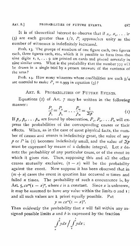
It is of theoretical interest to observe that if Xl , x , . . . ir
(3) are each greater than 1/2, Plapproaches unity as the
number of witnesses is indefinitely increased.
Prob. 13. The groups of numbers of one figure each, two figureseach, three figures each, etc., which it is possible to form from thenine digits 1, 2, ... 9 are printed on cards and placed severally innine similar urns. What is the probability that the number 777 will
be drawn in a single trial by a person unaware of the contents ofthe urns ?
Prob. 14. How many witnesses whose credibilities are each 3/4are essential to make P
t= 0.999 m equation (3) ?
Art. 8. Probabilities of Future Events.
Equations (2) of Art. 7 may be written in the following
manner:
5 = 5- 3l = _LA A Pm~W (I)
If A> A. • • • Pm are found by observation, P„ Pt , . . . Pm will ex-
press the probabilities of the corresponding causes or their
effects. When, as in the case of most physical facts, the num-ber of causes and events is indefinitely great, the value of any
p or P in (1) becomes indefinitely small, and the value of 2pmust be expressed by means of a definite integral. Let x de-
note the probability of any particular cause, or of the event to
which it gives rise. Then, supposing this and all the other
causes mutually exclusive, (1 — x) will be the probability
against the event. Now suppose it has been observed that in
(m -\- n) cases the event in question has occurred m times and
failed n times. The probability of such a concurrence is, by
Art. $,cxm(i — x)n, where c is a constant. Since x is unknown,
it may be assumed to have any value within the limits o and 1
;
and all such values are a priori equally possible. Put
y = cx'"(i — x) n.
Then evidently the probability that x will fall within any as-
signed possible limits a and b is expressed by the fraction
o 1
I ydx I I ydx;
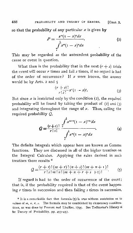
488 PROBABILITY AND THEORY OF ERRORS. [CHAP. X.
so that the probability of any particular x is given by
xm(l — xfdxP = ~7S "
•(2
)
/V"(i — xfdx
This may be regarded as the antecedent probability of the
cause or event in question.
What then is the probability that in the next (r -f- s) trials
the event will occur r times and fail s times, if no regard is had
of the order of occurrence ? If x were known, the answer.
would be by Arts. 2 and 5
(r-\-s)\ ,
But since x is restricted only by the condition (2), the required
probability will be found by taking the product of (2) and (3)
and integrating throughout the range of x. Thus, calling the
required probability Q,
fxm+r(i — x)n+sdx
6=^^; . (4)r\s\
fxm{\ — x)ndx
The definite integrals which appear here are known as Gammafunctions. They are discussed in all of the higher treatises on
the Integral Calculus. Applying the rules derived in such
treatises there results *
(r -\- s) ! (m -\- r) ! {n -\- s) ! (m -\- n -\- 1 )
!
^ ~ r\s\m\n\(m -{ n -\- r -\- s +1)! '
^'
If regard is had to the order of occurrence of the event
;
that is, if the probability required is that of the event happen-
ing r times in succession and then failing s times in succession,
* It is a remarkable fact that formula (5) is true without restriction as to
values of m, n, r, s. The formula may be established by elementary considera-
tions, as was done by Prevost and Lhuilier, 1795. See Todhunter's History of
he Theory of Probability, pp. 453-457.
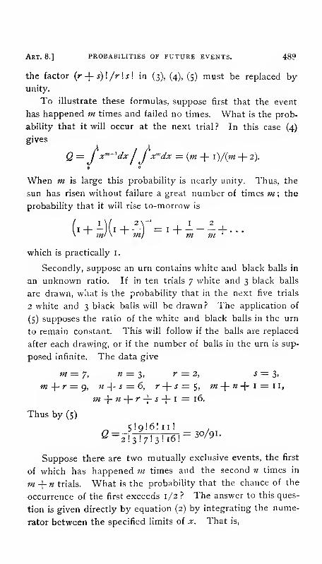
Art. 8.] probabilities of future events. 489
the factor (r -+- s)\/r\s\ in (3), (4), (5) must be replaced by
unity.
To illustrate these formulas, suppose first that the event
has happened m times and failed no times. What is the prob-
ability that it will occur at the next trial ? In this case (4)
gives
Q = fxm+1dxJJxmdx = (m+ i)/{m + 2).
When m is large this probability is nearly unity. Thus, the
sun has risen without failure a great number of times m ; the
probability that it will rise to-morrow is
(I+ i)(I+ i.r=I+ i_i+...
which is practically 1.
Secondly, suppose an urn contains white and black balls in
an unknown ratio. If in ten trials 7 white and 3 black balls
are drawn, what is the probability that in the next five trials
2 white and 3 black balls will be drawn? The application of
{5) supposes the ratio of the white and black balls in the urn
to remain constant. This will follow if the balls are replaced
after each drawing, or if the number of balls in the urn is sup-
posed infinite. The data give
m = j, n = 3, r = 2, s = 3,
m-{-r = g, n -\- s = 6, r -j- s = $, m-\- n-\- 1 = 11,
m-\-n-\-r-\-s-\-i = 16.
Thus by (5)
S!c.!6!n!Q =
2 ! 3 ! 7 ! 3 !i6! = 3o/9i.
Suppose there are two mutually exclusive events, the first
of which has happened m times and the second n times in
m-\-n trials. What is the probability that the chance of the
occurrence of the first exceeds 1/2 ? The answer to this ques-
tion is given directly by equation (2) by integrating the nume-
rator between the specified limits of x. That is,
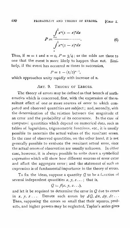
490 PROBABILITY AND THEORY OF ERRORS. [CHAP X.
i
/V*(i — xfdx_ 0.5
P=— •
(6)
fxm{\ —xfdx
Thus, if tn = i and n = o, P = 3/4 ; or the odds are three to
one that the event is more likely to happen than not. Simi-
larly, if the event has occurred m times in succession,
P= 1 -(1/2)™+',
which approaches unity rapidly with increase of n.
Art. 9. Theory of Errors.
The theory of errors may be defined as that branch of math-
ematics which is concerned, first, with the expression of the re-
sultant effect of one or more sources of error to which com-
puted and observed quantities are subject ; and, secondly, with
the determination of the relation between the magnitude of
an error and the probability of its occurrence. In the case of
computed quantities which depend on numerical data, such as
tables of logarithms, trigonometric functions, etc., it is usually
possible to ascertain the actual values of the resultant errors.
In the case of observed quantities, on the other hand, it is not
generally possible to evaluate the resultant actual error, since
the actual errors of observation are usually unknown. In either
case, however, it is always possible to write down a symbolical
expression which will show how different sources of error enter
and affect the aggregate error ; and the statement of such an
expression is of fundamental importance in the theory of errors.
To fix the ideas, suppose a quantity Q to be a function of
several independent quantities x, y, z . . .; that is,
Q=/(x,y, z...),
and let it be required to determine the error in Q due to errors
in x, y , z . . . Denote such errors by AQ, Ax, Ay, As .
Then, supposing the errors so small that their squares, prod-
ucts, and higher powers may be neglected, Taylor's series gives
Art. 10.] laws of error. 491
^ = t**+f/>+f^+-- <>
This equation may be said to express the resultant actual error
of the function in terms of the component actual errors, since
the actual value of AQ is known when the actual errors of
x, y, z . . . are known. It should be carefully noted that the
quantities x, y, z . . . are supposed subject to errors which are
independent of one another. The discovery of the independent
sources of error is sometimes a matter of difficulty, and in general
requires close attention on the part of the student if he would
avoid blunders and misconceptions. Every investigator in work
of precision should have a clear notion of the error-equation of
the type (i) appertaining to his work; for it is thus only that
he can distinguish between the important and unimportant
sources of error.
Prob. 15. Write out the error-equation in accordance with (1)
for the function Q — xyz -+- x3
log (y/z).
Prob. 16. In a plane triangle a/b = sin^/sin B. Find the error
in a due to errors in b, A, and B.
Prob. 17. Suppose in place of the data of problem 16 that the
angles used in computation are given by the following equations :
^=^+$(180°-^- B- Q, B = B, + |(i8o° - A-Bt
- C,),
where A u B l, C, are observed values. What then is Aa ?
Prob. 18. If w denote the weight of a body and r the radius of
the earth, show that for small changes in altitude, Aw/w = — Ar/r\
whence, if a precision of one part in 500000000 is attainable in com-
paring two nearly equal masses, the effect of a difference in altitude
of one centimeter in the scale-pans of a balance will be noticeable.*
Art. 10. Laws of Error.
A law of error is a function which expresses the relative
frequency of occurrence of errors in terms of their magnitudes.
Thus, using the customary notation, let e denote the magni-
* This problem arose with the International Bureau of Weights and Measures,
Whose work of intercomparison of the Prototype Kilogrammes attained a pre-
cision indicated by a probable error of 1/500 000 oooth part of a kilogramme.
492 PROBABILITY AND THEORY OF ERRORS. [Chap. X.
tude o. any error in a system of possible errors. Then the law
of such system may be expressed by an equation of the form
y = 0(e)- (i)
Representing e as abscissa and y as ordinate, this equation
gives a curve called the curve of frequency, the nature of which,
as is evident, depends on the form of the function 0. This
equation gives the relative frequency of occurrence of errors in
the system ; so that if e is continuous the probability of the
occurrence of any particular error is expressed by yde = cp(e)de;
which is infinitesimal, as it plainly should be, since in any con-
tinuous system the number of different values of e is infinite.
Consider the simplest form of 0(e), namely, that in which
0(e) = c, a constant. This form of 0(e) obtains in the case of
the errors of tabular logarithms, natural trigonometric func-
tions, etc. In this case all errors between minus a half-unit
and plus a half-unit of the last tabular place are equally likely
to occur. Suppose, to cover the class of cases to which that
just cited belongs, all errors between the limits — and -fa
are equally likely to occur. The probability of any individual
error will then be <p(e)de = cde, and the sum of all such prob-
abilities, by equation (2), Art. 4, must be unity. That is,
I cp(e)de = c I de — I.
-a _a
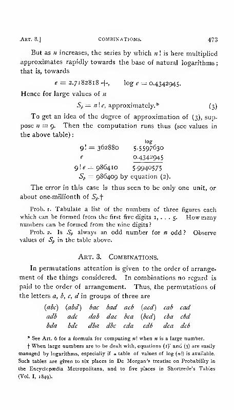
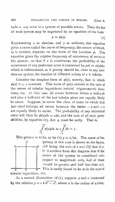
This gives c = \/2a, or by (1) y = \/2a. The curve of fre-
quency in this case is shown in the figure,
AB being the axis of e and OQ that of y.
It is evident from this diagram that if the
errors of the system be considered with
respect to magnitude only, half of them
should be greater and half less than a/2.
This is easily found to be so in the case of
tabular logarithms, etc.
As a second illustration of (1), suppose y and e connected
by the relation^ = c Vd2 — e"-, where a is the radius of a circle,
ART. 11.] TYPICAL ERRORS OF A SYSTEM. 493
c a constant, and e may have any value between — a and -f- a.
Then the condition
c J de Vd' — e" = i
gives c = 2/(a27t). In this, as in the preceding case, <p{-\- e) =
<p{— e), the meaning of which is that positive and negative
errors of the same magnitude are equally likely to occur. It
will be noticed, however, that in the latter case small errors
have a much higher probability than those near the limit a,
while in the former case all errors have the same probability.
In general, when e is continuous (p(e) must satisfy the condi-
tion / <p(e)de = I, the limits being such as to cover the entire
range of values of e. The cases most commonly met with are
those in which 0(e) is an even function, or those in which
0(+ e) = <P{— e)- I n sucn cases, if ± a denote the limiting
value of e,+ a a
C<p(e)de = 2f(j>(e)de = I. (3)
-a •
Art. 11. Typical Errors of a System.
Certain typical errors of a system have received special
designations and are of constant use in the literature of the
theory of errors. These special errors are the probable error,
the mean error, and the average error. The first is that error
of the system of errors which is as likely to be exceeded as
not ; the second is the square root of the mean of the squares
of all the errors ; and the third is the mean of all the errors
regardless of their signs. Confining attention to systems in
which positive and negative errors of the same magnitude
are equally probable, these typical errors are defined mathe-
matically as follows. Let
ep = the probable error,
em= the mean error,
ea = the average error.
494 PROBABILITY AND THEORY OF ERRORS. [CHAP. X.
Then, observing (2), of Art. 10,
f(p(e)de =J'(p(e)de = fcp(e)de =J<p(e)de = \.
+H
-_f(p{eyde, ea - 2Jt
<p(e)ede.
(0
The student should seek to avoid the very common misap-
prehension of the meaning of the probable error. It is not
" the most probable error," nor " the most probable value of
the actual error" ; but it is that error which, disregarding signs,
would occupy the middle place if all the errors of the system
were arranged in order of magnitude. A few illustrations will
suffice to fix the ideas as to the typical errors. Thus, take the
simple case wherein <p(e) = c= i/2a, which applies to tabular
logarithms, etc. Equations (1) give at once
et = ± -a, em = ± - Y 3 , ea = ± -a.p2 3 2
For the case of tabular values, a = 0.5 in units of the last
tabular place. Hence for such values
ep= ± 0.25, em —± 0.29, ea — ± 0.25.
Prob. 19. Find the typical errors for the cases in which the law
-of error is 0(e) = cVc? — e\ <f>(e) = c(±a^e), 4>(e)=c cos'(7te/2a);
c being a constant to be determined in each case and e having any
value between — a and + a.
Art. 12. Laws of Resultant Error.
When several independent sources of error conspire to pro-
duce a resultant error, as specified by equation (1) of Art. 9,
there is presented the problem of determining the law of the
resultant error by means of the laws of the component errors.
The algebraic statement of this problem is obtained as follows
for the case of continuous errors :
In the equation (1), Art. 9, write for brevity
e=AQ, e,=^z/*, e^-^Ay,.' . . ;
dx dy
Art. 12.] laws of resultant error. 495
and let the laws of error of e, et , <=„ . . . be denoted by 0(e),
0,(e,), 0,(ea) . . . Then the value of e is given by
«=*, + *,+•.. (i)
The probabilities of the occurrence of any particular values
of e„ e„,. . . are given by 0,(e.Ke .. 0,O»Kea> • • • ; and the
probability of their concurrence is the probability of the cor-
responding value of e. But since this value may arise in an
infinite number of ways through the variations of e,, e2 , . . .
over their ranges, the probability of e, or <p(e)de, will be
expressed by the integral of<f> 1
(el)de
l<j>i(e^de
l. . . subject to
the restriction (i). This latter gives e, = e— e2— e
3. . ., and
de1= de for the multiple integration with respect to e
3 , e„ . . .
Hence there results
(P(e)de = rfey0,(6 - e, - es- . . .)(f>t
(e,)de, ...,
or
0(0 = yW* -e, - e, - . . .)<j>t{et)de,f<j>t(e,)de
t... (2)
It is readily seen that this formula will increase rapidly in
complexity \vrith the number of independent sources of error.*
For some of the most important practical applications, how-
ever, it suffices to limit equation (2) to the case of two inde-
pendent sources of error, each of constant probability within
assigned limits. Thus, to consider this case, let e, vary over
the range — a to -\- a, and e2vary over the range — b to -\- b.
Then by equation (2), Art. 10,
0,(6.) = i/(2«),2(e
3)= \/{2b).
Hence equation (2) becomes
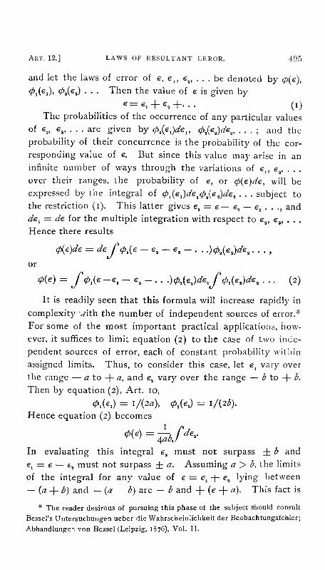
^= ibfde>-
In evaluating this integral e, must not surpass ± b and
e, = e — e, must not surpass ± a. Assuming ay b, the limits
of the integral for any value of e = e, -f- e, lying between
— (a-\- b) and — (a — b) are — b and -(- (e + «)• This fact is
* The reader desirous of pursuing this phase of the subject should consult
Bessel's Untersuchungen ueber die Wahrscheinlichkeit der Beobachtungsfehler;
Abhandlungen von Bessel (Leipzig, 1876), Vol. II.
496 PROBABILITY AND THEORY OF ERRORS. [CHAP. X.
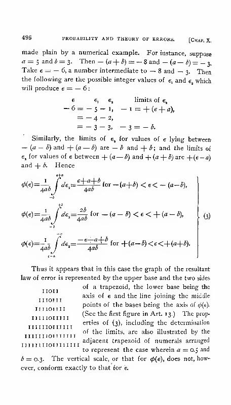
made plain by a numerical example. For instance, suppose
a = 5 and b = 3. Then — (a+ b) — — 8 and — (« — b) = -3.
Take e = — 6, a number intermediate to — 8 and — 3. Thenthe following are the possible integer values of e, and e which
will produce e = — 6
:
e e, e, limits of ea-6= -5 -1, -1 =+(e + «),
= - 4 - 2,
= -3-3. - 3 = - b.
Similarly, the limits of e, for values of e lying between
— (a — b) and + (a— b) are — b and + b ; and the limits of
e, for values of e between -f- (a— b) and + {a -f- b) are + (e — a)
and + b. Hence
0(e)=i/^=f=S? f°r -<«+*> < 6< ~ ('"'J'
-b
hfde<=3> i0r - {a -*)<6<+(a - d)'
-b
^bf^^r1 for +<«-*><«<+<«+*>•
*«>-£*
0(e)
I (3)
Thus it appears that in this case the graph of the resultant
law of error is represented by the upper base and the two sides-
of a trapezoid, the lower base being thenoil
, ,
axis of e and the line joining the middlemom.
points of the bases being' the axis of d>(e).iiiioiiii f
& w(See the first figure in Art. 13. ) The prop-iimoimi v &
,
J'
r r
erties of u), including the determinationimiioimii &
of the limits, are also illustrated by theiimiiomim J
adjacent trapezoid of numerals arrangedimiiiioniiim J
, .
b
to represent the case wherein a = 0.5 and
b = 0.3. The vertical scale, or that for 0(e), does not, how-
ever, conform exactly to that for e.
Art. 13.] errors of interpolated values. 497
Prob. 20. Prove that the values of 0(e) as given by equation (3)satisfy the condition specified in equation (3), Art. 10.
Prob. 21. Examine equations (3) for the case wherein a — b andb = o; and interpret for the latter case the first and last of (3).
Prob. 22. Find from (3), and (1) of Art. 11, the probable error of
the sum of two tabular logarithms.
Art. 13. Errors of Interpolated Values.
Case I.—One of the most instructive cases to which formulas
(3) of Art. 12 are applicable is that of interpolated logarithms,
trigonometric functions, etc., dependent on first differences.
Thus, suppose that vxand w
2are two tabular logarithms, and
that it is required to get a value v lying t tenths of the interval
from vxtowards vv Evidently
v =. vx + (y, — v
x) t = (1 - f)vx + tv
t ;
and hence if e, elf
e^ denote the actual errors of v, vlt z>2 , re-
spectively,
e={i-t)el + te
t. (1)
It is to be carefully noted here that e as given by (1) re-
quires the retention in v of at least one decimal place be-
yond the last tabular place. For example, let v = log (24373)
from a 5-place table. Then ^=4.38686, z', = 4.38703,
vt— v
t— -j-0.00017, t = 0.3, and v =4.38691.1. Likewise, as
found from a 7-place table, ex= — 0.45, e^ = -f- 0.37 in units of
the fifth place; and hence by (1) *= —0.20. That is, the
actual error of v = 4.38691. 1 is = 0.20, and this is verified by
reference to a 7-place table.
The reader is also cautioned against mistaking the species
of interpolated values here considered for the species common-
ly used by computers, namely, that in which the interpolated
value is rounded to the nearest unit of the last tabular place.
The latter species is discussed under Case II below.
Confining attention now to the class of errors specified by
equation (1), there result in the notation of the preceding
article
.
e, = (1 — t)ex , e
2= tev and e = e = e
x + e2 ;
and since e and e^ each vary continuously between the limits
498 PROBABILITY AND THEORY OF ERRORS. [CHAP. X.
± 0.5 of a unit of the last tabular place, a and b in equations
(3) of that article have the values
a = 0.5(1 — t), b =0.5/.
Hence the law of error of the interpolated values is ex-
pressed as follows
:
cp(e) = — for values of e betw. —0.5 and —(0.5—/),
for values of ebetw. — (0.5—^) and +(0.5—/),1 - t
— for values of e betw. +(0.5— () and +0.;.(1 - t)t
r\ a; t 3
(2)
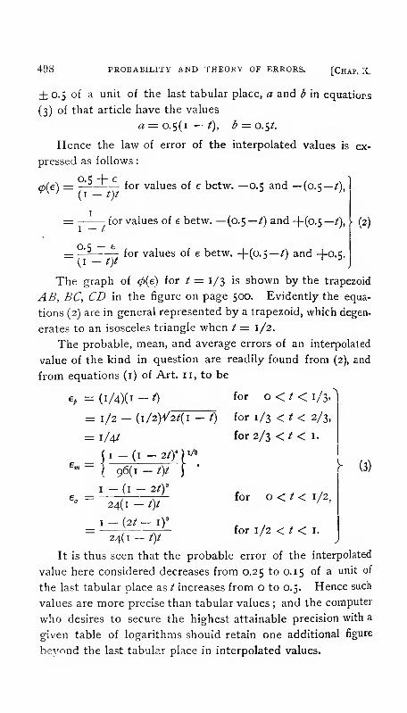
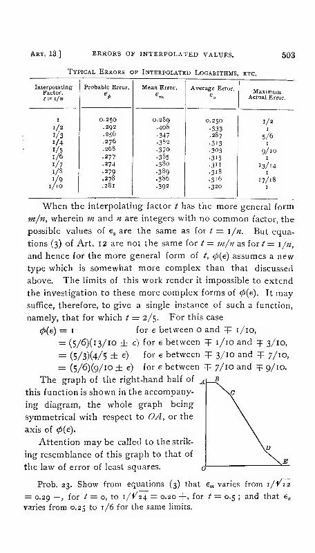
The graph of 0(e) for t = 1/3 is shown by the trapezoid
AB, BC, CD in the figure on page 500. Evidently the equa-
tions (2) are in general represented by a trapezoid, which degen-
erates to an isosceles triangle when t = 1/2.
The probable, mean, and average errors of an interpolated
value of the kind in question are readily found from (2), and
from equations (1) of Art. 11, to be
et = (l/4)(i ~t) for o < /? < 1/3/
= 1/2 - (i/2)V2*(i — t) for 1/3 < t < 2/3,
= i/4t for 2/3 < t < 1.
e-=i 96(1-/)/ \
- y (3)
1 - (1 - 2ty*a 7 a7~ for o < t < 1/2,
24(1 — t)t
I - (2t - I)3
for 1/2 < t < 1.
24(1 — f)t
It is thus seen that the probable error of the interpolated
value here considered decreases from 0.25 to 0.15 of a unit of
the last tabular place as t increases from o to 0.5. Hence such
values are more precise than tabular values ; and the computer
who desires to secure the highest attainable precision with a
given table of logarithms should retain one additional figure
beyond the last tabular place in interpolated values.
Art. 13.] errors of interpolated values. 499
Case II.—Recurring to the equation v = vt + t(v
t— v,) for an
interpolated value v in terms of two consecutive tabular values
vtand v„ it will be observed that if the quantity t(v, — v
t) is
rounded to the nearest unit of the last tabular place, a new error
is introduced. For example, if vx— log 1633 = 3.21299, and
vt= log 1634= 3.21325 from a 5-place table, z>, — », = + 26
units of the last tabular place ; and if t = 1/3, t(v1— v
t)= 8f ;
so that by the method of interpolation in question there results
v = 3.21299 -f 9 = 3.21308. Now the actual errors of z\ andv, are, as found from a 7-place table, — 0.38 and +0.21 in units
of the fifth place. Hence the actual error of v is by equation
0)» I X — 0.38 + \ X + 0.21 — \ = — 0.52, as is shown di-
rectly by a 7-place table.
It appears, then, that in this case the error-equation cor-
responding to (1) is
e=(i-t)el + te
t+e
t , (4)
wherein exand e^ are the same as in (1) and e,'\s the actual error
that comes from rounding t(vt— &,) to the nearest unit of the
last tabular place.
The error et , however, differs radically in kind from e
xand
<?2
. The two latter are continuous, that is, they may each have
any value, between the limits — 0.5 and +0.5 ; while e^ is dis-
continuous, being limited to a finite number of values depend-
ent on the interpolating factor t. Thus, for t — 1/2 the only
possible values of esare o -+- 1/2, and — 1/2 ; likewise for t =
1/3, the only possible values of esare o, -j- 1/3, and — 1/3. It
is also clear that the maximum value of e, which is constant and
equal to 1/2 for (1), is variable for (4) in a manner dependent
on t. For example, in (4),
The maximum of e = 1/2 + 1/2 = 1, for t = 1/2,
e = 1/2 + 1/3 = 5/6, " t = 1/3,
" " " e — 1/2 + 1/2 = 1, " t = 1/4,
" " " e= 1/2 + 2/5 = 9/10 " t — 1/5.
The determination of the law of error for this case presents
some novelty, since it is essential to combine the continuous
errors (1 — t)e, and te^ with the discontinuous error e,. The
500 PROBABILITY AND THEORY OF ERRORS. [ChAI?. X,
simplest mode of attacking the problem seems to be the fol-
lowing quasi-geometrical one. In the notation of Arts. 12 and
13, put in (4) e = e, (1 — f)ex— e,, te
t= e„ and e, = e
3. Then
e = (e. + e.) + 6.. (5)
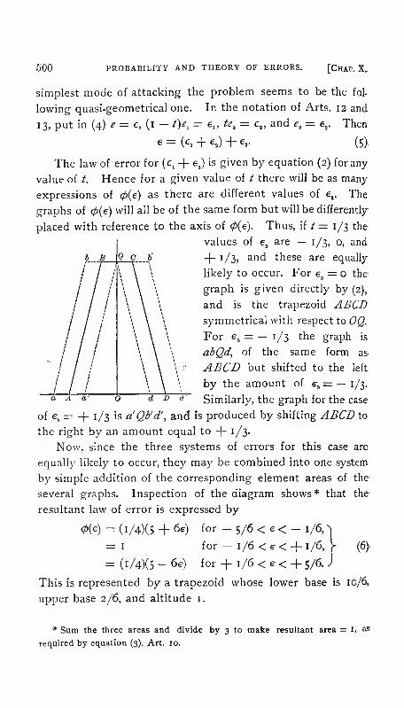
The law of error for (e, + es)
is given by equation (2) for any
value of t. Hence for a given value of t there will be as many
expressions of 0(e) as there are different values of e3
. The
graphs of 0(e) will all be of the same form but will be differently
placed with reference to the axis of 0(e). Thus, if t — 1/3 the
values of e3are — 1/3, o, and
-\- 1/3, and these are equally
likely to occur. For e3= the
graph is given directly by (2),
and is the trapezoid ABCDsymmetrical with respect to OQ.
For es= — 1/3 the graph is
abQd, of the same form as-
ABCD but shifted to the left
by the amount of e3= — 1/3.
Similarly, the graph for the case
of e3— -(- 1/3 is a'Qb'd', and is produced by shifting ABCD to
the right by an amount equal to -f- 1/3.
Now. since the three systems of errors for this case are
equally likely to occur, they may be combined into one system
by simple addition of the corresponding element areas of the
several graphs. Inspection of the diagram shows* that the-
resultant law of error is expressed by
0(e) = (1/4XS + 6e) for - 5/6 < e < - 1/6, >j
= 1 for - 1/6 < e < + 1/6, I (6)
= (1/4X5 -6e) for + i/6<e<+ S/6.J
This is represented by a trapezoid whose lower base is 10/6,
upper base 2/6, and altitude 1.
* Sum the three areas and divide by 3 to make resultant area = 1, as-
required by equation (3), Art. 10.
Art. 13.] ERRORS OF INTERPOLATED VALUES. 501
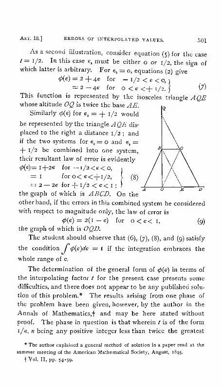
As a second illustration, consider equation (5) for the case
/ = 1/2. In this case es must be either o or 1/2, the sign of
which latter is arbitrary. For es= o, equations (2) give
0(e) = 2 + 4e for - 1/2 < e < o, \
= 2 — 4e for o < e <-f 1/2. \(7)
This function is represented by the isosceles triangle AQEwhose altitude OQ is twice the base AE.
Similarly 0(e) for ea= + 1/2 would
be represented by the triangle AQE dis-
placed to the right a distance 1/2 ; and
if the two systems for e3= o and e
3=
-|- 1/2 be combined into one system,
their resultant law of error is evidently
•0(e)= i-j-2e for — i/2<e< o, \
= 1 foro< e<-f-i/2, l (8)
= 2 — 2e for -j- 1/2 < e< 1 ; )
the graph of which is ABCD. On the
other hand, if the errors in this combined system be considered
with respect to magnitude only, the law of error is
0(e) = 2(1 - e) for o < e< 1, (9)
the graph of which is OQD.The student should observe that (6), (7), (8), and (9) satisfy
the condition / cp{e)de = 1 if the integration embraces the
whole range of e.
The determination of the general form of 0(e) in terms of
the interpolating factor t for the present case presents some
difficulties, and there does not appear to be any published solu-
tion of this problem.* The results arising from one phase of
the problem have been given, however, by the author in the
Annals of Mathematics,f and may be here stated without
proof. The phase in question is that wherein t is of the form
i/n, n being any positive integer less than twice the greatest
* The author explained a general method of solution in a paper read at the
summer meeting of the American Mathematical Society, August, 1895.
t "Vol. II, pp. 54-59.
502 PROBABILITY AND TH-EORY OF ERRORS. [Chap. X
tabular difference of the table to which the formulas are ap-
plied. For this restricted form of t the possible maximumvalue of e as given by equation (5) is, in units of the last
tabular place, (2« — \)Jn for n odd and 1 for n even.
The possible values of e3of equation (5) are
1 2 n — 1
O, ± -, ± -, . . . ± —
—
for n odd,I
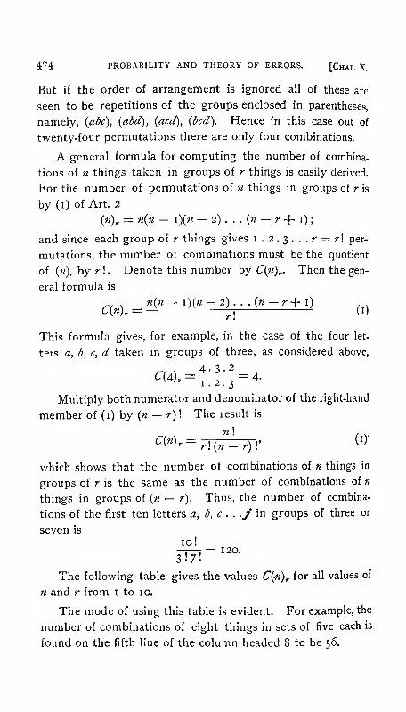
Art. 13.] errors of interpolated values. 503
Typical Errors of Interpolated Logarithms, etc.
InterpolatingFactor.
504 PROBABILITY AND THEORY OF ERRORS. [Chap. X.
Prob. 24. Show that the probable, mean, and average errors
for the case of t — 2/5 cited above (p. 503) are ± 0.261, ± 0.251,
and ± 0.290, respectively.
Art. 11. Statistical Test of Theory.
A statistical test of the theory developed in Art. 13 may
be readily drawn from any considerable number of actual er-
rors of interpolated values dependent on the same interpolating
factor. The application of such a test, if carried out fully by
the student, will go far also towards fixing clear notions as to
the meaning of the critical errors.
Consider first the case in which an interpolated value falls
midway between two consecutive values, and suppose this
interpolated value retains two additional figures beyond the
last tabular place. Then by equations (2), Art. 13, the law of
error of this interpolated value is
0(e) = 2 -|- 46 for e between — 0.5 and o
= 2 — 4e for e between o and -\- 0.5.
Hence by equation (1) of Art. 1 1, or equation (3) of Art. 12, the
probable error in this system of errors is \ — (£) 4/2 = 0.15.
It follows, therefore, that in any large number of actual errors
of this system, half should be less and half greater than 0.15.
Similarly, of the whole number of such errors the percentage
falling between the values 0.0 and 0.2 should beH-0-2 +0-2
J <p(e)de = 2J (2 — ^e)de = 0.64
;
_ 0.2
that is, sixty-four per cent of the errors in question should be
less numerically than 0.2.
To afford a more detailed comparison in this case, the act-
ual errors of five hundred interpolated values from a 5-place
table have been computed by means of a 7-place table. The
arguments used were the following numbers : 20005, 20035,
20065, 20105, 20135, etc., in the same order to 36635. The
actual and theoretical percentages of the whole number of
errors falling between the limits 0.0 and 0.1, 0.1 and 0.2, etc.,
are shown in the tabular form following
:
Art. 14.] statistical test of theory. 505
Limits of Errors. _ Act"al TheoreticalPercentage. Percentage.
o.oando.i 33.2 36
0.1 and 0.2 30.2 28
0.2 and 0.3 19.0 20
0.3 and 0.4 13.2 12
0.4 and 0.5 4.4 40.0 and 0.15 51.4 50
The agreement shown here between the actual and theoretical
percentages is quite close, the maximum discrepancy being 2.8
and the average 1.5 per cent.
Secondly, consider the case of interpolated mid-values of the
species treated under Case II of Art. 13. The law of error for
this case is given by the single equation (9) of Art. 13, namely,
<t>(e) — 2(1 — e), no regard being paid to the signs of the errors.
The probable error is then found from
2f(l ~ e)^e = h
whence eP = 1 — \ V2 = 0.29. Similarly, the percentage of
the whole number of errors which may be expected to lie, for
example, between 0.0 and 0.2 in this system is
0.2
2 / (1 — e)de = 0.36.
Using the same five hundred interpolated values cited
above, but rounding them to the nearest unit of the last tabu-
lar place and computing their actual errors by means of a 7-place
table, the following comparison is afforded :
T . . , _ Actual TheoreticalLimits of Errors. Percentage. Percentage.
0.0 and 0.2 35-8 36
0.2 and 0.4 27.8 28
0.4 and 0.6 18.6 20
0.6 and 0.8 12.2 12
0.8 and 1.0 5-6 4
O.o and 0.29 49-8 5°
506 PROBABILITY AND THEORY OF ERRORS. [Chap. X.
The agreement shown here between the actual and theoretical
percentages is somewhat closer than in the preceding case, the
maximum discrepancy being only 1.6 and the average only 0.6
per cent.
Finally, the following data derived from one thousand act-
ual errors may be cited. The errors of one hundred inter-
polated values rounded to the nearest unit of the last tabular
place were computed * for each of the interpolating factors
0.1, 0.2, . . . 0.9. The averages of these several groups of act-
ual errors are given along with the corresponding theoretical
errors in the parallel columns below
:
Interpolating Actual Theoretical
Factor. Average Error. Average Error.
O. I O.338 O.32O
0.2 O.288 O.303
O.3 O.32I O.304
O.4 O.268 O.29O
0.5 O.324 O.333
0.6 0.276 0.290
0.7 0.321 0.304
0.8 0.289 0.303
0.9 0.347 0.320
The average discrepancy between the actual and theoret-
ical values shown here is 0.017. It is, perhaps, somewhat
smaller than should be expected, since the computation of the
actual errors to three places of decimals is hardly warranted
by the assumption of dependence on first differences only.
The average of the whole number of actual errors in this
case is 0.308, which agrees to the same number of decimals
with the average of the theoretical errors, f
* By Prof. H. A. Howe. See Annals of Mathematics, Vol. Ill, p. 74-
The theoretical averages were furnished to Prof. Howe by the author,
\ The reader who is acquainted with the elements of the method of least
squares will find it instructive to apply that method to equation (1), Art. 13,
and derive the probable error of e. This is frequently done without reserve by
Art. 14.] statistical test of theory. 507
Prob. 25. Apply formulas (3) of Art. 12 to the case of the sumor difference of two tabular logarithms and derive the correspond-
ing values of the probable, mean, and average errors. The graph
of 0(e) is in this case an isosceles triangle whose base, or axis of e,
is 2, and whose altitude, or axis of 0(e), is 1.
those familiar with least squares. Thus, the probable error of et or ei being
0.25, tne probable error of e is found to be
0.25 Vl — 2/ -\- 21 1.
This varies between 0.25 for /= o and 0.1S for t = £ ; while the true value of
the probable error, as shown by equations (3), Art. 13, varies from 0.25 to 0.15
for the same values of t. It is, indeed, remarkable that the method of least
squares, which admits infinite values for the actual errors ei and e^, should give
so close an approximate formula as the above for the probable error of e.
Similarly, one accustomed to the method of least squares would be inclined
to apply it to equation (4), Art. 13, to determine the probable error of e. The
natural blunder in this case is to consider eu ei , and es independent, and e s like
ei and ei continuous betweer the limits 0.0 and 0.5 ;and to assign a probable
error of 0.25 to each. In t'..is manner the value
0.25^2(1 - t + t*)
is derived. But this is absurd, since it gives 0.25 V2 instead of 0.25 for t = o.
The formula fails then to give even approximate results except for values of t
near 0.5.