chapter03a - linear triangles.ppt - The University of Memphis · One of the most useful differential equations for engineers is Laplace’s equation. Pierre-Simon, marquis de Laplace

One of the most useful differential equations for engineers isLaplace’s equation.

Pierre-Simon, marquis de Laplace (March 23, 1749 – March 5, 1827) was a French mathematician and astronomer whose work was pivotal to the development of mathematical astronomy and statistics.

TWO-DIMENSIONAL BOUNDARY VALUE PROBLEMS

He formulated Laplace's equation, and pioneered the Laplace transform which appears in many branches of mathematical physics, a field that he took a leading role in forming.

The Laplacian differential operator, widely used in applied mathematics, is also named after him.

Laplace’s equation can describe torsion in solids, flow in porous media, steady state heat transfer, incompressible flow of inviscid fluids, electrostatic problems, and magneto-statics.

The general form of Laplace’s equation in Cartesian coordinates:


2 22

2 20

u uu

x y

The partial differential operator, 2, or ∆, (which may be defined in any number of dimensions) is called the Laplace operator, or just the Laplacian.


The nonhomogeneous form of Laplace’s equation is calledthe Poisson equation:

2 22

2 20

u uu f f

x y

Siméon-Denis Poisson (June 21, 1781 – April 25, 1840), was a French mathematician, geometer, and physicist.

Poisson's well-known correction of Laplace's second order partial differential equation for potential was first published in the Bulletin de la société philomatique (1813).

Each of the physical problems mentioned above involve either equilibrium or time independent states.

This type of problem is called an elliptic boundary value problem.

In general, a two-dimensional elliptic boundary value problem has the form:


2 , , 0 inu x y f x y

1onu g s

2onu

s u h sn

Where is the interior domain, and 1 and 2 form the boundary of the domain.


2 0u f

1

2

u g s

us u h s

n

s

A boundary condition that specifies the value of the function u on the surface 1 is called a Dirichlet (dee ree KLAY) boundary condition or type one condition.


us u h s

n

2 0u f

u g s

1

2

s

CIVL 8/7111 2-D Boundary Value Problems - Triangular Elements 1/14

us u h s

n

2 0u f

u g s

1

2

s

Johann Peter Gustav Lejeune Dirichlet (February 13, 1805 –May 5, 1859) was a German mathematician credited with the modern formal definition of a function


A boundary condition prescribed in the form of a derivative of the function u on the surface 2 is called a type two or a Neumann boundary condition.


us u h s

n

2 0u f

u g s

1

2

s

Carl Gottfried Neumann (May 7, 1832 - March 27, 1925) was a German mathematician. Neumann worked on the Dirichlet principle, and can be considered one of the initiators of the theory of integral equations.


us u h s

n

2 0u f

u g s

1

2

s

If the value of is not zero then the condition is called a Robins boundary condition.


us u h s

n

2 0u f

u g s

1

2

s

Victor Gustave Robin (1855-1897) was a French mathematical analyst and applied mathematician who lectured in mathematical physics at the Sorbonne in Paris and also worked in the area of thermodynamics.


us u h s

n

2 0u f

u g s

1

2

s

If the entire boundary is a type one boundary condition, then the boundary value problem is called a Dirichlet Problem.


us u h s

n

2 0u f

u g s

1

2

s


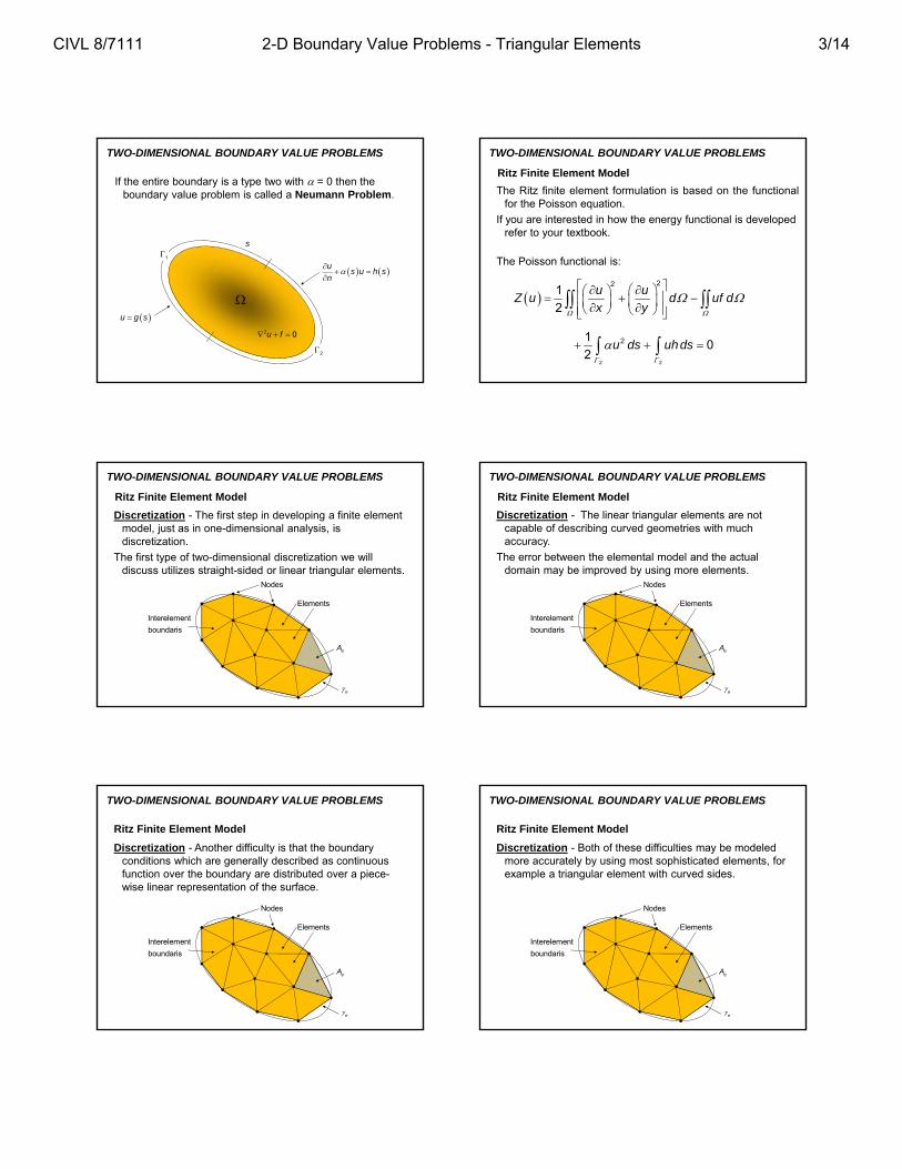
If the entire boundary is a type two with = 0 then the boundary value problem is called a Neumann Problem.


us u h s

n

2 0u f

u g s

1

2

s

Ritz Finite Element Model


The Ritz finite element formulation is based on the functionalfor the Poisson equation.

If you are interested in how the energy functional is developed refer to your textbook.

The Poisson functional is:

22

1

2

u uZ u d uf d

x y

2 2

210

2u ds uhds


Discretization - The first step in developing a finite element model, just as in one-dimensional analysis, is discretization.

The first type of two-dimensional discretization we will discuss utilizes straight-sided or linear triangular elements.

Interelement

boundaris

Nodes

Elements

e

eA



Discretization - The linear triangular elements are not capable of describing curved geometries with much accuracy.

The error between the elemental model and the actual domain may be improved by using more elements.

e

eA

Elements

Nodes

Interelement

boundaris




Discretization - Another difficulty is that the boundary conditions which are generally described as continuous function over the boundary are distributed over a piece-wise linear representation of the surface.

e

eA

Elements

Nodes

Interelement

boundaris



Discretization - Both of these difficulties may be modeled more accurately by using most sophisticated elements, for example a triangular element with curved sides.

e

eA

Elements

Nodes

Interelement

boundaris




Discretization - In terms of the discretization, the functional Z may be represented by a sum of the integrals over each element area Ae and each elemental surface e as:

22

1

2e e

e eA A

u uZ u dA uf dA

x y

2 2

21' ' 0

2e e

e e

u ds uhds

Where the sum is over all the elements, and ’ is over each elemental segment 2e of the 2 portion of the surface.

x

y

u



Interpolation - The simplest interpolation over a straight-sided three node triangular element is to assume the function u(x, y) is represented by a linear plane.

,k kx y

,i ix y

,j jx yeA

ku

iu

ju

Linear representation of

,eu x y



Interpolation - In a manner similar to that used to develop the linear, quadratic, and cubic shape functions for one-dimensional problems, we may describe the variation of uover the element as:

,eu x y x y

where , , and are constants determined by matching the function ue with the nodal values of the element:

,e i i i i iu x y x y u

,e j j j j ju x y x y u

,e k k k k ku x y x y u



Interpolation - Solving the three equations for , , and and substituting back into the expression representing the variation of u over the element results in:

where:

,e i i j j k ku x y N u N u N u

1, 2, 32

i i ii

e

a b x c yN i

A

with i j k k j i j k i k ja x y x y b y y c x x

where i, j, and k are permuted cyclically

i

j k



Interpolation - As before the functions N are called the shape functions. The determinant of the coefficients is:

where Ae is the area of the element.

Any numbering scheme that proceeds counterclockwise around the element is valid, for example (i, j, k), (j, k, i), or (k, i, j).

This numbering convention is important and necessary in order to compute a positive area for Ae.

1

2 1

1

i i

e j j

k k

x y

A x y

x y

i

j k



Interpolation - In matrix notation, the distribution of the function over the element is:

The linear triangular shape functions are illustrated below:

,eu x y T Te eu N N u

x y

iN

i

j

k

1

x y

jN

i

j

k

1x y

kN

i

j

k

1




Interpolation - The derivatives of u over the element with respect to both coordinates are:

Calculating the derivatives of the shape functions gives:

,eu x y

x x x

TT

e e

N Nu u

2 ex A

ebN

i j kb b bTeb

,eu x y

y y y

TT

e e

N Nu u

2 ey A

ecN

i j kc c cTec

i j kb y y i k jc x x



Interpolation - Observing the form of the derivative it is apparent that the partial derivatives of the function u will be constant over a linear triangular element.

There are many problems associated with accuracy and convergence for this type of element.

In elasticity analysis, stress and strain are related by a partial differential equation, using a linear triangular element to described stress will result in a constant approximation for strain over the element.

Therefore, elements of this type are called constant strain elements.



Elemental Formulation - The functional for the Poisson equation is:

We can write the functional in the following form:

2 2

21' ' 0

2e e e

e e eA

u ds uf dA uhds

22

1

2e

e A

u uZ u dA

x y

1 23 4' '

2 2e e

e ee e e e

Z ZZ u Z Z



Elemental Formulation – Where the components are defined as:

22

1

e

e

A

u uZ dA

x y

3

e

e

A

Z uf dA

2

22

e

eZ u ds

2

4

e

eZ uhds



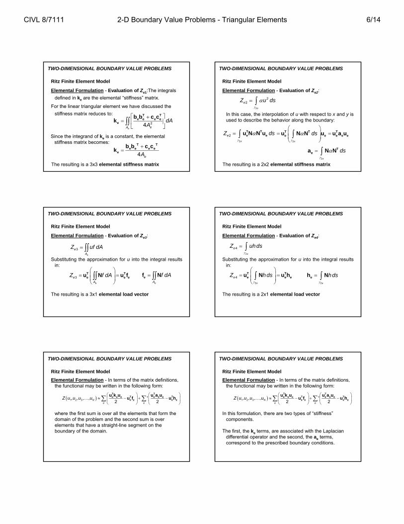
Elemental Formulation - Evaluation of Ze1:

Recall the first derivatives of u with respect to x and y are:

1eA

u u u uZ dA

x x y y

,eu x y

x

x

T

e

Nu

x

T

e

Nu

,eu x y

y

y

T

e

Nu

y

T

e

Nu



Elemental Formulation - Evaluation of Ze1: Replacing the

derivatives with the above approximations gives:

1eA

Z dAx x y y

T TT Te e e e

N N N Nu u u u

A

dAx x y y

T T

Te e

N N N Nu u

A

dAx x y y

T T

e

N N N Nk

Te e eu k u




Elemental Formulation - Evaluation of Ze1:The integrals

defined in ke are the elemental “stiffness” matrix.

For the linear triangular element we have discussed the

stiffness matrix reduces to:

Since the integrand of ke is a constant, the elemental stiffness matrix becomes:

24e eA

dAA

T Te e e e

e

b b c ck

4 eA

T Te e e e

e

b b c ck

The resulting is a 3x3 elemental stiffness matrix




In this case, the interpolation of u with respect to x and y isused to describe the behavior along the boundary:

2

22

e

eZ u ds

2

2

e

eZ ds

T Te eu N N u

2e

ds

T T T

e e e e eu N N u u a u

2e

ds

Tea N N

The resulting is a 2x2 elemental stiffness matrix




Substituting the approximation for u into the integral resultsin:

3

e

e

A

Z uf dA

3

e

eA

Z f dA

T T

e e eu N u feA

f dA ef N

The resulting is a 3x1 elemental load vector




Substituting the approximation for u into the integral resultsin:

The resulting is a 2x1 elemental load vector

2

4

e

eZ uhds

2

4

e

eZ hds

T T

e e eu N u h2e

hds

eh N



Elemental Formulation - In terms of the matrix definitions, the functional may be written in the following form:

where the first sum is over all the elements that form the domain of the problem and the second sum is over elements that have a straight-line segment on the boundary of the domain.

1 2 3, , , , '2 2N

e e

Z u u u u

T T

T Te e e e e ee e e e

u k u u a uu f u h




In this formulation, there are two types of “stiffness” components.

The first, the ke terms, are associated with the Laplacian differential operator and the second, the ae terms, correspond to the prescribed boundary conditions.

1 2 3, , , , '2 2N

e e

Z u u u u

T T


u k u u a uu f u h





The right-hand side of the system equations is also formed from two components.

The fe terms correspond to the Poisson term of the differential equation.

The he terms handle any nonhomogeneous boundary conditions.

1 2 3, , , , '2 2N

e e

Z u u u u

T T


u k u u a uu f u h



Assembly - The assembly is denoted by the summation in the matrix equation. The global matrix form of the formulation is:

2

Z Z T

TG G GG G G

u K uu F u

'e e

G G GK k a

0i

Z

u

2i

Z

u

TG G e

G

K K uF G G GK u F

'e e

G G GF f h



Constraints - The constraints on the system equations are the forced boundary conditions u = g(s) on the surface 1.

These conditions are applied to the system equations in a manner similar to that discussed for one-dimensional problems.



Solution - Since there are two types of boundary conditions, there are three possible situations to consider when determining a solution to the system equations.

One case is when the entire boundary consists of Dirichlet boundary conditions, u = g(s).

In this situation, a unique solution may be found.



A second case where a unique solution is possible is when the boundary is composed of both Dirichlet and Neumann boundary conditions.




The one situation where a singular solution is obtained is when Neumann-type conditions are prescribed along the entire boundary.

In this case, only a derivative-type condition exists.

There are infinite solutions in this type of problem.





Computation of Derived Variables - The solution for the nodal values of u are often called the primary variables, whereas the derivatives and any other values based on the primary variables are called secondary or derived variables.

In this case the values of the function u are the primary variables and u/n = nx u/x + ny u/y is consider a secondary variable.

,eu x y

x x x

TT

e e

N Nu u

,eu x y

y y y

TT

e e

N Nu u

2 eA

Te eb u

2 eA

Te ec u


Evaluation of Matrices - Linear Triangular Elements

Recall the elemental matrices have the following form:

A

dAx x y y

T T

e

N N N Nk

2e

ds

Tea N N

eA

f dA ef N

2e

hds

eh N

4 eA

T Te e e e

e

b b c ck

The evaluation of these integrals over a general element Aecan be very tedious. In order to simplify the computation we will discuss and introduce a local set of coordinates called area coordinates.

Consider a general linear triangular element:



1I J KL L L

I I J J K Kx x L x L x L

I I J J K Ky y L y L y L

1JI KI J K e

e e e

AA AA A A A

A A A

Where LI, LJ, and LK are the area coordinates.

x

y

IJ

K

P

KA

IAJA

As point P approaches any point on line IK, the area AJ 0and therefore, LJ 0

As point P approaches point K, then AK Ae and LK 1

Solving the three equations, LI, LJ, and LK we find these area coordinates are equal to the linear triangular shape functions Ni, Nj, and Nk.



1I J KL L L

I I J J K Kx x L x L x L

I I J J K Ky y L y L y L

x

y

IJ

K

P

KA

IAJA

Where LI, LJ, and LK are the area coordinates.

From the area coordinate relationship:



1I J KL L L

We observe that if LI and LJ are known then LK = 1 - LI - LJ

Therefore we can write the variation of x and y with the areacoordinates as:

,k i k I j k J I Jx x x x L x x L x L L

,k i k I j k J I Jy y y y L y y L y L L

Evaluation of ke - Using the local or area coordinates in the integrals transform the elemental matrices as follows:



The differential area dA is a vector with magnitude dA anddirection normal to the element area, which in this case isk.

,A

dA G x y dx dyx x y y

T T

e

N N N Nk


Evaluation of ke - The vector dA is given by the determinant rule:



where:

0

0

I J I JI I I J J I

J J

i j k

x y x y x ydL dL dL dL

L L L L L L

x y

L L

dA dx dy k

I JI J

x xdL dL

L L

dx

I JI J

y ydL dL

L L

dy

| | I JdA dL dL J

Evaluation of ke - where |J| is defined as the determinant of:



Therefore, ke transformed into area coordinates is:

| | 2i k i kI Ie

j k j k

J J

x yx x y yL L

Ax x y yx y

L L

J

, , | |I J I J I Jx L L y L L dL dL ek G J

Evaluation of ke - To transform the partial derivatives /x and /y to functions of LI and LJ:



where J, /L, and /x are:

I I I

x y

L x L y L

J J J

x y

L x L y L

J

L x

I I I

J J J

x y

L L L xx y

yL L L

JL x

Evaluation of ke - Where J is called the Jacobian matrix of the transformation. The matrix form of the transformation may be inverted.



The matrix may be partitioned as:

1J J

L x x L

x y

1 2J JL L

where J1 and J2 are the first and second rows of J-1.

Evaluation of ke - The partial derivatives /x and /y may now be written entirely in terms of L. Therefore, the partial derivatives of the shape functions may be written as:



T TT

1 1

N NJ J

x L

T

1

NJ

x

JI K

I I IT

JI K

J J J

LL L

L L L

LL L

L L L

TN

L

T TT

2 2

N NJ J

y L

T

2

NJ

y

1 0 1

0 1 1

Evaluation of ke - Substituting all the pieces of the transformation in the ke terms gives:



| | I JdL dL T T T T

e 1 1 2 2k J J J J J

| | I JdL dL T T T

1 1 2 2J J J J J

where JJ = (J1TJ1 + J2

TJ2)|J|.

The integrand of the above integral is a constant, therefore,ke reduces to:

4 eA

T Te e e e

e

b b c ck

I JdL dL TJJ

The resulting elemental stiffness matrix ke is a 3 x 3


Evaluation of fe - In general, the integral fe is:



For a general function f(x,y), the above integral may be quitetedious to evaluate, therefore we will assume that f varieslinearly over the element, f(x,y) = NTf, where the vector fcontains values of the function f at the node points.

With this assumption the integral becomes:

,eA

f x y dA ef N

eA

dA Tef NN f

eA

dA

TNN f

Evaluation of fe - The formula for integrations of the type is given without proof as:



Therefore:e

a b cI J K

A

N N N dA

2 1 1

1 2 112

1 1 2

i

ej

k

fA

f

f

ef

The resulting is a 3 x 1 elemental load vector

2

! ! !2 !

eAa b c

a b c

2

212

2

i j k

ei j k

i j k

f f fA

f f f

f f f

ef

Evaluation of he - Consider the integral:



where the integration is along a boundary segment of theelement.

Since, the integration is computed along a single side of the triangular element, the original shape functions reduce to:

2e

hds

eh N

0 1I J KN N N

2

1

e

eh l d

eh

kh

jh

0

1 el

i

j

k

Evaluation of he - For a general function h() the integral may be tedious to evaluate, therefore we will assume that h varies linearly over the boundary.

Consider h() = NTh, where the vector h contains the values of the function h at the boundary node points.



0 1I J KN N N

2

1

e

eh l d

eh

kh

jh

0

1 el

i

j

k

Evaluation of he - With this assumption the integral becomes:



2e

el d

Teh NN h

2 1

1 26el

eh h

The formula for integrations of the type is the same as forthe ke term:

The resulting is a 2 x 1 elemental load vector

2

26j ke

j k

h hlh h

eh

2e

el d

TNN h

2 1

1 26je

k

hl

h

Evaluation of ae - The evaluation of ae is very similar that of he except that there is an extra NT in the integrand.

The variation of the function (s) will be approximated as jNj + kNk. Consider the integral ae:



The resulting is a 2 x 2 elemental stiffness matrix

2e

ds

Tea N N

2e

j j j k k j j j j k k k

e

k j j k k j k j j k k k

N N N N N N N Nl d

N N N N N N N N


Evaluation of ae - The integration formula for the type of integrals is:



The resulting 2 x 2 stiffness matrix contributes to the global system equations when the element has a side as part of the boundary.

2e

a bI JN N ds

3

312j k j ke

j k j k

l

ea

! !

1 !ela b

a b

Recall, the global system equations are composed from the following summations:



The resulting system equations are, in matrix form, given as:

'e e

G G GK k a

G G GK u F

'e e

G G GF f h


PROBLEM #16 - For a linear interpolation, verify that the two expressions for the elemental stiffness ke, given as:

are exactly the same.

| | I JdL dL T T T T

e 1 1 2 2k J J J J J

and

4 eA

T Te e e e

e

b b c ck


Example - Consider the problem of torsion of a homogeneous isotropic prismatic bar.

The general two-dimensional boundary-value problem is:

where the dependent variable is the Prandlt stress function, G is the shear modulus, and is the constant rate of twist along the axis of the bar.

The stress components are given in terms of the derivatives of the Prandlt stress function.

2 , 2 0 in

0 on

x y G

xz yzy x


Example - Consider the problem of torsion of a homogeneous isotropic prismatic bar.

The general two-dimensional boundary-value problem is:

The total torque transmitted along the bar is determined from:

2 , 2 0 in

0 on

x y G

2T dA


Example - The simplest model for torsion of a square bar, utilizing symmetry is a single triangular element.

The general problem domain and the FEM mesh are shown below.

0n

0

x

y

0n

X

Y

1

(0,0)

2

(1,0)

3

(1,1)

Lines of Symmetry

cross-sectional area

T



Example - Before beginning the FEM model, it is desirable to non-dimensionalize the problem.

22

x yX Y

a a G a

Therefore, the governing differential equation becomes:

2 1 1, 1 0 in

1 10 on

XX Y

Y

The stresses and torque for the Prandlt stress function are:

2 2xz yzG a G aY X

44T G a dXdY


Example - Elemental Formulation - Using a linear triangular element the elemental stiffness matrix components are:

where

In this example, node 1 is located at (X, Y) = (0, 0), node 2 at (1, 0), and node 3 at (1, 1), therefore:

4 eA

T Te e e e

e

b b c ck

2 3

3 1

1 2

Y Y

Y Y

Y Y

eb

1

1

0

eb

1 1 01

1 2 12

0 1 1

ek

3 2

1 3

2 1

X X

X X

X X

ec

0

1

1

ec1

2eA

i j kb y y

i k jc x x

0n

0

0n

X

Y

1

(0,0)

2

(1,0)

3

(1,1)


Example - Elemental Formulation - A loading function of f = 1 gives a load vector of:

Assembly - Since there is only one element in the model the assembly is simple:

2

212

2

i j k

ei j k

i j k

f f fA

f f f

f f f

ef

1 1 01

1 2 12

0 1 1

GK

1

2

3

1 1 0 11 1

1 2 1 12 6

0 1 1 1

11

16

1

11

16

1

GF


Example - Constraints - For this model, = 0 on the boundary, therefore, 2 and 3 = 0.

Solution - In this case, the solution is quite simple:

1

2

3

1 0 0 11 1

0 1 0 02 6

0 0 1 0

1

1

3

2

1

2

3

G a


Example - Computation of Derived Variables - The partial derivatives with respect to x and y that define the stress components are:

2xz G aY

2yz G aX

44T G a dXdY

4416

1.77789

G aT G a

4

1 2 3

48

3eG a A

2 02 e

G aA

T

e ec

22

2 3e

G aG a

A

T

e eb

48 4e

Te

A

G a N dX dY

4416

2.66676exact

G aT G a


Example - Computation of Derived Variables - The partial derivatives with respect to x and y that define the stress components are:

4 44 416 16

1.7778 2.66679 6exact

G a G aT G a T G a

1

0n

0

0n

X

Y

2

3

(0,0) (1,0)

(1,1)

1

X

Y

1

1(0,0)

2

(1,0)

3

(1,1)

eA



Example - Consider the same problem of torsion of a homogeneous isotropic prismatic bar as above except using a more refined mesh.

1

X

Y

(0,0) (1,0)

(1,1)

1 2

3

4

1

2

4

5

6

3

Lines of Symmetry

x

y

cross-sectional area

T


Example - Recall, the non-dimensional Poisson equation governing this problem.

22

x yX Y

a a G a

with

2 1 1, 1 0 in

1 10 on

XX Y

Y

The stresses and torque for the Prandlt stress function are:

2 2xz yzG a G aY X

44T G a dXdY



For element 1: node 1 is located at (X, Y) = (0, 0); node 2 at (0.5, 0); and node 3 at (0.5, 0.5).

4 eA

T Te e e e

e

b b c ck

2 3

3 1

1 2

Y Y

Y Y

Y Y

eb

11

12

0

1b

3 2

1 3

2 1

X X

X X

X X

ec

01

12

1

1c

1

1

2

3

1 1 01

1 2 12

0 1 1

k1

1

8A

1

X

Y

(0,0) (1,0)

(1,1)

1 2

3

4

1

2

4

5

6

3



For element 2: node 2 is located at (X, Y) = (0.5, 0); node 4 at (1, 0); and node 3 at (0.5, 0.5).

4 eA

T Te e e e

e

b b c ck

2

11

12

0

b

2

11

02

1

c

2

1

8A 2

2

4

3

2 1 11

1 1 02

1 0 1

k

2 3

3 1

1 2

Y Y

Y Y

Y Y

eb3 2

1 3

2 1

X X

X X

X X

ec

1

X

Y

(0,0) (1,0)

(1,1)

1 2

3

4

1

2

4

5

6

3



For element 3: node 3 is located at (X, Y) = (0.5, 0.5); node 4 at (1, 0); and node 5 at (1, 0.5).

4 eA

T Te e e e

e

b b c ck

2 3

3 1

1 2

Y Y

Y Y

Y Y

eb3 2

1 3

2 1

X X

X X

X X

ec

3

11

02

1

b

3

01

12

1

c

3

1

8A 3

3

4

5

1 0 11

0 1 12

1 1 2

k

1

X

Y

(0,0) (1,0)

(1,1)

1 2

3

4

1

2

4

5

6

3



For element 4: node 3 is located at (X, Y) = (0.5, 0.5); node 5 at (1, 0.5); and node 6 at (1, 1).

4 eA

T Te e e e

e

b b c ck

2 3

3 1

1 2

Y Y

Y Y

Y Y

eb3 2

1 3

2 1

X X

X X

X X

ec

4

11

02

1

b

4

01

12

1

c

4

1

8A 4

3

5

6

1 1 01

1 2 12

0 1 1

k

1

X

Y

(0,0) (1,0)

(1,1)

1 2

3

4

1

2

4

5

6

3



Example - Elemental Formulation - The loading function of f = 1 gives a series of elemental load vectors of:

Assembly - Since there are four elements in the model the assembly is not difficult:

2

212

2

i j k

ei j k

i j k

f f fA

f f f

f f f

ef

1

2

3

4

5

6

1 1 0 0 0 0 1

1 4 2 1 0 0 2

0 2 4 0 2 0 41 1

0 1 0 2 1 0 22 24

0 0 2 1 4 1 2

0 0 0 0 1 1 1

11

124

1

1 2 3 4f f f f

Element 1

1

X

Y

(0,0) (1,0)

(1,1)

1 2

3

4

1

2

4

5

6

3

Element 2

Element 3 Element 4


Example - Constraints - For this model, = 0 on the boundary, therefore, 4, 5, and 6 = 0.

Solution - Solving the above equations gives:

1

2

3

4

5

6

1 1 0 0 0 0 1

1 4 2 0 0 0 2

0 2 4 0 0 0 41 1

0 0 0 1 0 0 02 24

0 0 0 0 1 0 0

0 0 0 0 0 1 0

1 2 3

14 10 9

48 48 48

2 2 2

1 2 3

28 20 18

48 48 48

G a G a G a

22G a


Example - Computation of Derived Variables - The total torque may be calculated as:

44T G a dXdY

44

1 2 31

48

3e

e e ee

G a AT

41.9444T G a

X

Y

1

1(0,0) 2 (1,0)

3(1,1)

4

5

6

1

X

Y

(0,0) (1,0)

(1,1)

1 2

3

4

1

2

4

5

6

3

48 4e

Te

A

G a N dX dY

42,240

1,152

G a

4416

2.66676exact

G aT G a


PROBLEMS #17 - For the mesh shown below set up and solve the torsion problem for the circle. Compare your results for the maximum shear stress and the total torque T with the exact solution.

Should the answers depend upon the angle ?

What boundary conditions should be used on the radial lines of the model?

Check to see how well these boundary conditions are satisfied.

0

1 2

3

4

cosr

Xa

sinr

Ya

1,0

2 2,

2 2

r a

X

Y

421

3

5


PROBLEM #18 - Repeat Problem #17 using 4, 8, and 16 triangular elements.

Utilize the program POIS36 given out in the class to perform your analysis.

Compare your results for the maximum shear stress and the total torque T with the exact solution.

End of

Chapter 3a


Documents

chapter03a - linear triangles.ppt - The University of Memphis · One of the most useful differential equations for engineers is Laplace’s equation. Pierre-Simon, marquis de Laplace