Embed Size (px)
Citation preview
Office of Graduate StudiesUniversity of South Florida
Tampa, Florida
CERTIFICATE OF APPROVAL__________________________
Master’s Thesis__________________________
This is to certify that the Master’s Thesis of
BADRI RATNAM
with a major in Mechanical Engineering has been approvedfor the thesis requirement on August 7, 2000
for the Master of Science in Mechanical Engineering degree.
Examining Committee:
_________________________________________________Co-Major Professor: Glen H. Besterfield, Ph.D.
_________________________________________________Co-Major Professor: Autar K. Kaw, Ph.D.
_________________________________________________Member: Roger A. Crane, Ph.D.
i

ii
PARAMETRIC FINITE ELEMENT MODELING OF TRUNNION HUB GIRDER
ASSEMBLIES FOR BASCULE BRIDGES
by
BADRI RATNAM
A thesis submitted in partial fulfillmentof the requirements for the degree of
Master of Science in Mechanical EngineeringDepartment of Mechanical Engineering
College of EngineeringUniversity of South Florida
December 2000
Co-Major Professor: Glen H. Besterfield, Ph.D.Co-Major Professor: Autar K. Kaw, Ph.D.
iii

DEDICATION
To my family, who have made countless sacrifices for me. Their love and
encouragement has helped me scale several heights and seek even more challenging ones
for the future.
iv
ACKNOWLEDGEMENTS
I wish to express my gratitude and thanks to Dr. Glen Besterfield whose guidance
and support served as catalyst for the successful completion of this work. His scholarly
advice, in particular in the field of finite element method proved invaluable. I am greatly
indebted to him for arranging the financial support, academic and computer resources
required for this work.
I also wish to thank Dr. Autar Kaw for his guidance and advice towards the
successful completion of this work. My discussions with him helped me see new
approaches to issues in this study and remove impediments as they came up.
I thank Dr. Roger Crane for serving on my committee.
I wish to thank Dr. Rajiv Dubey for his encouragement as the Chairman of the
Department of Mechanical Engineering. I owe a special thanks to Ms. Sue Britten,
Office Manager of the Department of Mechanical Engineering, for swiftly resolving
administrative issues. Thanks also to Becky Yettaw, Office Assistant for helping me in
times of need.
I also wish to thank my friends for all the help rendered during this project.
v
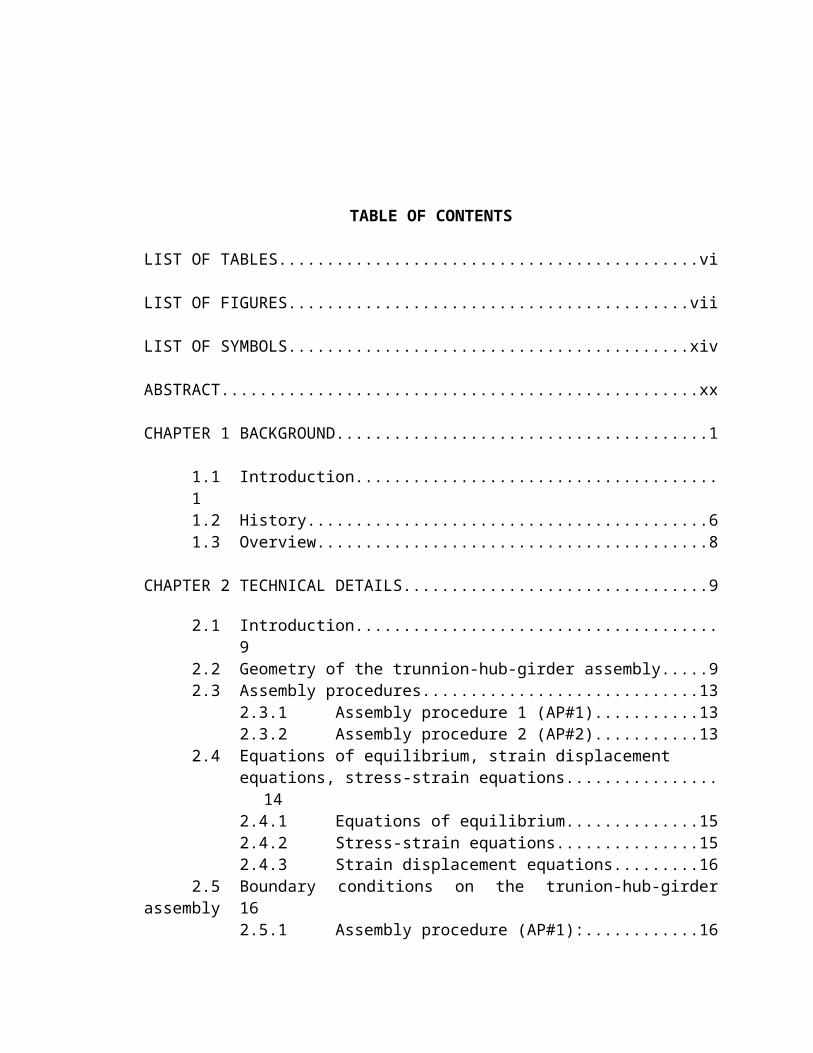
TABLE OF CONTENTS
LIST OF TABLES..............................................................................................................vi
LIST OF FIGURES...........................................................................................................vii
LIST OF SYMBOLS........................................................................................................xiv
ABSTRACT.......................................................................................................................xx
CHAPTER 1 BACKGROUND.........................................................................................1
1.1 Introduction..................................................................................................11.2 History..........................................................................................................61.3 Overview......................................................................................................8
CHAPTER 2 TECHNICAL DETAILS.............................................................................9
2.1 Introduction..................................................................................................92.2 Geometry of the trunnion-hub-girder assembly...........................................92.3 Assembly procedures.................................................................................13
2.3.1 Assembly procedure 1 (AP#1).......................................................132.3.2 Assembly procedure 2 (AP#2).......................................................13
2.4 Equations of equilibrium, strain displacement equations, stress-strain equations....................................................................................................142.4.1 Equations of equilibrium................................................................152.4.2 Stress-strain equations...................................................................152.4.3 Strain displacement equations........................................................16
2.5 Boundary conditions on the trunion-hub-girder assembly.........................162.5.1 Assembly procedure (AP#1):.........................................................16
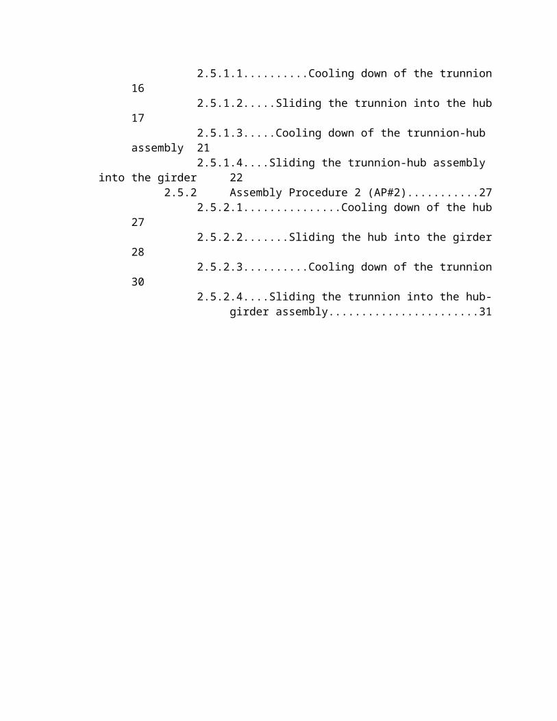
2.5.1.1 Cooling down of the trunnion............................................162.5.1.2 Sliding the trunnion into the hub.......................................172.5.1.3 Cooling down of the trunnion-hub assembly ....................212.5.1.4 Sliding the trunnion-hub assembly into the girder.............22
2.5.2 Assembly Procedure 2 (AP#2).......................................................272.5.2.1 Cooling down of the hub....................................................272.5.2.2 Sliding the hub into the girder...........................................282.5.2.3 Cooling down of the trunnion............................................302.5.2.4 Sliding the trunnion into the hub-girder assembly.............31

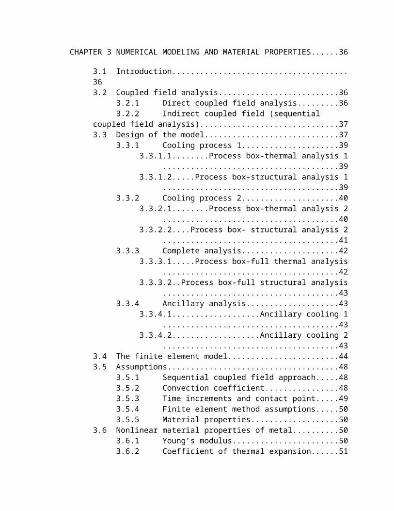
CHAPTER 3 NUMERICAL MODELING AND MATERIAL PROPERTIES.............36
3.1 Introduction................................................................................................363.2 Coupled field analysis................................................................................36
3.2.1 Direct coupled field analysis..........................................................363.2.2 Indirect coupled field (sequential coupled field analysis).............37
3.3 Design of the model...................................................................................373.3.1 Cooling process 1...........................................................................39
3.3.1.1 Process box-thermal analysis 1..........................................393.3.1.2 Process box-structural analysis 1.......................................39
3.3.2 Cooling process 2...........................................................................403.3.2.1 Process box-thermal analysis 2..........................................403.3.2.2 Process box- structural analysis 2......................................41
3.3.3 Complete analysis..........................................................................423.3.3.1 Process box-full thermal analysis......................................423.3.3.2 Process box-full structural analysis...................................43
3.3.4 Ancillary analysis...........................................................................433.3.4.1 Ancillary cooling 1............................................................433.3.4.2 Ancillary cooling 2............................................................43
3.4 The finite element model...........................................................................443.5 Assumptions...............................................................................................48
3.5.1 Sequential coupled field approach.................................................483.5.2 Convection coefficient...................................................................483.5.3 Time increments and contact point................................................493.5.4 Finite element method assumptions...............................................503.5.5 Material properties.........................................................................50
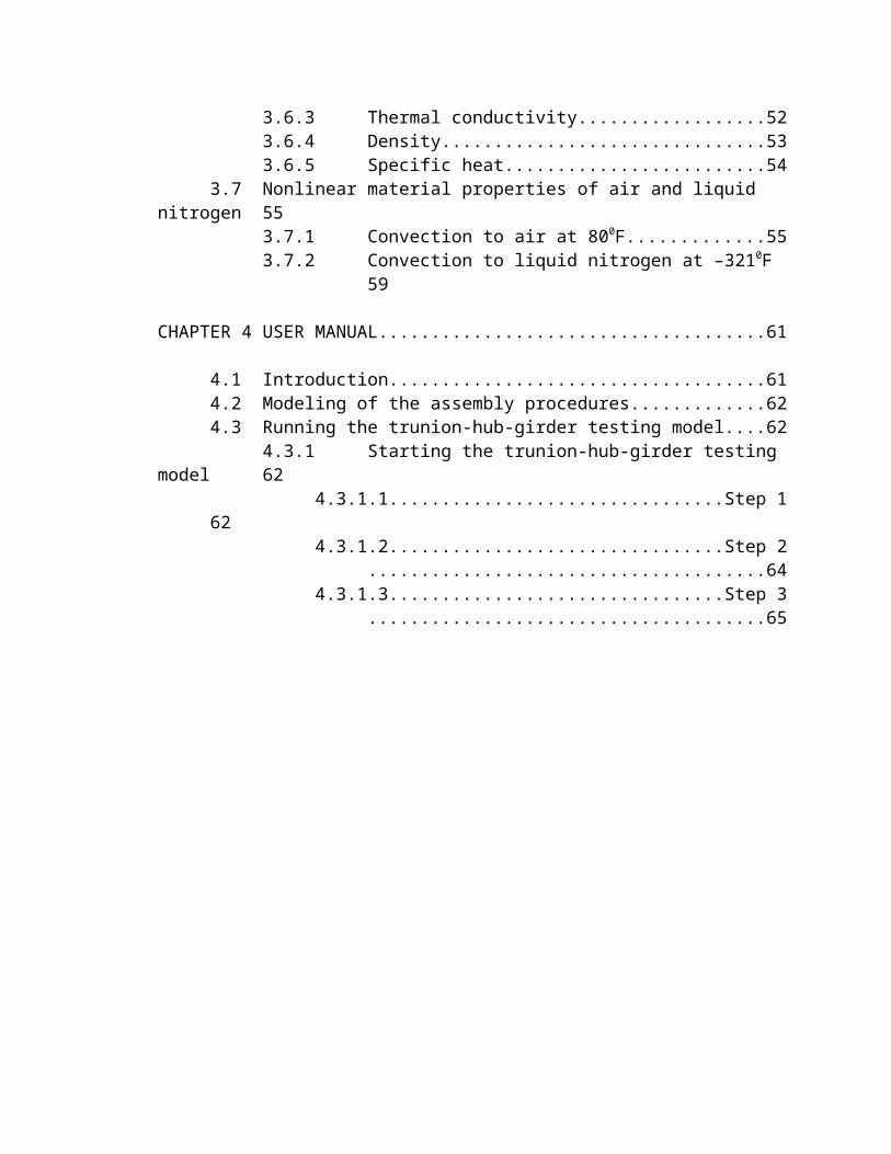
3.6 Nonlinear material properties of metal......................................................503.6.1 Young’s modulus...........................................................................503.6.2 Coefficient of thermal expansion...................................................513.6.3 Thermal conductivity.....................................................................523.6.4 Density...........................................................................................533.6.5 Specific heat...................................................................................54
3.7 Nonlinear material properties of air and liquid nitrogen...........................553.7.1 Convection to air at 800F...............................................................553.7.2 Convection to liquid nitrogen at –3210F........................................59
CHAPTER 4 USER MANUAL.......................................................................................61
4.1 Introduction................................................................................................614.2 Modeling of the assembly procedures.......................................................624.3 Running the trunion-hub-girder testing model..........................................62
4.3.1 Starting the trunion-hub-girder testing model................................624.3.1.1 Step 1.................................................................................624.3.1.2 Step 2.................................................................................644.3.1.3 Step 3.................................................................................65
4.3.2 Entering filenames.........................................................................664.3.2.1 Step 4.................................................................................664.3.2.2 Step 5.................................................................................664.3.2.3 Step 6.................................................................................674.3.2.4 Step 7.................................................................................674.3.2.5 Step 8.................................................................................684.3.2.6 Step 9.................................................................................69
4.3.3 Material and geometric parameters................................................704.3.3.1 Step 10...............................................................................704.3.3.2 Step 11...............................................................................714.3.3.3 Step 12 (choice=1).............................................................714.3.3.4 Step 12 (choice=2).............................................................72
4.3.3.4.1 Step 12a (choice=2)............................................724.3.3.4.2 Step 12b (choice=2)............................................744.3.3.4.3 Step 12c (choice=2)............................................77
4.3.4 Meshing input................................................................................784.3.4.1 Step 13...............................................................................784.3.4.2 Step 14...........................................................804.3.4.3 Step 15...............................................................................824.3.4.4 Step 16...............................................................................85
4.3.5 Loading input ................................................................................864.3.5.1 Step 17...............................................................................864.3.5.2 Step 18...............................................................................874.3.5.3 Step 19...............................................................................904.3.5.4 Step 20...............................................................................92
4.3.6 Trunnion-hub-girder testing model crash......................................954.4 Resuming an already saved job..................................................................96
4.4.1 Step 1.............................................................................................96
4.4.2 Step 2.............................................................................................97
4.4.3 Step 3.............................................................................................97
4.5 General postprocessor................................................................................974.5.1 Step 1.............................................................................................98
4.5.2 Step 2.............................................................................................98
4.5.3 Step 3.............................................................................................99
4.5.4 Plotting parts of the assembly......................................................1014.6 Time history postprocessor......................................................................101
4.6.1 Step 1...........................................................................................1024.6.2 Step 2...........................................................................................1024.6.3 Step 3a..........................................................................................1044.6.4 Step 3b.........................................................................................1054.6.5 Step 3c..........................................................................................1064.6.6 Step 3d.........................................................................................1074.6.7 Step 3e..........................................................................................1084.6.8 Options.........................................................................................110
CHAPTER 5 RESULTS AND CONCLUSIONS.........................................................111
5.1 Introduction..............................................................................................1115.2 Bridge geometric parameters...................................................................1125.3 Bridge loading parameters.......................................................................1135.4 Convergence test and result verification..................................................1145.5 Hoop stress, temperature and critical crack length..................................1155.6 Transient stresses and critical crack length using the trunion-hub-girder
testing model............................................................................................117
5.7 Christa McAuliffe bridge.........................................................................1185.7.1 Assembly procedure 1 (AP#1).....................................................118
5.7.1.1 Full assembly process......................................................1185.7.1.2 Cooling down of the trunnion..........................................1205.7.1.3 Sliding the trunnion into the hub.....................................1205.7.1.4 Cooling down the trunnion-hub assembly.......................1215.7.1.5 Sliding the trunnion-hub assembly into the girder...........125
5.7.2 Assembly procedure 2 (AP#2).....................................................1265.7.2.1 Full assembly process......................................................1265.7.2.2 Cooling down of the hub..................................................1275.7.2.3 Sliding the hub into the girder.........................................1305.7.2.4 Cooling down of the trunnion..........................................1305.7.2.5 Sliding the trunnion into the hub-girder assembly...........130
5.8 Hillsborough Avenue bridge....................................................................1325.8.1 Assembly procedure 1 (AP#1).....................................................132
5.8.1.1 Full assembly process......................................................1325.8.1.2 Cooling down of the trunnion].........................................1335.8.1.3 Sliding the trunnion into the hub.....................................1335.8.1.4 Cooling down the trunnnion-hub assembly.....................1345.8.1.5 Sliding the trunnion-hub assembly into the girder...........135
5.8.2 Assembly procedure 2 (AP#2).....................................................1365.8.2.1 Full assembly process......................................................1365.8.2.2 Cooling down the hub......................................................1375.8.2.3 Sliding the hub into the girder.........................................1385.8.2.4 Cooling down of the trunnion..........................................1395.8.2.5 Sliding the trunnion into the hub-girder...........................139
5.9 17th Street Causeway................................................................................1405.9.1 Assembly procedure 1 (AP#1).....................................................141
5.9.1.1 Full assembly process......................................................1415.9.1.2 Cooling down of the trunnion..........................................1425.9.1.3 Sliding the trunnion into the hub.....................................1425.9.1.4 Cooling down the trunnion-hub assembly.......................1435.9.1.5 Sliding the trunnion-hub assembly into the girder...........144
5.9.2 Assembly procedure 2 (AP#2).....................................................1455.9.2.1 Full assembly process......................................................1455.9.2.2 Cooling down of the hub..................................................146
5.9.2.3 Sliding the hub into the girder.........................................1475.9.2.4 Cooling down of the trunnion..........................................1485.9.2.5 Sliding the trunnion into the hub-girder assembly...........148
5.10 Comparison..............................................................................................1495.11 Crack arrest..............................................................................................1505.12 Possibility of failure during the insertion process and gap conduction.. .1535.13 Conclusions and recommendations..........................................................154
REFERENCES................................................................................................................156
LIST OF TABLES
Table 3.1 Element characteristics. 45
Table 5.1a Geometric parameters. 113
Table 5.1b Interference values. 113
Table 5.2 Bulk parameters. 113
Table 5.3a Results with different mesh densities. 114
Table 5.3b Comparison between trunnion-hub-girder testing model and bascule bridge design tools.
115
Table 5.4 Time for each step of AP#1 for the Christa McAuliffe Bridge. 119
Table 5.5 Time for each step of AP#2 for the Christa McAuliffe Bridge. 126
Table 5.6 Time for each step of AP#1 for the Hillsborough Avenue Bridge.
133
Table 5.7 Time for each step of AP#2 for the Hillsborough Avenue Bridge.
137
Table 5.8 Time for each step of AP#1 for the 17th Street Causeway Bridge.
142
Table 5.9 Time for each step of AP#2 for the 17th Street Causeway Bridge assembly procedures and different bridges.
146
Table 5.10 Minimum critical crack length and maximum hoop stress for different assembly procedures and different bridges.
149
LIST OF FIGURES
Figure 1.1 Trunnion-hub-girder (THG) assembly. 1
Figure 2.1a Trunnion coordinates (side view). 10
Figure 2.1b Trunnion coordinates (front view). 10
Figure 2.2a Hub coordinates (side view). 11
Figure 2.2b Hub coordinates (front view). 11
Figure 2.3a Girder coordinates (side view). 12
Figure 2.3b Girder coordinates (front view). 12
Figure 3.1 Modeling approach. 38
Figure 3.2a Thermal element SOLID70 and Structural element SOLID45.
46
Figure 3.2b Thermal element SHELL57 and Structural element SHELL63.
46
Figure 3.2c Contact elements CONTACT174 and TARGET170. 47
Figure 3.2d COMBIN37 element. 47
Figure 3.3 Young’s modulus of steel as a function of temperature. 51
Figure 3.4 Coefficient of thermal expansion of steel as a function of temperature.
52
Figure 3.5 Thermal conductivity of steel as a function of temperature.
53
Figure 3.6 Density of steel as a function of temperature. 53
Figure 3.7 Specific heat of steel as a function of temperature. 54
Figure 3.8a Volume coefficient of thermal expansion of air as a function of temperature.
55
Figure 3.8b Thermal conductivity of air as a function of temperature. 56
Figure 3.8c Kinematic viscosity of air as a function of temperature. 56
Figure 3.8 d Specific heat of air as a function of temperature. 57
Figure 3.8e Absolute viscosity of air as a function of temperature. 57
Figure 3.8f Mass density of air as a function of temperature. 58
Figure 3.8g Convective heat transfer coefficient of air as a function of temperature.
58
Figure 3.9 Convective heat transfer coefficient of liquid nitrogen as a function of temperature.
60
Figure 4.1 Interactive. 63
Figure 4.2 ANSYS windows. 65
Figure 4.3 ANSYS toolbar (assembly procedure). 65
Figure 4.4 Thermal filename. 66
Figure 4.5 Structural filename. 67
Figure 4.6a Trunnion cooling thermal filename. 67
Figure 4.6b Hub cooling thermal filename. 67
Figure 4.7a Trunnion cooling structural filename. 68
Figure 4.7b Hub cooling structural filename. 68
Figure 4.8a Trunnion-hub cooling thermal filename. 68
Figure 4.8b Trunnion cooling thermal filename. 69
Figure 4.9a Trunnion-hub cooling structural filename. 69
Figure 4.9b Trunnion cooling structural filename. 69
Figure 4.9c Error message. 70
Figure 4.10 Material choice menu. 70
Figure 4.11 Bridge options. 71
Figure 4.12 Bridge choices. 72
Figure 4.13a Trunnion dimensions. 73
Figure 4.13b Trunnion dimension parameters. 74
Figure 4.14a Hub dimensions. 75
Figure 4.14b Hub dimension parameters. 76
Figure 4.15a Girder dimensions. 77
Figure 4.15b Girder dimension parameters. 78
Figure 4.16a Girder divisions. 79
Figure 4.16b Girder division parameters. 79
Figure 4.17a Divisions along the length (trunnion). 80
Figure 4.17b Divisions along the length (hub). 81
Figure 4.17c Divisions along length parameters. 82
Figure 4.18a Trunnion radial and circumferential divisions. 83
Figure 4.18b Hub radial and circumferential divisions. 83
Figure 4.18c Girder radial and circumferential divisions. 84
Figure 4.18d Radial and circumferential division parameters. 85
Figure 4.19 Radial interference. 86
Figure 4.20 Applied thermal loads. 86
Figure 4.21a Time–temperature options (AP#1). 87
Figure 4.21b Time–temperature options (AP#2). 88
Figure 4.22a Ancillary cooling parameters (AP#1). 91
Figure 4.22b Ancillary cooling parameters (AP#2). 91
Figure 4.23a Fracture coefficients and constants. 93
Figure 4.23b ANSYS process status bar. 93
Figure 4.23c Task manager. 95
Figure 4.24 Enter filename. 96
Figure 4.25a ANSYS toolbar (set dimensions). 97
Figure 4.25b Re-dimensioning verification box. 97
Figure 4.26 Results summary. 98
Figure 4.27 Read results. 99
Figure 4.28a Plot results. 100
Figure 4.28b Contour plot. 100
Figure 4.29 ANSYS toolbar (choose part of interest). 101
Figure 4.30 ANSYS toolbar (time history postprocessor). 102
Figure 4.31a Enter part of interest. 102
Figure 4.31b Selected component. 103
Figure 4.31c Pick elements. 104
Figure 4.32 Pan- zoom-rotate. 105
Figure 4.33 Front view. 106
Figure 4.34 Right view. 107
Figure 4.35 Multiple entities. 107
Figure 4.36a Pick nodes. 108
Figure 4.36b Time history plot. 109
Figure 4.37a ANSYS toolbar (list results). 110
Figure 4.37b Time history listing. 110
Figure 5.1 Fracture toughness and temperature. 116
Figure 5.2 Front and side view of the chosen element in the Christa McAuliffe hub.
118
Figure 5.3 Critical parameters plotted against time (full assembly process during AP#1 of the Christa McAuliffe Bridge).
119

Figure 5.4 Critical parameters plotted against time (sliding the trunnion into the hub during AP#1 of the Christa McAuliffe Bridge).
120
Figure 5.5a Critical parameters plotted against time (cooling down of the trunnion-hub assembly during AP#1 of the Christa McAuliffe Bridge).
122
Figure 5.5b Hoop stress plot when the highest hoop stress during AP#1 is observed.
123
Figure 5.5c Temperature plot when the highest hoop stress during AP#1 is observed.
123
Figure 5.5d Hoop stress plot when the lowest critical crack length during AP#1 is observed.
124
Figure 5.5e Temperature plot when the lowest critical crack length during AP#1 is observed.
124
Figure 5.6 Critical parameters plotted against time (sliding the trunnion-hub assembly into the girder during AP#1 of the Christa McAuliffe Bridge).
125
Figure 5.7 Critical parameters plotted against time (full assembly process during AP#2 of the Christa McAuliffe Bridge).
126
Figure 5.8a Critical parameters plotted against time (cooling down of the hub during AP#2 of the Christa McAuliffe Bridge).
127
Figure 5.8b Hoop stress plot when the highest hoop stress during AP#2 is observed.
128
Figure 5.8c Temperature plot when the highest hoop stress during AP#2 is observed.
128
Figure 5.8d Hoop stress plot when the lowest critical crack length during AP#2 is observed.
129
Figure 5.8e Temperature plot when the lowest critical crack length during AP#2 is observed.
129
Figure 5.9 Critical parameters plotted against time (sliding the hub into the girder during AP#2 of the Christa McAuliffe Bridge).
130

Figure 5.10 Critical parameters plotted against time (sliding the trunnion into the hub-girder assembly during AP#2 of the Christa McAuliffe Bridge).
131
Figure 5.11 Front and side view of the chosen element in the Hillsborough Avenue hub.
132
Figure 5.12 Critical parameters plotted against time (full assembly process during AP#1 of the Hillsborough Avenue Bridge.
133
Figure 5.13 Critical parameters plotted against time (sliding of trunnion into the hub during AP#1 of the Hillsborough Avenue Bridge).
134
Figure 5.14 Critical parameters plotted against time (cooling down of the trunnion-hub assembly during AP#1 of the Hillsborough Avenue Bridge).
135
Figure 5.15 Critical parameters plotted against time (sliding the trunnion-hub assembly into the girder during AP#1 of the Hillsborough Avenue Bridge).
136
Figure 5.16 Critical parameters plotted against time (full assembly process during AP#2 of the Hillsborough Avenue Bridge).
137
Figure 5.17 Critical parameters plotted against time (cooling down of the hub during AP#2 of the Hillsborough Avenue Bridge).
138
Figure 5.18 Critical parameters plotted against time (sliding the hub into the girder during AP#2 of the Hillsborough Avenue Bridge).
139
Figure 5.19 Critical parameters plotted against time (sliding the trunnion into the hub-girder assembly during AP#2 of the Hillsborough Avenue Bridge).
140
Figure 5.20 Front and side view of the chosen element in the 17th Street Causeway hub.
141
Figure 5.21 Critical parameters plotted against time (full assembly process during AP#1 of the 17th Street Causeway Bridge).
142
Figure 5.22 Critical parameters plotted against time (sliding of trunnion into the hub during AP#1 of the 17th Street Causeway Bridge).
143
Figure 5.23 Critical parameters plotted against time (cooling down of the trunnion-hub assembly during AP#1 of the 17th Street Causeway).
144
Figure 5.24 Critical parameters plotted against time (sliding the trunnion-hub assembly into the girder during AP#1 of the 17th Street Causeway Bridge).
145
Figure 5.25 Critical parameters plotted against time (full assembly process during AP#2 of the 17th Street Causeway Bridge).
146
Figure 5.26 Critical parameters plotted against time (cooling down of the hub during AP#2 of the 17th Street Causeway Bridge).
147
Figure 5.27 Critical parameters plotted against time (sliding the hub into the girder during AP#2 of the 17th Street Causeway Bridge).
148
Figure 5.28 Critical parameters plotted against time (sliding the trunnion into the hub-girder assembly during AP#2 of the 17th Street Causeway Bridge).
149
Figure 5.29a and against temperature for A508 steel. 151
Figure 5.29b Critical parameters plotted against time (cooling down of the trunnion-hub assembly during AP#1 of the Hillsborough Avenue Bridge).
152
Figure 5.29c Critical parameters plotted against time (cooling down of the hub during AP#2 of the Hillsborough Avenue Bridge).
153
LIST OF SYMBOLS
crack length in
critical crack length in
hoop stress with infinite meshing psi
constant in convergence equation psi
specific heat at constant pressure BTU/(lb-ºF)
cdiv number of divisions in the circumferential direction for every 60º (between a pair of gussets)
nondimensional
coolt1 hub cooling time/trunnion cooling time min
coolt2 trunnion cooling time/trunnion-hub cooling time min
cool temperature factor nondimensional
hydraulic diameter in
Young’s modulus at absolute zero psi
temperature dependent Young’s modulus where i=1, 2, 3 represents the trunnion, the hub, and the girder, respectively
psi
Young’s modulus at a temperature psi
ex distance from the end of the backing ring to the end of the hub
in
exdiv number of divisions along the ex nondimensional
edge effect factor for stress intensity factor nondimensional
fdiv number of divisions along the length to the hub on the gusset side
nondimensional
acceleration due to gravity in/sec2
temperature dependent shear modulus, where i=1, 2, 3 represents the trunnion, the hub and the girder, respectively
psi
gfdiv number of divisions along the girder flange width nondimensional
Gr Grashof number nondimensional
temperature dependent convective heat transfer coefficient for cooling medium
BTU/(hr-ºF-in2)
heat transfer coefficient BTU/(hr-ºF-in2)
temperature dependent convective heat transfer coefficient for air
BTU/(hr-ºF-in2)
time at which user defined exit criteria are met in the hub during the cooling process
min
time at which the hub meets the user defined exit criteria min
time at which the interference between the hub and the girder is breached
min
time at which the interference between the hub and the girder is breached
min
hgf height of the girder flange in
hgfdiv number of divisions along the girder flange height nondimensional
hgw height of the girder in
warm temperature factor nondimensional
warm temperature factor nondimensional
time at which the hub meets the user defined exit criteria min
thermal conductivity BTU/(hr-in-ºF)
temperature dependent thermal conductivity, where i=1, 2, 3 represents the trunnion, the hub and the girder, respectively
BTU/(hr-in-ºF)
temperature-dependent critical crack arrest factor ksi-in1/2
temperature-dependent critical stress intensity factor ksi-in1/2
l extension of the trunnion on the gusset side (length to hub on the gusset side of the trunnion)
in
trunnion end coordinate in
hub end coordinate in
girder-hub contact end coordinate in
trunnion start coordinate in
hub start coordinate in
girder-hub contact end coordinate in
ldiv number of divisions along the length to the hub on the nondimensional
xvi

backing ring side
lf distance to hub flange in
lfdiv number of divisions along lf nondimensional
lg width of the girder in
lh total length of hub in
lt total length of trunnion in
myref reference strain temperature ºF
number of elements in the THG assembly nondimensional
Nu Nusselt number nondimensional
numdiv number of divisions in the radial direction in each of the trunnion, the hub and the girder
nondimensional
Pr Prandtl number nondimensional
radial coordinate in
trunnion inner radial coordinate in
hub inner radial coordinate in
girder inner radial coordinate in
trunnion outer radial coordinate in
hub outer radial coordinate in
hoop stress at a point with elements psi
rhg outer radius of the hub(minus flange) in
rho outer radius of the hub flange in
rti inner radius of the trunnion in
rto inner radius of the hub in
S constant used in equation for Young’s modulus psi
time after contact min
time before contact min
total time (cooling) min
total time (warming) min
ambient air temperature ºF
cooling medium bulk temperature ºF
xvii
Einstein characteristic temperature ºF
wall temperature ºF
cold temperature criterion ºF
warm temperature criterion ºF
ambient temperature ºF
time at which the user defined exit criteria are met in the trunnion during the cooling process
min
tg gusset thickness in
time at which the trunnion-hub assembly meets the user defined exit criteria during the cooling process
min
time at which the conduction between the trunnion and the hub is switched to “on”
min
time at which the interference between the trunnion and the hub is breached
min
time at which the trunnion-hub-girder assembly meets user defined exit criteria during the fitting of the trunnion-hub assembly into the girder
min
tinc time increments (warming) during AP#1 min
tincc time increments (cooling) during AP#1 min
tinc2 time increments (warming) during AP#2 min
tincc2 time increments (cooling) during AP#2 min
time at which the trunnion-hub assembly meets the user defined exit criteria
min
time at which the trunnion-hub-girder assembly meets user defined exit criteria during the fitting of the trunnion into the hub-girder assembly
min
ambient air bulk temperature ºF
cooling medium bulk temperature ºF
radial displacement, where i=1, 2, 3 represents the trunnion, the hub and the girder, respectively
in
axial displacement, where i=1, 2, 3 represents the trunnion, the hub and the girder, respectively
in
hoop displacement, where i=1, 2, 3 represents the trunnion, the hub and the girder, respectively
in
wbr backing ring width in
wbrdiv number of divisions along wbr nondimensional
xviii
wgf width of the flange of the girder in
wgw width of the girder in
wgwdiv number of divisions along wgw nondimensional
whf width of the hub flange in
whfdiv number of divisions along whf nondimensional
x-coordinate of girder flange on the left side as viewed from the gusset side of the THG assembly
in
x-coordinate of girder flange on the right side as viewed from the gusset side of the THG assembly
in
inner y-coordinate of girder flange (bottom) in
inner y-coordinate of girder flange (top) in
outer y-coordinate of girder flange (bottom) in
outer y-coordinate of girder flange (top) in
z-coordinate of girder flange on backing ring side in
constant in convergence equation nondimensional
volume coefficient of thermal expansion m3/m3/ºF
shear strain in r plane, where i=1, 2, 3 represents the trunnion, the hub and the girder, respectively
nondimensional
shear strain in rz plane, where i=1, 2, 3 represents the trunnion, the hub and the girder, respectively
nondimensional
shear strain in the z plane, where i=1, 2, 3 represents the trunnion, the hub and the girder, respectively
nondimensional
electronic contribution BTU/(lb-ºF2)
radial strain, where i=1, 2, 3 represents the trunnion, the hub and the girder, respectively
nondimensional
hoop strain, where i=1, 2, 3 represents the trunnion, the hub and the girder, respectively
nondimensional
axial strain, where i=1, 2, 3 represents the trunnion, the hub and the girder, respectively
nondimensional
absolute viscosity lb/(in-hr)
density lb/in3
radial stress, where i=1, 2, 3 represents the trunnion, the hub and the girder, respectively
psi
xix
radial stress psi
axial stress, where i=1, 2, 3 represents the trunnion, the hub and the girder, respectively
psi
axial stress psi
hoop stress psi
hoop stress where i=1, 2, 3 represents the trunnion, the hub and the girder
psi
shear stress in r plane, where i=1, 2, 3 represents the trunnion, the hub and the girder, respectively
psi
shear stress in rz plane, where i=1, 2, 3 represents the trunnion, the hub and the girder, respectively
psi
shear stress in z plane, where i=1, 2, 3 represents the trunnion, the hub and the girder, respectively
psi
kinematic viscosity in2-hr
Poisson’s ratio, where i=1, 2, 3 represents the trunnion, the hub and the girder, respectively
nondimensional
xx
PARAMETRIC FINITE ELEMENT MODELING OF TRUNNION HUB GIRDER
ASSEMBLIES FOR BASCULE BRIDGES
by
BADRI RATNAM
An Abstract
of a thesis submitted in partial fulfillmentof the requirements for the degree of
Master of Science in Mechanical EngineeringDepartment of Mechanical Engineering
College of EngineeringUniversity of South Florida
December 2000
Co-Major Professor: Glen H. Besterfield, Ph.D.Co-Major Professor: Autar K. Kaw, Ph.D.
xxi
Failures during fabrication of trunnion-hub-girder (THG) assemblies of bascule
bridges result in losses of hundreds of thousands of dollars every year. Crack formation
in the hub of the Miami Avenue Bridge, Christa McAuliffe Bridge and Brickell Avenue
Bridge during assembly led the Florida Department of Transportation (FDOT)to
commission a project to perform a complete numerical and experimental study to
investigate why the assemblies failed. This work is one part of the above project. In this
study, a numerical modeling of the different assembly procedures of the THG assembly is
developed.
A preliminary study of the steady state stresses using the Bascule Bridge Design
Tools revealed that the stresses are well below the ultimate tensile strength of the material
and could not have caused failure. This called for a further investigation of the transient
stresses developed during the assembly process.
Two assembly procedures exist for the assembly of trunnion-hub-girder
assemblies. The first (present) assembly procedure involves shrink-fitting the trunnion
into the hub and subsequently shrink-fitting the trunnion-hub assembly into the girder. A
second (alternative) assembly procedure involves shrink-fitting the hub into the girder
and shrink-fitting the trunnion into the hub-girder assembly. Our hypothesis is that the
hoop stress, temperature and fracture toughness are not optimized in the first assembly
procedure and the second assembly procedure may resolve this problem.
A parametric finite element model is designed in ANSYS called the Trunnion-
Hub-Girder Testing Model (THGTM) to analyze the stresses, temperatures and critical
crack lengths in the THG assembly during the two assembly procedures.
xxii
Small cracks present in the assembly propagate catastrophically once the crack
size exceeds the critical crack length. The THGTM is used to compare the hoop stress
and critical crack lengths during the two assembly procedures for different bridges. The
critical points in the assembly and the critical stages during the two assembly process are
identified based on the critical crack length. The benefits of one assembly procedure
over another is assessed and recommendations to prevent crack formation in future
assemblies are presented.
Abstract Approved: Co-Major Professor: Glen H. Besterfield, Ph.DAssociate Professor, Department of Mechanical Engineering
Date Approved:_______________________________________
Co-Major Professor: Autar K. Kaw, Ph.DProfessor, Department of Mechanical Engineering
Date Approved:_______________________________________
xxiii

CHAPTER 1
BACKGROUND
1.1 Introduction
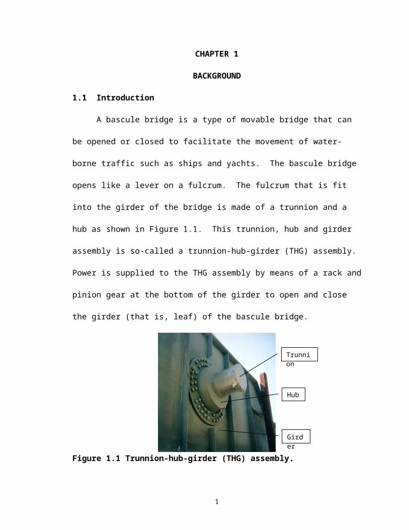
A bascule bridge is a type of movable bridge that can be opened or closed to
facilitate the movement of water-borne traffic such as ships and yachts. The bascule
bridge opens like a lever on a fulcrum. The fulcrum that is fit into the girder of the bridge
is made of a trunnion and a hub as shown in Figure 1.1. This trunnion, hub and girder
assembly is so-called a trunnion-hub-girder (THG) assembly. Power is supplied to the
THG assembly by means of a rack and pinion gear at the bottom of the girder to open and
close the girder (that is, leaf) of the bascule bridge.
Figure 1.1 Trunnion-hub-girder (THG) assembly.
The THG assembly is generally made by interference fits between the trunnion
and hub, and the hub and girder. Typical interference fits used in the THG assemblies in
Florida bascule bridges are FN2 and FN3 fits.
FN2 and FN3 fits are US standard based fits used in light and medium drives,
respectively. According to Shigley and Mischke (1986b) FN2 designation is as follows
“Medium-drive fits are suitable for ordinary steel parts or for shrink fits on light sections.
1
Trunnion
Hub
Girder
They are about the tightest fits that can be used with high-grade cast-iron external
members.” Furthermore, FN3 designation is “Heavy drive fits are suitable for heavier
steel parts or for shrink fits in medium sections”.
The current assembly procedure used throughout Florida works as follows.
1. The trunnion is cooled in liquid nitrogen, allowing it to be shrink-fitted into the
hub.
2. The trunnion is then inserted into the hub and allowed to warm up to ambient
temperature to develop an interference fit with the hub.
3. The resulting trunnion-hub assembly is then cooled in liquid nitrogen, allowing it
to be shrink-fitted into the girder.
4. The trunnion-hub-girder assembly is then inserted into the girder and allowed to
warm up to ambient temperature to develop interference fits between the trunnion
and the hub, and the hub and the girder.
On May 3rd, 1995 during the immersion of the trunnion-hub assembly in liquid
nitrogen (that is, Step3 above) for the Christa McAuliffe Bridge in Brevard County, FL, a
cracking sound was heard in the trunnion-hub assembly. On removing the trunnion-hub
assembly out of liquid nitrogen, it was found that the hub had cracked near its inner
radius. In a separate instance, during the assembly of the Venetian Causeway Bascule
Bridge, while inserting the trunnion into the hub, the trunion stuck in the hub before
complete insertion took place. A possible cause of difficulties in this instance is the
trunnion not shrinking enough in the dry ice/alcohol cooling medium.
Mindful of the losses caused by the failures and eager to prevent their recurrence
the Florida Department of Transportation decided to investigate the cause of failure in the
2
THG assemblies. Some questions by the FDOT were as follows. Why were these
failures taking place and only on a few of the many THG assemblies carried out in
Florida? Why were they not happening on the same THG assemblies again? How can
we avoid losses of hundreds of thousands dollars in material, labor and delay in replacing
the cracked assemblies? Preliminary investigations done by independent consulting firms
and the assembly manufacturers gave various reasons for the possible failure including
high cooling rate, use of liquid nitrogen as a cooling medium, residual stresses in the
castings and the assembly procedure itself.
FDOT officials wanted to carry out a complete numerical and experimental study
to find out why the assemblies failed, how they could be avoided in the future and to
develop clear specifications for the assembly procedure. So, in 1998, they gave a two-
year $250,000 grant to the College of Engineering at the University of South Florida to
investigate the problem.
The first study conducted for the grant by Denninger (2000) to find steady state
stresses in the THG assembly showed that these stresses are well below the ultimate
tensile strength (UTS) of the materials used in the assembly. Hence, these stresses could
not have caused the failure. The results called for an investigation of the transient tresses
during the assembly process. The stresses during the assembly process came from two
sources – thermal stresses due to temperature gradients and mechanical stresses due to
interference at the trunnion-hub and hub-girder interfaces. Are these transient stresses
more than the allowable stresses? Since fracture toughness values decrease with a
decrease in temperature, do these transient stresses make the assembly prone to fracture?
These are some of the questions to be answered.
3
At the outset, it became apparent that isolating and pinpointing the causes of
failure intuitively is difficult for three reasons. First, it was observed that cracks were
formed in some bridge assemblies but not in others. Second, the cracks occurred in
different parts of the hub for different bridges and at different loading times. Last, the
problem involves an interplay of several issues, that is,
1. Complex geometries, such as, gussets on the hub, make it a 3-D elasticity and
heat transfer problem.
2. Thermal-structural interaction, due to the cooling and warming of the THG
components and the shrink fitting of these components, results in both thermal
and mechanical stresses. In addition, conduction takes place along contact
surfaces.
3. Temperature-dependent material properties, such as, coefficient of thermal
expansion, specific heat, thermal conductivity, ultimate tensile strength and
fracture toughness, can be highly nonlinear functions of temperature.
Hence, an intuitive analysis is not merely difficult but intractable.
The aim of this study is to build a finite element model in ANSYS to evaluate
THG assemblies for transient thermal and interference stresses during fabrication. The
model is used to investigate the reasons for the crack formation in existing assemblies
and design new assemblies in the future that do not form cracks. The finite element
approach is most suitable because it can handle the interplay of complex geometries,
coupled thermal and structural fields, and temperature dependent properties.
ANSYS was chosen as the Finite Element Method (FEM) software of choice
principally because of its strength in thermo-structural analysis. Also, the twin ANSYS
4
languages ANSYS parametric design language (APDL) and User interface design
language (UIDL) allow us to develop user friendly interfaces that can be used by a design
engineer.
The existing assembly procedure, henceforth called AP#1, involves shrink fitting
the trunnion into the hub and subsequently shrink fitting the trunnion-hub assembly into
the girder. Our hypothesis is that the hoop stresses and proneness to fracture are not
optimized in the existing assembly procedure. An alternative, possibly better, assembly
procedure, henceforth called AP#2, involves shrink fitting the hub into the girder and
subsequently shrink fitting the trunnion into the hub-girder assembly. Using a parametric
model, transient stresses in the two alternative assembly procedures for different bridges
are compared and our hypothesis is tested using time-history plots of temperature and
stress.
The model, as the name suggests, is parametric allowing the user to modify
geometries, material and thermal properties of assembly materials and convective media,
interference values, temperature of cooling and ambient convective media, and loading
times. Also, depending on the required degree of accuracy, the user can also change
mesh density and time steps. Options for different THG assemblies and different
assembly procedures are included in the model. The results, such as, temperature and
stress, are displayed both as a function of position (time fixed) in contour plots and as a
function of time (position fixed).
The principal aims while making the model were to make it simple and user-
friendly. However, in our quest for brevity and simplicity, care was taken not to
compromise the more important goals of accuracy and flexibility. Some rudimentary
5
knowledge of finite element modeling as regards to element shape testing, costs of mesh
refinement, efficiency of computational time, accuracy trade-off, thermal-structural field
interaction, limitations and assumptions of the model are expected of the user.
1.2 History
This study is primarily focused on analyzing transient stresses and failures caused
due to them. This broad scope encompasses topics such as temperature-dependent
material properties, thermoelastic contact, thermal shock and fracture toughness. A brief
history of previous work done in these areas and the relevance of each to this study is
explained. Also, a justification for this study because of the limitations of the previous
research efforts and unique requirements of this project is included.
Pourmohamadian and Sabbaghian (1985) modeled the transient stresses in a solid
cylinder with temperature dependent material properties under an axisymmetric load.
However, their model does not incorporate non-symmetric loading, complex geometries
and thermoelastic contact, all of which are present in the THG assembly.
The trunnion-hub interface and the hub-girder interface are in thermoelastic
contact. Attempts were made to model thermoelastic contact between twin cylinders by
Noda (1985). However, the models were only applicable for cylinders and not for non-
standard geometries. Also, the issue of temperature-dependent material properties was
not addressed in this study.
Takeuti and Noda (1980) studied transient stresses in a cylinder under
nonaxisymmetric temperature distribution. This study is relevant to our research efforts
due to complex geometry and temperature-dependent material properties of the THG
assembly and being under nonaxisymmetric temperature distribution. However, the
6
issues of thermoelastic contact and complex geometries are not addressed in this study.
Noda also modeled a transient thermoelastic contact problem with a position dependent
heat transfer coefficient (1987) and transient thermoelastic stresses in a short length
cylinder (1985). These efforts, although useful to understanding the thermoelastic
modeling, did not address the issues of temperature dependent material properties and
complex geometries.
Enumerated below are studies that aided us in the understanding the role of
fracture toughness in the study. Thomas, et al. (1985) found the thermal stresses due to
the sudden cooling of cylinder after heating due to convection. The results indicated the
magnitude of stresses attained during the cooling phase increases with increasing
duration of heating. Consequently, the duration of application of the convective load can
be a factor influencing the maximum stresses attained in the assembly.
Parts of the THG assembly are subjected to thermal shock when they are cooled
down before shrink fitting. Oliveira and Wu (1987) determined the fracture toughness
for hollow cylinders subjected to stress gradients arising due to thermal shock. The
results covered a wide range of cylinder geometries.
It is clear that the drawback of all previous studies of transient thermal stresses is
their inability to deal with non-standard geometries. In addition, previous research efforts
address some of the issues (for example, temperature dependent material properties,
thermoelastic contact, nonaxisymmetric loading, and thermal shock) but never all of the
issues. Our research efforts are concentrated less on isolating the effects of individual
factors affecting the stresses in the THG assembly than on observing the interplay of
7
assorted factors acting together. Hence, this study breaks new ground in the study of
thermal stresses.
1.3 Overview
Chapter 2 describes the mathematical and engineering aspects of the problem.
Details of the THG assembly dimensions, assembly procedures and boundary conditions
are covered in this chapter. In Chapter 3, the modeling approach and assumptions used in
the model are explained. Particular emphasis is given to the interaction between the
thermal and structural fields. The nonlinear material properties of the steel used in the
THG assembly, and the thermal properties of air and liquid nitrogen are plotted are
plotted in Chapter 3. In Chapter 4, a technical manual is presented to show how a design
engineer can use the ANSYS software to find transient stresses for any existing or new
THG assemblies. In Chapter 5, results are discussed for THG geometries of three bridges
(that is, Christa McAuliffe Bridge, 17th Street Causeway Bridge, and Hillsborough
Avenue Bridge) using both assembly procedures, AP#1 and AP#2. The temperature,
critical crack length and hoop stress are used as parameters for comparison between
different assembly procedures and different bridges. The conclusions and
recommendations of this study are also presented in Chapter 5.
8
CHAPTER 2
TECHNICAL DETAILS
2.1 Introduction
The technical and mathematical aspects of this study are described in this chapter.
The objective of this chapter is to define the scope, specifications and details of the
phenomena modeled in the parametric finite element model. The subsequent chapter
describes how these requirements are met. The existing assembly procedure, AP#1
results in crack formation in the hub of some of the bridges. An alternative assembly
procedure, AP#2 is suggested which can possibly rectify some, if not all the problems
associated with the earlier assembly procedure. The thermal and structural boundary
conditions on the trunnion-hub-girder assembly during different steps in the two
assembly procedures are presented.
2.2 Geometry of the trunnion-hub-girder assembly
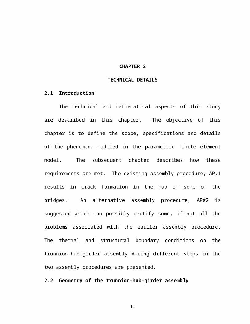
Figures 2.1a and 2.1b, 2.2a and 2.2b, and 2.3a and 2.3b show the geometries of
the trunnion, hub and girder, respectively. The interference between the trunnion-hub
and the hub-girder is determined by the Bascule Bridge Design Tools (Denninger 2000)
for FN2 and FN3 fits.
9
Figure 2.1a Trunnion coordinates (side view).
Figure 2.1b Trunnion coordinates (front view).
10
1or
1ir
1el
2el
2sl
1sl
z
trunnion-hub contact surface
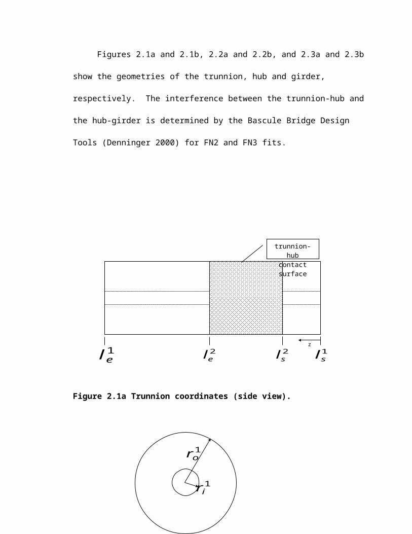
Figure 2.2a Hub coordinates (side view).
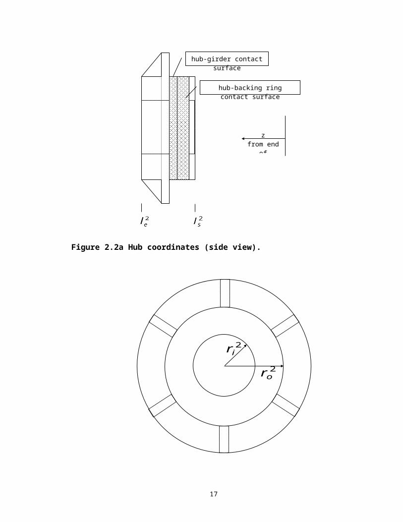
Figure 2.2b Hub coordinates (front view).
11
2ir
2or
zfrom end of
trunnion
hub-girder contact surface
hub-backing ring contact surface

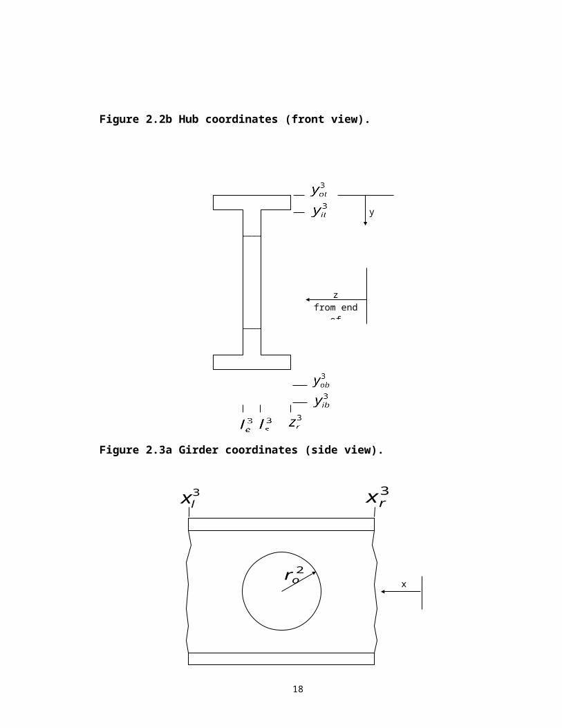
Figure 2.3a Girder coordinates (side view).
Figure 2.3b Girder coordinates (front view).
12
3rx
x2
or
3lx
y
zfrom end of
trunnion
2.3 Assembly procedures
Two assembly procedures are studied in this work.
2.3.1 Assembly procedure 1 (AP#1)
The present assembly procedure involves the following four steps.
1. Cooling down of the trunnion in a cooling medium.
2. Sliding the trunnion into the hub. Convection with ambient air results in a
warming of the trunion. This results in an interference fit between the trunnion
and hub, and then conduction between the trunion and the hub.
3. Cooling down the trunnion-hub assembly in a cooling medium.
4. Sliding the trunnion-hub assembly into the girder. Convection with the ambient
air results in a warming up of the trunnion-hub assembly. This results in an
interference fit between the trunnion-hub assembly and the girder, and conduction
between the trunnion-hub assembly and the girder.
2.3.2 Assembly procedure 2 (AP#2)
1. Cooling down of the hub in a cooling medium.
2. Sliding the hub into the girder. Convection with ambient air results in a warming
up of the hub. This results in an interference fit between hub and the girder, and
conduction between the hub and the girder.
3. Cooling down the trunnion in a cooling medium.
4. Sliding the trunnion into the hub-girder assembly. Convection with the ambient
air results in a warming up of the trunion. This results in an interference fit
between the trunnion, the hub-girder assembly, and conduction between the
trunion and the hub-girder assembly.
13
2.4 Equations of equilibrium, strain displacement equations and stress-strain equations
To develop the equations of equilibrium, the following symbols are used, where
i=1, 2, 3 represent the trunnion, hub and girder, respectively.
= radial stress
= hoop stress
= axial stress
= shear stress in r plane
= radial strain
= hoop strain
= axial strain
= radial displacement
= hoop displacement
= axial displacement
= shear strain in the r plane
= shear strain in the z plane
= shear strain in the rz plane
= temperature dependent Poisson’s ratio
= temperature dependent thermal conductivity
= temperature dependent shear modulus
= temperature dependent heat transfer coefficient of cooling meduim
= temperature dependent heat transfer coefficient of warming meduim
14
The equations of equilibrium and compatibility for the trunnion-hub and girder
are presented next (Ugural and Fenster, 1995).
2.4.1 Equations of equilibrium
, (2.1a)
, (2.1b)
=0, (2.1c)
where i=1, 2, 3 represent the trunnion, hub and the girder, respectively.
2.4.2 Stress-strain equations
, (2.2a)
, (2.2b)
, (2.2c)
, (2.2d)
, (2.2e)
, (2.2f)
where i=1, 2, 3 represent the trunnion, the hub and the girder, respectively.
2.4.3 Strain displacement equations
15
, (2.3a)
, (2.3b)
, (2.3c)
, (2.3d)
, (2.3e)
, (2.3f)
where i=1, 2, 3 represent the trunnion, the hub and the girder, respectively.
2.5 Boundary conditions on the trunnion-hub-girder assembly
The boundary conditions on the THG assembly at the various steps during the two
assembly procedures are presented next. Because of the complexity of the geometry,
boundary conditions are given only at the surfaces of contact (before and after contact)
and those imposed for limiting rigid body motions in the finite element analysis. Areas
for which the boundary conditions are not specified are stress free.
2.5.1 Assembly procedure (AP #1)
2.5.1.1 Cooling down of the trunnion
The trunnion is dipped in a cooling medium that has a temperature, and kept in
the medium until it nears steady state after units of time. The thermal boundary
conditions are discussed next. At the inner radius, , of the trunnion,
, , , , (2.4a)
16
and at the outer radius, , of the trunnion,
, , , . (2.4b)
The structural boundary conditions are the following. At the inner radius, , of the
trunnion,
, , , , (2.4c)
, , , , (2.4d)
and the outer radius, , of the trunnion,
, , , , (2.4e)
, , , .(2.4f)
At the right edge of the trunnion at , the trunnion is constrained as
, , , , (2.4g)
, , , , (2.4h)
, , , . (2.4i)
2.5.1.2 Sliding the trunnion into the hub
After immersion in a cooling medium, the trunnion is expanded by convection
with the ambient air at a temperature, . The trunnion expands for units of time
before it comes into contact with the hub. After contact, the trunnion-hub assembly nears
steady state after units of time. The total trunnion warming time is given by
. (2.5a)
Before contact, the thermal boundary conditions at the inner radius, , of the trunnion
are
17
, , , , (2.5b)
and at the outer radius, , of the trunnion,
, , , . (2.5c)
After contact, the thermal boundary conditions at the inner radius, , of the trunnion
are
, , , , (2.5d)
and at the outer radius of the trunnion, are the following. For the surfaces not in
contact,
, , , , ,
(2.5e)
and for the surfaces in contact,
, , , . (2.5f)
The structural boundary conditions on the trunnion and the hub are the following.
Before contact, the structural boundary conditions on the trunnion are as given next. At
the inner radius, , of the trunnion,
, , , , (2.5g)
, , , , (2.5h)
and at the outer radius, , of the trunnion,
, , , , (2.5i)
18
, , , . (2.5j)
At the right edge of the trunnion at, , the trunnion is constrained by
, , , , (2.5k)
, , , , (2.5l)
, , , , (2.5m)
and at the inner radius, , of the hub,
, , , , (2.5n)
, , , , (2.5o)
and at the outer radius, , of the hub,
, , , , (2.5p)
, , , . (2.5q)
After contact, the following structural boundary conditions hold. At the inner radius of
the trunnion, ,
, , , , (2.5r)
, , , , (2.5s)
and at the outer radius of the trunnion, , where there is no contact,
, , , , ,
(2.5t)
, , , , .
19
(2.5u)
At the right edge of the trunnion at, , the trunnion is constrained with the following
boundary condition
, , , , (2.5v)
, , , , (2.5w)
, , , , (2.5x)
and at the surface in contact at the trunnion outer radius, ,
, , , , (2.5y)
, , , , (2.5z)
, , , , (2.5aa)
, , , . (2.5bb)
At the outer radius of the hub, ,
, , , , (2.5cc)
, , , (2.5dd)
and at the right edge, , of the hub the following constraint exists
, , , , (2.5ee)
, , , . (2.5ff)
20
2.5.1.3 Cooling down of the trunnion-hub assembly
The trunnion-hub assembly is immersed in a cooling medium at temperature, ,
until it nears steady state at time . The thermal boundary conditions at the inner radius
of the trunnion, , is
, , , . (2.6a)
At the outer radius of the trunnion, , there are non-contact and contact surfaces. At
the non-contact surface
, , , , ,
(2.6b)
and at the contact surface,
, , , . (2.6c)
The structural boundary conditions are on the inner radius, , of the trunnion are
, , , , (2.6d)
, , , , (2.6e)
At the outer radius of the trunnion, , where there is no contact, the boundary
conditions are
, , , , ,
(2.6f)
, , , , ,
(2.6g)
21
and at the surface in contact at the trunnion outer radius, ,
, , , , (2.6h)
, , , , (2.6i)
, , , , (2.6j)
, , , . (2.6k)
At the right edge of the trunnion at , the trunnion is subjected to
, , , , (2.6l)
, , , , (2.6m)
, , , . (2.6n)
At the outer radius, , of the hub,
, , , , (2.6o)
, , , ,(2.6p)
and the right edge, , of the hub is constrained with the following boundary
conditions
, , , , (2.6q)
, , , , (2.6r)
, , , . (2.6s)
2.5.1.4 Sliding the trunnion-hub assembly into the girder
After immersion in the cooling medium the trunnion-hub assembly is expanded
by convection with the ambient air at temperature . The trunnion hub assembly
expands for units of time before it comes into contact with the girder. After contact
22
the THG assembly nears steady state after units of time. The total warming time is
then given by
. (2.7a)
The thermal boundary conditions before contact at the inner radius, , of the trunnion
are
, , , , (2.7b)
and the boundary conditions at the outer radius, , of the trunnion, at the non-contact
surface are
, , , , .
(2.7c)
At the outer radius, , of the trunnion, at the contact surface,
, , , , (2.7d)
and at the hub outer radius, , of the hub,
, , , . (2.7e)
After contact, at the inner radius, , of trunnion,
, , , , (2.7f)
and at the outer radius, , of the trunnion, at the non-contact surface,
, , , , ,
(2.7g)
23
At the outer radius, , of the trunnion, at the contact surface,
, , , , (2.7h)
and at the outer radius, , of the hub, at the non-contact surface,
, , , , ,
(2.7i)
and at the outer radius, , of the hub, at the contact surface,
, , , . (2.7j)
The structural boundary conditions for this step of the assembly procedure are as follows.
Before contact, on the inner radius, , of the trunnion, the boundary conditions are
, , , , (2.7k)
, , , , (2.7l)
and at the outer radius of the trunnion, , where there is no contact,
, , , ,
(2.7m)
, , , .
(2.7n)
At the surface in contact at the trunnion outer radius, ,
, , , (2.7o)
, , , (2.7p)
24
, , , (2.7q)
, , . (2.7r)
At the outer radius, , of the hub,
, , , (2.7s)
, , .(2.7t)
At the right edge of the trunnion at, , the trunnion is subjected to following
constraints
, , , , (2.7u)
, , , , (2.7v)
, , , . (2.7w)
After contact, at the inner radius, , of the trunnion,
, , , , (2.7x)
, , , , (2.7y)
and at the outer radius, , of the trunnion, at the non-contact surface,
, , , , (2.7z)
, , , . (2.7aa)
At the outer radius, , of the trunnion, at the contact surface,
, , , , (2.7bb)
, , , , (2.7cc)
25
, , , , (2.7dd)
, , , , (2.7ee)
and at the outer radius, of the hub, at the non-contact surface,
, , , ,
(2.7ff)
, , , , .
(2.7gg)
At the outer radius, of the hub, at the contact surface,
, , , , (2.7hh)
, , , , (2.7ii)
, , , , (2.7jj)
, , , . (2.7kk)
The right edge, , of the hub is constrained, with the following boundary conditions
, , , , (2.7ll)
, , , . (2.7mm)
At the inner radius, , of the girder,
, , , , (2.7nn)
, , , . (2.7oo)
26
On the outer edge of the girder, the surfaces are stress free except for the following
constraints
=0, , , , .
(2.7pp)
2.5.2 Assembly Procedure 2 (AP#2)
2.5.2.1 Cooling down of the hub
The hub is dipped in the cooling medium with a temperature till it nears steady
state at units of time. The thermal boundary conditions are given by the following two
equations. At the inner radius, , of the hub
, , , , (2.8a)
and at the outer radius, , of the hub,
, , , . (2.8b)
The structural boundary conditions are the following. At the inner radius, , of the
hub,
, , , , (2.8c)
, , , , (2.8d)
and at the outer radius, , of the hub,
, , , , (2.8e)
, , , . (2.8f)
At the right edge, , of the hub,
27
, , , , (2.8g)
, , , , (2.8h)
, , , . (2.8i)
2.5.2.2 Sliding the hub into the girder
After immersion in a cooling medium the hub is expanded by convection with the
ambient air at a temperature . The hub expands for units of time before it comes
into contact with the girder. The hub-girder assembly nears steady state after units of
time. The total warming time is then given by
. (2.9a)
Before contact, the thermal boundary conditions at the inner radius, , of the hub is
, , , , (2.9b)
and at the outer radius, , of the hub,
, , , . (2.9c)
After contact, at the inner radius, , of the hub,
, , , , (2.9d)
and at the outer radius, , of the hub, for the surfaces not in contact,
, , , , ,
(2.9e)
and at the outer radius, , of the hub, for the surfaces in contact,
28
, , , . (2.9f)
The structural boundary conditions on the hub and the girder are given next. Before
contact, at the inner radius, , of the hub,
, , , , (2.9g)
, , , . (2.9h)
At the outer radius, , of the hub
, , , , (2.9i)
, , , . (2.9j)
After contact, the following boundary conditions hold. At the inner radius, , of the
hub,
, , , , (2.9k)
, , , . (2.9l)
At the outer radius, , where the surfaces are not in contact,
, , , , ,
(2.9m)
, , , , ,
(2.9n)
and at surfaces in contact at the outer radius, , of the hub,
29
, , , , (2.9o)
, , , , (2.9p)
, , , , (2.9q)
, , , . (2.9r)
At the right edge, , of the hub,
, , , , (2.9s)
, , , , (2.9t)
, , , . (2.9u)
On the outer of the girder, the surfaces are stress free except for the following constraints
=0, , , , .
(2.9v)
2.5.2.3 Cooling down of the trunnion
The trunnion is dipped in the cooling medium with a temperature till it nears
steady state after units of time. The thermal boundary conditions of the trunnion are
, , , , (2.10a)
at the inner radius, , and
, , , , (2.10b)
at outer radius, , of the trunnion. The structural boundary conditions on the inner
radius, , of the trunnion are
30

, , , , (2.10c)
, , , . (2.10d)
At the outer radius, , of the trunnion,
, , , , (2.10e)
, , , , (2.10f)
and at the right edge the trunnion at, , the trunnion is constrained, that is,
, , , , (2.10g)
, , , , (2.10h)
, , , . (2.10i)
2.5.2.4 Sliding the trunnion into the hub-girder assembly
After immersion in a cooling medium, the trunnion is expanded by convection
with the ambient air at a temperature . The trunnion expands for units of time
before it comes into contact with the hub. The trunnion-hub-girder assembly nears steady
state after units of time. The total time for warming is given by
. (2.11a)
Before contact, the thermal boundary conditons at the inner radius, , of the trunnion
are
, , , , (2.11b)
and at the outer radius, , of the trunnion,
, , , . (2.11c)
31
At the outer radius, , of the hub, for the surfaces not in contact,
, , , , ,
(2.11d)
and for the surfaces in contact,
, , , . (2.11e)
After contact, at the inner radius, , of the trunnion,
, , , . (2.11f)
At the outer radius, , of the trunnion, for the surfaces not in contact,
, , , , ,
(2.11g)
and for the surfaces in contact,
, , , . (2.11h)
At the outer radius, , of the hub, for the surfaces not in contact,
, , , ,
(2.11i)
and for surfaces in contact,
, , , . (2.11k)
32
The structural boundary conditions are as follows. Before contact, at the inner radius,
, of the trunnion,
, , , , (2.11l)
, , , . (2.11m)
At the outer radius, , of the trunnion,
, , , , (2.11n)
, , , , (2.11o)
and at the right edge of the trunnion at ,
, , , , (2.11p)
, , , . (2.11q)
At the inner radius, , of the hub, for the surfaces not in contact,
, , , , ,
(2.11r)
, , , , ,
(2.11s)
and for the surfaces in contact,
, , , , (2.11t)
, , , , (2.11u)
, , , , (2.11v)
, , , . (2.11w)
33

At the right edge, , of the hub,
, , , , (2.11x)
, , , . (2.11y)
After contact, at the inner radius, ,of the trunnion,
, , , , (2.11z)
, , , . (2.11aa)
At the outer radius of the trunnion, , for thesurfaces not in contact,
, , , , (2.11bb)
, , , , (2.11cc)
, , , , (2.11dd)
, , , , (2.11ee)
and for the surfaces in contact,
, , , , (2.11ff)
, , , , (2.11gg)
, , , , (2.11hh)
, , , . (2.11ii)
At the right edge the trunnion at , the trunnion is constrained with the following
boundary condition
34
, , , , (2.11jj)
, , , . (2.11kk)
, , , . (2.11ll)
At the outer radius, , of the hub, for the surfaces not in contact,
, , , , ,
(2.11mm)
, , , , ,
(2.11nn)
and for the surfaces in contact,
, , , , (2.11oo)
, , , , (2.11pp)
, , , , (2.11qq)
, , , . (2.11rr)
At the right edge, , of the hub,
, , , , (2.11ss)
, , , . (2.11tt)
, , , . (2.11uu)
The girder is contrained at the outer edge by
, , , , (2.11vv)
35
, , , . (2.11ww)
On the outer of the girder, the surfaces are stress free except for the following constraints
=0, , , ,
(2.11vv)
36
CHAPTER 3
NUMERICAL MODELING AND MATERIAL PROPERTIES
3.1 Introduction
An understanding of the modeling approach is necessary to appreciate the validity
of the results, inherent assumptions, and consequential limitations of the parametric
model. This chapter describes how the phenomena, requirements and boundary
conditions described in the previous chapter are incorporated into the parametric model.
Some problems associated with the Finite Element Modeling (FEM) of thermo-structural
analysis and their resolution using some non-conventional approaches are described.
Assumptions made in the model are justified based on the physics of the problem,
cost versus accuracy trade-off, limitations of finite element method, and need for
simplicity. Nonlinear material properties for steel, air, and liquid nitrogen are plotted at
the end of this chapter.
3.2 Coupled field analysis
Coupled field analysis involves an interaction of two or more types of
phenomena. This study involves the coupling of the thermal and structural fields.
ANSYS features two types of coupled field analysis.
3.2.1 Direct coupled field analysis
In direct coupled field analysis, degrees of freedom of multiple fields are
calculated simultaneously. This method is used when the responses of the two
phenomena are dependent upon each other, and is computationally more intensive.
37
3.2.2 Indirect coupled field (sequential coupled field analysis)
In this method, the results of one analysis are used as the loads of the following
analysis. This method is used where there is one-way interaction between the two fields.
3.3 Design of the model
The sequential coupled field method described above is chosen as the approach
best suited to our requirements. The underlying assumption is that the structural results
are dependent upon the thermal results, but not vice-versa. This assumption is valid for
the requirements of our study. Typically, this involves performing the entire thermal
analysis, and subsequently transferring the thermal nodal temperatures to the structural
analysis. However, our problem requires some modifications to the pure form of this
approach as interaction between the two fields (thermal and structural) is required to
determine the time of contact between parts of the assembly during the process of shrink-
fitting. This is achieved using a non-conventional approach.
First, the thermal analysis of the cooling down of part(s) to steady state is
performed. Subsequently, the structural analysis is performed to determine the time
when the interference between the two parts of the assembly is breached. These
parameters are used in the complete thermal analysis to switch thermal and structural
contact ‘on’ and ‘off’, that is, to determine whether conductance is taking place between
the parts of the assembly. The minimum temperature in the assembly during cooling
down and the maximum temperature during warming up process are monitored and the
program exits the process in question once it nears steady state. The modeling procedure
is described in the Figure 3.1.
38
Figure 3.1 Modeling approach.
39
In this model, we perform multiple thermal and structural analysis to determine
time parameters at which certain thermal and structural criteria are met. The thermal
results obtained are transferred as nodal temperatures to the structural analysis.
These parameters are used to perform the complete thermal and structural analysis
along with the ancillary cooling analyses. Segments of the flowchart shown in Figure 3.1
are explained next. The section headings explain the namesake process boxes in the
flowchart.
3.3.1 Cooling process 1
The phenomena modeled are: AP#1 - Cooling down of the trunnion and AP#2 -
Cooling down of the hub
3.3.1.1 Process box-thermal analysis 1
The cooling process is performed till the user defined exit criterion for the cooling
process (see Section 4.3.5.2) is met.
Parameters output for AP#1
tcoot1 - time at which the user defined exit criterion (see Section 4.3.5.2) is
met during the cooling down of the trunnion.
Parameters output for AP#2
hcoot2 - time at which the user defined exit criterion (see Section 4.3.5.2) is
met during the cooling down of the hub.
3.3.1.2 Process box-structural analysis 1
The nodal temperatures from ‘thermal analysis 1’ are transferred to this analysis.
The structural analysis is performed to determine the time at which the interference
between the male and the female parts of the assembly is breached.
40
Parameters output for AP#1
thct1 - time at which the interference between the trunnion and hub is
breached during the cooling down of the trunnion.
Parameters output for AP#2
hgct2 - time at which the interference between the hub and the girder is
breached during the cooling down of the hub.
Note that thct2 and hgct2 determine the time at which the conduction between the two
parts (trunnion-hub or hub-girder) of the assembly should be switched ‘on’ (see element
COMBIN37 in Table 3.1).
3.3.2 Cooling process 2
The cooling down of the trunnion-hub in the case of AP#1 and the cooling down
of the trunnion in the case of AP#2 is performed.
3.3.2.1 Process box-thermal analysis 2
The cooling process is performed till the user defined exit criterion is met. (see
Section 4.3.5.2).
Parameters input for AP#1
thct1 - time at which the conduction between the trunnion and the hub is to
switched ‘on’. (see element COMBIN37 in Table 3.4). This parameter
is obtained from ‘structural analysis 1’.
Parameters input for AP#2
hgct2 - determines the time at which the conduction between the hub and the
girder is to switched ‘on’ (see element COMBIN37 in Table 3.4). This
parameter is obtained from ‘structural analysis 1’.
41
These parameters are used to perform the thermal analysis of the second cooling
process until the user defined exit criterion is met (see Section 4.3.5.2).
Parameters output for AP#1
thcoot1 - time at which the trunnion-hub assembly meets the user defined exit
criterion (see Section 4.3.5.2) during the cooling process.
twarm1 - time at which the trunnion-hub assembly meets the user defined exit
criterion (see Section 4.3.5.2) during the warming up of the trunnion.
Parameters output for AP#2
tcoot2 - the time at which the user defined exit criterion (see Section 4.3.5.2)
during the cooling down of the trunnion is met.
hwarm2 - the time at which the user defined exit criterion (see Section 4.3.5.2)
during the warming up of the hub is met.
3.3.2.2 Process box-structural analysis 2
The nodal temperatures from ‘thermal analysis 2’ are transferred to this analysis.
The structural analysis is performed to determine the time at which the interference
between the two parts of the assembly is breached.
Parameters output for AP#1
hgct1 - time at which the interference between the trunnion-hub and the girder
is breached.
Parameters output for AP#2
thct2 - time at which the interference between the trunnion and the hub-
girder assembly is breached.
42
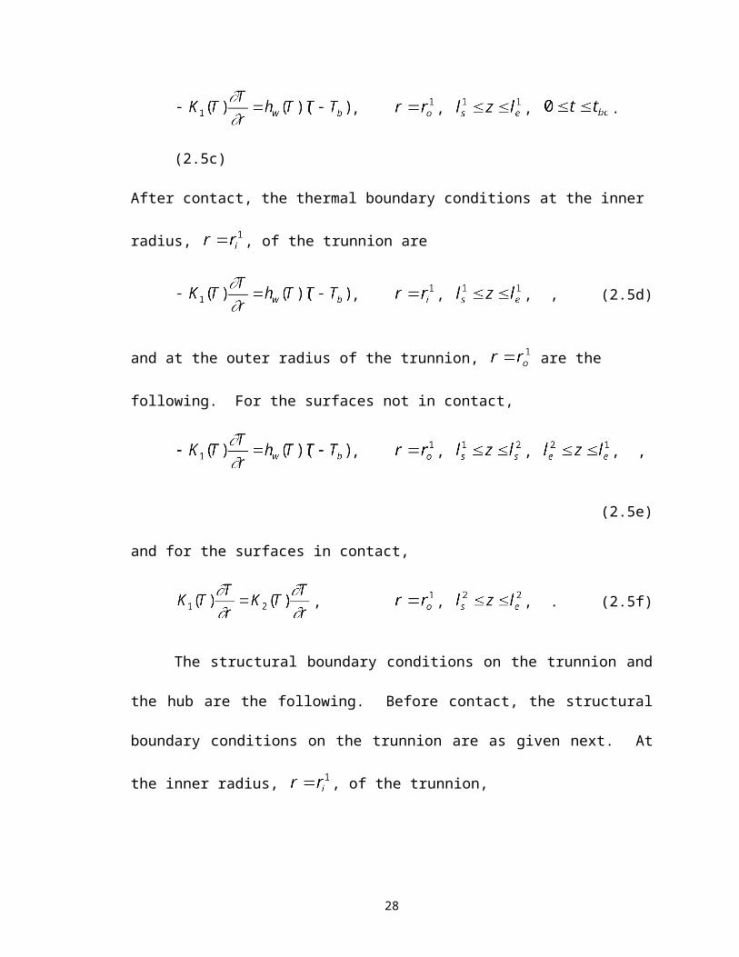
3.3.3 Complete analysis
Parameters obtained from previous thermal and structural analysis are used to
perform the complete thermal and structural analysis.
3.3.3.1 Process box-full thermal analysis
Parameters input for AP#1
thct1 - see Section 3.3.2.1
hgct1 - see Section 3.3.2.2
twarm1 - see Section 3.3.2.2
Parameters input for AP#2
hgct2 - see Section 3.3.2.1
thct2 - see Section 3.3.2.2
hwarm2 - see Section 3.3.2.1
Parameters output for AP#1
thwarm1 - the time at which the THG assembly meets the user defined exit
criterion when the trunnion-hub assembly is fitted into the girder (see
Section 4.3.5.2).
Parameters output for AP#2
twarm2 - the time at which the THG assembly meets the user defined exit
criterion when the trunnion is fitted into the hub-girder assembly (see
Section 4.3.5.2).
43
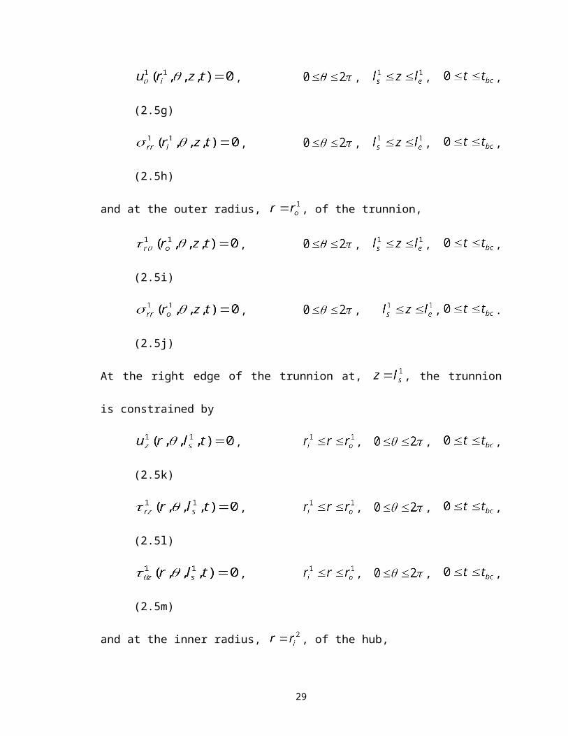
3.3.3.2 Process box-full structural analysis
The nodal temperatures from ‘full thermal analysis’ are transferred to this
analysis. The complete structural analysis is performed for both the assembly
procedures.
3.3.4 Ancillary analysis
The stand alone cooling down processes are performed.
3.3.4.1 Ancillary cooling 1
The following cooling process in performed: for AP#1 - cooling down of the
trunnion, and for AP#2 - cooling down of the hub.
3.3.4.2 Ancillary cooling 2
The following cooling process is performed: for AP#1 - cooling down of the
trunnion-hub, and for AP#2 - cooling down of the trunnion
Parameters input for AP#1
thct1 - time of contact between the trunnion and the hub (see Section 4.3.5.2).
This parameter is obtained from ‘structural analysis 1’.
twarm1 - time at which the trunnion-hub assembly fulfils user defined exit
criterion (see Section 4.3.5.2) during the insertion of the trunnion into
the hub.
Parameters input for AP#2
hgct2 - time of contact between the hub and the girder. This parameter is
obtained from ‘structural analysis 1’.
hwarm2 - time at which the hub-girder assembly fulfils user defined exit
criterion during the insertion of the hub into the girder.
44
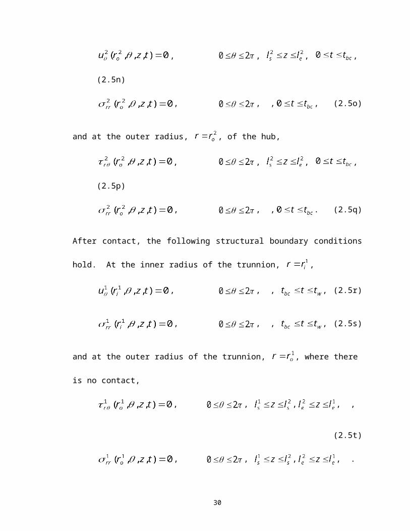
3.4 The finite element model
Table 3.1 describes the types of element used in the model with a brief description
of each.
The structural and thermal element meshes for the THG assembly are shown in
Figure 3.2a (brick elements) and Figure 3.2b (shell elements). Note that the sequential
coupled field analysis requires separate elements to be defined for both the thermal and
structural analysis. Hence, Figure3.2a and Figure 3.2b plot both the thermal and the
structural elements at the same time. The shell elements used to plot the gussets are
shown in Figure 3.2b. Figure 3.2c plots the contact and target elements and Figure 3.2d
plots the combination elements.
45
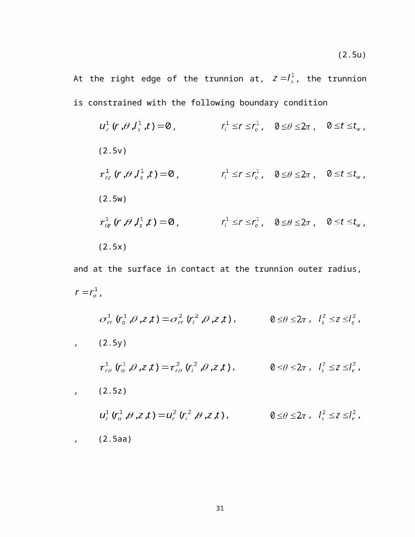
Table 3.1 Element characteristics.FIELD ELEMENT
NAMEDESCRIPTION
Thermal SOLID70 1. 3-D 8 node thermal brick element
2. Option to evaluate the convection coefficient as a function of wall temperature.
3. Thermal analogue of SOLID45
SHELL57 1. Three dimensional thermal shell element
2. Used to mesh the gussets
Structural SOLID45 1. 3-D 8 node structural element2. Structural analogue of
SOLID70SHELL63 1. Three dimensional structural
shell element2. Used to mesh the gusset
Contact CONTACT174 1. 3-D surface-to-surface structural contact.
2. Used to model structural contact between trunnion-hub and hub girder
TARGET170 1. Target element for CONTACT174.
2. Used to model structural contact between the hub and the girder
Combination COMBIN37 1. Used to create thermal contact between trunnion-hub and hub-girder
2. Allows thermal contact to be ‘switched on’ and ‘switched off’ based on the time parameter
46
Figure 3.2a Thermal element SOLID70 and structural element SOLID45.
Figure 3.2b Thermal element SHELL57 and structural element SHELL63.
47
Figure 3.2c Contact elements CONTACT174 and TARGET170.
Figure 3.2d COMBIN37 elements.
48
3.5 Assumptions
3.5.1 Sequential coupled field approach
The assumption in this approach is that the structural results are dependent upon
the thermal results but not vice-versa. This is a fair assumption as the effect of strains on
the thermal analysis is negligible.
3.5.2 Convection coefficient
The assumptions in the calculation of the convective heat transfer coefficient for air
are:
1. The geometry of the assemblies is assumed to cylindrical. To obtain the
convective heat transfer coefficient the Grashoff’s number ( ), Prandtl number (
) and the Nusselt number ( ) are required. The equations to obtain these
quantities are discussed next. Grashoff’s number is defined by Ozisik (1977) as
(3.1a)
where
g = acceleration due to gravity,
= volume coefficient of thermal expansion,
= wall temperature,
= ambient temperature,
= diameter of cylinder, and
= kinematic viscosity.
The Prandtl number, Pr is defined by Ozisik (1977) as
(3.1b)
where
49
cp = specific heat,
= absolute viscosity, and
k = coefficient of thermal conductivity.
The Nusselt’s number is defined by the following equation (Ozisik, 1977).
. (3.1c)
The convective heat transfer coefficient is also obtained from Ozisik (1977) as
. (3.1d)
2. The value for the hydraulic diameter, D, for the trunnion is the outer diameter of
the trunnion, for the hub, it is the hub outer diameter, and for the girder, it is the
length of the girder.
3. Turbulent flow is assumed.
4. The convection coefficient is assumed to be dependent on the wall temperature
and bulk or ambient temperature.
The convection coefficient for air is plotted later in this chapter. Note that the value for
the convective heat transfer coefficient is not a function of the hydraulic diameter.
Hence, the convective coefficient is independent of the bridge geometry.
3.5.3 Time increments and contact point
The minimum time increment in this model is one minute. Hence, the degree of
accuracy of our time of contact between parts of the assembly is less than one minute.
50
3.5.4 Finite element method assumptions
The standard inaccuracies associated with any finite element model due to mesh
density, time increments, number of substeps, etc. are present in this model (Logan,
1996).
3.5.5 Material properties
The material properties of the THG assembly, the air and the cooling medium are
temperature dependent and are evaluated at specified temperature increments. The
properties in between or outside the extremes of these values are interpolated and
extrapolated, respectively.
3.6 Nonlinear material properties of metal
The nonlinear material properties for a typical steel - Fe - 2.25 Ni (ASTM A203-A)
are plotted below. Though nonlinear material properties in general are explored,
particular emphasis is given to properties at low temperatures.
3.6.1 Young’s modulus
The elastic modulus of all metals increases monotonically with increase in
temperature. The elastic modulus can be fitted into a semi-empirical relationship:
(3.2)
where
= elastic constant at absolute zero,
= constant, and
= Einstein characteristic temperature.
The Young’s modulus remains stable with change in temperature (see Figure 3.3)
and hence is assumed to remain constant throughout this analysis.
51
Figure 3.3. Young’s modulus of steel as a function of temperature.
3.6.2 Coefficient of thermal expansion
The coefficient of thermal expansion at different temperatures is determined
principally by thermodynamic relationships with refinements accounting for lattice
vibration and electronic factors. The electronic component of coefficient of thermal
expansion becomes significant at low temperatures in cubic transition metals like iron
(Reed, 1983). The coefficient of thermal expansion increases with increase in
temperature by a factor of three from –3210F to 800F as shown in the Figure 3.4.
52
Figure 3.4 Coefficient of thermal expansion of steel as a function of temperature.
3.6.3 Thermal conductivity
The coefficient of thermal conductivity (see Figure 3.5) increases with an increase
in temperature by a factor of two from –3210F to 800F. Thermal conduction takes place
via electrons, which is limited by lattice imperfections and phonons. In alloys, the defect
scattering effect ( is more significant than the phonon scattering effect ( (Reed,
1983).
53
Figure 3.5 Thermal conductivity of steel as a function of temperature.
3.6.4 Density
For the range of temperatures of interest to our study the density remains nearly
constant, as shown in Figure 3.6.
Figure 3.6 Density of steel as a function of temperature.
54
3.6.5 Specific heat
Lattice vibrations and electronic effects affect the specific heat of a material. The
contribution of two effects can be shown by
(3.3)
where,
= lattice contribution,
= volume coefficient of thermal expansion,
= electronic contribution, and
= normal electronic specific heat.
Note that specific heat decreases by a factor of 5 over the temperature range in question,
as shown in Figure 3.7.
Figure 3.7 Specific heat of steel as a function of temperature.
3.7 Nonlinear material properties of air and liquid nitrogen
55
The temperature dependent convective heat transfer coefficients for air and liquid
nitrogen are plotted next.
3.7.1 Convection to air at 800F
The convective heat transfer coefficient is a function of the volume coefficient of
thermal expansion ( ), the thermal conductivity ( ), absolute viscosity ( ), kinematic
viscosity ( ), specific heat ( ) and mass density ( ) all of which are temperature
dependent. The Grashof number, the Nusselt number and the Prandtl number and
ultimately the convective heat transfer coefficient can be calculated from these quantities
from Equations (3.1a) through (3.1d). The variation of each with temperature is plotted
in Figure 3.8a through Figure 3.8f.
Figure 3.8a Volume coefficient of thermal expansion of air as a function of temperature.
56
Figure 3.8b Thermal conductivity of air as a function of temperature.
Figure 3.8c Kinematic viscosity of air as a function of temperature.
57
Figure 3.8d Specific heat of air as a function of temperature.
Figure 3.8e Absolute viscosity of air as a function of temperature.
58
Figure 3.8f Mass density of air as a function of temperature.
The convective heat transfer coefficient for air, based upon the previous five graphs and
Equations (3.1), is shown in Figure 3.8g. Note that the convective heat transfer
coefficient for convection to air is evaluated at the film temperature (that is, the average
of the bulk and wall temperatures).
Figure 3.8g Convective heat transfer coefficient of air as a function of temperature.
59
3.7.2 Convection to liquid nitrogen at –3210F
The phenomenon of convection to liquid nitrogen is quite complex and involves
multi-phase heat transfer. Whenever an object at ambient temperature (that is, 80F)
comes into contact with liquid nitrogen “film boiling” occurs until the temperature of the
object reaches approximately –260F. This phenomenon of film boiling occurs when
there is a large temperature difference between the cooling surface and the boiling fliud.
At the point when film boiling stops, the minimum heat flux occurs and the phenomenon
of “transition boiling” occurs until the temperature of the object reaches –290F. At the
point when transition boiling stops, the maximum heat flux occurs and the phenomenon
of “nucleate boiling” occurs until the temperature of the object reaches the temperature of
liquid nitrogen. Nucleate boiling occurs when small bubbles are formed at various
nucleation sites on the cooling surface. When nucleate boiling starts the object cools
very rapidly.
The convective heat transfer coefficient for convection to liquid nitrogen is
dependent on many factors, such as, surface finish, size of the object and shape of the
object, to name a few. Based on the previous discussion, the convective heat transfer
coefficient for convection to liquid nitrogen is shown in Figure 3.9 (Brentari and Smith
1964). This data was chosen because it very closely matches the surface finish, and
object sizes and shapes used for trunnions and hubs. Note that the convective heat
transfer coefficient for convection to liquid nitrogen is evaluated at the wall temperature.
60
Figure 3.9 Convective heat transfer coefficient of liquid nitrogen as a function of temperature.
61
17.37
0.069
CHAPTER 4
USER MANUAL
4.1 Introduction
One of the principal contributions of this work is creating a user friendly
parametric model, which shall henceforth be called the Trunnion-Hub-Girder Testing
Model (THGTM), to analyze existing Trunnion-Hub-Girder (THG) assemblies and
design new assemblies. A step-by-step guide for using the THGTM is presented in this
chapter. The program allows the user to analyze existing assemblies and design new
assemblies. The two assembly procedures, assembly procedure 1 (AP#1) and assembly
procedure 2 (AP#2), are modeled in the THGTM. This program allows the user to
change materials, meshing parameters, loads and time increments. One useful feature of
this program is that it allows the user to determine the exit points during the different
steps in the analysis (see Section 4.3.5.2). Results are presented both in time history
graphs (position fixed) and contour plots (time fixed).
The THGTM has a user-friendly interface in the form of dialog boxes, pick menus
and toolbars. While every attempt has been made to make the program simple and user
friendly, this has not been achieved at the cost of denying the user the flexibility over
issues such as mesh density, computational time and accuracy. It is assumed that the user
has some basic knowledge of finite elements with regards to element shape testing,
thermo-structural field interaction, effects of mesh refinement on computational time, and
cost (computational time) - accuracy trade-off. The user should read Chapter 3 to
62
understand and appreciate the modeling approach and assumptions used in the model.
The program has been written principally in ANSYS Parametric Design Language
(APDL) including a few commands from User Interface Design Language (UIDL).
4.2 Modeling of the assembly procedures
During the actual assembly of the trunnion-hub-girder (THG), the male part is
cooled down till there is a clearance between the two parts of the assembly. Initially,
convection with air and conduction in the gap between the two parts results in the parts
coming into contact. After contact, conduction at the contact surfaces and convection
with air at the free surfaces results in an interference fit between the two parts of the
assembly. However, due to difficulties in modeling dynamic gap conduction using the
sequential coupled field approach, a modified approach is used. In this model, the male
part of the assembly is inserted in the female part as soon as the interference between the
two parts is breached and hence no gap conduction is modeled.
The two cooling processes in each assembly procedure are analyzed separately
and the results presented in ancillary files.
4.3 Running the trunnion-hub-girder testing model
A step-by-step guide to run the THGTM is presented next.
4.3.1 Starting the trunnion-hub-girder testing model
4.3.1.1 Step 1
On the desktop go the START menu and enter
START>Programs>ANSYS 5.5> Interactive
The interactive window in Figure 4.1 is displayed.
63
Figure 4.1 Interactive.
Working directory: This directory contains all the ANSYS files. If one of the drives is
approaching capacity the working directory can be changed. The following files,
available at www.eng.usf.edu/~besterfi/bascule must be copied to the new working
directory.
thgtm1.mac: Input file for AP#1
thgtm2.mac: Input file for AP#2
hills: parameters for the Hillsborough Avenue Bridge
hallen1: parameters for the Hallendale Beach Boulevard Bridge
christa: parameters for the Christa McAuliffe Bridge
cause17: parameters for the 17th Street Causeway Bridge
thpost.mac: input file for the time-history postprocessor
64
Working directory where the ANSYS files
are stored
Choose Win32
Default Jobname can be changed
later
Recommended 600
Recommended 200
Yes
Only US English allowed
Press run
myset.mac: input file for dimensioning the parameters
There is also a file ndraw.mac in the c:\tdraw directory. Do not delete any of these files.
If you do delete them inadvertently then go to www.eng.usf.edu/~besterfi/bascule and
download the files again. If you want to move this program to another computer, then do
the following three steps.
1. Copy ‘Start55.ans’ from D:\ANSYS55\DOCU to the new \ANSYS55\DOCU
directory of the drive where ANSYS is installed.
2. Copy all the required files to the new working directory.
3. Create a new directory c:\tdraw and copy ndraw.mac into it.
4.3.1.2 Step 2
On clicking on RUN in ANSYS 5.5, interactive menu shown in Figure 4.3.1.1 the
various ANSYS windows and input menus appear on the screen as shown in Fig 4.3.1.2.
A description of the menus and windows:
Main Menu: The main menu is the interactive interface for the ANSYS processors,
operations and preferences.
Utility Menu: The utility menu is for performing the file operations and other non-
processor dependent operations in ANSYS.
Output Window: The ANSYS output window displays the output of the ANSYS
operations. In this model the output is not shown on the output window. Instead it is
directed to an output file.
ANSYS Toolbar: The toolbar has many tools which will be used in the THGTM.
Graphics Window: The graphical output (solid model, meshing, results etc.) are displayed
in the ANSYS graphics window
65
Figure 4.2 ANSYS windows.
4.3.1.3 Step 3
Go to the ANSYS toolbar as shown in Figure 4.3 and click on THG1 for AP#1
and THG2 for AP#2.
Figure 4.3 ANSYS toolbar (assembly procedure).
66
Utility menuToolbar
Input menu
Main menuOutput window
AP#1
AP#2
4.3.2 Entering filenames
The filenames of the different parts of the analysis are entered in this section. As
we are using a sequential coupled field process, both structural and thermal filenames are
required for any run. Step 4 and Step 5 allow the user to enter the filenames for the
complete thermal and structural analyses while Step 6, Step 7, Step 8, Step 9 allow the
user to enter filenames for the ancillary analyses. Note that all filenames must be entered
in single quotes. For example for the Hillsborough Bridge using AP#1 the thermal
filename can be ‘Thill1’.
4.3.2.1 Step 4
The thermal filename for the complete analysis is entered in the dialog box shown
in Figure 4.4.
Figure 4.4 Thermal filename.
4.3.2.2 Step 5
The structural filename for the complete analysis is entered in the dialog box
shown in Figure 4.5
67
Default filename
Figure 4.5 Structural filename.
4.3.2.3 Step 6
For AP#1, the thermal filename for the cooling down of the trunnion is entered in
the dialog box shown in Figure 4.6a
Figure 4.6a Trunnion cooling thermal filename.
For AP#2, the thermal filename for the cooling down of the hub is entered in the dialog
box shown in Figure 4.6b.
Figure 4.6b Hub cooling thermal filename.
4.3.2.4 Step 7
For AP#1, the structural filename for the cooling down of the trunnion is entered
in the dialog box shown in Figure 4.7a.
68
Default filename
Default filename
Default filename
Figure 4.7a Trunnion cooling structural filename.
For AP#2, the structural filename for the cooling down of the hub is entered in the dialog
box shown in Figure 4.7b.
Figure 4.7b Hub cooling structural filename.
4.3.2.5 Step 8
For AP#1, the thermal filename for the cooling down of the trunnion-hub is
entered in the dialog box in Figure 4.8a.
Figure 4.8a Trunnion-hub cooling thermal filename.
For AP#2, the thermal filename for the cooling down of the trunnion is entered in the
dialog box shown in Figure 4.8b.
69
Default filename
Default filename
Default filename
Figure 4.8b Trunnion cooling thermal filename.
4.3.2.6 Step 9
For AP#1, the structural filename for the cooling down of the trunnion-hub is
entered in the dialog box shown in Figure 4.9a.
Figure 4.9a Trunnion-hub cooling structural filename.
For AP#2, the structural filename for the cooling down of the trunnion is entered in the
dialog box shown in Figure 4.9b.
Figure 4.9b Trunnion cooling structural filename.
A series of error messages shown in Figure 4.9c will appear.
70
Default filename
Default filename
Default filename
Figure 4.9c Error message.
These error messages are caused due to a bug in the ANSYS software and do not affect
the program in any way. Keep on clicking OK to ignore the errors till the next multi-
prompt dialog box appears.
4.3.3 Material and geometric parameters
The steps described in this section allow the user to enter material and geometric
parameters. The user is given the choice of using one of the existing geometries of the
THG assemblies or entering his/her own geometrical parameters.
4.3.3.1 Step 10
A multi-prompt dialog box similar to the one shown in Figure 4.10 appears
allowing the user to choose the material of the THG assembly.
Figure 4.10 Material choice menu.
71
4.3.3.1 Step 11
The user is given a choice between using the existing geometries for the bridges
or entering his or her own geometric parameters. The multi-prompt dialog box shown in
Figure 4.11 allows the user to choose between the following: choice=1 is to use one of
the saved bridges and choice=2 is to design a new bridge.
Figure 4.11 Bridge options.
The next step depends upon the ‘choice’ parameter entered in Step 11. Ignore all the
error messages till you get the next multi-prompt dialog box.
4.3.3.3 Step 12 (choice=1)
This option allows you to choose one of the existing THG assemblies. Ignore all
the error messages till you get multi-prompt dialog box similar to the one shown in
Figure 4.12.
72
Figure 4.12 Bridge choices.
The multi-prompt dialog box shown in Figure 4.12 allows the user to choose between the
following: bridge=1 is to use Hillsborough Avenue Bridge, bridge=2 is to use Hallendale
Beach Boulevard Bridge, bridge=3 is to use Christa McAuliffe Bridge, and bridge=4 is to
use 17th Street Causeway Bridge.
4.3.3.4 Step 12 (choice=2)
This option allows you to build a THG assembly with user defined geometric
parameters. Ignore all the error messages till you get a multi-prompt dialog box. The
default parameters are set for the Christa McAuliffe Bridge.
4.3.3.4.1 Step 12a (choice=2)
Figure 4.13a shows the trunnion dimensions to be entered. All dimensions are in inches.
73

Figure 4.13a Trunnion dimensions.
The dimensional parameters to be entered are
lt = total length of the trunnion,
l = Extension of the trunnion on the gusset side (length to hub on the
trunnion on the gusset side),
lh = total length of the hub,
rti = inner radius of the trunnion, and
rto = outer radius of the trunnion (inner radius of the hub)
Figure 4.13b shows the multi-prompt dialog box for entering the trunnion dimensions.
74
lt
lhlcontact
region with hub on
outside of trunnion
rto
rti
Figure 4.13b Trunnion dimension parameters.
After entering the trunnion parameters click OK. Ignore the error messages by
clicking OK to each of them till the next multi-prompt dialog box appears on the screen.
4.3.3.4.2 Step 12b (choice=2)
The hub dimensions to be entered are shown in Figure 4.3.3.4.2a. All dimensions
are in inches.
75
Figure 4.14a Hub dimensions.
The dimensional parameters to be entered are
rhg = outer radius of the hub (minus flange),
rho = outer radius of the hub flange,
wbr = backing ring width,
wgw = width of the girder (web),
whf = width of hub flange,
lf = distance to hub flange,
lh = total length of the hub,
tg = gusset thickness, and
ex = distance from the end of the backing ring to the end of the hub.
76
rhg
rho
lf whf
wgw
wbrr
ex
lh
Hub-girder contact area
Hub-backing ringcontact area
The hub dimensions can be entered in the multi-prompt dialog box shown in Figure
4.14b.
Figure 4.14b Hub dimension parameters.
After entering the trunnion parameters click OK. Ignore the error messages by
clicking OK to each of them till the next multi-prompt dialog box appears on the screen.
77

4.3.3.4.3 Step 12c (choice=2)
The dimensions to be entered for the girder are shown in Figure 4.15a.
All dimensions are in inches.
Figure 4.15a Girder dimensions.
The dimensional parameters to be entered are
wgf = width of the girder flange,
hgw = height of the girder web,
lg = width of the girder,
hgf = height of the girder flange, and
wgw = width of the girder web.
The girder dimensions can be entered in the multi-prompt dialog box shown in Figure
4.15b.
78
wgw
hgwrhg
hgf
lg
wgf
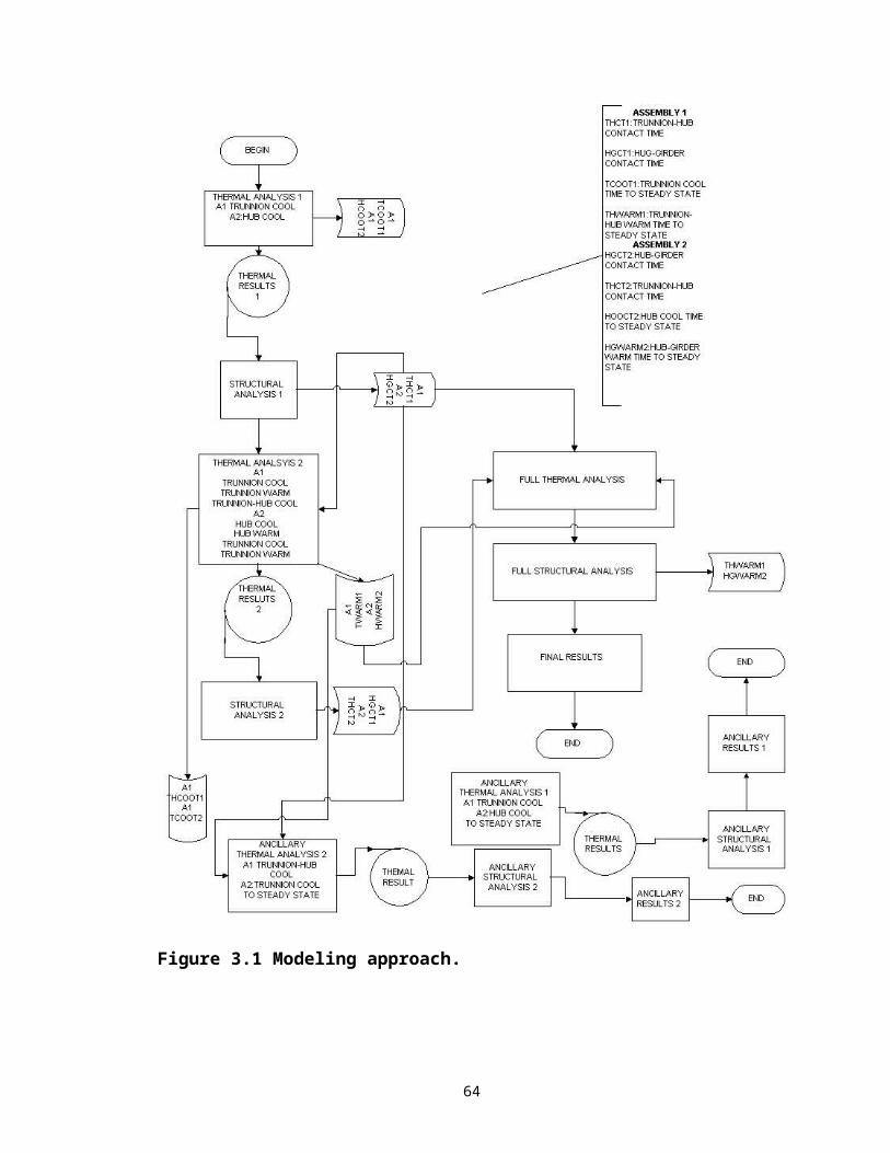
Figure 4.15b Girder dimension parameters.
Click OK to ignore all the error messages till the next multi-prompt dialog box appears
on the screen.
4.3.4 Meshing input
The meshing details of the THG assembly are entered here. Some meshing
parameters have restrictions as regards to the range of values that can be used. The
acceptable values are shown in the parentheses for these parameters.
4.3.4.1 Step 13
The divisions along the girder are entered here. Figure 4.16a shows the girder
division parameters to be entered.
79
Figure 4.16a Girder divisions.
The girder division parameters to be entered are
gfdiv = number of divisions along the girder flange width, and
hgfdiv = number of divisions along the girder flange height
Figure 4.16b shows the multi-prompt dialog box where the girder dimension parameters
to be entered.
Figure 4.16b Girder division parameters.
80
hgfdivgfdiv
After entering the parameters click OK. Ignore all the error messages till the next multi-
prompt dialog box appears on the screen.
4.3.4.2 Step 14
Meshing parameters along the length, that is, number of divisions along the length
are during this step. Figures 4.17a and 4.17b show the meshing parameters to be entered.
Figure 4.17a Divisions along the length (trunnion).
The meshing parameters to be entered are
fdiv = number of divisions along the length to the hub on the gusset side, and
ldiv = number of divisions along the length to the hub on the backing ring
side.
81
fdiv ldiv
contact region with
hub on outside of trunnion
Figure 4.17b Divisions along the length (hub).
The relevant dimensional parameters are explained in Sections 4.3.3.4.1, 4.3.3.4.2
and 4.3.3.4.3.
fdiv = number of divisions along f,
exdiv = number of divisions along ex,
whfdiv = number of divisions along whf,
wbrdiv = number of divisions along wbr,
wgwdiv = number of divisions along wgw,
whfdiv = number of divisions along whf,
82
Hub-girder contact area
Hub-backing ringcontact area
lfdiv
whfdiv
wgwdiv
wbrdiv
exdiv
lfdiv = number of divisions along lf, and
ldiv = number of divisions along l.
Figure 4.17c shows the multi-prompt dialog box where the parameters are to entered.
Figure 4.17c Divisions along the length parameters.
After entering the parameters click OK. Ignore the error messages till the next multi-
prompt dialog box appears on the screen.
4.3.4.3 Step 15
Some more meshing parameters, such as, number of radial and circumferential
divisions, are entered here. The number of radial divisions is the same for the trunnion,
83
hub and the girder. This is done so that the components contact each other smoothly.
Figures 18a, 4.18b and 4.18c show the radial and circumferential divisions to be entered
for the trunnion, the hub and the girder
Figure 4.18a Trunnion radial and circumferential divisions.
Figure 4.18b Hub radial and circumferential divisions.
84
numdiv
cdiv
numdivnumdiv
cdiv
Figure 4.18c Girder radial and circumferential divisions.
The radial and circumferential divisions to be entered are:
numdiv = number of divisions in the radial direction in each the trunnion, the
hub and the girder, and
cdiv = number of divisions in the circumferential direction for every 600
(between a pair of gussets).
Note that restricted values for ‘numdiv’ are odd numbers greater or equal to three (that is,
3, 5, 7, 9, …), and restricted numbers for ‘cdiv’ are multiples of 4 (that is, 4, 8, 12, …).
Figure 4.3.4.3d shows the multi-prompt dialog where the radial and circumferential
parameters are to be entered.
85
numdiv
cdiv
numdiv
Figure 4.18d Radial and circumferential division parameters.
Click OK. Ignore all the error messages which follow till the next multi-prompt dialog
box appears on the screen.
4.3.4.4 Step 16
The radial interference between the trunnion and hub (thInt) and the hub and
girder (hgInt) are entered at this step. The interference values for FN2 and FN3 fits can
be obtained using the Bascule Bridge Design Tools (Denninger, 2000). Click OK after
entering the values. All parameters to be entered are in inches. Ignore the error messages
till you get the next multi-prompt dialog box (see Figure 4.19) and the hourglass cursor
changes back into the arrow.
86
Figure 4.19 Radial interference.
4.3.5 Loading input
4.3.5.1 Step 17
The cooling medium bulk temperature (Tcool) and the ambient air bulk
temperature (Tbulk) are to be entered in the multi-prompt dialog box shown in Figure
4.20. Note that all units are 0F. After entering the values, click OK. Ignore the series of
error messages by clicking OK till you get a multi-prompt dialog box.
Figure 4.20 Applied thermal loads.
87

4.3.5.2 Step 18
The time temperature and time increment options are entered in this step.
AP#1 and AP#2 have different input files and hence have their own distinct set of input
parameters.
For AP#1, the time-temperature options are entered in the multi-prompt dialog
box shown in Figure 4.21a. An explanation of the parameters to be entered is also
included in this section.
Figure 4.21a Time-temperature options (AP#1).
88
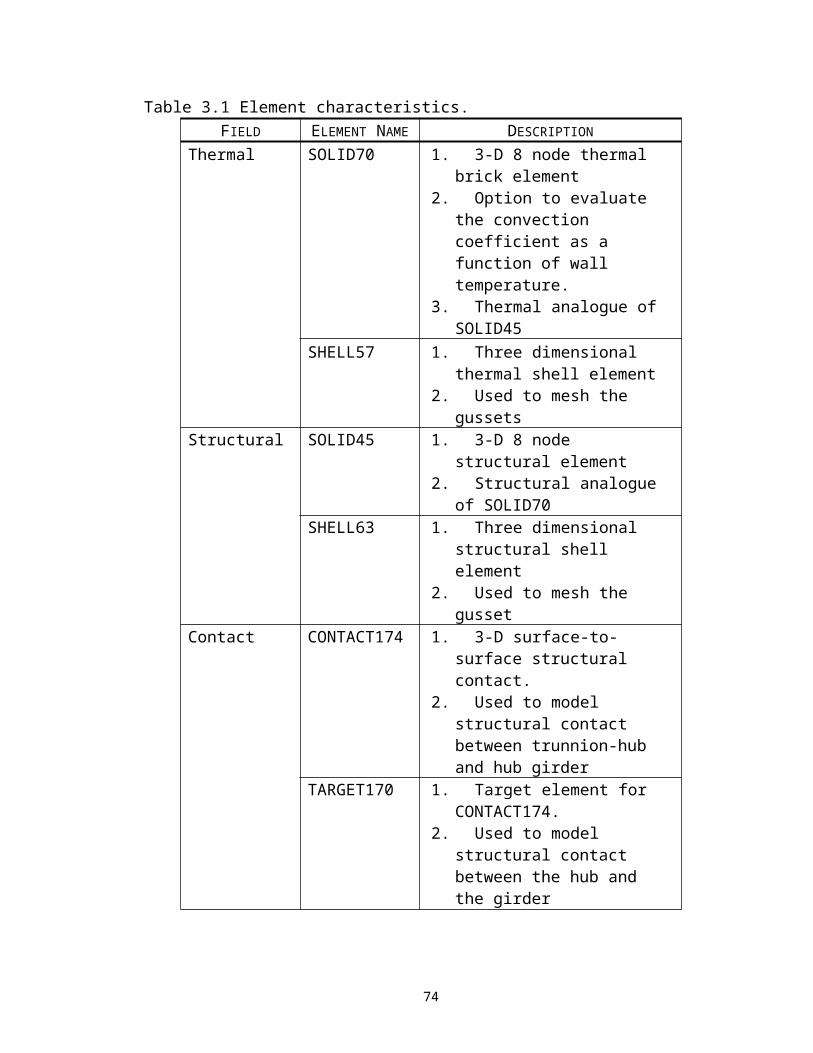
For AP#2, the time-temperature options are entered in the multi-prompt dialog
box shown in Figure 4.21b.
Figure 4.21b Time –temperature options (AP#2).
Reference strain temperature (myref): The reference temperature is the temperature at
which the strains are zero. Normally, the reference temperature should be the same as
the ambient air temperature. The ambient air temperature should be entered unless
the reference temperature is different from ambient air temperature.
Time increments for warming (tinc, tinc2) and time increments for cooling (tincc, tincc2):
The time increments denote the time intervals at which the results are saved. The
larger the time increment, the less accurate the result, the fewer the points on the load
89
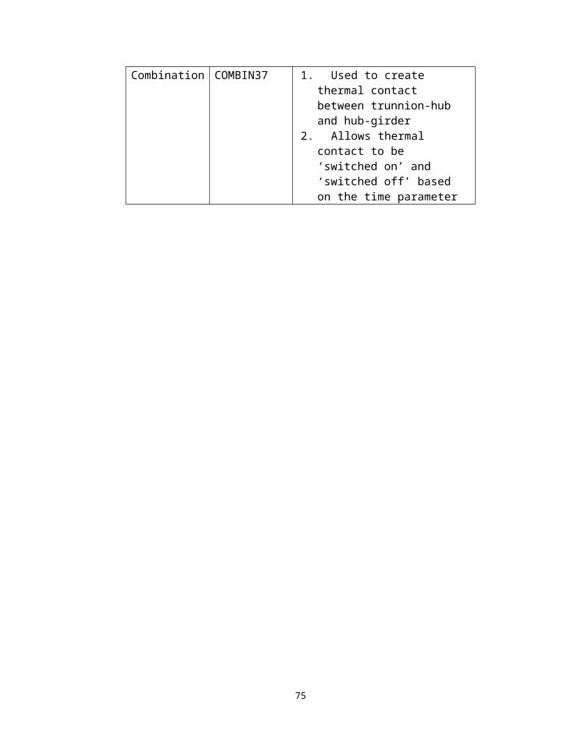
history and hence the less is the computational time. Time increments for the
warming and cooling process should be chosen balancing the needs of accuracy,
conserving computational time and required number of points in the loading history.
Typically, the time increments during warming could be a larger (25-200 minutes)
than the time increments during cooling (1-4 minutes) as warming is a slower process
than cooling. The values in the brackets are only a suggested range of values. The
user can choose any integer time increment he or she deems fit.
Cool temperature factor (cptemp): This parameter determines the point at which the
cooling process is to be stopped. The cooling process stopped once the minimum
temperature in the assembly falls below the stop temperature determined by Equation
(4.1a)
(4.1a)
where
= warm temperature criterion,
= ambient air bulk temperature, and
= cooling medium bulk temperature.
Note that, large values (0.95 to 0.9999) are recommended for the cool temperature
factor. In this model we use the sequential coupled field approach and hence, the
thermal analysis for the cooling process is performed before the structural analysis.
‘cptemp’ determines the parameter for exiting the thermal analysis during cooling. If
a small value of cptemp is used then it can cause the thermal analysis to exit even
before the time point at which the gap between the two bodies is breached in the
structural analysis. However, the cptemp=1 should not be used as a body
90

theoretically attains the bulk temperature of the surrounding medium only after
infinite units of time.
Warm temperature factor (hptemp1 and hptemp2): The duration of the warming up
process is determined by the warm temperature factor. The warming up process is
stopped once the minimum temperature in the assembly exceeds the temperature
determined by the stop temperature determined by Equation (4.1b).
=1, 2 (4.1b)
where,
= cool temperature criterion,
= ambient air bulk temperature,
= cooling medium bulk temperature, and
= warm temperature factor for each of the two warming up
processes.
In Equation (4.1b), i=1, 2 denotes the first warming up process and the second
warming up process, respectively.
4.3.5.3 Step 19
Additional parameters required for performing the stand alone runs of the cooling
processes are entered in this step, that is, the time for which each cooling process is to be
analyzed. For AP#1 the ancillary cooling parameters are entered in Figure 4.22a. where
coolt1 is the trunnion cooling time and coolt2 is the trunnion-hub cooling time.
91
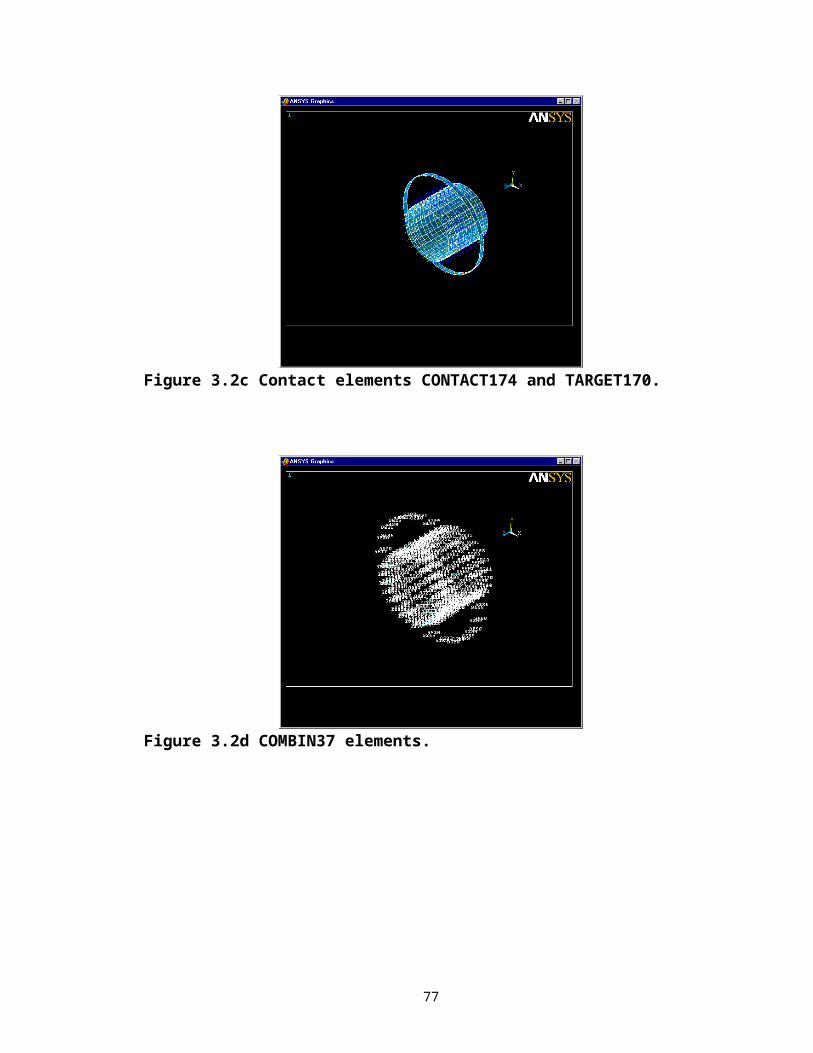
Figure 4.22a Ancillary cooling parameters (AP#1).
For AP#2, the ancillary cooling parameters are given in Figure 4.22b where coolt1 is the
hub cooling time and coolt2 is the trunnion cooling time.
Figure 4.22b Ancillary cooling parameters (AP#2).
92
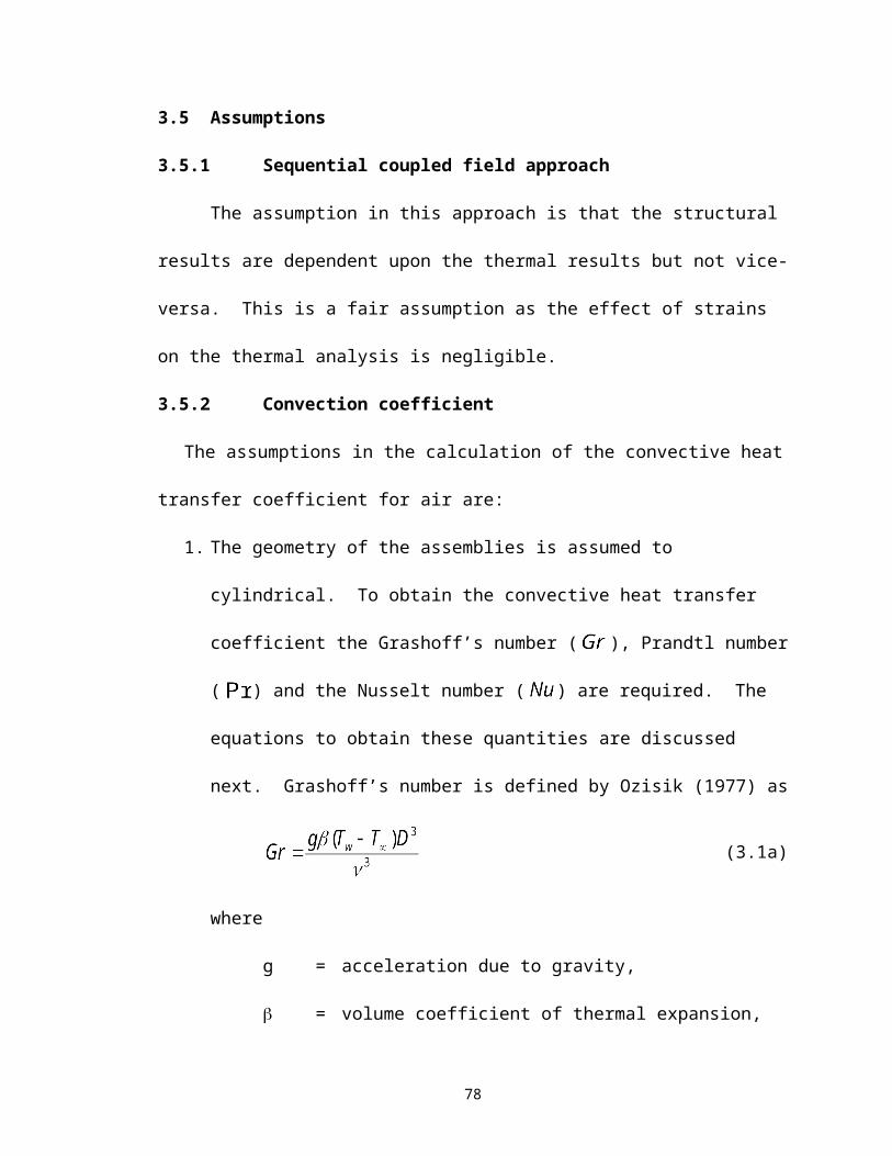
4.3.5.4 Step 20
In this step we define the equation of fracture toughness as a function of
temperature. Figure 4.23a shows the multi-prompt dialog box where the coefficients and
the constants are entered. The factor for the edge effects is also input in this step. The
equation of fracture toughness is assumed to be a fourth degree equation of temperature
, (4.2a)
where fourth, third, second, first, T and cterm are coefficient coefficients of the equation.
The critical crack length, , is given by
(4.2b)
where
= temperature dependent critical stress intensity factor,
= edge effects factor, and
= hoop stress.
93
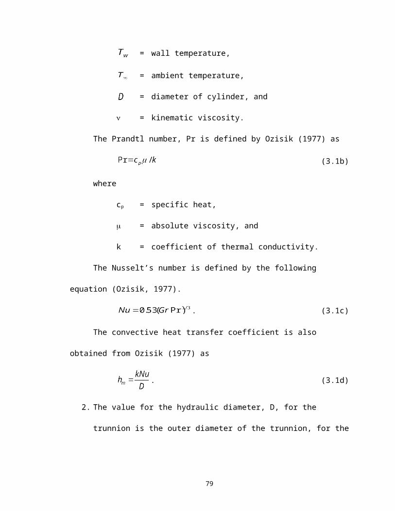
Figure 4.23a Fracture coefficients and constants.
After entering all of the parameters required for the run in Figured 4.23a, click OK. The
time required for the solution to run depends upon mesh density, time increments,
temperature factors, time parameters, meshing prameters, temperature factors and
ancillary parameters. While the solution is running, Figure 4.23b appears on the screen.
Figure 4.23b ANSYS process status bar.
94
The time required to complete a run depends on the bridge, meshing parameters,
time increments, temperature factors and ancillary parameters. A run takes a minimum
of 5 hrs. Once the ANSYS process status bar shown in Figure 4.23b disappears from the
screen, the solution is complete and ready for further post-processing. The required
ANSYS files have been saved in the working directory. Go to Sections 4.5 and 4.6 to do
the post-processing. Note that, the program does not have exit options or warnings if
wrong values are entered. Hence, if any wrong values are input, exit ANSYS by pressing
Ctrl+Alt+Del.
Once the solution is complete, pick all the ANSYS processes shown in Figure
4.23c and end them by clicking on END TASK.
95
Figure 4.23c Task manager.
4.3.6 Trunnion-hub-girder testing model crash
The THGTM can crash due to two possible situations. In Situation 1 the
disk drive is full and there is no space to store the ANSYS files. The remedy for this
situation is to free up some disk space and run the program again. In Situation 2 ANSYS
is out of memory. This situation is unlikely as the recommended values should normally
96
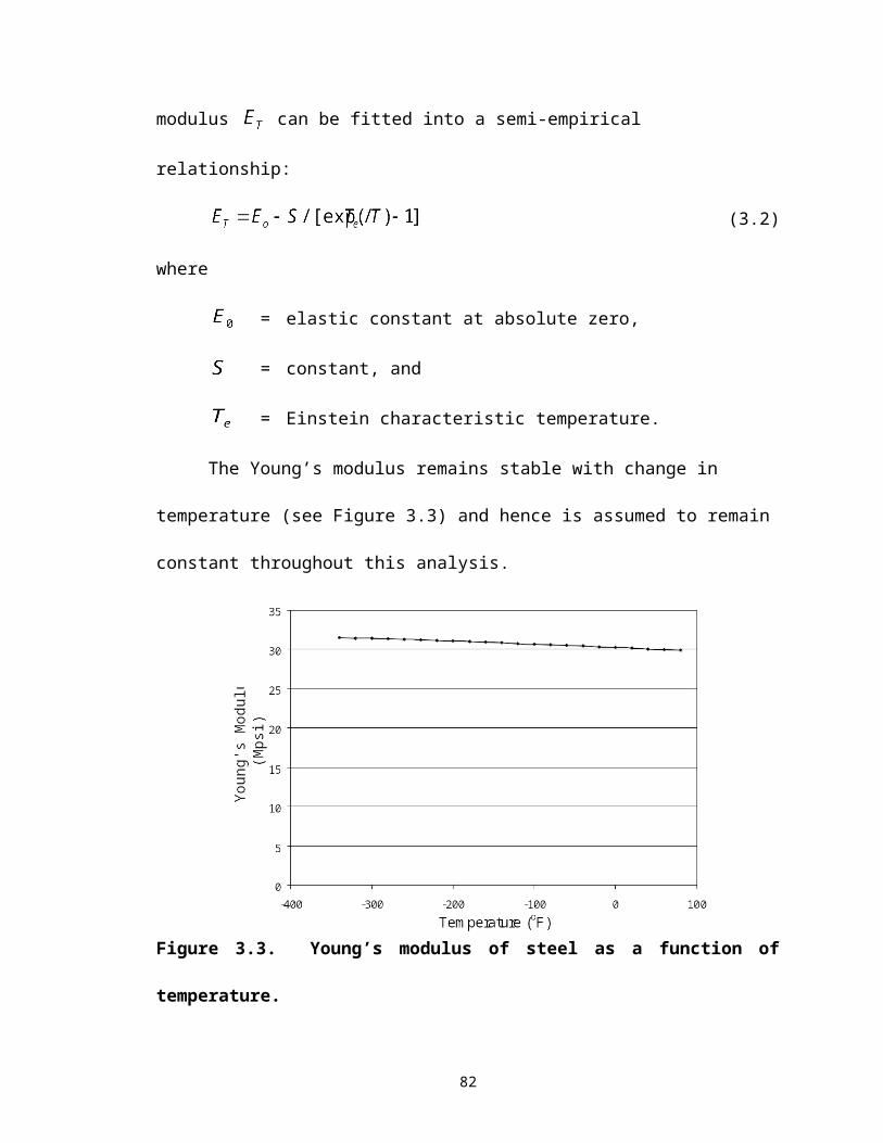
be sufficient. The remedy for this situation is to increase the database space and
workspace memory in interactive menu in Step 1 (refer to Figure 4.1) of Section 4.3
4.4 Resuming an already saved job
This section describes how the results of previous runs can be reviewed.
4.4.1 Step 1
Follow Step 1 and Step 2 of Section 4.3, that is, enter
File>Utlilty menu>Change jobname
The textbox in the Figure 4.24 asks the user to ‘enter a new jobname’. The user should
enter the jobname of the previously saved runs. Note that, filenames in the THGTM are
case sensitive.
Figure 4.24 Enter filename.
The filename must correspond to one of the previously saved runs. The filename
to be entered will depend upon the type of post-processing to be performed subsequently.
To enter one of the two post-processors, follow the guidelines presented next.
General Postprocessor:
Stresses: Enter the name of the structural file in Figure 4.24.
Temperatures: Enter the name of the thermal file in Figure 4.24.
Time history postprocessor:
Stresses and temperatures: Enter the name of structural file in Figure 4.24.
Once the filename is entered, click OK.
97
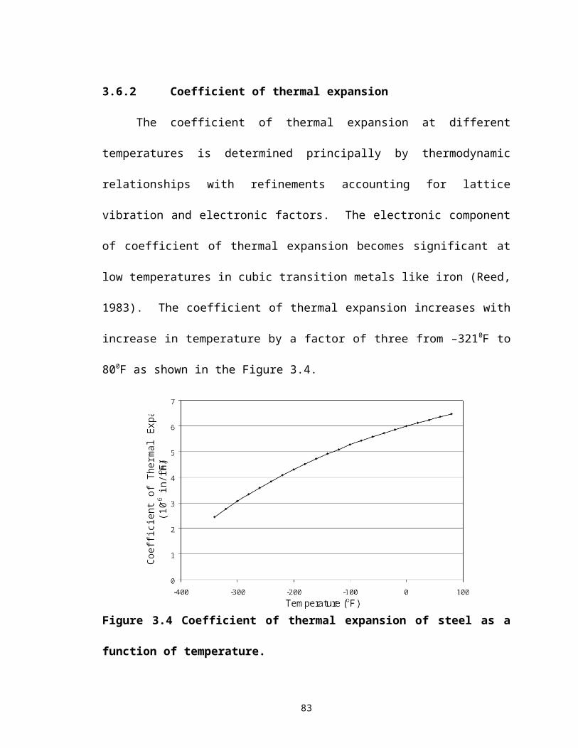
4.4.2 Step 2
Go to the Utility menu and enter the following.
File>Utility Menu>Resume Jobname.db
4.4.3 Step 3
On the ANSYS toolbar (see Figure 4.25a) click on DIMSET
Figure 4.25a ANSYS toolbar (set dimensions).
This step is required to dimension some arrays and set the results to the last set. The
results can now be seen in the general postprocessor (described in Section 4.5) or in the
time history postprocessor (described in Section 4.6). Sometimes on clicking DIMSET
you will get a series of messages similar to the one shown in Figure 4.25b.
Figure 4.25b Re-dimensioning verification box.
Keep clicking ‘yes’ till such messages don’t appear anymore. Note that if you fail to
click the DIMSET button on the ANSYS toolbar, the general postprocessor and the time
history postprocessor may not work as desired.
4.5 General postprocessor
The General postprocessor allows us view the results in the form of contour plots
(time fixed). Prior to performing the steps described next the user should have either:
98
Click here
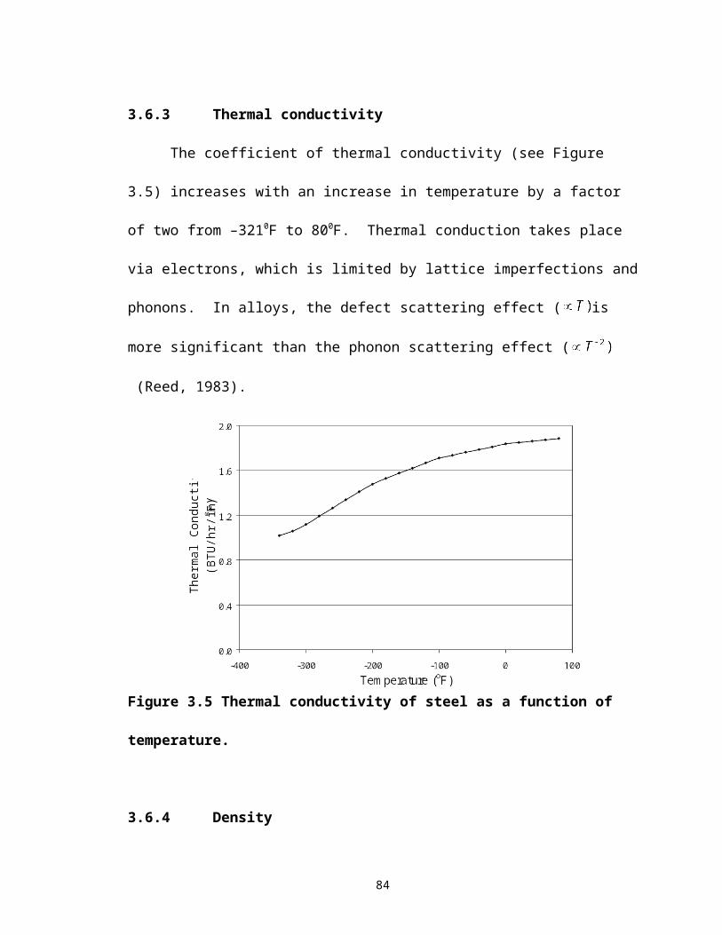
1. Performed a run of the program (Step 1 to Step 20) in Section 4.3, or
2. Resumed a previous run (Step 1 to Step 3) of Section 4.4.
4.5.1 Step 1
Choose the time point of interest by entering the following.
ANSYS Main Menu>General Postproc>Results Summary
Figure 4.26 shows a summary of the results. The first column ‘SET’ denotes the
set number of the results, ‘TIME/FREQ’ denotes the time for which the results have been
saved, ‘LOAD STEP’ denotes the load step number of the results, and ‘SUBSTEP’
denotes the number of substeps in a loadstep. In the results summary make a note of the
point of interest.
Figure 4.26 Results summary.
4.5.2 Step 2
Go to the ANSYS Main Menu and enter the following.
ANSYS Main Menu> General Postproc>-Read Results-By Time-Frequency
Enter the time of interest chosen from the results summary described in Section 4.5.2 in
the dialog box shown in Figure 4.27.
99
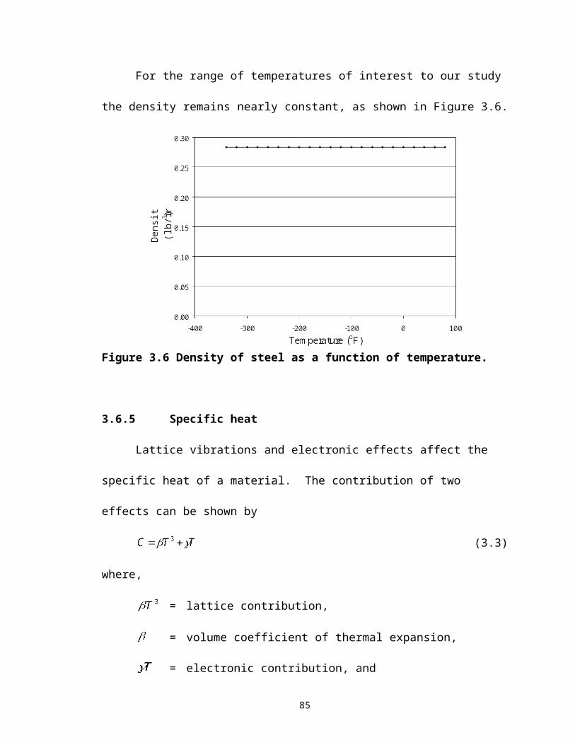
Figure 4.27 Read results.
4.5.3 Step 3
Go to the ANSYS Main Menu and enter the following.
ANSYS Main Menu> General Postproc>Plot Results> Nodal Solu
The dialog box shown in Figure 4.28a appears. Pick the quantity that needs to be plotted
and click OK. Note that, the results are displayed in the cylindrical co-ordinate system as
shown in Figure 4.28b. Hence stresses in the x and y direction denote the radial stress
and the hoop stress, respectively.
100
Enter the time of interest
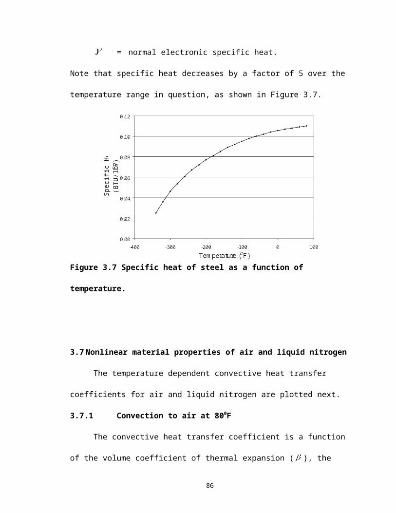
Figure 4.28a Plot results.
Figure 4.28b Contour plot.
Repeat Step 1 to Step 3 to view different quantities at different or the same times.
101
Pick the quantitythat needs to be plotted.
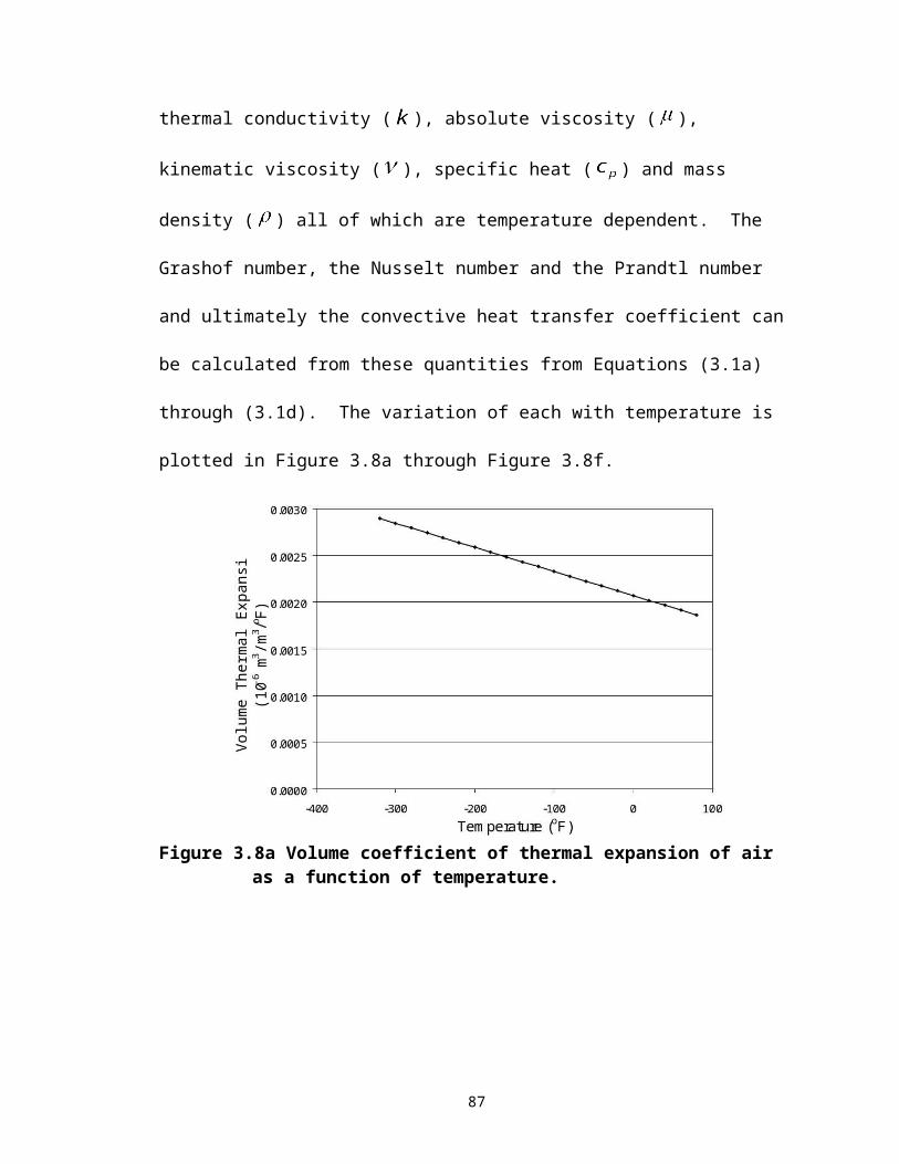
4.5.4 Plotting parts of the assembly
Contour plots of individual parts of the assembly can be plotted by
choosing them on the ANSYS toolbar as shown in Figure 4.29.
Figure 4.29 ANSYS toolbar (choose part of interest).
Follow steps 1-3 of the general postprocessor described in Section 4.5. Once you are
finished with the General Postprocessor click ALL on the ANSYS toolbar to select all
entities
4.6 Time history postprocessor
The time history postprocessor plots variables against time. The THGTM has
been programmed to plot hoop stress, temperature and critical crack length versus time.
Prior to performing the steps described next the user should have either:
1. Performed a run of the program (Step 1 to Step 20) in Section 4.3, and
click on DIMSET on the ANSYS toolbar, or
2. Resumed a previous run (Step 1 to Step 3) of Section 4.4.
102
Choosing parts of the assembly
Select all entities
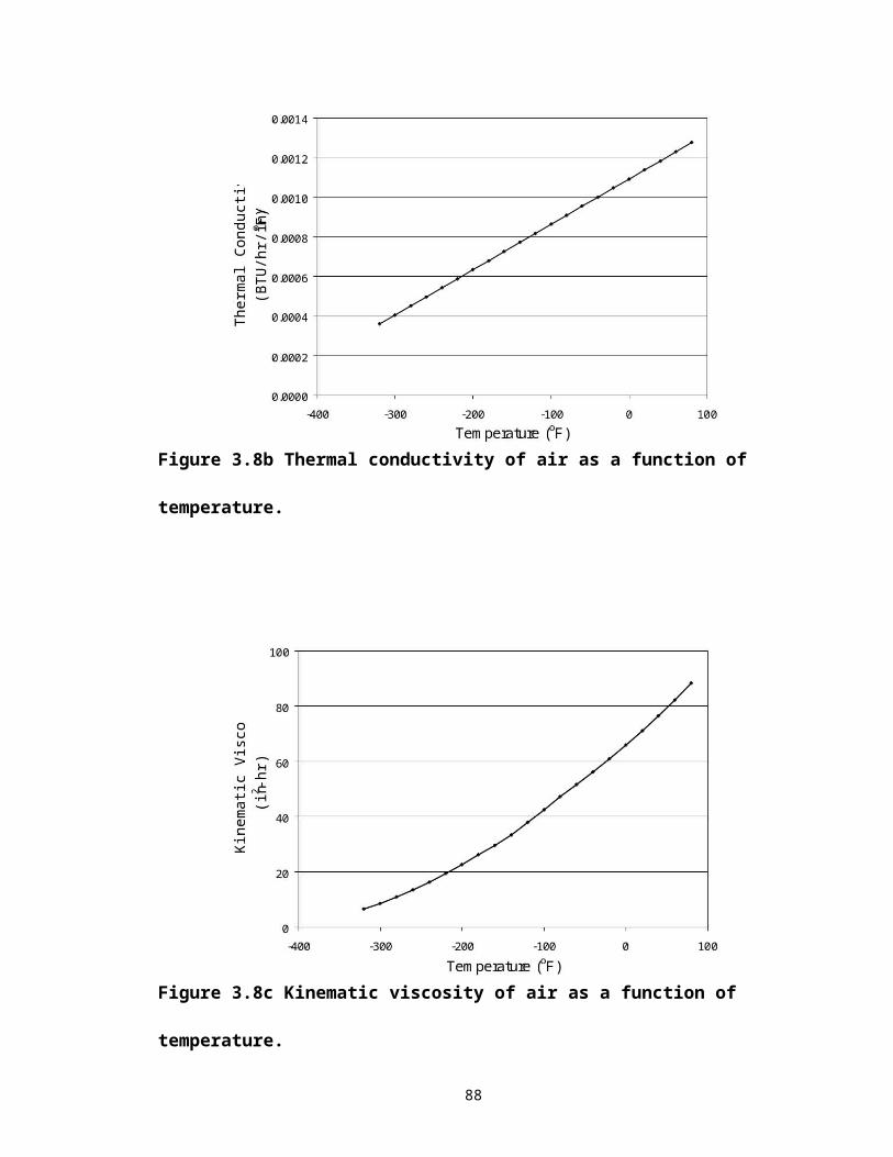
4.6.1 Step 1
On the ANSYS toolbar shown in Figure 4.30 click on TIMEHIS.
Figure 4.30 ANSYS toolbar (time history postprocessor).
4.6.2 Step 2
You will get a dialog box like the one shown in Figure 4.31a.
Figure 4.31a Enter part of interest.
Enter ‘t’ for trunnion, ‘h’ for hub and ‘g’ for girder. The requested part of the assembly
with the elements attached to it is plotted. The working of the time history postprocessor
is explained with the help of an example. For example, if ‘h’ is entered, the elements
attached to the hub are plotted as shown in Figure 4.31b.
103
Click here
Trunnion is the default
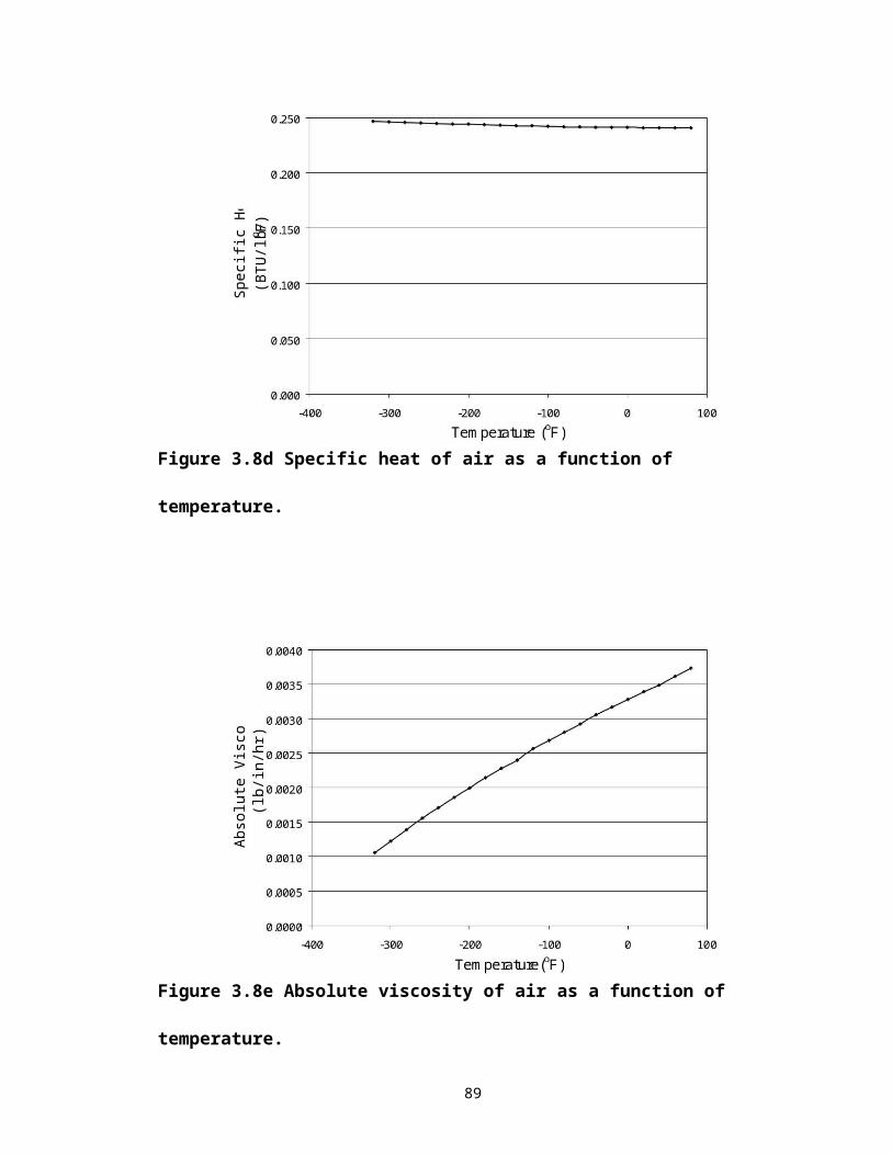
Figure 4.31b Selected component.
A pick menu shown in Figure 4.31c also appears.
104
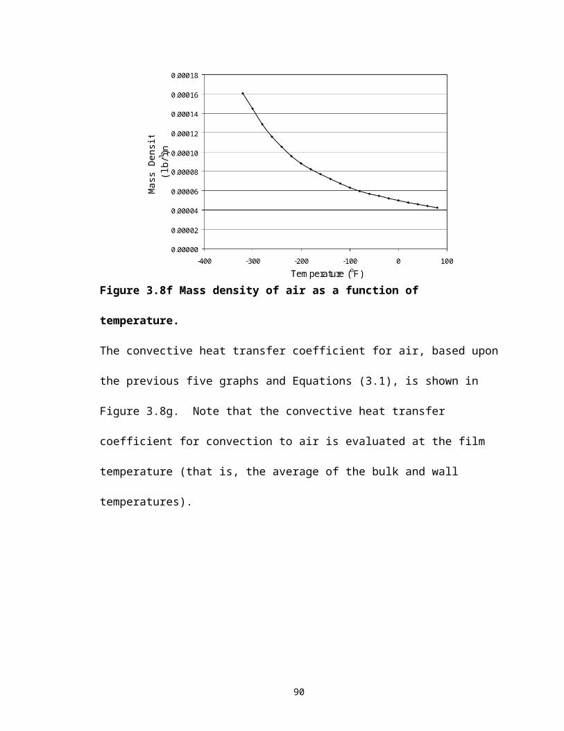
Figure 4.31c Pick elements.
If we move the cursor over the ANSYS Graphics window the pick arrow points
upwards indicating that we are in a pick mode. The desired element can be ‘picked’ by
left clicking the mouse over it and Clicking OK. However, in practice it is often difficult
to click at the right location and often misplaced clicks result in the wrong element being
selected. A technique described next will help the user pick the correct element. The
previous example is continued here.
4.6.3 Step 3a
Go to the Utility Menu and enter the following.
Utility Menu>PlotCtrls>Pan, Zoom, Rotate
The Pan-zoom-rotate menu shown in Figure 4.32 appears on the screen.
105
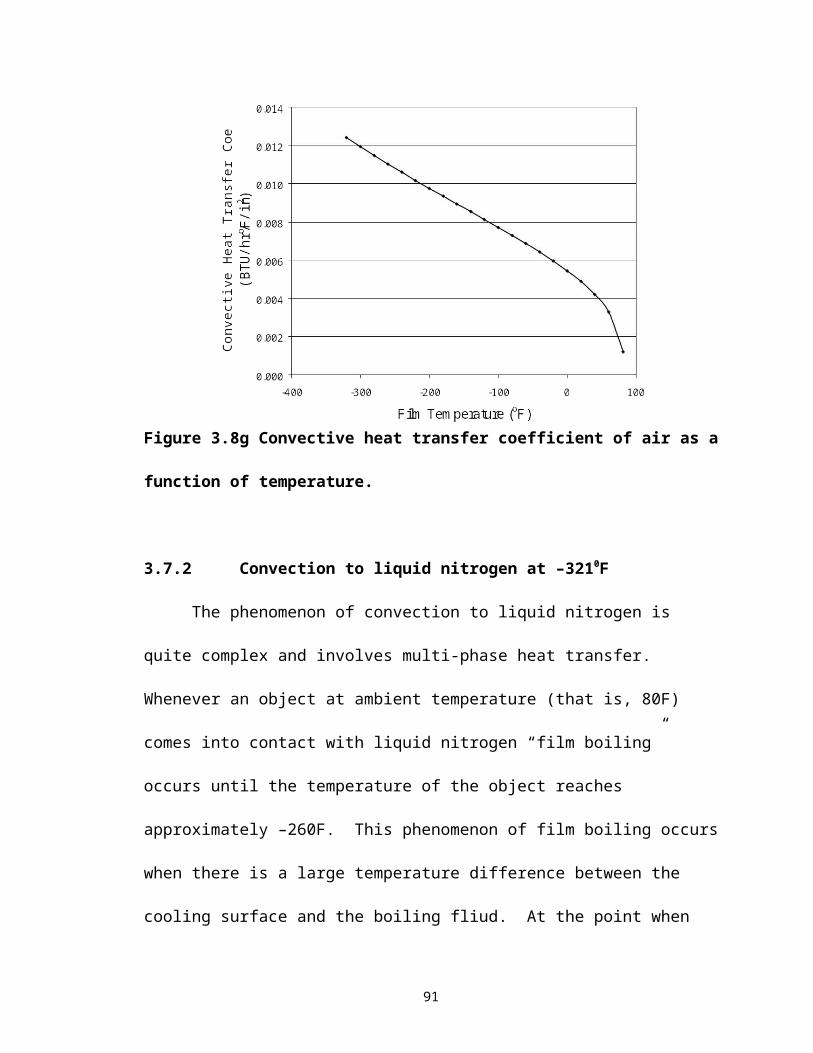
Figure 4.32 Pan-zoom-rotate.
4.6.4 Step 3b
Click ‘Front’ in Figure 4.32 and choose the element which has the same radial
and hoop co-ordinates of our point of interest as shown in the Figure 4.33
106
Click here
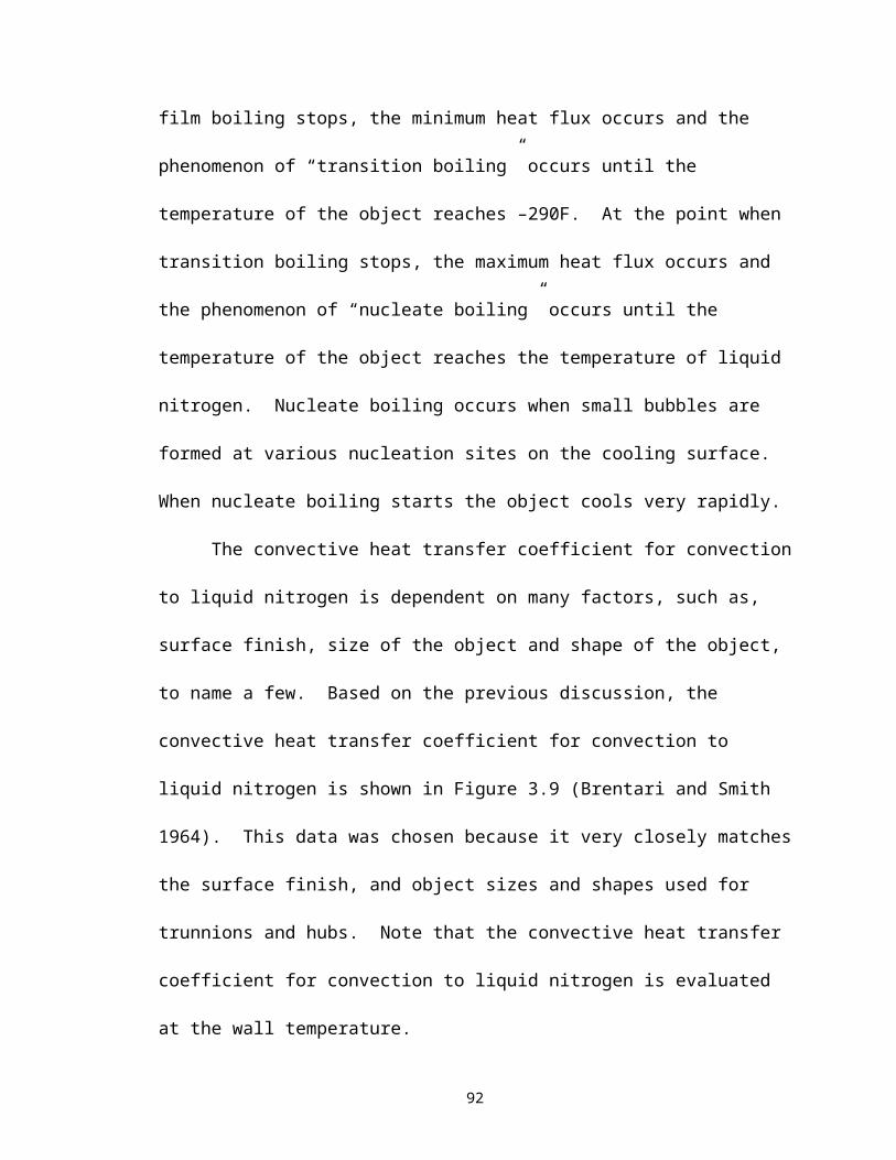
Figure 4.33 Front view.
4.6.5 Step 3c
Click ‘Right’ on the pan, zoom and rotate dialog box in Figure 4.32 and the right view of
the part in question appears as shown in Figure 4.34.
107
Click here
Figure 4.34 Right view.
4.6.6 Step 3d
If there is more than one element with the same r and co-ordinate then the
dialog box similar to the one shown in Figure 4.35 will appear on the screen.
Figure 4.35 Multiple entities.
108
Keep clicking next till the element with the z coordinate of interest is picked
Click here
Each time you click the next element with same z co-ordinate is chosen. Continue
clicking till the element of interest is chosen. Then click OK on the ‘reselect elements’
menu.
In case you select the wrong element, you can enter the unselect mode by a right
mouse click. After unselecting the unwanted element, you can enter the select mode
again by right clicking again.
4.6.7 Step 3e
On clicking OK the element chosen is plotted. The view of the element can be
changed using the Pan Zoom and Rotate. A dialog box similar to the one shown in
Figure 4.36a appears.
Figure 4.36a Pick nodes.
109
Select the node of choice by clicking near it on the ANSYS Graphics window and
clicking OK. In case you select the wrong node you can enter the unselect mode by a
right mouse click. After unselecting the unwanted node you can enter the select mode
again by right clicking again.
It will take some time for the results to appear on the screen. Wait for the
hourglass on the screen to disappear. A graph similar to the one shown in Figure 4.36b
appears on the screen.
Figure 4.36b Time history plot.
110
To print the graph, enter the following.
Utility Menu>Plot Ctrls>Hard Copy> to printer
To save the graph, enter the following.
Utility Menu>Plot Ctrls>Hard Copy>to file
The graph is saved as a bitmap file (*.bmp) in the working directory.
4.6.8 Options
To list the results, on the ANSYS toolbar shown in Figure 4.37a, click on HTLIST.
Figure 4.37a ANSYS toolbar (list results).
The results are listed in the format shown in Figure 4.37b
Figure 4.37b Time history listing.
The pull down menus allow you to save and print the listing.
111
Click here
To save the listing
To print the listing
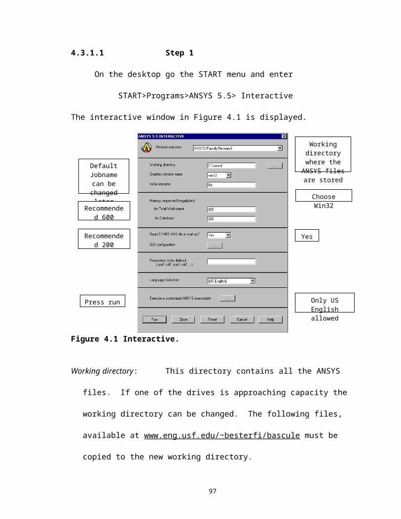
CHAPTER 5
RESULTS AND CONCLUSIONS
5.1 Introduction
The results of the study are presented in this chapter. Theories of failure based on
fracture mechanics and yield stresses present several alternative causes of failure. The
relevant theory for crack formation in the Trunnion-Hub-Girder (THG) was formulated
based on several observations. First, the steady state stresses after assembly were well
below the yield point and could not have caused failure. Second, the brittle nature of the
material (ASTM A203-A) ruled out failure due to Von Mises stresses. Third,
experimental observations indicate the presence of small cracks in the assembly. Last,
cracks were formed during the immersion of the trunnion-hub assembly in liquid
nitrogen. This observation is important as fracture toughness decreases with a decrease
in temperature whereas yield strength increases with a decrease in temperature. Our
hypothesis is that the small cracks present in the assembly propagate catastrophically
once the size of the crack exceeds the critical crack length. This hypothesis is tested
using the THGTM (Trunnion-Hub-Girder Testing Model). A brief explanation of this
theory is included.
Time history plots of temperatures, hoop stresses and critical crack lengths at
different stages in the assembly process are presented. The plots show the
interdependence of the variables and suggest possible avenues of optimizing them by
changing the parameters or steps involved in the assembly process. One possible
112
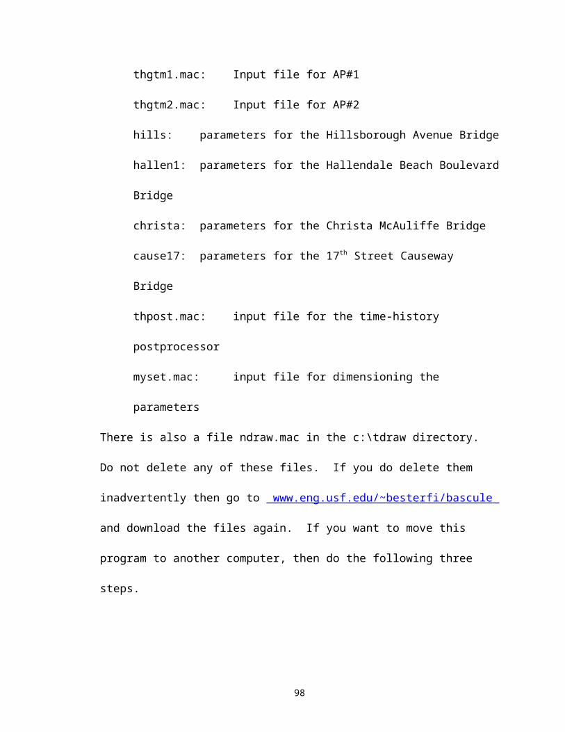
solution, using AP#2 (see Section 2.3.2), is explored and a comparison between the two
assembly procedures for different bridges is presented. A phenomenon called crack
arrest, that may prevent cracking in some cases despite low critical crack lengths, is
described and the possibility of it occurring is explored.
The results are important from two perspectives, one of which is explicitly
presented in the results and the other which is implicitly suggested. The explicit result is
the comparison between the two assembly procedures. Also, implicitly presented in the
results is a comparison of different bridges explaining why some THG assemblies form
cracks while others do not.
5.2 Bridge geometric parameters
The geometric parameters for the three bridges, that is, Christa McAuliffe Bridge,
Hillsborough Avenue Bridge and 17th Street Causeway Bridge, are presented in Table
5.1a. For a schematic and description of the parameters, refer to Figures 4.13a, 4.13b,
4.14a, 4.14b, 4.15a and 4.15b of Chapter 4.
Interference values for FN2 fits can be obtained from the Bascule Bridge Design
Tools (Denninger, 2000) by approximating the THG assembly to be three long concentric
annular cylinders. In this study, we analyze the worst case, that is, maximum interference
between the trunnion and hub and minimum interference between the hub and the girder.
These values of interference will cause the largest tensile hoop stress in the hub. The
interference values, based on FN2 fits, used in this analysis are presented in Table 5.1b.
113
Table 5.1a Geometric parameters.
GEOMETRIC PARAMETERS
BRIDGECHRISTA
MCAULIFFEHILLSBOROUGH
AVENUE17TH STREET CAUSEWAY
hgf (in) 1.5 1 0.75hgw (in) 82 90 60
l (in) 18.5 20 6lf (in) 4.25 8.5 4.25lg (in) 82 90 60lh (in) 16 22 11lt (in) 53.5 62 23
rhg (in) 16 15.39 8.88rho (in) 27 24.5 13.1825rti (in) 1 1.125 1.1875rto (in) 9 8.39 6.472tg (in) 1.5 1.5 1.25
wbr (in) 1.75 1.75 0.78125wgf (in) 17 14 1.25wgw (in) 1.5 1 0.75whf (in) 1.75 1.75 1.25
Table 5.1b Interference values.
DIAMETRICALINTERFERENCE
BRIDGECHRISTA
MCAULIFFE
HILLSBOROUGH
AVENUE
17TH STREETCAUSEWAY
Trunnion-Hub (in)
0.008616 0.008572 0.007720
Hub-Girder (in) 0.005746 0.005672 0.004272
5.3 Bridge loading parameters
The material properties of an equivalent metal, that is, Fe - 2.25 Ni (ASTM
A203-A), are presented in Chapter 3. Also presented are the thermal properties of air and
liquid nitrogen. Bulk temperatures used for the results presented are given in Table 5.2.
Table 5.2 Bulk temperatures.TYPE OF BULK TEMPERATURE TEMPERATUR
EAmbient air bulk temperature 85 0FCooing medium bulk temperature -321 0F
114
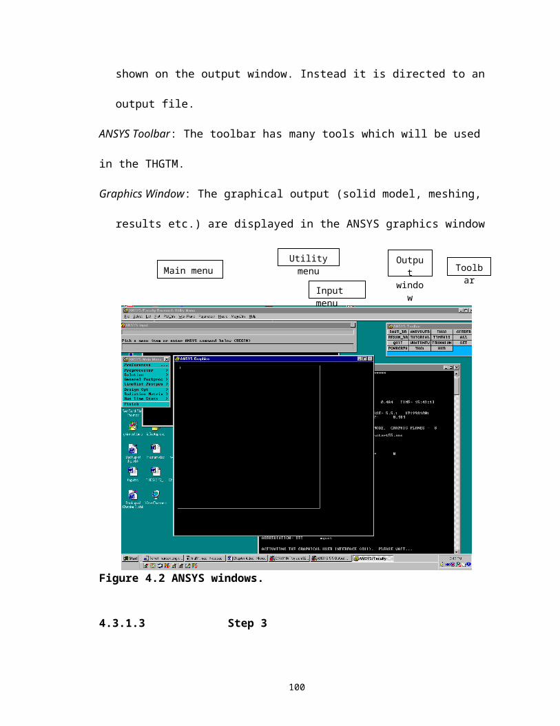
5.4 Convergence test and result verification
A convergence test is performed to verify the suitability of the mesh used in the
analysis. The hoop stress is calculated at different levels of meshing, that is, different
mesh densities. The hoop stress, , at a point (Logan, 1992) is given by
(5.1a)
where
B and = constants,
A = extrapolated result for infinite mesh density, and
N = number of elements.
Note that as N , 0, A for >1. So, for >1 the results will
converge and for <1 the results will diverge. Table 5.3a show the results with different
mesh densities (that is, 3096, 4740 and 6336 elements).
Table 5.3a Results with different mesh densities.NUMBER OF ELEMENTS,
NHOOP STRESS (ksi)
3096 27.3284740 31.1586336 32.686
Using the information from Table 5.3a and Equation (5.1a) results in the
following three simultaneous equations in terms of A, B and .
=27.328= (5.1b)
115
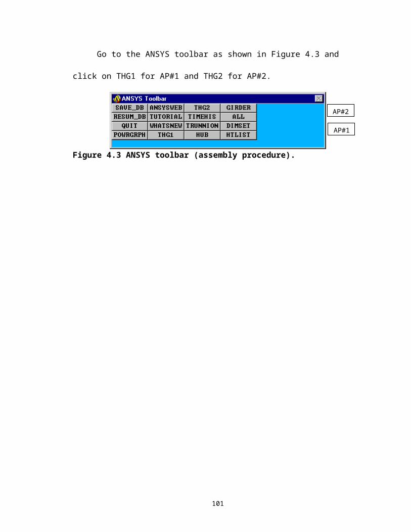
=31.158= (5.1c)
=32.686= (5.1d)
Solving Equations (5.1a) through (5.1c) for A, B and yields A=35.551 ksi, B=1.133 x
109, and =1.472208. Since >1, the results will converge.
A comparison of stresses at steady state at the inner radius of the hub with those
obtained from the Bascule Bridge Design Tools (BBDT) (Denninger, 2000) is presented
in Table 5.3b.
Table 5.3b Comparison between trunnion-hub-girder testing model and bascule bridge design tools results.
BRIDGESTRESS (ksi) PERCENT
DIFFERENCETHGTM BBDTChrista McAuliffe 9.812 9.372 4.59 %Hillsborough Avenue 10.173 9.813 3.62 %17th Street Causeway 14.298 13.457 6.06 %
The results are within an allowable difference, especially considering that the geometries
in the BBDT are approximated to long annular cylinders.
5.5 Hoop stress, temperature and critical crack length
Our hypothesis is that small cracks present in the assembly propagate
catastrophically once they attain a critical crack length, . The critical crack length is
determined by the Equation (5.2) (Kanninen and Popelar, 1985).
(5.2)
where
= critical crack length,
= temperature dependent critical stress intensity factor,
116
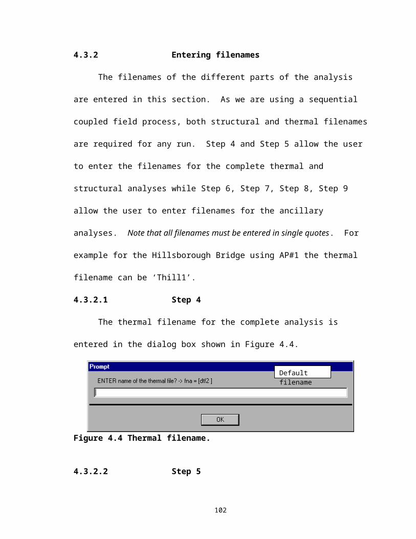
= edge effects, and
= hoop stress.
The critical crack length is dependent upon the fracture toughness, , and
the hoop stress, . The critical stress intensity factor, , in turn is a function of
temperature. decreases with an decrease in temperature as shown in Figure 5.1 (.
Figure 5.1 Fracture toughness and temperature.
Our hypothesis is that in AP#1, a combination of high hoop stress and low
temperature result in smaller values of critical crack length, possibly leading to crack
formation. In AP#2, stresses due to interference never occur together with the thermal
stresses during the cooling process, possibly resulting in larger values of critical crack
length, thereby reducing the probability of crack formation. In short, temperature, hoop
stress and critical stress intensity factor (fracture toughness) are not optimized in AP#1
and AP#2 may resolve this problem. A multiplicity of factors (geometry, temperature
dependent material properties, thermal stresses, interference stresses, etc.) affect the
117

stresses in the assembly with some parameters sometimes reinforcing and yet at other
times negating the effects of each other. Therefore, this intuitive analysis needs to stand
the test of a numerical model before gaining engineering acceptability. The THGTM is
used for this purpose.
The THGTM is used to plot the temperature, hoop stress and the critical crack
length at possible points of failure in the assembly. The critical crack length is used as
the parameter for comparison between different assembly procedures for different
bridges. A further study possible with the THGTM (though not included as a part of this
study) is analyzing the effect of the different loading parameters on the critical crack
length.
5.5 Transient stresses and critical crack length using the trunnion-hub-girder testing model
The THGTM is used to analyze the stresses and critical crack length at possible
locations of failure. We choose the point with the greatest probability of failure and plot
critical crack lengths, hoop stress and temperature against time for that point.
With the aim of modeling the worst case from the perspective of failure (see
Section 5.12) in our model, the male parts of the assembly are inserted into the female
parts as soon as the interference between the two is breached. In practice, it is often
difficult to shrink-fit an assembly without an clearance, and hence the high stresses after
contact may not be observed in practice. It is important to note that in practice it is
impossible to perform an insertion without a gap and hence the high stresses noticed
immediately after contact may not be observed in practice. Also, the entire assembly
process and the ancillary cooling processes are performed separately. Hence, the time
periods for which the cooling is performed in the full assembly process (only till
118
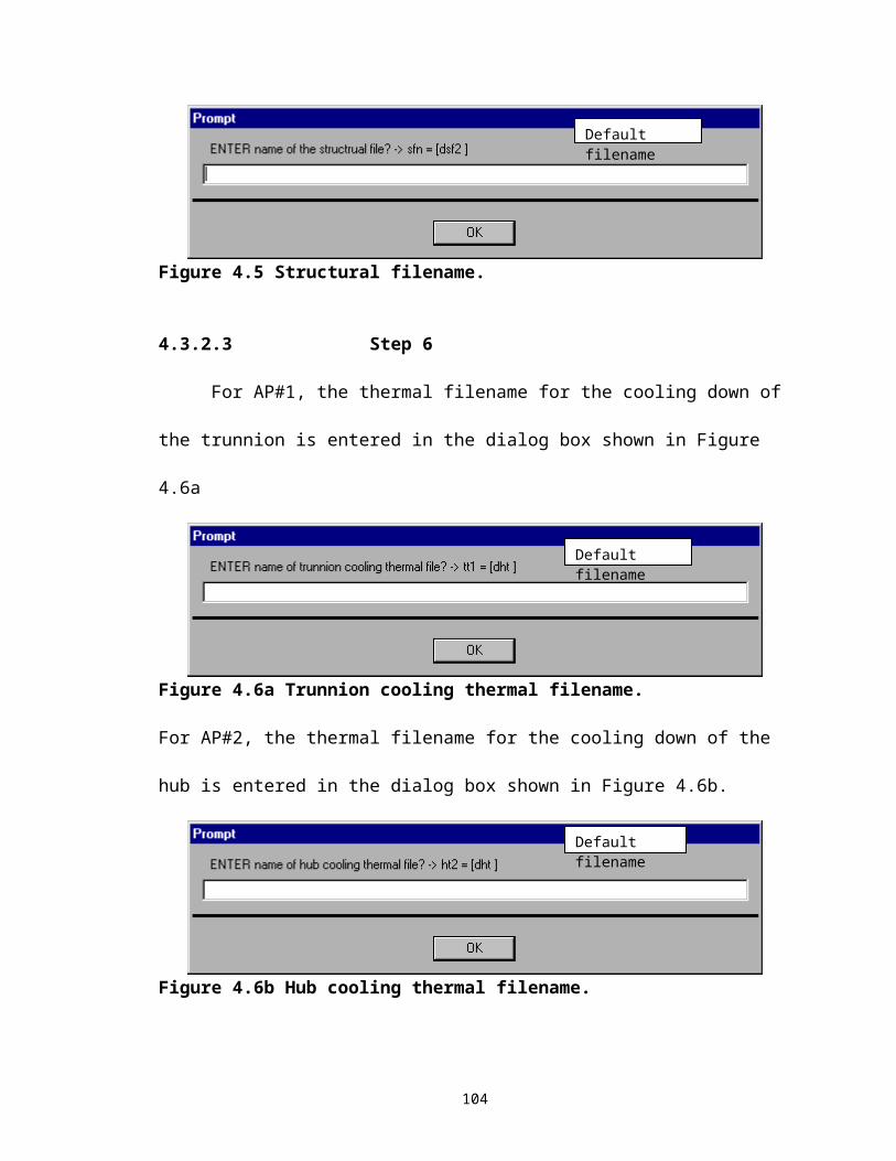
interference is breached) will be different from that in the ancillary cooling process (user
specified cooling time).
The results are presented with time-history plots for all the bridges. Selected
contour plots are presented only for the Christa McAuliffe Bridge.
5.7 Christa McAuliffe Bridge
Possible critical points in the hub are studied using the THGTM. The element at
the inner radius of the hub on the gusset side is found to be the most critical element.
Figure 5.2 shows the chosen element.
Figure 5.2 Front and side view of the chosen element in the Christa McAuliffe hub.
5.7.1 Assembly procedure 1 (AP#1)
5.7.1.1 Full assembly process
The stresses, temperatures and critical crack lengths during AP#1 are plotted
against time in Figure 5.3. The time period for which each step of the assembly process
is performed is given in Table 5.4.
119
Element
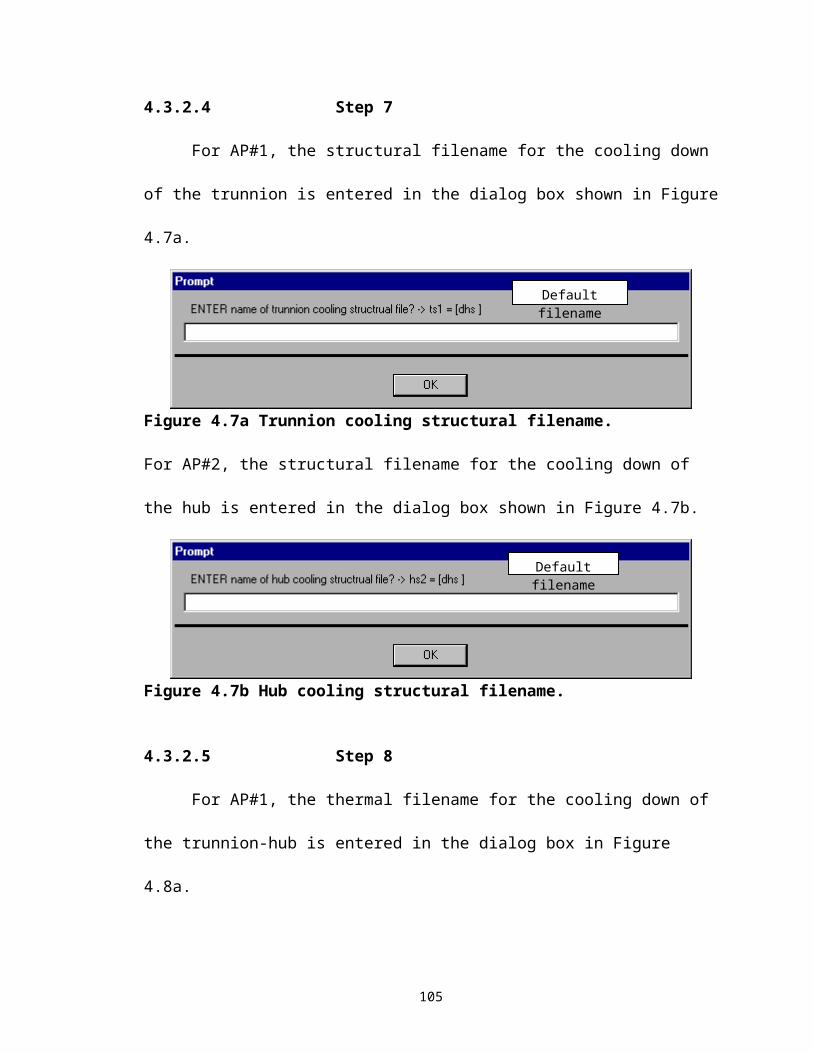
Figure 5.3 Critical parameters plotted against time (full assembly process during AP#1 of Christa McAuliffe Bridge).
Table 5.4 Time for each step of AP#1 for the Christa McAuliffe Bridge.
STEPSTARTIN
GTIME
ENDING
TIMECooling down of the trunnion (min) 0 3Sliding the trunnion into the hub (min) 4 503Cooling down the trunnion-hub assembly (min) 504 505Sliding the trunnion-hub assembly into the girder (min) 506 1705
120
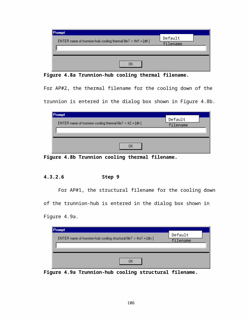
5.7.1.2 Cooling down of the trunnion
The stresses at the hub are not affected during this step.
5.7.1.3 Sliding the trunnion into the hub
The hoop stress, temperature and the critical crack length during this step are
plotted against time in Figure 5.4. Almost immediately after contact, a combination of
interference and thermal stresses produces high hoop stresses at the inner radius of the
hub. Due to the effects of conduction and convection, the temperatures in the trunnion-
hub assembly begin to converge to around the same temperature. As a consequence, the
thermal stresses play an increasingly marginal role with the passage of time.
Figure 5.4 Critical parameters plotted against time (sliding the trunnion into the hub during AP#1 of the Christa McAuliffe Bridge).
Though this step is not important from the perspective of failure, as the critical
crack lengths are high, an interesting interplay of temperatures, hoop stresses and critical
121
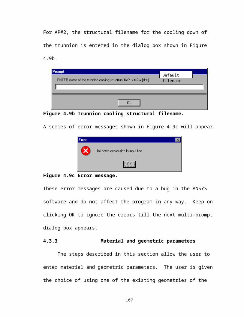
crack length can be seen. As temperature and hoop stress fall, the critical crack length
initially falls before rising. (see Equation (5.2))
5.7.1.4 Cooling down the trunnion-hub assembly
The hoop stress, temperature and the critical crack length during this step are
plotted against time in Figure 5.5a. The results from the THGTM indicate that the lowest
values of critical crack length during AP#1 are observed during this step. This result is
supported by experimental observation of crack formation during this step (see Section
1.1). This assumes special significance as Christa McAuliffe is one of the bridges that
formed cracks during this step. Furthermore, the critical crack length remains low for a
considerable period of time in contrast to what is observed in AP#2 during its counterpart
critical step: cooling of the hub (see Section 5.7.2.2). This behavior assumes importance
in our discussion of crack arrest (see Section 5.11). Initially, thermal and interference
stresses reinforce each other and high hoop stresses occur as a result. As the trunnion-
hub assembly nears steady state, the stresses due to interference dominate.
122
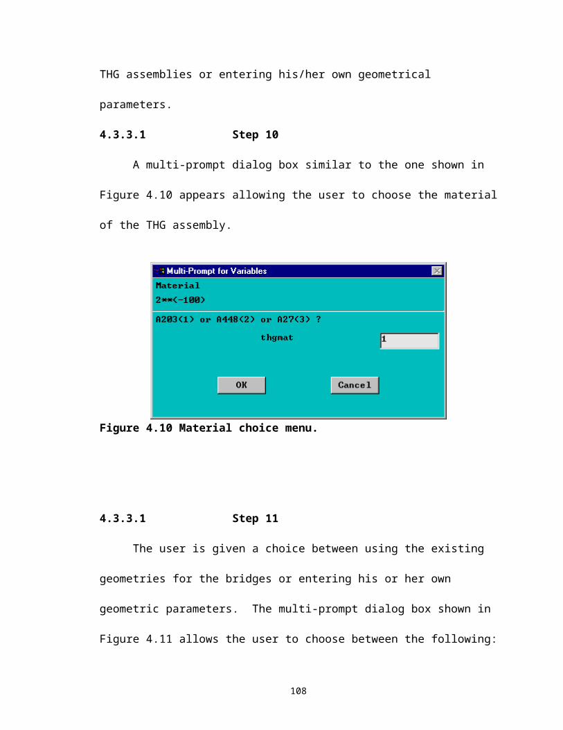
Figure 5.5a Critical parameters plotted against time (cooling down of the trunnion-hub assembly during AP#1 of the Christa McAuliffe Bridge).
Contour plots of the hoop stress and the temperature in the hub when the highest
hoop stress is noticed are plotted in Figures 5.5b and 5.5c, respectively. Hoop stress and
temperature plots when the lowest critical crack is observed are plotted in Figures 5.5d
and 5.5e, respectively.
123

Figure 5.5b Hoop stress plot when the highest hoop stress during AP#1 is observed.
Figure 5.5c Temperature plot when the highest hoop stress during AP#1 is observed.
124
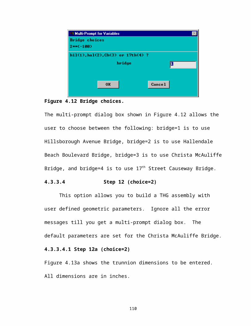
Figure 5.5d Hoop stress plot when the lowest critical crack length during AP#1 is observed.
Figure 5.5e Temperature plot when the lowest critical crack length during AP#1 is observed.
125
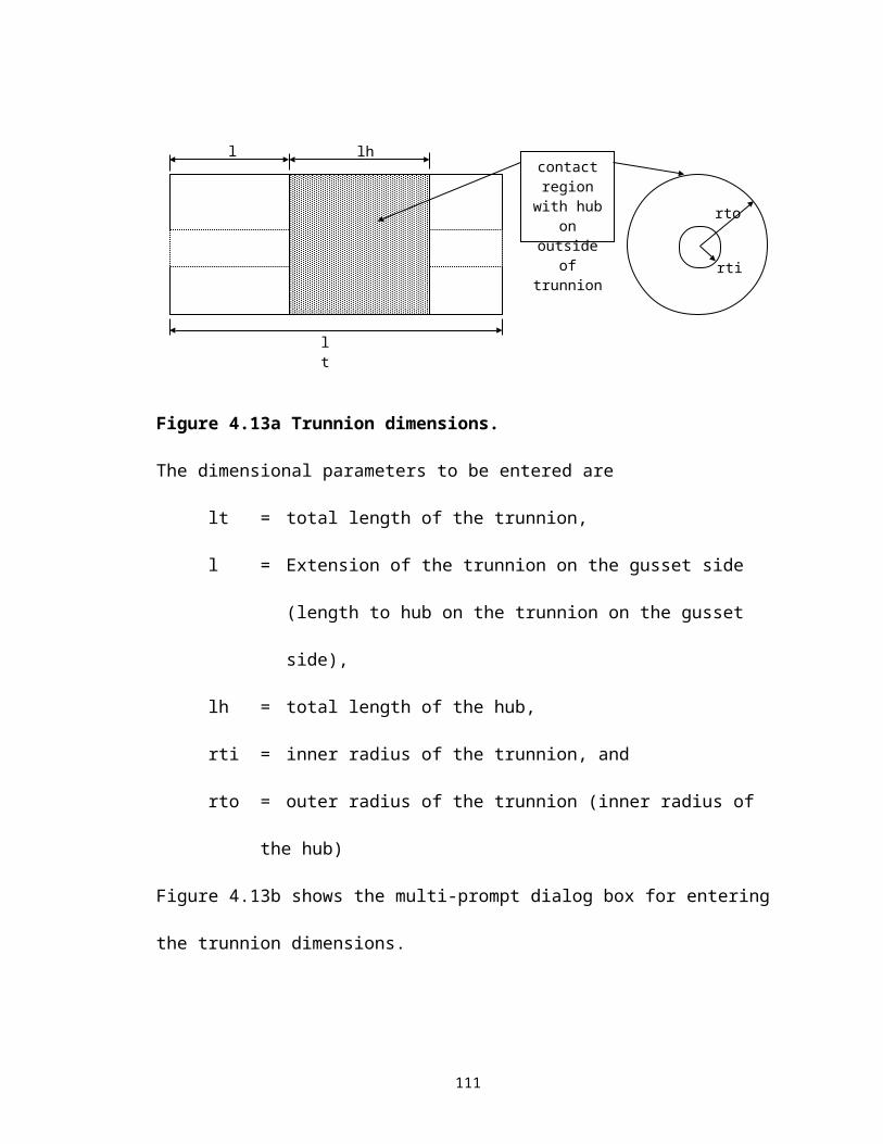
5.7.1.5 Sliding the trunnion-hub assembly into the girder
The hoop stress, temperature and the critical crack length during this step are
plotted against time in Figure 5.6 for this step. During this step, hoop stresses remain
fairly stable primarily due to the remoteness of the inner radius of the hub from the hub
girder interface. A rise in the temperature due to conduction and convection is
accompanied initially with a rise, and later a fall in the hoop stress, confirming the
somewhat non-intuitive behavior of thermal stresses. High values of the critical crack
length indicate the low probability of crack propagation during this step.
Figure 5.6 Critical parameters plotted against time (sliding the trunnion–hub assembly into the girder during AP#1 of Christa McAuliffe Bridge).
126
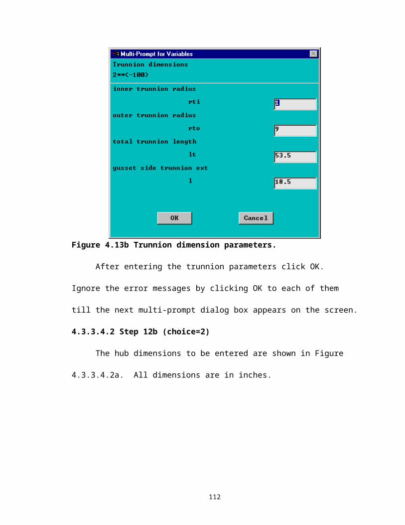
5.7.2 Assembly Procedure 2 (AP#2)
5.7.2.1 Full assembly process
The stresses, temperatures and critical crack lengths at the chosen element are
plotted against time in Figure 5.7. The time period for which each step of the assembly
process is performed is given in Table 5.5.
Figure 5.7 Critical parameters plotted against time (full assembly process during AP#2 of Christa McAuliffe Bridge).
Table 5.5 Time for each step of AP#2 for the Christa McAuliffe Bridge.
STEPSTARTIN
GTIME
ENDING
TIMECooling down of the hub (min) 0 2Sliding the hub into the girder (min) 3 202Cooling down the trunnion (min) 203 208Sliding the trunnion into the hub-girder assembly (min) 209 2158
127
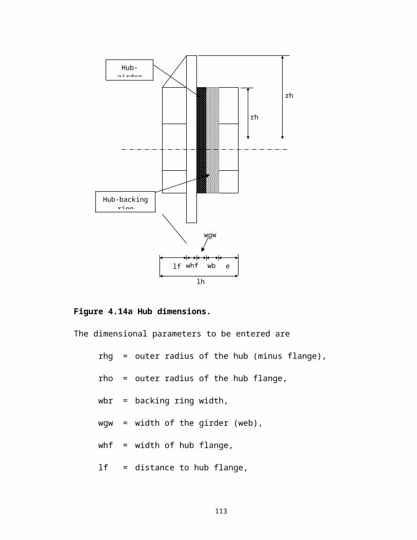
5.7.2.2 Cooling down of the hub
The stresses, temperatures and critical crack lengths during this step are plotted
against time in Figure 5.8a. A sharp thermal gradient across the radius in inner radius of
the hub initially results in high values of hoop stress. Over time, as the temperature
gradient becomes less steep, the hoop stresses fall. The lowest value of critical crack
length in AP#2 is observed during this step. Note that the critical crack length rises
almost instantaneously after reaching its lowest point indicating a possibility of crack
arrest (see Section 5.11)
Figure 5.8a Critical parameters plotted against time (cooling down of the hub during AP#2 of the Christa McAuliffe Bridge).
Contour plots of the hoop stress and the temperature in the hub when the highest hoop
stress is noticed are plotted in Figures 5.8b and 5.8c, respectively. Hoop stress and
128
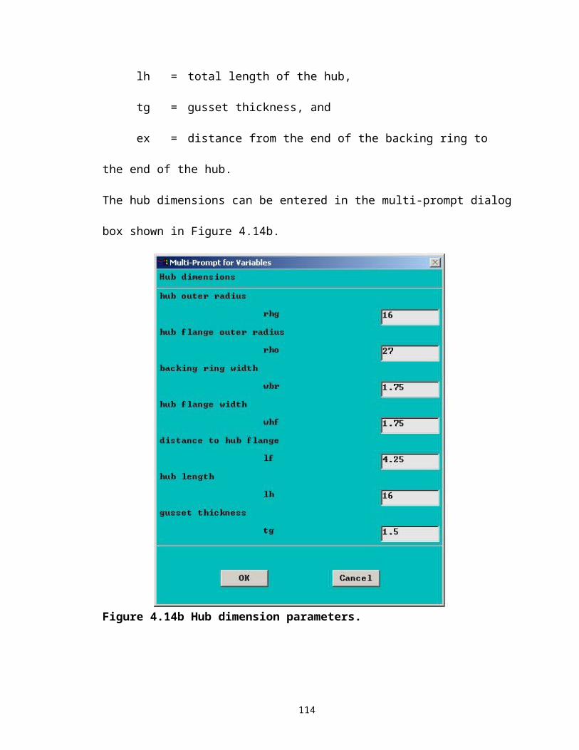
temperature plots when the lowest critical crack is observed are plotted in Figures 5.8d
and 5.8e, respectively.
Figure 5.8b Hoop stress when the highest hoop stress during AP#2 is observed.
Figure 5.8c Temperature plot when the highest hoop stress during AP#2 is observed.
129

Figure 5.8d Hoop stress when the lowest critical crack length during AP#2 is observed.
Figure 5.8e Temperature plot when the lowest critical crack length during AP#2 is observed.
130
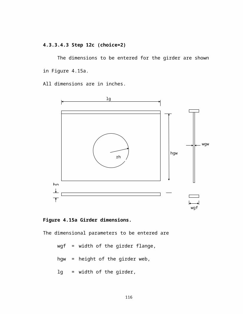
5.7.2.3 Sliding the hub into the girder
The stresses, temperatures and critical crack lengths during this step are plotted
against time in Figure 5.9. The hoop stresses during this step are compressive. The
critical crack length is not defined for compressive hoop stresses, and hence, is shown as
zero. The relatively low values of compressive hoop stress are explained by the
remoteness of the inner radius of the hub from the hub-girder interface.
Figure 5.9 Critical parameters plotted against time (sliding the hub into the girder during AP#2 of the Christa McAuliffe Bridge).
5.7.2.4 Cooling down of the trunnion
The stresses in the hub are not affected during the cooling of the trunnion.
5.7.2.5 Sliding the trunnion into the hub-girder assembly
The stresses, temperatures and critical crack lengths during this step are plotted
against time in Figure 5.10.
131
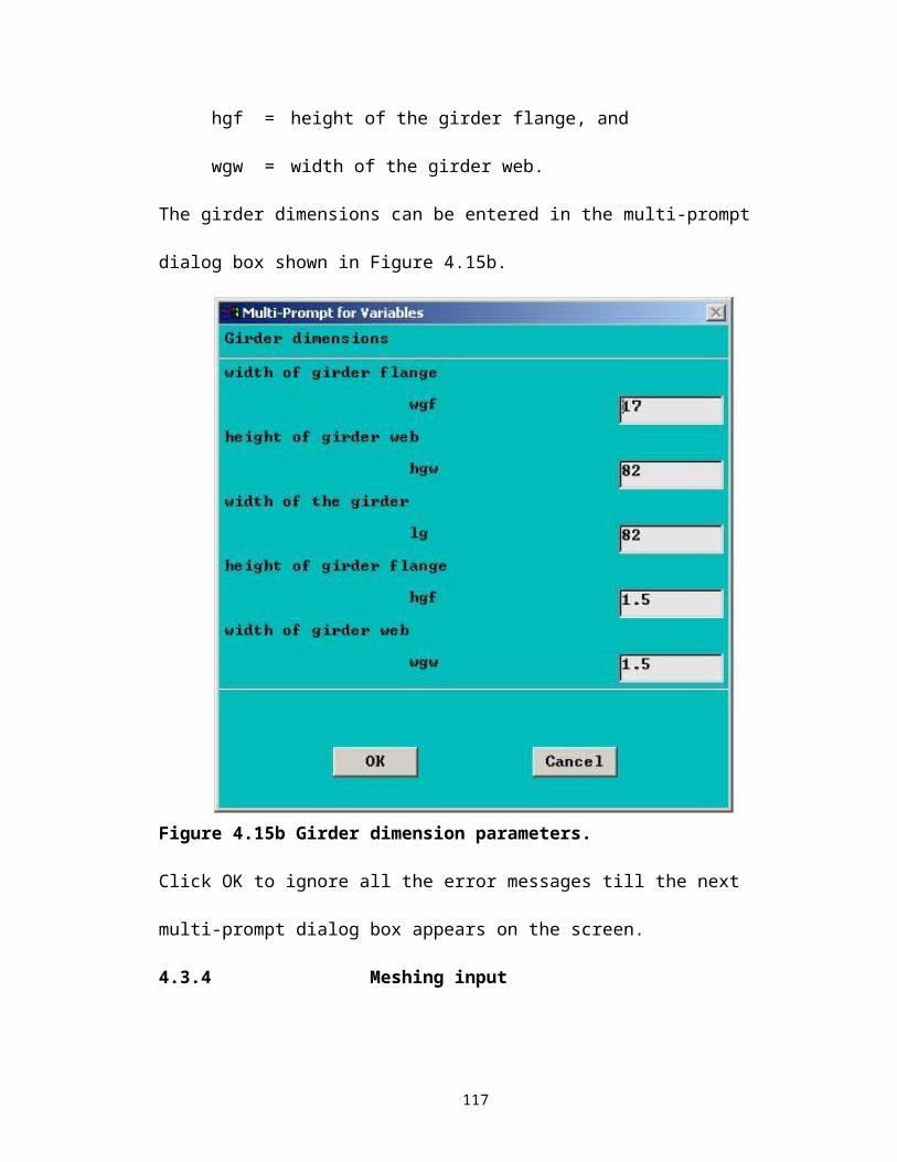
Almost immediately after contact, a combination of thermal stresses due to the
sharp thermal gradient and interference stresses result in high hoop stresses. Over time,
due to the effects of conduction and convection, the temperatures in the assembly begin
to converge and interference stresses become dominant. High values of critical crack
length indicate low probability of failure.
Figure 5.10 Critical parameters plotted against time (sliding the trunnion into the hub-girder assembly during AP#2 of the Christa McAuliffe Bridge).
132
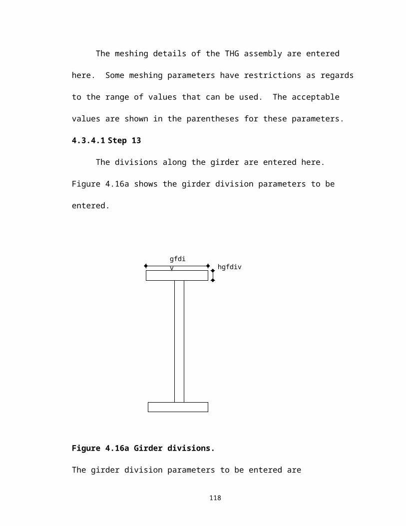
5.8 Hillsborough Avenue Bridge
Possible critical points are studied in the hub using the THGTM. The element at
the inner radius of the hub on the backing ring side is found to be the most critical.
Figure 5.11 shows the chosen element in the hub.
Figure 5.11 Front and side view of the chosen element in the Hillsborough Avenue hub
5.8.1 Assembly procedure 1 (AP#1)
5.8.1.1 Full assembly process
The hoop stresses, temperatures and critical crack lengths at the chosen element
are plotted against time in Figure 5.12. Time period for each step of the assembly
process is performed is listed in Table 5.6.
133
Element
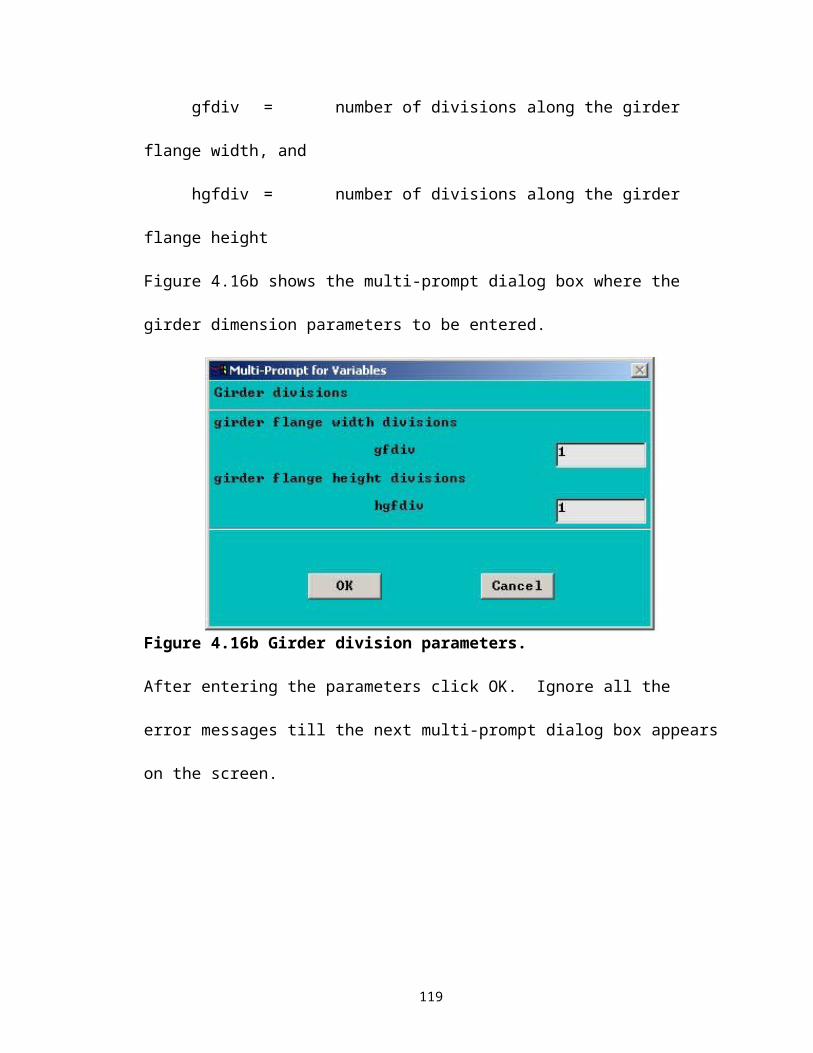
Figure 5.12 Critical parameters plotted against time (full assembly process during AP#1 of the Hillsborough Avenue Bridge).
Table 5.6 Time for each step of AP#1 for the Hillsborough Avenue Bridge.
STEPSTARTIN
GTIME
ENDING
TIMECooling down of the trunnion (min) 0 3Sliding the trunnion into the hub (min) 4 2603Cooling down the trunnion-hub assembly (min) 2604 2605Sliding the trunnion-hub assembly into the girder (min) 2606 4805
5.8.1.2 Cooling down of the trunnion
The stresses in the hub are not affected during the cooling down of trunnion.
5.8.1.3 Sliding the trunnion into the hub
The hoop stresses, temperatures and the critical crack lengths during this step are
plotted against time in Figure 5.13.
134
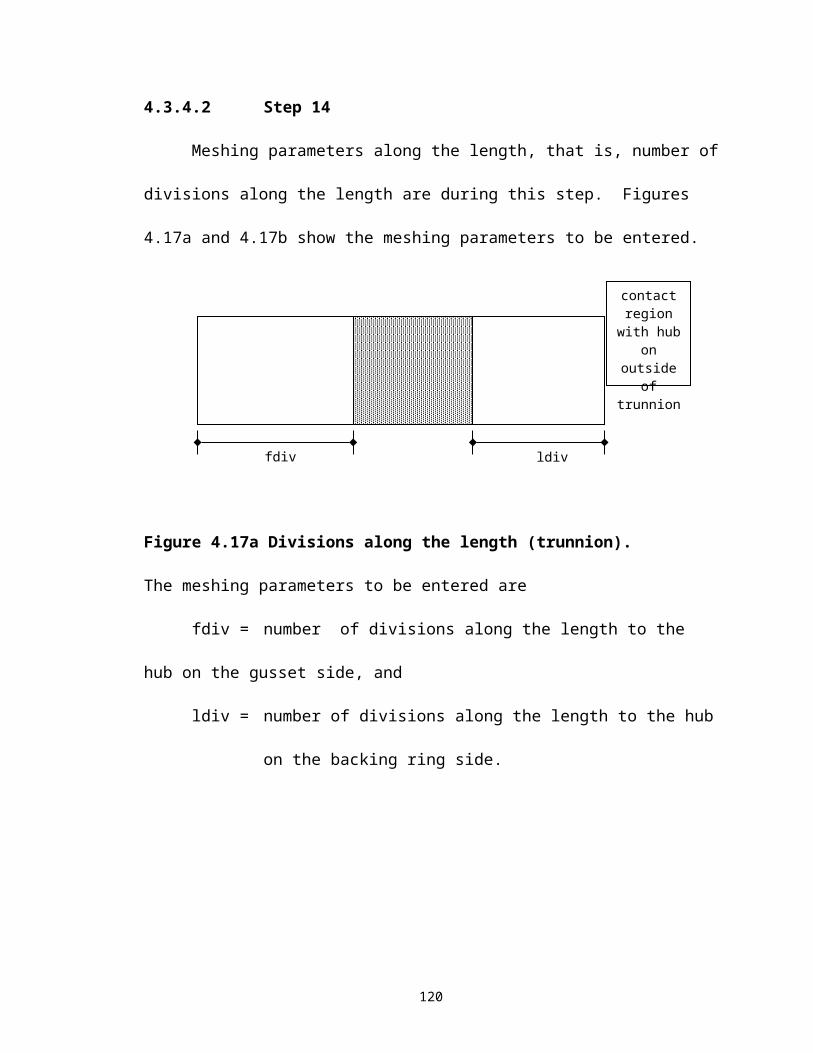
A combination of stresses due to a sharp thermal gradient and interference
stresses result in high hoop stresses after contact. As the temperature in the assembly
becomes constant due to the effects of conduction and convection, stresses due to
interference dominate. High values of critical crack length indicate low probability of
failure.
Figure 5.13 Critical parameters plotted against time (sliding the trunnion into the hub during AP#1 of the Hillsborough Avenue Bridge).
5.8.1.4 Cooling down the trunnion-hub assembly
The hoop stress, temperature and the critical crack length during this step are
plotted against time in Figure 5.14. The results from the THGTM indicate that the lowest
values of critical crack length during AP#1 are observed during this step. Initially,
thermal and structural stresses reinforce each other and high hoop stresses occur as a
result. As the trunnion-hub assembly nears steady state, the stresses due to interference
135
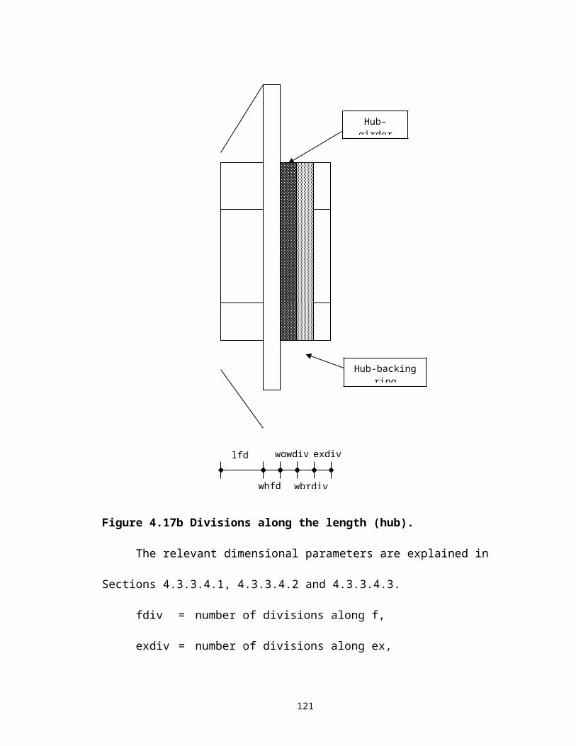
dominate. The trends of stresses and critical crack length are similar to what is observed
in the Christa McAuliffe Bridge. The critical crack length remains low after its initial
decline and shows no distinct upward trend noticed during the cooling of the hub in AP#2
(see Section 5.8.2.2). The highest value of hoop stress and lowest value of critical crack
length occur almost together (though not precisely so, indicating a strong relationship
between the two quantities.
Figure 5.14 Critical parameters plotted against time (cooling down of the trunnion-hub during AP#1 of the Hillsborough Avenue Bridge).
5.8.1.5 Sliding the trunnion-hub assembly into the girder
The hoop stress, temperature and the critical crack length during this step are
plotted against time in Figure 5.15. During this step, hoop stresses remain fairly stable
primarily due to the remoteness of the inner radius of the hub from the hub girder
interface. A rise in temperature is accompanied by initially a fall and then a rise in the
136
hoop stress. An interesting point to note is that in the Christa McAuliffe the trend is the
opposite, that is, first rising and then falling, once again reinforcing the difference
between different bridge assemblies. High values of critical crack length indicate a low
possibility of crack formation during this step.
Figure 5.15 Critical parameters plotted against time (sliding the trunnion-hub assembly into the girder during AP#1 of the Hillsborough Avenue Bridge).
5.8.2 Assembly procedure 2 (AP#2)
5.8.2.1 Full assembly process
The stresses, temperatures and critical crack lengths at the chosen element are
plotted against time in Figure 5.16. Time period for each step of the assembly process is
performed is listed in Table 5.7.
137
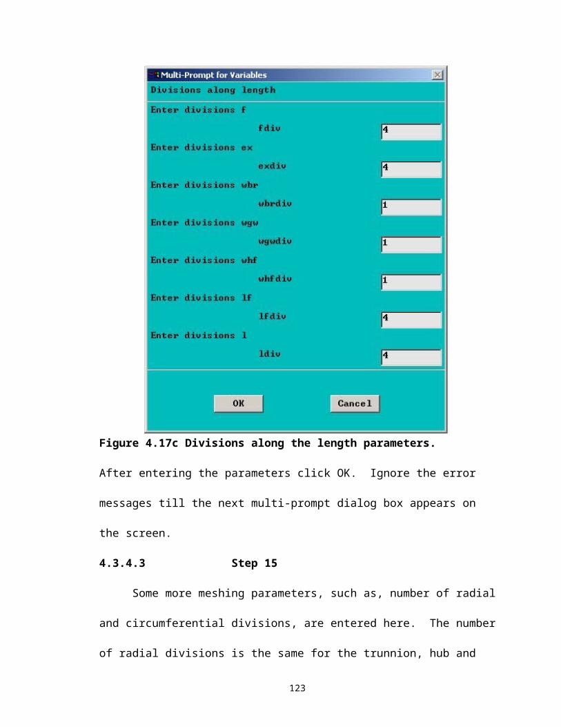
Figure 5.16 Critical parameters plotted against time (full assembly process during AP#2 of the Hillsborough Avenue Bridge).
Table 5.7 Time for each step of AP#2 for the Hillsborough Avenue Bridge.
STEPSTARTIN
GTIME
ENDING
TIMECooling down of the hub (min) 0 3Sliding the hub into the girder (min) 4 753Cooling down the trunnion (min) 754 760Sliding the trunnion into the hub-girder assembly (min) 761 3510
5.8.2.2 Cooling down the hub
The stresses, temperatures and critical crack lengths during this step are plotted
against time in Figure 5.17. A sharp thermal gradient at inner radius of the hub initially
results in high values of hoop stress at the inner radius of the hub. Over time, as the
temperature gradient becomes less steep the hoop stresses fall. The lowest value of
critical crack length during AP#2 is observed this step. The critical crack length (during
138
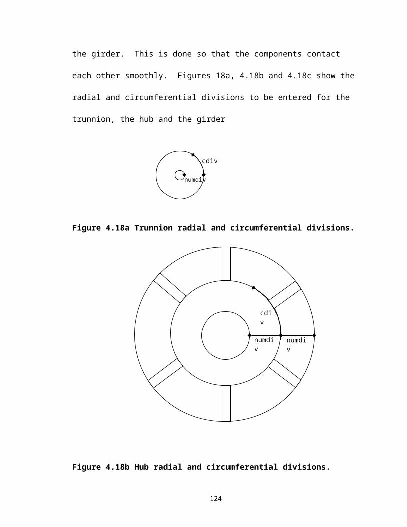
the cooling down of the hub) in AP#1 remains low after reaching its lowest point. Here,
the critical crack length rises after reaching its lowest point. This may explain why
though AP#2 may produce lower values of critical crack length in the assembly, the
probability of crack formation during AP#1 maybe greater (see crack arrest in Section
5.12)
Figure 5.17 Critical parameters plotted against time (cooling down of the hub during AP#2 of the Hillsborough Avenue Bridge).
5.8.2.3 Sliding the hub into the girder
The stresses, temperatures and critical crack lengths during this step are plotted
against time in Figure 5.18. The sharp ‘blip’ in trend of critical crack length is explained
by the extremely low value of tensile hoop stress at that point. The remoteness of the
inner radius of the hub from the hub-girder interface results in low values of hoop stress.
139
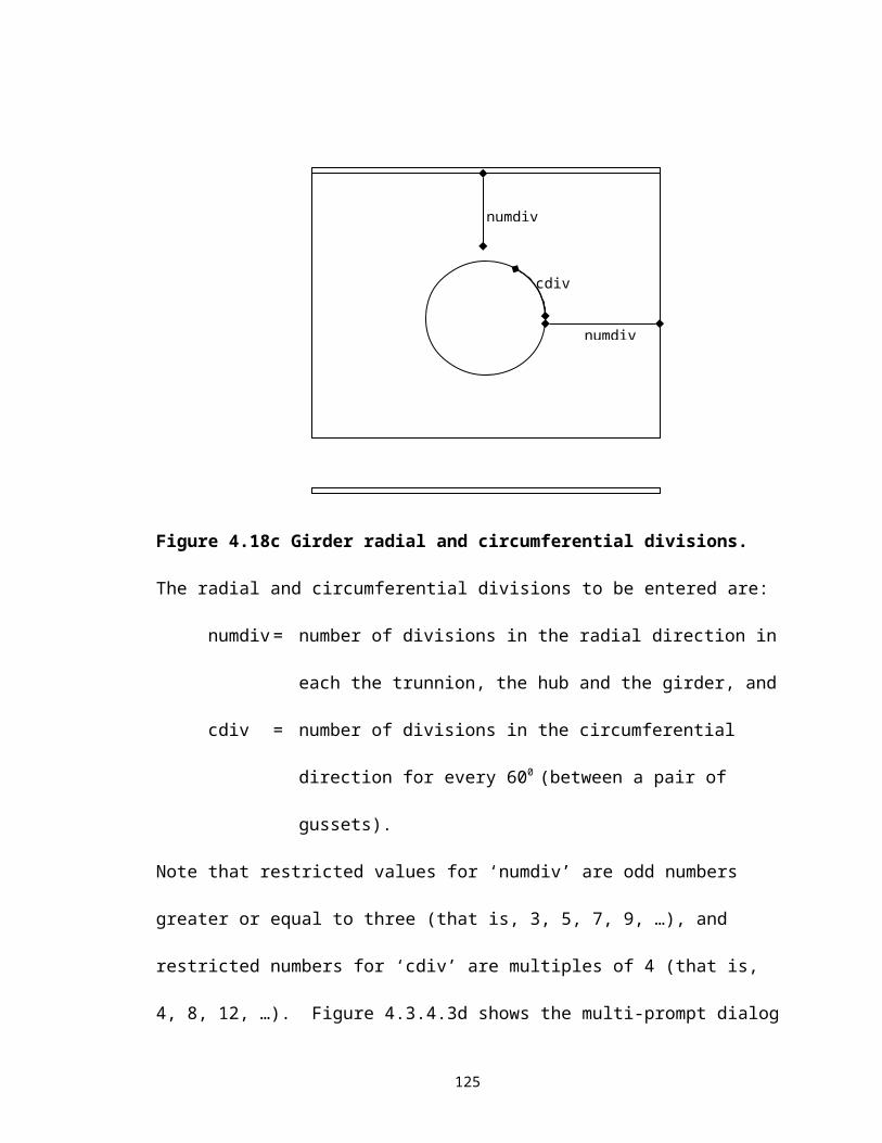
Points where the critical crack length is zero actually indicate compressive hoop stress for
which the critical crack length is not defined.
Figure 5.18 Critical parameters plotted against time (sliding the hub into the girder during AP#2 of the Hillsborough Avenue Bridge).
5.8.2.4 Cooling down of the trunnion
The stresses in the hub are not affected during the cooling down of the trunnion.
5.8.2.5 Sliding the trunnion into the hub-girder
The stresses, temperatures and critical crack lengths during this step are plotted
against time in Figure 5.19. Almost immediately after contact a combination of thermal
stresses due to the sharp thermal gradient and structural stresses due to interference result
in high hoop stresses. Over time, due to the effects of conduction and convection the
temperatures in the assembly converge to about the same temperature. High values of
critical crack length indicate low probability of crack formation during this step.
140
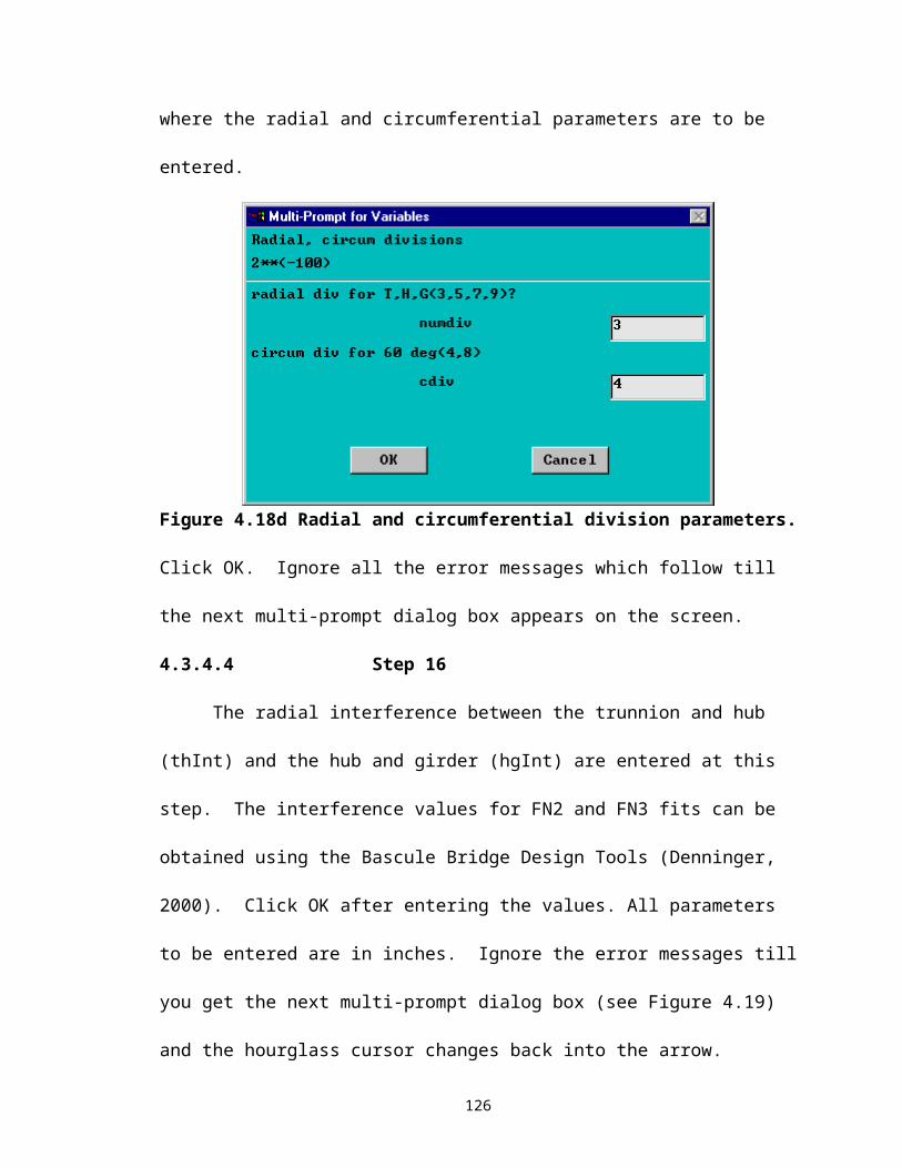
Figure 5.19 Critical parameters plotted against time (sliding the trunnion into the hub-girder during AP#2 of the Hillsborough Avenue Bridge).
5.9 17th Street Causeway
Possible critical points in the assembly are studied using the THGTM. The point
on the inner radius of the hub on the gusset side is found to be the most critical (see
Figure 5.20).
141
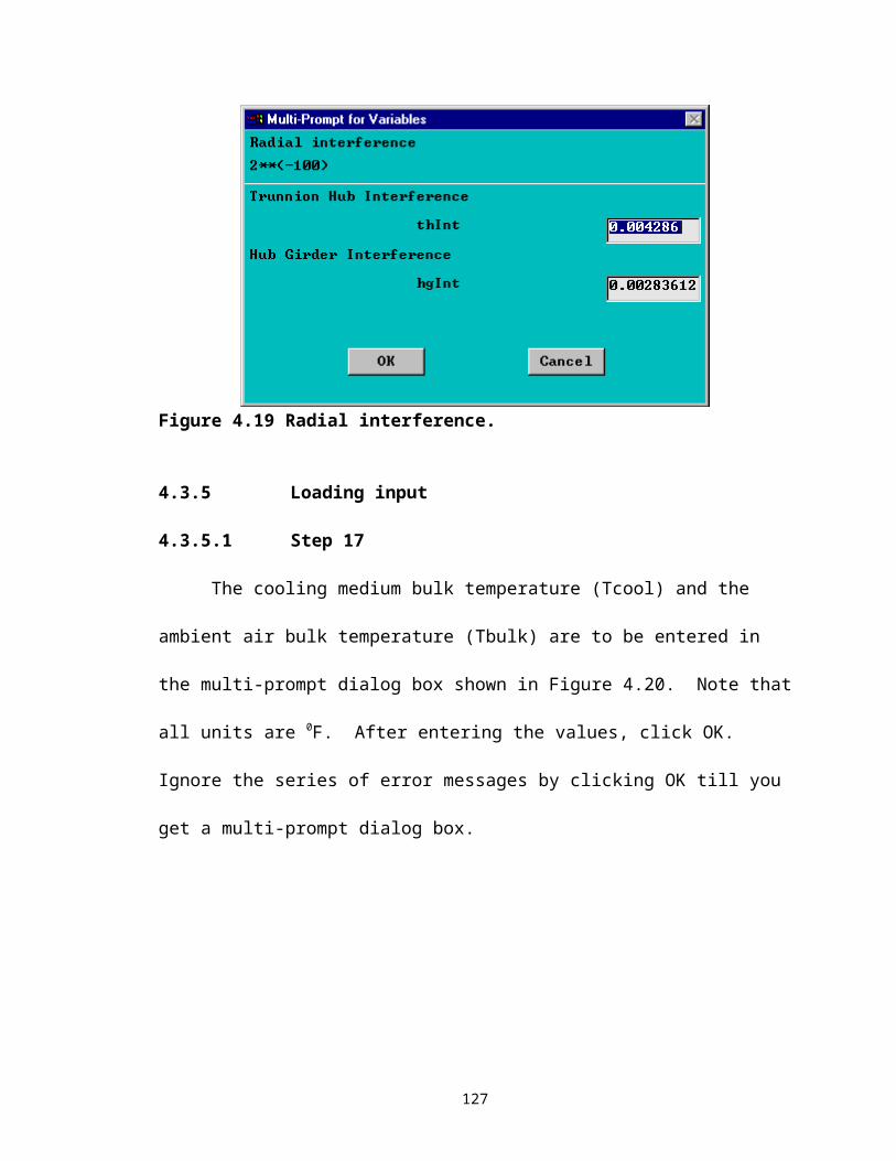
Figure 5.20 Front and side view of the chosen element in the 17th Street Causeway hub.
5.9.1 Assembly procedure 1 (AP#1)
5.9.1.1 Full assembly process
The stresses, temperatures and critical crack lengths of the inner radius of the hub
on the gusset side are plotted against time in Figure 5.21. Time periods for each step of
the assembly process are listed in Table 5.8.
142
Element
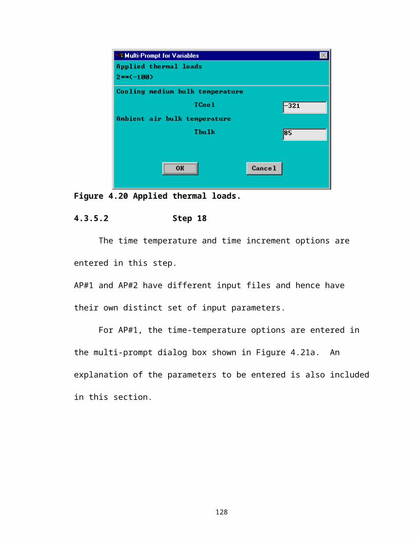
Figure 5.21 Critical parameters plotted against time (full assembly process during AP#1 of 17th Street Causeway Bridge).
Table 5.8 Time for each step of AP#1 for the 17th Street Causeway Bridge.
STEPSTARTIN
GTIME
ENDING
TIMECooling down of the trunnion (min) 0 3Sliding the trunnion into the hub (min) 4 1803Cooling down the trunnion-hub assembly (min) 1803 1805Sliding the trunnion-hub assembly into the girder (min) 1806 2605
5.9.1.2 Cooling down of the trunnion
The stresses in the hub are not affected during the cooling down of the trunnion.
5.9.1.3 Sliding the trunnion into the hub
The hoop stress, the critical crack length and temperature during this step are
plotted against time in Figure 5.22. Thermal and structural stresses due to interference
result in high hoop stresses after contact. As the temperature in the assembly converges
143
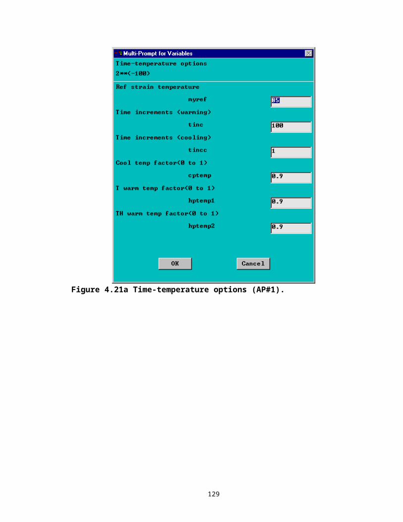
due to the effects of conduction and convection, stresses due to interference become
predominant. High values of critical crack length indicate a low possibility of failure.
Figure 5.22 Critical parameters plotted against time (sliding the trunnion into the hub during AP#1 of 17th Street Causeway Bridge).
5.9.1.4 Cooling down the trunnion-hub assembly
The hoop stress, temperature and the critical crack length for this step are plotted
against time in Figure 5.23. The results from the THGTM indicate that the lowest values
of critical crack length during AP#1 are observed during this step. Initially thermal and
structural stresses reinforce each other and high hoop stresses occur as a result. As the
trunnion-hub assembly nears steady state, the stresses due to interference dominate. An
interesting point to note is that while the critical crack length in the Christa McAuliffe
and Hillsborough assemblies stays low after its lowest point, here it rises steeply after its
lowest point.
144
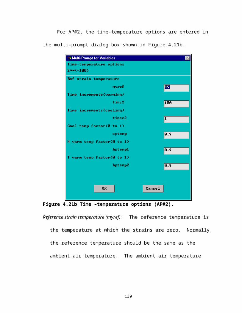
Figure 5.23 Critical parameters plotted against time (cooling down of the trunnion-hub assembly during AP#1 of the 17th Street Causeway Bridge).
5.9.1.5 Sliding the trunnion-hub assembly into the girder
The hoop stress, temperature and the critical crack length during this step are
plotted against time in Figure 5.24. During this step, hoop stresses remain fairly stable
primarily due to the remoteness of the inner radius of the hub from the hub girder
interface. A rise in the temperature due to conduction and convection is accompanied
with a rise in hoop stress. High values of critical crack length indicate a low probability
of crack formation during this step.
145
Figure 5.24 Critical parameters plotted against time (sliding the trunnion-hub assembly into the girder during AP#1 of the 17th Street Causeway Bridge).
5.9.2 Assembly Procedure 2 (AP#2)
5.9.2.1 Full assembly process
The stresses, temperatures and critical crack lengths at the inner radius of the hub
on the gusset side are plotted against time in Figure 5.25.
146
Figure 5.25 Critical parameters plotted against time (full assembly process during AP#2 of the 17th Street Causeway Bridge).
Table 5.9 Time for each step of AP#2 for the 17th Street Causeway Bridge.
STEPSTARTIN
GTIME
ENDING
TIMECooling down of the hub (min) 0 52Sliding the hub into the girder (min) 53 252Cooling down the trunnion (min) 252 256Sliding the trunnion into the hub-girder assembly (min) 257 1456
5.9.2.2 Cooling down of the hub
The stresses, temperatures and critical crack lengths during this step are plotted
against time in Figure 5.26. A sharp thermal gradient at the inner radius of the hub
initially results in high values of hoop stress at the inner radius interface. Over time, as
the temperature gradient becomes less steep, the hoop stresses fall. The lowest value of
147
critical crack length during AP#2 is observed in this step. The critical crack length shows
a distinctly different trend from that the trends observed in other bridges. Here, the
critical crack length starts from a low value and climbs steeply as the temperature in the
assembly falls, once again highlighting the differences between different bridges
Figure 5.26 Critical parameters plotted against time (cooling down of the hub during AP#2 of 17th Street Causeway Bridge).
5.9.2.3 Sliding the hub into the girder
The stresses, temperatures and critical crack lengths during this step are plotted
against time in Figure 5.27. The relatively low values of compressive hoop stress are
explained by the remoteness of the inner radius of the hub from the hub-girder interface.
The critical crack length is not defined for compressive hoop stress and hence is plotted
as zero at these points.
148
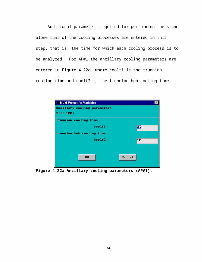
Figure 5.27 Critical parameters plotted against time (sliding the hub into the girder during AP#2 of the 17th Street Causeway Bridge).
5.9.2.4 Cooling down of the trunnion
The stresses in the hub are not affected during the cooling down of the trunnion.
5.9.2.5 Sliding the trunnion into the hub-girder assembly
The stresses, temperatures and critical crack lengths during this step are plotted
against time in Figure 5.28. The behavior of hoop stress is somewhat different from that
of other bridges. In the other two bridge assemblies, high initial hoop stress caused due a
thermal gradient is followed by a fall in hoop stress as the assembly approaches steady
state. Here the hoop stress rises and then falls before rising again. However the
magnitude of this variation is is small. High values of critical crack length discount the
probability of crack formation during this step.
149
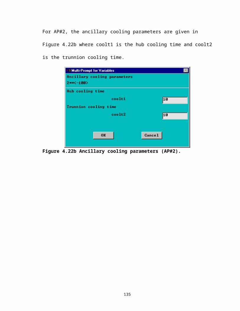
Figure 5.28 Critical parameters plotted against time (sliding the trunnion into the hub-girder assembly during AP#2 of the 17th Street Causeway Bridge).
5.10 Comparison
A comparison, for all of the bridges presented in the beginning of this chapter, of
the highest hoop stress and minimum crack length is presented in Table 5.10.
Table 5.10 Minimum critical crack length and maximum hoop stress for different assembly procedures and different bridges.
BRIDGE PARAMETER AP#1 AP#2Christa
McAuliffeMinimum Critical Crack Length (in) 0.2101 0.2672Maximum Hoop Stress (ksi) 28.750 33.424
HillsboroughAvenue
Minimum Critical Crack Length (in) 0.5577 0.1898Maximum Hoop Stress (ksi) 29.129 32.576
17th Street Causeway
Minimum Critical Crack Length (in) 0.6420 1.0550Maximum Hoop stress (ksi) 15.515 17.124
An examination of the results reveal significant differences in the behavior of
each bridge. In some bridges, a lower critical crack length is found to occur during AP#1
150
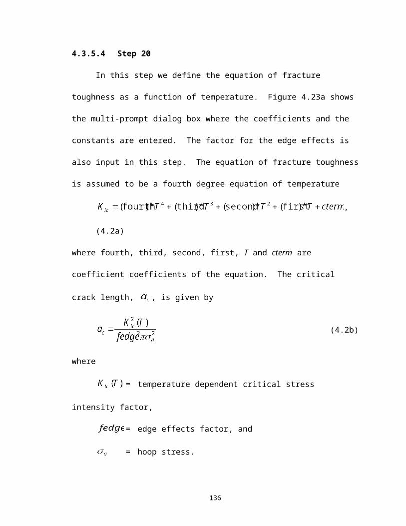
(that is, Christa McAuliffe and 17th Street Causeway) while in others (that is,
Hillsborough Avenue) the opposite is true. In addition, a slightly lower value of critical
crack length during AP#1 versus AP#2 of Christa McAuliffe Bridge is observed. A
simple comparison of critical crack lengths, however is not sufficient to conclude the
superiority of one assembly procedure over another for each bridge. A phenomenon
called crack arrest described in the next section can explain how in some cases crack
formation can be arrested in spite of low values of critical crack length during the
assembly process.
The maximum hoop stress is less than the ultimate tensile strength (36 ksi) in all
the bridge assemblies indicating that they will not fail due to yielding.
5.11 Crack arrest
Crack arrest is the reverse of crack initiation. Small cracks present in the
assembly grow fast after exceeding the fracture toughness of the material. Crack arrest
may prevent these cracks from growing catastrophically. The condition required for this
phenomenon to occur is evaluated by the parameter , which is the critical crack arrest
factor. Crack growth is arrested once
(5.3a)
In Equation (5.3a), is determined by the equation (Kanninen, Melvin and Popelar,
1985)
(5.3b)
where
= calculated parameter based on the hoop stress and the crack
length ,
151
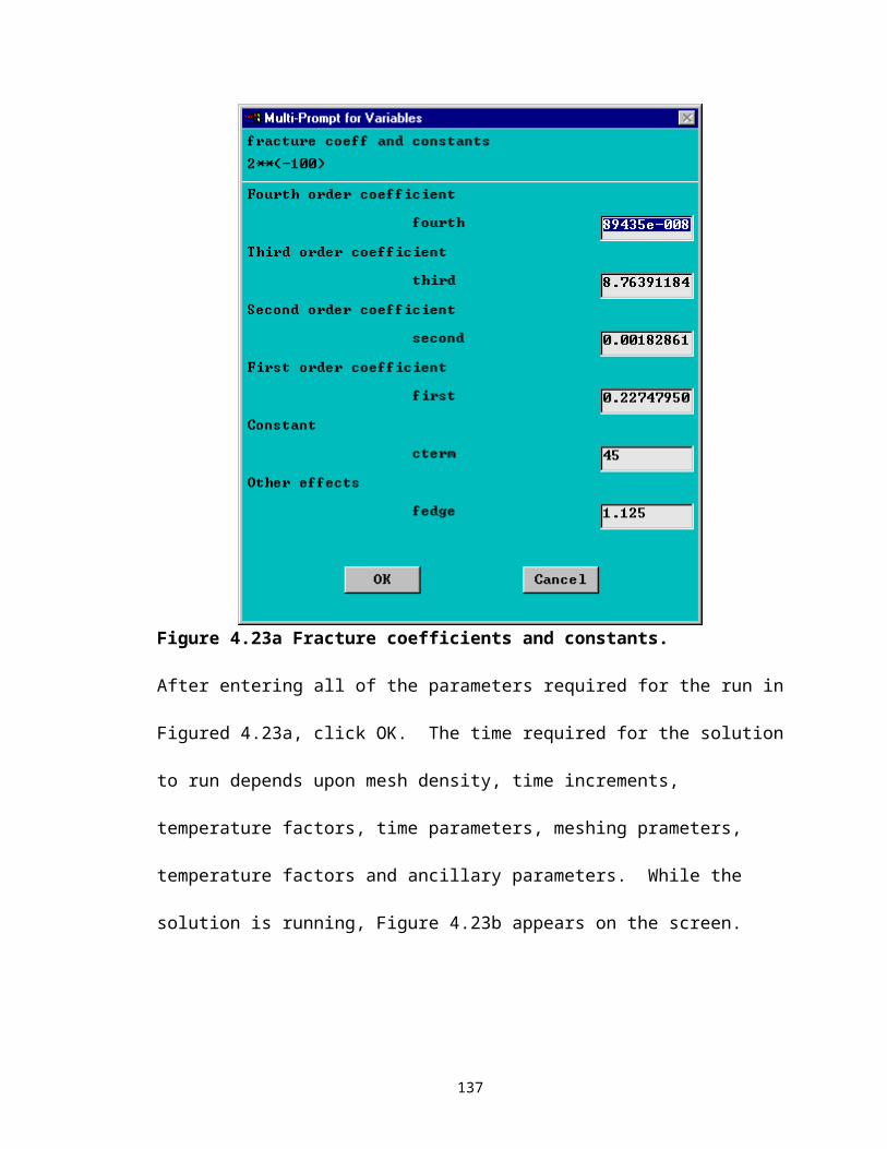
= hoop stress, and
= crack length.
The variation of with temperature is shown in Figure 5.29a for A508 steel. It
follows a trend similar to that of .
Figure 5.29a and against temperature for A508 steel (Kanninen et al. 1985).
The crack length at which crack arrest will occur, , is given by the Equation (5.3c).
(5.3c)
This phenomenon is of relevance to this study as sharp thermal gradients may
result in low values of the fracture toughness, which may not necessarily lead to
catastrophic crack growth. To illustrate this phenomenon, let us take the case of the
Hillsborough Avenue Bridge. Figures 5.29b and 5.29c show the critical parameters
during the cooling down of the trunnion-hub (AP#1) and cooling down of the hub
(AP#2), respectively. The lowest value of critical crack length is lower during AP#2
152
(0.1898 in) than during AP#1 (0.5577 in). However, the critical crack length during
AP#1 remains low for a considerable period of time, whereas in AP#2 it shows a sharp
upward trend after its lowest point. From Figure 5.11a it is clear that the and
follow similar trends. In AP#2 crack growth initiated by may be arrested as
with fall in hoop stress. In AP#1, the persistent low values of critical crack
length indicate that the values will also be low, thereby preventing crack arrest.
The possibility of crack arrest is greater when thermal stresses alone are present
as they are transient and change rapidly. However, when a combination of both thermal
and interference stresses are present, the possibility of crack arrest occurring is greatly
reduced. Hence, crack arrest is more likely to occur during AP#2 than during AP#1.
Figure 5.29b Critical parameters plotted against time (cooling down of the trunnion-hub assembly during AP#1 of the Hillsborough Avenue Bridge).
153
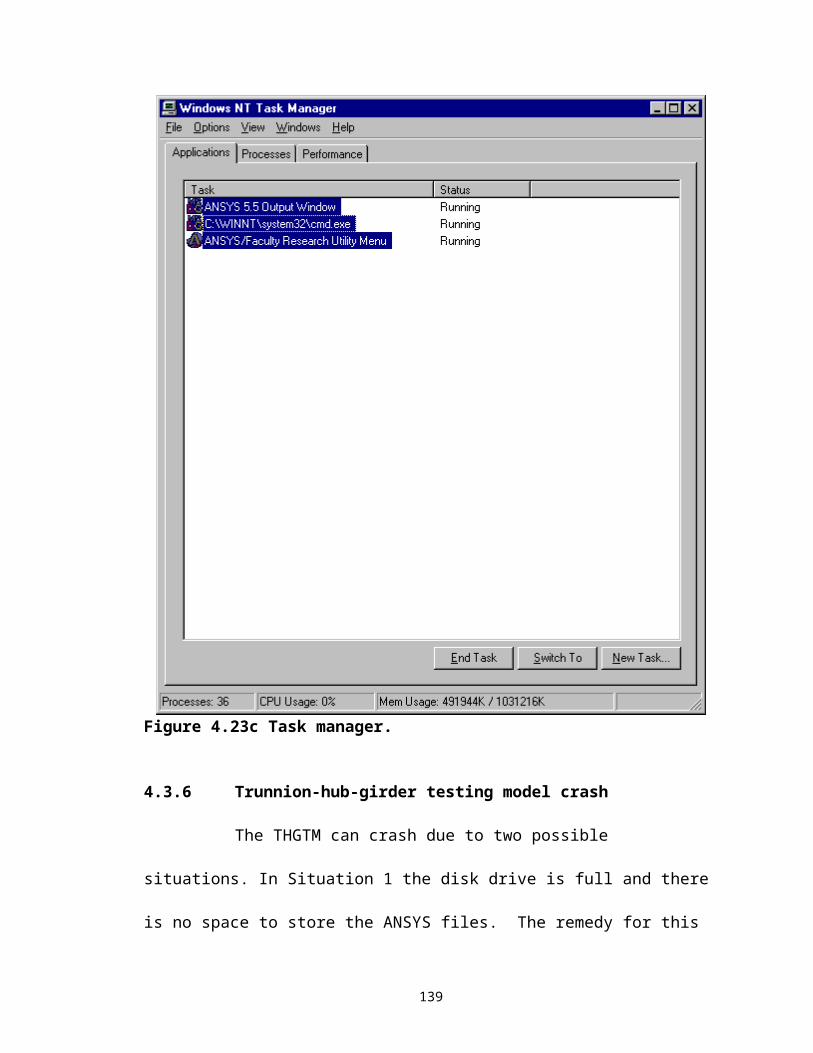
Figure 5.29c Critical parameters plotted against time (cooling down of the hub during AP#2 of the Hillsborough Avenue Bridge).
5.12 Possibility of failure during the insertion process and gap conduction
The most critical steps during the assembly process are determined to be the
cooling processes. However, the possibility of failure during the warming up process
also needs to be explored.
In this study male parts of the assembly are inserted into female parts as soon as
the interference between them is breached. Hence, there is no gap conduction between
the two parts. This is done principally because this models the worst case from the
perspective of failure during the insertion of one part of the assembly into another. The
reason for this explained next.
Thermal stresses are caused due to thermal gradients. Hence, the sharper thermal
gradient (between the outer radius of the male part and inner radius of the female part)
154
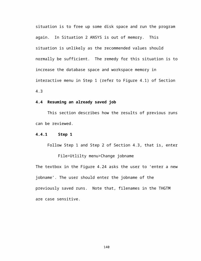
during the insertion of one part the assembly into another the greater are the thermal
stresses. Cooling down a part of the assembly till the interference breached results in a
sharper thermal gradient between parts of the assembly than cooling the male part down
until there is gap between the two parts and then subsequently warming parts of the
assembly by a combination of convection and gap conduction up to the point of contact.
This is so primarily because gap conduction results in faster heat flux and lowers the
temperature difference between the outer radius of the male part and inner radius of the
female part. Hence, the insertion of the male part into the female part as soon as
interference is breached is the worst case from the perspective of failure.
By modeling the worst case, we know which assemblies have a greater proneness
to failure during the insertion process. For example, during AP#1 of the Hillsborough
Avenue Bridge, low values of critical crack length are noticed during AP#1. Hence, it is
advisable that during assembly we cool down parts of the assembly until there is large
gap between them during assembly.
5.13 Conclusions and recommendations
Our hypothesis at the beginning of this study was that AP#2 resolves the
problems associated with AP#1. The results broadly agree with this hypothesis.
However each bridge is different and needs to be analyzed separately. There can be
possible situations where AP#1 may turn out to be a better process. One common
problem associated with both assembly processes studied is thermal shock. In AP#2, the
sharp thermal gradient sometimes leads to very low values of critical crack length. In
AP#1, a combination of high thermal and interference stresses results in possibility of
crack formation. A lower thermal gradient can improve both the assembly processes.
155
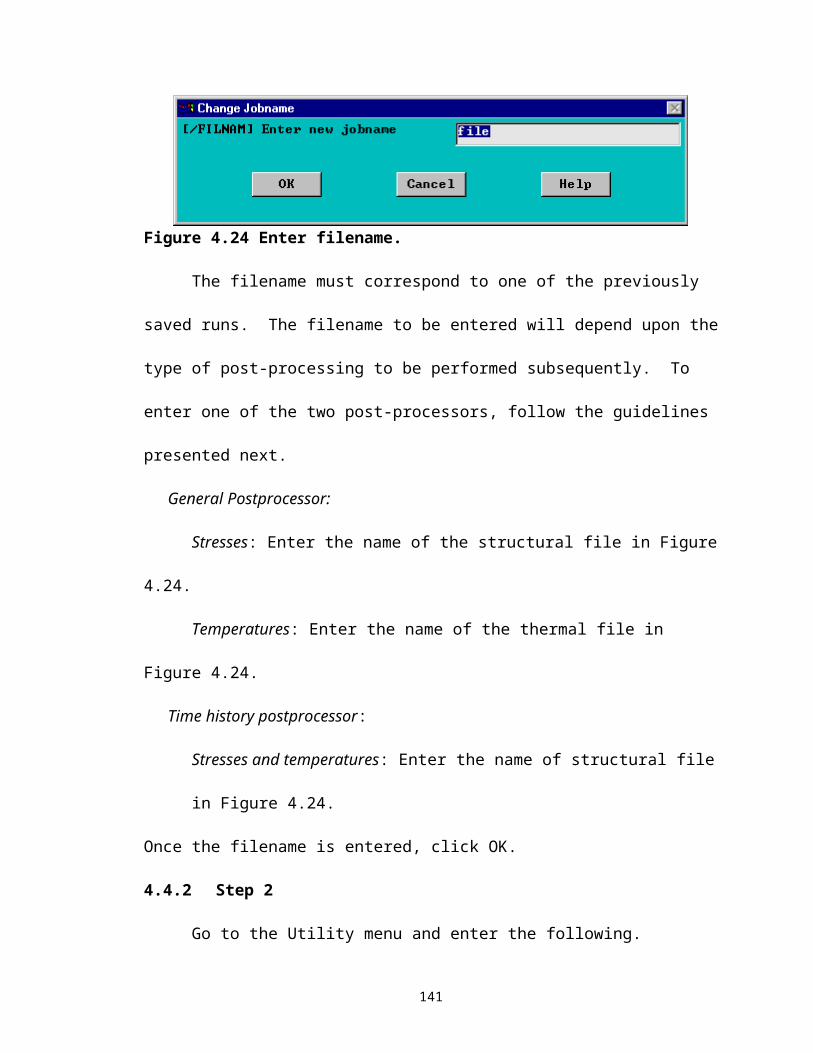
Some recommendations during assembly are:
1. Before choosing the assembly procedure for a bridge, the THGTM
should be run and the following questions need to be answered:
a. What are the values of the critical crack length during the critical steps in the
assembly process? During which process does a lower value of critical crack
length exist?
b. How long do the values of critical crack length remain low? Are there
indications of crack arrest?
c. What are the highest values of hoop stress and when do they occur?
d. What are values of critical crack length and hoop stress during the two
warming up processes?
2. Avoid sharp thermal gradients to create lower thermal stresses. It is advisable
to perform a part of the cooling process in a medium with a lower convective heat
transfer coefficient and boiling point than liquid nitrogen before dipping it in
liquid nitrogen. For example, immersion in liquid nitrogen could be preceded by
immersion in a mixture of dry ice and alcohol.
3. In general, it is better cool parts of the assembly until there is a reasonable gap
between the male and the female part before insertion. This is particularly true if
the THGTM indicates low values of critical crack length during the process.
156
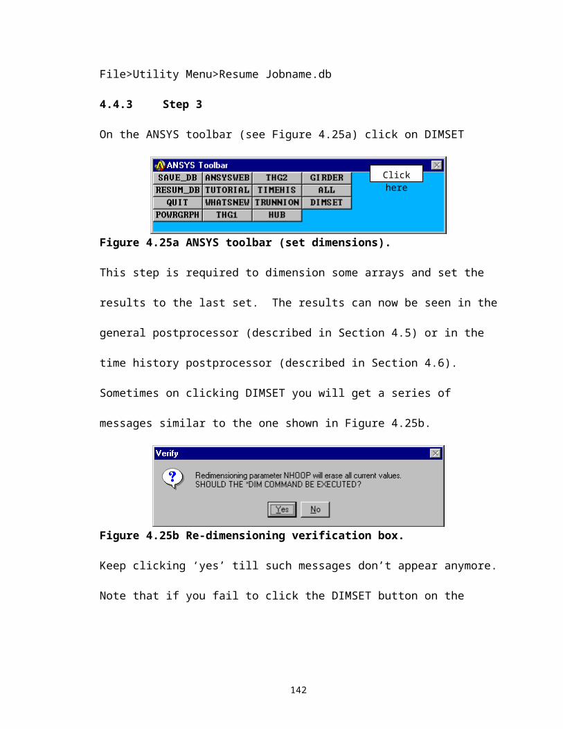
REFERENCES
Brentari E. G. and Smith R. V. “Nucleate and Film Pool Boiling Design Considerations for 02, N2, H2 and He.” International Advances in Cryogenic Engineering 10b (1964) :325-341
Denninger, Michael T. “Design Tools for Trunnion-Hub Assemblies for Bascule Bridges.” Masters Thesis, University of South Florida, August 2000.
Kanninen, Melvin F, and Carl H Popelar. Advanced Fracture Mechanics, Oxford Engineering Science Series. New York: Oxford University Press, 1985.
Logan, Daryl L. A First Course in Finite Element Method. 2 ed, PWS-KENT Series in Engineering. Boston: PWS-KENT Publishing Company, 1992.
Noda, Naotake. “Transient Thermoelastic Contact Problem in a Cylinder with a Position-Dependent Heat Transfer Coefficient.” Journal of Thermal Stresses 10 (1987): 57-69.
Noda, Naotake. “Transient Thermoelastic Contact Stresses in a Short-Length Circular Cylinder.” Journal of Thermal Stresses 8 (1985): 413-424.
Noda, Naotake. “Transient Theromelastic Contact Problem in a Long Circular Cylinder.” Journal of Thermal Stresses 7 (1984): 135-147.
Oliviera, R, and X R Wu. “Stress Intensity Factors for Axial Cylinders Subjected to Thermal Shock.” Engineering Fracture Mechanics 27, (1987): 185-197.
Ootao, Y, T Akai, and Y Tanikawa. “Three-Dimensional Transient Thermal Stress Analysis of a Non-Homegenous Hollow Circular Cylinder Due to a Moving Heat Source in the Axial Direction.” Journal of Thermal Stresses 18 (1995): 497-512.
Ozisik, M Necati. Basic Heat Transfer. New York: McGraw-Hill Book Company, 1977.
Pourmohamadian, H, and M Sabbaghian. “Transient and Residual Thermal Stresses in a Solid Cylinder with Temperature Dependent Material Properties.” ASME Pressure Vessel and Piping 98-8 (1987) 33-41.
Reed, Richard P. Materials at Low Temperatures. Metals Park: American Society for Metals, 1983.
157
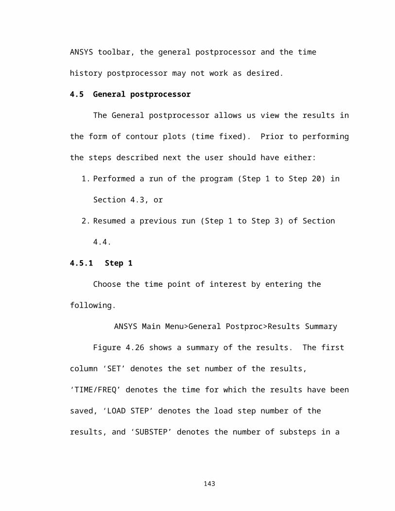
Thomas, J R Jr., J P Sing, H Tawil, L Powers, and D P H Hasselman. “Thermal Stresses in a Long Circular Cylinder Subjected to Sudden Cooling During Transient Convection Heating.” Journal of Thermal Stresses 8 (1985): 249-260.
Ugural, Ansel C, and Saul K Fenster. Advanced Strength and Applied Elasticity. 3 ed. New Jersey: Prentice-Hall, 1995.
158
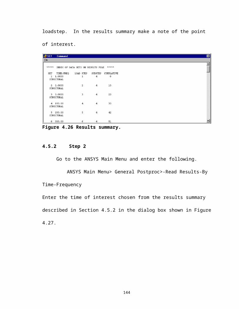
.
159