Chapter10 HiddenMarkovModels - rileylab.orgrileylab.org/wp-content/uploads/2016/08/IntroBio... · Chapter10 HiddenMarkovModels TheMarkovprocessformsthebasisofmanyimportantmodelsinbioinfor-matics,

Chapter 10

Hidden Markov Models

The Markov process forms the basis of many important models in bioinfor-matics, including Markov Models and Hidden Markov Models (HMMs) forsequence alignments, protein folding, protein-DNA binding, and phylogenetictrees. For sequence alignments, the BLOSUM, PAM, and other alignmentmatrices are constructed on the basis of a Markov process. With phyloge-netic trees, it is possible to estimate evolutionary distances between severalsequences and to visualize them with a tree. Lastly, Hidden Markov Modelscan learn, for example, the conserved amino acid characteristics of differ-ent protein families in order to model protein homology and predict proteinfamily membership.

In this chapter, we will learn about the probability transition matrixand the role it plays in a Markov process to construct specific sequences.In addition, various models for building phylogenetic trees are explained interms of the rate matrix and the probability transition matrix. Lastly, thebasic ideas of the Hidden Markov Model are briefly explained and illustratedby examples1.

10.1 Markov Process

A stochastic process is a sequence of events in which the outcome at anystage depends on some probability. A Markov process is a type of stochasticprocess with the following properties:

1This chapter is somewhat more technical in its notation (e.g. conditional probability).However, this is necessary to understand Markov processes.

257

258 CHAPTER 10. HIDDEN MARKOV MODELS

1. The number of possible outcomes or states is finite.2. The outcome at any stage depends only on the outcome of the previous

stage.3. The probabilities are constant over time.

Property number 2 is often referred to as memorylessness. In a Markovprocess, no memory of previous states is required to predict the next statein the process - only the current state determines the next state. We willintroduce Markov processes with a couple of simple examples. A Markovmodel is a statistical model in which the system being modeled is assumedto be a Markov process.

10.2 Random sampling

Probabilistic Markov models used to predict and classify biological sequencesmake it possible to draw a random sample from a parameterized population.Fundamentally, these models sample from one or more probability distribu-tion. Recall from Chapter 3 that a discrete distribution is a set of discretevalues with certain probabilities that add up to one. The following two basicexamples illustrate this point:

Example 1: Tossing a coin. When tossed high into the air, a fair coinX comes up Heads and Tails each with probability 1/2. Thus, we define theprobabilities of each outcome with P (X = H) = 0.5 and P (X = T ) = 0.5 -where the letters H and T corresponding to the outcomes Heads and Tails,respectively. No matter how many outcomes, with such a random variablethere always exists an outcome population as well as a sampling schemewhich can properly model all the possible sequences of outcomes - which arecalled observed events (e.g. Press, et al., 1992).

To model the event of repeatedly tossing a coin into the air, we can use thesample() command to define the probabilities of each outcome and specifythe number of tosses. The noquote() function just removes all quotes fromthe output.> noquote(sample(c("H","T"),30,rep=TRUE,prob=c(0.5,0.5)))[1] T H H H H H H H T T H H H H H H T T T T H T H H T T H T H T

Thus, the sampled outcomes of Heads and Tails correspond to the eventof a Markov process of repeatedly tossing a fair coin. In the above exam-ple, the sample() function randomly draws thirty times one of the outcomes

10.3. PROBABILITY TRANSITION MATRIX 259

c("H","T") with replacement (rep=TRUE) and equal probabilities (prob=c(0.5,0.5)).The event that we observed was the set of outcomes T H H H H H H H T TH H H H H H T T T T H T H H T T H T H T

Example 2: Generating a sequence of nucleotides. Another ex-ample is that of a random variable X which has (letters corresponding to)nucleotides as its outcomes. The outcomes are X = A, X = C, X = G,and X = T . For example, let us define these outcomes for a specific familyof DNA sequences with probabilities P (X = A) = 0.1, P (X = G) = 0.4,P (X = C) = 0.4, and P (X = T ) = 0.1. A DNA sequence that is sampledfrom this discrete probability distribution represents a sequence event thatis modeled by the Markov process. In R, let us sample() from this Markovprocess to produce a 30 base pair sequence (event):

> noquote(sample(c("A","G","C","T"),30,rep=TRUE,prob=c(0.1,0.4,0.4,0.1)))[1] G C C C C C A G A T C G G G G T G G G C G G G G G C C T C C

Of course, if you do this again, then the resulting sequence will differ dueto the random nature of its generation.

10.3 Probability transition matrix

In order to build a Markov model that produces specific sequences, we willconsider a certain type of random variable. In particular, we will consider asequence {X1, X2, · · · } with values from a certain state space E. The latteris simply a set containing the possible values or states of a process. If,for instance, Xn = i, then the process is in state i at time n. Similarly,the expression P (X1 = i) denotes the probability that the process is instate i at time point 1. The event that the process changes its state from ito j (transition) between time point one and two corresponds to the event(X2 = j|X1 = i), where the bar means "given that". The probability forthis event to happen is denoted by P (X2 = j|X1 = i). And in general, theprobability of the transition from i to j between time point n and n + 1 isgiven by P (Xn+1 = j|Xn = i). Lastly, these probabilities can be collected ina probability transition matrix P with elements

pij = P (Xn+1 = j|Xn = i).


We will assume that the transition probabilities are the same for all timepoints so that there is no time index needed on the left hand side. Giventhat the process Xn is in a certain state, the corresponding row of the transi-tion matrix contains the distribution of Xn+1, implying that the sum of theprobabilities over all possible states equals one. The probability transitionmatrix contains a (conditional) discrete probability distribution on each ofits rows. For a Markov process it holds that the state at time point n+ 1 de-pends upon the state at time point n, but not on states at earlier time points.

Example 1: The probability transition matrix. Suppose Xn hastwo states: Y for a pyrimidine and R for a purine. A sequence can nowbe generated, as follows. If Xn = Y , then we throw with a fair die: Ifthe outcome is lower than or equal to 5, then Xn+1 = Y and, otherwise,Xn+1 = R. If Xn = R, then we throw with a fair coin: If the outcome equalsTail, then Xn+1 = Y , and otherwise Xn+1 = R. For this process the two bytwo probability transition matrix equals

from

toY R

Y pY Y pY RR pRY pRR

where pRY is the probability that the process changes from R to Y. Thistransition matrix can also be written as

P =

[pY Y pY RpRY pRR

]=

[P (X1 = Y |X0 = Y ) P (X1 = R|X0 = Y )P (X1 = Y |X0 = R) P (X1 = R|X0 = R)

]=

[56

16

12

12

].

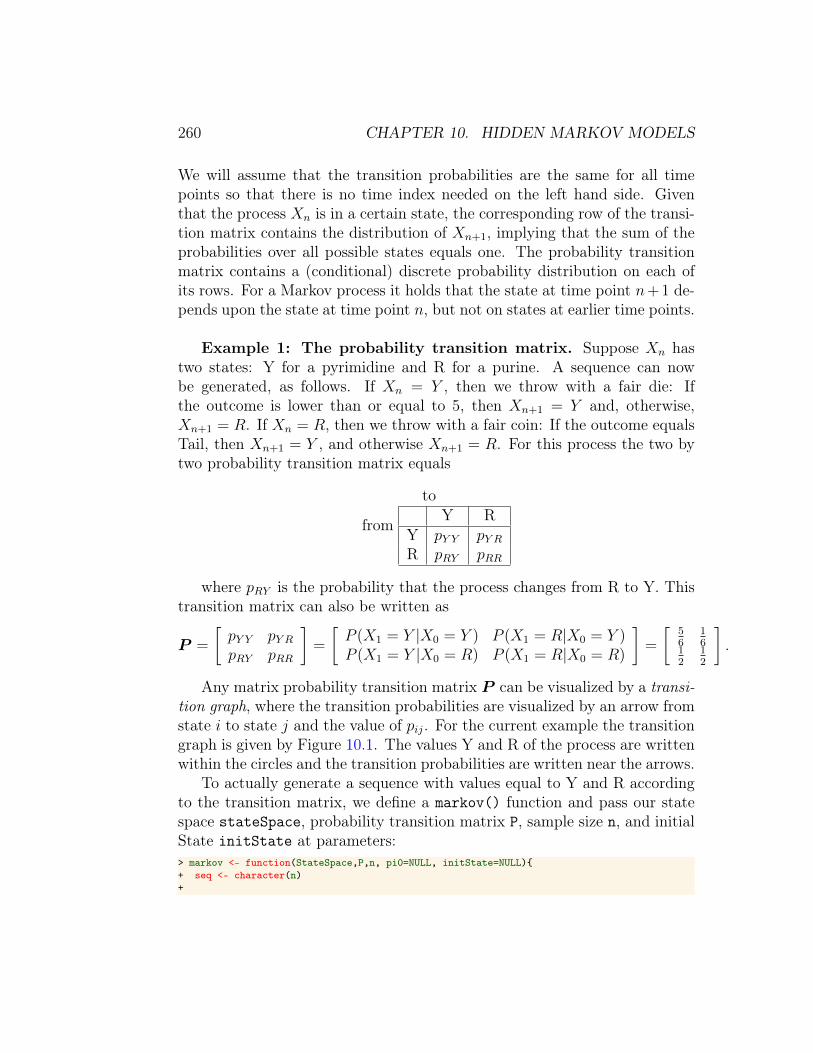
Any matrix probability transition matrix P can be visualized by a transi-tion graph, where the transition probabilities are visualized by an arrow fromstate i to state j and the value of pij. For the current example the transitiongraph is given by Figure 10.1. The values Y and R of the process are writtenwithin the circles and the transition probabilities are written near the arrows.

To actually generate a sequence with values equal to Y and R accordingto the transition matrix, we define a markov() function and pass our statespace stateSpace, probability transition matrix P, sample size n, and initialState initState at parameters:> markov <- function(StateSpace,P,n, pi0=NULL, initState=NULL){+ seq <- character(n)+


5/6

1/6

1/2

1/2

Y R

Figure 10.1: Graph of the probability transition matrix

+ if (is.null(pi0)) {+ seq[1] <- initState+ }+ else {+ seq[1] <- sample(StateSpace, 1, replace=TRUE, pi0)+ }++ for(k in 1:(n-1)) {+ seq[k+1] <- sample(StateSpace, 1, replace=TRUE, P[seq[k],])+ }++ return(seq)+ }>> P <- matrix(c(1/6,5/6,0.5,0.5), 2, 2, byrow=TRUE)> rownames(P) <- colnames(P) <- stateSpace <- c("Y","R")> P

Y RY 0.1666667 0.8333333R 0.5000000 0.5000000> noquote(markov(stateSpace,P,30,initState="Y"))[1] Y Y R Y R Y R R Y Y R Y R R R Y Y R Y R Y R R R Y R Y R Y R

In the function markov(), the actual sampling is performed by the sample()function. Note that we must pass in either an initial State initState or aninitial probability distribution Pi0 for the initial state. Then we sample oneelement at a time from the set containing Y and R according to the prob-abilities in row seq[k] of the matrix P. This makes the probabilities of thestates dependent on the corresponding row of the transition matrix. We con-veniently use the fact that R adds an element to the sequence; we do nothave to declare its length beforehand. In this example, the sequence has afixed start at State Y and thereafter the first row in the probability transitionmatrix. Note that without the return command the function does not return


any output.

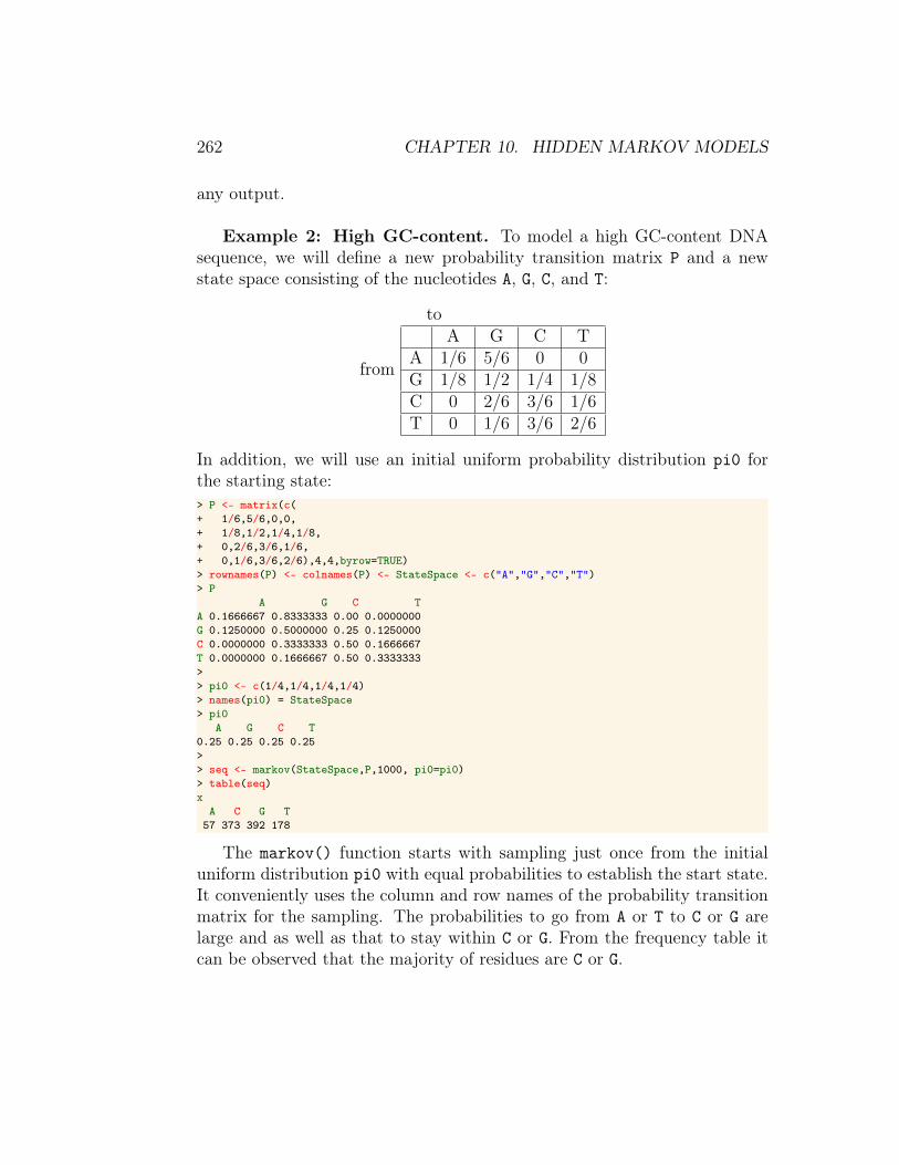
Example 2: High GC-content. To model a high GC-content DNAsequence, we will define a new probability transition matrix P and a newstate space consisting of the nucleotides A, G, C, and T:

from

toA G C T

A 1/6 5/6 0 0G 1/8 1/2 1/4 1/8C 0 2/6 3/6 1/6T 0 1/6 3/6 2/6

In addition, we will use an initial uniform probability distribution pi0 forthe starting state:> P <- matrix(c(+ 1/6,5/6,0,0,+ 1/8,1/2,1/4,1/8,+ 0,2/6,3/6,1/6,+ 0,1/6,3/6,2/6),4,4,byrow=TRUE)> rownames(P) <- colnames(P) <- StateSpace <- c("A","G","C","T")> P

A G C TA 0.1666667 0.8333333 0.00 0.0000000G 0.1250000 0.5000000 0.25 0.1250000C 0.0000000 0.3333333 0.50 0.1666667T 0.0000000 0.1666667 0.50 0.3333333>> pi0 <- c(1/4,1/4,1/4,1/4)> names(pi0) = StateSpace> pi0

A G C T0.25 0.25 0.25 0.25>> seq <- markov(StateSpace,P,1000, pi0=pi0)> table(seq)x

A C G T57 373 392 178

The markov() function starts with sampling just once from the initialuniform distribution pi0 with equal probabilities to establish the start state.It conveniently uses the column and row names of the probability transitionmatrix for the sampling. The probabilities to go from A or T to C or G arelarge and as well as that to stay within C or G. From the frequency table itcan be observed that the majority of residues are C or G.


Example 3: High phenylalanine content. In this example we wishto construct DNA sequences that translate into amino acid sequences withhigh phenylalanine (F) content. Recall that phenylalanine (F) is coded bythe triplet codon TTT or TTC. Therefore, we will construct a DNA Markovmodel that emits Ts with high probability:

from

toA G C T

A 0.01 0.01 0.01 0.97G 0.01 0.01 0.01 0.97C 0.01 0.01 0.01 0.97T 0.01 0.28 0.01 0.70

We use the function getTrans() of the seqinr package to translate thegenerated nucleotide triplets into amino acids.> P <- matrix(c(.01,.01,.01,.97,+ .01,.01,.01,.97,+ .01,.01,.01,.97,+ .01,.28,.01,0.70),4,4,byrow=T)> rownames(P) <- colnames(P) <- StateSpace <- c("A","G","C","T")> P

A G C TA 0.01 0.01 0.01 0.97G 0.01 0.01 0.01 0.97C 0.01 0.01 0.01 0.97T 0.01 0.28 0.01 0.70>> pi0 <- c(1/4,1/4,1/4,1/4)> names(pi0) = StateSpace> pi0

A G C T0.25 0.25 0.25 0.25>> seq <- markov(StateSpace,P,30000, pi0=pi0)> table(getTrans(seq))

* A C D E F G H I L M N R S T V27 22 2053 19 1 3835 23 1 61 1593 33 1 1 77 1 2161W Y

17 74

From the table it is clear that the phenylalanine (F) frequency is thelargest among all the amino acids in the generated, very long amino acidsequence.

Example 4: Generating the probability transition matrix. Toillustrate estimation of the probability transition matrix we proceed with thesequence seq produced by the previous example.


> nr <- count(tolower(seq),2)> nr

aa ac ag at ca cc cg ct ga gc gg gt ta3 3 2 283 1 2 2 283 76 60 74 6283 211

tc tg tt223 6414 16079

> A <- matrix(NA,4,4)> A[1,1] <- nr["aa"]; A[1,2]<-nr["ag"]; A[1,3]<-nr["ac"]; A[1,4]<-nr["at"]> A[2,1] <- nr["ga"]; A[2,2]<-nr["gg"]; A[2,3]<-nr["gc"]; A[2,4]<-nr["gt"]> A[3,1] <- nr["ca"]; A[3,2]<-nr["cg"]; A[3,3]<-nr["cc"]; A[3,4]<-nr["ct"]> A[4,1] <- nr["ta"]; A[4,2]<-nr["tg"]; A[4,3]<-nr["tc"]; A[4,4]<-nr["tt"]> rowsumA <- apply(A, 1, sum)> Phat <- sweep(A, 1, rowsumA, FUN="/")> rownames(Phat) <- colnames(Phat) <- c("a","g","c","t")> round(Phat,3)

a g c ta 0.010 0.007 0.010 0.973g 0.012 0.011 0.009 0.968c 0.003 0.007 0.007 0.983t 0.009 0.280 0.010 0.701

The number of transitions are counted and divided by the row totals.The estimated transition probabilities are quite close to the true transitionprobabilities. The zero transition probabilities are exactly equal to the truthbecause these do not occur. This estimation procedure can also easily beapplied to amino acid sequences.

10.4 Properties of the transition matrixIn the previous examples, the sequence was started at a certain state. Often,however, only the probabilities of the initial states are available. That is,we have a vector π0 with initial probabilities π10 = P (X0 = 1) and π20 =P (X0 = 2). Furthermore, if the transition matrix is defined as

P =

[p11 p12

p21 p22

]=

[P (X1 = 1|X0 = 1) P (X1 = 2|X0 = 1)P (X1 = 1|X0 = 2) P (X1 = 2|X0 = 2)

],

then the probability that the process is in State 1 at time point 1 can bewritten as

P (X1 = 1) = π10p11 + π20p21 = πT0 p1, (10.1)

where p1 is the first column of P , see Section 10.8. Note that the lastequality holds by definition of matrix multiplication. In a similar manner,it can be shown that P (X1 = 2) = πT0 p2, where p2 is column 2 of the

10.4. PROPERTIES OF THE TRANSITION MATRIX 265

transition matrix P = (p1,p2). It can be concluded that πT0P = πT1 , whereπT1 = (P (X1 = 1), P (X1 = 2)); the probability at time point 1 that theprocess is in State 1, State 2, respectively. This holds in general for all timepoints n, that is

πTnP = πTn+1. (10.2)

Thus to obtain the probabilities of the states at time point n+ 1, we cansimply use matrix multiplication2.

Example 1: Matrix multiplication to compute probabilities. Sup-pose the following initial distribution and probability matrix

π0 =[

23

13

],P =

[56

16

12

12

],

for State 1 and 2, respectively. Then P (X1 = 1) and P (X1 = 2) collected inπT1 = (P (X1 = 1), P (X1 = 2)) can be computed as follows.

πT1 = πT0P =[

23

13

] [ 56

16

12

12

]=[

23· 5

6+ 1

3· 1

223· 1

6+ 1

3· 1

2

]=[

1318

518

]Using R its operator %*% for matrix multiplication, the product πT0P can

be computed as follows.> P <- matrix(c(5/6,1/6,0.5,0.5),2,2,byrow=T)> pi0 <- c(2/3,1/3)> pi0 %*% P

[,1] [,2][1,] 0.7222222 0.2777778

Yet, another important property of the probability transition matrix dealswith the probability of being in state 1 given that the process is in state 1two time points before. In particular, it holds (see Section 10.8) that

P (X2 = 1|X0 = 1) = p211, (10.3)

where the latter is element (1, 1) of the matrix3 P 2. In general, we have that

P (Xn = j|X0 = i) = pnij,

2The transposition sign T simply transforms a column into a row.3For a brief definition of matrix multiplication, see Pevsner (2003, p.56) or wikipedia

using the search string "wiki matrix multiplication".


which is element i, j of P n.

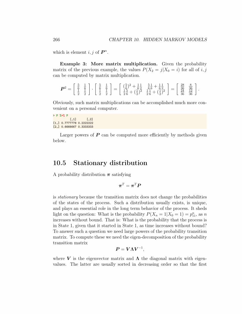
Example 3: More matrix multiplication. Given the probabilitymatrix of the previous example, the values P (X2 = j|X0 = i) for all of i, jcan be computed by matrix multiplication.

P 2 =

[56

16

12

12

]·[

56

16

12

12

]=

[(5

6)2 + 1

612

56

16

+ 16

12

12

56

+ (12)2 1

216

+ (12)2

]=

[2836

836

2436

1236

].

Obviously, such matrix multiplications can be accomplished much more con-venient on a personal computer.> P %*% P

[,1] [,2][1,] 0.7777778 0.2222222[2,] 0.6666667 0.3333333

Larger powers of P can be computed more efficiently by methods givenbelow.

10.5 Stationary distribution

A probability distribution π satisfying

πT = πTP

is stationary because the transition matrix does not change the probabilitiesof the states of the process. Such a distribution usually exists, is unique,and plays an essential role in the long term behavior of the process. It shedslight on the question: What is the probability P (Xn = 1|X0 = 1) = pn11, as nincreases without bound. That is: What is the probability that the process isin State 1, given that it started in State 1, as time increases without bound?To answer such a question we need large powers of the probability transitionmatrix. To compute these we need the eigen-decomposition of the probabilitytransition matrix

P = V ΛV −1,

where V is the eigenvector matrix and Λ the diagonal matrix with eigen-values. The latter are usually sorted in decreasing order so that the first

10.5. STATIONARY DISTRIBUTION 267

(left upper) is the largest. Now the third power of the probability transitionmatrix can be computed, as follows

P 3 = V ΛV −1V ΛV −1V ΛV −1 = V ΛΛΛV −1 = V Λ3V −1.

So that, indeed, in general

P n = V ΛnV −1.

The latter is a computationally convenient expression because we onlyhave to take the power of the eigenvalues in Λ and to multiply by the leftand right eigenvector matrices. We say that an n x n probability transitionmatrix P is diagonalizable when P has an eigen-decomposition - which is ifand only if P has n linearly independent eigenvectors.

In the long term the Markov process tends to a certain value (Brémaud,1999, p.197) because a probability transition matrix has a unique largesteigenvalue equal to 1 with corresponding eigenvectors 1 and π (or rathernormalized versions of these). It follows that, as n increases without bound,then P n tends to 1πT . In other words, P (Xn = j|X0 = i) = pnij tends toelement (i, j) of 1πT , which is equal to element j of π. For any initial dis-tribution π0, it follows that π′0P

n tends to πT .

Example 1: The stationary distribution. To compute the eigen-decomposition of the probability transition matrix P as well as powers of it,we may use the function eigen().> P <- matrix(c(1/6,5/6,0.5,0.5),2,2,byrow=T)> V <- eigen(P,symmetric = FALSE)> V$values[1] 1.0000000 -0.3333333> V$vectors

[,1] [,2][1,] -0.7071068 -0.8574929[2,] -0.7071068 0.5144958

The output of the function eigen() is assigned to the list V from whichthe eigenvalues and eigenvectors can be extracted and printed to the screen.Now we can compute P 16; the probability transition matrix raised to thepower sixteen.> V$vec %*% diag(V$va)^(16) %*% solve(V$vec)

[,1] [,2][1,] 0.375 0.625[2,] 0.375 0.625


So that the stationary distribution πT equals (0.375, 0.625).

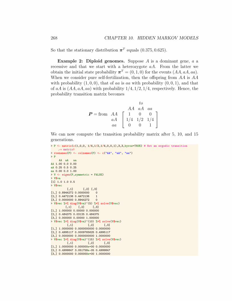
Example 2: Diploid genomes. Suppose A is a dominant gene, a arecessive and that we start with a heterozygote aA. From the latter weobtain the initial state probability πT = (0, 1, 0) for the events (AA, aA, aa).When we consider pure self-fertilization, then the offspring from AA is AAwith probability (1, 0, 0), that of aa is aa with probability (0, 0, 1), and thatof aA is (AA, aA, aa) with probability 1/4, 1/2, 1/4, respectively. Hence, theprobability transition matrix becomes

P = from AAaAaa

toAA aA aa 1 0 0

1/4 1/2 1/40 0 1

We can now compute the transition probability matrix after 5, 10, and 15generations.> P <- matrix(c(1,0,0, 1/4,1/2,1/4,0,0,1),3,3,byrow=TRUE) # Not an ergodic transition

↪→ matrix!> rownames(P) <- colnames(P) <- c("AA", "aA", "aa")> P

AA aA aaAA 1.00 0.0 0.00aA 0.25 0.5 0.25aa 0.00 0.0 1.00> V <- eigen(P,symmetric = FALSE)> V$va[1] 1.0 1.0 0.5> V$vec

[,1] [,2] [,3][1,] 0.8944272 0.0000000 0[2,] 0.4472136 0.4472136 1[3,] 0.0000000 0.8944272 0> V$vec %*% diag(V$va)^(5) %*% solve(V$vec)

[,1] [,2] [,3][1,] 1.000000 0.00000 0.000000[2,] 0.484375 0.03125 0.484375[3,] 0.000000 0.00000 1.000000> V$vec %*% diag(V$va)^(10) %*% solve(V$vec)

[,1] [,2] [,3][1,] 1.0000000 0.0000000000 0.0000000[2,] 0.4995117 0.0009765625 0.4995117[3,] 0.0000000 0.0000000000 1.0000000> V$vec %*% diag(V$va)^(15) %*% solve(V$vec)

[,1] [,2] [,3][1,] 1.0000000 0.000000e+00 0.0000000[2,] 0.4999847 3.051758e-05 0.4999847[3,] 0.0000000 0.000000e+00 1.0000000

10.6. PHYLOGENETIC DISTANCE 269

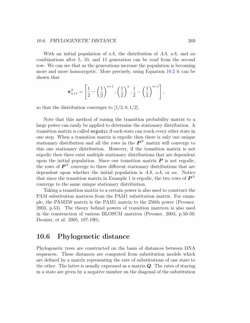
With an initial population of aA, the distribution of AA, aA, and aacombinations after 5, 10, and 15 generation can be read from the secondrow. We can see that as the generations increase the population is becomingmore and more homozygotic. More precisely, using Equation 10.2 it can beshown that

πTn+1 =

[1

2−(

1

2

)n+1

,

(1

2

)n,1

2−(

1

2

)n+1],

so that the distribution converges to [1/2, 0, 1/2].

Note that this method of raising the transition probability matrix to alarge power can easily be applied to determine the stationary distribution. Atransition matrix is called ergodic if each state can reach every other state inone step. When a transition matrix is ergodic then there is only one uniquestationary distribution and all the rows in the PN matrix will converge tothis one stationary distribution. However, if the transition matrix is notergodic then there exist multiple stationary distributions that are dependentupon the initial population. Since our transition matrix P is not ergodic,the rows of PN converge to three different stationary distributions that aredependent upon whether the initial population is AA, aA, or aa. Noticethat since the transition matrix in Example 1 is ergodic, the two rows of PN

converge to the same unique stationary distribution.Taking a transition matrix to a certain power is also used to construct the

PAM substitution matrices from the PAM1 substitution matrix. For exam-ple, the PAM250 matrix is the PAM1 matrix to the 250th power (Pevsner,2003, p.53). The theory behind powers of transition matrices is also usedin the construction of various BLOSUM matrices (Pevsner, 2003, p.50-59;Deonier, et al. 2005, 187-190).

10.6 Phylogenetic distance

Phylogenetic trees are constructed on the basis of distances between DNAsequences. These distances are computed from substitution models whichare defined by a matrix representing the rate of substitutions of one state tothe other. The latter is usually expressed as a matrixQ. The rates of stayingin a state are given by a negative number on the diagonal of the substitution


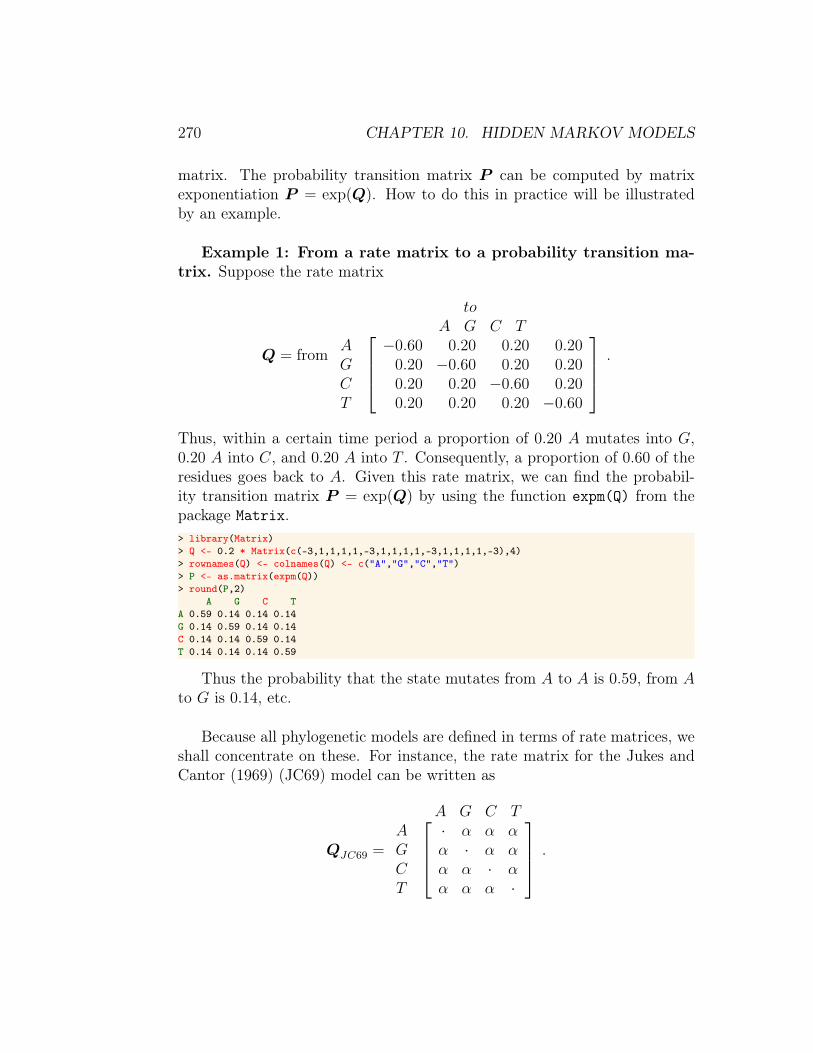
matrix. The probability transition matrix P can be computed by matrixexponentiation P = exp(Q). How to do this in practice will be illustratedby an example.

Example 1: From a rate matrix to a probability transition ma-trix. Suppose the rate matrix

Q = from AGCT

toA G C T

−0.60 0.20 0.20 0.200.20 −0.60 0.20 0.200.20 0.20 −0.60 0.200.20 0.20 0.20 −0.60

.

Thus, within a certain time period a proportion of 0.20 A mutates into G,0.20 A into C, and 0.20 A into T . Consequently, a proportion of 0.60 of theresidues goes back to A. Given this rate matrix, we can find the probabil-ity transition matrix P = exp(Q) by using the function expm(Q) from thepackage Matrix.> library(Matrix)> Q <- 0.2 * Matrix(c(-3,1,1,1,1,-3,1,1,1,1,-3,1,1,1,1,-3),4)> rownames(Q) <- colnames(Q) <- c("A","G","C","T")> P <- as.matrix(expm(Q))> round(P,2)

A G C TA 0.59 0.14 0.14 0.14G 0.14 0.59 0.14 0.14C 0.14 0.14 0.59 0.14T 0.14 0.14 0.14 0.59

Thus the probability that the state mutates from A to A is 0.59, from Ato G is 0.14, etc.

Because all phylogenetic models are defined in terms of rate matrices, weshall concentrate on these. For instance, the rate matrix for the Jukes andCantor (1969) (JC69) model can be written as

QJC69 =AGCT

A G C T· α α αα · α αα α · αα α α ·

.


The sum of each row of a rate matrix equals zero, so that from thisrequirement the diagonal elements of the JC69 model are equal to −3α.Furthermore, the non-diagonal substitution rates of the JC69 model all havethe same value α. That is, the mutate from i to j equals that from j to i,so that the rate matrix is symmetric. Also the probability that the sequenceequals one of the nucleotides is 1/4. This assumption, however, is unrealisticis many cases.

Transitions are substitutions of nucleotides within types of nucleotides,thus purine to purine or pyrmidine to pyrmidine (A ↔ G or C ↔ T ).Transversions are substitutions between nucleotide type (A ↔ T , G ↔T ,A ↔ C, and C ↔ G). In the JC69 model a transition is assumed tohappen with equal probability as a transversion. That is, it does not accountfor the fact that transitions are more common that transversions. To coverthis for more general type of models are proposed by Kimura (1980, 1981),which are commonly abbreviated by K80 and K81. In terms of the ratematrix these models can we written as

QK80 =

· α β βα · β ββ β · αβ β α ·

, QK81 =

· α β γα · γ ββ γ · αγ β α ·

In the K80 model a change within type (transition) occurs at rate α and

between type (transversion) at rate β. In the K81 model all changes occurat a different though symmetric rate; the rate of change A → G is α andequals that of A← G. If α is large, then the amount of transitions is large;if both β and γ are very small, then the number of transversions is small.

A model is called “nested” if it is a special case of a more general model.For instance, the K80 model is nested in the K81 model because when wetake γ = β, then we obtain the K80 model. Similarly, the JC69 model isnested in the K80 model because if we take β = α, then we obtain the JC69model.

Some examples of models with even more parameters are the Hasegawa,Kishino, and Yano (1985) (HKY85) model and the General Time-ReversableModel (GTR) model

QHKY 85 =

· απG βπC βπT

απA · βπC βπTβπA βπG · απTβπA βπG απC ·

, QGTR =

· απG βπC γπT

απA · δπC επTβπA δπG · ζπTγπA επG ζπC ·


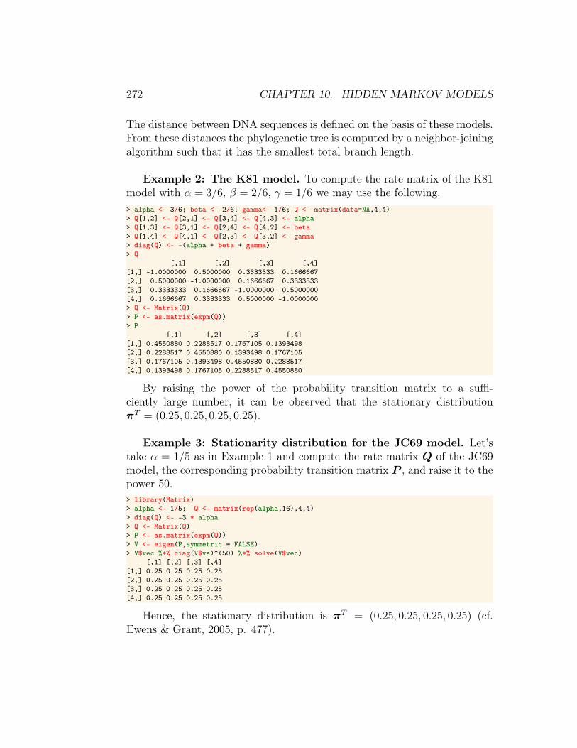
The distance between DNA sequences is defined on the basis of these models.From these distances the phylogenetic tree is computed by a neighbor-joiningalgorithm such that it has the smallest total branch length.

Example 2: The K81 model. To compute the rate matrix of the K81model with α = 3/6, β = 2/6, γ = 1/6 we may use the following.> alpha <- 3/6; beta <- 2/6; gamma<- 1/6; Q <- matrix(data=NA,4,4)> Q[1,2] <- Q[2,1] <- Q[3,4] <- Q[4,3] <- alpha> Q[1,3] <- Q[3,1] <- Q[2,4] <- Q[4,2] <- beta> Q[1,4] <- Q[4,1] <- Q[2,3] <- Q[3,2] <- gamma> diag(Q) <- -(alpha + beta + gamma)> Q

[,1] [,2] [,3] [,4][1,] -1.0000000 0.5000000 0.3333333 0.1666667[2,] 0.5000000 -1.0000000 0.1666667 0.3333333[3,] 0.3333333 0.1666667 -1.0000000 0.5000000[4,] 0.1666667 0.3333333 0.5000000 -1.0000000> Q <- Matrix(Q)> P <- as.matrix(expm(Q))> P

[,1] [,2] [,3] [,4][1,] 0.4550880 0.2288517 0.1767105 0.1393498[2,] 0.2288517 0.4550880 0.1393498 0.1767105[3,] 0.1767105 0.1393498 0.4550880 0.2288517[4,] 0.1393498 0.1767105 0.2288517 0.4550880

By raising the power of the probability transition matrix to a suffi-ciently large number, it can be observed that the stationary distributionπT = (0.25, 0.25, 0.25, 0.25).

Example 3: Stationarity distribution for the JC69 model. Let’stake α = 1/5 as in Example 1 and compute the rate matrix Q of the JC69model, the corresponding probability transition matrix P , and raise it to thepower 50.> library(Matrix)> alpha <- 1/5; Q <- matrix(rep(alpha,16),4,4)> diag(Q) <- -3 * alpha> Q <- Matrix(Q)> P <- as.matrix(expm(Q))> V <- eigen(P,symmetric = FALSE)> V$vec %*% diag(V$va)^(50) %*% solve(V$vec)

[,1] [,2] [,3] [,4][1,] 0.25 0.25 0.25 0.25[2,] 0.25 0.25 0.25 0.25[3,] 0.25 0.25 0.25 0.25[4,] 0.25 0.25 0.25 0.25

Hence, the stationary distribution is πT = (0.25, 0.25, 0.25, 0.25) (cf.Ewens & Grant, 2005, p. 477).


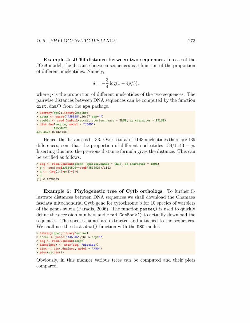
Example 4: JC69 distance between two sequences. In case of theJC69 model, the distance between sequences is a function of the proportionof different nucleotides. Namely,

d = −3

4log(1− 4p/3),

where p is the proportion of different nucleotides of the two sequences. Thepairwise distances between DNA sequences can be computed by the functiondist.dna() from the ape package.> library(ape);library(seqinr)> accnr <- paste("AJ5345",26:27,sep="")> seqbin <- read.GenBank(accnr, species.names = TRUE, as.character = FALSE)> dist.dna(seqbin, model = "JC69")

AJ534526AJ534527 0.1326839

Hence, the distance is 0.133. Over a total of 1143 nucleotides there are 139differences, som that the proportion of different nucleotides 139/1143 = p.Inserting this into the previous distance formula gives the distance. This canbe verified as follows.> seq <- read.GenBank(accnr, species.names = TRUE, as.character = TRUE)> p <- sum(seq$AJ534526==seq$AJ534527)/1143> d <- -log(1-4*p/3)*3/4> d[1] 0.1326839

Example 5: Phylogenetic tree of Cytb orthologs. To further il-lustrate distances between DNA sequences we shall download the Chamaeafasciata mitochondrial Cytb gene for cytochrome b for 10 species of warblersof the genus sylvia (Paradis, 2006). The function paste() is used to quicklydefine the accession numbers and read.GenBank() to actually download thesequences. The species names are extracted and attached to the sequences.We shall use the dist.dna() function with the K80 model.> library(ape);library(seqinr)> accnr <- paste("AJ5345",26:35,sep="")> seq <- read.GenBank(accnr)> names(seq) <- attr(seq, "species")> dist <- dist.dna(seq, model = "K80")> plot(nj(dist))

Obviously, in this manner various trees can be computed and their plotscompared.


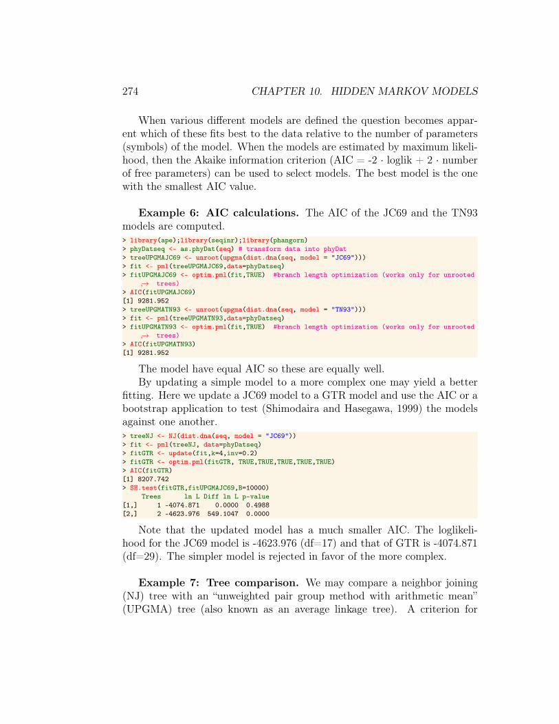
When various different models are defined the question becomes appar-ent which of these fits best to the data relative to the number of parameters(symbols) of the model. When the models are estimated by maximum likeli-hood, then the Akaike information criterion (AIC = -2 · loglik + 2 · numberof free parameters) can be used to select models. The best model is the onewith the smallest AIC value.

Example 6: AIC calculations. The AIC of the JC69 and the TN93models are computed.> library(ape);library(seqinr);library(phangorn)> phyDatseq <- as.phyDat(seq) # transform data into phyDat> treeUPGMAJC69 <- unroot(upgma(dist.dna(seq, model = "JC69")))> fit <- pml(treeUPGMAJC69,data=phyDatseq)> fitUPGMAJC69 <- optim.pml(fit,TRUE) #branch length optimization (works only for unrooted

↪→ trees)> AIC(fitUPGMAJC69)[1] 9281.952> treeUPGMATN93 <- unroot(upgma(dist.dna(seq, model = "TN93")))> fit <- pml(treeUPGMATN93,data=phyDatseq)> fitUPGMATN93 <- optim.pml(fit,TRUE) #branch length optimization (works only for unrooted

↪→ trees)> AIC(fitUPGMATN93)[1] 9281.952

The model have equal AIC so these are equally well.By updating a simple model to a more complex one may yield a better

fitting. Here we update a JC69 model to a GTR model and use the AIC or abootstrap application to test (Shimodaira and Hasegawa, 1999) the modelsagainst one another.> treeNJ <- NJ(dist.dna(seq, model = "JC69"))> fit <- pml(treeNJ, data=phyDatseq)> fitGTR <- update(fit,k=4,inv=0.2)> fitGTR <- optim.pml(fitGTR, TRUE,TRUE,TRUE,TRUE,TRUE)> AIC(fitGTR)[1] 8207.742> SH.test(fitGTR,fitUPGMAJC69,B=10000)

Trees ln L Diff ln L p-value[1,] 1 -4074.871 0.0000 0.4988[2,] 2 -4623.976 549.1047 0.0000

Note that the updated model has a much smaller AIC. The loglikeli-hood for the JC69 model is -4623.976 (df=17) and that of GTR is -4074.871(df=29). The simpler model is rejected in favor of the more complex.

Example 7: Tree comparison. We may compare a neighbor joining(NJ) tree with an “unweighted pair group method with arithmetic mean”(UPGMA) tree (also known as an average linkage tree). A criterion for


choosing between these two is a parsimoniousness score. The score can beoptimized by rearranging the trees.> treeUPGMAGG95 <- unroot(upgma(dist.dna(seq, model = "GG95"))) #plot(treeNJ)> treeUPGMAGG95 <- optim.parsimony(treeUPGMAGG95,phyDatseq)> parsimony(treeUPGMAGG95,phyDatseq)> treeNJGG95 <- NJ(dist.dna(seq, model = "GG95"))> treeNJGG95 <- optim.parsimony(treeNJGG95,phyDatseq)> parsimony(treeNJGG95,phyDatseq)

Both trees have score 570 and are equally parsimonious.

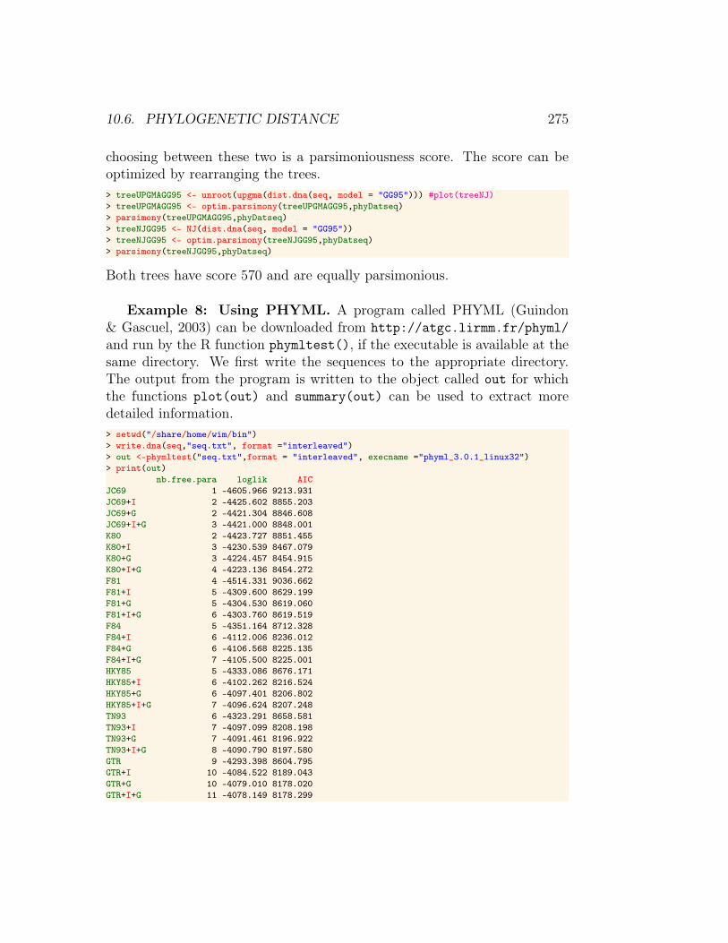
Example 8: Using PHYML. A program called PHYML (Guindon& Gascuel, 2003) can be downloaded from http://atgc.lirmm.fr/phyml/and run by the R function phymltest(), if the executable is available at thesame directory. We first write the sequences to the appropriate directory.The output from the program is written to the object called out for whichthe functions plot(out) and summary(out) can be used to extract moredetailed information.> setwd("/share/home/wim/bin")> write.dna(seq,"seq.txt", format ="interleaved")> out <-phymltest("seq.txt",format = "interleaved", execname ="phyml_3.0.1_linux32")> print(out)

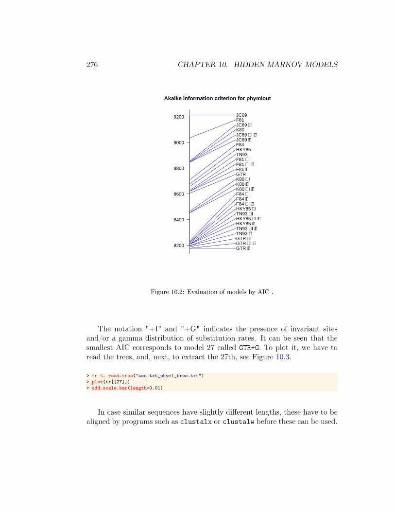
nb.free.para loglik AICJC69 1 -4605.966 9213.931JC69+I 2 -4425.602 8855.203JC69+G 2 -4421.304 8846.608JC69+I+G 3 -4421.000 8848.001K80 2 -4423.727 8851.455K80+I 3 -4230.539 8467.079K80+G 3 -4224.457 8454.915K80+I+G 4 -4223.136 8454.272F81 4 -4514.331 9036.662F81+I 5 -4309.600 8629.199F81+G 5 -4304.530 8619.060F81+I+G 6 -4303.760 8619.519F84 5 -4351.164 8712.328F84+I 6 -4112.006 8236.012F84+G 6 -4106.568 8225.135F84+I+G 7 -4105.500 8225.001HKY85 5 -4333.086 8676.171HKY85+I 6 -4102.262 8216.524HKY85+G 6 -4097.401 8206.802HKY85+I+G 7 -4096.624 8207.248TN93 6 -4323.291 8658.581TN93+I 7 -4097.099 8208.198TN93+G 7 -4091.461 8196.922TN93+I+G 8 -4090.790 8197.580GTR 9 -4293.398 8604.795GTR+I 10 -4084.522 8189.043GTR+G 10 -4079.010 8178.020GTR+I+G 11 -4078.149 8178.299


Akaike information criterion for phymlout

8200

8400

8600

8800

9000

9200

GTR + ΓGTR + I + ΓGTR + ITN93 + ΓTN93 + I + ΓHKY85 + ΓHKY85 + I + ΓTN93 + IHKY85 + IF84 + I + ΓF84 + ΓF84 + IK80 + I + ΓK80 + ΓK80 + IGTRF81 + ΓF81 + I + ΓF81 + ITN93HKY85F84JC69 + ΓJC69 + I + ΓK80JC69 + IF81JC69

Figure 10.2: Evaluation of models by AIC .

The notation "+I" and "+G" indicates the presence of invariant sitesand/or a gamma distribution of substitution rates. It can be seen that thesmallest AIC corresponds to model 27 called GTR+G. To plot it, we have toread the trees, and, next, to extract the 27th, see Figure 10.3.

> tr <- read.tree("seq.txt_phyml_tree.txt")> plot(tr[[27]])> add.scale.bar(length=0.01)

In case similar sequences have slightly different lengths, these have to bealigned by programs such as clustalx or clustalw before these can be used.

10.7. HIDDEN MARKOV MODELS 277

Chamaea fasciata

Sylvia nisoria

Sylvia layardi

Sylvia subcaeruleum

Sylvia boehmi

Sylvia buryi

Sylvia lugens

Sylvia leucomelaena

Sylvia hortensis

Sylvia crassirostris

0.01

Figure 10.3: Tree according to GTR model.

10.7 Hidden Markov Models

A Hidden Markov model (HMM) is a statistical Markov model in which thesystem being modeled is assumed to be a Markov process with unobserved,hidden states. Accordingly, in an HMM there are two probability transitionmatrices. There is an emission matrix E with probabilities of observed, emit-ted symbols and a transition matrix A with transition probabilities betweenthe unobserved, hidden states. The generation of an observable sequence re-quires two separate steps. First, there is a transition via a Markov process ofa hidden state and then given the new hidden state value there is an emissionof an observable outcome. We shall illustrate this by the classical example ofthe occasionally dishonest casino (Durbin et. al., 1998, p.18). The number


of hidden states and how they are connected (via transitions) defines thetopology of the HMM. For example, even though the dishonest casino andGC-isochore HMMs, that are defined below, model very different problems,they in fact share the same topology.

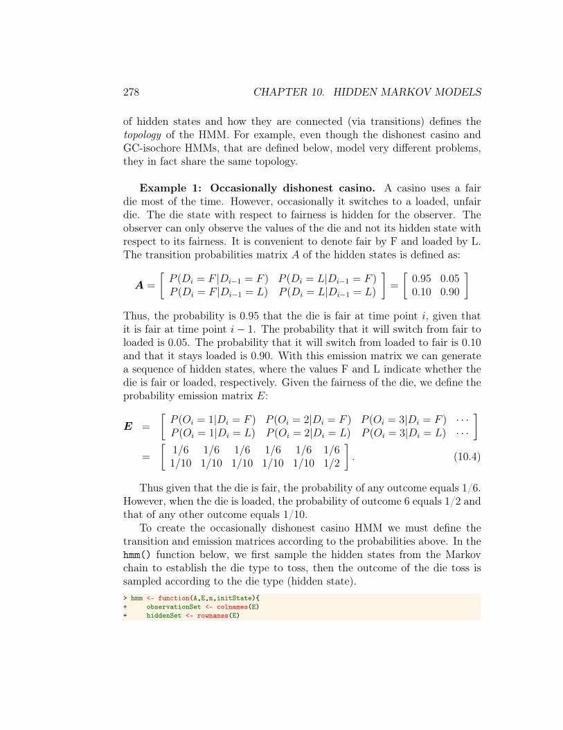
Example 1: Occasionally dishonest casino. A casino uses a fairdie most of the time. However, occasionally it switches to a loaded, unfairdie. The die state with respect to fairness is hidden for the observer. Theobserver can only observe the values of the die and not its hidden state withrespect to its fairness. It is convenient to denote fair by F and loaded by L.The transition probabilities matrix A of the hidden states is defined as:

A =

[P (Di = F |Di−1 = F ) P (Di = L|Di−1 = F )P (Di = F |Di−1 = L) P (Di = L|Di−1 = L)

]=

[0.95 0.050.10 0.90

]Thus, the probability is 0.95 that the die is fair at time point i, given thatit is fair at time point i− 1. The probability that it will switch from fair toloaded is 0.05. The probability that it will switch from loaded to fair is 0.10and that it stays loaded is 0.90. With this emission matrix we can generatea sequence of hidden states, where the values F and L indicate whether thedie is fair or loaded, respectively. Given the fairness of the die, we define theprobability emission matrix E:

E =

[P (Oi = 1|Di = F ) P (Oi = 2|Di = F ) P (Oi = 3|Di = F ) · · ·P (Oi = 1|Di = L) P (Oi = 2|Di = L) P (Oi = 3|Di = L) · · ·

]=

[1/6 1/6 1/6 1/6 1/6 1/61/10 1/10 1/10 1/10 1/10 1/2

]. (10.4)

Thus given that the die is fair, the probability of any outcome equals 1/6.However, when the die is loaded, the probability of outcome 6 equals 1/2 andthat of any other outcome equals 1/10.

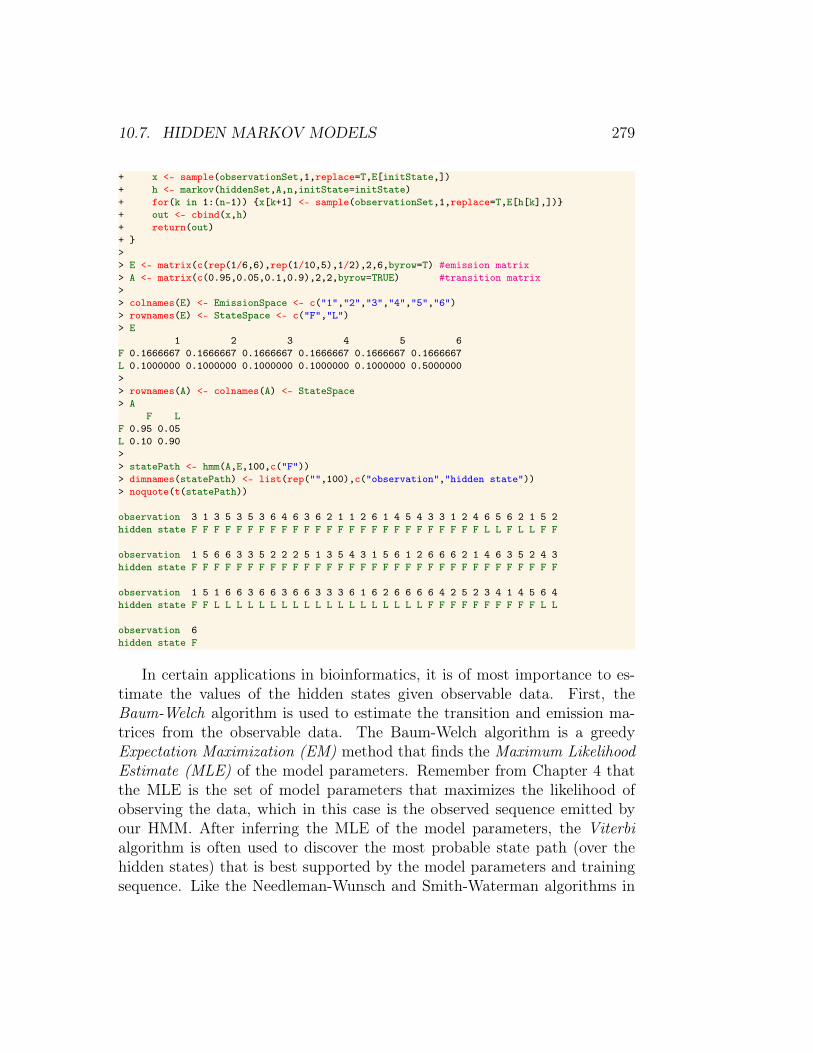
To create the occasionally dishonest casino HMM we must define thetransition and emission matrices according to the probabilities above. In thehmm() function below, we first sample the hidden states from the Markovchain to establish the die type to toss, then the outcome of the die toss issampled according to the die type (hidden state).> hmm <- function(A,E,n,initState){+ observationSet <- colnames(E)+ hiddenSet <- rownames(E)


+ x <- sample(observationSet,1,replace=T,E[initState,])+ h <- markov(hiddenSet,A,n,initState=initState)+ for(k in 1:(n-1)) {x[k+1] <- sample(observationSet,1,replace=T,E[h[k],])}+ out <- cbind(x,h)+ return(out)+ }>> E <- matrix(c(rep(1/6,6),rep(1/10,5),1/2),2,6,byrow=T) #emission matrix> A <- matrix(c(0.95,0.05,0.1,0.9),2,2,byrow=TRUE) #transition matrix>> colnames(E) <- EmissionSpace <- c("1","2","3","4","5","6")> rownames(E) <- StateSpace <- c("F","L")> E

1 2 3 4 5 6F 0.1666667 0.1666667 0.1666667 0.1666667 0.1666667 0.1666667L 0.1000000 0.1000000 0.1000000 0.1000000 0.1000000 0.5000000>> rownames(A) <- colnames(A) <- StateSpace> A

F LF 0.95 0.05L 0.10 0.90>> statePath <- hmm(A,E,100,c("F"))> dimnames(statePath) <- list(rep("",100),c("observation","hidden state"))> noquote(t(statePath))

observation 3 1 3 5 3 5 3 6 4 6 3 6 2 1 1 2 6 1 4 5 4 3 3 1 2 4 6 5 6 2 1 5 2hidden state F F F F F F F F F F F F F F F F F F F F F F F F F F L L F L L F F

observation 1 5 6 6 3 3 5 2 2 2 5 1 3 5 4 3 1 5 6 1 2 6 6 6 2 1 4 6 3 5 2 4 3hidden state F F F F F F F F F F F F F F F F F F F F F F F F F F F F F F F F F

observation 1 5 1 6 6 3 6 6 3 6 6 3 3 3 6 1 6 2 6 6 6 6 4 2 5 2 3 4 1 4 5 6 4hidden state F F L L L L L L L L L L L L L L L L L L L F F F F F F F F F F L L

observation 6hidden state F

In certain applications in bioinformatics, it is of most importance to es-timate the values of the hidden states given observable data. First, theBaum-Welch algorithm is used to estimate the transition and emission ma-trices from the observable data. The Baum-Welch algorithm is a greedyExpectation Maximization (EM) method that finds the Maximum LikelihoodEstimate (MLE) of the model parameters. Remember from Chapter 4 thatthe MLE is the set of model parameters that maximizes the likelihood ofobserving the data, which in this case is the observed sequence emitted byour HMM. After inferring the MLE of the model parameters, the Viterbialgorithm is often used to discover the most probable state path (over thehidden states) that is best supported by the model parameters and trainingsequence. Like the Needleman-Wunsch and Smith-Waterman algorithms in


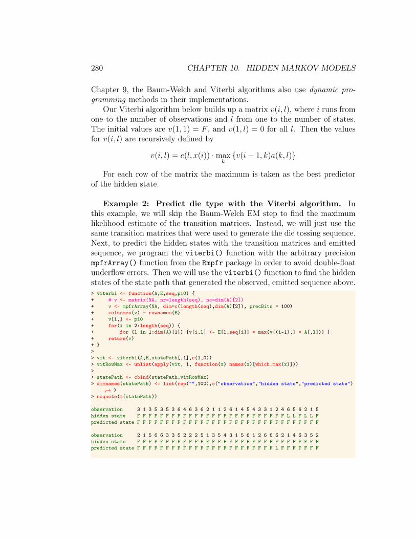
Chapter 9, the Baum-Welch and Viterbi algorithms also use dynamic pro-gramming methods in their implementations.

Our Viterbi algorithm below builds up a matrix v(i, l), where i runs fromone to the number of observations and l from one to the number of states.The initial values are v(1, 1) = F , and v(1, l) = 0 for all l. Then the valuesfor v(i, l) are recursively defined by

v(i, l) = e(l, x(i)) ·maxk{v(i− 1, k)a(k, l)}

For each row of the matrix the maximum is taken as the best predictorof the hidden state.

Example 2: Predict die type with the Viterbi algorithm. Inthis example, we will skip the Baum-Welch EM step to find the maximumlikelihood estimate of the transition matrices. Instead, we will just use thesame transition matrices that were used to generate the die tossing sequence.Next, to predict the hidden states with the transition matrices and emittedsequence, we program the viterbi() function with the arbitrary precisionmpfrArray() function from the Rmpfr package in order to avoid double-floatunderflow errors. Then we will use the viterbi() function to find the hiddenstates of the state path that generated the observed, emitted sequence above.> viterbi <- function(A,E,seq,pi0) {+ # v <- matrix(NA, nr=length(seq), nc=dim(A)[2])+ v <- mpfrArray(NA, dim=c(length(seq),dim(A)[2]), precBits = 100)+ colnames(v) = rownames(E)+ v[1,] <- pi0+ for(i in 2:length(seq)) {+ for (l in 1:dim(A)[1]) {v[i,l] <- E[l,seq[i]] * max(v[(i-1),] * A[,l])} }+ return(v)+ }>> vit <- viterbi(A,E,statePath[,1],c(1,0))> vitRowMax <- unlist(apply(vit, 1, function(x) names(x)[which.max(x)]))>> statePath <- cbind(statePath,vitRowMax)> dimnames(statePath) <- list(rep("",100),c("observation","hidden state","predicted state")

↪→ )> noquote(t(statePath))

observation 3 1 3 5 3 5 3 6 4 6 3 6 2 1 1 2 6 1 4 5 4 3 3 1 2 4 6 5 6 2 1 5hidden state F F F F F F F F F F F F F F F F F F F F F F F F F F L L F L L Fpredicted state F F F F F F F F F F F F F F F F F F F F F F F F F F F F F F F F

observation 2 1 5 6 6 3 3 5 2 2 2 5 1 3 5 4 3 1 5 6 1 2 6 6 6 2 1 4 6 3 5 2hidden state F F F F F F F F F F F F F F F F F F F F F F F F F F F F F F F Fpredicted state F F F F F F F F F F F F F F F F F F F F F F F F L F F F F F F F


observation 4 3 1 5 1 6 6 3 6 6 3 6 6 3 3 3 6 1 6 2 6 6 6 6 4 2 5 2 3 4 1 4hidden state F F F F L L L L L L L L L L L L L L L L L L L F F F F F F F F Fpredicted state F F F F F F F F F L L L L L L L L L L L L L L L L L L F F F F F

observation 5 6 4 6hidden state F L L Fpredicted state F F F F>> 1 - (sum(statePath[,2] == statePath[,3]) / nrow(statePath))[1] 0.16

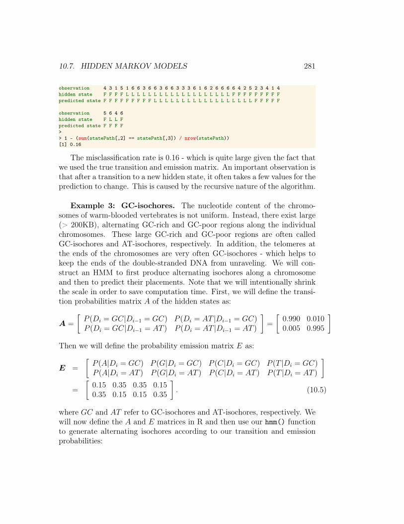
The misclassification rate is 0.16 - which is quite large given the fact thatwe used the true transition and emission matrix. An important observation isthat after a transition to a new hidden state, it often takes a few values for theprediction to change. This is caused by the recursive nature of the algorithm.

Example 3: GC-isochores. The nucleotide content of the chromo-somes of warm-blooded vertebrates is not uniform. Instead, there exist large(> 200KB), alternating GC-rich and GC-poor regions along the individualchromosomes. These large GC-rich and GC-poor regions are often calledGC-isochores and AT-isochores, respectively. In addition, the telomeres atthe ends of the chromosomes are very often GC-isochores - which helps tokeep the ends of the double-stranded DNA from unraveling. We will con-struct an HMM to first produce alternating isochores along a chromosomeand then to predict their placements. Note that we will intentionally shrinkthe scale in order to save computation time. First, we will define the transi-tion probabilities matrix A of the hidden states as:

A =

[P (Di = GC|Di−1 = GC) P (Di = AT |Di−1 = GC)P (Di = GC|Di−1 = AT ) P (Di = AT |Di−1 = AT )

]=

[0.990 0.0100.005 0.995

]Then we will define the probability emission matrix E as:

E =

[P (A|Di = GC) P (G|Di = GC) P (C|Di = GC) P (T |Di = GC)P (A|Di = AT ) P (G|Di = AT ) P (C|Di = AT ) P (T |Di = AT )

]=

[0.15 0.35 0.35 0.150.35 0.15 0.15 0.35

]. (10.5)

where GC and AT refer to GC-isochores and AT-isochores, respectively. Wewill now define the A and E matrices in R and then use our hmm() functionto generate alternating isochores according to our transition and emissionprobabilities:


> E <- matrix(c(0.15,0.35,0.35,0.15,+ 0.35,0.15,0.15,0.35),2,4,byrow=T) #emission matrix> A <- matrix(c(0.99,0.01,0.005,0.995),2,2,byrow=TRUE) #transition matrix>> colnames(E) <- EmissionSpace <- c("A","G","C","T")> rownames(E) <- StateSpace <- c("GC","AT")> E

A G C TGC 0.15 0.35 0.35 0.15AT 0.35 0.15 0.15 0.35> rownames(A) <- colnames(A) <- StateSpace> A

GC ATGC 0.990 0.010AT 0.005 0.995>> statePath <- hmm(A,E,1000,c("AT"))> dimnames(statePath) <- list(rep("",1000),c("observation","hidden state"))>> statePathFactor = factor(statePath[,2])> plot(x=1:length(statePathFactor), # 1 to n+ y=as.numeric(statePathFactor), # 1 or 2 based on factor+ type = "l", # line plot+ yaxt = "n", # do not plot y axis+ xlab = "Chromosome Location", # x-axis label+ ylab = "GC vs AT Isochores", # y-axis label+ col = "magenta", # color+ lwd = 2, # line width = 2+ cex.lab=1.5 # make axis labels big+ )> axis(2, at=c(1,2), labels=c("AT","GC"), cex.axis=1.5) # plot y-axis with special labels

The resulting plot of the generated isochores can be seen in Figure 10.4.Due to the transition probabilities, we see that the AT-isochores are generallylonger than the GC-isochores.

Example 4: Predict isochores with the Viterbi algorithm. Nowwe will use our viterbi() function to try to predict the placement of theisochores from the emitted sequence that was generated by our HMM:> vit <- viterbi(A,E,statePath[,1],c(0,1))> vitRowMax <- unlist(apply(vit, 1, function(x) names(x)[which.max(x)]))> vitRowMaxFactor = factor(vitRowMax)> plot(x=1:length(vitRowMaxFactor), # 1 to n+ y=as.numeric(vitRowMaxFactor), # 1 or 2 based on factor+ type = "l", # line plot+ yaxt = "n", # do not plot y-axis+ xlab = "Chromosome Location", # x-axis label+ ylab = "GC vs AT Isochores", # y-axis label+ col = "magenta", # line color+ lwd = 2, # line width+ cex.lab=1.5 # make axis labels big+ )> axis(2, at=c(1,2), labels=c("AT","GC"), cex.axis=1.5) # plot y-axis with special labels>> statePath <- cbind(statePath,vitRowMax)

10.8. APPENDIX 283

> dimnames(statePath) <- list(rep("",1000),c("observation","hidden state","predicted state"↪→ ))

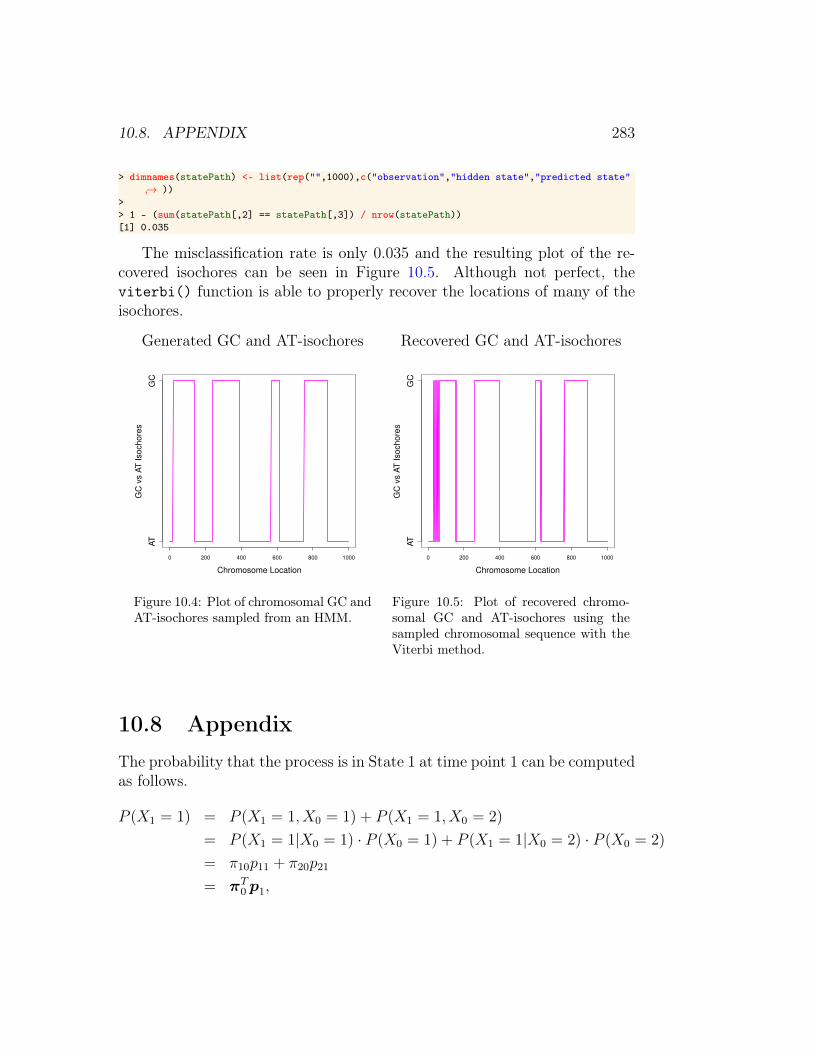
>> 1 - (sum(statePath[,2] == statePath[,3]) / nrow(statePath))[1] 0.035

The misclassification rate is only 0.035 and the resulting plot of the re-covered isochores can be seen in Figure 10.5. Although not perfect, theviterbi() function is able to properly recover the locations of many of theisochores.

Generated GC and AT-isochores

0 200 400 600 800 1000

Chromosome Location

GC

vs A

T Isochore

s

AT

GC

Figure 10.4: Plot of chromosomal GC andAT-isochores sampled from an HMM.

Recovered GC and AT-isochores

0 200 400 600 800 1000

Chromosome Location

GC

vs A

T Isochore

s

AT

GC

Figure 10.5: Plot of recovered chromo-somal GC and AT-isochores using thesampled chromosomal sequence with theViterbi method.

10.8 AppendixThe probability that the process is in State 1 at time point 1 can be computedas follows.

P (X1 = 1) = P (X1 = 1, X0 = 1) + P (X1 = 1, X0 = 2)

= P (X1 = 1|X0 = 1) · P (X0 = 1) + P (X1 = 1|X0 = 2) · P (X0 = 2)

= π10p11 + π20p21

= πT0 p1,


where p1 is the first column of P .In particular, it holds that

P (X2 = 1|X0 = 1) = P (X2 = 1, X1 = 1|X0 = 1) + P (X2 = 1, X1 = 2|X0 = 1)

=2∑

k=1

P (X2 = 1, X1 = k|X0 = 1)

=2∑

k=1

P (X2 = 1|X1 = k,X0 = 1) · P (X1 = k|X0 = 1)

=2∑

k=1

P (X2 = 1|X1 = k) · P (X1 = k|X0 = 1)

= p11p11 + p21p12

= row 1 of P times column 1 of P = P 211,

where the latter is element (1, 1) of the matrix P 2 = P · P .

10.9 Overview and concluding remarks

The probability transition matrix is extensively explained and illustratedbecause it is a cornerstone to many ideas in bioinformatics. A thoroughtreatment of phylogenetics is given by Paradis (2006) and of Hidden MarkovModels by Durbin et. al (2005).

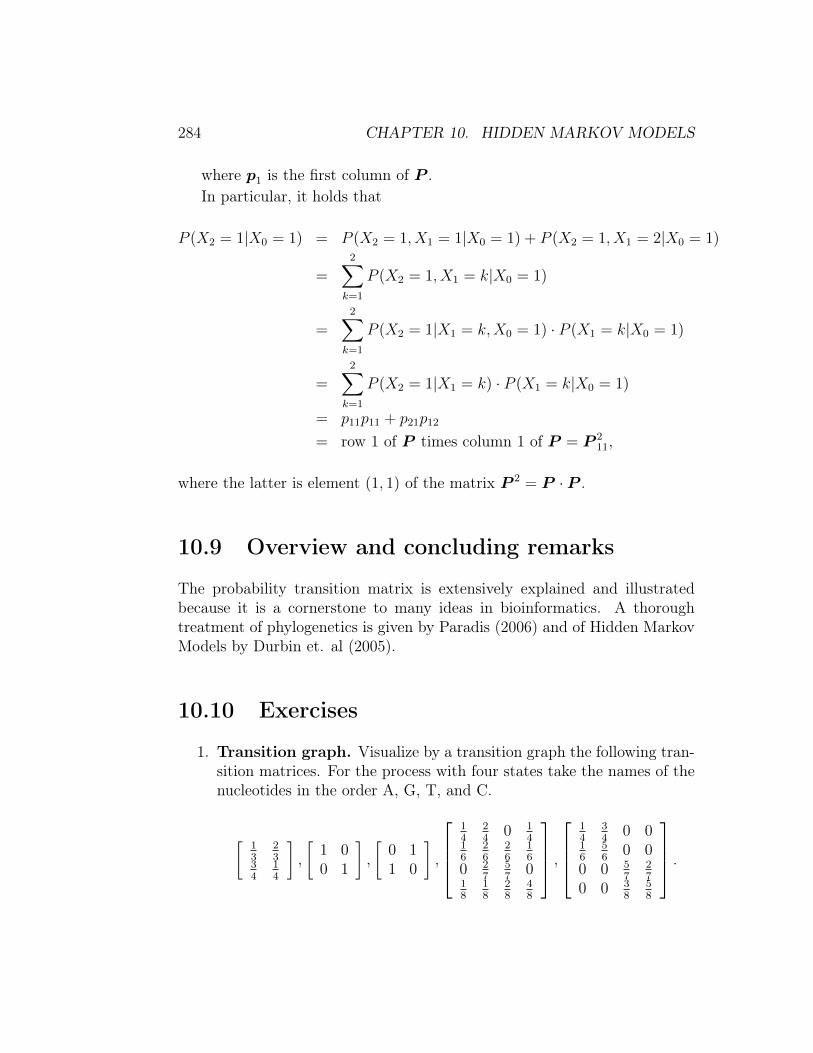
10.10 Exercises

1. Transition graph. Visualize by a transition graph the following tran-sition matrices. For the process with four states take the names of thenucleotides in the order A, G, T, and C.

[13

23

34

14

],

[1 00 1

],

[0 11 0

],

14

24

0 14

16

26

26

16

0 27

57

018

18

28

48

,

14

34

0 016

56

0 00 0 5

727

0 0 38

58

.

10.10. EXERCISES 285

2. Computing probabilities. Given the states 0 and 1 and the followinginitial distribution and probability matrix

π0 =[

12

12

],P =

[34

14

12

12

](a) Compute P (X1 = 0).

(b) Compute P (X1 = 1).

(c) Compute P (X2 = 0|X0 = 0).

(d) Compute P (X2 = 1|X0 = 0).

3. Programming GTR. Use πA = 0.15, πG = 0.35, πC = 0.35, πT =0.15, α = 4, β = 0.5, γ = 0.4, δ = 0.3, ε = 0.2, and ζ = 4.

(a) Program the rate matrix in such a manner that it is simple toadapt for other values of the parameters.

(b) Is the transversion rate larger or smaller then the transition rate?

(c) Compute the corresponding the probability transition matrix.

(d) Try to argue whether you expect a large frequency of transversionsor translations.

(e) Generate a sequence of 99 nucleotide residues according to themarkov model.

4. Distance according to JC69.

(a) Down load the sequences AJ534526 and AJ534527. Hint: Useas.character = TRUE in the read.GenBank() function.

(b) Compute the proportion of different nucleotides.

(c) Use this proportion to verify the distances between these sequencesaccording to the JC69 model.


Documents

Chapter10 HiddenMarkovModels - rileylab.orgrileylab.org/wp-content/uploads/2016/08/IntroBio... · Chapter10 HiddenMarkovModels TheMarkovprocessformsthebasisofmanyimportantmodelsinbioinfor-matics,