Embed Size (px)
Citation preview

8/6/2019 Chapter3 Environment Effects No Restriction
http://slidepdf.com/reader/full/chapter3-environment-effects-no-restriction 1/52

8/6/2019 Chapter3 Environment Effects No Restriction
http://slidepdf.com/reader/full/chapter3-environment-effects-no-restriction 2/52
ACKNOWLEDGMENT OF SPONSORSHIP
This work was sponsored by the American Association of State Highway and
Transportation Officials, in cooperation with the Federal Highway Administration, andwas conducted in the National Cooperative Highway Research Program, which is
administered by the Transportation Research Board of the National Research Council.
DISCLAIMER
This is the final draft as submitted by the research agency. The opinions and
conclusions expressed or implied in the report are those of the research agency. They are
not necessarily those of the Transportation Research Board, the National Research
Council, the Federal Highway Administration, the American Association of StateHighway and Transportation Officials, or the individual states participating in the
National Cooperative Highway Research Program.

8/6/2019 Chapter3 Environment Effects No Restriction
http://slidepdf.com/reader/full/chapter3-environment-effects-no-restriction 3/52
PART 2—DESIGN INPUTS
CHAPTER 3
ENVIRONMENTAL EFFECTS
2.3.1 INTRODUCTION
2.3.1.1 Importance of Climate in Mechanistic-Empirical Design
Environmental conditions have a significant effect on the performance of both flexible and rigid
pavements. External factors such as precipitation, temperature, freeze-thaw cycles, and depth towater table play a key role in defining the bounds of the impact the environment can have on the
pavement performance. Internal factors such as the susceptibility of the pavement materials to
moisture and freeze-thaw damage, drainability of the paving layers, infiltration potential of thepavement, and so on define the extent to which the pavement will react to the applied external
environmental conditions.
In a pavement structure, moisture and temperature are the two environmentally driven variables
that can significantly affect the pavement layer and subgrade properties and, hence, its load
carrying capacity. Some of the effects of environment on pavement materials are listed below:
• Asphalt bound materials exhibit varying modulus values depending on temperature.Modulus values can vary from 2 to 3 million psi or more during cold winter months to
about 100,000 psi or less during hot summer months.
• Cementitious material properties such as flexural strength and moduli are notsignificantly affected by normal temperature changes. However, temperature and
moisture gradients particularly in the top portland cement concrete (PCC) layer can
significantly affect stresses and deflections and consequently pavement damage anddistresses.
• At freezing temperatures, water in soil freezes and its resilient modulus could rise tovalues 20 to 120 times higher than the value of the modulus before freezing. Unbound
materials are not affected by temperature unless ice forms below 32oF.
• The freezing process may be accompanied by the formation of ice lenses that create
zones of greatly reduced strength in the pavement when thawing occurs.
• All other conditions being equal, the higher the moisture content the lower the modulusof unbound materials; however, moisture has two separate effects:
o First, it can affect the state of stress, through suction or pore water pressure.
Coarse grained and fine-grained materials can exhibit more than a fivefold
increase in modulus due to the soils drying out. The moduli of cohesive soils areaffected by clay-water-electrolyte interaction, which are fairly complex.
o Second, it can affect the structure of the soil through destruction of the
cementation between soil particles.
• Bound materials are not directly affected by the presence of moisture. However,excessive moisture can lead to stripping in asphalt mixtures or can have long-term effects
on the structural integrity of cement bound materials.
2.3.1

8/6/2019 Chapter3 Environment Effects No Restriction
http://slidepdf.com/reader/full/chapter3-environment-effects-no-restriction 4/52
• Cement bound materials may also be damaged during freeze-thaw and wet-dry cyclesreflected in modulus reduction and increased deflections. Freeze-thaw effects are
experienced in the underlying layers but eventually lead to distresses in the pavement
surface.
All the distresses considered in the Guide are affected by the environmental factors to somedegree. Therefore, diurnal and seasonal fluctuations in the moisture and temperature profiles in
the pavement structure brought about by changes in ground water table, precipitation/infiltration,freeze-thaw cycles, and other external factors are modeled in a very comprehensive manner in
this mechanistic-empirical design procedure.
2.3.1.2 Consideration of Climatic Effects in Design
The Enhanced Integrated Climatic Model
Changing temperature and moisture profiles in the pavement structure and subgrade over the
design life of a pavement are fully considered in the Design Guide approach through asophisticated climatic modeling tool called the Enhanced Integrated Climatic Model (EICM).The EICM is a one-dimensional coupled heat and moisture flow program that simulates changes
in the behavior and characteristics of pavement and subgrade materials in conjunction with
climatic conditions over several years of operation. The EICM consists of three majorcomponents:
• The Climatic-Materials-Structural Model (CMS Model) developed at the University of
Illinois (1).
• The CRREL Frost Heave and Thaw Settlement Model (CRREL Model) developed at the
United States Army Cold Regions Research and Engineering Laboratory (CRREL) (2).
• The Infiltration and Drainage Model (ID Model) developed at Texas A&M University(3).
The original version of the EICM, referred to simply as the Integrated Climatic Model, wasdeveloped for the Federal Highway Administration (FHWA) at Texas A&M University, Texas
Transportation Institute in 1989 (3). This version coupled the ID Model to the previously
developed CMS and CRREL Models, to develop an integrated environmental predictivemethodology. The original version was then modified and released in 1997 by Larson and
Dempsey as ICM version 2.0 (4). Additional modifications were performed in 1999, leading to
ICM version 2.1. Further improvements were made as part of the Design Guide development to
further improve the moisture prediction capabilities of ICM version 2.1. This version of the
program will be referred to henceforth as EICM. Overall, the EICM computes and predicts thefollowing information throughout the entire pavement/subgrade profile: temperature, resilient
modulus adjustment factors, pore water pressure, water content, frost and thaw depths, frostheave, and drainage performance. The model can be applied to either asphalt concrete (AC) or
PCC pavements.
2.3.2

8/6/2019 Chapter3 Environment Effects No Restriction
http://slidepdf.com/reader/full/chapter3-environment-effects-no-restriction 5/52
In developing the EICM, data from the Long Term Pavement Performance (LTPP) SeasonalMonitoring Program (SMP) test sections were used (5, 6, 7, 8). A detailed discussion on the
specific improvements can be obtained in Appendix DD and in References 5 through 8.
In short, the major tasks (relevant to the Design Guide) undertaken in developing EICM are:
• Replacement of the soil-water characteristic curve (SWCC) Gardner equation with the
equations proposed by Fredlund and Xing (9) to obtain a better functional fit.
• Development of improved estimates of SWCCs, saturated hydraulic conductivity (k sat ),and specific gravity of solids (G s) given known soil index properties such as grain-size
distribution (percent passing number 200 sieve, P 200, and effective grain size with 60percent passing by weight, D60) and Plasticity Index ( PI ).
• Incorporation into the EICM of an unsaturated hydraulic conductivity prediction based onthe SWCC proposed by Fredlund, et al. in 1994 (10).
• Addition of a climatic database containing hourly data from 800 weather stations from
across the United States for sunshine, rainfall, wind speed, air temperature, and relativehumidity. The data source was the National Climatic Data Center (NCDC).
The SWCC is defined as the variation of water storage capacity within the macro- and micro-pores of a soil, with respect to suction (11). This relationship is generally plotted as the variation
of the water content (gravimetric, volumetric, or degree of saturation) with soil suction. Several
mathematical equations have been proposed to represent the SWCC. The ICM version 2.1 made
use of the equation proposed by Gardner in 1958 that has been shown, in many cases, tomisrepresent the SWCC due to excessive constraints to the relationship. Several studies have
been conducted on comparing the different equations available to represent the SWCC (12, 13).
Those studies have generally shown that the equations proposed by Fredlund and Xing in 1994
(9) showed good agreement with an extended database. For this reason, the Fredlund and Xingequation is used in the Design Guide procedure.
Another important improvement of practical relevance was the introduction of algorithms to
estimate the specific gravity of the solids (G s) and the saturated hydraulic conductivity (k sat ).
These estimations can be used in cases where G s and k sat cannot be estimated from field or
laboratory testing (i.e., they can be used at input Level 2). The G s and the k sat are both estimatedbased on P200, PI, and D60 values.
The next major modification was the incorporation of an algorithm to predict the unsaturatedhydraulic conductivity. The ICM version 2.1 made use of the Gardner's parameters for the
representation of the unsaturated hydraulic conductivity function, which is the relationshipbetween hydraulic conductivity and soil matric suction. As part of the modifications performedto the ICM version 2.1, the unsaturated hydraulic conductivity default parameters were replaced
by the equation proposed by Fredlund et al. in 1994 (10). The proposed hydraulic conductivity
function is an integral form of the water content versus suction relationship and makes use of theSWCC fitting parameters proposed by the same researchers.
2.3.3

8/6/2019 Chapter3 Environment Effects No Restriction
http://slidepdf.com/reader/full/chapter3-environment-effects-no-restriction 6/52
The last major modification to the ICM version 2.1 was the incorporation of data from over 800weather stations across the United States. The information was obtained from the NCDC and
contains hourly variations of several variables used to establish the temperature, moisture, and
frost regimes within a pavement structure virtually anywhere in the country. This enhancementconsiderably enhances the quality of the design procedure.
Incorporation of EICM into the Design Guide
The EICM software has been made an integral part of the Design Guide procedure. It is fully
linked to the software accompanying the Design Guide and internally performs all the necessary
computations. The user inputs to the EICM are entered through interfaces provided as part of theDesign Guide software. The EICM processes these inputs and feeds the processed outputs to the
three major components of the Design Guide’s mechanistic-empirical design framework—
materials, structural responses, and performance prediction. Thus, climate is fully incorporated
into the Design Guide methodology, which will provide improved capabilities in pavementdesign.
The tasks listed in the following paragraph summarize the role of the EICM module in theoverall design process. For flexible pavement analysis and design, the tasks incorporated to
account for the environmental effects include the following:
Task 1 Records the user supplied resilient modulus, M R, of all unbound layer materials at an
initial or reference condition. Generally, this will be at or near the optimum water
content and maximum dry density. PART 2, Chapter 2 discusses how M R can be
estimated at the various hierarchical input levels.
Task 2 Evaluates the expected changes in moisture content, from the initial or reference
condition, as the subgrade and unbound materials reach equilibrium moisturecondition. Also evaluates the seasonal changes in moisture contents.
Task 3 Evaluates the effect of changes in soil moisture content with respect to the reference
condition on the user entered resilient modulus, M R.
Task 4 Evaluates the effect of freezing on the layer M R.
Task 5 Evaluates the effect of thawing and recovery from the frozen M R condition.
Task 6 Utilization of time—varying M R values in the computation of critical pavement
response parameters and damage at various points within the pavement system.
Task 7 Evaluate changes in temperature as a function of time for all asphalt bound layers.
The input in Task 1, M Ropt , (M R at optimum compaction conditions and the chosen referencevalue), is a materials-related entry provided by the user (described in PART 2, Chapter 2). This
value is determined using either the Finite Element Analysis (FEA) procedure or the Linear
2.3.4

8/6/2019 Chapter3 Environment Effects No Restriction
http://slidepdf.com/reader/full/chapter3-environment-effects-no-restriction 7/52
Elastic Analysis (LEA) procedure consistent with the Design Guide, depending on whetherstress-dependent moduli or linear elastic analysis is utilized.
Tasks 2 through 7 are performed internally by the EICM embedded into the Design Guidesoftware and the outputs are made available to both the flexible and rigid pavement design
modules.
For rigid pavements, the following additional tasks are performed by the EICM:
Task 8 Generate temperature profiles in the PCC and underlying layers for the trial design
section for each hour of each day for the selected location using the weather stationinformation (used for thermal gradients in PCC, joint and crack openings and
closings, and AC base temperatures for modulus estimation).
Task 9 Convert the non-linear temperature profile to an effective linear temperature gradient
that is used to model slab curvature and thermal stresses.
Task 10 Generate a probability distribution file of effective linear temperature gradients that
can be expected to occur for each month of the year for the trial design cross section.
Task 11 Determine the freezing index and the number of freeze-thaw cycles for the selectedlocation.
Task 12 Provide mean monthly relative humidity values for use in estimating the moisturewarping of the PCC slabs on a monthly basis.
One of the important outputs required from the EICM for the flexible and rigid pavement design
is a set of adjustment factors for unbound material layers that account for the effects of
environmental parameters and conditions such as moisture content changes, freezing, thawing,and recovery from thawing. This factor, denoted F env, varies with position within the pavement
structure and with time throughout the analysis period. The F env factor is a coefficient that is
multiplied by the M Ropt to obtain M R as a function of position and time.
Three additional outputs of importance from the EICM are the in-situ temperatures at the
midpoints of each bound sublayer (with statistics that quantify the variability), the temperature
profiles within the AC and/or PCC layer for every hour, and the average moisture content foreach sublayer in the pavement structure. These outputs are described in the next subsection.
2.3.1.3 Major Outputs of the EICM
Following is a summary of the major outputs of the EICM and the ways they are used in Design
Guide methodology. The output of the EICM can be described on two levels—internal andexternal. Both forms of outputs of the EICM are transparent to the user with the difference being
that the internal outputs are not passed on to other components of the Design Guide software
(e.g., structural response calculation module or the performance prediction module), while the
2.3.5

8/6/2019 Chapter3 Environment Effects No Restriction
http://slidepdf.com/reader/full/chapter3-environment-effects-no-restriction 8/52
external outputs are. However, the user has full control over the inputs that drive both theseoutputs (e.g., water table depths, climatic information for the project site).
Internal Output of the EICM
The computational engine of the EICM determines values of volumetric water content, θ w, andtemperature at each node over time based on certain user inputs discussed later in this Chapter.
The values of θ w are divided by the saturated volumetric water contents, θ sat , to get values of degree of saturation, S . With no oscillations in the input groundwater table and no cracks in the
AC layer, values of S are essentially values at a state of equilibrium, S equil , unless freezing or
thaw recovery is in progress.
Values of S equil , together with values of degree of saturation at optimum conditions, S opt , are then
used to compute the unbound layer modulus adjustment factor for unfrozen conditions, F U , at
each node. The output temperatures are used to signal freezing at a node and an adjustmentfactor for frozen condition, F F , is computed at each freezing node. Thawing normally follows
freezing, as signaled by the rise in temperature above the freezing point. During the recoveryperiod, material type/properties are used to compute the recovery ratio, RR, at recovering nodes.These RR values, together with reduction factors due to thawing, RF , are used to compute and
adjustment factor for recovering conditions, F R, at each recovering node.
External Output of the EICM
The following outputs are generated by EICM for use by other components of the Design Guide
software:
• Unbound material M R adjustment factor as function of position and time—values of
composite environmental effects adjustment factor, F env, are computed for every sublayerfrom the values of F F , F R, or F U at each node. The sublayering is internally defined bythe EICM and is a function of the frost penetration depth, among other factors. These
F env factors are sent forward either to the FEA or to the LEA structural analysis modules
of the Design Guide software, where they are multiplied by M Ropt to obtain M R asfunction of position and time.
• Temperatures at the surface and at the midpoint of each asphalt bound sublayer—thesevalues are subjected to statistical characterization for every analysis period (1 month or
2-week period). The mean, standard deviation, and quintile points are sent forward foruse in the fatigue and permanent deformation prediction models.
• Values of hourly temperature at the surface and at a set depth increment (every inch)
within the bound layers for use in the thermal cracking model.• Volumetric moisture content—an average value for each sublayer is reported for use in
the permanent deformation model for the unbound materials.
• Temperature profile in the PCC—hourly values are generated for use in the cracking andfaulting models for jointed plain concrete pavement (JPCP) and the punchout model for
continuously reinforced concrete pavement (CRCP).
• Number of freeze thaw cycles and freezing index are computed for use in JPCPperformance prediction.
2.3.6

8/6/2019 Chapter3 Environment Effects No Restriction
http://slidepdf.com/reader/full/chapter3-environment-effects-no-restriction 9/52
• Relative humidity values for each month are generated for use in the JPCP and CRCPmodeling of moisture gradients through the slab.
The external EICM outputs feed directly into the materials characterization, structural response
computation, and performance prediction modules of the Design Guide software.
2.3.1.4 Chapter Organization
A majority of this chapter is devoted to guiding the user through the process of generating theinputs needed for the EICM at the various hierarchical levels. Although the algorithms used for
computing modulus adjustment factors, F env, are internal to the EICM, considerable discussion is
provided towards the end of the chapter to explain how these computations are made.Discussion on how EICM determines the temperature and moisture distribution within the
pavement system is also included in this chapter.
2.3.2 CLIMATIC AND MATERIAL INPUTS REQUIRED TO MODEL THERMAL AND
MOISTURE CONDITIONS
A relatively large number of input parameters are needed to produce the desired outputs from theEICM for pavement design. As with other inputs discussed so far in PART 2 of the Guide, even
inputs to the climatic model can be provided at any of the hierarchical levels (1, 2, or 3) to
provide flexibility in implementation of the Design Guide. The inputs required by the climaticmodel fall under the following broad categories:
• General information.
• Weather-related information.
• Ground water related information.
• Drainage and surface properties.
• Pavement structure and materials.
The ensuing discussion presents the specific inputs required under each of the above mentionedcategories and the recommended procedures to obtain them at the various hierarchical input
levels. The relevance of each of these inputs to pavement design is also noted, where applicable.The discussion presented covers both new and rehabilitation design.
Note that there is some overlap between the inputs discussed in this chapter and those discussedin PART 2, Chapters 1 and 2 as well as PART 3, Chapters 3, 4, 6, and 7. This is anticipated
since the influence of climate on pavement performance is intimately linked with the materials,
layer structure, and design features being considered in the trial design. The interaction betweenclimate, materials, and pavement design is fully explored in the Design Guide.
2.3.7

8/6/2019 Chapter3 Environment Effects No Restriction
http://slidepdf.com/reader/full/chapter3-environment-effects-no-restriction 10/52
2.3.2.1 General Information
Under this category, the following inputs specifically relate to the climatic model:
• Base/Subgrade Construction Completion Month and Year —This input is required fornew flexible pavement design only. It is required to initialize the moisture model in the
EICM. The moisture calculations in the unbound materials start from this point in time
and as the moisture contents in these layers change from the optimum values input by the
user to an equilibrium value, the layer moduli are adjusted accordingly. When taken inconjunction with the traffic open month, this input is also used to control the length of the
analysis period. For example, if the time difference between the construction month and
the traffic open month is 2 years and the anticipated design life is 20 years, the analysisperiod is set to 22 years. If this input is completely unknown, the designer should use the
month that most highway construction occurs in the area.
• Existing Pavement Construction Month and Year —This input is required only for
rehabilitation design using both AC and PCC overlays. If the underlying pavement is aflexible pavement, this parameter helps identify the extent to which the pavement is aged
at the time of rehabilitation. If the underlying pavement is a rigid pavement, this
parameter is used to estimate the strength and modulus of the PCC layer at the time of rehabilitation. If this input is completely unknown, the designer should use the month that
most highway construction occurs in the area.
• Pavement Construction Month and Year —This parameter is required for both new and
rehabilitation design. For flexible pavement design, this parameter helps determine thestiffness and strength characteristics of the asphalt layer and for rigid pavement design it
is used to estimate the “zero-stress” temperature in the PCC at construction. The zero-
stress temperature affects JPCP faulting and CRCP punchout predictions (see PART 3,Chapter 4 for more discussion on this input). Further, in CRCP design, this input is used
to compute relative humidities, which have an impact on initial crack spacing and width.
If this input is completely unknown, the designer should use the month that mosthighway construction occurs in the area.
• Traffic Opening Month and Year —The expected month in which the pavement will be
opened to traffic after construction. This value defines the climatic conditions at the timeof opening to traffic, which relates to the temperature gradients and the layer moduli,including that of the subgrade. If completely unknown, the designer should use the most
likely month after the estimated construction month.
• Type of Design—New or Rehabilitation and AC or PCC. This input determines the types
of climatic user inputs required for the analysis, climatic model initialization parameters,
pavement sublayering schemes, types of outputs required from climatic analysis, and so
on.
2.3.8

8/6/2019 Chapter3 Environment Effects No Restriction
http://slidepdf.com/reader/full/chapter3-environment-effects-no-restriction 11/52
2.3.2.2 Weather-Related Data
To accomplish the climatic analysis required for incremental damage accumulation, the Design
Guide approach requires information on the following five weather-related parameters on anhourly basis over the entire design life for the project being designed:
• Hourly air temperature.
• Hourly precipitation.
• Hourly wind speed.
• Hourly percentage sunshine (used to define cloud cover).
• Hourly relative humidity.
The air temperature is required by the heat balance equation in the EICM for calculations of long
wave radiation emitted by the air and for the convective heat transfer from surface to air. Both
computations are explained in detail later in this chapter. In addition to the heat calculations, the
temperature data is used to define the frozen/thawing periods within the analysis time frame andto determine the number of freeze-thaw cycles.
Heat fluxes resulting from precipitation and infiltration into the pavement structure have not
been considered in formulating the surface heat flux boundary conditions. The role of the
precipitation under these circumstances in not entirely clear, and methods to incorporate it in theenergy balance have not been attempted. However, precipitation is needed to compute
infiltration for rehabilitated pavements and aging processes. Furthermore, the precipitation that
falls during a month when the mean temperature is less than the freezing temperature of water is
assumed to fall as snow.
Wind speed is required in the computations of the convention heat transfer coefficient at thepavement surface. The percentage sunshine is needed for the calculations of heat balance at thesurface of the pavement. Both calculations are described in detail later on in this chapter.
Hourly relative humidities have a big impact on drying shrinkage of JPCP and CRCP and also indetermining the crack spacing and initial crack width in CRCP. The role ambient relative
humidity plays in determining these parameters is described in more detail in PART 3, Chapter
4, as well as in the related appendices.
Determination of Weather-Related Parameters
In the Design Guide approach, the weather-related information is primarily obtained fromweather stations located near the project site. The software accompanying the Design Guide has
an available database from nearly 800 weather stations throughout the United States. Several of
the major weather stations have approximately 60 to 66 months of climatic data at each time step(1 hour) needed by the EICM. Other weather stations could have less than this amount of data,
however, the Design Guide software requires at least 24 months of actual weather station data for
computational purposes.
2.3.9

8/6/2019 Chapter3 Environment Effects No Restriction
http://slidepdf.com/reader/full/chapter3-environment-effects-no-restriction 12/52
The climatic database can be tapped into by simply specifying the latitude, longitude, andelevation of the project site. Once the coordinates and elevation are specified, the Design Guide
software will highlight the six closest weather stations to the site from which the user may select
any number of stations to create a virtual project weather station. Because there could be somemissing data in each actual weather station data file, it is recommended that as many stations be
combined as possible to allow data smoothing and ensure adequate information (recall that aminimum of 24 months of climatic data is required) . The EICM will show the distance betweenthe site and each highlighted weather station and the amount of information (number of months)
available for each one of these stations. After the appropriate number of representative weather
stations is chosen, interpolation of climatic data from these stations is done and the interpolated
data is made available for storage as a virtual weather station. The climatic data from virtualweather stations created in this manner will be made use of by the Design Guide software to
assess temporal changes in material behavior, computing structural responses due to
environmental loads, and to predict pavement distress.
The configuration of weather-related information required for design is the same at all the three
hierarchical input levels. Interpolation of climatic information from as many applicable weatherstations as possible for a given project site is recommended to smooth erroneous data or to fill in
missing information.
2.3.2.3 Groundwater Table Depth
The groundwater table depth is intended to be either the best estimate of the annual average
depth or the seasonal average depth (a value for each of the four seasons of the year). At inputLevel 1, it could be determined from profile characterization borings prior to design. At input
Level 3, an estimate of the annual average value or the seasonal averages can be provided. Apotential source to obtain Level 3 estimates is the county soil reports produced by the National
Resources Conservation Service (14).
It is important to recognize that this parameter plays a significant role in the overall accuracy of
the foundation/pavement moisture contents and, hence, equilibrium modulus values. Every
attempt should be made to characterize it as accurately as possible.
2.3.2.4 Drainage and Surface Properties
Surface Shortwave Absorptivity
This input pertains to the AC and PCC surface layers. The surface short wave absorptivity of a
given layer depends on its composition, color, and texture. This quantity directly correlates withthe amount of available solar energy that is absorbed by the pavement surface. Generally
speaking, lighter and more reflective surfaces tend to have lower short wave absorptivity and
vice versa.
2.3.10

8/6/2019 Chapter3 Environment Effects No Restriction
http://slidepdf.com/reader/full/chapter3-environment-effects-no-restriction 13/52
The following are the recommended ways to the estimate this parameter at each of thehierarchical input levels:
• Level 1 – At this level it is recommended that this parameter be estimated through
laboratory testing. However, although there are procedures in existence to measure
shortwave absorptivity, there are no current AASHTO certified standards for pavingmaterials.
• Level 2 – Not applicable.
• Level 3 – At Level 3, default values can be assumed for various pavement materials asfollows:
o Weathered asphalt (gray) 0.80 – 0.90
o Fresh asphalt (black) 0.90 – 0.98
o Aged PCC layer 0.70 – 0.90
Infiltration
This parameter defines the net infiltration potential of the pavement over its design life. In theDesign Guide approach, infiltration can assume four values – none, minor (10 percent of the
precipitation enters the pavement), moderate (50 percent of the precipitation enters the
pavement), and extreme (100 percent of the precipitation enters the pavement). Based on this
input, the EICM determines the amount of water available on top of the first unbound layer.
Most designs and maintenance activities, especially on higher functional class pavements, should
strive to achieve zero infiltration or reduce it to a minimum value. This can be done by properdesign of surface drainage elements (cross-slopes, side ditches, etc.), adopting construction
practices that reduce infiltration (e.g., eliminating cold lane/shoulder joints, tied joints in the case
of PCC pavements, etc.), proactive routine maintenance activities (e.g., crack and joint sealing,
surface treatments, etc.), and providing adequate subsurface drainage in the form of drainagelayers or edgedrains. Using moisture insensitive materials can also mitigate the impact of any
moisture that infiltrates the pavement. PART 3, Chapter 1 provides more discussion on how toreduce pavement infiltration.
The amount of infiltration into the pavement at any given point in time due to a certain rain event
is a function of the pavement condition, shoulder type, and drainage features the intercept the
moisture. For simplicity, the general guidelines for estimating infiltration are based only on the
shoulder type and if edgedrains are present or not. The shoulder type is relevant since the lane-shoulder joint represents the largest single source of moisture entry into the pavement structure.
The presence of edgedrains is relevant since they shorten the drainage path and provide a
positive drainage outlet. Note that if a drainage layer is present in addition to edgedrains, itsimpact on protecting the underlying layers from getting saturated is automatically accounted for
within the EICM through a direct modeling of how this layer impacts the modulus of unbound
layers and subgrade.
2.3.11
8/6/2019 Chapter3 Environment Effects No Restriction
http://slidepdf.com/reader/full/chapter3-environment-effects-no-restriction 14/52
The following recommendations are made for selecting the Infiltration input parameter:
• Minor – This option is valid when tied and sealed concrete shoulders (in rigidpavements), widened PCC lanes, or full width AC paving (monolithic main lane and
shoulder) are used or when an aggressive policy is pursued to keep the lane-shoulder joint
sealed. This option is also applicable when edgedrains are used.• Moderate – This option is valid for all other shoulder types, PCC restoration, and ACoverlays over old and cracked existing pavements where reflection cracking will likely
occur.
• Extreme – Generally not used for new or reconstructed pavement design.
These recommendations are valid at all the hierarchical input levels.
Drainage Path Length
The drainage path length is the resultant length of the drainage path, i.e., the distance measured
along the resultant of the cross and longitudinal slopes of the pavement. It is measured fromhighest point in the pavement cross-section to the point where drainage occurs. This input is
used in the EICM’s infiltration and drainage model to compute the time required to drain an
unbound base or subbase layer from an initially wet condition.
The DRIP microcomputer program (explained in Appendix TT and available as part of the
Design Guide software) can be used to compute this parameter based on pavement cross and
longitudinal slopes, lane widths, edgedrain trench widths (if applicable), and cross-sectiongeometry (crowned or superelevated).
Pavement Cross-Slope
The cross slope is the slope of the pavement surface perpendicular to the direction of traffic.
This input is used in computing the time required to drain a pavement base or subbase layer froman initially wet condition.
2.3.2.5 Pavement Structure Materials Inputs
Layer Thicknesses
The layer thickness of each material in the pavement structure should correspond to layers that
are more or less homogeneous. EICM internally subdivides these layers for more accurate
calculations of moisture and temperature profiles. The procedure always requires two unboundlayers under the last stabilized layer for computational purposes (e.g., one layer could be
compacted subgrade and the other the natural subgrade, or one layer could be compacted
granular fill and the other natural subgrade). If the trial design does not facilitate this, thesubgrade layer is subdivided into two layers internally by the Design Guide software. Further,
all layer subdivisions are handled internally and automatically. The user should not subdivide
the pavement layers into sublayers. A description of sublayering and its relevance in computingseasonal pavement moduli is provided in PART 3, Chapter 3.
2.3.12

8/6/2019 Chapter3 Environment Effects No Restriction
http://slidepdf.com/reader/full/chapter3-environment-effects-no-restriction 15/52
Asphalt Material Properties
Several asphalt properties are required for the design of flexible pavements and AC overlays.
Among these properties are those that control the heat flow through the pavement system andthereby influence the temperature and moisture regimes within it. Asphalt material properties
that enter the EICM calculations include:
• Surface shortwave absorptivity.
• Thermal conductivity, K .
• Heat or thermal capacity, Q.
Shortwave absorptivity has been discussed earlier in this chapter. Therefore, the discussion
under this section is restricted to thermal conductivity and heat capacity.
Thermal conductivity, K , is the quantity of heat that flows normally across a surface of unit area
per unit of time and per unit of temperature gradient. The moisture content has an influence
upon the thermal conductivity of asphalt concrete. If the moisture content is small, thedifferences between the unfrozen, freezing and frozen thermal conductivity are small. Only
when the moisture content is high (e.g., greater than 10%) does the thermal conductivity vary
substantially. The EICM does not vary the thermal conductivity with varying moisture content
of the asphalt layers as it does with the unbound layers.
The heat or thermal capacity is the actual amount of heat energy Q necessary to change the
temperature of a unit mass by one degree.
Table 2.3.1 outlines the recommended approaches to characterizing K and Q at the various
hierarchical input levels for both new flexible pavement design and design of pavements with
asphalt concrete overlays.
Table 2.3.1. Characterization of asphalt concrete materials inputs required for EICMcalculations.
Material Property Input Level Description
1A direct measurement is recommended at this level
(ASTM E1952).
2 Not applicable.Thermal
Conductivity, K
3
User selects design values based upon agency
historical data or from typical values shown below:
• Typical values for asphalt concrete range from
0.44 to 0.81 Btu/(ft)(hr)(oF).
1A direct measurement is recommended at this level
(ASTM D2766).
2 Not applicable.
Heat Capacity, Q
3
User selects design values based upon agency
historical data or from typical values shown below:
• Typical values for asphalt concrete range from
0.22 to 0.40 Btu/(lb)(oF).
2.3.13
8/6/2019 Chapter3 Environment Effects No Restriction
http://slidepdf.com/reader/full/chapter3-environment-effects-no-restriction 16/52
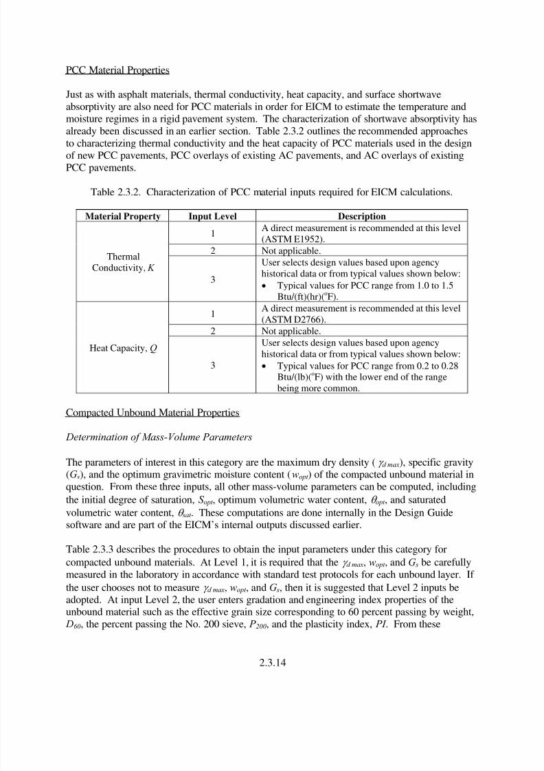
PCC Material Properties
Just as with asphalt materials, thermal conductivity, heat capacity, and surface shortwave
absorptivity are also need for PCC materials in order for EICM to estimate the temperature andmoisture regimes in a rigid pavement system. The characterization of shortwave absorptivity has
already been discussed in an earlier section. Table 2.3.2 outlines the recommended approachesto characterizing thermal conductivity and the heat capacity of PCC materials used in the designof new PCC pavements, PCC overlays of existing AC pavements, and AC overlays of existing
PCC pavements.
Table 2.3.2. Characterization of PCC material inputs required for EICM calculations.
Material Property Input Level Description
1A direct measurement is recommended at this level
(ASTM E1952).
2 Not applicable.Thermal
Conductivity, K 3
User selects design values based upon agency
historical data or from typical values shown below:
• Typical values for PCC range from 1.0 to 1.5
Btu/(ft)(hr)(oF).
1A direct measurement is recommended at this level
(ASTM D2766).
2 Not applicable.
Heat Capacity, Q
3
User selects design values based upon agency
historical data or from typical values shown below:
• Typical values for PCC range from 0.2 to 0.28Btu/(lb)(oF) with the lower end of the range
being more common.
Compacted Unbound Material Properties
Determination of Mass-Volume Parameters
The parameters of interest in this category are the maximum dry density (γ d max), specific gravity(G s), and the optimum gravimetric moisture content (wopt ) of the compacted unbound material in
question. From these three inputs, all other mass-volume parameters can be computed, including
the initial degree of saturation, S opt , optimum volumetric water content, θ opt , and saturated
volumetric water content, θ sat . These computations are done internally in the Design Guidesoftware and are part of the EICM’s internal outputs discussed earlier.
Table 2.3.3 describes the procedures to obtain the input parameters under this category for
compacted unbound materials. At Level 1, it is required that the γ d max, wopt , and G s be carefully
measured in the laboratory in accordance with standard test protocols for each unbound layer. If
the user chooses not to measure γ d max, wopt , and G s, then it is suggested that Level 2 inputs beadopted. At input Level 2, the user enters gradation and engineering index properties of theunbound material such as the effective grain size corresponding to 60 percent passing by weight,
D60, the percent passing the No. 200 sieve, P 200, and the plasticity index, PI . From these
2.3.14

8/6/2019 Chapter3 Environment Effects No Restriction
http://slidepdf.com/reader/full/chapter3-environment-effects-no-restriction 17/52
Table 2.3.3. Materials inputs required for unbound compacted material for EICM calculations—Mass-Volume Parameters.
Material Property Input Level Description
1
A direct measurement using AASHTO T100 (performed
in conjunction with consolidation tests – AASHTO T180
for bases or AASHTO T 99 for other layers).
2
Determined from P2001 and PI2 of the layer as below:
1. Determine P 200 and PI .2. Calculate G s (8):
G s = 0.041(P 200 * PI)0.29 + 2.65
Specific Gravity (oven-dry), Gs
3 Not applicable.
1
Typically, AASHTO T180 compaction test for base
layers and AASHTO T99 compaction test for other
layers.
2
Determined from D601, P200
1and PI
2of the layer as
illustrated below:
1. Read PI, P 200, and D60. Identify the layer as acompacted base course, compacted subgrade, or
natural in-situ subgrade.
2. Calculate S opt (8):
S opt = 6.752 (P 200 * PI)0.147 + 783. Compute wopt (8):
If P 200 * PI > 0
wopt = 1.3 (P 200 * PI)0.73 + 11
If P 200 * PI = 0
wopt (T99) = 8.6425 (D60 )-0.1038
If layer is not a base course
wopt = wopt (T99)
If layer is a base course∆wopt = 0.0156[wopt(T99) ]
2 – 0.1465wopt(T99) + 0.9
wopt = wopt (T99) - ∆wopt
4. To obtain G s refer to the level 2 procedure for this
input provided in this table above.
5. Compute γ d max for compacted materials, γ d max comp
6.
opt
sopt
water scompmaxd
S
Gw1
G
+
=γ
γ
7. Compute γ d max
If layer is a compacted material
compmaxmax d d γ γ =
If layer is a natural in-situ material
compmax90.0 d d γ γ =
8. EICM uses γ d for γ d max
Optimum gravimetric water
content, wopt , and maximum dry
unit weight of solids, γ dmax
3 Not applicable.1 P200 and D60 can be obtained from a grain-size distribution test (AASHTO T 27).2 PI can be determined from an Atterberg limit test (AASHTO T 90).
2.3.15
8/6/2019 Chapter3 Environment Effects No Restriction
http://slidepdf.com/reader/full/chapter3-environment-effects-no-restriction 18/52
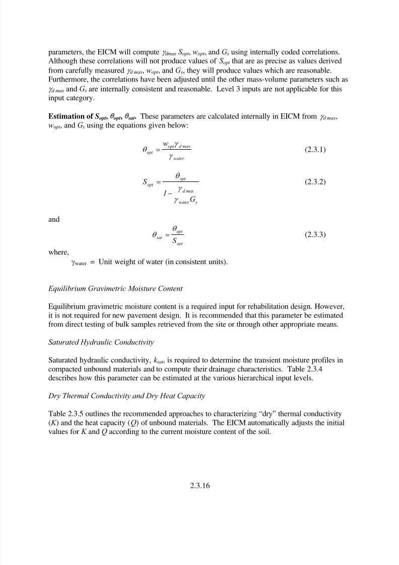
parameters, the EICM will compute γ dmax S opt , wopt , and G s using internally coded correlations.Although these correlations will not produce values of S opt that are as precise as values derived
from carefully measured γ d max, wopt , and G s, they will produce values which are reasonable.Furthermore, the correlations have been adjusted until the other mass-volume parameters such as
γ d max and G s are internally consistent and reasonable. Level 3 inputs are not applicable for this
input category.
Estimation of S opt, θ opt, θ sat. These parameters are calculated internally in EICM from γ d max,
wopt , and G s using the equations given below:
water
d opt
opt
w
γ
γ θ
max= (2.3.1)
swater
maxd
opt
opt
G1
S
γ
γ
θ
−
= (2.3.2)
and
opt
opt
sat S
θ θ = (2.3.3)
where,
γwater = Unit weight of water (in consistent units).
Equilibrium Gravimetric Moisture Content
Equilibrium gravimetric moisture content is a required input for rehabilitation design. However,it is not required for new pavement design. It is recommended that this parameter be estimated
from direct testing of bulk samples retrieved from the site or through other appropriate means.
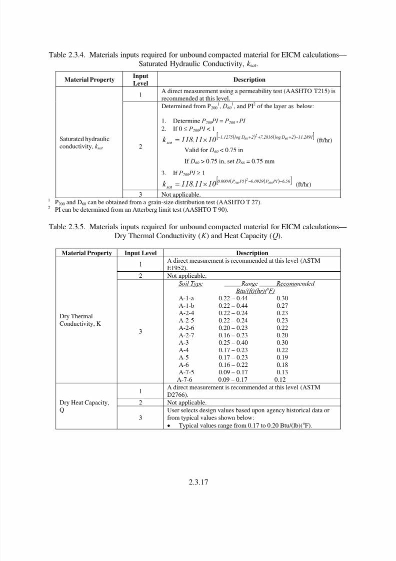
Saturated Hydraulic Conductivity
Saturated hydraulic conductivity, k sat , is required to determine the transient moisture profiles in
compacted unbound materials and to compute their drainage characteristics. Table 2.3.4describes how this parameter can be estimated at the various hierarchical input levels.
Dry Thermal Conductivity and Dry Heat Capacity
Table 2.3.5 outlines the recommended approaches to characterizing “dry” thermal conductivity
( K ) and the heat capacity (Q) of unbound materials. The EICM automatically adjusts the initialvalues for K and Q according to the current moisture content of the soil.
2.3.16
8/6/2019 Chapter3 Environment Effects No Restriction
http://slidepdf.com/reader/full/chapter3-environment-effects-no-restriction 19/52
Table 2.3.4. Materials inputs required for unbound compacted material for EICM calculations—
Saturated Hydraulic Conductivity, k sat .
Material PropertyInput
LevelDescription
1A direct measurement using a permeability test (AASHTO T215) is
recommended at this level.
2
Determined from P2001, D60
1, and PI
2of the layer as below:
1. Determine P 200 PI = P 200 * PI
2. If 0 ≤ P 200 PI < 1
( ) ( )[ ]2891.112 Dlog 2816 .7 2 Dlog 1275.1
sat 60
2601011.118k
−+++−×= (ft/hr)
Valid for D60 < 0.75 in
If D60 > 0.75 in, set D60 = 0.75 mm
3. If P 200 PI ≥ 1
( ) ( )[ ]56 .6 PI P 0929.0 PI P 0004.0
sat 200
22001011.118k
−−×= (ft/hr)
Saturated hydraulic
conductivity, k sat
3 Not applicable.1 P200 and D60 can be obtained from a grain-size distribution test (AASHTO T 27).2 PI can be determined from an Atterberg limit test (AASHTO T 90).
Table 2.3.5. Materials inputs required for unbound compacted material for EICM calculations—
Dry Thermal Conductivity ( K ) and Heat Capacity (Q).
Material Property Input Level Description
1A direct measurement is recommended at this level (ASTM
E1952).
2 Not applicable.
Dry Thermal
Conductivity, K
3
Soil Type Range Recommended Btu/(ft)(hr)( o F)
A-1-a 0.22 – 0.44 0.30
A-1-b 0.22 – 0.44 0.27
A-2-4 0.22 – 0.24 0.23
A-2-5 0.22 – 0.24 0.23
A-2-6 0.20 – 0.23 0.22
A-2-7 0.16 – 0.23 0.20
A-3 0.25 – 0.40 0.30
A-4 0.17 – 0.23 0.22
A-5 0.17 – 0.23 0.19
A-6 0.16 – 0.22 0.18
A-7-5 0.09 – 0.17 0.13
A-7-6 0.09 – 0.17 0.12
1
A direct measurement is recommended at this level (ASTM
D2766).2 Not applicable.Dry Heat Capacity,
Q
3
User selects design values based upon agency historical data or
from typical values shown below:
• Typical values range from 0.17 to 0.20 Btu/(lb)(oF).
2.3.17

8/6/2019 Chapter3 Environment Effects No Restriction
http://slidepdf.com/reader/full/chapter3-environment-effects-no-restriction 20/52
Soil Water Characteristic Curve Parameters
The SWCC defines the relationship between water content and suction for a given soil ( 15).
Table 2.3.6 outlines the recommended approach to characterizing the parameters of the SWCC ateach of the three hierarchical input levels. As part of the Design Guide development, a lot of
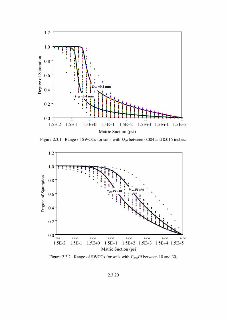
effort was expended to obtain the fitting parameters of the Fredlund and Xing equation from soilindex properties (13). As can be observed from table 2.3.6, when the soil has a PI greater thanzero, the SWCC parameters are correlated with the product of P 200 (decimal) and PI, referred to
as P 200 PI . For those cases where the PI is zero, the parameters are correlated with the D60.
Figures 2.3.1 and 2.3.2 show examples of the goodness of the fit of these correlations. The data
points shown in these figures represent the actual, measured SWCCs (after some smoothing).The goodness of the fit can be judged by observing the extent to which the "predicted" band is
centered on and envelops the experimental data. For each figure, the experimental data subset
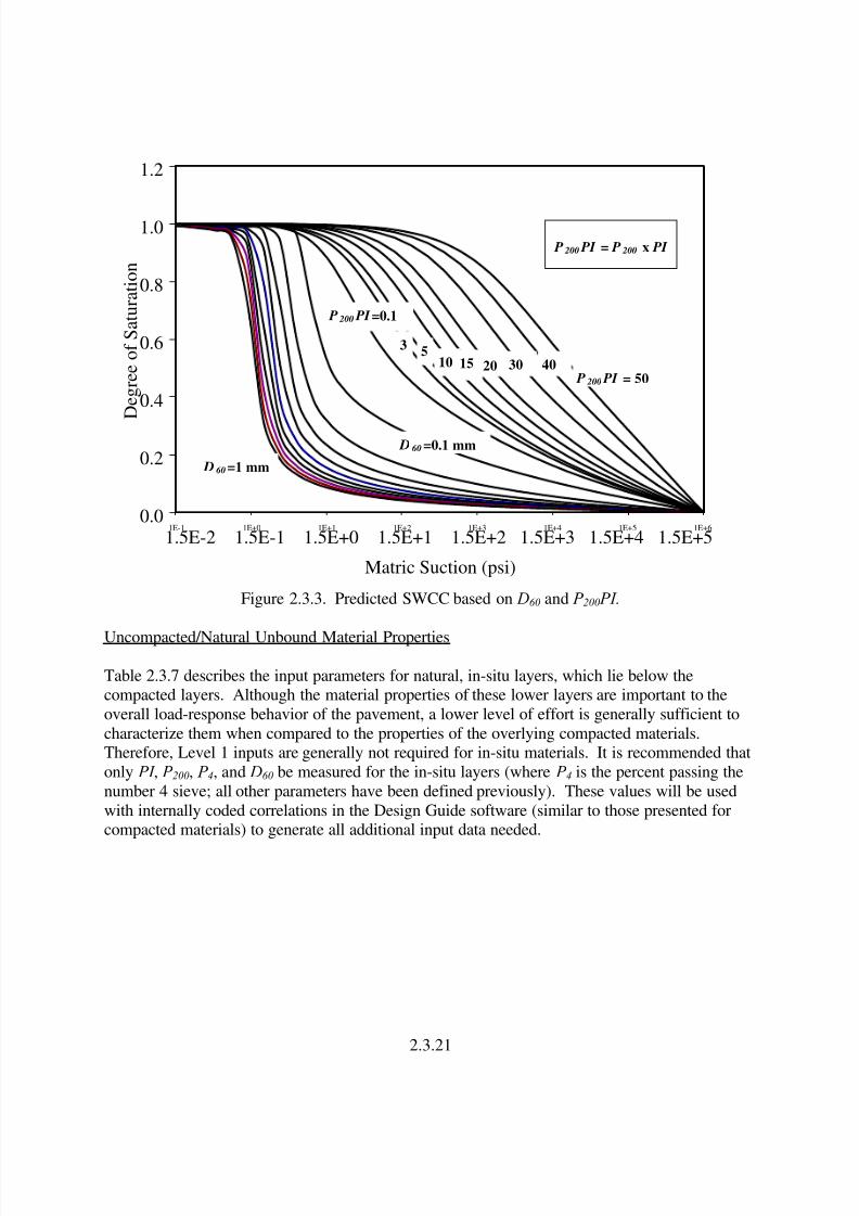
represents the same range in P 200 PI (or D60), as does the predicted band given by the solidcurves. Figure 2.3.3 summarizes the results obtained for both groups of soils.
Table 2.3.6. Options for estimating SWCC parameters.
Input
LevelProcedure to Determine SWCC Parameters Required Testing
1
1) Direct measurement of suction (h) in psi, and volumetric water
content ( θ w) pairs of values.
2) Direct measurement of optimum gravimetric water content, wopt
and maximum dry unit weight, γ d max.
3) Direct measurement of the specific gravity of the solids, G s.
4) Compute θ opt as shown in equation 2.3.1.
5) Compute the S opt as shown in equation 2.3.2.
6) Compute θ sat as shown in equation 2.3.3.
7) Based on a non-linear regression analysis, compute the SWCCmodel parameters a f , b f , c f , and hr using the equation proposed by
Fredlund and Xing, and the (h, θ w) pairs of values obtained in
step 1.
⎥⎥⎥⎥⎥⎥⎥
⎦
⎤
⎢⎢⎢⎢⎢⎢⎢
⎣
⎡
⎥⎥
⎦
⎤
⎢⎢
⎣
⎡
⎥⎥⎦
⎤
⎢⎢⎣
⎡
⎟⎟
⎠
⎞⎜⎜⎝
⎛ +
×= f c
f bw
f
sat
a
h EXP
hC
)1(ln
)(θ
θ
⎥⎥⎥⎥
⎥
⎦
⎤
⎢⎢⎢⎢
⎢
⎣
⎡
⎟⎟ ⎠
⎞⎜⎜⎝
⎛ ×+
⎟⎟
⎠
⎞⎜⎜
⎝
⎛ +
−=
r
r
h
1045.11ln
h
h1ln
1 )h( C 5
8) Input a f (psi) , b f , c f , and hr (psi) into the Design Guide
software.
9) EICM will generate the function at any water content (SWCC).
Pressure plate, filter
paper, and/or Tempe cell
testing.
AASHTO T180 or
AASHTO T99 for γ d max.AASHTO T100 for G s.
2.3.18

8/6/2019 Chapter3 Environment Effects No Restriction
http://slidepdf.com/reader/full/chapter3-environment-effects-no-restriction 21/52
Table 2.3.6. Options for estimating SWCC parameters (continued).
Input
LevelProcedure to Determine SWCC Parameters Required Testing
2
1) Direct measurement of optimum gravimetric water content, wopt
and maximum dry unit weight, γ d max.
2) Direct measurement of the specific gravity of the solids, G s.3) Direct measurement of P 200, D60, and PI .
3) The EICM will then internally do the following:
a) Calculate P 200 * PI .
b) Calculate θ opt , S opt , and θ sat as described for level 1.
c) Based on a non-linear regression analysis, the EICM will
compute the SWCC model parameters a f , b f , c f , and hr by
using correlations with P 200* PI and D60 (13).
i. If P 200 PI > 0
895.6
11 ) PI P ( 4 ) PI P ( 00364.0a 200
35.3
200
f
++= , psi
5 ) PI P ( 313.2cb 14.0
200
f
f +−=
5.0 ) PI P ( 0514.0c 465.0
200 f +=
) PI P ( 0186 .0
f
r 200e44.32a
h=
ii. If P 200 PI = 0
895.6
) D( 8627 .0a
751.0
60
f
−
= , psi
5.7= f b
7734.0)ln(1772.0 60 += Dc f
4
60 7.9
1−+
=e Da
h
f
r
d) The SWCC will then be established internally using the
Fredlund and Xing equation as shown for Level 1.
AASHTO T180 or
AASHTO T99 for γ d max.
AASHTO T100 for G s.
AASHTO T27 for P 200
and D60.
AASHTO T90 for PI .
3
Direct measurement and input of P 200 , PI , and D60, after which
EICM uses correlations with P 200 PI and D60 to automatically
generate the SWCC parameters for each soil, as follows:
1) Identify the layer as a base course or other layer
2) Compute G s as outlined in table 2.3.3 for Level 2.
3) Compute P 200 * PI 4) Compute S opt , wopt , and γ d max as shown for level 2.
6) Based on a non-linear regression analysis, the EICM will
compute the SWCC model parameters a f , b f , c f , and hr by using
correlations with P 200 PI and D60, as shown for Level 2.
7) The SWCC will then be internally established using the
Fredlund and Xing equation as shown for Level 1.
T27 for P 200 and D60.
T90 for PI .
2.3.19
8/6/2019 Chapter3 Environment Effects No Restriction
http://slidepdf.com/reader/full/chapter3-environment-effects-no-restriction 22/52
0.0
0.2
0.4
0.6
0.8
1.0
1.2
1E-1 1E+0 1E+1 1E+2 1E+3 1E+4 1E+5 1E+6
Matric Suction (psi)
D e g r e e o f S a t u r a t i o n
D 60 =0.1 mm
D 60 =0.4 mm
1.5E-2 1.5E-1 1.5E+0 1.5E+1 1.5E+2 1.5E+3 1.5E+4 1.5E+5
Figure 2.3.1. Range of SWCCs for soils with D60 between 0.004 and 0.016 inches.
0.0
0.2
0.4
0.6
0.8
1.0
1.2
1.0E-1 1.0E+0 1.0E+1 1.0E+2 1.0E+3 1.0E+4 1.0E+5 1.0E+6
Matric Suction (psi)
D e g r e e o f S a t u r a t i o n
P 200 PI =10 P 200 PI =30
1.5E-2 1.5E-1 1.5E+0 1.5E+1 1.5E+2 1.5E+3 1.5E+4 1.5E+5
Figure 2.3.2. Range of SWCCs for soils with P 200 PI between 10 and 30.
2.3.20
8/6/2019 Chapter3 Environment Effects No Restriction
http://slidepdf.com/reader/full/chapter3-environment-effects-no-restriction 23/52
0.0
0.2
0.4
0.6
0.8
1.0
1.2
1E-1 1E+0 1E+1 1E+2 1E+3 1E+4 1E+5 1E+6
Matric Suction (psi)
D e g r e e o f S a t u r a t i o n
D 60 =1 mm
P 200 PI =0.1
P 200 PI = 50
3 510 15 20 30 40
D 60 =0.1 mm
P 200 PI = P 200 x PI
1.5E-2 1.5E-1 1.5E+0 1.5E+1 1.5E+2 1.5E+3 1.5E+4 1.5E+5
Figure 2.3.3. Predicted SWCC based on D60 and P 200 PI.
Uncompacted/Natural Unbound Material Properties
Table 2.3.7 describes the input parameters for natural, in-situ layers, which lie below thecompacted layers. Although the material properties of these lower layers are important to the
overall load-response behavior of the pavement, a lower level of effort is generally sufficient to
characterize them when compared to the properties of the overlying compacted materials.Therefore, Level 1 inputs are generally not required for in-situ materials. It is recommended that
only PI , P 200, P 4, and D60 be measured for the in-situ layers (where P 4 is the percent passing the
number 4 sieve; all other parameters have been defined previously). These values will be used
with internally coded correlations in the Design Guide software (similar to those presented forcompacted materials) to generate all additional input data needed.
2.3.21

8/6/2019 Chapter3 Environment Effects No Restriction
http://slidepdf.com/reader/full/chapter3-environment-effects-no-restriction 24/52
Table 2.3.7. Inputs required for unbound natural, in-situ materials for EICM calculations.
Required Properties Options for Determination
Specific Gravity, G s
Direct measurement (Level 1) not required.
Refer to table 2.3.3 to estimate this parameter from gradation
parameters (Level 2).
Saturated Hydraulic Conductivity, k sat
Direct measurement (Level 1) not required.Refer to table 2.3.4 to estimate this parameter from gradation
parameters (Level 2).
Maximum Dry Unit Weight, γ dmax
Direct measurement (Level 1) not required.
Refer to table 2.3.3 to estimate this parameter from gradation
parameters (Level 2).
Dry Thermal Conductivity, K
Heat Capacity, Q Direct measurements or default values can be combined and
used. Refer to table 2.3.5 for a range of reasonable values.
Plasticity Index, PI Direct measurement required in accordance with AASHTO T 90.
P 200 , P 4 , D60 Direct measurement required in accordance with AASHTO T 27.
Optimum Gravimetric Water, wopt Not required. Refer to table 2.3.3.
Equilibrium Gravimetric Water
Content
Direct measurement required for rehabilitated pavement analyses.
This parameter is NOT required for new pavement design.
2.3.3 EICM CALCULATIONS – COMPOSITE ENVIRONMENTAL EFFECTS
ADJUSTMENT FACTOR, Fenv, FOR ADJUSTING MR
2.3.3.1 Relevance of Fenv to Design
To evaluate the resilient modulus of unbound materials used in the Design Guide, several factors
influencing the modulus need to be considered:
• Stress state.
• Moisture/density variations.
• Freeze/thaw effects.
The values of the resilient moduli at any location and time within a given pavement structure are
calculated as a function of the above factors.
The effect of stress state on M R of unbound layers is considered in the Design Guide approach
through the use of the universal constitutive equation that relates the resilient modulus to the
bulk stress, the octahedral shear stress, and atmospheric pressure at any given location within thepavement. In the Design Guide approach, stress-sensitivity of unbound layers is only accounted
for if the inputs are provided at Level 1 and that too only for flexible pavement design. In the
Design Guide software execution, the FEA module is used for structural computations in placeof the LEA module when Level 1modulus inputs are provided for unbound materials. At input
Levels 2 and 3, stress sensitivity is not considered. At Level 2, the user enters an estimate of M R
at a reference moisture condition which is determined at or near the optimum moisture contentand maximum dry density. At this input level, it is also possible to enter other parameters such
as CBR, R-values, structural layer coefficient (ai), and so on at a reference moisture condition
from which an estimate of M R can be obtained using standard correlations. At input Level 3, an
2.3.22

8/6/2019 Chapter3 Environment Effects No Restriction
http://slidepdf.com/reader/full/chapter3-environment-effects-no-restriction 25/52
estimate of the M R is sufficient. More details on the configuring the resilient modulus input for
unbound materials can be obtained in PART 2, Chapter 2.
Although the stress sensitivity is only considered if Level 1 inputs are used, the impact of
temporal variations in moisture and temperature on M R are fully considered at all levels through
the composite environmental adjustment factor, F env. The EICM deals with all environmentalfactors and provides soil moisture, suction, and temperature as a function of time, at any locationin the unbound layers from which F env can be determined. The resilient modulus M R at any time
or position is then expressed as follows:
Ropt env R M F M ⋅=(2.3.4)
The factor F env is an adjustment factor and M Ropt is the resilient modulus at optimum conditions
(maximum dry density and optimum moisture content) and at any state of stress. It is obvious inequation 2.3.4 that the variation of the modulus with stress and the variation of the modulus with
environmental factors (moisture, density, and freeze/thaw conditions) are assumed independent.
Although this is not necessarily the case, recent studies support the use of this assumption inpredicting resilient modulus without significant loss in accuracy of prediction. The adjustment
factor F env, being solely a function of the environmental factors, can then be computed inside the
EICM, without actually knowing M Ropt .
2.3.3.2 Environmental Effects on M R of Unbound Pavement Materials
As has been stated earlier in this chapter, in a pavement structure, moisture and temperature are
the two environmentally driven variables that can significantly affect the resilient modulus of
unbound materials.
All other conditions being equal, the higher the moisture content the lower the modulus;however, moisture has two separate effects:
•
•
o It can affect the state of stress, through suction or pore water pressure.
o It can affect the structure of the soil, through destruction of the cementation betweensoil particles (16).
At freezing temperatures, water in soil freezes and the resilient modulus rises to values 20to 120 times higher than the value of the modulus before freezing; the process may be
accompanied by the formation of ice lenses that create zones of greatly reduced strengthin the pavement when thawing occurs.
The development of predictive equations and techniques that address the influence of changes inmoisture and freeze/thaw cycles on the resilient modulus of unbound materials is described in thefollowing two subsections.
Resilient Modulus as Function of Soil Moisture
An intensive literature review study was completed with the objective of summarizing existing
models that incorporated the variation of resilient modulus with moisture (5). Using these
2.3.23

8/6/2019 Chapter3 Environment Effects No Restriction
http://slidepdf.com/reader/full/chapter3-environment-effects-no-restriction 26/52
published models from the literature (17 , 18, 19, 20), it was possible to develop (select) a model
that would analytically predict changes in modulus due to changes in moisture. This model is
presented in equation 2.3.5.
( )⎟ ⎠ ⎞⎜
⎝ ⎛ −⋅+−+
−
+=opt m
Ropt
R
S S k a
bln EXP 1
ab
aM
M
log (2.3.5)
where,
M R / M Ropt = Resilient modulus ratio; M R is the resilient modulus at a given time and
M Ropt is the resilient modulus at a reference condition. a = Minimum of log(M R /M Ropt ).
b = Maximum of log(M R /M Ropt ).
k m = Regression parameter.
(S – S opt ) = Variation in degree of saturation expressed in decimal.
Equation 2.3.5 approaches a linear form for degrees of saturation, S , within +/- 30% of S opt butflattens out for degrees of saturation lower than 30% below the optimum. This extrapolation is
in general agreement with known behavior of unsaturated materials in that, when a materialbecomes sufficiently dry, further drying increments produce less increase in stiffness and
strength (21).
Using the available literature data and adopting a maximum modulus ratio of 2.5 for fine-grained
materials and 2 for coarse-grained materials, the values of a, b, and k m for coarse-grained andfine-grained materials are given in table 2.3.8. The predictions of this revised model are shown
in figures 2.3.4 and 2.3.5, for fine-grained and coarse-grained materials, on semi-log scales. This
model is implemented within the EICM version linked to the Design Guide software.
Table 2.3.8. Values of a, b, and k m for coarse-grained and fine-grained materials.
ParameterCoarse-Grained
Materials
Fine-Grained
MaterialsComments
a - 0.3123 -0.5934 Regression parameter.
b 0.3 0.4
Conservatively assumed, corresponding
to modulus ratios of 2 and 2.5,
respectively.
k m 6.8157 6.1324 Regression parameter.
2.3.24

8/6/2019 Chapter3 Environment Effects No Restriction
http://slidepdf.com/reader/full/chapter3-environment-effects-no-restriction 27/52
Fine-grained Materials
-0.6
-0.5
-0.4
-0.3
-0.2
-0.1
0.0
0.1
0.2
0.3
0.4
0.5
0.6
-75 -70 -65 -60 -55 -50 -45 -40 -35 -30 -25 -20 -15 -10 -5 0 5 10 15 20 25 30
(S - Sopt)%
l o g M R / M R o p t
Literature Data
Predicted
Figure 2.3.4. Resilient modulus - moisture model for fine-grained materials
(semi-log scale).
Coarse-grained Materials
-0.6
-0.5
-0.4
-0.3
-0.2
-0.1
0.0
0.1
0.2
0.3
0.4
0.5
0.6
-75 -70 -65 -60 -55 -50 -45 -40 -35 -30 -25 -20 -15 -10 -5 0 5 10 15 20 25 30
(S - Sopt)%
l o g M R / M R o p t
Literature Data
Predicted
Figure 2.3.5. Resilient modulus - moisture model for coarse-grained materials
(semi-log scale).
2.3.25

8/6/2019 Chapter3 Environment Effects No Restriction
http://slidepdf.com/reader/full/chapter3-environment-effects-no-restriction 28/52
The Choice of Optimum Conditions as the Reference and Initial Conditions for M R
As stated in PART 2, Chapter 2 and throughout this chapter, the required user input for stiffnessof unbound materials is the M R value estimated at or near optimum moisture and maximum dry
density. The purpose of this section is to present the rationale behind the choice of optimum as
the reference condition for the evaluation of M R and as the initial condition for compactedunbound layers for input to the Design Guide software. The reference condition will beconsidered first.
• From literature it was found that the majority of resilient modulus tests have been
performed on specimens at optimum conditions (γ d = γ dmax, w = wopt and S = S opt ) than anyother condition (6). Therefore, if optimum is made the reference condition, the database
for the M Ropt value will grow rapidly and the ability to make reasonable estimates of M Ropt without resilient modulus testing will grow with it.
• It is common practice to require that contractors compact bases to at least 95% of γ dmax by
T180 (Modified) and other layers to 95% of γ dmax by T99 (Standard). Given that
contractors will typically target compaction somewhat above the minimum required, fieldcompaction of γ d = γ dmax is a reasonable approximation used in the Design Guide as the
reference condition. Moisture content is rarely controlled strictly by specification, butgood construction practice will force contractors to wet the material near optimum to
facilitate compaction. Thus w = wopt and S = S opt are also reasonable assumptions for
reference conditions, although the actual moisture content for field compaction may varyfrom somewhat higher to somewhat lower than optimum.
The choice of optimum as both reference condition and initial condition is both reasonable andpractical. The actual compaction density and moisture can of course be measured at several
specific points in the pavement structure, but not before construction. However, design of the
pavement is performed well before construction. Furthermore, even if the precise γ d and w wereknown at the design stage, the probability of having a database of M R values at this condition is
not high.
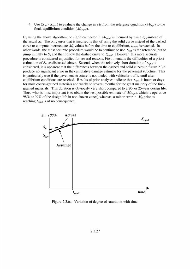
The implications of the choice of optimum as reference and initial condition can be examined by
discussing figure 2.3.6. If compaction at S opt is assumed, then it is likewise assumed that S changes (increases or decreases) to an equilibrium value, S equil with time as shown by the solidcurve in figure 2.3.6a or in figure 2.3.6b. In either case, S equil is computed by the EICM, using
the given depth to the groundwater table, yGWT , and the soil-water characteristic curve, SWCC.
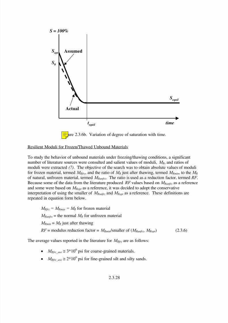
Thus the value of S equil does not actually depend on the initial S . If the actual initial degree of saturation, S 0, is slightly higher than S opt as shown in figure 2.3.6a or slightly lower than S opt as
shown in figure 2.3.6b, the dashed path is followed to S equil . Given that optimum has been chosenas the reference condition, it is the change from S opt to S equil that is of primary interest. The
process of making a best estimate of the M R under equilibrium conditions is as follows:
1. Estimate or measure M R at optimum conditions to get M Ropt .
2. Estimate or measure S opt .3. Use the EICM to compute S equil .
2.3.26
8/6/2019 Chapter3 Environment Effects No Restriction
http://slidepdf.com/reader/full/chapter3-environment-effects-no-restriction 29/52
4. Use (S opt - S equil ) to evaluate the change in M R from the reference condition (M Ropt ) to the
final, equilibrium condition (M Requil ).
By using the above algorithm, no significant error in M Requil is incurred by using S opt instead of
the actual S 0. The only error that is incurred is that of using the solid curve instead of the dashed
curve to compute intermediate M R values before the time to equilibrium, t equil , is reached. Inother words, the most accurate procedure would be to continue to use S opt as the reference, but to jump initially to S 0 and then follow the dashed curve to S equil . However, this more accurate
procedure is considered unjustified for several reasons. First, it entails the difficulties of a priori
estimation of S 0, as discussed above. Second, when the relatively short duration of t equil isconsidered, it is apparent that the differences between the dashed and solid curves in figure 2.3.6
produce no significant error in the cumulative damage estimate for the pavement structure. This
is particularly true if the pavement structure is not loaded with vehicular traffic until afterequilibrium conditions are reached. Results of prior analyses indicate that t equil is hours or days
for most coarse-grained materials and weeks to several months for the great majority of the fine-
grained materials. This duration is obviously very short compared to a 20- or 25-year design life.
Thus, what is most important is to obtain the best possible estimate of M Requil , which is operative98% or 99% of the design life in non-frozen zones) whereas, a minor error in M R prior to
reaching t equil is of no consequence.
S = 100%
time tequil
S opt
S0
Sequil
Assumed
Actual
Figure 2.3.6a. Variation of degree of saturation with time.
2.3.27
8/6/2019 Chapter3 Environment Effects No Restriction
http://slidepdf.com/reader/full/chapter3-environment-effects-no-restriction 30/52
S = 100%
time tequil
S opt
S0
Sequil
Assumed
Actual
Figure 2.3.6b. Variation of degree of saturation with time.
Resilient Moduli for Frozen/Thawed Unbound Materials
To study the behavior of unbound materials under freezing/thawing conditions, a significantnumber of literature sources were consulted and salient values of moduli, M R, and ratios of
moduli were extracted (7). The objective of the search was to obtain absolute values of moduli
for frozen material, termed M Rfrz , and the ratio of M R just after thawing, termed M Rmin, to the M R of natural, unfrozen material, termed M Runfrz . The ratio is used as a reduction factor, termed RF .Because some of the data from the literature produced RF values based on M Runfrz as a reference
and some were based on M Ropt as a reference, it was decided to adopt the conservativeinterpretation of using the smaller of M Runfrz and M Ropt as a reference. These definitions are
repeated in equation form below.
M Rfrz = M Rmax = M R for frozen material
M Runfrz = the normal M R for unfrozen material
M Rmin = M R just after thawing
RF = modulus reduction factor = M Rmin /smaller of (M Runfrz , M Ropt ) (2.3.6)
The average values reported in the literature for M Rfrz are as follows:
• M Rfrz_ave ≅ 3*106 psi for coarse-grained materials.
• M Rfrz_ave ≅ 2*106 psi for fine-grained silt and silty sands.
2.3.28

8/6/2019 Chapter3 Environment Effects No Restriction
http://slidepdf.com/reader/full/chapter3-environment-effects-no-restriction 31/52
• M Rfrz_ave ≅ 1*106 psi for clays.
If a single value were selected for all frozen soils, 2*10 6 psi would be a reasonably unbiased
estimate and 1*106 psi would be a conservative estimate.
For thawed materials, the degree of M R degradation upon thawing was found to be correlatedwith frost-susceptibility, or the ability of the soil to sustain ice lens formation under favorable
conditions. Frost-susceptibility in turn can be estimated from the percent passing the No. 200
sieve, P 200, and the Plasticity Index, PI . In tables 2.3.9 and 2.3.10, RF values used in the DesignGuide approach are given for coarse-grained and fine-grained materials as a function of P 200 and
PI .
Table 2.3.9. Recommended values of RF for coarse-grained materials ( P 200 < 50%).
Distribution of
Coarse Fraction* P 200 (%) PI < 12% PI = 12% - 35% PI > 35%
< 6 0.85 - -
6 – 12 0.65 0.70 0.75Mostly Gravel P 4 < 50% > 12 0.60 0.65 0.70
< 6 0.75 - -
6 – 12 0.60 0.65 0.70Mostly Sand
P 4 > 50% > 12 0.50 0.55 0.60
* If it is unknown whether a coarse-grained material is mostly gravel or mostly sand, assume sand.
Table 2.3.10. Recommended values of RF for fine-grained materials ( P 200 > 50%).
P 200 (%) PI < 12% PI = 12% - 35% PI > 35%
50 - 85 0.45 0.55 0.60
> 85 0.40 0.50 0.55
Recovering materials experience a rise in modulus with time, from M Rmin to M Runfrz , that can be
tracked using a recovery ratio ( RR) that ranges from 0 to 1:
• RR = 0 for the "immediately after thawing" condition, when excess water makes thesuction go to zero, M Rrecov = M Rmin.
• RR = 1 when the suction is equal to the suction dictated by the depth to the ground watertable – i.e., equilibrium is achieved, M Rrecov = M Runfrz .
RT
t RR
∆= (2.3.7)
where,
RR = Recovery ratio.
∆ t = Number of hours elapsed since thawing started.
T R = Recovery period: Number of hours required for the
material to recover from the thawed condition to thenormal, unfrozen condition.
2.3.29
8/6/2019 Chapter3 Environment Effects No Restriction
http://slidepdf.com/reader/full/chapter3-environment-effects-no-restriction 32/52
For the Design Guide, the recovery period, T R, is noted as a function of the material
type/properties, as follows:
• T R = 90 days for sands/gravels with P 200 PI < 0.1.
• T R = 120 days for silts/clays with 0.1 < P 200 PI < 10.
• T R = 150 days for clays with P 200 PI > 10.
In the ensuing section, the algorithm used in the Design Guide that outlines a methodology for
obtaining the composite moduli for layers in which two or more states of the material coexist
and/or the resilient modulus varies with depth and time is presented.
2.3.3.3 Computation of Environmental Adjustment Factor, Fenv
The resilient modulus M R at any time or position is determined as a product of the composite
environmental adjustment factor, F env, and the resilient modulus at optimum conditions M Ropt
(see equation 2.3.4). The computation of the F env as a function of all the Design Guide inputs
and EICM estimated parameters discussed so far will be presented in this section.
The environmental adjustment factor, F env is a composite factor, which could in general represent
a weighted average of the factors appropriate for various possible conditions:
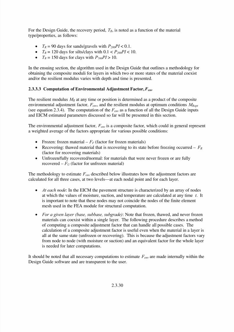
• Frozen: frozen material – F F (factor for frozen materials)
• Recovering: thawed material that is recovering to its state before freezing occurred – F R
(factor for recovering materials)
• Unfrozen/fully recovered/normal: for materials that were never frozen or are fully
recovered – F U (factor for unfrozen material)
The methodology to estimate F env described below illustrates how the adjustment factors arecalculated for all three cases, at two levels—at each nodal point and for each layer.
• At each node: In the EICM the pavement structure is characterized by an array of nodesat which the values of moisture, suction, and temperature are calculated at any time t . It
is important to note that these nodes may not coincide the nodes of the finite element
mesh used in the FEA module for structural computation.
• For a given layer (base, subbase, subgrade): Note that frozen, thawed, and never frozenmaterials can coexist within a single layer. The following procedure describes a method
of computing a composite adjustment factor that can handle all possible cases. Thecalculation of a composite adjustment factor is useful even when the material in a layer is
all at the same state (unfrozen or recovering). This is because the adjustment factors vary
from node to node (with moisture or suction) and an equivalent factor for the whole layeris needed for later computations.
It should be noted that all necessary computations to estimate F env are made internally within theDesign Guide software and are transparent to the user.
2.3.30

8/6/2019 Chapter3 Environment Effects No Restriction
http://slidepdf.com/reader/full/chapter3-environment-effects-no-restriction 33/52
Adjustment Factors at Node Level
The computation of the adjustment factors for each specific case (frozen, recovering, unfrozen)at the node level follows:
F F – Adjustment Factor for Frozen Materials
The value of F F is computed at each node at which a freezing temperature occurs. Table 2.3.11
presents the procedure in the Design Guide to estimate this parameter.
Table 2.3.11. Summary of computations made by the EICM to determine adjustment factor for
frozen material, F F .
Step No. Description
1 From user entered P 200 , PI , and D60, compute P 200 * PI .
2
Obtain an estimated value of M Ropt_est (user input).
M Ropt is either a direct user input or can be estimated from other engineeringproperties such as CBR, R-value, structural layer coefficients (ai ), PenetrationIndex, or from gradation parameters as explained in PART 2, Chapter 2.
3
Assign values for the Frozen Resilient Modulus, M R frz (7):a) If P 200* PI = 0
M R frz = 2.5 X 10⁶
psib) If P 200* PI > 0
M R frz = 1 X 10⁶
psi
4
Compute the frozen adjustment factor, F F (7):
opt_est R
frz R
F M
M F =
F R – Adjustment Factor for Recovering Materials
The value of F R is computed at each node at which freezing temperatures do not occur and the
recovery ratio RR is < 1. Table 2.3.12 presents the procedure implemented in the Design Guide
software to estimate this parameter.
F U – Adjustment Factor for Unfrozen or Fully Recovered Materials
Table 2.3.13 presents the procedure implemented in the Design Guide software to estimate F U .
2.3.31

8/6/2019 Chapter3 Environment Effects No Restriction
http://slidepdf.com/reader/full/chapter3-environment-effects-no-restriction 34/52
Table 2.3.12. Summary of computations made by the EICM to determine adjustment factor for
recovering material, F F .
Step No. Description
1Obtain user input gradation parameters P 200 , P 4 , PI , and D60 as well as
estimated depth to water table, yGWT . Compute P 200 * PI .
2
Compute Recovery Ratio, RR:
RT
t RR
∆=
where,
∆t = number of hours elapsed since thawing started
T R, the recovery period, is a function of the material properties:
- T R = 90 days for sands/gravels with P 200 * PI < 0.1;
- T R = 120 days for silts/clays with 0.1 < P 200 * PI < 10; and,
- T R = 150 days for clays with P 200 * PI > 10.
3
Compute S opt as discussed in table 2.3.3 for Level 2 or as in equation 2.3.2 for
Level 1.
4
Compute S equil from the SWCC (9) :
f c f b
equil
f a
h EXP
hC S
⎥⎥
⎦
⎤
⎢⎢
⎣
⎡
⎥⎥⎦
⎤
⎢⎢⎣
⎡
⎟⎟
⎠
⎞⎜⎜⎝
⎛ +
×=
)1(ln
1)(
⎟⎟ ⎠
⎞⎜⎜⎝
⎛ ×+
⎟⎟ ⎠
⎞⎜⎜⎝
⎛ +
−=
r
r
h
1045.11ln
h
h1ln
1 )h( C 5
where: h = yGWT * γ water , in psi
a f (psi) , b f , c f , and hr (psi) are calculated as in table 2.3.6.
5
Compute Requil value as (5) :
( )⎥⎦
⎤⎢⎣
⎡−+⎟
⎠
⎞⎜⎝
⎛ −+
−+==
opt equil m
Ropt
quil Re
equil
S S k a
bln EXP 1
aba
M
M log Rlog
where: a, b, and k m are constants from table 2.3.8.
6Compute the RF value as a function of PI, P 4, and P 200 from tables 2.3.9 and
2.3.10.
7
Compute the factor for recovering material, F R (7):
If (S equil – S opt ) < 0:
F R = RF + Requi l * RR – RR * RF If (S equil – S opt ) > 0:
F R = Requil (RF + RR – RR * RF)
2.3.32

8/6/2019 Chapter3 Environment Effects No Restriction
http://slidepdf.com/reader/full/chapter3-environment-effects-no-restriction 35/52
Table 2.3.13. Summary of computations made by the EICM to determine adjustment factor for
unfrozen or fully recovered material, F U .
Step No. Description
1Compute S opt as discussed in table 2.3.3 for Level 2 or as in equation 2.3.2 for
Level 1.
2
Compute the adjustment factor for unfrozen or fully recovered material, F U
(5):
( )⎥⎦
⎤⎢⎣
⎡−+⎟
⎠
⎞⎜⎝
⎛ −+
−+==
opt m
Ropt
RU
S S k a
bln EXP 1
aba
M
M log F log
where: a, b, and k m are constants from table 2.3.8.
S is the estimated degree of saturation at any node.
Composite Adjustment Factors, F env, for Structural Layers To help visualize possible changes in M R caused by changes in the physical state with time, a
time–depth diagram for a typical pavement structure is presented in figure 2.3.7. The three
possible states of the material are identified: frozen (dark gray, denoted F F ), recovering (light
gray, denoted F R) and unfrozen or fully recovered (white, denoted F U ).
The solution to the problem of generating a composite adjustment factor, F env, consists of
building a matrix that will have as elements M R adjustment factors at node i at time t , having thenumber of rows equal to the number of nodes and the number of columns equal to the number of
time increments (one hour for each time increment) considered in the analysis period (2-week
period or 1 month). The matrix corresponding to the time–depth diagram is shown in figure2.3.8. The elements of the matrix are shown as F F , F R and F U depending on the state of the
material. In figure 2.3.8, example numerical values of F F , F R, and F U are evaluated at each
node/time and symbols are replaced with numbers.
Once the matrix of adjustment factors is established, it is subdivided as follows:
(a) In layers, corresponding to the structural layers (base, subbase, subgrade) defined by theuser.
(b) In sublayers, defined by the EICM as needed by the subsequent modules. This
sublayering is also a function of the frost penetration depth.(c) For each analysis period (2 weeks or 1 month), a "sub-matrix" of M R adjustment factors is
assigned to each sublayer.
If the elements of the matrices were modulus values, corresponding to a temporary assumption
that M Ropt = 1, then a simple way to obtain an equivalent modulus is to consider an elastic spring
series analogy. Consider the elements of column 1 (corresponding to Hour 1, for example) of a
node/time matrix, as elastic moduli of a series of springs (one spring per node). If the stress
2.3.33
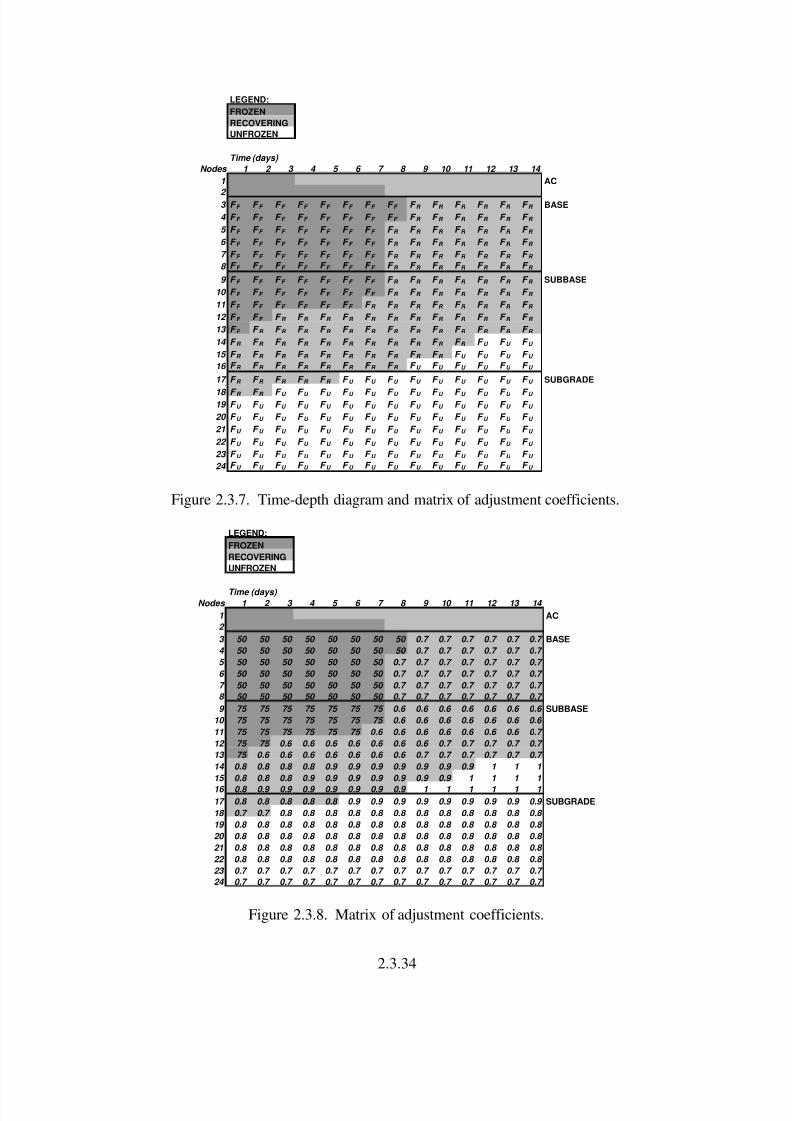
8/6/2019 Chapter3 Environment Effects No Restriction
http://slidepdf.com/reader/full/chapter3-environment-effects-no-restriction 36/52
LEGEND:
FROZEN
RECOVERING
UNFROZEN
Time (days)
Nodes 1 2 3 4 5 6 7 8 9 10 11 12 13 14
1 AC
2 3 F F F F F F F F F F F F F F F F F R F R F R F R F R F R BASE
4 F F F F F F F F F F F F F F F F F R F R F R F R F R F R
5 F F F F F F F F F F F F F F F R F R F R F R F R F R F R
6 F F F F F F F F F F F F F F F R F R F R F R F R F R F R
7 F F F F F F F F F F F F F F F R F R F R F R F R F R F R
8 F F F F F F F F F F F F F F F R F R F R F R F R F R F R
9 F F F F F F F F F F F F F F F R F R F R F R F R F R F R SUBBASE
10 F F F F F F F F F F F F F F F R F R F R F R F R F R F R
11 F F F F F F F F F F F F F R F R F R F R F R F R F R F R
12 F F F F F R F R F R F R F R F R F R F R F R F R F R F R
13 F F F R F R F R F R F R F R F R F R F R F R F R F R F R
14 F R F R F R F R F R F R F R F R F R F R F R F U F U F U
15 F R F R F R F R F R F R F R F R F R F R F U F U F U F U
16 F R F R F R F R F R F R F R F R F U F U F U F U F U F U
17 F R F R F R F R F R F U F U F U F U F U F U F U F U F U SUBGRADE
18 F R F R F U F U F U F U F U F U F U F U F U F U F U F U
19 F U F U F U F U F U F U F U F U F U F U F U F U F U F U
20 F U F U F U F U F U F U F U F U F U F U F U F U F U F U
21 F U F U F U F U F U F U F U F U F U F U F U F U F U F U
22 F U F U F U F U F U F U F U F U F U F U F U F U F U F U
23 F U F U F U F U F U F U F U F U F U F U F U F U F U F U
24 F U F U F U F U F U F U F U F U F U F U F U F U F U F U
Figure 2.3.7. Time-depth diagram and matrix of adjustment coefficients.
LEGEND:
FROZEN
RECOVERING
UNFROZEN
Time (days)
Nodes 1 2 3 4 5 6 7 8 9 10 11 12 13 14
1 AC
2
3 50 50 50 50 50 50 50 50 0.7 0.7 0.7 0.7 0.7 0.7 BASE
4 50 50 50 50 50 50 50 50 0.7 0.7 0.7 0.7 0.7 0.7
5 50 50 50 50 50 50 50 0.7 0.7 0.7 0.7 0.7 0.7 0.7
6 50 50 50 50 50 50 50 0.7 0.7 0.7 0.7 0.7 0.7 0.7
7 50 50 50 50 50 50 50 0.7 0.7 0.7 0.7 0.7 0.7 0.7
8 50 50 50 50 50 50 50 0.7 0.7 0.7 0.7 0.7 0.7 0.7
9 75 75 75 75 75 75 75 0.6 0.6 0.6 0.6 0.6 0.6 0.6 SUBBASE
10 75 75 75 75 75 75 75 0.6 0.6 0.6 0.6 0.6 0.6 0.6
11 75 75 75 75 75 75 0.6 0.6 0.6 0.6 0.6 0.6 0.6 0.7
12 75 75 0.6 0.6 0.6 0.6 0.6 0.6 0.6 0.7 0.7 0.7 0.7 0.7
13 75 0.6 0.6 0.6 0.6 0.6 0.6 0.6 0.7 0.7 0.7 0.7 0.7 0.7
14 0.8 0.8 0.8 0.8 0.9 0.9 0.9 0.9 0.9 0.9 0.9 1 1 1
15 0.8 0.8 0.8 0.9 0.9 0.9 0.9 0.9 0.9 0.9 1 1 1 1
16 0.8 0.9 0.9 0.9 0.9 0.9 0.9 0.9 1 1 1 1 1 1
17 0.8 0.8 0.8 0.8 0.8 0.9 0.9 0.9 0.9 0.9 0.9 0.9 0.9 0.9 SUBGRADE
18 0.7 0.7 0.8 0.8 0.8 0.8 0.8 0.8 0.8 0.8 0.8 0.8 0.8 0.8
19 0.8 0.8 0.8 0.8 0.8 0.8 0.8 0.8 0.8 0.8 0.8 0.8 0.8 0.8
20 0.8 0.8 0.8 0.8 0.8 0.8 0.8 0.8 0.8 0.8 0.8 0.8 0.8 0.8
21 0.8 0.8 0.8 0.8 0.8 0.8 0.8 0.8 0.8 0.8 0.8 0.8 0.8 0.8
22 0.8 0.8 0.8 0.8 0.8 0.8 0.8 0.8 0.8 0.8 0.8 0.8 0.8 0.8
23 0.7 0.7 0.7 0.7 0.7 0.7 0.7 0.7 0.7 0.7 0.7 0.7 0.7 0.7
24 0.7 0.7 0.7 0.7 0.7 0.7 0.7 0.7 0.7 0.7 0.7 0.7 0.7 0.7
Figure 2.3.8. Matrix of adjustment coefficients.
2.3.34

8/6/2019 Chapter3 Environment Effects No Restriction
http://slidepdf.com/reader/full/chapter3-environment-effects-no-restriction 37/52
applied to this model is σ , then the displacement in one spring at a given node and time
increment can be computed as:
t node R
nodet node
M
h
,
,
⋅=σ
δ
(2.3.8)
where,
node = Node number.
t = Time (corresponding to the column in the matrix being considered).
hnode = Length of the spring assigned to the node being considered.
M Rnode,t = Modulus for the node.
The total displacement for the given time is given by the sum of displacements from all nodes atthe considered time t , which is a summation vertically, for example, for Hour 1:
∑== ⋅=
n
node node R
nodet
M h
1
1 σ δ (2.3.9)
where,
n = Number of nodes (rows in the matrix).
To get the average displacement over the whole analysis period (2 weeks or 1 month), equation
2.3.10 is used:
∑ ∑= = ⎟
⎟
⎠
⎞
⎜
⎜
⎝
⎛
⎟⎟
⎠
⎞⎜⎜
⎝
⎛ ⋅⋅=
total t
t
n
node t node R
node
total
average
M
h
t 1 1 ,
1σ δ
(2.3.10)
where:
t total = Total number of t time increments over which the composite modulus iscalculated (number of columns in the matrix). For use in the EICM,
each time increment has been set to 1 hour.
Then the composite (equivalent) modulus can be obtained by finding a composite modulus,
M Rcomp, which produces the same δ average over the total layer thickness for the same applied σ .
Equating δ average for the composite model to δ average from equation 2.3.10 and canceling σ which
appears on both sides:
∑ ∑= =
⎟⎟
⎠
⎞
⎜⎜
⎝
⎛
⎟⎟
⎠
⎞
⎜⎜
⎝
⎛ ⋅=
total
t node
t
t
n
node R
node
total Rcomp
total
M
h
t M
h
1 1,
1
(2.3.11)where,
htotal = Total height of the considered layer/sublayer, and:
2.3.35

8/6/2019 Chapter3 Environment Effects No Restriction
http://slidepdf.com/reader/full/chapter3-environment-effects-no-restriction 38/52
∑=
=n
node
nodetotal hh1 (2.3.12)
Because the resilient modulus at any node/time can be expressed as the product of an adjustment
factor times the resilient modulus at optimum, equation 2.3.11 can be replaced with equation2.3.13. A composite adjustment factor, F env , for the considered sub-layer (sub-matrix) can be
obtained from:
∑ ∑
∑ ∑
= =
= =
⎟⎟ ⎠
⎞⎜⎜⎝
⎛ ⎟⎟ ⎠
⎞⎜⎜⎝
⎛
⋅=
⎟⎟
⎠
⎞
⎜⎜
⎝
⎛ ⎟⎟ ⎠
⎞⎜⎜⎝
⎛
⋅⋅=
⋅
total
total
t
t
n
node t node
node
total total env
t
t
n
node Ropt t node
node
total Ropt env
total
F
h
t h F
M F
h
t M F
h
1 1 ,
1 1 ,
1
(2.3.13)
where, F env = Composite adjustment factor for the considered sublayer.
F node,t = Adjustment factor at a given node and time increment (which could be F F , F R, or
F U , depending on the state of the material).
As an example, F env is computed for the subbase and the subgrade layers in figure 2.3.9. Forsimplification, equal lengths are assigned to each node.
LEGEND:
FROZEN
RECOVERING
UNFROZEN
Time (days)
Nodes 1 2 3 4 5 6 7 8 9 10 11 12 13 14
3 50 50 50 50 50 50 50 50 0.7 0.7 0.7 0.7 0.7 0.7 BASE
4 50 50 50 50 50 50 50 50 0.7 0.7 0.7 0.7 0.7 0.7 F env = 1.45
5 50 50 50 50 50 50 50 0.7 0.7 0.7 0.7 0.7 0.7 0.7
6 50 50 50 50 50 50 50 0.7 0.7 0.7 0.7 0.7 0.7 0.7
7 50 50 50 50 50 50 50 0.7 0.7 0.7 0.7 0.7 0.7 0.7
8 50 50 50 50 50 50 50 0.7 0.7 0.7 0.7 0.7 0.7 0.7
9 75 75 75 75 75 75 75 0.6 0.6 0.6 0.6 0.6 0.6 0.6 SUBBASE
10 75 75 75 75 75 75 75 0.6 0.6 0.6 0.6 0.6 0.6 0.6 F env = 0.9211 75 75 75 75 75 75 0.6 0.6 0.6 0.6 0.6 0.6 0.6 0.7
12 75 75 0.6 0.6 0.6 0.6 0.6 0.6 0.6 0.7 0.7 0.7 0.7 0.7
13 75 0.6 0.6 0.6 0.6 0.6 0.6 0.6 0.7 0.7 0.7 0.7 0.7 0.7
14 0.8 0.8 0.8 0.8 0.9 0.9 0.9 0.9 0.9 0.9 0.9 1 1 1
15 0.8 0.8 0.8 0.9 0.9 0.9 0.9 0.9 0.9 0.9 1 1 1 1
16 0.8 0.9 0.9 0.9 0.9 0.9 0.9 0.9 1 1 1 1 1 1
Figure 2.3.9. Example computations of F env.
2.3.36
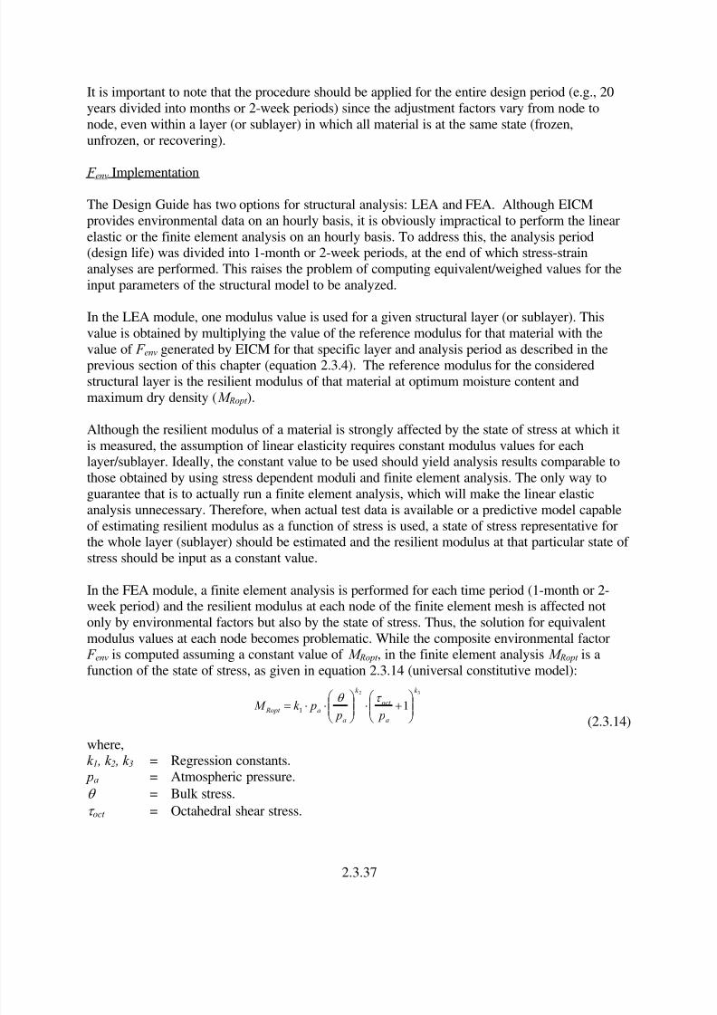
8/6/2019 Chapter3 Environment Effects No Restriction
http://slidepdf.com/reader/full/chapter3-environment-effects-no-restriction 39/52
It is important to note that the procedure should be applied for the entire design period (e.g., 20
years divided into months or 2-week periods) since the adjustment factors vary from node to
node, even within a layer (or sublayer) in which all material is at the same state (frozen,
unfrozen, or recovering).
F env Implementation
The Design Guide has two options for structural analysis: LEA and FEA. Although EICM
provides environmental data on an hourly basis, it is obviously impractical to perform the linear
elastic or the finite element analysis on an hourly basis. To address this, the analysis period(design life) was divided into 1-month or 2-week periods, at the end of which stress-strain
analyses are performed. This raises the problem of computing equivalent/weighed values for the
input parameters of the structural model to be analyzed.
In the LEA module, one modulus value is used for a given structural layer (or sublayer). This
value is obtained by multiplying the value of the reference modulus for that material with the
value of F env generated by EICM for that specific layer and analysis period as described in theprevious section of this chapter (equation 2.3.4). The reference modulus for the considered
structural layer is the resilient modulus of that material at optimum moisture content and
maximum dry density (M Ropt ).
Although the resilient modulus of a material is strongly affected by the state of stress at which it
is measured, the assumption of linear elasticity requires constant modulus values for eachlayer/sublayer. Ideally, the constant value to be used should yield analysis results comparable to
those obtained by using stress dependent moduli and finite element analysis. The only way to
guarantee that is to actually run a finite element analysis, which will make the linear elasticanalysis unnecessary. Therefore, when actual test data is available or a predictive model capable
of estimating resilient modulus as a function of stress is used, a state of stress representative forthe whole layer (sublayer) should be estimated and the resilient modulus at that particular state of
stress should be input as a constant value.
In the FEA module, a finite element analysis is performed for each time period (1-month or 2-week period) and the resilient modulus at each node of the finite element mesh is affected not
only by environmental factors but also by the state of stress. Thus, the solution for equivalent
modulus values at each node becomes problematic. While the composite environmental factor
F env is computed assuming a constant value of M Ropt , in the finite element analysis M Ropt is a
function of the state of stress, as given in equation 2.3.14 (universal constitutive model):
32
11
k
a
oct
k
aa Ropt p p pk M ⎟
⎟ ⎠
⎞
⎜⎜⎝
⎛
+⋅⎟⎟ ⎠
⎞
⎜⎜⎝
⎛
⋅⋅=
τ θ
(2.3.14)
where,
k 1 , k 2 , k 3 = Regression constants.
pa = Atmospheric pressure.
θ = Bulk stress.
τ oct = Octahedral shear stress.
2.3.37
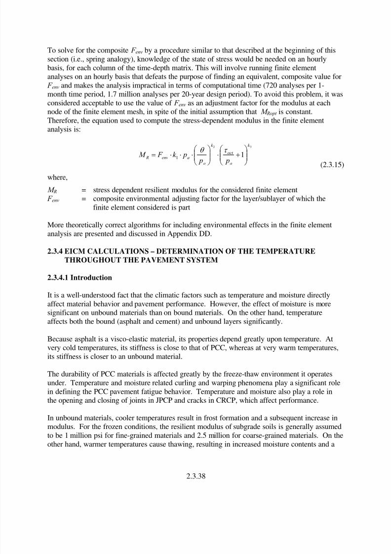
8/6/2019 Chapter3 Environment Effects No Restriction
http://slidepdf.com/reader/full/chapter3-environment-effects-no-restriction 40/52
To solve for the composite F env by a procedure similar to that described at the beginning of this
section (i.e., spring analogy), knowledge of the state of stress would be needed on an hourly
basis, for each column of the time-depth matrix. This will involve running finite elementanalyses on an hourly basis that defeats the purpose of finding an equivalent, composite value for
F env and makes the analysis impractical in terms of computational time (720 analyses per 1-
month time period, 1.7 million analyses per 20-year design period). To avoid this problem, it wasconsidered acceptable to use the value of F env as an adjustment factor for the modulus at eachnode of the finite element mesh, in spite of the initial assumption that M Ropt is constant.
Therefore, the equation used to compute the stress-dependent modulus in the finite element
analysis is:
32
11
k
a
oct
k
a
aenv R p p
pk F M ⎟⎟ ⎠
⎞⎜⎜⎝
⎛ +⋅⎟⎟
⎠
⎞⎜⎜⎝
⎛ ⋅⋅⋅=
τ θ
(2.3.15)
where,
M R
= stress dependent resilient modulus for the considered finite element
F env = composite environmental adjusting factor for the layer/sublayer of which the
finite element considered is part
More theoretically correct algorithms for including environmental effects in the finite element
analysis are presented and discussed in Appendix DD.
2.3.4 EICM CALCULATIONS – DETERMINATION OF THE TEMPERATURE
THROUGHOUT THE PAVEMENT SYSTEM
2.3.4.1 Introduction
It is a well-understood fact that the climatic factors such as temperature and moisture directly
affect material behavior and pavement performance. However, the effect of moisture is moresignificant on unbound materials than on bound materials. On the other hand, temperature
affects both the bound (asphalt and cement) and unbound layers significantly.
Because asphalt is a visco-elastic material, its properties depend greatly upon temperature. Atvery cold temperatures, its stiffness is close to that of PCC, whereas at very warm temperatures,
its stiffness is closer to an unbound material.
The durability of PCC materials is affected greatly by the freeze-thaw environment it operates
under. Temperature and moisture related curling and warping phenomena play a significant role
in defining the PCC pavement fatigue behavior. Temperature and moisture also play a role inthe opening and closing of joints in JPCP and cracks in CRCP, which affect performance.
In unbound materials, cooler temperatures result in frost formation and a subsequent increase inmodulus. For the frozen conditions, the resilient modulus of subgrade soils is generally assumed
to be 1 million psi for fine-grained materials and 2.5 million for coarse-grained materials. On the
other hand, warmer temperatures cause thawing, resulting in increased moisture contents and a
2.3.38

8/6/2019 Chapter3 Environment Effects No Restriction
http://slidepdf.com/reader/full/chapter3-environment-effects-no-restriction 41/52
subsequent decrease in modulus values. During the thawing process, the resilient modulus of
unbound materials may go well below the optimum value (0.5 to 0.85 times M Ropt ).
The CMS and CRREL models in the EICM are primarily responsible for most the temperaturecalculations. A brief overview of these models is presented in this subsection. The ensuing
subsections discuss the temperature calculations in more details. Through this discussion, therelevance of climatic models to the overall pavement design process is brought to fore.Furthermore, the discussion also illustrates how the various climate and materials inputs
discussed in this chapter and elsewhere in this Design Guide are used in the computation of
temperature, moisture, and frost regimes throughout the pavement system.
CMS Model
The CMS model was originally developed at the University of Illinois (1). It is a one-
dimensional, forward finite difference heat transfer model to determine frost penetration and
temperature distribution in the pavement system. The model considers radiation, convection,
conduction, and the effect of latent heat. It does not consider transpiration, condensation,evaporation, or sublimation. These latter effects are neglected because of the uncertainty in their
calculations and because their omission does not create significant errors in the heat balance at
the surface of the pavement. Heat fluxes caused by precipitation and moisture infiltration arealso neglected.
The inputs to the model include:
• Heat capacity of the pavement materials.
• Thermal conductivity of the pavement materials.
• Pavement surface absorptivity and emissivity.
• Air temperature.• Wind speed.
• Incoming solar radiation.
Most of these parameters, with the exception of solar radiation, have been presented and
discussed earlier in this chapter. Solar radiation will be discussed in a later section.
It is worthwhile to note that for pavement layers (AC or PCC), the EICM assumes that the userinput heat capacity and thermal conductivity do not vary over time. However, for unbound
layers (base courses and soils), as the moisture and frost contents change with time, so do the
heat capacity and thermal conductivity. The user input dry heat capacity and dry thermal
conductivity, along with the water and ice content predicted by the EICM, are used to calculatethe wet heat capacity and wet thermal conductivity internally. In this manner the
heat/temperature calculations of the EICM are coupled with the EICM’s moisture predictions.The amount of water held in the soil matrix, whether this held water is in the form of liquid or
ice, directly affects the thermal properties of that material.
The one-dimensional finite difference calculation performed by the CMS model has twoboundaries, the upper boundary that is the pavement surface, and the lower boundary that is the
2.3.39

8/6/2019 Chapter3 Environment Effects No Restriction
http://slidepdf.com/reader/full/chapter3-environment-effects-no-restriction 42/52
constant deep ground temperature node. At the upper boundary, parameters such as air
temperature, wind speed, amount of solar radiation, and pavement absorptivity and emissivity,
determine the quantity of heat flowing into or out of the pavement. The lower boundary is a
constant temperature node, capable of supplying an infinite amount of heat in order to keep thetemperature at that node constant. By modeling the heat flow through the pavement,
temperatures at various depths are easily calculated.
Once the thermal properties that define the heat flow through the pavement and unbound layers
have been established and the boundary conditions have been identified, it is necessary to
determine the amount of heat inflow/outflow at the pavement surface.
The two processes by which heat is added or subtracted from the pavement surface are
convection and radiation, which are discussed below.
Convection Process
Convection is the process of transferring heat energy due to differences in the air temperatureand the pavement surface temperature. If the pavement surface is warmer than air, heat is lost
from the upper boundary. If the pavement surface is colder than the air, heat is added to the
upper boundary. The amount of convection that occurs is directly related to this temperaturedifference and the measured wind speed. Higher wind speeds directly correlate with higher
convection rates.
Radiation Process
The second method of heat flow at the surface is radiation. The primary source of radiation heatflow is short wave solar radiation from the sun. The amount of solar radiation impinging upon
the pavement surface is dependent upon the following factors:
• The position of the sun in the sky.
• The amount of cloud cover.
The latitude of the site being modeled, and the time of the day and year determine the position
of the sun in the sky. These calculations are done internally by the EICM, and require no userinput other than latitude. The amount of cloud cover is a user input and can be obtained from
the climatic database (refer to discussion in section 2.3.2.2). These two variables determine the
amount of solar radiation that is impinging on the pavement surface. The amount of solar
radiation actually absorbed by the pavement is determined by the user input surface shortwave
absorptivity (see section 2.3.2.4 for discussion).
The other type of radiation induced heat flow is long wave radiation. Long wave radiation isthermal radiation that is emitted by the pavement according to black body radiation theory.
Depending on the absolute temperature of a material in degrees Kelvin, a specific amount of heat
energy is emitted in the form of long wave radiation. The EICM assumes a constant value foremissivity for pavements, dependent upon the temperature. A portion of this long wave radiation
emitted by both the pavement and the surrounded landscape is re-absorbed by the pavement,
2.3.40

8/6/2019 Chapter3 Environment Effects No Restriction
http://slidepdf.com/reader/full/chapter3-environment-effects-no-restriction 43/52
after reflecting off of clouds. The method used to determine the amount of long wave radiation
re-absorbed is similar to that employed for short wave radiation.
CRREL Model
The second model used in the Design Guide is the CRREL (2) model. It is a one-dimensionalcoupled heat and moisture flow in the subgrade soil at temperatures that are above, below and atthe freezing temperature of water. In addition, the model predicts the depth of frost and thaw
penetration. It also estimates the vertical heave due to frost formation and vertical settlement
when the soil thaws. The CRREL model uses the temperature profiles through the asphalt layersas established by the CMS model to compute changes in the soil temperature profile, and thus
frost penetration and thaw settlement.
2.3.4.2 Boundary Conditions for CMS Model
Heat Flux Boundary Condition
Temperatures throughout the pavement structure are dominated by atmospheric conditions at the
surface. While it is easy to measure the air temperatures, there is not a direct correspondence
between the air temperatures and pavement surface temperatures. To estimate the pavementtemperature, the energy balance at the surface been used in the CMS model is described as (22,23):
0=±±±−+− g hcear i QQQQQQQ (2.3.16)
where,
Qi = Incoming short wave radiation.
Qr = Reflected short wave radiation. Qa = Incoming long wave radiation.
Qe = Outgoing long wave radiation.
Qc = Convective heat transfer.
Qh = Effects of transpiration, condensation, evaporation, and sublimation.
Q g = Energy absorbed by the ground.
The variables in equation 2.3.16 are illustrated in figure 2.3.10 (3). The net all-wave lengthradiation at the surface is Qn.
l sn QQQ −= (2.3.17)
where,Q s = Net short wave radiation
Ql = Net long wave radiation
r i s QQQ −= (2.3.18)
eal QQQ −= (2.3.19)
2.3.41
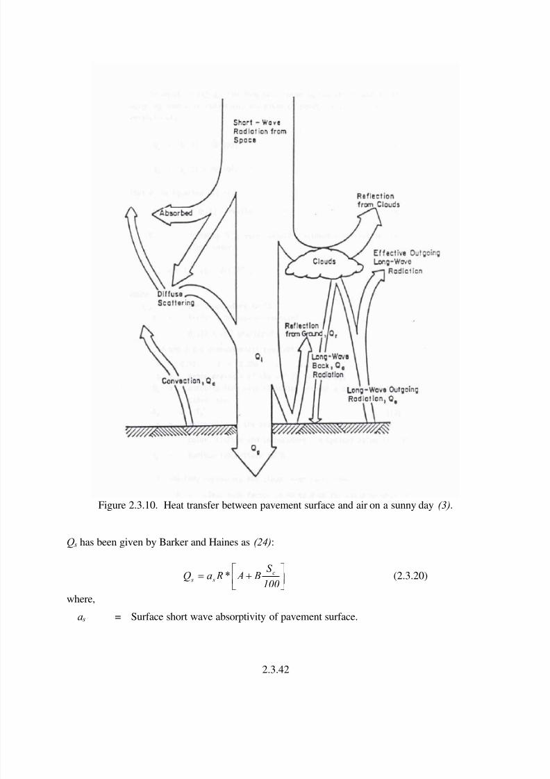
8/6/2019 Chapter3 Environment Effects No Restriction
http://slidepdf.com/reader/full/chapter3-environment-effects-no-restriction 44/52
Figure 2.3.10. Heat transfer between pavement surface and air on a sunny day (3).
Q s has been given by Barker and Haines as (24):
⎥⎦
⎤⎢⎣
⎡+=
100
S B A* RaQ c
s s (2.3.20)
where,
a s = Surface short wave absorptivity of pavement surface.
2.3.42

8/6/2019 Chapter3 Environment Effects No Restriction
http://slidepdf.com/reader/full/chapter3-environment-effects-no-restriction 45/52
R* = Extraterrestrial radiation incident on a horizontal surface at the outer atmosphere.
It depends on the latitude of the site and the solar declination of the sun, which is
the position of the sun north or south of the equator and is a function of the timeof year only.
A, B = Constants that account for diffuse scattering and adsorption by the atmosphere.
The values of A and B for the Midwest have shown to be 0.202 and 0.539,respectively (1).S c = Percentage of sunshine which accounts for the influence of cloud cover.
In equation 2.3.19, Qa, the long wave incoming radiation, and Qe, the outgoing long waveradiation, are given by equations 2.3.21 and 2.3.22.
( )100
NW 1QQ z a −= (2.3.21)
( )100
1 NW QQ xe −= (2.3.22)
Thus Ql in equation 2.3.23 is:
( )( )100
NW 1QQQ x z l −−= (2.3.23)
In equation 2.3.23, Q z is the incoming long wave radiation without a correction for cloud cover
and ( )100
1 NW − represents the cloud cover correction:
pair sb z 10 J GT Q ρ σ −= (2.3.24)
where, N = Cloud base factor (0.9 to 0.80 for cloud heights of 1,000 ft to 6,000 ft (25).W = 100-S c (average cloud cover during day or night).
T air = Air temperature in oR.
σ sb = Stefan-Boltzmann constant, 0.172 x 10⁻⁸ Btu/(hr-ft2-oR).
G = 0.77.
J = 0.28.
ρ = 0.074.
p = Vapor pressure of the air (1 to 10mm Hg).
Q x = Outgoing long wave radiation without a correction for cloud cover
(2.3.25)4 s sb x T Q ε σ =
ε = Emissivity of the pavement which depends on pavement color, texture and
temperature. A typical value is 0.93.
T s = Surface temperature in oR.
2.3.43

8/6/2019 Chapter3 Environment Effects No Restriction
http://slidepdf.com/reader/full/chapter3-environment-effects-no-restriction 46/52
In equation 2.3.16, Qc, the rate of heat transfer by convection, is given by:
F inareT and T T T H Q o
sair sair c )( −= (2.3.26)
where,
H = Convection heat transfer coefficient
This parameter is difficult to determine because of the many variables that influence it. Howeverit can also be expressed as follows (1, 26):
(2.3.27) ] )T T ( 00097 .0U T 00144.0[ 93.122 H 3.0
air s
7 .03.0
m −+=
where,
T s = Surface temperature, in oC.
T air = Air temperature, in oC.
T m = Average of surface and air temperature, in oK.U = Average daily wind speed in m/sec.
The maximum value of the heat transfer coefficient is partly controlled by the stability criteriaestablished for the finite difference approach in computations within the EICM. The suggested
maximum value is 3.0 Btu/(hr-ft2-oF). The effects of transportation, condensation, evaporation
and sublimation (Qh) have been neglected in the formation because they are either too small to besignificant or the effects cancel each other out in the energy balance.
In summary, the above calculations determine the surface temperature and thus control the
temperature throughout the underlying materials. The depth of frost is established by comparing
the computed temperatures with the freezing temperatures of the soil. The depth of frostpenetration has been identified as the position of the 30oF isotherm.
Finally, the finite difference approach is used to determine the nodal temperatures. Details of the
finite difference grid and the formulation of the heat conduction equations are provided in
Reference 1.
Wind Speed
Wind speeds are required in the computations of the convention heat transfer coefficient
described above. Daily speeds required for computations of the convention heat transfer
coefficient are determined by linear interpolation between adjacent months.
Sunshine
Not all the first order weather stations that are used to complete the data for the EICM haverecorded percentage of possible sunshine data. In such situations sunshine data from nearest
station have occasionally been transferred to the location where data are missing. It is felt that
2.3.44

8/6/2019 Chapter3 Environment Effects No Restriction
http://slidepdf.com/reader/full/chapter3-environment-effects-no-restriction 47/52
these modifications should not significantly affect the calculation of heat balance at the surface
of the pavement.
Air Temperature
The description presented earlier shows that heat balance equation requires air temperatures forcalculation of long wave radiation emitted by the air and for the convective heat transfer fromsurface to air. While only maximum and minimum values are recorded by the weather stations,
values for each time step are required for calculations in the EICM. Observations have shown
that temperature variations over a 24-hr period can adequately modeled by a sine wave that hasits minimum value of temperature slightly after sunrise and peaks in the early mid afternoon.
While the times of sunrise may vary significantly with seasons, especially in the more northern
latitudes, a suitable average is computed by the program.
Rainfall
Heat fluxes resulting from precipitation and infiltration into the pavement structure have notbeen considered in formulating the surface heat flux boundary conditions. The role of the
precipitation under these circumstances in not entirely clear, and methods to incorporate it in the
energy balance have not been attempted.
2.3.4.3 Temperature Distribution Profile
After the amount of heat inflow/outflow due to convection and radiation at the pavement surface
is determined, this amount of heat is added/subtracted from the quantity of heat at the upper
boundary. The EICM iterates a single time step, calculating a new temperature profile for thepavement system. This updated temperature profile is used for convection and radiation
calculations at the next time step.
Temperature Data for Flexible Pavement Analysis
For the purpose of the Design Guide a base unit of one month is used for incremental damagecomputations. In situations where the pavement is exposed to freezing and thawing cycles, the
base unit of 1 month is changed to 15 days’ (half month) duration to account for rapid changes in
the pavement material properties during frost/thaw period. It is important to realize that if onlyaverage monthly (or semi-monthly) temperatures are used in the analysis, the effect of extreme
temperatures will not be reflected in the damage computations. The approach adopted in the
Design Guide to circumvent this problem and to include the extreme temperatures during a givenmonth (or during 15 days for freeze/thaw period) is discussed below.
The EICM provides 0.1 hours (6 minutes) temperature over the analysis period. Thistemperature for a given month (or 15-days) can be represented by a normal distribution with a
certain mean value (µ ) and the standard deviation (σ ), N (µ,σ ) as shown in figure 2.3.11.
2.3.45
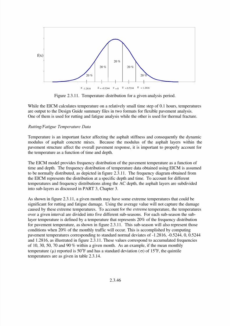
8/6/2019 Chapter3 Environment Effects No Restriction
http://slidepdf.com/reader/full/chapter3-environment-effects-no-restriction 48/52
0
0.05
0.1
0.15
0.2
0.25
0 2 4 6 8 10 12 1 16 18
z = 0
z = 1.2816 z = 0.5244
z = -0.5244z -1.2816
20 %
20 %
20 %
20 %
20 %
f(x)
Figure 2.3.11. Temperature distribution for a given analysis period.
While the EICM calculates temperature on a relatively small time step of 0.1 hours, temperaturesare output to the Design Guide summary files in two formats for flexible pavement analysis.
One of them is used for rutting and fatigue analysis while the other is used for thermal fracture.
Rutting/Fatigue Temperature Data
Temperature is an important factor affecting the asphalt stiffness and consequently the dynamicmodulus of asphalt concrete mixes. Because the modulus of the asphalt layers within the
pavement structure affect the overall pavement response, it is important to properly account for
the temperature as a function of time and depth.
The EICM model provides frequency distribution of the pavement temperature as a function of time and depth. The frequency distribution of temperature data obtained using EICM is assumed
to be normally distributed, as depicted in figure 2.3.11. The frequency diagram obtained from
the EICM represents the distribution at a specific depth and time. To account for differenttemperatures and frequency distributions along the AC depth, the asphalt layers are subdivided
into sub-layers as discussed in PART 3, Chapter 3.
As shown in figure 2.3.11, a given month may have some extreme temperatures that could be
significant for rutting and fatigue damage. Using the average value will not capture the damage
caused by these extreme temperatures. To account for the extreme temperature, the temperaturesover a given interval are divided into five different sub-seasons. For each sub-season the sub-
layer temperature is defined by a temperature that represents 20% of the frequency distribution
for pavement temperature, as shown in figure 2.3.11. This sub-season will also represent those
conditions when 20% of the monthly traffic will occur. This is accomplished by computingpavement temperatures corresponding to standard normal deviates of -1.2816, -0.5244, 0, 0.5244
and 1.2816, as illustrated in figure 2.3.11. These values correspond to accumulated frequencies
of 10, 30, 50, 70 and 90 % within a given month. As an example, if the mean monthly
temperature (µ) reported is 50oF and has a standard deviation (σ) of 15oF, the quintile
temperatures are as given in table 2.3.14.
2.3.46
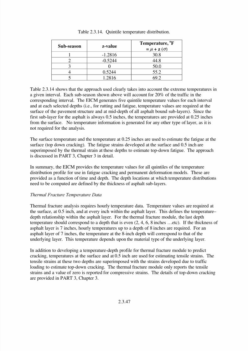
8/6/2019 Chapter3 Environment Effects No Restriction
http://slidepdf.com/reader/full/chapter3-environment-effects-no-restriction 49/52
Table 2.3.14. Quintile temperature distribution.
Sub-season z-valueTemperature,
oF
= µ + z (σ)
1 -1.2816 30.8
2 -0.5244 44.83 0 50.0
4 0.5244 55.2
5 1.2816 69.2
Table 2.3.14 shows that the approach used clearly takes into account the extreme temperatures ina given interval. Each sub-season shown above will account for 20% of the traffic in the
corresponding interval. The EICM generates five quintile temperature values for each interval
and at each selected depths (i.e., for rutting and fatigue, temperature values are required at thesurface of the pavement structure and at mid-depth of all asphalt bound sub-layers). Since the
first sub-layer for the asphalt is always 0.5 inches, the temperatures are provided at 0.25 inches
from the surface. No temperature information is generated for any other type of layer, as it isnot required for the analysis.
The surface temperature and the temperature at 0.25 inches are used to estimate the fatigue at the
surface (top down cracking). The fatigue strains developed at the surface and 0.5 inch aresuperimposed by the thermal strain at these depths to estimate top-down fatigue. The approach
is discussed in PART 3, Chapter 3 in detail.
In summary, the EICM provides the temperature values for all quintiles of the temperature
distribution profile for use in fatigue cracking and permanent deformation models. These are
provided as a function of time and depth. The depth locations at which temperature distributions
need to be computed are defined by the thickness of asphalt sub-layers.
Thermal Fracture Temperature Data
Thermal fracture analysis requires hourly temperature data. Temperature values are required at
the surface, at 0.5 inch, and at every inch within the asphalt layer. This defines the temperature–
depth relationship within the asphalt layer. For the thermal fracture module, the last depthtemperature should correspond to a depth that is even (2, 4, 6, 8 inches …etc). If the thickness of
asphalt layer is 7 inches, hourly temperatures up to a depth of 8 inches are required. For an
asphalt layer of 7 inches, the temperature at the 8-inch depth will correspond to that of theunderlying layer. This temperature depends upon the material type of the underlying layer.
In addition to developing a temperature-depth profile for thermal fracture module to predictcracking, temperatures at the surface and at 0.5 inch are used for estimating tensile strains. The
tensile strains at these two depths are superimposed with the strains developed due to traffic
loading to estimate top-down cracking. The thermal fracture module only reports the tensile
strains and a value of zero is reported for compressive strains. The details of top-down crackingare provided in PART 3, Chapter 3.
2.3.47

8/6/2019 Chapter3 Environment Effects No Restriction
http://slidepdf.com/reader/full/chapter3-environment-effects-no-restriction 50/52
In summary, the EICM will generate a temperature file that defines the temperature–depth
relationship for use in flexible pavement thermal cracking prediction. The file includes
temperature values on an hourly basis for the entire analysis period. The temperatures are usedby the thermal fracture model to predict cracking along with the tensile strains at the surface and
0.5-inch depth for top-down cracking.
Temperature Data for Rigid Pavement Analysis
For rigid pavement design, the main temperature data of interest is the temperature profile
through the PCC layer. EICM is configured to produce hourly temperature profiles for aminimum of one full year. For most sites, EICM climatic database provides 5 years of hourly
data. The data are used in the prediction of faulting and fatigue cracking in JPCP and punchouts
in CRCP.
In the JPCP design module of the Design Guide software, the output from EICM is further
processed to obtain monthly distributions of hourly temperature gradients through PCC. In this
process the nonlinear temperature distribution is first converted to equivalent linear temperaturegradient based on stress equivalence. The equivalent linear temperature gradient is the linear
temperature gradient that would produce the same curling stress as that produced by the actual
nonlinear temperature profile. Thus, the use of equivalent linear temperature gradients does notcause any loss of accuracy in damage calculations; the equivalent linear temperature gradients
are used solely for the purposes of computational efficiency. If climatic data for multiple years
are used, the results are averaged to obtain average monthly distribution of hourly temperaturegradients.
In addition, parameters such as number of freeze-thaw cycles, mean annual precipitation, andmean annual freezing index are also computed from the temperature information for use in the
various JPCP and CRCP structural distress models. Other uses of temperature data include theJPCP joint opening/closing model and the CRCP crack width model.
2.3.48
8/6/2019 Chapter3 Environment Effects No Restriction
http://slidepdf.com/reader/full/chapter3-environment-effects-no-restriction 51/52
REFERENCES
1. Dempsey, B. J., W. A. Herlach, and A. J. Patel (1985). The Climatic-Material-Structural Pavement Analysis Program, FHWA/RD-84/115, Vol.3., Final Report, Federal Highway
Administration, Washington D.C.2. Guymon, G. L., R. L. Berg, and T. C. Johnson (1986). Mathematical Model of Frost Heaveand Thaw Settlement in Pavement, Report: U. S. Army Cold Region Research and
Engineering Laboratory, Hanover, New Hampshire.3. Lytton, R. L., D. E. Pufahl, C. H. Michalak, H. S. Liang, and B. J. Dempsey (1990). An
Integrated Model of the Climatic Effects on Pavement, Texas Transportation Institute, Texas
A&M University, Report No. FHWA-RD-90-033, Federal Highway Administration,
McLean, VA.4. Larson, G., and B. J. Dempsey (1997). Integrated Climatic Model, Version 2.0. Newmark
Civil Engineering Laboratory, University of Illinois at Urbana-Champaign, IL. Report No.
DTFA MN/DOT 72114.5. Witczak, M. W., D. Andrei, and W. N. Houston (2000). Resilient Modulus as Function of
Soil Moisture – Summary of Predictive Models, Development of the 2002 Guide for the
Development of New and Rehabilitated Pavement Structures, NCHRP 1-37 A, Inter TeamTechnical Report (Seasonal 1), Tempe, Arizona.
6. Witczak, M. W., W. N. Houston, and D. Andrei (2000). Resilient Modulus as Function of Soil Moisture – A Study of the Expected Changes in Resilient Modulus of the Unbound Layers with Changes in Moisture for 10 LTPP Sites, Development of the 2002 Guide for the
Development of New and Rehabilitated Pavement Structures, NCHRP 1-37 A, Inter Team
Technical Report (Seasonal 2), Tempe, Arizona.
7. Witczak, M. W., W. N. Houston, and D. Andrei (2000). Selection of Resilient Moduli for Frozen/Thawed Unbound Materials, Development of the 2002 Guide for the Development of
New and Rehabilitated Pavement Structures, NCHRP 1-37 A, Inter Team Technical Report(Seasonal 3), Tempe, Arizona.
8. Witczak, M. W., W. N. Houston, C. E. Zapata, C. Richter, G. Larson, and K. Walsh. (June
2000). Improvement of the Integrated Climatic Model for Moisture Content Predictions,Development of the 2002 Guide for the Development of New and Rehabilitated Pavement
Structures, NCHRP 1-37 A, Inter Team Technical Report (Seasonal 4), Tempe, Arizona.
9. Fredlund, D. G., and A. Xing (1994). “Equations for the Soil-Water Characteristic Curve”,Canadian Geotechnical Journal, Vol. 31, No. 4, pp. 521 - 532.
10. Fredlund, D. G., A. Xing, and S. Huang (1994). “Predicting the Permeability Function for Unsaturated Soils Using the Soil-Water Characteristic Curve”, Canadian GeotechnicalJournal, Vol 3., No. 4, pp. 533 - 546.
11. Fredlund, D. G., A. Xing, M. Fredlund, and S. L. Barbour (1995). “The Relationship of the Unsaturated Shear Strength to the Soil-Water Characteristic Curve”, Canadian GeotechnicalJournal, Vol. 32, pp. 440-448.
12. Leong, E. C., and H. Rahardjo (1996). A Review on Soil-Water Characteristic Curve Equations, Geotechnical Research Report, NTU/GT/96-5, Nanyang Technological
University, NTU-PWD Geotechnical Research Center, Singapore.13. Zapata, C. E. (1999). Uncertainty in Soil-Water Characteristic Curve and Impacts on
Unsaturated Shear Strength Predictions, Ph. D. Dissertation, Arizona State University,
Tempe, AZ.
2.3.49
8/6/2019 Chapter3 Environment Effects No Restriction
http://slidepdf.com/reader/full/chapter3-environment-effects-no-restriction 52/52
14. Schoeneberger, P.J., D. A. Wysocki, E. C. Benham, and W. D. Broderson (1998). Field Book for Describing and Sampling Soils (Version 1.1, refined, revised, and compiled).
National Soil Survey Center, Natural Resources Conservation Service, U.S. Department of Agriculture, Lincoln, NE.
15. Williams, P. J. (1982). The Surface of the Earth, An Introduction to Geotechnical Science.
Longman, Inc., New York.16. Lekarp, F., U. Isacsson, and A. Dawson (2000). “State of the Art I: Resilient Response of Unbound Aggregates , ASCE Journal of Transportation Engineering, Vol. 126, No. 1, pp. 76-
83.
17. Li, D., and E. T. Selig (1994). “Resilient Modulus for Fine Grained Subgrade Soils” , ASCEJournal of Geotechnical Engineering, Vol. 120, No. 6, pp. 939-957.
18. Drumm, E. C., J. S. Reeves, M. R. Madgett, and W. D. Trolinger (July 1997). “Subgrade Resilient Modulus Correction for Saturation Effects” ASCE Journal of Geotechnical andGeoenvironmental Engineering, Vol. 123, No. 7, pp. 663-670.
19. Rada, G., and M. W. Witczak (1981). Comprehensive Evaluation of Laboratory Resilient Moduli Results for Granular Material , Transportation Research Record 810, TRB, National
Research Council, Washington, D.C., pp. 23-33.20. Santha, B.L. 1994. “Resilient Modulus of Subgrade Soils: Comparison of Two Constitutive Equations”, Transportation Research Record 1462, TRB, National Research Council,
Washington, D.C., pp. 79-90.21. Fredlund, D.G., and H. Rahardjo (1993). Soil Mechanics for Unsaturated Soils, John Wiley
& Sons, Inc.
22. Scott, R. F. (1964). Heat Exchange at the Ground Surface, U. S. Army Material Command,Cold Regions Research and Engineering Laboratory, Hanover, N. H.
23. Berg, R. L. (1968). Energy Balance on Paved Surface, U. S. Army Terrestrial Sciences
Center, Hanover, NH.24. Baker, D. G., and D. A. Haines (1969). Solar Radiation and Sunshine Duration Relationship
in the North-Central Region and Alaska, Experiment Station, University of Minnesota,Minneapolis, MN, Technical Bulletin 262.
25. Geiger, R. (1959). The Climate Near Ground, Harvard University Press, Cambridge, MA.
26. Vehrencamp, J. E. (1953). Experimental Investigation of Heat Transfer at Air-Earth Interface, Transportation, American Geophysical Union, Washington, D.C.,Vol. 34, No. 1.