Chapter6-Galoppo-Dynamic Deformation Texturesdeveloper.amd.com/.../02/Chapter6-Galoppo-Dynamic_Deformation_… · We have implemented this parallel implicit contact resolution method

Advanced Real-Time Rendering in 3D Graphics and Games Course – SIGGRAPH 2007

59

Chapter 6

Dynamic Deformation Textures GPU-Accelerated Simulation of Deformable

Models in Contact

Nico Galoppo8 UNC Chapel Hill

Miguel A. Otaduy9

ETH Zurich Paul Mecklenburg10

UNC Chapel Hill

Markus Gross11

ETH Zurich

Ming C. Lin12 UNC Chapel Hill

Figure 1. Soft Object Interaction in a Dynamic Scene. Deformable objects roll and collide in the playground. In these simulations, over 15,000 contacts were processed per second. 8 email: [email protected] 9 email: [email protected] 10 email: [email protected] 11 email: [email protected] 12 email: [email protected]

Chapter 6: Dynamic Deformation Textures

60

6.1 Introduction We present an efficient algorithm for simulating contacts between deformable bodies with high-resolution surface geometry using dynamic deformation textures (D2Ts), which reformulate the 3D elastoplastic deformation and collision handling on a 2D parametric atlas to reduce the extremely high number of degrees of freedom arising from large contact regions and high-resolution geometry. Such computationally challenging dynamic contact scenarios arise when objects with rich surface geometry are rubbed against each other while they bounce, roll or slide through the scene, as shown in Figure 1. We simulate real-world deformable solids that can be modeled as a rigid core covered by a layer of deformable material [TW88], assuming that the deformation field of the surface can be expressed as a function in the parametric domain of the rigid core. Examples include animated characters, furniture, toys, tires, etc. Our mathematical formulation of dynamic simulation and contact processing, along with the use of dynamic deformation textures, is especially well suited for realization on commodity SIMD or parallel architectures, such as graphics processing units (GPU), Cell processors, and physics processing units (PPU). More in particular, the following key concepts contribute to the mapping of our algorithm to the GPU architecture, resulting in the effectiveness and efficiency of our algorithm:

x We reformulate the 3-dimensional elastoplastic deformations and collision processing on 2-dimensional dynamic deformation textures. This mapping is illustrated in Figures 3 and 8, with the 2D computational domains indicated by T and D. There is a natural mapping between the computational domains and graphics hardware textures.

x Using a two-stage collision detection algorithm for parameterized layered

deformable models, our proximity queries are scalable and output-sensitive, i.e. the performance of the queries does not directly depend on the complexity of the surface meshes. We perform high resolution collision detection with an image based collision detection algorithm, implemented on the GPU.

x By decoupling the parallel update of surface displacements and parallel

constraint-based collision response from the update of the core DoFs, we provide fast and responsive simulations under large time steps on heterogeneous materials. We have implemented this parallel implicit contact resolution method on the GPU, thereby exploiting the inherent parallelism of the GPU architecture.

A common thread throughout the design of our algorithm is the desire to minimize data transfer between GPU and CPU while maximizing the parallel computation power of the GPU. In our algorithm, surface simulation, collision detection and rendering are all performed by the GPU exploiting our common D2T model representation. The surface deformation is simulated very efficiently on the GPU in fragment programs and updated in texture memory. A dynamically changing position texture is thus available for collision detection and rendering.


61

6.2 Algorithm Overview and Parallel Implementation

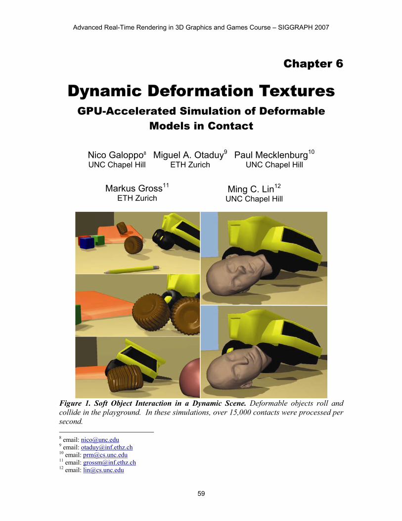
Figure 2. Algorithm Overview.

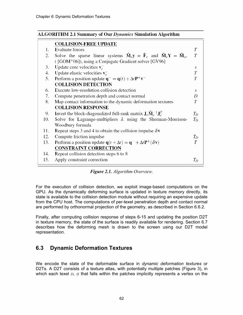
The implicit formulation of the dynamic motion equations and collision response yields linear systems of equations with dense coupling between the core and elastic velocities. However, we can formulate the velocity update and collision response in a highly parallelizable manner [GOM+06]. In Figure 2 we illustrate how our algorithm for simulating and rendering deformable objects in contact using dynamic deformation textures maps to the GPU. Algorithm 2.1 shows a more detailed breakdown of the steps of the dynamics computations. We refer the interested reader to [GOM+06] for details of the equations. Let s in Algorithm 2.1 denote the operations that are performed on small-sized systems (i.e., computations of core variables, and low resolution collision detection). The remaining operations are all executed in a parallel manner on a large number of simulation nodes. Specifically, T refers to operations to be executed on all simulation nodes in the dynamic deformation texture T, D refers to operations to be executed on texels of the contact plane D, and TD refers to operations to be executed on the colliding nodes. As highlighted in Algorithm 2.1, all operations to be executed on simulation nodes (indicated by T, TD and D) can be implemented with parallelizable computation stencils on the GPU, as indicated in Figure 2 by purple diamond boxes. Moreover, due to the regular meshing of the deformable layer produced by dynamic deformation textures, the computation stencils are uniform across all nodes; hence they are amenable to implementation on a streaming processor such as the GPU. In Section 6.5 we will illustrate this concept for representing and computing sparse matrix multiplications in step 2 of Algorithm 2.1.


62

Figure 2.1. Algorithm Overview.

For the execution of collision detection, we exploit image-based computations on the GPU. As the dynamically deforming surface is updated in texture memory directly, its state is available to the collision detection module without requiring an expensive update from the CPU host. The computations of per-texel penetration depth and contact normal are performed by orthonormal projection of the geometry, as described in Section 6.6.2. Finally, after computing collision response of steps 6-15 and updating the position D2T in texture memory, the state of the surface is readily available for rendering. Section 6.7 describes how the deforming mesh is drawn to the screen using our D2T model representation. 6.3 Dynamic Deformation Textures We encode the state of the deformable surface in dynamic deformation textures or D2Ts. A D2T consists of a texture atlas, with potentially multiple patches (Figure 3), in which each texel (s, t) that falls within the patches implicitly represents a vertex on the


63

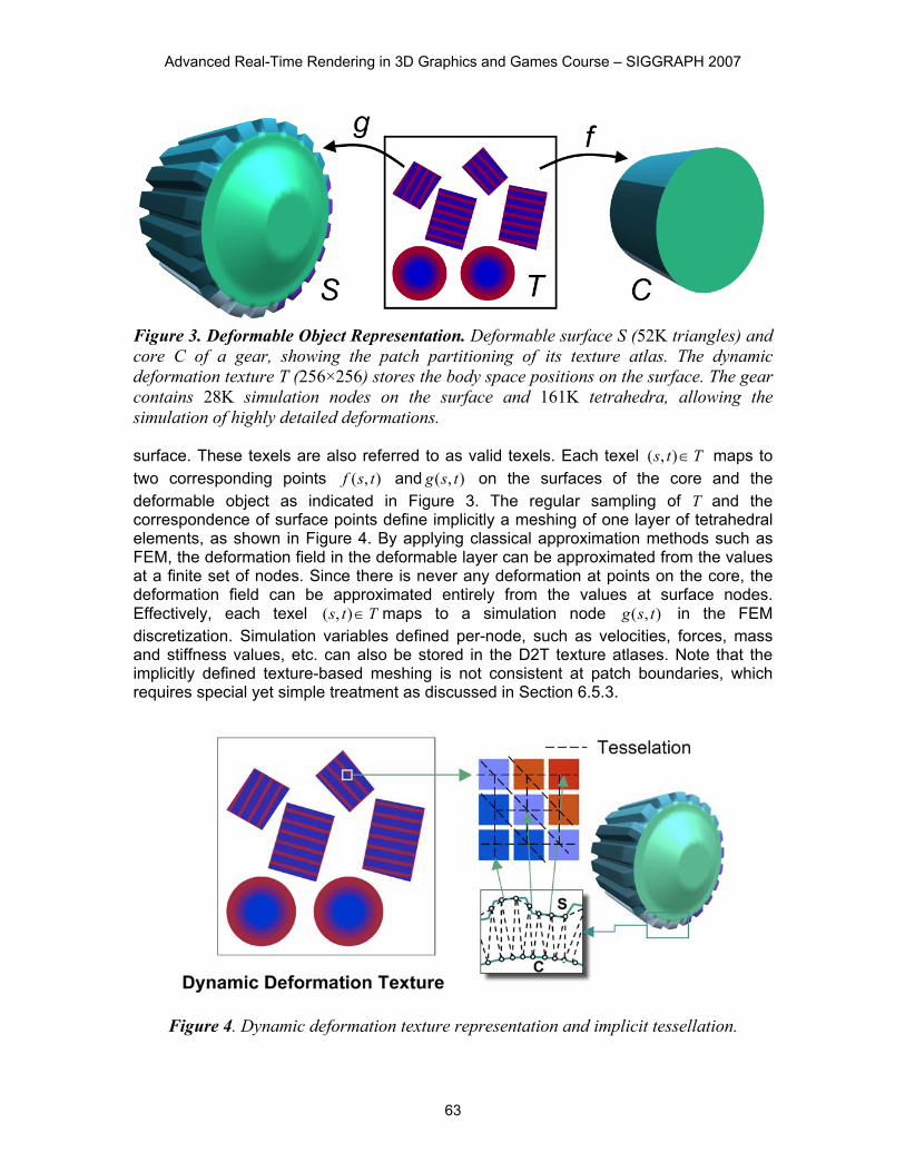
Figure 3. Deformable Object Representation. Deformable surface S (52K triangles) and core C of a gear, showing the patch partitioning of its texture atlas. The dynamic deformation texture T (256×256) stores the body space positions on the surface. The gear contains 28K simulation nodes on the surface and 161K tetrahedra, allowing the simulation of highly detailed deformations. surface. These texels are also referred to as valid texels. Each texel Tts �),( maps to two corresponding points ),( tsf and ),( tsg on the surfaces of the core and the deformable object as indicated in Figure 3. The regular sampling of T and the correspondence of surface points define implicitly a meshing of one layer of tetrahedral elements, as shown in Figure 4. By applying classical approximation methods such as FEM, the deformation field in the deformable layer can be approximated from the values at a finite set of nodes. Since there is never any deformation at points on the core, the deformation field can be approximated entirely from the values at surface nodes. Effectively, each texel Tts �),( maps to a simulation node ),( tsg in the FEM discretization. Simulation variables defined per-node, such as velocities, forces, mass and stiffness values, etc. can also be stored in the D2T texture atlases. Note that the implicitly defined texture-based meshing is not consistent at patch boundaries, which requires special yet simple treatment as discussed in Section 6.5.3.

Figure 4. Dynamic deformation texture representation and implicit tessellation.


64

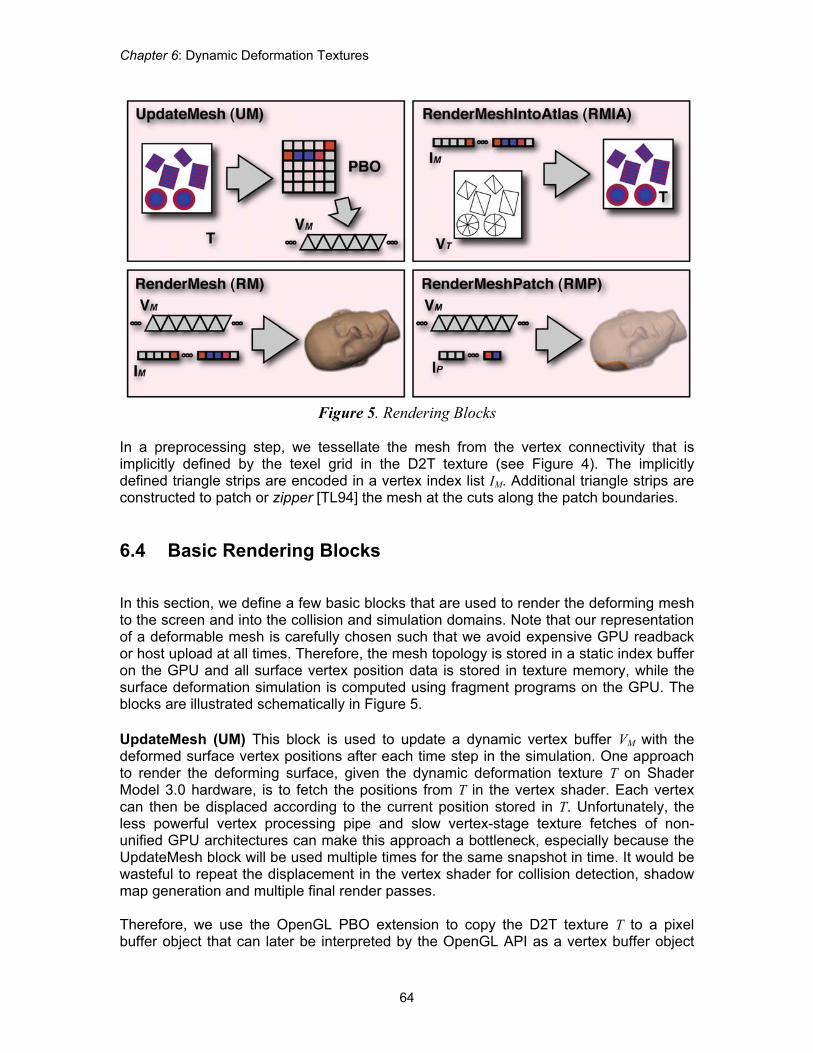
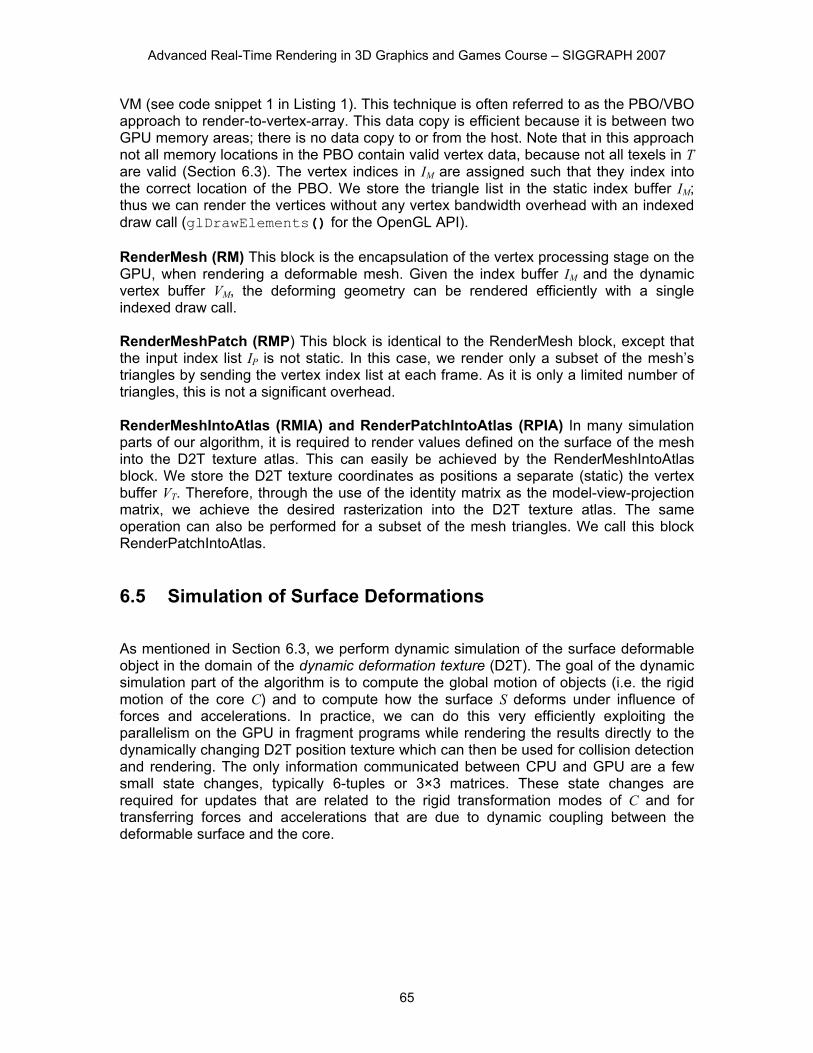
Figure 5. Rendering Blocks

In a preprocessing step, we tessellate the mesh from the vertex connectivity that is implicitly defined by the texel grid in the D2T texture (see Figure 4). The implicitly defined triangle strips are encoded in a vertex index list IM. Additional triangle strips are constructed to patch or zipper [TL94] the mesh at the cuts along the patch boundaries. 6.4 Basic Rendering Blocks In this section, we define a few basic blocks that are used to render the deforming mesh to the screen and into the collision and simulation domains. Note that our representation of a deformable mesh is carefully chosen such that we avoid expensive GPU readback or host upload at all times. Therefore, the mesh topology is stored in a static index buffer on the GPU and all surface vertex position data is stored in texture memory, while the surface deformation simulation is computed using fragment programs on the GPU. The blocks are illustrated schematically in Figure 5. UpdateMesh (UM) This block is used to update a dynamic vertex buffer VM with the deformed surface vertex positions after each time step in the simulation. One approach to render the deforming surface, given the dynamic deformation texture T on Shader Model 3.0 hardware, is to fetch the positions from T in the vertex shader. Each vertex can then be displaced according to the current position stored in T. Unfortunately, the less powerful vertex processing pipe and slow vertex-stage texture fetches of non-unified GPU architectures can make this approach a bottleneck, especially because the UpdateMesh block will be used multiple times for the same snapshot in time. It would be wasteful to repeat the displacement in the vertex shader for collision detection, shadow map generation and multiple final render passes. Therefore, we use the OpenGL PBO extension to copy the D2T texture T to a pixel buffer object that can later be interpreted by the OpenGL API as a vertex buffer object


65

VM (see code snippet 1 in Listing 1). This technique is often referred to as the PBO/VBO approach to render-to-vertex-array. This data copy is efficient because it is between two GPU memory areas; there is no data copy to or from the host. Note that in this approach not all memory locations in the PBO contain valid vertex data, because not all texels in T are valid (Section 6.3). The vertex indices in IM are assigned such that they index into the correct location of the PBO. We store the triangle list in the static index buffer IM; thus we can render the vertices without any vertex bandwidth overhead with an indexed draw call (glDrawElements() for the OpenGL API). RenderMesh (RM) This block is the encapsulation of the vertex processing stage on the GPU, when rendering a deformable mesh. Given the index buffer IM and the dynamic vertex buffer VM, the deforming geometry can be rendered efficiently with a single indexed draw call. RenderMeshPatch (RMP) This block is identical to the RenderMesh block, except that the input index list IP is not static. In this case, we render only a subset of the mesh’s triangles by sending the vertex index list at each frame. As it is only a limited number of triangles, this is not a significant overhead. RenderMeshIntoAtlas (RMIA) and RenderPatchIntoAtlas (RPIA) In many simulation parts of our algorithm, it is required to render values defined on the surface of the mesh into the D2T texture atlas. This can easily be achieved by the RenderMeshIntoAtlas block. We store the D2T texture coordinates as positions a separate (static) the vertex buffer VT. Therefore, through the use of the identity matrix as the model-view-projection matrix, we achieve the desired rasterization into the D2T texture atlas. The same operation can also be performed for a subset of the mesh triangles. We call this block RenderPatchIntoAtlas. 6.5 Simulation of Surface Deformations As mentioned in Section 6.3, we perform dynamic simulation of the surface deformable object in the domain of the dynamic deformation texture (D2T). The goal of the dynamic simulation part of the algorithm is to compute the global motion of objects (i.e. the rigid motion of the core C) and to compute how the surface S deforms under influence of forces and accelerations. In practice, we can do this very efficiently exploiting the parallelism on the GPU in fragment programs while rendering the results directly to the dynamically changing D2T position texture which can then be used for collision detection and rendering. The only information communicated between CPU and GPU are a few small state changes, typically 6-tuples or 3×3 matrices. These state changes are required for updates that are related to the rigid transformation modes of C and for transferring forces and accelerations that are due to dynamic coupling between the deformable surface and the core.


66

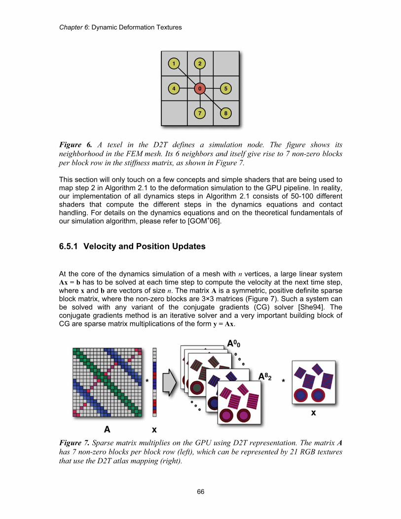
Figure 6. A texel in the D2T defines a simulation node. The figure shows its neighborhood in the FEM mesh. Its 6 neighbors and itself give rise to 7 non-zero blocks per block row in the stiffness matrix, as shown in Figure 7. This section will only touch on a few concepts and simple shaders that are being used to map step 2 in Algorithm 2.1 to the deformation simulation to the GPU pipeline. In reality, our implementation of all dynamics steps in Algorithm 2.1 consists of 50-100 different shaders that compute the different steps in the dynamics equations and contact handling. For details on the dynamics equations and on the theoretical fundamentals of our simulation algorithm, please refer to [GOM+06].

6.5.1 Velocity and Position Updates At the core of the dynamics simulation of a mesh with n vertices, a large linear system Ax = b has to be solved at each time step to compute the velocity at the next time step, where x and b are vectors of size n. The matrix A is a symmetric, positive definite sparse block matrix, where the non-zero blocks are 3×3 matrices (Figure 7). Such a system can be solved with any variant of the conjugate gradients (CG) solver [She94]. The conjugate gradients method is an iterative solver and a very important building block of CG are sparse matrix multiplications of the form y = Ax.

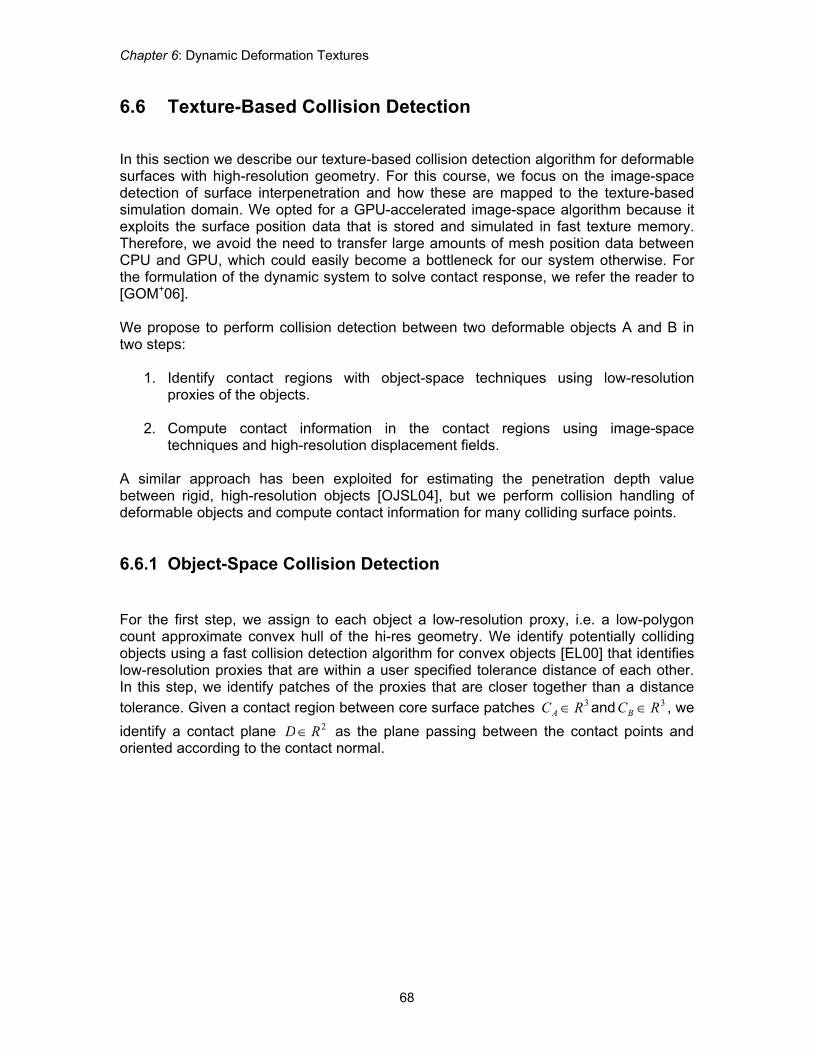
Figure 7. Sparse matrix multiplies on the GPU using D2T representation. The matrix A has 7 non-zero blocks per block row (left), which can be represented by 21 RGB textures that use the D2T atlas mapping (right).


67

In the remainder of this section, we will explain how A is stored and how these sparse matrix multiplies are performed in a fragment program.

6.5.2 Sparse Matrix Representation and Multiplication The vectors x and y nR3� both define vector values (3-tuples) at each vertex. We already know from Section 6.3 that we can store those values at valid texels in the D2T texture atlas. We can also map A to the D2T atlas as follows. Each block row of A defines seven 3×3 blocks, one for each neighbor of a given vertex (or texel in the D2T) as shown in Figure 6. Hence, we can store A in 21 RGB textures where each texture stores a 3×1 row of a 3×3 block (Figure 7). Due to the limited number of texture samplers that can be bound to a fragment program within a pass, the actual sparse matrix multiplication has to be performed in two passes. Mathematically, this corresponds to the following transformation: Ax = > Al Ar @x = Alx + Arx. In the second pass, the result of Alx is passed in from the first pass. Code Snippet 2 in Listing 2 shows the setup and invocation of the passes, while Fragment Programs 1 and 2 (Listing 3 and 4) show the implementation in the fragment processor. Note that if x is an n×3 matrix instead of a vector of size n, the result is an n×3 matrix. This can still be achieved in 2 passes by rendering to multiple render targets simultaneously, storing 3 columns instead of 1. This approach of matrix multiplies is very efficient on parallel streaming processors such as current GPUs, because there is no branching or pointer chasing involved. Moreover, our mapping of the sparse matrix to the D2T atlas exploits the GPU texture caching architecture in two ways. First, due to tile based rendering, neighboring values fetched from x and A in one fragment are conveniently pulled into cache for neighboring fragments in the same tile. Second, fetching a value pulls in other neighboring values from x and A that are required in the same fragment program for free.

6.5.3 Patch Boundary Handling In the previous section, we have neglected the fact that, at patch boundaries in the D2T, not all neighboring texels are valid texels. One solution could be to flag boundary texels in some way and use branching that is available in current GPU hardware, but this is not very efficient because the boundaries are not coherent fragment blocks. Better approaches are to rasterize and handle the boundary texels separately with a separate fragment program [Har05] or to guarantee that all neighbors are valid. We have taken the latter approach. We adapt a method by Stam [Sta03] for providing accessible data in an 8-neighborhood to all nodes located on patch boundaries. Before every sparse matrix multiplication step in the algorithm, we fill a 2 -texel-width region on patch boundaries by sampling values on the adjacent patches. In practice, for each deformable model and D2T atlas, we maintain a list of thin quads that have texture coordinates assigned that map to locations of neighboring surface points across boundaries in the D2T texture atlas.


68

6.6 Texture-Based Collision Detection In this section we describe our texture-based collision detection algorithm for deformable surfaces with high-resolution geometry. For this course, we focus on the image-space detection of surface interpenetration and how these are mapped to the texture-based simulation domain. We opted for a GPU-accelerated image-space algorithm because it exploits the surface position data that is stored and simulated in fast texture memory. Therefore, we avoid the need to transfer large amounts of mesh position data between CPU and GPU, which could easily become a bottleneck for our system otherwise. For the formulation of the dynamic system to solve contact response, we refer the reader to [GOM+06]. We propose to perform collision detection between two deformable objects A and B in two steps:

1. Identify contact regions with object-space techniques using low-resolution proxies of the objects.

2. Compute contact information in the contact regions using image-space

techniques and high-resolution displacement fields.

A similar approach has been exploited for estimating the penetration depth value between rigid, high-resolution objects [OJSL04], but we perform collision handling of deformable objects and compute contact information for many colliding surface points.

6.6.1 Object-Space Collision Detection For the first step, we assign to each object a low-resolution proxy, i.e. a low-polygon count approximate convex hull of the hi-res geometry. We identify potentially colliding objects using a fast collision detection algorithm for convex objects [EL00] that identifies low-resolution proxies that are within a user specified tolerance distance of each other. In this step, we identify patches of the proxies that are closer together than a distance tolerance. Given a contact region between core surface patches 3RCA � and 3RCB � , we identify a contact plane 2RD� as the plane passing between the contact points and oriented according to the contact normal.


69

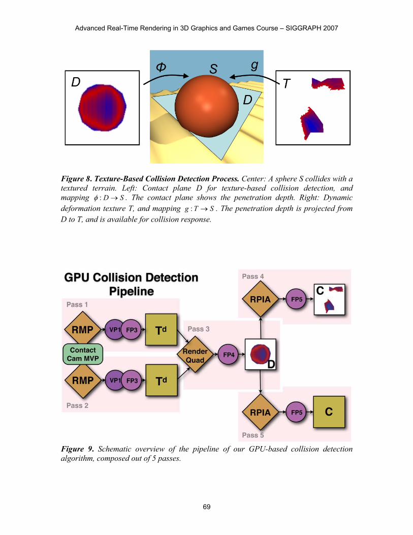
Figure 8. Texture-Based Collision Detection Process. Center: A sphere S collides with a textured terrain. Left: Contact plane D for texture-based collision detection, and mapping SD o:I . The contact plane shows the penetration depth. Right: Dynamic deformation texture T, and mapping STg o: . The penetration depth is projected from D to T, and is available for collision response.

Figure 9. Schematic overview of the pipeline of our GPU-based collision detection algorithm, composed out of 5 passes.


70

6.6.2 Image-Space Collision Detection The second step in our algorithm is accelerated by the GPU. This stage utilizes the RenderMeshPatch block (Section 6.4). We restrict the draw call to the triangles that form the potentially colliding surface patch. Our image-based algorithm consists of three substeps that are implemented by five rendering passes per pair of potentially colliding surface patches (Figure 9). In the first two passes, we perform a projection step for each potentially colliding surface patch. We set up an orthographic projection which we call the contact camera. The contact camera is carefully positioned such that it looks along the normal of the contact plane D and such that the projections CA and CB capture the full extent of the contact area of a pair of potentially colliding surface patches SA and SB (Figure 10). Vertex Program 1 (Listing 5) and Fragment Program 3 (Listing 6) are used to rasterize the distance from the eye directly into textures d

AT and dBT . Note that we enable front-facing

triangles while rasterizing SA into dAT and back-facing triangles while rasterizing SB into

dBT . In the third pass, we capture the areas of interpenetrating surface patches by

constructing texture D from projections dAT and d

BT . For each texel Dvu �),( , we perform high-resolution collision detection by testing the distance between points

AA SvuC �),( and BB SvuC �),( along the normal direction of D. If the points are penetrating, we identify a contact constraint and we compute the contact normal n as the average surface normal. We also approximate the penetration depth as

)),(),(( vuTvuTd ABT � n for applying constraint correction. This approximation is

affected by texture distortion as the surface deforms, but we have not found noticeable errors in our examples. In practice, as shown in the middle of Figure 9, we render a full-screen quad of the size of d

AT and dBT into D, while Fragment Program 4 (Listing 7)

computes the difference in distances. Positive values indicate penetration in the projection as indicated by the red regions on the left in Figure 8. Note that we also write the triangle ID of the current fragment to D. These IDs are used in the next pass to check whether a rasterized texel of the D2T is originating from the triangle whose fragments were rasterized into D and not from a triangle that maps to the same texel in D (see Figure 10). Recall that the deformation of the sphere is stored in the two-dimensional texture atlas T called dynamic deformation texture (D2T). This texture atlas is shown on the right in Figure 8. We compute dynamic contact response in this domain. Therefore, the collision information in texture D has to be transferred to the dynamic deformation texture T via a mapping that is the combination of the inverse of the orthogonal contact projection with the D2T texture atlas mapping. In practice, this step is performed by the two last passes of our algorithm. These passes render each potentially surface geometry again using the RenderMeshIntoAtlas block (Section 6.4) into the D2T domain. We set up the texture matrix to perform the correct mapping while fetching values from texture D. The required texture matrix set up is completely analogous to the typical setup for traditional shadow mapping. Here, the contact camera model-view-projection matrix takes the place of the light’s model-view-projection matrix. Code Snippet 3 in Listing 9 shows the code that is


71

used for this setup. Fragment Program 5 (Listing 8) shows the pixel shader code of the last two passes, one shader per object.

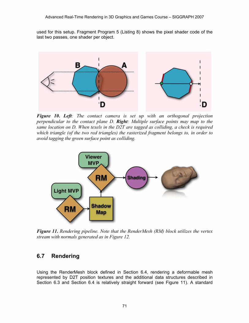
Figure 10. Left: The contact camera is set up with an orthogonal projection perpendicular to the contact plane D. Right: Multiple surface points may map to the same location on D. When texels in the D2T are tagged as colliding, a check is required which triangle (of the two red triangles) the rasterized fragment belongs to, in order to avoid tagging the green surface point as colliding.

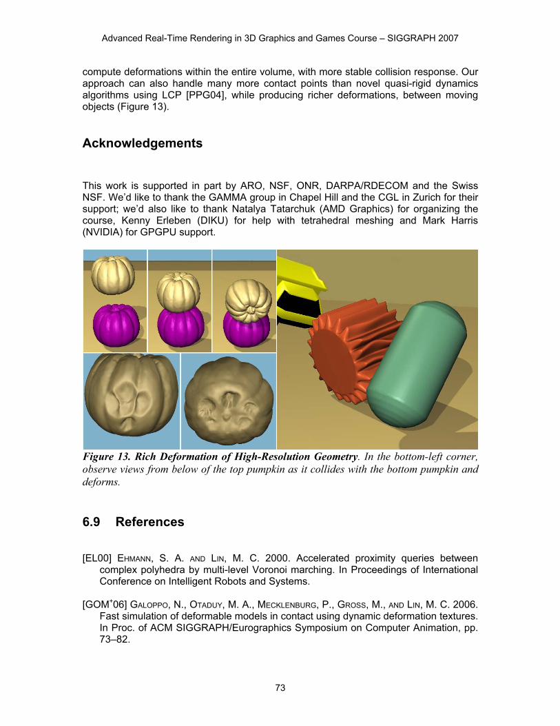
Figure 11. Rendering pipeline. Note that the RenderMesh (RM) block utilizes the vertex stream with normals generated as in Figure 12. 6.7 Rendering Using the RenderMesh block defined in Section 6.4, rendering a deformable mesh represented by D2T position textures and the additional data structures described in Section 6.3 and Section 6.4 is relatively straight forward (see Figure 11). A standard


72

fragment program that computes per-pixel shading is plugged into the pipeline and the RenderMesh block can also be used to generate a standard shadow map. The only missing piece of information are the vertex normals. As the geometry is deforming, normals have to be recomputed at each frame (or each few frames). There are two approaches possible. On Shader Model 4.0 (DirectX10) compatible hardware, the normals can be computed in a geometry shader provided that an appropriate triangle adjacency list is sent to the GPU. Alternatively, on older hardware, one can generate a normal map using the D2T texture atlas. This process is illustrated in Figure 12 along with Fragment Program 6 (Listing 10). Here, as for sparse matrix multiplication in Section 6.5.2, the input D2T texture has to be augmented with replicated position information along the patch boundaries. This ensures that each D2T texel neighborhood is valid and can be sampled to approximate the corresponding vertex normal. The normals vertex buffer can be updated with the normal map using the PBO technique that was also used when updating the position vertex buffer in Section 6.4.

Figure 12. Normal Generation block. A normals PBO is generated and then copied to the normal vertex buffer. 6.8 Results In Figure 1, we show a scene where deformable tires with high-resolution features on their surfaces roll, bounce, and collide with each other. This simulation consists of 324K tetrahedra and 62K surface simulation nodes. Such high resolution enables the simulation of rich deformations, as shown in the accompanying video. All contacts on the surface have global effect on the entire deformable layer, they are processed simultaneously and robustly. Without any precomputation of dynamics or significant storage requirement, we were able to simulate this scene, processing over 15,000 contacts per second, on a 3.4 GHz P4 with NVIDIA GeForce 7800. Our approach is considerably faster than other methods that enable large time steps, such as those that focus on the surface deformation and corotational methods that


73

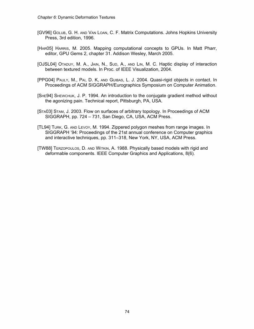
compute deformations within the entire volume, with more stable collision response. Our approach can also handle many more contact points than novel quasi-rigid dynamics algorithms using LCP [PPG04], while producing richer deformations, between moving objects (Figure 13). Acknowledgements This work is supported in part by ARO, NSF, ONR, DARPA/RDECOM and the Swiss NSF. We’d like to thank the GAMMA group in Chapel Hill and the CGL in Zurich for their support; we’d also like to thank Natalya Tatarchuk (AMD Graphics) for organizing the course, Kenny Erleben (DIKU) for help with tetrahedral meshing and Mark Harris (NVIDIA) for GPGPU support.

Figure 13. Rich Deformation of High-Resolution Geometry. In the bottom-left corner, observe views from below of the top pumpkin as it collides with the bottom pumpkin and deforms. 6.9 References [EL00] EHMANN, S. A. AND LIN, M. C. 2000. Accelerated proximity queries between

complex polyhedra by multi-level Voronoi marching. In Proceedings of International Conference on Intelligent Robots and Systems.

[GOM+06] GALOPPO, N., OTADUY, M. A., MECKLENBURG, P., GROSS, M., AND LIN, M. C. 2006.

Fast simulation of deformable models in contact using dynamic deformation textures. In Proc. of ACM SIGGRAPH/Eurographics Symposium on Computer Animation, pp. 73–82.


74

[GV96] GOLUB, G. H. AND VAN LOAN, C. F. Matrix Computations. Johns Hopkins University Press, 3rd edition, 1996.

[HAR05] HARRIS, M. 2005. Mapping computational concepts to GPUs. In Matt Pharr,

editor, GPU Gems 2, chapter 31. Addison Wesley, March 2005. [OJSL04] OTADUY, M. A., JAIN, N., SUD, A., AND LIN, M. C. Haptic display of interaction

between textured models. In Proc. of IEEE Visualization, 2004. [PPG04] PAULY, M., PAI, D. K, AND GUIBAS, L. J. 2004. Quasi-rigid objects in contact. In

Proceedings of ACM SIGGRAPH/Eurographics Symposium on Computer Animation. [SHE94] SHEWCHUK, J. P. 1994. An introduction to the conjugate gradient method without

the agonizing pain. Technical report, Pittsburgh, PA, USA. [STA03] STAM, J. 2003. Flow on surfaces of arbitrary topology. In Proceedings of ACM

SIGGRAPH, pp. 724 – 731, San Diego, CA, USA, ACM Press. [TL94] TURK, G. AND LEVOY, M. 1994. Zippered polygon meshes from range images. In

SIGGRAPH ’94: Proceedings of the 21st annual conference on Computer graphics and interactive techniques, pp. 311–318, New York, NY, USA, ACM Press.

[TW88] TERZOPOULOS, D. AND WITKIN, A. 1988. Physically based models with rigid and

deformable components. IEEE Computer Graphics and Applications, 8(6).


75

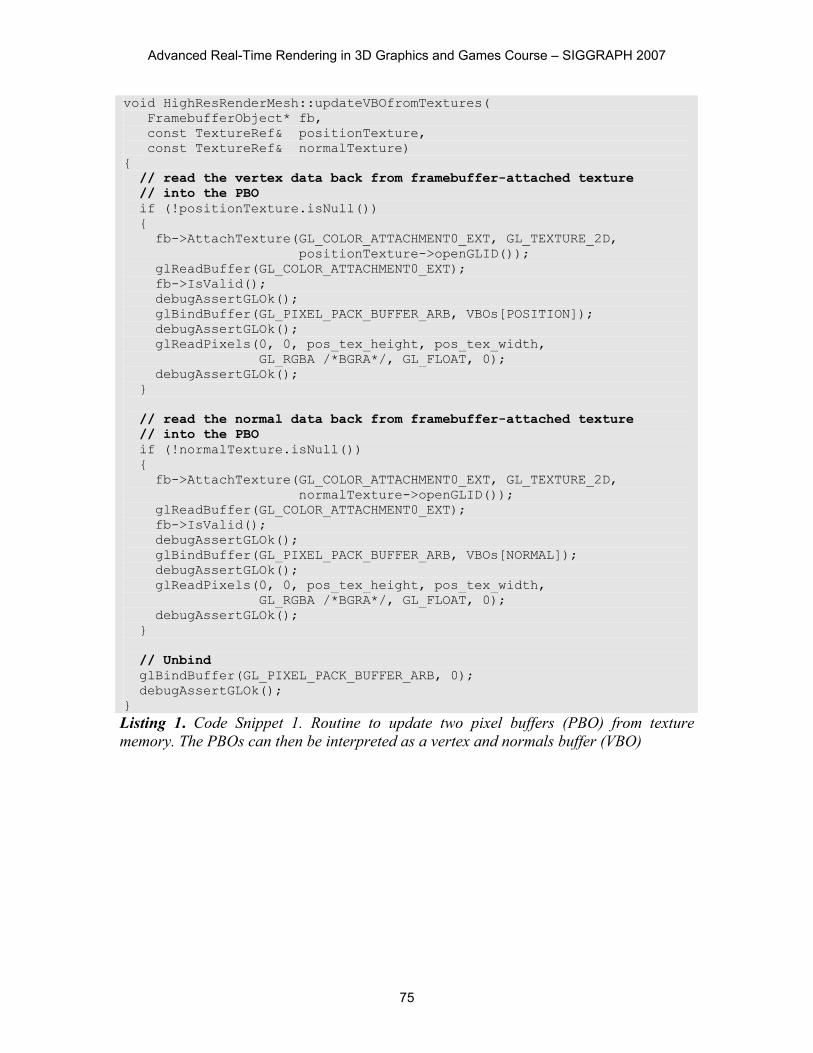
void HighResRenderMesh::updateVBOfromTextures( FramebufferObject* fb, const TextureRef& positionTexture, const TextureRef& normalTexture) { // read the vertex data back from framebuffer-attached texture // into the PBO if (!positionTexture.isNull()) { fb->AttachTexture(GL_COLOR_ATTACHMENT0_EXT, GL_TEXTURE_2D, positionTexture->openGLID()); glReadBuffer(GL_COLOR_ATTACHMENT0_EXT); fb->IsValid(); debugAssertGLOk(); glBindBuffer(GL_PIXEL_PACK_BUFFER_ARB, VBOs[POSITION]); debugAssertGLOk(); glReadPixels(0, 0, pos_tex_height, pos_tex_width, GL_RGBA /*BGRA*/, GL_FLOAT, 0); debugAssertGLOk(); } // read the normal data back from framebuffer-attached texture // into the PBO if (!normalTexture.isNull()) { fb->AttachTexture(GL_COLOR_ATTACHMENT0_EXT, GL_TEXTURE_2D, normalTexture->openGLID()); glReadBuffer(GL_COLOR_ATTACHMENT0_EXT); fb->IsValid(); debugAssertGLOk(); glBindBuffer(GL_PIXEL_PACK_BUFFER_ARB, VBOs[NORMAL]); debugAssertGLOk(); glReadPixels(0, 0, pos_tex_height, pos_tex_width, GL_RGBA /*BGRA*/, GL_FLOAT, 0); debugAssertGLOk(); } // Unbind glBindBuffer(GL_PIXEL_PACK_BUFFER_ARB, 0); debugAssertGLOk(); } Listing 1. Code Snippet 1. Routine to update two pixel buffers (PBO) from texture memory. The PBOs can then be interpreted as a vertex and normals buffer (VBO)


76

/** * Compute sparse Kx product. Does *not* write alpha. * * @param x x, an RGB(A) texture * @param y y, result buffer, an RGB(A) buffer * @param tempbuffer z, tempbuffer, should match the format of y * (default RGBA) */ template <typename model_type> void compute_sparse_product( model_type& model, texture_pointer* A, texture_pointer x, texture_pointer y, texture_pointer tempbuffer) { shared_ptr<GPUOps> gpu = model.m_gpu; shared_ptr<FramebufferObject> fbo = gpu->get_fbo(); // Update the boundary information model.m_boundaryops->update_boundaries(model, x); DebugTexture(fbo, x); if (!tempbuffer) tempbuffer = gpu->m_tempbuffer2; // First pass, 3 neighbors and self tempbuffer->Attach(get_pointer(fbo), GL_COLOR_ATTACHMENT0_EXT); gpu->Ax1->SetTextureParameter("A00", A[0]->Texture()); gpu->Ax1->SetTextureParameter("A01", A[1]->Texture()); gpu->Ax1->SetTextureParameter("A02", A[2]->Texture()); gpu->Ax1->SetTextureParameter("A20", A[3]->Texture()); gpu->Ax1->SetTextureParameter("A21", A[4]->Texture()); gpu->Ax1->SetTextureParameter("A22", A[5]->Texture()); gpu->Ax1->SetTextureParameter("A30", A[6]->Texture()); gpu->Ax1->SetTextureParameter("A31", A[7]->Texture()); gpu->Ax1->SetTextureParameter("A32", A[8]->Texture()); gpu->Ax1->SetTextureParameter("A80", A[18]->Texture()); gpu->Ax1->SetTextureParameter("A81", A[19]->Texture()); gpu->Ax1->SetTextureParameter("A82", A[20]->Texture()); gpu->Ax1->SetTextureParameter("x", x->Texture()); gpu->Ax1->SetMesh(model.GetParameterizedMesh()); gpu->Ax1->Compute(); tempbuffer->FastUnAttach(); // Second pass, 3 neighbors and tempself y->Attach(get_pointer(fbo), GL_COLOR_ATTACHMENT0_EXT); gpu->Ax2->SetTextureParameter("A40", A[9]->Texture()); gpu->Ax2->SetTextureParameter("A41", A[10]->Texture()); gpu->Ax2->SetTextureParameter("A42", A[11]->Texture()); gpu->Ax2->SetTextureParameter("A60", A[12]->Texture()); gpu->Ax2->SetTextureParameter("A61", A[13]->Texture()); gpu->Ax2->SetTextureParameter("A62", A[14]->Texture()); gpu->Ax2->SetTextureParameter("A70", A[15]->Texture()); gpu->Ax2->SetTextureParameter("A71", A[16]->Texture()); gpu->Ax2->SetTextureParameter("A72", A[17]->Texture()); gpu->Ax2->SetTextureParameter("x", x->Texture());


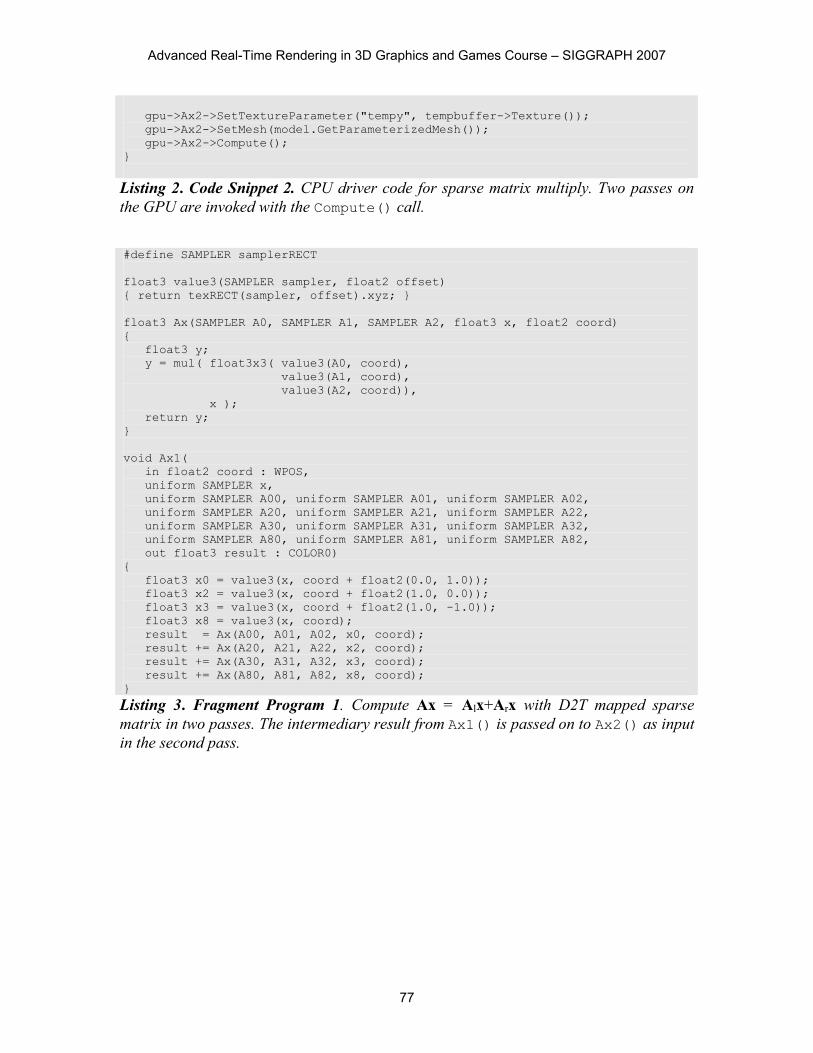
77

gpu->Ax2->SetTextureParameter("tempy", tempbuffer->Texture()); gpu->Ax2->SetMesh(model.GetParameterizedMesh()); gpu->Ax2->Compute(); } Listing 2. Code Snippet 2. CPU driver code for sparse matrix multiply. Two passes on the GPU are invoked with the Compute() call. #define SAMPLER samplerRECT float3 value3(SAMPLER sampler, float2 offset) { return texRECT(sampler, offset).xyz; } float3 Ax(SAMPLER A0, SAMPLER A1, SAMPLER A2, float3 x, float2 coord) { float3 y; y = mul( float3x3( value3(A0, coord), value3(A1, coord), value3(A2, coord)), x ); return y; } void Ax1( in float2 coord : WPOS, uniform SAMPLER x, uniform SAMPLER A00, uniform SAMPLER A01, uniform SAMPLER A02, uniform SAMPLER A20, uniform SAMPLER A21, uniform SAMPLER A22, uniform SAMPLER A30, uniform SAMPLER A31, uniform SAMPLER A32, uniform SAMPLER A80, uniform SAMPLER A81, uniform SAMPLER A82, out float3 result : COLOR0) { float3 x0 = value3(x, coord + float2(0.0, 1.0)); float3 x2 = value3(x, coord + float2(1.0, 0.0)); float3 x3 = value3(x, coord + float2(1.0, -1.0)); float3 x8 = value3(x, coord); result = Ax(A00, A01, A02, x0, coord); result += Ax(A20, A21, A22, x2, coord); result += Ax(A30, A31, A32, x3, coord); result += Ax(A80, A81, A82, x8, coord); }

Listing 3. Fragment Program 1. Compute Ax = Alx+Arx with D2T mapped sparse matrix in two passes. The intermediary result from Ax1() is passed on to Ax2() as input in the second pass.


78

void Ax2( in float2 coord : WPOS, uniform SAMPLER x, uniform SAMPLER tempy, uniform SAMPLER A40, uniform SAMPLER A41, uniform SAMPLER A42, uniform SAMPLER A60, uniform SAMPLER A61, uniform SAMPLER A62, uniform SAMPLER A70, uniform SAMPLER A71, uniform SAMPLER A72, out float3 result : COLOR0) { float3 x4 = value3(x, coord + float2(0.0, -1.0)); float3 x6 = value3(x, coord + float2(-1.0, 0.0)); float3 x7 = value3(x, coord + float2(-1.0, 1.0)); result = value3(tempy, coord); result += Ax(A40, A41, A42, x4, coord); result += Ax(A60, A61, A62, x6, coord); result += Ax(A70, A71, A72, x7, coord); }

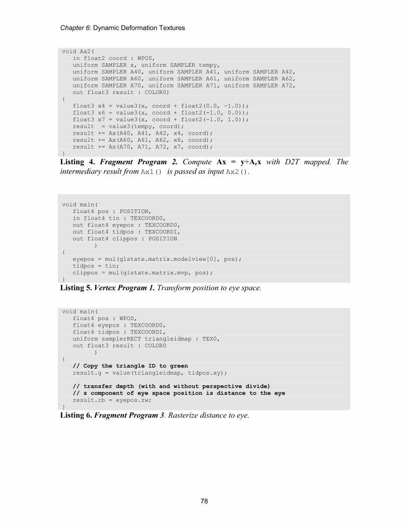
Listing 4. Fragment Program 2. Compute Ax = y+Arx with D2T mapped. The intermediary result from Ax1() is passed as input Ax2(). void main( float4 pos : POSITION, in float4 tin : TEXCOORD0, out float4 eyepos : TEXCOORD0, out float4 tidpos : TEXCOORD1, out float4 clippos : POSITION ) { eyepos = mul(glstate.matrix.modelview[0], pos); tidpos = tin; clippos = mul(glstate.matrix.mvp, pos); }

Listing 5. Vertex Program 1. Transform position to eye space. void main( float4 pos : WPOS, float4 eyepos : TEXCOORD0, float4 tidpos : TEXCOORD1, uniform samplerRECT triangleidmap : TEX0, out float3 result : COLOR0 ) { // Copy the triangle ID to green result.g = value(triangleidmap, tidpos.xy); // transfer depth (with and without perspective divide) // z component of eye space position is distance to the eye result.rb = eyepos.zw; }

Listing 6. Fragment Program 3. Rasterize distance to eye.


79

void main( in float2 coord : WPOS, uniform samplerRECT texture1, uniform samplerRECT texture2) { // Subtract texture values and copy to red float2 val1 = f2texRECT(texture1, coord.xy); float2 val2 = f2texRECT(texture2, coord.xy); result.r = val1.r - val2.r; //Copy triangle ID to green and blue result.g = val1.g; result.b = val2.g; }

Listing 7. Fragment Program 4. Compute per-texel depth differences. void tagcontactobj1( // code for object 1 in float2 coord : WPOS, in float2 texcoord : TEXCOORD0, uniform float3 lowresnormal, uniform samplerRECT pdtexture, uniform samplerRECT trianglemap, out TYPE result : COLOR0) { float3 pd = value3(pdtexture, texcoord); float triangle_id = value(trianglemap, coord); result = 0.0; // compare triangle ID and penetration depth. // Note: the triangle ID for object 1 is stored // in the green component of pd if ((pd.r > 0.0) && (abs(pd.g - triangle_id) < 0.00001)) { //store inwards lowres normal result.xyz = lowresnormal; //store penetration depth result.a = pd.x; } else { discard; } } void tagcontactobj2( // code for object 2 in float2 coord : WPOS, in float2 texcoord : TEXCOORD0, uniform float3 lowresnormal, uniform samplerRECT pdtexture, uniform samplerRECT trianglemap, out TYPE result : COLOR0) { float3 pd = value3(pdtexture, texcoord); float triangle_id = value(trianglemap, coord); result = 0.0; // compare triangle ID and penetration depth. // Note: the triangle ID for object 2 is stored // in the blue component of pd if ((pd.r > 0.0) && (abs(pd.b - triangle_id) < 0.00001)) { //store inwards lowres normal result.xyz = lowresnormal; //store penetration depth result.a = pd.x; } else { discard; } }

Listing 8. Fragment Program 5. Tag colliding texels in the D2T by transferring the collision data from D with the appropriate mapping and with triangle checking.


80

void ContactComputePolicy::ComputePolicy(const Matrix4 & contactCamMVP) { // load contact camera matrices glMatrixMode(GL_TEXTURE); static Matrix4 bias( 0.5f, 0.0f, 0.0f, 0.5f, 0.0f, 0.5f, 0.0f, 0.5f, 0.0f, 0.0f, 0.5f, 0.5f - .000001f, 0.0f, 0.0f, 0.0f, 1.0f); glLoadMatrix(m_bias); glMultMatrix(contactCamMVP); CheckErrorsGL("Loaded contact camera matrices"); // Render into D2T atlas m_mesh->RenderNearContactToAtlas(contact->Point(m_numobj), m_normal); }

Listing 9. Code Snippet 3. Set up texture matrix for projection of contact domain to D2T atlas and render into D2T atlas. void generate_normals( in float2 coord : WPOS, uniform samplerRECT bodypos, out float3 normal : COLOR0 ) { // fetch body position from position texture float3 pos = value3(bodypos, coord); float3 up = value3(bodypos, coord + float2(0,1)) - pos; float3 down = value3(bodypos, coord + float2(0,-1)) - pos; float3 left = value3(bodypos, coord + float2(-1,0)) - pos; float3 right = value3(bodypos, coord + float2(1,0)) - pos; float3 upright = value3(bodypos, coord + float2(1,1)) - pos; float3 downright = value3(bodypos, coord + float2(1,-1)) - pos; float3 upleft = value3(bodypos, coord + float2(-1,1)) - pos; float3 downleft = value3(bodypos, coord + float2(-1,-1)) - pos; float3 norm = (float3)0; norm += normalize(cross(up, left)); norm += normalize(cross(left, down)); norm += normalize(cross(down, right)); norm += normalize(cross(right, up)); norm += normalize(cross(upright, upleft)); norm += normalize(cross(upleft, downleft)); norm += normalize(cross(downleft, downright)); norm += normalize(cross(downright, upright)); normalize(norm); normal = norm; }

Listing 10. Fragment Program 6. Generate normal map by sampling of each D2T texel neighborhood.

Documents

Chapter6-Galoppo-Dynamic Deformation Texturesdeveloper.amd.com/.../02/Chapter6-Galoppo-Dynamic_Deformation_… · We have implemented this parallel implicit contact resolution method