CHAPTER7 · antenna pattern synthesis can be classiﬁed into three categories. ... For a continuous source distribution, ... Since physically only sources of ﬁnite dimensions

CHAPTER7

Antenna Synthesis and Continuous Sources

7.1 INTRODUCTION

Thus far in the book we have concentrated primarily on the analysis and design ofantennas. In the analysis problem an antenna model is chosen, and it is analyzedfor its radiation characteristics (pattern, directivity, impedance, beamwidth, efficiency,polarization, and bandwidth). This is usually accomplished by initially specifying thecurrent distribution of the antenna, and then analyzing it using standard procedures. Ifthe antenna current is not known, it can usually be determined from integral equationformulations. Numerical techniques, such as the Moment Method of Chapter 8, can beused to numerically solve the integral equations.

In practice, it is often necessary to design an antenna system that will yield desiredradiation characteristics. For example, a very common request is to design an antennawhose far-field pattern possesses nulls in certain directions. Other common requestsare for the pattern to exhibit a desired distribution, narrow beamwidth and low side-lobes, decaying minor lobes, and so forth. The task, in general, is to find not only theantenna configuration but also its geometrical dimensions and excitation distribution.The designed system should yield, either exactly or approximately, an acceptable radi-ation pattern, and it should satisfy other system constraints. This method of design isusually referred to as synthesis. Although synthesis, in its broadest definition, usuallyrefers to antenna pattern synthesis, it is often used interchangeably with design. Sincedesign methods have been outlined and illustrated previously, as in Chapter 6, in thischapter we want to introduce and illustrate antenna pattern synthesis methods.

Antenna pattern synthesis usually requires that first an approximate analytical modelis chosen to represent, either exactly or approximately, the desired pattern. The secondstep is to match the analytical model to a physical antenna model. Generally speaking,antenna pattern synthesis can be classified into three categories. One group requiresthat the antenna patterns possess nulls in desired directions. The method introducedby Schelkunoff [1] can be used to accomplish this; it will be discussed in Section 7.3.Another category requires that the patterns exhibit a desired distribution in the entirevisible region. This is referred to as beam shaping, and it can be accomplished usingthe Fourier transform [2] and the Woodward-Lawson [3], [4] methods. They will be

Antenna Theory: Analysis Design, Third Edition, by Constantine A. BalanisISBN 0-471-66782-X Copyright 2005 John Wiley & Sons, Inc.

385

386 ANTENNA SYNTHESIS AND CONTINUOUS SOURCES

discussed and illustrated in Sections 7.4 and 7.5, respectively. A third group includestechniques that produce patterns with narrow beams and low sidelobes. Some meth-ods that accomplish this have already been discussed; namely the binomial method(Section 6.8.2) and the Dolph-Tschebyscheff method (also spelled Tchebyscheff orChebyshev) of Section 6.8.3. Other techniques that belong to this family are the Tay-lor line-source (Tschebyscheff-error) [5] and the Taylor line-source (one parameter) [6].They will be outlined and illustrated in Sections 7.6 and 7.7, respectively.

The synthesis methods will be utilized to design line-sources and linear arrays whosespace factors [as defined by (4-58a)] and array factors [as defined by (6-52)] will yielddesired far-field radiation patterns. The total pattern is formed by multiplying the spacefactor (or array factor) by the element factor (or element pattern) as dictated by (4-59)[or (6-5)]. For very narrow beam patterns, the total pattern is nearly the same as thespace factor or array factor. This is demonstrated by the dipole antenna (l � λ) ofFigure 4.3 whose element factor, as given by (4-58a), is sin θ ; for values of θ near90◦(θ 90◦), sin θ 1.

The synthesis techniques will be followed with a brief discussion of some verypopular line-source distributions (triangular, cosine, cosine-squared) and continuousaperture distributions (rectangular and circular).

7.2 CONTINUOUS SOURCES

Very long (in terms of a wavelength) arrays of discrete elements usually are moredifficult to implement, more costly, and have narrower bandwidths. For such applica-tions, antennas with continuous distributions would be convenient to use. A very longwire and a large reflector represent, respectively, antennas with continuous line andaperture distributions. Continuous distribution antennas usually have larger sidelobes,are more difficult to scan, and in general, they are not as versatile as arrays of discreteelements. The characteristics of continuously distributed sources can be approximatedby discrete-element arrays, and vice-versa, and their development follows and parallelsthat of discrete-element arrays.

7.2.1 Line-Source

Continuous line-source distributions are functions of only one coordinate, and they canbe used to approximate linear arrays of discrete elements and vice-versa.

The array factor of a discrete-element array, placed along the z-axis, is given by(6-52) and (6-52a). As the number of elements increases in a fixed-length array, thesource approaches a continuous distribution. In the limit, the array factor summationreduces to an integral. For a continuous distribution, the factor that corresponds to thearray factor is known as the space factor. For a line-source distribution of length l

placed symmetrically along the z-axis as shown in Figure 7.1(a), the space factor (SF)is given by

SF(θ) =∫ +l/2

−l/2In(z

′)ej [kz′ cos θ+φn(z′)] dz′ (7-1)

where In(z′) and φn(z′) represent, respectively, the amplitude and phase distributions

along the source. For a uniform phase distribution φn(z′) = 0.

CONTINUOUS SOURCES 387

Figure 7.1 Continuous and discrete linear sources.

Equation (7-1) is a finite one-dimensional Fourier transform relating the far-fieldpattern of the source to its excitation distribution. Two-dimensional Fourier transformsare used to represent the space factors for two-dimensional source distributions. Theserelations are results of the angular spectrum concept for plane waves, introduced firstby Booker and Clemmow [2], and it relates the angular spectrum of a wave to theexcitation distribution of the source.

For a continuous source distribution, the total field is given by the product ofthe element and space factors as defined in (4-59). This is analogous to the patternmultiplication of (6-5) for arrays. The type of current and its direction of flow on asource determine the element factor. For a finite length linear dipole, for example, thetotal field of (4-58a) is obtained by summing the contributions of small infinitesimalelements which are used to represent the entire dipole. In the limit, as the infinitesimallengths become very small, the summation reduces to an integration. In (4-58a), thefactor outside the brackets is the element factor and the one within the brackets is thespace factor and corresponds to (7-1).

7.2.2 Discretization of Continuous Sources

The radiation characteristics of continuous sources can be approximated by discrete-element arrays, and vice-versa. This is illustrated in Figure 7.1(b) whereby discreteelements, with a spacing d between them, are placed along the length of the contin-uous source. Smaller spacings between the elements yield better approximations, andthey can even capture the fine details of the continuous distribution radiation char-acteristics. For example, the continuous line-source distribution In(z

′) of (7-1) canbe approximated by a discrete-element array whose element excitation coefficients, atthe specified element positions within −l/2 ≤ z′ ≤ l/2, are determined by the sam-pling of In(z′)ejφn(z

′). The radiation pattern of the digitized discrete-element array willapproximate the pattern of the continuous source.


The technique can be used for the discretization of any continuous distribution.The accuracy increases as the element spacing decreases; in the limit, the two pat-terns will be identical. For large element spacing, the patterns of the two anten-nas will not match well. To avoid this, another method known as root-matchingcan be used [7]. Instead of sampling the continuous current distribution to deter-mine the element excitation coefficients, the root-matching method requires that thenulls of the continuous distribution pattern also appear in the initial pattern of thediscrete-element array. If the synthesized pattern using this method still does notyield (within an acceptable accuracy) the desired pattern, a perturbation technique [7]can then be applied to the distribution of the discrete-element array to improve itsaccuracy.

7.3 SCHELKUNOFF POLYNOMIAL METHOD

A method that is conducive to the synthesis of arrays whose patterns possess nulls indesired directions is that introduced by Schelkunoff [1]. To complete the design, thismethod requires information on the number of nulls and their locations. The number ofelements and their excitation coefficients are then derived. The analytical formulationof the technique follows.

Referring to Figure 6.5(a), the array factor for an N -element, equally spaced, nonuni-form amplitude, and progressive phase excitation is given by (6-52) as

AF =N∑n=1

anej(n−1)(kd cos θ+β) =

N∑n=1

anej(n−1)ψ (7-2)

where an accounts for the nonuniform amplitude excitation of each element. The spac-ing between the elements is d and β is the progressive phase shift.

Lettingz = x + jy = ejψ = ej(kd cos θ+β) (7-3)

we can rewrite (7-2) as

AF =N∑n=1

anzn−1 = a1 + a2z+ a3z

2 + · · · + aNzN−1 (7-4)

which is a polynomial of degree (N − 1). From the mathematics of complex variablesand algebra, any polynomial of degree (N − 1) has (N − 1) roots and can be expressedas a product of (N − 1) linear terms. Thus we can write (7-4) as

AF = an(z− z1)(z − z2)(z − z3) · · · (z − zN−1) (7-5)

where z1, z2, z3, . . . , zN−1 are the roots, which may be complex, of the polynomial.The magnitude of (7-5) can be expressed as

|AF| = |an||z− z1||z− z2||z− z3| · · · |z− zN−1| (7-6)

SCHELKUNOFF POLYNOMIAL METHOD 389

Some very interesting observations can be drawn from (7-6) which can be used judi-ciously for the analysis and synthesis of arrays. Before tackling that phase of theproblem, let us first return and examine the properties of (7-3).

The complex variable z of (7-3) can be written in another form as

z = |z|ejψ = |z| � ψ = 1 � ψ (7-7)

ψ = kd cos θ + β = 2π

λd cos θ + β (7-7a)

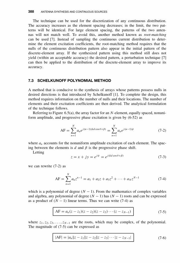
It is clear that for any value of d, θ , or β the magnitude of z lies always on a unitcircle; however its phase depends upon d, θ , and β. For β = 0, we have plotted inFigures 7-2(a)–(d) the value of z, magnitude and phase, as θ takes values of 0 to π

rad. It is observed that for d = λ/8 the values of z, for all the physically observable

Figure 7.2 V isible Region (VR) and Invisible Region (IR) boundaries for complex variablez when β = 0.


angles of θ , only exist over the part of the circle shown in Figure 7.2(a). Any valuesof z outside that arc are not realizable by any physical observation angle θ for thespacing d = λ/8. We refer to the realizable part of the circle as the visible region andthe remaining as the invisible region. In Figure 7.2(a) we also observe the path of thez values as θ changes from 0◦ to 180◦.

In Figures 7.2(b)–(d) we have plotted the values of z when the spacing between theelements is λ/4, λ/2, and 3λ/4. It is obvious that the visible region can be extendedby increasing the spacing between the elements. It requires a spacing of at least λ/2to encompass, at least once, the entire circle. Any spacing greater than λ/2 leads tomultiple values for z. In Figure 7.2(d) we have double values for z for half of thecircle when d = 3λ/4.

To demonstrate the versatility of the arrays, in Figures 7.3(a)–(d) we have plottedthe values of z for the same spacings as in Figure 7.2(a)–(d) but with a β = π/4. A

2

2

Figure 7.3 V isible Region (VR) and Invisible Region (IR) boundaries for complex variablez when β = π/4.

SCHELKUNOFF POLYNOMIAL METHOD 391

comparison between the corresponding figures indicates that the overall visible regionfor each spacing has not changed but its relative position on the unit circle has rotatedcounterclockwise by an amount equal to β.

We can conclude then that the overall extent of the visible region can be controlledby the spacing between the elements and its relative position on the unit circle by theprogressive phase excitation of the elements. These two can be used effectively in thedesign of the array factors.

Now let us return to (7-6). The magnitude of the array factor, its form as shownin (7-6), has a geometrical interpretation. For a given value of z in the visible regionof the unit circle, corresponding to a value of θ as determined by (7-3), |AF| isproportional to the product of the distances between z and z1, z2, z3, . . . , zN−1, theroots of AF. In addition, apart from a constant, the phase of AF is equal to the sumof the phases between z and each of the zeros (roots). This is best demonstratedgeometrically in Figure 7.4(a). If all the roots z1, z2, z3, . . . , zN−1 are located in thevisible region of the unit circle, then each one corresponds to a null in the patternof |AF| because as θ changes z changes and eventually passes through each of thezn’s. When it does, the length between z and that zn is zero and (7-6) vanishes.When all the zeros (roots) are not in the visible region of the unit circle, but somelie outside it and/or any other point not on the unit circle, then only those zeroson the visible region will contribute to the nulls of the pattern. This is shown geo-metrically in Figure 7.4(b). If no zeros exist in the visible region of the unit circle,then that particular array factor has no nulls for any value of θ . However, if a givenzero lies on the unit circle but not in its visible region, that zero can be included inthe pattern by changing the phase excitation β so that the visible region is rotateduntil it encompasses that root. Doing this, and not changing d , may exclude someother zero(s).

To demonstrate all the principles, we will consider an example along with somecomputations.

Figure 7.4 Array factor roots within and outside unit circle, and visible and invisible regions.


Example 7.1

Design a linear array with a spacing between the elements of d = λ/4 such that it has zerosat θ = 0◦, 90◦, and 180◦. Determine the number of elements, their excitation, and plot thederived pattern. Use Schelkunoff’s method.

Solution: For a spacing of λ/4 between the elements and a phase shift β = 0◦, the visibleregion is shown in Figure 7.2(b). If the desired zeros of the array factor must occur atθ = 0◦, 90◦, and 180◦, then these correspond to z = j, 1,−j on the unit circle. Thus anormalized form of the array factor is given by

AF = (z − z1)(z − z2)(z− z3) = (z − j)(z − 1)(z+ j)

AF = z3 − z2 + z− 1

Figure 7.5 Amplitude radiation pattern of a four-element array of isotropic sources with aspacing of λ/4 between them, zero degrees progressive phase shift, and zeros at θ = 0◦, 90◦,and 180◦.

FOURIER TRANSFORM METHOD 393

Referring to (7-4), the above array factor and the desired radiation characteristics can berealized when there are four elements and their excitation coefficients are equal to

a1 = −1

a2 = +1

a3 = −1

a4 = +1

To illustrate the method, we plotted in Figure 7.5 the pattern of that array; it clearlymeets the desired specifications. Because of the symmetry of the array, the pattern of theleft hemisphere is identical to that of the right.

7.4 FOURIER TRANSFORM METHOD

This method can be used to determine, given a complete description of the desiredpattern, the excitation distribution of a continuous or a discrete source antenna system.The derived excitation will yield, either exactly or approximately, the desired antennapattern. The pattern synthesis using this method is referred to as beam shaping.

7.4.1 Line-Source

For a continuous line-source distribution of length l, as shown in Figure 7.1, the nor-malized space factor of (7-1) can be written as

SF(θ) =∫ l/2

−l/2I (z′)ej (k cos θ−kz)z′ dz′ =

∫ l/2

−l/2I (z′)ejξz

′dz′ (7-8)

ξ = k cos θ − kz ➱ θ = cos−1

(ξ + kz

k

)(7-8a)

where kz is the excitation phase constant of the source. For a normalized uniformcurrent distribution of the form I (z′) = I0/l, (7-8) reduces to

SF(θ) = I0

sin

[kl

2

(cos θ − kz

k

)]kl

2

(cos θ − kz

k

) (7-9)

The observation angle θ of (7-9) will have real values (visible region) provided that−(k + kz) ≤ ξ ≤ (k − kz) as obtained from (7-8a).

Since the current distribution of (7-8) extends only over −l/2 ≤ z′ ≤ l/2 (and it iszero outside it), the limits can be extended to infinity and (7-8) can be written as

SF(θ) = SF(ξ) =∫ +∞

−∞I (z′)ejξz

′dz′ (7-10a)


The form of (7-10a) is a Fourier transform, and it relates the excitation distributionI (z′) of a continuous source to its far-field space factor SF(θ). The transform pair of(7-10a) is given by

I (z′) = 1

2π

∫ +∞

−∞SF(ξ)e−jz

′ξ dξ = 1

2π

∫ +∞

−∞SF(θ)e−jz

′ξ dξ (7-10b)

Whether (7-10a) represents the direct transform and (7-10b) the inverse transform,or vice-versa, does not matter here. The most important thing is that the excitationdistribution and the far-field space factor are related by Fourier transforms.

Equation (7-10b) indicates that if SF(θ) represents the desired pattern, the excitationdistribution I (z′) that will yield the exact desired pattern must in general exist forall values of z′(−∞ ≤ z′ ≤ ∞). Since physically only sources of finite dimensionsare realizable, the excitation distribution of (7-10b) is usually truncated at z′ = ±l/2(beyond z′ = ±l/2 it is set to zero). Thus the approximate source distribution is givenby

Ia(z′)

I (z

′) = 1

2π

∫ +∞

−∞SF(ξ)e−jz

′ξ dξ −l/2 ≤ z′ ≤ l/2

0 elsewhere(7-11)

and it yields an approximate pattern SF(θ)a . The approximate pattern is used to rep-resent, within certain error, the desired pattern SF(θ)d . Thus

SF(θ)d SF(θ)a =∫ l/2

−l/2Ia(z

′)ejξz′dz′ (7-12)

It can be shown that, over all values of ξ , the synthesized approximate patternSF(θ)a yields the least-mean-square error or deviation from the desired pattern SF(θ)d .However that criterion is not satisfied when the values of ξ are restricted only in thevisible region [8], [9].

To illustrate the principles of this design method, an example is taken.

Example 7.2

Determine the current distribution and the approximate radiation pattern of a line-sourceplaced along the z-axis whose desired radiation pattern is symmetrical about θ = π/2, andit is given by

SF(θ) ={

1 π/4 ≤ θ ≤ 3π/40 elsewhere

This is referred to as a sectoral pattern, and it is widely used in radar search and communi-cation applications.


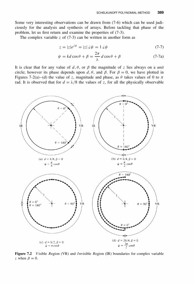
Solution: Since the pattern is symmetrical, kz = 0. The values of ξ , as determined by(7-8a), are given by k/

√2 ≥ ξ ≥ −k/√2. In turn, the current distribution is given by (7-

10b) or

I (z′) = 1

2π

∫ +∞

−∞SF(ξ)e−jz

′ξ dξ

= 1

2π

∫ k/√

2

−k/√2e−jz

′ξ dξ = k

π√

2

sin

(kz′√

2

)kz′√

2

Figure 7.6 Normalized current distribution, desired pattern, and synthesized patterns usingthe Fourier transform method.


and it exists over all values of z′(−∞ ≤ z′ ≤ ∞). Over the extent of the line-source, thecurrent distribution is approximated by

Ia(z′) I (z′), −l/2 ≤ z′ ≤ l/2

If the derived current distribution I (z′) is used in conjunction with (7-10a) and it is assumedto exist over all values of z′, the exact and desired sectoral pattern will result. If howeverit is truncated at z′ = ±l/2 (and assumed to be zero outside), then the desired pattern isapproximated by (7-12) or

SF(θ)d SF(θ)a =∫ l/2

−l/2Ia(z

′)ejξz′dz′

= 1

π

{Si

[l

λπ

(cos θ + 1√

2

)]− Si

[l

λπ

(cos θ − 1√

2

)]}

where Si(x) is the sine integral of (4-68b).The approximate current distribution (normalized so that its maximum is unity) is plotted

in Figure 7.6(a) for l = 5λ and l = 10λ. The corresponding approximate normalized patternsare shown in Figure 7.6(b) where they are compared with the desired pattern. A very goodreconstruction is indicated. The longer line-source (l = 10λ) provides a better realization.The sidelobes are about 0.102 (−19.83 dB) for l = 5λ and 0.081 (−21.83 dB) for l = 10λ(relative to the pattern at θ = 90◦).

7.4.2 Linear Array

The array factor of an N -element linear array of equally spaced elements and nonuni-form excitation is given by (7-2). If the reference point is taken at the physical centerof the array, the array factor can also be written as

Odd Number of Elements (N = 2M + 1)

AF(θ) = AF(ψ) =M∑

m=−Mame

jmψ(7-13a)

Even Number of Elements (N = 2M)

AF(θ) = AF(ψ) =−1∑

m=−Mame

j [(2m+1)/2]ψ +M∑m=1

amej [(2m−1)/2]ψ

(7-13b)

where

ψ = kd cos θ + β (7-13c)


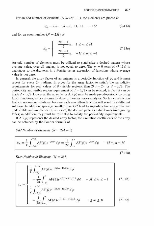
For an odd number of elements (N = 2M + 1), the elements are placed at

z′m = md, m = 0,±1,±2, . . . ,±M (7-13d)

and for an even number (N = 2M) at

z′m =

2m− 1

2d, 1 ≤ m ≤ M

2m+ 1

2d, −M ≤ m ≤ −1

(7-13e)

An odd number of elements must be utilized to synthesize a desired pattern whoseaverage value, over all angles, is not equal to zero. The m = 0 term of (7-13a) isanalogous to the d.c. term in a Fourier series expansion of functions whose averagevalue is not zero.

In general, the array factor of an antenna is a periodic function of ψ , and it mustrepeat for every 2π radians. In order for the array factor to satisfy the periodicityrequirements for real values of θ (visible region), then 2kd = 2π or d = λ/2. Theperiodicity and visible region requirement of d = λ/2 can be relaxed; in fact, it can bemade d < λ/2. However, the array factor AF(ψ) must be made pseudoperiodic by usingfill-in functions, as is customarily done in Fourier series analysis. Such a constructionleads to nonunique solutions, because each new fill-in function will result in a differentsolution. In addition, spacings smaller than λ/2 lead to superdirective arrays that areundesirable and impractical. If d > λ/2, the derived patterns exhibit undesired gratinglobes; in addition, they must be restricted to satisfy the periodicity requirements.

If AF(ψ) represents the desired array factor, the excitation coefficients of the arraycan be obtained by the Fourier formula of

Odd Number of Elements (N = 2M + 1)

am = 1

T

∫ T/2

−T/2AF(ψ)e−jmψ dψ = 1

2π

∫ π

−πAF(ψ)e−jmψ dψ −M ≤ m ≤ M

(7-14a)Even Number of Elements (N = 2M)

am =

1

T

∫ T/2

−T/2AF(ψ)e−j [(2m+1)/2]ψ dψ

= 1

2π

∫ π

−πAF(ψ)e−j [(2m+1)/2]ψ dψ −M ≤ m ≤ −1

1

T

∫ T/2

−T/2AF(ψ)e−j [(2m−1)/2]ψ dψ

= 1

2π

∫ π

−πAF(ψ)e−j [(2m−1)/2]ψ dψ 1 ≤ m ≤ M

(7-14b)

(7-14c)


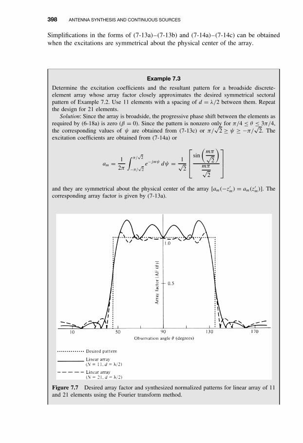
Simplifications in the forms of (7-13a)–(7-13b) and (7-14a)–(7-14c) can be obtainedwhen the excitations are symmetrical about the physical center of the array.

Example 7.3

Determine the excitation coefficients and the resultant pattern for a broadside discrete-element array whose array factor closely approximates the desired symmetrical sectoralpattern of Example 7.2. Use 11 elements with a spacing of d = λ/2 between them. Repeatthe design for 21 elements.

Solution: Since the array is broadside, the progressive phase shift between the elements asrequired by (6-18a) is zero (β = 0). Since the pattern is nonzero only for π/4 ≤ θ ≤ 3π/4,the corresponding values of ψ are obtained from (7-13c) or π/

√2 ≥ ψ ≥ −π/√2. The

excitation coefficients are obtained from (7-14a) or

am = 1

2π

∫ π/√

2

−π/√2e−jmψ dψ = 1√

2

sin

(mπ√

2

)mπ√

2

and they are symmetrical about the physical center of the array [am(−z′m) = am(z′m)]. The

corresponding array factor is given by (7-13a).

Figure 7.7 Desired array factor and synthesized normalized patterns for linear array of 11and 21 elements using the Fourier transform method.

WOODWARD-LAWSON METHOD 399

The normalized excitation coefficients are

a0 = 1.0000 a±4 = 0.0578 a±8 = −0.0496a±1 = 0.3582 a±5 = −0.0895 a±9 = 0.0455a±2 = −0.2170 a±6 = 0.0518 a±10 = −0.0100a±3 = 0.0558 a±7 = 0.0101

They are displayed graphically by a dot (ž) in Figure 7.6(a) where they are compared with thecontinuous current distribution of Example 7.2. It is apparent that at the element positions,the line-source and linear array excitation values are identical. This is expected since thetwo antennas are of the same length (for N = 11, d = λ/2 ➱ l = 5λ and for N = 21, d =λ/2 ➱ l = 10λ).

The corresponding normalized array factors are displayed in Figure 7.7. As it shouldbe expected, the larger array (N = 21, d = λ/2) provides a better reconstruction of thedesired pattern. The sidelobe levels, relative to the value of the pattern at θ = 90◦, are 0.061(−24.29 dB) for N = 11 and 0.108 (−19.33 dB) for N = 21.

Discrete-element linear arrays only approximate continuous line-sources. Therefore, theirpatterns shown in Figure 7.7 do not approximate as well the desired pattern as the corre-sponding patterns of the line-source distributions shown in Figure 7.6(b).

Whenever the desired pattern contains discontinuities or its values in a given regionchange very rapidly, the reconstruction pattern will exhibit oscillatory overshootswhich are referred to as Gibbs’ phenomena. Since the desired sectoral patterns ofExamples 7.2 and 7.3 are discontinuous at θ = π/4 and 3π/4, the reconstructed pat-terns displayed in Figures 7.6(b) and 7.7 exhibit these oscillatory overshoots.

7.5 WOODWARD-LAWSON METHOD

A very popular antenna pattern synthesis method used for beam shaping was introducedby Woodward and Lawson [3], [4], [10]. The synthesis is accomplished by samplingthe desired pattern at various discrete locations. Associated with each pattern sample isa harmonic current of uniform amplitude distribution and uniform progressive phase,whose corresponding field is referred to as a composing function. For a line-source,each composing function is of an bm sin(ψm)/ψm form whereas for a linear array ittakes an bm sin(Nφm)/N sin(φm) form. The excitation coefficient bm of each harmoniccurrent is such that its field strength is equal to the amplitude of the desired patternat its corresponding sampled point. The total excitation of the source is comprisedof a finite summation of space harmonics. The corresponding synthesized pattern isrepresented by a finite summation of composing functions with each term represent-ing the field of a current harmonic with uniform amplitude distribution and uniformprogressive phase.

The formation of the overall pattern using the Woodward-Lawson method is accom-plished as follows. The first composing function produces a pattern whose mainbeam placement is determined by the value of its uniform progressive phase whileits innermost sidelobe level is about −13.5 dB; the level of the remaining sidelobes


monotonically decreases. The second composing function has also a similar patternexcept that its uniform progressive phase is adjusted so that its main lobe maximumcoincides with the innermost null of the first composing function. This results in thefilling-in of the innermost null of the pattern of the first composing function; the amountof filling-in is controlled by the amplitude excitation of the second composing function.Similarly, the uniform progressive phase of the third composing function is adjustedso that the maximum of its main lobe occurs at the second innermost null of the firstcomposing function; it also results in filling-in of the second innermost null of thefirst composing function. This process continues with the remaining finite number ofcomposing functions.

The Woodward-Lawson method is simple, elegant, and provides insight into theprocess of pattern synthesis. However, because the pattern of each composing functionperturbs the entire pattern to be synthesized, it lacks local control over the sidelobelevel in the unshaped region of the entire pattern. In 1988 and 1989 a spirited and wel-comed dialogue developed concerning the Woodward-Lawson method [11]–[14]. Thedialogue centered whether the Woodward-Lawson method should be taught and evenappear in textbooks, and whether it should be replaced by an alternate method [15]which overcomes some of the shortcomings of the Woodward-Lawson method. Thealternate method of [15] is more of a numerical and iterative extension of Schelkunoff’spolynomial method which may be of greater practical value because it provides supe-rior beamshape and pattern control. One of the distinctions of the two methods is thatthe Woodward-Lawson method deals with the synthesis of field patterns while thatof [15] deals with the synthesis of power patterns.

The analytical formulation of this method is similar to the Shannon sampling the-orem used in communications which states that “if a function g(t) is band-limited,with its highest frequency being fh, the function g(t) can be reconstructed usingsamples taken at a frequency fs . To faithfully reproduce the original function g(t),the sampling frequency fs should be at least twice the highest frequency fh (fs ≥2fh) or the function should be sampled at points separated by no more than 3t ≤1/fs ≥ 1/(2fh) = Th/2 where Th is the period of the highest frequency fh.” In asimilar manner, the radiation pattern of an antenna can be synthesized by samplingfunctions whose samples are separated by λ/l rad, where l is the length of thesource [9], [10].

7.5.1 Line-Source

Let the current distribution of a continuous source be represented, within −l/2 ≤ z′ ≤l/2, by a finite summation of normalized sources each of constant amplitude and linearphase of the form

im(z′) = bm

le−jkz

′ cos θm − l/2 ≤ z′ ≤ l/2 (7-15)

As it will be shown later, θm represents the angles where the desired pattern is sampled.The total current I (z′) is given by a finite summation of 2M (even samples) or 2M + 1(odd samples) current sources each of the form of (7-15). Thus


I (z′) = 1

l

M∑m=−M

bme−jkz′ cos θm

(7-16)

where

m = ±1,±2, . . . ,±M (for 2M even number of samples) (7-16a)

m = 0,±1,±2, . . . ,±M (for 2M + 1 odd number of samples) (7-16b)

For simplicity use odd number of samples.Associated with each current source of (7-15) is a corresponding field pattern of the

form given by (7-9) or

sm(θ) = bm

sin

[kl

2(cos θ − cos θm)

]kl


(7-17)

whose maximum occurs when θ = θm. The total pattern is obtained by summing 2M(even samples) or 2M + 1 (odd samples) terms each of the form given by (7-17). Thus

SF(θ) =M∑

m=−Mbm

sin

[kl


]kl


(7-18)

The maximum of each individual term in (7-18) occurs when θ = θm, and it is equalto SF(θ = θm). In addition, when one term in (7-18) attains its maximum value at itssample at θ = θm, all other terms of (7-18) which are associated with the other samplesare zero at θ = θm. In other words, all sampling terms (composing functions) of (7-18)are zero at all sampling points other than at their own. Thus at each sampling point thetotal field is equal to that of the sample. This is one of the most appealing properties ofthis method. If the desired space factor is sampled at θ = θm, the excitation coefficientsbm can be made equal to its value at the sample points θm. Thus

bm = SF(θ = θm)d (7-19)

The reconstructed pattern is then given by (7-18), and it approximates closely thedesired pattern.

In order for the synthesized pattern to satisfy the periodicity requirements of 2π forreal values of θ (visible region) and to faithfully reconstruct the desired pattern, eachsample should be separated by

kz′3||z′|=l = 2π ➱3 = λ

l(7-19a)


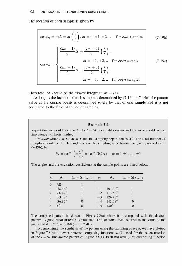
The location of each sample is given by

cos θm = m3 = m

(λ

l

), m = 0,±1,±2, .. for odd samples

cos θm =

(2m− 1)

23 = (2m− 1)

2

(λ

l

),

m = +1,+2, .. for even samples

(2m+ 1)

23 = (2m+ 1)

2

(λ

l

),

m = −1,−2, .. for even samples

(7-19b)

(7-19c)

Therefore, M should be the closest integer to M = l/λ.As long as the location of each sample is determined by (7-19b or 7-19c), the pattern

value at the sample points is determined solely by that of one sample and it is notcorrelated to the field of the other samples.

Example 7.4

Repeat the design of Example 7.2 for l = 5λ using odd samples and the Woodward-Lawsonline-source synthesis method.

Solution: Since l = 5λ,M = 5 and the sampling separation is 0.2. The total number ofsampling points is 11. The angles where the sampling is performed are given, according to(7-19b), by

θm = cos−1

(mλ

l

)= cos−1(0.2m), m = 0,±1, . . . ,±5

The angles and the excitation coefficients at the sample points are listed below.

m θm bm = SF(θm)d m θm bm = SF(θm)d

0 90◦ 11 78.46◦ 1 −1 101.54◦ 12 66.42◦ 1 −2 113.58◦ 13 53.13◦ 1 −3 126.87◦ 14 36.87◦ 0 −4 143.13◦ 05 0◦ 0 −5 180◦ 0

The computed pattern is shown in Figure 7.8(a) where it is compared with the desiredpattern. A good reconstruction is indicated. The sidelobe level, relative to the value of thepattern at θ = 90◦, is 0.160 (−15.92 dB).

To demonstrate the synthesis of the pattern using the sampling concept, we have plottedin Figure 7.8(b) all seven nonzero composing functions sm(θ) used for the reconstructionof the l = 5λ line-source pattern of Figure 7.8(a). Each nonzero sm(θ) composing function


0.5

90 135 180450

θObservation angle (degrees)

(a) Normalized amplitude patterns

Nor

mal

ized

mag

nitu

de

1.0

(b) Composing functions for line-source (l = 5 )

1.0

λ

Desired patternLine-source (l = 5 ) Composing functions sm ( ),m = 0, ±1, ±2, ±3

SF ( )θθ

λ

Desired patternLine-source (l = 5 ) Linear array (N = 10, d = /2)

SF ( )AF ( )

θθ

λλ

Figure 7.8 Desired and synthesized patterns, and composing functions for Wood-ward-Lawson designs.


was computed using (7-17) for m = 0,±1,±2,±3. It is evident that at each sampling pointall the composing functions are zero, except the one that represents that sample. Thus thevalue of the desired pattern at each sampling point is determined solely by the maximumvalue of a single composing function. The angles where the composing functions attain theirmaximum values are listed in the previous table.

7.5.2 Linear Array

The Woodward-Lawson method can also be implemented to synthesize discrete lineararrays. The technique is similar to the Woodward-Lawson method for line-sourcesexcept that the pattern of each sample, as given by (7-17), is replaced by the arrayfactor of a uniform array as given by (6-10c). The pattern of each sample can bewritten as

fm(θ) = bm

sin

[N

2kd(cos θ − cos θm)

]

N sin

[1


] (7-20)

l = Nd assumes the array is equal to the length of the line-source (for this designonly, the length l of the line includes a distance d/2 beyond each end element). Thetotal array factor can be written as a superposition of 2M + 1 sampling terms (as wasdone for the line-source) each of the form of (7-20). Thus

AF(θ) =M∑

m=−Mbm

sin

[N


]

N sin

[1


] (7-21)

As for the line-sources, the excitation coefficients of the array elements at the samplepoints are equal to the value of the desired array factor at the sample points. That is,

bm = AF(θ = θm)d (7-22)

The sample points are taken at

cos θm = m3 = m

(λ

l

), m = 0,±1,±2, .. for odd samples

cos θm =

(2m− 1)

23 = (2m− 1)

2

(λ

Nd

),

m = +1,+2, .. for even samples

(2m+ 1)

23 = (2m+ 1)

2

(λ

Nd

),

m = −1,−2, .. for even samples

(7-23a)

(7-23b)


The normalized excitation coefficient of each array element, required to give the desiredpattern, is given by

an(z′) = 1

N

M∑m=−M

bme−jkzn ′ cos θm

(7-24)

where zn′ indicates the position of the nth element (element in question) symmetricallyplaced about the geometrical center of the array.

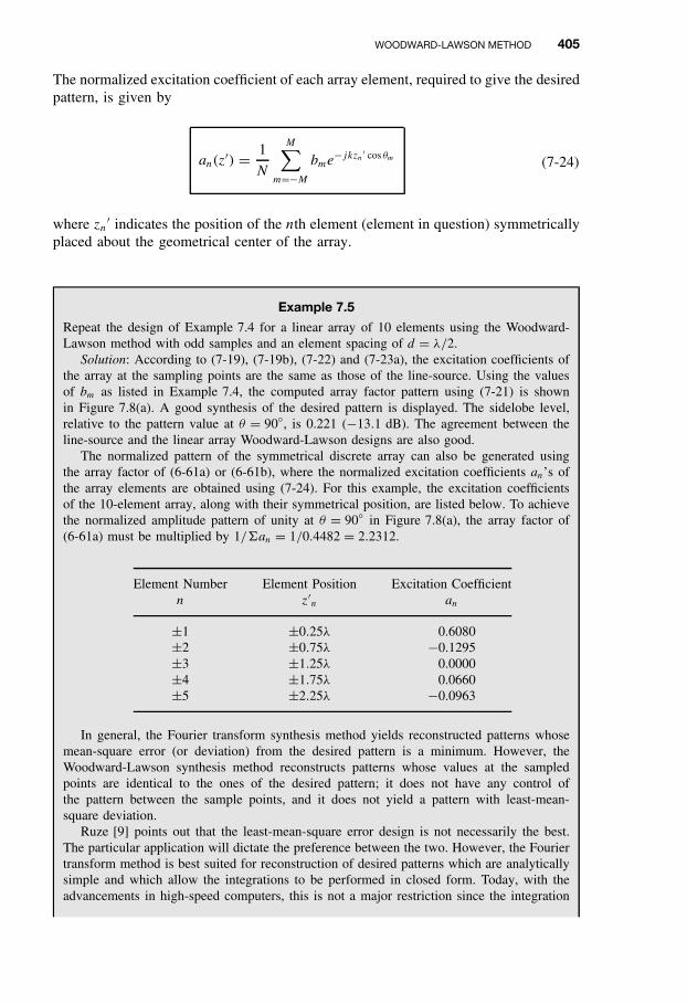
Example 7.5

Repeat the design of Example 7.4 for a linear array of 10 elements using the Woodward-Lawson method with odd samples and an element spacing of d = λ/2.

Solution: According to (7-19), (7-19b), (7-22) and (7-23a), the excitation coefficients ofthe array at the sampling points are the same as those of the line-source. Using the valuesof bm as listed in Example 7.4, the computed array factor pattern using (7-21) is shownin Figure 7.8(a). A good synthesis of the desired pattern is displayed. The sidelobe level,relative to the pattern value at θ = 90◦, is 0.221 (−13.1 dB). The agreement between theline-source and the linear array Woodward-Lawson designs are also good.

The normalized pattern of the symmetrical discrete array can also be generated usingthe array factor of (6-61a) or (6-61b), where the normalized excitation coefficients an’s ofthe array elements are obtained using (7-24). For this example, the excitation coefficientsof the 10-element array, along with their symmetrical position, are listed below. To achievethe normalized amplitude pattern of unity at θ = 90◦ in Figure 7.8(a), the array factor of(6-61a) must be multiplied by 1/�an = 1/0.4482 = 2.2312.

Element Number Element Position Excitation Coefficientn z′n an

±1 ±0.25λ 0.6080±2 ±0.75λ −0.1295±3 ±1.25λ 0.0000±4 ±1.75λ 0.0660±5 ±2.25λ −0.0963

In general, the Fourier transform synthesis method yields reconstructed patterns whosemean-square error (or deviation) from the desired pattern is a minimum. However, theWoodward-Lawson synthesis method reconstructs patterns whose values at the sampledpoints are identical to the ones of the desired pattern; it does not have any control ofthe pattern between the sample points, and it does not yield a pattern with least-mean-square deviation.

Ruze [9] points out that the least-mean-square error design is not necessarily the best.The particular application will dictate the preference between the two. However, the Fouriertransform method is best suited for reconstruction of desired patterns which are analyticallysimple and which allow the integrations to be performed in closed form. Today, with theadvancements in high-speed computers, this is not a major restriction since the integration


can be performed (with high efficiency) numerically. In contrast, the Woodward-Lawsonmethod is more flexible, and it can be used to synthesize any desired pattern. In fact, itcan even be used to reconstruct patterns which, because of their complicated nature, cannotbe expressed analytically. Measured patterns, either of analog or digital form, can also besynthesized using the Woodward-Lawson method.

7.6 TAYLOR LINE-SOURCE (TSCHEBYSCHEFF-ERROR)

In Chapter 6 we discussed the classic Dolph-Tschebyscheff array design which yields,for a given sidelobe level, the smallest possible first-null beamwidth (or the smallestpossible sidelobe level for a given first-null beamwidth). Another classic design thatis closely related to it, but is more applicable for continuous distributions, is that byTaylor [5] (this method is different from that by Taylor [6] which will be discussed inthe next section).

The Taylor design [5] yields a pattern that is an optimum compromise betweenbeamwidth and sidelobe level. In an ideal design, the minor lobes are maintained atan equal and specific level. Since the minor lobes are of equal ripple and extend toinfinity, this implies an infinite power. More realistically, however, the technique asintroduced by Taylor leads to a pattern whose first few minor lobes (closest to themain lobe) are maintained at an equal and specified level; the remaining lobes decaymonotonically. Practically, even the level of the closest minor lobes exhibits a slightmonotonic decay. This decay is a function of the space u over which these minor lobesare required to be maintained at an equal level. As this space increases, the rate ofdecay of the closest minor lobes decreases. For a very large space of u (over which theclosest minor lobes are required to have an equal ripple), the rate of decay is negligible.It should be pointed out, however, that the other method by Taylor [6] (of Section 7.7)yields minor lobes, all of which decay monotonically.

The details of the analytical formulation are somewhat complex (for the averagereader) and lengthy, and they will not be included here. The interested reader is referredto the literature [5], [16]. Instead, a succinct outline of the salient points of the methodand of the design procedure will be included. The design is for far-field patterns, andit is based on the formulation of (7-1).

Ideally the normalized space factor that yields a pattern with equal-ripple minorlobes is given by

SF(θ) = cosh[√(πA)2 − u2]

cosh(πA)(7-25)

u = πl

λcos θ (7-25a)

whose maximum value occurs when u = 0. The constant A is related to the maximumdesired sidelobe level R0 by

cosh(πA) = R0 (voltage ratio) (7-26)

TAYLOR LINE-SOURCE (TSCHEBYSCHEFF-ERROR) 407

The space factor of (7-25) can be derived from the Dolph-Tschebyscheff arrayformulation of Section 6.8.3, if the number of elements of the array are allowed tobecome infinite.

Since (7-25) is ideal and cannot be realized physically, Taylor [5] suggested that itbe approximated (within a certain error) by a space factor comprised of a product offactors whose roots are the zeros of the pattern. Because of its approximation to theideal Tschebyscheff design, it is also referred to as Tschebyscheff-error. The Taylorspace factor is given by

SF(u,A, n) = sin(u)

u

n−1∏n=1

[1−

(u

un

)2]

n−1∏n=1

[1−

( u

nπ

)2] (7-27)

u = πv = πl

λcos θ (7-27a)

un = πvn = πl

λcos θn (7-27b)

where θn represents the locations of the nulls. The parameter n is a constant chosenby the designer so that the minor lobes for |v| = |u/π | ≤ n are maintained at a nearlyconstant voltage level of 1/R0 while for |v| = |u/π | > n the envelope, through themaxima of the remaining minor lobes, decays at a rate of 1/v = π/u. In addition, thenulls of the pattern for |v| ≥ n occur at integer values of v.

In general, there are n− 1 inner nulls for |v| < n and an infinite number of outernulls for |v| ≥ n. To provide a smooth transition between the inner and the outer nulls(at the expense of slight beam broadening), Taylor introduced a parameter σ . It isusually referred to as the scaling factor, and it spaces the inner nulls so that they blendsmoothly with the outer ones. In addition, it is the factor by which the beamwidth ofthe Taylor design is greater than that of the Dolph-Tschebyscheff, and it is given by

σ = n√A2 + (n− 1

2

)2 (7-28)

The location of the nulls are obtained using

un = πvn = πl

λcos θn =

{±πσ

√A2 + (n− 1

2

)21 ≤ n < n

±nπ n ≤ n ≤ ∞(7-29)

The normalized line-source distribution, which yields the desired pattern, is given by

I (z′) = λ

l

1+ 2

n−1∑p=1

SF(p,A, n) cos

(2πp

z′

l

) (7-30)


The coefficients SF(p,A, n) represent samples of the Taylor pattern, and they canbe obtained from (7-27) with u = πp. They can also be found using

SF(p,A, n) =

[(n− 1)!]2

(n− 1+ p)!(n− 1− p)!

n−1∏m=1

[1−

(πp

um

)2]

|p| < n

0 |p| ≥ n

(7-30a)

with SF(−p,A, n) = SF(p,A, n).The half-power beamwidth is given approximately by [8]

40 2 sin−1

λσπl

[(cosh−1R0)

2 −(

cosh−1 R0√2

)2]1/2

(7-31)

7.6.1 Design Procedure

To initiate a Taylor design, you must

1. specify the normalized maximum tolerable sidelobe level 1/R0 of the pattern.2. choose a positive integer value for n such that for |v| = |(l/λ) cos θ | ≤ n the

normalized level of the minor lobes is nearly constant at 1/R0. For |v| > n, theminor lobes decrease monotonically. In addition, for |v| < n there exist (n− 1)nulls. The position of all the nulls is found using (7-29). Small values of n yieldsource distributions which are maximum at the center and monotonically decreasetoward the edges. In contrast, large values of n result in sources which are peakedsimultaneously at the center and at the edges, and they yield sharper main beams.Therefore, very small and very large values of n should be avoided. Typically,the value of n should be at least 3 and at least 6 for designs with sidelobes of−25 and −40 dB, respectively.

To complete the design, you do the following:

1. Determine A using (7-26), σ using (7-28), and the nulls using (7-29).2. Compute the space factor using (7-27), the source distribution using (7-30) and

(7-30a), and the half-power beamwidth using (7-31).

Example 7.6

Design a −20 dB Taylor, Tschebyscheff-error, distribution line-source with n = 5. Plot thepattern and the current distribution for l = 7λ(−7 ≤ v = u/π ≤ 7).

Solution: For a −20 dB sidelobe level

R0 (voltage ratio) = 10

TAYLOR LINE-SOURCE (TSCHEBYSCHEFF-ERROR) 409

Using (7-26)

A = 1

πcosh−1(10) = 0.95277

and by (7-28)

σ = 5√(0.95277)2 + (5− 0.5)2

= 1.0871

2 6.6

a a

2

acf

Figure 7.9 Normalized current distribution and far-field space factor pattern for a −20 dBsidelobe and n = 5 Taylor (Tschebyscheff-error) line-source of l = 7λ.


The nulls are given by (7-29) or

vn = un/π = ±1.17,±1.932,±2.91,±3.943,±5.00,±6.00,±7.00, . . .

The corresponding null angles for l = 7λ are

θn = 80.38◦(99.62◦), 73.98◦(106.02◦), 65.45◦(114.55◦),

55.71◦(124.29◦), 44.41◦(135.59◦), and 31.00◦(149.00◦)

The half-power beamwidth for l = 7λ is found using (7-31), or

40 7.95◦

The source distribution, as computed using (7-30) and (7-30a), is displayed in Figure 7.9(a).The corresponding radiation pattern for −7 ≤ v = u/π ≤ 7 (0◦ ≤ θ ≤ 180◦ for l = 7λ) isshown in Figure 7.9(b).

All the computed parameters compare well with results reported in [5] and [16].

7.7 TAYLOR LINE-SOURCE (ONE-PARAMETER)

The Dolph-Tschebyscheff array design of Section 6.8.3 yields minor lobes of equalintensity while the Taylor (Tschebyscheff-error) produces a pattern whose inner minorlobes are maintained at a constant level and the remaining ones decrease monotonically.For some applications, such as radar and low-noise systems, it is desirable to sacrificesome beamwidth and low inner minor lobes to have all the minor lobes decay asthe angle increases on either side of the main beam. In radar applications this ispreferable because interfering or spurious signals would be reduced further when theytry to enter through the decaying minor lobes. Thus any significant contributions frominterfering signals would be through the pattern in the vicinity of the major lobe. Sincein practice it is easier to maintain pattern symmetry around the main lobe, it is alsopossible to recognize that such signals are false targets. In low-noise applications, itis also desirable to have minor lobes that decay away from the main beam in order todiminish the radiation accepted through them from the relatively “hot” ground.

A continuous line-source distribution that yields decaying minor lobes and, in addi-tion, controls the amplitude of the sidelobe is that introduced by Taylor [6] in anunpublished classic memorandum. It is referred to as the Taylor (one-parameter) designand its source distribution is given by

In(z′) =

J0

jπB

√1−

(2z′

l

)2 −l/2 ≤ z′ ≤ + l/2

0 elsewhere

(7-32)

where J0 is the Bessel function of the first kind of order zero, l is the total length ofthe continuous source [see Figure 7.1(a)], and B is a constant to be determined fromthe specified sidelobe level.

TAYLOR LINE-SOURCE (ONE-PARAMETER) 411

The space factor associated with (7-32) can be obtained by using (7-1). After someintricate mathematical manipulations, utilizing Gegenbauer’s finite integral and Gegen-bauer polynomials [17], the space factor for a Taylor amplitude distribution line-sourcewith uniform phase [φn(z′) = φ0 = 0] can be written as

SF(θ) =

lsinh[

√(πB)2 − u2]√

(πB)2 − u2, u2 < (πB)2

lsin[√u2 − (πB)2]√u2 − (πB)2

, u2 > (πB)2

(7-33)

where

u = πl

λcos θ (7-33a)

B = constant determined from sidelobe levell = line-source dimension

The derivation of (7-33) is assigned as an exercise to the reader (Problem 7.28). When(πB)2 > u2, (7-33) represents the region near the main lobe. The minor lobes arerepresented by (πB)2 < u2 in (7-33). Either form of (7-33) can be obtained from theother by knowing that (see Appendix VI)

sin(jx) = j sinh(x)

sinh(jx) = j sin(x)(7-34)

When u = 0 (θ = π/2 and maximum radiation), the normalized pattern height isequal to

(SF)max = sinh(πB)

πB= H0 (7-35)

For u2 � (πB)2, the normalized form of (7-33) reduces to

SF(θ) = sin[√u2 − (πB)2]√u2 − (πB)2

sin(u)

uu� πB (7-36)

and it is identical to the pattern of a uniform distribution. The maximum height H1 ofthe sidelobe of (7-36) is H1 = 0.217233 (or 13.2 dB down from the maximum), andit occurs when (see Appendix I)

[u2 − (πB)2]1/2 u = 4.494 (7-37)


Using (7-35), the maximum voltage height of the sidelobe (relative to the maximumH0 of the major lobe) is equal to

H1

H0= 1

R0= 0.217233

sinh(πB)/(πB)(7-38)

or

R0 = 1

0.217233

sinh(πB)

πB= 4.603

sinh(πB)

πB(7-38a)

Equation (7-38a) can be used to find the constant B when the intensity ratio R0 ofthe major-to-the-sidelobe is specified. Values of B for typical sidelobe levels are

SidelobeLevel (dB) −10 −15 −20 −25 −30 −35 −40

B j0.4597 0.3558 0.7386 1.0229 1.2761 1.5136 1.7415

The disadvantage of designing an array with decaying minor lobes as compared toa design with equal minor lobe level (Dolph-Tschebyscheff), is that it yields about 12to 15% greater half-power beamwidth. However such a loss in beamwidth is a smallpenalty to pay when the extreme minor lobes decrease as 1/u.

To illustrate the principles, let us consider an example.

Example 7.7Given a continuous line-source, whose total length is 4λ, design a Taylor, one-parameter,distribution array whose sidelobe is 30 dB down from the maximum of the major lobe.

a. Find the constant B.b. Plot the pattern (in dB) of the continuous line-source distribution.c. For a spacing of λ/4 between the elements, find the number of discrete

isotropic elements needed to approximate the continuous source. Assumethat the two extreme elements are placed at the edges of the continuousline source.

d. Find the normalized coefficients of the discrete array of part (c).e. Write the array factor of the discrete array of parts (c) and (d).f. Plot the array factor (in dB) of the discrete array of part (e).g. For a corresponding Dolph-Tschebyscheff array, find the normalized coeffi-

cients of the discrete elements.h. Compare the patterns of the Taylor continuous line-source distribution

and discretized array, and the corresponding Dolph-Tschebyscheff discrete-element array.


Solution: For a −30 dB maximum sidelobe, the voltage ratio of the major-to-the-sidelobelevel is equal to

30 = 20 log10 (R0)➱ R0 = 31.62

a. The constant B is obtained using (7-38a) or

R0 = 31.62 = 4.603sinh(πB)

πB➱B = 1.2761

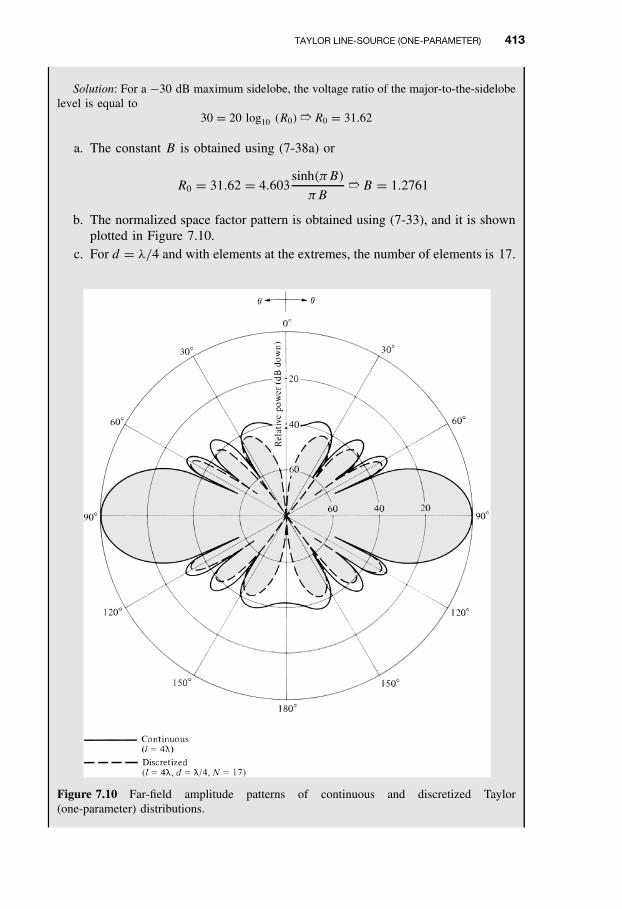
b. The normalized space factor pattern is obtained using (7-33), and it is shownplotted in Figure 7.10.

c. For d = λ/4 and with elements at the extremes, the number of elements is 17.

Figure 7.10 Far-field amplitude patterns of continuous and discretized Taylor(one-parameter) distributions.


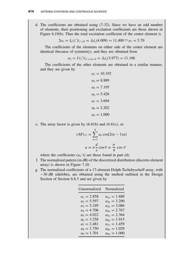
d. The coefficients are obtained using (7-32). Since we have an odd numberof elements, their positioning and excitation coefficients are those shown inFigure 6.19(b). Thus the total excitation coefficient of the center element is

2a1 = In(z′)|z′=0 = J0(j4.009) = 11.400 ➱ a1 = 5.70

The coefficients of the elements on either side of the center element areidentical (because of symmetry), and they are obtained from

a2 = I (z′)|z′=±λ/4 = J0(j3.977) = 11.106

The coefficients of the other elements are obtained in a similar manner,and they are given by

a3 = 10.192

a4 = 8.889

a5 = 7.195

a6 = 5.426

a7 = 3.694

a8 = 2.202

a9 = 1.000

e. The array factor is given by (6-61b) and (6-61c), or

(AF)17 =9∑

n=1

an cos[2(n− 1)u]

u = πd

λcos θ = π

4cos θ

where the coefficients (an’s) are those found in part (d).f. The normalized pattern (in dB) of the discretized distribution (discrete-element

array) is shown in Figure 7.10.g. The normalized coefficients of a 17-element Dolph-Tschebyscheff array, with−30 dB sidelobes, are obtained using the method outlined in the DesignSection of Section 6.8.3 and are given by

Unnormalized Normalized

a1 = 2.858 a1n = 1.680a2 = 5.597 a2n = 3.290a3 = 5.249 a3n = 3.086a4 = 4.706 a4n = 2.767a5 = 4.022 a5n = 2.364a6 = 3.258 a6n = 1.915a7 = 2.481 a7n = 1.459a8 = 1.750 a8n = 1.029a9 = 1.701 a9n = 1.000


As with the discretized Taylor distribution array, the coefficients are symmetrical,and the form of the array factor is that given in part (e).

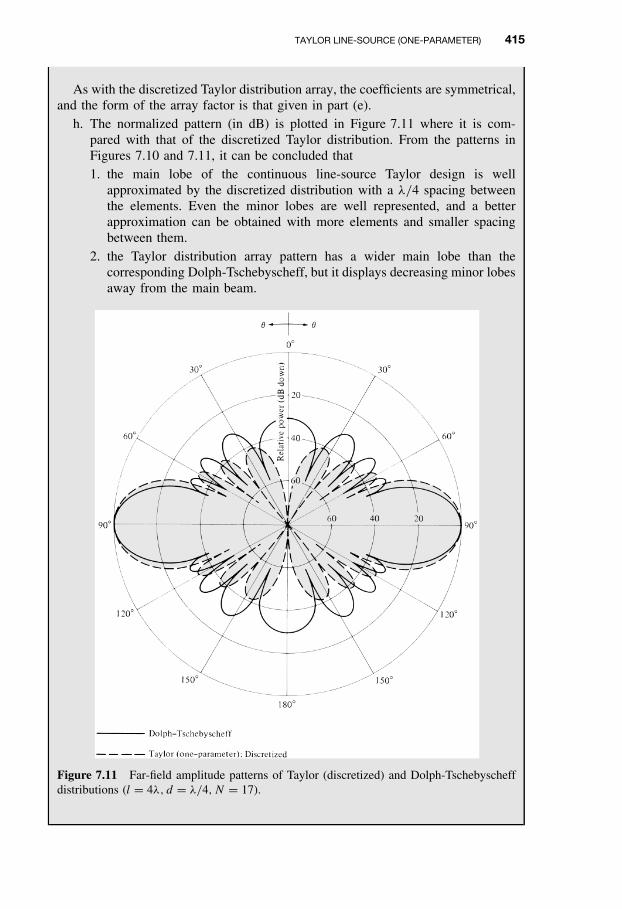
h. The normalized pattern (in dB) is plotted in Figure 7.11 where it is com-pared with that of the discretized Taylor distribution. From the patterns inFigures 7.10 and 7.11, it can be concluded that1. the main lobe of the continuous line-source Taylor design is well

approximated by the discretized distribution with a λ/4 spacing betweenthe elements. Even the minor lobes are well represented, and a betterapproximation can be obtained with more elements and smaller spacingbetween them.

2. the Taylor distribution array pattern has a wider main lobe than thecorresponding Dolph-Tschebyscheff, but it displays decreasing minor lobesaway from the main beam.

Figure 7.11 Far-field amplitude patterns of Taylor (discretized) and Dolph-Tschebyscheffdistributions (l = 4λ, d = λ/4, N = 17).


A larger spacing between the elements does not approximate the continuous distri-bution as accurately. The design of Taylor and Dolph-Tschebyscheff arrays for l = 4λand d = λ/2(N = 9) is assigned as a problem at the end of the chapter (Problem 7.29).

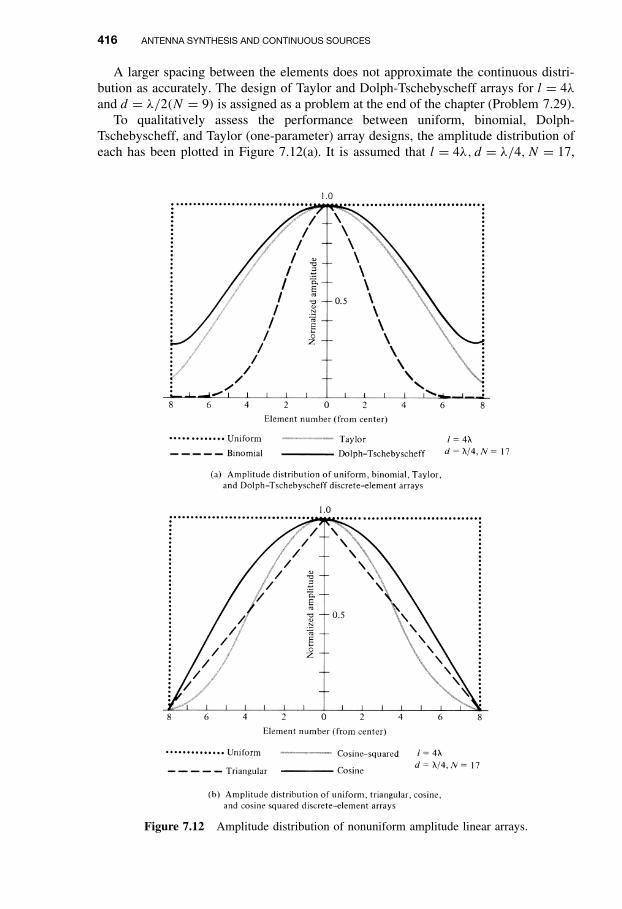
To qualitatively assess the performance between uniform, binomial, Dolph-Tschebyscheff, and Taylor (one-parameter) array designs, the amplitude distribution ofeach has been plotted in Figure 7.12(a). It is assumed that l = 4λ, d = λ/4, N = 17,

Figure 7.12 Amplitude distribution of nonuniform amplitude linear arrays.

TRIANGULAR, COSINE, AND COSINE-SQUARED AMPLITUDE DISTRIBUTIONS 417

and the maximum sidelobe is 30 dB down. The coefficients are normalized with respectto the amplitude of the corresponding element at the center of that array.

The binomial design possesses the smoothest amplitude distribution (between 1and 0) from the center to the edges (the amplitude toward the edges is vanishinglysmall). Because of this characteristic, the binomial array displays the smallest sidelobesfollowed, in order, by the Taylor, Tschebyscheff, and the uniform arrays. In contrast,the uniform array possesses the smallest half-power beamwidth followed, in order,by the Tschebyscheff, Taylor, and binomial arrays. As a rule of thumb, the array withthe smoothest amplitude distribution (from the center to the edges) has the smallestsidelobes and the larger half-power beamwidths. The best design is a trade-off betweensidelobe level and beamwidth.

A MATLAB computer program entitled Synthesis has been developed, and itperforms synthesis using the Schelkunoff, Fourier transform, Woodward-Lawson,Taylor (Tschebyscheff-error) and Taylor (one-parameter) methods. The program isincluded in the CD attached to the book. The description of the program is providedin the corresponding READ ME file.

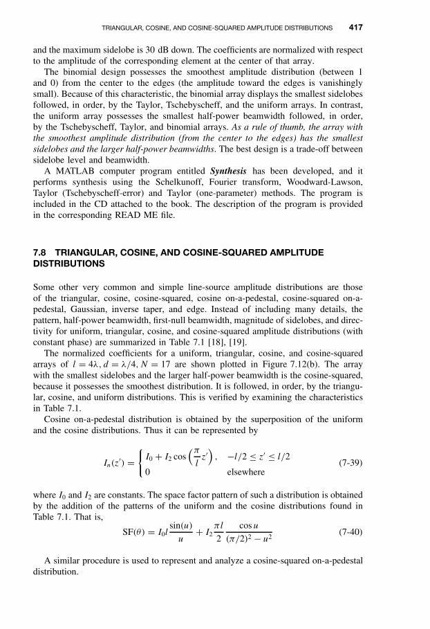
7.8 TRIANGULAR, COSINE, AND COSINE-SQUARED AMPLITUDEDISTRIBUTIONS

Some other very common and simple line-source amplitude distributions are thoseof the triangular, cosine, cosine-squared, cosine on-a-pedestal, cosine-squared on-a-pedestal, Gaussian, inverse taper, and edge. Instead of including many details, thepattern, half-power beamwidth, first-null beamwidth, magnitude of sidelobes, and direc-tivity for uniform, triangular, cosine, and cosine-squared amplitude distributions (withconstant phase) are summarized in Table 7.1 [18], [19].

The normalized coefficients for a uniform, triangular, cosine, and cosine-squaredarrays of l = 4λ, d = λ/4, N = 17 are shown plotted in Figure 7.12(b). The arraywith the smallest sidelobes and the larger half-power beamwidth is the cosine-squared,because it possesses the smoothest distribution. It is followed, in order, by the triangu-lar, cosine, and uniform distributions. This is verified by examining the characteristicsin Table 7.1.

Cosine on-a-pedestal distribution is obtained by the superposition of the uniformand the cosine distributions. Thus it can be represented by

In(z′) =

{I0 + I2 cos

(πlz′), −l/2 ≤ z′ ≤ l/2

0 elsewhere(7-39)

where I0 and I2 are constants. The space factor pattern of such a distribution is obtainedby the addition of the patterns of the uniform and the cosine distributions found inTable 7.1. That is,

SF(θ) = I0lsin(u)

u+ I2

πl

2

cosu

(π/2)2 − u2(7-40)

A similar procedure is used to represent and analyze a cosine-squared on-a-pedestaldistribution.


TABLE 7.1 Radiation Characteristics for Line-Sources and Linear Arrays withUniform, Triangular, Cosine, and Cosine-Squared Distributions

Distribution Uniform Triangular Cosine Cosine-Squared

DistributionIn(analytical)

I0 I1

(1− 2

l|z′|)

I2 cos(πlz′)

I3 cos2(πlz′)

Distribution(graphical)

Space factor(SF) u =(πl

λ

)cos θ

I0lsin(u)

u I1l

2

sin

(u2

)u

2

2

I2lπ

2

cos(u)

(π/2)2 − u2I3l

2

sin(u)

u

[π2

π2 − u2

]

Space factor|SF|

Half-powerbeamwidth(degrees)l � λ

50.6

(l/λ)

73.4

(l/λ)

68.8

(l/λ)

83.2

(l/λ)

First-nullbeamwidth(degrees)l � λ

114.6

(l/λ)

229.2

(l/λ)

171.9

(l/λ)

229.2

(l/λ)

First sidelobemax. (tomain max.)(dB)

−13.2 −26.4 −23.2 −31.5

Directivityfactor(l large)

2

(l

λ

)0.75

[2

(l

λ

)]0.810

[2

(l

λ

)]0.667

[2

(l

λ

)]

7.9 LINE-SOURCE PHASE DISTRIBUTIONS

The amplitude distributions of the previous section were assumed to have uniformphase variations throughout the physical extent of the source. Practical radiators (suchas reflectors, lenses, horns, etc.) have nonuniform phase fronts caused by one or moreof the following:

1. displacement of the reflector feed from the focus2. distortion of the reflector or lens surface

CONTINUOUS APERTURE SOURCES 419

3. feeds whose wave fronts are not ideally cylindrical or spherical (as they areusually presumed to be)

4. physical geometry of the radiator

These are usually referred to phase errors, and they are more evident in radiators withtilted beams.

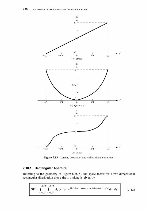
To simplify the analytical formulations, most of the phase fronts are representedwith linear, quadratic, or cubic distributions. Each of the phase distributions can beassociated with each of the amplitude distributions. In (7-1), the phase distribution ofthe source is represented by φn(z

′). For linear, quadratic, and cubic phase variations,φn(z

′) takes the form of

linear: φ1(z′) = β1

2

lz′, −l/2 ≤ z′ ≤ l/2

quadratic: φ2(z′) = β2

(2

l

)2

z′2, −l/2 ≤ z′ ≤ l/2

cubic: φ3(z′) = β3

(2

l

)3

z′3, −l/2 ≤ z′ ≤ l/2

(7-41a)

(7-41b)

(7-41c)

and it is shown plotted in Figure 7.13. The quadratic distribution is used to representthe phase variations at the aperture of a horn and of defocused (along the symmetryaxis) reflector and lens antennas.

The space factor patterns corresponding to the phase distributions of (7-41a)–(7-41c)can be obtained by using (7-1). Because the analytical formulations become lengthy andcomplex, especially for the quadratic and cubic distributions, they will not be includedhere. Instead, a general guideline of their effects will be summarized [18], [19].

Linear phase distributions have a tendency to tilt the main beam of an antennaby an angle θ0 and to form an asymmetrical pattern. The pattern of this distributioncan be obtained by replacing the u (for uniform phase) in Table 7.1 by (u− θ0). Ingeneral, the half-power beamwidth of the tilted pattern is increased by 1/cos θ0 whilethe directivity is decreased by cos θ0. This becomes more apparent by realizing thatthe projected length of the line-source toward the maximum is reduced by cos θ0. Thusthe effective length of the source is reduced.

Quadratic phase errors lead primarily to a reduction of directivity, and an increasein sidelobe level on either side of the main lobe. The symmetry of the original patternis maintained. In addition, for moderate phase variations, ideal nulls in the patternsdisappear. Thus the minor lobes blend into each other and into the main beam, andthey represent shoulders of the main beam instead of appearing as separate lobes.Analytical formulations for quadratic phase distributions are introduced in Chapter 13on horn antennas.

Cubic phase distributions introduce not only a tilt in the beam but also decrease thedirectivity. The newly formed patterns are asymmetrical. The minor lobes on one sideare increased in magnitude and those on the other side are reduced in intensity.

7.10 CONTINUOUS APERTURE SOURCES

Space factors for aperture (two-dimensional) sources can be introduced in a similarmanner as in Section 7.2.1 for line-sources.


Figure 7.13 Linear, quadratic, and cubic phase variations.

7.10.1 Rectangular Aperture

Referring to the geometry of Figure 6.28(b), the space factor for a two-dimensionalrectangular distribution along the x-y plane is given by

SF =∫ ly/2

−ly/2

∫ lx/2

−lx/2An(x

′, y ′)ej [kx ′ sin θ cosφ+ky ′ sin θ sinφ+φn(x ′,y ′)] dx ′ dy ′ (7-42)

CONTINUOUS APERTURE SOURCES 421

where lx and ly are, respectively, the linear dimensions of the rectangular aperturealong the x and y axes. An(x

′, y ′) and φn(x ′, y ′) represent, respectively, the amplitudeand phase distributions on the aperture.

For many practical antennas (such as waveguides, horns, etc.) the aperture distribu-tion (amplitude and phase) is separable. That is,

An(x′, y ′) = Ix(x

′)Iy(y ′) (7-42a)

φn(x′, y ′) = φx(x

′)+ φy(y′) (7-42b)

so that (7-42) can be written asSF = SxSy (7-43)

where

Sx =∫ lx/2

−lx/2Ix(x

′)ej [kx ′ sin θ cosφ+φx(x ′)] dx ′ (7-43a)

Sy =∫ ly/2

−ly/2Iy(y

′)ej [ky ′ sin θ sinφ+φy(y ′)] dy ′ (7-43b)

which is analogous to the array factor of (6-85)–(6-85b) for discrete-element arrays.The evaluation of (7-42) can be accomplished either analytically or graphically. If

the distribution is separable, as in (7-42a) and (7-42b), the evaluation can be performedusing the results of a line-source distribution.

The total field of the aperture antenna is equal to the product of the element andspace factors. As for the line-sources, the element factor for apertures depends on thetype of equivalent current density and its orientation.

7.10.2 Circular Aperture

The space factor for a circular aperture can be obtained in a similar manner as for therectangular distribution. Referring to the geometry of Figure 6.37, the space factor fora circular aperture with radius a can be written as

SF(θ, φ) =∫ 2π

0

∫ a

0An(ρ

′, φ′)ej [kρ ′ sin θ cos(φ−φ′)+ζn(ρ ′,φ′)]ρ ′ dρ ′ dφ′ (7-44)

where ρ ′ is the radial distance (0 ≤ ρ ′ ≤ a), φ′ is the azimuthal angle over the aperture(0 ≤ φ′ ≤ 2π for 0 ≤ ρ ′ ≤ a), and An(ρ

′, φ′) and ζn(ρ ′, φ′) represent, respectively, theamplitude and phase distributions over the aperture. Equation (7-44) is analogous tothe array factor of (6-112a) for discrete elements.

If the aperture distribution has uniform phase [ζn(ρ ′, φ′) = ζ0 = 0] and azimuthalamplitude symmetry [An(ρ

′, φ′) = An(ρ′)], (7-44) reduces, by using (5-48), to

SF(θ) = 2π∫ a

0An(ρ

′)J0(kρ′ sin θ)ρ ′ dρ ′ (7-45)

where J0(x) is the Bessel function of the first kind and of order zero.


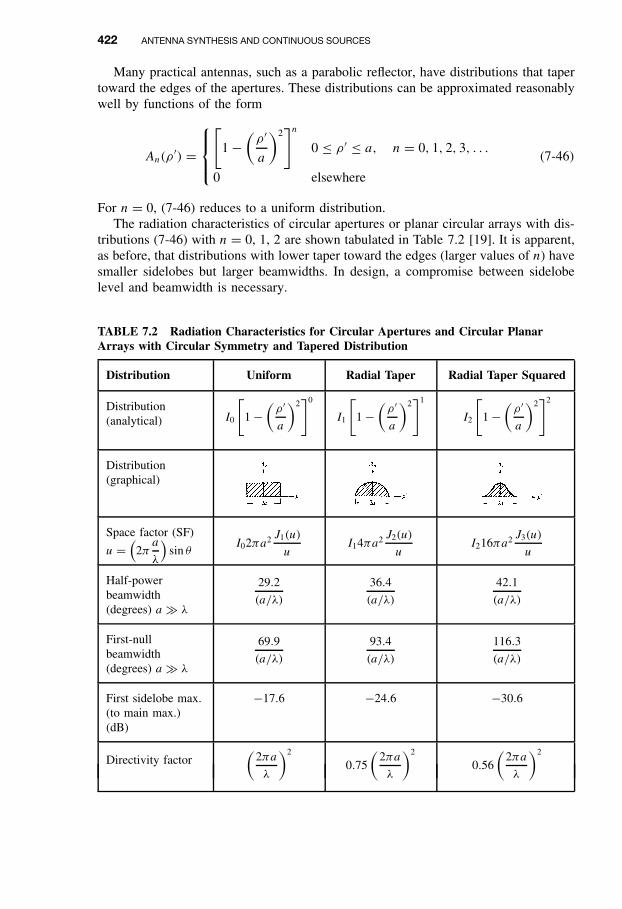
Many practical antennas, such as a parabolic reflector, have distributions that tapertoward the edges of the apertures. These distributions can be approximated reasonablywell by functions of the form

An(ρ′) =

[

1−(ρ ′

a

)2]n

0 ≤ ρ ′ ≤ a, n = 0, 1, 2, 3, . . .

0 elsewhere

(7-46)

For n = 0, (7-46) reduces to a uniform distribution.The radiation characteristics of circular apertures or planar circular arrays with dis-

tributions (7-46) with n = 0, 1, 2 are shown tabulated in Table 7.2 [19]. It is apparent,as before, that distributions with lower taper toward the edges (larger values of n) havesmaller sidelobes but larger beamwidths. In design, a compromise between sidelobelevel and beamwidth is necessary.

TABLE 7.2 Radiation Characteristics for Circular Apertures and Circular PlanarArrays with Circular Symmetry and Tapered Distribution

Distribution Uniform Radial Taper Radial Taper Squared

Distribution(analytical) I0

[1−

(ρ ′

a

)2]0

I1

[1−

(ρ ′

a

)2]1

I2

[1−

(ρ ′

a

)2]2

Distribution(graphical)

Space factor (SF)

u =(

2πa

λ

)sin θ

I02πa2 J1(u)

uI14πa2 J2(u)

uI216πa2 J3(u)

u

Half-powerbeamwidth(degrees) a � λ

29.2

(a/λ)

36.4

(a/λ)

42.1

(a/λ)

First-nullbeamwidth(degrees) a � λ

69.9

(a/λ)

93.4

(a/λ)

116.3

(a/λ)

First sidelobe max.(to main max.)(dB)

−17.6 −24.6 −30.6

Directivity factor(

2πa

λ

)2

0.75

(2πa

λ

)2

0.56

(2πa

λ

)2

REFERENCES 423

7.11 MULTIMEDIA

In the CD that is part of the book, the following multimedia resources are included forthe review, understanding, and visualization of the material of this chapter:

a. Java-based interactive questionnaire, with answers.b. Java-based applet for computing and displaying the synthesis characteristics of

Schelkunoff, Woodward-Lawson and Tschebyscheff-error designs.c. Matlab computer program, designated Synthesis, for computing and displaying

the radiation characteristics ofž Schelkunoffž Fourier transform (line-source and linear array)ž Woodward-Lawson (line-source and linear array)ž Taylor (Tschebyscheff-error and One-parameter) synthesis designs.

d. Power Point (PPT) viewgraphs, in multicolor.

REFERENCES

1. S. A. Schelkunoff, “A Mathematical Theory of Linear Arrays,” Bell System Technical Jour-nal, Vol. 22, pp. 80–107, 1943.

2. H. G. Booker and P. C. Clemmow, “The Concept of an Angular Spectrum of Plane Waves,and Its Relation to That of Polar Diagram and Aperture Distribution,” Proc. IEE (London),Paper No. 922, Radio Section, Vol. 97, pt. III, pp. 11–17, January 1950.

3. P. M. Woodward, “A Method for Calculating the Field over a Plane Aperture Required toProduce a Given Polar Diagram,” J. IEE, Vol. 93, pt. IIIA, pp. 1554–1558, 1946.

4. P. M. Woodward and J. D. Lawson, “The Theoretical Precision with Which an ArbitraryRadiation-Pattern May be Obtained from a Source of a Finite Size,” J. IEE, Vol. 95, pt. III,No. 37, pp. 363–370, September 1948.

5. T. T. Taylor, “Design of Line-Source Antennas for Narrow Beamwidth and Low Sidelobes,”IRE Trans. Antennas Propagat., Vol. AP-3, No. 1, pp. 16–28, January 1955.

6. T. T. Taylor, “One Parameter Family of Line-Sources Producing Modified Sin(πu)/πuPatterns,” Hughes Aircraft Co. Tech. Mem. 324, Culver City, Calif., Contract AF 19(604)-262-F-14, September 4, 1953.

7. R. S. Elliott, “On Discretizing Continuous Aperture Distributions,” IEEE Trans. AntennasPropagat., Vol. AP-25, No. 5, pp. 617–621, September 1977.

8. R. C. Hansen (ed.), Microwave Scanning Antennas, Vol. I, Academic Press, New York,1964, p. 56.

9. J. Ruze, “Physical Limitations on Antennas,” MIT Research Lab., Electronics Tech. Rept.248, October 30, 1952.

10. M. I. Skolnik, Introduction to Radar Systems, McGraw-Hill, New York, 1962, pp. 320–330.

11. R. S. Elliott, “Criticisms of the Woodward-Lawson Method,” IEEE Antennas PropagationSociety Newsletter, Vol. 30, p. 43, June 1988.

12. H. Steyskal, “The Woodward-Lawson Method: A Second Opinion,” IEEE Antennas Prop-agation Society Newsletter, Vol. 30, p. 48, October 1988.


13. R. S. Elliott, “More on the Woodward-Lawson Method,” IEEE Antennas Propagation Soci-ety Newsletter, Vol. 30, pp. 28–29, December 1988.

14. H. Steyskal, “The Woodward-Lawson Method-To Bury or Not to Bury,” IEEE AntennasPropagation Society Newsletter, Vol. 31, pp. 35–36, February 1989.

15. H. J. Orchard, R. S. Elliott, and G. J. Stern. “Optimizing the Synthesis of Shaped BeamAntenna Patterns,” IEE Proceedings, Part H, pp. 63–68, 1985.

16. R. S. Elliott, “Design of Line-Source Antennas for Narrow Beamwidth and AsymmetricLow Sidelobes,” IEEE Trans. Antennas Propagat., Vol. AP-23, No. 1, pp. 100–107, January1975.

17. G. N. Watson, A Treatise on the Theory of Bessel Functions, 2nd. Ed., Cambridge UniversityPress, London, pp. 50 and 379, 1966.

18. S. Silver (ed.), Microwave Antenna Theory and Design, MIT Radiation Laboratory Series,Vol. 12, McGraw-Hill, New York, 1965, Chapter 6, pp. 169–199.

19. R. C. Johnson and H. Jasik (eds.), Antenna Engineering Handbook, 2nd. Ed., McGraw-Hill,New York, 1984, pp. 2–14 to 2-41.

PROBLEMS

7.1. A three-element array is placed along the z-axis. Assuming the spacing betweenthe elements is d = λ/4 and the relative amplitude excitation is equal to a1 =1, a2 = 2, a3 = 1,(a) find the angles where the array factor vanishes when β = 0, π/2, π , and

3π/2(b) plot the relative pattern for each array factorUse Schelkunoff’s method.

7.2. Design a linear array of isotropic elements placed along the z-axis such thatthe zeros of the array factor occur at θ = 0◦, 60◦, and 120◦. Assume that theelements are spaced λ/4 apart and that the progressive phase shift betweenthem is 0◦.(a) Find the required number of elements.(b) Determine their excitation coefficients.(c) Write the array factor.(d) Plot the array factor pattern to verify the validity of the design.Verify using the computer program Synthesis.

7.3. To minimize interference between the operational system, whose antenna isa linear array with elements placed along the z-axis, and other undesiredsources of radiation, it is required that nulls be placed at elevation angles ofθ = 0◦, 60◦, 120◦, and 180◦. The elements will be separated with a uniformspacing of λ/4. Choose a synthesis method that will allow you to design suchan array that will meet the requirements of the amplitude pattern of the arrayfactor. To meet the requirements:(a) Specify the synthesis method you will use.(b) Determine the number of elements.(c) Find the excitation coefficients.

7.4. It is desired to synthesize a discrete array of vertical infinitesimal dipoles placedalong the z-axis with a spacing of d = λ/2 between the adjacent elements. It is

PROBLEMS 425

desired for the array factor to have nulls along θ = 60◦, 90◦, and 120◦. Assumethere is no initial progressive phase excitation between the elements. To achievethis, determine:(a) number of elements.(b) excitation coefficients.(c) angles (in degrees) of all the nulls of the entire array (including of the actual

elements).

7.5. It is desired to synthesize a linear array of elements with spacing d = 3λ/8.It is important that the array factor (AF) exhibits nulls along θ = 0, 90, and180 degrees. Assume there is no initial progressive phase excitation betweenthe elements (i.e., β = 0). To achieve this design, determine:(a) The number of elements(b) The excitation coefficients (amplitude and phase)

If the design allows the progressive phase shift (β) to change, while main-taining the spacing constant (d = 3λ/8),

(c) What would it be the range of possible values for the progressive phase shiftto cause the null at θ = 90 degrees disappear (to place its correspondingroot outside the visible region)?

7.6. The z-plane array factor of an array of isotropic elements placed along thez-axis is given by

AF = z(z4 − 1)

Determine the(a) number of elements of the array. If there are any elements with zero exci-

tation coefficients (null elements), so indicate(b) position of each element (including that of null elements) along the z axis(c) magnitude and phase (in degrees) excitation of each element(d) angles where the pattern vanishes when the total array length (including

null elements) is 2λVerify using the computer program Synthesis.

7.7. Repeat Problem 7.6 whenAF = z(z3 − 1)

7.8. The z-plane array factor of an array of isotropic elements placed along thez-axis is given by (assume β = 0)

AF(z) = (z + 1)3

Determine the(a) Number of elements of the discrete array to have such an array factor.(b) Normalized excitation coefficients of each of the elements of the array (the

ones at the edges to be unity).(c) Classical name of the array design with these excitation coefficients.(d) Angles in theta (θ in degrees) of all the nulls of the array factor when the

spacing d between the elements is d = λ/2.


(e) Half-power beamwidth (in degrees) of the array factor when d = λ/2.(f) Maximum directivity (dimensionless and in dB ) of the array factor when

d = λ/2.

7.9. The z-plane array factor of an array of isotropic elements placed along thez-axis is given by (assume β = 0)

AF(z) = (z + 1)4

Determine the(a) Number of elements of the discrete array to have such an array factor.(b) Normalized excitation coefficients of each of the elements of the array (the

ones at the edges to be unity).(c) Classical name of the array design with these excitation coefficients.(d) Angles in theta (θ in degrees) of all the nulls of the array factor when the

spacing d between the elements is1. d = λ0/42. d = λ0/2

(e) Half-power beamwidth (in degrees) of the array factor when d = λ0/2.(f) Maximum directivity (dimensionless and in dB ) of the array factor when

d = λ0/2.

7.10. The desired array factor in complex form (z-plane) of an array, with the ele-ments along the z-axis, is given by

AF(z) = (z4 −√2z3 + 2z2 −√2z+ 1) = (z2 + 1)(z2 −√2z+ 1)

= (z2 + 1)

[(z2 −√2z+ 1

2

)+ 1

2

]= (z2 + 1)

[(z− 1√

2

)2

+ 1

2

)]where z = x + jy in the complex z-plane.

(a) Determine the number of elements that you will need to realize thisarray factor.

(b) Determine all the roots of this array factor on the unity circle of the com-plex plane.

(c) For a spacing of d = λ/4 and zero initial phase (β = 0), determine all theangles θ (in degrees) where this pattern possesses nulls.

7.11. The z-plane (z = x + jy) array factor of a linear array of elements placed alongthe z-axis, with a uniform spacing d between them and with β = 0, is given by

AF = z(z2 + 1)

Determine, analytically, the(a) number of elements of the array;(b) excitation coefficients;(c) all the roots of the array factor in the visible region only (0 ≤ θ ≤ 180◦)

when d = λ/4;

PROBLEMS 427

(d) all the nulls of the array factor (in degrees) in the visible region only(0 ≤ θ ≤ 180◦) when d = λ/4.

Verify using the computer program Synthesis.

7.12. Repeat Example 7.2 when

SF(θ) ={

1 40◦ ≤ θ ≤ 140◦

0 elsewhere


7.13. Repeat the Fourier transform design of Example 7.2 for a line-source along thez-axis whose sectoral pattern is given by

SF(θ) ={

1 60◦ ≤ θ ≤ 120◦

0 elsewhere

Use l = 5λ and 10λ. Compare the reconstructed patterns with the desired one.Verify using the computer program Synthesis.

7.14. Repeat the Fourier transform design of Problem 7.13 for a linear array with aspacing of d = λ/2 between the elements and(a) N = 11 elements(b) N = 21 elements

7.15. Repeat the design of Problem 7.13 using the Woodward-Lawson method forline sources.

7.16. Repeat the design of Problem 7.14 using the Woodward-Lawson method forlinear arrays for N = 10, 20.

7.17. Design, using the Woodward-Lawson method, a line-source of l = 5λ whosespace factor pattern is given by

SF(θ) = sin3(θ) 0◦ ≤ θ ≤ 180◦

Determine the current distribution and compare the reconstructed pattern withthe desired pattern. Verify using the computer program Synthesis.

7.18. The desired Space Factor SF of a line-source of G = 3λ is the sectoral pattern of

SF =

1

30θ − 2, 60◦ ≤ θ ≤ 90◦

− 1

30θ + 4, 90◦ ≤ θ ≤ 120◦ (θ is in degrees)

0 elsewhere

SF1

q60˚ 90˚ 120˚


It is required to synthesize the desired pattern using the Woodward–Lawsonmethod with odd samples. To accomplish this, determine analytically whenG = 3λ, the(a) number of samples;(b) all the angles (in degrees) where the SF is sampled;(c) all the excitation coefficients bm at the sampling points.Verify using the computer program Synthesis.

7.19. Repeat Problem 7.18 using the Woodward-Lawson method with even samples.

7.20. Repeat the design of Problem 7.17 for a linear array of N = 10 elements witha spacing of d = λ/2 between them.

7.21. In target-search, grounding-mapping radars, and in airport beacons it is desirableto have the echo power received from a target, of constant cross section, to beindependent of its range R.

Generally, the far-zone field radiated by an antenna is given by

|E(R, θ, φ)| = C0|F(θ, φ)|

R

where C0 is a constant. According to the geometry of the figure

R = h/ sin(θ) = h csc (θ)

For a constant value of φ, the radiated field expression reduces to

|E(R, θ, φ = φ0)| = C0|F(θ, φ = φ0)|

R= C1

|f (θ)|R

A constant value of field strength can be maintained provided the radar isflying at a constant altitude h and the far-field antenna pattern is equal to

f (θ) = C2 csc (θ)

This is referred to as a cosecant pattern, and it is used to compensate for therange variations. For very narrow beam antennas, the total pattern is approx-imately equal to the space or array factor. Design a line-source, using theWoodward-Lawson method, whose space factor is given by

SF(θ) ={

0.342 csc (θ), 20◦ ≤ θ ≤ 60◦

0 elsewhere

Plot the synthesized pattern for l = 20λ, and compare it with the desired pattern.Verify using the computer program Synthesis.

7.22. Repeat the design of Problem 7.21 for a linear array of N = 41 elements witha spacing of d = λ/2 between them.

PROBLEMS 429

7.23. For some radar search applications, it is more desirable to have an antennawhich has a square beam for 0 ≤ θ ≤ θ0, a cosecant pattern for θ0 ≤ θ ≤ θm,and it is zero elsewhere. Design a line-source, using the Woodward-Lawsonmethod, with a space factor of

SF(θ) =

1 15◦ ≤ θ < 20◦

0.342 csc (θ) 20◦ ≤ θ ≤ 60◦

0 elsewhere

Plot the reconstructed pattern for l = 20λ, and compare it with thedesired pattern.

7.24. Repeat the design of Problem 7.23, using the Woodward-Lawson method, fora linear array of 41 elements with a spacing of d = λ/2 between them.

7.25. Repeat Problem 7.18 for a linear array of G = 3λ with a spacing of d = 0.5λbetween the elements. Replacing the space factor (SF) of Problem 7.18 with anarray factor (AF) and using the Woodward-Lawson method with odd samples,determine analytically the(a) number of elements;(b) number of samples;(c) angles (in degrees) where the AF is sampled;(d) all the excitation coefficients bm at the sampling points.(e) all the normalized excitation coefficients an of the elements.


7.26. Repeat Problem 7.25 using the Woodward-Lawson method with even samples.

7.27. Design a Taylor (Tschebyscheff-error) line-source with a(a) −25 dB sidelobe level and n = 5(b) −20 dB sidelobe level and n = 10For each, find the half-power beamwidth and plot the normalized current dis-tribution and the reconstructed pattern when l = 10λ. Verify using the com-puter program Synthesis.

7.28. Derive (7-33) using (7-1), (7-32), and Gegenbauer’s finite integral andpolynomials.

7.29. Repeat the design of Example 7.7 for an array with l = 4λ, d = λ/2, N = 9.

7.30. Using a spacing of d = λ/4 between the elements, determine for a Taylor Line-Source (Tschebyscheff-error) of −30 dB, for n = 4 and an equivalent lengthequal to that of 20 discrete elements:(a) The half-power beamwidth (in degrees).(b) State whether the half-power beamwidth in Part a is larger or smaller than

that of an equivalent design for a Dolph-Tschebyscheff array with the samesidelobe level. Explain as to why one is larger or smaller than the other.

(c) The number of complete innermost minor lobes that would have approxi-mately equal sidelobe level.

7.31. Design a broadside five-element, −40 dB sidelobe level Taylor (one-parameter)distribution array of isotropic sources. The elements are placed along the x-axiswith a spacing of λ/4 between them. Determine the


(a) normalized excitation coefficients (amplitude and phase) of each element(b) array factorVerify using the computer program Synthesis.

7.32. Given a continuous line-source, whose total length is 4λ, design a symmetricalTaylor One-Parameter distribution array whose sidelobe is 35 dB down fromthe maximum of the major lobe.(a) Find the constant B.(b) For a spacing of λ between the elements, find the number of discrete ele-

ments needed to approximate the continuous source. Assume that the twoextreme elements are placed at the edges of the continuous line source.

(c) Find the total normalized coefficients (edge elements to be unity) of the dis-crete array of part (c). Identify the position of the corresponding elements.

(d) Write the array factor of the discrete array of parts (c) and (d).Verify using the computer program Synthesis.

7.33. Derive the space factors for uniform, triangular, cosine, and cosine-squaredline-source continuous distributions. Compare with the results in Table 7.1.

7.34. Compute the half-power beamwidth, first-null beamwidth, first sidelobe level(in dB), and directivity of a linear array of closely spaced elements with overalllength of 4λ when its amplitude distribution is(a) uniform (b) triangular(c) cosine (d) cosine-squared

7.35. A nonuniform linear array with a triangular symmetrical distribution consists ofseven discrete elements placed λ/2 apart. The total length (edge-to-edge withelements at the edges) of the array is l = 3λ. Determine the following:(a) Normalized amplitude excitation coefficients (maximum is unity).(b) Half-power beamwidth (in degrees).(c) Maximum directivity (dimensionless and in dB ) for the triangular distribu-

tion.(d) Maximum directivity (dimensionless and in dB ) if the distribution were

uniform. How does it compare with that of Part c? Is it smaller or larger,and by how many dB?

(e) Maximum effective length (assuming that the distribution of the discretearray is the same as that of a continuous line-source) compared to physicallength l:1. If the distribution is triangular.2. If the distribution is uniform.

7.36. Synthesize a 7-element nonuniform array with symmetrical amplitude excitationand with uniform spacing between the elements. The desired amplitude distri-bution across the elements (relative to the center of the array) is cos2 [i.e.,cos2(πx ′/L)] where L is the total length of the array (the end elements are atthe edges of the array length) and x ′ is the position of each element relativeto the center of the array. The overall length L of the array is 3λ. The endelements are at the edges of the array length. Determine the:(a) Spacing between the elements (in λ).

PROBLEMS 431

(b) Normalized total amplitude coefficients of each of the elements (normalizethem so that the amplitude of the center element is unity). Identify each ofthe element position and its corresponding normalized amplitude coefficient.

(c) Approximate half-power beamwidth (in degrees).(d) Approximate maximum directivity (in dB ).

7.37. Derive the space factors for the uniform radial taper, and radial taper-squaredcircular aperture continuous distributions. Compare with the results in Table 7.2.

7.38. Compute the half-power beamwidth, first-null beamwidth, first sidelobe level(in dB), and gain factor of a circular planar array of closely spaced elements,with radius of 2λ when its amplitude distribution is(a) uniform (b) radial taper (c) radial taper-squared.

Documents

CHAPTER7 · antenna pattern synthesis can be classiﬁed into three categories. ... For a continuous source distribution, ... Since physically only sources of ﬁnite dimensions