DIT411/TIN175, Artificial Intelligence Chapters 3–4: More search algorithms

CHAPTERS 3–4: MORE SEARCHCHAPTERS 3–4: MORE SEARCHALGORITHMSALGORITHMS

DIT411/TIN175, Artificial Intelligence

Peter Ljunglöf

23 January, 2018

1

TABLE OF CONTENTSTABLE OF CONTENTSHeuristic search (R&N 3.5–3.6)

Greedy best-first search (3.5.1)A* search (3.5.2)Admissible/consistent heuristics (3.6–3.6.2)

More search strategies (R&N 3.4–3.5)Iterative deepening (3.4.4–3.4.5)Bidirectional search (3.4.6)Memory-bounded A* (3.5.3)

Local search (R&N 4.1)Hill climbing (4.1.1)More local search (4.1.2–4.1.4)Evaluating randomized algorithms

2

HEURISTIC SEARCH (R&N 3.5–3.6)HEURISTIC SEARCH (R&N 3.5–3.6)GREEDY BEST-FIRST SEARCH (3.5.1)GREEDY BEST-FIRST SEARCH (3.5.1)

A* SEARCH (3.5.2)A* SEARCH (3.5.2)

ADMISSIBLE/CONSISTENT HEURISTICS (3.6–3.6.2)ADMISSIBLE/CONSISTENT HEURISTICS (3.6–3.6.2)

3

THE GENERIC TREE SEARCH ALGORITHMTHE GENERIC TREE SEARCH ALGORITHMTree search: Don’t check if nodes are visited multiple times

 function Search(graph, initialState, goalState):

initialise frontier using the initialStatewhile frontier is not empty:

select and remove node from frontierif node.state is a goalState then return nodefor each child in ExpandChildNodes(node, graph):

add child to frontierreturn failure

4

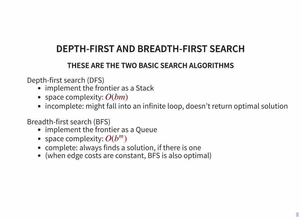
DEPTH-FIRST AND BREADTH-FIRST SEARCHDEPTH-FIRST AND BREADTH-FIRST SEARCHTHESE ARE THE TWO BASIC SEARCH ALGORITHMSTHESE ARE THE TWO BASIC SEARCH ALGORITHMS

Depth-first search (DFS)implement the frontier as a Stackspace complexity: incomplete: might fall into an infinite loop, doesn’t return optimal solution

 Breadth-first search (BFS)

implement the frontier as a Queuespace complexity: complete: always finds a solution, if there is one(when edge costs are constant, BFS is also optimal)

O(bm)

O( )bm

5

COST-BASED SEARCHCOST-BASED SEARCHIMPLEMENT THE FRONTIER AS A PRIORITY QUEUE, ORDERED BY IMPLEMENT THE FRONTIER AS A PRIORITY QUEUE, ORDERED BY

Uniform-cost search (this is not a heuristic algorithm)expand the node with the lowest path cost

= cost from start node to complete and optimal

 Greedy best-first search

expand the node which is closest to the goal (according to some heuristics) = estimated cheapest cost from to a goal

incomplete: might fall into an infinite loop, doesn’t return optimal solution A* search

expand the node which has the lowest estimated cost from start to goal = estimated cost of the cheapest solution through

complete and optimal (if is admissible/consistent)

ff ((nn))

f (n) = g(n) n

f (n) = h(n) n

f (n) = g(n) + h(n) n

h(n)

6

A* TREE SEARCH IS OPTIMAL!A* TREE SEARCH IS OPTIMAL!

A* always finds an optimal solution first, provided that:

the branching factor is finite,

arc costs are bounded above zero (i.e., there is some such that all of the arc costs are greater than ), and

is admissible

i.e., is nonnegative and an underestimate of the cost of the shortest path from to a goal node.

ϵ > 0

ϵ

h(n)

h(n)

n

7

THE GENERIC GRAPH SEARCH ALGORITHMTHE GENERIC GRAPH SEARCH ALGORITHMTree search: Don’t check if nodes are visited multiple timesGraph search: Keep track of visited nodes

 function Search(graph, initialState, goalState):

initialise frontier using the initialStateinitialise exploredSet to the empty setwhile frontier is not empty:

select and remove node from frontierif node.state is a goalState then return nodeadd node to exploredSetfor each child in ExpandChildNodes(node, graph):

add child to frontier if child is not in frontier or exploredSetreturn failure

8

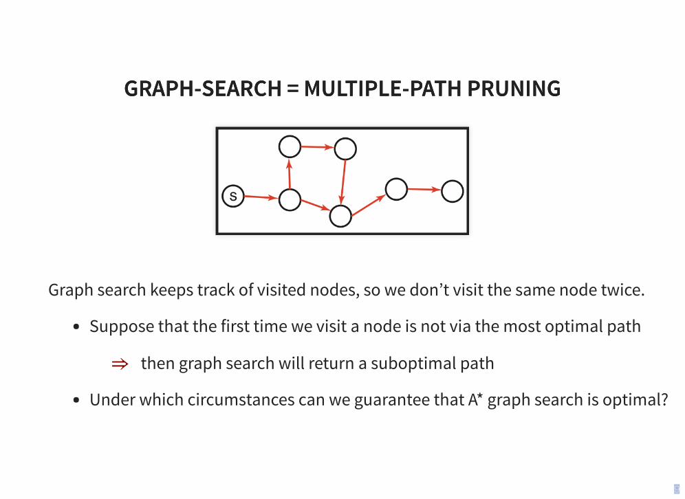
GRAPH-SEARCH = MULTIPLE-PATH PRUNINGGRAPH-SEARCH = MULTIPLE-PATH PRUNING

Graph search keeps track of visited nodes, so we don’t visit the same node twice.

Suppose that the first time we visit a node is not via the most optimal path

        then graph search will return a suboptimal path

Under which circumstances can we guarantee that A* graph search is optimal?

⇒

9

WHEN IS A* GRAPH SEARCH OPTIMAL?WHEN IS A* GRAPH SEARCH OPTIMAL?If   for every arc  , then A* graph search is optimal: 

Lemma: the values along any path are nondecreasing:Proof: , therefore:

therefore: , i.e., is nondecreasing 

Theorem: whenever A* expands a node , the optimal path to has beenfound

Proof: Assume this is not true;then there must be some stillon the frontier, which is on theoptimal path to ;but ;and then must already havebeen expanded contradiction!

|h( ) − h(n)| ≤ cost( , n)n′ n′ ( , n)n′

f [… , , n,…]n′

g(n) = g( ) + cost( , n)n′ n′

f (n) = g(n) + h(n) = g( ) + cost( , n) + h(n) ≥ g( ) + h( )n′ n′ n′ n′

f (n) ≥ f ( )n′ f

n n

n′

n

f ( ) ≤ f (n)n′

n′

⟹

10

CONSISTENCY, OR MONOTONICITYCONSISTENCY, OR MONOTONICITY

A heuristic function is consistent (or monotone) if   for every arc

(This is a form of triangle inequality)

If is consistent, then A* graph search will always finds the shortest path to a goal.

This is a stronger requirement than admissibility.

h

|h(m) − h(n)| ≤ cost(m, n) (m, n)

h

11

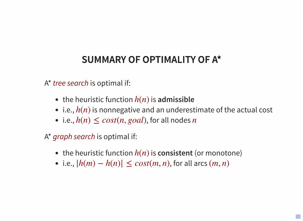
SUMMARY OF OPTIMALITY OF A*SUMMARY OF OPTIMALITY OF A*

A* tree search is optimal if:

the heuristic function is admissiblei.e., is nonnegative and an underestimate of the actual costi.e., , for all nodes

A* graph search is optimal if:

the heuristic function is consistent (or monotone)i.e., , for all arcs

h(n)

h(n)

h(n) ≤ cost(n, goal) n

h(n)

|h(m) − h(n)| ≤ cost(m, n) (m, n)

12

SUMMARY OF TREE SEARCH STRATEGIESSUMMARY OF TREE SEARCH STRATEGIESSearch strategy

Frontier selection

Halts ifsolution?

Halts if nosolution?

Spaceusage

Depth first Last node added No No LinearBreadth first First node added Yes No Exp

Greedy best first Minimal No No Exp

Uniform cost Minimal Optimal No Exp

A* Optimal* No Exp

*Provided that is admissible.

Halts if: If there is a path to a goal, it can find one, even on infinite graphs.Halts if no: Even if there is no solution, it will halt on a finite graph (with cycles).Space: Space complexity as a function of the length of the current path.

h(n)

g(n)

f (n) = g(n) + h(n)

h(n)

13

SUMMARY OF SUMMARY OF GRAPH SEARCHGRAPH SEARCH STRATEGIES STRATEGIESSearch strategy

Frontier selection

Halts ifsolution?

Halts if nosolution?

Spaceusage

Depth first Last node added (Yes)** Yes ExpBreadth first First node added Yes Yes Exp

Greedy best first Minimal No Yes Exp

Uniform cost Minimal Optimal Yes Exp

A* Optimal* Yes Exp

**On finite graphs with cycles, not infinite graphs. *Provided that is consistent.

Halts if: If there is a path to a goal, it can find one, even on infinite graphs.Halts if no: Even if there is no solution, it will halt on a finite graph (with cycles).Space: Space complexity as a function of the length of the current path.

h(n)

g(n)

f (n) = g(n) + h(n)

h(n)

14

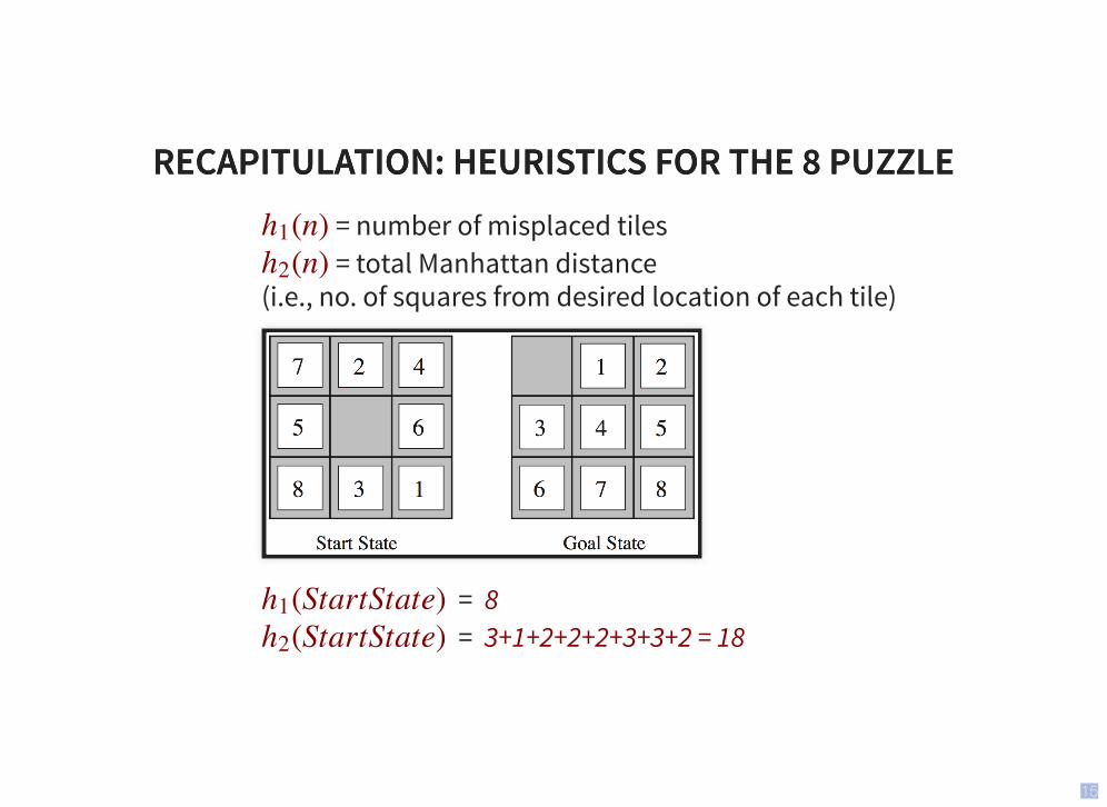
RECAPITULATION: HEURISTICS FOR THE 8 PUZZLERECAPITULATION: HEURISTICS FOR THE 8 PUZZLE = number of misplaced tiles = total Manhattan distance

(i.e., no. of squares from desired location of each tile)

 =  8  =  3+1+2+2+2+3+3+2 = 18

(n)h1

(n)h2

(StartState)h1

(StartState)h2

15

DOMINATING HEURISTICSDOMINATING HEURISTICS

If (admissible) for all , then dominates and is better for search.

Typical search costs (for 8-puzzle):

depth = 14 DFS  ≈  3,000,000 nodes A*( ) = 539 nodes A*( ) = 113 nodes

depth = 24 DFS  ≈  54,000,000,000 nodes A*( ) = 39,135 nodes A*( ) = 1,641 nodes

Given any admissible heuristics , , the maximum heuristics is also admissible and dominates both:

(n) ≥ (n)h2 h1 n

h2 h1

h1

h2

h1

h2

ha hb h(n)

h(n) = max( (n), (n))ha hb

16

HEURISTICS FROM A RELAXED PROBLEMHEURISTICS FROM A RELAXED PROBLEM

Admissible heuristics can be derived from the exact solution cost of a relaxed problem:

If the rules of the 8-puzzle are relaxed so that a tile can move anywhere, then gives the shortest solution

If the rules are relaxed so that a tile can move to any adjacent square, then gives the shortest solution

Key point: the optimal solution cost of a relaxed problem is never greater than the optimal solution cost of the real problem

(n)h1

(n)h2

17

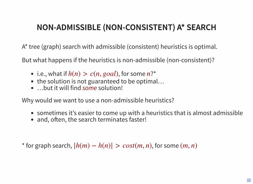
NON-ADMISSIBLE (NON-CONSISTENT) A* SEARCHNON-ADMISSIBLE (NON-CONSISTENT) A* SEARCH

A* tree (graph) search with admissible (consistent) heuristics is optimal.

But what happens if the heuristics is non-admissible (non-consistent)?

i.e., what if , for some ?*the solution is not guaranteed to be optimal……but it will find some solution!

Why would we want to use a non-admissible heuristics?

sometimes it’s easier to come up with a heuristics that is almost admissibleand, o�en, the search terminates faster!

 

* for graph search, , for some

h(n) > c(n, goal) n

|h(m) − h(n)| > cost(m, n) (m, n)

18

EXAMPLE DEMO (AGAIN)EXAMPLE DEMO (AGAIN)Here is an example demo of several different search algorithms, including A*.

Furthermore you can play with different heuristics:

Note that this demo is tailor-made for planar grids, which is a special case of all possible search graphs.

http://qiao.github.io/PathFinding.js/visual/

19

MORE SEARCH STRATEGIES (R&N 3.4–3.5)MORE SEARCH STRATEGIES (R&N 3.4–3.5)ITERATIVE DEEPENING (3.4.4–3.4.5)ITERATIVE DEEPENING (3.4.4–3.4.5)

BIDIRECTIONAL SEARCH (3.4.6)BIDIRECTIONAL SEARCH (3.4.6)

MEMORY-BOUNDED HEURISTIC SEARCH (3.5.3)MEMORY-BOUNDED HEURISTIC SEARCH (3.5.3)

20

ITERATIVE DEEPENINGITERATIVE DEEPENING

BFS is guaranteed to halt but uses exponential space. DFS uses linear space, but is not guaranteed to halt.

Idea: take the best from BFS and DFS — recompute elements of the frontier ratherthan saving them.

Look for paths of depth 0, then 1, then 2, then 3, etc.Depth-bounded DFS can do this in linear space.

Iterative deepening search calls depth-bounded DFS with increasing bounds:

If a path cannot be found at depth-bound, look for a path at depth-bound + 1.Increase depth-bound when the search fails unnaturally (i.e., if depth-bound was reached).

21

ITERATIVE DEEPENING EXAMPLEITERATIVE DEEPENING EXAMPLE

Depth bound = 3

22

ITERATIVE-DEEPENING SEARCHITERATIVE-DEEPENING SEARCH

function IDSearch(graph, initialState, goalState):// returns a solution path, or ‘failure’for limit in 0, 1, 2, …:

result := DepthLimitedSearch([initialState], limit)if result ≠ cutoff then return result

 function DepthLimitedSearch( , limit):

// returns a solution path, or ‘failure’ or ‘cutoff’if is a goalState then return path else if limit = 0 then return cutoffelse:

failureType := failurefor each neighbor of :

result := DepthLimitedSearch( , limit–1)if result is a path then return resultelse if result = cutoff then failureType := cutoff

return failureType

[ ,… , ]n0 nk

nk [ ,… , ]n0 nk

n nk

[ ,… , , n]n0 nk

23

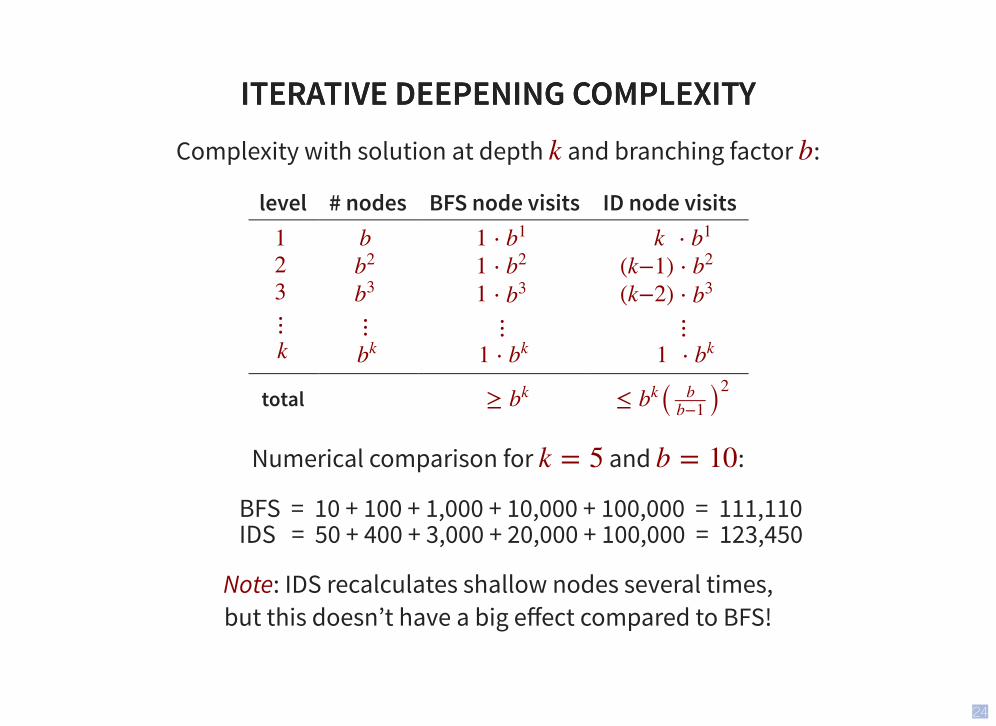
ITERATIVE DEEPENING COMPLEXITYITERATIVE DEEPENING COMPLEXITYComplexity with solution at depth and branching factor :

level # nodes BFS node visits ID node visits

total  

Numerical comparison for and :

BFS  =  10 + 100 + 1,000 + 10,000 + 100,000  =  111,110IDS   =  50 + 400 + 3,000 + 20,000 + 100,000  =  123,450

Note: IDS recalculates shallow nodes several times, but this doesn’t have a big effect compared to BFS!

k b

1

2

3

⋮

k

b

b2

b3

⋮

bk

1 ⋅ b1

1 ⋅ b2

1 ⋅ b3

⋮

1 ⋅ bk

k ⋅ b1

(k−1) ⋅ b2

(k−2) ⋅ b3

⋮

1 ⋅ bk

≥ bk

≤ bk( )b

b−1

2

k = 5 b = 10

24

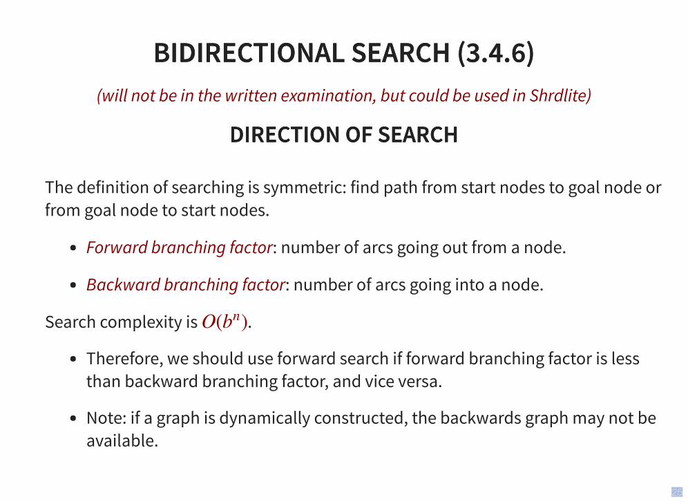
BIDIRECTIONAL SEARCH (3.4.6)BIDIRECTIONAL SEARCH (3.4.6)(will not be in the written examination, but could be used in Shrdlite)

DIRECTION OF SEARCHDIRECTION OF SEARCH

The definition of searching is symmetric: find path from start nodes to goal node orfrom goal node to start nodes.

Forward branching factor: number of arcs going out from a node.

Backward branching factor: number of arcs going into a node.

Search complexity is .

Therefore, we should use forward search if forward branching factor is lessthan backward branching factor, and vice versa.

Note: if a graph is dynamically constructed, the backwards graph may not beavailable.

O( )bn

25

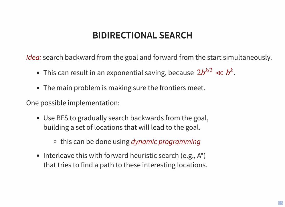
BIDIRECTIONAL SEARCHBIDIRECTIONAL SEARCH

Idea: search backward from the goal and forward from the start simultaneously.

This can result in an exponential saving, because  .

The main problem is making sure the frontiers meet.

One possible implementation:

Use BFS to gradually search backwards from the goal, building a set of locations that will lead to the goal.

this can be done using dynamic programming

Interleave this with forward heuristic search (e.g., A*) that tries to find a path to these interesting locations.

2 ≪bk/2 bk

26

MEMORY-BOUNDED A* (3.5.3)MEMORY-BOUNDED A* (3.5.3)(will not be in the written examination, but could be used in Shrdlite)

A big problem with A* is space usage — is there an iterative deepening version?

IDA*: use the value as the cutoff costthe cutoff is the smalles value that exceeded the previous cutoffo�en useful for problems with unit step costsproblem: with real-valued costs, it risks regenerating too many nodes

RBFS: recursive best-first searchsimilar to DFS, but continues along a path until

is the value of the best alternative path from an ancestorif , recursion unwinds to alternative pathproblem: regenerates too many nodes

SMA* and MA*: (simplified) memory-bounded A*uses all available memorywhen memory is full, it drops the worst leaf node from the frontier

f

f

f (n) > limit

limit f

f (n) > limit

27

LOCAL SEARCH (R&N 4.1)LOCAL SEARCH (R&N 4.1)HILL CLIMBING (4.1.1)HILL CLIMBING (4.1.1)

MORE LOCAL SEARCH (4.1.2–4.1.4)MORE LOCAL SEARCH (4.1.2–4.1.4)

EVALUATING RANDOMIZED ALGORITHMSEVALUATING RANDOMIZED ALGORITHMS

28

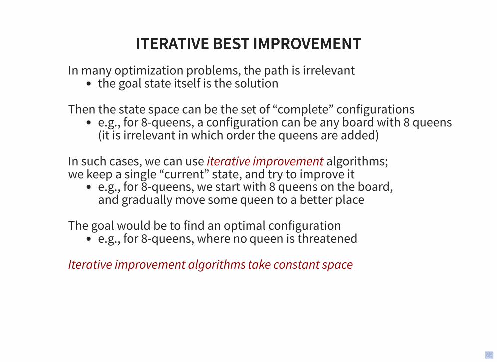
ITERATIVE BEST IMPROVEMENTITERATIVE BEST IMPROVEMENTIn many optimization problems, the path is irrelevant

the goal state itself is the solution Then the state space can be the set of “complete” configurations

e.g., for 8-queens, a configuration can be any board with 8 queens (it is irrelevant in which order the queens are added)

 In such cases, we can use iterative improvement algorithms; we keep a single “current” state, and try to improve it

e.g., for 8-queens, we start with 8 queens on the board, and gradually move some queen to a better place

 The goal would be to find an optimal configuration

e.g., for 8-queens, where no queen is threatened Iterative improvement algorithms take constant space

29

EXAMPLE: EXAMPLE: -QUEENS-QUEENS

Put queens on an board, in separate columns

Move a queen to reduce the number of conflicts; repeat until we cannot move any queen anymore      then we are at a local maximum, hopefully it is global too

This almost always solves -queens problems almost instantaneously for very large (e.g., = 1 million)

nn

n n × n

⇒

n

n n

30

EXAMPLE: 8-QUEENSEXAMPLE: 8-QUEENS

 

Move a queen within its column, choose the minimum n:o of conflicts

the best moves are marked above (conflict value: 12)a�er 5 steps we reach a local minimum (conflict value: 1)

31

EXAMPLE: TRAVELLING SALESPERSONEXAMPLE: TRAVELLING SALESPERSON

Start with any complete tour, and perform pairwise exchanges

Variants of this approach can very quickly get within 1% of optimal solution for thousands of cities

32

HILL CLIMBING SEARCH (4.1.1)HILL CLIMBING SEARCH (4.1.1)Also called (gradient/steepest) (ascent/descent),

or greedy local search

function HillClimbing(graph, initialState):current := initialStateloop:

neighbor := a highest-valued successor of currentif neighbor.value ≤ current.value then return currentcurrent := neighbor

33

PROBLEMS WITH HILL CLIMBINGPROBLEMS WITH HILL CLIMBINGLocal maxima   —   Ridges   —   Plateaux

    

34

RANDOMIZED ALGORITHMSRANDOMIZED ALGORITHMS

Consider two methods to find a maximum value:

Greedy ascent: start from some position, keep moving upwards, and report maximum value found

Pick values at random, and report maximum value found

Which do you expect to work better to find a global maximum?

Can a mix work better?

35

RANDOMIZED HILL CLIMBINGRANDOMIZED HILL CLIMBING

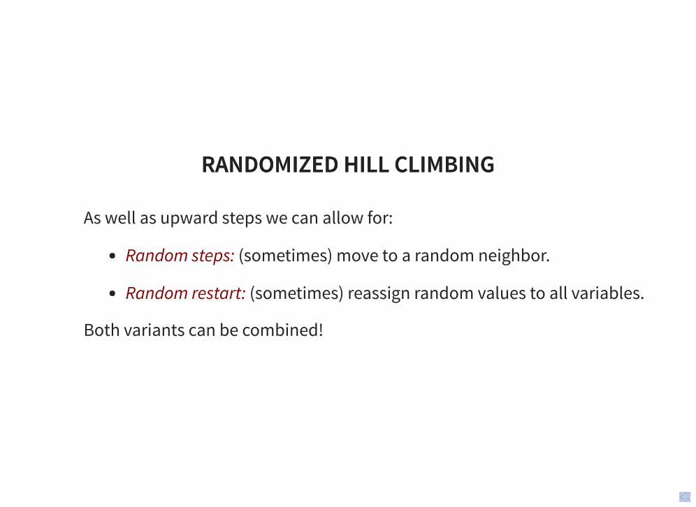
As well as upward steps we can allow for:

Random steps: (sometimes) move to a random neighbor.

Random restart: (sometimes) reassign random values to all variables.

Both variants can be combined!

36

1-DIMENSIONAL ILLUSTRATIVE EXAMPLE1-DIMENSIONAL ILLUSTRATIVE EXAMPLE

Two 1-dimensional search spaces; you can step right or le�:

Which method would most easily find the global maximum?random steps or random restarts?

What if we have hundreds or thousands of dimensions?…where different dimensions have different structure?

37

MORE LOCAL SEARCHMORE LOCAL SEARCH(these sections will not be in the written examination)

SIMULATED ANNEALING (4.1.2)SIMULATED ANNEALING (4.1.2)

BEAM SEARCH (4.1.3)BEAM SEARCH (4.1.3)

GENETIC ALGORITHMS (4.1.4)GENETIC ALGORITHMS (4.1.4)

38

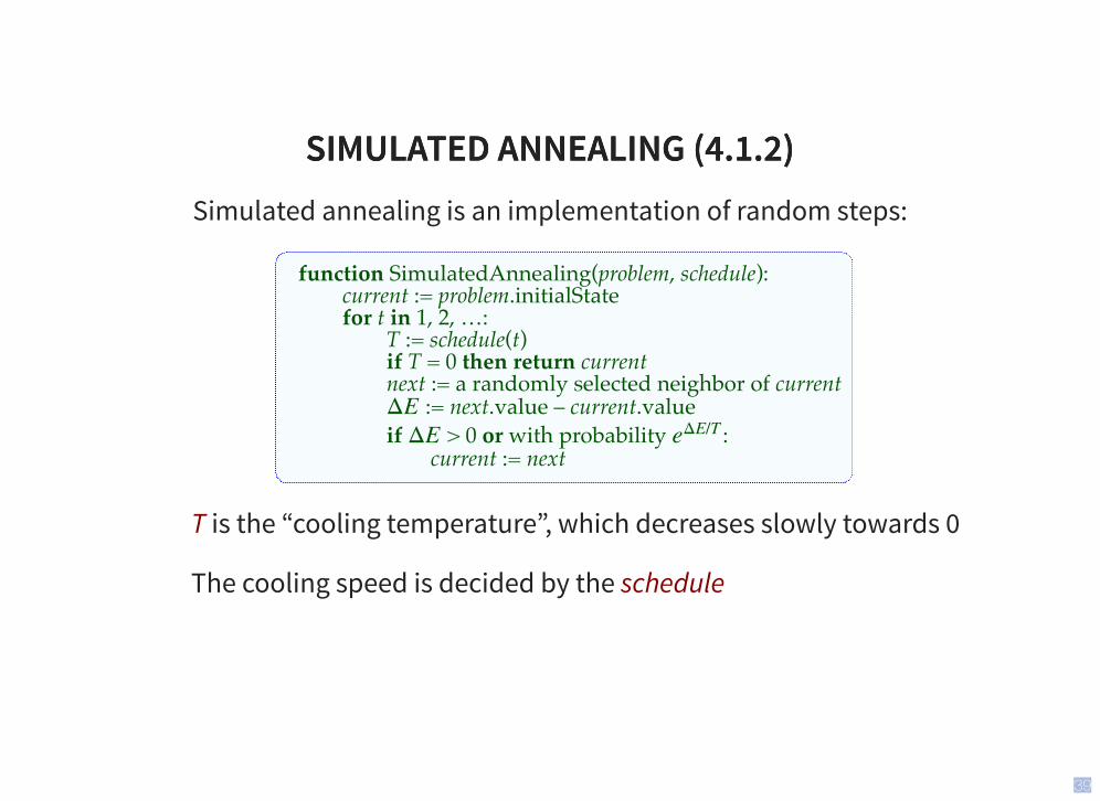
SIMULATED ANNEALING (4.1.2)SIMULATED ANNEALING (4.1.2)Simulated annealing is an implementation of random steps:

function SimulatedAnnealing(problem, schedule):current := problem.initialStatefor t in 1, 2, …:

T := schedule(t)if T = 0 then return currentnext := a randomly selected neighbor of current

:= next.value – current.valueif > 0 or with probability :

current := next

T is the “cooling temperature”, which decreases slowly towards 0

The cooling speed is decided by the schedule

ΔE

ΔE eΔE/T

39

LOCAL BEAM SEARCH (4.1.3)LOCAL BEAM SEARCH (4.1.3)

Idea: maintain a population of states in parallel, instead of one.

At every stage, choose the best out of all of the neighbors.when , it is normal hill climbing searchwhen , it is breadth-first search

The value of lets us limit space and parallelism.

Note: this is not the same as searches run in parallel!

Problem: quite o�en, all states end up on the same local hill.

k

k

k = 1

k = ∞

k

k

k

40

STOCHASTIC BEAM SEARCH (4.1.3)STOCHASTIC BEAM SEARCH (4.1.3)

Similar to beam search, but it chooses the next individuals probabilistically.

The probability that a neighbor is chosen is proportional to its heuristic value.

This maintains diversity amongst the individuals.

The heuristic value reflects the fitness of the individual.

Similar to natural selection: each individual mutates and the fittest ones survive.

k

41

GENETIC ALGORITHMS (4.1.4)GENETIC ALGORITHMS (4.1.4)Similar to stochastic beam search, but pairs of individuals are combined to create the offspring.

For each generation:Randomly choose pairs of individuals where the fittest individuals are more likely to be chosen.For each pair, perform a cross-over: form two offspring each taking different parts of their parents:Mutate some values.

Stop when a solution is found.

42

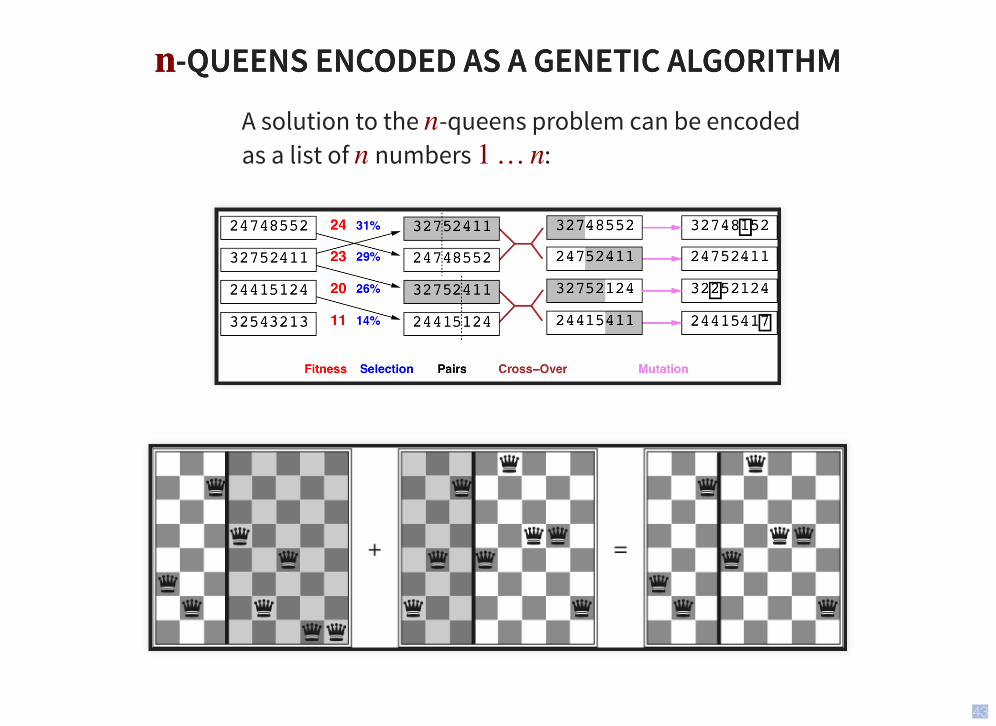
-QUEENS ENCODED AS A GENETIC ALGORITHM-QUEENS ENCODED AS A GENETIC ALGORITHM

A solution to the -queens problem can be encoded as a list of numbers :

nn

n

n 1… n

43

EVALUATING RANDOMIZED ALGORITHMSEVALUATING RANDOMIZED ALGORITHMS(NOT IN R&N)(NOT IN R&N)

(will not be in the written examination)

How can you compare three algorithms A, B and C, when

A solves the problem 30% of the time very quickly but doesn’t halt for the other 70% of the cases

B solves 60% of the cases reasonably quickly but doesn’t solve the rest

C solves the problem in 100% of the cases, but slowly?

Summary statistics, such as mean run time or median run time don’t make much sense.

44

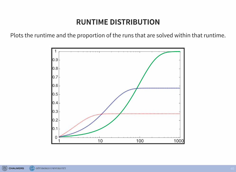
RUNTIME DISTRIBUTIONRUNTIME DISTRIBUTIONPlots the runtime and the proportion of the runs that are solved within that runtime.

45