Embed Size (px)
Citation preview
Lancaster University
Characterisation and PerformanceAnalysis of Random Linear Network
Coding for Reliable and SecureCommunication
Author:
Amjad Saeed Khan
Supervisor:
Dr. Ioannis Chatzigeorgiou
A thesis submitted in partial fulfillment
for the degree of Doctor of Philosophy
Communication Systems Group
School of Computing and Communications
January 25, 2018

Declaration of Authorship
I, Amjad Saeed Khan, declare that this thesis titled, ‘Characterisation and Performance
Analysis of Random Linear Network Coding for Reliable and Secure Communication’
and the work presented in it are my own. I confirm that:
� This work was done wholly or mainly while in candidature for a research degree
at this University.
� Where any part of this thesis has previously been submitted for a degree or any
other qualification at this University or any other institution, this has been clearly
stated.
� Where I have consulted the published work of others, this is always clearly at-
tributed.
� Where I have quoted from the work of others, the source is always given. With
the exception of such quotations, this thesis is entirely my own work.
� I have acknowledged all main sources of help.
� Where the thesis is based on work done by myself jointly with others, I have made
clear exactly what was done by others and what I have contributed myself.
Signed:
Date:
i

Acknowledgements
First of all, I would like to thank Almighty God, the one, who bless me with the oppor-
tunity to pursue the journey towards a PhD.
I would like to express my sincere gratitude and very special thanks to Dr. Ioannis
Chatzigeorgiou for being no less than a perfect supervisor I could ever possibly imagine.
In fact, Ioannis has always impressed me by exceeding all my expectations. He is a real
gentleman and excellent teacher: very supportive, encouraging, understanding, kind,
sincere, honest and generous. Throughout my PhD, Ioannis was not only supporting me
to improve my knowledge and writing expertise, but also seemed to have always a better
thought and plan for my exposure and future development. Apart from the research,
he has given me great advices from his life experience that added a lot of positivity in
my personality, which is priceless to me. I will always be very grateful to Ioannis for
making my graduate experience very productive, enjoyable and memorable.
I wish to thank the Lancaster University for their excellent resources. In particular,
thanks to the School of Computing and Communications (InfoLab21) for providing
the research environment and resources, and for their friendly and supporting faculty
and staff members including: Prof. Zhiguo Ding, Prof. Qiang Ni, Vicky Waddington,
Gillian Balderstone and Debbie Stubbs. Moreover, I am very grateful and thankful
to the Faculty of Science and Technology (FST) for granting me a very precious PhD
scholarship, and providing me support to attend the number of summer schools. The op-
portunity of studying in the Lancaster University will always be a remarkable experience
in my life.
I specially thanks to my father and mother for their never-ending love, prayers, encour-
agements, support and showing confidence on me, without which it would be impossible
for me to pursue my studies up to this stage. In addition, thanks to my sisters and
brother for their love, prayers and encouragements throughout my studies. Further-
more, I wish to thank all my colleagues and sincere friends for helping me with their
valuable discussions and guidance during my PhD. Last but not least, I would like to
thank Andrew Wood and Elspeth Wood, the organizers of Friends International Lan-
caster, for beautifying my stay here at Lancaster, and for being a part of wonderful
memories.
ii
List of Publications
Most of the work documented in this thesis has been published or under preparation for
publication in journals or conference proceedings, as listed below:
Journal
1. A. S. Khan and I. Chatzigeorgiou, “Non-Orthogonal Multiple Access Combined
With Random Linear Network Coded Cooperation”, IEEE Signal Processing Let-
ters, vol. 24, no. 9, pp. 1298-1302, Sept. 2017.
2. A. S. Khan and I. Chatzigeorgiou, “Improved bounds on the decoding failure
probability of linear NC over multi-source multi-relay networks”, IEEE Commu-
nications Letters, vol. 20, no. 10, pp. 2035-2038, Oct. 2016.
3. A. S. Khan, A. Tassi and I. Chatzigeorgiou, “Rethinking the intercept probability
of random linear network coding”, IEEE Communications Letters, vol. 19, no. 10,
pp. 1762-1765, October 2015.
4. A. S. Khan and I. Chatzigeorgiou, “Opportunistic relaying and random linear
network coding for secure and reliable communication”, IEEE Transactions on
Wireless Communications, (accepted with minor revisions).
5. A. S. Khan and I. Chatzigeorgiou, “A Framework for the Analysis of Network-
Coded Schemes Characterized by Random Block Matrices”, IEEE Transactions
on Wireless Communications, (in preparation).
Conference
1. A. S. Khan and I. Chatzigeorgiou, “Performance analysis of random linear net-
work coding in two-source single-relay networks”, in Proc. IEEE International
Conference on Communications Workshops (ICC), Workshop on Cooperative and
Cognitive Networks, London, United Kingdom, June 2015.
iii
LANCASTER UNIVERSITY
Abstract
Faculty of Science and Technology
School of Computing and Communications
Doctor of Philosophy
Characterisation and Performance Analysis of Random Linear Network
Coding for Reliable and Secure Communication
by Amjad Saeed Khan
v
In this thesis, we develop theoretical frameworks to characterize the performance of
Random Linear Network Coding (RLNC), and propose novel communication schemes
for the achievement of both reliability and security in wireless networks. In particular, (i)
we present an analytical model to evaluate the performance of practical RLNC schemes
suitable for low-complexity receivers, prioritized (i.e., layered) coding and multi-hop
communications, (ii) investigate the performance of RLNC in relay assisted networks and
propose a new cross-layer RLNC-aided cooperative scheme for reliable communication,
(iii) characterize the secrecy feature of RLNC and propose a new physical-application
layer security technique for the purpose of achieving security and reliability in multi-hope
communications.
At first, we investigate random block matrices and derive mathematical expressions for
the enumeration of full-rank matrices that contain blocks of random entries arranged
in a diagonal, lower-triangular or tri-diagonal structure. The derived expressions are
then used to model the probability that a receiver will successfully decode a source
message or layers of a service, when RLNC based on non-overlapping, expanding or
sliding generations is employed. Moreover, the design parameters of these schemes allow
to adjust the desired decoding performance.
Next, we evaluate the performance of Random Linear Network Coded Cooperation (RL-
NCC) in relay assisted networks, and propose a cross-layer cooperative scheme which
combines the emerging Non-Orthogonal Multiple Access (NOMA) technique and RL-
NCC. In this regard, we first consider the multiple-access relay channel in a setting
where two source nodes transmit packets to a destination node, both directly and via
a relay node. Secondly, we consider a multi-source multi-relay network, in which relay
nodes employ RLNC on source packets and generate coded packets. For each network,
we build our analysis on fundamental probability expressions for random matrices over
finite fields and we derive theoretical expressions of the probability that the destination
node will successfully decode the source packets. Finally, we consider a multi-relay net-
work comprising of two groups of source nodes, where each group transmits packets to its
own designated destination node over single-hop links and via a cluster of relay nodes
shared by both groups. In an effort to boost reliability without sacrificing through-
put, a scheme is proposed whereby packets at the relay nodes are combined using two
methods; packets delivered by different groups are mixed using non-orthogonal multiple
access principles, while packets originating from the same group are mixed using RLNC.
An analytical framework that characterizes the performance of the proposed scheme is
developed, and benchmarked against a counterpart scheme that is based on orthogonal
multiple access.
vi
Finally, we quantify and characterize the intrinsic security feature of RLNC and design
a joint physical-application layer security technique. For this purpose, we first consider
a network comprising a transmitter, which employs RLNC to encode a message, a le-
gitimate receiver, and a passive eavesdropper. Closed-form analytical expressions are
derived to evaluate the intercept probability of RLNC, and a resource allocation model
is presented to further minimize the intercept probability. Afterward, we propose a joint
RLNC and opportunistic relaying scheme in a multi relay network to transmit confi-
dential data to a destination in the presence of an eavesdropper. Four relay selection
protocols are studied covering a range of network capabilities, such as the availability of
the eavesdropper’s channel state information or the possibility to pair the selected relay
with a jammer node that intentionally generates interference. For each case, expressions
of the probability that a coded packet will not be decoded by a receiver, which can be
either the destination or the eavesdropper, are derived. Based on those expressions, a
framework is developed that characterizes the probability of the eavesdropper intercept-
ing a sufficient number of coded packets and partially or fully decoding the confidential
data. We observe that the field size over which RLNC is performed at the application
layer as well as the adopted modulation and coding scheme at the physical layer can be
modified to fine-tune the trade-off between security and reliability.
Contents
Declaration of Authorship i
Acknowledgements ii
List of Publications iii
Abstract iv
Contents vii
List of Figures x
Abbreviations xiii
1 Introduction 1
1.1 Background and Motivations . . . . . . . . . . . . . . . . . . . . . . . . . 1
1.2 Basic Examples of Network Coding . . . . . . . . . . . . . . . . . . . . . . 2
1.2.1 NC in a Butterfly Network . . . . . . . . . . . . . . . . . . . . . . 3
1.2.2 NC in a Wireless Network . . . . . . . . . . . . . . . . . . . . . . . 4
1.3 Random Linear Network Coding . . . . . . . . . . . . . . . . . . . . . . . 4
1.3.1 RLNC Encoding and Decoding . . . . . . . . . . . . . . . . . . . . 5
1.3.2 RLNC Example . . . . . . . . . . . . . . . . . . . . . . . . . . . . . 6
1.3.3 RLNC Limitation and Literature Work . . . . . . . . . . . . . . . 7
1.4 RLNC Applications . . . . . . . . . . . . . . . . . . . . . . . . . . . . . . 8
1.4.1 RLNC for Heterogeneous Devices and Broadcast Communication . 9
1.4.2 Random Linear Network Coded Cooperation . . . . . . . . . . . . 9
1.4.3 RLNC for Secure Communication . . . . . . . . . . . . . . . . . . 9
1.4.4 RLNC Integrated with Opportunistic Relaying and IntentionalJamming . . . . . . . . . . . . . . . . . . . . . . . . . . . . . . . . 10
1.5 Overview and Contributions of Thesis . . . . . . . . . . . . . . . . . . . . 12
1.5.1 Thesis Structure and Organization . . . . . . . . . . . . . . . . . . 13
2 A Framework for the Assessment of Network Coding Techniques Char-acterized by Random Block Matrices 16
2.1 Fundamental Preliminary Expressions . . . . . . . . . . . . . . . . . . . . 17
vii
Contents viii
2.2 Partitioning of Random Matrices . . . . . . . . . . . . . . . . . . . . . . . 18
2.3 Structures of Random Block Matrices . . . . . . . . . . . . . . . . . . . . 20
2.3.1 Block Diagonal (BD) Matrices . . . . . . . . . . . . . . . . . . . . 21
2.3.2 Block Lower-Triangular (BLT) Matrices . . . . . . . . . . . . . . . 22
2.3.3 Block Tri-Diagonal (BTD) Matrices . . . . . . . . . . . . . . . . . 23
2.4 Assessment of Network Coding Techniques . . . . . . . . . . . . . . . . . . 26
2.4.1 Non-Overlapping Generations RLNC (NOG-RLNC) . . . . . . . . 27
2.4.2 Expanding Generations RLNC (EG-RLNC) . . . . . . . . . . . . . 28
2.4.3 Sliding Generations RLNC (SG-RLNC) . . . . . . . . . . . . . . . 30
2.5 Results and Discussions . . . . . . . . . . . . . . . . . . . . . . . . . . . . 31
2.5.1 Performance Comparison between NOG-RLNC, SG-RLNC andEG-RLNC over Non-erasure Channels . . . . . . . . . . . . . . . . 32
2.5.2 Performance Comparison between SG-RLNC and EG-RLNC overErasure Channels . . . . . . . . . . . . . . . . . . . . . . . . . . . . 35
2.6 Summary . . . . . . . . . . . . . . . . . . . . . . . . . . . . . . . . . . . . 36
3 Random Linear Network Coding for Coded Cooperation 38
3.1 Random Linear Network Coded Cooperation in Two Source Single RelayNetworks . . . . . . . . . . . . . . . . . . . . . . . . . . . . . . . . . . . . 39
3.1.1 System Model and Problem Statement . . . . . . . . . . . . . . . . 39
3.1.2 Performance Analysis . . . . . . . . . . . . . . . . . . . . . . . . . 42
3.1.2.1 Preliminaries: fundamental probability expressions . . . . 42
3.1.2.2 Decoding probability for non-systematic network coding . 43
3.1.2.3 Decoding probability for systematic network coding . . . 45
3.1.3 Results and Discussions . . . . . . . . . . . . . . . . . . . . . . . . 47
3.2 Random Linear Network Coded Cooperation in Multi-source Multi-relayNetworks . . . . . . . . . . . . . . . . . . . . . . . . . . . . . . . . . . . . 49
3.2.1 System Model . . . . . . . . . . . . . . . . . . . . . . . . . . . . . . 49
3.2.2 Preliminary Results and Former Bounds on the Probability of De-coding Failure . . . . . . . . . . . . . . . . . . . . . . . . . . . . . . 50
3.2.3 Improved Bounds on the Probability of Decoding Failure . . . . . 52
3.2.3.1 Upper bound . . . . . . . . . . . . . . . . . . . . . . . . . 52
3.2.3.2 Lower bound . . . . . . . . . . . . . . . . . . . . . . . . . 54
3.2.4 Results and Discussions . . . . . . . . . . . . . . . . . . . . . . . . 54
3.3 Random Linear Network Coded Cooperation Combined with Non-OrthogonalMultiple Access . . . . . . . . . . . . . . . . . . . . . . . . . . . . . . . . . 57
3.3.1 System Model . . . . . . . . . . . . . . . . . . . . . . . . . . . . . . 57
3.3.2 Achievable Rate and Link Outage Probability . . . . . . . . . . . . 59
3.3.3 Decoding Probability and Analysis . . . . . . . . . . . . . . . . . . 61
3.3.4 Results and Discussions . . . . . . . . . . . . . . . . . . . . . . . . 63
3.4 Summary . . . . . . . . . . . . . . . . . . . . . . . . . . . . . . . . . . . . 65
4 Random Linear Network Coding for Secure Communication 67
4.1 The Intercept Probability of RLNC . . . . . . . . . . . . . . . . . . . . . . 68
4.1.1 System Model . . . . . . . . . . . . . . . . . . . . . . . . . . . . . . 69
4.1.2 Performance Analysis . . . . . . . . . . . . . . . . . . . . . . . . . 69
4.1.3 Optimization Model . . . . . . . . . . . . . . . . . . . . . . . . . . 72
4.1.4 Results and Discussions . . . . . . . . . . . . . . . . . . . . . . . . 73
Contents ix
4.2 Opportunistic Relaying and RLNC for Secure and Reliable Communication 75
4.2.1 System Model . . . . . . . . . . . . . . . . . . . . . . . . . . . . . . 75
4.2.2 Relay Selection and Outage Analysis . . . . . . . . . . . . . . . . . 78
4.2.2.1 Relay selection protocols without jammer . . . . . . . . . 79
4.2.2.2 Relay selection protocols with jammer . . . . . . . . . . . 82
4.2.3 Secrecy Analysis . . . . . . . . . . . . . . . . . . . . . . . . . . . . 87
4.2.3.1 Preliminaries . . . . . . . . . . . . . . . . . . . . . . . . . 87
4.2.3.2 Derivation of the τ -intercept probability . . . . . . . . . . 88
4.2.4 Results and Discussions . . . . . . . . . . . . . . . . . . . . . . . . 90
4.3 Summary . . . . . . . . . . . . . . . . . . . . . . . . . . . . . . . . . . . . 96
5 Conclusions and Future Research Directions 97
5.1 Summary and Conclusions of the Thesis . . . . . . . . . . . . . . . . . . . 97
5.2 Future Directions . . . . . . . . . . . . . . . . . . . . . . . . . . . . . . . . 98
A Analytical proof of Lemma 2.1 100
B Reformulation of the intercept probability of FT 101
C Proof of Proposition 4.2 for the case of FT 102
Bibliography 103
List of Figures
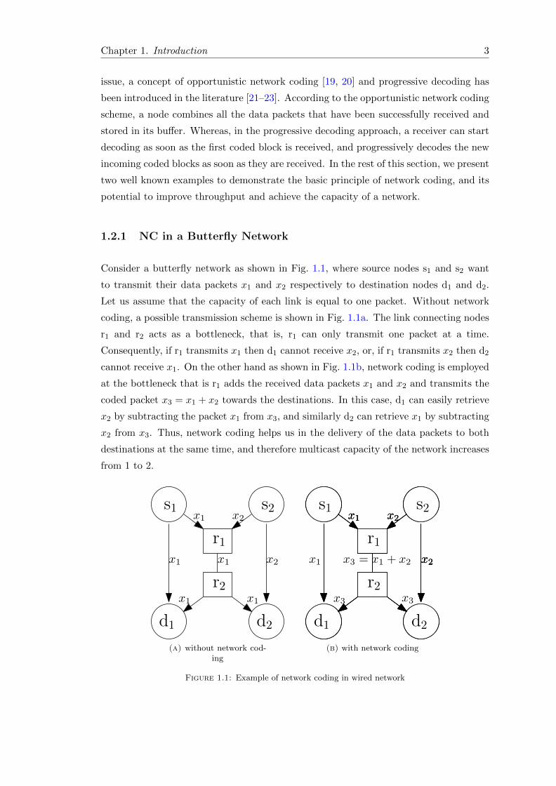
1.1 Example of network coding in wired network . . . . . . . . . . . . . . . . 3
1.2 Example of network coding in wireless network . . . . . . . . . . . . . . . 4
1.3 Structure of transmitted coded packet . . . . . . . . . . . . . . . . . . . . 6
1.4 Example of RLNC in multi-path network . . . . . . . . . . . . . . . . . . 6
1.5 Applications of RLNC . . . . . . . . . . . . . . . . . . . . . . . . . . . . . 8
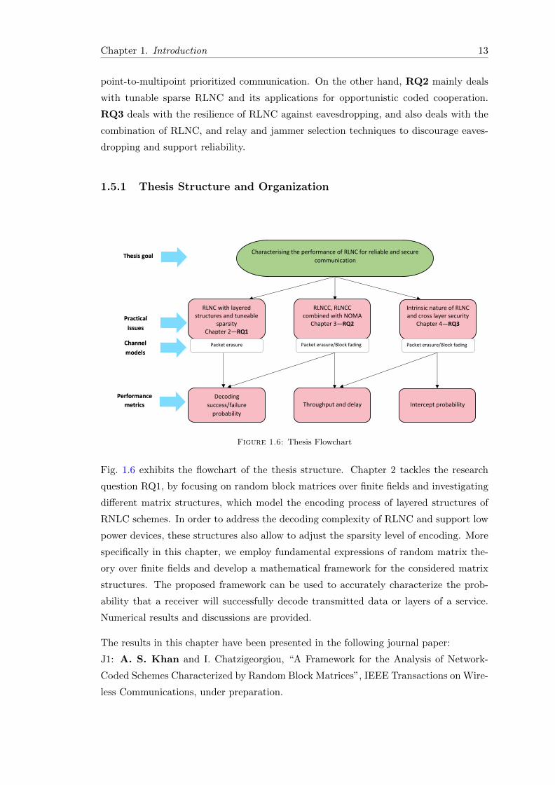
1.6 Thesis Flowchart . . . . . . . . . . . . . . . . . . . . . . . . . . . . . . . . 13
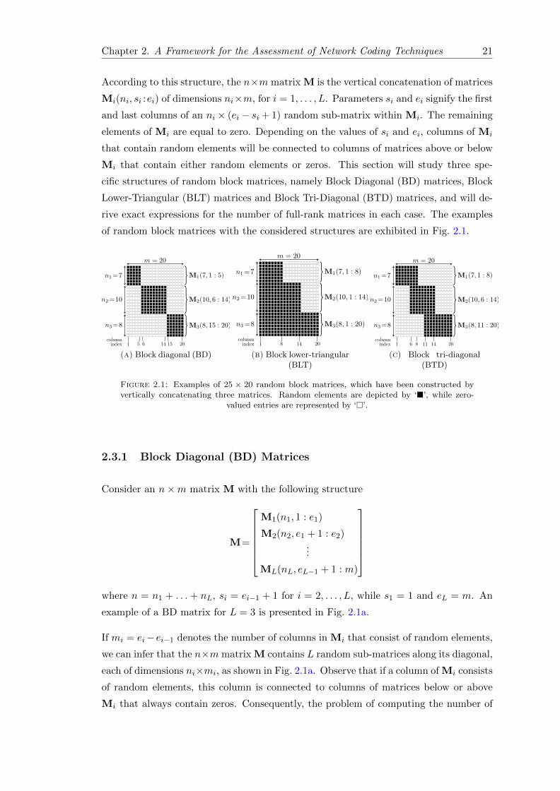
2.1 Examples of 25×20 random block matrices, which have been constructedby vertically concatenating three matrices. Random elements are depictedby ‘�’, while zero-valued entries are represented by ‘�’. . . . . . . . . . . 21
2.2 Example of NOG-RLNC. The source packets x1, . . . , xm have been orga-nized into L generations G1, . . . ,GL. Generation Gi contains ki sourcepackets. . . . . . . . . . . . . . . . . . . . . . . . . . . . . . . . . . . . . . 28
2.3 Example of EG-RLNC. Each generation Gi is nested in generation Gi+1.The number of source packets that belong to a generation Gi but not tolower-indexed generations is denoted by mi. . . . . . . . . . . . . . . . . . 29
2.4 Example of SG-RLNC. Them source packets are members of L contiguousgenerations G1, . . . ,GL. For i > 1, generations Gi−1 and Gi have wi−1
source packets in common. . . . . . . . . . . . . . . . . . . . . . . . . . . . 30
2.5 Comparison between theoretical results for SG-RLNC obtained from (2.25)and simulation results for L = 2 generations and different values of n2.The remaining parameters have been set as follows: q = 2, m = 20,m1 =m2 =10, n1 = n1 =10, n2 = n2 and ε = 0. . . . . . . . . . . . . . . . . 32
2.6 Comparison between NOG-RLNC, SG-RLNC and EG-RLNC for L = 3,m = 60, m1 = m2 = m3 = 20, n1 = n2 = 20 and n3 = 20 + δ3. Variouspercentages of overlap in the case of SG-RLNC have been considered.Furthermore, ni = ni for all values of i, q = 2 and ε = 0. . . . . . . . . . 33
2.7 Comparison between NOG-RLNC, SG-RLNC and EG-RLNC for L = 3,m= 60, m1 =m2 =m3 = 20, n1 = n2 = n3 = 20 + κ, where κ representsoverhead per generation. In addition, q = 2, ε = 0 and the overlap inSG-RLNC is set to 9% . . . . . . . . . . . . . . . . . . . . . . . . . . . . . 33
2.8 Theoretical predictions and simulation results for SG-RLNC and EG-RLNC, when the field size q is 2, 3, 5 or 7. The system parameters areL = 3, m = 60, m1 =m2 = m3 =20, n1 = n1 =20, n2 = n2 =20 and ε = 0.The overlap in SG-RLNC is fixed at 9%. . . . . . . . . . . . . . . . . . . . 34
2.9 Effect of the field size q on the decoding probability of SG-RLNC andEG-RLNC for L = 3, m= 60, m1 =m2 = m3 = 20 and ε = 0.2. If theoverhead per generation is κ = 0, 1, . . . , 15, the overall overhead is δ = 3κ,i.e., δ = 0, 3, . . . , 45. . . . . . . . . . . . . . . . . . . . . . . . . . . . . . . 34
x
List of Figures xi
2.10 Performance comparison between SG-RLNC and EG-RLNC for m= 60,m1 = m2 = m3 = 20, n1 = n2 = 26, ε ∈ {0.1, 0.2, 0.3, 0.4} and q = 256.Various percentages of overlap for SG-RLNC have been considered. . . . . 35
3.1 Block diagram of a network consisting of two source nodes S1 and S2, arelay node R and a destination node D. The packet erasure probability ofeach link as well as the number of transmitted and received coded packetsat each node are also depicted. . . . . . . . . . . . . . . . . . . . . . . . . 41
3.2 Comparison between theoretical upper bounds obtained from (3.12) andsimulation results for different values of m and n. The erasure probabili-ties have been set to εSD = 0.3, εSR = 0.1 and εRD = 0.2. . . . . . . . . . . 47
3.3 Comparison between theoretical upper bounds obtained from (3.12) andsimulation results for different values of εSD. The remaining system pa-rameters have been set to m = 20, n = 30, εSR = 0.1 and εRD = 0.2. . . . 47
3.4 Performance comparison of systematic and non-systematic network cod-ing as a function of the excess coded packets n−m transmitted by eachsource node for various values of εSR. The remaining system parametershave been set to m = 20, nR = 15, εSD = 0.3 and εRD = 0.1. . . . . . . . . 48
3.5 A network consisting of m source nodes, n ≥ m relay nodes and a desti-nation D. The packet erasure probability of a source-to-relay link and arelay-to-destination link is represented by εSR and εRD, respectively. . . . 50
3.6 Comparison between simulation results and the theoretical upper boundsobtained from (3.24) and (3.28) for different values of m and n, whenq = 2, εRD = 0.1 and εSR ∈ [0.1, 0.9]. . . . . . . . . . . . . . . . . . . . . . 55
3.7 Effect of field size q on network performance and comparison between theproposed bounds and the old bounds for εSR ∈ [0.1, 0.9], when m = 20,n = 25 and εRD = 0.1. . . . . . . . . . . . . . . . . . . . . . . . . . . . . . 55
3.8 Performance of the network for an increasing number of relays n. Theproposed bounds and the old bounds have been plotted for m = 10,εSR = 0.7, εRD = 0.2 and different values of field size q. . . . . . . . . . . . 56
3.9 Network performance and comparison between the proposed bounds andthe old bounds for m = 10, an increasing number of relays n, εSR = 0.3,εRD = 0.1 and different field size q. . . . . . . . . . . . . . . . . . . . . . . 56
3.10 Block diagram of the system model . . . . . . . . . . . . . . . . . . . . . . 58
3.11 Simulation results and performance comparison between NOMA-RLNCand OMA-RLNC, when m = 20, n = 10 and q = 4. . . . . . . . . . . . . . 63
3.12 Effect of the field size q and the number of relay nodes n on the jointdecoding probability, when m = 20. . . . . . . . . . . . . . . . . . . . . . . 64
3.13 Comparison between the two schemes in terms of the required averagenumber of relay nodes and the SNR when m = 20 and q = 4. . . . . . . . 65
3.14 Effect of target rates on the system throughput against the system SNR,when m = 20 and q = 4. . . . . . . . . . . . . . . . . . . . . . . . . . . . . 65
4.1 Block diagram of the system model, where εB and εE denote the era-sure probabilities of the channels linking Alice to Bob and Alice to Eve,respectively. . . . . . . . . . . . . . . . . . . . . . . . . . . . . . . . . . . . 69
4.2 Comparison between analytical and simulation results for FT and UT,when εE ∈ [0.1, 0.5], εB = {0.01, 0.03, 0.05, 0.07, 0.09}, m = 50, n = 150,q = 2 and P = 90%. . . . . . . . . . . . . . . . . . . . . . . . . . . . . . . 74
List of Figures xii
4.3 Contour map (solid lines) depicting the loss in intercept probability causedby the change from UT to FT, as a function of εE and εB. The value ofn∗ (dashed line) as a function of εB has been superimposed on the plot. . 74
4.4 Block diagram of the system model. . . . . . . . . . . . . . . . . . . . . . 76
4.5 Comparison between simulation and theoretical results, and secrecy-reliabilityperformance of the considered protocols for different values of m, whenq = 2 and τ/m = 0.6. . . . . . . . . . . . . . . . . . . . . . . . . . . . . . . 91
4.6 Effect of the field size q on the secrecy performance of both CSWJ andOSWJ, as a function of the SNR, when τ = 8 and m = 15. . . . . . . . . . 92
4.7 Performance comparison in terms of the amount of decoded data and theSNR value, for q = 2 and m = 15. . . . . . . . . . . . . . . . . . . . . . . . 93
4.8 Delay performance as a function of SNR for q = 2 and q = 64, whenm = 15 is considered. . . . . . . . . . . . . . . . . . . . . . . . . . . . . . . 94
4.9 Secrecy-reliability trade-off as a function of the SNR for two differenttransmission schemes, m = 15, q = 2 and τ = 8. . . . . . . . . . . . . . . . 94
4.10 Performance comparison based on the decoding probability and the zero-intercept probability at SNR=30 dB, for m = 15 and q = 2. . . . . . . . . 95

Abbreviations
ARQ Automatic Repeat Request
BD Block diagonal
BLT Block Lower-Triangular
BTD Block Tri-Diagonal
CSI Channel State Information
CDF Cumulative Distribution Function
CS Conventional Selection
CSWJ Conventional Selection with Jammer
EG Expanding Generations
FT Feedback-aided transmission
LTE Long Term Evolution
NC Network Coding
NOMA Non-Orthogonal Multiple Access
NOG Non-Overlapping Generations
OMA Orthogonal Multiple Access
OFDM Orthogonal Frequency Division Multiplexing
OFDMA Orthogonal Frequency Division Multiple Access
OSWJ Optimal Selection with Preset Jammer
OS Optimal Selection
PMF Probability Mass Function
PLS Physical-Layer Security
RAM Resource Allocation Model
RMT Random Matrix Theory
RLNC Random Linear Network Coding
RLNCC Random Linear Network Coded Cooperation
xiii

Abbreviations xiv
SG Sliding Generations
SNR Signal-to-Noise Ratio
SINR Signal-to-Interference-plus-Noise Ratio
SIC Successive Interference Cancellation
UT Unaided Transmissions
UEP Unequal Error Protection
3GPP 3rd Generation Partnership Project
Chapter 1
Introduction
This thesis deals with RLNC based communication schemes which are suitable for the
reliability and security in wireless networks. More specifically, the thesis focuses on
sparse structures of random matrices over finite fields and makes design recommenda-
tions suitable for low-complexity receivers, prioritised coding for reliable multimedia
content delivery, and multicast/broadcast communications. In addition, it exploits the
use of RLNC in cooperative networks, and focuses on a cross layer design for attain-
ing high reliability gains. Moreover, the thesis aims to quantify the secrecy features of
RLNC, and design a cross-layer technique for the purpose of achieving a perfectly secure
communication.
This chapter continues with the background and motivations of the thesis. Then overview
and contributions are presented. Finally, the organization of the thesis is explained and
linked with the list of author’s publications to each contribution.
1.1 Background and Motivations
Network coding (NC) is a great breakthrough in the field of information theory. It was
originally proposed by R. Ahlswede et al. [1] in 2000, and has since attracted an increas-
ing interest of researchers in the area of both wired and wireless communication. We can
broadly define network coding as allowing intermediate nodes to perform decoding and
process the incoming information flows, as opposed to traditional store-and-forwarding
routing techniques. Moreover, in contrast to traditional routing, network coding can
exploit the full capacity of the network. For example, it has been demonstrated in [1]
that network coding can be used to solve the bottleneck problem in wired networks and
therefore can achieve the multicast capacity. The reliability benefits of network coding
1
Chapter 1. Introduction 2
compared with Automatic Repeat Request (ARQ) baseline protocols has been exhibited
in [2–4]. In addition, network coding is proposed in [5] and [6] for efficient multicast
routing. Network coding has the inherent capability to achieve spatial diversity. It has
been shown in [7] that network coding can improve the diversity gain of networks that
either contain distributed antenna systems or support cooperative relaying. Research
has revealed that NC offers a performance gain in terms of not only network reliability,
throughput, transmission delay and robustness, but also in terms of energy consump-
tion [8], scalability, routing complexity [9] and security. Furthermore, these benefits are
not restricted to error free communication networks, but can also be exploited in sensor
networks, device to device networks, industrial wireless networks, optical networks and
heterogeneous networks. Thus, network coding is considered as one of the attractive
solutions for integration into or combination with existing as well as future communica-
tion technologies. For example, it has been shown in [10] that by modifying the IEEE
802.11g frame structure, network coding combined with Orthogonal Frequency Division
Multiplexing (OFDM) can significantly improve the network throughput. In addition,
the importance of network coded cooperation has been demonstrated in [11], and a prac-
tical implementation of network-coded cooperation based on Orthogonal Frequency Di-
vision Multiple Access (OFDMA) has been presented in [12]. Recently, Non-Orthogonal
Multiple Access (NOMA) has been recognized as a promising multiple access technique
for 5G mobile networks [13, 14]. It has been shown in [15], [16] that combining NOMA
with OFDM can improve the spectral efficiency and accommodate more users than the
conventional OFDMA-based systems. Moreover, the usefulness of network coding for
downlink NOMA-based transmissions has been studied in [17].
1.2 Basic Examples of Network Coding
The idea behind network coding is to combine several data packets and generate a coded
packet, with length equal to the length of one of the original packets. These data packets
could be data packets of the same flow or data packets from different flows. The former
approach is known as intra-session NC and the later is known as inter-session NC [18].
Intra-session NC can be applied at any source node of a multi-source network or at any
intermediate node of a single-source network. On the other hand, inter-session NC can
be used at any intermediate node of a multi-source network. However, it is challenging to
employ the inter-session NC for multimedia streaming. For example, in order to generate
a coded packet by the inter-session network coding, an intermediate node is required to
wait until the data packets of all the information flows are received which may induce
delays in the system. These delays can increase the delivery time of video segments
and is therefore critical in multimedia streaming session. Thus, in order to address this
Chapter 1. Introduction 3
issue, a concept of opportunistic network coding [19, 20] and progressive decoding has
been introduced in the literature [21–23]. According to the opportunistic network coding
scheme, a node combines all the data packets that have been successfully received and
stored in its buffer. Whereas, in the progressive decoding approach, a receiver can start
decoding as soon as the first coded block is received, and progressively decodes the new
incoming coded blocks as soon as they are received. In the rest of this section, we present
two well known examples to demonstrate the basic principle of network coding, and its
potential to improve throughput and achieve the capacity of a network.
1.2.1 NC in a Butterfly Network
Consider a butterfly network as shown in Fig. 1.1, where source nodes s1 and s2 want
to transmit their data packets x1 and x2 respectively to destination nodes d1 and d2.
Let us assume that the capacity of each link is equal to one packet. Without network
coding, a possible transmission scheme is shown in Fig. 1.1a. The link connecting nodes
r1 and r2 acts as a bottleneck, that is, r1 can only transmit one packet at a time.
Consequently, if r1 transmits x1 then d1 cannot receive x2, or, if r1 transmits x2 then d2
cannot receive x1. On the other hand as shown in Fig. 1.1b, network coding is employed
at the bottleneck that is r1 adds the received data packets x1 and x2 and transmits the
coded packet x3 = x1 + x2 towards the destinations. In this case, d1 can easily retrieve
x2 by subtracting the packet x1 from x3, and similarly d2 can retrieve x1 by subtracting
x2 from x3. Thus, network coding helps us in the delivery of the data packets to both
destinations at the same time, and therefore multicast capacity of the network increases
from 1 to 2.
s1 s2
d1 d2
r1
x1 x2
x1
x1 x1
x1 x2
r2
(a) without network cod-ing
s1 s2
d1 d2
r1
x1 x2
x3
x2
r2
s1 s2
d1 d2
r1
x1 x2
x2
r2
s1 s2
d1 d2
r1
x1 x2
x3 = x1 + x2
x3
x1 x2
r2
(b) with network coding
Figure 1.1: Example of network coding in wired network
Chapter 1. Introduction 4
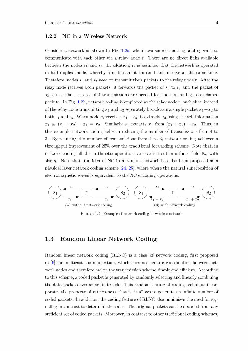
1.2.2 NC in a Wireless Network
Consider a network as shown in Fig. 1.2a, where two source nodes s1 and s2 want to
communicate with each other via a relay node r. There are no direct links available
between the nodes s1 and s2. In addition, it is assumed that the network is operated
in half duplex mode, whereby a node cannot transmit and receive at the same time.
Therefore, nodes s1 and s2 need to transmit their packets to the relay node r. After the
relay node receives both packets, it forwards the packet of s1 to s2 and the packet of
s2 to s1. Thus, a total of 4 transmissions are needed for nodes s1 and s2 to exchange
packets. In Fig. 1.2b, network coding is employed at the relay node r, such that, instead
of the relay node transmitting x1 and x2 separately broadcasts a single packet x1 +x2 to
both s1 and s2. When node s1 receives x1 + x2, it extracts x2 using the self-information
x1 as (x1 + x2) − x1 = x2. Similarly s2 extracts x1 from (x1 + x2) − x2. Thus, in
this example network coding helps in reducing the number of transmissions from 4 to
3. By reducing the number of transmissions from 4 to 3, network coding achieves a
throughput improvement of 25% over the traditional forwarding scheme. Note that, in
network coding all the arithmetic operations are carried out in a finite field Fq, with
size q. Note that, the idea of NC in a wireless network has also been proposed as a
physical layer network coding scheme [24, 25], where where the natural superposition of
electromagnetic waves is equivalent to the NC encoding operations.
x1
x2
s1 s2rx2
x1
(a) without network coding
x1 + x2
x2
s1 s2rx1
x1 + x2
(b) with network coding
Figure 1.2: Example of network coding in wireless network
1.3 Random Linear Network Coding
Random linear network coding (RLNC) is a class of network coding, first proposed
in [6] for multicast communication, which does not require coordination between net-
work nodes and therefore makes the transmission scheme simple and efficient. According
to this scheme, a coded packet is generated by randomly selecting and linearly combining
the data packets over some finite field. This random feature of coding technique incor-
porates the property of ratelessness, that is, it allows to generate an infinite number of
coded packets. In addition, the coding feature of RLNC also minimizes the need for sig-
naling in contrast to deterministic codes. The original packets can be decoded from any
sufficient set of coded packets. Moreover, in contrast to other traditional coding schemes,
Chapter 1. Introduction 5
RLNC is capable to adapt to any transmission rate on the fly. Because of these fea-
tures, RLNC is easy to implement and is considered as a suitable technique for dynamic
topologies and varying connections. Thus, RLNC is a powerful method for node coop-
eration, in particular for broadcast communication, and in distributed networks, where
nodes cannot easily coordinate the routing of information through the network. Further-
more in [6], it has been proved that RLNC due to its inherent randomness achieves the
multicast capacity in a distributed fashion. In energy-constraint wireless networks, such
as sensor networks, the communicating nodes are typically battery powered and have a
limited energy budget. The improvement of the network lifetime without a reduction
in network reliability is a major challenge. RLNC can decrease the number of distinct
packet transmissions in a network and minimize or eliminate packet retransmissions due
to poor channel conditions [6]. Consequently, RLNC has the potential to both improve
energy efficiency [26] and reduce the overall latency in a network [27], which effectively
leads to an increase in the lifetime of the network.
1.3.1 RLNC Encoding and Decoding
The encoding process is employed on packets/symbols, where a packet could be com-
posed of multiple symbols. These packets could be either obtained after dividing the
information at the source node or could be packets of different information flows received
at intermediate nodes. In order to understand the encoding process, let us assume that
there are m packets {x1, x2, . . . , xm} which need to be encoded using RLNC. A coded
packet yi can be obtained by simple vector multiplication, as follows
yi=[c1,i, c2,i, . . . , cm,i
]x1
x2
...
xm
(1.1)
where, [c1,i, c2,i, . . . , cm,i] is the coding vector whose elements (coding coefficients) are
selected independently at random over the finite field Fq with size q. In this way, we can
generate m+ κ coded packets and coding vectors, where κ is any number of redundant
packets. Thus, the encoding process can, in theory, generate an infinite number of coded
packets. However, due to the random selection of coding coefficients there is a non-zero
probability that some of the coding vectors are linearly dependent and the corresponding
coded packets cannot contribute to the decoding process. Before transmitting a coded
packet into a network, the coding vector is appended to the associated coded packet,
as described in [28] and shown in Fig 1.3. Where, the header may contain information
or data associated to other layers of protocol stack, required for a packet to reach its
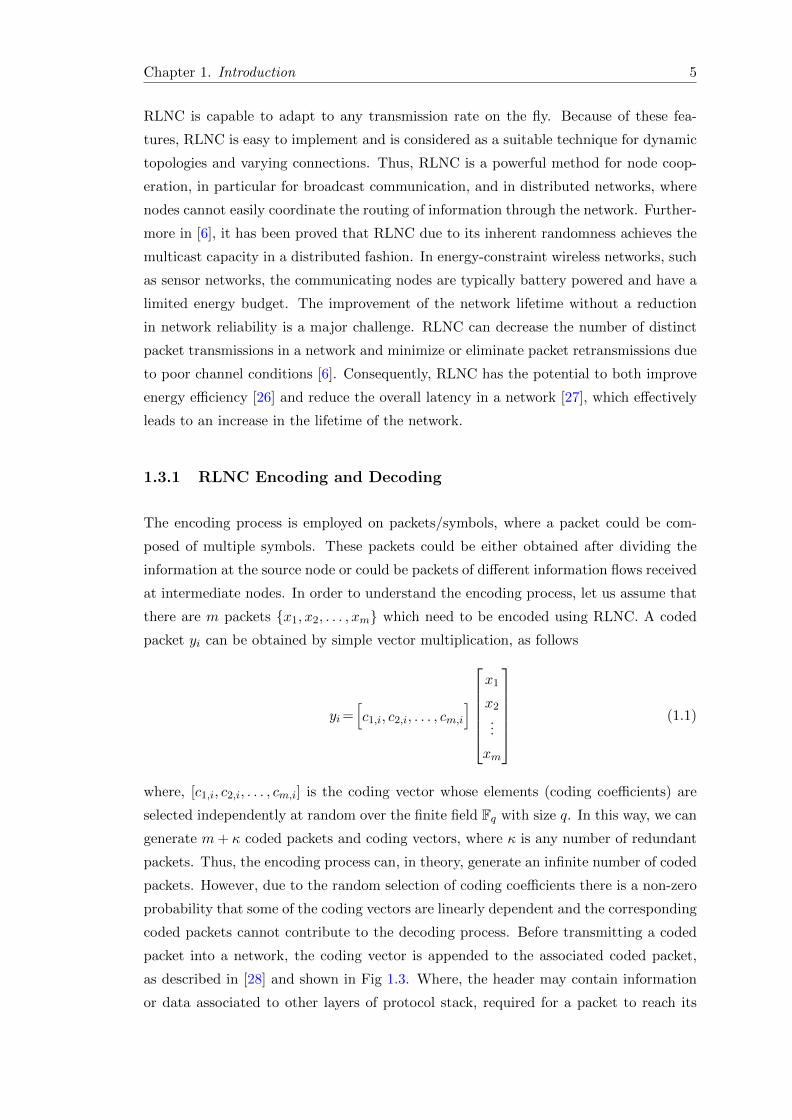
Chapter 1. Introduction 6
intended destination. A sink node after receiving a transmitted packet, extracts both
Header Coding vector Coded packet
Figure 1.3: Structure of transmitted coded packet
the coded packet and the coding vector, and stores them into two separate matrices that
could be termed as payload matrix and decoding matrix respectively, provided that the
coding vector is linearly independent. In order for a sink to decode m original packets, it
must collect at least m coded packets with linearly independent coding vectors. Finally,
the sink node employs Gaussian elimination on the decoding matrix augmented with
the payload matrix to decode the packets.
1.3.2 RLNC Example
s
r2 r3
d
r1
x1 x2 x3x1 x2 x3
x1 x2 x3
x1 x2 x3 x1 x3
x1 x2
x1 x2 x3
(a) Without RLNC
s
r2 r3
d
r1
x1 x2 x3x1 x2 x3
x1 x2 x3
y11 y12 y13 y31 y32y21 y22
x1 x2 x3
(b) With RLNC
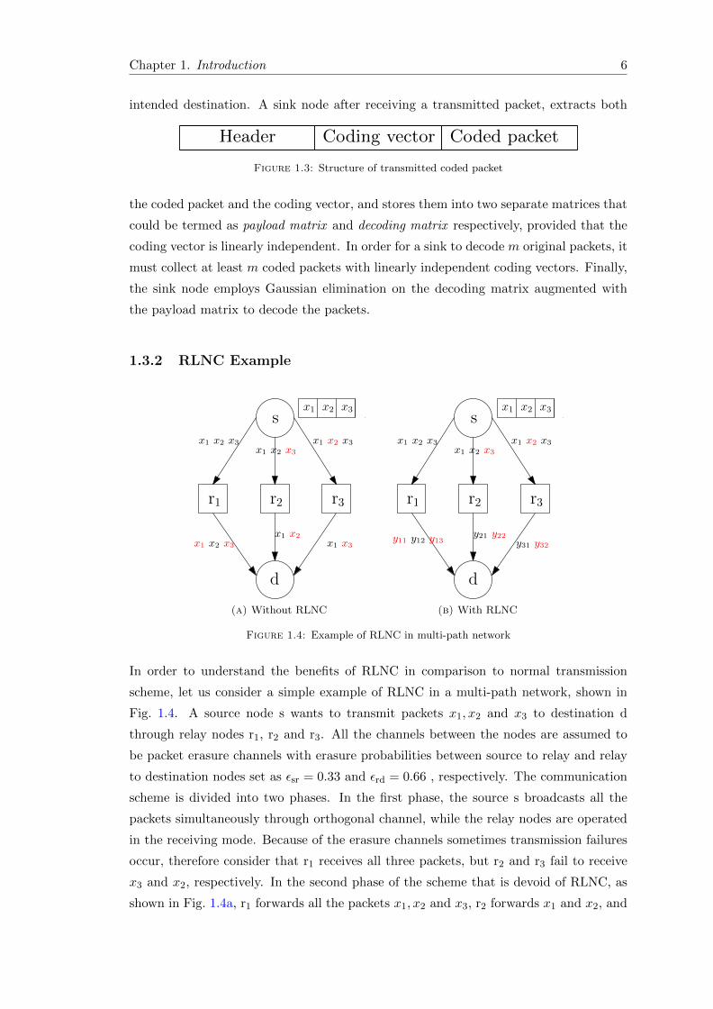
Figure 1.4: Example of RLNC in multi-path network
In order to understand the benefits of RLNC in comparison to normal transmission
scheme, let us consider a simple example of RLNC in a multi-path network, shown in
Fig. 1.4. A source node s wants to transmit packets x1, x2 and x3 to destination d
through relay nodes r1, r2 and r3. All the channels between the nodes are assumed to
be packet erasure channels with erasure probabilities between source to relay and relay
to destination nodes set as εsr = 0.33 and εrd = 0.66 , respectively. The communication
scheme is divided into two phases. In the first phase, the source s broadcasts all the
packets simultaneously through orthogonal channel, while the relay nodes are operated
in the receiving mode. Because of the erasure channels sometimes transmission failures
occur, therefore consider that r1 receives all three packets, but r2 and r3 fail to receive
x3 and x2, respectively. In the second phase of the scheme that is devoid of RLNC, as
shown in Fig. 1.4a, r1 forwards all the packets x1, x2 and x3, r2 forwards x1 and x2, and
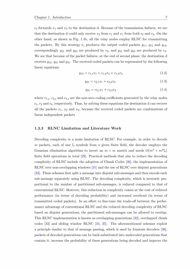
Chapter 1. Introduction 7
r3 forwards x1 and x3 to the destination d. Because of the transmission failures, we see
that the destination d could only receive x2 from r1 and x1 from both r2 and r3. On the
other hand, as shown in Fig. 1.4b, all the relay nodes employ RLNC for transmitting
the packets. By this strategy r1 produces the output coded packets y11, y12 and y13,
correspondingly y21 and y22 are produced by r2, and y31 and y32 are produced by r3.
We see that because of the packet failures, at the end of second phase, the destination d
receives y12, y21 and y31. The received coded packets can be represented by the following
linear equations:
y12 = c1,1x1 + c1,2x2 + c1,3x3 (1.2)
y21 = c2,1x1 + c2,2x2 (1.3)
y31 = c3,1x1 + c3,3x3 (1.4)
where c1,j , c2,j and c3,j are the non-zero coding coefficients generated by the relay nodes
r1, r2 and r3, respectively. Thus, by solving these equations the destination d can recover
all the packets x1, x2 and x3, because the received coded packets are combinations of
linear independent packets
1.3.3 RLNC Limitation and Literature Work
Decoding complexity is a main limitation of RLNC. For example, in order to decode
m packets, each of size L symbols from a given finite field, the decoder employs the
Gaussian elimination algorithm to invert an m × m matrix and needs O(m3 + m2L)
finite field operations in total [29]. Practical methods that aim to reduce the decoding
complexity of RLNC include the adoption of Chunk Codes [30], the implementation of
RLNC over non-overlapping windows [31] and the use of RLNC over disjoint generations
[32]. These schemes first split a message into disjoint sub-messages and then encode each
sub-message separately using RLNC. The decoding complexity, which is inversely pro-
portional to the number of partitioned sub-messages, is reduced compared to that of
conventional RLNC. However, this reduction in complexity comes at the cost of reduced
performance (in terms of decoding probability) and increased overhead (in terms of
transmitted coded packets). In an effort to fine-tune the trade-off between the perfor-
mance advantage of conventional RLNC and the reduced decoding complexity of RLNC
based on disjoint generations, the partitioned sub-messages can be allowed to overlap.
This RLNC implementation is known as overlapping generations [32], overlapped chunk
codes [33] and sliding window RLNC [34, 35]. The aforementioned schemes exploit
a principle similar to that of message passing, which is used by fountain decoders [36];
packets of decoded generations can be back-substituted into undecoded generations that
contain it, increase the probability of these generations being decoded and improve the
Chapter 1. Introduction 8
overall throughput. In order to further reduce both the decoding complexity and the
overhead while maintaining the delay performance, the concept of sparse RLNC within
each generation as well as a feedback mechanism to control the amount of overlap be-
tween generations were proposed in [29, 37].
1.4 RLNC Applications
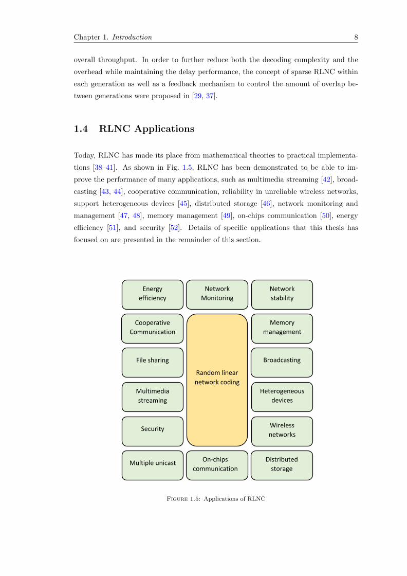
Today, RLNC has made its place from mathematical theories to practical implementa-
tions [38–41]. As shown in Fig. 1.5, RLNC has been demonstrated to be able to im-
prove the performance of many applications, such as multimedia streaming [42], broad-
casting [43, 44], cooperative communication, reliability in unreliable wireless networks,
support heterogeneous devices [45], distributed storage [46], network monitoring and
management [47, 48], memory management [49], on-chips communication [50], energy
efficiency [51], and security [52]. Details of specific applications that this thesis has
focused on are presented in the remainder of this section.
Wireless
networks
Distributed
storage
Multimedia
streaming
File sharing
Network
Monitoring
Memory
management
Multiple unicast
Heterogeneous
devices
Broadcasting
Energy
efficiency
Network
stability
Cooperative
Communication
Security
On-chips
communication
Random linear
network coding
Figure 1.5: Applications of RLNC
Chapter 1. Introduction 9
1.4.1 RLNC for Heterogeneous Devices and Broadcast Communica-
tion
RLNC can be used to facilitate heterogeneous devices with different processing power,
size and storage limitations. In order to accommodate a diverse set of receiving devices,
the data that are about to be transmitted by a base station or access point can be
divided into priority layers, which are encoded using RLNC that offers Unequal Error
Protection (UEP) [31, 53]. The priority layers usually consist of a base layer and multiple
enhancement layers. The base layer is responsible for providing a basic level of service,
suitable for all types of devices with small storage and limited processing power. On
the other hand, the enhancement layers contain data which can improve the quality
of service. Thus, access to all or as many as possible layers offers a high quality of
service. This layered structure of RLNC has fitted well into different applications. For
example, in [54] as Prioritized Random Linear Coding (PRLC) for layered data delivery
from multiple servers, in [44] as UEP RLNC for wireless layered video broadcasting and
in [43] as Expanding Window-RLNC (EW-RLNC) for multimedia multicast services
based on the H.264/SVC standard.
1.4.2 Random Linear Network Coded Cooperation
RLNC has attracted substantial research efforts due to its appealing benefits in coop-
erative communications. Several works in the literature have exploited Random Linear
Network Coded Cooperation (RLNCC) for achieving reliability, energy efficiency,and
diversity gain. For example in [55], RLNC-based cooperation was employed in coop-
erative compressed sensing for achieving energy efficiency and robustness against link
failures. In [56, 57], network coded cooperation was employed to achieve maximum
diversity gain. Cooperative communication with deterministic and random network
coding schemes were studied in [58], where it has been demonstrated that both schemes
outperform conventional cooperation in terms of diversity-multiplexing tradeoff. More-
over in [59] and [60], the authors proposed an analytical framework to characterize the
performance of an RLNCC system in terms of bounds of decoding failure probability.
1.4.3 RLNC for Secure Communication
One of the elegant qualities of RLNC is its inherent nature of security. Therefore, the
problem of achieving secure communication in systems employing network coding has
recently attracted the attention of the research community in wireless networks. Ning
Chapter 1. Introduction 10
and Yeung [61] first formulated the concept of secure network coding, which avoids in-
formation leakage to a wiretapper. They imposed a security requirement, that is, the
mutual information between the source symbols and the symbols received by the wire-
tapper must be zero for secure communication. Based on a well-designed precoding
matrix, Wang et al. [62] proposed a secure broadcasting scheme with network coding to
obtain perfect secrecy. Probabilistic weak security for linear network coding was pre-
sented in [63], which devised network coding rules that can improve security depending
on the adopted field size, the number of transmitted symbols and the ability of the
attacker to eavesdrop on one or more independent channels. Moreover, the intercept
probability of fountain coding, which is equivalent to random linear network coding
for wireless broadcast applications, was formulated in [64] and exploited for industrial
wireless sensor networks in [52].
1.4.4 RLNC Integrated with Opportunistic Relaying and Intentional
Jamming
The dynamic nature of the wireless medium often introduces problems to the operation of
wireless networks, which are related to node connectivity, communication reliability and
robustness [65]. Methods that can ameliorate the side effects of wireless environments
include opportunistic relaying and node cooperation [66]. For example, opportunistic
relaying was proposed as an alternative to distributed space-time relaying; it achieves
full diversity gain [67] but can also improve energy efficiency [68, 69]. Opportunistic
routing based on cooperative forwarding was presented in [70] to combat errors and
link failures in sensor networks. Multi-phase node cooperation for indoor industrial
monitoring was described in [71] as a means to reduce energy consumption. Moreover,
an experimental study of selective cooperative relaying was provided in [72]. Advantages
from using opportunistic relaying with network coding in two-way relay communications
have been reported in [73–75].
Even though opportunistic relaying and RLNC have the potential to improve energy
efficiency and link reliability, the broadcast nature of the wireless medium renders data
transmission to an authorized destination vulnerable to eavesdropping. The secure de-
livery of confidential data is important for many applications, for example, sharing of
sensitive information or key distribution. In order to achieve secrecy and privacy, many
cryptographic schemes are widely designed and adopted on the higher layers of the pro-
tocol stack, while assuming the error free communication at the physical layer. However,
these methods usually require high computational power, and typically assume limited
computing power for the eavesdroppers. Against this background, Physical-layer secu-
rity (PLS) has emerged as a major research topic in recent years, and has been proposed
Chapter 1. Introduction 11
as an alternative to achieve perfect resilience against eavesdropping attacks without re-
quiring special key distribution and complex encryption/decryption algorithm [76, 77].
The core idea behind this paradigm is to exploit the dynamic nature of radio channel,
such as fading and noise, for maximizing the uncertainty concerning the source messages
at the eavesdropper [78, 79]. These properties are traditionally interpreted as impair-
ments, but PLS take advantage of these properties for achieving secrecy in wireless
transmission. PLS was first introduced in [80], where the wiretap channel was charac-
terised as the fundamental element to protect information at the application layer. In
this seminal work, the security is evaluated by establishing a metric called secrecy ca-
pacity as the maximum rate of transmission at which the information is considered to be
secure without being interpreted by an eavesdropper. Later the subsequent result was
employed to the broadcast channel in [79] and basic Gaussian channel in [81]. Moreover
in the literature, several techniques are proposed for enhancing the PLS, including: se-
cure on-off power allocation designs [82], secrecy enhancing channel coding scheme [83],
and beamforming/precoding and artificial interference-aided techniques relying on mul-
tiple antennas [84]. Furthermore, PLS can be easily integrated into wireless networks
that combine opportunistic relaying with cooperative communication [85–87]. For exam-
ple in [85], a relay selection metric that utilizes knowledge of the relay-to-eavesdropper
instantaneous channel conditions was presented and the network performance was eval-
uated in terms of the secrecy outage probability. Opportunistic relay selection protocols
in the presence of multiple eavesdroppers were studied in [86]. The effect of single-
relay and multi-relay selection on the performance of physical layer security in wireless
networks was investigated in [87] and security-reliability tradeoffs were identified us-
ing comparisons between the intercept probability and the outage probability of direct
transmission. On the other hand, jamming is a well-known PLS approach to enhance
the quality of security in wireless transmissions [88, 89]. In this scheme, additional in-
terference signals are transmitted to confuse the potential eavesdroppers or to degrade
the channel’s quality of unintentional receivers. These interference signals can be intro-
duced by embedding them in the intended signals, which are also referred as artificial
noise approach in the literature [90]. Moreover, cooperative jamming scheme has at-
tained significant attention in the literature [91–94], and has become an effective way
for improving the achievable secrecy rate. In this technique, a friendly jammer node
aims to disturb the eavesdroppers and protect the legitimate users. For example, coop-
erative jamming strategy is provided in [91] for improving the secrecy rate. In addition,
joint relay-and-jammer selection techniques were proposed in [92] to increase the secrecy
capacity in wireless networks, whereas suboptimal relay selection and suboptimal joint
relay-and-jammer selection protocols were compared in [93].
The main objective of PLS techniques is to increase the secrecy rate between the source
Chapter 1. Introduction 12
and the destination, while ensuring that the transmitted information cannot be accessed
by an eavesdropper. Strict information-theoretic security is achieved if and only if the
mutual information between the packets available to an eavesdropper and the source
packets is zero [61]. The performance of PLS schemes is often measured by the secrecy
capacity, which is the maximum rate for reliable and perfectly secure communication,
and the secrecy outage probability, which is the probability that secure communication
will fail. However, these two metrics are used to optimize the transmission rate, so that
the legitimate destination will fully recover the transmitted data with perfect secrecy. If
information-theoretic secrecy cannot be achieved, the secrecy capacity and the secrecy
outage probability do not provide any insight into the likelihood of an eavesdropper
recovering only a fraction of the transmitted confidential information. To the best of
our knowledge, only few studies that exploit the properties of RLNC in PLS are available.
For example, fountain coding based secure wireless communication was analyzed in [64],
and to enhance the secrecy of cooperative transmissions in sensor networks, fountain-
coding aided cooperative relaying with jamming was proposed in [52].
1.5 Overview and Contributions of Thesis
This thesis is concerned with the development of probabilistic frameworks to evaluate
and characterize the performance of RLNC based communications. More specifically,
the problems which are considered in this thesis provide answers to the following main
questions:
• Research Question 1 (RQ1): How can we exploit random matrix theory over
finite fields to formulate and characterize the performance of RLNC with layered
structures and tunable sparsity?
• Research Question 2 (RQ2): How can we develop probabilistic models to evaluate
the performance of RLNCC and design a framework which integrates the benefits
of physical layer multiplexing using the emerging NOMA and RLNCC?
• Research Question 3 (RQ3): How can we evaluate and quantify the intrinsic
security level provided by RLNC, and how can we design a cross layer security
scheme which exploits the intrinsic security of RLNC on top of physical layer
security techniques with minimum effect on reliability?
In particular, research question RQ1 deals with the rank of random matrices over fi-
nite fields with adjustable tunable level of sparsity for the purpose of addressing the
decoding complexity of RLNC, supporting heterogeneous devices and point-to-point or
Chapter 1. Introduction 13
point-to-multipoint prioritized communication. On the other hand, RQ2 mainly deals
with tunable sparse RLNC and its applications for opportunistic coded cooperation.
RQ3 deals with the resilience of RLNC against eavesdropping, and also deals with the
combination of RLNC, and relay and jammer selection techniques to discourage eaves-
dropping and support reliability.
1.5.1 Thesis Structure and Organization
Characterising the performance of RLNC for reliable and secure
communication
Thesis goal
Practical
issues
Channel
models
Performance
metrics
Decoding
success/failure
probability
Throughput and delay
Intercept probability
RLNC with layered structures and tuneable
sparsity Chapter 2—RQ1
Packet erasure
RLNCC, RLNCC combined with NOMA
Chapter 3—RQ2
Packet erasure/Block fading
Intrinsic nature of RLNC and cross layer security
Chapter 4—RQ3
Packet erasure/Block fading
Figure 1.6: Thesis Flowchart
Fig. 1.6 exhibits the flowchart of the thesis structure. Chapter 2 tackles the research
question RQ1, by focusing on random block matrices over finite fields and investigating
different matrix structures, which model the encoding process of layered structures of
RNLC schemes. In order to address the decoding complexity of RLNC and support low
power devices, these structures also allow to adjust the sparsity level of encoding. More
specifically in this chapter, we employ fundamental expressions of random matrix the-
ory over finite fields and develop a mathematical framework for the considered matrix
structures. The proposed framework can be used to accurately characterize the prob-
ability that a receiver will successfully decode transmitted data or layers of a service.
Numerical results and discussions are provided.
The results in this chapter have been presented in the following journal paper:
J1: A. S. Khan and I. Chatzigeorgiou, “A Framework for the Analysis of Network-
Coded Schemes Characterized by Random Block Matrices”, IEEE Transactions on Wire-
less Communications, under preparation.
Chapter 1. Introduction 14
Chapter 3 attempts to answer the research question RQ2, by studying three different
network models. Here, we first consider a relay assisted network with two source nodes
and a single destination node, where source nodes employ intra-session RLNC and the
relay node employs inter-session RLNC for coded cooperation. The performance of the
network is characterized by the probability of decoding success at the destination node.
Closed form mathematical expressions are derived to evaluate the performance, and
at the end, results and discussions are provided. Secondly, we consider a multi-source
multi-relay network, where only relay nodes employ RLNC for coded cooperation. The
performance of the network is characterized by the decoding failure probability. Exact
theoretical expressions to evaluate this probability is still an open problem. However in
this chapter, we derive mathematical closed form expressions to evaluate tighter upper
and lower bounds to the failure probability. Simulation results and discussions are pro-
vided to exhibit the tightness of the derived expressions and characterize the network
performance. Thirdly, we consider a multiple relay network with two source groups
and two destination nodes, and propose a framework which integrates the advantages
of RLNCC and NOMA based communication. Theoretical closed form expressions are
derived to evaluate the network performance mainly in terms of throughput and suc-
cessful decoding probability at the destination nodes. Simulation results and discussions
are provided to demonstrate the benefits of NOMA based RLNCC as compared to the
conventional OMA based communication.
The results in this chapter have been presented in the following conference and journal
publications:
C1: A. S. Khan and I. Chatzigeorgiou, “Performance analysis of random linear network
coding in two-source single-relay networks”, in Proc. IEEE International Conference on
Communications Workshops (ICC), Workshop on Cooperative and Cognitive Networks,
London, United Kingdom, June 2015.
J2: A. S. Khan and I. Chatzigeorgiou, “Improved bounds on the decoding failure
probability of linear NC over multi-source multi-relay networks”, IEEE Communications
Letters, vol. 20, no. 10, pp. 2035-2038, Oct. 2016.
J3: A. S. Khan and I. Chatzigeorgiou, “Non-Orthogonal Multiple Access Combined
With Random Linear Network Coded Cooperation”, IEEE Signal Processing Letters,
vol. 24, no. 9, pp. 1298-1302, Sept. 2017.
Chapter 4 addresses the research question RQ3, by presenting two different network
models where RLNC is employed for secure communications. In this chapter, we first
consider a simple point-to-point network with conventional characters: Alice, Bob and
a passive eavesdropper. Where, Alice exploits RLNC for secure communication to Bob.
Feedback and without feedback protocols are considered, and the secrecy of communi-
cation is evaluated by deriving the exact close form expression of intercept probability
Chapter 1. Introduction 15
corresponding to each protocol. Moreover, an optimization model is presented for further
improving the network security. All the analyses are supported by simulation results and
discussions. Secondly, a multi-relay network is considered to integrate the advantages
of RLNC and physical layer security techniques. In particular, we consider relay/jam-
mer selection techniques for physical layer security and RLNC at the application layer
for self-encryption of data. Closed form outage expressions are derived corresponding
to each relay/jammer selection technique. Furthermore, network security is accurately
quantified by developing a framework which characterizes the probability of the eaves-
dropper intercepting a sufficient number of coded packets and partially or fully decoding
the confidential data. Simulation results and discussions are presented to support the
analysis and to exhibit a tradeoff between reliability and security corresponding to each
relay/jammer selection technique.
The results in this chapter have been presented in the following journal publications:
J4: A. S. Khan, A. Tassi and I. Chatzigeorgiou, “Rethinking the intercept probability
of random linear network coding”, IEEE Communications Letters, vol. 19, no. 10, pp.
1762-1765, October 2015.
J5: A. S. Khan and I. Chatzigeorgiou, “Opportunistic relaying and random linear
network coding for secure and reliable communication”, IEEE Transactions on Wireless
Communications, accepted with minor revisions.
Chapter 5 summarizes the thesis and provides the general conclusions drawn from each
chapter. In addition, some possible research areas are also presented as an extension to
the research presented in the thesis.
Chapter 2
A Framework for the Assessment
of Network Coding Techniques
Characterized by Random Block
Matrices
Random matrix theory (RMT) was first introduced by Wishart [95] in 1928. From its
inception, numerous fields of science, engineering and statistics have been heavily influ-
enced. Nowadays it is a key subject in topics of information theory, wireless communica-
tions, graph theory, signal processing, probability, multivariate statistics, combinatorics,
statistical physics and quantum communication. Two fundamental reasons for the ever
growing success of RMT can be identified. Firstly, RMT techniques offer remarkably
precise predictions of analytical computations that grow to infinity in the context they
are modeling. Secondly, RMT outcomes can be applied on any kind of random matrix,
as long as the entries are independent and can be formalized in a given environment
[96, 97]. This implies that RMT does not depend on the probability distribution that
defines the matrix entries, but depends only on the invariant properties of their dis-
tribution [98]. Thus, RMT is a valuable tool for modeling a large number of complex
mathematical and physical problems.
The modeling and performance evaluation of information processing techniques, includ-
ing random linear network coding RLNC, relies on RMT over the finite fields. Practical
methods that are designed to reduce decoding complexity or introduce unequal error
protection properties, add constraints to the entries of matrices that characterize RLNC
schemes. These constraints permit only entries within particular blocks of an RLNC ma-
trix to take random values from a finite field, while the remaining entries are set to zero.
16
Chapter 2. A Framework for the Assessment of Network Coding Techniques 17
This chapter considers random block matrices and presents a mathematical framework
for the enumeration of full-rank matrices that contain blocks of random entries arranged
in a diagonal, lower-triangular or tri-diagonal structure. The derived expressions are
then used to model the probability that a receiver will successfully decode a source mes-
sage or layers of a service, when RLNC based on non-overlapping, expanding or sliding
generations is employed. In particular, this framework is suitable for the study of sys-
tems employing random linear network coding to broadcast or multicast information,
including content streaming and data distribution.
This chapter has been organized as follows: Section 2.1 introduces fundamental expres-
sions for the rank of random matrices over finite fields. Section 2.2 treats partitioned
random matrices as a special case of random block matrices and derives an equivalent
formula for the number of full-rank matrices. Section 2.3 investigates the aforementioned
structures of random block matrices and obtains theoretical expressions for the full-rank
of each matrix. Section 2.4 briefly describes three existing RLNC implementations and
establishes links between the previously derived theoretical formulas and the decoding
probability of each RLNC scheme. Results are discussed in Section 2.5, and finally the
contributions in this chapter are summarized in Section 2.6.
2.1 Fundamental Preliminary Expressions
Finite or Galois fields have been receiving steady attention because of their applications
in many cryptographic techniques and error correcting codes. Let M ∈ Fn×mq be a
matrix that has been sampled uniformly at random from the set of all n ×m matrices
with elements from Fq, where q is a prime power pr (such that, p is a prime number
and r is a positive integer) [99]. Matrix M is said to be a full-rank matrix if it has rank
min(n,m) or, equivalently, min(n,m) rows of M are linearly independent. For n ≥ m,
the number of full-rank n×m matrices can be computed as follows [100]
γ(n,m) =
∏m−1i=0 (qn − qi), if m ≥ 1
1, if m = 0.(2.1)
The probability that a matrix M is a full-rank matrix can be obtained by dividing
γ(n,m) by qnm, which represents the total number of matrices in Fn×mq , that is,
P (n,m) =γ(n,m)
qnm. (2.2)
Chapter 2. A Framework for the Assessment of Network Coding Techniques 18
If the rank of M is r, where 0 ≤ r ≤ min(n,m), the number of all matrices of rank r in
Fn×mq , is given by [101, 102]
γr(n,m) =
[n
r
]q
γ(m, r) (2.3)
where the term[nr
]q
specifies the number of r-dimensional subspaces of an n-dimensional
vector space over the finite field Fq. It is widely known as the Gaussian or q-binomial
coefficient [103] and is defined as
[n
r
]q
=
(1−qn)(1−qn−1)...(1−qn−r+1)
(1−q)(1−q2)...(1−qr) , if r ≤ n
0, if r > n.(2.4)
The q-binomial coefficient can also be expressed as the ratio of the number of full-rank
matrices in Fn×rq to the number of full-rank matrices in Fr×rq [102], that is,[n
r
]q
=γ(n, r)
γ(r, r). (2.5)
The probability of M having rank r can be obtained by dividing γr(n,m) by the total
number of n×m matrices as follows
Pr(n,m) =γr(n,m)
qnm. (2.6)
The fundamental expressions presented in this section will be invoked in the derivation
of proofs in the following sections.
2.2 Partitioning of Random Matrices
Even though the formula that computes the number of n×m full-rank random matrices
is derived in [100] as presented in (2.1), an exact equivalent expression that treats a
random matrix as the concatenation of sub-matrices is also of interest and will be derived
in this section. The derived expression will then be adapted to specific structures of
random block matrices, which can be used in the performance modelling of network-
coded systems.
Before we proceed with the proof of a lemma, which will lead us to the main proposition
of this section, we first introduce some additional notation. If M1, . . . ,ML are matrices
having the same number of columns, then (M1; . . . ; ML) denotes the matrix obtained
by the vertical concatenation of the L matrices or, equivalently, by appending Mi+1 to
the bottom of Mi for i = 1, . . . , L− 1.
Chapter 2. A Framework for the Assessment of Network Coding Techniques 19
Lemma 2.1. Let M = (M1; M2) ∈ F(n1+n2)×mq be a random matrix obtained by verti-
cally concatenating M1 ∈ Fn1×mq and M2 ∈ Fn2×m
q , where n1 +n2 ≥ m. The number of
combinations of all realisations of matrices M1 and M2 that result in a full-rank random
matrix M is equal to
γ(n1+n2, m) =∑r1
γr1(n1,m)γ(n2, m−r1)qn2r1 (2.7)
where max(0,m− n2) ≤ r1 ≤ min(n1,m).
Proof. Matrix M is a full-rank matrix iff it contains m linearly independent columns.
Let r1 columns of M1 be linearly independent. The corresponding columns of M2 can
take qn2r1 possible values, while the remaining m− r1 columns of M2 can be selected in
γ(n2,m− r1) possible ways to give a full-rank n2 × (m− r1) submatrix. Therefore, the
number of matrices M having m linearly independent columns is equal to the number
of all possible matrices M1 of rank r1 given by γr1(n1,m), multiplied by the number of
all possible matrices M2 of rank m − r1 given by γ(n2,m − r1)qn2r1 , summed over all
valid values of r1. A proof, which analytically demonstrates that the right-hand side
of (2.7) is equal to the right-hand side of (2.1) for n = n1 + n2, is presented in the
Appendix A.
Proposition 2.2. Let L random matrices M1, . . . ,ML, where Mi ∈ Fni×mq for 1 ≤ i ≤L, be vertically concatenated in order to generate M =(M1; M2; . . . ; ML)∈Fn×mq , where
n = n1 + . . .+ nL. Equivalently, we can write
M=
M1
M2
...
ML
.
The number of all possible matrices M1, M2, . . . ,ML that result in a full-rank matrix
M is equal to
γ(n,m)=∑r1
γr1(n1,m) γ(n−n1, m−r1) q(n−n1)r1 (2.8)
in recursive form, or
γ(n,m)=∑r1
· · ·∑rL−1
L∏i=1
γri(ni,m−Ri−1)q∑L−1k=1 nk+1Rk (2.9)
in non-recursive form, where:
Rk = r1 + r2 + . . .+ rk and R0 = 0 for k = 0,
n = n1 + n2 + . . .+ nL ≥ m
Chapter 2. A Framework for the Assessment of Network Coding Techniques 20
and ri, for i = 1, . . . , L− 1, takes values in the range
ri ≥ max(0,m−Ri−1 −∑L
j=i+1 nj) and
ri ≤ min(ni,m−Ri−1), while rL =m−RL−1 for i= L.
Proof. The expression (2.8) is a recursive formulation of γ(n,m) in terms of γ(n−n1, m−r1)
given that the vertical concatenation of L matrices can be viewed as the concatenation
of two matrices, that is, M1 and (M2; M3; . . . ; ML) or, equivalently,
(M1; M2; . . . ; ML) ≡ (M1; (M2; M3; . . . ,ML)).
The non-recursive expression (2.9) can be derived from (2.8) if Lemma 2.1 is repeatedly
applied on γ(n− n1, m− r1) in (2.8), given that argument n − n1 can be written as
n2 + . . . + nL. This process is equivalent to expressing the vertical concatenation of L
matrices as follows
(M1; . . . ;ML)≡(M1;(M2;(M3; . . . ;(ML−1;ML)))).
Note that (2.3) has been used to express the number of both full-rank and rank-deficient
matrices because γri(ni,m−Ri−1) in (2.9) reduces to γ(ni,m−Ri−1) for ri = m−Ri−1.
This section established that expression (2.1), which provides the number of full-rank
n ×m random matrices, can also take the form of (2.9), which partitions the random
matrix into L sub-matrices and counts all possible combinations of each sub-matrix
having a particular rank. The advantage of (2.9) over (2.1) is that it can be readily
adapted to random block matrices, as will become evident in the following section.
2.3 Structures of Random Block Matrices
Whereas entries of a random matrix over a finite field Fq can take any of the q available
values with equal probability, there exist cases where only a constrained number of
entries can take values from Fq while the remaining entries are set to zero. We refer to
matrices that contain blocks of random entries as random block matrices and we focus
on the following general matrix structure in this chapter:
M=
M1(n1, s1 : e1)
M2(n2, s2 : e2)...
ML(nL, sL : eL)
.
Chapter 2. A Framework for the Assessment of Network Coding Techniques 21
According to this structure, the n×m matrix M is the vertical concatenation of matrices
Mi(ni, si :ei) of dimensions ni×m, for i = 1, . . . , L. Parameters si and ei signify the first
and last columns of an ni × (ei − si + 1) random sub-matrix within Mi. The remaining
elements of Mi are equal to zero. Depending on the values of si and ei, columns of Mi
that contain random elements will be connected to columns of matrices above or below
Mi that contain either random elements or zeros. This section will study three spe-
cific structures of random block matrices, namely Block Diagonal (BD) matrices, Block
Lower-Triangular (BLT) matrices and Block Tri-Diagonal (BTD) matrices, and will de-
rive exact expressions for the number of full-rank matrices in each case. The examples
of random block matrices with the considered structures are exhibited in Fig. 2.1.
(a) Block diagonal (BD) (b) Block lower-triangular(BLT)
(c) Block tri-diagonal(BTD)
Figure 2.1: Examples of 25 × 20 random block matrices, which have been constructed byvertically concatenating three matrices. Random elements are depicted by ‘�’, while zero-
valued entries are represented by ‘�’.
2.3.1 Block Diagonal (BD) Matrices
Consider an n×m matrix M with the following structure
M=
M1(n1, 1 : e1)
M2(n2, e1 + 1 : e2)...
ML(nL, eL−1 + 1 : m)
where n = n1 + . . . + nL, si = ei−1 + 1 for i = 2, . . . , L, while s1 = 1 and eL = m. An
example of a BD matrix for L = 3 is presented in Fig. 2.1a.
If mi = ei−ei−1 denotes the number of columns in Mi that consist of random elements,
we can infer that the n×m matrix M contains L random sub-matrices along its diagonal,
each of dimensions ni×mi, as shown in Fig. 2.1a. Observe that if a column of Mi consists
of random elements, this column is connected to columns of matrices below or above
Mi that always contain zeros. Consequently, the problem of computing the number of
Chapter 2. A Framework for the Assessment of Network Coding Techniques 22
full-rank matrix realizations of M can be reduced to a set of independent problems, each
associated to the number of full-rank ni×mi random sub-matrices. This implies that M
is a full-rank matrix only if each ni×mi matrix Mi, for i = 1, . . . , L, has a full rank or,
using mathematical notation, if ni ≥ mi, m1 + · · ·+mL = m and ri = mi. Substituting
these conditions into (2.9) reduces the general expression of Proposition 2.2 into the
following well-known relationship [43]
γBD(M) =L∏i=1
γ(ni,mi) (2.10)
Therefore, the structure of BD matrices requires a reduced version of (2.9) to compute
the number of full-rank matrices. Expression (2.9) can also be adjusted for the case of
BLT matrices, as will be discussed in the following section.
2.3.2 Block Lower-Triangular (BLT) Matrices
The general structure of an n×m BLT matrix M is
M=
M1(n1, 1 : e1)
M2(n2, 1 : e2)...
ML(nL, 1 : m)
where si = 1, ei ≤ ei+1 and eL = m. An example of a BLT matrix for L = 3 is depicted
in Fig. 2.1b. The expression for the number of full-rank BLT matrices follows from
Proposition 2.2 and will be presented as part of the following corollary:
Corollary 2.3. Let M = (M1; . . . ; ML) ∈ Fn×mq be a BLT matrix obtained by vertically
concatenating Mi ∈ Fni×mq for i = 1, . . . , L, where n = n1 + . . . + nL. Denote by
ei the number of the leftmost columns of Mi that contain elements from Fq while the
remaining columns consist of zeros, where ei ≤ ei+1 and eL = m. The number of
full-rank realizations of M is given by
γBLT(M)=∑r1
· · ·∑rL−1
L∏i=1
γri(ni, ei−Ri−1)q∑L−1k=1 nk+1Rk (2.11)
where:
Rk = r1 + r2 + . . .+ rk and R0 = 0 for k = 0,
n = n1 + n2 + . . .+ nL ≥ mand ri, for i = 1, . . . , L− 1, takes values in the range
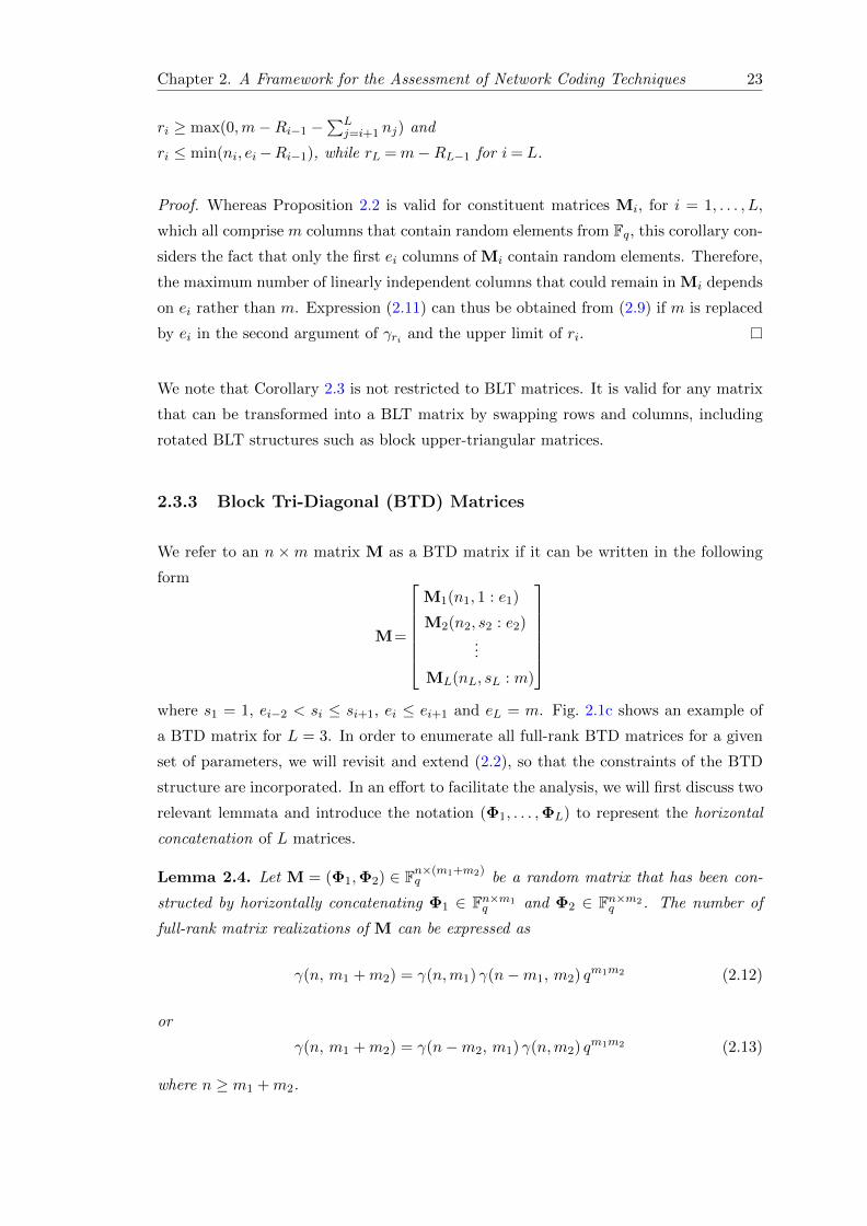
Chapter 2. A Framework for the Assessment of Network Coding Techniques 23
ri ≥ max(0,m−Ri−1 −∑L
j=i+1 nj) and
ri ≤ min(ni, ei−Ri−1), while rL =m−RL−1 for i= L.
Proof. Whereas Proposition 2.2 is valid for constituent matrices Mi, for i = 1, . . . , L,
which all comprise m columns that contain random elements from Fq, this corollary con-
siders the fact that only the first ei columns of Mi contain random elements. Therefore,
the maximum number of linearly independent columns that could remain in Mi depends
on ei rather than m. Expression (2.11) can thus be obtained from (2.9) if m is replaced
by ei in the second argument of γri and the upper limit of ri.
We note that Corollary 2.3 is not restricted to BLT matrices. It is valid for any matrix
that can be transformed into a BLT matrix by swapping rows and columns, including
rotated BLT structures such as block upper-triangular matrices.
2.3.3 Block Tri-Diagonal (BTD) Matrices
We refer to an n ×m matrix M as a BTD matrix if it can be written in the following
form
M=
M1(n1, 1 : e1)
M2(n2, s2 : e2)...
ML(nL, sL : m)
where s1 = 1, ei−2 < si ≤ si+1, ei ≤ ei+1 and eL = m. Fig. 2.1c shows an example of
a BTD matrix for L = 3. In order to enumerate all full-rank BTD matrices for a given
set of parameters, we will revisit and extend (2.2), so that the constraints of the BTD
structure are incorporated. In an effort to facilitate the analysis, we will first discuss two
relevant lemmata and introduce the notation (Φ1, . . . ,ΦL) to represent the horizontal
concatenation of L matrices.
Lemma 2.4. Let M = (Φ1,Φ2) ∈ Fn×(m1+m2)q be a random matrix that has been con-
structed by horizontally concatenating Φ1 ∈ Fn×m1q and Φ2 ∈ Fn×m2
q . The number of
full-rank matrix realizations of M can be expressed as
γ(n, m1 +m2) = γ(n,m1) γ(n−m1, m2) qm1m2 (2.12)
or
γ(n, m1 +m2) = γ(n−m2, m1) γ(n,m2) qm1m2 (2.13)
where n ≥ m1 +m2.
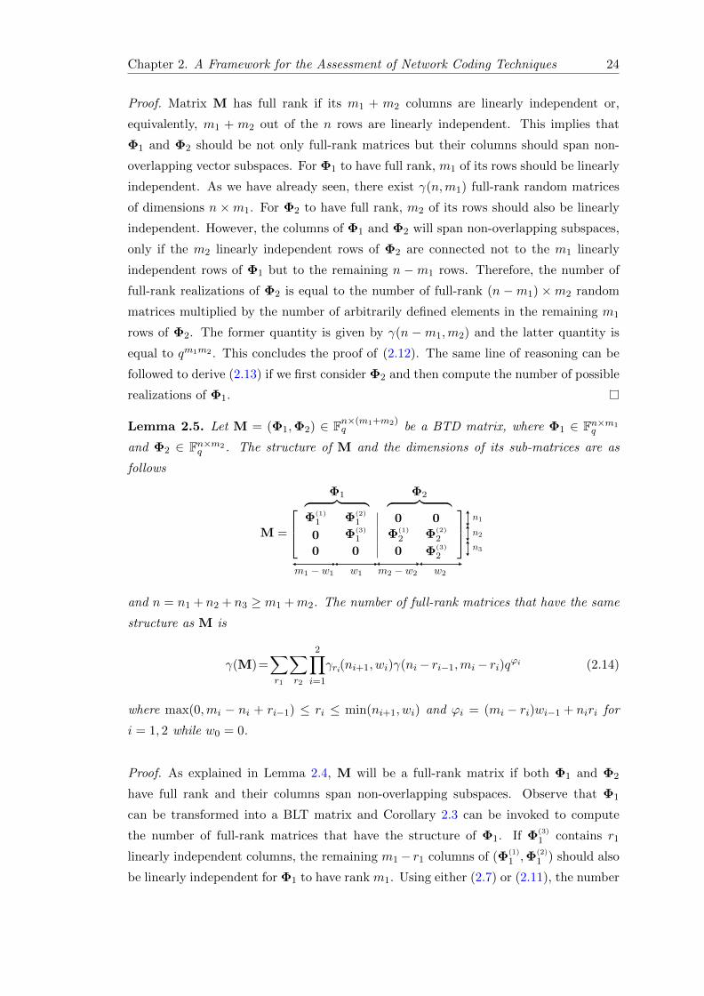
Chapter 2. A Framework for the Assessment of Network Coding Techniques 24
Proof. Matrix M has full rank if its m1 + m2 columns are linearly independent or,
equivalently, m1 + m2 out of the n rows are linearly independent. This implies that
Φ1 and Φ2 should be not only full-rank matrices but their columns should span non-
overlapping vector subspaces. For Φ1 to have full rank, m1 of its rows should be linearly
independent. As we have already seen, there exist γ(n,m1) full-rank random matrices
of dimensions n ×m1. For Φ2 to have full rank, m2 of its rows should also be linearly
independent. However, the columns of Φ1 and Φ2 will span non-overlapping subspaces,
only if the m2 linearly independent rows of Φ2 are connected not to the m1 linearly
independent rows of Φ1 but to the remaining n −m1 rows. Therefore, the number of
full-rank realizations of Φ2 is equal to the number of full-rank (n −m1) ×m2 random
matrices multiplied by the number of arbitrarily defined elements in the remaining m1
rows of Φ2. The former quantity is given by γ(n −m1,m2) and the latter quantity is
equal to qm1m2 . This concludes the proof of (2.12). The same line of reasoning can be
followed to derive (2.13) if we first consider Φ2 and then compute the number of possible
realizations of Φ1.
Lemma 2.5. Let M = (Φ1,Φ2) ∈ Fn×(m1+m2)q be a BTD matrix, where Φ1 ∈ Fn×m1
q
and Φ2 ∈ Fn×m2q . The structure of M and the dimensions of its sub-matrices are as
follows
and n = n1 + n2 + n3 ≥ m1 +m2. The number of full-rank matrices that have the same
structure as M is
γ(M)=∑r1
∑r2
2∏i=1
γri(ni+1, wi)γ(ni− ri−1,mi− ri)qϕi (2.14)
where max(0,mi − ni + ri−1) ≤ ri ≤ min(ni+1, wi) and ϕi = (mi − ri)wi−1 + niri for
i = 1, 2 while w0 = 0.
Proof. As explained in Lemma 2.4, M will be a full-rank matrix if both Φ1 and Φ2
have full rank and their columns span non-overlapping subspaces. Observe that Φ1
can be transformed into a BLT matrix and Corollary 2.3 can be invoked to compute
the number of full-rank matrices that have the structure of Φ1. If Φ(3)
1 contains r1
linearly independent columns, the remaining m1− r1 columns of (Φ(1)
1 ,Φ(2)
1 ) should also
be linearly independent for Φ1 to have rank m1. Using either (2.7) or (2.11), the number
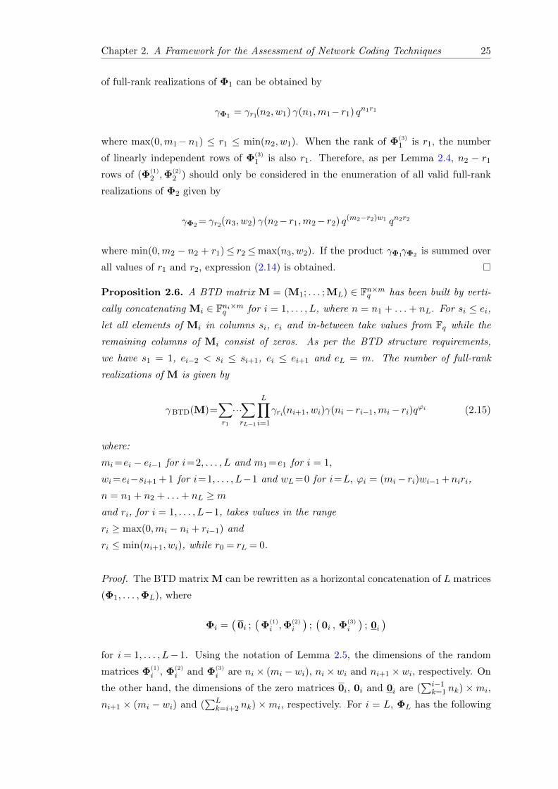
Chapter 2. A Framework for the Assessment of Network Coding Techniques 25
of full-rank realizations of Φ1 can be obtained by
γΦ1 = γr1(n2, w1) γ(n1,m1− r1) qn1r1
where max(0,m1− n1) ≤ r1 ≤ min(n2, w1). When the rank of Φ(3)
1 is r1, the number
of linearly independent rows of Φ(3)
1 is also r1. Therefore, as per Lemma 2.4, n2 − r1
rows of (Φ(1)
2 ,Φ(2)
2 ) should only be considered in the enumeration of all valid full-rank
realizations of Φ2 given by
γΦ2 = γr2(n3, w2) γ(n2− r1,m2− r2) q(m2−r2)w1 qn2r2
where min(0,m2 − n2 + r1)≤ r2 ≤max(n3, w2). If the product γΦ1γΦ2 is summed over
all values of r1 and r2, expression (2.14) is obtained.
Proposition 2.6. A BTD matrix M = (M1; . . . ; ML) ∈ Fn×mq has been built by verti-
cally concatenating Mi ∈ Fni×mq for i = 1, . . . , L, where n = n1 + . . .+ nL. For si ≤ ei,let all elements of Mi in columns si, ei and in-between take values from Fq while the
remaining columns of Mi consist of zeros. As per the BTD structure requirements,
we have s1 = 1, ei−2 < si ≤ si+1, ei ≤ ei+1 and eL = m. The number of full-rank
realizations of M is given by
γBTD(M)=∑r1
···∑rL−1
L∏i=1
γri(ni+1, wi)γ(ni− ri−1,mi− ri)qϕi (2.15)
where:
mi=ei − ei−1 for i=2, . . . , L and m1 =e1 for i = 1,
wi=ei−si+1 + 1 for i=1, . . . , L−1 and wL=0 for i=L, ϕi = (mi− ri)wi−1 +niri,
n = n1 + n2 + . . .+ nL ≥ mand ri, for i = 1, . . . , L−1, takes values in the range
ri ≥ max(0,mi − ni + ri−1) and
ri ≤ min(ni+1, wi), while r0 = rL = 0.
Proof. The BTD matrix M can be rewritten as a horizontal concatenation of L matrices
(Φ1, . . . ,ΦL), where
Φi =(0i ;
(Φ(1)
i ,Φ(2)
i
);(0i , Φ(3)
i
); 0i
)for i = 1, . . . , L− 1. Using the notation of Lemma 2.5, the dimensions of the random
matrices Φ(1)
i , Φ(2)
i and Φ(3)
i are ni × (mi −wi), ni ×wi and ni+1 ×wi, respectively. On
the other hand, the dimensions of the zero matrices 0i, 0i and 0i are (∑i−1
k=1 nk) ×mi,
ni+1 × (mi − wi) and (∑L
k=i+2 nk) ×mi, respectively. For i = L, ΦL has the following
Chapter 2. A Framework for the Assessment of Network Coding Techniques 26
structure
ΦL =(0L ; Φ(1)
L
)where 0L is the (n − nL) × mL zero matrix and Φ(1)
L is an nL × mL random matrix.
If we consider the first L− 1 sub-matrices only, the number of full-rank matrices with
structure (Φ1, . . . ,ΦL−1) is
γ (Φ1,...,ΦL−1)=∑r1
···∑rL−1
L−1∏i=1
γri(ni+1, wi)γ(ni− ri−1,mi− ri)qϕi (2.16)
as per Lemma 2.5. The inclusion of the last sub-matrix ΦL will increase the number of
full-rank realisations of M by a factor of γΦL , where
γΦL = γ(nL− rL−1, mL) qmLwL−1 . (2.17)
The product of (2.16) and (2.17) gives (2.15). Notice that (2.17) can be incorporated
into (2.16) if we change the upper limit of the summation index i from L− 1 to L and
set rL = 0.
This section focused on random block matrices and demonstrated that Proposition 2.2
can be used to compute the number of full-rank BD matrices but, as Corollary 2.3
explained, it can also be extended to the case of BLT matrices. Proposition 2.6 was
introduced for the enumeration of full-rank BTD matrices. The following section will
discuss how the analysis of random block matrices can be used in the performance
assessment of practical network coding techniques.
2.4 Assessment of Network Coding Techniques
In conventional network coding (NC), a source node segments a message into m source
packets of equal length, linearly combines them over the finite field Fq and generates
n coded packets. This implies that the ith coded packet yi, for i = 1, . . . , n, can be
expressed as follows
yi =m∑j=1
ci,jxj (2.18)
where xj represents the jth source packet of the message. As already described in Chap-
ter 1, that the coefficients ci,j are selected uniformly at random over the finite field Fq in
RLNC. For a given value of i, the sequence ci,1, ci,2, . . . , ci,m forms a row vector, which
is known as the coding vector of the output coded packet yi, and is transmitted along
with yi in the packet header. Using matrix notation, expression (2.18) can be rewritten
Chapter 2. A Framework for the Assessment of Network Coding Techniques 27
as
Y = CX (2.19)
where Y ∈ Fn×1q , C ∈ Fn×mq and X ∈ Fm×1
q are the matrices whose elements are yi, ci,j
and xj , respectively. Matrix C is also known as the coding matrix.
At a receiving node, when n ≥ m coded packets have been received, the coding vectors
of the received coded packets are stacked together to generate a decoding matrix D of
dimensions n×m. A receiver can successfully decode the source message if and only if
m linearly independent coded packets have been received or, equivalently, the rank of
D is m. Therefore, the probability of successful decoding a source message, given that
n coded packets have been received, is associated with the full-rank probability of D,
which is given by P (n,m) in (2.2).
If the transmission of the n ≥ n coded packets is modeled as a sequence of n Bernoulli
trials, whereby ε signifies the probability that a transmitted coded packet will be erased,
the probability of a receiving node decoding the source message for a coding matrix C
and all possible realizations of the decoding matrix D can be written as
Pdec(C) =
n∑n=m
B(n, n, ε)P (n,m) (2.20)
where B(n, n, ε) is the probability mass function of the binomial distribution, given by
B(n, n, ε) =
(n
n
)(1− ε)n εn−n. (2.21)
Due to the fact that both the coding matrix C and the decoding matrix D can be
very dense, RLNC is referred to as a dense code [104] and the decoding process can
be computationally expensive. Various layered RLNC schemes have been considered in
the literature as a means to reduce the complexity of conventional RLNC or introduce
unequal error protection. These schemes organize the m source packets into L over-
lapping or non-overlapping groups, referred to as generations [105]. The remainder of
this section is concerned with the characterization of the decoding probability of three
widely-used layered RLNC schemes using expressions (2.10), (2.11) and (2.15).
2.4.1 Non-Overlapping Generations RLNC (NOG-RLNC)
Let the ith generation, denoted by Gi, contain ki source packets. When each packet be-
longs to a single generation only, the generations are non-overlapping, i.e., Gi ∩Gj = ∅for all i 6= j, as shown in Fig. 2.2. Similarly, if mi denotes the number of source packets
in Gi that are not shared with any other generation, we can write mi = ki for any
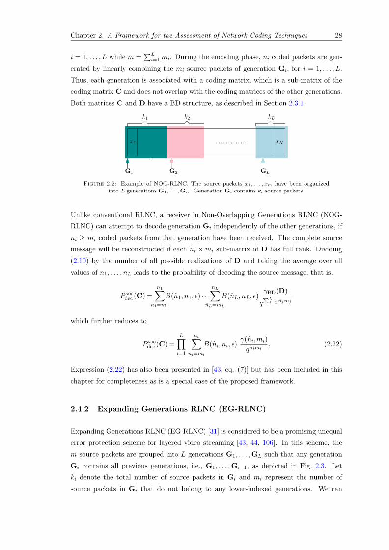
Chapter 2. A Framework for the Assessment of Network Coding Techniques 28
i = 1, . . . , L while m =∑L
i=1mi. During the encoding phase, ni coded packets are gen-
erated by linearly combining the mi source packets of generation Gi, for i = 1, . . . , L.
Thus, each generation is associated with a coding matrix, which is a sub-matrix of the
coding matrix C and does not overlap with the coding matrices of the other generations.
Both matrices C and D have a BD structure, as described in Section 2.3.1.
k2k1 kL
x1 xK
G1 G2 GL
Figure 2.2: Example of NOG-RLNC. The source packets x1, . . . , xm have been organizedinto L generations G1, . . . ,GL. Generation Gi contains ki source packets.
Unlike conventional RLNC, a receiver in Non-Overlapping Generations RLNC (NOG-
RLNC) can attempt to decode generation Gi independently of the other generations, if
ni ≥ mi coded packets from that generation have been received. The complete source
message will be reconstructed if each ni ×mi sub-matrix of D has full rank. Dividing
(2.10) by the number of all possible realizations of D and taking the average over all
values of n1, . . . , nL leads to the probability of decoding the source message, that is,
P NOG
dec (C) =
n1∑n1=m1
B(n1, n1, ε) · · ·nL∑
nL=mL
B(nL, nL, ε)γBD(D)
q∑Lj=1 njmj
which further reduces to
P NOG
dec (C) =L∏i=1
ni∑ni=mi
B(ni, ni, ε)γ(ni,mi)
qnimi. (2.22)
Expression (2.22) has also been presented in [43, eq. (7)] but has been included in this
chapter for completeness as is a special case of the proposed framework.
2.4.2 Expanding Generations RLNC (EG-RLNC)
Expanding Generations RLNC (EG-RLNC) [31] is considered to be a promising unequal
error protection scheme for layered video streaming [43, 44, 106]. In this scheme, the
m source packets are grouped into L generations G1, . . . ,GL such that any generation
Gi contains all previous generations, i.e., G1, . . . ,Gi−1, as depicted in Fig. 2.3. Let
ki denote the total number of source packets in Gi and mi represent the number of
source packets in Gi that do not belong to any lower-indexed generations. We can
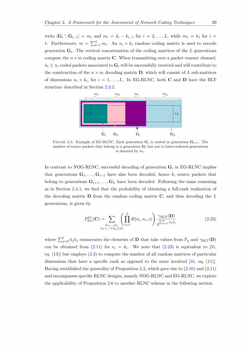
Chapter 2. A Framework for the Assessment of Network Coding Techniques 29
write |Gi \ Gi−1| = mi and mi = ki − ki−1 for i = 2, . . . , L, while m1 = k1 for i =
1. Furthermore, m =∑L
i=1mi. An ni × ki random coding matrix is used to encode
generation Gi. The vertical concatenation of the coding matrices of the L generations
compose the n×m coding matrix C. When transmitting over a packet erasure channel,
ni ≤ ni coded packets associated to Gi will be successfully received and will contribute to
the construction of the n×m decoding matrix D, which will consist of L sub-matrices
of dimensions ni × ki, for i = 1, . . . , L. In EG-RLNC, both C and D have the BLT
structure described in Section 2.3.2.
G1 G2 Gi GL
m1 m2 mi mL
x1 xK
Figure 2.3: Example of EG-RLNC. Each generation Gi is nested in generation Gi+1. Thenumber of source packets that belong to a generation Gi but not to lower-indexed generations
is denoted by mi.
In contrast to NOG-RLNC, successful decoding of generation Gi in EG-RLNC implies
that generations G1, . . . ,Gi−1 have also been decoded, hence ki source packets that
belong to generations Gi+1, . . . ,GL have been decoded. Following the same reasoning
as in Section 2.4.1, we find that the probability of obtaining a full-rank realization of
the decoding matrix D from the random coding matrix C, and thus decoding the L
generations, is given by
P EGdec(C) =
∑n1,...,nL
n1+...+nL≥m
(L∏i=1
B(ni, ni, ε)
)γBLT(D)
q∑Lj=1 njkj
(2.23)
where∑`
j=0 njkj enumerates the elements of D that take values from Fq and γBLT(D)
can be obtained from (2.11) for ei = ki. We note that (2.23) is equivalent to [31,
eq. (13)] but employs (2.3) to compute the number of all random matrices of particular
dimensions that have a specific rank as opposed to the more involved [31, eq. (11)].
Having established the generality of Proposition 2.2, which gave rise to (2.10) and (2.11)
and encompasses specific RLNC designs, namely NOG-RLNC and EG-RLNC, we explore
the applicability of Proposition 2.6 to another RLNC scheme in the following section.
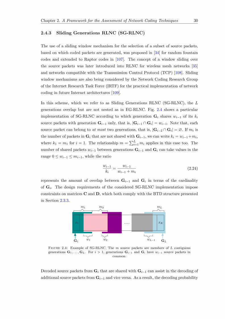
Chapter 2. A Framework for the Assessment of Network Coding Techniques 30
2.4.3 Sliding Generations RLNC (SG-RLNC)
The use of a sliding window mechanism for the selection of a subset of source packets,
based on which coded packets are generated, was proposed in [34] for random fountain
codes and extended to Raptor codes in [107]. The concept of a window sliding over
the source packets was later introduced into RLNC for wireless mesh networks [35]
and networks compatible with the Transmission Control Protocol (TCP) [108]. Sliding
window mechanisms are also being considered by the Network Coding Research Group
of the Internet Research Task Force (IRTF) for the practical implementation of network
coding in future Internet architectures [109].
In this scheme, which we refer to as Sliding Generations RLNC (SG-RLNC), the L
generations overlap but are not nested as in EG-RLNC. Fig. 2.4 shows a particular
implementation of SG-RLNC according to which generation Gi shares wi−1 of its ki
source packets with generation Gi−1 only, that is, |Gi−1 ∩Gi| = wi−1. Note that, each
source packet can belong to at most two generations, that is, |Gi−2 ∩Gi| = ∅. If mi is
the number of packets in Gi that are not shared with Gi−1, we can write ki = wi−1 +mi,
where k1 = m1 for i = 1. The relationship m =∑L
i=1mi applies in this case too. The
number of shared packets wi−1 between generations Gi−1 and Gi can take values in the
range 0 ≤ wi−1 ≤ mi−1, while the ratio
wi−1
ki=
wi−1
wi−1 +mi(2.24)
represents the amount of overlap between Gi−1 and Gi in terms of the cardinality
of Gi. The design requirements of the considered SG-RLNC implementation impose
constraints on matrices C and D, which both comply with the BTD structure presented
in Section 2.3.3.
G1 GLw1 w2 wL−1
x1 xK
m1 m2 mL
Figure 2.4: Example of SG-RLNC. The m source packets are members of L contiguousgenerations G1, . . . ,GL. For i > 1, generations Gi−1 and Gi have wi−1 source packets in
common.
Decoded source packets from Gi that are shared with Gi−1 can assist in the decoding of
additional source packets from Gi−1 and vice versa. As a result, the decoding probability
Chapter 2. A Framework for the Assessment of Network Coding Techniques 31
of each generation will be higher than that of NOG-RLNC but lower than that of EG-
RLNC. If the coding matrix C dictates the transmission of ni coded packets associated
with generation Gi over a packet erasure channel and ni of them are received, the
probability that the decoding matrix D will have full rank assumes a similar expression
to (2.23), i.e.,
P SGdec(C) =
∑n1,...,nL
n1+...+nL≥m
(L∏i=1
B(ni, ni, ε)
)γBTD(D)
q∑Lj=1 njkj
(2.25)
where γBTD(D) can be obtained from (2.15) for mi = ki − wi−1 when i = 2, . . . , L and
m1 = k1 for i = 1.
It is important to emphasize that the requirement for wi ≤ mi in the considered SG-
RLNC scheme stems from the constraint ei−2 ≤ si+1 in Proposition 2.6, which implies
that the overlap between two adjacent generations in the SG-RLNC implementation
shown in Fig. 2.4 cannot exceed 50%, which is achieved for wi−1 = mi based on (2.24).
Although each source packet could belong to more than two generations in the general
case of SG-RLNC, Section 2.5 will demonstrate that an overlap smaller than 50% suf-
fices for SG-RLNC to yield the same decoding probability as EG-RLNC for low erasure
probabilities. Considering that RLNC is an Application Layer Forward Error Correc-
tion (AL-FEC) scheme, typical values of the erasure probability are ε ≤ 0.2 for TCP
traffic [108] and ε ≤ 0.1 for Long Term Evolution (LTE) systems [110]. We can thus
conclude that Proposition 2.6 can be used to characterize the decoding probability of a
constrained, yet practical, class of SG-RLNC implementations.
2.5 Results and Discussions
The previous sections developed a mathematical framework for enumerating particular
structures of full-rank random block matrices, which formed the basis for the perfor-
mance evaluation of well-known RLNC schemes that use the concepts of non-overlapping,
expanding and sliding generations. This section is concerned with the validation of the
derived theoretical expressions and the performance comparison of the three considered
RNLC schemes.
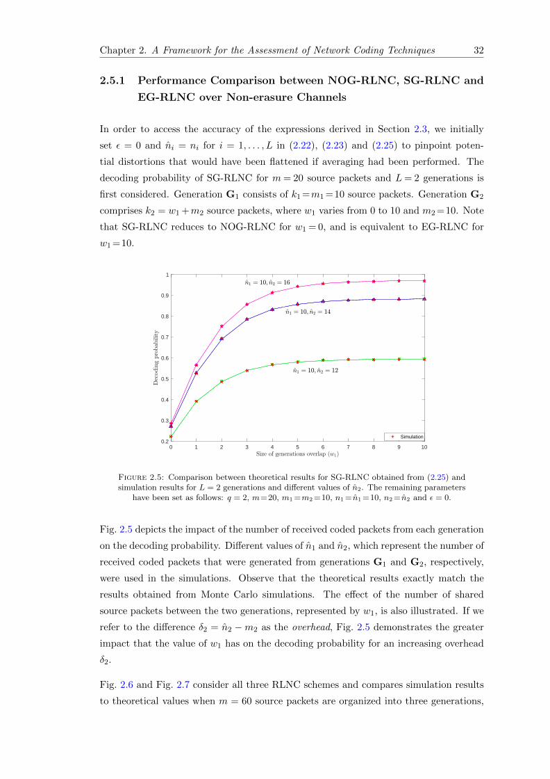
Chapter 2. A Framework for the Assessment of Network Coding Techniques 32
2.5.1 Performance Comparison between NOG-RLNC, SG-RLNC and
EG-RLNC over Non-erasure Channels
In order to access the accuracy of the expressions derived in Section 2.3, we initially
set ε = 0 and ni = ni for i = 1, . . . , L in (2.22), (2.23) and (2.25) to pinpoint poten-
tial distortions that would have been flattened if averaging had been performed. The
decoding probability of SG-RLNC for m= 20 source packets and L= 2 generations is
first considered. Generation G1 consists of k1 =m1 =10 source packets. Generation G2
comprises k2 = w1 +m2 source packets, where w1 varies from 0 to 10 and m2 =10. Note
that SG-RLNC reduces to NOG-RLNC for w1 = 0, and is equivalent to EG-RLNC for
w1 =10.
0 1 2 3 4 5 6 7 8 9 100.2
0.3
0.4
0.5
0.6
0.7
0.8
0.9
1
Simulation
Figure 2.5: Comparison between theoretical results for SG-RLNC obtained from (2.25) andsimulation results for L = 2 generations and different values of n2. The remaining parameters
have been set as follows: q = 2, m=20, m1 =m2 =10, n1 = n1 =10, n2 = n2 and ε = 0.
Fig. 2.5 depicts the impact of the number of received coded packets from each generation
on the decoding probability. Different values of n1 and n2, which represent the number of
received coded packets that were generated from generations G1 and G2, respectively,
were used in the simulations. Observe that the theoretical results exactly match the
results obtained from Monte Carlo simulations. The effect of the number of shared
source packets between the two generations, represented by w1, is also illustrated. If we
refer to the difference δ2 = n2 −m2 as the overhead, Fig. 2.5 demonstrates the greater
impact that the value of w1 has on the decoding probability for an increasing overhead
δ2.
Fig. 2.6 and Fig. 2.7 consider all three RLNC schemes and compares simulation results
to theoretical values when m = 60 source packets are organized into three generations,
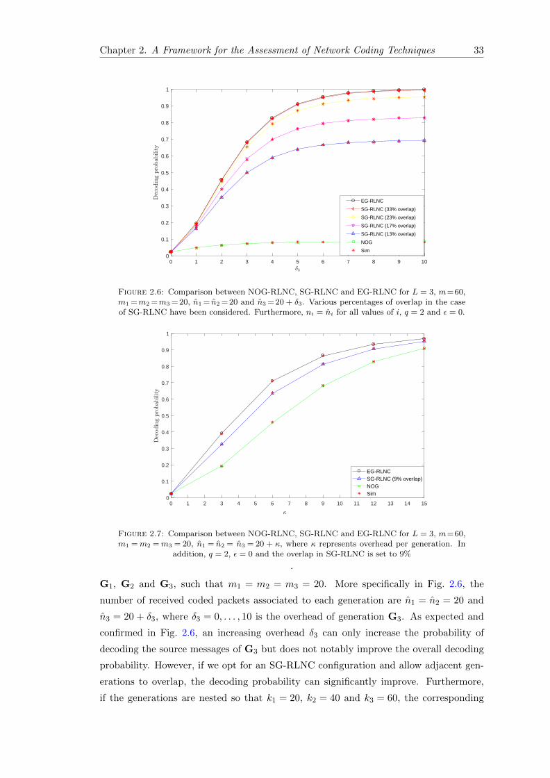
Chapter 2. A Framework for the Assessment of Network Coding Techniques 33
0 1 2 3 4 5 6 7 8 9 100
0.1
0.2
0.3
0.4
0.5
0.6
0.7
0.8
0.9
1
EG-RLNC
SG-RLNC (33% overlap)
SG-RLNC (23% overlap)
SG-RLNC (17% overlap)
SG-RLNC (13% overlap)
NOG
Sim
Figure 2.6: Comparison between NOG-RLNC, SG-RLNC and EG-RLNC for L = 3, m=60,m1 =m2 =m3 = 20, n1 = n2 = 20 and n3 = 20 + δ3. Various percentages of overlap in the caseof SG-RLNC have been considered. Furthermore, ni = ni for all values of i, q = 2 and ε = 0.
0 1 2 3 4 5 6 7 8 9 10 11 12 13 14 150
0.1
0.2
0.3
0.4
0.5
0.6
0.7
0.8
0.9
1
EG-RLNCSG-RLNC (9% overlap)NOGSim
Figure 2.7: Comparison between NOG-RLNC, SG-RLNC and EG-RLNC for L = 3, m=60,m1 =m2 =m3 = 20, n1 = n2 = n3 = 20 + κ, where κ represents overhead per generation. In
addition, q = 2, ε = 0 and the overlap in SG-RLNC is set to 9%
.
G1, G2 and G3, such that m1 = m2 = m3 = 20. More specifically in Fig. 2.6, the
number of received coded packets associated to each generation are n1 = n2 = 20 and
n3 = 20 + δ3, where δ3 = 0, . . . , 10 is the overhead of generation G3. As expected and
confirmed in Fig. 2.6, an increasing overhead δ3 can only increase the probability of
decoding the source messages of G3 but does not notably improve the overall decoding
probability. However, if we opt for an SG-RLNC configuration and allow adjacent gen-
erations to overlap, the decoding probability can significantly improve. Furthermore,
if the generations are nested so that k1 = 20, k2 = 40 and k3 = 60, the corresponding
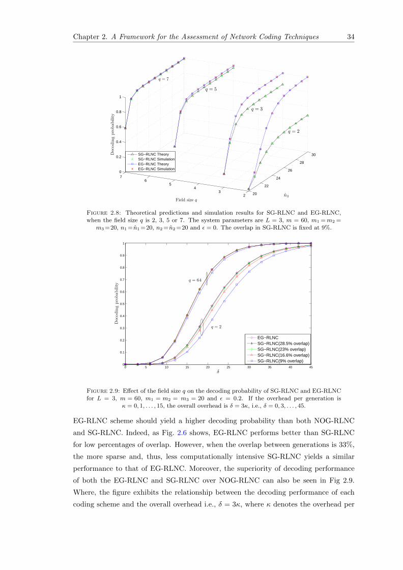
Chapter 2. A Framework for the Assessment of Network Coding Techniques 34
20
22
24
26
28
30
23
45
670
0.2
0.4
0.6
0.8
1
n3Field size q
Decodingprobability
SG−RLNC TheorySG−RLNC SimulationEG−RLNC TheoryEG−RLNC Simulation
q = 7
q = 5
q = 3
q = 2
Figure 2.8: Theoretical predictions and simulation results for SG-RLNC and EG-RLNC,when the field size q is 2, 3, 5 or 7. The system parameters are L = 3, m = 60, m1 =m2 =
m3 =20, n1 = n1 =20, n2 = n2 =20 and ε = 0. The overlap in SG-RLNC is fixed at 9%.
0 5 10 15 20 25 30 35 40 450
0.1
0.2
0.3
0.4
0.5
0.6
0.7
0.8
0.9
1
δ
Decodingprobability
EG−RLNCSG−RLNC(28.5% overlap)SG−RLNC(23% overlap)SG−RLNC(16.6% overlap)SG−RLNC(9% overlap)
q = 2
q = 64
Figure 2.9: Effect of the field size q on the decoding probability of SG-RLNC and EG-RLNCfor L = 3, m = 60, m1 = m2 = m3 = 20 and ε = 0.2. If the overhead per generation is
κ = 0, 1, . . . , 15, the overall overhead is δ = 3κ, i.e., δ = 0, 3, . . . , 45.
EG-RLNC scheme should yield a higher decoding probability than both NOG-RLNC
and SG-RLNC. Indeed, as Fig. 2.6 shows, EG-RLNC performs better than SG-RLNC
for low percentages of overlap. However, when the overlap between generations is 33%,
the more sparse and, thus, less computationally intensive SG-RLNC yields a similar
performance to that of EG-RLNC. Moreover, the superiority of decoding performance
of both the EG-RLNC and SG-RLNC over NOG-RLNC can also be seen in Fig 2.9.
Where, the figure exhibits the relationship between the decoding performance of each
coding scheme and the overall overhead i.e., δ = 3κ, where κ denotes the overhead per
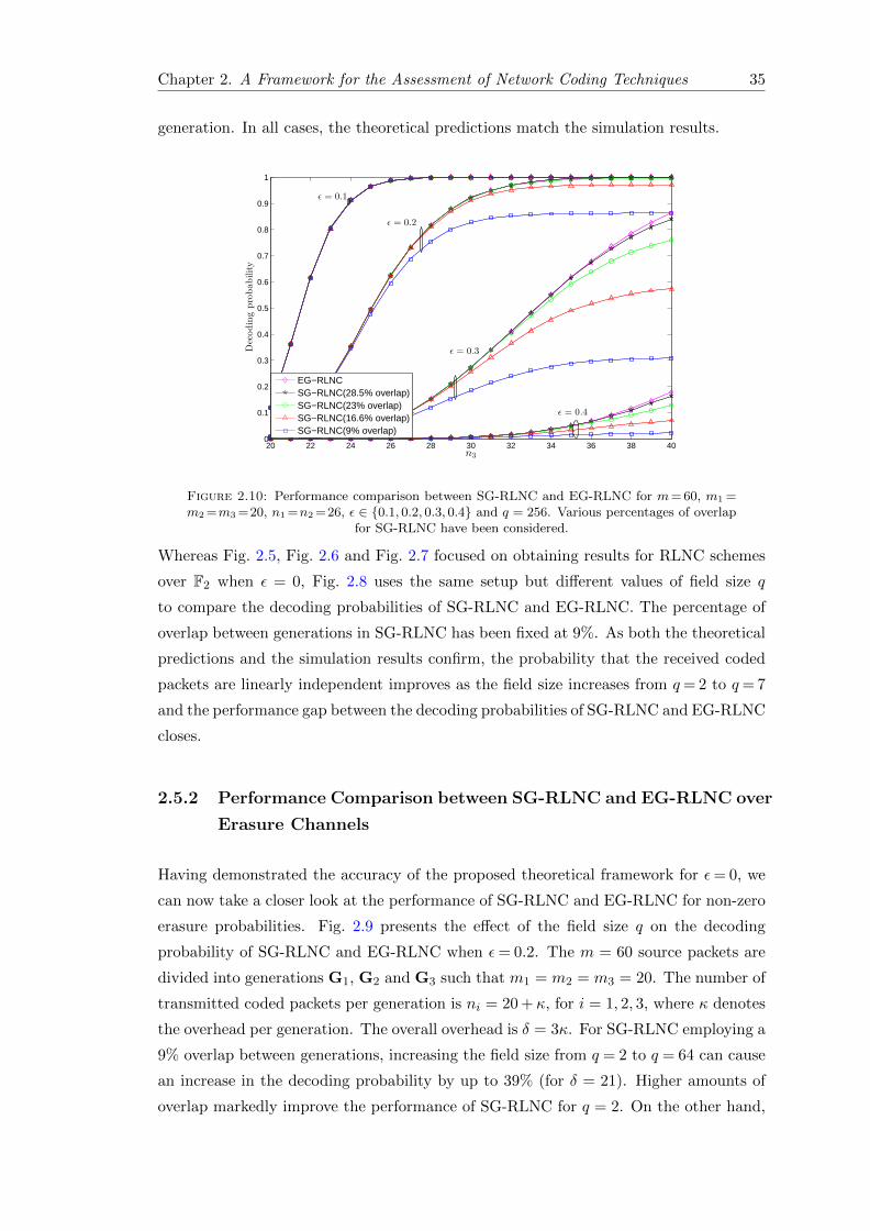
Chapter 2. A Framework for the Assessment of Network Coding Techniques 35
generation. In all cases, the theoretical predictions match the simulation results.
20 22 24 26 28 30 32 34 36 38 400
0.1
0.2
0.3
0.4
0.5
0.6
0.7
0.8
0.9
1
n3
Decodingprobability
EG−RLNCSG−RLNC(28.5% overlap)SG−RLNC(23% overlap)SG−RLNC(16.6% overlap)SG−RLNC(9% overlap)
ǫ = 0.1
ǫ = 0.2
ǫ = 0.3
ǫ = 0.4
Figure 2.10: Performance comparison between SG-RLNC and EG-RLNC for m= 60, m1 =m2 =m3 =20, n1 =n2 =26, ε ∈ {0.1, 0.2, 0.3, 0.4} and q = 256. Various percentages of overlap
for SG-RLNC have been considered.
Whereas Fig. 2.5, Fig. 2.6 and Fig. 2.7 focused on obtaining results for RLNC schemes
over F2 when ε = 0, Fig. 2.8 uses the same setup but different values of field size q
to compare the decoding probabilities of SG-RLNC and EG-RLNC. The percentage of
overlap between generations in SG-RLNC has been fixed at 9%. As both the theoretical
predictions and the simulation results confirm, the probability that the received coded
packets are linearly independent improves as the field size increases from q= 2 to q= 7
and the performance gap between the decoding probabilities of SG-RLNC and EG-RLNC
closes.
2.5.2 Performance Comparison between SG-RLNC and EG-RLNC over
Erasure Channels
Having demonstrated the accuracy of the proposed theoretical framework for ε= 0, we
can now take a closer look at the performance of SG-RLNC and EG-RLNC for non-zero
erasure probabilities. Fig. 2.9 presents the effect of the field size q on the decoding
probability of SG-RLNC and EG-RLNC when ε= 0.2. The m = 60 source packets are
divided into generations G1, G2 and G3 such that m1 = m2 = m3 = 20. The number of
transmitted coded packets per generation is ni = 20 + κ, for i = 1, 2, 3, where κ denotes
the overhead per generation. The overall overhead is δ = 3κ. For SG-RLNC employing a
9% overlap between generations, increasing the field size from q = 2 to q = 64 can cause
an increase in the decoding probability by up to 39% (for δ = 21). Higher amounts of
overlap markedly improve the performance of SG-RLNC for q = 2. On the other hand,
Chapter 2. A Framework for the Assessment of Network Coding Techniques 36
an increase in the overlap from 9% to 16.6% is sufficient for SG-RLNC to achieve a
performance comparable to that of EG-RLNC for q = 64.
Fig. 2.10 compares the performance of SG-RLNC and EG-RLNC for q = 256 in var-
ious channel conditions represented by different erasure probabilities. Both schemes
consider m = 60 source packets distributed among generations G1, G2 and G3, such
that m1 = m2 = m3 = 20. The number of transmitted coded packets per genetation
are n1 = n2 = 26 and n3 = 20, . . . , 40. Fig. 2.10 shows that, when large finite fields
are used, the decoding probabilities of the considered schemes are indistinguishable for
erasure probabilities as low as 0.1. As the channel conditions deteriorate, low percent-
ages of overlap can significantly degrade the performance of SG-RLNC. Nevertheless, a
28.5% overlap between generations is still sufficient for SG-RLNC to achieve a decoding
probability similar to that of EG-RLNC, even for ε = 0.4.
2.6 Summary
In this chapter, we focused on random block matrices and investigated three different
matrix structures over finite fields. In particular, we presented a framework based on
which exact analytical expressions were derived for the number of full-rank matrices
complying with each structure. Furthermore, we mapped the three matrix structures
onto RLNC schemes that are available in the literature and use the concepts of non-
overlapping, expanding and sliding generations to either reduce the decoding complexity
or incorporate unequal error protection features. The design parameters of these schemes
allow to adjust the level of sparsity and the desired decoding performance. We observed
the trade-off between the sparsity and the decoding performance, i.e., the higher the
sparsity is, the lower the decoding performance will be. More importantly, the derived
expressions for RLNC using sliding generations that can overlap by up to 50% demon-
strated that a low amount of overlap between generations in practical settings can yield
a similar decoding probability to that of the more computationally expensive RLNC
based on expanding generations. In this chapter, specifically, we made the following
contributions:
• We derived expressions for the enumeration of full-rank matrices that are con-
structed by the vertical (Lemma 2.1) or horizontal (Lemmata 2.4 and 2.5) con-
catenation of random matrices or random block matrices over finite fields.
• We revisited the formula that computes the number of full-rank random matri-
ces and rewrote it for the case of partitioned random matrices (Proposition 2.2).
Chapter 2. A Framework for the Assessment of Network Coding Techniques 37
We then extended this formula to random block lower-triangular matrices (Corol-
lary 2.3) and adjusted it for random block tri-diagonal matrices (Proposition 2.6).
• We demonstrated that the proposed framework offers a unified RMT-based ap-
proach for the analysis of practical RLNC schemes, which are described by ran-
dom block matrices over finite fields of any size. In particular, we showed that
our framework generates the well-known decoding probability of RLNC over non-
overlapping windows and a more compact expression for the decoding probability
of RLNC over expanding windows [31]. The proposed framework can also be used
for the performance analysis of RLNC over sliding windows, which is often carried
out based on simulations, e.g., [34].
Chapter 3
Random Linear Network Coding
for Coded Cooperation
In the previous chapter, we developed a mathematical framework to evaluate and charac-
terize the performance in terms of the decoding probability of RLNC techniques suitable
for broadcast or multicast communication. In this chapter, we aim to study and evaluate
the performance of RLNC in single-relay as well as multi-relay assisted cooperative net-
works. Finally, we propose and develop a novel framework which integrates the benefits
of NOMA and RLNC based cooperative relaying.
Section 3.1 of this chapter focuses on a network configuration that encompasses both
intra-session network coding at the source nodes, as in [111–113], and inter-session net-
work coding at the relay node, as in [7, 114, 115]. In our study, we have looked at the
decode-and-forward relaying scheme, that is, network-coded packets received by the re-
lay node are decoded and re-encoded before they are forwarded to the destination node.
The probability that the destination node will successfully decode the source packets
of both source nodes is used as the performance measure of the system. The derived
probability expressions could be adapted to other network-coded relaying strategies that
incorporate both intra-session and inter-session network coding schemes, as in [116], or
be used as benchmarks in performance comparisons.
Section 3.2 presents linear network coding over a multi-source multi-relay network, where
m source nodes are supported by n relay nodes for the delivery of packets over packet
erasure channels. To the best of our knowledge, an exact expression for the decoding
failure probability that the destination will fail to decode the packets of all source nodes
is not available but an effort has been made in [59], in which the author derives upper
and lower bounds. However, the bounds presented in [59] are tight only for a certain
range of parameters, including erasure probabilities, the values of m, n and the size
38
Chapter 3. Network Coded Cooperation 39
of the finite field. As shown in Section 3.2.4, the existing upper bound is poor for a
large number of source nodes and for large finite fields. Moreover, the existing lower
bound is independent of the field size and is loose for small finite fields and low erasure
probabilities. In this chapter our goal is to derive improved bounds on the probability
of decoding failure and demonstrate the performance.
As identified in Chapter 1, RLNC has also the potential to address ever increasing
number of users and devices in future cellular networks (5G and beyond 5G), and NOMA
can efficiently utilize the bandwidth resources. After the performance characterisation
of network coding based cooperation in Sections 3.1 and 3.2, Section 3.3 exploits the
network-coded cooperation in a NOMA-based scenario with two groups of source nodes,
where each group communicates with a different destination node via multiple relay
nodes. In this work, using the fundamentals of RLNC and uplink/downlink NOMA, we
derive closed-form expressions for the network performance, in terms of the decoding
probability at each node, and the system throughput. To the best of our knowledge,
this work represents the first attempt to characterise the performance of NOMA-based
RLNC cooperation.
3.1 Random Linear Network Coded Cooperation in Two
Source Single Relay Networks
This section considers the multiple-access relay channel in a setting where two source
nodes transmit packets to a destination node, both directly and via a relay node, over
packet erasure channels. Intra-session network coding is used at the source nodes and
inter-session network coding is employed at the relay node to combine the successfully
received source packets of both source nodes. In this work, we investigate the perfor-
mance of the network-coded system in terms of the probability that the destination
node will successfully decode the source packets of the two source nodes. We build our
analysis on fundamental probability expressions for random matrices over finite fields
and we derive upper bounds on the system performance for the case of systematic and
non-systematic network coding.
3.1.1 System Model and Problem Statement
We consider a network comprising two source nodes S1 and S2 having different data
contents, a relay node R and a destination node D, as shown in Fig. 3.1. Nodes S1 and S2
segment data into m1 and m2 equally-sized packets, respectively. Let x1, . . . , xm1 denote
the source packets of node S1 while xm1+1, . . . , xm1+m2 represent the source packets of
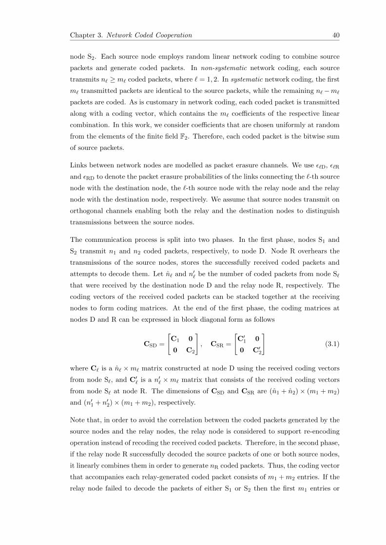
Chapter 3. Network Coded Cooperation 40
node S2. Each source node employs random linear network coding to combine source
packets and generate coded packets. In non-systematic network coding, each source
transmits n` ≥ m` coded packets, where ` = 1, 2. In systematic network coding, the first
m` transmitted packets are identical to the source packets, while the remaining n`−m`
packets are coded. As is customary in network coding, each coded packet is transmitted
along with a coding vector, which contains the m` coefficients of the respective linear
combination. In this work, we consider coefficients that are chosen uniformly at random
from the elements of the finite field F2. Therefore, each coded packet is the bitwise sum
of source packets.
Links between network nodes are modelled as packet erasure channels. We use ε`D, ε`R
and εRD to denote the packet erasure probabilities of the links connecting the `-th source
node with the destination node, the `-th source node with the relay node and the relay
node with the destination node, respectively. We assume that source nodes transmit on
orthogonal channels enabling both the relay and the destination nodes to distinguish
transmissions between the source nodes.
The communication process is split into two phases. In the first phase, nodes S1 and
S2 transmit n1 and n2 coded packets, respectively, to node D. Node R overhears the
transmissions of the source nodes, stores the successfully received coded packets and
attempts to decode them. Let n` and n′` be the number of coded packets from node S`
that were received by the destination node D and the relay node R, respectively. The
coding vectors of the received coded packets can be stacked together at the receiving
nodes to form coding matrices. At the end of the first phase, the coding matrices at
nodes D and R can be expressed in block diagonal form as follows
CSD =
[C1 0
0 C2
], CSR =
[C′1 0
0 C′2
](3.1)
where C` is a n` ×m` matrix constructed at node D using the received coding vectors
from node S`, and C′` is a n′` ×m` matrix that consists of the received coding vectors
from node S` at node R. The dimensions of CSD and CSR are (n1 + n2)× (m1 +m2)
and (n′1 + n′2)× (m1 +m2), respectively.
Note that, in order to avoid the correlation between the coded packets generated by the
source nodes and the relay nodes, the relay node is considered to support re-encoding
operation instead of recoding the received coded packets. Therefore, in the second phase,
if the relay node R successfully decoded the source packets of one or both source nodes,
it linearly combines them in order to generate nR coded packets. Thus, the coding vector
that accompanies each relay-generated coded packet consists of m1 +m2 entries. If the
relay node failed to decode the packets of either S1 or S2 then the first m1 entries or
Chapter 3. Network Coded Cooperation 41
D
S1
S2
R
ε1D
ε2D
εRD
ε1R
ε2R
n1
n2
nRnR
n′1
n′2
n2
n1
Figure 3.1: Block diagram of a network consisting of two source nodes S1 and S2, a relaynode R and a destination node D. The packet erasure probability of each link as well as the
number of transmitted and received coded packets at each node are also depicted.
the last m2 entries of the coding vector, respectively, are set to zero. If nR of the nR
transmitted coded packets are received by the destination node D, a nR × (m1 + m2)
coding matrix CRD will be created and appended to CSD. At the end of the second
phase, the coding matrix at node D is
CD =
[CSD
CRD
]=
C1 0
0 C2
CR1 CR2
(3.2)
which is a (n1 + n2 + nR)× (m1 +m2) block angular matrix. Note that CRD has been
expressed as the concatenation of matrices CR1 and CR2, which were generated by node
R and describe linear combinations of source packets originating from nodes S1 and S2,
respectively. Note that, all coded packets in the network have the same size, which is
customarily taken to be considerably larger than the size of the coding vectors.
The objective of this work is to characterise the system performance of the considered
two-source relay-aided network. More specifically, we will carry out a performance anal-
ysis to determine the probability that the destination node D will decode the m1 +m2
source packets of both nodes S1 and S2, given that node D has successfully received at
least m1 + m2 coded packets, that is, (n1 + n2 + nR) ≥ m1 + m2. The impact of the
chosen values for n and nR on the system performance will also be discussed.
Chapter 3. Network Coded Cooperation 42
3.1.2 Performance Analysis
Fundamental probabilities related to the rank of random matrices in F2 are summarised
in this section and are subsequently used in the derivation of expressions for the prob-
ability that the destination node D will successfully decode the source packets of both
source nodes, when they employ either non-systematic or systematic random linear net-
work coding.
3.1.2.1 Preliminaries: fundamental probability expressions
Let M be a n ×m binary random matrix with n ≥ m. As discussed in Chapter 2, we
say that M is a full-rank matrix if the rank of M is m or, equivalently, m of the n rows
of M are linearly independent. The probability of M being a full-rank matrix can be
obtained using (2.1) and (2.2) for F2, as follows
P (n,m) =γ(n,m)
2nm(3.3)
where 2nm is the number of all n×m binary matrices and γ(n,m) is the number of all
full-rank n×m binary matrices, given as
γ(n,m) =m−1∏i=0
(2n − 2i).
Similarly, the probability of M having rank r ≤ m when n ≥ r can be obtained by
employing (2.6) for F2, as follows
Pr(n,m) = 2−nm(γ(n, r)γ(m, r)
γ(r, r)
). (3.4)
Let us now assume that matrix M has the following constrained structure
M =
A 0
0 B
C D
(3.5)
where the dimensions of submatrices A, B, C and D are a× a′, b× b′, c× a′ and c× b′,respectively. Matrices of this type, which are known as block angular matrices, were
studied in [117]. It was proven that the probability of M being full-rank is given by
P (a, a′, b, b′, c)=∑
i+j≥a′+b′−cPi(a, a
′)Pj(b, b′)P (c, a′ + b′ − i− j). (3.6)
Chapter 3. Network Coded Cooperation 43
As implied by (3.6), the rank of matrix M is a′+b′ if submatrix A has rank i, submatrix
B has rank j and the remaining a′ + b′ − i− j columns of M are linearly independent,
for all valid values of i and j.
Expressions (3.3), (3.4) and (3.6) will be invoked in the subsequent performance analysis.
Note that character P is used exclusively to denote probabilities associated with the rank
of matrices but character P is used to refer to probabilities related to the system model
under consideration.
3.1.2.2 Decoding probability for non-systematic network coding
In the general case of point-to-point communication over a channel with erasure proba-
bility ε, the probability of the receiving node decoding all of the m source packets when
n coded packets have been transmitted can be obtained using (2.20), re-expressed as
follows
P(n,m, ε) =
n∑n=m
B(n, n, ε) P (n,m). (3.7)
Where, B(n, n, p) denotes the probability mass function of the binomial distribution,
defined in (2.21). Expression (3.7) enumerates all possible scenarios of retrieving the
m source packets when n ≥ m coded packets have been successfully received and have
formed a full-rank n×m coding matrix.
In the particular case of the considered relay-aided network, the probability that the des-
tination node D will decode the source packets of both source nodes can be decomposed
into the following three components:
Unaided communication: Even though the relay node R has been deployed in the
network, the destination node D could decode all of the source packets without the help
of node R. The implies that both submatrices C1 and C2 in (3.1) are full-rank matrices
and, consequently, CSD is also a full-rank matrix. Therefore, the probability that node
D will decode the m1 +m2 source packets based solely on the n1 +n2 transmitted coded
packets can be obtained using (3.7) as follows
PS = P(n1,m1, ε1D) P(n2,m2, ε2D). (3.8)
Partially aided communication: In this mode, the destination node decodes the m`
source packets of node S` based on coded packets transmitted both via the relay node
and over the direct link between S` and D. The destination node retrieves the source
packets of the other source node, denoted by S¯ where ¯ = 1, 2 and ¯ 6= `, without the
assistance of the relay node. The probability that node D will decode the m1+m2 source
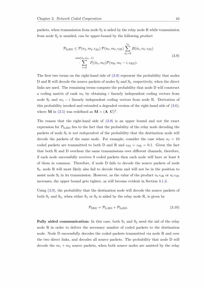
Chapter 3. Network Coded Cooperation 44
packets, when transmission from node S` is aided by the relay node R while transmission
from node S¯ is unaided, can be upper-bound by the following product
PS`RD ≤ P(n¯,m¯, ε¯D) P(n`,m`, ε`R)
n∑n`=0
B(n`, n`, ε`D)
·min(n`,m`−1)∑
i=0
Pi(n`,m`)P(nR,m` − i, εRD).
(3.9)
The first two terms on the right-hand side of (3.9) represent the probability that nodes
D and R will decode the source packets of nodes S¯ and S`, respectively, when the direct
links are used. The remaining terms compute the probability that node D will construct
a coding matrix of rank m` by obtaining i linearly independent coding vectors from
node S` and m` − i linearly independent coding vectors from node R. Derivation of
this probability invoked and extended a degraded version of the right-hand side of (3.6),
where M in (3.5) was redefined as M = (A C)ᵀ.
The reason that the right-hand side of (3.9) is an upper bound and not the exact
expression for PS`RD lies to the fact that the probability of the relay node decoding the
packets of node S` is not independent of the probability that the destination node will
decode the packets of the same node. For example, consider the case when n` = 10
coded packets are transmitted to both D and R and ε`D = ε`R = 0.1. Given the fact
that both R and D overhear the same transmissions over different channels, therefore,
if each node successfully receives 9 coded packets then each node will have at least 8
of them in common. Therefore, if node D fails to decode the source packets of node
S`, node R will most likely also fail to decode them and will not be in the position to
assist node S` in its transmission. However, as the value of the product n` ε`R or n` ε`D
increases, the upper bound gets tighter, as will become evident in Section 3.1.3.
Using (3.9), the probability that the destination node will decode the source packets of
both S1 and S2, when either S1 or S2 is aided by the relay node R, is given by
PSRD = PS1RD + PS2RD. (3.10)
Fully aided communication: In this case, both S1 and S2 need the aid of the relay
node R in order to deliver the necessary number of coded packets to the destination
node. Node D successfully decodes the coded packets transmitted via node R and over
the two direct links, and decodes all source packets. The probability that node D will
decode the m1 + m2 source packets, when both source nodes are assisted by the relay
Chapter 3. Network Coded Cooperation 45
node, can be upper-bound as follows
PRD ≤P(n1,m1, ε1R) P(n2,m2, ε2R)
n1∑n1=0
B(n1, n1, ε1D)
n2∑n2=0
B(n2, n2, ε2D)
·imax∑i=0
jmax∑j=0
Pi(n1,m1)Pj(n2,m2) P(nR, m1+m2−i−j, εRD).
(3.11)
The first two terms on the right-hand side of (3.11) expresses the probability that node
R will decode the source packets of both S1 and S2. The remaining terms compute the
probability that node D will receive i, j and m1 +m2− i− j linearly independent coding
vectors from S1, S2 and R, respectively, for all valid values of i and j. Similarly to
(3.9), we set the upper limit of the third sum in (3.11) equal to imax = min(n1,m1 − 1);
this ensures that the number of linearly independent coded vectors i, which have been
received directly from node S1, is neither greater than the total number of received
coded vectors n1, nor equal to or greater than the number of source packets m1. The
definition of imax prevents i from taking the value m1 because cases where node D can
decode the m1 source packets without the help of node R have already been considered
in unaided and partially aided communication. Following a similar line of reasoning, we
set jmax = min(n2,m2−1) in (3.11). Observe that the last two lines of (3.11) constitute
a formula that is a constrained extension of (3.6).
The overall decoding probability at the destination node D can be obtained by adding
the three constituent probabilities, that is,
PD = PS + PSRD + PRD. (3.12)
We remark that if the right-hand side of (3.8), (3.9) and (3.11) are used in (3.12) to
compute PS, PSRD and PRD, respectively, an upper bound on PD will be obtained.
3.1.2.3 Decoding probability for systematic network coding
In [118], systematic network coding for point-to-point communication was studied and it
was proven that the probability of a receiving node decoding all of the m source packets,
given that m ≤ n ≤ n packets have been successfully received, is
P ′(n,m, n) =
m∑h=hmin
(m
h
)(n−mn− h
)P (n−h,m−h)(
n
n
) (3.13)
Chapter 3. Network Coded Cooperation 46
where hmin = max(0, n−n+m). Expression (3.13) considers the possibility of receiving h
systematic and, hence, linearly independent packets out of the m transmitted systematic
packets and computes the probability that there exist m−h linearly independent coded
packets among the remaining n−h packets, for all valid values of h. Following the same
line of reasoning as in [118], we can express the probability of receiving r ≤ m linearly
independent coded packets as
P ′r (n,m,n)=
r∑h=hmin
(m
h
)(n−mn−h
)Pr−h(n−h,m−h)(n
n
) (3.14)
provided that n ≥ r. Similarly to the case of non-systematic network coding, the
probability of the receiving node decoding all of the m source packets when n packets
have been transmitted, denoted by P(n,m, ε), can be obtained from (3.7) by replacing
P (n,m) with P ′(n,m, n).
Taking into account (3.13) and (3.14) and using the same train of thought as in Section
3.1.2.2, we can obtain an expression for the performance of the considered two-source
single-relay network for the case of systematic network coding. More specifically, the
probability that the destination node will decode the source packets of both source nodes
is given by
P ′D = P ′S +(P ′S1RD + P ′S2RD
)+ P ′RD (3.15)
where
P ′S = P ′(n1,m1, ε1D) P ′(n2,m2, ε2D), (3.16)
P ′S`RD ≤ P ′(n¯,m¯, ε¯D) P ′(n`,m`, ε`R)
n∑n`=0
B(n`, n`, ε`D)
·min(n`,m`−1)∑
i=0
P ′i(n`,m`, n`) P(nR,m` − i, εRD)
(3.17)
for ` = 1, 2, and
P ′RD ≤ P ′(n1,m1, ε1R) P ′(n2,m2, ε2R)
n1∑n1=0
B(n1, n1, ε1D)
n2∑n2=0
B(n2, n2, ε2D)
·imax∑i=0
jmax∑j=0
P ′i(n1,m1, n1)P ′j(n2,m2, n2)P(nR, m1+m2−i−j, εRD).
(3.18)
The validity and tightness of the derived performance bounds will be investigated in the
following section.
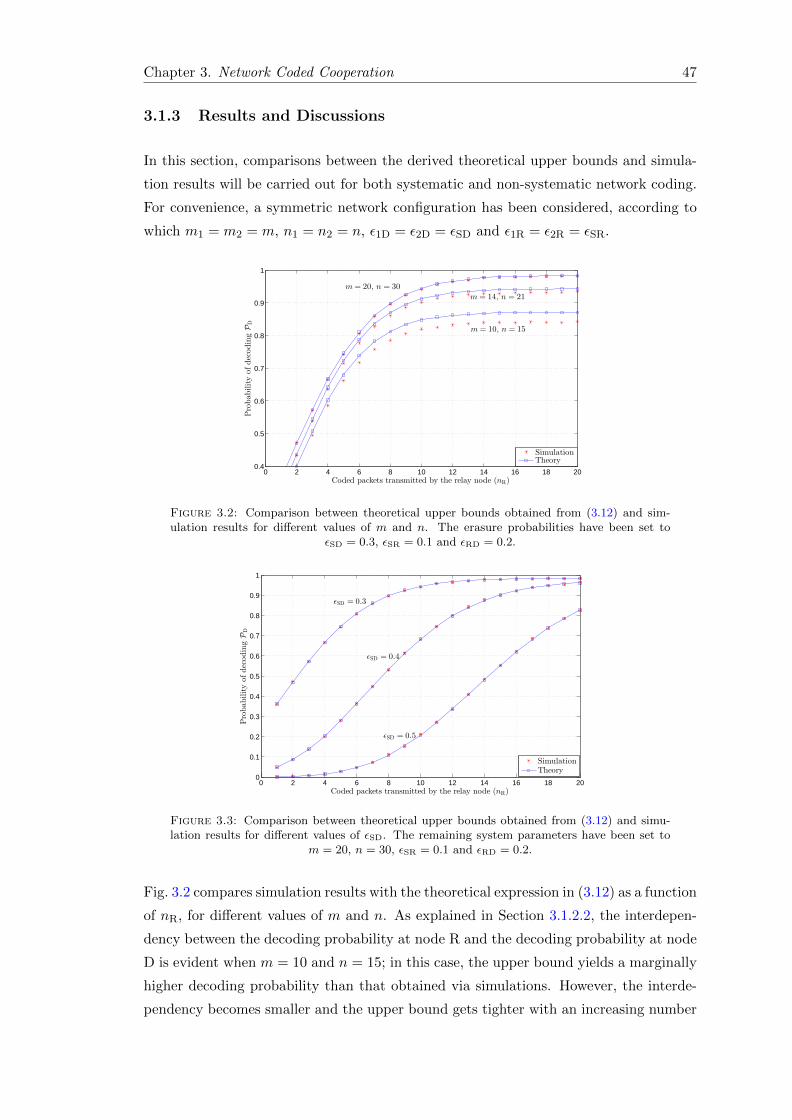
Chapter 3. Network Coded Cooperation 47
3.1.3 Results and Discussions
In this section, comparisons between the derived theoretical upper bounds and simula-
tion results will be carried out for both systematic and non-systematic network coding.
For convenience, a symmetric network configuration has been considered, according to
which m1 = m2 = m, n1 = n2 = n, ε1D = ε2D = εSD and ε1R = ε2R = εSR.
0 2 4 6 8 10 12 14 16 18 200.4
0.5
0.6
0.7
0.8
0.9
1
Coded packets transmitted by the relay node (nR)
ProbabilityofdecodingP
D
SimulationTheory
m = 14, n = 21
m = 10, n = 15
m = 20, n = 30
Figure 3.2: Comparison between theoretical upper bounds obtained from (3.12) and sim-ulation results for different values of m and n. The erasure probabilities have been set to
εSD = 0.3, εSR = 0.1 and εRD = 0.2.
0 2 4 6 8 10 12 14 16 18 200
0.1
0.2
0.3
0.4
0.5
0.6
0.7
0.8
0.9
1
Coded packets transmitted by the relay node (nR)
ProbabilityofdecodingP
D
SimulationTheory
ǫSD = 0.3
ǫSD = 0.5
ǫSD = 0.4
Figure 3.3: Comparison between theoretical upper bounds obtained from (3.12) and simu-lation results for different values of εSD. The remaining system parameters have been set to
m = 20, n = 30, εSR = 0.1 and εRD = 0.2.
Fig. 3.2 compares simulation results with the theoretical expression in (3.12) as a function
of nR, for different values of m and n. As explained in Section 3.1.2.2, the interdepen-
dency between the decoding probability at node R and the decoding probability at node
D is evident when m = 10 and n = 15; in this case, the upper bound yields a marginally
higher decoding probability than that obtained via simulations. However, the interde-
pendency becomes smaller and the upper bound gets tighter with an increasing number
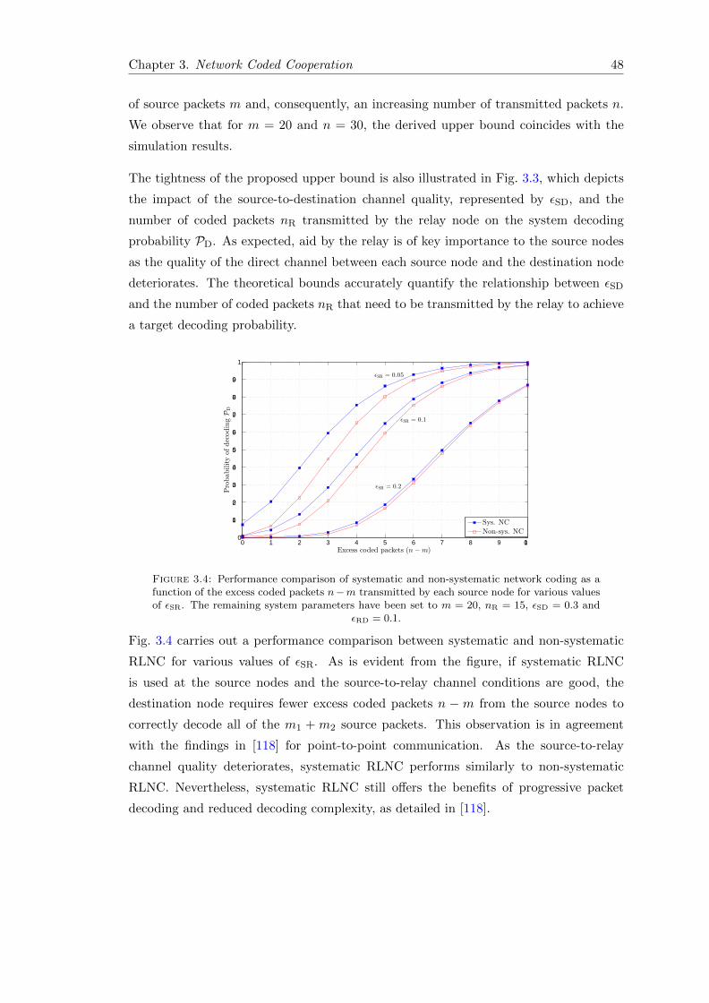
Chapter 3. Network Coded Cooperation 48
of source packets m and, consequently, an increasing number of transmitted packets n.
We observe that for m = 20 and n = 30, the derived upper bound coincides with the
simulation results.
The tightness of the proposed upper bound is also illustrated in Fig. 3.3, which depicts
the impact of the source-to-destination channel quality, represented by εSD, and the
number of coded packets nR transmitted by the relay node on the system decoding
probability PD. As expected, aid by the relay is of key importance to the source nodes
as the quality of the direct channel between each source node and the destination node
deteriorates. The theoretical bounds accurately quantify the relationship between εSD
and the number of coded packets nR that need to be transmitted by the relay to achieve
a target decoding probability.
0 1 2 3 4 5 6 7 8 9 100
0.1
0.2
0.3
0.4
0.5
0.6
0.7
0.8
0.9
1
Excess coded packets (n −m)
ProbabilityofdecodingP
D
Sys. NC
Non-sys. NC
ǫSR = 0.05
ǫSR = 0.2
ǫSR = 0.1
Figure 3.4: Performance comparison of systematic and non-systematic network coding as afunction of the excess coded packets n−m transmitted by each source node for various valuesof εSR. The remaining system parameters have been set to m = 20, nR = 15, εSD = 0.3 and
εRD = 0.1.
Fig. 3.4 carries out a performance comparison between systematic and non-systematic
RLNC for various values of εSR. As is evident from the figure, if systematic RLNC
is used at the source nodes and the source-to-relay channel conditions are good, the
destination node requires fewer excess coded packets n − m from the source nodes to
correctly decode all of the m1 + m2 source packets. This observation is in agreement
with the findings in [118] for point-to-point communication. As the source-to-relay
channel quality deteriorates, systematic RLNC performs similarly to non-systematic
RLNC. Nevertheless, systematic RLNC still offers the benefits of progressive packet
decoding and reduced decoding complexity, as detailed in [118].
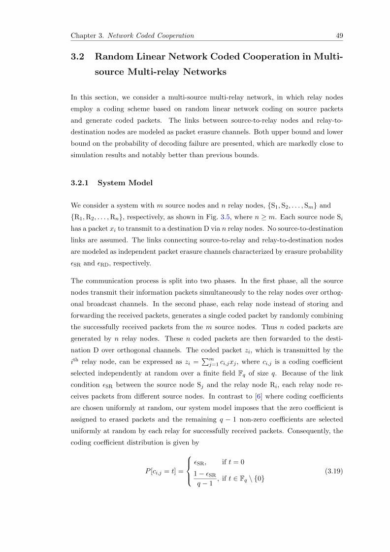
Chapter 3. Network Coded Cooperation 49
3.2 Random Linear Network Coded Cooperation in Multi-
source Multi-relay Networks
In this section, we consider a multi-source multi-relay network, in which relay nodes
employ a coding scheme based on random linear network coding on source packets
and generate coded packets. The links between source-to-relay nodes and relay-to-
destination nodes are modeled as packet erasure channels. Both upper bound and lower
bound on the probability of decoding failure are presented, which are markedly close to
simulation results and notably better than previous bounds.
3.2.1 System Model
We consider a system with m source nodes and n relay nodes, {S1,S2, . . . ,Sm} and
{R1,R2, . . . ,Rn}, respectively, as shown in Fig. 3.5, where n ≥ m. Each source node Si
has a packet xi to transmit to a destination D via n relay nodes. No source-to-destination
links are assumed. The links connecting source-to-relay and relay-to-destination nodes
are modeled as independent packet erasure channels characterized by erasure probability
εSR and εRD, respectively.
The communication process is split into two phases. In the first phase, all the source
nodes transmit their information packets simultaneously to the relay nodes over orthog-
onal broadcast channels. In the second phase, each relay node instead of storing and
forwarding the received packets, generates a single coded packet by randomly combining
the successfully received packets from the m source nodes. Thus n coded packets are
generated by n relay nodes. These n coded packets are then forwarded to the desti-
nation D over orthogonal channels. The coded packet zi, which is transmitted by the
ith relay node, can be expressed as zi =∑m
j=1 ci,jxj , where ci,j is a coding coefficient
selected independently at random over a finite field Fq of size q. Because of the link
condition εSR between the source node Sj and the relay node Ri, each relay node re-
ceives packets from different source nodes. In contrast to [6] where coding coefficients
are chosen uniformly at random, our system model imposes that the zero coefficient is
assigned to erased packets and the remaining q − 1 non-zero coefficients are selected
uniformly at random by each relay for successfully received packets. Consequently, the
coding coefficient distribution is given by
P [ci,j = t] =
εSR, if t = 0
1− εSR
q − 1, if t ∈ Fq \ {0}
(3.19)
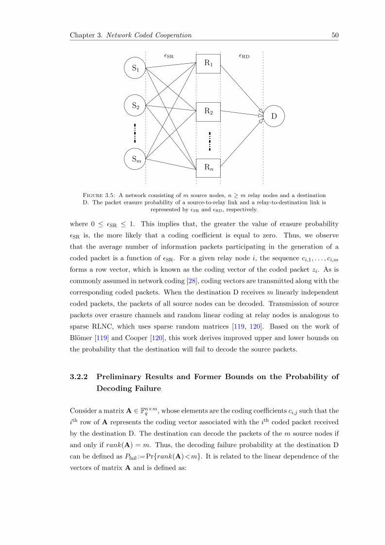
Chapter 3. Network Coded Cooperation 50
S1
S2
Sm
R1
R2
Rn
D
εSR εRD
Figure 3.5: A network consisting of m source nodes, n ≥ m relay nodes and a destinationD. The packet erasure probability of a source-to-relay link and a relay-to-destination link is
represented by εSR and εRD, respectively.
where 0 ≤ εSR ≤ 1. This implies that, the greater the value of erasure probability
εSR is, the more likely that a coding coefficient is equal to zero. Thus, we observe
that the average number of information packets participating in the generation of a
coded packet is a function of εSR. For a given relay node i, the sequence ci,1, . . . , ci,m
forms a row vector, which is known as the coding vector of the coded packet zi. As is
commonly assumed in network coding [28], coding vectors are transmitted along with the
corresponding coded packets. When the destination D receives m linearly independent
coded packets, the packets of all source nodes can be decoded. Transmission of source
packets over erasure channels and random linear coding at relay nodes is analogous to
sparse RLNC, which uses sparse random matrices [119, 120]. Based on the work of
Blomer [119] and Cooper [120], this work derives improved upper and lower bounds on
the probability that the destination will fail to decode the source packets.
3.2.2 Preliminary Results and Former Bounds on the Probability of
Decoding Failure
Consider a matrix A ∈ Fn×mq , whose elements are the coding coefficients ci,j such that the
ith row of A represents the coding vector associated with the ith coded packet received
by the destination D. The destination can decode the packets of the m source nodes if
and only if rank(A) = m. Thus, the decoding failure probability at the destination D
can be defined as Pfail :=Pr{rank(A)<m}. It is related to the linear dependence of the
vectors of matrix A and is defined as:
Chapter 3. Network Coded Cooperation 51
Definition 1. The vectors of matrix A ∈ Fn×mq are said to be linearly dependent if and
only if there exists a column vector x ∈ Fm×1q \{0} such that
Ax = 0. (3.20)
When there is no packet loss between the relay-to-destination channels, i.e., εRD = 0,
the probability that the elements of the ith row of matrix A add up to zero, i.e., ci,1 +
ci,2 + . . .+ ci,m = 0, is given by [119]
γm = q−1 + (1− q−1)(1− 1− εSR
1− q−1)m. (3.21)
Taking into account that matrix A consists of n rows, the probability Pr(Ax = 0) can
be obtained as
Pr(Ax = 0) = γnm =(q−1 + (1− q−1)(1− 1− εSR
1− q−1)m)n. (3.22)
The expected number of decoding failures at the destination D is given by the following
theorem, which is a straightforward adaptation of [119, Theorem 3.3], [120, Theorem 3]
to the system model under consideration.
Theorem 3.1. For a linear network coding scheme over m source nodes, n ≥ m relay
nodes and a single or multiple destinations, which are interconnected by links charac-
terized by packet erasure probabilities 0 ≤ εSR ≤ 1 and εRD = 0, the expectation of the
decoding failures can be obtained as
µ0(m,n)=E(Ax = 0)=1
q − 1
m∑w=1
(m
w
)(q − 1)wγnw (3.23)
where A ∈ Fn×mq is the coding matrix at a destination.
Following the same line of reasoning, a direct extension of (3.23) for εRD ≥ 0 has been
made in [59, Theorem 1] and was used to upper bound the probability of decoding
failure.
Corollary 3.2. The probability of decoding failure at a destination is bounded from
above as:
Pfail ≤1
q − 1
m∑w=1
(n
w
)(q − 1)w
[εRD + (1− εRD)γw
]n(3.24)
where m is the number of source nodes, n ≥ m is the number of relay nodes and εSR,
εRD represent the packet erasure probabilities between the network nodes.
Chapter 3. Network Coded Cooperation 52
However, (3.24) is only tight for limited values of erasures εSR and εRD, depending on
m, n and q. In particular, the upper bound takes values greater than 1 when either the
field size is big or the difference between the number of source and relay nodes is small.
This disparity between the probability of decoding failure and the upper bound will be
demonstrated in Section 3.2.4. In an effort to improve the tightness of (3.24), Seong et
al. proposed the selection of the minimum value between the upper bound in (3.24) and
1 [60]. A lower bound on the probability of decoding failure has also been obtained by
Seong in [59, Theorem 2]:
Theorem 3.3. Consider a network comprising m source nodes and n ≥ m relay nodes,
assume that links are modeled as packet erasure channels with erasure probabilities εSR
and εRD, and let A ∈ Fn×mq be the coding matrix at a destination node. The probability
of decoding failure Pfail is lower bounded by
Pfail ≥m∑k=1
(m
k
)((εSR + εRD − εSRεRD)n
)k(1− (εSR + εRD − εSRεRD)n)m−k. (3.25)
The bounds in (3.24) and (3.25) are used in [60] and [121]. For example, (3.24) is em-
ployed in [121] to evaluate the performance gains introduced by linear NC in a practical
network architecture for emergency communications. However, the following section will
derive new bounds, which are considerably tighter than the previous bounds and can
significantly improve the quality and accuracy of results presented in the literature.
3.2.3 Improved Bounds on the Probability of Decoding Failure
3.2.3.1 Upper bound
For εRD = 0, an upper bound on the decoding failure probability can be obtained by
extending and adapting [119, Theorem 6.3] as follows:
Lemma 3.4. Let A ∈ Fn×mq be the coding matrix at a destination node of a network
consisting of m source nodes and n relay nodes. If the internode erasure probabilities
are 0 ≤ εSR ≤ 1 and εRD = 0, the probability of decoding failure is upper bounded by
ηmax(m,n) = 1−m∏i=1
(1− βn−i+1max ) (3.26)
where βmax = max(εSR,1− εSR
q − 1) represents the maximum probability of obtaining an
element from Fq.
Chapter 3. Network Coded Cooperation 53
Proof. Let us assume that the first i−1 columns of A, denoted by A1,A2, . . . ,Ai−1, are
linearly independent. This implies that by using elementary column operations, matrix
A can be transformed into a matrix that contains an (i− 1)× (i− 1) identity matrix.
Without loss of generality, let us assume that the first i − 1 rows form the identity
matrix. The columns of this matrix represent the basis for the vector space spanned
by A1,A2, . . . ,Ai−1. Therefore, the probability that Ai is linearly independent from
A1,A2, . . . ,Ai−1 depends only on the last n−i+1 elements of Ai. This probability is
lower bounded by 1 − βn−i+1max , where βmax can be obtained by selecting the maximum
between the erasure probability and the probability of choosing a non-zero element
over the finite field Fq. Hence, matrix A contains an m × n non-singular matrix with
probability at least∏mi=1(1− βn−i+1
max ). As a result, the probability that matrix A does not
contain an invertible matrix and, consequently, a decoding failure will occur is upper
bounded by subtracting this product from one, which completes the proof.
Lemma 3.4 will be used to obtain a tighter upper bound on Pfail. Before we invoke it,
we shall first revisit (3.24) and rewrite it as:
Pfail ≤n∑n=0
(n
n
)εn−nRD (1− εRD)nµ0(m, n). (3.27)
This change is possible if [εRD + (1 − εRD)γw ]n is expanded into a sum, as per the
binomial theorem.
Theorem 3.5. For a network coding scheme over multi-source multi-relay networks,
composed of m source nodes and n relay nodes with packet erasures εSR and εRD, the
probability of decoding failure is upper bounded by
Pfail≤n∑n=0
(n
n
)εn−nRD (1− εRD)nmin{ηmax(m, n), µ0(m, n)}. (3.28)
Proof. As inferred from (3.27), the number of packet deliveries by the relays follows
the binomial distribution. If we employ Theorem 3.1 and Lemma 3.4 on the number of
received coded packets n, a tight upper bound can be obtained by taking the minimum
of outcomes and multiply with the probability distribution of n. Summing the resultant
quantity gives (3.28), which concludes the proof.
Remark 3.6. It is worth noting that the upper bound is not simply the minimum between
two cumulative probability distributions (CDFs), that is, the right-hand of (3.24) and
the CDF of (3.26) for all possible numbers of relay nodes. Instead, the right hand
of (3.24) has been rewritten in the form of (3.27), which enabled us to identify the
minimum between µ0 and ηmax for each possible number of relay nodes, and use it in
the computation of the CDF shown in (3.27).
Chapter 3. Network Coded Cooperation 54
3.2.3.2 Lower bound
The bound that was derived in [119, Theorem 6.3] was extended to an upper bound on
the probability that an n×m matrix A does not contain an invertible m× n matrix in
Lemma 3.4. The same approach can be followed to obtain a lower bound as follows:
Lemma 3.7. Let A ∈ Fn×mq be the coding matrix at a destination of a network consisting
of m source nodes and n relay nodes. If the internode erasure probabilities are 0 ≤ εSR ≤1 and εRD = 0, the probability of decoding failure is lower bounded by
ηmin(m,n) = 1−m∏i=1
(1− βn−i+1min ) (3.29)
where βmin = min(εSR,1− εSR
q − 1).
Proof. The proof follows exactly the same line of reasoning as that of Lemma 3.4.
An improved lower bound on Pfail can be obtained if the right-hand side of (8) is denoted
by P0(m,n) for εRD = 0, that is
P0(m,n) =m∑k=1
(m
k
)(εnSR)k(1− εnSR)m−k (3.30)
and then combined with (3.29) in Lemma 3.7. In particular:
Theorem 3.8. For a linear network coding scheme over m source nodes and n ≥ m
relay nodes, let εSR and εRD be the packet erasure probabilities of the internode links.
The probability of decoding failure is lower bounded by
Pfail≥n∑n=0
(m
n
)εn−nRD (1− εRD)nmax{ηmin(m, n), P0(m, n)}. (3.31)
Proof. In contrast to Theorem 3.5, here we employ Lemma 3.7 and (3.30) on the number
of received coded packets n, and we select the maximum of outcomes. The rest of the
proof follows the same reasoning as that presented in the proof of Theorem 3.5.
3.2.4 Results and Discussions
This section compares the analytical expressions of the proposed bounds to simulation
results. In addition, the proposed upper bound and lower bound, which shall be referred
to as UB-new and LB-new, are contrasted with the old bounds represented by (3.24)
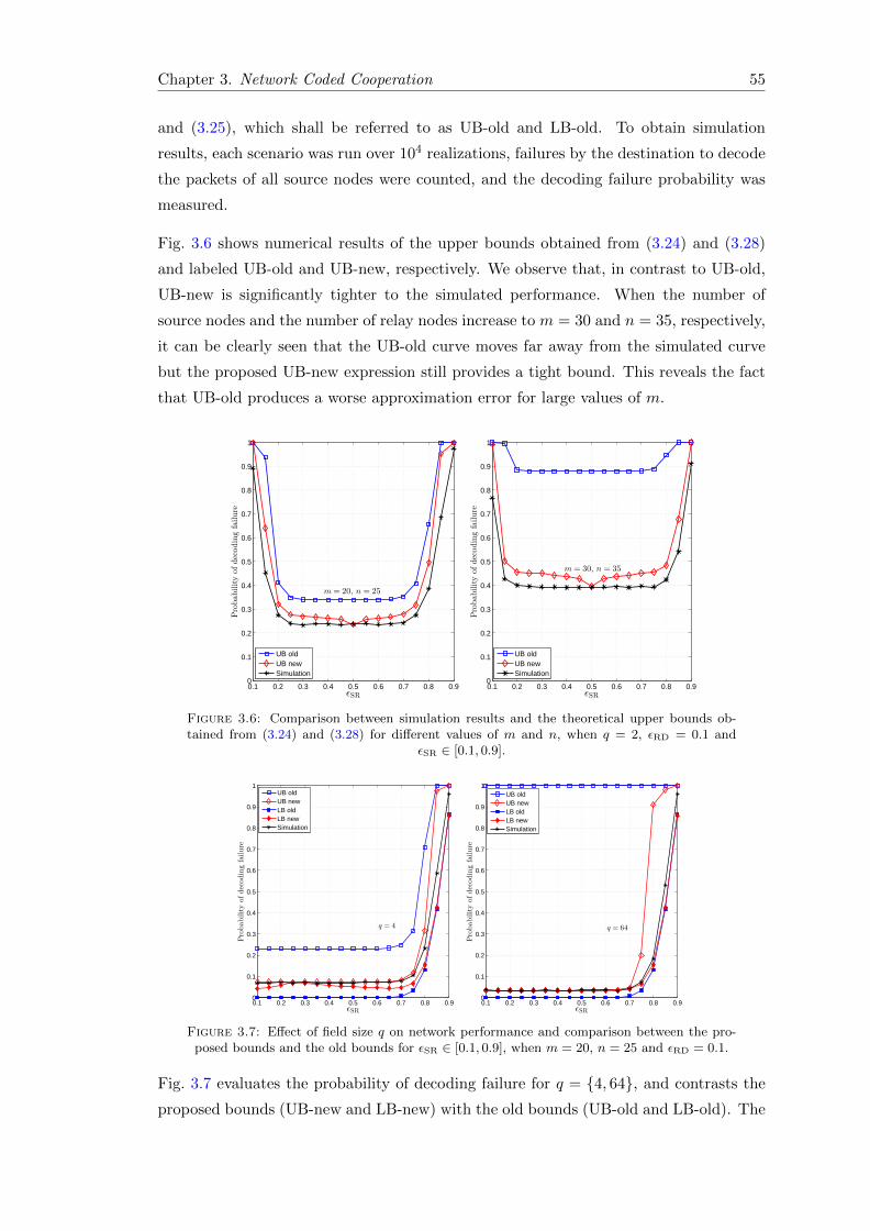
Chapter 3. Network Coded Cooperation 55
and (3.25), which shall be referred to as UB-old and LB-old. To obtain simulation
results, each scenario was run over 104 realizations, failures by the destination to decode
the packets of all source nodes were counted, and the decoding failure probability was
measured.
Fig. 3.6 shows numerical results of the upper bounds obtained from (3.24) and (3.28)
and labeled UB-old and UB-new, respectively. We observe that, in contrast to UB-old,
UB-new is significantly tighter to the simulated performance. When the number of
source nodes and the number of relay nodes increase to m = 30 and n = 35, respectively,
it can be clearly seen that the UB-old curve moves far away from the simulated curve
but the proposed UB-new expression still provides a tight bound. This reveals the fact
that UB-old produces a worse approximation error for large values of m.
0.1 0.2 0.3 0.4 0.5 0.6 0.7 0.8 0.90
0.1
0.2
0.3
0.4
0.5
0.6
0.7
0.8
0.9
1
ǫSR
Probabilityofdecodingfailure
UB oldUB newSimulation
0.1 0.2 0.3 0.4 0.5 0.6 0.7 0.8 0.90
0.1
0.2
0.3
0.4
0.5
0.6
0.7
0.8
0.9
1
ǫSR
Probabilityofdecodingfailure
UB oldUB newSimulation
m = 20, n = 25
m = 30, n = 35
Figure 3.6: Comparison between simulation results and the theoretical upper bounds ob-tained from (3.24) and (3.28) for different values of m and n, when q = 2, εRD = 0.1 and
εSR ∈ [0.1, 0.9].
0.1 0.2 0.3 0.4 0.5 0.6 0.7 0.8 0.90
0.1
0.2
0.3
0.4
0.5
0.6
0.7
0.8
0.9
1
ǫSR
Probabilityofdecodingfailure
UB oldUB newLB oldLB newSimulation
0.1 0.2 0.3 0.4 0.5 0.6 0.7 0.8 0.90
0.1
0.2
0.3
0.4
0.5
0.6
0.7
0.8
0.9
1
ǫSR
Probabilityofdecodingfailure
UB oldUB newLB oldLB newSimulation
q = 64q = 4
Figure 3.7: Effect of field size q on network performance and comparison between the pro-posed bounds and the old bounds for εSR ∈ [0.1, 0.9], when m = 20, n = 25 and εRD = 0.1.
Fig. 3.7 evaluates the probability of decoding failure for q = {4, 64}, and contrasts the
proposed bounds (UB-new and LB-new) with the old bounds (UB-old and LB-old). The
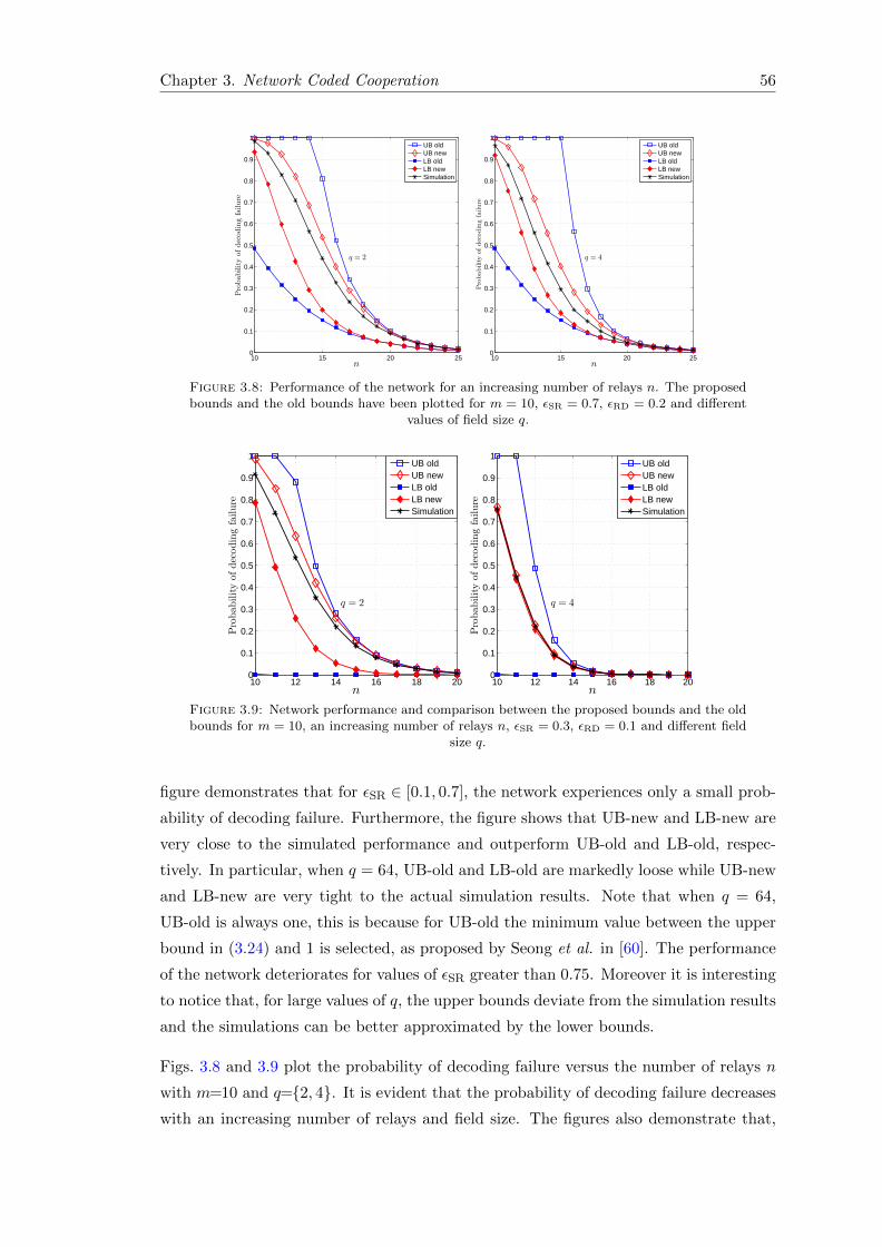
Chapter 3. Network Coded Cooperation 56
10 15 20 250
0.1
0.2
0.3
0.4
0.5
0.6
0.7
0.8
0.9
1
n
Probabilityofdecodingfailure
UB oldUB newLB oldLB newSimulation
10 15 20 250
0.1
0.2
0.3
0.4
0.5
0.6
0.7
0.8
0.9
1
n
Probabilityofdecodingfailure
UB oldUB newLB oldLB newSimulation
q = 4q = 2
Figure 3.8: Performance of the network for an increasing number of relays n. The proposedbounds and the old bounds have been plotted for m = 10, εSR = 0.7, εRD = 0.2 and different
values of field size q.
10 12 14 16 18 200
0.1
0.2
0.3
0.4
0.5
0.6
0.7
0.8
0.9
1
n
Probabilityofdecodingfailure
UB oldUB newLB oldLB newSimulation
10 12 14 16 18 200
0.1
0.2
0.3
0.4
0.5
0.6
0.7
0.8
0.9
1
n
Probabilityofdecodingfailure
UB oldUB newLB oldLB newSimulation
q = 4q = 2
Figure 3.9: Network performance and comparison between the proposed bounds and the oldbounds for m = 10, an increasing number of relays n, εSR = 0.3, εRD = 0.1 and different field
size q.
figure demonstrates that for εSR ∈ [0.1, 0.7], the network experiences only a small prob-
ability of decoding failure. Furthermore, the figure shows that UB-new and LB-new are
very close to the simulated performance and outperform UB-old and LB-old, respec-
tively. In particular, when q = 64, UB-old and LB-old are markedly loose while UB-new
and LB-new are very tight to the actual simulation results. Note that when q = 64,
UB-old is always one, this is because for UB-old the minimum value between the upper
bound in (3.24) and 1 is selected, as proposed by Seong et al. in [60]. The performance
of the network deteriorates for values of εSR greater than 0.75. Moreover it is interesting
to notice that, for large values of q, the upper bounds deviate from the simulation results
and the simulations can be better approximated by the lower bounds.
Figs. 3.8 and 3.9 plot the probability of decoding failure versus the number of relays n
with m=10 and q={2, 4}. It is evident that the probability of decoding failure decreases
with an increasing number of relays and field size. The figures also demonstrate that,
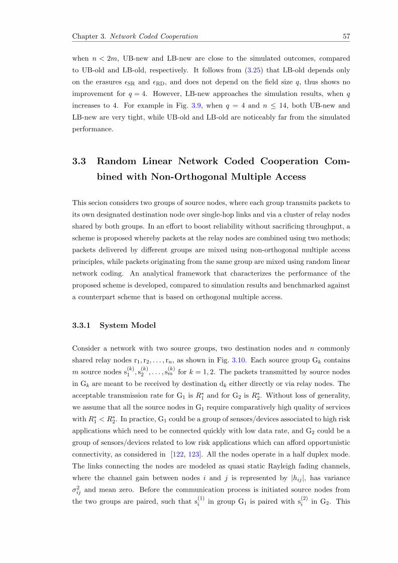
Chapter 3. Network Coded Cooperation 57
when n < 2m, UB-new and LB-new are close to the simulated outcomes, compared
to UB-old and LB-old, respectively. It follows from (3.25) that LB-old depends only
on the erasures εSR and εRD, and does not depend on the field size q, thus shows no
improvement for q = 4. However, LB-new approaches the simulation results, when q
increases to 4. For example in Fig. 3.9, when q = 4 and n ≤ 14, both UB-new and
LB-new are very tight, while UB-old and LB-old are noticeably far from the simulated
performance.
3.3 Random Linear Network Coded Cooperation Com-
bined with Non-Orthogonal Multiple Access
This secion considers two groups of source nodes, where each group transmits packets to
its own designated destination node over single-hop links and via a cluster of relay nodes
shared by both groups. In an effort to boost reliability without sacrificing throughput, a
scheme is proposed whereby packets at the relay nodes are combined using two methods;
packets delivered by different groups are mixed using non-orthogonal multiple access
principles, while packets originating from the same group are mixed using random linear
network coding. An analytical framework that characterizes the performance of the
proposed scheme is developed, compared to simulation results and benchmarked against
a counterpart scheme that is based on orthogonal multiple access.
3.3.1 System Model
Consider a network with two source groups, two destination nodes and n commonly
shared relay nodes r1, r2, . . . , rn, as shown in Fig. 3.10. Each source group Gk contains
m source nodes s(k)1 , s
(k)2 , . . . , s
(k)m for k = 1, 2. The packets transmitted by source nodes
in Gk are meant to be received by destination dk either directly or via relay nodes. The
acceptable transmission rate for G1 is R∗1 and for G2 is R∗2. Without loss of generality,
we assume that all the source nodes in G1 require comparatively high quality of services
with R∗1 < R∗2. In practice, G1 could be a group of sensors/devices associated to high risk
applications which need to be connected quickly with low data rate, and G2 could be a
group of sensors/devices related to low risk applications which can afford opportunistic
connectivity, as considered in [122, 123]. All the nodes operate in a half duplex mode.
The links connecting the nodes are modeled as quasi static Rayleigh fading channels,
where the channel gain between nodes i and j is represented by |hij |, has variance
σ2ij and mean zero. Before the communication process is initiated source nodes from
the two groups are paired, such that s(1)i in group G1 is paired with s
(2)i in G2. This
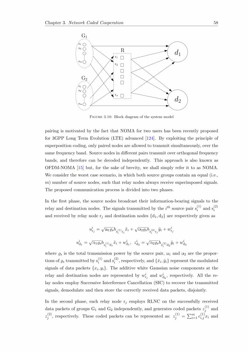
Chapter 3. Network Coded Cooperation 58
d1
d2
G1
G2
R
s1s2
sm
s1s2
sm
r1
r2
rn
Figure 3.10: Block diagram of the system model
pairing is motivated by the fact that NOMA for two users has been recently proposed
for 3GPP Long Term Evolution (LTE) advanced [124]. By exploiting the principle of
superposition coding, only paired nodes are allowed to transmit simultaneously, over the
same frequency band. Source nodes in different pairs transmit over orthogonal frequency
bands, and therefore can be decoded independently. This approach is also known as
OFDM-NOMA [15] but, for the sake of brevity, we shall simply refer it to as NOMA.
We consider the worst case scenario, in which both source groups contain an equal (i.e.,
m) number of source nodes, such that relay nodes always receive superimposed signals.
The proposed communication process is divided into two phases.
In the first phase, the source nodes broadcast their information-bearing signals to the
relay and destination nodes. The signals transmitted by the ith source pair s(1)i and s
(2)i
and received by relay node rj and destination nodes {d1,d2} are respectively given as
uirj =√a1%shs
(1)i rj
xi +√a2%shs
(2)i rj
yi + wirj
uid1=√a1%shs
(1)i d1
xi + wid1, zid2
=√a2%shs
(2)i d2
yi + wid2
where %s is the total transmission power by the source pair, a1 and a2 are the propor-
tions of %s transmitted by s(1)i and s
(2)i , respectively, and {xi, yi} represent the modulated
signals of data packets {xi, yi}. The additive white Gaussian noise components at the
relay and destination nodes are represented by wirj and widk , respectively. All the re-
lay nodes employ Successive Interference Cancellation (SIC) to recover the transmitted
signals, demodulate and then store the correctly received data packets, disjointly.
In the second phase, each relay node rj employs RLNC on the successfully received
data packets of groups G1 and G2 independently, and generates coded packets z(1)j and
z(2)j , respectively. These coded packets can be represented as: z
(1)j =
∑mi=1 c
(1)i,j xi and
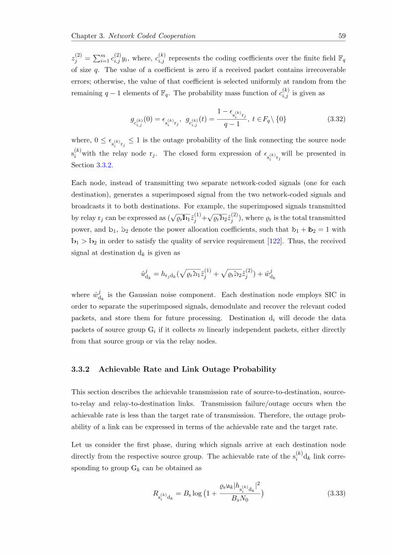
Chapter 3. Network Coded Cooperation 59
z(2)j =
∑mi=1 c
(2)i,j yi, where, c
(k)i,j represents the coding coefficients over the finite field Fq
of size q. The value of a coefficient is zero if a received packet contains irrecoverable
errors; otherwise, the value of that coefficient is selected uniformly at random from the
remaining q − 1 elements of Fq. The probability mass function of c(k)i,j is given as
gc(k)i,j
(0) = εs(k)i rj
, gc(k)i,j
(t) =1− ε
s(k)i rj
q − 1, t ∈Fq\ {0} (3.32)
where, 0 ≤ εs(k)i rj
≤ 1 is the outage probability of the link connecting the source node
s(k)i with the relay node rj . The closed form expression of ε
s(k)i rj
will be presented in
Section 3.3.2.
Each node, instead of transmitting two separate network-coded signals (one for each
destination), generates a superimposed signal from the two network-coded signals and
broadcasts it to both destinations. For example, the superimposed signals transmitted
by relay rj can be expressed as (√%rb1z
(1)j +√%rb2z
(2)j ), where %r is the total transmitted
power, and b1, b2 denote the power allocation coefficients, such that b1 + b2 = 1 with
b1 > b2 in order to satisfy the quality of service requirement [122]. Thus, the received
signal at destination dk is given as
ujdk = hrjdk(√%rb1z
(1)j +
√%rb2z
(2)j ) + wjdk
where wjdk is the Gaussian noise component. Each destination node employs SIC in
order to separate the superimposed signals, demodulate and recover the relevant coded
packets, and store them for future processing. Destination di will decode the data
packets of source group Gi if it collects m linearly independent packets, either directly
from that source group or via the relay nodes.
3.3.2 Achievable Rate and Link Outage Probability
This section describes the achievable transmission rate of source-to-destination, source-
to-relay and relay-to-destination links. Transmission failure/outage occurs when the
achievable rate is less than the target rate of transmission. Therefore, the outage prob-
ability of a link can be expressed in terms of the achievable rate and the target rate.
Let us consider the first phase, during which signals arrive at each destination node
directly from the respective source group. The achievable rate of the s(k)i dk link corre-
sponding to group Gk can be obtained as
Rs(k)i dk
= Bs log(1 +
%sak|hs(k)i dk|2
BsN0
)(3.33)
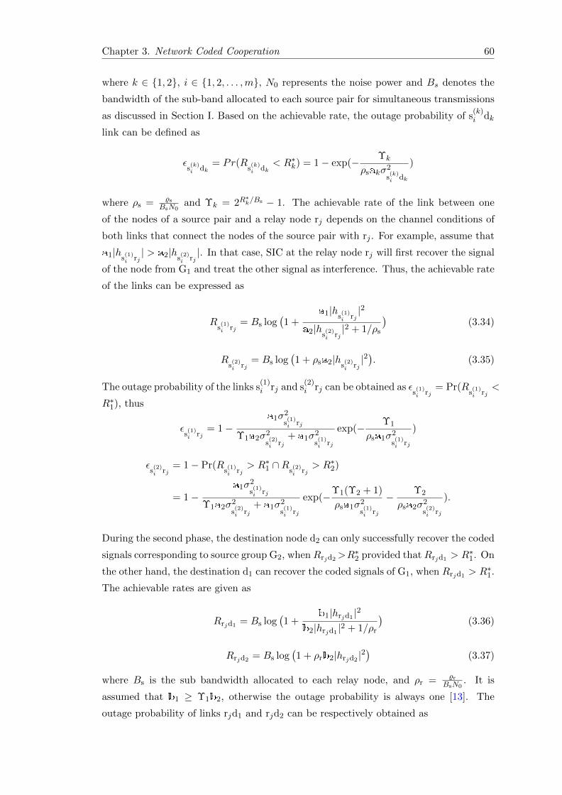
Chapter 3. Network Coded Cooperation 60
where k ∈ {1, 2}, i ∈ {1, 2, . . . ,m}, N0 represents the noise power and Bs denotes the
bandwidth of the sub-band allocated to each source pair for simultaneous transmissions
as discussed in Section I. Based on the achievable rate, the outage probability of s(k)i dk
link can be defined as
εs(k)i dk
= Pr(Rs(k)i dk
< R∗k) = 1− exp(− Υk
ρsakσ2
s(k)i dk
)
where ρs = %s
BsN0and Υk = 2R
∗k/Bs − 1. The achievable rate of the link between one
of the nodes of a source pair and a relay node rj depends on the channel conditions of
both links that connect the nodes of the source pair with rj . For example, assume that
a1|hs(1)i rj| > a2|hs
(2)i rj|. In that case, SIC at the relay node rj will first recover the signal
of the node from G1 and treat the other signal as interference. Thus, the achievable rate
of the links can be expressed as
Rs(1)i rj
= Bs log(1 +
a1|hs(1)i rj|2
a2|hs(2)i rj|2 + 1/ρs
)(3.34)
Rs(2)i rj
= Bs log(1 + ρsa2|hs
(2)i rj|2). (3.35)
The outage probability of the links s(1)i rj and s
(2)i rj can be obtained as ε
s(1)i rj
= Pr(Rs(1)i rj
<
R∗1), thus
εs(1)i rj
= 1−a1σ
2
s(1)i rj
Υ1a2σ2
s(2)i rj
+ a1σ2
s(1)i rj
exp(− Υ1
ρsa1σ2
s(1)i rj
)
εs(2)i rj
= 1− Pr(Rs(1)i rj
> R∗1 ∩Rs(2)i rj
> R∗2)
= 1−a1σ
2
s(1)i rj
Υ1a2σ2
s(2)i rj
+ a1σ2
s(1)i rj
exp(−Υ1(Υ2 + 1)
ρsa1σ2
s(1)i rj
− Υ2
ρsa2σ2
s(2)i rj
).
During the second phase, the destination node d2 can only successfully recover the coded
signals corresponding to source group G2, when Rrjd2>R∗2 provided that Rrjd1 > R∗1. On
the other hand, the destination d1 can recover the coded signals of G1, when Rrjd1 > R∗1.
The achievable rates are given as
Rrjd1 = Bs log(1 +
b1|hrjd1 |2
b2|hrjd1 |2 + 1/ρr
)(3.36)
Rrjd2 = Bs log(1 + ρrb2|hrjd2 |2
)(3.37)
where Bs is the sub bandwidth allocated to each relay node, and ρr = %r
BsN0. It is
assumed that b1 ≥ Υ1b2, otherwise the outage probability is always one [13]. The
outage probability of links rjd1 and rjd2 can be respectively obtained as
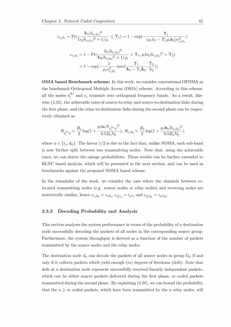
Chapter 3. Network Coded Cooperation 61
εrjd1 = Pr(b1|hrjd1 |2
b2|hrjd1 |2 + 1/ρr≤ Υ1) = 1− exp(− Υ1
(ρrb1 −Υ1ρrb2)σ2rjd1
)
εrjd2 = 1− Pr(b1|hrjd2 |2
b2|hrjd2 |2 + 1/ρr> Υ1, ρrb2|hrjd2 |2 > Υ2)
= 1− exp(− 1
ρrσ2rjd2
max(Υ1
b1 −Υ1b2,Υ2
b2)).
OMA based Benchmark scheme: In this work, we consider conventional OFDMA as
the benchmark Orthogonal Multiple Access (OMA) scheme. According to this scheme,
all the nodes s(k)i and rj transmit over orthogonal frequency bands. As a result, like-
wise (3.33), the achievable rates of source-to-relay and source-to-destination links during
the first phase, and the relay-to-destination links during the second phase can be respec-
tively obtained as
Rs(k)i u
=Bs
2log(1 +
%sak|hs(k)i u|2
0.5BsN0), Rrjdk =
Bs
2log(1 +
%rbk|hrjdk |2
0.5BsN0)
where u ∈ {rj , dk}. The factor 1/2 is due to the fact that, unlike NOMA, each sub-band
is now further split between two transmitting nodes. Note that, using the achievable
rates, we can derive the outage probabilities. These results can be further extended to
RLNC based analysis, which will be presented in the next section, and can be used as
benchmarks against the proposed NOMA based scheme.
In the remainder of the work, we consider the case where the channels between co-
located transmitting nodes (e.g. source nodes or relay nodes) and receiving nodes are
statistically similar, hence εrjdk = εrdk , εski rj= εskr and εski dk
= εskdk.
3.3.3 Decoding Probability and Analysis
This section analyses the system performance in terms of the probability of a destination
node successfully decoding the packets of all nodes in the corresponding source group.
Furthermore, the system throughput is derived as a function of the number of packets
transmitted by the source nodes and the relay nodes.
The destination node dk can decode the packets of all source nodes in group Gk if and
only if it collects packets which yield enough (m) degrees of freedoms (dofs). Note that
dofs at a destination node represent successfully received linearly independent packets,
which can be either source packets delivered during the first phase, or coded packets
transmitted during the second phase. By exploiting (3.28), we can bound the probability
that the n ≥ m coded packets, which have been transmitted by the n relay nodes, will
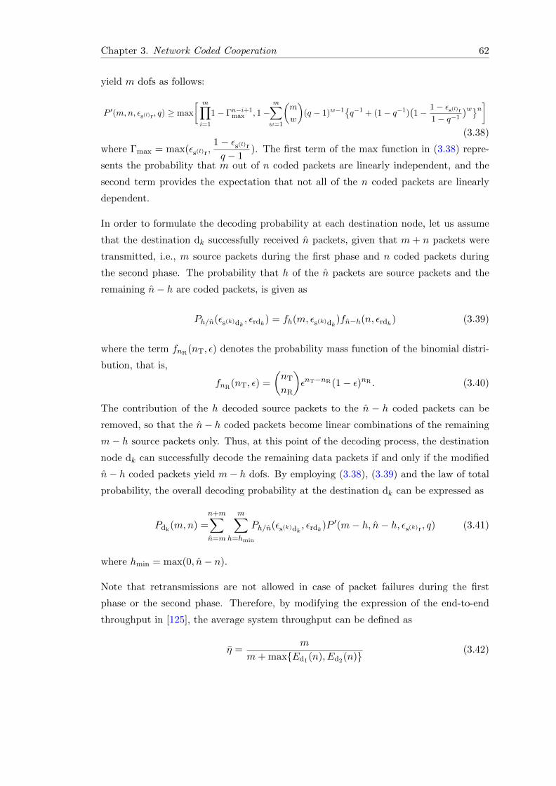
Chapter 3. Network Coded Cooperation 62
yield m dofs as follows:
P ′(m,n, εs(l)r, q) ≥ max
[ m∏i=1
1− Γn−i+1max , 1−
m∑w=1
(m
w
)(q − 1)w−1
{q−1 + (1− q−1)
(1− 1− εs(l)r
1− q−1
)w}n](3.38)
where Γmax = max(εs(l)r,1− εs(l)r
q − 1). The first term of the max function in (3.38) repre-
sents the probability that m out of n coded packets are linearly independent, and the
second term provides the expectation that not all of the n coded packets are linearly
dependent.
In order to formulate the decoding probability at each destination node, let us assume
that the destination dk successfully received n packets, given that m + n packets were
transmitted, i.e., m source packets during the first phase and n coded packets during
the second phase. The probability that h of the n packets are source packets and the
remaining n− h are coded packets, is given as
Ph/n(εs(k)dk, εrdk) = fh(m, εs(k)dk
)fn−h(n, εrdk) (3.39)
where the term fnR(nT, ε) denotes the probability mass function of the binomial distri-
bution, that is,
fnR(nT, ε) =
(nT
nR
)εnT−nR(1− ε)nR . (3.40)
The contribution of the h decoded source packets to the n − h coded packets can be
removed, so that the n− h coded packets become linear combinations of the remaining
m− h source packets only. Thus, at this point of the decoding process, the destination
node dk can successfully decode the remaining data packets if and only if the modified
n− h coded packets yield m− h dofs. By employing (3.38), (3.39) and the law of total
probability, the overall decoding probability at the destination dk can be expressed as
Pdk(m,n) =
n+m∑n=m
m∑h=hmin
Ph/n(εs(k)dk, εrdk)P ′(m− h, n− h, εs(k)r, q) (3.41)
where hmin = max(0, n− n).
Note that retransmissions are not allowed in case of packet failures during the first
phase or the second phase. Therefore, by modifying the expression of the end-to-end
throughput in [125], the average system throughput can be defined as
η =m
m+ max{Ed1(n), Ed2(n)}(3.42)
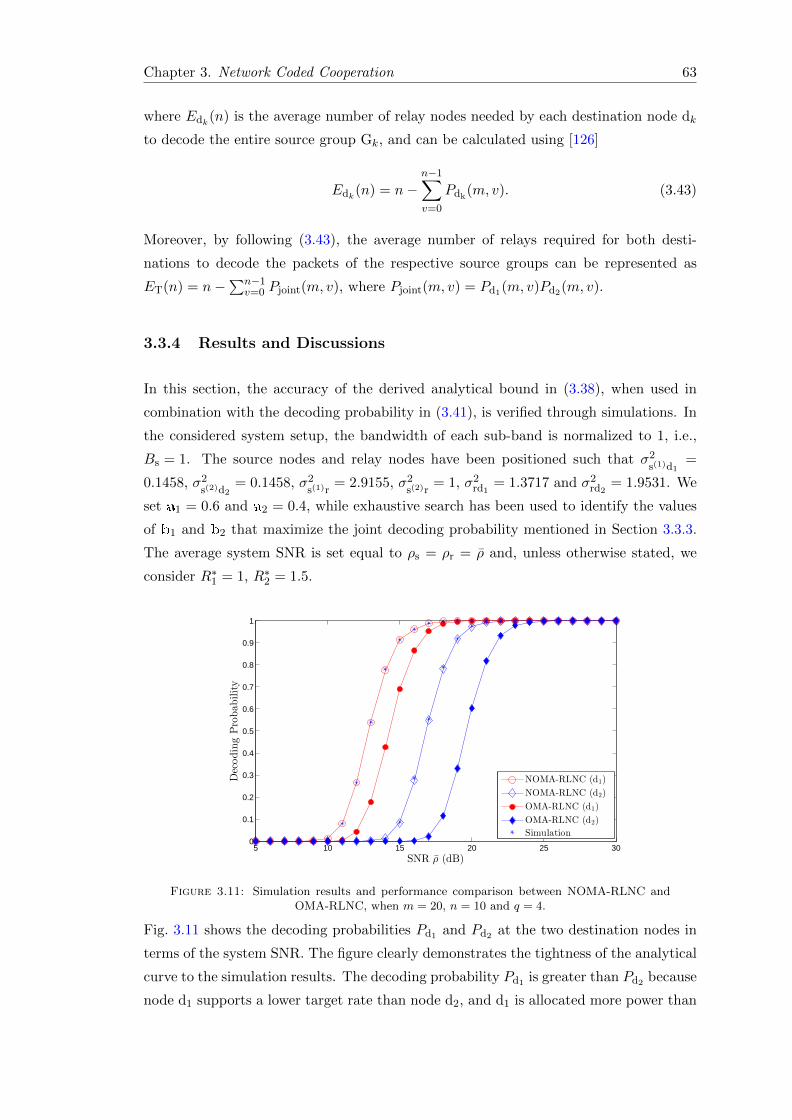
Chapter 3. Network Coded Cooperation 63
where Edk(n) is the average number of relay nodes needed by each destination node dk
to decode the entire source group Gk, and can be calculated using [126]
Edk(n) = n−n−1∑v=0
Pdk(m, v). (3.43)
Moreover, by following (3.43), the average number of relays required for both desti-
nations to decode the packets of the respective source groups can be represented as
ET(n) = n−∑n−1
v=0 Pjoint(m, v), where Pjoint(m, v) = Pd1(m, v)Pd2(m, v).
3.3.4 Results and Discussions
In this section, the accuracy of the derived analytical bound in (3.38), when used in
combination with the decoding probability in (3.41), is verified through simulations. In
the considered system setup, the bandwidth of each sub-band is normalized to 1, i.e.,
Bs = 1. The source nodes and relay nodes have been positioned such that σ2s(1)d1
=
0.1458, σ2s(2)d2
= 0.1458, σ2s(1)r
= 2.9155, σ2s(2)r
= 1, σ2rd1
= 1.3717 and σ2rd2
= 1.9531. We
set a1 = 0.6 and a2 = 0.4, while exhaustive search has been used to identify the values
of b1 and b2 that maximize the joint decoding probability mentioned in Section 3.3.3.
The average system SNR is set equal to ρs = ρr = ρ and, unless otherwise stated, we
consider R∗1 = 1, R∗2 = 1.5.
5 10 15 20 25 300
0.1
0.2
0.3
0.4
0.5
0.6
0.7
0.8
0.9
1
SNR ρ (dB)
DecodingProbability
NOMA-RLNC (d1)
NOMA-RLNC (d2)
OMA-RLNC (d1)
OMA-RLNC (d2)
Simulation
Figure 3.11: Simulation results and performance comparison between NOMA-RLNC andOMA-RLNC, when m = 20, n = 10 and q = 4.
Fig. 3.11 shows the decoding probabilities Pd1 and Pd2 at the two destination nodes in
terms of the system SNR. The figure clearly demonstrates the tightness of the analytical
curve to the simulation results. The decoding probability Pd1 is greater than Pd2 because
node d1 supports a lower target rate than node d2, and d1 is allocated more power than
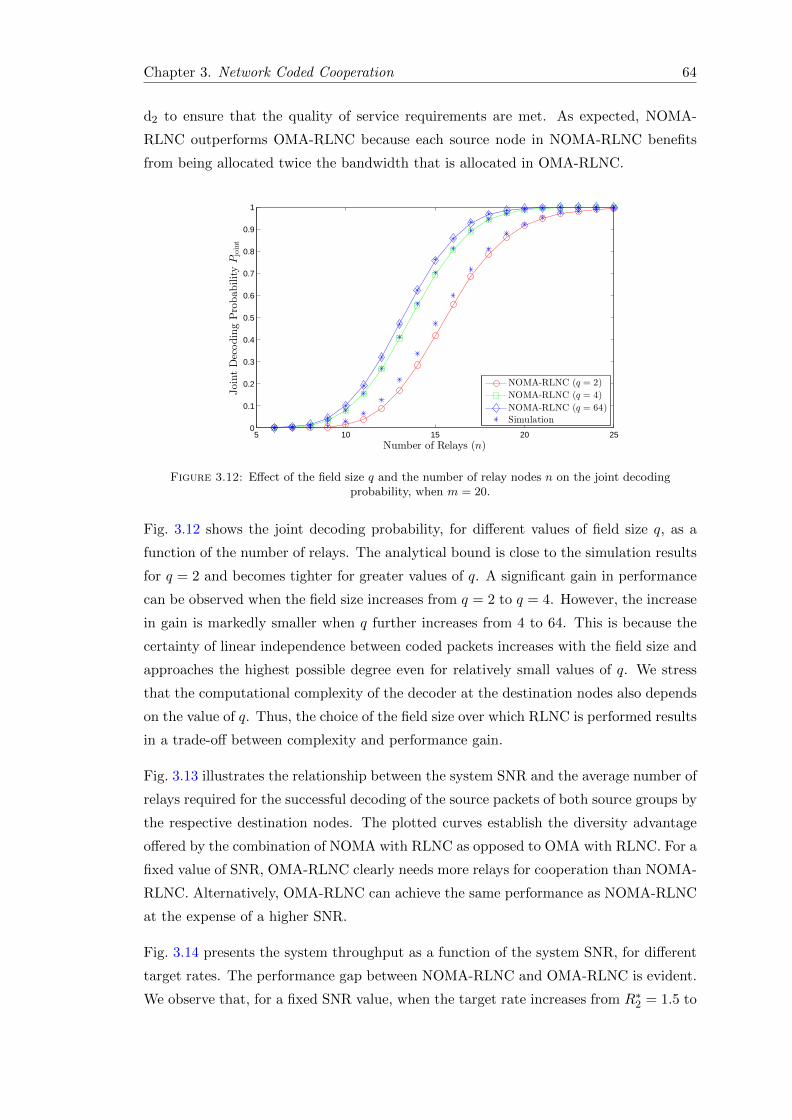
Chapter 3. Network Coded Cooperation 64
d2 to ensure that the quality of service requirements are met. As expected, NOMA-
RLNC outperforms OMA-RLNC because each source node in NOMA-RLNC benefits
from being allocated twice the bandwidth that is allocated in OMA-RLNC.
5 10 15 20 250
0.1
0.2
0.3
0.4
0.5
0.6
0.7
0.8
0.9
1
Number of Relays (n)
JointDecodingProbabilityPjoint
NOMA-RLNC (q = 2)
NOMA-RLNC (q = 4)
NOMA-RLNC (q = 64)
Simulation
Figure 3.12: Effect of the field size q and the number of relay nodes n on the joint decodingprobability, when m = 20.
Fig. 3.12 shows the joint decoding probability, for different values of field size q, as a
function of the number of relays. The analytical bound is close to the simulation results
for q = 2 and becomes tighter for greater values of q. A significant gain in performance
can be observed when the field size increases from q = 2 to q = 4. However, the increase
in gain is markedly smaller when q further increases from 4 to 64. This is because the
certainty of linear independence between coded packets increases with the field size and
approaches the highest possible degree even for relatively small values of q. We stress
that the computational complexity of the decoder at the destination nodes also depends
on the value of q. Thus, the choice of the field size over which RLNC is performed results
in a trade-off between complexity and performance gain.
Fig. 3.13 illustrates the relationship between the system SNR and the average number of
relays required for the successful decoding of the source packets of both source groups by
the respective destination nodes. The plotted curves establish the diversity advantage
offered by the combination of NOMA with RLNC as opposed to OMA with RLNC. For a
fixed value of SNR, OMA-RLNC clearly needs more relays for cooperation than NOMA-
RLNC. Alternatively, OMA-RLNC can achieve the same performance as NOMA-RLNC
at the expense of a higher SNR.
Fig. 3.14 presents the system throughput as a function of the system SNR, for different
target rates. The performance gap between NOMA-RLNC and OMA-RLNC is evident.
We observe that, for a fixed SNR value, when the target rate increases from R∗2 = 1.5 to
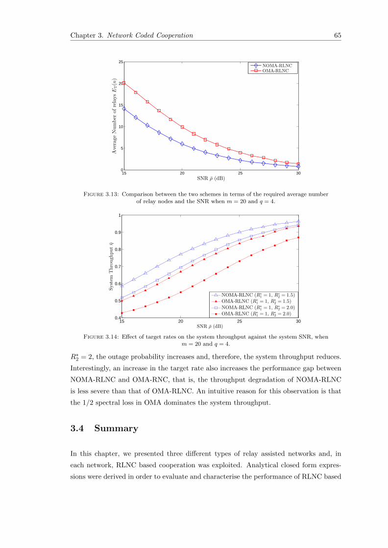
Chapter 3. Network Coded Cooperation 65
15 20 25 300
5
10
15
20
25
AverageNumber
ofrelaysE
T(n)
SNR ρ (dB)
NOMA-RLNCOMA-RLNC
Figure 3.13: Comparison between the two schemes in terms of the required average numberof relay nodes and the SNR when m = 20 and q = 4.
15 20 25 300.4
0.5
0.6
0.7
0.8
0.9
1
SNR ρ (dB)
System
Throughputη
NOMA-RLNC (R∗
1 = 1, R∗
2 = 1.5)OMA-RLNC (R∗
1 = 1, R∗
2 = 1.5)
NOMA-RLNC (R∗
1 = 1, R∗
2 = 2.0)OMA-RLNC (R∗
1 = 1, R∗
2 = 2.0)
Figure 3.14: Effect of target rates on the system throughput against the system SNR, whenm = 20 and q = 4.
R∗2 = 2, the outage probability increases and, therefore, the system throughput reduces.
Interestingly, an increase in the target rate also increases the performance gap between
NOMA-RLNC and OMA-RNC, that is, the throughput degradation of NOMA-RLNC
is less severe than that of OMA-RLNC. An intuitive reason for this observation is that
the 1/2 spectral loss in OMA dominates the system throughput.
3.4 Summary
In this chapter, we presented three different types of relay assisted networks and, in
each network, RLNC based cooperation was exploited. Analytical closed form expres-
sions were derived in order to evaluate and characterise the performance of RLNC based
Chapter 3. Network Coded Cooperation 66
cooperation, for each network. Simulation results confirmed the accuracy of the expres-
sions. The contributions made in this chapter can be summarised as follows:
• In Section 3.1, we studied the performance of a network comprising two source
nodes transmitting to a destination node via a relay node, where random linear
network coding is used both at the source nodes and the relay node. Upper bounds
on the probability of the destination node successfully decoding the packets of
both source nodes were derived for both systematic and non-systematic network
coding. Simulation results confirmed the validity of our theoretical analysis and
established that the upper bounds get tighter and accurately predict the system
decoding probability for an increasing number of transmitted coded packets by
the source nodes. Furthermore, we demonstrated that systematic network coding
can yield a similar or better performance than non-systematic network coding
depending on the quality of the uplink channels.
• In Section 3.2, we presented improved upper and lower bounds on the probability of
decoding failure in a multi-source multi-relay network, which employs RLNC. The
proposed analysis for counting failures provided significantly tighter bounds, which
outperform existing bounds, derived in [59]. Several examples, which considered
various numbers of source nodes and relay nodes, different field sizes and a range
of erasure probabilities, established the shortcomings of the existing bounds and
demonstrated the tightness of the proposed improved bounds. Finally, we asserted
that the proposed bounds can also be used to better estimate the performance of
systems employing sparse random linear network coding schemes, presented in the
literature.
• In Section 3.3, we investigated the benefits of NOMA-based multiplexing and
RLNC-based cooperative relaying in terms of decoding probability and system
throughput. Simulation results established the tightness of the derived expres-
sions. Comparisons emphasized the importance of network-coded cooperation and
demonstrated the impact of the field size on network performance. This work
showed that the combination of NOMA with RLNC can clearly provide a superior
performance, in terms of diversity gain and system throughput, than the combi-
nation of conventional OMA with RLNC.
Chapter 4
Random Linear Network Coding
for Secure Communication
Chapter 2 and Chapter 3 were focused on the development of mathematical frameworks
for the evaluation and characterisation of RLNC performance in multicast communica-
tion as well as cooperative communication. We have studied the robustness and useful-
ness of RLNC against erasure channels, and exhibited the effect of the finite field and the
number of cooperative relays on the overall decoding performance of networks. Finally,
we have also demonstrated the effect of multiple access schemes on the performance of
network coded cooperation.
In this chapter, we divert our attention from the reliability benefits of RLNC and in-
stead focus on the study and application of the inherent feature of RLNC for secure
communication. The chapter is mainly divided into two sections. Section 4.1 considers
a basic secrecy problem with conventional characters: Alice (legitimate transmitter),
Bob (legitimate receiver) and Eavesdropper (undesired receiver), where Alice employs
RLNC for the delivery of confidential message to Bob. In this section, we assess and for-
mulate the level of intrinsic secrecy provided by RLNC, in terms of intercept probability.
This work has been inspired by the methodology in [64] but differs in two major points.
Firstly, we have revisited the derivation of the intercept probability. More specifically,
the decoding probability of a receiver has been taken into account in our calculations.
Furthermore, key probability expressions have been revised to accurately reflect (i) the
effect of the size of the finite field over which network coding is performed, (ii) the im-
pact of a feedback link between the legitimate receiver and the transmitter, and (iii)
the fact that the number of transmitted coded packets cannot be infinite in practice.
The second difference is that [64] proposed an optimization model with respect to the
number of source packets composing a message. However, the number of source packets
67
Chapter 4. RLNC for Secure communication 68
and, by extension, their length are often dictated by the provided service. Our objec-
tive is to minimize the intercept probability by optimizing the number of transmitted
coded packets, under delay and reliability constraints. As part of the optimization pro-
cess, we prove that awareness of the existence of an eavesdropper is not required by the
transmitter and the legitimate receiver.
Section 4.2 focuses to investigate the potential of relay-aided networks that combine
RLNC with opportunistic relaying, with or without cooperative jamming, in securely
and reliably delivering confidential messages. To this end, we consider four different relay
selection protocols, we analyze their outage behaviour and we quantify the proportion of
the message that could leak to the eavesdropper with a certain probability by the time the
legitimate destination has decoded the entire message with a target probability. To the
best of our knowledge, only few studies that exploit the properties of RLNC in PLS are
available. For example, in order to enhance the secrecy of cooperative transmissions in
sensor networks, fountain-coding aided cooperative relaying with jamming was proposed
in [52]. Similarly to this work, we employ RLNC on the application layer. In contrast
to [52], where only one relay has been considered for aiding the source in its transmission
to the destination, we consider the complete problem of selecting a relay or a relay-
jammer pair from the set of available nodes. Furthermore, relays do not only perform
decode-and-forward, as in [52], but also linearly combine successfully received data
packets. Other notable differences from [52] include the derivation of the probability
that a fraction of data will leak to the eavesdropper, as opposed to the total amount of
transmitted data, and the investigation of the impact of both the finite field size used by
RLNC and the adopted forward error correction and modulation scheme on the security
and reliability of the network.
4.1 The Intercept Probability of RLNC
This section considers a network comprising a transmitter, which employs random lin-
ear network coding to encode a message, a legitimate receiver, which can decode the
message if it gathers a sufficient number of linearly independent coded packets, and an
eavesdropper. Closed-form expressions for the probability of the eavesdropper intercept-
ing enough coded packets to decode the message are derived. Transmission with and
without feedback is studied. Furthermore, an optimization model that minimizes the
intercept probability under delay and reliability constraints is presented.
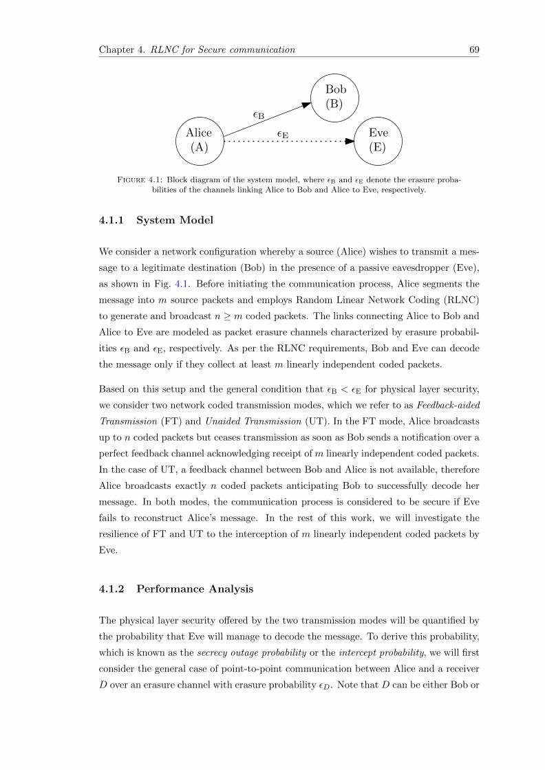
Chapter 4. RLNC for Secure communication 69
Alice(A)
Bob(B)
Eve(E)
εB
εE
Figure 4.1: Block diagram of the system model, where εB and εE denote the erasure proba-bilities of the channels linking Alice to Bob and Alice to Eve, respectively.
4.1.1 System Model
We consider a network configuration whereby a source (Alice) wishes to transmit a mes-
sage to a legitimate destination (Bob) in the presence of a passive eavesdropper (Eve),
as shown in Fig. 4.1. Before initiating the communication process, Alice segments the
message into m source packets and employs Random Linear Network Coding (RLNC)
to generate and broadcast n ≥ m coded packets. The links connecting Alice to Bob and
Alice to Eve are modeled as packet erasure channels characterized by erasure probabil-
ities εB and εE, respectively. As per the RLNC requirements, Bob and Eve can decode
the message only if they collect at least m linearly independent coded packets.
Based on this setup and the general condition that εB < εE for physical layer security,
we consider two network coded transmission modes, which we refer to as Feedback-aided
Transmission (FT) and Unaided Transmission (UT). In the FT mode, Alice broadcasts
up to n coded packets but ceases transmission as soon as Bob sends a notification over a
perfect feedback channel acknowledging receipt of m linearly independent coded packets.
In the case of UT, a feedback channel between Bob and Alice is not available, therefore
Alice broadcasts exactly n coded packets anticipating Bob to successfully decode her
message. In both modes, the communication process is considered to be secure if Eve
fails to reconstruct Alice’s message. In the rest of this work, we will investigate the
resilience of FT and UT to the interception of m linearly independent coded packets by
Eve.
4.1.2 Performance Analysis
The physical layer security offered by the two transmission modes will be quantified by
the probability that Eve will manage to decode the message. To derive this probability,
which is known as the secrecy outage probability or the intercept probability, we will first
consider the general case of point-to-point communication between Alice and a receiver
D over an erasure channel with erasure probability εD. Note that D can be either Bob or
Chapter 4. RLNC for Secure communication 70
Eve, i.e., D ∈ {B,E}. If Alice transmits n ≥ m coded packets and the receiver retrieves
n coded packets, where m ≤ n ≤ n, the probability that the receiver will successfully
decode the m source packets can be obtained using (2.2), given as
P (n,m) =m−1∏i=0
[1− q−(n−i)
],
where q is the size of the finite field over which network coding operations are performed.
Let X be a random variable that represents the number of transmitted coded packets
for which the receiver can decode the m source packets. The Cumulative Distribution
Function (CDF) of X describes the probability that the receiver will decode the m source
packets after nT coded packets have been transmitted, where m ≤ nT ≤n. This CDF
can be obtained by employing (2.20) that is averaging P (n,m) over all valid values of
n, represented as
FD(nT) = Pr {X ≤ nT} =
nT∑n=m
(nT
n
)(1− εD)nεnT−n
D P (n,m). (4.1)
The probability that the receiver will decode the m source packets when the nT-th coded
packet has been transmitted, but not earlier, is given by the Probability Mass Function
(PMF) of X, which can be derived as follows:
fD(nT) = Pr {X = nT} =
FD(nT)− FD(nT − 1), if m < nT ≤ n
FD(m), if nT = m.(4.2)
Let us now return our focus to the considered network configuration operating in the FT
mode. Recall that Bob sends an acknowledgment to Alice when he receives m linearly
independent coded packets and can thus decode the source message. The intercept
probability can be expressed as the sum of two constituent probabilities:
P FTint (n) = PBE(n) + PE(n). (4.3)
The first term of the sum in (4.3), PBE(n), denotes the probability that both Bob and
Eve will decode the message. This can happen if Bob decodes the message only after the
nT-th coded packet has been transmitted, while Eve has already decoded the message
or decodes it concurrently with Bob. Invoking the definitions in (4.1) and (4.2), and
considering all possible values of nT, we can express PBE(n) as
PBE(n) =
n∑nT=m
fB(nT)FE(nT). (4.4)
Chapter 4. RLNC for Secure communication 71
The second term of the sum in (4.3), PE(n), represents the probability that Eve will
be successful in decoding the message but Bob will fail to decode it after Alice has
transmitted the complete sequence of n coded packets. Using the CDF of the number
of coded packets delivered by Alice to Eve and Bob, respectively, we can write PE(n) as
follows:
PE(n) = FE(n) [ 1− FB(n) ] . (4.5)
We should stress that (4.4) and (4.5) are exact only if the sequence of coded packets
delivered over the Alice-to-Bob link is independent of the sequence delivered over the
Alice-to-Eve link. This is a common hypothesis in the literature of broadcast networks,
e.g., [64] and [113], and is valid for a non-vanishing product between the number of
coded packets transmitted over a channel and the erasure probability of that channel.
The accuracy of (4.3) will also be demonstrated in Section 4.1.4.
In the case of UT, a feedback channel is not available between Bob and Alice, therefore
Alice transmits the complete sequence of n coded packets uninterruptedly. Therefore,
the intercept probability is simply equal to the probability that Eve will decode the
message after Alice has transmitted n coded packets. Using the definition of the CDF
in (4.1), we obtain
P UTint (n) = FE(n). (4.6)
Manipulation of the expression for P FTint (n), as shown in Appendix B, and subtraction
of P UTint (n) from it, yields
P FTint (n)− P UT
int (n) = −n∑
nT=m+1
fE(nT)FB(nT − 1). (4.7)
Expression (4.7) measures the loss in the intercept capability of Eve or, equivalently, the
gain in secrecy by Bob, if Bob can acknowledge the decoding of the source message to
Alice using a feedback channel.
Remark 4.1. In this work, we assume that Alice has knowledge of the average channel
conditions, characterized by the erasure probability, between her and Bob. If Alice could
sense the instantaneous channel quality and transmitted coded packets only when the
channel quality warranted their error-free delivery to Bob, as in [64], [127], the equivalent
erasure probability of the link between Alice and Bob would be εB = 0. In that case,
Alice could generate exactly m linearly independent coded packets in a deterministic
manner, as opposed to random, and forward them to Bob. As a result, the intercept
probability would reduce to (1 − εE)m regardless the transmission mode. This remark
concurs with the conclusion of [64] that an arbitrarily small intercept probability can be
achieved by increasing the value of m, but at the cost of increased delay.
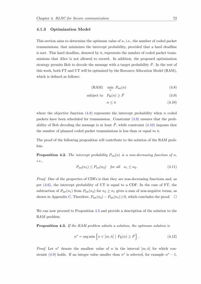
Chapter 4. RLNC for Secure communication 72
4.1.3 Optimization Model
This section aims to determine the optimum value of n, i.e., the number of coded packet
transmissions, that minimizes the intercept probability, provided that a hard deadline
is met. This hard deadline, denoted by n, represents the number of coded packet trans-
missions that Alice is not allowed to exceed. In addition, the proposed optimization
strategy permits Bob to decode the message with a target probability P . In the rest of
this work, both FT and UT will be optimized by the Resource Allocation Model (RAM),
which is defined as follows:
(RAM) minn
Pint(n) (4.8)
subject to FB(n) ≥ P (4.9)
n ≤ n (4.10)
where the objective function (4.8) represents the intercept probability when n coded
packets have been scheduled for transmission. Constraint (4.9) ensures that the prob-
ability of Bob decoding the message is at least P , while constraint (4.10) imposes that
the number of planned coded packet transmissions is less than or equal to n.
The proof of the following proposition will contribute to the solution of the RAM prob-
lem.
Proposition 4.2. The intercept probability Pint(n) is a non-decreasing function of n,
i.e.,
Pint(n1) ≤ Pint(n2) for all n1 ≤ n2. (4.11)
Proof. One of the properties of CDFs is that they are non-decreasing functions and, as
per (4.6), the intercept probability of UT is equal to a CDF. In the case of FT, the
subtraction of Pint(n1) from Pint(n2) for n2 ≥ n1 gives a sum of non-negative terms, as
shown in Appendix C. Therefore, Pint(n2)− Pint(n1)≥0, which concludes the proof.
We can now proceed to Proposition 4.3 and provide a description of the solution to the
RAM problem.
Proposition 4.3. If the RAM problem admits a solution, the optimum solution is
n∗ = arg min{n ∈ [m, n]
∣∣ FB(n) ≥ P}. (4.12)
Proof. Let n∗ denote the smallest value of n in the interval [m, n] for which con-
straint (4.9) holds. If an integer value smaller than n∗ is selected, for example n∗ − 1,
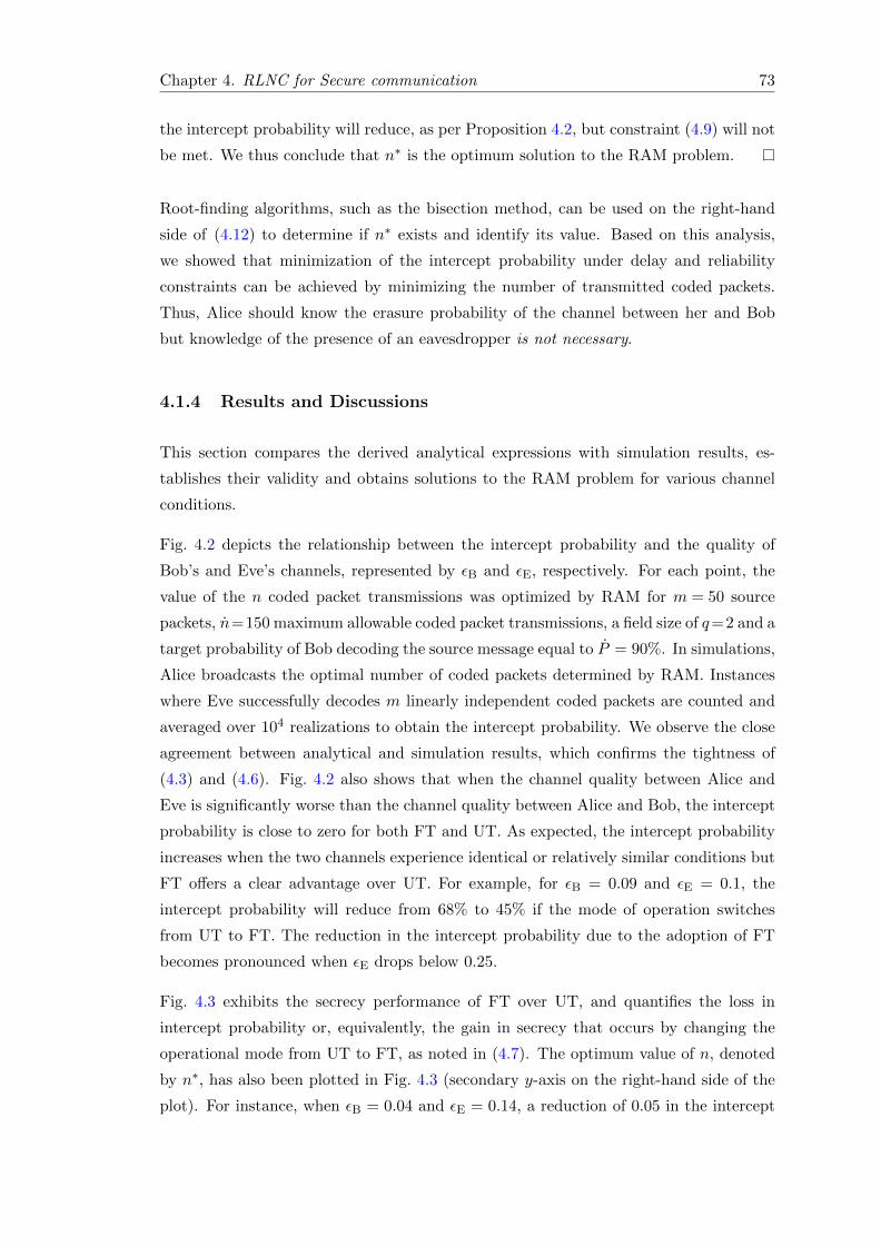
Chapter 4. RLNC for Secure communication 73
the intercept probability will reduce, as per Proposition 4.2, but constraint (4.9) will not
be met. We thus conclude that n∗ is the optimum solution to the RAM problem.
Root-finding algorithms, such as the bisection method, can be used on the right-hand
side of (4.12) to determine if n∗ exists and identify its value. Based on this analysis,
we showed that minimization of the intercept probability under delay and reliability
constraints can be achieved by minimizing the number of transmitted coded packets.
Thus, Alice should know the erasure probability of the channel between her and Bob
but knowledge of the presence of an eavesdropper is not necessary.
4.1.4 Results and Discussions
This section compares the derived analytical expressions with simulation results, es-
tablishes their validity and obtains solutions to the RAM problem for various channel
conditions.
Fig. 4.2 depicts the relationship between the intercept probability and the quality of
Bob’s and Eve’s channels, represented by εB and εE, respectively. For each point, the
value of the n coded packet transmissions was optimized by RAM for m = 50 source
packets, n=150 maximum allowable coded packet transmissions, a field size of q=2 and a
target probability of Bob decoding the source message equal to P = 90%. In simulations,
Alice broadcasts the optimal number of coded packets determined by RAM. Instances
where Eve successfully decodes m linearly independent coded packets are counted and
averaged over 104 realizations to obtain the intercept probability. We observe the close
agreement between analytical and simulation results, which confirms the tightness of
(4.3) and (4.6). Fig. 4.2 also shows that when the channel quality between Alice and
Eve is significantly worse than the channel quality between Alice and Bob, the intercept
probability is close to zero for both FT and UT. As expected, the intercept probability
increases when the two channels experience identical or relatively similar conditions but
FT offers a clear advantage over UT. For example, for εB = 0.09 and εE = 0.1, the
intercept probability will reduce from 68% to 45% if the mode of operation switches
from UT to FT. The reduction in the intercept probability due to the adoption of FT
becomes pronounced when εE drops below 0.25.
Fig. 4.3 exhibits the secrecy performance of FT over UT, and quantifies the loss in
intercept probability or, equivalently, the gain in secrecy that occurs by changing the
operational mode from UT to FT, as noted in (4.7). The optimum value of n, denoted
by n∗, has also been plotted in Fig. 4.3 (secondary y-axis on the right-hand side of the
plot). For instance, when εB = 0.04 and εE = 0.14, a reduction of 0.05 in the intercept
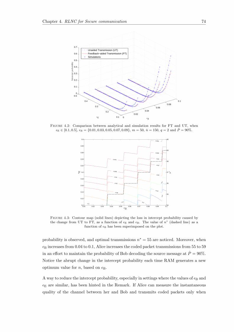
Chapter 4. RLNC for Secure communication 74
0
0.02
0.04
0.06
0.08
0.1
0.1
0.2
0.3
0.4
0.50
0.1
0.2
0.3
0.4
0.5
0.6
0.7
ǫBǫE
Intercep
tprobability
Unaided Transmission (UT)Feedback−aided Transmission (FT)Simulations
Figure 4.2: Comparison between analytical and simulation results for FT and UT, whenεE ∈ [0.1, 0.5], εB = {0.01, 0.03, 0.05, 0.07, 0.09}, m = 50, n = 150, q = 2 and P = 90%.
−0.2
−0.2
−0.15
−0.1−0.1
−0.1
−0.05
−0.05
−0.02
−0.02
−0.01
−0.01
−0.005
−0.005
−0.001
−0.001
0.01 0.02 0.03 0.04 0.05 0.06 0.07 0.08 0.09 0.10.1
0.12
0.14
0.16
0.18
0.2
0.22
0.24
0.26
0.28
0.3
ǫB
ǫE
54
55
56
57
58
59
60
n∗
Figure 4.3: Contour map (solid lines) depicting the loss in intercept probability caused bythe change from UT to FT, as a function of εE and εB. The value of n∗ (dashed line) as a
function of εB has been superimposed on the plot.
probability is observed, and optimal transmissions n∗ = 55 are noticed. Moreover, when
εB increases from 0.04 to 0.1, Alice increases the coded packet transmissions from 55 to 59
in an effort to maintain the probability of Bob decoding the source message at P = 90%.
Notice the abrupt change in the intercept probability each time RAM generates a new
optimum value for n, based on εB.
A way to reduce the intercept probability, especially in settings where the values of εB and
εE are similar, has been hinted in the Remark. If Alice can measure the instantaneous
quality of the channel between her and Bob and transmits coded packets only when
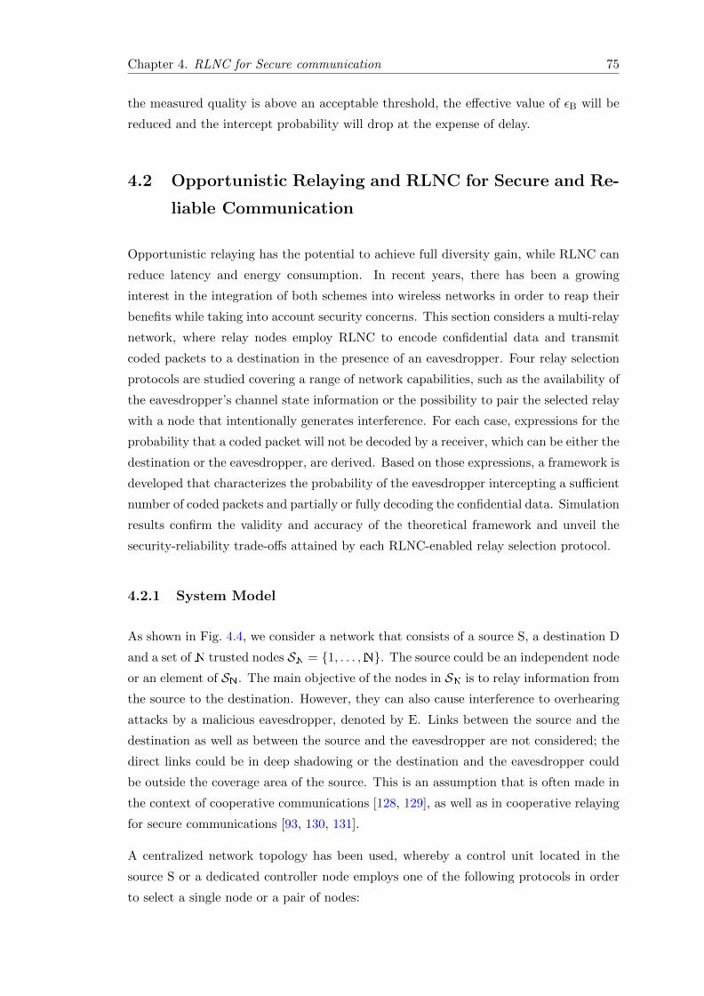
Chapter 4. RLNC for Secure communication 75
the measured quality is above an acceptable threshold, the effective value of εB will be
reduced and the intercept probability will drop at the expense of delay.
4.2 Opportunistic Relaying and RLNC for Secure and Re-
liable Communication
Opportunistic relaying has the potential to achieve full diversity gain, while RLNC can
reduce latency and energy consumption. In recent years, there has been a growing
interest in the integration of both schemes into wireless networks in order to reap their
benefits while taking into account security concerns. This section considers a multi-relay
network, where relay nodes employ RLNC to encode confidential data and transmit
coded packets to a destination in the presence of an eavesdropper. Four relay selection
protocols are studied covering a range of network capabilities, such as the availability of
the eavesdropper’s channel state information or the possibility to pair the selected relay
with a node that intentionally generates interference. For each case, expressions for the
probability that a coded packet will not be decoded by a receiver, which can be either the
destination or the eavesdropper, are derived. Based on those expressions, a framework is
developed that characterizes the probability of the eavesdropper intercepting a sufficient
number of coded packets and partially or fully decoding the confidential data. Simulation
results confirm the validity and accuracy of the theoretical framework and unveil the
security-reliability trade-offs attained by each RLNC-enabled relay selection protocol.
4.2.1 System Model
As shown in Fig. 4.4, we consider a network that consists of a source S, a destination D
and a set of N trusted nodes SN = {1, . . . ,N}. The source could be an independent node
or an element of SN. The main objective of the nodes in SN is to relay information from
the source to the destination. However, they can also cause interference to overhearing
attacks by a malicious eavesdropper, denoted by E. Links between the source and the
destination as well as between the source and the eavesdropper are not considered; the
direct links could be in deep shadowing or the destination and the eavesdropper could
be outside the coverage area of the source. This is an assumption that is often made in
the context of cooperative communications [128, 129], as well as in cooperative relaying
for secure communications [93, 130, 131].
A centralized network topology has been used, whereby a control unit located in the
source S or a dedicated controller node employs one of the following protocols in order
to select a single node or a pair of nodes:
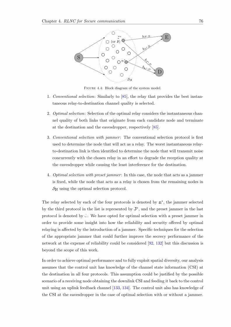
Chapter 4. RLNC for Secure communication 76
E
D
S
hJ∗ ,E
hn∗ ,E
hJ ∗,D
hn∗,D
J∗
(or J)
n∗
SN
Figure 4.4: Block diagram of the system model.
1. Conventional selection: Similarly to [85], the relay that provides the best instan-
taneous relay-to-destination channel quality is selected.
2. Optimal selection: Selection of the optimal relay considers the instantaneous chan-
nel quality of both links that originate from each candidate node and terminate
at the destination and the eavesdropper, respectively [85].
3. Conventional selection with jammer : The conventional selection protocol is first
used to determine the node that will act as a relay. The worst instantaneous relay-
to-destination link is then identified to determine the node that will transmit noise
concurrently with the chosen relay in an effort to degrade the reception quality at
the eavesdropper while causing the least interference for the destination.
4. Optimal selection with preset jammer : In this case, the node that acts as a jammer
is fixed, while the node that acts as a relay is chosen from the remaining nodes in
SN using the optimal selection protocol.
The relay selected by each of the four protocols is denoted by n∗, the jammer selected
by the third protocol in the list is represented by J∗, and the preset jammer in the last
protocol is denoted by J. We have opted for optimal selection with a preset jammer in
order to provide some insight into how the reliability and security offered by optimal
relaying is affected by the introduction of a jammer. Specific techniques for the selection
of the appropriate jammer that could further improve the secrecy performance of the
network at the expense of reliability could be considered [92, 132] but this discussion is
beyond the scope of this work.
In order to achieve optimal performance and to fully exploit spatial diversity, our analysis
assumes that the control unit has knowledge of the channel state information (CSI) at
the destination in all four protocols. This assumption could be justified by the possible
scenario of a receiving node obtaining the downlink CSI and feeding it back to the control
unit using an uplink feedback channel [133, 134]. The control unit also has knowledge of
the CSI at the eavesdropper in the case of optimal selection with or without a jammer.
Chapter 4. RLNC for Secure communication 77
Note that this is a common assumption in the physical-layer security literature [86, 135].
For example, the eavesdropper’s CSI can be known if the eavesdropper is part of the
network of legitimate receivers when unclassified data are broadcast, but is treated as an
unauthorized receiver when confidential data are transmitted. Even if an eavesdropper is
never destined to receive any type of transmitted data, its presence can still be detected
from power leaked via its antenna port while in receiving mode [136].
The delivery of a confidential message by the source to the destination using oppor-
tunistic relaying is divided into two phases. In the first phase, the source broadcasts the
message and the candidate relay nodes operate in receiving mode. In this work, we study
the impact that the RLNC-enabled relay selection schemes have on the leakage and re-
liability of information broadcast by the relay nodes. For this reason, we assume that
at the end of the first phase all of the relays have successfully received the message. For
example, the source could employ RLNC to segment the message into multiple packets
and encode them. The source would then broadcast randomly generated coded packets
until all receiving nodes in SN have reconstructed the message. Alternatively, the source
could transmit coded packets until one of the nodes in SN has received the message; the
nodes in SN could then use short-range communication to exchange packets until all
nodes have knowledge of the message. Given that, all the nodes in SN are trusted nodes
and there are no direct links available between the source and the eavesdropper node,
delivery of the broadcast message is considered to be secure during the first phase of
communication. In the second phase, each node in SN divides the message into m data
packets. Based on the adopted relay selection protocol, the control unit instructs the
chosen relay n∗ to employ RLNC on the data packets and generate a coded packet. The
coded packet is further processed by the transmission scheme at the physical layer of the
relay. The transmission scheme, which involves forward error correction and modulation
techniques, can be accurately characterized by a signal-to-noise ratio (SNR) threshold,
denoted by ρth, as described in [137–139]. This process is repeated up to n times and,
thus, up to n coded packets are transmitted; each time, the appropriate relay is selected
from SN, depending on the instantaneous channel conditions. Both the destination D
and the eavesdropper E collect coded packets and use them to construct local decoding
matrices. If m linearly independent coded packets are received, the rank of the decoding
matrix will be m. This implies that the m data packets can be decoded and the entire
message can be reconstructed. If the destination decodes the message before the set
deadline of n transmissions, it sends a notification to the control unit to terminate the
relay selection and packet transmission process.
The relay-to-destination links and the relay-to-eavesdropper links have been modeled as
independent but not identically distributed (i.n.i.d) quasi-static Rayleigh fading chan-
nels. The channel gain between nodes i and j, denoted by |hi,j |, remains constant
Chapter 4. RLNC for Secure communication 78
for the duration of a coded packet but changes independently from packet to packet.
The variance of the fading distribution is given by σ2i,j = E
{|hi,j |2
}= d
−αi,ji,j , where
E{|hi,j |2
}represents the expected value of |hi,j |2, and di,j and αi,j are the Euclidean
distance and the path loss exponent between the two nodes, respectively. Furthermore,
links are impaired by additive white Gaussian noise with zero mean and variance N0.
The instantaneous SNR of the link between i and j is represented as ρi,j = %i|hi,j |2/N0,
where %i is the transmitted power of node i. The probability density function of ρi,j is
equal to [140]
fρi,j (ρ) = Pr(ρi,j = ρ) = λi,je−ρλi,j (4.13)
where λi,j = 1/E {ρi,j}. The cumulative density function of ρi,j can be obtained as
follows
Fρi,j (ρth) = Pr(ρi,j ≤ ρth) = 1− e−ρthλi,j . (4.14)
Both the destination and the eavesdropper in the considered system model apply the
Gaussian elimination method on their respective decoding matrices to compute their
rank and decode the source message. The objective of the destination is to decodes
the entire message, i.e., all of the m data packets. Traditionally, the communication
process is deemed to be secure if the eavesdropper fails to decodes the message [64].
By contrast, this work assumes that the probability of the eavesdropper decoding the
received coded packets and recovering even a subset of the m data packets should be
very small. We shall refer to the probability of the eavesdropper retrieving at least τ of
the m data packets as τ -intercept probability and we will evaluate it in Section 4.2.3.
However, we will first investigate the impact of the considered relay selection protocols
on the capability of the system to reliably and securely relay confidential messages in
Section 4.2.2.
4.2.2 Relay Selection and Outage Analysis
This section describes the relay selection protocols in greater detail, and characterizes
their performance in terms of the outage probability at the destination D and the outage
probability at the eavesdropper E. The outage probability is the probability that the
instantaneous signal-to-interference-plus-noise ratio (SINR) at a receiving node, either
D or E, will drop below a predefined threshold ρth due to an event, e.g., deep fading
or interference. The outage probability at the destination D and the eavesdropper E,
denoted by εD and εE, respectively, can be expressed as
εD = Pr(SINRn∗,D ≤ ρth) (4.15)
Chapter 4. RLNC for Secure communication 79
εE = Pr(SINRn∗,E ≤ ρth) (4.16)
where n∗ represents the selected relay. As established in [137] for Rayleigh fading chan-
nels and extended in [138] and [139] for other channel models, the outage probability is
a very tight approximation of the packet error probability, if the value of ρth accurately
reflects the employed modulation and coding scheme. For example, ρth = 5.89 dB for
uncoded BPSK and ρth =−0.983 dB for BPSK combined with a typical convolutional
code [137] over Rayleigh fading channels. Analytical expressions of εD and εE are derived
in this section, which first considers the protocols that only use opportunistic relaying
and then focuses on the protocols that combine relaying with jamming.
4.2.2.1 Relay selection protocols without jammer
Conventional selection
This protocol only considers the channel quality of the relay-to-destination link. A relay
n∗ is selected from SN, such that
n∗ = arg maxn∈SN
ρn,D. (4.17)
Owing to the fact that no interference is introduced by a jammer, the SINR at the
destination D and the SINR at the eavesdropper E are SINRn∗,D =ρn∗,D and SINRn∗,E =
ρn∗,E, respectively. The outage probability εD can be obtained by considering the joint
probability of every node in SN being the selected relay and its link being in outage,
that is,
εD =
N∑n=1
Pr[(n∗ = n)∩ (ρn,D ≤ ρth)
]. (4.18)
If we take into account that the channels are statistically independent and that ρn,D
follows the distribution given in (4.13), we can use order statistics [141] and obtain
Pr(n∗ = n) =
∞∫0
N∏i=1,i 6=n
Pr(ρi,D ≤ x)fρn,D(x) dx
=
∞∫0
N∏i=1,i 6=n
(1− e−xλi,D
)fρn,D(x) dx.
(4.19)
Chapter 4. RLNC for Secure communication 80
The joint probability in (4.18) can be obtained from (4.19) by setting the upper limit of
the integral in (4.19) to ρth, resulting in
εD =
N∑n=1
ρth∫0
N∏i 6=n
(1− e−xλi,D
)fρn,D(x) dx. (4.20)
Using the multinomial identity [142], the product of terms in (4.20) can be expanded as
followsN∏i 6=n
(1− e−xλi,D) =
N−1∑m=0
∑Sm⊆SN\n|Sm|=m
(−1)me−x∑i∈Sm λi,D (4.21)
where the inner sum in (4.21) is over all possible sets Sm of size m that are subsets
of SN but exclude the node n. Substituting (4.21) into (4.20) and solving the integral
leads to
εD =
N∑n=1
N−1∑m=0
∑Sm⊆SN\n|Sm|=m
(−1)mλn,D∑
i∈Sm
λi,D + λn,D
[1− e−ρth(
∑i∈Sm λi,D+λn,D)
]. (4.22)
Following the same line of thought, the outage probability at the eavesdropper E can be
obtained as follows
εE =
N∑n=1
Pr(n∗ = n)Pr(ρn,E ≤ ρth) (4.23)
because ρn,D, which determines Pr(n∗ = n) is independent of ρn,E. Based on (4.14), we
have
Pr(ρn,E ≤ ρth) = 1− e−ρthλn,E (4.24)
therefore, expression (4.23) assumes the form
εE =N∑n=1
∞∫0
N∏i 6=n,
(1− e−xλi,D
)(1− e−ρthλn,E
)dx. (4.25)
Invoking (4.21) and solving the integral gives the following closed form expression
εE =N∑n=1
N−1∑m=0
∑Sm⊆SN\n|Sm|=m
(−1)mλn,D∑
i∈Sm
λi,D + λn,D
(1− e−ρthλn,E
). (4.26)
Optimal selection
This protocol is deemed ‘optimal’ because it exploits knowledge of the eavesdropper’s
CSI and achieves the maximum secrecy capacity [92]. Therefore, this work uses optimal
Chapter 4. RLNC for Secure communication 81
selection as a benchmark protocol and compares its performance to that of the other
three protocols. According to this protocol, the relay n∗ is selected such that
n∗ = arg maxn∈SN
(ρn,Dρn,E
). (4.27)
The outage probability at the destination can be obtained from the general expression
(4.18) if the probability of the selected relay being a particular node is expressed as
Pr(n∗ = n) =
∞∫0
∞∫0
I1(x, y)fρn,D(x)fρn,E(y) dx dy (4.28)
where
I1(x, y) =N∏i=1i 6=n
Pr
(ρi,Dρi,E≤ x
y
). (4.29)
If we set Λi =λi,Dλi,E
, expression (4.29) can be rewritten as [86]
I1(x, y) =
N∏i=1i 6=n
xΛixΛi + y
. (4.30)
Using partial fraction expansion and simplifying the resultant expression, (4.30) assumes
the form
I1(x, y) = 1−N∑i=1i 6=n
yΘi
xΛi + y(4.31)
where Θi is the partial fraction coefficient and is equal to
Θi =∏
k/∈{n,i}
−ΛkΛi − Λk
, for Λk 6= Λi. (4.32)
Substituting (4.28) into (4.18) and taking into account that ρn,D should not exceed ρth
gives
εD =N∑n=1
∞∫0
ρth∫0
I1(x, y)fρn,D(x)fρn,E(y) dx dy. (4.33)
Chapter 4. RLNC for Secure communication 82
Invoking [143, eq. (3.352.1)] and the relationships in [144, Section 4.2], we obtain
εD =N∑n=1
1− e−ρthλn,D +∑j 6=n
Θjλn,Ee−ρth(λn,D−Λjλn,E)
[E1
((α2 + 1)λn,Dρth
){Λjρth
α2−
Λjλn,Dα2
2
}+ e−ρthα2λn,DE1(ρthλn,D)
Λjλn,Dα2
2
− Λjλn,Dα2(α2 + 1)
e−ρth(α2+1)λn,D
]−
Θjλn,Dλn,EΛjα2
1
{ln
(1 +
α1
β1
)− α1
λn,E
}(4.34)
where α1 = λn,E −λn,DΛj
, α2 =Λjλn,Eλn,D
− 1, β1 =λn,DΛj
and E1 is the exponential integral,
as defined in [143].
The value of ρn,E in optimal relay selection affects the probability that a node will be
selected to act as a relay. As a result, and in contrast to (4.23), the outage probability at
the eavesdropper has to be expressed as the summation of joint probabilities, as follows
εE =
N∑n=1
Pr[(n∗ = n)∩ (ρn,E ≤ ρth)
]. (4.35)
Taking into account (4.28) and recalling that the value of ρn,E needs to be upper bounded
by ρth, we obtain
εE =
N∑n=1
ρth∫0
∞∫0
I1(x, y)fρn,D(x)fρn,E(y) dx dy. (4.36)
Derivation of an analytical expression for εE requires a similar approach to that in (4.34),
and leads to
εE =N∑n=1
1− e−ρthλn,E+∑j 6=n
Θjλn,Dλn,EΛjα2
1
[E1
(λn,Eρth
)−(1 + α1ρth)e−α1ρthE1(β1ρth)
− α1
λn,E
(1− e−ρthλn,E
)+ ln
(1 +
α1
β1
)].
(4.37)
4.2.2.2 Relay selection protocols with jammer
In an effort to increase the outage probability at the eavesdropper, a jammer can be
employed by the two aforementioned protocols. The selection mechanism of the jammer
and its impact on the outage probability at the destination and at the eavesdropper are
investigated in this subsection.
Chapter 4. RLNC for Secure communication 83
Conventional selection with jammer
This protocol is based on a joint relay-jammer pair selection scheme. Similarly to con-
ventional selection, this protocol first selects a relay n∗ from SN that provides the best
instantaneous SNR at the destination. Subsequently, one of the remaining nodes in SN is
selected to act as a jammer, such that it causes the least interference to the destination.
The pair selection scheme can be described by the following expressions
n∗ = arg maxn∈SN
ρn,D (4.38)
J∗ = arg minj∈SN\n∗
ρj,D. (4.39)
The SINR at the destination and the SINR at the eavesdropper are given by
SINRn∗,D =ρn∗,D
ρJ∗,D + 1(4.40)
SINRn∗,E =ρn∗,E
ρJ∗,E + 1. (4.41)
respectively. Clearly, both SINRn∗,D and SINRn∗,E depend on the selected nodes n∗ and
J∗.
The outage probability at the destination should consider the joint probability of a node
n being the relay, a different node m being the jammer, and the SINR at the destination
not exceeding the SNR threshold ρth, for all possible values of n and m. Therefore, εD
can be written as
εD =N∑n=1
N∑m6=n
Pr
[(n∗=n)
⋂(J∗=m)
⋂(ρn,D
ρm,D+1≤ ρth
)]. (4.42)
Taking into account that the instantaneous SNR of the jammer-to-destination channel
cannot be greater than the instantaneous SNR of the relay-to-destination channel, and
that the two channels are independent, we can express the joint probability of selecting
a relay-jammer pair as follows
Pr[(n∗=n)
⋂(J∗=m)
]=
∞∫0
ρn,D∫0
I2(x, y)fρm,D(y)fρn,D(x) dy dx (4.43)
where
I2(x, y) =N−2∏
i 6=n,i 6=mPr(y ≤ ρi,D ≤ x). (4.44)
Chapter 4. RLNC for Secure communication 84
Invoking (4.14), I2(x, y) assumes the form
I2(x, y) =N−2∏
i 6=n,i 6=m
(e−yλi,D − e−xλi,D
)(4.45)
which can be rewritten as
I2(x, y) =
N−2∑w=0
∑X=SN\{n,m}Sw⊆X ,Sw⊆X|Sw|=w
(−1)we−x∑i∈Swλi,D−y
∑j∈Swλj,D (4.46)
using the multinomial identity. Substituting (4.43) into (4.42) and properly setting the
limits of the two integrals gives
εD =N∑n=1
N∑m6=n
δ∫0
(y+1)ρth∫y
I2(x, y)fρn,D(x)fρm,D(y) dx dy (4.47)
where δ =∞ for ρth ≥ 1, and δ = ρth1−ρth
otherwise. Solving the integrals, we obtain
εD =N∑n=1
N∑m 6=n
N−2∑w=0
∑X=SN\{n,m}Sw⊆X ,Sw⊆X|Sw|=w
(−1)wλn,D λm,D δn,m (4.48)
where
δn,m =
1
cnλD− e−ρthcn
cncn,m, for ρth ≥ 1
1−e− ρthλD
1−ρthcnλD
− eρthcn
[1−e
−ρthcn,m1−ρth
cncn,m
], for ρth < 1
and cn =(∑
i∈Swλi,D + λn,D), cm =
(∑j∈Swλj,D + λm,D
), cn,m = (ρthcn + cm), λD =∑
N
k=1 λk,D.
Due to the fact that the process of selecting the relay and the jammer is independent of
the eavesdropper’s CSI, the outage probability at the eavesdropper can be obtained as
follows
εE =N∑n=1
N∑m 6=n
Pr[(n∗=n)
⋂(J∗=m)
]Pr
(ρn,E
ρm,E+1≤ ρth
). (4.49)
Using (4.43), we can express the joint probability of selecting the relay-jammer pair as
Pr[(n∗=n)
⋂(J∗=m)
]=N−2∑w=0
∑X=SN\{n,m}Sw⊆X ,Sw⊆X|Sw|=w
(−1)wλn,Dλm,D
cm
[1
cn− 1
λD
]
Chapter 4. RLNC for Secure communication 85
while the probability that the SINR at the eavesdropper will not be greater than the
SNR threshold is given by
Pr
(ρn,E
ρm,E + 1≤ ρth
)= Pr
(ρn,E ≤ ρth(ρm,E + 1)
)=
∞∫0
(1− e−ρth(y+1)
)fρm,E(y) dy
= 1−λm,E e
−ρthλn,E
ρthλn,E + λm,E.
Optimal selection with preset jammer
According to this protocol, the control unit preselects a node J to act as a jammer and
then employs optimal selection on the remaining nodes for each coded packet transmis-
sion. The identification of a suitable jammer could depend on the average quality of
the link between the jammer and the destination. However, the selection process of the
preset jammer is not further discussed in this work because it does not affect the outage
analysis of this protocol. As in the case of optimal selection, a node is selected to act as
a relay such that
n∗ = arg maxn∈SN\J
(ρn,Dρn,E
). (4.50)
Owing to the interference noise generated by J, the SINR at the destination and the
SINR at the eavesdropper are given by
SINRn∗,D =ρn∗,DρJ,D + 1
(4.51)
SINRn∗,E =ρn∗,EρJ,E + 1
. (4.52)
Using the law of total probability, as in the previous cases, the outage probability at the
destination can be expressed as
εD =
N−1∑n=1
Pr
[(n∗ = n)
⋂(ρn,D
ρJ,D + 1≤ ρth
)]. (4.53)
The probability that the selected relay n∗ will be a particular node n can be obtained
from (4.28) if the remaining N− 1 of the N nodes in SN are considered, that is,
Pr(n∗ = n) =
∞∫0
∞∫0
I1(x, y)fρn,D(x)fρn,E(y) dx dy (4.54)
Chapter 4. RLNC for Secure communication 86
where
I1(x, y) = 1−N−1∑i=1i 6=n
Θiy
xΛi + y. (4.55)
Integrating (4.54) over all valid values of ρn,D and ρJ,D, as dictated by (4.53), gives
εD =N−1∑n=1
∞∫0
∞∫0
υ∫0
I1(x, y)fρn,D(x)fρJ,D(z)fρn,E(y) dx dz dy
where υ = (z+1)ρth. Evaluating the integrals and utilizing the relationships in [143, 144]
leads to
εD =N−1∑n=1
1−λJ,De
−ρthλn,D
ρthλn,E + λJ,D+
N−1∑j 6=n
Θjλn,Dλn,E
Λj
{eλJ,D
α3Hn,j(α3, β2, η2)− 1
α1Hn,j(α1, β1, η1)
− 1
α21
[ln
(λn,Eβ1
)− α1
λn,E
]}(4.56)
with
Hn,j(α, β, η) = eαηβ( 1
α− η
β
)E1
(α+ β
βη)− 1
αE1(η) +
1
α+ βe−η (4.57)
where α3 = α1 −λj,DρthΛj
, β2 = β1 +λJ,DρthΛj
, η1 = ρthλn,D and η2 = η1 + λJ,D.
Similarly, the outage probability at the eavesdropper can be as written as
εE =
N−1∑n=1
Pr
[(n∗ = n)
⋂(ρn,E
ρJ,E + 1≤ ρth
)]. (4.58)
Using (4.54), the joint probability in (4.58) can be obtained from
Pr
[(n∗ = n)
⋂(ρn,E
ρJ,E + 1≤ ρth
)]=
∞∫0
υ∫0
∞∫0
I1(x, y)fρn,D(x)fρn,E(y)fρJ,E(z) dx dy dz
(4.59)
which allows us to rewrite (4.58) as
εE =N−1∑n=1
∞∫0
υ∫0
∞∫0
I1(x, y)fρn,D(x)fρn,E(y)fρJ,E(z) dx dy dz. (4.60)
Chapter 4. RLNC for Secure communication 87
Taking into account the formulas in [143, 144], we obtain the following expression for
the outage probability at the eavesdropper:
εE =N−1∑n=1
1−λJ,Ee
−ρthλn,E
ρthλn,E + λJ,E−N−1∑j 6=n
Θjλn,Dλn,E
Λjα21
[E1{λn,Eρth} − eλJ,EE1(λn,Eρth + λJ,E)
− e−α1ρthλJ,E(1 + α1ρth)
α1ρth + λJ,E
{E1(β1ρth)− e(α1ρth+λJ,E)E1(λn,Eρth + λJ,E)
}+e−α1ρthλJ,Eα1ρth
α4Hn,j(α4, β3, η3) +
α1λJ,Ee−λn,Eρth
λn,E{ρthλn,E + λJ,E}+ ln
(λn,Eβ1
)− α1
λn,E
]where α4 = α1ρth + λJ,E and β3 = η3 = β1ρth.
The expressions for εD and εE that were obtained in this section for the four consid-
ered protocols will be used in the following section for the evaluation of the secrecy
performance of the system when the selected relay employs RLNC.
4.2.3 Secrecy Analysis
4.2.3.1 Preliminaries
In the literature work, when physical layer security over wireless fading channels is offered
in the form of cooperative jamming, the secrecy outage probability is often the preferred
metric for assessing the secrecy performance of the system [92, 93, 131, 132]. The
secrecy outage probability assumes strong security, that is, the eavesdropper decoding
the encoded message is as likely as guessing the message itself. In practice, the secrecy
requirements can be less stringent and alternative metrics have been proposed in [145].
Secure transmission on a multicast or broadcast network can be guaranteed if RLNC
is used to combine data packets with random keys [146]. In conventional RLNC for
multicast or broadcast applications, as in this work, data packets are combined with
other data packets in order to increase capacity or improve reliability without the need
for retransmissions. As shown in [147], conventional RLNC can still offer strong security,
if the entries of the decoding matrix are transmitted through a secure private channel to
the intended destination, and source coding ensures that the zero element is not included
in the data packets. Otherwise, RLNC offers weak security, as defined in [148], implying
that a receiver (either D or E) may not be able to decode any meaningful information
about the message without collecting a sufficient number of linearly independent coded
packets. However, both [148] and [149] agree that strong security can be achieved if
RLNC operations are over a large finite field.
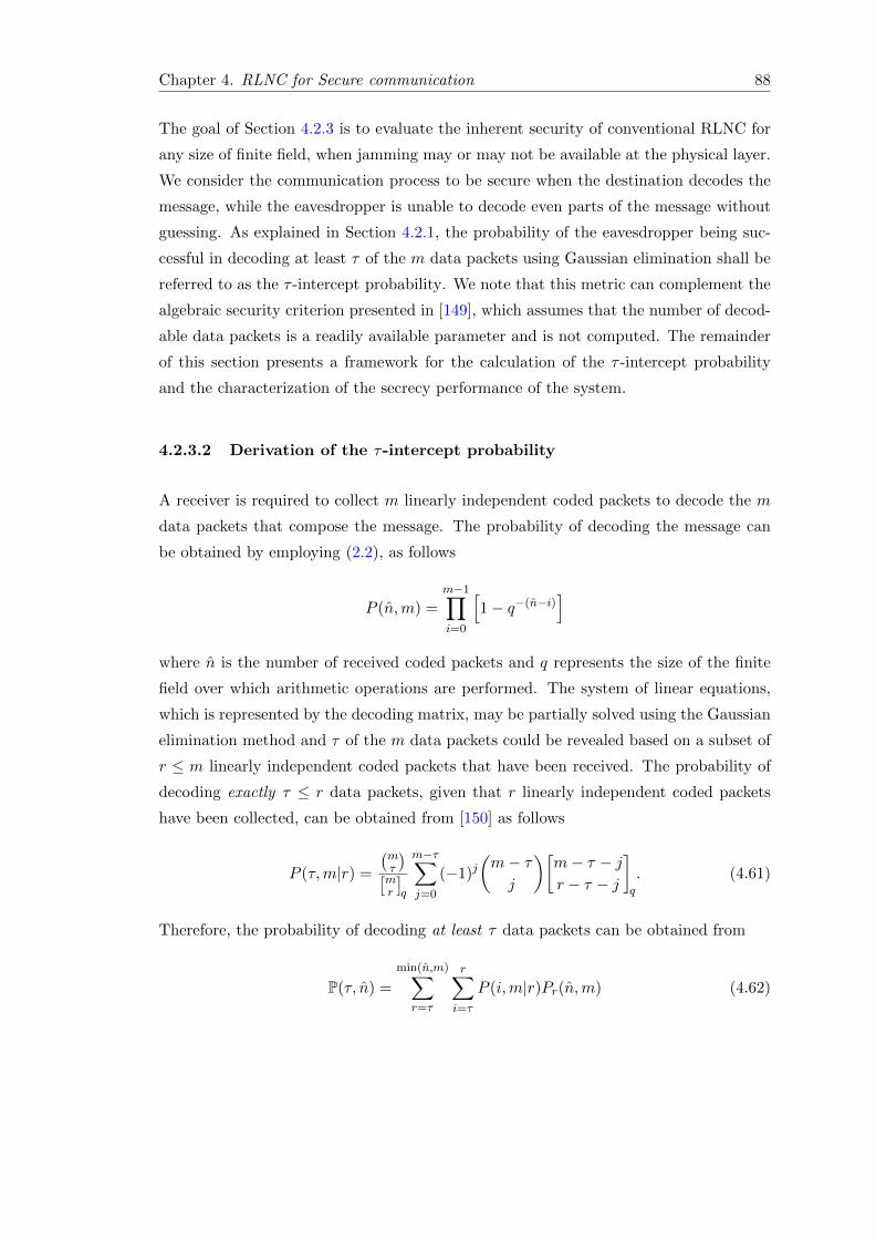
Chapter 4. RLNC for Secure communication 88
The goal of Section 4.2.3 is to evaluate the inherent security of conventional RLNC for
any size of finite field, when jamming may or may not be available at the physical layer.
We consider the communication process to be secure when the destination decodes the
message, while the eavesdropper is unable to decode even parts of the message without
guessing. As explained in Section 4.2.1, the probability of the eavesdropper being suc-
cessful in decoding at least τ of the m data packets using Gaussian elimination shall be
referred to as the τ -intercept probability. We note that this metric can complement the
algebraic security criterion presented in [149], which assumes that the number of decod-
able data packets is a readily available parameter and is not computed. The remainder
of this section presents a framework for the calculation of the τ -intercept probability
and the characterization of the secrecy performance of the system.
4.2.3.2 Derivation of the τ-intercept probability
A receiver is required to collect m linearly independent coded packets to decode the m
data packets that compose the message. The probability of decoding the message can
be obtained by employing (2.2), as follows
P (n,m) =m−1∏i=0
[1− q−(n−i)
]where n is the number of received coded packets and q represents the size of the finite
field over which arithmetic operations are performed. The system of linear equations,
which is represented by the decoding matrix, may be partially solved using the Gaussian
elimination method and τ of the m data packets could be revealed based on a subset of
r ≤ m linearly independent coded packets that have been received. The probability of
decoding exactly τ ≤ r data packets, given that r linearly independent coded packets
have been collected, can be obtained from [150] as follows
P (τ,m|r) =
(mτ
)[mr
]q
m−τ∑j=0
(−1)j(m− τj
)[m− τ − jr − τ − j
]q
. (4.61)
Therefore, the probability of decoding at least τ data packets can be obtained from
P(τ, n) =
min(n,m)∑r=τ
r∑i=τ
P (i,m|r)Pr(n,m) (4.62)
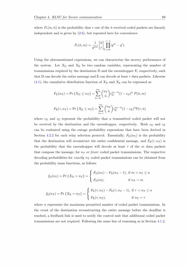
Chapter 4. RLNC for Secure communication 89
where Pr(m, n) is the probability that r out of the n received coded packets are linearly
independent and is given by (2.6), but repeated here for convenience
Pr(n,m) =1
qnm
[n
r
]q
r−1∏i=0
(qm − qi).
Using the aforementioned expressions, we can characterize the secrecy performance of
the system. Let XD and XE be two random variables, representing the number of
transmissions required by the destination D and the eavesdropper E, respectively, such
that D can decode the entire message and E can decode at least τ data packets. Likewise
(4.1), the cumulative distribution function of XD and XE can be expressed as
FD(nT) = Pr {XD ≤ nT} =
nT∑n=m
(nT
n
)εnT−nD (1− εD)n P (n,m)
FE(τ, nT) = Pr {XE ≤ nT} =
nT∑n=τ
(nT
n
)εnT−nE (1− εE)nP(τ, n)
where εD and εE represent the probability that a transmitted coded packet will not
be received by the destination and the eavesdropper, respectively. Both εD and εE
can be evaluated using the outage probability expressions that have been derived in
Section 4.2.2 for each relay selection protocol. Essentially, FD(nT) is the probability
that the destination will reconstruct the entire confidential message, and FE(τ, nT) is
the probability that the eavesdropper will decode at least τ of the m data packets
that compose the message, for nT or fewer coded packet transmissions. The respective
decoding probabilities for exactly nT coded packet transmissions can be obtained from
the probability mass functions, as follows
fD(nT) = Pr {XD = nT} =
FD(nT)− FD(nT − 1), if m < nT ≤ n
FD(m), if nT = m
fE(nT) = Pr {XE = nT} =
FE(τ, nT)− FE(τ, nT − 1), if τ < nT ≤ n
FE(τ, nT), if nT = τ
where n represents the maximum permitted number of coded packet transmissions. In
the event of the destination reconstructing the entire message before the deadline is
reached, a feedback link is used to notify the control unit that additional coded packet
transmissions are not required. Following the same line of reasoning as in Section 4.1.2,
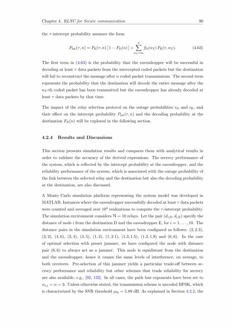
Chapter 4. RLNC for Secure communication 90
the τ -intercept probability assumes the form
Pint(τ, n) = FE(τ, n) [ 1− FD(n) ] +n∑
nT=m
fD(nT)FE(τ, nT). (4.63)
The first term in (4.63) is the probability that the eavesdropper will be successful in
decoding at least τ data packets from the intercepted coded packets but the destination
will fail to reconstruct the message after n coded packet transmissions. The second term
represents the probability that the destination will decode the entire message after the
nT-th coded packet has been transmitted but the eavesdropper has already decoded at
least τ data packets by that time.
The impact of the relay selection protocol on the outage probabilities εD and εE, and
their effect on the intercept probability Pint(τ, n) and the decoding probability at the
destination FD(n) will be explored in the following section.
4.2.4 Results and Discussions
This section presents simulation results and compares them with analytical results in
order to validate the accuracy of the derived expressions. The secrecy performance of
the system, which is reflected by the intercept probability at the eavesdropper, and the
reliability performance of the system, which is associated with the outage probability of
the link between the selected relay and the destination but also the decoding probability
at the destination, are also discussed.
A Monte Carlo simulation platform representing the system model was developed in
MATLAB. Instances where the eavesdropper successfully decoded at least τ data packets
were counted and averaged over 104 realizations to compute the τ -intercept probability.
The simulation environment considers N = 10 relays. Let the pair (di,D, di,E) specify the
distance of node i from the destination D and the eavesdropper E, for i = 1, . . . , 10. The
distance pairs in the simulation environment have been configured as follows: (2, 2.3),
(3, 2), (4, 6), (3, 4), (4, 5), (1, 2), (1, 2.1), (1.3, 1.5), (1.2, 1.9) and (6, 6). In the case
of optimal selection with preset jammer, we have configured the node with distance
pair (6, 6) to always act as a jammer. This node is equidistant from the destination
and the eavesdropper, hence it causes the same levels of interference, on average, to
both receivers. Pre-selection of this jammer yields a particular trade-off between se-
crecy performance and reliability but other schemes that trade reliability for secrecy
are also available, e.g., [92, 132]. In all cases, the path loss exponents have been set to
αi,j = α = 3. Unless otherwise stated, the transmission scheme is uncoded BPSK, which
is characterized by the SNR threshold ρth = 5.89 dB. As explained in Section 4.2.2, the
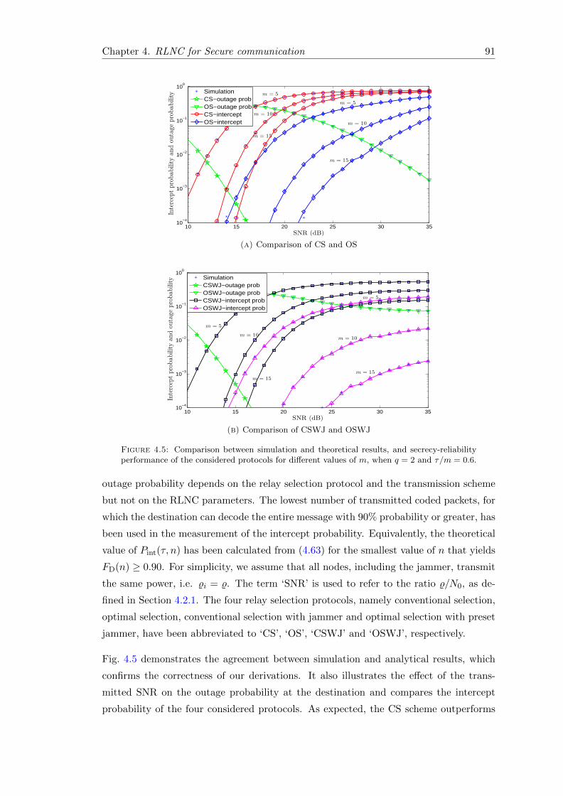
Chapter 4. RLNC for Secure communication 91
10 15 20 25 30 3510
−4
10−3
10−2
10−1
100
SNR (dB)
Intercep
tprobab
ility
andou
tage
probab
ility
SimulationCS−outage probOS−outage probCS−interceptOS−intercept
m = 5
m = 10
m = 15
m = 5
m = 10
m = 15
(a) Comparison of CS and OS
10 15 20 25 30 3510
−4
10−3
10−2
10−1
100
SNR (dB)
Intercep
tprobab
ility
andou
tage
probab
ility
SimulationCSWJ−outage probOSWJ−outage probCSWJ−intercept probOSWJ−intercept prob
m = 5
m = 10
m = 15
m = 5
m = 10
m = 15
(b) Comparison of CSWJ and OSWJ
Figure 4.5: Comparison between simulation and theoretical results, and secrecy-reliabilityperformance of the considered protocols for different values of m, when q = 2 and τ/m = 0.6.
outage probability depends on the relay selection protocol and the transmission scheme
but not on the RLNC parameters. The lowest number of transmitted coded packets, for
which the destination can decode the entire message with 90% probability or greater, has
been used in the measurement of the intercept probability. Equivalently, the theoretical
value of Pint(τ, n) has been calculated from (4.63) for the smallest value of n that yields
FD(n) ≥ 0.90. For simplicity, we assume that all nodes, including the jammer, transmit
the same power, i.e. %i = %. The term ‘SNR’ is used to refer to the ratio %/N0, as de-
fined in Section 4.2.1. The four relay selection protocols, namely conventional selection,
optimal selection, conventional selection with jammer and optimal selection with preset
jammer, have been abbreviated to ‘CS’, ‘OS’, ‘CSWJ’ and ‘OSWJ’, respectively.
Fig. 4.5 demonstrates the agreement between simulation and analytical results, which
confirms the correctness of our derivations. It also illustrates the effect of the trans-
mitted SNR on the outage probability at the destination and compares the intercept
probability of the four considered protocols. As expected, the CS scheme outperforms

Chapter 4. RLNC for Secure communication 92
10 15 20 25 30 3510
−10
10−8
10−6
10−4
10−2
100
SNR (dB)
Intercep
tprobability
CSWJ (q = 2)
CSWJ (q = 4)
OSWJ (q = 2)
OSWJ (q = 4)
Figure 4.6: Effect of the field size q on the secrecy performance of both CSWJ and OSWJ,as a function of the SNR, when τ = 8 and m = 15.
the other protocols in terms of reliable communication because it achieves the lowest
outage probability. By contract, the CS protocol exhibits the worst performance in
terms of secrecy. This is due to the fact that the CS protocol only considers the quality
of relay-to-destination channels but does not take into account the relay-to-eavesdropper
channels. For this reason, the OS and CSWJ protocols offer better secrecy performance
than CS at the expense of reduced reliability. It can be noticed that the secrecy per-
formance of both the CS and OS protocols deteriorates markedly at high SNR values
because the intercept probability converges to one. On the other hand, the secrecy per-
formance of the CSWJ and OSWJ protocols reveals that a jammer introduces a ‘ceiling’
to the intercept probability and, thus, a level of secrecy can be offered even at high SNR
values. Fig. 4.5 also demonstrates that the secrecy-reliability tradeoff can be further
improved if the message to be transmitted is segmented into a larger number of shorter
data packets, that is, the value of m in RLNC is increased.
Fig. 4.6 investigates the effect that the field size q in RLNC has on the probability that
the eavesdropper will reconstruct at least τ = 8 data packets from the intercepted coded
packets, for different SNR values, when m = 15 and either CSWJ or OSWJ is used.
The figure shows that when the field size increases from q = 2 to q = 4, the intercept
probability decreases notably. This is due to the fact that the larger the finite field is,
the higher the probability of the received coded packets being linearly independent is.
Consequently, if q = 4, the destination is required to collect fewer coded packets in order
to reconstruct the entire message than if q = 2. On the other hand, if the finite field is
large and the rank of the decoding matrix is smaller than m, the probability of partially
reconstructing the transmitted message reduces significantly. For this reason, the fewer
the linearly independent coded packets intercepted by the eavesdropper are, the smaller
the probability of the eavesdropper decoding even a fraction of the message is. Fig. 4.5
and Fig. 4.6 reveal the impact of the number of data packets m and the field size q on
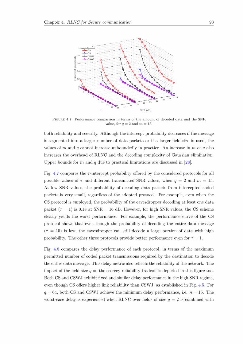
Chapter 4. RLNC for Secure communication 93
13
57
911
1315 16
1718
1920
2122
2324
25
0
0.2
0.4
0.6
0.8
1
SNR (dB)τ
τ-interceptprobability
CSOSCSWJOSWJ
Figure 4.7: Performance comparison in terms of the amount of decoded data and the SNRvalue, for q = 2 and m = 15.
both reliability and security. Although the intercept probability decreases if the message
is segmented into a larger number of data packets or if a larger field size is used, the
values of m and q cannot increase unboundedly in practice. An increase in m or q also
increases the overhead of RLNC and the decoding complexity of Gaussian elimination.
Upper bounds for m and q due to practical limitations are discussed in [28].
Fig. 4.7 compares the τ -intercept probability offered by the considered protocols for all
possible values of τ and different transmitted SNR values, when q = 2 and m = 15.
At low SNR values, the probability of decoding data packets from intercepted coded
packets is very small, regardless of the adopted protocol. For example, even when the
CS protocol is employed, the probability of the eavesdropper decoding at least one data
packet (τ = 1) is 0.18 at SNR = 16 dB. However, for high SNR values, the CS scheme
clearly yields the worst performance. For example, the performance curve of the CS
protocol shows that even though the probability of decoding the entire data message
(τ = 15) is low, the eavesdropper can still decode a large portion of data with high
probability. The other three protocols provide better performance even for τ = 1.
Fig. 4.8 compares the delay performance of each protocol, in terms of the maximum
permitted number of coded packet transmissions required by the destination to decode
the entire data message. This delay metric also reflects the reliability of the network. The
impact of the field size q on the secrecy-reliability tradeoff is depicted in this figure too.
Both CS and CSWJ exhibit fixed and similar delay performance in the high SNR regime,
even though CS offers higher link reliability than CSWJ, as established in Fig. 4.5. For
q = 64, both CS and CSWJ achieve the minimum delay performance, i.e. n = 15. The
worst-case delay is experienced when RLNC over fields of size q = 2 is combined with
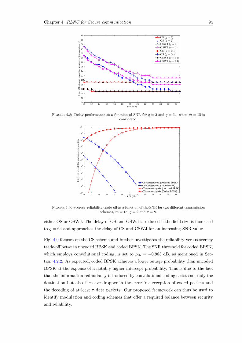
Chapter 4. RLNC for Secure communication 94
10 12 14 16 18 20 22 24 26 28 30 32 3410
12
14
16
18
20
22
24
26
28
30
32
34
36
38
40
SNR (dB)
Delay(M
axim
um
permittednumber
oftransm
issionsn)
CS (q = 2)
OS (q = 2)
CSWJ (q = 2)
OSWJ (q = 2)
CS (q = 64)
OS (q = 64)
CSWJ (q = 64)
OSWJ (q = 64)
Figure 4.8: Delay performance as a function of SNR for q = 2 and q = 64, when m = 15 isconsidered.
10 12 14 16 18 20 22 24 26 28 30 32 3410
−10
10−9
10−8
10−7
10−6
10−5
10−4
10−3
10−2
10−1
100
SNR (dB)
Interceptprobab
ilityan
dou
tage
probab
ility
CS−outage prob. (Uncoded BPSK)CS−outage prob. (Coded BPSK)CS−intercept prob. (Uncoded BPSK)CS−intercept prob. (Coded BPSK)
Figure 4.9: Secrecy-reliability trade-off as a function of the SNR for two different transmissionschemes, m = 15, q = 2 and τ = 8.
either OS or OSWJ. The delay of OS and OSWJ is reduced if the field size is increased
to q = 64 and approaches the delay of CS and CSWJ for an increasing SNR value.
Fig. 4.9 focuses on the CS scheme and further investigates the reliability versus secrecy
trade-off between uncoded BPSK and coded BPSK. The SNR threshold for coded BPSK,
which employs convolutional coding, is set to ρth = −0.983 dB, as mentioned in Sec-
tion 4.2.2. As expected, coded BPSK achieves a lower outage probability than uncoded
BPSK at the expense of a notably higher intercept probability. This is due to the fact
that the information redundancy introduced by convolutional coding assists not only the
destination but also the eavesdropper in the error-free reception of coded packets and
the decoding of at least τ data packets. Our proposed framework can thus be used to
identify modulation and coding schemes that offer a required balance between security
and reliability.
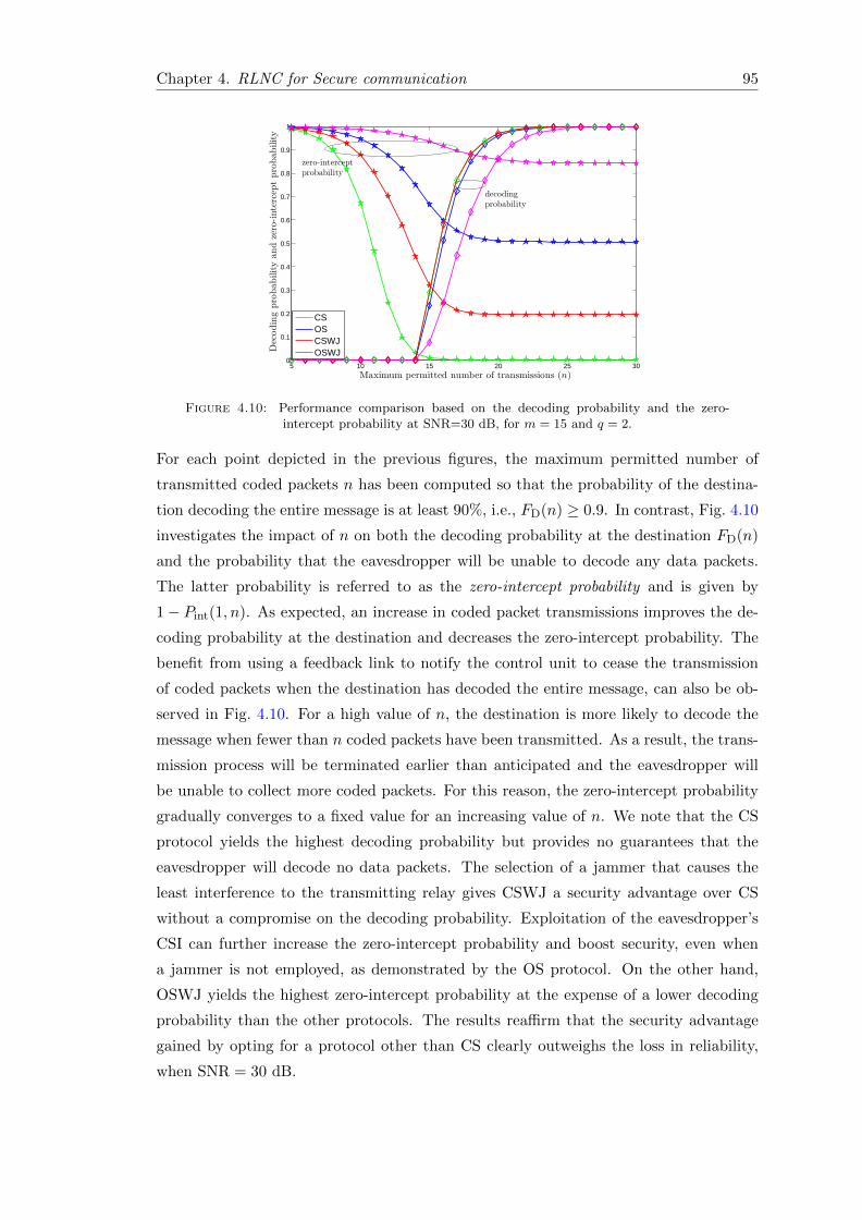
Chapter 4. RLNC for Secure communication 95
5 10 15 20 25 300
0.1
0.2
0.3
0.4
0.5
0.6
0.7
0.8
0.9
1
Maximum permitted number of transmissions (n)
Decodingprobabilityandzero-intercep
tprobability
CSOSCSWJOSWJ
decodingprobability
zero-interceptprobability
Figure 4.10: Performance comparison based on the decoding probability and the zero-intercept probability at SNR=30 dB, for m = 15 and q = 2.
For each point depicted in the previous figures, the maximum permitted number of
transmitted coded packets n has been computed so that the probability of the destina-
tion decoding the entire message is at least 90%, i.e., FD(n) ≥ 0.9. In contrast, Fig. 4.10
investigates the impact of n on both the decoding probability at the destination FD(n)
and the probability that the eavesdropper will be unable to decode any data packets.
The latter probability is referred to as the zero-intercept probability and is given by
1− Pint(1, n). As expected, an increase in coded packet transmissions improves the de-
coding probability at the destination and decreases the zero-intercept probability. The
benefit from using a feedback link to notify the control unit to cease the transmission
of coded packets when the destination has decoded the entire message, can also be ob-
served in Fig. 4.10. For a high value of n, the destination is more likely to decode the
message when fewer than n coded packets have been transmitted. As a result, the trans-
mission process will be terminated earlier than anticipated and the eavesdropper will
be unable to collect more coded packets. For this reason, the zero-intercept probability
gradually converges to a fixed value for an increasing value of n. We note that the CS
protocol yields the highest decoding probability but provides no guarantees that the
eavesdropper will decode no data packets. The selection of a jammer that causes the
least interference to the transmitting relay gives CSWJ a security advantage over CS
without a compromise on the decoding probability. Exploitation of the eavesdropper’s
CSI can further increase the zero-intercept probability and boost security, even when
a jammer is not employed, as demonstrated by the OS protocol. On the other hand,
OSWJ yields the highest zero-intercept probability at the expense of a lower decoding
probability than the other protocols. The results reaffirm that the security advantage
gained by opting for a protocol other than CS clearly outweighs the loss in reliability,
when SNR = 30 dB.
Chapter 4. RLNC for Secure communication 96
4.3 Summary
The main contributions made in this chapter can be summarized as follows:
• In Section 4.1, we derived accurate expressions for the intercept probability of
a network, where a transmitter uses random linear network coding to broadcast
information. Both unaided transmission and feedback-aided transmission were in-
vestigated and the secrecy gain achieved by the latter approach was computed.
Moreover, we presented a resource allocation model to minimize the intercept
probability, while satisfying delay and reliability constraints, and showed that the
legitimate receiver is not required to have knowledge of the presence of an eaves-
dropper.
• In Secction 4.2, we proposed a cross-layer security scheme, which combines the
inherent secrecy features of RLNC at the application layer with physical-layer
security mechanisms, based on relay selection with or without jamming. We de-
rived analytical expressions of the outage probability at the destination and the
eavesdropper. We introduced a novel secrecy metric, which is referred to as the
τ−intercept probability and is defined as the probability that a proportion of
the transmitted information will be compromised. An exact expression of the τ -
intercept probability is derived for systems that impose a deadline on coded packet
transmissions but provide the destination with a feedback link, which can be used
to terminate the transmission process before the deadline expires. Furthermore,
we investigated the secrecy-reliability trade-offs of the considered RLNC-enabled
relay selection protocols.
Chapter 5
Conclusions and Future Research
Directions
In Chapters 2 to 4, we have studied several performance aspects of RLNC. In this
chapter, we present general conclusions drawn from each chapter of this thesis. More
detailed technical contributions can be found at the end of each chapter and are not
repeated here. Finally, we also exhibit some possible future directions emerging from
this work.
5.1 Summary and Conclusions of the Thesis
In Chapter 2, closed form analytical expressions have been derived to evaluate and char-
acterize the performance of non-overlapping, expanding and sliding generations RLNC
schemes. These schemes support point-to-point and point-to-multipoint communica-
tions, and are practically useful to exploit the sparsity and prioritization features of
RLNC in order to provide unequal error protection and reduced decoding complexity.
Moreover, the design parameters of these schemes allow to adjust the desired decoding
performance. For instance, the derived expressions for RLNC using sliding generations
that can overlap by up to 50% demonstrated that a low amount of overlap between gen-
erations in practical settings can yield a similar decoding probability to that of the more
computationally expensive RLNC based on expanding generations. We note that if the
system parameters impose an overlap bigger than 50% between generations, (e.g., when
the field size is small, the number of source packets is high and the channel conditions
are poor) the expressions of the decoding probability of expanding-generations RLNC
and sliding-generations RLNC can be used as upper and lower bounds, respectively.
97
Chapter 5. Conclusions 98
In Chapter 3, we primarily focused on the development of mathematical frameworks to
evaluate and characterise the performance of RLNCC. In this respect, we first formu-
lated the performance of single relay networks combining intra-session and inter-session
RLNC. It has been shown that, depending on the channel qualities, systematic RLNC
can provide equivalent or better decoding performance than non-systematic RLNC. Sec-
ondly, theoretical closed form expressions were derived to evaluate the performance of
RLNC in multi-source multi-relay networks. We exhibited that the proposed frame-
work can be employed to characterize the performance of opportunistic as well as sparse
RLNC. Finally, we have proposed the use of RLNCC combined with NOMA for uplink
multi-source multi-relay networks. In this work, we have demonstrated the gains in
terms of decoding probability, diversity and throughput performance in comparison to
conventional OMA based RLNCC.
In Chapter 4, we presented RLNC as a self encryption technique for secure communica-
tions. In this respect, we have formulated and characterized the inherent secrecy feature
of RLNC, and demonstrated the importance of feedback based controlled transmissions
and the finite field effect on network security. Moreover, we proposed a framework that
combines RLNC at the application layer and physical-layer security in the form of relay
selection with or without cooperative jamming. Four relay selection protocols were con-
sidered and analytical expressions of the outage probability at the intended destination
and the eavesdropper were derived. In order to quantify the amount of information leak-
age to the eavesdropper, a novel metric called τ -intercept probability was proposed. This
metric, which utilizes the outage probabilities associated to each relay selection protocol,
characterizes the security that is jointly offered by the application and physical layers.
Our analysis demonstrated that relay selection based on both the eavesdropper’s CSI
and the destination’s CSI achieves a good balance between security and reliability, when
a jammer is not employed. If a jammer is used, reliability can be traded for security. On
the other hand, if the eavesdropper’s CSI is not available, the selection of a relay and a
jammer based solely on the destination’s CSI favors reliability, while still providing some
secrecy guarantees. We also noted that the field size over which RLNC is performed
at the application layer as well as the adopted modulation and coding scheme at the
physical layer can be modified to fine-tune the trade-off between security and reliability.
5.2 Future Directions
The following are proposed research directions that could be investigated as an extension
to the research presented in this thesis.

Chapter 5. Conclusions 99
• Distributed Memory management and heterogeneous IoT devises: The
analysis and the work presented in Chapter 2 could be extended to design dis-
tributed storage schemes, and communication schemes to support heterogeneous
IoT devices with different computation power.
• Energy harvesting and software defined network environment: The re-
search work presented in Chapter 3 could be extended to design NOMA-RLNCC
based energy harvesting techniques for green content delivery. Moreover, the ad-
vantages of RLNCC could be exploited in software defined network environment for
data managements and low power receivers of limited computational capabilities.
• Joint user pairing and RLNCC: The research work presented in Chapter 4 can
be extended by designing a joint user pairing and RLNCC scheme for improving
the security and reliability performance of NOMA based communications.
Appendix A
Analytical proof of Lemma 2.1
The objective of this Appendix is to analytically prove that
∑r1
γr1(n1,m) γ(n2,m−r1)qn2r1 = γ(n1 + n2, m) (A.1)
for max(0,m−n2) ≤ r1 ≤ min(n1,m), and thus show that (2.1) and (2.7) are equivalent
expressions. If we both divide and multiply the left-hand side of (A.1) by γ(m,m) and
use (2.3) and (2.5) to expand γr1(n1,m) and γ(n2,m− r1), respectively, we obtain
∑r1
γr1(n1,m)γ(n2,m− r1)qn2r1 =γ(m,m)∑r1
[n1
r1
]q
[n2
m− r1
]q
γ(m, r1) γ(m−r1,m−r1)
γ(m,m)qn2r1 . (A.2)
Expression (2.1) can be used to compute the ratio of the γ functions in the sum of (C.1)
as follows
γ(m, r1) γ(m−r1,m−r1)
γ(m,m)=
∏m−r1−1i=0 (qm−r1 − qi)∏m−1
i=r1(qm − qi)
= q−r1(m−r1). (A.3)
If we substitute (C.2) into (C.1) and invoke the following identity
∑r1
[n1
r1
]q
[n2
m− r1
]q
qr1(n2−m+r1) =
[n1 + n2
m
]q
(A.4)
which is known as the q-Vandermonde identity, expression (C.1) reduces to
∑r1
γr1(n1,m)γ(n2,m− r1)qn2r1 =γ(m,m)
[n1+n2
m
]q
. (A.5)
The right-hand side of (C.3) is equal to γ(n1+n2,m) as per (2.5), which completes the
proof.
100
Appendix B
Reformulation of the intercept
probability of FT
Based on the definition of the PMF in (4.2), the expression for PBE(n) in (4.4) can be
expanded as follows:
PBE(n) = FB(m)FE(m)− FB(m)FE(m+ 1) + FB(m+ 1)FE(m+ 1)
− FB(n− 1)FE(n) + FB(n)FE(n).
If we create pairs from each two consecutive terms, with the exception of the last term,
and invoke again the definition of the PMF, we obtain
PBE(n) =
[−
n∑nT=m+1
fE(nT)FB(nT − 1)
]+ FB(n)FE(n).
In (4.5), we established that PE(n) = FE(n) − FB(n)FE(n). Using (4.3), the intercept
probability of FT can be expressed as:
P FTint (n) = FE(n)−
n∑nT=m+1
fE(nT)FB(nT − 1). (B.1)
101
Appendix C
Proof of Proposition 4.2 for the
case of FT
In order to prove Proposition 4.2 for the FT mode, it suffices to set ∆ = Pint(n2) −Pint(n1) and show that ∆ ≥ 0 for all n2 ≥ n1. Using (B.1), we find that
∆ = FE(n2)− FE(n1)−n2∑
nT=n1+1
fE(nT)FB(nT − 1). (C.1)
Terms −FE(i) and FE(i) for i = n1 + 1, . . . , n2 − 1, which cancel each other out, are
added to FE(n2)− FE(n1) and give
FE(n2)− FE(n1) = (FE(n2)− FE(n2 − 1)) + . . .
. . .+ (FE(n1 + 1)− FE(n1))
=
n2∑nT=n1+1
fE(nT).
(C.2)
If we substitute (C.2) into (C.1), we obtain
∆ =
n2∑nT=n1+1
fE(nT)[1− FB(nT − 1)
]which is a sum of non-negative terms and is, thus, ∆ ≥ 0.
102
Bibliography
[1] R. Ahlswede, N. Cai, S.-Y. R. Li, and R. W. Yeung, “Network information flow,”
IEEE Trans. Inf. Theory, vol. 46, no. 4, pp. 1204–1216, Jul. 2000.
[2] E. Ahmed, A. Eryilmaz, M. Medard, and A. E. Ozdaglar, “On the scaling law of
network coding gains in wireless networks,” in Proc. IEEE Military Communica-
tions Conference, Orlando, FL, USA, Oct. 2007.
[3] J. sang Park, M. Gerla, D. S. Lun, Y. yi, and M. Medard, “Codecast: a network-
coding-based ad hoc multicast protocol,” IEEE Wireless Communications, vol. 13,
no. 5, pp. 76–81, Oct. 2006.
[4] M. Ghaderi, D. Towsley, and J. Kurose, “Reliability gain of network coding in
lossy wireless networks,” in Proc. IEEE Conference on Computer Communications
(INFOCOM), Phoenix, AZ, USA, Apr. 2008.
[5] J. Zhang, P. Fan, and K. B. Letaief, “Network coding for efficient multicast routing
in wireless ad-hoc networks,” IEEE Trans. Commun., vol. 56, no. 4, pp. 598–607,
Apr. 2008.
[6] T. Ho, M. Medard, R. Koetter, D. R. Karger, M. Effros, J. Shi, and B. Leong, “A
random linear network coding approach to multicast,” IEEE Trans. Inf. Theory,
vol. 52, no. 10, pp. 4413–4430, Oct. 2006.
[7] Y. Chen, S. Kishore, and J. Li, “Wireless diversity through network coding,” in
IEEE Wireless Communications and Networking Conference, Las Vegas, USA,
Apr. 2006.
[8] R. Bassoli, H. Marques, J. Rodriguez, K. W. Shum, and R. Tafazolli, “Network
coding theory: A survey,” IEEE Commun. Surveys Tuts., vol. 15, no. 4, pp. 1950–
1978, Fourth Quarter 2013.
[9] Y. Yang, C. Zhong, Y. Sun, and J. Yang, “Energy efficient reliable multi-path
routing using network coding for sensor network,” Int. Journal of Comp. Science
and Net. Sec., vol. 8, no. 12, pp. 329–338, Dec. 2008.
103
Chapter 5. Conclusions 104
[10] X. Wang, Y. Xu, and Z. Feng, “Physical-layer network coding in OFDM system:
Analysis and performance,” in International Conference on Communications and
Networking, Kunming, China, Aug. 2012.
[11] S. T. Basaran, G. K. Kurt, M. Uysal, and I. Altunbas, “A tutorial on network
coded cooperation,” IEEE Commun. Surveys Tuts., vol. 18, no. 4, pp. 2970–2990,
Fourthquarter 2016.
[12] S. Gokceli, H. Alakoca, S. T. Basaran, and G. K. Kurt, “OFDMA-based network-
coded cooperation: design and implementation using software-defined radio
nodes,” EURASIP Journal on Advances in Signal Processing, vol. 2016, no. 1,
p. 8, Jan. 2016.
[13] Z. Ding, Z. Yang, P. Fan, and H. V. Poor, “On the performance of non-orthogonal
multiple access in 5G systems with randomly deployed users,” IEEE Signal Pro-
cess. Lett., vol. 21, no. 12, pp. 1501–1505, Dec. 2014.
[14] S. Timotheou and I. Krikidis, “Fairness for non-orthogonal multiple access in 5G
systems,” IEEE Signal Process. Lett., vol. 22, no. 10, pp. 1647–1651, Oct. 2015.
[15] X. Li, C. Li, and Y. Jin, “Dynamic resource allocation for transmit power mini-
mization in OFDM-based NOMA systems,” IEEE Commun. Lett., vol. 20, no. 12,
pp. 2558–2561, Dec. 2016.
[16] P. Parida and S. S. Das, “Power allocation in OFDM based NOMA systems: A
DC programming approach,” in Proc. IEEE Globecom Workshops (GC Wkshps),
Texas, USA, Dec. 2014.
[17] S. Park and D.-H. Cho, “Random linear network coding based on non-orthogonal
multiple access in wireless networks,” IEEE Commun. Lett., vol. 19, no. 7, pp.
1273–1276, Jul. 2015.
[18] H. Seferoglu, A. Markopoulou, and K. K. Ramakrishnan, “I2NC: Intra- and inter-
session network coding for unicast flows in wireless networks,” in Proc. IEEE
Conference on Computer Communications (INFOCOM), Shanghai, China, Apr.
2011.
[19] W. Chen, K. B. Letaief, and Z. Cao, “Opportunistic network coding for wireless
networks,” in Proc. IEEE Intern. Conf. on Commun. (ICC), Glasgow, UK, Jun.
2007.
[20] H. Seferoglu and A. Markopoulou, “Opportunistic network coding for video
streaming over wireless,” in Packet Video. Lausanne, Switzerland: IEEE, Nov.
2007.
Chapter 5. Conclusions 105
[21] M. Wang and B. Li, “Lava: A reality check of network coding in peer-to-peer
live streaming,” in IEEE International Conference on Computer Communications
(INFOCOM), Barcelona, Spain, May 2007.
[22] J. M. Walsh and S. Weber, “A concatenated network coding scheme for multime-
dia transmission,” in Network Coding, Theory and Applications ( NetCod), Hong
Kong, China, Jan. 2008.
[23] M. Wang and B. Li, “Network coding in live peer-to-peer streaming,” IEEE Trans-
actions on Multimedia, vol. 9, no. 8, pp. 1554–1567, 2007.
[24] S. Zhang, S. C. Liew, and P. P. Lam, “Hot topic: Physical-layer network coding,”
in International conference on Mobile computing and networking (MobiCom), Los
Angeles, California, Sep. 2006.
[25] S. C. Liew, S. Zhang, and L. Lu, “Physical-layer network coding: Tutorial, survey,
and beyond,” Physical Communication, vol. 6, pp. 4–42, 2013.
[26] S. Deb, M. Effros, T. Ho, D. R. Karger, R. Koetter, D. S. Lun, M. Medard, and
N. Ratnakar, “Network coding for wireless applications: A brief tutorial,” in Proc.
Int. Workshop on Wireless Ad Hoc Networks, London, UK, May 2005.
[27] D. Szabo, A. Gulyas, F. H. P. Fitzek, and D. E. Lucani, “Towards the tactile
internet: Decreasing communication latency with network coding and software
defined networking,” in Proc. European Wireless Conf., Budapest, Hungary, May
2015.
[28] J. Heide, M. V. Pedersen, F. H. Fitzek, and M. Medard, “On code parameters and
coding vector representation for practical RLNC,” in Proc. IEEE Intern. Conf. on
Commun. (ICC), Kyoto, Japan, Jun. 2011.
[29] C. W. Sørensen, D. E. Lucani, F. H. P. Fitzek, and M. Medard, “On-the-fly
overlapping of sparse generations: A tunable sparse network coding perspective,”
in Proc. IEEE Veh. Tech. Conf. (VTC Fall), Vancouver, BC, Sep. 2014.
[30] P. Maymounkov, N. J. A. Harvey, and D. S. Lun, “Methods for efficient network
coding,” in Proc. Allerton Conf. on Commun., Control and Comp, Monticello, IL,
USA, Sep. 2006.
[31] D. Vukobratovic and V. Stankovic, “Unequal error protection random linear coding
strategies for erasure channels,” IEEE Trans. Commun., vol. 60, no. 5, pp. 1243–
1252, May 2012.
Chapter 5. Conclusions 106
[32] Y. Li, E. Soljanin, and P. Spasojevic, “Effects of the generation size and overlap on
throughput and complexity in randomized linear network coding,” IEEE Trans.
Inf. Theory, vol. 57, no. 2, pp. 1111–1123, Feb. 2011.
[33] A. Heidarzadeh and A. H. Banihashemi, “Overlapped chunked network coding,”
in Proc. IEEE Inform. Theory Workshop (ITW), Cairo, Egypt, Jan. 2010.
[34] M. C. Bogino, P. Cataldi, M. Grangetto, E. Magli, and G. Olmo, “Sliding-window
digital fountain codes for streaming of multimedia contents,” in Proc. IEEE Int.
Symp. on Circ. and Systems (ISCAS), New Orleans, LA, May 2007.
[35] Y. Lin, B. Liang, and B. Li, “SlideOR: Online opportunistic network coding in
wireless mesh networks,” in Proc. IEEE Conference on Computer Communications
(INFOCOM), San Diego, CA, Mar. 2010.
[36] D. J. C. MacKay, “Fountain codes,” IEE Proc.-Communications, vol. 152, no. 6,
pp. 1062–1068, Dec. 2005.
[37] S. Feizi, D. E. Lucani, and M. Medard, “Tunable sparse network coding,” in Proc.
Int. Zurich Seminar on Commun. (IZS), Zurich, Switzerland, Feb. 2012.
[38] X. Chu, K. Zhao, and M. Wang, “Practical random linear network coding on
GPUs,” NETWORKING, pp. 573–585, 2009.
[39] F. H. Fitzek, M. V. Pedersen, J. Heide, and M. Medard, “Network coding: ap-
plications and implementations on mobile devices,” in Proc. ACM workshop on
Performance monitoring and measurement of heterogeneous wireless and wired
networks, 2010, pp. 83–87.
[40] G. Angelopoulos, A. Paidimarri, A. P. Chandrakasan, and M. Medard, “Experi-
mental study of the interplay of channel and network coding in low power sensor
applications,” in Proc. IEEE Intern. Conf. on Commun. (ICC), Budapest, Hun-
gary, Jun. 2013.
[41] C. Khirallah, D. Vukobratovic, and J. Thompson, “Performance analysis and en-
ergy efficiency of random network coding in lte-advanced,” IEEE Trans. Wireless
Commun., vol. 11, no. 12, pp. 4275–4285, Dec. 2012.
[42] K. Nguyen, T. Nguyen, and S.-C. Cheung, “Video streaming with network coding,”
Journal of Signal Processing Systems, vol. 59, no. 3, pp. 319–333, 2010.
[43] A. Tassi, I. Chatzigeorgiou, and D. Vukobratovic, “Resource-allocation frame-
works for network-coded layered multimedia multicast services,” IEEE J. Sel.
Areas Commun., vol. 33, no. 2, pp. 141–155, Feb. 2015.
Chapter 5. Conclusions 107
[44] M. Esmaeilzadeh, P. Sadeghi, and N. Aboutorab, “Random linear network cod-
ing for wireless layered video broadcast: General design methods for adaptive
feedback-free transmission,” IEEE Trans. Commun., pp. 790–805, Feb. 2017.
[45] N. J. H. Marcano, J. Heide, D. E. Lucani, and F. H. P. Fitzek, “On the over-
head of telescopic codes in network coded cooperation,” in Proc. IEEE Vehicular
Technology Conference (VTC), Boston, USA, Sep. 2015.
[46] C. Gkantsidis and P. R. Rodriguez, “Network coding for large scale content distri-
bution,” in Proc. Joint Conference of the IEEE Computer and Communications
Societies., Miami, FL, USA, Mar. 2005.
[47] C. Fragouli and A. Markopoulou, “A network coding approach to overlay network
monitoring,” in Proc. Allerton Conf. on Commun., Control and Comp, Illinois,
USA, Sep. 2005.
[48] T. Ho, B. Leong, Y.-H. Chang, Y. Wen, and R. Koetter, “Network monitoring in
multicast networks using network coding,” in Proc. IEEE International Sympo-
sium on Information Theory ( ISIT ), Adelaide, Australia, Sep. 2005.
[49] W. Guo, X. Shi, N. Cai, and M. Medard, “Localized dimension growth: a con-
volutional random network coding approach to managing memory and decoding
delay,” IEEE Trans. Commun., vol. 61, no. 9, pp. 3894–3905, 2013.
[50] S. Moriam, Y. Yan, E. Fischer, E. Franz, and G. P. Fettweis, “Resilient and
efficient communication in many-core systems using network coding,” in Proc. In-
ternational Performance Computing and Communications Conference (IPCCC),
California, USA, Dec. 2015.
[51] D. Platz, D. H. Woldegebreal, and H. Karl, “Random network coding in wireless
sensor networks: Energy efficiency via cross-layer approach,” in Proc. International
Symposium on Spread Spectrum Techniques and Applications, Bologna, Italy, Aug.
2008.
[52] L. Sun, P. Ren, Q. Du, and Y. Wang, “Fountain-coding aided strategy for secure
cooperative transmission in industrial wireless sensor networks,” IEEE Trans. Ind.
Informat., vol. 12, no. 1, pp. 291–300, Feb. 2016.
[53] Y. Lin, B. Liang, and B. Li, “Priority random linear codes in distributed storage
systems,” IEEE Trans. Parallel Distrib. Syst., vol. 20, no. 11, pp. 1653–1667, Nov.
2009.
[54] N. Thomos, E. Kurdoglu, P. Frossard, and M. van der Schaar, “Adaptive priori-
tized random linear coding and scheduling for layered data delivery from multiple
servers,” IEEE Trans. Multimedia, vol. 17, no. 6, pp. 893–906, Jun. 2015.
Chapter 5. Conclusions 108
[55] A. S. Lalos, A. Antonopoulos, E. Kartsakli, M. Di Renzo, S. Tennina, L. Alonso,
and C. Verikoukis, “RLNC-aided cooperative compressed sensing for energy effi-
cient vital signal telemonitoring,” IEEE Trans. Wireless Commun., vol. 14, no. 7,
pp. 3685–3699, 2015.
[56] A. Nasri, R. Schober, and M. Uysal, “Performance and optimization of network-
coded cooperative diversity systems,” IEEE Trans. Commun., vol. 61, no. 3, pp.
1111–1122, 2013.
[57] T. Lv, S. Li, and W. Geng, “Combining cooperative diversity and network cod-
ing in uplink multi-source multi-relay networks,” EURASIP Journal on Wireless
Communications and Networking, vol. 2013, no. 1, p. 241, Dec. 2013.
[58] H. Topakkaya and Z. Wang, “Wireless network code design and performance anal-
ysis using diversity-multiplexing tradeoff,” IEEE Trans. Commun., vol. 59, no. 2,
pp. 488–496, Feb. 2011.
[59] J.-T. Seong, “Bounds on decoding failure probability in linear network coding
schemes with erasure channels,” IEEE Commun. Lett., vol. 18, no. 4, pp. 648–651,
Apr. 2014.
[60] J.-T. Seong and H.-N. Lee, “Predicting the performance of cooperative wire-
less networking schemes with random network coding,” IEEE Trans. Commun.,
vol. 62, no. 8, pp. 2951–2964, Aug. 2014.
[61] N. Cai and R. W. Yeung, “Secure network coding,” in Proc. IEEE Int. Symp. on
Inform. Theory (ISIT), Lausanne, Switzerland, Jun. 2002.
[62] X. Wang, W. Guo, Y. Yang, and B. Wang, “A secure broadcasting scheme with
network coding,” IEEE Commun. Lett., vol. 17, no. 7, pp. 1435–1438, Jul. 2013.
[63] M. Adeli and H. Liu, “On the inherent security of linear network coding,” IEEE
Commun. Lett., vol. 17, no. 8, pp. 1668–1671, Aug. 2013.
[64] H. Niu, M. Iwai, K. Sezaki, L. Sun, and Q. Du, “Exploiting fountain codes for
secure wireless delivery,” IEEE Commun. Lett., vol. 18, no. 5, pp. 777–780, May
2014.
[65] V. C. Gungor and G. P. Hancke, “Industrial wireless sensor networks: Challenges,
design principles, and technical approaches,” IEEE Trans. Ind. Electron., vol. 56,
no. 10, pp. 4258–4265, Oct. 2009.
[66] W. Jiang, T. Kaiser, and A. J. H. Vinck, “A robust opportunistic relaying strat-
egy for co-operative wireless communications,” IEEE Trans. Wireless Commun.,
vol. 15, no. 4, pp. 2642–2655, Apr. 2016.
Chapter 5. Conclusions 109
[67] A. Bletsas, A. Khisti, D. P. Reed, and A. Lippman, “A simple cooperative diversity
method based on network path selection,” IEEE J. Sel. Areas Commun., vol. 24,
no. 3, pp. 659–672, Mar. 2006.
[68] J. Luo, J. Hu, D. Wu, and R. Li, “Opportunistic routing algorithm for relay node
selection in wireless sensor networks,” IEEE Trans. Ind. Informat., vol. 11, no. 1,
pp. 112–121, Feb. 2015.
[69] R. Madan, N. B. Mehta, A. F. Molisch, and J. Zhang, “Energy-efficient cooperative
relaying over fading channels with simple relay selection,” IEEE Trans. Wireless
Commun., vol. 7, no. 8, pp. 3013–3025, Aug. 2008.
[70] J. Niu, L. Cheng, Y. Gu, L. Shu, and S. K. Das, “R3E: Reliable reactive routing
enhancement for wireless sensor networks,” IEEE Trans. Ind. Informat., vol. 10,
no. 1, pp. 784–794, Feb. 2014.
[71] Z. Iqbal, K. Kim, and H. N. Lee, “A cooperative wireless sensor network for indoor
industrial monitoring,” IEEE Trans. Ind. Informat., vol. 13, no. 2, pp. 482–491,
Apr. 2017.
[72] N. Marchenko, T. Andre, G. Brandner, W. Masood, and C. Bettstetter, “An
experimental study of selective cooperative relaying in industrial wireless sensor
networks,” IEEE Trans. Ind. Informat., vol. 10, no. 3, pp. 1806–1816, Aug. 2014.
[73] Q. F. Zhou, Y. Li, F. C. Lau, and B. Vucetic, “Decode-and-forward two-way re-
laying with network coding and opportunistic relay selection,” IEEE Trans. Com-
mun., vol. 58, no. 11, pp. 3070–3076, Nov. 2010.
[74] X. D. Jia, L. X. Yang, H. Y. Fu, B. M. Feng, and Y. F. Qi, “Two-way denoise-and-
forward network coding opportunistic relaying with jointing adaptive modulation
relay selection criterions,” IET Communications, vol. 6, no. 2, pp. 194–202, Jan.
2012.
[75] Q. You, Y. Li, and Z. Chen, “Joint relay selection and network coding for
error-prone two-way decode-and-forward relay networks,” IEEE Trans. Commun.,
vol. 62, no. 10, pp. 3420–3433, Oct. 2014.
[76] R. Liu and W. Trappe, Securing wireless communications at the physical layer.
New york, USA: Springer, 2010, vol. 7.
[77] Y.-S. Shiu, S. Y. Chang, H.-C. Wu, S. C.-H. Huang, and H.-H. Chen, “Physical
layer security in wireless networks: A tutorial,” IEEE wireless Communications,
vol. 18, no. 2, Apr. 2011.
Chapter 5. Conclusions 110
[78] L. Dong, Z. Han, A. P. Petropulu, and H. V. Poor, “Improving wireless physical
layer security via cooperating relay,” IEEE Trans. Signal Process., vol. 58, no. 3,
pp. 1875–1888, Dec. 2010.
[79] I. Csiszar and J. Korner, “Broadcast channels with confidential messages,” IEEE
Trans. Inf. Theory, vol. 24, no. 3, pp. 339–348, May 1978.
[80] A. D. Wyner, “The wire-tap channel,” Bell Labs Technical Journal, vol. 54, no. 8,
pp. 1355–1387, 1975.
[81] S. Leung-Yan-Cheong and M. Hellman, “The gaussian wire-tap channel,” IEEE
Trans. Inf. Theory, vol. 24, no. 4, pp. 451–456, Jul. 1978.
[82] P. K. Gopala, L. Lai, and H. El Gamal, “On the secrecy capacity of fading chan-
nels,” IEEE Trans. Inf. Theory, vol. 54, no. 10, pp. 4687–4698, Sep. 2008.
[83] W. K. Harrison, J. Almeida, M. R. Bloch, S. W. McLaughlin, and J. Barros,
“Coding for secrecy: An overview of error-control coding techniques for physical-
layer security,” IEEE Signal Process. Mag., vol. 30, no. 5, pp. 41–50, Aug. 2013.
[84] J. Huang and A. L. Swindlehurst, “Cooperative jamming for secure communica-
tions in MIMO relay networks,” IEEE Trans. Signal Process., vol. 59, no. 10, pp.
4871–4884, 2011.
[85] I. Krikidis, “Opportunistic relay selection for cooperative networks with secrecy
constraints,” IET Communications, vol. 4, no. 15, pp. 1787–1791, Oct. 2010.
[86] V. N. Q. Bao, N. Linh-Trung, and M. Debbah, “Relay selection schemes for
dual-hop networks under security constraints with multiple eavesdroppers,” IEEE
Trans. Wireless Commun., vol. 12, no. 12, pp. 6076–6085, Dec. 2013.
[87] J. Zhu, Y. Zou, B. Champagne, W. P. Zhu, and L. Hanzo, “Security-reliability
tradeoff analysis of multirelay-aided decode-and-forward cooperation systems,”
IEEE Trans. Veh. Technol., vol. 65, no. 7, pp. 5825–5831, Jul. 2016.
[88] E. Tekin and A. Yener, “The general gaussian multiple-access and two-way wiretap
channels: Achievable rates and cooperative jamming,” IEEE Trans. Inf. Theory,
vol. 54, no. 6, pp. 2735–2751, May 2008.
[89] G. Zheng, I. Krikidis, J. Li, A. P. Petropulu, and B. Ottersten, “Improving physical
layer secrecy using full-duplex jamming receivers,” IEEE Trans. Signal Process.,
vol. 61, no. 20, pp. 4962–4974, Oct. 2013.
[90] S. Goel and R. Negi, “Guaranteeing secrecy using artificial noise,” IEEE Trans.
Wireless Commun., vol. 7, no. 6, pp. 2180–2189, Jun. 2008.
Chapter 5. Conclusions 111
[91] T.-N. Cho and C.-L. Wang, “An asymptotic secrecy rate analysis of a cooperative
jamming strategy for physical-layer security,” in Proc. IEEE Intern. Conf. on
Commun. (ICC), Budapest, Hungary, Jun. 2013.
[92] I. Krikidis, J. S. Thompson, and S. Mclaughlin, “Relay selection for secure coop-
erative networks with jamming,” IEEE Trans. Wireless Commun., vol. 8, no. 10,
pp. 5003–5011, Oct. 2009.
[93] L. Wang, Y. Cai, Y. Zou, W. Yang, and L. Hanzo, “Joint relay and jammer
selection improves the physical layer security in the face of CSI feedback delays,”
IEEE Trans. Veh. Technol., vol. 65, no. 8, pp. 6259–6274, Aug. 2016.
[94] S. Huang, J. Wei, Y. Cao, and C. Liu, “Joint decode-and-forward and coopera-
tive jamming for secure wireless communications,” in Proc. International Confer-
ence on Wireless Communications, Networking and Mobile Computing (WiCOM),
Wuhan, China, Sep. 2011.
[95] J. Wishart, “The generalised product moment distribution in samples from a nor-
mal multivariate population,” Biometrika, vol. 20A, pp. 32–52, Jul. 1928.
[96] A. Yellepeddi, “Applications of random matrix theory in wireless underwater
communication or why signal processing and wireless communication need random
matrix theory,” 2013, MIT paper for course 18.338, unpublished. [Online].
Available: http://web.mit.edu/18.338/www/2013s/projects/ay report.pdf
[97] A. Edelman and N. R. Rao, “Random matrix theory,” Acta Numerica, vol. 14, pp.
233–297, Apr. 2005.
[98] F. Mezzadri, “How to generate random matrices from the classical compact
groups,” Notices of the AMS, vol. 54, no. 5, pp. 592–604, May 2007.
[99] R. Lidl and H. Niederreiter, Finite fields. Cambridge university press, 1997,
vol. 20.
[100] X. Zhao, “Notes on “Exact decoding probability under random linear network
coding”,” IEEE Commun. Lett., vol. 16, no. 5, pp. 720–721, May 2012.
[101] E. M. Gabidulin, “Theory of codes with maximum rank distance,” Problems of
Information Transmission, vol. 21, no. 1, pp. 1–12, Jan. 1985.
[102] M. Gadouleau and Z. Yan, “Constant-rank codes and their connection to constant-
dimension codes,” IEEE Trans. Inf. Theory, vol. 56, no. 7, pp. 3207–3216, Jul.
2010.
[103] V. Kac and P. Cheung, Quantum Calculus. New York, NY: Springer-Verlag, 2002.
Chapter 5. Conclusions 112
[104] A. Heidarzadeh, “Design and analysis of random linear network coding schemes:
Dense codes, chunked codes and overlapped chunked codes,” Ph.D. dissertation,
Carleton University, Ottawa, Canada, 2012.
[105] P. A. Chou, Y. Wu, and K. Jain, “Practical network coding,” in Proc. Allerton
Conf. on Commun., Control and Comp., Monticello, IL, Oct. 2003.
[106] C. Greco, I. D. Nemoianu, M. Cagnazzo, and B. Pesquet-Popescu, “Rate-
distortion-optimized multi-view streaming in wireless environment using network
coding,” EURASIC J. Adv. Sig. Proc., vol. 2011, no. 1, pp. 1–20, Jan. 2016.
[107] P. Cataldi, M. Grangetto, T. Tillo, E. Magli, and G. Olmo, “Sliding-window raptor
codes for efficient scalable wireless video broadcasting with unequal loss protec-
tion,” IEEE Trans. Image Process., vol. 19, no. 6, pp. 1491–1503, Jun. 2010.
[108] J. K. Sundararajan, D. Shah, M. Medard, S. Jakubczak, M. Mitzenmacher, and
J. Barros, “Network coding meets TCP: Theory and implementation,” Proc. IEEE,
vol. 99, no. 3, pp. 490–512, Mar. 2011.
[109] (2013) The NWCRG website.
[110] S. Sesia, I. Toufik, and M. Baker, LTE - The UMTS Long Term Evolution: From
Theory to Practice. John Wiley & Sons, 2011.
[111] A. F. Molisch, N. B. Mehta, J. S. Yedidia, and J. Zhang, “Performance of fountain
codes in collaborative relay networks,” IEEE Trans. on Wireless Commun., vol. 11,
no. 6, pp. 4108–4119, Nov. 2007.
[112] A. Tarable and I. Chatzigeorgiou, “Randomly select and forward: Erasure prob-
ability analysis of a probabilistic relay channel model,” in Proc. IEEE Inform.
Theory Workshop (ITW), Taormina, Italy, Oct. 2009.
[113] E. Kurniawan, S. Sun, K. Yen, and K. F. E. Chong, “Network coded transmis-
sion of fountain codes over cooperative relay networks,” in Proc. IEEE Wireless
Communications and Networking Conference (WCNC), Sydney, Apr. 2010.
[114] X. Bao and J. Li, “Matching code-on-graph with network-on-graph: Adaptive
network coding for wireless relay networks,” in Proc. Allerton Conf. on Commun.,
Control and Computing, Monticello, USA, Sep. 2005.
[115] D. H. Woldegebreal and H. Karl, “Multiple-access relay channel with network cod-
ing and non-ideal source-relay channels,” in Proc. Int. Symp. on Wireless Com-
mun. Systems (ISWCS), Trondheim, Norway, Oct. 2007.
Chapter 5. Conclusions 113
[116] J. Krigslund, J. Hansen, M. Hundeboll, D. Lucani, and F. Fitzek, “CORE: COPE
with MORE in wireless meshed networks,” in Proc. IEEE Vehicular Technology
Conference (VTC ), Jun. 2013.
[117] P. J. S. G. Ferreira, B. Jesus, J. Vieira, and A. J. Pinho, “The rank of random bi-
nary matrices and distributed storage applications,” IEEE Commun. Lett., vol. 17,
no. 1, pp. 151–154, Jan. 2013.
[118] A. L. Jones, I. Chatzigeorgiou, and A. Tassi, “Binary systematic network coding
for progressive packet decoding,” in Proc. IEEE Intern. Conf. on Commun. (ICC),
London, UK (to appear), Jun. 2015.
[119] J. Blomer, R. Karp, and E. Welzl, “The rank of sparse random matrices over finite
fields,” Rand. Struct. Alg., vol. 10, no. 4, pp. 407–420, Jul. 1997.
[120] C. Cooper, “On the distribution of rank of a random matrix over a finite field,”
Rand. Struct. Alg., vol. 17, no. 3-4, pp. 197–212, Oct. 2000.
[121] T. Do-Duy and M. A. Vazquez-Castro, “Efficient communication over cellular net-
works with network coding in emergency scenarios,” in Proc. International Confer-
ence on Information and Communication Technologies for Disaster Management
(ICT-DM), Rennes, France, Nov. 2015.
[122] Z. Ding, L. Dai, and H. V. Poor, “MIMO-NOMA design for small packet trans-
mission in the internet of things,” IEEE Access, vol. 4, pp. 1393–1405, Apr. 2016.
[123] Z. Ding, H. Dai, and H. V. Poor, “Relay selection for cooperative NOMA,” IEEE
Wireless Communications Letters, vol. 5, no. 4, pp. 416–419, Jun. 2016.
[124] 3rd Generation Partnership Project (3GPP), “Study on downlink multiuser su-
perposition transmission for LTE,” Shanghai, China, Mar. 2015.
[125] X. Wang, W. Chen, and Z. Cao, “SPARC: superposition-aided rateless coding in
wireless relay systems,” IEEE Trans. Veh. Technol., vol. 60, no. 9, pp. 4427–4438,
Nov. 2011.
[126] I. Chatzigeorgiou and A. Tassi, “Decoding delay performance of random linear
network coding for broadcast,” IEEE Trans. Veh. Technol., vol. PP, no. 99, Feb.
2017.
[127] Z. Guan, T. Melodia, and G. Scutari, “To transmit or not to transmit? Distributed
queueing games in infrastructureless wireless networks,” IEEE/ACM Trans. Netw.,
vol. 24, pp. 1153–1166, Apr 2016.
Chapter 5. Conclusions 114
[128] K. R. Liu, Cooperative communications and networking. Cambridge University
Press, 2009.
[129] K. B. Letaief and W. Zhang, “Cooperative communications for cognitive radio
networks,” Proc. IEEE, vol. 97, no. 5, pp. 878–893, May 2009.
[130] K. Wang, L. Yuan, T. Miyazaki, D. Zeng, S. Guo, and Y. Sun, “Strategic anti-
eavesdropping game for physical layer security in wireless cooperative networks,”
IEEE Trans. Veh. Commun., vol. 66, pp. 9448–9457, May 2017.
[131] T. M. Hoang, T. Q. Duong, N.-S. Vo, and C. Kundu, “Physical layer security in
cooperative energy harvesting networks with a friendly jammer,” IEEE Commun.
Lett., vol. 6, no. 2, pp. 174–177, Apr. 2017.
[132] D. H. Ibrahim, E. S. Hassan, and S. A. El-Doli, “Relay and jammer selection
schemes for improving physical layer security in two-way cooperative networks,”
Computers & Security, vol. 50, pp. 47–59, May 2015.
[133] L. G. Krasny and K. C. Zangi, “Feedback of channel state information using the
digital reverse link,” in IEEE Intern. Conf. on Commun. (ICC), Paris, France,
2004.
[134] D. Samardzija and N. Mandayam, “Unquantized and uncoded channel state infor-
mation feedback in multiple-antenna multiuser systems,” IEEE Trans. Commun.,
vol. 54, no. 7, pp. 1335–1345, Jul. 2006.
[135] Y. Zou, X. Wang, and W. Shen, “Physical-layer security with multiuser scheduling
in cognitive radio networks,” IEEE Trans. Commun., vol. 61, no. 12, pp. 5103–
5113, Dec. 2013.
[136] A. Mukherjee and A. L. Swindlehurst, “Detecting passive eavesdroppers in the
MIMO wiretap channel,” in Proc. IEEE Int. Conf. Acoustics, Speech and Sign.
Proc. (ICASSP), Kyoto, Japan, Mar. 2012.
[137] I. Chatzigeorgiou, I. J. Wassell, and R. Carrasco, “On the frame error rate of
transmission schemes on quasi-static fading channels,” in Proc. Conf. on Inform.
Sciences and Systems (CISS), Princeton, USA, Mar. 2008.
[138] Y. Xi, A. Burr, J. Wei, and D. Grace, “A general upper bound to evaluate packet
error rate over quasi-static fading channels,” IEEE Trans. Wireless Commun.,
vol. 10, no. 5, pp. 1373–1377, May 2011.
[139] T. Liu, Y. Li, Q. Huo, and B. Jiao, “Performance analysis of hybrid relay selection
in cooperative wireless systems,” IEEE Trans. Commun., vol. 60, no. 3, pp. 779–
788, Mar. 2012.
Chapter 5. Conclusions 115
[140] A. Goldsmith, Wireless communications. Cambridge University Press, 2005.
[141] A. Papoulis and S. U. Pillai, Probability, random variables, and stochastic pro-
cesses. McGraw-Hill Education, 2002.
[142] A. Bletsas, A. G. Dimitriou, and J. N. Sahalos, “Interference-limited opportunistic
relaying with reactive sensing,” IEEE Trans. Wireless Commun., vol. 9, no. 1, pp.
14–20, Jan. 2010.
[143] A. Jeffrey and D. Zwillinger, Table of integrals, series, and products. Academic
Press, 2007.
[144] M. Geller and E. W. Ng, “A table of integrals of the exponential integral,” Journal
of Research of the National Bureau of Standards, vol. 71, pp. 1–20, 1969.
[145] B. He, X. Zhou, and A. L. Swindlehurst, “On secrecy metrics for physical layer se-
curity over quasi-static fading channels,” IEEE Trans. Wireless Commun., vol. 15,
no. 10, pp. 6913–6924, Oct. 2016.
[146] N. Cai and T. Chan, “Theory of secure network coding,” Proc. IEEE, vol. 99,
no. 3, pp. 421–437, Mar. 2011.
[147] L. Lima, J. P. Vilela, J. Barros, and M. Medard, “An information-theoretic crypt-
analysis of network coding - Is protecting the code enough?” in Proc. Int. Symp.
on Inform. Theory and its Applications, Dec. 2008, pp. 1–6.
[148] K. Bhattad and K. R. Narayanan, “Weakly secure network coding,” in Proc. Work-
shop on Network Coding, Theory and Applications (NetCod), Riva del Garda, Italy,
Apr. 2005.
[149] L. Lima, M. Medard, and J. Barros, “Random linear network coding: A free
cipher?” in Proc. IEEE Int. Symp. on Inform. Theory, Nice, France, Jun. 2007.
[150] J. Claridge and I. Chatzigeorgiou, “Probability of partially decoding network-
coded messages,” IEEE Commun. Lett., vol. 21, pp. 1945–1948, May 2017.