Characteristics of Distributed-Parameter Systems

Mathematics and Its Applications

Managing Editor:

M. HAZEWINKEL

Centre for Mathematics and Computer Science, Amsterdam, The Netherlands

Volume 266

Characteristics of Distributed -Parameter Systems Hanqbook of Equations of Mathematical Physics and Distributed-Parameter Systems

by

A.G. Butkovskiy

and

L.M. Pustyl'nikov Russian Academy of Sciences, Moscow, Russia

With editorial assistance from Seppo Pohjolainen

Translated from the Russian by Robert Picbe

SPRINGER SCIENCE+BUSINESS MEDIA, B.V.

Library of Congress Cataloging-in-Publication Data

Butkovsk 11. A. G. (Anatoll1 Grigor 'evich) Characteristics of dlstributed-parameter systems : handbook of

equations of mathematical physlcs and distrlbuted-parameter systems I by A.G. Butkovskiy and L. M. Pustyl'nlkov ; wlth editorial assistance from Seppo Pohjolalnen ; translated from the Russlan by Robert Piche.

p. CI. -- (Mathelatlcs and Its applications) Contlnues: Green's functlons and transfer functlons handbook.

1982. Includes bibllographlcal references and index. ISBN 978-94-010-4914-6 ISBN 978-94-011-2062-3 (eBook) DOI 10.1007/978-94-011-2062-3 1. DIstrlbuted parameter systems. 2. Green's functlons.

3. Transfer functions. 1. Pustyl 'nlkov. Leonid Moiseevlch. II. Butkovskil, A. G. (Anatolll Grlgor 'evich). Kharakterlstikl sistem s raspredelennyml parametrami. Engllsh. III. Title. IV. Serles: Mathematlcs and its appllcatlons

QA402.BB87 1993 003' .78--dc20

ISBN 978-94-010-4914-6

Printed on acid-free paper

An Rights Reserved © 1993 Springer Science+Business Media Dordrecht Originally published by Kluwer Academic Publishers in 1993 Softcover reprint of the hardcover 18t edition 1993

93-30135

No part of the material protected by this copyright notice may be reproduced or utilized in any form or by any means, electronic or mechanical, including photocopying, recording or by any information storage and retrieval system, without written permission from the copyright owner.

HMKTO He 06HMMeT HeOObHTHOrO

K03bMa np)'TKOB

Contents

Preface ix

Principal notations xi

Definitions xiv

The system of classification of problems xix

1 Characteristics of distributed systems described by individual equations 1 § 1. Group (1.0.2) ............................... 1 § 2. Group (1.1.1) .............................. 29 § 3. Group (1.1.2) . . . . . . . . . . . . . . . . . . . . . 31 § 4. Group (1.2.2) ............................... 56 § 5. Group (2.0.2) . . . . . . . . . . . . . . . . . . . . . ..... 111 § 6. Group (2.1.2) . . . . . . . . . . . . . . . . 119 § 7. Group (2.2.2) ............................... 126 § 8. Group (3.0.1) ........................... 133 § 9. Group (3.0.2) ............................... 134 § 10. Group (3.1.1) ............................... 142 § 11. Group (3.1.2) . . . . . . . . . . . . . . . . . . . . . . . . . 143 § 12. Group (3.2.2) ........................... 152 § 13. Group (r.O.2) ................................ 161 § 14. Differential-difference equations. . . . . . . . . . . . . . 162 § 15. Integral equations . . . . . . . . . . . . . . . . . . . . 167 § 16. Integro-differential equations .............. 195

2 Characteristics of interconnected distributed systems 200 § 1. Systems of group (0.1.0). . . . . . . . . . . . . . . . . . . . . . . . . . 200 § 2. Systems of group (1.0.2) .......................... 205 § 3. Systems of group (1.1.2) .......................... 228 § 4. Systems of group (1.2.2) .......................... 259 § 5. Systems of integral equations . . . . . . . . . . . . . . . . . . . . . . . 311

vii

viii

3 On the practice of finding characteristics of distributed systems 316 § 1. Introduction . . . . . . . . . . . . . . . . . . . . . . 316 § 2. Finite Integral Transfonns of Greenberg and Sobolev . 317

2.1 Greenberg Transfonns . . . . . . . . . . . . . 317 2.2 Sobolev transfonn . . . . . . . . . . . . . . . 322

§ 3. On a mistake in the application of the Sobolev transfonn 326 § 4. Greenberg transfonns of some functions and expressions . 334

4.1 Delta functions. . . . . . . . . . . . . . . . . 334 4.2 Arbitrary linear combination of eigenfunctions 334 4.3 Special functions. . . . . . 334 4.4 Derivatives............... 335 4.5 Derivatives of higher order . . . . . . 336

§ 5. Further properties of finite integral transfonns 336 5.1 Liouville's transfonnation . . . . . . . 336 5.2 Asymptotic fonnulas for eigenvalues . 338 5.3 Asymptotics, boundary values, and oscillatory properties of eigen-

functions .............................. 338 5.4 Extremal properties of eigenvalues and eigenfunctions ...... 339 5.5 Asymptotic and approximate expressions for the kernel of the

Sobolev transfonn . . . . . . . . . . . . . . . . . . . . . . . . . 340 5.6 Integral equations for the kernel of the Sobolev transfonn .... 341

§ 6. Application of finite integral transfonns to the analysis of distributed parameter systems . . . . . . . . . . . . . . 341 6.1 Standardising functions . . . . . . . 342 6.2 Modal representation of the solutions 344 6.3 Transfer functions . . . . . . . . . . 345 6.4 The dispersion equation; the sign of the eigenvalues 347

§ 7. Generalised (modified) Green's functions . . . . . . . . . . 348 § 8. On the fonn of presentation of the states of distributed parameter systems

containing boundary conditions of the first kind 351 § 9. Nonnal and anonnal systems 356

9.1 Nonnal system. 356 9.2 Anonnal system . . . 357

Appendix: Tables of characteristic values 360

Bibliography 373

Index 385

Preface

This book is a continuation of the book Green's Functions and Transfer Functions [35] written some ten years ago. However, there is no overlap whatsoever in the contents of the two books, and this book can be used quite independently of the previous one. This series of books represents a new kind of handbook, in which are collected data on the characteristics of systems with distributed and lumped parameters. The present volume covers some two hundred problems. Essentially, this book should be considered as a desktop handbook, intended, like [35], to give rapid "on-line" access to relevant data about problems. For each problem, the book lists all the main characteristics of the solution: standardising functions, Green's functions, transfer functions or matrices, eigenfunctions and eigenvalues with their asymptotics, roots of characteristic equations, and other data.

In addition to systems described by a single differential equation, this volume also includes degenerate multiconnected systems, systems for which no Green's function or matrix exists, and other special cases which are important for applications.

The purpose of this book is to make it easier for scientists and engineers to compare, in a short time, a large number of systems with distributed parameters. It is an aid for rapidly analysing the qualitative aspects of a specific system, by providing ready­made descriptions of its special features and of the characteristics of its solution. It may be used as a basic handbook for approaching questions of controllability, observability, identification, synthesis, and other questions associated with the problems that are dealt with in this book.

Finally, the present book is indispensable for the solution of problems in the structural theory of distributed-parameter systems. In this complex and important class of problems, as a rule, the properties of systems are determined based on the system's interconnection structure and the properties of the individual blocks. The solution of a given problem is seriously hindered if the detailed characteristics of a block are not readily at hand. The present book removes these difficulties.

The systems and problems considered here are, as a rule, more complex than the ones in the previous volume [35]. This is reflected by the greater length of the present book, and by the smaller number of problems. The present book and the previous one [35] complement each other, but of course each book can also be used independently of the other.

ix

x PREFACE

The actual characteristics of distributed parameter systems are collected in the first and second chapters of this book. While most of the material is taken from the literature (and is duly referenced in the bibliography), some of the material is original and is published here for the first time.

Chapter 1 has the same organization as the corresponding chapter in [35], but is made up of completely new material. Included here are, among others, special descriptions combining concrete and general features of distributed parameter systems of selected classes. Treated for the first time in a handbook of this type are differential-difference and integro-differential equations. Also presented are the characteristics of simple quantum mechanical systems, and data for other systems.

Chapter 2 presents the characteristics of systems of differential or integral equations. Several different multiconnected systems are presented. The characteristics are given in matrix terms, and represent the complete solution for each and every input and output channel. Various special characteristics of these systems are also given.

In Chapter 3, practical prescriptions for finding and understanding the characteristics of various classes of distributed systems are given.

The present book addresses itself to a wide audience of specialists in many fields of science and technology who deal with processes in continuous media, various kinds of field phenomena, problems of mathematical physics, and control of distributed-parameter systems. This book is also useful for undergraduate and graduate students of physico­mathematical and engineering sciences.

The authors take this opportunity to express their sincere gratitude to Ekaterina Pustyl'nikova and Olga Shalyapina for their great help during the preparation of this book. Also, the assistance of Dr. Robert Piche, who translated the manuscript from Rus­sian into English and provided many useful suggestions for improvements in the text, is gratefully acknowledged. The authors also express their thanks to Professor Seppo Pohjolainen, who is a well-known specialist in distributed parameter control systems. His editorial contribution is difficult to overestimate, and it is thanks to his attention and care that the authors now see their book in strongly improved form. It is a great plea­sure to say many thanks to the Tampere University of Technology, to Rector Professor Timo Lepisto, Professor Heikki Koivo, and Professor Keijo Ruohonen, for their help and attention in creating conditions for completing this work.

A. G. Butkovskiy, L. M. Pustyl'nikov

Principal notations

Symbol

c(x;k, n)

V,V,W det( 0 )

E f

G

G* j L

La

£[ 0 ]

£-1[0] p

f[o] N[o] p(x), q(x)

Explanation

the k-th hyperbolic sine of order n, defined as the inverse Laplace transform of pk-l f(pD - 1) for k = 1,2,000, n set of all continuous and n times continuously differen­tiable functions on (Xl, X2) open set in Euclidean space, its closure, and its boundary matrix determinant identity matrix a function or vector-function of the independent spatial and/or time variables; the input to the distributed parameter system; the external forcing term of the partial differential equation Green's function or impulse response function (or matrix) in the modal representation of the system functions or vector-functions appearing in the boundary conditions Green's function or matrix-function; impulse response function or matrix; fundamental solution generalised (modified) Green's function imaginary unit, j2 = -1

the differential operator ! [p(x)!] +q(x) differential operator connected to L by the relation r(x)Lo = L, where r(x) is a weight function linear differential, integro-differential, or integral operator inverse Laplace transform linear operator appearing in the boundary conditions linear operator appearing in the initial conditions coefficients of the differential operator L

xi

xii

Q(An) Qs(x, A) Qo, QlO, Qw, ...

(r, 0, z)

(r, 0, 4»

IR s(x;k,n)

x (x, y, z)

(x, €), (y, T/), (z,O, (r, p), (0, w), (4), II), (t, r) 6(z) 6rnn .1(A2)

r(X,€,A)

A~(n = 1,2, ... )

PRINCIPAL NOTATIONS

dependent variable, a function· or vector-function of the independent spatial and/or time variables; the state or out­put of the distributed parameter system; the solution of the partial differential equation or integral equation finite Greenberg integral transform of Q(x) finite Sobolev integral transform of Q(x) functions or vector-functions describing the initial state of the distributed parameter system; the initial conditions of the partial differential equation independent spatial variables in cylindrical coordinate system independent spatial variables in spherical coordinate system finite Greenberg integral transform of the standardising function for the boundary conditions the set of real numbers the k-th sine of order n, defined as the inverse Laplace transform of pk-I(pn + 1)-1 for k = 1,2, ... ,n independent time variable standardising function or vector-function standardising function or vector-function for the boundary conditions standardising function or vector-function for the initial conditions transfer function or matrix-function transfer function (or matrix-function) in the modal repre­sentation of the system independent spatial variable, a point in 15 independent spatial variables in rectangular coordinate system pairs of conjugate independent variables

delta function Kronecker's symbol, 6rnn = 1 if m = n, 6rnn = 0 if m :f n characteristic determinant, characteristic function Green's resolvent; kernel of the finite Sobolev integral transform eigenfunctions of Sturm-Liouville boundary value prob­lem; n-th spatial mode eigenvalues; parameter of finite Greenberg integral transform

PRINCIPAL NOTATIONS xiii

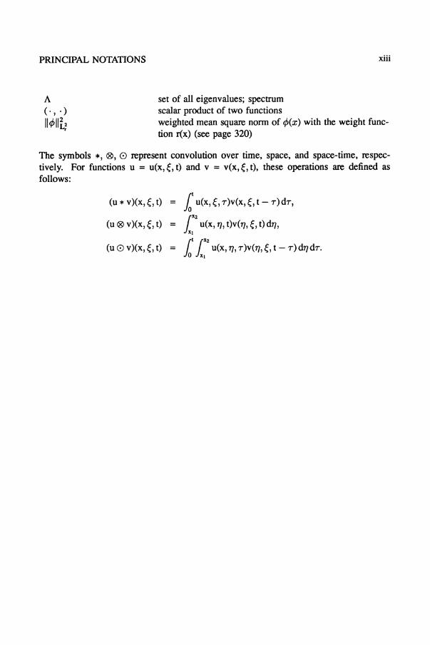
A ( " .)

1Icf>11i:

set of all eigenvalues; spectrum scalar product of two functions weighted mean square norm of cf>(x) with the weight func­tion r(x) (see page 320)

The symbols *, ®, 0 represent convolution over time, space, and space-time, respec­tively. For functions u = u(x,~, t) and v = v(x,~, t), these operations are defined as follows:

(u * v)(x,~, t)

(u ® v)(x,~, t)

(u 0 v)(x,~, t)

= l u(x,~, r)v(x,~, t - r)dr,

= l x2 u(x, 'TI, t)v('TI,~, t) d'TI, Xl

= r l X2 u(x, 'TI, r)v('TI,~, t - r) d'TIdr. Jo Xl

Definitions

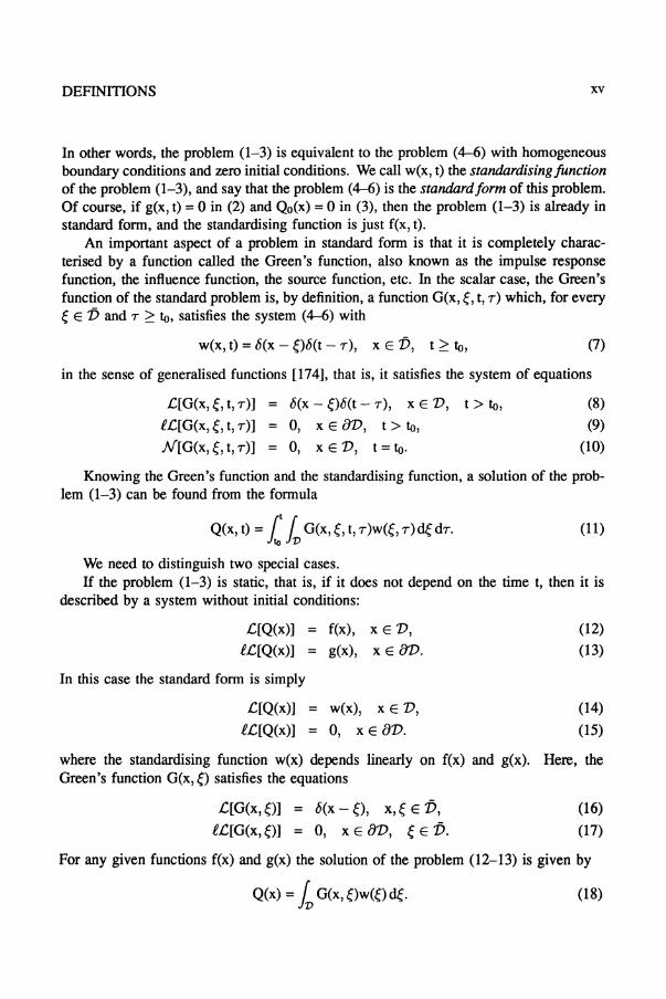
All the boundary and initial value problems listed in this work are expressed in a single standard form, which is defined in this section. Only linear problems are considered.

We are concerned with boundary or initial value problems for differential equations, integral equations and integro-differential equations that describe processes in a specified open set V with a boundary 8V in Euclidean space, and for a time t ~ to where to is some given initial value. We denote by Q(x, t) the unknown function of a problem; in general, it is a vector-function depending on a point x that belongs to an open set V in r-dimensional Euclidean space Er and t ~ to.

To be as general as possible we take the basic equation of a problem in the form

.c[Q(x, t)] = f(x, t), x E V, t > to. (1)

where .c is a linear operator and f(x, t) a given function; the unknown function Q(x, t) is subject to boundary conditions of the form

l[Q(x, t)] = g(x, t), x E av, t > to, (2)

where l is a linear boundary operator and g(x, t) is a given function, and to initial conditions of the form

N[Q(x, t)] = Qo(x), x E V, t = to, (3)

where N is also a linear operator and Qo(x) is a given function. If the basic equation (1) is an integral equation, then conditions (2) and (3) are unnecessary. In the general case the prcblem is to find a vector-function Q(x, t) satisfying (1-3) for given vector-functions f(x, t), g(x, t), and Qo(x).

It can be shown (see [34] and [35, §2.11]) that there is a generalised function or vector- function w(x, t), in general not unique, which depends linearly on f(x, t), g(x, t), and Qo(x), and is such that the problem (1-3) is equivalent to the problem

.c[Q(x, t)] = w(x, t), x E V, t > to, l[Q(x, t)] = 0, x E 8V, t> to,

N[Q(x, t)] = 0, x E V, t = to.

xiv

(4) (5)

(6)

DEFINmONS xv

In other words, the problem (1-3) is equivalent to the problem (4-6) with homogeneous boundary conditions and zero initial conditions. We call w(x, t) the standardising function of the problem (1-3), and say that the problem (4-6) is the standard/orm of this problem. Of course, if g(x, t) = ° in (2) and Qo(x) = ° in (3), then the problem (1-3) is already in standard form, and the standardising function is just f(x, t).

An important aspect of a problem in standard form is that it is completely charac­terised by a function called the Green's function, also known as the impulse response function, the influence function, the source function, etc. In the scalar case, the Green's function of the standard problem is, by definition, a function G(x,~, t, r) which, for every ~ E V and r ~ to, satisfies the system (4-6) with

w(x, t) = t5(x - ~)t5(t - r), x E V, t ~ to, (7)

in the sense of generalised functions [174], that is, it satisfies the system of equations

C[G(x,~, t, r)] = t5(x - ~)t5(t - r), x E V, t > to, t'C[G(x,~, t, r)] = 0, x E av, t> to, N[G(x,~, t, r)] = 0, x E V, t = to.

(8)

(9) (10)

Knowing the Green's function and the standardising function, a solution of the prob­lem (1-3) can be found from the fonnula

Q(x,t)= llvG(x,~,t,r)w(~,r)~dr. (11)

We need to distinguish two special cases. If the problem (1-3) is static, that is, if it does not depend on the time t, then it is

described by a system without initial conditions:

C[Q(x)] = f(x) , x E V,

t'C[Q(x)] = g(x), x E av. In this case the standard form is simply

C[Q(x)] = w(x), x E V,

t'C[Q(x)] = 0, x E 8V.

(12)

(13)

(14)

(15)

where the standardising function w(x) depends linearly on f(x) and g(x). Here, the Green's function G(x,~) satisfies the equations

C[G(x, ~)] = t5(x - ~), x, ~ E V, t'C[G(x,O] = 0, x E 8V, ~ E V.

(16)

(17)

For any given functions f(x) and g(x) the solution of the problem (12-13) is given by

Q(x) = Iv G(x,~)w(~)~. (18)

xvi DEFINITIONS

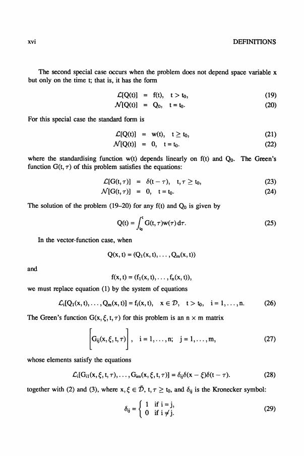
The second special case occurs when the problem does not depend space variable x but only on the time t; that is, it has the fonn

C[Q(t)] = f(t) , t > to, N[Q(t)] = Qo, t = to.

For this special case the standard fonn is

C[Q(t)] = w(t), t ~ to, N[Q(t)] = 0, t = to.

(19)

(20)

(21)

(22)

where the standardising function w(t) depends linearly on f(t) and Qo. The Green's function G(t, T) of this problem satisfies the equations:

C[G(t, T)] = <5(t - T), t, T ~ to, N[G(t, T)] = 0, t = to.

The solution of the problem (19-20) for any f(t) and Qo is given by

Q(t) = l G(t,T)W(T)dT.

In the vector-function case, when

Q(x, t) = (QI (x, t), ... ,Om(x, t»

and f(x, t) = (fl (x, t), ... ,fn(x, t»,

we must replace equation (1) by the system of equations

(23)

(24)

(25)

Ci[QI(X, t), ... , Om(x, t)] = fi(x, t), x E V, t> to, i = 1, ... , n. (26)

The Green's function G(x,~, t, T) for this problem is an n x m matrix

[G,j(X,e,4Tl], i=l, ... ,n; j=l, ... ,m, (27)

whose elements satisfy the equations

(28)

together with (2) and (3), where x, ~ E 1), t, T ~ to, and <5ij is the Kronecker symbol:

{ I if i = j, <5ij = 0 if i i j. (29)

DEFINITIONS

In this case we introduce the idea of a standardising vector-function

w(x, t) = (WI (x, t), ... , wn(x, t»,

and express the solution Q(x, t) in tenns of w(x, t) by a system of the fonn

xvii

Qj(x, t) = [h tGiJ(X,~, t,T)wi(~,T)~dT, j = 1, ... ,m. (30) to v i=l

This is a matrix version of the the solution (11). In the stationary case, that is, when the equations (1-3) are invariant under a trans­

lation along the time axis, the Green's function is represented in the fonn

G(x,~, t, T) = G(x,~, t - T). (31)

Thus it depends only on three variables, and so we can write it as G(x, ~, t). It follows from the 'causality principle' for physical processes that

G(x,~,t,T)=OforxEV, ~E1), t<T. (32)

In particular, for stationary systems,

G(x,~, t) = 0 for x E V, ~ E 1), t < O. (33)

The relations (32) and (33) have a simple physical meaning: the reaction of a physical system to a disturbance cannot occur before the instant the disturbance begins to act.

The transfer function of a stationary problem, denoted W(x,~, p), is obtained by taking the Laplace transfonn with respect to t of G(x,~, t), that is,

W(x,~,p) = G(x,~,p) = 1000 e-plG(x,~, t)dt (34)

where p is a complex variable. It is easily seen that if the problem (1-3), or its equivalent standard form (4-6), is

stationary, then we can take the Laplace transform with respect to t of the equations of the problem straight away. As a result we obtain

£[Q(x, p)] = {(x, p), x E 1),

£[Q(x, p)] = g(x, p), x E av. (35)

(36)

where the complex number p can be regarded as a parameter; here the tilde denotes the Laplace transfonn of the original function with respect to t. The operator £ is obtained by taking the Laplace transfonn of (1) and using the initial conditions (3). The problem (35-36) is a static problem with a parameter p. It can also be reduced to a standard fonn:

£[Q(x, p)] = w(x, p), x E V, £[Q(x, p)] = 0, x E av.

(37)

(38)

xviii DEFINITIONS

where the standardising function w(x, p) depends linearly on f(x, p) and g(x, p). We call the problem (35-36) a spatial boundary value problem. In this case the transfer function W(x,~, p) of (1-3) is the same as the Green's function for the problem (35-36), or the problem (37-38); it is the solution of the system:

£[W(x,~, p)] = 6(x - ~), x, ~ E D, f[W(x,~, p)] = 0, x E av, ~ E D.

(39)

(40)

We can associate with each boundary value problem (39-40) a certain system (denu­merable or nondenumerable) of eigenfunctions ch.(x) and eigenvalues Ab defined as the solution of the system

£ [</>k (x)]

f[</>k(X)]

(41)

(42)

In the main text, as well as standardising functions, Green's functions and transfer functions, we mention several other functions and numbers: the eigenfunctions of a given boundary value problem and of its adjoint problem, eigenvalues, spatial eigenfrequencies (wave numbers), temporal eigenfrequencies, and the relations between these (dispersion relations), and normalising weight functions for the eigenfunctions of a given problem. The physical significance of these concepts is well documented in textbooks and mono­graphs, examples of which are given in the bibliography. An overview of these topics from the point of view of finite integral transforms is presented in chapter 3 of this book.

The system of classification of problems

The system of classification of problems used in this book follows the same classification scheme as the previous work [35]. This system applies both to problems involving individual differential equations and to systems of differential equations. The problems are divided into groups, each group being labelled with a triple of integers (r.m.n), where

r is the dimension of the spatial domain of definition V of the function Q in a given problem;

m is the order of the highest derivative of Q with respect to t in the basic equation;

n is the order of the highest derivative of Q with respect to spatial variables in the basic equation.

This book presents detailed characteristics for individual equations of thirteen groups in chapter 1, and for systems of equations of four groups in chapter 2. Differential­difference equations, integral equations, integro-differential equations, and systems of integral equations are grouped in separate sections.

xix