- 1 -

Characteristics of File System Workloads

Drew Roselli and Thomas E. Anderson

Abstract

In this report, we describe the collection of file system traces from three different environ-

ments. By using the auditing system to collect traces on client machines, we are able to get

detailed traces with minimal kernel changes. We then present results of traffic analysis on the

traces, contrasting them with those from previous studies. Based on these results, we argue

that file systems must optimize disk layout for good read performance.

1 Introduction

Many new file system designs are currently being proposed as a result of changes in the

relative performance of the underlying hardware. Because processor performance is increas-

ing much more rapidly than disk performance, file systems are commensurately being pres-

sured to employ techniques to avoid or decrease the impact of disk accesses. While the file

systems of the 80’s, such as FFS[12], used simple disk configurations and layout policies,

today’s file systems are exploring more complicated techniques in order to eke all possible

performance out of available resources. For example, cooperative caching uses remote mem-

ory rather than local disk whenever possible [4][6], disk striping is used to achieve higher

bandwidth than is possible with a single disk [2][9], and write-ahead logging is used to avoid

seeks [20]. Increased processor performance relative to disk performance also tips the bal-

ance in favor of spending more cycles to evaluate more complicated algorithms.

During the course of our research in file system design, we were hindered by the dearth of

information on long-term file system behavior. The two primary methods for evaluating file

system design are benchmarks and traces. Benchmarks are useful for evaluating specific

workloads but may not reflect realistic workloads. More importantly, because the input is ar-

tificial, they cannot be used to understand long-term behavior. On the other hand, evaluation

by replaying traces has its own set of difficulties. Traces are necessarily bound to the envi-

ronment from which they were collected, and because computing environments change rap-

- 2 -

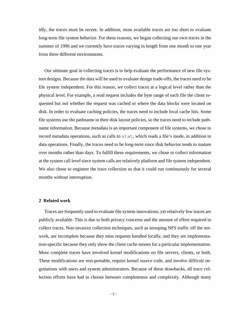
idly, the traces must be recent. In addition, most available traces are too short to evaluate

long-term file system behavior. For these reasons, we began collecting our own traces in the

summer of 1996 and we currently have traces varying in length from one month to one year

from three different environments.

Our ultimate goal in collecting traces is to help evaluate the performance of new file sys-

tem designs. Because the data will be used to evaluate design trade-offs, the traces need to be

file system independent. For this reason, we collect traces at a logical level rather than the

physical level. For example, a read request includes the byte range of each file the client re-

quested but not whether the request was cached or where the data blocks were located on

disk. In order to evaluate caching policies, the traces need to include local cache hits. Some

file systems use the pathname in their disk layout policies, so the traces need to include path-

name information. Because metadata is an important component of file systems, we chose to

record metadata operations, such as calls tostat , which reads a file’s inode, in addition to

data operations. Finally, the traces need to be long-term since disk behavior tends to mature

over months rather than days. To fulfill these requirements, we chose to collect information

at the system call level since system calls are relatively platform and file system independent.

We also chose to engineer the trace collection so that it could run continuously for several

months without interruption.

2 Related work

Traces are frequently used to evaluate file system innovations, yet relatively few traces are

publicly available. This is due to both privacy concerns and the amount of effort required to

collect traces. Non-invasive collection techniques, such as snooping NFS traffic off the net-

work, are incomplete because they miss requests handled locally, and they are implementa-

tion-specific because they only show the client cache misses for a particular implementation.

More complete traces have involved kernel modifications on file servers, clients, or both.

These modifications are non-portable, require kernel source code, and involve difficult ne-

gotiations with users and system administrators. Because of these drawbacks, all trace col-

lection efforts have had to choose between completeness and complexity. Although many

- 3 -

researchers have published work based on private traces, in this section, we restrict our dis-

cussion to publicly available traces.

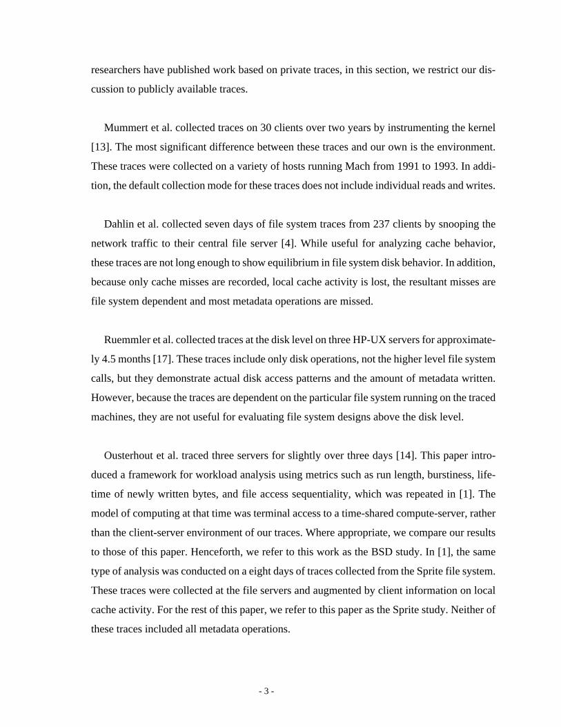
Mummert et al. collected traces on 30 clients over two years by instrumenting the kernel

[13]. The most significant difference between these traces and our own is the environment.

These traces were collected on a variety of hosts running Mach from 1991 to 1993. In addi-

tion, the default collection mode for these traces does not include individual reads and writes.

Dahlin et al. collected seven days of file system traces from 237 clients by snooping the

network traffic to their central file server [4]. While useful for analyzing cache behavior,

these traces are not long enough to show equilibrium in file system disk behavior. In addition,

because only cache misses are recorded, local cache activity is lost, the resultant misses are

file system dependent and most metadata operations are missed.

Ruemmler et al. collected traces at the disk level on three HP-UX servers for approximate-

ly 4.5 months [17]. These traces include only disk operations, not the higher level file system

calls, but they demonstrate actual disk access patterns and the amount of metadata written.

However, because the traces are dependent on the particular file system running on the traced

machines, they are not useful for evaluating file system designs above the disk level.

Ousterhout et al. traced three servers for slightly over three days [14]. This paper intro-

duced a framework for workload analysis using metrics such as run length, burstiness, life-

time of newly written bytes, and file access sequentiality, which was repeated in [1]. The

model of computing at that time was terminal access to a time-shared compute-server, rather

than the client-server environment of our traces. Where appropriate, we compare our results

to those of this paper. Henceforth, we refer to this work as the BSD study. In [1], the same

type of analysis was conducted on a eight days of traces collected from the Sprite file system.

These traces were collected at the file servers and augmented by client information on local

cache activity. For the rest of this paper, we refer to this paper as the Sprite study. Neither of

these traces included all metadata operations.

- 4 -

A combination of features distinguish our traces from the above work. First, our traces are

long term. Because file system factors such as disk fragmentation mature over time [12][19],

long term traces are necessary to evaluate disk layout policies. Second, our traces include

three different workloads and include detailed traces of a database web server. Third, indi-

vidual reads and writes are recorded so that detailed information on access patterns is avail-

able. Fourth, since metadata operations have a significant impact on disk requests [17], our

traces include metadata operations. In addition, our traces include full pathnames for file ref-

erences andexec system calls are traced so that it is possible to investigate applications that

cause file system activity. Finally, because our traces were recently collected, we can com-

pare our results with those of previous studies to illustrate patterns in file system activity over

time.

3 Trace Collection

3.1 Environment

We traced three groups of Hewlett-Packard series 700 workstations running HP-UX 9.05.

The first group consisted of twenty machines located in laboratories for undergraduate class-

es. For the rest of this paper, we refer to this workload as the Instructional Workload (INS).

The second group consists of 13 machines on the desktops of graduate students, faculty, and

administrative staff of our research group project. We refer to this workload as the Research

Workload (RES). Because the users of the RES cluster have a large (untraced) collection of

workstations at their disposal, their (traced) desktop machines are relatively idle. The third

set of traces was collected from a single machine that is the web server for an online library

project.This host maintains a database of images using the Postgres database management

system and exports the images via its web interface. This server receives approximately 2300

accesses per day. We refer to this workload as the WEB workload. The INS machines mount

home directories and common binaries from a non-traced Hewlett-Packard workstation. All

other machines mount home directories and common binaries from an Auspex server over an

Ethernet. We collected eight months of traces from the INS cluster (two semesters), one year

of traces from the RES cluster, and approximately one month of traces from the WEB host.

- 5 -

Each host has 64MB of memory. The file cache size on these hosts at the time of trace

collection is unknown. However, since HP-UX 10 allows a maximum of half of memory to

be used by the file cache, we can assume that the file cache was maximally 32MB.

3.2 Methodology: The Auditing System

To minimize kernel changes, we used the auditing subsystem to record file system events.

Many operating systems include an auditing subsystem for security purposes. The auditing

subsystem gets invoked after a system call and is configured to log specified system calls

with their arguments and return values. This is ideal for tracing since it catches the logical

level of requests using already existing kernel functionality, however it does not record ker-

nel file system activity, such as paging executables. The major problem we faced in using the

auditing system was that the HP-UX version records pathnames exactly as specified by the

user. Users often specify paths relative to their current working directory rather than the com-

plete path. Since some file system policies, such as disk layout, use a file’s parent directory,

we needed to record the full pathname. We solved this problem by recording the current

working directory’s pathname for each process and configuring the auditing system to catch

all system calls capable of changing the current working directory. These changes required

only small changes to the kernel (about 350 of lines of C code) and were wholly contained

within the auditing subsystem.

3.3 Impact on Client Resources

On the host being traced, the log files are changed and compressed every hour by acron

script. The compressed traces use on average 3.2MB of local disk space per day. The trace

files are migrated off the client nightly over an Ethernet to a collection host. Hosts send off

their trace files at staggered one minute intervals so that the network and receiving host are

not overwhelmed. Assuming an Ethernet’s effective bandwidth to be 5Mbps, sending 3.2MB

per minute uses less than 10% of the network capacity.

In order for trace collection to be tolerated by the users, it must have minimal impact on

- 6 -

the performance and resource usage of the machine being traced. We measured the overhead

of our tracing system on a compilation workload. Originally, the tracing code added 11%

overhead compared with the same benchmark without tracing. However, by buffering trace

records in the kernel and writing them out in large batches, we were able to reduce the over-

head to 1%.

3.4 Trace Format

The format of the trace records is shown in Figure 1. Each record contains a header fol-

lowed by arguments. The header is a fixed length and contains six fields. The first field con-

tains the time the record was generated measured in seconds since January 1, 1970. The

following fields identify the host, user, and process that generated the record. The next field

contains the system call type. The system call type determines the number and type of any

arguments following the header. The last header field contains the length in bytes of all the

arguments for the record. In the raw traces, the arguments are those that are provided by the

system call. During postprocessing (described in the next section), some of the arguments are

changed. For example, file descriptor arguments are replaced by identifiers for the files they

reference. The complete list of traced calls and their arguments is enumerated in the Appen-

dix.

FIGURE 1. Trace Record Format.All trace records contain a header followed by any arguments. Thenumber and type of arguments is determined by the system call type. A complete list of system callstraced and their arguments is shown in the Appendix. For the raw traces, the arguments are the same asthose specified by the system call.

time

host id

user id

process id

system call number

length of all arguments

argument 1

...

argumentn

- 7 -

3.5 Postprocessing

For easier use in replaying traces, the trace files are postprocessed to assign unique iden-

tifiers to files, match file descriptors to file identifiers, and fix a number of problems in the

raw traces.

During postprocessing, each pathname is assigned a device number by consulting a static

table of mount paths. This is the least automated and therefore most fragile part of postpro-

cessing; it requires checking the mount tables of each client by hand and incorporating the

mounted systems into the postprocessing code. Files accessed through symbolic links that

span file systems are incorrectly recorded as if the data were stored on the file system of the

symbolic link rather than the file system where the data actually reside. We measured the

number of such symbolic links on several of our file systems and found them to be less than

1% of all files, so we do not believe this inaccuracy significantly affects results generated

from the traces.

Once the device has been determined, a file identifier is assigned. A givendevice-fileid

pair is unique throughout the trace. File descriptors are then mapped onto these device-fileid

pairs. If the postprocessor cannot match a file descriptor to a fileid, the fileid is set toUN-

KNOWN. Many unknown files are caused byfstat calls to files opened by system processes

that start before the auditing system when the host is booted; because anfstat call only

contains a file descriptor, if the file’s open is missed, subsequent calls cannot be matched to

the file to which the descriptor refers. The number of records referring to unknown files is

3% for INS, 10% for RES, and 0.1% for WEB. For RES, 97% of records containing unknown

files arefstat calls. For all workloads, the number of reads and writes to unknown files is

less than 1%.

Another task of postprocessing is to fix problems with the raw traces. One of the most in-

sidious problems is handling corrupted records. Corrupted records are caused when the log-

ging of an audit record is interrupted by another system call or when the auditing system is

- 8 -

switched on or off. To eliminate these records, the postprocessor checks the range of values

of several header and argument fields. Any record containing a field with an invalid value is

removed. We detect that less than 0.01% of the trace records are corrupted. While this rate is

acceptably low, a single error can cause the rest of the trace file to become unreadable. To

prevent this cascading effect, the postprocessor checks several fields of the record header. If

a header fails the check, the trace file is scanned for the next legitimate header and postpro-

cessing then continues.

In order to preserve privacy, the user identifier is altered by a one-way mapping function

as the traces are processed. However, user identifiers zero through ten are not altered since

these accounts are administrative in nature rather than personal and may provide insight to

the trace analysis. Because pathnames themselves may compromise privacy, once a file is

given a unique identifier, its pathname is removed from the traces and stored in a separate

file.

Finally, the postprocessor removes most of the trace records caused by the trace collection

process—for example, file writes to the log file. Postprocessing reduces these extra records

to only 0.04% of the postprocessed traces on an average machine. We do not remove all of

the residual trace records because this would significantly complicate the postprocessing

code. None of the remaining calls are reads or writes.

3.6 Scalability

A goal in designing the trace collection infrastructure was that it be scalable to at least 150

hosts, so that the number of hosts we could trace would not be dependent on our ability to

store and process the traces. In terms of storage, the compressed, unprocessed traces require

on average 3.2MB per host per day. Therefore, tracing 150 hosts for 6 months would require

less than 100GB of disk space.

The second component of scalability is in the processing phase. Processing is divided into

two major phases: a parallel phase and a sequential phase. The parallel phase is performed

- 9 -

on the individual client traces before they are merged together. To maximize parallelism, as

much work as possible is done in this phase. The traces are then merged together by times-

tamp and the sequential phase begins. The only operations that must be done sequentially are

the assignment of fileids to nonlocal file systems and the mapping of file descriptors to these

fileids. Obviously, it is the sequential phase that limits the scalability of postprocessing. The

sequential phase processes one day of traces for 30 hosts in about 30 minutes. This phase

scales linearly with the number of hosts, so it could process one day of traces from 150 hosts

in about 2.5 hours.

3.7 Limitations of Methodology

The benefits of using the auditing system as a tracing tool are that it provides a method of

collecting a complete set of file system calls with low overhead and only small changes to

the kernel. In fact, with nominal vendor support, any type of system call could be traced with-

out modifying the kernel at all. Another solution would be to use a mechanism to intercept

system calls, such as SLIC [7], to record system calls.

Advantages of collecting the traces on the clients rather on the server are that local cache

hits are included and no burden is added to the server which is often the bottleneck in distrib-

uted file systems. But recording on the client requires the tracing code to be installed on many

machines and complicates processing since all the individual traces must be merged. In our

environment, no machines that acted as file servers were traced. However, unless all clients

are traced, it is possible to miss accesses to files from non-traced hosts. Although we did not

collect traces on all clients, for the clusters traced, most users tend to use the same host (or

set of hosts) regularly, so it is likely that most activity for a given user of the cluster is col-

lected.

Since the traces are taken at the system call level, file system requests internal to the kernel

are not recorded. As a result, pathname lookup, reads and writes to memory mapped regions,

and file closes that occur during anexec system call are not included. Measurements by [17]

show disk paging to swap partitions to be 0.4–16.5% of all disk traffic, however the impact

of the kernel reading executable and memory-mapped files is unknown.

- 10 -

Finally, although our original intention in recording complete pathnames was to record the

parent directory, having this information has proven invaluable to understanding the traces

and the applications that cause specific file traffic patterns.

4 Results

Unless otherwise specified, the results presented in this report are based on 112 days of

traces (September 11, 1996 to December 31, 1996) for the INS and RES workloads. The in-

structional cluster is affected by Berkeley’s course schedule; activity on this cluster drops

during the second half of December and many system administration tasks are accomplished

during this time. The WEB trace results consist of 25 days (January 23, 1997 to February 16,

1997). Since other activity occurs on the WEB host than the workload we are interested in,

the WEB traces are filtered to include only the userid of the web service and database service

daemons, as well as administrative userids, such as root. Due to the volume of the data col-

lected, some results are based on sampled days from the described intervals. For INS and

RES, we sampled eight days spaced 13 days apart so that all days of the week are represented.

Because the WEB traces are shorter, we sample five days spaced six days apart. All results

based on only sampled days are explicitly noted.

Since file cache misses are far more expensive than cache hits, understanding miss traffic

is vital to understanding file system performance. For this purpose, we developed a simple

cache simulator that contains a read cache and write buffer. The read cache takes as param-

eters a blocksize and a memory size and maintains a local, LRU-based cache for each host.

The write buffer is also local to each host and, unless otherwise specified, holds up to 4MB

of writes that are less than 30 seconds old.Sync andfsync calls in the traces flush the ap-

propriate files from the write buffer. The simulator output consists of blocks of reads that did

not hit in the cache or write buffer and writes that are older than 30 seconds. Unless otherwise

specified, the simulator is not configured to do prefetching.

For some of our results, reads to an irregularly accessed file, namedaudio.sec , are

- 11 -

omitted. This file is used by the programasecure, which controls access to the machine’s

audio system. It reads and writes small records toaudio.sec using thefread library call

(which chunks reads and writes into 8kB requests) and then seeks to the next record. As a

result,audio.sec is typically read in overlapping chunks of 8kB chunks. An example of

the read pattern of this file is a request to read bytes 0 through 8192, followed by a request to

read bytes 3 through 8195, etc. In this manner, the file appears to produce enormous band-

width—in many cases, overshadowing all other activity—yet the application has not read

many distinct bytes. We excise all accesses to this file from results generated from the raw

traces. Since most of these accesses are absorbed by the cache, results based on cache-filtered

data do not excise this file.

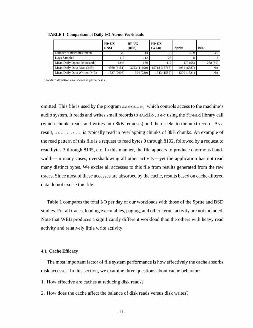
Table 1 compares the total I/O per day of our workloads with those of the Sprite and BSD

studies. For all traces, loading executables, paging, and other kernel activity are not included.

Note that WEB produces a significantly different workload than the others with heavy read

activity and relatively little write activity.

4.1 Cache Efficacy

The most important factor of file system performance is how effectively the cache absorbs

disk accesses. In this section, we examine three questions about cache behavior:

1. How effective are caches at reducing disk reads?

2. How does the cache affect the balance of disk reads versus disk writes?

TABLE 1. Comparison of Daily I/O Across Workloads

Standard deviations are shown in parentheses.

HP-UX(INS)

HP-UX(RES)

HP-UX(WEB) Sprite BSD

Number of machines traced 20 14 1.0 39.9 3.0

Days Sampled 112 112 25 8 3

Mean Daily Opens (thousands) 1246 139 412 170 (55) 268 (59)

Mean Daily Data Read (MB) 4360 (5181) 3753 (11190) 15718 (16768) 4954 (6587) NA

Mean Daily Data Written (MB) 1337 (2003) 394 (230) 1743 (1582) 1200 (1521) NA

- 12 -

3. How effective are caches at reducing disk seeks?

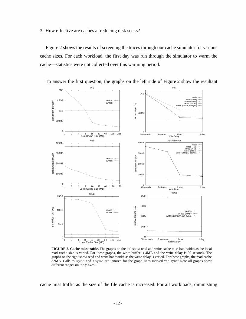
Figure 2 shows the results of screening the traces through our cache simulator for various

cache sizes. For each workload, the first day was run through the simulator to warm the

cache—statistics were not collected over this warming period.

To answer the first question, the graphs on the left side of Figure 2 show the resultant

cache miss traffic as the size of the file cache is increased. For all workloads, diminishing

0

500MB

1GB

1.5GB

2GB

1 2 4 8 16 32 64 128 256

Ban

dwid

th p

er D

ay

Local Cache Size (MB)

INS

readswrites

FIGURE 2. Cache miss traffic.The graphs on the left show read and write cache miss bandwidth as the localread cache size is varied. For these graphs, the write buffer is 4MB and the write delay is 30 seconds. Thegraphs on the right show read and write bandwidth as the write delay is varied. For these graphs, the read cache32MB. Calls tosync and fsync are ignored for the graph lines marked “no sync”.Note all graphs showdifferent ranges on the y-axes.

0

100MB

200MB

300MB

400MB

1 2 4 8 16 32 64 128 256

Ban

dwid

th p

er D

ay

Local Cache Size (MB)

RES

readswrites

0

5GB

10GB

15GB

1 2 4 8 16 32 64 128 256

Ban

dwid

th p

er D

ay

Local Cache Size (MB)

WEB

readswrites

0

100MB

200MB

300MB

400MB

30 seconds 5 minutes 1 hour 1 day

Ban

dwid

th p

er D

ay

Write Delay

RES Workload

readswrites (4MB)

writes (16MB)writes (infinite)

writes (infinite, no sync)

0

2GB

4GB

6GB

8GB

30 seconds 5 minutes 1 hour 1 day

Ban

dwid

th p

er D

ay

Write Delay

WEB

readswrites (4MB)

writes (infinite, no sync)

0

500MB

1GB

30 seconds 5 minutes 1 hour 1 dayB

andw

idth

per

Day

Write Delay

INS

readswrites (4MB)

writes (16MB)writes (infinite)

writes (infinite, no sync)

- 13 -

returns can be seen at large cache sizes.

It has been argued that disk layout should be optimized for writes since they dominate disk

traffic when there is a large file cache [16]. Indeed, Figure 2 shows that the balance of read

and write disk traffic changes significantly with larger caches. Since the WEB workload has

few writes, its disk traffic is dominated by reads even with large caches. However, the INS

and RES workloads have more than double the write traffic relative to read traffic at the

256MB cache size. Since many newly created bytes have a short lifetime (see Section 4.2),

file systems may avoid disk accesses by increasing the write delay for asynchronous writes

or using NVRAM (which effectively increases the write delay without loss of reliability) or

reliable memory [3]. The graphs on the right side of Figure 2 show the effect of increasing

the write delay with write buffer sizes of 4MB and 16MB and for an infinitely sized write

buffer. For all workloads, the 16MB write buffer performs close to the infinitely sized write

buffer. For both RES and INS, with a 16MB write buffer and 32MB read cache, disk read

and write bandwidth is about the same. Since the latency of write traffic can often be hidden

from the application by writing data asynchronously or by using a write-ahead log or log-

structured file system, the performance of disk reads is likely to have more impact on appli-

cation performance.

Since disk bandwidth is improving faster than disk latency, a critical metric in evaluating

cache performance is the number of seeks caused by cache misses. A rough estimate for

counting the number of seeks isfileios, the number of different file block accesses. Within a

stream of cache misses, if a cache miss is in the same file as the previous cache miss, no fileio

is counted; otherwise, the number of fileios is incremented by one. This is a crude metric, but

assuming files are stored sequentially on disk and that the disk track buffer can quickly return

blocks from the same file, we believe it is a more accurate measure of disk latency than sim-

ply countingblockios, which counts every block that misses the cache (calleddiskios in [14]).

Similarly, we count adirio every time a cache miss is accessed that is in a different directory

than that of the previous cache miss. This is similar tocylinder groups in FFS, in which

neighboring disk cylinders are collected into groups and files in the same directory are placed

- 14 -

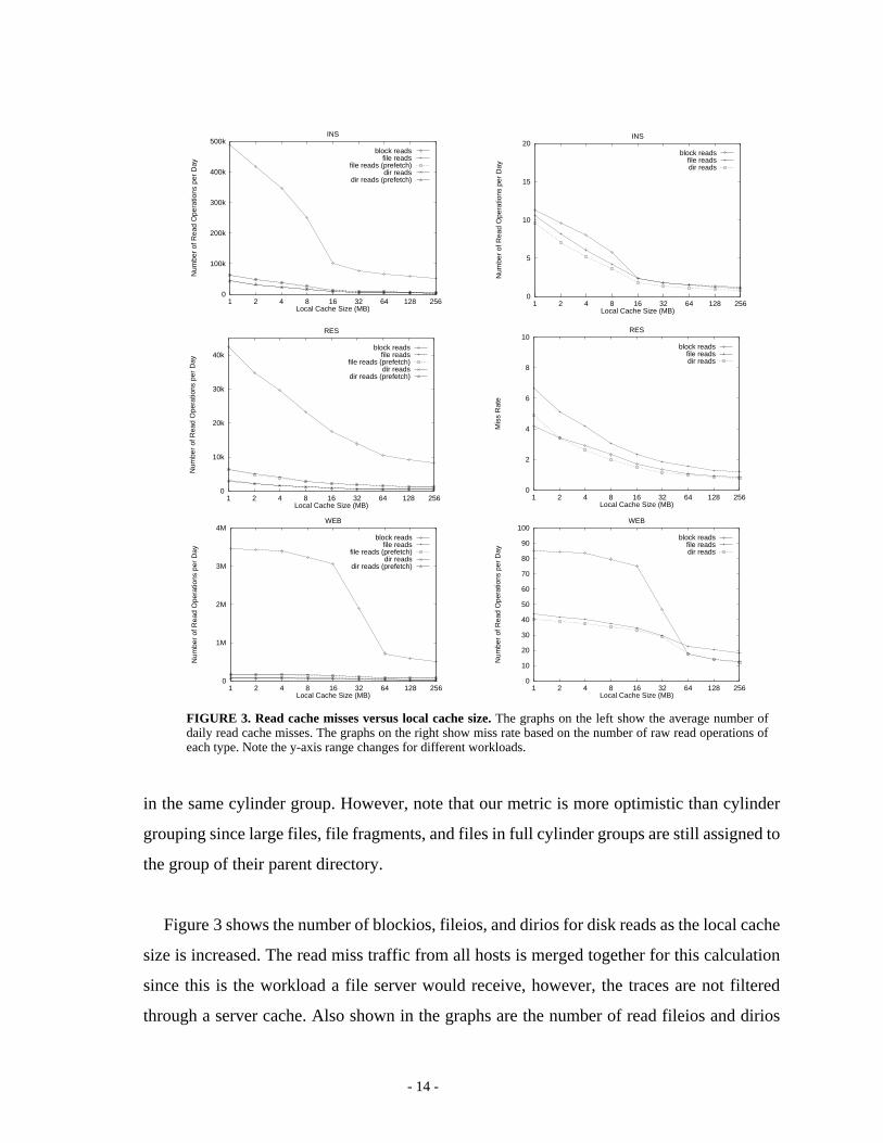
in the same cylinder group. However, note that our metric is more optimistic than cylinder

grouping since large files, file fragments, and files in full cylinder groups are still assigned to

the group of their parent directory.

Figure 3 shows the number of blockios, fileios, and dirios for disk reads as the local cache

size is increased. The read miss traffic from all hosts is merged together for this calculation

since this is the workload a file server would receive, however, the traces are not filtered

through a server cache. Also shown in the graphs are the number of read fileios and dirios

0

5

10

15

20

1 2 4 8 16 32 64 128 256

Num

ber

of R

ead

Ope

ratio

ns p

er D

ay

Local Cache Size (MB)

INS

block readsfile readsdir reads

0

2

4

6

8

10

1 2 4 8 16 32 64 128 256M

iss

Rat

eLocal Cache Size (MB)

RES

block readsfile readsdir reads

0

10

20

30

40

50

60

70

80

90

100

1 2 4 8 16 32 64 128 256

Num

ber

of R

ead

Ope

ratio

ns p

er D

ay

Local Cache Size (MB)

WEB

block readsfile readsdir reads

0

100k

200k

300k

400k

500k

1 2 4 8 16 32 64 128 256

Num

ber

of R

ead

Ope

ratio

ns p

er D

ay

Local Cache Size (MB)

INS

block readsfile reads

file reads (prefetch)dir reads

dir reads (prefetch)

0

10k

20k

30k

40k

1 2 4 8 16 32 64 128 256

Num

ber

of R

ead

Ope

ratio

ns p

er D

ay

Local Cache Size (MB)

RES

block readsfile reads

file reads (prefetch)dir reads

dir reads (prefetch)

0

1M

2M

3M

4M

1 2 4 8 16 32 64 128 256

Num

ber

of R

ead

Ope

ratio

ns p

er D

ay

Local Cache Size (MB)

WEB

block readsfile reads

file reads (prefetch)dir reads

dir reads (prefetch)

FIGURE 3. Read cache misses versus local cache size.The graphs on the left show the average number ofdaily read cache misses. The graphs on the right show miss rate based on the number of raw read operations ofeach type. Note the y-axis range changes for different workloads.

- 15 -

when the cache simulator is configured with prefetching. The prefetching policy used for

these results fetches eight blocks at a time when a file is first opened or is being accessed se-

quentially. Note that prefetching does not noticeably change the number of read fileios or di-

rios for any workload. This indicates that read requests for separate files are rarely

interleaved even with small caches.

The graphs on the right side of Figure 3 show the miss rate for each, where the miss rate

is calculated as the percent of raw operations that are not eliminated by the cache. For all

workloads, increasing cache size has a larger effect on decreasing blockios than fileios or di-

rios. This suggests that larger caches have less benefit than might appear from the block

cache hit rate.

In this section, we have shown that by using persistent memory to increase write delay,

disk write traffic can be significantly stemmed. However, for reads the results are less prom-

ising. There are diminishing returns on increasing cache size to reduce disk reads. Further,

when seeks are estimated using fileios, the point of diminishing returns begins sooner than

when read bandwidth is used.

4.2 File Lifetime

In this section, we examine file lifetime, which we define to be the time between a file’s

creation and its deletion. Knowing the average file lifetime for a workload can aid in deter-

mining appropriate write delay times and deciding how long to wait before reorganizing data

on disk. Our initial results indicated that most dead blocks are overwritten rather than deleted

or truncated. To include the effects of overwrites, we measured byte lifetime rather than file

lifetime in Figure 5.

We calculate lifetime by subtracting the byte’s creation time from its deletion time. This

is different from the “deletion-based” method used by [1] in which all deleted files are

tracked and lifetime is calculated by subtracting the file’s deletion time from its creation time.

In our “creation-based” method, a trace is divided into two halves. All files created within the

- 16 -

first half of the trace are tracked. If a tracked file is deleted during either the first or second

half of the trace, its lifetime is calculated by subtracting the deletion time from the creation

time. If a tracked file is not deleted during the trace, the file is known to have lived for at least

half the duration of the trace. The main difference between the creation-based and deletion-

based methods is the files that are used to generate the results. Because the deletion-based

method bases its data on files that are deleted, it provides more accurate information on the

lifetime distribution of files that are deleted. However, it is not appropriate to generalize from

this data the lifetime distribution of newly created files. Because we are interested in knowing

the lifetime distribution of newly created files, we use the creation-based algorithm for all

results in this section so that the data can be used to predict lifetimes of newly created files.

One drawback of this approach is that it only provides accurate lifetime data for lifetimes less

than half the duration of the trace, however, since our traces are on the order of months, we

are able to acquire lifetime data sufficient for our purposes. Figure 4 shows the difference in

results of create-based and delete-based methods on the Sprite traces. Due to the difference

in sampled files, the delete-based method calculates a shorter lifetime than the create-based

method.

- 17 -

Figure 5 shows the results of using the create-based method on our workloads. Except for

10

20

30

40

50

60

70

80

90

100

30 seconds5 minutes 1 hour 1 day

Cum

ulat

ive

Per

cent

age

of B

ytes

Lifetime (Seconds)

Trace 1-2

delete-basedcreate-based

FIGURE 4. Create-based versus delete-based lifetime calculations for the Sprite traces.These graphsshow byte lifetime for lifetime values calculated using a create-based algorithm and a delete-based algorithm.Unlike the results reported in [1], all results include blocks overwritten to files that were not deleted andlifetime is calculated based on exact byte-ranges rather than blocks, however, these differences have onlyminor effects on the results.

10

20

30

40

50

60

70

80

90

100

30 seconds5 minutes 1 hour 1 day

Cum

ulat

ive

Per

cent

age

of B

ytes

Lifetime (Seconds)

Trace 3-4

delete-basedcreate-based

10

20

30

40

50

60

70

80

90

100

30 seconds5 minutes 1 hour 1 day

Cum

ulat

ive

Per

cent

age

of B

ytes

Lifetime (Seconds)

Trace 5-6

delete-basedcreate-based

10

20

30

40

50

60

70

80

90

100

30 seconds5 minutes 1 hour 1 day

Cum

ulat

ive

Per

cent

age

of B

ytes

Lifetime (Seconds)

Trace 7-8

delete-basedcreate-based

0

10

20

30

40

50

60

70

80

90

100

1 sec 30 sec 5 min 1 hour 1 day 30 days

Cum

ulat

ive

Per

cent

age

of B

ytes

Byte Lifetime

InsRes

WebSprite

FIGURE 5. Byte lifetime. This graph shows theresults of using the create-based lifetime calculationmethod.

- 18 -

the INS workload, most newly-created bytes live significantly longer than 30 seconds. This

implies that a longer write delay must be used to effectively stem disk write traffic.

In addition to calculating lifetimes over our traces, we wanted to get a more in depth pic-

ture of which files get deleted. Specifically, we wanted to know:

1. Are delete patterns constant over the long-term?

2. Can we predict which files are likely to be deleted?

3. Is file lifetime related to file size?

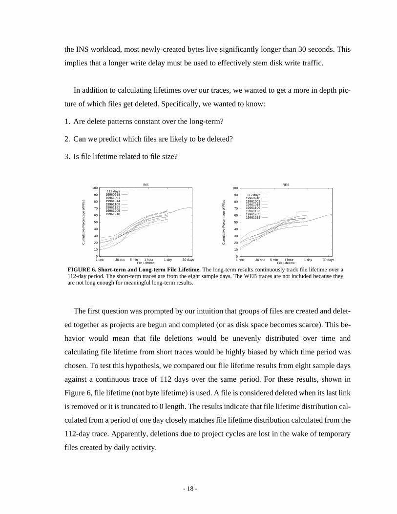
The first question was prompted by our intuition that groups of files are created and delet-

ed together as projects are begun and completed (or as disk space becomes scarce). This be-

havior would mean that file deletions would be unevenly distributed over time and

calculating file lifetime from short traces would be highly biased by which time period was

chosen. To test this hypothesis, we compared our file lifetime results from eight sample days

against a continuous trace of 112 days over the same period. For these results, shown in

Figure 6, file lifetime (not byte lifetime) is used. A file is considered deleted when its last link

is removed or it is truncated to 0 length. The results indicate that file lifetime distribution cal-

culated from a period of one day closely matches file lifetime distribution calculated from the

112-day trace. Apparently, deletions due to project cycles are lost in the wake of temporary

files created by daily activity.

0

10

20

30

40

50

60

70

80

90

100

1 sec 30 sec 5 min 1 hour 1 day 30 days

Cum

ulat

ive

Per

cent

age

of F

iles

File Lifetime

INS

112 days19960918199610011996101419961109199611221996120519961218

FIGURE 6. Short-term and Long-term File Lifetime. The long-term results continuously track file lifetime over a112-day period. The short-term traces are from the eight sample days. The WEB traces are not included because theyare not long enough for meaningful long-term results.

0

10

20

30

40

50

60

70

80

90

100

1 sec 30 sec 5 min 1 hour 1 day 30 days

Cum

ulat

ive

Per

cent

age

of F

iles

File Lifetime

RES

112 days19960918199610011996101419961109199611221996120519961218

- 19 -

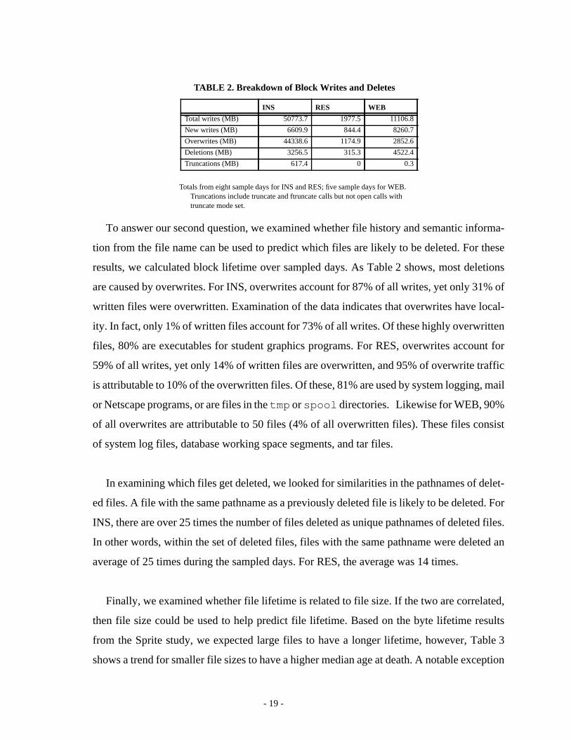
To answer our second question, we examined whether file history and semantic informa-

tion from the file name can be used to predict which files are likely to be deleted. For these

results, we calculated block lifetime over sampled days. As Table 2 shows, most deletions

are caused by overwrites. For INS, overwrites account for 87% of all writes, yet only 31% of

written files were overwritten. Examination of the data indicates that overwrites have local-

ity. In fact, only 1% of written files account for 73% of all writes. Of these highly overwritten

files, 80% are executables for student graphics programs. For RES, overwrites account for

59% of all writes, yet only 14% of written files are overwritten, and 95% of overwrite traffic

is attributable to 10% of the overwritten files. Of these, 81% are used by system logging, mail

or Netscape programs, or are files in thetmp orspool directories. Likewise for WEB, 90%

of all overwrites are attributable to 50 files (4% of all overwritten files). These files consist

of system log files, database working space segments, and tar files.

In examining which files get deleted, we looked for similarities in the pathnames of delet-

ed files. A file with the same pathname as a previously deleted file is likely to be deleted. For

INS, there are over 25 times the number of files deleted as unique pathnames of deleted files.

In other words, within the set of deleted files, files with the same pathname were deleted an

average of 25 times during the sampled days. For RES, the average was 14 times.

Finally, we examined whether file lifetime is related to file size. If the two are correlated,

then file size could be used to help predict file lifetime. Based on the byte lifetime results

from the Sprite study, we expected large files to have a longer lifetime, however, Table 3

shows a trend for smaller file sizes to have a higher median age at death. A notable exception

Totals from eight sample days for INS and RES; five sample days for WEB.Truncations include truncate and ftruncate calls but not open calls withtruncate mode set.

TABLE 2. Breakdown of Block Writes and Deletes

INS RES WEB

Total writes (MB) 50773.7 1977.5 11106.8

New writes (MB) 6609.9 844.4 8260.7

Overwrites (MB) 44338.6 1174.9 2852.6

Deletions (MB) 3256.5 315.3 4522.4

Truncations (MB) 617.4 0 0.3

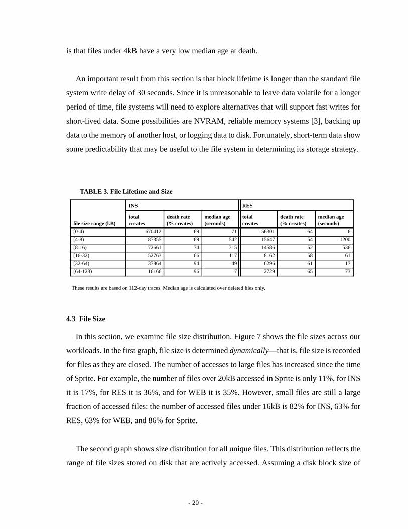
- 20 -

is that files under 4kB have a very low median age at death.

An important result from this section is that block lifetime is longer than the standard file

system write delay of 30 seconds. Since it is unreasonable to leave data volatile for a longer

period of time, file systems will need to explore alternatives that will support fast writes for

short-lived data. Some possibilities are NVRAM, reliable memory systems [3], backing up

data to the memory of another host, or logging data to disk. Fortunately, short-term data show

some predictability that may be useful to the file system in determining its storage strategy.

4.3 File Size

In this section, we examine file size distribution. Figure 7 shows the file sizes across our

workloads. In the first graph, file size is determineddynamically—that is, file size is recorded

for files as they are closed. The number of accesses to large files has increased since the time

of Sprite. For example, the number of files over 20kB accessed in Sprite is only 11%, for INS

it is 17%, for RES it is 36%, and for WEB it is 35%. However, small files are still a large

fraction of accessed files: the number of accessed files under 16kB is 82% for INS, 63% for

RES, 63% for WEB, and 86% for Sprite.

The second graph shows size distribution for all unique files. This distribution reflects the

range of file sizes stored on disk that are actively accessed. Assuming a disk block size of

These results are based on 112-day traces. Median age is calculated over deleted files only.

TABLE 3. File Lifetime and Size

file size range (kB)

INS RES

totalcreates

death rate(% creates)

median age(seconds)

totalcreates

death rate(% creates)

median age(seconds)

[0-4) 670412 69 71 156301 64 6

[4-8) 87355 69 542 15647 54 1200

[8-16) 72661 74 315 14586 52 536

[16-32) 52763 66 117 8162 58 61

[32-64) 37864 94 49 6296 61 17

[64-128) 16166 96 7 2729 65 73

- 21 -

8kB and an inode structure with ten direct data pointers, files over 80kB must use indirect

pointers. The percentage of files over 80kB is 13% for INS, 41% for RES, and 36% for WEB.

Assuming an indirect block holds about 2000 pointers, files over 16MB must use doubly in-

direct pointers. For INS and RES less than 1% of accessed files were in this range, however,

for WEB 13% of accessed files were in this range.

The trend toward larger files has continued since the Sprite study. Since this trend is likely

to continue, it may be worthwhile to redesign the inode structure to more efficiently support

large files. For example, an extent-based data structure may be more efficient.

4.4 File Size and Sequentiality

This section examines the correlation between file size and access pattern. We categorize

file access patterns into three types of file access patterns. A run is classified asentire if it is

read or written once in order from beginning to end,sequential if it is accessed sequentially

but not from beginning to end, andrandom otherwise. Table 4 compares file access patterns

across workloads. Note that the number of random reads is greater in the HP-UX workloads

than in either Sprite or BSD.

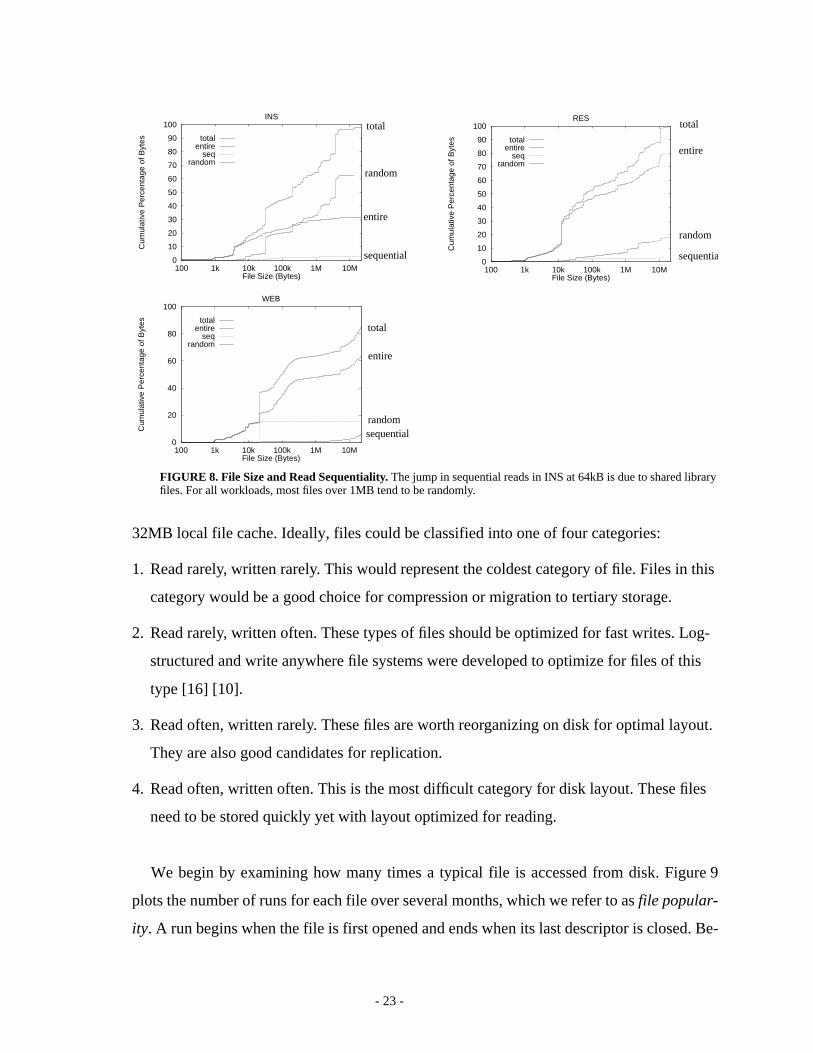
File read access patterns versus file size is shown in Figure 8. The graph for the RES

workload has the same shape as the INS workload. Files that are less than 20kB are typically

0

10

20

30

40

50

60

70

80

90

100

100 1k 10k 100k 1M 10M

Cum

ulat

ive

Per

cent

age

of F

iles

Dynamic File Size (Bytes)

insres

web

FIGURE 7. File Size.The graph of the left shows dynamic file size, which counts the file size of all accessed fileswhen they are closed. The jump in the RES graph at 70kB is due to a repeatedly accessed shared library. The figureon the right shows unique file size. Each unique file is only counted once in this graph.

0

20

40

60

80

100

100 1k 10k 100k 1M 10M

Cum

ulat

ive

Per

cent

age

of F

iles

Unique File Size (Bytes)

insres

web

- 22 -

read in their entirety. For all workloads, large files tend to be read randomly. For the INS and

RES workloads, 33% of the randomly read bytes are library files, 12% are mail files, 11%

are Netscape files, and 13% are temporary files (not including those in the previous catego-

ries).

Most file systems are designed to provide good performance for sequential access to files.

Prefetching strategies often simply prefetch blocks of files that are being accessed sequen-

tially. This provides little benefit to small files since there will not be many blocks to

prefetch. If large files tend to be accessed randomly, this prefetching scheme will prove in-

effective for large files as well, so more extensive prefetching techniques are necessary.

Without effective prefetching, the increasing number of randomly read files may result in

poor file system response time. Mail and web browser applications often access files random-

ly. A boom of new computer users employ mainly these applications; some internet service

providers only provide mail and web browsing services. Traditional file systems are unlikely

to perform satisfactorily under these circumstances.

4.5 File Popularity

In order to study disk layout policies, we are interested in the long-term access patterns

and lifetimes of files stored on disk. In this section, we examine only files that miss in a

TABLE 4. File Access Patterns

A comparison of access patterns across workloads indicates that a larger percentage of files are read randomly in the INS, RES, andWEB workloads than in the Sprite or BSD studies.

INS RES WEB Sprite BSD

Read Percent Runs Entire 71.2 45.6 68.8 68.6 43.2

Percent Runs Sequential 10.0 20.6 22.0 16.7 15.4

Percent Runs Random 17.6 20.3 8.7 2.6 5.2

Write Percent Runs Entire 0.9 1.5 0.3 7.4 22.7

Percent Runs Sequential 0.2 0.3 0.1 3.2 4.7

Percent Runs Random 0.0 0.1 0 0.4 0.9

Read-Write Percent Runs Entire 0.0 0.0 0 0 0

Percent Runs Sequential 0.3 0.7 0.2 0 2.0

Percent Runs Random 0.0 10.9 0 1.0 5.9

- 23 -

32MB local file cache. Ideally, files could be classified into one of four categories:

1. Read rarely, written rarely. This would represent the coldest category of file. Files in this

category would be a good choice for compression or migration to tertiary storage.

2. Read rarely, written often. These types of files should be optimized for fast writes. Log-

structured and write anywhere file systems were developed to optimize for files of this

type [16] [10].

3. Read often, written rarely. These files are worth reorganizing on disk for optimal layout.

They are also good candidates for replication.

4. Read often, written often. This is the most difficult category for disk layout. These files

need to be stored quickly yet with layout optimized for reading.

We begin by examining how many times a typical file is accessed from disk. Figure 9

plots the number of runs for each file over several months, which we refer to asfile popular-

ity. A run begins when the file is first opened and ends when its last descriptor is closed. Be-

0

10

20

30

40

50

60

70

80

90

100

100 1k 10k 100k 1M 10M

Cum

ulat

ive

Per

cent

age

of B

ytes

File Size (Bytes)

INS

totalentire

seqrandom

0

10

20

30

40

50

60

70

80

90

100

100 1k 10k 100k 1M 10M

Cum

ulat

ive

Per

cent

age

of B

ytes

File Size (Bytes)

RES

totalentire

seqrandom

0

20

40

60

80

100

100 1k 10k 100k 1M 10M

Cum

ulat

ive

Per

cent

age

of B

ytes

File Size (Bytes)

WEB

totalentire

seqrandom

FIGURE 8. File Size and Read Sequentiality.The jump in sequential reads in INS at 64kB is due to shared libraryfiles. For all workloads, most files over 1MB tend to be randomly.

sequential sequentia

sequential

entire

entire

entire

random

random

random

total total

total

- 24 -

cause we are interested in disk access patterns, we only count runs that were not absorbed by

the cache.

For WEB, nearly all accesses are reads. Considering this trace is only 3.5 weeks long, a

large number of files are read from disk multiple times. Clearly, this workload would benefit

from a disk layout policy optimized for reads.

For INS and RES, the most popular files (those that are accessed thousands of times) fall

into the category of written often and read rarely. The spike at 1–4 thousand opens for RES

is caused by accesses to system memory log files and mail queue files. The accesses to the

memory log files happen on about half of the hosts and is likely the result of an operating

system bug that the other hosts had patches for. Files that are accessed less frequently tend to

have more read runs than write runs. However, the read to write ratio is low which makes

disk layout difficult since a file that is read one to three times for every time it is written re-

FIGURE 9. File popularity. In these stacked bar graphs, the darkly-colored bottom box shows the number of writeonly runs. The center lightly-colored boxes show the number of read only runs. The top box shows the number of runthat included both reads and writes. The striped boxes to the right of the stacked boxes show the percentage of the totaruns were deleted. This data is based on 3.5 months of traces for INS and RES and 3.5 weeks of traces for WEB.

100k

200k

300k

1 4 16 64 256 1k 4k 16k

Num

ber

of D

isk

Run

s

Number of Disk Runs per File

RES

256k

0

200k

400k

600k

Num

ber

of D

isk

Run

s

Number of Disk Runs per File

WEB

1 4 16 64 256 1k 4k 16k

0

200k

400k

600k

800k

1M

1.2M

1.4MN

umbe

r of

Dis

k R

uns

Number of Disk Runs per File

INS

1 4 16 64 256 1k 4k 16k 256k

- 25 -

quires good performance for both reads and writes. For both of these workloads, many files

are accessed only once. Some of these may be the first reads to files that remain in the cache.

We want to distinguish between two access patterns: files that are accessed infrequently

and files that do not live long enough to be accessed many times. Figure 9 includes an esti-

mate of the number of runs of each category to files that were deleted during the trace. For

each category, the number of deleted runs is estimated by multiplying the total number of

runs by the number of files deleted. The percentage of files deleted decreases with the number

of runs.

In summary, files from the WEB workload are easily classified into the read often, written

rarely category. Reorganizing disk layout for read performance is likely to prove worthwhile.

The INS and RES workloads are less straightforward. Their files display a trimodal distribu-

tion. The high number of files accessed from disk only once may be a combination of reads

to files as they are first faulted into the cache and writes to files that are soon deleted. Files

accessed more times may make disk layout difficult since they are written frequently com-

pared with the number of times they are read. The most highly accessed files are written often

and read rarely. These files would be best supported by a log-style disk layout policy. Ac-

commodating all these access patterns may require an adaptive disk layout policy.

5 Conclusions

The goal of this project is to provide insight into file system traffic in order to aid file sys-

tem design. Some of the clues our analysis suggest include:

1. File systems cannot rely solely on large caches to provide good read performance. The

file system must also use prefetching or disk layout optimized for reads.

2. Block lifetime for our traces is significantly longer than 30 seconds. Write delay alone is

not enough to throttle disk write traffic. File systems will need to use more aggressive

strategies, such as reliable memory or disk logging.

- 26 -

3. Large files are becoming increasingly large and many accesses to large files are nonse-

quential. This decreases the efficacy of simple per-file prefetching techniques used by

many file systems.

4. Read and write access patterns vary among files. To provide good performance, disk lay-

out policies may need to change layout strategies depending on each file’s access pat-

terns.

Clearly, our results have only scratched the surface of the possible studies enabled by hav-

ing detailed, long-term traces. Our future work includes more studies than can be reasonably

enumerated here.

Acks

Trace collection was accomplished with the support of many of Berkeley’s technical staff.

Francisco Lopez provided invaluable assistance as the local HP-UX guru and main technical

support contact for the instructional cluster; Eric Fraser created the infrastructure for the trace

collection host; Kevin Mullally, Jeff Anderson-Lee, Ginger Ogle, Monesh Sharma, and

Michael Short contributed to the installation and testing of the trace collection process. Fran-

cisco Lopez, Ginger Ogle, and Joyce Gross provided insight into the analysis of system ac-

tivity.

Jeanna Matthews, Steve Lumetta, and Thomas Kroeger provided valuable feedback on

this work, and Eric Anderson waded through numerous iterations of this paper.

Nacks

Finally, the authors would like to nack several people who knew how difficult this would

be but allowed me to do it anyway. You know who you are.

References

[1] M. Baker, J. Hartman, M. Kupfer, K. Shirriff, and J. Ousterhout, “Measurements of aDistributed File System,”ACM 13th Symposium on Operating Systems Principles, pp.198–212, 1991.

- 27 -

[2] P. Chen, E. Lee, G. Gibson, R. Katz, and D. Patterson, “RAID: High-Performance, Re-liable Secondary Storage,”ACM Computing Surveys, 26(2):145-188, June 1994.

[3] P. Chen, W. Ng, S. Chandra, C. Aycock, G. Rajamani, D. Lowell, “The Rio File Cache:Surviving Operating System Crashes,”ASPLOS VII, pp. 74–83, October 1996.

[4] Dahlin, Michael, Randy Wang, Thomas Anderson, and David Patterson, “A QuantitativeAnalysis of Cache Policies for Scalable Network File Systems,”Proceedings of the1994 SIGMETRICS, pp. 150–160, May 1994.

[5] M. Dahlin, R. Wang, T. Anderson, and D. Patterson, “Cooperative Caching: Using Re-mote Memory to Improve File System Performance,”Proceedings of the First Sympo-sium on Operating Systems Design and Implementation, pp. 267-280, November 1994.

[6] M. Feeley, W. Morgan, F. Pighim, A. Karlin, H. Levy, and C. Thekkath, “ImplementingGlobal Memory Management in a Workstation Cluster,”Proceedings of the FifteenthACM Symposium on Operating Systems Principles, pp. 201-212,December 1995.

[7] D. Ghormley, D. Petrou, S. Rodrigues, and T. Anderson, “SLIC: An Extensibility Sys-tem for Commodity, Operating Systems”USENIX Technical Conference, June 1998.

[8] S. Gribble, G. Manku, D. Roselli, E. Brewer, T. Gibson, and E. Miller, “Self-Similarityin File Systems,Proceedings of ACM SIGMETRICS 1998, Madison, Wisconsin, June1998.

[9] J. Hartman, J. Ousterhout, “The Zebra Striped Network File System,”ACM Transac-tions on Computer Systems, vol. 13, no. 3, August 1995, pp. 279-310, August 1995.

[10] D. Hitz, J. Lau, and M. Malcom, “File System Design for an NFS File Server Appli-ance,” Network Appliance Technical Report TR3002, March 1995.

[11] J. Howard, M. Kazar, S. Menees, D. Nichols, M. Satyanarayanan, R. Sidebotham, andM. West. “Scale and Performance in a Distributed File System”,ACM Transactions onComputer Systems, 6(1):51-81, February, 1988.

[12] M. Mckusick, W. Joy, S. Leffler, and R. Fabry, “A Fast File System for UNIX,”ACMTransactions on Computer Systems, vol. 2, no. 3, pp. 181-197, August 1984.

[13] L. Mummert and M. Satyanarayanan, “Long Term Distributed File Reference Tracing:Implementation and Experience,” SP&E 26(6): pp. 705-736, 1996.

[14] J. Ousterhout, H. Da Costa, D. Harrison, J. Kunze, M. Kupfer, and J. Thompson, “ATrace-Driven Analysis of the UNIX 4.2 BSD File System,”ACM 10th Symposium onOperating Systems Principles, pp. 15-24, 1985.

[15] E. Riedel and G. Gibson, “Understanding Customer Dissatisfaction with Underutilized

- 28 -

Distributed File Servers,”Proceedings of the 5th NASA Goddard Space Flight CenterConference on Mass Storage Systems and Technologies, September 1996.

[16] M. Rosenblum and J. Ousterhout, “The Design and Implementation of a Log-Struc-tured File System for UNIX,” ACM Transactions on Computer Systems, 10(1):26-52,February 1992.

[17] C. Ruemmler and J. Wilkes, “UNIX Disk Access Patterns,”Proceedings of Winter US-ENIX 1993, CA, January 1993.

[18] Seagate, 1998. Data sheet for the Cheetah9LP, http://www.seagate.com/disc/cheetah/cheetah.shtml.

[19] K. Smith and M. Seltzer, “File Layout and File System Performance,” Harvard Techni-cal Report TR-35-94, 1994.

[20] A. Sweeney, D. Doucette, W. Hu, C. Anderson, M. Nishimoto, and G. Peck, “Scalabil-ity in the XFS File System,”Proceedings of the USENIX 1996 Technical Conference,January, 1996.

[21] M. Wittle and B. Keith, “LADDIS: The Next Generation in NFS File Server Bench-marking,”Proceedings of Summer USENIX, pp. 111-128, June 1993.

- 29 -

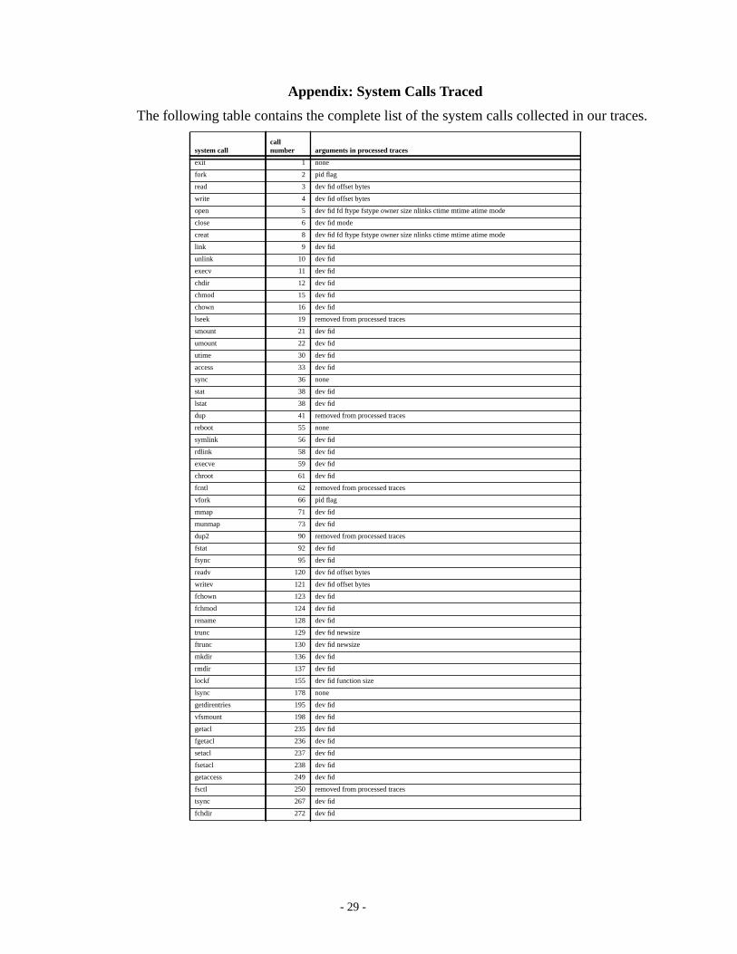
Appendix: System Calls Traced

The following table contains the complete list of the system calls collected in our traces.

system callcallnumber arguments in processed traces

exit 1 none

fork 2 pid flag

read 3 dev fid offset bytes

write 4 dev fid offset bytes

open 5 dev fid fd ftype fstype owner size nlinks ctime mtime atime mode

close 6 dev fid mode

creat 8 dev fid fd ftype fstype owner size nlinks ctime mtime atime mode

link 9 dev fid

unlink 10 dev fid

execv 11 dev fid

chdir 12 dev fid

chmod 15 dev fid

chown 16 dev fid

lseek 19 removed from processed traces

smount 21 dev fid

umount 22 dev fid

utime 30 dev fid

access 33 dev fid

sync 36 none

stat 38 dev fid

lstat 38 dev fid

dup 41 removed from processed traces

reboot 55 none

symlink 56 dev fid

rdlink 58 dev fid

execve 59 dev fid

chroot 61 dev fid

fcntl 62 removed from processed traces

vfork 66 pid flag

mmap 71 dev fid

munmap 73 dev fid

dup2 90 removed from processed traces

fstat 92 dev fid

fsync 95 dev fid

readv 120 dev fid offset bytes

writev 121 dev fid offset bytes

fchown 123 dev fid

fchmod 124 dev fid

rename 128 dev fid

trunc 129 dev fid newsize

ftrunc 130 dev fid newsize

mkdir 136 dev fid

rmdir 137 dev fid

lockf 155 dev fid function size

lsync 178 none

getdirentries 195 dev fid

vfsmount 198 dev fid

getacl 235 dev fid

fgetacl 236 dev fid

setacl 237 dev fid

fsetacl 238 dev fid

getaccess 249 dev fid

fsctl 250 removed from processed traces

tsync 267 dev fid

fchdir 272 dev fid

- 30 -

General Notes on Arguments

Most calls have the argumentsdev andfid, where dev is the device number of the file sys-

tem and fid is a unique file identifier on that system.

Special Notes on Arguments

fork , vfork — have two arguments: a process identifier and a flag which is nonzero if

this is the child. If this is the child, the first argument is the parent’s process id. If this is the

parent, the first argument is the child’s process id.

open , creat — have ten arguments in addition to the dev and fid.Fd is the file descrip-

tor returned by the call,ftype is the file type (regular, directory, symbolic link, or empty di-

rectory),fstype is the type of file system (local or NFS),owner is the user id of the file’s

owner,size is the file size in bytes,nlinks is the number of hard links,ctime, mtime, andatime

refer to the last change time, modify time and access time respectively, andmode is the open/

create mode.

close — mode indicates whether this is the final close for this file.