Characteristics of Refrigerant Film Thickness, Pressure Drop, and Heat

Transfer in Annular Flow

ACRC TR-110

For additional information:

Air Conditioning and Refrigeration Center University of Illinois Mechanical & Industrial Engineering Dept. 1206 West Green Street Urbana. IL 61801

(217) 333-3115

E. T. Hurlburt and T. A. Newell

February 1997

Prepared as part of ACRC Project 71 Two-Phase Modeling of Refrigerant and Refrigerant-Oil

Mixtures Over Enhanced/Structured Surfaces T. A. Newell, Principal Investigator

The Air Conditioning and Refrigeration Center was founded in 1988 with a grant from the estate of Richard W. Kritzer, the founder of Peerless of America Inc. A State of Illinois Technology Challenge Grant helped build the laboratory facilities. The ACRC receives continuing support from the Richard W. Kritzer Endowment and the National Science Foundation. The following organizations have also become sponsors of the Center.

Amana Refrigeration, Inc. Brazeway, Inc. Carrier Corporation Caterpillar, Inc. Copeland Corporation Dayton Thermal Products Delphi Harrison Thermal Systems Eaton Corporation Ford Motor Company Frigidaire Company General Electric Company Hydro Aluminum Adrian, Inc. Lennox International, Inc. Modine Manufacturing Co. Peerless of America, Inc. Redwood Microsystems, Inc. The Trane Company Whirlpool Corporation

For additional information:

Air Conditioning & Refrigeration Center Mechanical & Industrial Engineering Dept. University of Illinois 1206 West Green Street Urbana IL 61801

2173333115

Characteristics of Refrigerant Film Thickness, Pressure Drop, and Heat Transfer in Annular Flow

Evan T. Hurlburt and Ty A. Newell

Abstract

Common refrigeration and air conditioning cycles are dependent on two-phase flow for

efficient heat transfer with minimal pressure drop. Design of heat exchangers for these systems is

aided by an understanding of the refrigerant pressure drop and local heat transfer coefficient. An

estimate of the liquid fraction is also important for predicting the charge required in a system. The

present work develops a semi-analytical model for predicting liquid fraction, pressure drop, and

heat transfer for pure refrigerants in the annular flow regime. The model uses the approach of

coupling a uniformly thick, turbulent liquid film layer with a turbulent vapor core. Model

predictions are compared to experimental evaporation and condensation data for Rll, R12, R134a,

and R22. These refrigerants represent the low, medium, and high pressure ranges found in

common refrigeration systems. The uniform film model, when compared to experimental data,

provides a reference for understanding some of the mechanisms that are important to refrigerant

two-phase flow.

Introduction

The refrigeration and air conditioning industry has historically been interested in two-phase

flow, however, a renewed interest in understanding two-phase flow from a more fundamental

basis has developed over the past decade as new candidate refrigerant compounds are examined.

Conversion from common refrigerants to lesser known compounds causes significant concern

among manufacturers in terms of system performance, reliability, liability, and consumer

acceptance. Continued research into two-phase flow related to refrigerants will continue to be

important in order to model and design "enhanced" surfaces, determine the effects and predict the

movement of lubricating oil in refrigerant vapor lines, and predict the effects of zeotropic

refrigerant mixtures that may offer performance advantages. Characteristics of pressure drop, heat

transfer, and void fractions of common refrigerants are modeled and compared to experimental data

in this study. The semi-analytical modeling approach used is helpful for understanding physical

processes that are important over the annular flow region of interest to refrigeration systems.

1

Environmental concerns have created significant interest in understanding two-phase flow

phenomena in the air conditioning and refrigeration community. Two driving forces are ozone

depletion and global warming. Ozone depletion concerns have resulted in the phase out of fully

halogenated compounds containing chlorine (CFCs). RII (CCI3F) and R12 (CC12F2) are two

examples of common refrigerants that have been phased out. New refrigeration equipment using

partially halogenated compounds containing chlorine, called HCFCs, will not be manufactured

after 2010. R22 (CHC1F2) is an HCFC that is commonly used for household air conditioning

systems.

Global warming is a concern that has affected the refrigeration industry in two ways. First,

many refrigerant compounds are strong absorbers of infrared radiation. When a refrigerant is

released into the atmosphere, a "direct" contribution to global warming is realized. R134a

(CF3CH2F), the common replacement for R12 systems, has a 100 year Global Warming Potential

(GWP) of 1200. This represents the amount of carbon dioxide that would cause the same level of

infrared radiation absorption as a unit mass of the refrigerant over a 100 year period. GWPs range

from 100 to 5000 for most compounds of interest for refrigeration (DOE (1993».

The second effect relevant to global warming is called the "indirect" effect. Energy

consumption in general, may require combustion of fossil fuels with the resulting release of carbon

dioxide. Coal produces a significant amount of carbon dioxide relative to natural gas on an

equivalent energy basis. Renewable energies (hydropower, solar energy, wind energy) and

nuclear energy are examples of processes that result in negligible production of carbon dioxide.

From the viewpoint of a refrigeration equipment manufacturer, reducing the indirect effect requires

improving a component's energy efficiency. A U.S. refrigerator manufactured in 1970 produced

21,000 kg of carbon dioxide over its lifetime from both direct and indirect effects. Direct effects

from the release of refrigerant compounds accounted for 25 percent of this amount. A U.S.

refrigerator manufactured after 1995 can expect to have an equivalent carbon dioxide output of

6500 kg. Approximately 1000 kg of carbon dioxide is due to the direct effect of the new

replacement refrigerant compounds (if not reclaimed) and the remaining portion is due to the

indirect effect of a unit's electrical energy consumption (Newell (1996».

Background

A wide range of operating conditions and system capacities have resulted in a relatively wide

variety of substances used as refrigerants. The present paper focuses on halocarbon refrigerants

that are derivatives of methane and ethane. Combinations of fluorine, chlorine, and hydrogen atom

arrangements on these one-carbon and two-carbon molecules leads to a large range of properties

that are significantly different from properties of saturated steam or air-water two-phase flow

properties. While several correlation models exist for common refrigerants, significant uncertainty

2

exists when highly empirical correlations are used to model new refrigerant candidates. In

addition, purely empirical correlations, while employing physically derived parameter groups, do

not allow a more refined examination of the details of the flow field.

Table 1 shows density, viscosity, and thermal conductivity data for R22, R134a, and R123

refrigerants relative to air-water. The refrigerant data show saturated liquid and vapor properties at

two temperatures that represent variations one may expect to find between the condenser and

evaporator of a refrigeration system. R22 is an example of a "high pressure" refrigerant. The high

pressure results in relatively high vapor densities. R134a is typical of a medium pressure range

compound while R123, one replacement for Rll, is a "low pressure" refrigerant that is often

working at pressures less than atmospheric pressure. Figure 1 is a schematic showing the range of

mass fluxes and heat fluxes that are characteristic of refrigerants for common household

applications. Also plotted on Figure 1 are areas that represent validity ranges of some commonly

used correlations for two-phase refrigerant flows (Jung and Radermacher (1991), Kandlikar

(1990), Pierre (1956), Shah (1976». Common tube diameters for these refrigeration systems

range from 3 mm to 10 mm. Significant activity is occurring with microchannels for refrigeration

systems where tube passageways are less than 1 mm in diameter (Huen (1995) and Zietlow

(1995». These systems tend to be in a range where surface tension effects are significant.

Table 1 Comparison of saturation properties for R22, R134a, and R123 to air-water. R22, R134a, and R123 data taken from Gallagher, et ale (1993). Air and water data taken from Incropera and DeWitt (1985).

R22 vapor (00 C) R22 liquid (00 C) R22 vapor (400 C) R22 liquid (400 C) R134a vapor (00 C) R134a liquid (00 C) R134a vapor (400 C) R134a liquid (400 C) Rl23 vapor (00 C) R123 liquid (00 C) R123 vapor (400 C) R123 liquid (400 C) Air (200 C) Water (101 kPa, 200 C)

pressure (kPa) 497.7 497.7 1538. 1538. 292.2 292.2 1018. 1018. 32.65 32.65 154.3 154.3 101.3 101.3

density (kglm3)

21.11 1279. 65.72 1127. 14.23 1294. 49.09 1144. 2.24

1522. 9.59

1423. 1.23

1001.

3

viscosity (mpoise)

117.2 2205. 141.9 1424. 109.4 2857. 131.0 1775. 96.0

5920. 111.1 3623.

1.8 10000.

thermal conductivity (W/m-K) 0.0100 0.1034 0.0126 0.0793 0.0119 0.0939 0.0155 0.0736 0.0083 0.0858 0.0104 0.0743

0.026 0.60

100

-. N e ~ 10 ~ .c::r ~ =' ti: 1 ~

~

0.1 10 000 1

Mass Flux, G (kglmA2-s)

Figure 1 Map of heat flux versus mass flux showing range of applicability of various correlations and operation ranges of refrigerators, room air conditioners, and residential heat pumps.

Fluid Flow and Film Thickness Modeling

In developing a model that predicts refrigerant heat transfer, the physics of the flow field in

both the liquid and vapor phases must first be addressed. While flowing through an evaporator or

condenser, a refrigerant passes through a series of different two-phase flow regions. For example,

in the evaporator there is a relatively large fraction of liquid at the entrance. In a horizontal tube

this results in either a slug flow or stratified-wavy flow pattern with most of the liquid flowing on

the tube bottom and vapor flowing in the space above the liquid.

At constant total mass flow rate, as the liquid fraction decreases, vapor velocity increases. If

the vapor velocity is high enough, the flow pattern will transition to annular flow. In annular flow,

the fluid flows in a thin [:tIm on the tube wall with the vapor flowing in the core created by the

liquid boundary. If the liquid Reynolds number is high enough, periodic collections of waves,

. called disturbance waves, will form. A fraction of the liquid phase flows in the vapor core in the

form of droplets. At high refrigerant quality, the flow field transitions to mist flow in which the

liquid phase is carried along primarily as droplets in the vapor (Whalley (1987), Carey (1992».

At moderate to high refrigerant mass flux and in tubes of hydraulic diameter from 3 mm to 10

mm in diameter, the predominant flow pattern in both the evaporator and condenser is annular

flow. This was demonstrated by Wattelet (1994) for evaporator tubes with inner diameters of 7.04

mm, 7.75 mm, 10.21 mm, and 10.92 mm. Annular flow was observed in all four tubes at mass

fluxes above 200 kg/m2-s over the quality range of 0.2 < x < 0.9.

4

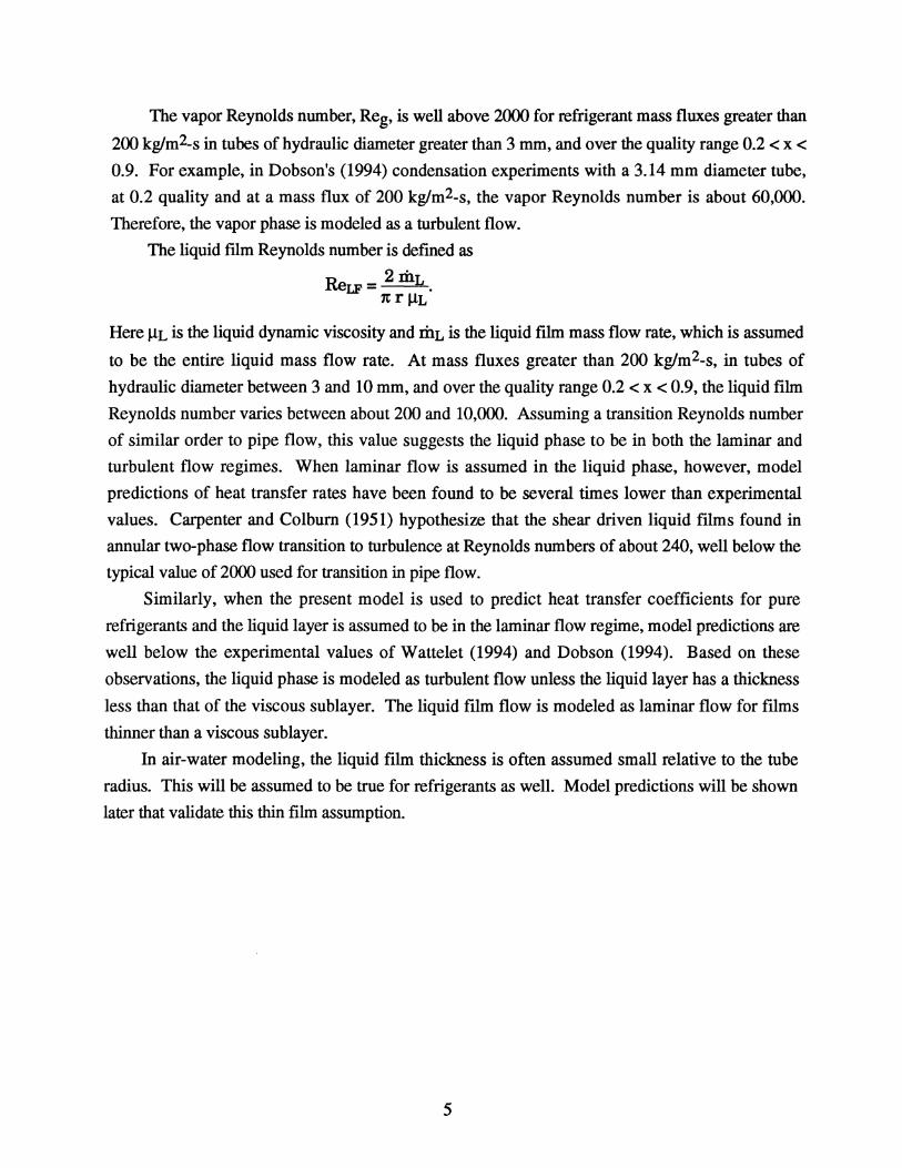
The vapor Reynolds number, Reg, is well above 2000 for refrigerant mass fluxes greater than

200 kg/m2-s in tubes of hydraulic diameter greater than 3 mm, and over the quality range 0.2 < x < 0.9. For example, in Dobson's (1994) condensation experiments with a 3.14 mm diameter tube,

at 0.2 quality and at a mass flux of 200 kg/m2-s, the vapor Reynolds number is about 60,000.

Therefore, the vapor phase is modeled as a turbulent flow.

The liquid ftlm Reynolds number is defined as

ReLF = 2 rilL • 1t r J.1L

Here J.1L is the liquid dynamic viscosity and rilL is the liquid film mass flow rate, which is assumed

to be the entire liquid mass flow rate. At mass fluxes greater than 200 kg/m2-s, in tubes of

hydraulic diameter between 3 and 10 mm, and over the quality range 0.2 < x < 0.9, the liquid film

Reynolds number varies between about 200 and 10,000. Assuming a transition Reynolds number

of similar order to pipe flow, this value suggests the liquid phase to be in both the laminar and

turbulent flow regimes. When laminar flow is assumed in the liquid phase, however, model

predictions of heat transfer rates have been found to be several times lower than experimental

values. Carpenter and Colburn (1951) hypothesize that the shear driven liquid films found in

annular two-phase flow transition to turbulence at Reynolds numbers of about 240, well below the

typical value of 2000 used for transition in pipe flow.

Similarly, when the present model is used to predict heat transfer coefficients for pure

refrigerants and the liquid layer is assumed to be in the laminar flow regime, model predictions are

well below the experimental values of Wattelet (1994) and Dobson (1994). Based on these

observations, the liquid phase is modeled as turbulent flow unless the liquid layer has a thickness

less than that of the viscous sublayer. The liquid film flow is modeled as laminar flow for films

thinner than a viscous sublayer.

In air-water modeling, the liquid film thickness is often assumed small relative to the tube

radius. This will be assumed to be true for refrigerants as well. Model predictions will be shown

later that validate this thin ftlm assumption.

5

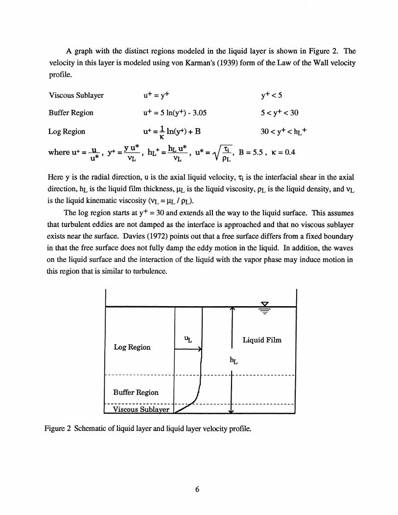
A graph with the distinct regions modeled in the liquid layer is shown in Figure 2. The

velocity in this layer is modeled using von Karman's (1939) form of the Law of the Wall velocity

profile.

Viscous Sublayer

Buffer Region

Log Region

u+=y+

u+ = 5 In(y+) - 3.05

u+ = lIn(y+) + B K

5 < y+ < 30

where u+ = ~, y+ = y u* , hL + = hL u* , u* = . (ii, B = 5.5, K = 0.4 u* VL VL 1V PZ

Here y is the radial direction, u is the axial liquid velocity, 'ti is the interfacial shear in the axial

direction, hL is the liquid film thickness, ilL is the liquid viscosity, PL is the liquid density, and VL

is the liquid kinematic viscosity (VL = ilL / pL).

The log region starts at y+ = 30 and extends all the way to the liquid surface. This assumes

that turbulent eddies are not damped as the interface is approached and that no viscous sublayer

exists near the surface. Davies (1972) points out that a free surface differs from a fixed boundary

in that the free surface does not fully damp the eddy motion in the liquid. In addition, the waves

on the liquid surface and the interaction of the liquid with the vapor phase may induce motion in

this region that is similar to turbulence.

v --

uL Liquid Film Log Region .... ,

hL

------------------ ------- -------- -----------------

Buffer Region

~--------------------------- -----------------Viscous Sublayer

Figure 2 Schematic of liquid layer and liquid layer velocity profile.

6

Extending the Log Law to the liquid surface, the interface velocity, Uj, can be found by

evaluating the Log Region profIle at hL .

.!!i..= Lln(hL +) + B u* K

where hL + = hL u* ,u* = . TiL , and B = 5.5 VL 'V "Pr.

(1)

Another useful relation can be found by integrating the Law of the Wall velocity profIle. The

liquid mass flux for a uniform thin fIlm is defined as

UL, ... Ae = 2 "r fL U ely, (2)

where Ac = 1t r hL and UL,avg is the average liquid velocity in the axial direction. With the velocity

profile a known function of the film thickness and shear stress, integration relates these to the

average liquid velocity.

UL,avg = l.ln(hL +) + B _1. _ 64 u* K K hL+ (3)

where u* = . Iii 'V"Pr.

When the liquid layer reaches a non-dimensional film thickness less than 30 ( hL + < 30), the

approach taken in modeling the liquid phase is to use the unmodified Law of the Wall velocity

profile. An alternative approach would be to scale the viscous sublayer, buffer region, and log

region boundaries, thus keeping intact a sub layer to turbulent region characteristic. Scaling of the

boundaries has not been found to offer a clear advantage and has therefore not been used. When

hL + is less than 5, the liquid flow is modeled as laminar flow. In a uniform ftIm thickness model,

this condition is only reached at very high quality.

The vapor phase Reynolds number, for the flow conditions of interest, is always high enough

to result in a turbulent flow. The vapor velocity profile, therefore, can be modeled using the Law

of the Wall velocity profile with the friction velocity evaluated using the interfacial shear stress.

No viscous sublayer or buffer regions are assumed to be present in the vapor.

Integrating the log law from 0 to r-hL to determine the average vapor velocity gives the

following equation,

Ug,avg - Ui = 1. lJ (r - hL) Us *] + B _ ~ us* K .&1.1 Vg 2 K

(4)

where Us* = . K "If);

7

Here, Ug,avg - Ui is the average vapor velocity relative to the liquid film interface, 'ts is the smooth

tube vapor wall shear stress, Pg is the vapor density, r - hL is the radius of the vapor core, and Vg

is the kinematic viscosity of the vapor (Vg = J.Lg I pg, where J.Lg is the vapor viscosity). Equation

(4) predicts values identical to the smooth-tube friction factors in the Moody chart. It is an

approximation since its derivation assumes the entire velocity profIle to be described by the Log

Law. The error is, however, negligible since nearly all the mass is in the Log Region when the

Reynolds number is much greater than 2000.

The vapor core in annular two-phase flow is driven by the pressure gradient in the tube. The

liquid fIlm, however, is driven primarily by momentum transfer from the vapor. This momentum

transfer is very large resulting in high shear stress in the liquid fIlm and from 2 to 10 times higher

pressure drop than is found in smooth tube single-phase flow (Asali, et al. (1985)).

A detailed accounting of the momentum transfer requires modeling of the complex interaction

between the liquid surface waves and the vapor flow field. An alternate approach is to represent

the momentum exchange by an average interfacial shear stress, 'ti. In the modeling to date, both a

momentum exchange model and a prediction based on a correlation have been attempted. The

momentum exchange model provides a conceptual guide to help understand the transfer. The

correlation-base approach is presented in this work.

The correlation used to predict the interfacial shear is a modified form of the correlation

developed by Asali, et al. (1985) for vertical flow.

'ti _ 1 = 0.45 Reg-O.3 (eI> hL + - 4) (5) 'ts

J.LL {pg)O.5 h + _ hL u* * _ {fi d Re _ pg (ug,avg - Ui) (r - hd where eI> = - - ,L - , U - - ,an g - ..:....=---=---=-----J.Lg PL VL PL J.Lg

The smooth tube shear, 'ts, can be found from equation (4), and it is the limiting value reached as

the [11m thickness tends toward zero.

In the original form of equation (5) proposed by Asali, et al. (1985), the exponent on the

vapor phase Reynolds number, Reg, is -0.2. The value of -0.3 is used to improve the match

between the model predictions and Wattelet's (1994) R134a experimental data for pressure drop.

Figure 3 shows a comparison between the data and model predictions for three mass fluxes over a

range of quality. Model predictions with the vapor phase Reynolds number equal to -0.2 is

included for comparison.

8

80

70

...... • 60 =-..1/1 .....

"" 50

0 ... ~ 40 GI ... :I

30 .. .. GI ...

=- 20

10

0

o Wattelet - A

[J Wattelet - B

11 Wattelet - C

2 A = 200 kg/m -8

B = 300 kg 1m2 - 8 ...... +.-----------------------2 !

C = 500 .k g 1m - 8 . _______ ~-------------------------: .. ---- .. : ... - : ...

-Model - Re -0.3 (A.B,C) # 1 i " g -----,-""------r----------------------------r---------'-:-----------

- -- -Model - Re -0.2 (A.B,C)' i i g "

I'----------------------------------."!"""j--------~---:--,--'---~--~.'I---~....I.=r-=+== .... -.... -................ ~.# ...................... ~.-... ·::·:·:·,::·;;--·-·-·-·-·f·:.;·;·:-~···u_--.. .

1 ... -i--- i [] i Cl .......................... . .......... --...... ~--................ -.... --... ~ ........................................................... . f-.--- : ---- :--0----: --c'

0 0_2 0.4 0.6 0_8

Quality

Figure 3 Comparison of model pressure drop predictions with evaporator data for R134a from Wattelet (1994). Model predictions are at two different values of the exponent on the Reynolds number in the interfacial shear correlation. (Horizontal D = 7.75 mm L = 1.22 m T = 50 C)

Film Thickness Predictions

Equations (1), (3), (4), and (5), can be solved simultaneously at a specified liquid and vapor

mass flow rate, tube radius, and refrigerant temperature to predict the thickness of the liquid ftIm.

Figure 4 shows this prediction for R-134a at three different mass fluxes over the quality range 0.2

< x < 0.9. Note how thin the film is at high quality (less than 0.2 mm for the chosen range of

mass fluxes). Note, also, that the radius is at least 8 times greater than the film thickness at the

lowest quality. At higher qualities it is more than 20 to 50 times greater. This is consistent with

the thin film assumption.

It is interesting that the ftIm is predicted to become progressively thinner as the total mass flux

increases. This is due to the increased shear from the vapor. The higher average vapor velocity

increases the average liquid film velocity allowing a higher flux through a smaller cross sectional

area.

9

i e ......

0.5~--~A--~------~i------~---2----~1 ------~

i A =200 kg/m -8 ! i 2 i

0.4 .............. ~ .. ~ .................... + ..... ~:::: ::::2~: .......... :::.!:.: ......................... . i ~ j

~ ~ ~ 0 .. 3 __ ..................... u •• .;............ ••• ••• • ••• ;. ............................ i-............................ ; ....................... h ••

02'--+--~ .... . I-+-! ! : !

0.1 ··························t····················· .. ···} ......................... -t.......... . i i ! iii f ~ ~

o~------~----~------~------~------~ o 0.2 0.4 0.6 0.8 1

Quality

Figure 4 Prediction of liquid ftIm thickness versus quality for R134a at three mass fluxes. (D = 7.75 mm L = 1.22 m T = 50 C)

The model prediction of the non-dimensional film thickness, hL +, can be compared to the

prediction from the correlations developed by Asali, et al. (1985) and Henstock and Hanratty

(1976).

hL + Correlation = [(0.34 ReL 0.6)2.5 + (0.0379 ReLO.9)2.5]0.4

Table 2 shows this comparison for R-134a at mass fluxes of 200, 300, and 500 kglm2-s and a

temperature of 50 C. The difference between the model and the correlation predictions is never

more than 5%. Although this does not prove the Law of the Wall velocity profile is the actual

prome within the liquid film, the agreement indicates that the Law of the Wall may be a reasonable

means of modeling the film. It is worth noting that R134a has a liquid to vapor density ratio of

approximately 90 while the density ratio of liquid water to air, upon which the interfacial shear

correlation is based, is approximately 800. Note also that although the film thickness decreases

with mass flux, the non-dimensional ftIm thickness increases. This is because the friction velocity

is increasing faster than the mm thickness is decreasing.

10

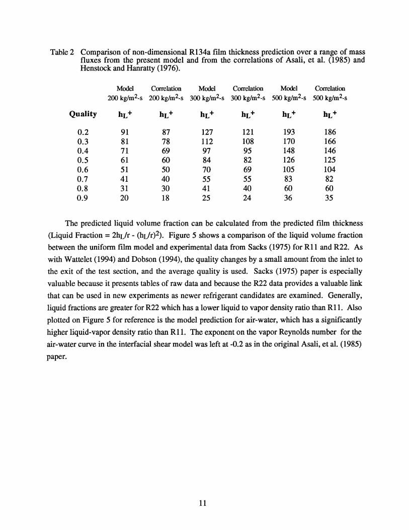
Table 2 Comparison of non-dimensional R134a film thickness prediction over a range of mass fluxes from the present model and from the correlations of Asali, et al. (1985) and Henstock and Hanratty (1976).

Model Correlation Model Correlation Model Correlation 200 kglm2-s 200kgIm2-s 300 kglm2-s 300 kglm2-s 500 kglm2-s 500 kglm2-s

Quality hL+ hL+ hL+ hL+ hL+ hL+

0.2 91 87 127 121 193 186 0.3 81 78 112 108 170 166 0.4 71 69 97 95 148 146 0.5 61 60 84 82 126 125 0.6 51 50 70 69 105 104 0.7 41 40 55 55 83 82 0.8 31 30 41 40 60 60 0.9 20 18 25 24 36 35

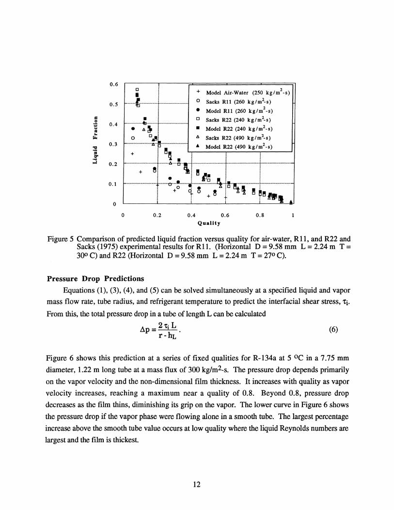
The predicted liquid volume fraction can be calculated from the predicted fIlm thickness

(Liquid Fraction = 2hrJr - (hIJr)2). Figure 5 shows a comparison of the liquid volume fraction

between the uniform film model and experimental data from Sacks (1975) for Rll and R22. As

with Wattelet (1994) and Dobson (1994), the quality changes by a small amount from the inlet to

the exit of the test section, and the average quality is used. Sacks (1975) paper is especially

valuable because it presents tables of raw data and because the R22 data provides a valuable link

that can be used in new experiments as newer refrigerant candidates are examined. Generally,

liquid fractions are greater for R22 which has a lower liquid to vapor density ratio than Rll. Also

plotted on Figure 5 for reference is the model prediction for air-water, which has a significantly

higher liquid-vapor density ratio than Rl1. The exponent on the vapor Reynolds number for the

air-water curve in the interfacial shear model was left at -0.2 as in the original Asali, et al. (1985)

paper.

11

0.6

0.5

o ! I i + Model Air-Water (250 kg/m2_s)

······«··············t······················ : ==:1 ~111 ~2:: ::11:2~~:) = .~ 0.4 .... .. "

• i 0 Sacks R22 (240 kg/m2-s) ............ ~ ........ l ..................... .

• t>. ~ ~ • Model R22 (240 kg/m2-s) a.

f;r;o

0.3 ." .; CI"'

::s 0.2

0.1

0

o D~~ t:. Sacks R22 (490 kg/m2-s) I-····················a··!···················· ... Model R22 (490 kg/m2-s)

+ I ~~. ~ ~ ~ ··········:·········er·····&···u.\l".~ ................. ··r·······················r······················-

i. i ~ i i I-······················+······a···~·······~····;······ ...... ~ .. ].~ .. ~ .............. + ....................... -

i + q. 0 ~ i t:. ~ ~ e!l! i i + t : 11'11 •

o 0.2 0.4 0.6 0.8 Quality

Figure 5 Comparison of predicted liquid fraction versus quality for air-water, Rll, and R22 and Sacks (1975) experimental results for Rii. (Horizontal D = 9.58 mm L = 2.24 m T = 300 C) and R22 (Horizontal D = 9.58 mm L = 2.24 m T = 270 C).

Pressure Drop Predictions

Equations (1), (3), (4), and (5) can be solved simultaneously at a specified liquid and vapor

mass flow rate, tube radius, and refrigerant temperature to predict the interfacial shear stress, 'ti.

From this, the total pressure drop in a tube of length L can be calculated

ilp = 2 'ti L . (6) r-hL

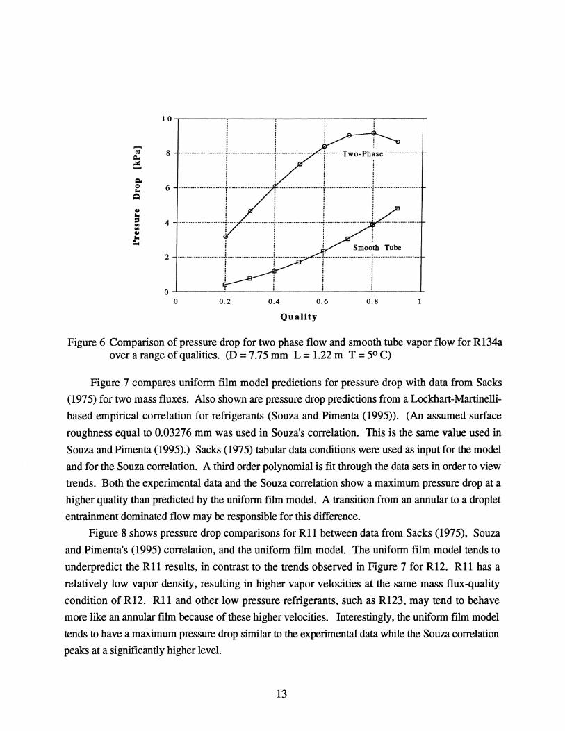
Figure 6 shows this prediction at a series of fixed qualities for R-134a at 5 0C in a 7.75 mm

diameter, 1.22 m long tube at a mass flux of 300 kg/m2-s. The pressure drop depends primarily

on the vapor velocity and the non-dimensional film thickness. It increases with quality as vapor

velocity increases, reaching a maximum near a quality of 0.8. Beyond 0.8, pressure drop

decreases as the film thins, diminishing its grip on the vapor. The lower curve in Figure 6 shows

the pressure drop if the vapor phase were flowing alone in a smooth tube. The largest percentage

increase above the smooth tube value occurs at low quality where the liquid Reynolds numbers are

largest and the film is thickest.

12

10~------~:------~------'-------r------. ! f ! !

8 ··························t·························.: ...............•... ..-t ........ Two-Phase ................... . : : : : i ~ : :

: =::::l:-~:=,=t::[~=:~ . i i

2 ··························t··························1 •...................... ~ ................•......... [ ......................... . : : : : : ::

! I I O~------~----~------~------~------~

o 0.2 0.4 0.6 0.8 1

Quality

Figure 6 Comparison of pressure drop for two phase flow and smooth tube vapor flow for R134a over a range of qualities. (D = 7.75 mm L = 1.22 m T = 50 C)

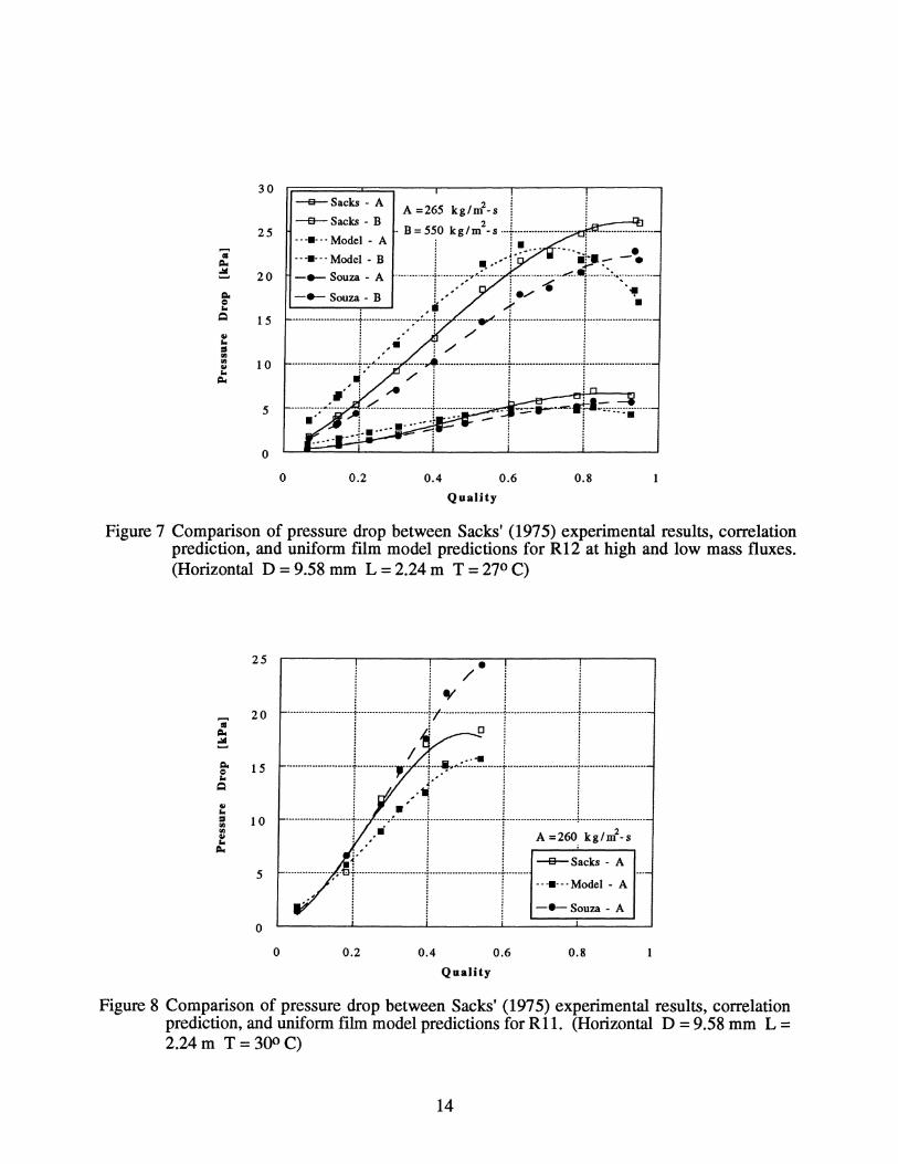
Figure 7 compares uniform film model predictions for pressure drop with data from Sacks

(1975) for two mass fluxes. Also shown are pressure drop predictions from a Lockhart-Martinelli­

based empirical correlation for refrigerants (Souza and Pimenta (1995». (An assumed surface

roughness equal to 0.03276 mm was used in Souza's correlation. This is the same value used in

Souza and Pimenta (1995).) Sacks (1975) tabular data conditions were used as input for the model

and for the Souza correlation. A third order polynomial is fit through the data sets in order to view

trends. Both the experimental data and the Souza correlation show a maximum pressure drop at a

higher quality than predicted by the uniform film model. A transition from an annular to a droplet

entrainment dominated flow may be responsible for this difference.

Figure 8 shows pressure drop comparisons for Rll between data from Sacks (1975), Souza

and Pimenta's (1995) correlation, and the uniform film model. The uniform film model tends to

underpredict the Rl1 results, in contrast to the trends observed in Figure 7 for R12. Rll has a

relatively low vapor density, resulting in higher vapor velocities at the same mass flux-quality

condition of R12. Rll and other low pressure refrigerants, such as R123, may tend to behave

more like an annular fIlm because of these higher velocities. Interestingly, the uniform film model

tends to have a maximum pressure drop similar to the experimental data while the Souza correlation

peaks at a significantly higher level.

13

30 -e-Sacks - A

-e-Sacks - B 25 .. -. ... Model - A

" .. -. ... Model - B =-~ 20 -e- Souza - A Q, -e- Souza - B .. ~ • '" ~ 15 40>

'" ::I '" '" 10 40>

'" =-5

0

0 0.2 0.4 0.6 0.8

Quality

Figure 7 Comparison of pressure drop between Sacks' (1975) experimental results, correlation prediction, and uniform film model predictions for R12 at high and low mass fluxes. (Horizontal D = 9.58 mm L = 2.24 m T = 270 C)

25 • /

" 20

=-..:.I ~

Q, 15 ~

'" ~ :-:~t~:;l~~·::::I~I==-~

40>

'" ~ '; ~ i ::I 10 '" '" 40>

'" =-

········ .. ·······----·-t---- -_···:!············t······ __ ······· __ ········t········ ................. ; .............. --...... . i .. i i A =260 kg/m2-s

. ! ! -e-Sacks - A 5 ·················1- . +.-.. --.-................. ~ ...... ---.-.-.. --.-...... + ....... . . ! ! I ··"·-·Model - A

1 ~ ~ -.-Souza - A

0

0 0.2 0.4 0.6 0.8

Quality

Figure 8 Comparison of pressure drop between Sacks' (1975) experimental results, correlation prediction, and uniform film model predictions for R11. (Horizontal D = 9.58 mm L = 2.24 m T = 300 C)

14

Figure 9 shows a comparison of pressure drop trends for R22 from Sacks experimental

results and the Souza correlation. Trends are similar to those seen in the R12 results. Both the

uniform film model and Souza's correlation peak at pressure drop levels lower than those observed

experimentally, however, the experimental results tend to have some scatter at the high quality

conditions.

2S --e- Sacks - A A =240 kg/m2_s -e-Sacks - B IIlI

20 .. ·• .. ··Model - B

=- -e- Souza - A ~ -e- Souza - B

"" 1 S CI ... Q

~ ... 10 :I

'" '" ~ ... =-

S

0

0 0.2 0.4 0.6 0.8 1

Quality

Figure 9 Comparison of pressure drop between Sacks' (1975) experimental results, correlation prediction, and uniform film model predictions for R22 at high and low mass fluxes. (Horizontal D = 9.58 mm L = 2.24 m T = 270 C)

Heat Transfer

The heat transfer coefficient is defined as " HTC= q

Tw,out - Tb

To determine the heat transfer coefficient experimentally, the wall heat flux, q", the bulk

temperature, Tb, and an average outside tube wall temperature, Tw,ollt, must be measured. It is

important to note that the difference between these two temperatures is often a small number. The

fluid flow model predictions of momentum transport, shear stress, ftIm thickness, and liquid and

vapor phase velocity are the starting point for developing a heat transfer model.

15

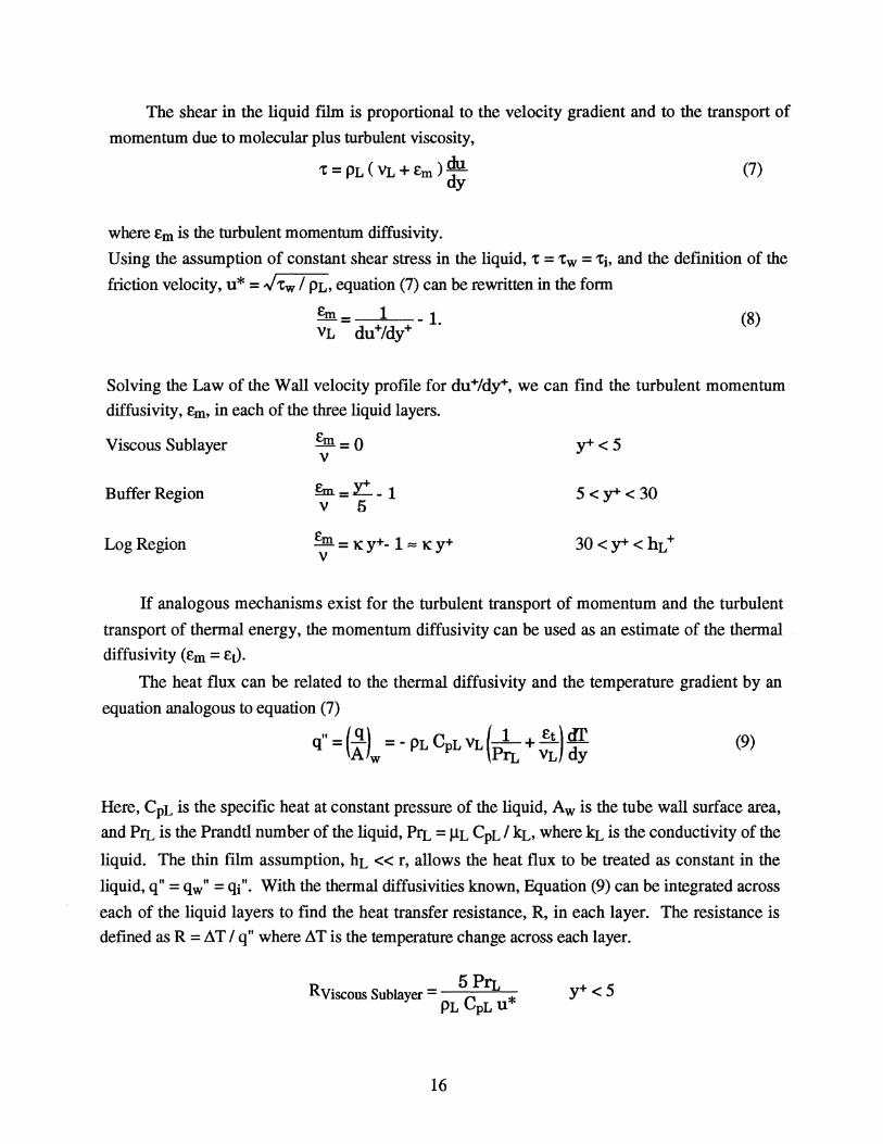
The shear in the liquid ftlm is proportional to the velocity gradient and to the transport of

momentum due to molecular plus turbulent viscosity,

't=PL(VL+£m)~ (7)

where £m is the turbulent momentum diffusivity.

Using the assumption of constant shear stress in the liquid, 't = 'tw = 'tio and the dermition of the

friction velocity, u* = -J'tw / PL, equation (7) can be rewritten in the form

(8)

Solving the Law of the Wall velocity proftle for du+/dy+, we can find the turbulent momentum

diffusivity, em, in each of the three liquid layers.

Viscous Sublayer £m=o y+<5 v

Buffer Region fuL=r_l 5<y+<30 v 5

Log Region £ 30<y+<hL+ -In. = lCy+- 1 = lCy+ V

If analogous mechanisms exist for the turbulent transport of momentum and the turbulent

transport of thermal energy, the momentum diffusivity can be used as an estimate of the thermal

diffusivity (£m = BU. The heat flux can be related to the thermal diffusivity and the temperature gradient by an

equation analogous to equation (7)

" ( q) C (1 £t) err q=- =-PL pLVL-+---A w PIL VL dy

(9)

Here, CpL is the specific heat at constant pressure of the liquid, Aw is the tube wall surface area,

and PlL is the Prandd number of the liquid, PlL = ilL CpL / kL, where kL is the conductivity of the

liquid. The thin ftlm assumption, hL « r, allows the heat flux to be treated as constant in the

liquid, q" = qw" = qi". With the thermal diffusivities known, Equation (9) can be integrated across

each of the liquid layers to find the heat transfer resistance, R, in each layer. The resistance is

defined as R = AT I q" where AT is the temperature change across each layer.

5PIL R Viscous Sublayer = C *

PL pLU

16

R . _ 5 In (l + 5 PrL) Buffer Regton - p C u *

L pL

RLo n . _ ~ln(!Jt) g n.eglOn - C *

PL pL U

where u* = -Iii 'V PI.

The liquid resistance network can be used to estimate a heat transfer coefficient based on the

average inner wall temperature, Tw,in, and the liquid-vapor interface temperature, Ti.

" HTC= q Twin - Ti ,

Using the resistance network we find

HTC = PL CpL u*

5PrL+5In(1+5 PrL) + LIn (hL+) K 30.

(10)

where u* = -Iii 'V PI.

The accuracy of this estimate depends on the following assumptions:

1) The tube wall resistance is negligible, i.e. Tw,out = Tw,in.

2) The heat transfer resistance in the vapor is small compared to the resistance in the

liquid. This is true if most of the energy transfer at the interface goes into phase change

resulting in a very small temperature gradient in the vapor phase.

3) The liquid interface temperature is circumferentially unifonn.

4) The tube wall temperature is circumferentially unifonn. This is true if the interface

temperature, the external boundary conditions, and the liquid f11m thickness all do not

vary circumferentially.

5) The bulk temperature is approximately equal to the interface temperature.

The bulk temperature is defmed as,

17

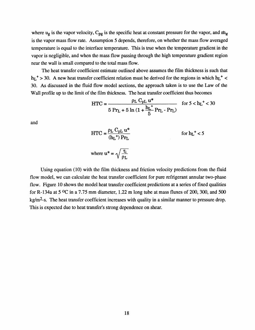
where Ug is the vapor velocity, Cpg is the specific heat at constant pressure for the vapor, and Iilg

is the vapor mass flow rate. Assumption 5 depends, therefore, on whether the mass flow averaged

temperature is equal to the interface temperature. This is true when the temperature gradient in the

vapor is negligible, and when the mass flow passing through the high temperature gradient region

near the wall is small compared to the total mass flow.

The heat transfer coefficient estimate outlined above assumes the film thickness is such that

hL + > 30. A new heat transfer coefficient relation must be derived for the regions in which hL + < 30. As discussed in the fluid flow model sections, the approach taken is to use the Law of the

Wall profile up to the limit of the fIlm thickness. The heat transfer coefficient thus becomes

HTC = PL CpL u* for 5 < hL + < 30

5 P1L + 5ln (1 + hL+ PIL - PIL) 5

and

where u* = -/'ti 'VPJ;

Using equation (10) with the film thickness and friction velocity predictions from the fluid

flow model, we can calculate the heat transfer coefficient for pure refrigerant annular two-phase

flow. Figure 10 shows the model heat transfer coefficient predictions at a series of fixed qualities

for R-134a at 5 0C in a 7.75 mm diameter, 1.22 m long tube at mass fluxes of 200,300, and 500

kglm2-s. The heat transfer coefficient increases with quality in a similar manner to pressure drop.

This is expected due to heat transfer's strong dependence on shear.

18

10000 -0- Wattelet - A -0- Wattelet - B -6- Wattelet - C

8000 ___ Model- A ...... _Model- B ~ _Model- C I

"S 6000 .....

~

U

~ 4000

2000

0 0 0.2 0.4 0.6 0.8 1

Quality

Figure 10 Comparison of evaporation heat transfer coefficients from the uniform film thickness model and Wattelet's (1994) experimental results for R134a (Horizontal D = 7.75 mm L= 1.22m T=50 C)

Table 3 Percentage of thermal resistance in the three liquid film layers for the R134a conditions shown in Figure 10 at a mass flux of 300 kglm2-s.

Quality RVisc% RBuff% RLog%

0.2 51.4 39.3 9.3 0.3 51.8 39.6 8.6 0.4 52.3 40.0 7.8 0.5 52.8 40.4 6.8 0.6 53.5 40.9 5.7 0.7 54.3 41.5 4.2 0.8 55.5 42.4 2.2 0.9 58.3 41.7 0.0

Table 3 shows the importance of the viscous sub layer and buffer regions as thermal resistance

layers. Although significantly thinner than the log region over most of the qUality range, the

viscous sub layer and buffer region account for over 90 percent of the thermal resistance. This

observation is important from a modeling perspective. If the log region can be assumed well

19

mixed, a more detailed description of the complex flow field in this region may not be necessary

for accuracy in heat transfer predictions. Rohsenow, et al. (1956), expressed a similar thought in

response to a comment by Seban: "Realizing that the region of expected error is also a region of

very small resistance to heat flow when compared to the 'buffer' layer and the laminar sublayer, it

is felt that deviations in this area will have but little effect on the predicted values of heat-transfer

coefficient for the entire film."

The current model assumes no differences between evaporation and condensation processes.

The effects of evaporation and condensation on the transfer of momentum between the phases is

not considered, however, as shown by Wattelet (1994), the momentum exchange due to phase

change is generally a small effect for refrigerants. Applying the model to both evaporation and

condensation results indicates some of the differences between these two processes.

Figure 10 shows significant deviation between the model and Wattelet's (1994) data at high

mass flux. The relatively thin liquid film may tend to dry out on the upper tube surface, thus

reducing the heat transfer coefficient.

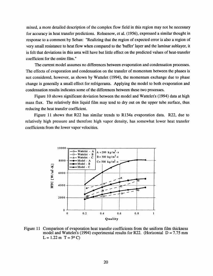
Figure 11 shows that R22 has similar trends to R134a evaporation data. R22, due to

relatively high pressure and therefore high vapor density, has somewhat lower heat transfer

coefficients from the lower vapor velocities.

......

10000u===========,-----------------,------r A =200 kg/m1.s

8000

6000

4000

2000

-0- Wattelet - A

B = 300 kg/m2.s -0- Wattelet - B -11- Wattelet - C

c= 500 kg/of.s ........... . -+-Model- A ___ Model- B _Model- C

u .......................... ,i. •••••••••• n ••••••••• .......................... ?_ ........................ -:-......... · ...... H ............. .

I ! iy-

.... · .. · .... ···· .. · .... ·· .. ····r········:;::··--··:=:r···· i­! :

.1 ! - L' ____ ~r-

O~----~~----~------~------~----~ o 0.2 0.4 0.6 0.8

Quality

Figure 11 Comparison of evaporation heat transfer coefficients from the uniform film thickness model and Wattelet's (1994) experimental results for R22. (Horizontal D = 7.75 mm L = 1.22 m T = 50 C)

20

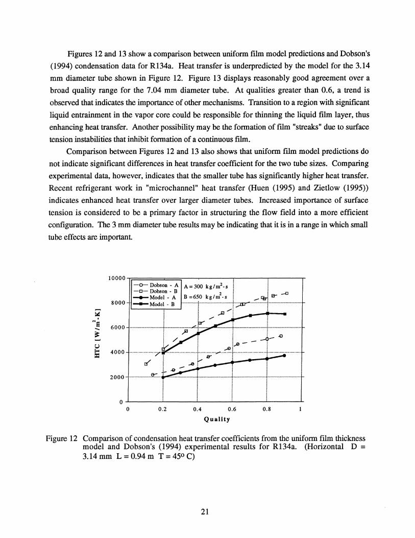
Figures 12 and 13 show a comparison between uniform film model predictions and Dobson's

(1994) condensation data for R134a. Heat transfer is underpredicted by the model for the 3.14

mm diameter tube shown in Figure 12. Figure 13 displays reasonably good agreement over a

broad quality range for the 7.04 mm diameter tube. At qualities greater than 0.6, a trend is

observed that indicates the importance of other mechanisms. Transition to a region with significant

liquid entrainment in the vapor core could be responsible for thinning the liquid film layer, thus

enhancing heat transfer. Another possibility may be the formation of fIlm "streaks" due to surface

tension instabilities that inhibit formation of a continuous fIlm.

Comparison between Figures 12 and 13 also shows that uniform [llm model predictions do

not indicate significant differences in heat transfer coefficient for the two tube sizes. Comparing

experimental data, however, indicates that the smaller tube has significantly higher heat transfer.

Recent refrigerant work in "microchannel" heat transfer (Huen (1995) and Zietlow (1995))

indicates enhanced heat transfer over larger diameter tubes. Increased importance of surface

tension is considered to be a primary factor in structuring the flow field into a more efficient

configuration. The 3 mm diameter tube results may be indicating that it is in a range in which small

tube effects are important

10000

8000 ....... ~ . .os

6000 .... ~ .... u S 4000

2000

-0- Dobson· A A= 300 kg/m2-s -0- Dobson - B 2 ' -c ___ Model - A B =650 kg/m -s. _ cei e----Model - B ··········l·············~··::::r;;m-···········l··········· ............ .

. b-- : ........................... l. ................... u •• ~ .. ~.uu.. : : I / ~: .. · ...... l .................. ·J·= .. ~ ............ ..

. L,.e-- i .. · .... ·· ........ ··7 ~· .. ·· .. ········ ...... ·f·· .... ,e;m_··~·t····m ........ m.m .. +m.m::e ... m.m.

../ i i--- :.. [3' i _..e, I,! --mOCM--tommmj----

~ i ~ ! o~------~----~------~------~------~

o 0.2 0.4 0.6 0.8

Quality

Figure 12 Comparison of condensation heat transfer coefficients from the uniform film thickness model and Dobson's (1994) experimental results for R134a. (Horizontal D = 3.14mm L=0.94m T=450C)

21

10000

8000 ....... ~ .

"'e 6000 -~ U E-- 4000

==

2000

0

-0- Dobson - A -0- Dobson - B -+-Model - A

........... Model- B

. . 2 i

A =300 kg/m -s i 2 ; ,...B .e

B = 6.50 kg/m -s i ja ···········T··· .... ···· .... ·········y-············ .... :;;;···T·· ..................... .

I..-___ ---'! I /J"" i

. . . . · . . . ......................... _..................................... . ...... ---_ ........................................ -.......... . · . . . · . . . i : :;..' ! ! ; :.-!'"o 1 1

......................... 1. ;/·········~·····I·························t···;···:;;···~ ... t-... ::? ............. . ~ 1 ~~~~~~~-t--~ 13" 1 -&->0-:

1 e- - . . =r---r-r o 0.2 0.4 0.6 0.8

Quality

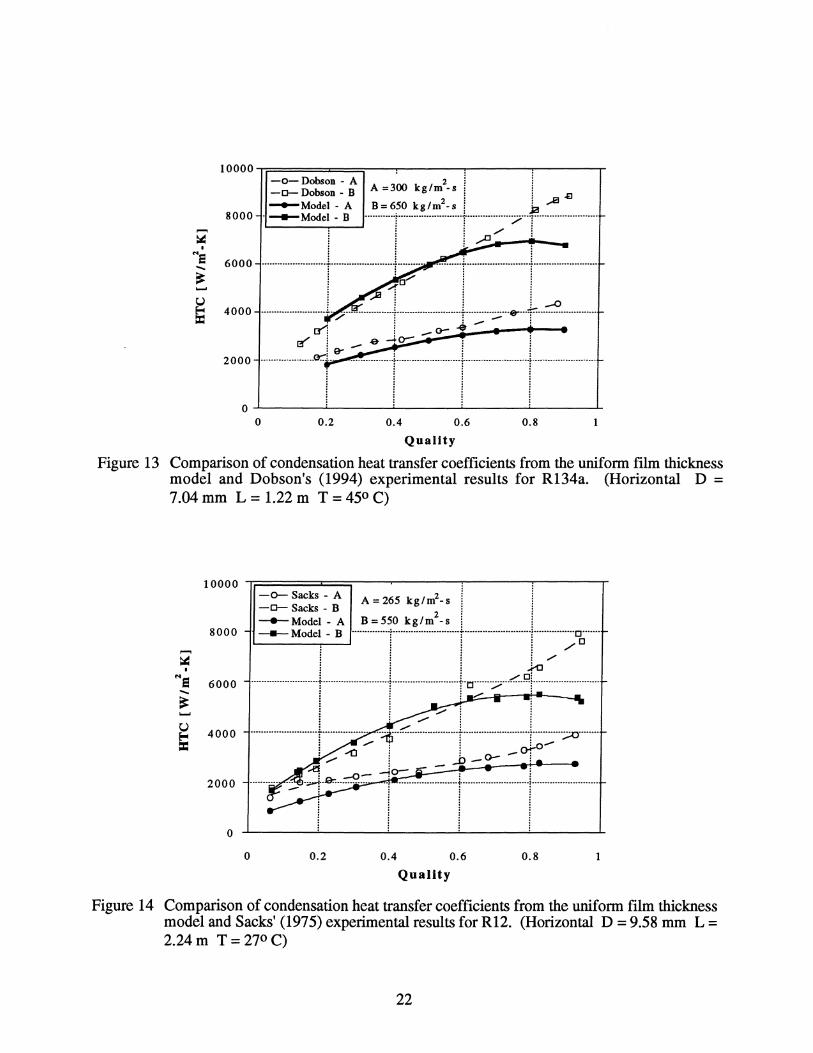
Figure 13 Comparison of condensation heat transfer coefficients from the uniform film thickness model and Dobson's (1994) experimental results for R134a. (Horizontal D = 7.04 mm L = l.22 m T = 450 C)

10000 ~~~~~~,--~----r----~----r -0- Sacks - A A = 265 kg/m2-s -0- Sacks - 8 2 ---Model - A 8=550 kg/m-s ----- Model - 8 ........ ·······[····· ...... · .............. t ...... ················ .. ··f .............. ··0 ...... ·

iii /0 8000

1 1 1 /'

6000 .................... · .. · .. t .......................... I· .... ···· .... ··· ...... ·· .. j .. o ....... / ... <'!':':.~ ..................... . : : . : ! ~ i ; .'/ . . · .. ······ .... · ............ r .... ····· .. ····~ ··1i· ................ ··· .... ·r······· .... ··· ...... · .. ·T~·::: .. ·':;O ...... ··

: ..-0: : _ot" '/ 1 -0-0-; ~ : - .

4000

2000 .......... . . ~.~~ '"=1--1----o

o 0.2 0.4 0.6 0.8

Quality

Figure 14 Comparison of condensation heat transfer coefficients from the uniform film thickness model and Sacks' (1975) experimental results for R12. (Horizontal D = 9.58 mm L = 2.24 m T = 270 C)

22

Figure 14 compares R12 condensation data in a 9.58 mm diameter tube (Sacks (1975)) to the

uniform film modeL Heat transfer coefficients show similar agreement as seen in the 7 mm tube

for R134a in Figure 13. A deviation between the uniform film model and experimental trends

occurs for R12 in the 9 mm tube, however, the deviation occurs at a higher quality level than that

observed for R134a in the 7 mm tube.

Figure 15 shows a comparison between the film model and Rll data from Sacks (1975) in

the 9.58 mm diameter tube. The data is modeled reasonably well over the range of available data.

Similar to the pressure drop trends, Rll, with relatively high vapor velocities, may tend to be in a

range with a reasonably uniform film.

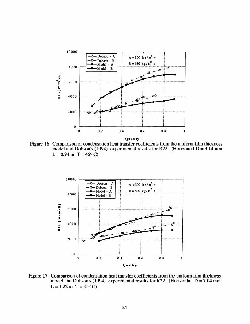
Figure 16, 17, and 18 show comparisons between R22 model predictions and data from

Sacks and Dobson. This is the only data set between the two studies with a common refrigerant.

The uniform film model, in Figure 16, shows a tendency to underpredict Dobson's smaller tube

heat transfer. This is similar to the trend seen for the small tube results for R134a. Similar trends

are observed for Dobson's and Sacks' data in Figures 17 and 18 for tubes that are similar in size.

6000 2 ;

o Sacks - 260 kg/m - s i

5000

,...., ~ • 4000 fOe -~

3000

• Mod.] - 260 k"m'-'It--························r············~·······~····~··········~······r·······················r··············· ...... .

·························+············· ... ········1··························1·························+······ .................. . U E--

= 2000

i!!l iii ·······················t·························I··························I·························t····· .................... ~

1000 .... ~ ................. !. ....................... ./. ........................ ./. ....................... .1 ........................ . ! ! ! !

0 iii i

0 0.2 0.4 0.6 0.8

Quality

Figure 15 Comparison of condensation heat transfer coefficients from the uniform film thickness model and Sacks' (1975) experimental results for Rl1. (Horizontal D = 9.58 mm L = 2.24 m T = 300 C)

23

10000

8000

t? Ole 6000 -~ U Eo! 4000 =

-a-Dobson - A A=300 kg/m2-s 1 -[]- Dobson - B 2: --.- Model - A B = 650 kg/m - s i -.-Model - B ... --i ................ · ........ · ..... , ... · ••• · ••• · .......... • .... ···+···0·················

! ! .Ml--ar . ! ..... 01" : :.JiiI ...................... ·t ...... · .................. !·· .. ··· .. ..

....................... 1

2000

0 0 0.2 0.4 0.6 0.8 1

Quality

Figure 16 Comparison of condensation heat transfer coefficients from the uniform film thickness model and Dobson's (1994) experimental results for R22. (Horizontal D = 3.14 mm L = 0.94 m T = 450 C)

10000 -0- Dobson - A -CJ- Dobson - B ---Model - A

8000 ...... ----Model - B

~ 6000 Ole -~ U 4000 Eo!

= 2000 CY

0 0 0.2 0.4

A =300 kg/m2_s 2

B = 500 kg/m -s

0.6

Quality

0.8

Figure 17 Comparison of condensation heat transfer coefficients from the uniform ftlm thickness model and Dobson's (1994) experimental results for R22. (Horizontal D = 7.04 mm L = 1.22 m T = 450 C)

24

10000

----Model - B 8000

~ . 1:

6000 ..... ~ U Eo<

= 4000

--e-Sacks - A A=240 kg/rn2-s ~Sacks - B -'-Model _ A B =490 kg/rn2_s

_ .... _. __ ..... ; ........ __ ........... _____ ). __ .... _._0 .. _- __ o_ •••••• v •.. _ ......... .

, I ! do 0 •

................................................... 1 •••••••••.•••••••.•••••••. l •••...•.. ~~~.!'!' ••.. ~ ••• hI. r.:: ... :'=i .• r-... :::": .. ! ! :

I! ;°,,0;

~==~--r~

[J

2000 --1----TI 0

0 0.2 0.4 0.6 0.8

Quality

Figure 18 Comparison of condensation heat transfer coefficients from the uniform film thickness model and Sacks' (1975) experimental results for R22. (Horizontal D = 9.58 mm L = 2.24 m T = 270 C)

Conclusions

The uniform film model developed in this work provides a basis for understanding some of

the mechanisms and trends involved in two-phase flow and heat transfer of refrigerants. Three

types of refrigerants (high, mid-range, and low pressure) have been compared to the model.

Generally, the low pressure refrigerant (Rll) compares reasonably well in terms of pressure drop

and heat transfer. Although the vapor density and transport properties are significantly different

from the air-water system used for development of an interfacial shear stress model, other

refrigerants in the low pressure range may also have reasonable agreement to a uniform fIlm model

over a relatively wide range of mass fluxes and qualities.

Mid-range and higher pressure refrigerants (R134a, R12, R22), which have higher vapor

densities, show systematic deviations in pressure drop predictions from the uniform film model.

Peak pressure drop at high qualities appears to indicate a flow structure that has other significant

loss mechanisms than those modeled by a uniform film. Heat transfer is predicted reasonably well

for evaporation at low mass fluxes, but the model over-predicts heat transfer at high mass fluxes.

The over-prediction may be caused by a non-uniform film in which a thinner, upper tube region is

prone to dryout. Condensation heat transfer data compares reasonably well with predictions over a

broad quality and mass flux range, however, two areas of deviation from model predictions are

25

observed. First, heat transfer predictions are consistently low for results from a 3 mm diameter

tube indicating that geometry may be significant as diameters reduce below that size. Second, high

quality regions show increased heat transfer over the uniform model predictions, indicating other

mechanisms are dominating the flow field and resulting heat transfer effects.

Acknowledgements

The authors are grateful for support from the Air Conditioning and Refrigeration Center

Project #45, an NSF sponsored, industry research center located at the University of Illinois at

Urbana-Champaign.

References

Asali, J. c., Hanratty, T. J., Andreussi, P. 1985 Interfacial drag and film height for vertical annular flow. AIChE J. 31, 895-902.

Carey, V. P. 1992, Liquid-Vapor Phase Change Phenomena, Hemisphere, New York, pp. 409-410.

Carpenter, E. F. and A. P. Colburn 1951 The effect of vapor velocity on condensation inside tubes, Proceedings of the General Discussion of Heat Transfer, The Institution of Mechanical Engineers and The American Society of Mechanical Engineers, 20-26.

Davies, J. T. 1972 Turbulence Phenomena, An Introduction to the Eddy Transfer of Momentum, Mass, and Heat, Particularly at Interfaces, Academic Press, Ch. 4.

Dobson, M. K. 1994 Heat Transfer and Flow Regimes During Condensation in Horizontal Tubes, Ph.D. Thesis, University of Illinois, Urbana-Champaign.

DOE 1993 Energy Efficient Alternatives to Chlorofluorocarbons (CFCs), U.S. Dept. of Energy, Report No. DOFlERl30115-Hl.

Gallagher, J., M. McLinden, G. Morrison, and M. Huber, 1993, NIST thermodynamic properties of refrigerant and refrigerant mixtures, version 4.01, National Institute of Standards and Technology, Gaithersburg, MD.

Henstock, W. H., Hanratty, T. J. 1976 The interfacial drag and the height of the wall layer in annular flows. AIChE J. 22, 990-1000.

Huen, M. K. 1995 Performance and optimization of microchannel condensers, Ph.D. Thesis, University of Illinois, Urbana-Champaign.

Incropera, F. P. and D. P. DeWitt, 1985, Fundamentals of heat and mass transfer, John Wiley and Sons, NY, NY.

Jung, D. S. and Radermacher, R. 1991 Prediction of heat transfer coefficients of various refrigerants during evaporation, ASHRAE Transactions, 97, Pt. 2.

Kandlikar, S. G. 1990 A general correlation for saturated two-phase boiling heat transfer inside horizontal and vertical tubes, Journal of Heat Transfer, 112, pp. 219-228.

Karman, T. V. 1939 The analogy between fluid friction and heat transfer, Transaction of the A.S.M.E., 61, 705-710.

Newell, T. A. 1996 A report on global warming and energy consumption trends of major appliances. contract report to the Association of Home Appliance Manufacturers (AHAM).

26

Pierre, B. 1956 The coefficient of heat transfer for boiling freon-12 in horizontal tubes, Heating and Air Treatment Engineer, pp. 302-310.

Rohsenow, W. M., Webber, J. H., and Ling, A. T. 1956 Effect of Vapor Velocity on Laminar and Turbulent-Film Condensation, Transactions of the A.S.M.E., pp. 1637-1643.

Sacks, P. S. 1975 Measured characteristics of adiabatic and condensing single-component two­phase flow of refrigerant in a 0.377 inch diameter horizontal tube, ASME paper 75-W NHT-24.

Shah, M. M. 1976 A new correlation for heat transfer during boiling flow through pipes, ASHRAE Transactions, 82, Part 2, pp. 66-86.

Smith, M. K. 1993, Analysis of dual-load vapor compression cycle using non-azeotropic refrigerant mixtures, Ph.D. Thesis, Univerisity of Dlinois, Urbana-Champaign.

Souza, A. L., Pimenta, M. M. 1995 Prediction of pressure drop during horizontal two-phase flow of pure and mixed refrigerants, ASMFJJSME Summer Meeting, Aug. 13-18, 1995.

Wattelet, J. P. 1994 Heat Transfer Flow Regimes of Refrigerants in a Horizontal-Tube Evaporator, Ph.D. Thesis, University of illinois, Urbana-Champaign.

Whalley, P. B. 1987 Boiling, Condensation, and Gas-Liquid Flow. Clarendon Press, Oxford, P. 12. Zietlow, D. 1995, Heat transfer and flow characteristics of condensing refrigerants in" small­channel crossflow heat exchangers, Ph.D. Thesis, University of Dlinois, Urbana-Champaign.

27