CHARACTERIZATION AND ESTIMATION OF

POWER GENERATION POTENTIALS OF SOME

AGRICULTURAL WASTES

A THESIS SUBMITTED IN PARTIAL FULFILLMENT OF THE REQUIREMENTS

FOR THE DEGREE OF

Master of Technology(Research)

in

Mechanical Engineering

by

SATYABRATA TRIPATHY Roll No: 612ME103

Dept. of Mechanical Engineering

National Institute of Technology, Rourkela 2015

CHARACTERIZATION AND ESTIMATION OF

POWER GENERATION POTENTIALS OF SOME

AGRICULTURAL WASTES

A THESIS SUBMITTED IN PARTIAL FULFILLMENT OF THE REQUIREMENTS

FOR THE DEGREE OF

Master of Technology(Research)

in

Mechanical Engineering

by

SATYABRATA TRIPATHY Roll No: 612ME103

Under the supervision of

Prof. S. K. Patel and Prof. M. Kumar

Dept. of Mechanical Engineering

National Institute of Technology, Rourkela 2015

i | P a g e

Declaration

I hereby declare that the work which is being presented in this thesis entitled

“Characterization and Estimation of Power Generation Potentials of Some Agricultural

Wastes” in partial fulfilment of the requirements for the award of M. Tech. (Research) degree,

submitted to the Department of Mechanical Engineering, National Institute of Technology,

Rourkela, is an authentic record of my own work under the supervision of Prof. S. K. Patel and

Prof. M. Kumar. I have not submitted the matter embodied in this thesis for the award of any

other degree to any other university or institute.

Place:

Date: SATYABRATA TRIPATHY

ii | P a g e

NATIONAL INSTITUTE OF TECHNOLOGY ROURKELA

Certificate

This is to certify that the thesis entitled “Characterization and Estimation of Power

Generation Potentials of Some Agricultural Wastes” submitted by Satyabrata Tripathy,

Roll no. 612ME103 has been carried out under my supervision in partial fulfilment of the

requirements for the award of Master of Technology (Research) degree in Mechanical

Engineering with specialization in Thermal Engineering at National Institute of Technology,

Rourkela, and this work has not been submitted to any other University/Institute for the award of

any degree.

Prof. S. K. Patel Prof. M. Kumar

Principal Supervisor Co-supervisor

Department of Mechanical Engineering Department of Metallurgy and Materials

Engineering

National Institute of Technology, Rourkela National Institute of Technology, Rourkela

Email: skpatel@nitrkl.ac.in Email: mkumar@nitrkl.ac.in

iii | P a g e

ACKNOWLEDGEMENT

I express my deep sense of gratitude and indebtedness to my supervisors Prof. S.K. Patel

and Prof. M. Kumar for providing precious guidance, constant encouragement and inspiring

advice throughout the course of this work and for propelling me further in every aspect of my

academic life. Their presence and optimism has provided an invaluable influence on my career

and outlook for the future. I consider it my good fortune to have an opportunity to work with two

such wonderful persons.

I am grateful to Prof. S. S. Mahapatra, Head of the Department of Mechanical

Engineering for providing me the necessary facilities for smooth conduct of this work. I am also

grateful to Mr. Bhanja Nayak, Fuel Laboratory, Metallurgical and Materials Engineering for his

assistance in experimental work. I am also thankful to all the staff members of the department of

Mechanical Engineering and department of Metallurgical and Materials Engineering and to all

my well-wishers for their inspiration and assistance. I would also like to thank Dilip Kumar

Bagal, M.Tech. (Research) student of Mechanical Engineering department for helping in

software work.

Satyabrata Tripathy

Roll no. 612ME103

Mechanical Engineering

National Institute of Technology, Rourkela

iv | P a g e

Abstract

India is developing at an incredible rate. With development, there is an alarming increase in

the demand for energy. But at the same time, we as a nation, have to economize on our energy

costs to focus on human developmental needs. It is an undeniable fact that we have to strive for

energy self-sufficiency to stay relevant in the modern times we live in. In such context, the idea

of biomass energy becomes very important and relevant. With its inherent advantages of carbon

neutrality and sustainability, biomass energy is the way forward for the nation and the world at

large. Biomass energy has the potential and the promise of becoming the prime energy source.

Though many forms of bioenergy are in focus of many research and development

agencies/organizations, harnessing the biomass energy through combustion is the simplest

method. In this project, we attempt to analyse and discuss the feasibility and sustainability of this

method. We would have to dwell upon the challenges posed by this method and attempt to quell

these in a scientific manner. Abundant land and water resources are the major enabler for

adoption of biomass energy, as a principle. But in practice, technical variables such as calorific

value, ash content, presence of sulphur, greenhouse gas emissions play a significant role in the

actual adoption of biomass as a major source of energy. To study these, we have chosen wastes

of six different agriculture based biomass species such as banana (Musa acuminate), coconut

(Cocos nucifera), arecanut (Areca catechu), rice (Oryza sativa), wheat (Triticum aestivum) and

palm (Borassus flabellifer). The samples were analysed by proximate and ultimate analyses, and

further correlation was established through regression analysis. Proximate analysis showed that

the coconut has the highest volatile matter content (i.e., 73 wt.%) and banana has the highest

fixed carbon content (i.e., 20 wt.%) which indicated higher calorific values. The determination of

calorific values validated the former results. Palm exhibited lowest ash content suggesting no ash

related problems during combustion. Ultimate analysis performed on some of the selected

v | P a g e

species showed high carbon and hydrogen contents in the leaves of coconut and arecanut. Out of

some selected biomass ashes tested for their fusion temperatures, rice has the lowest initial

deformation temperature (i.e., 938 0C) which is substantially above the boiling temperature,

suggesting that all the selected biomass samples can be used safely for combustion in boilers up

to a temperature of 800 0C. The bulk density of rice husk has been found out to be the highest

(i.e., 336.257 kg/m3), suggesting facilitation of higher amount of rice husk in the boiler and,

economical transportation and handling. An attempt has been made to develop empirical

formulae statistically using regression analysis to predict gross calorific value using proximate

and ultimate analyses data. The land requirements for energy plantation with selected biomass

species were computed and found that approximately 4931, 524, 1757, 814, 3043 and 1146

hectares of land for harvesting banana, coconut, arecanut, palm, wheat and rice biomass species

for assuring a perpetual supply of electricity at the rate of 5475 MWh per year for a group of 10-

12 villages consisting of about 2000 households. Further, from the calculations of fuel

requirement it was observed that coal requirement can decrease from 4968.0 to 4289.1 t/year and

4968 to 4008.6 t/year with the increase in biomass content from 0 to 15 % in the briquettes of

coal with rice husk and coal with palm leaf respectively which suggests that agricultural biomass

wastes can be used in co-firing mode for generation of electricity by substituting a portion of

coal.

Key words: Ash fusion temperature, Biomass, Bulk density, Calorific value, Proximate analysis,

Regression analysis, Ultimate analysis

vi | P a g e

NOMENCLATURE

∆T Maximum rise in temperature

∑(Y − Y)2 Variation of Y value around regression line

∑(Y − Y)2 Variation of Y value around own mean

𝑎0, 𝑎1 Constant parameters

AAE Average absolute error

ABE Average bias error

AC Ash content

AFTs Ash fusion temperatures

CHP Combined heat and power plant

CSP Concentrated solar thermal power plant

FC Fixed carbon content

FT Flow temperature

GCV Gross calorific value

GDP Gross domestic product

HHV Higher heating value

HT Hemispherical temperature

IDT Initial deformation temperature

K Number of independent variables

MC Moisture content

MRA Multiple regression analysis

MSW Municipal solid waste

N Number of data points in the sample

R Coefficient of correlation

R2 Coefficient of determination

RET Renewable energy technologies

S Standard error of estimate

SLRA Simple linear regression analysis

SRA Simple regression analysis

ST Softening temperature

VM Volatile matter content

W Initial weight of dried sample

W.E. Water equivalent of apparatus

wt. % Weight percentage

X Independent variable

Y Sample values of dependent variables

Y Corresponding estimated values from regression analysis

vii | P a g e

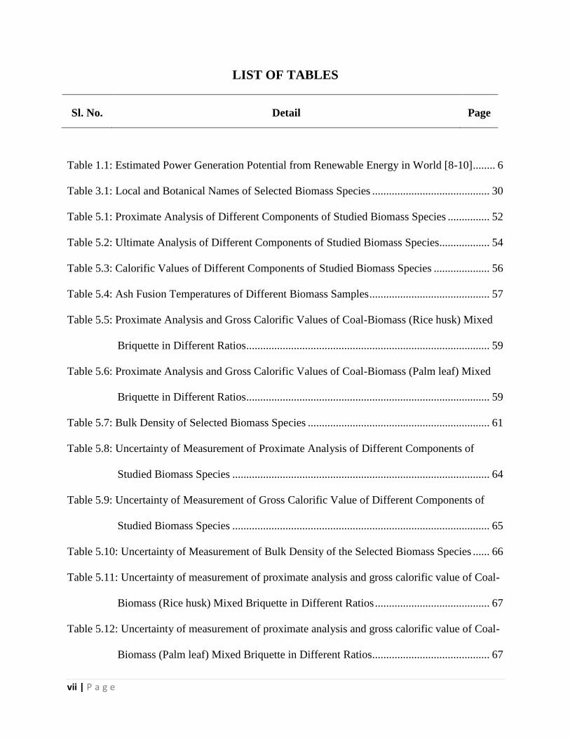
LIST OF TABLES

Sl. No. Detail Page

Table 1.1: Estimated Power Generation Potential from Renewable Energy in World [8-10] ........ 6

Table 3.1: Local and Botanical Names of Selected Biomass Species .......................................... 30

Table 5.1: Proximate Analysis of Different Components of Studied Biomass Species ............... 52

Table 5.2: Ultimate Analysis of Different Components of Studied Biomass Species.................. 54

Table 5.3: Calorific Values of Different Components of Studied Biomass Species .................... 56

Table 5.4: Ash Fusion Temperatures of Different Biomass Samples ........................................... 57

Table 5.5: Proximate Analysis and Gross Calorific Values of Coal-Biomass (Rice husk) Mixed

Briquette in Different Ratios ....................................................................................... 59

Table 5.6: Proximate Analysis and Gross Calorific Values of Coal-Biomass (Palm leaf) Mixed

Briquette in Different Ratios ....................................................................................... 59

Table 5.7: Bulk Density of Selected Biomass Species ................................................................. 61

Table 5.8: Uncertainty of Measurement of Proximate Analysis of Different Components of

Studied Biomass Species ............................................................................................ 64

Table 5.9: Uncertainty of Measurement of Gross Calorific Value of Different Components of

Studied Biomass Species ............................................................................................ 65

Table 5.10: Uncertainty of Measurement of Bulk Density of the Selected Biomass Species ...... 66

Table 5.11: Uncertainty of measurement of proximate analysis and gross calorific value of Coal-

Biomass (Rice husk) Mixed Briquette in Different Ratios ......................................... 67

Table 5.12: Uncertainty of measurement of proximate analysis and gross calorific value of Coal-

Biomass (Palm leaf) Mixed Briquette in Different Ratios.......................................... 67

viii | P a g e

Table 5.13: Developed Regression Equations for the Estimation of the Gross Calorific Values of

Studied Biomass Samples from Proximate Analysis Data and Their Statistical

Performance Measures .............................................................................................. 70

Table 5.14: Developed Regression Equations for the Estimation of the Gross Calorific Values of

Studied Biomass Samples from Ultimate Analysis Data and Their Statistical

Performance Measures .............................................................................................. 73

Table 5.15: Total Energy Contents and Power Generation Structure for Banana ........................ 75

Table 5.16: Total Energy Contents and Power Generation Structure from Coconut Biomass

Species ....................................................................................................................... 76

Table 5.17: Total Energy Contents and Power Generation Structure from Arecanut Biomass

Species ....................................................................................................................... 76

Table 5.18: Total Energy Contents and Power Generation Structure from Rice Biomass Species

....................................................................................................................................................... 77

Table 5.19: Total Energy Contents and Power Generation Structure from Wheat Biomass

Species ....................................................................................................................... 77

Table 5.20: Total Energy Contents and Power Generation Structure from Palm Biomass Species

....................................................................................................................................................... 77

Table 5.21: Land Required for Energy Plantation of Different Agricultural Biomass Species for

generating 15 MWh per day ...................................................................................... 79

Table 5.22: Energy Content from Coal-Rice Husk Blends........................................................... 80

Table 5.23: Energy Content from Coal-Palm Leaf Blends ........................................................... 80

Tables 5.24: Fuel Required for Coal-Rice Husk Briquettes ......................................................... 83

Tables 5.25: Fuel Required for Coal-Palm Leaf Briquettes ......................................................... 83

ix | P a g e

LIST OF FIGURES

Sl. No. Detail Page

Fig 1.1: Estimated Power Generation Potential from Renewable Energy in India ....................... 7

Fig 1.2: Installed Power Generation Potential from Renewable Energy in India .......................... 8

Fig 3.1: Bomb Calorimeter ........................................................................................................... 35

Fig 3.2: Leitz Heating Microscope………………………………………………………….……37

Fig 3.3: Different Ash Fusion Temperatures ................................................................................ 39

x | P a g e

CONTENTS

Sl. No. Detail Page

Declaration i

Certificate ii

Acknowledgement iii

Abstract iv

Nomenclature vi

List of Tables vii

List of Figures ix

Chapter 1 INTRODUCTION .......................................................................................................... 1

1.1 Overview ................................................................................................................................. 2

1.2 Biomass ................................................................................................................................... 4

1.2.1 Applications of biomass energy .................................................................................. 4

1.3 Why Biomass Energy? ............................................................................................................ 5

1.4 Electric Power Generation Potential of Renewables ............................................................... 5

1.5 Biomass Conversion Process................................................................................................... 8

1.5.1 Combustion ................................................................................................................. 8

1.5.2 Thermochemical process ............................................................................................. 9

1.5.3 Biochemical conversion ............................................................................................ 10

1.6 Biomass: Potential Substitute of Coal for Power Generation ............................................... 10

xi | P a g e

1.6.1 Biomass co-firing technology ................................................................................... 11

1.7 Benefits of Utilizing Biomass for Power Generation ............................................................ 12

Chapter 2 LITERATURE REVIEW ............................................................................................. 14

2.1 Introduction ........................................................................................................................... 15

2.2 An Outline of Energy Challenges in India ............................................................................ 15

2.3 Renewable Energy Scenario .................................................................................................. 16

2.4 Biomass and its Potential ...................................................................................................... 18

2.5 Biomass Conversion Process................................................................................................. 20

2.6 Fuel Characteristic of Biomass .............................................................................................. 22

2.7 Ash Fusion Temperature ....................................................................................................... 23

2.8 Co-firing of Biomass with Coal ............................................................................................ 24

2.9 Regression Analysis on the basis of Proximate and Ultimate Analysis ................................ 25

2.10 Decentralized Power Generation ........................................................................................... 26

2.11 Summary ............................................................................................................................... 26

2.12 Objectives .............................................................................................................................. 27

Chapter 3 EXPERIMENTAL WORK .......................................................................................... 28

3.1 Introduction ........................................................................................................................... 29

3.2 Selection of Materials ............................................................................................................ 29

3.3 Proximate Analysis ................................................................................................................ 30

3.3.1 Determination of moisture content ............................................................................ 31

3.3.2 Determination of ash content .................................................................................... 31

xii | P a g e

3.3.3 Determination of volatile matter ............................................................................... 32

3.3.4 Determination of fixed carbon content ...................................................................... 33

3.4 Calorific Value Determination .............................................................................................. 33

3.5 Determination of Ash Fusion Temperatures ......................................................................... 36

3.6 Ultimate Analysis .................................................................................................................. 40

3.7 Bulk Density of the Selected Agricultural Residues ............................................................. 40

3.8 Uncertainty of Measurement ................................................................................................. 40

3.8.1 Standard Deviation .................................................................................................... 41

3.8.2 Propagation of Uncertainty ....................................................................................... 41

Chapter 4 REGRESSION ANALYSIS ........................................................................................ 43

4.1 Introduction ........................................................................................................................... 44

4.2 Regression Analysis .............................................................................................................. 44

4.3 Linear Regression Analysis ................................................................................................... 45

4.3.1 Simple linear regression analysis .............................................................................. 45

4.3.2 Multiple linear regression analysis ............................................................................ 46

4.4 Parameters of Regression Analysis ....................................................................................... 46

4.4.1 Standard error of estimate ......................................................................................... 46

4.4.2 Coefficient of determination ..................................................................................... 47

4.4.3 Coefficient of correlation .......................................................................................... 48

4.5 Evaluation of Errors .............................................................................................................. 48

xiii | P a g e

Chapter 5 RESULTS AND DISCUSSION .................................................................................. 49

5.1 Introduction ........................................................................................................................... 50

5.2 Chemical Compositions of the Studied Biomass Species ..................................................... 50

5.2.1 Proximate analysis ..................................................................................................... 50

5.2.2 Ultimate analysis ....................................................................................................... 53

5.3 Calorific Value ...................................................................................................................... 55

5.4 Ash Fusion Temperatures ...................................................................................................... 56

5.5 Analysis of Co-firing Potentials of Mixed Briquettes of Coal-Selected Biomass Species ... 58

5.6 Bulk Density .......................................................................................................................... 60

5.7 Determination of Uncertainty ................................................................................................ 61

5.8 Regression Analysis .............................................................................................................. 68

5.8.1 Regression analysis performed on proximate analysis data ...................................... 68

5.8.2 Regression analysis performed on ultimate analysis data ......................................... 71

5.9 An Approach for Decentralized Power Generation and Energy Plantation Structure .......... 74

5.9.1 Land requirement for biomass ................................................................................... 75

5.9.2 Fuel Requirement for co-firing with biomass ........................................................... 79

a) Amount of fuel required when proportion of coal-rice husk is 100:0 (i.e., 100 %

coal) 81

b) Amount of fuel required when proportion of coal-rice husk is 90:10 (i.e., 90 % coal

and 10 % rice husk) ................................................................................................................ 81

xiv | P a g e

c) Amount of fuel required when proportion of coal-rice husk is 85:15 (i.e., 85 % coal

and 15 % rice husk) ................................................................................................................ 82

Chapter 6 CONCLUSIONS .......................................................................................................... 85

6.1 Conclusions ........................................................................................................................... 86

6.2 Scope for Future Work .......................................................................................................... 87

REFERENCES ............................................................................................................................. 88

1 | P a g e

2 | P a g e

1. INTRODUCTION

1.1 Overview

Fossil fuels are the primary source of generation of electricity globally. Conventional thermal

power plants and other industries consume enormous quantity of fossil fuel reserves which are

non-renewable and are available in limited quantity. The fast depletion of fossil fuels, economic

issues and environmental concerns over emission from conventional power plants has compelled

researchers to strategize the fuel mix. Therefore, the quest for the alternative sources of

electricity generation which should be eco-friendly and renewable is crucial in order to decrease

our reliance on conventional sources of energy.

In India, about 63 million hectares is covered by forest with a deforestation rate of around 3

lakh ha/year [1]. In addition to the barren land (around 30 million hectares) available for

forestation and forest residues, about 500 MT of agricultural residues are generated every year

from agricultural lands [2]. Agriculture is the mainstay of rural India, constituting 70 % of total

population and 198.9 million hectares of gross cropped area with a cropping intensity of 140.5

%. It also contributes significantly in India’s economic sector with a share of approximately 13.9

% of India’s gross domestic product [3]. Due to wide spread practices of agriculture, lots of

agricultural wastes are generated which remains unutilized.

India stands ninth as the largest economy in world, with GDP growth of 8.7 % and 7.5 % in

the last 5 and 10 years respectively. This eminent rise in economic development is laying

tremendous demand on energy resources which may cause India to confront energy supply

constraints. Around 70 % of electricity generated in India is produced from coal fired plants and

during 2011-12, India was the fourth largest in consumption of natural gas and crude oil [4]. The

3 | P a g e

limited coal resource and other traditional sources make it imperative to explore for an optimal

energy mix in order to manage the imbalance in demand and supply of energy. Exploring and

exploiting alternative source of energy can be the answer to all the questions raised regarding

energy security.

Biomass has become indispensable and enthralling way of power generation in India due its

accessibility, lower investments and high energy potentials. Sustainable production and proper

utilization of biomass can solve the problems in context to energy crisis, climatic concerns,

power transmission losses, waste land development and rural unemployment [5]. Alongside

supplying electricity to national power grids, biomass can be exploited for the opportunities it

offers for decentralized power generation in rural areas. Considering all accounts, exploring and

exploiting biomass can be the most prosperous source of renewable energy for developing

countries including India.

All the projects on biomass have exhibited success hugely, yet the research and total

exploitation of biomass is incipient. The design and efficiency of power plants largely depends

on the properties of bio-fuels which vary from species to species. In order to recognize true

potential of bioenergy in generation of electricity, it is essential to have complete knowledge of

their fundamental properties like energy values, chemical composition including proximate and

ultimate analyses, bulk density, ash fusion temperatures, etc. [6]. Studies and the findings of

proximate analysis, ultimate analysis, calorific values, bulk densities, ash fusion temperatures

and regression analysis to calculate heating values from proximate and ultimate analyses data of

different components of six biomass species namely banana, coconut, arecanut, rice, wheat, and

palm, and their impact on power generation has been outlined and discussed in this project.

4 | P a g e

1.2 Biomass

It is the biodegradable organic material derived from plants, microorganisms, and animals

which includes by-products and residues from agricultural industries, forestry and biodegradable

organic waste from industrial and municipal operation. Biomass is the most promising renewable

energy because of its diverse quality of being used in any state of matter which makes it as the

second largest renewable energy source on earth. World’s total energy consumption is around 12

% which is expected to increase in future [7].

Biomass has become the most valuable renewable energy source of the century due to its

ease of utilization in generation power. Excluding thermochemical and biochemical conversion

processes which are frequently used, the direct combustion of biomass and co-firing it with coal

has increased lot of opportunities and potential of biomass as a source of power generation

because of immense availability, potential to be reused, and absence of pollutants.

1.2.1 Applications of biomass energy

Given the diverse quality of biomass, biomass energy can be applied to various applications

such as:

a) It can be used as solid fuel for combustion to produce heat or it can be also used in combined

heat and power (CHP) plants.

b) It can be blended with fossil fuels (co-firing) to improve efficiency and reduce the residues of

combustion in the boiler.

c) It can potentially replace petroleum as a source of fuel for transportation.

d) In conjunction with fossil fuels biomass can be utilized to generate electricity.

5 | P a g e

1.3 Why Biomass Energy?

Biomass energy is an attractive energy source due to various reasons such as:

a) It is a renewable energy source derived by natural processes as well as a byproduct of human

activity and a surety of long term supplies.

b) It is distributed more evenly all over the world than fossil fuels and can be harnessed by

using more cost effective ways.

c) It provides an opportunity to be more energy self-sufficient and helps in reducing climate

change.

d) Decentralized power generation from biomass offers rural job opportunities. It helps farmers,

ranchers and foresters in managing the waste material in a proper way in order to harness

energy.

1.4 Electric Power Generation Potential of Renewables

According to the Global Status Reports, an estimated 19 % of total energy consumption was

provided by renewable energy sources, with a projection of nearly 25 % by 2040. This demand

of energy was accomplished by modern renewables by an estimation of 4.2 %, hydropower by

3.8 % and 2 % of total energy consumption was provided by wind, solar, geothermal and

biomass in 2014 [8-10].

In 2014, global electric power capacity from renewable energy sources reached a staggering

1560 GW, growth of 8 % over 2012. Apparently from Table 1.1, power generation from biomass

went past 88 GW, growth of 18 % over 2012 and other renewables collectively produced more

than 560 GW which is a growth of 7 % over previous year. Renewable sources contributed more

than 56 % of net additions to electricity generation capacity globally in 2013 [10].

6 | P a g e

Table 1.1: Estimated Power Generation Potential from Renewable Energy in World [8-10]

Technology Electric Power Capacity in GW

2012 2013 2014

Bio-Power 72.0 83.0 88.0

Geothermal Power 11.2 11.7 12.0

Hydropower 970.0 990.0 1000.0

Ocean Power 0.5 0.5 0.5

Solar Power 70.0 100.0 139.0

Concentrated Solar Thermal Power Plant (CSP) 1.8 2.5 3.4

Wind Power 238.0 283.0 318.0

Total 1363.5 1470.7 1560.9

The power generation potential from renewable energy source is estimated to be around

94125 MW as per the report of Ministry of Statistics and Programme Implementation in 2014,

which included power generation from wind (49130 MW), small hydropower (19750 MW),

biomass (17538 MW) and cogeneration bagasse (5000 MW) as shown in Fig. 1.1. The

geographic distribution of estimated power generation capacity from renewables demonstrates

that Karnataka has the highest contribution of about 15.37 % (14464 MW), closely followed by

Gujrat with 13.27 % (12494 MW) and Maharashtra with 10.26 % (9657 MW) [4].

7 | P a g e

Fig 1.1: Estimated Power Generation Potential from Renewable Energy in India [4]

As per the global stipulation on the carbon emission and sustainability through various

changes, Indian energy sector is flourishing and dedicated towards increasing the contribution of

renewable power in total energy production. It has been projected that 15 % of total power

generation will be supplied by renewable energy source by 2020. New initiatives are being

launched by Government of India to restrict the issues related to climate emerging during power

generation. Ministry of New and Renewable Energy together with Ministry of Power has

launched an eco-friendly energy solution initiative called Jawarharlal Nehru National Solar

Mission, with an objective to set up 20000 MW grid of solar power by 2022. In 2012, over 2800

MW capacity of wind energy was installed taking the renewable power capacity up to 22000

MW. In 2011, power generated from solar crossed 100 MW milestone and over 1000 villages of

remote areas were electrified [11]. The installed capacity of power generation from renewable

energy sources are listed in Fig. 1.2.

49130

19750 17538

5000 2707

94125

0

10000

20000

30000

40000

50000

60000

70000

80000

90000

100000

Wind Power SmallHydropower

Biomass Power CogenerationBagasse

Waste toEnergy

Total

Po

wer

Gen

erat

ed i

n M

WEstimated Power Generation Potential from Renewable

Energy in India

8 | P a g e

Fig 1.2: Installed Power Generation Potential from Renewable Energy in India [4]

1.5 Biomass Conversion Process

The progress of biomass conversion technologies has shown tremendous development in

the recent past. Various conversion technologies for generation of electricity from biomass are as

follows.

1.5.1 Combustion

a) Direct Combustion

This is the most common combustion method of feedstock residues like woodchips, sawdust,

bark, bagasse, straw, MSW, etc. This method is employed to produce heat or steam in the boiler

usually in the two stages, first stage is for drying and partial gasification and finally complete

combustion in second stage. This method is not desirable because of generation of high amount

of moisture during combustion [12].

21996.78

3856.68 3135.33 2689.35106.58

2765.81

34550.53

0

5000

10000

15000

20000

25000

30000

35000

40000

Wind SmallHydropower

BiomassPower

BagasseCogeneration

Waste toEnergy

Solar Power Total

Pow

er G

ener

ated

in M

W

Axis Title

Installed Power Generation Potential from Renewable

Energy in India

9 | P a g e

b) Co-firing

Co-firing is a fuel-switching strategy in which two different fuels are used for combustion in

the boiler. In conventional power plants, biomass can be blended with coal in the boiler with

some minor changes. The results from the experiment manifested that around 5-20 % of biomass

can be blended with coal for combustion in boilers. Utilization of biomass along with coal for

power generation has shown huge reduction in emission of carbon dioxide, SOx and NOx [13].

1.5.2 Thermochemical process

a) Pyrolysis

Pyrolysis is a thermochemical decomposition of organic matter in the absence of oxygen at

high temperature (430 0C). Generally, pyrolysis of organic substances leaves behind a solid

residue which is rich in carbon content and extreme pyrolysis leaves mostly carbon as residue

and is called carbonization [14].

b) Torrefaction

It is a thermochemical treatment of biomass at 200-300 0C under atmospheric pressure and in

absence of air. During the process, biomass loses around 20 % of its mass and after it is torrefied,

it can be densified to increase its mass and energy density. Torrefaction together with

densification can be exploited to overcome logistic issues in case of eco-friendly production of

electricity [14].

c) Gasification

It is conversion of biomass into gas under high temperature and in a controlled environment.

This process is usually carried out in two stages in which producer gas and charcoal is produced

10 | P a g e

in the first stage by partial combustion of biomass at about 800 0C. In the subsequent stage, CO2

and H2O formed in the first stage are reduced chemically to get CO and H2 with 18-20 % H2, an

equal portion of CO, 2-3 % CH4, 8-10 % CO2 and rest nitrogen [15].

1.5.3 Biochemical conversion

a) Anaerobic Digestion

It is the breakdown of biodegradable materials like animal manures, energy crops, organic

wastes, etc. by microorganisms into biogas which is 40-75 % methane gas rich and contains

small traces of hydrogen sulphide and ammonia. This biogas can be utilized for heating or

cooking purposes, generation of electricity or motive power, etc. [16].

b) Alcoholic Fermentation

Alcoholic fermentation is also referred as ethanol fermentation. It is a bio-chemical process

in which biomass is converted into sugar or other feedstock and fermented using microorganisms

to produce fuel grade ethanol. Ethanol produced from indigenous biomass can stimulate new

markets for agricultural sector and increasing domestic employment [17].

1.6 Biomass: Potential Substitute of Coal for Power Generation

More than 70 % of electricity is generated by coal based power plants which emits carbon

dioxide and other greenhouse gases which is hazardous to human race. In addition to the

pollution caused by coal fired plants, it requires huge capital investment with a lifespan of only

20 to 50 years. It is not feasible to completely retire these conventional plants but can effectively

be used by substituting some portion of coal with biomass to generate clean energy. This

effective replacement of conventional fuel with biomass for power generation is known as co-

11 | P a g e

firing. Further, co-firing coal with biomass is a valuable tool decrease emission of greenhouse

gases and other pollutants in coal-fuelled plants.

1.6.1 Biomass co-firing technology

Co-firing coal with biomass has the potential to reduce emissions from coal based power

generation without substantial increase in costs or infrastructure in a short duration. Partial

substitution of biomass for coal has shown tremendous potential as an option for emission

reduction and efficient generation of power. Various types of co-firing are as follows:

a) Direct Co-firing

Direct co-firing is defined as the combustion of two heterogeneous fuels in a boiler. Usually,

biomass is milled and added directly with the pulverized coal for a better combustion. Use of up

to 20 % of biomass fuel is proved to be effective in this process. But, due to variation in energy

values and ash contents, some ash related problems along with corrosion could take place.

b) Indirect Co-firing

It is a less generalized process which is complex and extreme. In this process, a gasifier is

employed to convert the solid bio-fuel to flue gas. It is an efficient process as there is reduction

in corrosion and fouling of boilers. Also, a large portion of coal can be replaced with the

generated flue gas. In addition to above, fuels containing heavy metals can be used in this

process.

c) Parallel Co-firing

In parallel co-firing, separate combustion processes are incorporated for both biomass and

coal. The steam generated during biomass burning is fed directly to the coal-fired plant which

12 | P a g e

increases the boiler pressure and temperature. This technique is regularly used in paper industries

for better utilization of the by-products obtained from paper production [18].

1.7 Benefits of Utilizing Biomass for Power Generation

There are various advantages of using biomass for power generation as listed below.

a) Biomass can be utilized throughout the year whereas solar and wind are periodic in nature.

Moreover, the uniform distribution of biomass worldwide compared to the presence of

conventional fossil fuels in specific places on earth makes it more significant and valuable

source of energy.

b) Biomass takes carbon dioxide from the atmosphere and converts it into oxygen during

photosynthesis reaction. Thus, the utilization of biomass for generation of power will

certainly lower the carbon dioxide concentration in environment and consequently the

greenhouse effect.

c) As compared to coal, biomass has low ash content and its utilization will reduce the levels of

suspended particulate matters in the atmosphere in considerable amount.

d) Some of the biomass has higher calorific value than that of coals which are mostly used in

Indian power plants.

e) The high reactivity of biomass towards oxygen and carbon dioxide than that of coal allows

the boiler to operate at lower temperatures ensuring significant energy saving.

f) The installation of biomass gasifiers is viable in any locality particularly near villages and

decentralized power generation cuts down the transmission losses.

13 | P a g e

g) Decentralized power generation from biomass helps local farmers to manage waste material

in a proper way so that it can be exploited to its true potential. It also provides opportunities

for rural employment and new socio-economic possibilities.

h) Plantation of biomass will prevent soil erosion and proper exploitation of biomass in

generation of power will direct the attention of scientists and researchers towards better

usage of barren lands.

14 | P a g e

15 | P a g e

2. LITERATURE REVIEW

2.1 Introduction

In this chapter, the literature survey related to characterization and estimation of power

generation potential of biomass species has been discussed. This chapter enlightens about the

energy challenges and present energy scenarios prevailing in India as well as other nations. A

review of biomass as alternate source of energy, its conversion processes and the ash fusion

temperatures has been outlined briefly. This chapter also reviews various statistical methods

adopted to predict gross calorific value and decentralized power generation structure from

biomass.

2.2 An Outline of Energy Challenges in India

An enormous demand in energy has been agitated by this sustained economic growth,

and the imbalance in demand, and supply requires effort to augment energy supplies as India

confronts severe energy supply constraints. The 12th Plan document of the Planning Commission

estimates that total domestic energy production will be around 669.6 million tonnes of oil

equivalent (MTOE) by 2016-17 and 844 MTOE by 2021-2022, and the remnant to be coped with

imports which are projected to be around 267.82 MTOE and 375.68 MTOE by 2016-2017 and

2021-22 correspondingly. During the 11th Five Year Plan, 70 % of the total electricity

generation capacity was coal based. And other renewable sources such as wind, geothermal,

solar, and hydroelectricity makes up a 2 percent share of the Indian fuel mix whereas nuclear

holds an one percent share [19].

Analysis on India’s energy consumption pattern of oil and oil products, and the

composition of India’s oil import sources reports the hovering risks as India imports 70 % of its

16 | P a g e

oil requisites. Rastogi [20] conjured up structural adjustments in the energy sector by developing

and exploiting renewable sources of energy, developing energy infrastructure, enforcing

consumption standards and technologies, diversifying the fuel mix and import sources of oil,

creating tactical domestic reserves of oil and acknowledging a manageable extent of imports. A

holistic energy security model is the need of hour to secure India’s energy future.

India’s need for energy and alternatives for low carbon with 20 year perspectives was

analysed. The potential to reduce 𝐶𝑂2 emissions and the associated costs involved in various

options were investigated as well. The survey showed that reduction in 𝐶𝑂2 emissions is

executable up to 30 % by 2030 but it would call for additional costs. Parikh and Parikh [21]

came to the conclusion that energy demands should be minimized by enforcing various methods

to enhance energy use efficiency in production and consumption, and suitable options lie in

nuclear, solar and energy efficiency and conservation.

2.3 Renewable Energy Scenario

India is focussed towards raising contribution of renewable power in the electricity mix

to 15 % by the year 2020. The National Solar Mission targets to set up 20000 MW grid solar

power and 2000 MW of off-grid capacity including 20 million solar lighting systems in around

20 million square meters solar thermal collector area by 2022. The wind energy sector was

reinforced by adding over 2800 MW capacities resulting in grid-connected renewable power

capacity crossing the 22000 MW milestones. During 2011, grid-connected solar power plants

transpired over the 100 MW milestones. Over 1000 remote villages were electrified through

renewable energy systems during this year. A total capacity of 15880 MW of wind power has

been installed in the country [11].

17 | P a g e

Renewable energy technologies (RETs) are being installed to elevate renewable energy in

India substantially considering high rate of growth of energy consumption, high percentage of

coal usage, significant dependence on imports and unpredictability of world oil market. A recent

survey by Bhattacharya and Jana [22] showed that, India is ranked fourth in world for

harnessing wind energy, second in biomass program, solar water heaters are acquiring

momentum and hydro energy is developing steadily. They called forth for reduction in

greenhouse gas, encouragement of rural electrification program and supervision of oil import

level, which should promote future prospects of renewable energy.

Global warming, increasing population and future energy security are the factors which

forces the desire to approach modern energy and RETs as the means to deliver low carbon

alternatives. A survey on rural energy in the state of Maharashtra highlighted the opportunities

and attitudes of the inhabitants towards sustainable modern energy services, and the technologies

used to deliver them. On the results of the work, Blenkinsopp et al [23] laid out a way to

meliorate RET acceptance in rural communities.

The status and potential of different renewables in India was reviewed keeping a record

of the trends in the emergence of it and a diffusion model as a basis for setting up goals was

demonstrated. From the estimation of the economic viability and greenhouse gas saving potential

for each option, it was found that several renewables have a high growth rates. New technologies

like Tidal, solar thermal power plants and geothermal power plants are being manifested and

future exposure will reckon on the experience of these projects. Pillai and Banerjee [24]

suggested that the potential for renewable can be recognized by encouraging innovation and

entrepreneurship in renewable.

18 | P a g e

The renewable energy scenario of India was reviewed and the future developments were

deduced by considering the consumption, production and supply of power. An overview of the

renewable energies in India while evaluating the current status, the energy needs of the country

and forecasted consumption and production, with the objective to assess whether India can

sustain its growth and its society with renewable resources was presented by Gera et al [25].

Hence they concluded that there is an urgent need to modulate the petroleum-based energy

systems to renewable resources based systems, in order to decrease reliance on depleting

reserves of fossil fuels and to extenuate climate change.

2.4 Biomass and its Potential

The outcomes regarding the combustion of agricultural residues giving attention to the

glitches accompanied with the properties of the residues such as bulk density, ash melting points,

volatile matter contents and the presence of nitrogen, sulphur, chlorine and moisture contents

were discussed extensively. Agricultural residues which account 33 % of total residues has

surplus significance as concerned to global warming as its combustion has the potential to be

carbon dioxide emission neutral. Low bulk densities of agricultural residues suggested them to

opt an effective transportation, storage and firing or usage of residues at the point of generation.

Low melting point of ash possesses the threat of agglomeration, fouling, slagging and corrosion,

but this can be eradicated by choosing proper combustion system. High content of volatile matter

and low densities of particles resulted in emission of unburnt pollutants and flue gas. To solve

this problem, an apt furnace design and application of staged combustion should be incorporated

[26].

19 | P a g e

A bio-refinery concept which produces bioethanol, bioenergy and bio chemicals from

two types of agricultural residues was studied. A system using a Life Cycle Assessment

approach was investigated by taking into account all the input and output flows occurring along

the production chain considering greenhouse gas emissions and primary energy demand taking

climate change mitigation and energy security into account. Results showed reduction of

greenhouse gas emissions, more non-renewable energy was saved and a higher eutrophication

potential of bio refinery systems. A residues-based bio-refinery concept was suggested and it was

able to solve the problems of finding a use for the abundant lingo-cellulosic residues and

ensuring a mitigation effect for most of the environmental concerns related to the utilization of

non-renewable energy resources [27].

About 17 GW of power can be generated from the available biomass through

cogeneration, combustion and gasification routes. Assessment on the resource of non-plantation

surplus biomass to use it for energy production and utilization in the Indian state of Haryana and

Punjab by Chauhan [28] showed that out of total generated biomass, 45.51 % is intended as

basic surplus, 37.48 % as productive surplus and 34.10 % as net surplus and power generation

potential from these surplus biomass are 1.499 GW, 1.227 GW and 1.120 GW respectively. In

the state of Punjab, survey revealed that 29 % of net surplus biomass was available for power

generation. Further it was estimated that around 1.510 GW and 1.464 GW of power can be

generated through basic surplus and net surplus biomass respectively [29].

The availability and potential of solid biofuels was discussed and the chemical

mechanisms for the formation of pollutants during combustion were outlined. Williams et al [30]

suggested that large combustion units can offer the best route to clean combustion because of the

advantages of large scale efficient flue gas treatment plant but also they called for more detailed

20 | P a g e

analysis of basic features of biomass combustion and resultant pollutant formation and

suggesting the analogy with the processes occurring in coal combustion is not adequate.

An experimental study by focusing on the suitability of using agricultural residues and power

generation using direct combustion was carried out to compare the combustion of different

agricultural residues in a single unit designed for wood pellets. A lower power input, higher

oxygen levels and shorter cycles for ash removal was observed when agricultural residues were

used, with all the biomass selected presented over 95 % relative conversion of fuel to CO2.

Experiment suggested that the size of the fuel particle and ash content have a great influence on

the reactivity of char, and the relative conversion of fuel N to NO decreases at higher excess air

ratios for most of the biomass fuels [31].

2.5 Biomass Conversion Process

The biomass based energy devices which are developed in recent times and emphasized

the need for this renewable energy were analysed. Mukunda et al [32] classified biomass in terms

of woody and powdery, and compared their energetics with fossil fuels. They discussed gasifier-

combustor and gasifier-engine-alternator combinations, for generation of heat and electricity and

emphasized the importance of biomass to obtain high-grade heat through pulverized biomass in

cyclone combustors. The techno-economics was discussed to indicate the viability of these

devices in the current world situation. The application packages were introduced where the

devices will fit in and the circumstances, which was well-disposed for their seeding. The lack of

acknowledgement of the genuine potential of biomass-based technologies was deduced as the

important limitation for its use.

21 | P a g e

Three different biomass conversion processes viz., thermochemical, chemical and

biochemical were reviewed on the basis of the results of some investigations and the important

parameters for these three processes were identified. It was found that the efficiency of power

generation and the range of uses can be increased by upgrading the biomass into gaseous or

liquid fuel of higher energy density, which can be done by biological or thermochemical

processes. Kucuk and Demirbas [33] identified that fermentation of sugar or esterification of

vegetable oils may produce liquid fuel call bio-diesel and heating of solid biomass in the absence

air can give char, gas or bio-oil through gasification or pyrolysis.

Biomass combustion ascribes about 60 % of the desired process energy in pulp, paper,

and forest products and these processes can be enriched to the label of self-sufficiency of these

sectors. Biomass industry manufactures ethanol by fermentation of sugar streams as well as

lignocellulosic biomass which is not linked directly to food production. Biomass systems can be

tailored for production of fuels viz., hydrogen, but the expenses of these technologies still needs

to be deflated through research, development, demonstrations and diffusion of commercialized

new technologies [34].

The technology of wood gasification which can induce a gas can be utilized in internal

combustion engine was studied by developing a small fixed bed, stratified and open top gasifier

in order to compute the performance of the gasification process. The mass and energy balances

were obtained by considering several parameters and its cold gas, global and mass conversion

efficiencies were determined. The recirculation of gas improved the efficiencies of the

equipment and higher internal temperatures were achieved along with some operational

problems like bridging and channelling, grate control and extensive wear of internal parts [35].

22 | P a g e

A pulverized fuel stove with enriched conversion efficiency and nominal emissions at near

constant power level was developed. To affirm the stable combustion of the gases, a metal

device was employed and duration of gasification was prolonged by the usage of a single port

configuration. The problems of flame extinction in the single port configuration were figured

out in a multi-port design with vertical air entry. The conversion efficiency was enhanced by 37

% and the CO emission performance was superior to conventional biomass stoves. They ended

that the required power levels of operation can be accomplished by increasing port diameters

[36].

2.6 Fuel Characteristic of Biomass

The modern biomass based transportation fuels such as fuels from Fischer–Tropsch

synthesis, bioethanol, fatty acid methyl ester, bio-methanol, and bio-hydrogen was concisely

reviewed and was assessed for various reasons like energy security reasons, environmental

concerns, foreign exchange savings, and socioeconomic issues pertained to the rural sector. The

results demonstrated that it is feasible that wood, straw and domestic wastes may be

economically converted to bio-ethanol. Biofuels were derived from biomass by hydrolysis

process and pyrolysis was the most significant process among the thermal conversion processes

of biomass. Bio-diesel is an eco-friendly substitute liquid fuel which can be utilized in any diesel

engine without any transfiguration [37].

Biomass is the only renewable fuel which is carbon based and biomass conversion systems

can by assessed in the size range from a few kW to more than 100 MW. The heat yielded from

biomass is highly efficient as well as economically viable. Thus, co-combustion of biomass with

coal is encouraged as it coalesces high efficiency with sensible transport distances. The

23 | P a g e

emissions of pollutants like carbon mono-oxides, soot, polycyclic aromatic hydrocarbon, oxides

of nitrogen and submicron particles can be governed effectively by employing various methods

like air staging and fuel staging which has the potential of 50 % to 80 % reduction of these

emissions. Nussbaumer [38] suggested establishment of secondary measures for required of

biomass combustion and exploitation of alternatives to direct combustion of biomass.

2.7 Ash Fusion Temperature

The investigation on ash fusion characteristics of four different biomass species showed

more unburned organic matter in Bermuda grass and bamboo due to sintering and higher calcium

content in pine ash. They also studied ash fusion characteristics for co-combustion of biomass

with coal. It was found that the ash melting temperature decreased at first and then increased,

when the content of the corn straw was increased. They concluded that the ash melting

temperatures are not affected by the ash temperature and biomass should be converted to ash at

lower ash temperatures [39].

Investigation on the influence of minerals in co-firing applications in existing and

developing systems, and their environmental impact on recycling to soils showed that biomass

ashes were richer in calcium, silicon and alkali minerals and micronutrients such as Zn, Cu and

Mn, in comparison to coal ashes and for coal biomass blends, composition and fusibility of the

ashes varied among individual components. Vamvuka and Kakaras [40] concluded that co-firing

processes using the alternative fuels considered up to 20 % would not impose significant

limitations in the system operation or the management strategies of ashes.

The fusion characteristics stalks of capsicum, cotton and wheat showed that softening

temperature, hemispherical temperature and fluid temperature were not affected by the

24 | P a g e

concentrations of each element and the ash temperature, and initial deformation temperature may

be considered as an evaluation index of biomass ash fusion characteristic. From the results Niu et

al [41] came to conclusion that, evaluation of the biomass ash fusion characteristic should not be

based merely on the proportion of elements except initial deformation temperature, but the high-

temperature molten material in biomass ash.

The physiochemical properties of ashes rice straw, pine sawdust and Chinese Parasol tree

leaf at different ash temperature were investigated to analyse the ash content and composition.

The results indicated that the ash content, composition, crystalline phase composition, surface

morphology and ash fusibility were all closely related to ash temperatures. The analysis at 600°C

ash temperature was regarded as the optimal for an exact determination of ash properties [42].

2.8 Co-firing of Biomass with Coal

The potential of co-firing biomass in power plants based on Brazilian coal and evaluated

the technical limits of adding woody biomass to a boiler with a fluidized bed running on

Brazilian coal was estimated. The results indicated that biomass should be available within a

radius of around 120 km, which is equivalent to about 4,500,000 ha and only 0.4 % of this area

would be required to feed a thermal plant of 600 MW with 30 % biomass [43].

Co-firing from the perspective of coal characteristics was considered and certain coal

characteristics as more favourable to co-firing than others were identified. Tillman [44] also

examined the coal characteristics issue as a function of the type of biomass being fired, the firing

method, and post-combustion equipment. They concluded that there are some combinations of

specific coals and specific biomass fuels that should not be used for combustion. Alternately

there are some combinations that work out very favourably for the utility.

25 | P a g e

2.9 Regression Analysis on the basis of Proximate and Ultimate Analysis

A general correlation based on proximate analysis of biomass materials was introduced to

estimate elemental composition. Parikh et al [45] derived the correlation using 200 data points

and validated further for additional 50 data points. The results derived the following equations:

for carbon content, C = 0.637FC + 0.455VM, for hydrogen content, H = 0.052FC + 0.062VM,

and oxygen content, O = 0.304FC + 0.476VM where, FC is fixed carbon content and VM is

volatile matter content. The average absolute error of these correlations are 3.21 %, 4.79 %, 3.4

% and bias error of 0.21 %, 0.15 % and 0.49 % with respect to measured values of C, H and O

respectively.

The applicability of the correlations with a special focus on Indian coals was evaluated.

The model presented here was developed using analysis of 250 coal samples and its significance

lies in involvement of all the major variables affecting the high heating value (HHV). Majumder

et al [46] came to conclusion that the model HHV = −0.03A − 0.11M + 0.33VM + 0.35FC

where, A is ash content, M is moisture content, VM is volatile matter content and FC is fixed

carbon content, appeared to be better than existing models.

Least squares regression analysis method was adapted for developing the correlations for

estimating the calorific values from proximate analysis data of 20 different biomass samples.

Regression coefficients of the correlations range from 0.829 to 0.898. Standard deviations of the

heating values determined from 13 different correlations were between 0.4419 and 0.5280 [47].

The correlation based on ultimate analysis (HHV = 0.2949C + 0.8250H) has a mean absolute

error (MAE) lower than 5 % and marginal mean bias error (MBE) at just 0.57 % which shows

that it has a good HHV predictive capability. The other correlation which was based on

26 | P a g e

proximate analysis (HHV = 0.1905VM + 0.2521FC) is an useful companion correlation with low

absolute MBE of 0.67 % [48].

About 250 published data with HHV ranging from 5.63 to 23.46 MJ/kg were used to

develop correlations, and were analyzed for its forecasting errors. The selected linear and non-

linear correlations were validated by using experimentally determined higher heating values of

biomass [49].

2.10 Decentralized Power Generation

A group of 10-15 villages comprising of 3000 families was considered, for which one power

station was planned. The power requirement for domestic work, irrigation, and small-scale

industries in these villages was estimated to be around 20,000 kWh/day (7300 MWh/year) and

calculations were carried out by Kumar et al [50]. The calculation results showed that

approximately 44, 52 and 82 hectares of land are required for energy plantations with Sida

rhombifolia, Vinca rosea, and Cyperus biomass species in order to ensure a perpetual supply of

electricity for a group of 10–15 villages. For Ocimum canum and Tridax procumbens,

approximately 650 and 1,270 hectares of land respectively are required to generate 20,000

kWh/day electricity [5].

2.11 Summary

Although lot of work has been done in the field of bio-energy, from the literature review it is

vivid that there is lack of research in exploiting many agricultural biomass wastes for power

generation which holds a significant share in renewable energy sources. Moreover, the

knowledge about the fundamental properties of these biomass wastes like chemical

compositions, calorific values, bulk densities and ash fusion temperatures are not complete. It is

27 | P a g e

observed that literature in context to co-firing of coal with biomass is limited and study on

decentralised power generation for remote villages is the need of hour. Development of

regression equations to predict gross calorific values on the basis of data from proximate and

ultimate analyses is still in its initial stages and therefore, there is scope for further development

in this area.

2.12 Objectives

The objectives of the present project work are as follows:

a) Proximate analysis of different components such as leaf, stem, shell, pith coir, stalk and husk

of some selected agriculture based biomass residues.

b) Characterization of these biomass components on the basis of their gross calorific values.

c) Characterization of coal mixed biomass components on the basis of their gross calorific

values, and analysis of samples of coal and biomass mixed in different ratios.

d) Determination of fusion temperatures of ashes obtained from some selected agricultural

biomass residues.

e) Ultimate analysis of some selected components of agricultural residues

f) Developing regression equations to predict gross calorific values from proximate and

ultimate analyses data of the biomass samples.

g) Estimation of power generation potentials and land area requirements for the studied

agricultural biomass species for decentralized power generation.

28 | P a g e

29 | P a g e

3. EXPERIMENTAL WORK

3.1 Introduction

This chapter provides the details of the materials selected for this project work, and the

experimental procedures to determine the fundamental properties of biomass species are

explained. After the materials were selected, the samples were subjected to a series of

characterisation tests i.e., proximate and ultimate analyses, determination of calorific value, bulk

density and ash fusion temperatures.

3.2 Selection of Materials

For this project work, waste residues of six different types of agricultural residues were

procured from local vicinity. The local and botanical names of the biomass species selected for

the experimental work have been listed in Table 3.1. The components of these biomass species

like leaf, pith, coir, shell, husk, etc. were removed separately. The residual components of these

samples were dried in air in a cross ventilated room for 30 days till their moisture content attains

equilibrium with that of the atmosphere. The air-dried biomass samples were ground into

powders and processed for their proximate and ultimate analyses, and calorific value

determination.

30 | P a g e

Table 3.1: Local and Botanical Names of Selected Biomass Species

Sl. No. Local Names Botanical Names Family

1 Banana Musa acuminata Musaceae

2 Coconut Cocos nucifera Arecaceae

3 Arecanut Palm Areca catechu Arecaceae

4 Rice Oryza sativa Gramineae

5 Wheat Triticum aestivum Poaceae

6 Palm Borassus flabellifer Arecaceae

3.3 Proximate Analysis

Proximate analysis is a method for the qualitative analysis of different components in a

mixture and gives a rough idea of its chemical composition. The analysis was carried out on the

samples ground to -72 mesh size by standard method. In other words, the size of powder should

be so small that it can easily pass through a screen having a mesh of 72 openings per 1 square

inch. Proximate analysis is the most often used analysis for characterizing a fuel in connection

with their utilization. The proximate analysis of the sample was determined in accordance with

the Indian Standard Method [51]. It consists of the determination of the followings:

i. Percentage of moisture content

ii. Percentage of ash content

iii. Percentage of volatile matter

iv. Percentage of fixed carbon content

31 | P a g e

3.3.1 Determination of moisture content

The moisture content is an undesirable constituent in the carbonaceous materials. It

unnecessarily increases the weight of the carbonaceous material and increases energy

consumption during its combustion in a boiler. The moisture content is expressed as either dry

basis or wet basis. In wet basis, the combined content of water, ash and ash free matter is

considered whereas in dry basis, only ash and ash free matter is expressed as weight percentage.

As the content of moisture is a determining factor for selection of a biomass fuel, the basis on

which moisture is determined must be always mentioned [52].

One gram of air dried biomass specimens of -72 mesh size was taken in borosil glass crucible

and heated at a temperature of 105 ± 5°C for one hour in an air oven. The crucible was then

taken out from the oven and was cooled to room temperature in a desiccator. The weight loss in

the material was measured by using an electronic balance. The percentage loss in weight was

calculated which gives the percentage moisture content in the sample [51].

𝑃𝑒𝑟𝑐𝑒𝑛𝑡𝑎𝑔𝑒 𝑜𝑓 𝑚𝑜𝑖𝑠𝑡𝑢𝑟𝑒 𝑐𝑜𝑛𝑡𝑒𝑛𝑡 =𝑊𝑡. 𝑙𝑜𝑠𝑠 × 100

𝐼𝑛𝑡𝑖𝑎𝑙 𝑤𝑡. 𝑜𝑓 𝑠𝑎𝑚𝑝𝑙𝑒 (3.1)

3.3.2 Determination of ash content

Ash is the residual inorganic material accumulated after complete combustion of any

carbonaceous material. The chemical constituents of ash in general are Al2O3, SiO3, K2O, TiO2,

Na2O3, carbonates, silicates etc. The elements Al2O3 and SiO3 constitute around 90 % of the total

ash weight.

32 | P a g e

One gram sample of the selected specimen of -72 mesh size was taken in a shallow silica disc

and kept in a muffle furnace maintained at the temperature of 775 ± 25°C. The materials were

heated at this temperature for about half an hour or till complete burning. The weight of the

residue incurred was recorded by using an electronic balance. The percentage of ash content in

the sample was calculated by using the formula [51]:

𝑊𝑡. % 𝑜𝑓 𝑎𝑠ℎ 𝑐𝑜𝑛𝑡𝑒𝑛𝑡 = 𝑊𝑡. 𝑜𝑓 𝑟𝑒𝑠𝑖𝑑𝑢𝑒 𝑜𝑏𝑡𝑎𝑖𝑛𝑒𝑑

𝐼𝑛𝑖𝑡𝑖𝑎𝑙 𝑤𝑡. 𝑜𝑓 𝑠𝑎𝑚𝑝𝑙𝑒 × 100 (3.2)

3.3.3 Determination of volatile matter

Volatile matters are the products exclusive of moisture given off by the specimen when

heated under high temperatures in the absence of air. It is a mixture of various gases like CO,

CO2, H2S, hydrocarbons, etc. It also has got some energy value. The implicit knowledge of

volatile matter can be used to establish rank of coals, to indicate coke yields on carbonization

process and to establish burning characteristics. Char formed by combustion of materials are

affected by volatile matter. The lower the volatile matter, the higher will be the char formation.

Biomass usually has higher content of volatile matter as compared to coals which may go up to

80 % [52].

One gram each of -72 mesh size air dried powder of the selected sample was taken in a

cylindrical crucible made up of silica. The crucibles were covered from the top with the help of

silica lids. The crucibles were then placed in a muffle furnace which was maintained at the

temperature of 925 ± 5˚C. After 7 minutes of soak time, crucibles were taken out from the

furnace and cooled in air. After devolatilising, the samples were weighed in an electronics

33 | P a g e

balance and the percentage of weight loss was calculated. The percentage of volatile matter in

the sample was determined by using the following formula [51]:

𝑊𝑡. % 𝑜𝑓 𝑣𝑜𝑙𝑎𝑡𝑖𝑙𝑒 𝑚𝑎𝑡𝑡𝑒𝑟 =𝑊𝑡. 𝑙𝑜𝑠𝑠

𝐼𝑛𝑖𝑡𝑖𝑎𝑙 𝑤𝑡. 𝑜𝑓 𝑡ℎ𝑒 𝑠𝑎𝑚𝑝𝑙𝑒− % 𝑜𝑓 𝑚𝑜𝑖𝑠𝑡𝑢𝑟𝑒 𝑐𝑜𝑛𝑡𝑒𝑛𝑡 (3.3)

The accuracy of measurement of temperature in the muffle furnace was within ±5°C with

a resolution of 1°C and the furnace can be safely operated in the range of 0-1000 °C.

3.3.4 Determination of fixed carbon content

Fixed carbon is the solid combustible residue that remains after a coal particle is heated and

the volatile matter is expelled. The fixed carbon content of any fuel is determined by subtracting

the sum of percentages of moisture, volatile matter, and ash in a sample from 100. The fixed

carbon content of the above selected sample were calculated as [51]:

𝐹𝑖𝑥𝑒𝑑 𝑐𝑎𝑟𝑏𝑜𝑛 𝑐𝑜𝑛𝑡𝑒𝑛𝑡 (𝑤𝑡. %)

= 100 − 𝑤𝑡. % 𝑜𝑓 (𝑚𝑜𝑖𝑠𝑡𝑢𝑟𝑒 𝑐𝑜𝑛𝑡𝑒𝑛𝑡 + 𝑎𝑠ℎ 𝑐𝑜𝑡𝑒𝑛𝑡

+ 𝑣𝑜𝑙𝑎𝑡𝑖𝑙𝑒 𝑚𝑎𝑡𝑡𝑒𝑟)

(3.4)

3.4 Calorific Value Determination

Calorific value is the amount of energy per unit mass liberated upon complete combustion in

presence of oxygen. It is a crucial criterion in estimating the quality of a material for its better

utilization in generation of electricity as calorific values is an indication of the energy chemically

bound in the material. The design and control of combustor strongly reckons on the energy value

of carbonaceous materials. It is conventionally measured by using a bomb calorimeter and

expressed in kcal/kg or MJ/kg.

The calorific value of a substance can be classified as:

34 | P a g e

i. Gross calorific value:

It is also known as higher heating value. Water vapour is produced when the hydrogen

present in the fuel reacts with oxygen during the combustion process. The condensation of this

water vapour to liquid water inside the bomb takes place at the condensation temperature and it

will liberate latent energy. This latent heat of water is an addition to the energy liberated by unit

mass of fuel and the measured value is known as gross calorific value.

ii. Net calorific value:

It is defined as the amount of heat generated when a unit weight of the fuel is completely

burnt and water vapour bequeaths with combustion products without being condensed. The latent

heat of vaporization of water in the reaction products is not recovered. Net calorific value is

calculated by subtracting the latent heat of vaporization of water from the gross calorific value

and it is estimated that net calorific value is 90 % of gross calorific value. Thus, it is also known

as lower heating value.

The gross calorific values of the biomass samples were measured by using an Oxygen Bomb

Calorimeter as per Indian Standard Method [53]. The major components of the calorimeter are

shown in Fig. 3.1.

35 | P a g e

Fig 3.1: Bomb Calorimeter

One gram of oven dried briquetted sample was taken in a nicron crucible and a 15 cm long

cotton thread was placed over the sample in the crucible to initiate the ignition. The electrodes of

the calorimeter were connected by a nicron fuse wire. The bomb was filled up with oxygen gas at

a pressure of 25 to 30 atm. About two litres of water was taken in the stainless steel vessel of the

calorimeter and the bomb containing the sample was immersed inside it. The calorimeter was

switched on and the water was stirred to homogenize the temperature. The rise in the temperature

of water was recorded after every one minute time interval and by using the following formula

gross calorific value of the sample was calculated [53].

𝐺𝐶𝑉 = [𝑊. 𝐸. × ∆𝑇

𝑤] − (ℎ𝑒𝑎𝑡 𝑟𝑒𝑙𝑒𝑎𝑠𝑒𝑑 𝑏𝑦 𝑐𝑜𝑡𝑡𝑜𝑛 𝑡ℎ𝑟𝑒𝑎𝑑

+ ℎ𝑒𝑎𝑡 𝑟𝑒𝑙𝑒𝑎𝑠𝑒𝑑 𝑏𝑦 𝑓𝑢𝑠𝑒𝑑 𝑤𝑖𝑟𝑒)

(3.5)

where, W.E. = water equivalent of apparatus = 1.987 kcal/0C

ΔT = maximum rise in temperature in 0C

36 | P a g e

w = initial weight of the dried sample in gram

Equation 3.5 gives the gross calorific value in kcal/kg, which is converted to SI unit i.e.,

MJ/kg by multiplying it with a factor 0.004184. The oxygen bomb calorimeter used can be safely

operated in the measurement of calorific value up to about 34.31 MJ/kg and the accuracy in the

measurement is about ±2%. The resolution of the temperature scale present in the calorimeter is

0.01°C and an accuracy of ±0.02°C with the measuring range of 0-10°C.

3.5 Determination of Ash Fusion Temperatures

It is the temperature at which a test cubic sample made from ash obtained from

combustion of a carbonaceous material will begin to deform or fuse into an indistinct form. Ash

fusion temperature of an ash residue is a key factor in determining the potential of a fuel for

power generation at boiler temperature. If the fusion temperature of a fuel is lower than boiler

operating temperature, it produces slagging and fouling in the boiler. Clinker formation by

combustion of coal or biomass is undesirable in boilers and hence, it poses mechanical threats.

Hence, an adequate knowledge of ash fusion temperatures becomes pre-requisite for furnace

designing.

Ash fusion temperature involves monitoring of four different temperatures which are as

follows:

i. Initial deformation temperature (IDT): It the temperature at which the corners of the sample

just starts to deform.

ii. Softening temperature (ST): It is the temperature at which the sample starts shrinking.

37 | P a g e

iii. Hemispherical temperature (HT): It is the temperature at which the sample becomes

hemispherical in shape.

iv. Fluid temperature (FT): It is the temperature at which the sample melts and spreads over the

surface [54].

The determination of ash fusion temperatures of biomass was conducted in accordance to a

German Standard Test [55] in which the selected biomass samples were first converted to ash by

heating them to a maximum temperature of 700⁰C in the muffle furnace. Around 3-4 mg of the

ash sample was processed to a cubic shape of each side 3 mm and kept in a Leitz high

temperature microscope (Make - Leica, Wetzlar, Germany as shown in Fig 3.2) which was

heated at a rate of 8⁰C 𝑚𝑖𝑛−1 up to the fluid temperature. Leitz high temperature microscope

used in the measurement of ash fusion temperatures was capable of recording the temperatures

up to 1600°C. It has an accuracy of ±5°C and resolution of 1°C.

Fig 3.2: Leitz Heating Microscope

38 | P a g e

During the course of heating, the physical changes occurring in the cubic samples were

observed after a regular interval of time. The temperature at which the cubic ash sample started

to deform was recorded as initial deformation temperature of the sample. The heating was further

continued and the temperature at which the rounding of the corners and shrinkage in the sample

took place was noted down as softening temperature of the ash sample. Heating further changed

the cubic ash sample in to hemispherical shape and the corresponding temperature is the

hemispherical temperature of the concerned sample. Again heating was further continued and the

temperature at which the cubic ash sample completely melts and spreads over the surface was

noted down as fluid temperature of the ash sample. The shapes of ash sample at various ash

fusion temperatures are shown in Fig. 3.3.

39 | P a g e

Fig 3.3: Different Ash Fusion Temperatures

40 | P a g e

3.6 Ultimate Analysis

The ultimate analysis gives an idea about the elemental composition of the carbonaceous

materials. The weight percentage of various elements like carbon (C), hydrogen (H), nitrogen

(N), oxygen (O) and sulphur (S) in a fuel can be determined quantitatively by this analysis. The

knowledge of carbon (C) and hydrogen (H) is very vital in determining the calorific value of the

fuel. The calorific value of carbon is around 33.77 MJ/kg whereas the energy value of hydrogen

is around 144.21 MJ/kg i.e., the calorific value of hydrogen is more than four times to that of

carbon.

The ultimate analyses for carbon (C), hydrogen (H), nitrogen (N) and oxygen (O) contents in

some of the selected agricultural residues were determined by CHN analyser at Sophisticated

Analytical Instrumentation Facility, Panjab University, Chandigarh, India.

3.7 Bulk Density of the Selected Agricultural Residues

The bulk density of the selected biomass species were determined by using a cubic steel

container of each side 60 mm. The steel container was completely filled with the biomass sample

and the weight of the sample was recorded by using an electronic balance. The bulk density was

calculated by dividing the weight of the biomass in the container by the volume of the container.

3.8 Uncertainty of Measurement

Uncertainty of measurement is the imperfection inherent in the results of measurement.

In order to quantify an uncertainty, two numbers are required, one is width of margin or interval

and other is confidence level. Confidence level states how sure we are that the true value is

within that margin.

41 | P a g e

3.8.1 Standard Deviation

Standard deviation is a measure that is used to quantify the amount of variation or spread

of a set of data values. The standard deviation of a set of numbers tells us about how different

readings typically are from the average of the set. The symbol 𝜎𝑛−1 denotes the standard

deviation and the standard deviation for a series of n measurements can be estimated by using the

following:

𝜎𝑛−1= √∑ (𝑥𝑖−�� )2𝑛

𝑖=1

(𝑛−1) (3.6)

where, 𝑥𝑖 = result of the ith measurement, and

�� = arithmetic mean of the n results considered.

3.8.2 Propagation of Uncertainty

The propagation of uncertainty is applied to combine measurements with the assumptions

that as measurements are combined, uncertainty increases and hence the uncertainty propagates

through the calculations.

When adding two measurements, the uncertainty in the final measurement is the sum of

the uncertainties in the original measurements and is calculated as

(A ± 𝛿𝐴) + (𝐵 ± 𝛿𝐵) = (𝐴 + 𝐵) ± (𝛿𝐴 + 𝛿𝐵) (3.7)

Similarly, when subtracting two measurements, the uncertainty is again equal to the sum

of the uncertainties in the original measurements and is given by:

(A ± 𝛿𝐴) − (𝐵 ± 𝛿𝐵) = (𝐴 − 𝐵) ± (𝛿𝐴 + 𝛿𝐵) (3.8)

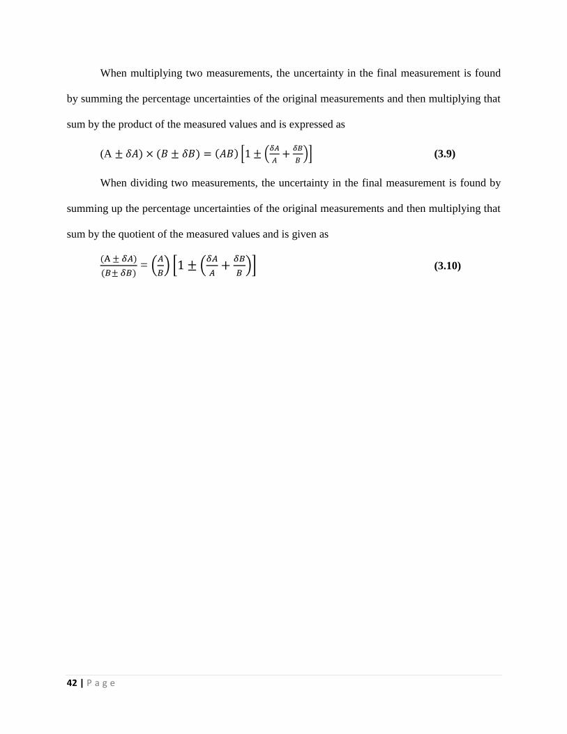
42 | P a g e

When multiplying two measurements, the uncertainty in the final measurement is found

by summing the percentage uncertainties of the original measurements and then multiplying that

sum by the product of the measured values and is expressed as

(A ± 𝛿𝐴) × (𝐵 ± 𝛿𝐵) = (𝐴𝐵) [1 ± (𝛿𝐴

𝐴+

𝛿𝐵

𝐵)] (3.9)

When dividing two measurements, the uncertainty in the final measurement is found by

summing up the percentage uncertainties of the original measurements and then multiplying that

sum by the quotient of the measured values and is given as

(A ± 𝛿𝐴)

(𝐵± 𝛿𝐵) = (

𝐴

𝐵) [1 ± (

𝛿𝐴

𝐴+

𝛿𝐵

𝐵)] (3.10)

43 | P a g e

44 | P a g e

4. REGRESSION ANALYSIS

4.1 Introduction

Calorific value is one of the most significant aspects in the selection of a solid fuel and the

designing of the boiler assisting biomass combustion depends upon the calorific value of the

biomass. It can be determined by both experimental methods as well as analytical methods. The

experimental methods are already discussed in the previous chapter. The calorific value is

determined experimentally by a calorimeter which needs special skills to operate and consumes a

lot of time [56]. But in case of analytical method, regression equations were developed to

determine gross calorific value (GCV) from the data of proximate and ultimate analyses without

conducting any fresh experiments. Considering proximate analysis, regression equation for GCV

has been expressed as the function of variables such as moisture content, ash content, volatile

matter content and fixed carbon content [57]. Similarly, from the data of ultimate analysis, GCV

has been expressed as the function of variables such as carbon, hydrogen, oxygen and nitrogen

[58]. For this project work, the above expressions have been established on the basis of

regression analysis with the help of Statistica software of version 9.1.

4.2 Regression Analysis

Regression analysis is a statistical technique to analyze the variables and to determine the

relationship between the dependent and independent variables. In general, it is used to predict

and forecast the regression function. Usually, the known values of dependent and independent

variables are utilized to develop an equation called regression equation [59].

On the basis of the number of independent variables, regression analysis can be classified

into two broad categories i.e., Simple Regression Analysis (SRA) and Multiple Regression

45 | P a g e

Analysis (MRA). There is only one independent variable in SRA whereas MRA has more than

one. On the basis of the relationship between dependent and independent variables, regression

analysis can be classified into two groups such as, Linear Regression Analysis and Nonlinear

Regression Analysis. The relationship between dependent and independent variables can be

direct or inverse. Direct relationship shows increase in dependent variable with the increase in

independent variable displaying a positive slope in the graph. On the other hand in inverse

relationship, the dependent variable decreases with the increase in independent variable and the

slope is negative [60].

4.3 Linear Regression Analysis

Linear regression analysis is a statistical approximation in which a dependent or

explained variable is linearly related to one or more independent or explanatory variables. In

linear regression, the linear prediction functions are used to model the data and using this, the

unknown model parameters are estimated. The least square approach is most widely used to fit

linear regression models.

4.3.1 Simple linear regression analysis

Simple Linear Regression Analysis (SLRA) is a statistical technique which is used to

estimate the linear relationship between the dependent variable and the single independent

variable. Mathematically, it is expressed as [61]:

Y = ao + a1 X (4.1)

where, Y = dependent or explained variable,

X = independent or explanatory variable and

46 | P a g e

a0, a1 = constant parameters.

4.3.2 Multiple linear regression analysis

Multiple Linear Regression Analysis (MLRA) is used to approximate the relationship

between two or more independent variables and one dependent variable by fitting a linear

equation. MLRA can be expressed mathematically as shown in Equation 4.2 [60].

Y = ao + a1X1 + a2X2 +…+ anXn (4.2)

where ao, a1, a2 …. an are constant parameters.

4.4 Parameters of Regression Analysis

4.4.1 Standard error of estimate

The standard error of the estimate is a measure of the accuracy and reliability of the predicted

equations. It has properties analogous to those of standard deviation. The standard deviation

gives the dispersion of a set of observations about their mean whereas the standard error of

estimate measures the variability of the observed values around the regression line. The standard

error of estimate is expressed by the following formula [60]:

S = √∑(Y− Y )2

N−k−1 (4.3)

where, Y = sample values of dependent variable,

Y= corresponding estimated values from the regression equation,

N = number of data points in the sample, and

k = number of independent variables.

47 | P a g e

4.4.2 Coefficient of determination

In regression analysis, the coefficient of determination is a statistical measure of how well

the regression line approximates the real data points. It provides information about the goodness

of fit of a model. It is a statistic used in the context of statistical models whose main purpose is

either the prediction of future outcomes or the testing of hypotheses, on the basis of other related

information. It provides a measure of how well observed outcomes are replicated by the model,

as the proportion of total variation of outcomes explained by the model. It is denoted by R2.

Mathematically,

R2 = 1- ∑(Y−Y)2

∑(Y− Y)2 (4.4)

where, ∑(Y − Y)2 = variation of the Y value around the regression line

∑(Y − Y)2 = variation of Y values around their own mean

The higher value of R2 suggests that the model developed is more useful and it takes values

between 0 and 1. When R2 takes the value 1, this implies that every data point lies on the

regression line, suggesting perfect correlation between dependent and independent variables. On

the other hand, when R2 takes the value 0, no data point lies on the regression line indicating no

correlation between dependent and independent variables [60].

48 | P a g e

4.4.3 Coefficient of correlation

The coefficient of correlation measures the strength and direction of a linear relationship

between two variables. It is denoted by R. It is also called Pearson product-moment correlation

coefficient. It takes values between −1 and +1, where 1 is total positive correlation, 0 is no

correlation, and −1 is total negative correlation. As compared to R2 the coefficient of correlation

is more difficult to interpret, it is usually considered for the evaluation of regression equations

[60].

4.5 Evaluation of Errors

The evaluation of error is essential as it indicates the goodness of the developed model. To

evaluate the accuracy of the developed equations, two statistical parameters, i.e., average bias

error (ABE) and average absolute error (AAE) were used [62]. Mathematically,

ABE = 1

N ∑ [

Predicted value−Measured value

Measured value] × 100%N

i=1 (4.5)

AAE = 1

N ∑ |

Predicted value−Measured value

Measured value| × 100%N

i=1 (4.6)

where, N = number of data points.

AAE quantifies how close the predicted values are to the experimental values in which lower

AAE indicates higher accuracy. For ABE, a positive value indicates an overall over-estimation

while a negative value indicates an overall under-estimation. The smaller the value of ABE, the

smaller the bias of the correlation [48].

49 | P a g e

50 | P a g e

5. RESULTS AND DISCUSSION

5.1 Introduction

The results obtained from the proximate and ultimate analyses, bulk densities, calorific

values and ash fusion temperatures of selected agricultural residues have been outlined in Tables

5.1-5.7. The regression analysis has also been done on the basis of proximate and ultimate

analyses data and the equations developed for gross calorific values are shown in Tables 5.13

and 5.14.

5.2 Chemical Compositions of the Studied Biomass Species

5.2.1 Proximate analysis

The knowledge of the proximate analysis of the selected agricultural residues is vital as it

provides an approximate idea about the energy values and extent of pollutant emission during

their combustion. The freshly cut biomass species contains a large amount of free moisture

which needs to be removed in order to decrease the cost of transportation and increase the

calorific value. The proximate analysis of different components of the selected biomass species

are presented in Table 5.1.

From Table 5.1, it can be observed that moisture content of palm leaf is highest (i.e., 12

wt.%) among all the selected biomass species whereas the stem of banana plant exhibited lowest

moisture content (i.e., 5 wt.%). The presence of high moisture content in the biomass is expected

to reduce the overall thermal efficiency and increase the energy consumption during combustion

in boiler operation. Moreover, the transportation becomes less efficient and the energy value of

biomass with high moisture content is low. Hence, the moisture content of the biomass should be

removed before utilizing it for power generation. Table 5.1 shows that the ash content in the

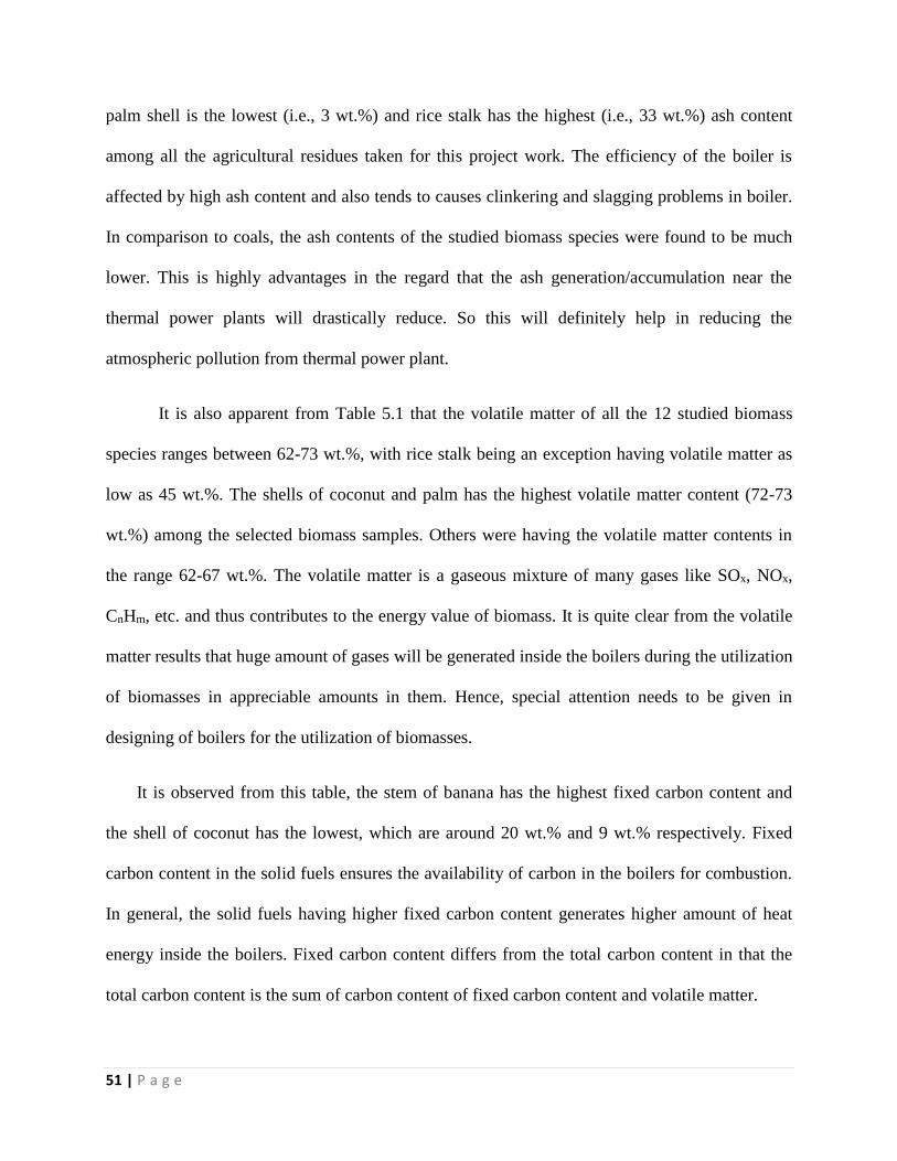
51 | P a g e

palm shell is the lowest (i.e., 3 wt.%) and rice stalk has the highest (i.e., 33 wt.%) ash content

among all the agricultural residues taken for this project work. The efficiency of the boiler is

affected by high ash content and also tends to causes clinkering and slagging problems in boiler.

In comparison to coals, the ash contents of the studied biomass species were found to be much

lower. This is highly advantages in the regard that the ash generation/accumulation near the

thermal power plants will drastically reduce. So this will definitely help in reducing the

atmospheric pollution from thermal power plant.

It is also apparent from Table 5.1 that the volatile matter of all the 12 studied biomass

species ranges between 62-73 wt.%, with rice stalk being an exception having volatile matter as

low as 45 wt.%. The shells of coconut and palm has the highest volatile matter content (72-73

wt.%) among the selected biomass samples. Others were having the volatile matter contents in

the range 62-67 wt.%. The volatile matter is a gaseous mixture of many gases like SOx, NOx,

CnHm, etc. and thus contributes to the energy value of biomass. It is quite clear from the volatile

matter results that huge amount of gases will be generated inside the boilers during the utilization

of biomasses in appreciable amounts in them. Hence, special attention needs to be given in

designing of boilers for the utilization of biomasses.

It is observed from this table, the stem of banana has the highest fixed carbon content and

the shell of coconut has the lowest, which are around 20 wt.% and 9 wt.% respectively. Fixed

carbon content in the solid fuels ensures the availability of carbon in the boilers for combustion.

In general, the solid fuels having higher fixed carbon content generates higher amount of heat

energy inside the boilers. Fixed carbon content differs from the total carbon content in that the

total carbon content is the sum of carbon content of fixed carbon content and volatile matter.

52 | P a g e

Table 5.1: Proximate Analysis of Different Components of Studied Biomass Species

Samples Proximate analysis (wt.%, dry basis)

Moisture

content

Ash content Volatile matter Fixed carbon

content

Banana

Leaf 6 17 63 14

Stem 5 10 65 20

Coconut

Leaf 6 16 67 11

Shell 9 9 73 9

Pith 8 11 64 17

Arecanut

Leaf 8 16 66 10

Coir 9 9 64 18

Wheat

Stalk 11 6 65 18

Palm

Leaf 12 6 65 17

Shell 8 3 72 17

Rice

Stalk 10 33 45 12

Husk 7 19 62 12

53 | P a g e

5.2.2 Ultimate analysis

The ultimate analysis gives an idea about the chemical elements (carbon, hydrogen, nitrogen,

sulphur, and oxygen) and ash content of a carbonaceous material. This analysis provides the

composition of the sample which is important to define the energy content, and to determine how

clean and efficient the sample is for the purpose it is used for. The results obtained from the

ultimate analysis of nine different samples of selected agricultural residues have been reported in

Table 5.2. From the ultimate analysis results, one can determine gross calorific value of the

concerned solid fuel by using the Dulong and Petit’s formula which is as follows [63]:

𝐺𝐶𝑉 = 1

100[ 8080 × 𝐶 + 34500 ( 𝐻 −

𝑂

8 ) + 2200 × 𝑆 (5.1)

where, C, H, O and S are the weight percentage of carbon, hydrogen, oxygen and sulphur

content contents in the sample.

The carbon and hydrogen contents of coconut leaf have been found out to be the highest

among all the studied biomass species i.e., 45.456 and 5.656 wt.% respectively as evident from

Table 5.2. On the other hand, the carbon and hydrogen contents of the rice stalk has been

reported to be the lowest i.e., 24.826 and 3.381 wt.% respectively. Rest of the samples have

carbon and hydrogen contents in the range 35-44 wt.% and 3.3-5.5 wt.% respectively.

The oxygen content of coconut pith has been found out to be 40.958 wt.% which is the

highest among all the selected samples and rice stalk with oxygen content of 21.310 wt.% has the

lowest. The other components have oxygen content in the range 31-39 wt.%. The oxygen present

in the sample helps in its combustion in the boiler. The table also shows that the nitrogen content

in the studied samples is in the range 0 - 4.725 wt.%, with wheat stalk being reported to have the

54 | P a g e

highest value. The nitrogen contents of both shell and pith of coconut were found to be zero

which shows that nitrogen content barely affects the gross calorific value.

Table 5.2: Ultimate Analysis of Different Components of Studied Biomass Species

Samples Ultimate analysis (wt. %, dry basis)

Carbon Hydrogen Oxygen Nitrogen

Banana

Stem 35.351 4.162 36.334 1.142

Coconut

Leaf 45.456 5.656 37.146 0.839

Shell 43.996 4.799 38.699 0

Pith 37.497 4.605 40.958 0

Arecanut

Leaf 41.755 5.499 34.725 2.240

Wheat

Stalk 37.899 5.413 38.988 4.725

Palm

Leaf 43.598 5.381 37.366 1.200

Rice

Stalk 24.826 3.381 21.310 1.687

Husk 37.357 5.269 31.463 2.208

55 | P a g e

5.3 Calorific Value

Power generation potential of any energy source can be estimated on the basis of its calorific

value. The knowledge of calorific value helps in depicting the quality of fuel required for power

production. That is why the calorific value of any fuel source is an important criterion for its

selection in power plants. The results obtained for the gross calorific values of the studied

biomass samples have been listed in Table 5.3.

It is evident from Table 5.3 that the leaf of coconut has the highest calorific value and the

stalk of rice has the lowest among all the selected biomass samples which are 19.763 MJ/kg and

14.242 MJ/kg respectively. It is quite clear from the literature that the carbon and hydrogen are

the major elements that affect the gross calorific value. The variations in gross calorific value of

the studied biomass species, as can be seen in Table 5.3, are undoubtedly related to the combined

effects of their carbon and hydrogen contents. For example, it can be seen in Table 5.2 that the

highest gross calorific value of the coconut leaf is due to its highest carbon and hydrogen

contents, and the lowest gross calorific value of rice stalk is due to its lowest carbon and

hydrogen contents. In addition, the carbon and hydrogen contents give an idea about the

availability of combustibles in a boiler.

56 | P a g e

Table 5.3: Calorific Values of Different Components of Studied Biomass Species

Sl. No Sample Gross Calorific Value

(MJ/kg)

1 Banana Leaf 17.406

2 Banana Stem 17.523

3 Coconut Leaf 19.763

4 Coconut Shell 18.898

5 Coconut Pith 17.124

6 Arecanut Leaf 17.879

7 Arecanut Coir 16.565

8 Wheat Stalk 16.605

9 Palm Leaf 17.752

10 Palm Shell 18.155

11 Rice Stalk 14.242

12 Rice Husk 16.872

5.4 Ash Fusion Temperatures

Ash fusion temperatures (AFTs) of six selected agricultural residues viz., stalks of rice and

wheat, rice husk, coconut pith and leaves of arecanut and palm were measured. The results

obtained for the four fusion temperatures (i.e., initial deformation temperature (IDT), softening

temperature (ST), hemispherical temperature (HT) and flow temperature (FT)) of the studied

biomass species have been tabulated in Table 5.4.

57 | P a g e

From the AFT results listed in Table 5.4, it is evident that IDT and ST values of the studied

ash samples are in the range 938-1137 0C and 1083-1211 0C respectively, whereas the values of

HT and FT are in the range of 1151-1281 0C and 1194-1339 0C respectively. Among all types of

fusion temperatures, the lowest is observed to be 938 0C (i.e., for the stalk of rice) which is

substantially above the normal boiler temperature (i.e., 800 0C). This gives an indication that all

the selected biomass samples can be used for combustion in boiler safely without clinker

formation.

AFT is one of the important criteria to be taken in consideration while selecting a solid fuel

for combustion in boilers. AFTs give an idea about the possibility of clinker formation inside the

boilers and other ash related problems like damage of the refractory walls. Out of the four

characteristics ash fusion temperatures, the value of initial deformation temperature is considered

to be the most important in selection of solid fuels for application in boilers.

Table 5.4: Ash Fusion Temperatures of Different Biomass Samples

Biomass

samples

Ash fusion temperatures, 0C

IDT ST HT FT

Rice Stalk 938 1096 1198 1242

Wheat Stalk 996 1083 1151 1265

Rice Husk 1075 1211 1281 1339

Coconut Pith 978 1086 1156 1194

Arecanut leaf 1058 1128 1246 1274

Palm Leaf 1137 1192 1227 1254

58 | P a g e

5.5 Analysis of Co-firing Potentials of Mixed Briquettes of Coal-Selected Biomass Species

The chemical composition and energy values of mixed briquettes of coal-rice husk and coal-

palm leaf of different ratios have been tabulated in Tables 5.5 and 5.6 respectively. From these

tables, it is vivid that there is decrease in ash content and increase in content of volatile matter

for both the coal-biomass mixed samples in contrast to the biomass free coal sample (i.e., coal:

biomass = 100:0) as the percentage of biomass increases in the briquettes. It is evident from the

tables that the mixing of biomass with coal decreases ash content substantially which is an

important criterion in selection of solid fuels as low ash content fuel ensures smooth boiler

operation. Hence, the use of biomass with coal in co-firing process should be considered as it can

help in reduction of emission and bed agglomeration problems.

From the same tables it is evident that, the blending of coal with biomass also affects the

calorific value. In case of coal and rice husk mixed briquette sample, the calorific value

increased when the briquette sample was taken in the ratio 90:10 but it decreased when the

briquette sample was taken in the ratio 85:15. On the other hand, all the coal and palm leaf mixed

briquette samples exhibited an increase in calorific value with the increase in percentage of palm

leaf in the briquette samples. The briquette sample with coal and palm leaf mixed in the ratio

85:15 was found to have the highest calorific value (i.e., 18.213 MJ/kg) among all the biomass

samples studied in different ratios for analysing co-firing potentials.

59 | P a g e

Table 5.5: Proximate Analysis and Gross Calorific Values of Coal-Biomass (Rice husk) Mixed

Briquette in Different Ratios

Ratio

(coal :

biomass)

Proximate analysis (wt.% dry basis)

Gross calorific

value

(MJ/kg)

Moisture Ash Volatile

matter

Fixed carbon

100 : 0 5 38 22 35 17.292

90 : 10 6 30 27 37 17.624

85 : 15 4 28 32 36 17.016

Table 5.6: Proximate Analysis and Gross Calorific Values of Coal-Biomass (Palm leaf) Mixed

Briquette in Different Ratios

Ratio

(coal :

biomass)

Proximate analysis (wt.% dry basis

Gross calorific

value

(MJ/kg)

Moisture Ash Volatile

matter

Fixed carbon

100 : 0 5 38 22 35 17.292

90 : 10 6 29 28 37 17.672

85 : 15 7 28 30 35 18.213

60 | P a g e

5.6 Bulk Density

The study of bulk density of solid fuel is important for its utilization in power generation

through the boiler route as it gives an idea about the amount of solid carbonaceous material to be

accommodated in a given volume of the boiler. Higher bulk density facilitates the

accommodation of large amount of carbonaceous material in a given volume of the boiler. Not

only this, higher bulk densities of solid fuels reduces their cost of transportation and handling.

The bulk density of rice husk has been found out to be the highest (i.e., 336.257 kg/m3)

and that of palm shell is the lowest (i.e., 108.673 kg/m3) among all the studied biomass samples

as seen from Table 5.7. Other biomass samples have been found to be in the range 120 to 297

kg/m3.

61 | P a g e

Table 5.7: Bulk Density of Selected Biomass Species

Sl. No Sample Bulk Density

(kg/𝒎𝟑)

1 Banana Leaf 175.925

2 Banana Stem 120.370

3 Coconut Leaf 296.290

4 Coconut Shell 164.814

5 Coconut Pith 173.611

6 Arecanut Leaf 248.015

7 Arecanut Coir 187.982

8 Wheat Stalk 174.359

9 Palm Leaf 223.784

10 Palm Shell 108.673

11 Rice Stalk 156.364

12 Rice Husk 336.257

5.7 Determination of Uncertainty

Uncertainty in measurements of proximate analyses, gross calorific values and bulk

density have been calculated and presented in Tables 5.8 – 5.12. Considering all the three

readings recorded from the experiments for all the properties, uncertainties in measurements

were calculated.

62 | P a g e

Banana stem has been taken as sample for showing the calculation of uncertainty in

measurement of moisture content as shown below.

Three readings of moisture content in wt. % = 5, 5 and 6.

For these reading, mean (µ) and standard deviation (𝜎) are calculated as

µ =

3

655 = 5.33 ≈ 5

5.0

13

655555222

Considering 95 % confidence level, moisture content in banana stem is found to be 5±2×√0.5 =

5±1.41 wt. %.

The procedure of calculation of uncertainty in measurement of gross calorific value (GCV) of

banana stem was different from that followed in the previous paragraph as GCV involves ratio of

two variable i.e. maximum rise in temperature inside bomb calorimeter (say, A) and weight of

the selected sample (say, B). A sample calculation for determining uncertainty in measurement

of GCV of banana stem has been present.

Three readings of weight of the sample in g = 0.71, 0.73 and 0.75.

Corresponding maximum rise in temperatures in 0C = 1.53, 1.54 and 1.55.

Mean (µ) and standard deviation (𝜎) of these two sets of data were calculated as,

73.0

3

75.073.071.0

B g.

63 | P a g e

02.013

75.073.073.073.071.073.0222

B g.

54.1

3

55.154.153.1

A

0C.

01.013

55.154.154.154.115354.1222

A 0C.

Considering 95 % confidence level,

02.054.101.0254.12 AAAA 0C.

04.073.002.0273.02 BBBB 0C.

Further, using Eq 3.5 and 3.10 uncertainty in measurement of GCV was calculated as follows,

BB

AAEWGCV

..

B

B

A

A

B

A 11987

73.0

04.0

54.1

02.01

73.0

54.11987

= 4191.576 ± 284.141 Kcal/Kg

Converting the gross calorific value into SI units, the uncertainty in measurement of GCV of

banana stem was found to be 17.526 ± 1.188 MJ/Kg.

64 | P a g e

Table 5.8: Uncertainty of Measurement of Proximate Analysis of Different Components of

Studied Biomass Species

Samples Proximate analysis (wt.%, dry basis)

Moisture

content

Ash content Volatile matter Fixed carbon

content

Banana

Leaf 6±2.00 17±0.00 63±4.00 14±2.00

Stem 5±1.41 10±1.41 65±1.41 20±3.16

Coconut

Leaf 6±1.41 16±1.41 67±4.00 11±4.00

Shell 9±1.41 9±2.41 73±3.16 9±2.00

Pith 8±1.41 11±2.00 64±2.00 17±3.16

Arecanut

Leaf 8±2.00 16±1.41 66±4.00 10±3.16

Coir 9±1.41 9±3.16 64±1.41 18±1.41

Wheat

Stalk 11±2.00 6±2.00 65±2.00 18±2.00

Palm

Leaf 12±2.00 6±4.00 65±4.00 17±2.00

Shell 8±1.41 3±1.41 72±3.16 17±3.16

Rice

Stalk 10±4.00 33±4.00 45±2.00 12±2.00

Husk 7±1.41 19±2.00 62±4.00 12±3.16

65 | P a g e

Table 5.9: Uncertainty of Measurement of Gross Calorific Value of Different Components of

Studied Biomass Species

Sl. No Sample Gross Calorific Value

(MJ/kg)

Uncertainty of

Measurement

1 Banana Leaf 17.406 ±1.218

2 Banana Stem 17.523 ±1.188

3 Coconut Leaf 19.763 ±0.483

4 Coconut Shell 18.898 ±0.627

5 Coconut Pith 17.124 ±0.705

6 Arecanut Leaf 17.879 ±0.976

7 Arecanut Coir 16.565 ±0.574

8 Wheat Stalk 16.605 ±0.594

9 Palm Leaf 17.752 ±1.328

10 Palm Shell 18.155 ±1.142

11 Rice Stalk 14.242 ±0.752

12 Rice Husk 16.872 ±0.662

66 | P a g e

Table 5.10: Uncertainty of Measurement of Bulk Density of the Selected Biomass Species

Sl. No Sample Bulk Density

(kg/𝒎𝟑)

Uncertainty of

Measurement

1 Banana Leaf 175.925 ±5.378

2 Banana Stem 120.370 ±2.898

3 Coconut Leaf 296.290 ±2.340

4 Coconut Shell 164.814 ±4.372

5 Coconut Pith 173.611 ±4.786

6 Arecanut Leaf 248.015 ±0.790

7 Arecanut Coir 187.982 ±5.488

8 Wheat Stalk 174.359 ±0.340

9 Palm Leaf 223.784 ±5.602

10 Palm Shell 108.673 ±3.682

11 Rice Stalk 156.364 ±2.496

12 Rice Husk 336.257 ±3.130

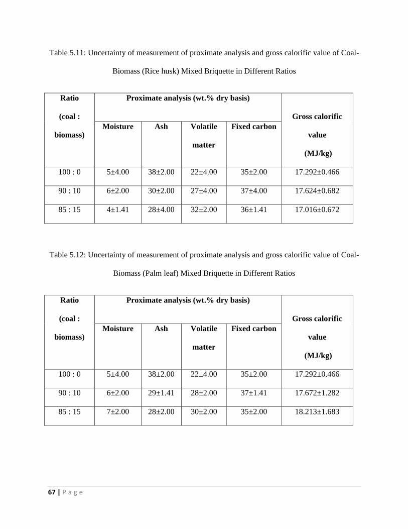
67 | P a g e

Table 5.11: Uncertainty of measurement of proximate analysis and gross calorific value of Coal-

Biomass (Rice husk) Mixed Briquette in Different Ratios

Ratio

(coal :

biomass)

Proximate analysis (wt.% dry basis)

Gross calorific

value

(MJ/kg)

Moisture Ash Volatile

matter

Fixed carbon

100 : 0 5±4.00 38±2.00 22±4.00 35±2.00 17.292±0.466

90 : 10 6±2.00 30±2.00 27±4.00 37±4.00 17.624±0.682

85 : 15 4±1.41 28±4.00 32±2.00 36±1.41 17.016±0.672

Table 5.12: Uncertainty of measurement of proximate analysis and gross calorific value of Coal-

Biomass (Palm leaf) Mixed Briquette in Different Ratios

Ratio

(coal :

biomass)

Proximate analysis (wt.% dry basis)

Gross calorific

value

(MJ/kg)

Moisture Ash Volatile

matter

Fixed carbon

100 : 0 5±4.00 38±2.00 22±4.00 35±2.00 17.292±0.466

90 : 10 6±2.00 29±1.41 28±2.00 37±1.41 17.672±1.282

85 : 15 7±2.00 28±2.00 30±2.00 35±2.00 18.213±1.683

68 | P a g e

5.8 Regression Analysis

The regression analysis has been performed on the data experimentally determined by

proximate analysis, ultimate analysis and gross calorific values in order to develop regression

equations for gross calorific value (GCV) as the function of variables associated with proximate

and ultimate analyses and the findings have been listed in Tables 5.13 and 5.14.

5.8.1 Regression analysis performed on proximate analysis data

As discussed earlier in Section 5.2.1, the volatile matter and fixed carbon contents hugely

affect the calorific value. On the other hand, moisture and ash contents have insignificant effects.

So, these two variables were dropped in subsequent stages while developing regression

equations. First, the moisture content was dropped and the regression equation for calorific value

involving rest of the three variables was developed as follows:

GCV = - 3.114 + 0.124×AC + 0.288×VM + 0.03×FC (5.2)

where, GCV= predicted gross calorific value in MJ/kg

AC = ash content in wt.%

VM = volatile matter content in wt.%,

FC = fixed carbon content in wt.%,

Similarly, the regression equation involving three variables after dropping ash content was

obtained as shown below:

GCV = 9.256 - 0.124×MC + 0.164×VM - 0.094×FC (5.3)

where, MC = the moisture content in wt.%

69 | P a g e

Then, both the moisture and ash contents were dropped and the corresponding equation

involving fixed carbon and volatile matter was found to be

GCV = 7.902 + 0.171×VM - 0.101×FC (5.4)

Out of these two contents taking one at a time, two more regression were developed as

follows:

GCV= 6.619 + 0.168×VM (5.5)

GCV= 18.614 - 0.083×FC (5.6)

The statistical performance measures such as R-squared value (R2), R value (R), standard

error of estimate (S), average bias error (ABE) and average absolute error (AAE) for all the

above regression relationships shown in Equations 5.2-5.6 have been computed and listed in

Table 5.13.

70 | P a g e

Table 5.13: Developed Regression Equations for the Estimation of the Gross Calorific Values of

Studied Biomass Samples from Proximate Analysis Data and Their Statistical Performance

Measures

Eq.

No.

Regression equation R-

squared

value

(R2)

R value

(R)

Standard

error of

estimate

(S)

Average

bias

error

(ABE)

(in %)

Average

absolute

error

(AAE)

(in %)

5.2 GCV= - 3.114 + 0.124×AC +

0.288×VM + 0.03×FC

0.834 0.913 0.651 0.086 2.15

5.3 GCV= 9.256 - 0.124×MC +

0.164×VM - 0.094×FC

0.833 0.912 0.651 0.085 2.15

5.4 GCV= 7.902 + 0.171×VM -

0.101×FC

0.799 0.894 0.674 0.106 2.522

5.5 GCV= 6.619 + 0.168×VM 0.725 0.852 0.748 0.140 2.454

5.6 GCV= 18.614 - 0.083×FC 0.051 0.224 1.392 0.579 5.272

Table 5.13 shows that R2 values of the Equations 5.2-5.4 has been found to be higher

than 0.8 which suggests the existence of a strong correlation between GCV and independent

variables. All these three equations have low values of standard error of estimate S (i.e., 0.651-

0.674) which indicates smaller deviation of data points from the regression line. The lower

values AAE of these three equations suggest less error in predicting GCV and more close to the

71 | P a g e

measured value of GCV. Further, as all the ABE values are positive the predictions of GCV are

over-estimated and the values are low i.e., within 0.106 for these three equations.

Equation 5.5 shows a moderate value of R2 (i.e., 0.725) suggesting average correlation

between volatile matter and GCV. The standard error of estimate of this equation was found to

be 0.748 which indicates deviation of some data points from the regression line. Further, AAE

for this equation was found to be 2.454, suggesting some error in predicted GCV and positive

values of ABE suggests that GCV is over-estimated by a margin 0.140. On the other hand,

Equation 5.6 has a very low value of R2 (i.e., 0.051) suggesting a weak correlation of fixed

carbon FC upon GCV. This equation have higher values of standard errors of estimate (i.e.,

1.392), indicating more deviation of data points from the regression line. Further, high AAE

indicates more error in GCV and high positive values of ABE suggests that GCV is over-

estimated by a margin 0.579.

Therefore, with higher R2 value, lower S value and lower percentage of errors in terms of

ABE or AAE, Equations 5.2-5.4 can be considered for prediction of GCV. Out of all regression

equations developed, Equation 5.2 have been found to be the best with the highest R2 value

(0.834), lowest S value (0.651), and low values of ABE (0.086) and AAE (2.15). Hence, this

regression equation should be considered to predict GCV.

5.8.2 Regression analysis performed on ultimate analysis data

All the four variables associated with ultimate analysis have been considered for developing

regression equations for gross calorific value (GCV). Initially, equation for GCV was developed

considering all the four variables i.e., O, N, C and H and the corresponding regression equation

developed was:

72 | P a g e

GCV= 9.412 + 0.286×C - 0.555×H – 0.006×O – 0.078×N (5.7)

As discussed earlier in Section 5.2.2, the calorific value of a solid fuel is not significantly

affected by oxygen and nitrogen contents, hence these variables were dropped one by one and

then both in the subsequent stages. Regression equations considering one variable at a time i.e.,

C or H were also developed. All these regression equations established for GCV are as follows:

GCV= 9.412 + 0.316×C - 0.787×H – 0.01×O (5.8)

GCV= 9.361 + 0.279×C - 0.527×H – 0.085×N (5.9)

GCV= 9.322 + 0.307×C – 0.774×H (5.10)

GCV= 8.543 + 0.229×C (5.11)

GCV= 10.577 + 1.391×H (5.12)

where, GCV = predicted gross calorific value in MJ/kg

C = carbon in wt.%

H = hydrogen wt.%

O = oxygen in wt.%

N = nitrogen wt.%.

The statistical performance measures such as, R-squared value (R2), R value (R), standard

error of estimate (S), average bias error (ABE) and average absolute error (AAE) for all the

above regression relationships have been computed and tabulated in Table 5.14.

73 | P a g e

Table 5.14: Developed Regression Equations for the Estimation of the Gross Calorific Values of

Studied Biomass Samples from Ultimate Analysis Data and Their Statistical Performance

Measures

Eq.

No.

Developed equation R-

squared

value

(R2)

R

value

(R)

Standard

error of

estimate

(S)

Average

bias

error

(ABE)

(in %)

Average

absolute

error

(AAE)

(in %)

5.7 GCV= 9.412 + 0.286×C -

0.555×H – 0.006×O –

0.078×N

0.907 0.952 0.666 0.061 1.796

5.8 GCV= 9.412 + 0.316×C -

0.787×H – 0.01×O

0.905 0.951 0.601 0.063 1.862

5.9 GCV= 9.361 + 0.279×C -

0.527×H – 0.085×N

0.907 0.952 0.596 0.061 1.804

5.10 GCV= 9.322 + 0.307×C –

0.774×H

0.905 0.951 0.550 0.061 1.886

5.11 GCV= 8.543 + 0.229×C 0.864 0.929 0.609 0.087 2.395

5.12 GCV= 10.577 + 1.391×H 0.456 0.675 1.219 0.391 5.441

74 | P a g e

From Table 5.14 it can be observed that, R2 values of the Equations 5.7-5.10 have been found

to be higher than 0.9 which suggests the existence of a strong correlation of the independent

variables upon GCV. All these four equations have low values of standard error of estimate S

(i.e., 0.550-0.666) which indicates smaller deviation of data points from the regression line. The

lower values of AAE of these four equations suggest less error in predicting GCV and more

close to the measured value of GCV. Further as all the ABE values are positive, the predictions

of GCV are over-estimated and the values are low i.e., within 0.063 for all these four equations.

In case of Equation 5.12, R2 value has been found to be 0.456 suggesting a weak correlation

between H and GCV, when H was considered as single independent variable. The high values

standard errors of estimate (i.e., 1.219) of this equation indicate more deviation of data points

from the regression line. Further, higher values of AAE indicate more error in GCV and positive

values of ABE suggests that the predicted GCV is over-estimated by a margin of 0.391.

Therefore, with higher R2 value, lower S value and lower percentage of errors in terms of

ABE or AAE, Equations 5.7-5.10 can be considered for prediction of GCV. Out of all regression

equations developed, Equation 5.7 has been found out to be the best with the highest R2 value

(0.907), lower S value (0.666), and lower values of ABE (0.061) and AAE (1.796). Hence, this

regression equation should be considered to predict GCV.

5.9 An Approach for Decentralized Power Generation and Energy Plantation Structure

A cluster of 10-12 villages consisting of nearly 2000 families was considered to assess

the electricity requirement and one power plant can be designed accordingly. Approximately 2

kWh/day is the electricity requirement per family for domestic purposes [64]. Considering an

additional 11000 kWh/day (approx.) of energy for irrigational purposes and small-scale

75 | P a g e

industries around the villages, a power plant should be designed which can generate 15 MWh

(i.e., 2 x 2000 + 11000) of electricity per day which is same as 5475 MWh/year (i.e., 15 x 365).

5.9.1 Land requirement for biomass

The rates of production of different components of selected agricultural biomass species viz.,

banana, coconut, arecanut, palm, wheat and rice in tonnes per hectare (i.e., t/ha) on dry basis

were obtained from field studies and are shown in Tables 5.15-5.20. The gross calorific values in

MJ/kg of these components shown in Table 5.3 were converted into MJ/t and are listed in these

tables. The energy content (i.e., in MJ/ha) of different residual components of selected

agricultural species as listed in these tables, was found out by multiplying the gross calorific

value (i.e., in MJ/t) with the amount of residues produced per hectare (i.e., in t/ha).

Table 5.15: Total Energy Contents and Power Generation Structure for Banana

Component Gross Calorific

value (MJ/t, dry

basis)

Biomass production

(t/ha, dry basis)

Energy content

(MJ/ha)

Leaf 17.406 × 103 0.91 15.839 × 103

Stem 17.523 × 103 0.09 1.577 × 103

76 | P a g e

Table 5.16: Total Energy Contents and Power Generation Structure from Coconut Biomass

Species

Component Gross Calorific

value (MJ/t, dry

basis)

Biomass production

(t/ha, dry basis)*

Energy content

(MJ/ha)

Shell 18.898 × 103 5.00 94.490 × 103

Pith 17.124 × 103 2.50 42.810 × 103

Leaf 19.763 × 103 1.34 26.482 × 103

Table 5.17: Total Energy Contents and Power Generation Structure from Arecanut Biomass

Species

Component Gross Calorific

value (MJ/t, dry

basis)

Biomass production

(t/ha, dry basis)

Energy content

(MJ/ha)

Leaf 17.879 × 103 0.55 9.784 × 103

Coir 16.565 × 103 2.36 39.093 × 103

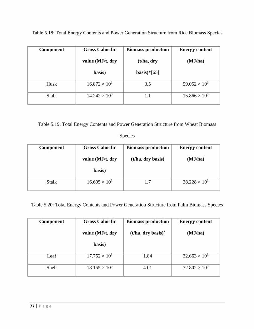
77 | P a g e

Table 5.18: Total Energy Contents and Power Generation Structure from Rice Biomass Species

Component Gross Calorific

value (MJ/t, dry

basis)

Biomass production

(t/ha, dry

basis)*[65]

Energy content

(MJ/ha)

Husk 16.872 × 103 3.5 59.052 × 103

Stalk 14.242 × 103 1.1 15.866 × 103

Table 5.19: Total Energy Contents and Power Generation Structure from Wheat Biomass

Species

Component Gross Calorific

value (MJ/t, dry

basis)

Biomass production

(t/ha, dry basis)

Energy content

(MJ/ha)

Stalk 16.605 × 103 1.7 28.228 × 103

Table 5.20: Total Energy Contents and Power Generation Structure from Palm Biomass Species

Component Gross Calorific

value (MJ/t, dry

basis)

Biomass production

(t/ha, dry basis)*

Energy content

(MJ/ha)

Leaf 17.752 × 103 1.84 32.663 × 103

Shell 18.155 × 103 4.01 72.802 × 103

78 | P a g e

Calculation for Land Requirement for Energy Plantation

The thermal efficiency of biomass fuelled heat engine and the overall efficiency of the power

plant have been considered as 27 % and 85 % respectively. Using the values of energy contents

shown in Tables 5.15-5.20, calculations have been done to find out land required in hectares for

energy plantation in order to have continuous generation of electricity at the rate of 5475

MWh/year. A sample calculation for coconut plant has been shown in next paragraph.

Sample calculation for land requirement for coconut plant

Adding the energy contents of all the waste components obtained from coconut plant, the total

energy available per hectare of land is obtained as (94.490 + 42.810 + 26.482) × 103 MJ/ha =

163.78 × 103 MJ/ha.

Energy output from coconut biomass from one hectare of land considering 27 % thermal

efficiency = 163.78 × 103 × 0.27 = 44221.14 MJ = 44221.14 × 0.0002777778 = 12.28365 MWh.

Power generation considering 85 % overall efficiency = 12.28365 × 0.85 = 10.441103 MWh/ha.

Therefore, land required to supply electricity from coconut biomass species for the whole year =

5475

10.441103 = 524.37 hectares ≡ 524 hectares.

The above procedure was followed to calculate land required for energy plantation for the

rest of the selected agricultural biomass species and the results have been outlined in Table 5.21.

79 | P a g e

Table 5.21: Land Required for Energy Plantation of Different Agricultural Biomass Species for

generating 15 MWh per day

Sl. No. Biomass Species Land Required (ha)

1. Banana 4931

2. Coconut 524

3. Arecanut 1757

4. Palm 814

5. Wheat 3043

6. Rice 1146

5.9.2 Fuel Requirement for co-firing with biomass

Power generation structure for briquettes of coal made by mixing with rice husk and also

with palm leaf in different ratios was developed. Referring Tables 5.5-5.6, the gross calorific

values in MJ/kg of the briquettes were converted to MJ/t and shown in Tables 5.22 and 5.23 for

both the biomass species.

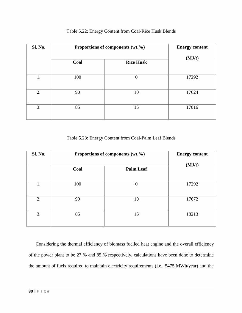
80 | P a g e

Table 5.22: Energy Content from Coal-Rice Husk Blends

Sl. No. Proportions of components (wt.%) Energy content

(MJ/t) Coal Rice Husk

1. 100 0 17292

2. 90 10 17624

3. 85 15 17016

Table 5.23: Energy Content from Coal-Palm Leaf Blends

Sl. No. Proportions of components (wt.%) Energy content

(MJ/t) Coal Palm Leaf

1. 100 0 17292

2. 90 10 17672

3. 85 15 18213

Considering the thermal efficiency of biomass fuelled heat engine and the overall efficiency

of the power plant to be 27 % and 85 % respectively, calculations have been done to determine

the amount of fuels required to maintain electricity requirements (i.e., 5475 MWh/year) and the

81 | P a g e

results have been outlined in Tables 5.24-5.25. The sample calculation of fuel requirement for

coal-rice husk mixed briquette has been shown below for various ratios.

a) Amount of fuel required when proportion of coal-rice husk is 100:0 (i.e., 100 % coal)

Referring Table 5.22, energy content of briquette made of 100% coal = 17292 MJ/t

Total work output from 1 tonne of coal at 27 % of thermal efficiency of biomass fuelled heat

engine = 17292 × 0.27 = 4668.84 MJ/t.

Total electricity generated considering 85 % overall efficiency of a thermal power plant =

4668.84 × 0.85 = 3968.51 MJ/t = 3968.51 × 0.00027777778 MWh/t = 1.102 MWh/t

Thus, the amount of coal required to supply electricity of 5475 MWh for the whole year =

5475 MWh/year

1.102 MWh/t = 4968.24 t/year ≡ 4968 t/year.

b) Amount of fuel required when proportion of coal-rice husk is 90:10 (i.e., 90 % coal and 10 %

rice husk)

Referring Table 5.22, energy content of briquette made of 90 % coal and 10 % rice husk = 17624

MJ/t

Total work output from 1 tonne of coal-rice husk briquette at 27 % of thermal efficiency of

biomass fuelled heat engine = 17624 × 0.27 = 4758.48 MJ/t.

Total electricity generated considering 85 % overall efficiency of a thermal power plant =

4758.48 × 0.85 = 4044.71 MJ/t = 4044.71 × 0.00027777778 MWh/t = 1.124 MWh/t.

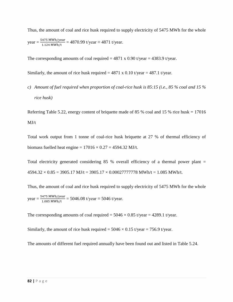
82 | P a g e

Thus, the amount of coal and rice husk required to supply electricity of 5475 MWh for the whole

year = 5475 MWh/year

1.124 MWh/t = 4870.99 t/year ≡ 4871 t/year.

The corresponding amounts of coal required = 4871 x 0.90 t/year = 4383.9 t/year.

Similarly, the amount of rice husk required = 4871 x 0.10 t/year = 487.1 t/year.

c) Amount of fuel required when proportion of coal-rice husk is 85:15 (i.e., 85 % coal and 15 %

rice husk)

Referring Table 5.22, energy content of briquette made of 85 % coal and 15 % rice husk = 17016

MJ/t

Total work output from 1 tonne of coal-rice husk briquette at 27 % of thermal efficiency of

biomass fuelled heat engine = 17016 × 0.27 = 4594.32 MJ/t.

Total electricity generated considering 85 % overall efficiency of a thermal power plant =

4594.32 × 0.85 = 3905.17 MJ/t = 3905.17 × 0.00027777778 MWh/t = 1.085 MWh/t.

Thus, the amount of coal and rice husk required to supply electricity of 5475 MWh for the whole

year = 5475 MWh/year

1.085 MWh/t = 5046.08 t/year ≡ 5046 t/year.

The corresponding amounts of coal required = 5046 × 0.85 t/year = 4289.1 t/year.

Similarly, the amount of rice husk required = 5046 × 0.15 t/year = 756.9 t/year.

The amounts of different fuel required annually have been found out and listed in Table 5.24.

83 | P a g e

Tables 5.24: Fuel Required for Coal-Rice Husk Briquettes

Sl. No. Proportions of Components

(wt. %)

Fuel Required (t/year)

Coal Rice husk Coal Rice husk Total

1. 100 0 4968.0 0 4968

2. 90 10 4383.9 487.1 4871

3. 85 15 4289.1 756.9 5046

Similarly following the above procedure, the amount of fuel required for coal-palm leaf

briquettes was calculated and listed in Table 5.25.

Tables 5.25: Fuel Required for Coal-Palm Leaf Briquettes

Sl. No. Proportions of Components

(wt. %)

Fuel Required (t/year)

Coal Palm leaf Coal Palm leaf Total

1. 100 0 4968.0 0 4968

2. 90 10 4375.8 486.2 4862

3. 85 15 4008.6 707.4 4716

84 | P a g e

Tables 5.24-5.25 show the requirement of coal and biomass in tonnes per year for making

briquettes of coal-rice husk and coal-palm leaf respectively with biomass ratio varying from 0 to

15 % so as to maintain a continuous generation of electricity ate the rate of 5475 MWh/year.

85 | P a g e

86 | P a g e

6. CONCLUSIONS

6.1 Conclusions

Based on the experimental results carried out in this work, the following conclusions can be

summarized.

a) The ash content of rice stalk i.e., 33 wt.% has been found to be the highest among all the

studied samples. This is a matter of concern, as the high values of ash content affects the

efficiency of the boiler, and causes clinkering and slagging problems.

b) The coconut shell has been found to have the highest volatile matter (i.e., 73 wt.%) among

the agricultural wastes studied. A high value of volatile matter contributes towards high value

of its gross calorific value.

c) Banana stem has been reported to have the highest fixed carbon content i.e., 20 wt% among

the studied biomass samples which suggests that it will generate higher amount of heat inside

the boiler.

d) The leaves and shells of coconut have been found to have calorific values (i.e., above 18

MJ/kg) as well as their corresponding carbon (i.e., above 43 wt.%) and hydrogen (i.e., above

4.5 wt.%) contents in the higher range among all the studied samples. Hence, they can also

have significant contribution towards power generation.

e) Initial deformation temperatures (IDTs) of all the studied samples are found to be in the

range 938-1137 0C which is considerably above the safe boiler temperature i.e. around 800

0C. This indicates that all the studied samples can be safely used as solid fuels for

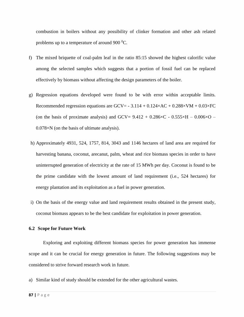
87 | P a g e

combustion in boilers without any possibility of clinker formation and other ash related

problems up to a temperature of around 900 0C.

f) The mixed briquette of coal-palm leaf in the ratio 85:15 showed the highest calorific value

among the selected samples which suggests that a portion of fossil fuel can be replaced

effectively by biomass without affecting the design parameters of the boiler.

g) Regression equations developed were found to be with error within acceptable limits.

Recommended regression equations are GCV= - 3.114 + 0.124×AC + 0.288×VM + 0.03×FC

(on the basis of proximate analysis) and GCV= 9.412 + 0.286×C - 0.555×H – 0.006×O –

0.078×N (on the basis of ultimate analysis).

h) Approximately 4931, 524, 1757, 814, 3043 and 1146 hectares of land area are required for

harvesting banana, coconut, arecanut, palm, wheat and rice biomass species in order to have

uninterrupted generation of electricity at the rate of 15 MWh per day. Coconut is found to be

the prime candidate with the lowest amount of land requirement (i.e., 524 hectares) for

energy plantation and its exploitation as a fuel in power generation.

i) On the basis of the energy value and land requirement results obtained in the present study,

coconut biomass appears to be the best candidate for exploitation in power generation.

6.2 Scope for Future Work

Exploring and exploiting different biomass species for power generation has immense

scope and it can be crucial for energy generation in future. The following suggestions may be

considered to strive forward research work in future.

a) Similar kind of study should be extended for the other agricultural wastes.

88 | P a g e

b) Studies can be made for improving the efficiencies of existing biomass fuelled power plants.

c) In addition to the above, attention of scientists and technocrats needs to be directed towards

improving the yields of biomass per hectare of land.

89 | P a g e

90 | P a g e

References

[1] Raghuvanshi S. P., Chandra A. and Raghav A. K. Carbon dioxide emissions from coal based

power generation in India, Energy Conversion and Management, 47 (2006): pp. 427-441

[2] Ministry of new and renewable energy. Grid interactive and off-grid renewable power, New

Delhi: Government of India, http://mnre.gov.in/file-manager/annual-report/2010-

2011/EN/Chapter%205/chapter%205.htm (2011)

[3] Ministry of Agriculture. Annual Report 2014, http://agricoop.nic.in/Annualreport2013-

14/artp13-14ENG.pdf (2014)

[4] Ministry of Statistics and Programme Implementation. Energy Statistics 2014,

http://mospi.nic.in/mospi_new/upload/Energy_stats_2014.pdf (2014)

[5] Kumar M. and Patel S. K. Energy values and estimation of power generation potentials of

some non-woody biomass species, Energy Sources, Part A: Recovery, Utilization, and

Environmental Effects, 30 (2008): pp. 765-773

[6] Kumar M., Patel S. K. and Mishra S. Studies on characteristics of some shrubaceous non-

woody biomass species and their electricity generation potentials, Energy Sources, Part A:

Recovery, Utilization, and Environmental Effects, 32 (2010): pp. 786-795

[7] International Energy Agency, Key World Energy Statistics,

http://www.iea.org/publications/freepublications/publication/KeyWorld2013.pdf (2013)

[8] Renewable energy policy network for the 21st century, Global Status Report 2012,

www.map.ren21.net/GSR/GSR2012_low.pdf (2012)

[9] Renewable energy policy network for the 21st century, Global Status Report 2013,

http://www.ren21.net/portals/0/documents/resources/gsr/2013/gsr2013_lowres.pdf (2013)

91 | P a g e

[10] Renewable energy policy network for the 21st century, Global Status Report 2014,

www.ren21.net/portals/0/.../2014/gsr2014_full%20report_low%20res.pdf (2014)

[11] India's energy scenario in 2013 - challenges and prospects, Hydrocarbon Asia, (2013): pp.

6-10, http://www.hcasia.safan.com/mag/hcajanmar13/r06.pdf

[12] EPA Combined Heat and Power Partnership,

http://www.epa.gov/chp/documents/biomass_chp_catalog_part5.pdf (2002)

[13] Federal Technology Alert, A new technology demonstration publication,

http://www.nrel.gov/docs/fy04osti/33811.pdf (2004)

[14] Kurchania A. K. Biomass Energy, Chapter 2,

http://www.springer.com/cda/content/document/cda_downloaddocument/9783642284175-c2.pdf

(2014)

[15] Kishore V. V. N. and Mande S. Development benefits of clean energy in India: Biomass

gasification prospects in India, The William and Flora Hewlett Foundation. New Delhi: The

Energy and Resources Institute (2007)

[16] Das B. K. and Hoque S. M. N. Assessment of the potential of biomass gasification for

electricity generation in Bangladesh, Journal of Renewable Energy,

http://dx.doi.org/10.1155/2014/429518 (2014)

[17] Wyman C. E. Ethanol from lignocellulosic biomass: technology, economics, and

opportunities, Bioresource Technology, 50 (1994): pp. 3-15

[18] Biomass Co-firing, IEA-ETSAP and IRENA Technology Brief E21,

http://www.irena.org/DocumentDownloads/Publications/IRENA-

ETSAP%20Tech%20Brief%20E21%20Biomass%20Co-firing.pdf (2013)

92 | P a g e

[19] Ministry of Statistics and Programme Implementation. Energy Statistics 2014.

http://mospi.nic.in/mospi_new/upload/Energy_stats_2014.pdf (2014)

[20] Rastogi C. Changing geo-politics of oil and the impact on India, Procedia-Social and

Behavioral Sciences, 133 (2014): pp. 93-105

[21] Parikh J. and Parikh K. India’s energy needs and low carbon options, Energy, 36 (2011): pp.

3650-3658

[22] Bhattacharya S. and Jana C. Renewable energy in India: historical developments and

prospects, Energy, 34 (2009): pp. 981-991

[23] Blenkinsopp T., Coles S. and Kirwan K. Renewable energy for rural communities in

Maharashtra, India, Energy Policy, 60 (2013): pp. 192-199

[24] Pillai I. R. and Banerjee R. Renewable energy in India: status and potential, Energy, 34

(2009): pp. 970-980

[25] Gera R., Rai H., Parvej Y. and Soni H. Renewable energy scenario in India: opportunities

and challenges, Indian Journal of Electrical and Biomedical Engineering, 1 (2013): pp. 10-16

[26] Werther J., Saenger M., Hartge E. U., Ogada T. and Siagi Z. Combustion of agricultural

residues, Progress in Energy and Combustion Science, 26 (2000): pp. 1-27

[27] Cherubini F. and Ulgiati S. Crop residues as raw materials for biorefinery systems – A LCA

case study, Applied Energy, 87 (2010): pp. 47-57

[28] Chauhan S. Biomass resources assessment for power generation: a case study from Haryana

state, India, Biomass and Bioenergy, 34 (2010): pp. 1300-1308

[29] Chauhan S. District wise agriculture biomass resource assessment for power generation: a

case study from an Indian state, Punjab, Biomass and Bioenergy, 37 (2012): pp. 205-212

93 | P a g e

[30] Williams A., Jones J. M., Ma L. and Pourkashanian M. Pollutants from the combustion of

solid biomass fuels, Progress in Energy and Combustion Science, 38 (2012): pp. 113-137

[31] Cardozo E., Erlich C., Alejo L. and Fransson T. H. Combustion of agricultural residues: an

experimental study for small-scale applications, Fuel, 115 (2014): pp. 778-787

[32] Mukunda H., Dasappa S., Paul P., Rajan N. and Shrinivasa U. Gasifiers and combustors for

biomass–technology and field studies, Energy for Sustainable Development, 1 (1994): pp. 27-38

[33] Küçük M. M. and Demirbaş A. Biomass conversion processes, Energy Conversion and

Management, 38 (1997): pp. 151-165

[34] Chum H. L. and Overend R. P. Biomass and renewable fuels, Fuel Processing Technology,

71 (2001): pp. 187-195

[35] Wander P. R., Altafini C. R. and Barreto R. M. Assessment of a small sawdust gasification

unit, Biomass and Bioenergy, 27 (2004): pp. 467-476

[36] Dixit C. S. B., Paul P. J. and Mukunda H. S. Part I: Experimental studies on a pulverised

fuel stove, Biomass and Bioenergy, 30 (2006): pp. 673-683

[37] Demirbas A. Progress and recent trends in biofuels, Progress in Energy and Combustion

Science, 33 (2007): pp. 1-18

[38] Nussbaumer T. Combustion and co-combustion of biomass: fundamentals, technologies,

and primary measures for emission reduction, Energy and Fuels, 17 (2003): pp. 1510-1521

[39] Fang X. and Jia L. Experimental study on ash fusion characteristics of biomass, Bioresource

Technology, 104 (2012): pp. 769-774

[40] Vamvuka D. and Kakaras E. Ash properties and environmental impact of various biomass

and coal fuels and their blends, Fuel Processing Technology, 92 (2011): pp. 570-581

94 | P a g e

[41] Niu Y., Tan H., Wang X., Liu Z., Liu H., Liu Y. and Xu T. Study on fusion characteristics

of biomass ash, Bioresource Technology, 101 (2010): pp. 9373-9381

[42] Xiao R., Chen X., Wang F. and Yu G. The physicochemical properties of different biomass

ashes at different ashing temperature, Renewable Energy, 36 (2011): pp. 244-249

[43] Hoffmann B. S., Szklo A. and Schaeffer R. An evaluation of the techno-economic potential

of co-firing coal with woody biomass in thermal power plants in the south of Brazil, Biomass

and Bioenergy, 45 (2012): pp. 295-302

[44] Tillman D. A. Biomass cofiring: the technology, the experience, the combustion

consequences, Biomass and Bioenergy, 19 (2000): pp. 365-384

[45] Parikh J., Channiwala S. and Ghosal G. A correlation for calculating elemental composition

from proximate analysis of biomass materials, Fuel, 86 (2007): pp. 1710-1719

[46] Majumder A., Jain R., Banerjee P. and Barnwal J. Development of a new proximate

analysis based correlation to predict calorific value of coal, Fuel, 87 (2008): pp. 3077-3081

[47] Erol M., Haykiri-Acma H. and Küçükbayrak S. Calorific value estimation of biomass from

their proximate analyses data, Renewable Energy, 35 (2010): pp. 170-173

[48] Yin C. Y. Prediction of higher heating values of biomass from proximate and ultimate

analyses, Fuel, 90 (2011): pp. 1128-1132

[49] Nhuchhen D. R. and Abdul Salam P. Estimation of higher heating value of biomass from

proximate analysis: a new approach, Fuel, 99 (2012): pp. 55-63

[50] Kumar M., Patel S. K. and Hamid P. F. Characteristics of some forestry non-woody biomass

species and estimation of their power generation potentials, Energy Sources, Part A: Recovery,

Utilization, and Environmental Effects, 33 (2011): pp. 1616-1624

95 | P a g e

[51] Bureau of Indian Standards, IS: 1350 Part I - Methods of Tests for Coal and Coke. New

Delhi, (1984): pp. 3-28.

[52] Quaak P., Knoef H. and Stassen H. Energy from biomass, World Bank Technical Paper

(1999)

[53] Agrawal B. and Jain S. A textbook of metallurgical analysis, 3rd Edition. New Delhi:

Khanna Publishers (1980)

[54] Kumar M., Patel S. K. and Hamid P. Characteristics of some forestry non-woody biomass

species and estimation of their power generation potentials, Energy Sources, Part A: Recovery,

Utilization, and Environmental Effects, 33 (2011): pp. 1616-1624

[55] German Standard DIN: 51730. Testing of Solid Fuels—Determination of Fusibility of Fuel

Ash Berlin, Germany: German Institute for Standardization (1984)

[56] Parikh J., Channiwala S. and Ghosal G. A correlation for calculating HHV from proximate

analysis of solid fuels, Fuel, 84 (2005): pp. 487-494

[57] García R., Pizarro C., Lavín A. G. and Bueno J. L. Spanish biofuels heating value

estimation. Part II: Proximate analysis data, Fuel, 117 (2014): pp. 1139-1147

[58] García R., Pizarro C., Lavín A. G. and Bueno J. L. Spanish biofuels heating value

estimation. Part I: Ultimate analysis data, Fuel, 117 (2014): pp. 1130-1138

[59] Johnson R. A., Probability and statistics for engineers. New Delhi, Prentice Hall of India,

(1995)

[60] Levin R. I. and Rubin D. S. Statistics for management. New Delhi, Pearson Education,

(1998)

[61] Spiegel M. R. Theory and problems of statistics. Singapore, McGraw-Hill, (1992)

96 | P a g e

[62] Ahmaruzzaman M. Proximate analyses and predicting HHV of chars obtained from

cocracking of petroleum vacuum residue with coal, plastics and biomass, Bioresource

Technology, 99 (2008): pp. 5043-5050

[63] Dodd V. A. and Grace P. M. Agricultural engineering, Power, processing and systems:

Proceedings of the Eleventh International Congress on Agricultural Engineering, Dublin, CRC

Press, 4 (1989)

[64] Kumar M. and Gupta R. Power generation from biomass, Encology, 6 (1991): pp. 9-14

[65] Patel S. K. and Kumar M. Electrical power generation potential of paddy waste,

Proceedings of International Conference on Renewable Energy Generation and Applications,

UAE University, (2010): pp. 117.1-117.3

97 | P a g e

BIO DATA

Name: Satyabrata Tripathy

Email: Satyabrata.tripathy86@gmail.com

Mobile: 08596806058

Personal Details

Father’s name: Hare Krushna Tripathy

Mother’s name: Annapurna Tripathy

Gender: Male

Date of birth: 29th November 1986

Nationality: Indian

Permanent Address

Satyabrata Tripathy

Qr. No. – A/10

Sector - 7

Rourkela – 769003

Odisha

Education

Currently pursuing Mater in Technology (By Research) in Dept. of Mechanical

Engineering, National Institute of Technology, Rourkela. Thesis submitted, awaiting

review.

Completed Bachelor in Technology in Dept. of Mechanical Engineering from Institute of

Technical Education and Research, Siksha 'O' Anusandhan University in 2011

98 | P a g e

International Conference

Tripathy S, Patel S. K. and Kumar M., Characterisation of the Properties of Different

Agricultural Based Biomass and Estimation of their Power Generation Potentials,

Proceedings of International Conference on Emerging Trends in Engineering and

Technology (2013): pp. 171-176

Paper Communicated

Tripathy S., Patel S. K. and Kumar M. Experimental Investigation on the Properties of

Agricultural Residues and Estimation of Their Power Generation Potentials, Energy

Sources, Part A: Recovery, Utilization, and Environmental Effects. Taylor & Francis

Group, United Kingdom.

Tripathy S., Patel S. K. and Kumar M. Prediction of Higher Heating Value of Biomass

from Proximate and Ultimate Analyses: An Analytic Approach, Energy Sources, Part A:

Recovery, Utilization, and Environmental Effects. Taylor & Francis Group, United

Kingdom.