Embed Size (px)
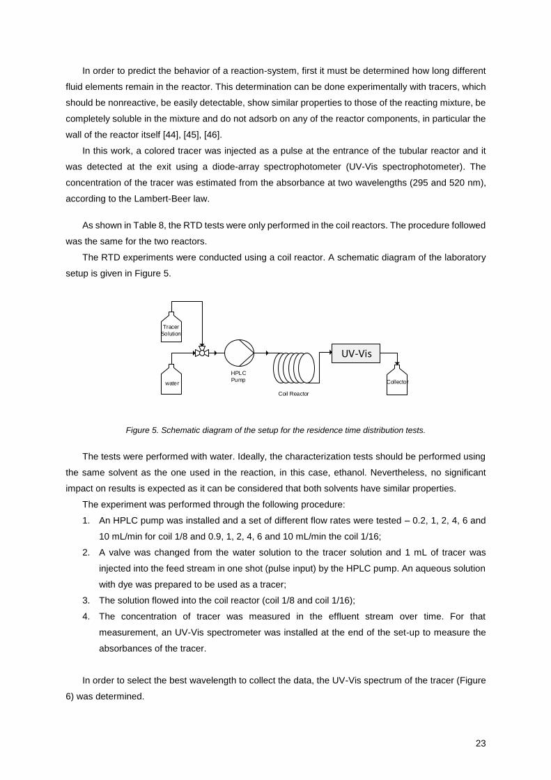
Citation preview
Characterization and scale-down of flow reactors for
applications at small-scale manufacturing
Margarida Marques da Silva Dias Coutinho
Thesis to obtain the Master of Science Degree in
Chemical Engineering
Supervisors:
Doutora Susana Isabel Massena do Nascimento
Professor Doutor Francisco Manuel da Silva Lemos
Examination Committee
Chairperson: Professor Doutor Carlos Manuel Faria de Barros Henriques
Supervisor: Doutora Susana Isabel Massena do Nascimento
Members of the Committee: Professor Doutor José Manuel Félix Madeira Lopes
November 2017


i
Acknowledgments
First of all I would like to thank Hovione FarmaCiência for the opportunity of this internship. This
experience was undoubtedly very rich not only in terms of technical knowledge, but also in terms of
personal experience. To meet many different people with different functions in the company made me
understand the importance of each one to ensure the good functioning and production of the company.
I want to express my gratitude to Ruth and Susana for the orientation during the internship, for the
time dedicated to me whenever I needed and for the knowledge shared. What I have learnt with them
will be a major benefit in the future.
I would like to thank professor Francisco Lemos, my academic supervisor for the precious help in
my thesis, for the patience and for the long hours dedicated to me. I also want to thank professor Amélia
Lemos, who although not being my supervisor, always received me so well and helped me when I
needed.
An infinite “thank you” to Mafalda for being my big company, support and friend during the
internship; to have shared with me all the moments during these months and to made this internship
much happier.
A word of appreciation to the chemists Rudi and Ana who helped me a lot during the internship and
always received me so well. In addition, to Rudi for the laboratory tests which data I used in the
development of this thesis.
Last but not least, I would like to thank my family for all the support and love. For always listening
to my problems and giving their opinion that I truly appreciate.

ii
iii
Resumo
A produção em contínuo tem vindo a ganhar destaque na indústria farmacêutica pela excelente
transferência de calor e massa que oferecem, que permite a possibilidade de intensificar os processos
usando novas gamas de operação que resultam num aumento da conversão e da qualidade do produto,
assegurando também a sua homogeneidade. O aumento da segurança e a redução de resíduos típicos
da indústria farmacêutica são também fatores fundamentais para a aplicação desta tecnologia.
O objetivo desta tese é caracterizar reatores contínuos e desenvolver uma metodologia de
scale-up/scale-down de processos químicos em contínuo. Para concretizar este objetivo, os reatores
foram caracterizados relativamente ao fluxo, com testes de distribuição de tempos de residência e à
transferência de calor. Para descrever as distribuições de tempos de residência obtidas foram usados
o modelo de uma bateria de reatores, o modelo de duas baterias em paralelo e o modelo da dispersão.
Em paralelo, a reação foi também caracterizada a partir dos dados da produção em batch e em reatores
contínuos de laboratório. Para o primeiro foi usado um modelo cinético baseado em balanços mássicos
e entálpicos e para os últimos, o modelo da segregação total e o modelo do pistão ideal.
A cinética da reação obtida com os dados em batch e em contínuo foi comparada, detetando-se
algumas diferenças que não eram expectáveis. Foram identificadas possíveis razões para estas
diferenças e foi proposta uma metodologia de scale-up e scale-down de reatores contínuos baseada
num abordagem de modelação.
Palavras-chave: reatores contínuos, scale-up/down, distribuição de tempos de residência,
transferência de calor, modelação, cinética química.

iv
v
Abstract
Continuous manufacturing is gaining increased attention in the pharmaceutical production due to
the excellent mixing and heat transfer offered that leads to the possibility of intensifying the process
using a range of new operating conditions that result in the increase of conversion and the quality of the
product, as well as ensuring a higher uniformity. Additionally, among the major advantages of continuous
manufacturing are the enhanced safety and reduction of waste which is crucial in the pharmaceutical
industry.
The scope of this thesis is to characterize flow reactors and develop a scale-up and scale-down
methodology for continuous reactors. In order to achieve this goal, a characterization of different
reactors and of the reaction itself was done. To study the dynamics of the reactors, residence time
distribution and heat transfer tests were performed in continuous laboratory reactors. In order to describe
the residence time distributions obtained, the model of tanks in series, the model of two batteries in
parallel and the dispersion model were applied. In parallel, the reaction kinetics was studied in the batch
reactor using a kinetic model based in the mass and energy balances and in continuous laboratory
reactors using the segregation model and the ideal PFR model.
The apparent kinetics of the same reaction performed in batch production mode and in the
continuous reactors was compared and some unexpected differences were found. Possible reasons for
this difference were identified and a scale-up/scale-down methodology procedures is purposed based
on a modelling approach.
Key-words: continuous reactors, scale-up/down, residence time distributions, heat transfer,
modeling, chemical kinetics.

vi
vii
List of Contents
Acknowledgments .....................................................................................................................................i
Resumo ................................................................................................................................................... iii
Abstract.....................................................................................................................................................v
List of Contents ....................................................................................................................................... vii
List of Figures .......................................................................................................................................... ix
List of Tables ........................................................................................................................................... xi
List of Schemes ..................................................................................................................................... xiii
1. Introduction ....................................................................................................................................... 1
1.1. Objectives and Motivation ....................................................................................................... 1
1.2. Thesis Layout .......................................................................................................................... 2
2. Literature Review ............................................................................................................................. 3
2.1. Batch vs. continuous ............................................................................................................... 3
2.2. Types of continuous reactors .................................................................................................. 5
2.2.1. Tubular Reactors ............................................................................................................. 5
2.2.2. Micro-reactors .................................................................................................................. 8
2.3. Scale-Up Strategies ............................................................................................................... 13
3. Experimental Part ........................................................................................................................... 19
3.1. Chemical Reaction ................................................................................................................ 19
3.2. Reactors studied .................................................................................................................... 20
3.3. Work Methodology ................................................................................................................. 21
3.4. Experimental Characterization of Continuous Reactors ....................................................... 22
3.4.1. Residence Time Distribution Tests ................................................................................ 22
3.4.2. Heat Transfer Tests ....................................................................................................... 24
3.4.3. Kinetic tests ................................................................................................................... 25
3.5. Mathematical Tools ............................................................................................................... 27
4. Experimental Results and Discussion ............................................................................................ 28
4.1. Residence Time Distributions ................................................................................................ 28
4.2. Heat Transfer ......................................................................................................................... 33
5. Models Results and Discussion ..................................................................................................... 35
5.1. Batch Reactor ........................................................................................................................ 35
5.2. Continuous Reactors ............................................................................................................. 38
5.2.1. Models for the Residence Time Distributions ................................................................ 38
5.2.2. Heat Transfer Models .................................................................................................... 58
5.2.3. Reaction Characterization Models................................................................................. 64
5.3. Conclusions ........................................................................................................................... 69
6. Methodology for Scale-up and Scale-down of continuous reactors ............................................... 71
7. Conclusions and Future Work ........................................................................................................ 74
8. References ..................................................................................................................................... 75
Supplementary information.................................................................................................................... 78

viii
Appendix A. Deductions of the Scaling factors: ............................................................................. 78
Appendix B. Experimental Residence Time Distributions for reactor coil 1/8 (295 nm) ................ 80
Appendix C. Experimental Residence Time Distributions for reactor coil 1/16 (295 nm) .............. 81
Appendix D. RTD for the Model of Tanks in Series for reactor coil 1/8 (295 nm) .......................... 82
Appendix E. RTD for the Model of Tanks in Series for reactor coil 1/16 (295 nm) ........................ 83
Appendix F. RTD for the Model of Two Batteries in Parallel for reactor coil 1/8 (295 nm) ............ 84
Appendix G. RTD for the Model of Two Batteries in Parallel for reactor coil 1/16 (295 nm) ......... 85
Appendix H. RTD for the Dispersion Model for reactor coil 1/8 (295 nm) ...................................... 86
Appendix I. RTD for the Dispersion Model for reactor coil 1/16 (295 nm) ..................................... 87
Appendix J. Deductions of equations present in Chapter 5 ........................................................... 88
ix
List of Figures
Figure 1. Types of reactors and the respective supplier. ........................................................................ 5
Figure 2. Illustration of the reactors from Cambridge Reactor Design [19]. ............................................ 7
Figure 3. Illustration of the reactor from Parr Instrument Company [22]. ................................................ 8
Figure 4. Corning micro-reactors. .......................................................................................................... 12
Figure 5. Schematic diagram of the setup for the residence time distribution tests.............................. 23
Figure 6. UV-Vis spectra of the tracer solution...................................................................................... 24
Figure 7. Schematic diagram of the setup for the heat transfer tests. .................................................. 24
Figure 8. Schematic diagram of the setup for kinetic tests in the reactor coil 1/16. .............................. 25
Figure 9. Schematic diagram of the setup for kinetic tests in the reactor MicR. ................................... 26
Figure 10. Experimental Residence Time Distribution for reactor coil 1/8 and coil 1/16 at the wavelength
of 520 nm. The green points represent the data for coil 1/8 and the red points for coil 1/16. A=0.2 mL/min
(coil 1/8); B= 0.9 mL/min (coil 1/16); C=1 mL/min; D=2 mL/min; E=4 mL/min; F=6 mL/min; G=10 mL/min.
............................................................................................................................................................... 30
Figure 11. Residence Time Distribution for all the flow rates for reactor coil 1/8. ................................. 31
Figure 12. Residence Time Distribution for all the flow rates for reactor coil 1/16. ............................... 31
Figure 13. The blue points represent the experimental residence time for each flow rate for coil 1/8 and
the orange line represents the residence times calculated by the internal volume............................... 32
Figure 14. The blue points represent the experimental residence time for each flow rate for coil 1/16 and
the orange line represents the residence times calculated by the internal volume............................... 32
Figure 15. Exit temperature of the reactor during the experiment for a flow rate of 2 mL/min. ............. 34
Figure 16. Exit temperature of the reactor during the experiment for a flow rate of 4 mL/min. ............. 34
Figure 17. Temperature difference between the experimental temperature and the temperature
calculated by the model for the production in batch mode. ................................................................... 37
Figure 18. Representation of the Model of Tanks in Series. ................................................................. 38
Figure 19. Influence of the Flow Rate in the RTD for the Model of Tanks in Series for reactor coil 1/8 at
the wavelength of 520 nm. The blue points represent the experimental data and the orange line is the
model of tanks in series. A=0.2 mL/min; B=1 mL/min; C=2 mL/min; D=4 mL/min; E=6 mL/min; F=10
mL/min. .................................................................................................................................................. 40
Figure 20. Influence of the Flow Rate in the RTD for the Tanks in Series Model for reactor coil 1/16 at
the wavelength of 520 nm. The blue points represent the experimental data and the orange line is the
model of tanks in series. A=0.9 mL/min; B=1 mL/min; C=2 mL/min; D=4 mL/min; E=6 mL/min; F=10
mL/min. .................................................................................................................................................. 42
Figure 21. Representation of the Model of two batteries in parallel. ..................................................... 44
Figure 22. Illustration of the two concentric reactors (side and top view) ............................................. 44
Figure 23. Influence of the Flow Rate in the RTD for the Two Batteries in Parallel Model for reactor coil
1/8 at the wavelength of 520 nm. The blue points represent the experimental data and the orange line
is the model of two batteries in parallel. A=0.2 mL/min; B=1 mL/min; C=2 mL/min; D=4 mL/min; E=6
mL/min; F=10 mL/min. ........................................................................................................................... 45
x
Figure 24. Influence of the Flow Rate in the RTD for the Two Batteries in Parallel Model for reactor coil
1/16 at the wavelength of 520 nm. The blue points represent the experimental data and the orange line
is the model of two batteries in parallel. A=0.9 mL/min; B=1 mL/min; C=2 mL/min; D=4 mL/min; E=6
mL/min; F=10 mL/min. ........................................................................................................................... 47
Figure 25. Global adjustment for the Model of the Two Batteries in Parallel for reactor coil 1/16 at the
wavelength of 520 nm. The blue points represent the experimental data and the orange line is the model
of two batteries in parallel. A=0.9 mL/min; B=1 mL/min; C=2 mL/min; D=4 mL/min; E=6 mL/min; F=10
mL/min. .................................................................................................................................................. 51
Figure 26. Representation of the dispersion model [48]. ...................................................................... 52
Figure 27. Dispersion in a tubular reactor [46]. ..................................................................................... 52
Figure 28. Representation of the two boundary conditions: closed and open vessel [48]. ................... 53
Figure 29. Influence of the Flow Rate in the RTD for the Dispersion Model for reactor coil 1/8 at the
wavelength of 520 nm. The blue points represent the experimental data and the orange line is the
dispersion model. A=0.2 mL/min; B=1 mL/min; C=2 mL/min; D=4 mL/min; E=6 mL/min; F=10 mL/min.
............................................................................................................................................................... 55
Figure 30. Influence of the Flow Rate in the RTD for the Dispersion Model for reactor coil 1/16 at the
wavelength of 520 nm. The blue points represent the experimental data and the orange line is the
dispersion model. A=0.9 mL/min; B=1 mL/min; C=2 mL/min; D=4 mL/min; E=6 mL/min; F=10 mL/min.
............................................................................................................................................................... 57
Figure 31. Heat Transfer Model for reactor coil 1/8 at the flow rate of 2 mL/min. ................................. 59
Figure 32. Heat Transfer Model for reactor coil 1/8 at the flow rate of 4 mL/min. ................................. 60
Figure 33. Heat Transfer Model for reactor coil 1/8 considering the dynamics of the sensor (flow rate of
2 mL/min). .............................................................................................................................................. 61
Figure 34. Heat Transfer Model for reactor coil 1/8 considering the dynamics of the sensor (flow rate of
4 mL/min). .............................................................................................................................................. 61
Figure 35. Heat Transfer Model for reactor coil 1/8 considering the dynamics of the sensor and heat
losses (flow rate of 2 mL/min)................................................................................................................ 63
Figure 36. Heat Transfer Model for reactor coil 1/8 considering dynamics of the sensor and heat losses
(flow rate of 4 mL/min). .......................................................................................................................... 63
Figure 37. Segregation model for a PFR [46]........................................................................................ 65
Figure 38. Experimental and calculated conversion by the Segregation Model for reactor coil 1/16. .. 66
Figure 39. Theoretical RTD for an Ideal Plug Flow Reactor. ................................................................ 67
Figure 40. Experimental and calculated conversion by the Ideal PFR Model for reactor coil 1/16. ...... 67
Figure 41. Experimental and calculated conversion by the Ideal PFR Model for reactor MicR. ........... 68
xi
List of Tables
Table 1. Characteristics of the Cambridge Reactor Design reactors [19]–[21]. ...................................... 7
Table 2. Characteristics of the Parr Instrument Company reactors [22]. ................................................ 8
Table 3. Characteristics of Chemtrix reactors [28]–[32]. ....................................................................... 10
Table 4. Characteristics of Corning reactors [33]–[36]. ......................................................................... 11
Table 5. Normalized parameters in this work. ....................................................................................... 19
Table 6. Feasibility assessment for transfer of a process from batch to continuous, applied to the case
study. ..................................................................................................................................................... 19
Table 7. Reactors technical data and operating ranges. ....................................................................... 20
Table 8. Characterization tests performed in each continuous reactor. ................................................ 22
Table 9. Summary of the reaction conditions and results of the kinetic tests in reactor coil 1/16. ........ 26
Table 10. Summary of the reaction conditions and results of the kinetic tests in continuous MicR...... 27
Table 11. Residence time for each flow rate for coil 1/8 and coil 1/16. ................................................. 32
Table 12. Parameters for the calculation of UA..................................................................................... 33
Table 13. Kinetic parameters obtained from the production in batch mode. ......................................... 37
Table 14. Models applied to each continuous reactor. .......................................................................... 38
Table 15. Main parameters of the model of tanks in series for reactor coil 1/8. ................................... 41
Table 16. Main parameters of the model of tanks in series for reactor coil 1/16. ................................. 43
Table 17. Main parameters of the model of two batteries in parallel for reactor coil 1/8. ..................... 46
Table 18. Main parameters of the model of two batteries in parallel for reactor coil 1/16. ................... 48
Table 19. Summary of the global adjustment of the two batteries in parallel mode for reactor coil 1/16.
............................................................................................................................................................... 50
Table 20. Summary of the parameters for the Dispersion Model for reactor coil 1/8. .......................... 55
Table 21. Summary of the parameters for the Dispersion Model for reactor coil 1/16. ........................ 57
Table 22. Summary of the dimensionless numbers analyzed in this chapter. ...................................... 58
Table 23. Parameters used in the Heat Transfer Models ..................................................................... 58
Table 24. Parameters adjusted for optimization of the Heat Transfer Model considering only dynamics
of the sensor. ......................................................................................................................................... 62
Table 25. Parameters adjusted for optimization of the Heat Transfer Model considering dynamics of the
sensor and heat losses. ......................................................................................................................... 63
Table 26. Kinetic parameters obtained from the Segregation Model for reactor coil 1/16. ................... 66
Table 27. Kinetic parameters obtained from the Ideal PFR Model for reactor coil 1/16. ...................... 68
Table 28. Kinetic parameters obtained from the Ideal PFR Model for reactor MicR............................. 68
Table 29. Summary of the kinetic parameters obtained from batch and continuous mode. ................. 69
Table 30. Temperatures assumed as real and estimated by the Segregation Model and Ideal PFR Model
for reactor coil 1/16 and MicR. .............................................................................................................. 70
Table 31. Relationship between a chemical reaction and the reactor. ................................................. 71

xii

xiii
List of Schemes Scheme 1. Thesis work methodology ................................................................................................... 22
Scheme 2. Proposed methodology for Scale-Up of continuous reactors. ............................................ 73

xiv
1
1. Introduction
1.1. Objectives and Motivation
Pharmaceutical manufacturing operates typically in batch mode. The versatility and flexibility
offered by batch processes constitute significant advantages that justify the selection of this operation
mode. However, in the recent years, continuous manufacturing is increasingly addressed in the
pharmaceutical industry as a way to modify traditional batch processes, reflecting the endorsement
being made by Regulatory Agencies, mainly Food and Drug Administration (FDA), and the press
releases from big pharma and biotech companies announcing big investments in the field. If improved
mixing and heat transfer can be achieved, the process can be intensified and new operating conditions
can be used, increasing conversion and the quality of the product, as well as ensuring a higher uniformity
and throughput. Additionally, continuous flow processing might also allow accessing a range of reactions
conditions that would otherwise not be accessible, such as processes which are a combination of high
temperature, high pressure and short reaction times, for instance.
One of the major advantages of continuous manufacturing is the enhanced safety not only because
of the reduced inventory of raw materials and solvents, but also because the hold times between
operations can be eliminated, leading to no unstable or hazardous intermediate accumulation. The real
time control and higher automation make sure all the parameters are within the range and the product
is being manufactured as intended, thus improving the quality of the product [1], [2].
Hovione is building capabilities to use continuous manufacturing for API synthesis and drug product
to use it as a differentiator element. Moving a process from batch to a continuous processing mode
requires a profound knowledge on the reactor performance, matching its characteristics to the reaction
kinetics.
The scope of this thesis is to characterize two main types of flow reactors for small-scale
manufacturing of Active Pharmaceutical Ingredients (APIs) in order to purpose a scale-up/scale-down
methodology to make scale-up and scale-down operations easier and more reliable. Every time a
specific product is to be manufactured in the production scale, preliminary studies have to be carried
out in the laboratory to allow the correct design of the manufacturing procedure and to select the most
suitable reactors for the necessary reactions. However, in some cases, the conditions that work well in
a laboratory scale do not work so well in the production scale. Laboratory equipment has a very small
size, which leads to an almost perfect mixing and an excellent heat and mass transfer, due to the larger
area/volume ratio. On the other hand, when the reaction is carried out in a production scale reactor, due
to its larger size, heat and mass transfer become more heterogeneous and it is more difficult to ensure
that all the reaction mixture is well mixed. For this reason, the conditions used in the production scale
have to be adapted.
In order to achieve the goal of making a correct scale-up and/or scale-down of continuous reactors,
this work focused on a contribution for the characterization of different reactors and of the reaction itself.
To study the dynamics of the reactors, flow characterization tests were performed in two different
continuous laboratory reactors, and heat transfer tests in one them. For the flow characterization, RTD
2
tests were carried out and the data was fitted applying the model of tanks in series, the model of two
batteries in parallel and the dispersion model. The reaction kinetics in the batch reactor and in two
different continuous laboratory reactors was also studied, and the segregation model and the ideal PFR
models were applied.
The apparent kinetics of the same reaction, performed in batch manufacturing mode in the
production scale was compared to the results obtained for the continuous laboratory reactors and
possible reasons for the differences observed were addressed.
A set of recommendations was established to provide a methodology for scale-up/scale-down
procedures.
1.2. Thesis Layout
A brief explanation about the structure of this thesis will be given in this section.
Chapter 2 provides an overview of the available literature on the most relevant concepts, including
the issues involved in the transition of the pharmaceutical production from batch to continuous
manufacture, the characteristics of commercial continuous reactors applied to pharmaceutical industries
and methodologies for scale-up/scale-down continuous processes. In chapter 3, an explanation of the
experimental part is given, including a description of the reaction and materials used as a case study,
as well as the experimental tests performed. Chapter 4 includes the results and discussion of the
experimental results obtained. Chapter 5 presents the results and explains the models applied to the
data presented in previous chapter. In Chapter 6 a methodology for scaling-up/scaling-down continuous
processes is presented. An overall discussion of the results and final remarks describing the impact of
the developed work and addressing suggestions for future work is presented in Chapter 7.
3
2. Literature Review
2.1. Batch vs. continuous
Batch manufacturing is a long process which uses large-scale equipment and is the preferred mode
of operation for the production of Active Pharmaceutical Ingredients (APIs). However, in the recent
years, continuous manufacturing has been encouraged to be used as a more efficient process, to create
a more robust and flexible method capable of manufacturing high-quality APIs [3], [4].
Concerning the advantages of batch manufacturing, flexibility and a readily reconfigurable set of
multipurpose unit operations are often thought of. A large number of products can be manufactured in
a single plant with multiple stirred tank reactors [1], [5]. High conversions can be achieved by keeping
the reactants for a long time in the reactor. Very slow transformations that cannot be accelerated by
increased heating and cooling are often best performed in batch reactors [6].
Nevertheless, the production in batch mode takes a longer time due to the existence of several
reaction steps as well as isolation and purification work-up operations between each reaction step [7].
Because of the hold times between steps, unstable species can be accumulated, making it a less safe
process. Another disadvantage of the batch manufacturing is the high technical challenges of scaling-up
batch operations from the laboratory to pilot scale and to manufacturing scale due to the difficulty in
maintaining mixing and heat transfer conditions along the production scales. Hence, the reaction
conditions can vary with location in the reactor leading to undesirable side products [1], [5].
The expectation is that more companies will invest in continuous manufacturing technologies with
the aim of gaining a significant competitive advantage. As the pharmaceutical manufacturing industry
progresses, higher-quality drugs will be produced faster and more cost effectively, benefiting patients
around the world [8]. Current estimates suggest a general increase in industrial continuous
manufacturing applications from 5% to 30% over the next few years [9].
In continuous manufacturing, due to the efficient mixing and excellent heat exchange of the reactors,
extreme conditions might be used in a safe way, leading to a reduction of raw materials and solvents
usage and, consequently, less costs. New reaction conditions can be applied, and processes that are
simply not viable in traditional batch mode operations will be able to be exploited [10]. These new
patterns include a new range of substrates and operational conditions, such as higher concentrations,
temperatures and pressures that will hopefully increase conversion and the quality of the product. This
is called process intensification, which is a chemical engineering development that leads to a smaller,
cleaner, and more efficient process [11].
Due to the small size of the flow equipment, a small amount of hazardous intermediates is formed
at any instant, what leads to an improvement of safety issues. Also, the better control of exothermic
reactions improve safety what constitutes a major advantage of continuous manufacturing [9], [12]. The
small amount of hazardous intermediates also reduces the environmental footprint and helps to
minimize issues of waste and energy usage typical of a pharmaceutical industry [12].
4
A key advantage of flow reactor technology is the ability to accurately control and monitor reaction
parameters. It is of upmost importance to consistently manufacture a product that has a uniform
character and quality attributes within specific limits [2], [5], [13]. This is possible thanks to the high
automation and in-line control implicit in continuous technology.
The reaction temperature, pressure, concentration, flow rate and residence time are very important
operating parameters for maintaining reaction under control and ensure selective product formation and
preserve intermediates degradation. Furthermore, the total flow of the streams ensures proper
residence time and the ratio between the flows of each stream ensures proper stoichiometry of the
reagents. The control of the flow rate and therefore of the residence time is crucial for handling highly
reactive intermediates [1], [10], [14].
In a continuous reactor, mixing is rapid and heat can be readily added or removed from the reactor,
which results in a higher yield [9] [10]. The high surface area also allows for an excellent control of
exothermic reactions. As well as increasing the rate of mixing, decreasing the reactor channel diameter
results in a high surface to volume ratio, what leads to a rapid dissipation of the heat generated during
the reaction [13].
Despite the innumerous advantages associated with continuous manufacturing mode enumerated
above, it needs to be noted that it is far from certain that flow technology will solve the current problems
in the pharmaceutical sector [14]. The current inventory of available batch manufacturing facilities is one
of the biggest barriers for the implementation of continuous manufacturing units. It constitutes a high
capital investment to change the facilities to continuous mode [2], [5]. Another barrier to the
implementation of continuous manufacturing is the successes of the batch technology. In order to
achieve a successful transformation, the mind-set has to change [9], [15].
Although the transition to continuous manufacturing has been highly successful in some cases,
resulting in a transformative change through market growth and expansion, the initial implementation is
slow due to the technical challenges and firm mind-sets fixed in the old technology [15].
5
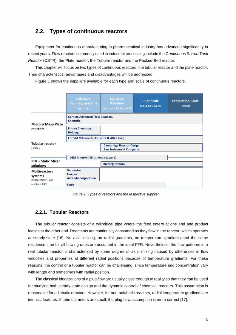
2.2. Types of continuous reactors
Equipment for continuous manufacturing in pharmaceutical industry has advanced significantly in
recent years. Flow reactors commonly used in industrial processing include the Continuous Stirred Tank
Reactor (CSTR), the Plate reactor, the Tubular reactor and the Packed-Bed reactor.
This chapter will focus on two types of continuous reactors: the tubular reactor and the plate reactor.
Their characteristics, advantages and disadvantages will be addressed.
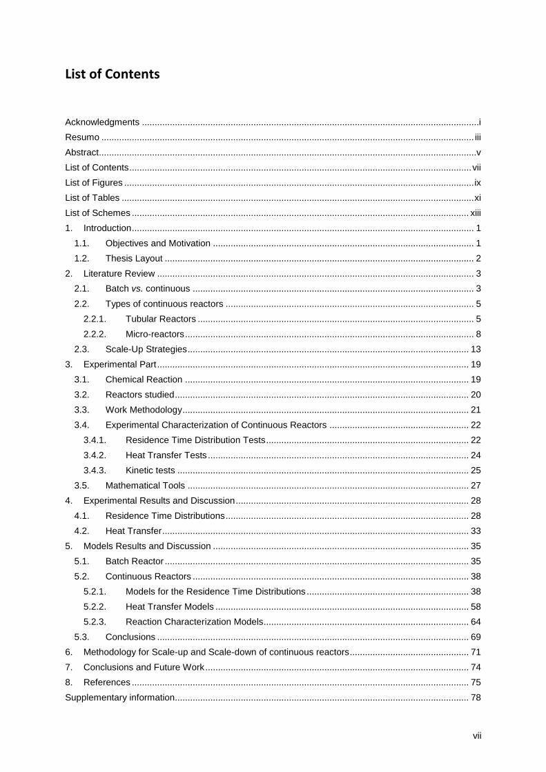
Figure 1 shows the suppliers available for each type and scale of continuous reactors.
2.2.1. Tubular Reactors
The tubular reactor consists of a cylindrical pipe where the feed enters at one end and product
leaves at the other end. Reactants are continually consumed as they flow in the reactor, which operates
at steady-state [16]. No axial mixing, no radial gradients, no temperature gradients and the same
residence time for all flowing rates are assumed in the ideal PFR. Nevertheless, the flow patterns in a
real tubular reactor is characterized by some degree of axial mixing caused by differences in flow
velocities and properties at different radial positions because of temperature gradients. For these
reasons, the control of a tubular reactor can be challenging, since temperature and concentration vary
with length and sometimes with radial position.
The classical idealizations of a plug flow are usually close enough to reality so that they can be used
for studying both steady-state design and the dynamic control of chemical reactors. This assumption is
reasonable for adiabatic reactors. However, for non-adiabatic reactors, radial temperature gradients are
intrinsic features. If tube diameters are small, the plug flow assumption is more correct [17].
Lab scale Capillary systems
(μg to mg)
Lab scale KiloFlow
(mg to Kg’s, 1-2 Kg 1 week)
Pilot Scale(10-50 Kg, 1 week)
Production Scale(>50 Kg)
Micro & Meso Plate reactors
Corning Advanced Flow ReactorsChemtrix
Tubular reactor(PFR)
Agitated Cell Reactor
Spinning Disc reactor
Multireactors systems (microreactor + coil
reactor + PBR)
Cambridge Reactor DesignParr Instrument Company
VapourtecUniqsisAccendo Corporation
FlowID
AM Technology
Future Chemistry Holding
Syrris
DSM Innosyn (3D printed reactors)
Oscillatory Baffled Reactor Nitech Solutions
PFR + Static Mixer solutions
Fluitec|FlowLink
Packed Bed Reactor(PBR)
ThalesNanoNippon Kodoshi Corporation
Iberfluid|PID
Parr Instrument Company
Ehrfeld Mikrotechnik (Lonza & Alfa Laval)
Figure 1. Types of reactors and the respective supplier.
6
The diameter of tubular reactor can range from a few millimeters to several meters. The choice of
diameter is based on construction cost, pumping cost, the desired residence time, and heat transfer
needs. Typically, long small diameter tubes are used with high reaction rates and larger diameter tubes
are used with slow reaction rates.
When the reactor operates adiabatically there is no external heat transfer along the reactor. Whether
the reaction generates or consumes heat, the temperature of the material flowing in the reactor
increases or decreases, respectively [17].
In tubular reactors, the heat transfer and temperature control are achieved by the use of heat
exchangers which can be concentric tubes or shell and tube. Heat exchangers increase surface area to
volume ratio leading to an improvement of heat transfer rates. They might be used to adjust the
temperature of raw materials and to control the temperature in the mixing zone [1].
Tubular reactors have a wide variety of applications in either gas or liquid phase systems and for
both small and industrial production [16]. They denote a good balance between cost, heat and mass
transfer efficiency, and easy mode of operation [1].
Summarizing, some advantages and disadvantages of this type of continuous reactors are
addressed as follows:
Advantages ([16], [18]): Disadvantages ([16], [18]):
Easily maintained because of the non-
existing moving parts;
High conversion rate per reactor volume;
Mechanically simple;
Constant product quality;
Adequate for studying rapid reactions;
Efficient use of reactor volume;
Good for large capacity processes;
Low pressure drops;
High conversion per unit volume;
Low operating cost;
Good heat transfer;
Easy to clean.
Reactor temperature difficult to control;
Hot spots may occur within reactor when
used for exothermic reactions, leading to
undesired thermal gradients;
Difficult to control due to temperature and
composition variations;
Shutdown and cleaning may be
expensive.
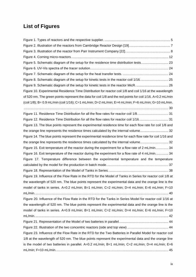
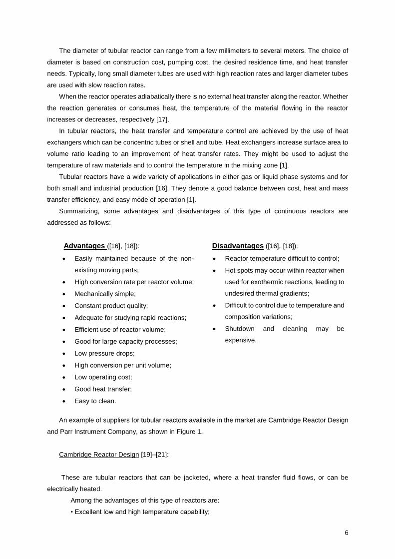
An example of suppliers for tubular reactors available in the market are Cambridge Reactor Design
and Parr Instrument Company, as shown in Figure 1.
Cambridge Reactor Design [19]–[21]:
These are tubular reactors that can be jacketed, where a heat transfer fluid flows, or can be
electrically heated.
Among the advantages of this type of reactors are:
• Excellent low and high temperature capability;
7
• Excellent pressure capability with optional pressure control unit;
• Modular design offering variable residence times;
• Material: Stainless steel, Hastelloy or PEEK coils;
• Can be empty of a packed column;
• Very low cost.
The main characteristics and operational conditions are summarized in Table 1 and an example
of the reactors are illustrated in Figure 2.
Table 1. Characteristics of the Cambridge Reactor Design reactors [19]–[21].
Characteristics
Salamander Jacketed
Reactor with Capillary
Tubing
Salamander Jacketed
Reactor with Static Mixers
Temperature Range (ºC) -80 – 300 -80 – 200
Max. Pressure (bar) 200 25
General Material 316 Stainless Steel/ Hastelloy
C276 alloy
316 Stainless Steel/ Hastelloy
C276 alloy
Diameter (mm) 75 315
Length (mm) 500 500
Shell Side Volume (L) 1 2
Insulation None/Silicone Sponge None/Silicone Sponge
Diameter (inches; mm) 1/16’’; 1.6 6
Length (m) 18 300
Tude Side Total number of tubes max. 5 12
Max. Operating Volume
(mL) 18 100
Min. Operating Volume
(mL) 0,1 8,5
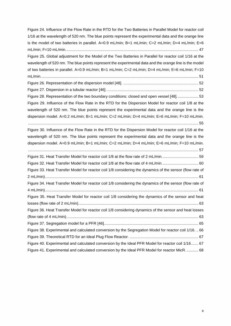
Parr Instrument Company [22]:
These are tubular reactors which can be heated by an external furnace or be jacketed with a
circulating heat transfer fluid for heating or cooling. They may be empty when performing homogeneous
reactions, or packed with catalyst.
Figure 2. Illustration of the reactors from Cambridge Reactor Design [19].
8
The main characteristics and operational conditions are summarized in Table 2 and Figure 3
represents an illustration of the reactor.
Table 2. Characteristics of the Parr Instrument Company reactors [22].
Series 5400 Tubular Reactor System Specifications
Model Number 5401 5402 5403 5404
O.D. / I.D. (mm) 9.5 / 7.0 13 / 9.4 48 / 25 51 / 38
Heated Length (cm) 15.2, 30.5, 61 30.5, 61, 91.4
Max. Pressure (bar) 207 345 207
Max. Temperature (ºC) 550 550 350
Figure 3. Illustration of the reactor from Parr Instrument Company [22].
2.2.2. Micro-reactors
The microplate reactor (lab scale) or meso-scale plate reactor (pilot and production scale) are based
on a modified plate heat exchanger design. It consists of reactor plates, inside which the reactants mix
and react, and utility plates, inside which a cooling or heating fluid flows. There is one utility plate on top
and one below each reactor plate.
Plate reactors are identified as a choice of excellence when compared with batch reactors in highly
exothermic and very fast reactions as they allow 100 times better heat and mass transfer than batch
reactors.
Micro-reactors channel diameter ranges from 50 to 500 μm, channel length between 1 to 50 μm and
the surface-to-volume ratio is between 100 to 50 000 m2/m3. They are usually made of materials as
silicon, quartz, glass, metals and polymers. Glass reactors are the most commonly used due to their
higher chemical compatibility with the reagents and solvents, but silicon, or a mixture of silicon and glass
reactors are also common [13].
Flow micro-reactor systems can be used for production on a relatively large scale because although
the reactor volume is small, the total production over time is much superior than usually believed [23].
9
The micro-reactor is a modular reactor and each module can address one process step: feeds pre-
mixing, chemical reaction, thermal/chemical quench. The exceptional heat-exchange efficiency and
almost instantaneous mixing of micro-reactors, thereby maintaining a controlled temperature profile
along the reaction path, allows a significant decrease of secondary products through improved yield and
selectivity, avoids the formation of hot spots, temperature gradients and accumulation of heat,
constituting a safer technology.
Pressure drop is very important at high flow rates especially with viscous systems and low
temperatures. The mixing zone is often the plate section that consumes the larger pressure drop. A way
to considerably reduce the overall pressure drop is to enlarge mixer elements at higher flow rates [24],
[25].
In order to fulfill the requirements, the reactor has to be resistance to the reaction mixture, the wall
of the reactor has to be thermal conductive to avoid heat transfer problems, it has to be mechanically
resistant to the high pressures and temperatures, being easy to manufacture and have good material-
cost relationship [26]. In addition to liquid phase reactions, micro reactor technology is also highly suited
to reactions involving gases.
The advantages of micro-reactors over the tubular reactors are related to the special structures such
as mixing geometries that offer highly improved mixing performance and enhanced heat transfer
promoting easier temperature control. A disadvantage of micro-reactors is that is significantly more
expensive than tubular reactors [1].
In order to understand the number of reactions that could fit into the characteristic mixing and
residence time of microreactors, Lonza Group classified the reactions based on their physicochemical
properties, both in terms of reaction kinetics and phases. The reaction kinetics were categorized in three
main classes [24], [27]:
Type A reactions:
o Very fast reactions (< 1 s);
o Mainly controlled by the mixing process;
o In general, the reaction yield is increased by rapid mixing and enhanced heat exchange
performances when using a micro-reactor.
Type B reactions:
o Rapid reactions (10 s to 20 min);
o Predominantly controlled by the kinetic;
o The yield is increased by a precise control of the residence time and temperature.
Type C reactions:
o Slow reactions (> 20 min);
o Often operated batch wise;
o A large heat accumulation is observed, thus the use of a continuous process will enhance
safety with the prerequisite that process intensification has taken place when using an
alternative technology.
10
For micro-plate reactors, the example of the suppliers available in the market presented in this
subchapter are Chemtrix and Corning Advanced Flow Reactors.
Chemtrix [28]–[32]:
The main characteristics and operational conditions are summarized in Table 3.
Table 3. Characteristics of Chemtrix reactors [28]–[32].
Reactor Scale Operational conditions
Labtrix
Laboratory
Temperature: -20 to 195 ºC
Pressure: up to 25 bar
Residence Time: 1.2 s to 97.5 min
Production Capacity: 0.1 to 100 μL/min
KiloFlow
Temperature: -20 to 150 ºC
Pressure: up to 20 bar
Production Capacity: 0.2 to 100 mL/min (up to
6 kg/h)
Protix
Temperature: -30 to 200 ºC
Pressure: up to 25 bar
Production Capacity: 0.2 to 20 mL/min
Plantrix
Pilot Plant
Temperature: -30 to 200 ºC
Pressure: up to 25 bar
Production Capacity: 1 to 36 L/h
Production Scale
Temperature: -30 to 200 ºC
Pressure: up to 25 bar
Production capacity: 5 to 400 L/h
11
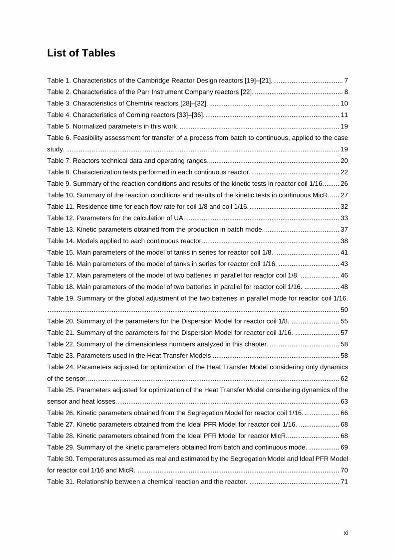
Corning Advanced Flow Reactors [33]–[36]:
The main characteristics and operational conditions are summarized in Table 4.
Table 4. Characteristics of Corning reactors [33]–[36].
Scale Picture Flow Rate Single plate volume Temperature Pressure Materials
Low-Flow
2-10 mL/min 0.45 mL -10 – 200ºC ≤18 bar Glass PFA perfluoroelastomer
G1
30 – 200 mL/min 8-11 mL -60 – 200ºC ≤18 bar Glass PFA perfluoroelastomer
G3
400 – 2000 mL/min
55-65 mL ~1000 ton/year
-60 – 200ºC ≤18 bar Glass PFA perfluoroelastomer
G4
1000 – 8000 mL/min
200-260 mL ~2200 ton/year ~300 kg/h
-60 – 200ºC ≤18 bar
Silicon carbide PFA Perfluoroelastomer
12
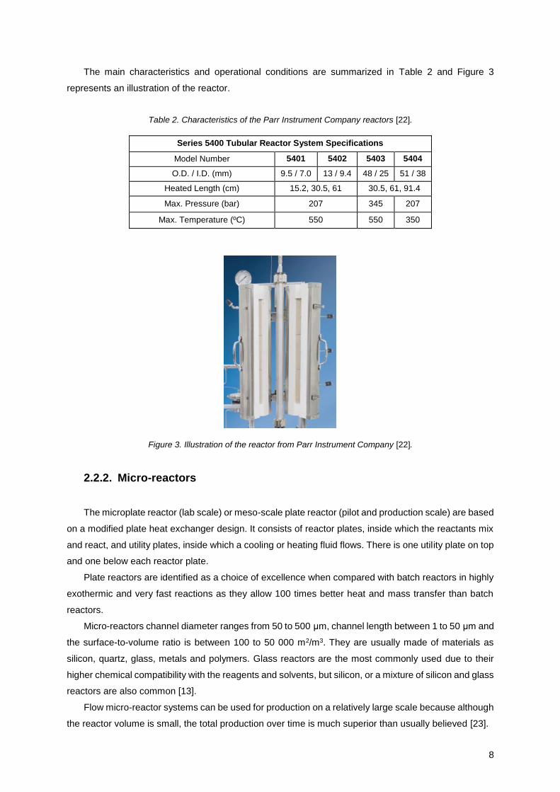
These micro-reactors offer excellent mixing and heat exchange due to the patented HEART design,
constituting a major advantage and is what differentiate them from the other micro-reactors. They all are
highly flexible and multipurpose, offer a seamless scale-up and have high chemical durability. In Figure
4 two examples of the Corning micro-reactors are presented, where it can be seen the complexity of
these reactors.
Figure 4. Corning micro-reactors.
13
2.3. Scale-Up Strategies
It is possible to divide the traditional scale-up procedures in three different approaches [37]:
1. Physical approach:
This approach uses dimensionless numbers and dimensionless variables which have to be kept
constant at both scales.
2. Experimental or empirical approach:
In this approach the knowledge and the experience of the process is used to do the scale-up. Two
different methods can be followed: trial and error, in which experimental process data are used for the
construction of empirical relations, and the use of rules of thumb.
3. Fundamental approach:
This approach involves proper modeling for the description of the process behavior (model-based
scale-up). Mathematical models of chemical processes have great potential in engineering applications
as they can be used as a tool for prediction, control, design and optimization of processes. The
mathematical model may be a simple or a complex one within available data, knowledge, ideas and
objectives. One can choose within transport phenomena models, population balance models, empirical
models or combinations of them. These models are supported on the availability of good enough models
that enable the analysis of process dynamics [38].
Moreover, it must be always remembered the fact that if a model gives a good description of reality,
it does not necessarily mean that the assumptions upon which it is based are true [38].
The laboratory reactor should not necessarily be similar to the idea we have of industrial one but
has to be designed in order to give the best information. In particular, fluid dynamics and transport
properties are to be accurately checked. Experiments should be carried out, if possible, in a sequential
way and should be followed by a mathematical modeling analysis in order to improve their quality and
to provide the first tools for scaling up [38].
One area of considerable importance to reaction engineering is kinetics and this is the area of
greatest uncertainty. We do not need to know the “true kinetics” but we must know for sure the relation
between what is derived from the laboratory experiments and what is used to design an industrial
reactor, side effects included [38].
This approach will be detailed in chapter 6 as it is the final goal of this work.
The physical approach involves three ways for the scale-up of tubular and micro-reactors:
1. Numbering-up, by adding identical reactors in parallel;
2. Scaling in series, by making the tube longer or adding several reactors in series;
3. Scale-out, by suitable dimension enlarging. For a tubular reactor either increasing the tube
diameter but keeping constant length or increase both tube diameter and length. For micro-plate
reactor by increasing the plate size.
In a continuous reactor, to increase the flow processed per hour, the volume of the reactor has to
increase as well. Mixing, heat transfer and residence time have to be maintained in the large scale to
achieve the same production, under the same conditions, as in the small scale. The design criterion for
14
continuous processes is the residence time that should not change with scale. For this reason, the
majority of scale-up of continuous processes occurs by increasing the total reactor volume and the flow
rate to maintain the residence time established during development and at smaller scale [1].
1. Numbering-up: identical reactors in parallel:
In the parallel numbering-up, the number of tubes is increased in direct proportion to the desired
increase in throughput providing that the feed distribution between the tubes is uniform. This means that
a single tube should represent the range of behaviors in a multitubular design and the distribution of
flow on the shell side ought to be uniform enough to guarantee in all the tubes the same heat transfer
coefficient [39].
This method has the advantages of keeping most of the relevant parameters constant, including a
constant pressure drop, hydrodynamics and heat transfer characteristics. It also avoids many scale-up
effects as little changes in reaction conditions are needed. However, there are significant challenges of
maintaining uniform fluid distribution to each reactor. Commercial processes would require a high
degree of automation to ensure proper flow at all times. This represents a significant challenge of this
way of scaling-up. An extra energy consumption is also associated with the control of the flow rate per
reactor and may lower the reactor flow rate operating window [40], [1], [41].
In micro-reactors, stacking reactors plates is often applied because sandwiching heating/cooling
plates between the reaction plates easily maintains heat transfer conditions [40]. Nonetheless, too many
reactors in parallel would lead to a complex and costly unit, with a lot of shut down and maintenance
costs. It is not expected to have more than 10-12 reactors in parallel, and for some cases up to 20 (when
the number of fluid to distribute is low).
In this scenario, the replication of the same geometries and flow rates for each unit provides the
higher overall process flow rates, and thus avoids any scale-up effects. The logistics, complexity and
capital investment of such systems may limit widespread implementation for high-volume products.
2. Scaling in series:
Scaling in series consists in keeping a constant tube diameter and increasing the tube length. To
ensure the same residence time, if the length is doubled, the flow rate have to be doubled too [39].
In the case of micro-reactors, this approach consists in adding several plates in series, keeping one
reactant at a high flow rate and adding the second stepwise in series. This aims at ensuring longer
channels in various segments and a consistent residence time when flow rates are increased. This
strategy has the advantage of requiring fluid distributors, which helps the operation to achieve the
required flow control and lower the costs. However, due to the impossibility of increasing flow rates
unlimitedly, this scale up method is limited, although a large range of flow rates from milliliters to several
hundred milliliters per minute is possible for specific reactors [1], [40].
In order to keep the residence time value, this would lead to high velocities, higher channel length
and a much higher pressure drop, which is a very limiting factor and the major problem of this scaling
15
method. In order to mitigate the pressure drop increase, the channel height can be increased provided
that heat transfer coefficient does not change significantly.
3. Increase the size of the tube/plate:
The last strategy is scale-up by selective dimension increasing.
In the case of micro-reactors, the channel/plate size is increased to achieve the desired production.
However, it is critical to preserve the advantages of fast mixing and excellent heat and mass transfer
inherent of micro-reactors [40].
In tubular reactors, to change reactor dimensions is a common strategy. However, changes in the
size of the reactor affect the quality of initial mixing, the dispersion characteristics of a system and the
increase of the tube diameter leads to the modification of the heat transfer coefficient. For this reason,
understanding the effects of flow and heat characteristics of the fluid is of high importance to the scale-
up process [41].
If there are some concerns on heat transfer, it may be advantageous to increase the tube diameter
in order to limit the pressure in the industrial plant. One way to do this is to scale with geometric similarity,
a common scale-up method for stirred-tanks reactors but less common for tubes. To achieve the desired
throughput, the diameter could be increased while keeping the same length-to-diameter ratio [39].
When the flow is laminar, using geometric similarity ensures the same pressure drop but for
turbulent flow the pressure drop will be higher. In the last case, to achieve the same pressure drop the
tube needs to be shorter and wider [39].
A seamless scale-up will be achieved, when moving from a small continuous reactor, to a larger
one, if you apply the same parameter as in the laboratory (temperature, residence time, concentration,
stoichiometric ratio), you will get the same result in production (conversion, yield, impurity profile).
The industrial unit will be made based on:
The operating data obtained in laboratory:
Total flow rate
Reaction temperature
Concentration of final product
Residence time
Total pressure drop
The desired annual production of the industrial unit:
Quantity of product
Number of hours worked per year
Different suppliers have different approaches of scale-up: increase the lateral dimensions of the
channel of the micro-reactor for the double while maintaining a sufficient large surface to volume ratio
(S/V); increase the volume of the plate reactor by incorporating communicating channels, which provides
a good internal distribution. This constitutes a way of increasing the volume with no significant changes
in the flow hydrodynamics, mass and heat transfer coefficients. This supplier achieves scale-up from
16
the pilot plant to the production plant by combining the three ways of scale-up (increase the size plate
by a certain factor, as well as adding some reactors in series and some in parallel).
The same supplier states that by increasing the height of the plate by a factor of 5 decreases the
S/V ratio by the same factor. Consequently, the surface heat transfer coefficient has to be multiplied by
5. In the production scale the material of construction is changed by another one with a 100 times higher
thermal conductivity leading to a huge increase of the heat transfer coefficient.
In a continuous reactor, to increase the flow processed per hour we need to increase the volume
of the reactor as well. To achieve the same result, mixing and heat transfer must be kept at the same
value and RTD at a similar level.
The main parameters being scaled-up is the heat removal capacity, which has to be kept constant
among different sizes. Heat transfer can be the key concern in reactor scale-up because the generation
of heat is proportional to the volume of the reactor [39].
Scaling factors are very important in the physical approach and this will now be addressed [39]:
Scaling factors for tubular reactors are the ratio between any design or operating variable of the
larger scale and the smaller scale chemical reactor:
𝑆𝑋 =𝑋𝑙𝑎𝑟𝑔𝑒 𝑠𝑐𝑎𝑙𝑒
𝑋𝑠𝑚𝑎𝑙𝑙 𝑠𝑐𝑎𝑙𝑒
=𝑋2
𝑋1
(1)
For tubular reactors, the scaling factor for the volume is given by the scaling factor of the radius
(𝑆𝑅) and the scaling factor of the length (𝑆𝐿):
𝑆𝑉 =𝑉2
𝑉1
=𝜋𝑅2
2𝐿2
𝜋𝑅12𝐿1
= (𝑅2
𝑅1
)2
(𝐿2
𝐿1
) = 𝑆𝑅2𝑆𝐿 (2)
If both scales reactors are performing a reaction with the same density, 𝑆𝑉 = 𝑆𝑡ℎ𝑟𝑜𝑢𝑔ℎ𝑝𝑢𝑡, where
𝑆𝑡ℎ𝑟𝑜𝑢𝑔ℎ𝑝𝑢𝑡 𝑖𝑠:
𝑆𝑡ℎ𝑟𝑜𝑢𝑔ℎ𝑝𝑢𝑡 =
𝑄2
𝑄1
(3)
𝑆𝑡ℎ𝑟𝑜𝑢𝑔ℎ𝑝𝑢𝑡 is typically the desired value, the goal of the scale-up. 𝑆𝑡ℎ𝑟𝑜𝑢𝑔ℎ𝑝𝑢𝑡 refers to the scale-up
factor for a single tube and, therefore, for the strategy of numbering-up 𝑆𝑡ℎ𝑟𝑜𝑢𝑔ℎ𝑝𝑢𝑡=1.
Keeping the same residence time is, as explained, appropriate for reactor scale-up leading to the
constrains in scale-up factors of 𝑆𝑡ℎ𝑟𝑜𝑢𝑔ℎ𝑝𝑢𝑡 = 𝑆𝑉 = 𝑆 and 𝑆 = 𝑆𝑅2𝑆𝐿. Imposing a constant value for
residence time means that there are only two independent variables and S is one of them. Then either
𝑆𝑅 or 𝑆𝐿 can be selected as the other. Choosing a specific value for either of 𝑆𝑅 or 𝑆𝐿 is a question of
scale-up strategy.
The scaling factors for the three ways of scale-up are the following:
1. When adding identical reactors in parallel, 𝑆𝑅 = 𝑆𝐿 = 1 for each reactor.
2. When making the tube longer, if the fluid density is constant, 𝑆𝑅 = 1 and 𝑆𝐿 = 𝑆;
17
3. When increasing tube diameter while keeping constant length, 𝑆𝑅 varies and 𝑆𝐿 = 1 and when
increasing both length and diameter, 𝑆𝑅 > 1 and 𝑆𝐿 > 1, subject to the constraint of a constant
total volume. In the case of geometric similarity, the length-to-diameter ratio, 𝐿
𝐷, is maintained.
According to [39], Reynolds number should not be kept constant when scaling-up. The scaling factor
for Reynolds number is expressed in equation (4).
𝑆𝑅𝑒 = 𝑆𝑅−1𝑆𝑡ℎ𝑟𝑜𝑢𝑔ℎ𝑝𝑢𝑡 = 𝑆𝑅
−1𝑆 (4)
If Reynolds number is kept constant:
𝑆𝑅−1𝑆 = 1 (5)
This gives 𝑆 = 𝑆𝑅 for constant density. Applying the constraint that 𝑆 = 𝑆𝑅2𝑆𝐿 gives 𝑆𝐿 = 𝑆−1. Upon
scale-up, the reactor becomes wider but shorter, which is not recommended. Usually, Reynolds number
increases upon scale-up. This is usually advantageous when the small reactor is turbulent, because
scale-up reactor will even more closely approximate piston flow and will have a higher heat transfer
coefficient to the wall.
For the scale-up in series strategy, the scaling factors are 𝑆𝑅 = 1 and 𝑆𝐿 = 𝑆. This results in 𝑆𝑅𝑒 = 𝑆
and 𝑆𝛥𝑃 = 𝑆2.75 for turbulent flow and 𝑆𝛥𝑃 = 𝑆2 for laminar flow. The deductions of the scaling factors are
presented in Appendix A. For turbulent flow in tubes, a series scale-up by a factor of 2 at constant
residence time increases both velocity and length by a factor of 2, but the pressure drop increases by a
factor of 22.75. There should be no problem with heat transfer if the pressure drop is acceptable.
If the flow is laminar, heat transfer and mixing will remain similar to that observed in the smaller
unit. Scale-up should give satisfactory results if the pressure drop can be tolerated.
The pressure drop is expressed by equation (6):
𝛥𝑃 =
8𝜇𝑣𝐿
𝑅2 (6)
For laminar flow the scaling factor for pressure drop is:
𝑆𝛥𝑃 = 𝑆𝑅−4𝑆𝐿𝑆𝑡ℎ𝑟𝑜𝑢𝑔ℎ𝑝𝑢𝑡 (7)
In turbulent regime the pressure drop equation is given by (8):
𝛥𝑃 =
𝑓𝜌𝑣2𝐿
𝑅2 (8)
Where f is the the Fanning friction factor that can be approximated as:
𝑓 =
0.079
𝑅𝑒1/4 (9)
The scaling factor for the pressure drop in turbulent flow is given by equation (10). 𝑆𝛥𝑃 = 𝑆𝑡ℎ𝑟𝑜𝑢𝑔ℎ𝑝𝑢𝑡
1.75 𝑆𝐿𝑆𝑅−4.75 (10)
The deductions of the scaling factors are in Appendix A.
For incompressible fluids, when scaling with geometric similarity, the volume and throughput scale
together, 𝑆 = 𝑆𝑡ℎ𝑟𝑜𝑢𝑔ℎ𝑝𝑢𝑡 = 𝑆𝑉 so that 𝑆𝑅 = 𝑆𝐿 = 𝑆1/3. The Reynolds number scales as 𝑆2/3. Deductions
are in Appendix A.
18
A more complicated case is when the fluid is compressible because it is not the volume that must
scale with 𝑆𝑡ℎ𝑟𝑜𝑢𝑔ℎ𝑝𝑢𝑡, but the inventory, in order to keep residence time constant. Laminar flow is the
simplest case and where geometric similarity scale-up makes the most sense.
Pressure drop remains constant when scaling with geometric similarity in laminar flow. Because
𝑆𝛥𝑃 = 𝑆𝑅−4𝑆𝐿𝑆𝑡ℎ𝑟𝑜𝑢𝑔ℎ𝑝𝑢𝑡 and 𝑆𝑅 = 𝑆𝐿 = 𝑆1/3, which gives 𝑆𝛥𝑃 = 𝑆0 that is equal to 1. The external area
scales as 𝑆2/3 so that in this design the surface area rises more slowly than heat generation. For this
reason, large scale-ups using geometric similarity are only advisable for reactors that are adiabatic or
close to it. There is another problem associated with laminar flow in tube, which is related to the fact that
is reasonable to consider piston flow for small diameter pilot reactor but it is not reasonable to make that
assumption upon scale-up.
In turbulent flow, 𝑆𝛥𝑃 = 𝑆𝑡ℎ𝑟𝑜𝑢𝑔ℎ𝑝𝑢𝑡1.75 𝑆𝐿𝑆𝑅
−4.75. Applying 𝑆𝑅 = 𝑆𝐿 = 𝑆1/3, 𝑆𝛥𝑃 = 𝑆1/2. The pressure drop
increases as the square root of throughput. When the pressure drop is wanted to be maintained,
𝑆𝑡ℎ𝑟𝑜𝑢𝑔ℎ𝑝𝑢𝑡1.75 𝑆𝐿𝑆𝑅
−4.75 = 1, and to keep the residence time 𝑆 = 𝑆𝑅2𝑆𝐿, it gives 𝑆𝑅 = 𝑆11/27 and 𝑆𝐿 = 𝑆5/27.
This version of scale-up gives a shorter and fatter tube than scaling by geometric similarity.
In turbulent flow, the surface area and Reynolds number both scale as 𝑆2/3. The deductions are
presented in Appendix A.
19
3. Experimental Part
This chapter details the chemical reaction, the reactors studied, the work strategy as well as the
experimental tools used.
For confidentiality reasons, the values of temperature, % area by HPLC, activation energy and
reaction rate constant were normalized by dividing the values obtained by a known value, considered
the reference value. Table 5 displays the parameters normalized.
Table 5. Normalized parameters in this work.
Parameters Nomenclature
Reference Temperature Tref
Reference % area by HPLC HPLCref
Reference Activation Energy Earef
Reference Reaction rate constant kref
3.1. Chemical Reaction
This work has been based on a case study, a specific reaction of interest in the production of active
pharmaceutical ingredients with a feasible application in continuous.
The reaction studied in this work is of the type 𝐴 + 𝐵 → 𝐶 (𝑝𝑟𝑜𝑑𝑢𝑐𝑡) + 𝑠𝑢𝑏𝑝𝑟𝑜𝑑𝑢𝑐𝑡, with ethanol as
the solvent. The stoichiometry is 1:1 and the molar concentration of reactant B is three times higher than
the reactant A. The reaction is highly exothermic. For confidentiality reasons the actual identification of
the reactants and products cannot be disclosed.
The work developed in this thesis aims at analyzing the possibility of producing in continuous
manufacturing mode a product that is currently produced under batch mode. In order to check its
feasibility, a preliminary assessment is done, based on a list of points shown in Table 6.
Table 6. Feasibility assessment for transfer of a process from batch to continuous, applied to the case study.
Reaction rate Slow
Heat Generation Highly exothermic
Formation of solids/Risk of precipitation Yes
Existence of immiscible phases No
Mass transfer limitations No
Existence of side reactions Potential runaway
Gas release No
Selectivity issues No
Hazards No
20
This preliminary assessment indicates that the process can benefit from continuous manufacturing.
Although there is a risk of precipitation, the production of this product in continuous is a possibility. This
reaction was studied at laboratory scale after several solubility tests in order to avoid precipitation.
The reaction was studied in continuous mode using two types of reactors, which are described in
the next subchapter.
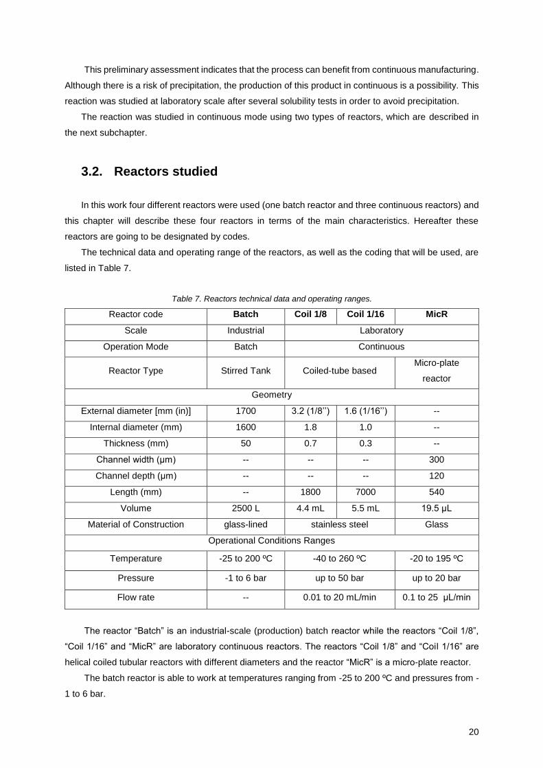
3.2. Reactors studied
In this work four different reactors were used (one batch reactor and three continuous reactors) and
this chapter will describe these four reactors in terms of the main characteristics. Hereafter these
reactors are going to be designated by codes.
The technical data and operating range of the reactors, as well as the coding that will be used, are
listed in Table 7.
Table 7. Reactors technical data and operating ranges.
Reactor code Batch Coil 1/8 Coil 1/16 MicR
Scale Industrial Laboratory
Operation Mode Batch Continuous
Reactor Type Stirred Tank Coiled-tube based Micro-plate
reactor
Geometry
External diameter [mm (in)] 1700 3.2 (1/8’’) 1.6 (1/16’’) --
Internal diameter (mm) 1600 1.8 1.0 --
Thickness (mm) 50 0.7 0.3 --
Channel width (μm) -- -- -- 300
Channel depth (μm) -- -- -- 120
Length (mm) -- 1800 7000 540
Volume 2500 L 4.4 mL 5.5 mL 19.5 μL
Material of Construction glass-lined stainless steel Glass
Operational Conditions Ranges
Temperature -25 to 200 ºC -40 to 260 ºC -20 to 195 ºC
Pressure -1 to 6 bar up to 50 bar up to 20 bar
Flow rate -- 0.01 to 20 mL/min 0.1 to 25 μL/min
The reactor “Batch” is an industrial-scale (production) batch reactor while the reactors “Coil 1/8”,
“Coil 1/16” and “MicR” are laboratory continuous reactors. The reactors “Coil 1/8” and “Coil 1/16” are
helical coiled tubular reactors with different diameters and the reactor “MicR” is a micro-plate reactor.
The batch reactor is able to work at temperatures ranging from -25 to 200 ºC and pressures from -
1 to 6 bar.
21
The temperature, pressure and flow rate of the coil reactors can vary in the range from -40 to
260 ºC, and from atmospheric pressure up to 50 bar and with flows from 0.01 to 20 mL/min. Concerning
MicR, the temperature can vary from -20 to 195 ºC, the pressure up to 20 bar and the flow rate from 0.1
to 25 μL/min.
3.3. Work Methodology
This work can be divided into three parts:
The evaluation of the reaction kinetics based on data from a production batch in the
industrial reactor.
The study of continuous laboratory reactors:
o Study I: Characterization of the reactors
o Study II: Kinetic studies
o Study III: Performance evaluation of laboratory continuous reactor by modeling.
The definition of a methodology for scaling-up continuous processes based on the
developed work.
When dealing with different scales of reactors, in particular when the reactor configuration varies
significantly, one of the major issues is to scale-up/scale-down the process without affecting its
performance (eg. quality of the final product, yield, etc.). With the aim of defining a scale-up/scale-down
methodology, independent of the continuous reactor type, it is important to decouple the effects due to
the reaction kinetics from the behavior of the reactor itself, both in terms of hydrodynamic flow and heat
transfer. With this purpose, the reactors were characterized, in terms of flow and heat transfer and the
kinetic parameters of the reaction were determined. With this approach, it will be possible to simulate
operational conditions of a specific reaction in different reactors and, therefore, anticipate its
performance.
The use of a batch reactor to characterize the reactions is relatively straightforward and, in this case,
it was used actual production data from industrial batch reactors.
In order to characterize the continuous coil reactors, residence time distributions were used to
assess the flow characteristics. Heat transfer was also experimentally investigated for these reactors.
The availability of kinetic data, from which, eventually, a kinetic model can be developed, is the starting
point for scaling up from laboratory to pilot plant reactors.
Scheme 1 represents schematically the work methodology followed in this work.
22
Scheme 1. Thesis work methodology
3.4. Experimental Characterization of Continuous Reactors
Characterization of the laboratory reactors was done based on the results of experimental tests:
Residence Time Distribution (RTD)
Heat Transfer
Kinetic studies
Table 8 summarizes the tests carried out in each continuous reactor.
Table 8. Characterization tests performed in each continuous reactor.
3.4.1. Residence Time Distribution Tests
The residence time distribution of a reactor is one of the most informative characterizations of real
continuous reactors. From the RTD it is possible to know how long the various elements have been in
the reactor. Each fluid element has a time, or age associated with it, which is defined as the time elapsed
since it entered the reactor. In other words, it determines the distribution of time spent inside the system
[42], [43].
Reactors
Tests Coil 1/8 Coil 1/16 MicR
RTD
Heat transfer
Kinetic
Dynamics of the Reactor - Reactor Performance:
Residence Time Distributions
Heat Transfer
Dynamics of the Reaction:
Reaction Kinetics
Results and Models
Models capable of simulating the process
Scale-Up Methodology proposal
23
In order to predict the behavior of a reaction-system, first it must be determined how long different
fluid elements remain in the reactor. This determination can be done experimentally with tracers, which
should be nonreactive, be easily detectable, show similar properties to those of the reacting mixture, be
completely soluble in the mixture and do not adsorb on any of the reactor components, in particular the
wall of the reactor itself [44], [45], [46].
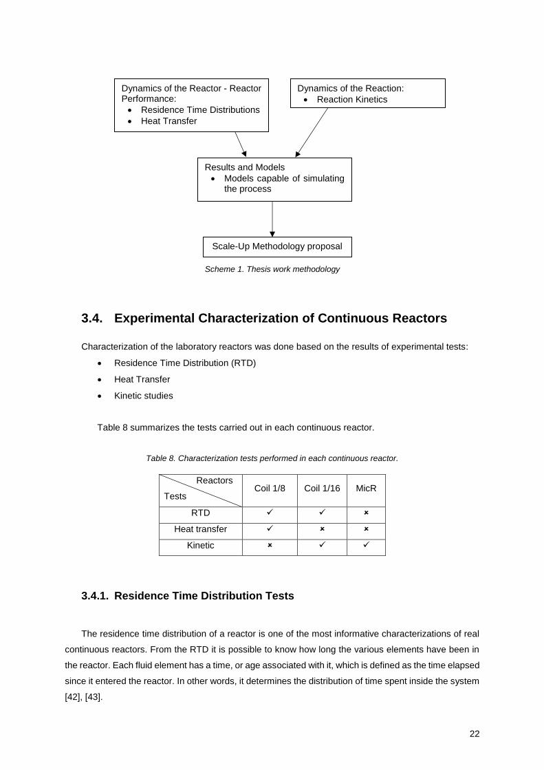
In this work, a colored tracer was injected as a pulse at the entrance of the tubular reactor and it
was detected at the exit using a diode-array spectrophotometer (UV-Vis spectrophotometer). The
concentration of the tracer was estimated from the absorbance at two wavelengths (295 and 520 nm),
according to the Lambert-Beer law.
As shown in Table 8, the RTD tests were only performed in the coil reactors. The procedure followed
was the same for the two reactors.
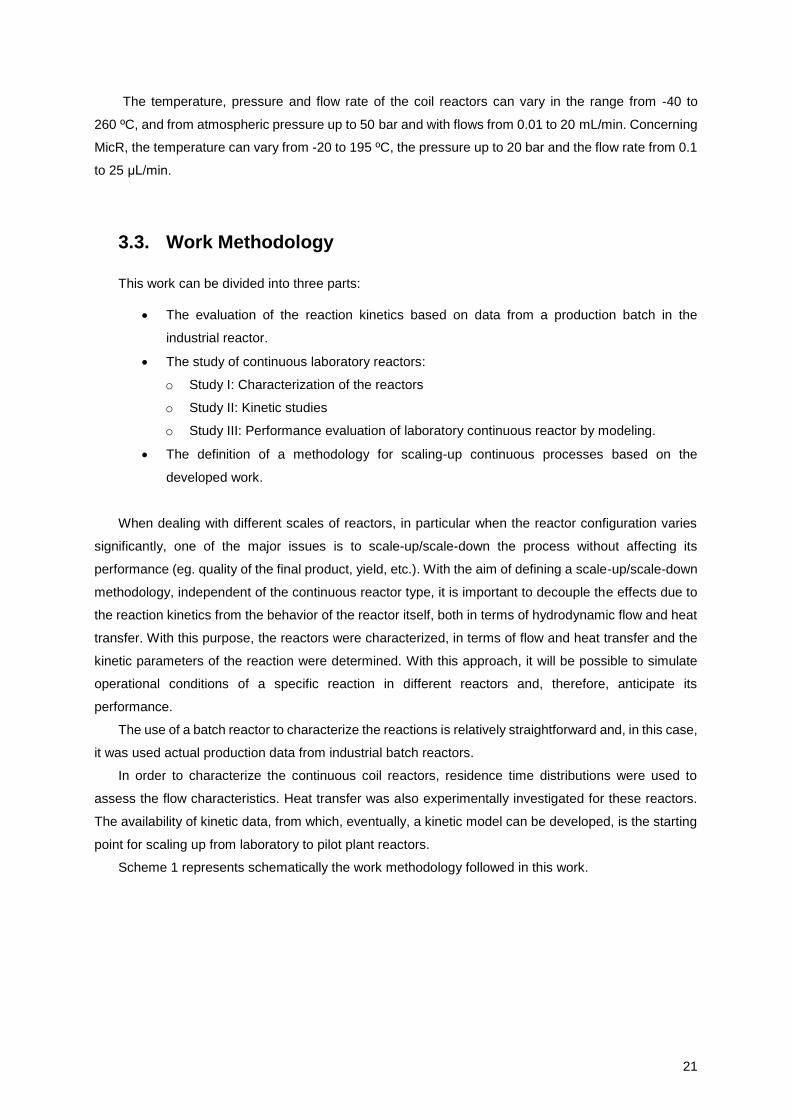
The RTD experiments were conducted using a coil reactor. A schematic diagram of the laboratory
setup is given in Figure 5.
UV-Vis
water
Tracer
Solution
Collector
HPLC
Pump
Coil Reactor
Figure 5. Schematic diagram of the setup for the residence time distribution tests.
The tests were performed with water. Ideally, the characterization tests should be performed using
the same solvent as the one used in the reaction, in this case, ethanol. Nevertheless, no significant
impact on results is expected as it can be considered that both solvents have similar properties.
The experiment was performed through the following procedure:
1. An HPLC pump was installed and a set of different flow rates were tested – 0.2, 1, 2, 4, 6 and
10 mL/min for coil 1/8 and 0.9, 1, 2, 4, 6 and 10 mL/min the coil 1/16;
2. A valve was changed from the water solution to the tracer solution and 1 mL of tracer was
injected into the feed stream in one shot (pulse input) by the HPLC pump. An aqueous solution
with dye was prepared to be used as a tracer;
3. The solution flowed into the coil reactor (coil 1/8 and coil 1/16);
4. The concentration of tracer was measured in the effluent stream over time. For that
measurement, an UV-Vis spectrometer was installed at the end of the set-up to measure the
absorbances of the tracer.
In order to select the best wavelength to collect the data, the UV-Vis spectrum of the tracer (Figure
6) was determined.
24
Figure 6. UV-Vis spectra of the tracer solution.
The two higher peaks seen in Figure 6 correspondent to a wavelength of 295 nm and 520 nm were
used to collected absorbances for the determination of tracer concentration.
3.4.2. Heat Transfer Tests
As summarized in Table 8, the heat transfer tests were only performed in the reactor coil 1/8. The
schematic diagram of the setup is shown in Figure 7.
water Collector
HPLC
Pump
Immersed Coil Reactor
TI
TITI
Figure 7. Schematic diagram of the setup for the heat transfer tests.
Water was selected as working fluid. Water at the ambient tempertaure flows through the tube and
hot water was in a stirred bath. The coil was submerged in the bath and temperatures at both inlet and
outlet of the coiled tube were measured as function of time by PT100 probes, represented in Figure 7
as TI (temperature indicator). These probes reading the reactor temperature were installed outside the
water bath.
Prior starting the experiments, a leakage test of the reactor was performed by filling it with water.
When the bath temperature became constant, the following procedure was carried out:
1. The HPLC pump started injecting water at the ambient temperature inside the coil;
2. The inlet and outlet temperatures were recorded every 30 seconds;
-0.002
0
0.002
0.004
0.006
0.008
0.01
0.012
0 200 400 600 800 1000
Abs
λ (nm)
295 nm 520 nm
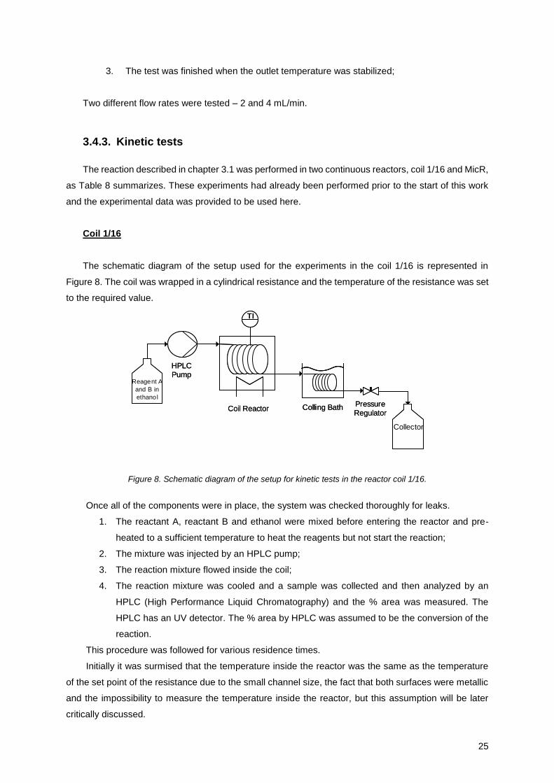
25
3. The test was finished when the outlet temperature was stabilized;
Two different flow rates were tested – 2 and 4 mL/min.
3.4.3. Kinetic tests
The reaction described in chapter 3.1 was performed in two continuous reactors, coil 1/16 and MicR,
as Table 8 summarizes. These experiments had already been performed prior to the start of this work
and the experimental data was provided to be used here.
Coil 1/16
The schematic diagram of the setup used for the experiments in the coil 1/16 is represented in
Figure 8. The coil was wrapped in a cylindrical resistance and the temperature of the resistance was set
to the required value.
Reagent A
and B in
ethanol
TI
Collector
Colling BathCoil Reactor
HPLC Pump
Pressure Regulator
Reagent A
and B in
ethanol
TI
Collector
Colling BathCoil Reactor
HPLC Pump
Pressure Regulator
Figure 8. Schematic diagram of the setup for kinetic tests in the reactor coil 1/16.
Once all of the components were in place, the system was checked thoroughly for leaks.
1. The reactant A, reactant B and ethanol were mixed before entering the reactor and pre-
heated to a sufficient temperature to heat the reagents but not start the reaction;
2. The mixture was injected by an HPLC pump;
3. The reaction mixture flowed inside the coil;
4. The reaction mixture was cooled and a sample was collected and then analyzed by an
HPLC (High Performance Liquid Chromatography) and the % area was measured. The
HPLC has an UV detector. The % area by HPLC was assumed to be the conversion of the
reaction.
This procedure was followed for various residence times.
Initially it was surmised that the temperature inside the reactor was the same as the temperature
of the set point of the resistance due to the small channel size, the fact that both surfaces were metallic
and the impossibility to measure the temperature inside the reactor, but this assumption will be later
critically discussed.
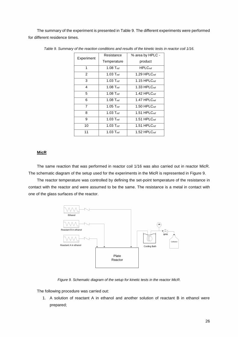
26
The summary of the experiment is presented in Table 9. The different experiments were performed
for different residence times.
Table 9. Summary of the reaction conditions and results of the kinetic tests in reactor coil 1/16.
Experiment Resistance
Temperature
% area by HPLC -
product
1 1.08 Tref HPLCref
2 1.03 Tref 1.29 HPLCref
3 1.03 Tref 1.15 HPLCref
4 1.08 Tref 1.33 HPLCref
5 1.08 Tref 1.42 HPLCref
6 1.08 Tref 1.47 HPLCref
7 1.05 Tref 1.50 HPLCref
8 1.03 Tref 1.51 HPLCref
9 1.03 Tref 1.51 HPLCref
10 1.03 Tref 1.51 HPLCref
11 1.03 Tref 1.52 HPLCref
MicR
The same reaction that was performed in reactor coil 1/16 was also carried out in reactor MicR.
The schematic diagram of the setup used for the experiments in the MicR is represented in Figure 9.
The reactor temperature was controlled by defining the set-point temperature of the resistance in
contact with the reactor and were assumed to be the same. The resistance is a metal in contact with
one of the glass surfaces of the reactor.
Ethanol
Reactant B in ethanol
Reactant A in ethanol
PI
BPR
Collector
Cooling Bath
Plate
Reactor
Figure 9. Schematic diagram of the setup for kinetic tests in the reactor MicR.
The following procedure was carried out:
1. A solution of reactant A in ethanol and another solution of reactant B in ethanol were
prepared;
27
2. The previous solutions were injected in the micro-reactor by syringe pumps;
3. The reaction mixture flowed inside the micro-reactor;
4. After the reaction ethanol was injected to dilute the mixture;
5. The reaction mixture was cooled in a cooling bath;
6. The reaction mixture was collected and a sample was then analyzed by an HPLC and the
% area was measured and assumed as the conversion of the reaction.
Table 10 summarizes the reaction conditions of the experiments carried out in reactor MicR.
Table 10. Summary of the reaction conditions and results of the kinetic tests in continuous MicR.
Experiment Resistance
Temperature % area by HPLC
1 0.82 Tref 0.05 HPLCref
2 Tref 0.18 HPLCref
3 0.82 Tref 0.16 HPLCref
4 Tref 0.45 HPLCref
5 0.82 Tref 0.34 HPLCref
6 Tref 1.06 HPLCref
7 Tref 1.43 HPLCref
3.5. Mathematical Tools
The relevant parameters in all the models applied in this work and which results discussion is
presented in next section, were estimated using the Solver tool of Excel. The parameters were optimized
in order to obtain a model as adjusted as possible to the experimental data. In order to do this, Solver
minimized the square of the difference between the values calculated by the model and the experimental
data, changing certain parameters. The objective function is expressed, in a generic way, in equation
(11).
Each model, and the parameters determined, are explained in detail in the next chapters.
𝑂𝑏𝑗𝑒𝑐𝑡𝑖𝑣𝑒 𝑓𝑢𝑛𝑐𝑡𝑖𝑜𝑛 = min {∑(𝑋𝑖𝑒𝑥𝑝
− 𝑋𝑖𝑚𝑜𝑑)2
𝑛
𝑖=0
} (11)
28
4. Experimental Results and Discussion
In this chapter it will be presented and discussed the results of the experiments performed in each
reactor divided per characterization tests.
4.1. Residence Time Distributions
Modeling of the reaction kinetics and a more detailed comparison between reactors with different
configurations can be studied by using RTD [3], [4], [43].
The distribution of residence times is represented by an exit age distribution function, E(t) dt, which
is defined as the fraction of material in the outlet stream that has been in the reactor for the period
between t and t+dt. All the fluid elements have some residence time, therefore, over a sufficiently long
period, all tracer will eventually come out. This is represented by equation (12) [44].
∫ 𝐸(𝑡)𝑑𝑡∞
0
= 1 (12)
The absorbance curve as a function of time was normalized by using the Simpson’s rule to compute
the overall integral and to obtain the residence time distribution according to equation (13).
𝐸(𝑡) = 𝐶(𝑡)
∫ 𝐶(𝑡)𝑑𝑡∞
0
(13)
The average time is given by the first moment of the age distribution as follows:
𝑡𝑚 = ∫ 𝑡 𝐸(𝑡)𝑑𝑡
∞
0
∫ 𝐸(𝑡)𝑑𝑡∞
0
= ∫ 𝑡 𝐸(𝑡)𝑑𝑡∞
0
(14)
If there are no stagnant volumes within the reactor then tm will be equal to θ, which is the quotient
between the reactor volume and the volumetric flow rate of the fluid, as shown in equation (15).
𝜃 =𝑉
𝑄𝑣 (15)
This equation also assumes that no significant by-pass flows are present as these are often hard
to detect using a pulse tracer injection.
To simplify, the residence time distributions are only going to be represented in this document for
the wavelength of 520 nm since it is the most intense absorbance peak (see Figure 6). The RTD for the
wavelength of 295 nm are in the Appendixes.
Applying the procedure described in subchapter 3.4.1, the residence time distribution functions
were obtained for the tubular reactors (coil 1/8 and coil 1/16) at several flow rates. The results obtained
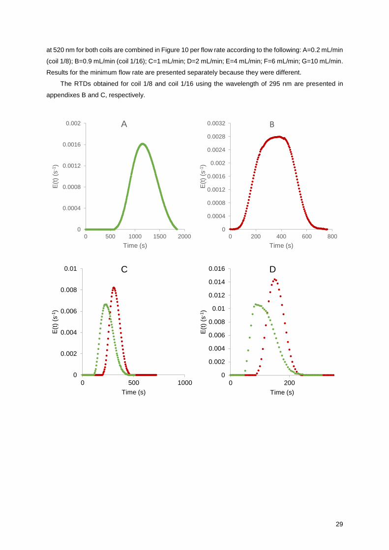
29
at 520 nm for both coils are combined in Figure 10 per flow rate according to the following: A=0.2 mL/min
(coil 1/8); B=0.9 mL/min (coil 1/16); C=1 mL/min; D=2 mL/min; E=4 mL/min; F=6 mL/min; G=10 mL/min.
Results for the minimum flow rate are presented separately because they were different.
The RTDs obtained for coil 1/8 and coil 1/16 using the wavelength of 295 nm are presented in
appendixes B and C, respectively.
0
0.0004
0.0008
0.0012
0.0016
0.002
0 500 1000 1500 2000
E(t
) (s
-1)
Time (s)
A
0
0.0004
0.0008
0.0012
0.0016
0.002
0.0024
0.0028
0.0032
0 200 400 600 800
E(t
) (s
-1)
Time (s)
B
0
0.002
0.004
0.006
0.008
0.01
0 500 1000
E(t
)(s
-1)
Time (s)
C
0
0.002
0.004
0.006
0.008
0.01
0.012
0.014
0.016
0 200
E(t
) (s
-1)
Time (s)
D
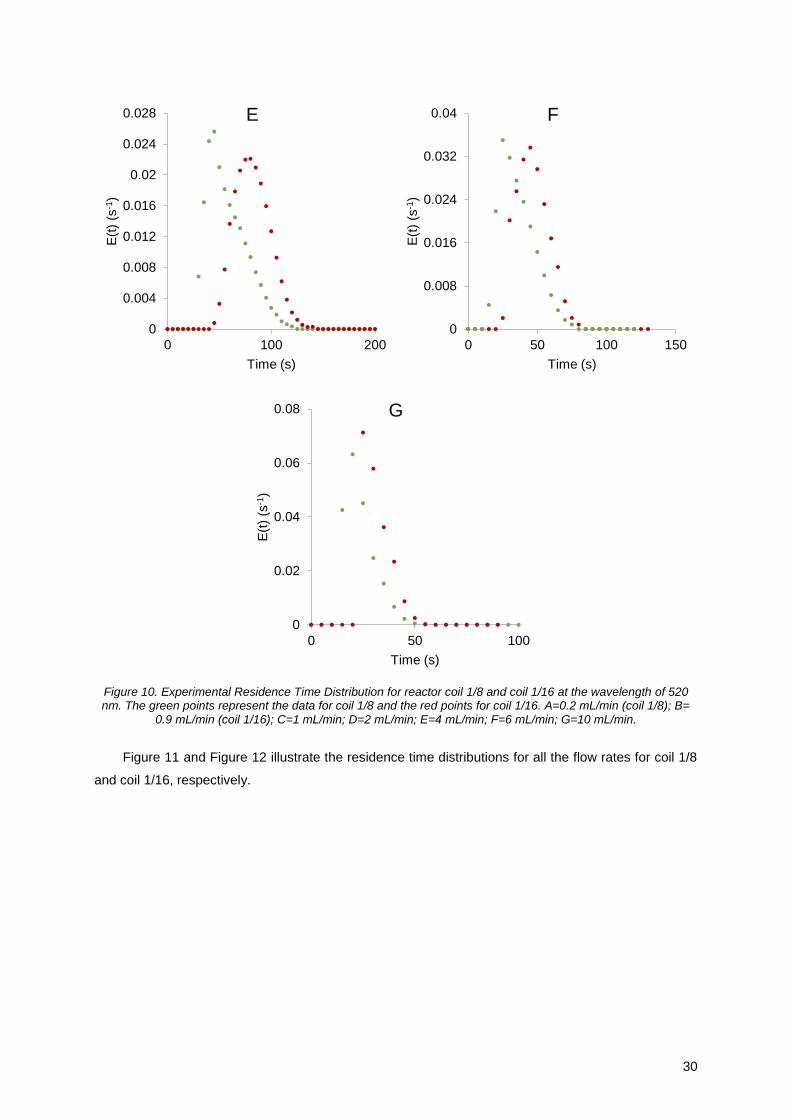
30
Figure 10. Experimental Residence Time Distribution for reactor coil 1/8 and coil 1/16 at the wavelength of 520 nm. The green points represent the data for coil 1/8 and the red points for coil 1/16. A=0.2 mL/min (coil 1/8); B=
0.9 mL/min (coil 1/16); C=1 mL/min; D=2 mL/min; E=4 mL/min; F=6 mL/min; G=10 mL/min.
Figure 11 and Figure 12 illustrate the residence time distributions for all the flow rates for coil 1/8
and coil 1/16, respectively.
0
0.004
0.008
0.012
0.016
0.02
0.024
0.028
0 100 200
E(t
)(s
-1)
Time (s)
E
0
0.008
0.016
0.024
0.032
0.04
0 50 100 150
E(t
)(s
-1)
Time (s)
F
0
0.02
0.04
0.06
0.08
0 50 100
E(t
)(s
-1)
Time (s)
G
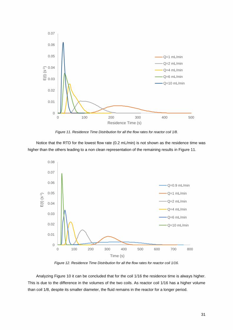
31
Figure 11. Residence Time Distribution for all the flow rates for reactor coil 1/8.
Notice that the RTD for the lowest flow rate (0.2 mL/min) is not shown as the residence time was
higher than the others leading to a non clean representation of the remaining results in Figure 11.
Figure 12. Residence Time Distribution for all the flow rates for reactor coil 1/16.
Analyzing Figure 10 it can be concluded that for the coil 1/16 the residence time is always higher.
This is due to the difference in the volumes of the two coils. As reactor coil 1/16 has a higher volume
than coil 1/8, despite its smaller diameter, the fluid remains in the reactor for a longer period.
0
0.01
0.02
0.03
0.04
0.05
0.06
0.07
0 100 200 300 400 500
E(t
) (s
-1)
Residence Time (s)
Q=1 mL/min
Q=2 mL/min
Q=4 mL/min
Q=6 mL/min
Q=10 mL/min
0
0.01
0.02
0.03
0.04
0.05
0.06
0.07
0.08
0 100 200 300 400 500 600 700 800
E(t
) (s
-1)
Time (s)
Q=0.9 mL/min
Q=1 mL/min
Q=2 mL/min
Q=4 mL/min
Q=6 mL/min
Q=10 mL/min
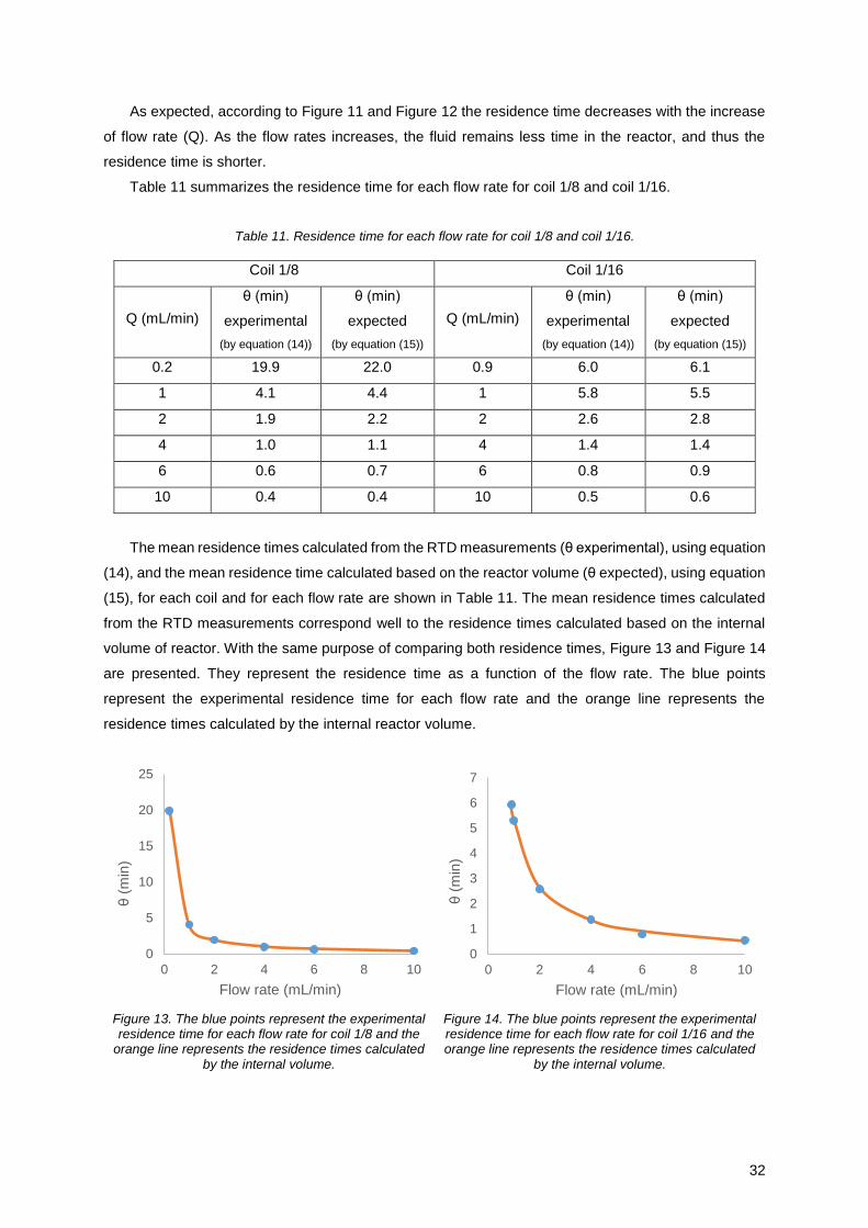
32
As expected, according to Figure 11 and Figure 12 the residence time decreases with the increase
of flow rate (Q). As the flow rates increases, the fluid remains less time in the reactor, and thus the
residence time is shorter.
Table 11 summarizes the residence time for each flow rate for coil 1/8 and coil 1/16.
Table 11. Residence time for each flow rate for coil 1/8 and coil 1/16.
Coil 1/8 Coil 1/16
Q (mL/min)
θ (min)
experimental
(by equation (14))
θ (min)
expected
(by equation (15))
Q (mL/min)
θ (min)
experimental
(by equation (14))
θ (min)
expected
(by equation (15))
0.2 19.9 22.0 0.9 6.0 6.1
1 4.1 4.4 1 5.8 5.5
2 1.9 2.2 2 2.6 2.8
4 1.0 1.1 4 1.4 1.4
6 0.6 0.7 6 0.8 0.9
10 0.4 0.4 10 0.5 0.6
The mean residence times calculated from the RTD measurements (θ experimental), using equation
(14), and the mean residence time calculated based on the reactor volume (θ expected), using equation
(15), for each coil and for each flow rate are shown in Table 11. The mean residence times calculated
from the RTD measurements correspond well to the residence times calculated based on the internal
volume of reactor. With the same purpose of comparing both residence times, Figure 13 and Figure 14
are presented. They represent the residence time as a function of the flow rate. The blue points
represent the experimental residence time for each flow rate and the orange line represents the
residence times calculated by the internal reactor volume.
Figure 13. The blue points represent the experimental residence time for each flow rate for coil 1/8 and the
orange line represents the residence times calculated by the internal volume.
Figure 14. The blue points represent the experimental residence time for each flow rate for coil 1/16 and the orange line represents the residence times calculated
by the internal volume.
0
5
10
15
20
25
0 2 4 6 8 10
θ(m
in)
Flow rate (mL/min)
0
1
2
3
4
5
6
7
0 2 4 6 8 10
θ(m
in)
Flow rate (mL/min)
33
As can be seen from the line in Figures 10 and 11 the data shows a high consistency, which
indicates that there are no significant changes in possible dead-volumes with the changes in flow-rate.
From the data presented, assuming that the measured flow-rates are accurate, the effective volume of
these two reactors are 4.0 mL and 5.3 mL, respectively for coil 1/8 and coil 1/16, which compare well
with the expected values of 4.4 mL and 5.5 mL indicated in Table 7.
However, the residence time distributions present some deviations from plug flow since they have
some width, showing a deviation from the ideality.
4.2. Heat Transfer
In this study, heat transfer rates were investigated at the moment when the outlet temperature
became momentarily stable. The temperature difference, ΔT, between inlet and outlet temperatures at
this moment was taken to calculate the total heat transfer rate Q as follows:
𝑄 = 𝑚 𝐶𝑝 𝛥𝑇 (16)
where m is the mass flow rate of water through the reactor and Cp is the specific heat capacity.
On the other hand, the log mean temperature difference ΔTln is calculated assuming no
temperature change in bath (hot water). Thus the overall heat transfer coefficient, U, is obtained as
follows:
𝑈 =𝑄
𝐴 𝛥𝑇𝑙𝑛 (17)
The log mean temperature difference, ΔTln, is calculated by equation (18).
𝛥𝑇𝑙𝑛 =
𝑇𝑐𝑜𝑖𝑙 𝑜𝑢𝑡 − 𝑇𝑐𝑜𝑖𝑙 𝑖𝑛
𝑙𝑛 (𝑇𝑏𝑎𝑡ℎ − 𝑇𝑐𝑜𝑖𝑙 𝑖𝑛
𝑇𝑏𝑎𝑡ℎ − 𝑇𝑐𝑜𝑖𝑙 𝑜𝑢𝑡)
(18)
In order to calculate the heat transfer coefficient, equations (16) to (18) were used, as discussed
above.
The average temperature of the inlet and outlet was calculated from the moment when the outlet
temperature became constant. These values and the other parameters to calculate the heat transfer
coefficient and the heat transfer itself are listed in Table 12.
Table 12. Parameters for the calculation of UA.
Flow rate= 2 mL/min Flow rate= 4 mL/min
T in (ºC) 26.8 26.0
T out (ºC) 56.7 59.9
T bath (ºC) 92.9 93.5
ΔTln (ºC) 49.7 48.6
Mass (kg/s) 3.33x10⁻⁵ 6.67x10⁻⁵
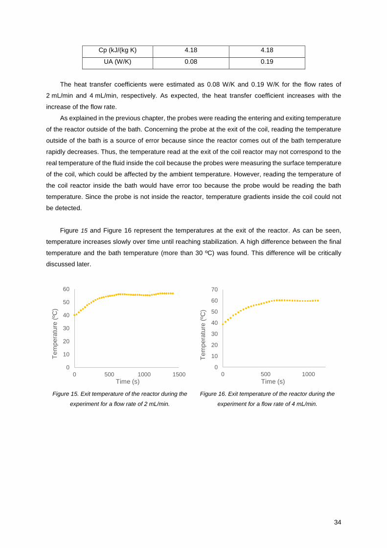
34
Cp (kJ/(kg K) 4.18 4.18
UA (W/K) 0.08 0.19
The heat transfer coefficients were estimated as 0.08 W/K and 0.19 W/K for the flow rates of
2 mL/min and 4 mL/min, respectively. As expected, the heat transfer coefficient increases with the
increase of the flow rate.
As explained in the previous chapter, the probes were reading the entering and exiting temperature
of the reactor outside of the bath. Concerning the probe at the exit of the coil, reading the temperature
outside of the bath is a source of error because since the reactor comes out of the bath temperature
rapidly decreases. Thus, the temperature read at the exit of the coil reactor may not correspond to the
real temperature of the fluid inside the coil because the probes were measuring the surface temperature
of the coil, which could be affected by the ambient temperature. However, reading the temperature of
the coil reactor inside the bath would have error too because the probe would be reading the bath
temperature. Since the probe is not inside the reactor, temperature gradients inside the coil could not
be detected.
Figure 15 and Figure 16 represent the temperatures at the exit of the reactor. As can be seen,
temperature increases slowly over time until reaching stabilization. A high difference between the final
temperature and the bath temperature (more than 30 ºC) was found. This difference will be critically
discussed later.
Figure 15. Exit temperature of the reactor during the
experiment for a flow rate of 2 mL/min.
Figure 16. Exit temperature of the reactor during the
experiment for a flow rate of 4 mL/min.
0
10
20
30
40
50
60
0 500 1000 1500
Tem
pera
ture
(ºC
)
Time (s)
0
10
20
30
40
50
60
70
0 500 1000
Tem
pera
ture
(ºC
)
Time (s)
35
5. Models Results and Discussion
This chapter describes in detail the development of the models applied to the characterization of the
reactors and for the determination of the kinetic data of the reaction under study and the hypothesis that
were used. Firstly it will be explained the model applied to the batch production data and then the models
for the continuous reactors.
5.1. Batch Reactor
In order to study the reaction carried out in a batch reactor and determine the kinetic parameters,
models based on mass and energy balances were fitted to the batch production data.
Briefly, the process consists in the following steps:
i. Reactant A, reactant B and solvent are charged into the reactor, in this order;
ii. The reaction mixture is heated to the required temperature;
iii. The reaction mixture is stirred for a long time;
iv. The reaction mixture is cooled and a sample is collected for an HPLC analysis and if
the content of the reactant A is within the in-process control limit (IPC), the process
proceeds to the next steps, otherwise, the reaction mixture has to be re-heated and
stirred for additional time until reaching the IPC limit.
Note that during the whole procedure the temperature of the reaction mixture is continuously
monitored and this is the data that is available for the development of the model.
The description of the evolution of the temperature profile within the reactor requires the model to
account both for the heat exchange with the surroundings (which provide heating and cooling) and the
heat involved in the reaction itself.
In order to get the model to adjust to the temperature profile of the reaction mixture and determine
the kinetic parameters, mass and energy balances had to be defined.
To remind, the reaction in study is of the type 𝐴 + 𝐵 → 𝐶 (𝑝𝑟𝑜𝑑𝑢𝑐𝑡) + 𝑠𝑢𝑏𝑝𝑟𝑜𝑑𝑢𝑐𝑡.
Mole Balance:
𝑑𝑛𝐴
𝑑𝑡= −𝑘𝐶𝐴𝐶𝐵𝑉
(19)
𝑑𝑛𝐵
𝑑𝑡= −𝑘𝐶𝐴𝐶𝐵𝑉
(20)
𝑑𝑛𝐶
𝑑𝑡= 𝑘𝐶𝐴𝐶𝐵𝑉
(21)
Energy Balance:
First, the general energy balance is presented in equation (22).
∑ 𝑛𝑖𝐶𝑝𝑖
𝑑𝑇
𝑑𝑡+ ∑
𝑑𝑛𝑖
𝑑𝑡𝐶𝑝𝑖(𝑇 − 𝑇𝑟𝑒𝑓) + ∑
𝑑𝑛𝑖
𝑑𝑡 𝛥𝐻𝑓𝑖
= 𝑈𝐴 (𝑇 − 𝑇𝑐𝑎𝑚𝑖𝑠𝑎) + ∑ 𝑄𝑖 𝐶𝑝𝑖 (𝑇𝑒 − 𝑇𝑟𝑒𝑓) + ∑ 𝐹𝑖∆𝐻𝑓𝑖
(22)
36
Since nothing is being added to the reactor, equation (22) can be re-written as:
∑ 𝑛𝑖𝐶𝑝𝑖
𝑑𝑇
𝑑𝑡+ ∑
𝑑𝑛𝑖
𝑑𝑡 𝛥𝐻𝑓𝑖 = 𝑈𝐴 (𝑇 − 𝑇𝑐𝑎𝑚𝑖𝑠𝑎)
(23)
which applied to the case study leads to:
∑ 𝑛𝑠𝑜𝑙𝑣𝑒𝑛𝑡 𝐶𝑝𝑠𝑜𝑙𝑣𝑒𝑛𝑡
𝑑𝑇
𝑑𝑡+ (−𝑘𝐶𝐴𝐶𝐵𝑉) 𝛥𝐻𝑓𝐴 + (−𝑘𝐶𝐴𝐶𝐵𝑉)𝛥𝐻𝑓𝐵
+ (𝑘𝐶𝐴𝐶𝐵𝑉𝛥𝐻𝑓𝐶 ) = 𝑈𝐴 (𝑇 − 𝑇𝑐𝑎𝑚𝑖𝑠𝑎)
(24)
Assuming that the variation in the sensible heat is predominantly due to the solvent and using an
average heat capacity of the reaction mixture, the final balance is given by equation (25).
𝑛𝑟𝑒𝑎𝑐𝑡𝑖𝑜𝑛 𝑚𝑖𝑥𝑡𝑢𝑟𝑒 𝐶𝑝𝑟𝑒𝑎𝑐𝑡𝑖𝑜𝑛 𝑚𝑖𝑥𝑡𝑢𝑟𝑒
𝑑𝑇
𝑑𝑡+ (−𝑟𝐴) 𝑉 𝛥𝐻𝑟 = 𝑈𝐴 (𝑇 − 𝑇𝑐𝑎𝑚𝑖𝑠𝑎) (25)
The set of differential equations was integrated using the Euler method with the following
rearrangements:
𝑑𝑇
𝑑𝑡=
𝑈𝐴 (𝑇 − 𝑇𝑐𝑎𝑚𝑖𝑠𝑎) − (−𝑟𝐴) 𝑉 𝛥𝐻𝑟
𝑛𝑟𝑒𝑎𝑐𝑡𝑖𝑜𝑛 𝑚𝑖𝑥𝑡𝑢𝑟𝑒 𝐶𝑝𝑟𝑒𝑎𝑐𝑡𝑖𝑜𝑛 𝑚𝑖𝑥𝑡𝑢𝑟𝑒
(26)
(−𝑟𝐴) = 𝑘0𝑒−𝐸𝑎/(𝑅𝑇)𝐶𝐴𝐶𝐵 (27)
The concentrations of A and B throughout the reaction, necessary for the reaction velocity, are also
given by the Euler method using the mass balance (Equations (28) and (29)).
𝑑𝐶𝐴
𝑑𝑡= −𝑘𝐶𝐴𝐶𝐵
(28)
𝑑𝐶𝐵
𝑑𝑡= −𝑘𝐶𝐴𝐶𝐵
(29)
The temperature that was calculated by the simultaneous integration of the four differential
equations, corresponding to the mass and energy balances, was fitted to the real temperature profile
during the reaction. This temperature profile is given by the temperature inside the reactor over the
whole period of reaction, i.e. heating, reaction time (isothermic conditions) and cooling. On the fitting
parameters that we wanted to obtain are: the pre-exponential factor (k0), the activation energy (Ea) and
the heat transfer coefficient (UA). Solver optimized these three parameters based on an objective
function based on the reactor temperature.
For confidentiality reasons, the temperature profile of the reaction cannot be presented, but Figure
17 shows the percentage error between the real reaction temperature and the temperature obtained
from the model. It can be concluded that the % error between the real reaction temperature and reaction
temperature obtained from the model is at maximum 15% and that model is not tendentious, describing
rather well the whole profile.
Table 13 summarizes the parameters determined from this model (k, Ea and UA).
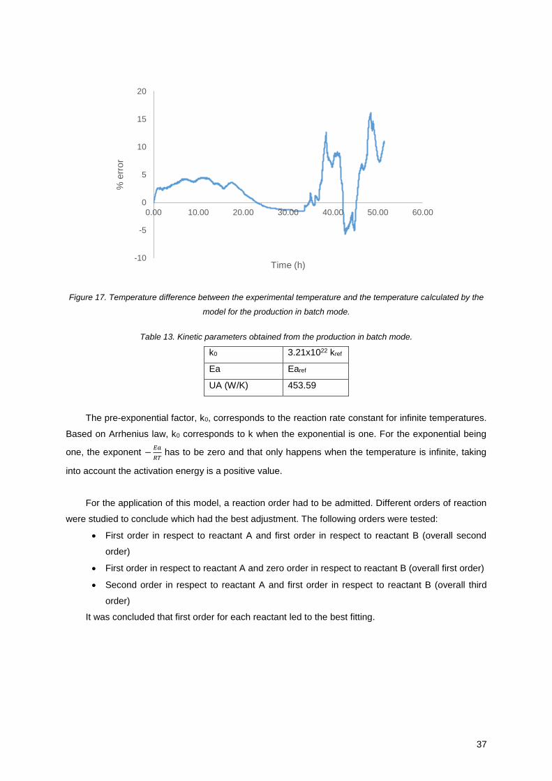
37
Figure 17. Temperature difference between the experimental temperature and the temperature calculated by the
model for the production in batch mode.
Table 13. Kinetic parameters obtained from the production in batch mode.
k0 3.21x10²² kref
Ea Earef
UA (W/K) 453.59
The pre-exponential factor, k0, corresponds to the reaction rate constant for infinite temperatures.
Based on Arrhenius law, k0 corresponds to k when the exponential is one. For the exponential being
one, the exponent −𝐸𝑎
𝑅𝑇 has to be zero and that only happens when the temperature is infinite, taking
into account the activation energy is a positive value.
For the application of this model, a reaction order had to be admitted. Different orders of reaction
were studied to conclude which had the best adjustment. The following orders were tested:
First order in respect to reactant A and first order in respect to reactant B (overall second
order)
First order in respect to reactant A and zero order in respect to reactant B (overall first order)
Second order in respect to reactant A and first order in respect to reactant B (overall third
order)
It was concluded that first order for each reactant led to the best fitting.
-10
-5
0
5
10
15
20
0.00 10.00 20.00 30.00 40.00 50.00 60.00
% e
rror
Time (h)
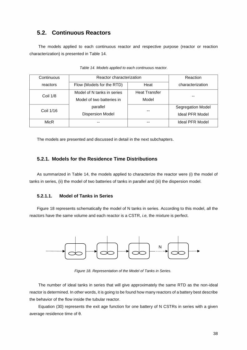
38
5.2. Continuous Reactors
The models applied to each continuous reactor and respective purpose (reactor or reaction
characterization) is presented in Table 14.
Table 14. Models applied to each continuous reactor.
Continuous
reactors
Reactor characterization Reaction
characterization Flow (Models for the RTD) Heat
Coil 1/8 Model of N tanks in series
Model of two batteries in
parallel
Dispersion Model
Heat Transfer
Model --
Coil 1/16 -- Segregation Model
Ideal PFR Model
MicR -- -- Ideal PFR Model
The models are presented and discussed in detail in the next subchapters.
5.2.1. Models for the Residence Time Distributions
As summarized in Table 14, the models applied to characterize the reactor were (i) the model of
tanks in series, (ii) the model of two batteries of tanks in parallel and (iii) the dispersion model.
5.2.1.1. Model of Tanks in Series
Figure 18 represents schematically the model of N tanks in series. According to this model, all the
reactors have the same volume and each reactor is a CSTR, i.e, the mixture is perfect.
The number of ideal tanks in series that will give approximately the same RTD as the non-ideal
reactor is determined. In other words, it is going to be found how many reactors of a battery best describe
the behavior of the flow inside the tubular reactor.
Equation (30) represents the exit age function for one battery of N CSTRs in series with a given
average residence time of θ.
N
Figure 18. Representation of the Model of Tanks in Series.
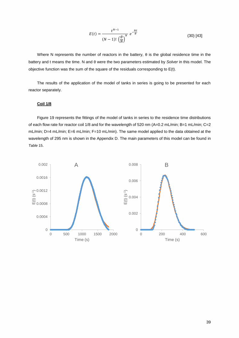
39
𝐸(𝑡) =𝑡𝑁−1
(𝑁 − 1)! (𝜃𝑁
)𝑁 𝑒
−𝑁𝑡𝜃
(30) [43]
Where N represents the number of reactors in the battery, θ is the global residence time in the
battery and t means the time. N and θ were the two parameters estimated by Solver in this model. The
objective function was the sum of the square of the residuals corresponding to E(t).
The results of the application of the model of tanks in series is going to be presented for each
reactor separately.
Coil 1/8
Figure 19 represents the fittings of the model of tanks in series to the residence time distributions
of each flow rate for reactor coil 1/8 and for the wavelength of 520 nm (A=0.2 mL/min; B=1 mL/min; C=2
mL/min; D=4 mL/min; E=6 mL/min; F=10 mL/min). The same model applied to the data obtained at the
wavelength of 295 nm is shown in the Appendix D. The main parameters of this model can be found in
Table 15.
0
0.0004
0.0008
0.0012
0.0016
0.002
0 500 1000 1500 2000
E(t
) (s
-1)
Time (s)
A
0
0.002
0.004
0.006
0.008
0 200 400 600
E(t
) (s
-1)
Time (s)
B
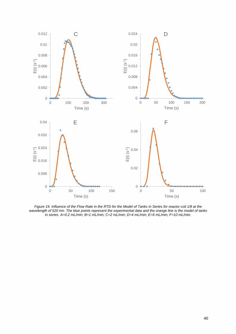
40
Figure 19. Influence of the Flow Rate in the RTD for the Model of Tanks in Series for reactor coil 1/8 at the wavelength of 520 nm. The blue points represent the experimental data and the orange line is the model of tanks
in series. A=0.2 mL/min; B=1 mL/min; C=2 mL/min; D=4 mL/min; E=6 mL/min; F=10 mL/min.
0
0.002
0.004
0.006
0.008
0.01
0.012
0 100 200 300
E(t
) (s
-1)
Time (s)
C
0
0.004
0.008
0.012
0.016
0.02
0.024
0 50 100 150 200
E(t
) (s
-1)
Time (s)
D
0
0.008
0.016
0.024
0.032
0.04
0 50 100 150
E(t
) (s
-1)
Time (s)
E
0
0.02
0.04
0.06
0 50 100
E(t
) (s
-1)
Time (s)
F
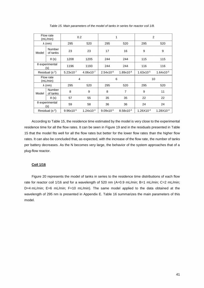
41
Table 15. Main parameters of the model of tanks in series for reactor coil 1/8.
According to Table 15, the residence time estimated by the model is very close to the experimental
residence time for all the flow rates. It can be seen in Figure 19 and in the residuals presented in Table
15 that the model fits well for all the flow rates but better for the lower flow rates than the higher flow
rates. It can also be concluded that, as expected, with the increase of the flow rate, the number of tanks
per battery decreases. As the N becomes very large, the behavior of the system approaches that of a
plug-flow reactor.
Coil 1/16
Figure 20 represents the model of tanks in series to the residence time distributions of each flow
rate for reactor coil 1/16 and for a wavelength of 520 nm (A=0.9 mL/min; B=1 mL/min; C=2 mL/min;
D=4 mL/min; E=6 mL/min; F=10 mL/min). The same model applied to the data obtained at the
wavelength of 295 nm is presented in Appendix E. Table 16 summarizes the main parameters of this
model.
Flow rate (mL/min)
0.2 1 2
λ (nm) 295 520 295 520 295 520
Model
Number of tanks
23 23 17 16 9 9
θ (s) 1208 1205 244 244 115 115
θ experimental
(s) 1196 1193 244 244 116 116
Residual (s-2) 5.23x10⁻⁷ 4.06x10⁻⁷ 2.54x10⁻⁶ 1.89x10⁻⁶ 1.63x10⁻⁵ 1.64x10⁻⁵
Flow rate (mL/min)
4 6 10
λ (nm) 295 520 295 520 295 520
Model
Number of tanks
8 9 8 7 9 11
θ (s) 57 55 35 35 22 22
θ experimental
(s) 59 58 36 36 24 24
Residual (s-2) 9.96x10⁻⁵ 1.24x10⁻⁴ 9.09x10⁻⁵ 8.58x10⁻⁵ 1.26X10⁻⁴ 1.28X10⁻⁴
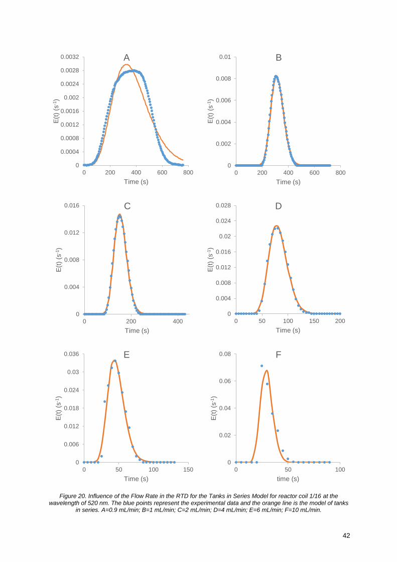
42
Figure 20. Influence of the Flow Rate in the RTD for the Tanks in Series Model for reactor coil 1/16 at the wavelength of 520 nm. The blue points represent the experimental data and the orange line is the model of tanks
in series. A=0.9 mL/min; B=1 mL/min; C=2 mL/min; D=4 mL/min; E=6 mL/min; F=10 mL/min.
0
0.0004
0.0008
0.0012
0.0016
0.002
0.0024
0.0028
0.0032
0 200 400 600 800
E(t
) (s
-1)
Time (s)
A
0
0.002
0.004
0.006
0.008
0.01
0 200 400 600 800
E(t
) (s
-1)
Time (s)
B
0
0.004
0.008
0.012
0.016
0 200 400
E(t
) (s
-1)
Time (s)
C
0
0.004
0.008
0.012
0.016
0.02
0.024
0.028
0 50 100 150 200
E(t
) (s
-1)
Time (s)
D
0
0.006
0.012
0.018
0.024
0.03
0.036
0 50 100 150
E(t
) (s
-1)
Time (s)
E
0
0.02
0.04
0.06
0.08
0 50 100
E(t
) (s
-1)
time (s)
F
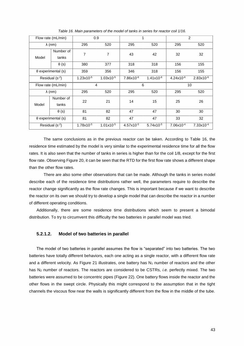
43
Table 16. Main parameters of the model of tanks in series for reactor coil 1/16.
The same conclusions as in the previous reactor can be taken. According to Table 16, the
residence time estimated by the model is very similar to the experimental residence time for all the flow
rates. It is also seen that the number of tanks in series is higher than for the coil 1/8, except for the first
flow rate. Observing Figure 20, it can be seen that the RTD for the first flow rate shows a different shape
than the other flow rates.
There are also some other observations that can be made. Although the tanks in series model
describe each of the residence time distributions rather well, the parameters require to describe the
reactor change significantly as the flow rate changes. This is important because if we want to describe
the reactor on its own we should try to develop a single model that can describe the reactor in a number
of different operating conditions.
Additionally, there are some residence time distributions which seem to present a bimodal
distribution. To try to circumvent this difficulty the two batteries in parallel model was tried.
5.2.1.2. Model of two batteries in parallel
The model of two batteries in parallel assumes the flow is “separated” into two batteries. The two
batteries have totally different behaviors, each one acting as a single reactor, with a different flow rate
and a different velocity. As Figure 21 illustrates, one battery has N1 number of reactors and the other
has N2 number of reactors. The reactors are considered to be CSTRs, i.e. perfectly mixed. The two
batteries were assumed to be concentric pipes (Figure 22). One battery flows inside the reactor and the
other flows in the swept circle. Physically this might correspond to the assumption that in the tight
channels the viscous flow near the walls is significantly different from the flow in the middle of the tube.
Flow rate (mL/min) 0.9 1 2
λ (nm) 295 520 295 520 295 520
Model
Number of
tanks 7 7 43 42 32 32
θ (s) 380 377 318 318 156 155
θ experimental (s) 359 356 346 318 156 155
Residual (s-2) 1.23x10⁻⁵ 1.03x10⁻⁵ 7.86x10⁻⁶ 1.41x10⁻⁶ 4.24x10⁻⁶ 2.83x10⁻⁶
Flow rate (mL/min) 4 6 10
λ (nm) 295 520 295 520 295 520
Model
Number of
tanks 22 21 14 15 25 26
θ (s) 81 82 47 47 30 30
θ experimental (s) 81 82 47 47 33 32
Residual (s-2) 1.78x10⁻⁵ 1.01x10⁻⁵ 4.57x10⁻⁵ 5.74x10⁻⁵ 7.06x10⁻⁴ 7.33x10⁻⁴
44
Figure 22. Illustration of the two concentric reactors (side and top view)
The expression of E(t) for two batteries in parallel is given by equation (31).
The parameters required to fit in this model were the number of tanks in each battery (N1 and N2),
the residence time in each battery (θ1 and θ2) and the ratio of flow rates flowing in each battery (Q1/Q
and Q2/Q, where Q= Q1+Q2). The objective function was the sum of the squares of the residuals of E(t).
Coil 1/8
Figure 23 represents the individual fittings of the model of two batteries in parallel to the RTD of each
flow rate for reactor coil 1/8 and for the wavelength of 520 nm (A=0.2 mL/min; B=1 mL/min; C=2 mL/min;
D=4 mL/min; E=6 mL/min; F=10 mL/min). The same model applied to the data obtained at the
wavelength of 295 nm is presented in Appendix F. Table 17 summarizes the main parameters of this
model.
𝐸(𝑡) =𝑡(𝑁1−1)
(𝑁1−1)! (𝜃1𝑁1
)𝑁1
𝑒−𝑁1𝑡
𝜃1 𝑄1
𝑄+
𝑡(𝑁2−1)
(𝑁2−1)! (𝜃2𝑁2
)𝑁2
𝑒−𝑁2𝑡
𝜃2 𝑄2
𝑄 (31) [43]
Q1
Q2
Q2
2
1
r
R
N1
N2
Figure 21. Representation of the Model of two batteries in parallel.
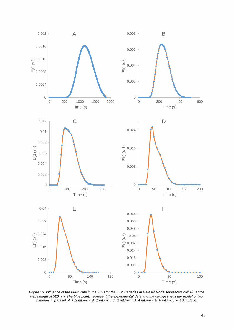
45
Figure 23. Influence of the Flow Rate in the RTD for the Two Batteries in Parallel Model for reactor coil 1/8 at the wavelength of 520 nm. The blue points represent the experimental data and the orange line is the model of two
batteries in parallel. A=0.2 mL/min; B=1 mL/min; C=2 mL/min; D=4 mL/min; E=6 mL/min; F=10 mL/min.
0
0.0004
0.0008
0.0012
0.0016
0.002
0 500 1000 1500 2000
E(t
)(s
-1)
Time (s)
A
0
0.002
0.004
0.006
0.008
0 200 400 600
E(t
)(s
-1)
Time (s)
B
0
0.002
0.004
0.006
0.008
0.01
0.012
0 100 200 300
E(t
)(s
-1)
Time (s)
C
0
0.008
0.016
0.024
0 50 100 150 200
E(t
) (s
-1)
Time (s)
D
0
0.008
0.016
0.024
0.032
0.04
0 50 100 150
E(t
)(s
-1)
Time (s)
E
0
0.008
0.016
0.024
0.032
0.04
0.048
0.056
0.064
0 50 100
E(t
)(s
-1)
Time (s)
F
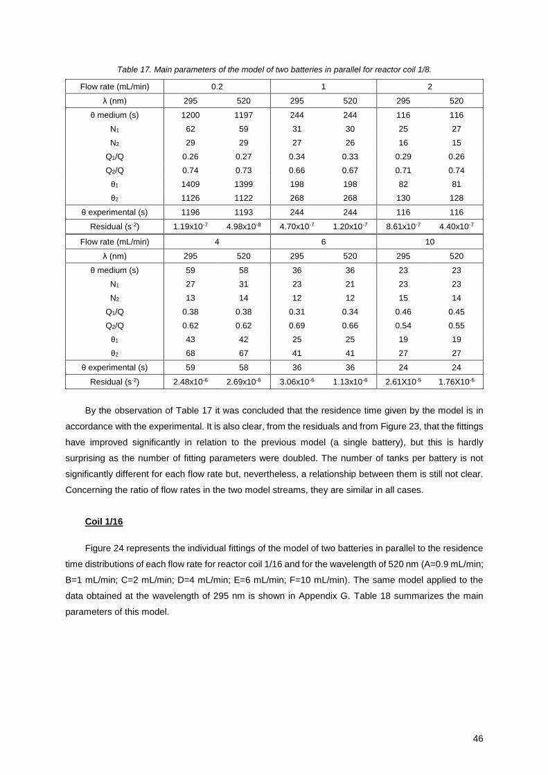
46
Table 17. Main parameters of the model of two batteries in parallel for reactor coil 1/8.
Flow rate (mL/min) 0.2 1 2
λ (nm) 295 520 295 520 295 520
θ medium (s) 1200 1197 244 244 116 116
N1 62 59 31 30 25 27
N2 29 29 27 26 16 15
Q1/Q 0.26 0.27 0.34 0.33 0.29 0.26
Q2/Q 0.74 0.73 0.66 0.67 0.71 0.74
θ1 1409 1399 198 198 82 81
θ2 1126 1122 268 268 130 128
θ experimental (s) 1196 1193 244 244 116 116
Residual (s-2) 1.19x10⁻⁷ 4.98x10⁻⁸ 4.70x10⁻⁷ 1.20x10⁻⁷ 8.61x10⁻⁷ 4.40x10⁻⁷
Flow rate (mL/min) 4 6 10
λ (nm) 295 520 295 520 295 520
θ medium (s) 59 58 36 36 23 23
N1 27 31 23 21 23 23
N2 13 14 12 12 15 14
Q1/Q 0.38 0.38 0.31 0.34 0.46 0.45
Q2/Q 0.62 0.62 0.69 0.66 0.54 0.55
θ1 43 42 25 25 19 19
θ2 68 67 41 41 27 27
θ experimental (s) 59 58 36 36 24 24
Residual (s-2) 2.48x10⁻⁶ 2.69x10⁻⁶ 3.06x10⁻⁶ 1.13x10⁻⁶ 2.61X10⁻⁵ 1.76X10⁻⁵
By the observation of Table 17 it was concluded that the residence time given by the model is in
accordance with the experimental. It is also clear, from the residuals and from Figure 23, that the fittings
have improved significantly in relation to the previous model (a single battery), but this is hardly
surprising as the number of fitting parameters were doubled. The number of tanks per battery is not
significantly different for each flow rate but, nevertheless, a relationship between them is still not clear.
Concerning the ratio of flow rates in the two model streams, they are similar in all cases.
Coil 1/16
Figure 24 represents the individual fittings of the model of two batteries in parallel to the residence
time distributions of each flow rate for reactor coil 1/16 and for the wavelength of 520 nm (A=0.9 mL/min;
B=1 mL/min; C=2 mL/min; D=4 mL/min; E=6 mL/min; F=10 mL/min). The same model applied to the
data obtained at the wavelength of 295 nm is shown in Appendix G. Table 18 summarizes the main
parameters of this model.
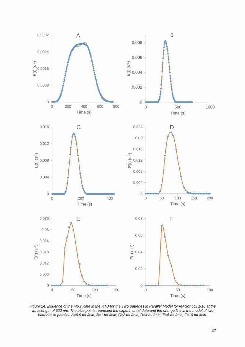
47
Figure 24. Influence of the Flow Rate in the RTD for the Two Batteries in Parallel Model for reactor coil 1/16 at the wavelength of 520 nm. The blue points represent the experimental data and the orange line is the model of two
batteries in parallel. A=0.9 mL/min; B=1 mL/min; C=2 mL/min; D=4 mL/min; E=6 mL/min; F=10 mL/min.
0
0.0008
0.0016
0.0024
0.0032
0 200 400 600 800
E(t
)(s
-1)
Time (s)
A
0
0.002
0.004
0.006
0.008
0 500 1000
E(t
)(s
-1)
Time (s)
B
0
0.004
0.008
0.012
0.016
0 200 400
E(t
)(s
-1)
Time (s)
C
0
0.004
0.008
0.012
0.016
0.02
0.024
0 50 100 150 200
E(t
)(s
-1)
Time (s)
D
0
0.006
0.012
0.018
0.024
0.03
0.036
0 50 100 150
E(t
)(s
-1)
Time (s)
E
0
0.02
0.04
0.06
0.08
0 50 100
E(t
)(s
-1)
Time (s)
F
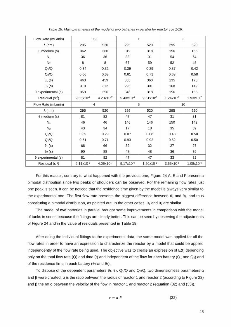
48
Table 18. Main parameters of the model of two batteries in parallel for reactor coil 1/16.
Flow Rate (mL/min) 0.9 1 2
λ (nm) 295 520 295 520 295 520
θ medium (s) 362 360 319 318 156 155
N1 36 36 88 91 54 64
N2 8 8 67 59 52 45
Q1/Q 0.34 0.32 0.39 0.29 0.37 0.42
Q2/Q 0.66 0.68 0.61 0.71 0.63 0.58
θ1 (s) 463 459 355 360 135 173
θ2 (s) 310 312 295 301 168 142
θ experimental (s) 359 356 346 318 156 155
Residual (s-2) 9.55x10⁻⁷ 4.23x10⁻⁷ 5.43x10⁻⁶ 9.61x10⁻⁸ 1.24x10⁻⁶ 1.93x10⁻⁷
Flow Rate (mL/min) 4 6 10
λ (nm) 295 520 295 520 295 520
θ medium (s) 81 82 47 47 31 31
N1 46 46 146 146 150 142
N2 43 34 17 18 35 39
Q1/Q 0.39 0.29 0.07 0.08 0.48 0.50
Q2/Q 0.61 0.71 0.93 0.92 0.52 0.50
θ1 (s) 68 66 32 32 27 27
θ2 (s) 90 88 48 48 36 35
θ experimental (s) 81 82 47 47 33 32
Residual (s-2) 2.11x10⁻⁶ 4.06x10⁻⁷ 9.17x10⁻⁶ 1.20x10⁻⁵ 3.55x10⁻⁶ 1.08x10⁻⁶
For this reactor, contrary to what happened with the previous one, Figure 24 A, E and F present a
bimodal distribution since two peaks or shoulders can be observed. For the remaining flow rates just
one peak is seen. It can be noticed that the residence time given by the model is always very similar to
the experimental one. The first flow rate presents the biggest difference between θ1 and θ2, and thus
constituting a bimodal distribution, as pointed out. In the other cases, θ1 and θ2 are similar.
The model of two batteries in parallel brought some improvements in comparison with the model
of tanks in series because the fittings are clearly better. This can be seen by observing the adjustments
of Figure 24 and in the value of residuals presented in Table 18.
After doing the individual fittings to the experimental data, the same model was applied for all the
flow rates in order to have an expression to characterize the reactor by a model that could be applied
independently of the flow rate being used. The objective was to create an expression of E(t) depending
only on the total flow rate (Q) and time (t) and independent of the flow for each battery (Q1 and Q2) and
of the residence time in each battery (θ1 and θ2).
To dispose of the dependent parameters θ1, θ2, Q1/Q and Q2/Q, two dimensionless parameters α
and β were created. α is the ratio between the radius of reactor 1 and reactor 2 (according to Figure 22)
and β the ratio between the velocity of the flow in reactor 1 and reactor 2 (equation (32) and (33)).
𝑟 = 𝛼 𝑅 (32)
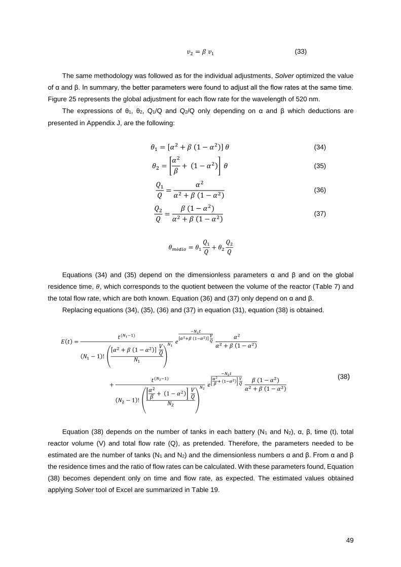
49
𝑣2 = 𝛽 𝑣1 (33)
The same methodology was followed as for the individual adjustments, Solver optimized the value
of α and β. In summary, the better parameters were found to adjust all the flow rates at the same time.
Figure 25 represents the global adjustment for each flow rate for the wavelength of 520 nm.
The expressions of θ1, θ2, Q1/Q and Q2/Q only depending on α and β which deductions are
presented in Appendix J, are the following:
𝜃1 = [𝛼2 + 𝛽 (1 − 𝛼2)] 𝜃 (34)
𝜃2 = [𝛼2
𝛽+ (1 − 𝛼2)] 𝜃 (35)
𝑄1
𝑄=
𝛼2
𝛼2 + 𝛽 (1 − 𝛼2) (36)
𝑄2
𝑄=
𝛽 (1 − 𝛼2)
𝛼2 + 𝛽 (1 − 𝛼2) (37)
𝜃𝑚é𝑑𝑖𝑜 = 𝜃1
𝑄1
𝑄+ 𝜃2
𝑄2
𝑄
Equations (34) and (35) depend on the dimensionless parameters α and β and on the global
residence time, 𝜃, which corresponds to the quotient between the volume of the reactor (Table 7) and
the total flow rate, which are both known. Equation (36) and (37) only depend on α and β.
Replacing equations (34), (35), (36) and (37) in equation (31), equation (38) is obtained.
𝐸(𝑡) =𝑡(𝑁1−1)
(𝑁1 − 1)! ([𝛼2 + 𝛽 (1 − 𝛼2)]
𝑉𝑄
𝑁1)
𝑁1 𝑒
−𝑁1𝑡
[𝛼2+𝛽 (1−𝛼2)] 𝑉𝑄
𝛼2
𝛼2 + 𝛽 (1 − 𝛼2)
+𝑡(𝑁2−1)
(𝑁2 − 1)! ([𝛼2
𝛽+ (1 − 𝛼2)]
𝑉𝑄
𝑁2)
𝑁2 𝑒
−𝑁2𝑡
[𝛼2
𝛽+ (1−𝛼2)]
𝑉𝑄
𝛽 (1 − 𝛼2)
𝛼2 + 𝛽 (1 − 𝛼2)
(38)
Equation (38) depends on the number of tanks in each battery (N1 and N2), α, β, time (t), total
reactor volume (V) and total flow rate (Q), as pretended. Therefore, the parameters needed to be
estimated are the number of tanks (N1 and N2) and the dimensionless numbers α and β. From α and β
the residence times and the ratio of flow rates can be calculated. With these parameters found, Equation
(38) becomes dependent only on time and flow rate, as expected. The estimated values obtained
applying Solver tool of Excel are summarized in Table 19.
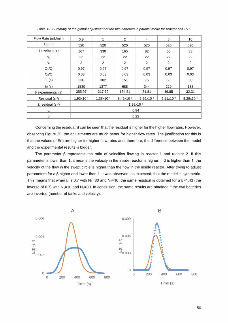
50
Table 19. Summary of the global adjustment of the two batteries in parallel mode for reactor coil 1/16.
Flow Rate (mL/min) 0.9 1 2 4 6 10
λ (nm) 520 520 520 520 520 520
θ medium (s) 367 330 165 82 55 33
N1 22 22 22 22 22 22
N2 2 2 2 2 2 2
Q1/Q 0.97 0.97 0.97 0.97 0.97 0.97
Q2/Q 0.03 0.03 0.03 0.03 0.03 0.03
θ1 (s) 336 302 151 76 50 30
θ2 (s) 1530 1377 688 344 229 138
θ experimental (s) 355.97 317.79 154.81 81.81 46.85 32.31
Residual (s-2) 1.93x10⁻⁴ 1.38x10⁻⁴ 8.49x10⁻⁵ 2.26x10⁻⁴ 5.11x10⁻⁴ 8.29x10⁻⁴
Σ residual (s-2) 1.98x10⁻³
α 0.94
β 0.22
Concerning the residual, it can be seen that the residual is higher for the higher flow rates. However,
observing Figure 25, the adjustments are much better for higher flow rates. The justification for this is
that the values of E(t) are higher for higher flow rates and, therefore, the difference between the model
and the experimental results is bigger.
The parameter β represents the ratio of velocities flowing in reactor 1 and reactor 2. If this
parameter is lower than 1, it means the velocity in the inside reactor is higher. If β is higher than 1, the
velocity of the flow in the swept circle is higher than the flow in the inside reactor. After trying to adjust
parameters for a β higher and lower than 1, it was observed, as expected, that the model is symmetric.
This means that when β is 0.7 with N1=30 and N2=10, the same residual is obtained for a β=1.43 (the
inverse of 0.7) with N1=10 and N2=30. In conclusion, the same results are obtained if the two batteries
are inverted (number of tanks and velocity).
0
0.002
0.004
0.006
0 200 400 600 800
E(t
)(s
-1)
Time (s)
A
0
0.003
0.006
0.009
0 200 400 600 800
E(t
)(s
-1)
Time (s)
B
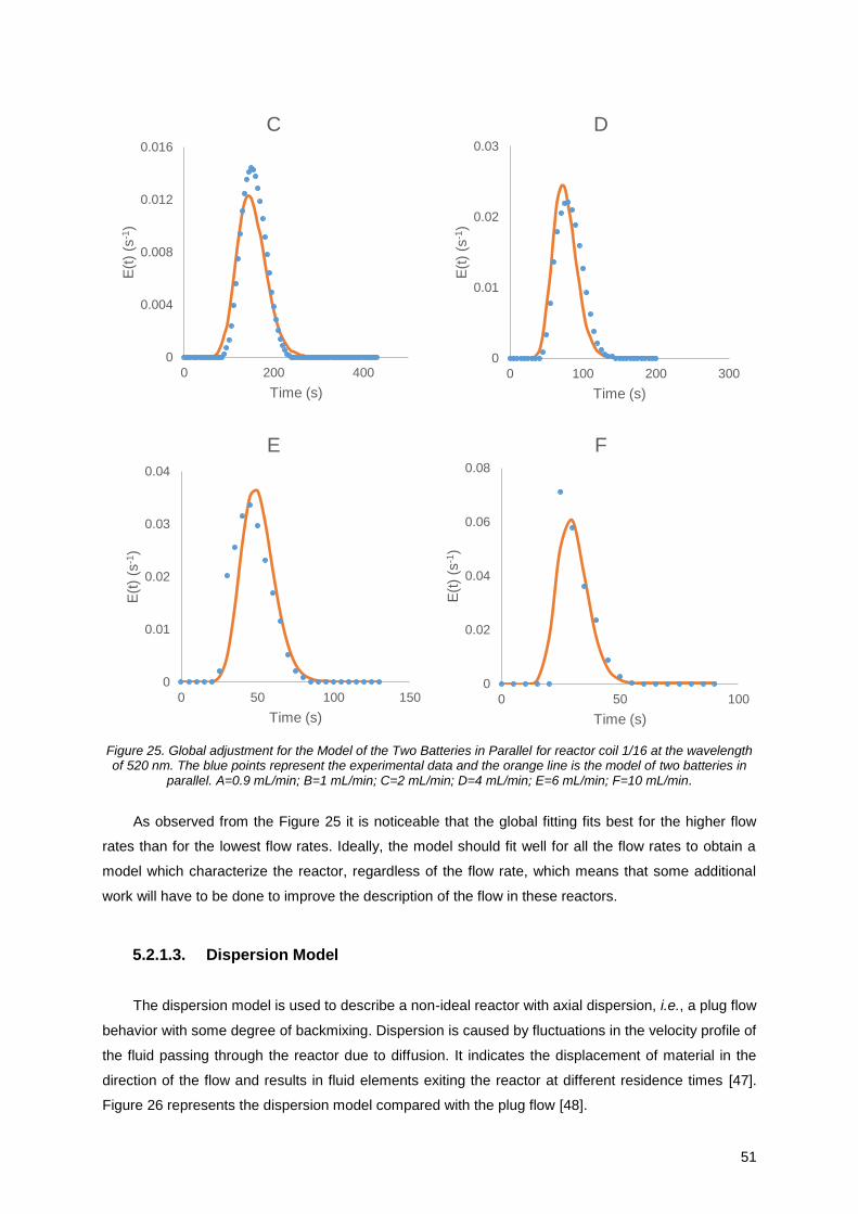
51
Figure 25. Global adjustment for the Model of the Two Batteries in Parallel for reactor coil 1/16 at the wavelength of 520 nm. The blue points represent the experimental data and the orange line is the model of two batteries in
parallel. A=0.9 mL/min; B=1 mL/min; C=2 mL/min; D=4 mL/min; E=6 mL/min; F=10 mL/min.
As observed from the Figure 25 it is noticeable that the global fitting fits best for the higher flow
rates than for the lowest flow rates. Ideally, the model should fit well for all the flow rates to obtain a
model which characterize the reactor, regardless of the flow rate, which means that some additional
work will have to be done to improve the description of the flow in these reactors.
5.2.1.3. Dispersion Model
The dispersion model is used to describe a non-ideal reactor with axial dispersion, i.e., a plug flow
behavior with some degree of backmixing. Dispersion is caused by fluctuations in the velocity profile of
the fluid passing through the reactor due to diffusion. It indicates the displacement of material in the
direction of the flow and results in fluid elements exiting the reactor at different residence times [47].
Figure 26 represents the dispersion model compared with the plug flow [48].
0
0.004
0.008
0.012
0.016
0 200 400
E(t
)(s
-1)
Time (s)
C
0
0.01
0.02
0.03
0 100 200 300
E(t
)(s
-1)
Time (s)
D
0
0.01
0.02
0.03
0.04
0 50 100 150
E(t
)(s
-1)
Time (s)
E
0
0.02
0.04
0.06
0.08
0 50 100
E(t
)(s
-1)
Time (s)
F
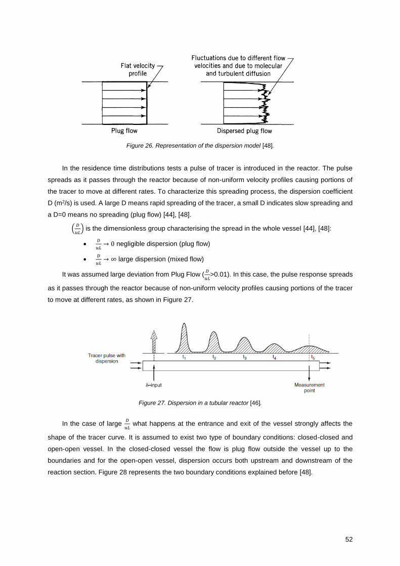
52
Figure 26. Representation of the dispersion model [48].
In the residence time distributions tests a pulse of tracer is introduced in the reactor. The pulse
spreads as it passes through the reactor because of non-uniform velocity profiles causing portions of
the tracer to move at different rates. To characterize this spreading process, the dispersion coefficient
D (m2/s) is used. A large D means rapid spreading of the tracer, a small D indicates slow spreading and
a D=0 means no spreading (plug flow) [44], [48].
(𝐷
𝑢𝐿) is the dimensionless group characterising the spread in the whole vessel [44], [48]:
𝐷
𝑢𝐿→ 0 negligible dispersion (plug flow)
𝐷
𝑢𝐿→ ∞ large dispersion (mixed flow)
It was assumed large deviation from Plug Flow (𝐷
𝑢𝐿>0.01). In this case, the pulse response spreads
as it passes through the reactor because of non-uniform velocity profiles causing portions of the tracer
to move at different rates, as shown in Figure 27.
Figure 27. Dispersion in a tubular reactor [46].
In the case of large 𝐷
𝑢𝐿 what happens at the entrance and exit of the vessel strongly affects the
shape of the tracer curve. It is assumed to exist two type of boundary conditions: closed-closed and
open-open vessel. In the closed-closed vessel the flow is plug flow outside the vessel up to the
boundaries and for the open-open vessel, dispersion occurs both upstream and downstream of the
reaction section. Figure 28 represents the two boundary conditions explained before [48].
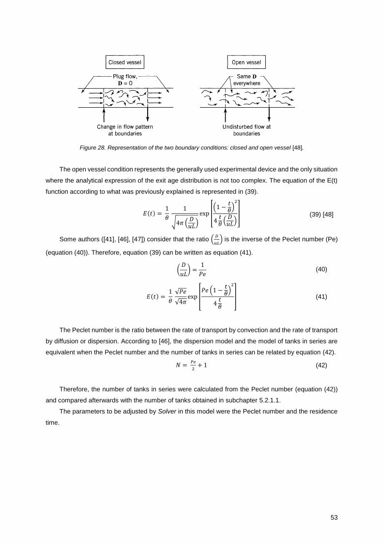
53
Figure 28. Representation of the two boundary conditions: closed and open vessel [48].
The open vessel condition represents the generally used experimental device and the only situation
where the analytical expression of the exit age distribution is not too complex. The equation of the E(t)
function according to what was previously explained is represented in (39).
𝐸(𝑡) = 1
𝜃
1
√4𝜋 (𝐷𝑢𝐿
)
exp [(1 −
𝑡𝜃
)2
4𝑡𝜃
(𝐷𝑢𝐿
)] (39) [48]
Some authors ([41], [46], [47]) consider that the ratio (𝐷
𝑢𝐿) is the inverse of the Peclet number (Pe)
(equation (40)). Therefore, equation (39) can be written as equation (41).
(𝐷
𝑢𝐿) =
1
𝑃𝑒 (40)
𝐸(𝑡) = 1
𝜃 √𝑃𝑒
√4𝜋exp [
𝑃𝑒 (1 −𝑡𝜃
)2
4𝑡𝜃
] (41)
The Peclet number is the ratio between the rate of transport by convection and the rate of transport
by diffusion or dispersion. According to [46], the dispersion model and the model of tanks in series are
equivalent when the Peclet number and the number of tanks in series can be related by equation (42).
𝑁 = 𝑃𝑒
2+ 1 (42)
Therefore, the number of tanks in series were calculated from the Peclet number (equation (42))
and compared afterwards with the number of tanks obtained in subchapter 5.2.1.1.
The parameters to be adjusted by Solver in this model were the Peclet number and the residence
time.
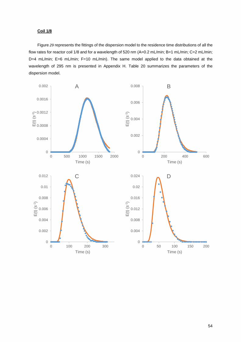
54
Coil 1/8
Figure 29 represents the fittings of the dispersion model to the residence time distributions of all the
flow rates for reactor coil 1/8 and for a wavelength of 520 nm (A=0.2 mL/min; B=1 mL/min; C=2 mL/min;
D=4 mL/min; E=6 mL/min; F=10 mL/min). The same model applied to the data obtained at the
wavelength of 295 nm is presented in Appendix H. Table 20 summarizes the parameters of the
dispersion model.
0
0.0004
0.0008
0.0012
0.0016
0.002
0 500 1000 1500 2000
E(t
)(s
-1)
Time (s)
A
0
0.002
0.004
0.006
0.008
0 200 400 600
E(t
)(s
-1)
Time (s)
B
0
0.002
0.004
0.006
0.008
0.01
0.012
0 100 200 300
E(t
)(s
-1)
Time (s)
C
0
0.004
0.008
0.012
0.016
0.02
0.024
0 50 100 150 200
E(t
)(s
-1)
Time (s)
D
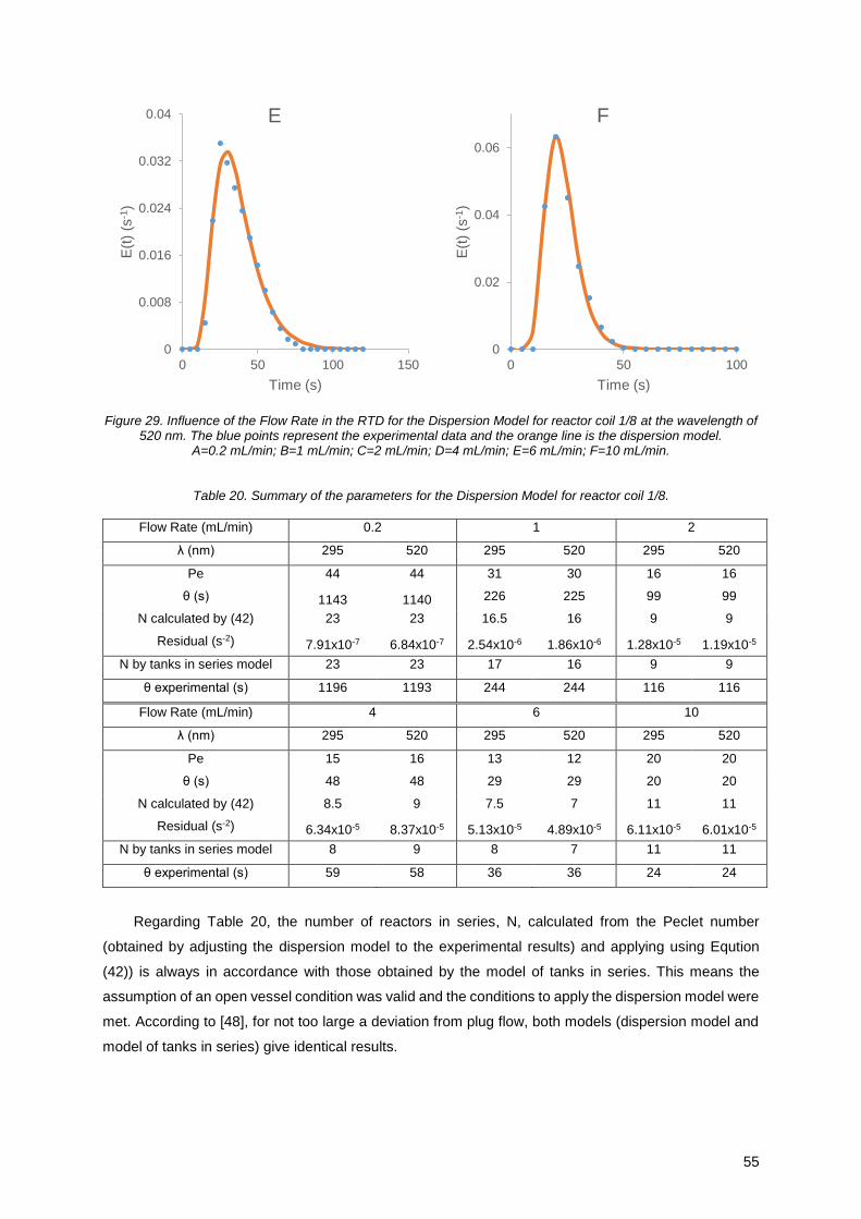
55
Figure 29. Influence of the Flow Rate in the RTD for the Dispersion Model for reactor coil 1/8 at the wavelength of 520 nm. The blue points represent the experimental data and the orange line is the dispersion model.
A=0.2 mL/min; B=1 mL/min; C=2 mL/min; D=4 mL/min; E=6 mL/min; F=10 mL/min.
Table 20. Summary of the parameters for the Dispersion Model for reactor coil 1/8.
Regarding Table 20, the number of reactors in series, N, calculated from the Peclet number
(obtained by adjusting the dispersion model to the experimental results) and applying using Eqution
(42)) is always in accordance with those obtained by the model of tanks in series. This means the
assumption of an open vessel condition was valid and the conditions to apply the dispersion model were
met. According to [48], for not too large a deviation from plug flow, both models (dispersion model and
model of tanks in series) give identical results.
Flow Rate (mL/min) 0.2 1 2
λ (nm) 295 520 295 520 295 520
Pe 44 44 31 30 16 16
θ (s) 1143 1140 226 225 99 99
N calculated by (42) 23 23 16.5 16 9 9
Residual (s-2) 7.91x10⁻⁷ 6.84x10⁻⁷ 2.54x10⁻⁶ 1.86x10⁻⁶ 1.28x10⁻⁵ 1.19x10⁻⁵
N by tanks in series model 23 23 17 16 9 9
θ experimental (s) 1196 1193 244 244 116 116
Flow Rate (mL/min) 4 6 10
λ (nm) 295 520 295 520 295 520
Pe 15 16 13 12 20 20
θ (s) 48 48 29 29 20 20
N calculated by (42) 8.5 9 7.5 7 11 11
Residual (s-2) 6.34x10⁻⁵ 8.37x10⁻⁵ 5.13x10⁻⁵ 4.89x10⁻⁵ 6.11x10⁻⁵ 6.01x10⁻⁵
N by tanks in series model 8 9 8 7 11 11
θ experimental (s) 59 58 36 36 24 24
0
0.008
0.016
0.024
0.032
0.04
0 50 100 150
E(t
)(s
-1)
Time (s)
E
0
0.02
0.04
0.06
0 50 100
E(t
)(s
-1)
Time (s)
F
56
Coil 1/16
Figure 30 represents the fittings of the dispersion model to the residence time distributions of each
flow rate for reactor coil 1/16 and for the wavelength of 520 nm (A=0.9 mL/min; B=1 mL/min; C=2
mL/min; D=4 mL/min; E=6 mL/min; F=10 mL/min). The same model applied to the data obtained at the
wavelength of 295 nm is presented in Appendix I. Table 21 summarizes the parameters of the dispersion
model.
0
0.0008
0.0016
0.0024
0.0032
0 200 400 600 800
E(t
)(s
-1)
Time (s)
A
0
0.002
0.004
0.006
0.008
0.01
0 200 400 600 800
E(t
)(s
-1)
Time (s)
B
0
0.004
0.008
0.012
0.016
0 200 400
E(t
)(s
-1)
Time (s)
C
0
0.004
0.008
0.012
0.016
0.02
0.024
0.028
0 50 100 150 200
E(t
)(s
-1)
Time (s)
D
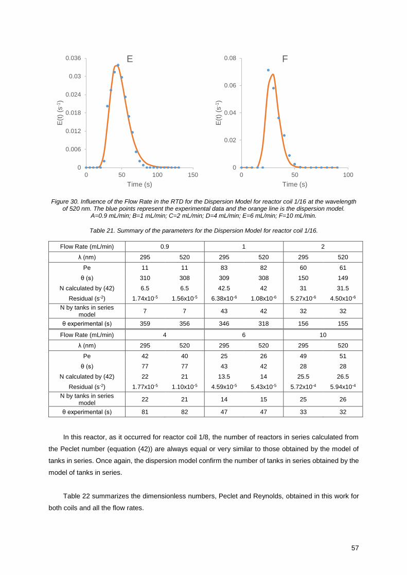
57
Figure 30. Influence of the Flow Rate in the RTD for the Dispersion Model for reactor coil 1/16 at the wavelength of 520 nm. The blue points represent the experimental data and the orange line is the dispersion model.
A=0.9 mL/min; B=1 mL/min; C=2 mL/min; D=4 mL/min; E=6 mL/min; F=10 mL/min.
Table 21. Summary of the parameters for the Dispersion Model for reactor coil 1/16.
In this reactor, as it occurred for reactor coil 1/8, the number of reactors in series calculated from
the Peclet number (equation (42)) are always equal or very similar to those obtained by the model of
tanks in series. Once again, the dispersion model confirm the number of tanks in series obtained by the
model of tanks in series.
Table 22 summarizes the dimensionless numbers, Peclet and Reynolds, obtained in this work for
both coils and all the flow rates.
0
0.006
0.012
0.018
0.024
0.03
0.036
0 50 100 150
E(t
)(s
-1)
Time (s)
E
0
0.02
0.04
0.06
0.08
0 50 100
E(t
)(s
-1)
Time (s)
F
Flow Rate (mL/min) 0.9 1 2
λ (nm) 295 520 295 520 295 520
Pe 11 11 83 82 60 61
θ (s) 310 308 309 308 150 149
N calculated by (42) 6.5 6.5 42.5 42 31 31.5
Residual (s-2) 1.74x10⁻⁵ 1.56x10⁻⁵ 6.38x10⁻⁶ 1.08x10⁻⁶ 5.27x10⁻⁶ 4.50x10⁻⁶
N by tanks in series model
7 7 43 42 32 32
θ experimental (s) 359 356 346 318 156 155
Flow Rate (mL/min) 4 6 10
λ (nm) 295 520 295 520 295 520
Pe 42 40 25 26 49 51
θ (s) 77 77 43 42 28 28
N calculated by (42) 22 21 13.5 14 25.5 26.5
Residual (s-2) 1.77x10⁻⁵ 1.10x10⁻⁵ 4.59x10⁻⁵ 5.43x10⁻⁵ 5.72x10⁻⁴ 5.94x10⁻⁴
N by tanks in series model
22 21 14 15 25 26
θ experimental (s) 81 82 47 47 33 32
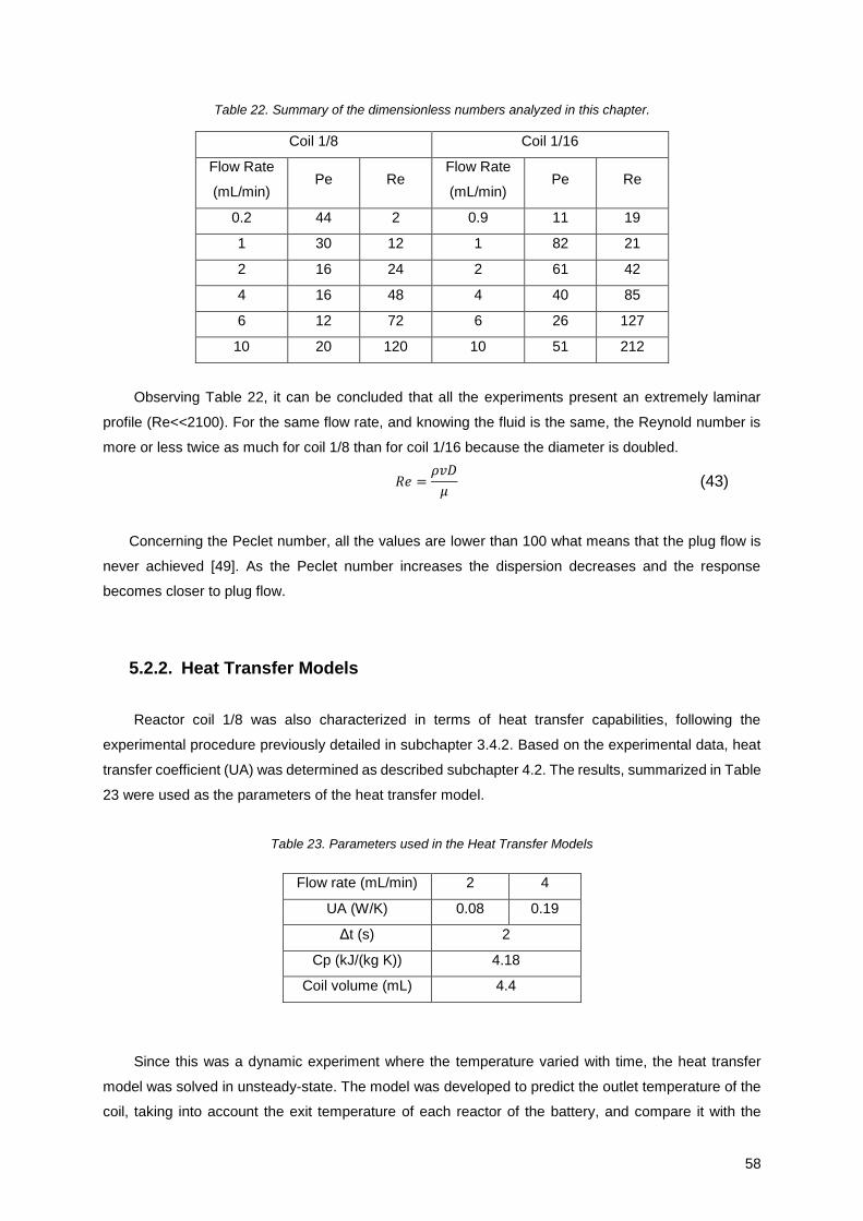
58
Table 22. Summary of the dimensionless numbers analyzed in this chapter.
Coil 1/8 Coil 1/16
Flow Rate
(mL/min) Pe Re
Flow Rate
(mL/min) Pe Re
0.2 44 2 0.9 11 19
1 30 12 1 82 21
2 16 24 2 61 42
4 16 48 4 40 85
6 12 72 6 26 127
10 20 120 10 51 212
Observing Table 22, it can be concluded that all the experiments present an extremely laminar
profile (Re<<2100). For the same flow rate, and knowing the fluid is the same, the Reynold number is
more or less twice as much for coil 1/8 than for coil 1/16 because the diameter is doubled.
𝑅𝑒 =𝜌𝑣𝐷
𝜇 (43)
Concerning the Peclet number, all the values are lower than 100 what means that the plug flow is
never achieved [49]. As the Peclet number increases the dispersion decreases and the response
becomes closer to plug flow.
5.2.2. Heat Transfer Models
Reactor coil 1/8 was also characterized in terms of heat transfer capabilities, following the
experimental procedure previously detailed in subchapter 3.4.2. Based on the experimental data, heat
transfer coefficient (UA) was determined as described subchapter 4.2. The results, summarized in Table
23 were used as the parameters of the heat transfer model.
Table 23. Parameters used in the Heat Transfer Models
Flow rate (mL/min) 2 4
UA (W/K) 0.08 0.19
Δt (s) 2
Cp (kJ/(kg K)) 4.18
Coil volume (mL) 4.4
Since this was a dynamic experiment where the temperature varied with time, the heat transfer
model was solved in unsteady-state. The model was developed to predict the outlet temperature of the
coil, taking into account the exit temperature of each reactor of the battery, and compare it with the
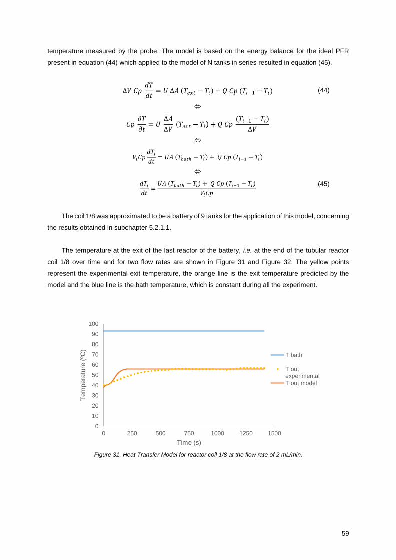
59
temperature measured by the probe. The model is based on the energy balance for the ideal PFR
present in equation (44) which applied to the model of N tanks in series resulted in equation (45).
∆𝑉 𝐶𝑝 𝑑𝑇
𝑑𝑡= 𝑈 ∆𝐴 (𝑇𝑒𝑥𝑡 − 𝑇𝑖) + 𝑄 𝐶𝑝 (𝑇𝑖−1 − 𝑇𝑖) (44)
𝐶𝑝 𝜕𝑇
𝜕𝑡= 𝑈
∆𝐴
∆𝑉 (𝑇𝑒𝑥𝑡 − 𝑇𝑖) + 𝑄 𝐶𝑝
(𝑇𝑖−1 − 𝑇𝑖)
∆𝑉
𝑉𝑖𝐶𝑝𝑑𝑇𝑖
𝑑𝑡= 𝑈𝐴 (𝑇𝑏𝑎𝑡ℎ − 𝑇𝑖) + 𝑄 𝐶𝑝 (𝑇𝑖−1 − 𝑇𝑖)
𝑑𝑇𝑖
𝑑𝑡=
𝑈𝐴 (𝑇𝑏𝑎𝑡ℎ − 𝑇𝑖) + 𝑄 𝐶𝑝 (𝑇𝑖−1 − 𝑇𝑖)
𝑉𝑖𝐶𝑝
(45)
The coil 1/8 was approximated to be a battery of 9 tanks for the application of this model, concerning
the results obtained in subchapter 5.2.1.1.
The temperature at the exit of the last reactor of the battery, i.e. at the end of the tubular reactor
coil 1/8 over time and for two flow rates are shown in Figure 31 and Figure 32. The yellow points
represent the experimental exit temperature, the orange line is the exit temperature predicted by the
model and the blue line is the bath temperature, which is constant during all the experiment.
Figure 31. Heat Transfer Model for reactor coil 1/8 at the flow rate of 2 mL/min.
0
10
20
30
40
50
60
70
80
90
100
0 250 500 750 1000 1250 1500
Tem
pera
ture
(ºC
)
Time (s)
T bath
T outexperimental
T out model
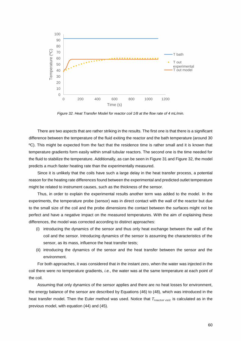
60
Figure 32. Heat Transfer Model for reactor coil 1/8 at the flow rate of 4 mL/min.
There are two aspects that are rather striking in the results. The first one is that there is a significant
difference between the temperature of the fluid exiting the reactor and the bath temperature (around 30
ºC). This might be expected from the fact that the residence time is rather small and it is known that
temperature gradients form easily within small tubular reactors. The second one is the time needed for
the fluid to stabilize the temperature. Additionally, as can be seen in Figure 31 and Figure 32, the model
predicts a much faster heating rate than the experimentally measured.
Since it is unlikely that the coils have such a large delay in the heat transfer process, a potential
reason for the heating rate differences found between the experimental and predicted outlet temperature
might be related to instrument causes, such as the thickness of the sensor.
Thus, in order to explain the experimental results another term was added to the model. In the
experiments, the temperature probe (sensor) was in direct contact with the wall of the reactor but due
to the small size of the coil and the probe dimensions the contact between the surfaces might not be
perfect and have a negative impact on the measured temperatures. With the aim of explaining these
differences, the model was corrected according to distinct approaches:
(i) introducing the dynamics of the sensor and thus only heat exchange between the wall of the
coil and the sensor. Introducing dynamics of the sensor is assuming the characteristics of the
sensor, as its mass, influence the heat transfer tests;
(ii) introducing the dynamics of the sensor and the heat transfer between the sensor and the
environment.
For both approaches, it was considered that in the instant zero, when the water was injected in the
coil there were no temperature gradients, i.e., the water was at the same temperature at each point of
the coil.
Assuming that only dynamics of the sensor applies and there are no heat losses for environment,
the energy balance of the sensor are described by Equations (46) to (48), which was introduced in the
heat transfer model. Then the Euler method was used. Notice that 𝑇𝑟𝑒𝑎𝑐𝑡𝑜𝑟 𝑒𝑥𝑖𝑡 is calculated as in the
previous model, with equation (44) and (45).
0
10
20
30
40
50
60
70
80
90
100
0 200 400 600 800 1000 1200
Tem
pera
ture
(ºC
)
Time (s)
T bath
T outexperimentalT out model
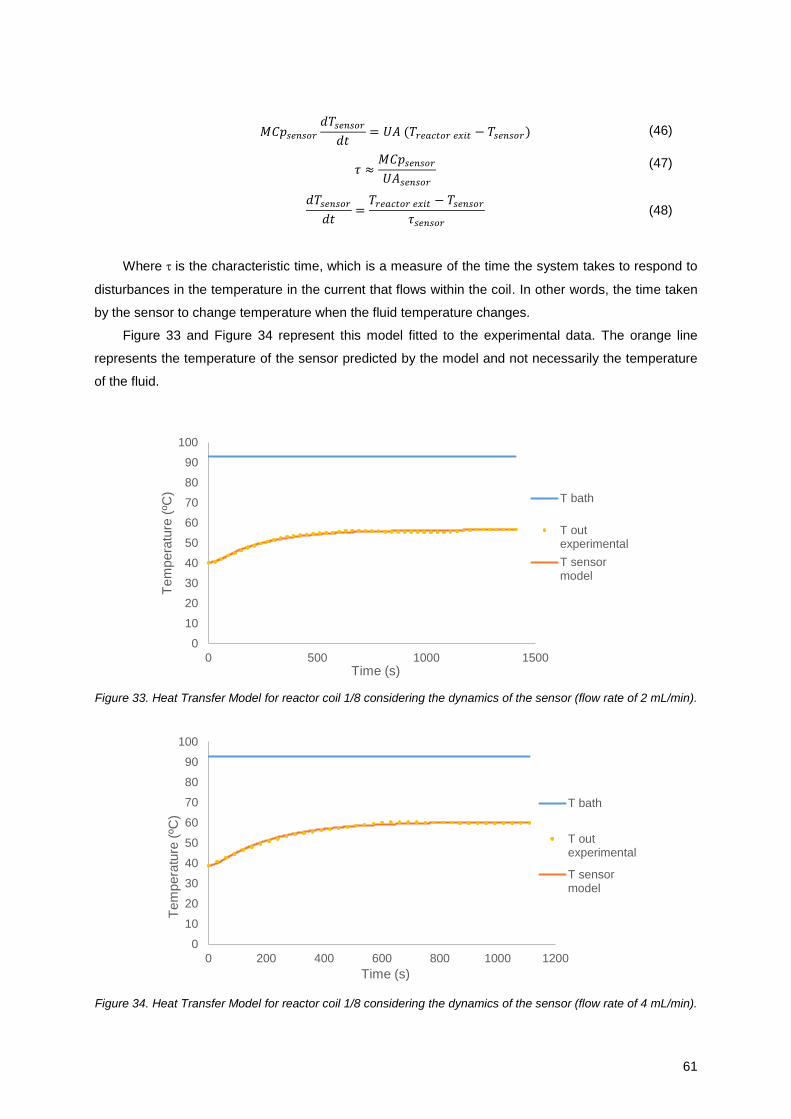
61
Where is the characteristic time, which is a measure of the time the system takes to respond to
disturbances in the temperature in the current that flows within the coil. In other words, the time taken
by the sensor to change temperature when the fluid temperature changes.
Figure 33 and Figure 34 represent this model fitted to the experimental data. The orange line
represents the temperature of the sensor predicted by the model and not necessarily the temperature
of the fluid.
Figure 33. Heat Transfer Model for reactor coil 1/8 considering the dynamics of the sensor (flow rate of 2 mL/min).
Figure 34. Heat Transfer Model for reactor coil 1/8 considering the dynamics of the sensor (flow rate of 4 mL/min).
0
10
20
30
40
50
60
70
80
90
100
0 500 1000 1500
Tem
pera
ture
(ºC
)
Time (s)
T bath
T outexperimental
T sensormodel
0
10
20
30
40
50
60
70
80
90
100
0 200 400 600 800 1000 1200
Tem
pera
ture
(ºC
)
Time (s)
T bath
T outexperimental
T sensormodel
𝑀𝐶𝑝𝑠𝑒𝑛𝑠𝑜𝑟
𝑑𝑇𝑠𝑒𝑛𝑠𝑜𝑟
𝑑𝑡= 𝑈𝐴 (𝑇𝑟𝑒𝑎𝑐𝑡𝑜𝑟 𝑒𝑥𝑖𝑡 − 𝑇𝑠𝑒𝑛𝑠𝑜𝑟) (46)
𝜏 ≈𝑀𝐶𝑝𝑠𝑒𝑛𝑠𝑜𝑟
𝑈𝐴𝑠𝑒𝑛𝑠𝑜𝑟
(47)
𝑑𝑇𝑠𝑒𝑛𝑠𝑜𝑟
𝑑𝑡=
𝑇𝑟𝑒𝑎𝑐𝑡𝑜𝑟 𝑒𝑥𝑖𝑡 − 𝑇𝑠𝑒𝑛𝑠𝑜𝑟
𝜏𝑠𝑒𝑛𝑠𝑜𝑟
(48)
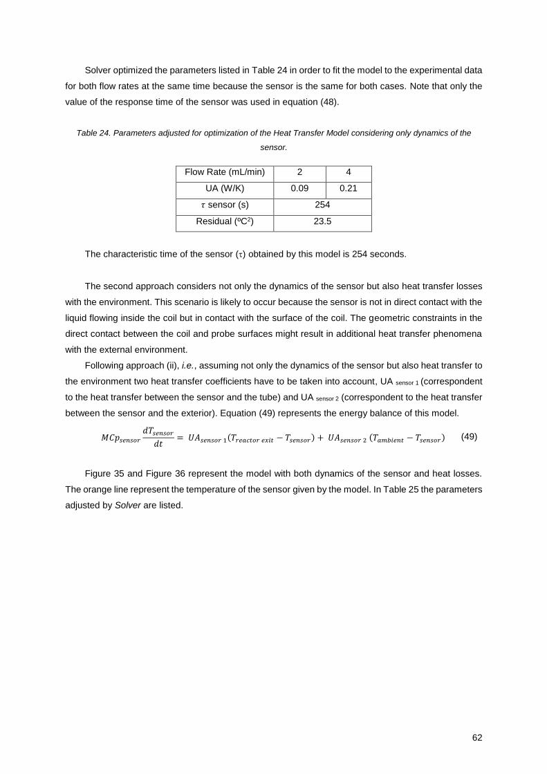
62
Solver optimized the parameters listed in Table 24 in order to fit the model to the experimental data
for both flow rates at the same time because the sensor is the same for both cases. Note that only the
value of the response time of the sensor was used in equation (48).
Table 24. Parameters adjusted for optimization of the Heat Transfer Model considering only dynamics of the
sensor.
Flow Rate (mL/min) 2 4
UA (W/K) 0.09 0.21
𝜏 sensor (s) 254
Residual (ºC2) 23.5
The characteristic time of the sensor () obtained by this model is 254 seconds.
The second approach considers not only the dynamics of the sensor but also heat transfer losses
with the environment. This scenario is likely to occur because the sensor is not in direct contact with the
liquid flowing inside the coil but in contact with the surface of the coil. The geometric constraints in the
direct contact between the coil and probe surfaces might result in additional heat transfer phenomena
with the external environment.
Following approach (ii), i.e., assuming not only the dynamics of the sensor but also heat transfer to
the environment two heat transfer coefficients have to be taken into account, UA sensor 1 (correspondent
to the heat transfer between the sensor and the tube) and UA sensor 2 (correspondent to the heat transfer
between the sensor and the exterior). Equation (49) represents the energy balance of this model.
Figure 35 and Figure 36 represent the model with both dynamics of the sensor and heat losses.
The orange line represent the temperature of the sensor given by the model. In Table 25 the parameters
adjusted by Solver are listed.
𝑀𝐶𝑝𝑠𝑒𝑛𝑠𝑜𝑟
𝑑𝑇𝑠𝑒𝑛𝑠𝑜𝑟
𝑑𝑡= 𝑈𝐴𝑠𝑒𝑛𝑠𝑜𝑟 1(𝑇𝑟𝑒𝑎𝑐𝑡𝑜𝑟 𝑒𝑥𝑖𝑡 − 𝑇𝑠𝑒𝑛𝑠𝑜𝑟) + 𝑈𝐴𝑠𝑒𝑛𝑠𝑜𝑟 2 (𝑇𝑎𝑚𝑏𝑖𝑒𝑛𝑡 − 𝑇𝑠𝑒𝑛𝑠𝑜𝑟) (49)
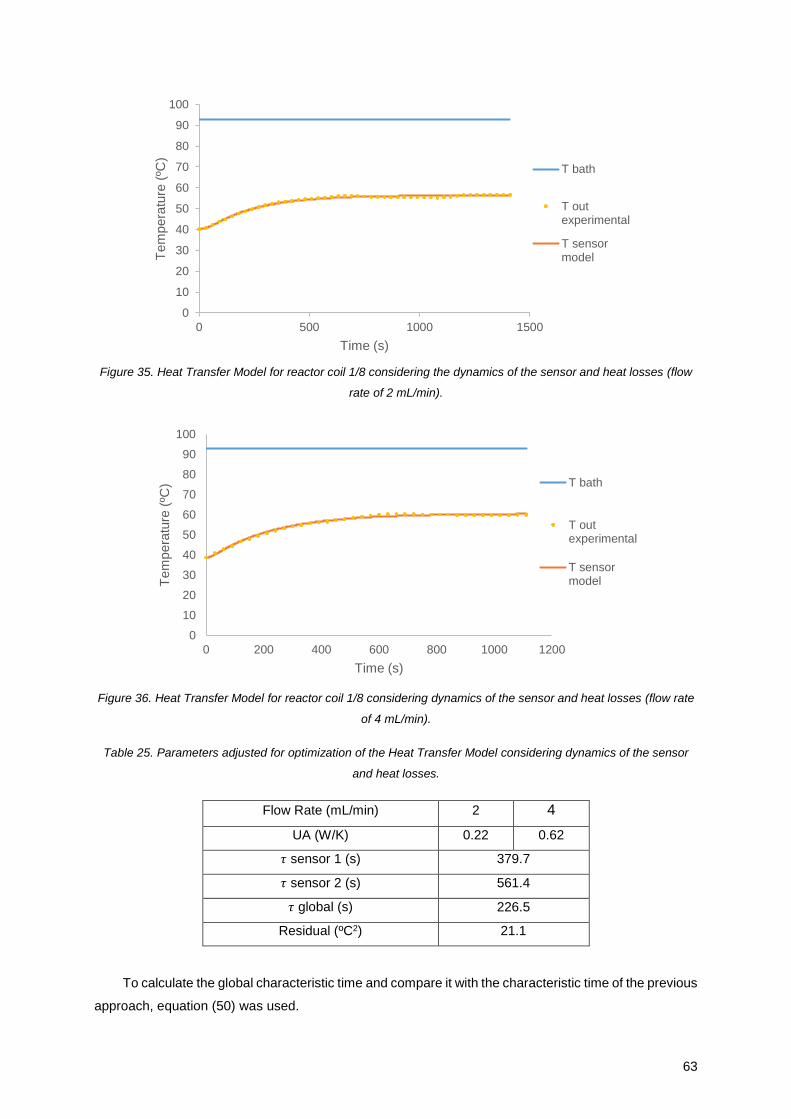
63
Figure 35. Heat Transfer Model for reactor coil 1/8 considering the dynamics of the sensor and heat losses (flow
rate of 2 mL/min).
Figure 36. Heat Transfer Model for reactor coil 1/8 considering dynamics of the sensor and heat losses (flow rate
of 4 mL/min).
Table 25. Parameters adjusted for optimization of the Heat Transfer Model considering dynamics of the sensor
and heat losses.
Flow Rate (mL/min) 2 4
UA (W/K) 0.22 0.62
𝜏 sensor 1 (s) 379.7
𝜏 sensor 2 (s) 561.4
𝜏 global (s) 226.5
Residual (ºC2) 21.1
To calculate the global characteristic time and compare it with the characteristic time of the previous
approach, equation (50) was used.
0
10
20
30
40
50
60
70
80
90
100
0 500 1000 1500
Tem
pera
ture
(ºC
)
Time (s)
T bath
T outexperimental
T sensormodel
0
10
20
30
40
50
60
70
80
90
100
0 200 400 600 800 1000 1200
Tem
pera
ture
(ºC
)
Time (s)
T bath
T outexperimental
T sensormodel
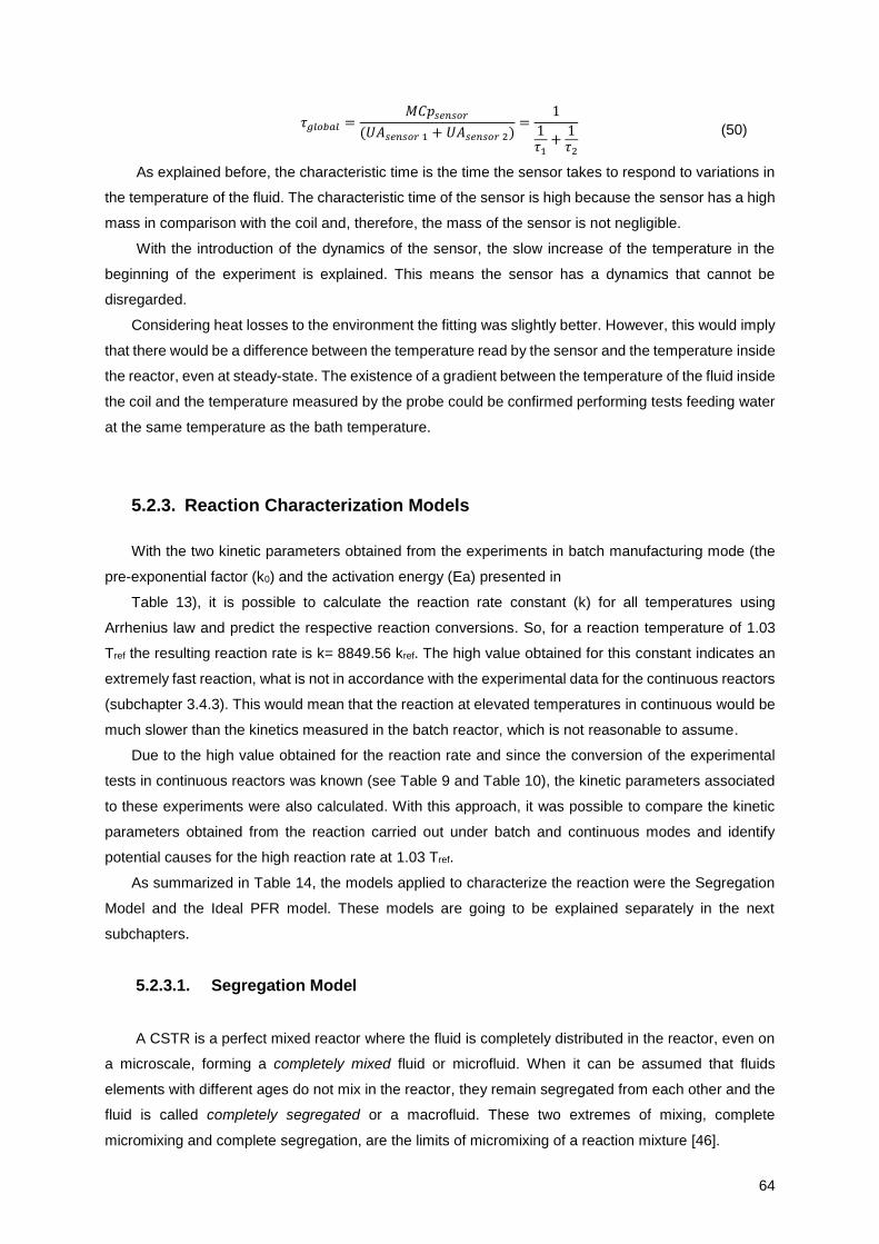
64
𝜏𝑔𝑙𝑜𝑏𝑎𝑙 =
𝑀𝐶𝑝𝑠𝑒𝑛𝑠𝑜𝑟
(𝑈𝐴𝑠𝑒𝑛𝑠𝑜𝑟 1 + 𝑈𝐴𝑠𝑒𝑛𝑠𝑜𝑟 2)=
1
1𝜏1
+1𝜏2
(50)
As explained before, the characteristic time is the time the sensor takes to respond to variations in
the temperature of the fluid. The characteristic time of the sensor is high because the sensor has a high
mass in comparison with the coil and, therefore, the mass of the sensor is not negligible.
With the introduction of the dynamics of the sensor, the slow increase of the temperature in the
beginning of the experiment is explained. This means the sensor has a dynamics that cannot be
disregarded.
Considering heat losses to the environment the fitting was slightly better. However, this would imply
that there would be a difference between the temperature read by the sensor and the temperature inside
the reactor, even at steady-state. The existence of a gradient between the temperature of the fluid inside
the coil and the temperature measured by the probe could be confirmed performing tests feeding water
at the same temperature as the bath temperature.
5.2.3. Reaction Characterization Models
With the two kinetic parameters obtained from the experiments in batch manufacturing mode (the
pre-exponential factor (k0) and the activation energy (Ea) presented in
Table 13), it is possible to calculate the reaction rate constant (k) for all temperatures using
Arrhenius law and predict the respective reaction conversions. So, for a reaction temperature of 1.03
Tref the resulting reaction rate is k= 8849.56 kref. The high value obtained for this constant indicates an
extremely fast reaction, what is not in accordance with the experimental data for the continuous reactors
(subchapter 3.4.3). This would mean that the reaction at elevated temperatures in continuous would be
much slower than the kinetics measured in the batch reactor, which is not reasonable to assume.
Due to the high value obtained for the reaction rate and since the conversion of the experimental
tests in continuous reactors was known (see Table 9 and Table 10), the kinetic parameters associated
to these experiments were also calculated. With this approach, it was possible to compare the kinetic
parameters obtained from the reaction carried out under batch and continuous modes and identify
potential causes for the high reaction rate at 1.03 Tref.
As summarized in Table 14, the models applied to characterize the reaction were the Segregation
Model and the Ideal PFR model. These models are going to be explained separately in the next
subchapters.
5.2.3.1. Segregation Model
A CSTR is a perfect mixed reactor where the fluid is completely distributed in the reactor, even on
a microscale, forming a completely mixed fluid or microfluid. When it can be assumed that fluids
elements with different ages do not mix in the reactor, they remain segregated from each other and the
fluid is called completely segregated or a macrofluid. These two extremes of mixing, complete
micromixing and complete segregation, are the limits of micromixing of a reaction mixture [46].
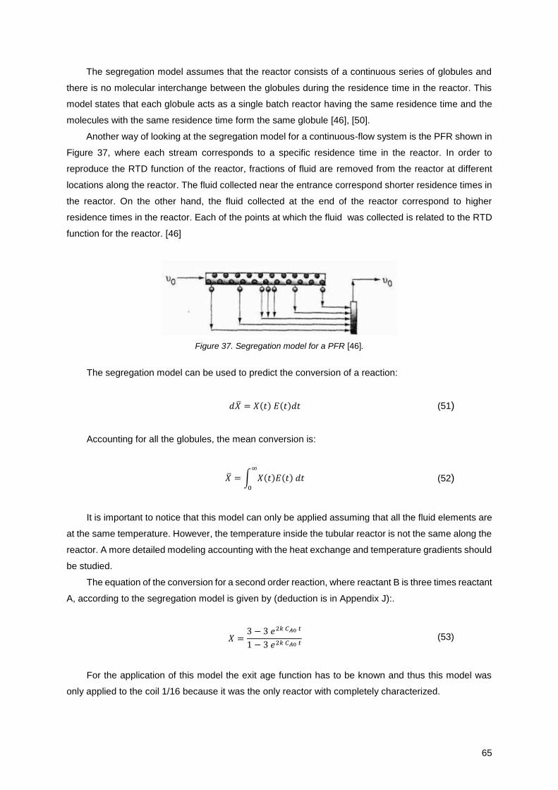
65
The segregation model assumes that the reactor consists of a continuous series of globules and
there is no molecular interchange between the globules during the residence time in the reactor. This
model states that each globule acts as a single batch reactor having the same residence time and the
molecules with the same residence time form the same globule [46], [50].
Another way of looking at the segregation model for a continuous-flow system is the PFR shown in
Figure 37, where each stream corresponds to a specific residence time in the reactor. In order to
reproduce the RTD function of the reactor, fractions of fluid are removed from the reactor at different
locations along the reactor. The fluid collected near the entrance correspond shorter residence times in
the reactor. On the other hand, the fluid collected at the end of the reactor correspond to higher
residence times in the reactor. Each of the points at which the fluid was collected is related to the RTD
function for the reactor. [46]
Figure 37. Segregation model for a PFR [46].
The segregation model can be used to predict the conversion of a reaction:
𝑑�̅� = 𝑋(𝑡) 𝐸(𝑡)𝑑𝑡 (51)
Accounting for all the globules, the mean conversion is:
�̅� = ∫ 𝑋(𝑡)𝐸(𝑡) 𝑑𝑡∞
0
(52)
It is important to notice that this model can only be applied assuming that all the fluid elements are
at the same temperature. However, the temperature inside the tubular reactor is not the same along the
reactor. A more detailed modeling accounting with the heat exchange and temperature gradients should
be studied.
The equation of the conversion for a second order reaction, where reactant B is three times reactant
A, according to the segregation model is given by (deduction is in Appendix J):.
𝑋 =3 − 3 𝑒2𝑘 𝐶𝐴0 𝑡
1 − 3 𝑒2𝑘 𝐶𝐴0 𝑡 (53)
For the application of this model the exit age function has to be known and thus this model was
only applied to the coil 1/16 because it was the only reactor with completely characterized.
66
The model of two batteries in parallel was used in order to obtain an expression of E(t) and being
in the conditions of using the equation (52). More specifically, the model adjusted for all the flow rates
was chosen, whose parameters are listed in Table 19.
The residence times used in the continuous experiments (Table 9) were introduced in the
expression of E(t) (equation (38)) so that the conversion could be compared because for those residence
times the conversion was obtained experimentally.
The equation (53) depends on the reaction rate constant, k, and the initial concentration of reactant
A. The concentration of A is known, so the only parameter unknown is k. As three temperatures 1.03,
1.05 and 1.08 Tref were tested in the experiments, the activation energy, Ea, was also calculated. Solver
adjusted these two kinetic parameters (k and Ea) with the aim of obtaining a conversion as close to the
experimental conversion as possible. It is important to note that the interval between the three
temperatures used was very small to estimate activation energies and, therefore, estimation might be
affected with some error. In fact, the value obtained for the activation energy was very low. Table 26
presents the kinetic parameters obtained. R2 is a measure of adjustment between the experimental
values and the values calculated by the model.
Figure 38 represents the experimental conversion and the conversion obtained from the model.
Figure 38. Experimental and calculated conversion by the Segregation Model for reactor coil 1/16.
Table 26. Kinetic parameters obtained from the Segregation Model for reactor coil 1/16.
k1.03 Tref 9.03 kref
Ea 0.22 Earef
R2 0.809
5.2.3.2. Ideal PFR Model
The Ideal Plug Flow Reactor (PFR) model is a model used to describe the performance of
continuous reactors, which assume complete radial mixing but no mixing in the axial direction.
0.0
0.4
0.8
1.2
1.6
2.0
0 5 10 15 20 25
% H
PLC
/ %
HP
LC
ref
Residence Time (min)
conversioncalculated
conversionobtainedexperimentally
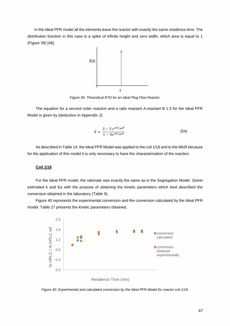
67
In the Ideal PFR model all the elements leave the reactor with exactly the same residence time. The
distribution function in this case is a spike of infinite height and zero width, which area is equal to 1
(Figure 39) [46].
Figure 39. Theoretical RTD for an Ideal Plug Flow Reactor.
The equation for a second order reaction and a ratio reactant A:reactant B 1:3 for the Ideal PFR
Model is given by (deduction in Appendix J):
𝑋 = 3 − 3 𝑒2𝑘𝐶𝐴0𝜃
1 − 3𝑒2𝑘𝐶𝐴0𝜃 (54)
As described in Table 14, the Ideal PFR Model was applied to the coil 1/16 and to the MicR because
for the application of this model it is only necessary to have the characterization of the reaction.
Coil 1/16
For the Ideal PFR model, the rationale was exactly the same as in the Segregation Model. Solver
estimated k and Ea with the purpose of obtaining the kinetic parameters which best described the
conversion obtained in the laboratory (Table 9).
Figure 40 represents the experimental conversion and the conversion calculated by the Ideal PFR
model. Table 27 presents the kinetic parameters obtained.
Figure 40. Experimental and calculated conversion by the Ideal PFR Model for reactor coil 1/16.
0.0
0.4
0.8
1.2
1.6
2.0
0 5 10 15 20 25
% H
PL
C / %
HP
LC
re
f
Residence Time (min)
conversioncalculated
conversionobtainedexperimentally
68
Table 27. Kinetic parameters obtained from the Ideal PFR Model for reactor coil 1/16.
k1.03 Tref 11.33 kref
Ea 0.09 Earef
R2 0.905
According to the results summarized in Table 26 and Table 27, it can be concluded that both models
give identical results for the kinetic parameters. Besides the activation energy obtained from the two
models is not as similar as the rate constant, the values are in the same order of magnitude.
MicR
Although there was not performed characterization tests for the reactor MicR, the kinetic parameters
of reaction were also estimated by the Ideal PFR Model. Thus, the same methodology was followed as
in the reactor coil 1/16. Solver estimated k and Ea with the aim of obtaining the kinetic parameters which
best described the conversion obtained in the laboratory (Table 10).
Figure 41 represents the experimental conversion and the conversion calculated by the Ideal PFR
model. Table 28 presents the kinetic parameters obtained.
Figure 41. Experimental and calculated conversion by the Ideal PFR Model for reactor MicR.
Table 28. Kinetic parameters obtained from the Ideal PFR Model for reactor MicR.
k1.03 Tref 7.67 kref
Ea 0.44 Earef
R2 0.996
In Figure 41, three of the residence times have two conversions for two different temperatures (0.82
Tref and Tref) and the conversion for each temperature was calculated. The kinetic parameters obtained
for the micro-reactor are consistent with those obtained for the coil reactor. Activation energy is the
variable that shows higher differences depending on the model applied. One reason for this is the small
interval of temperatures for the estimation of it.
0.0
0.4
0.8
1.2
1.6
2.0
0 5 10 15 20
% H
PL
C / %
HP
LC
re
f
Residence Time (min)
conversioncalculated
conversionobtainedexperimentally
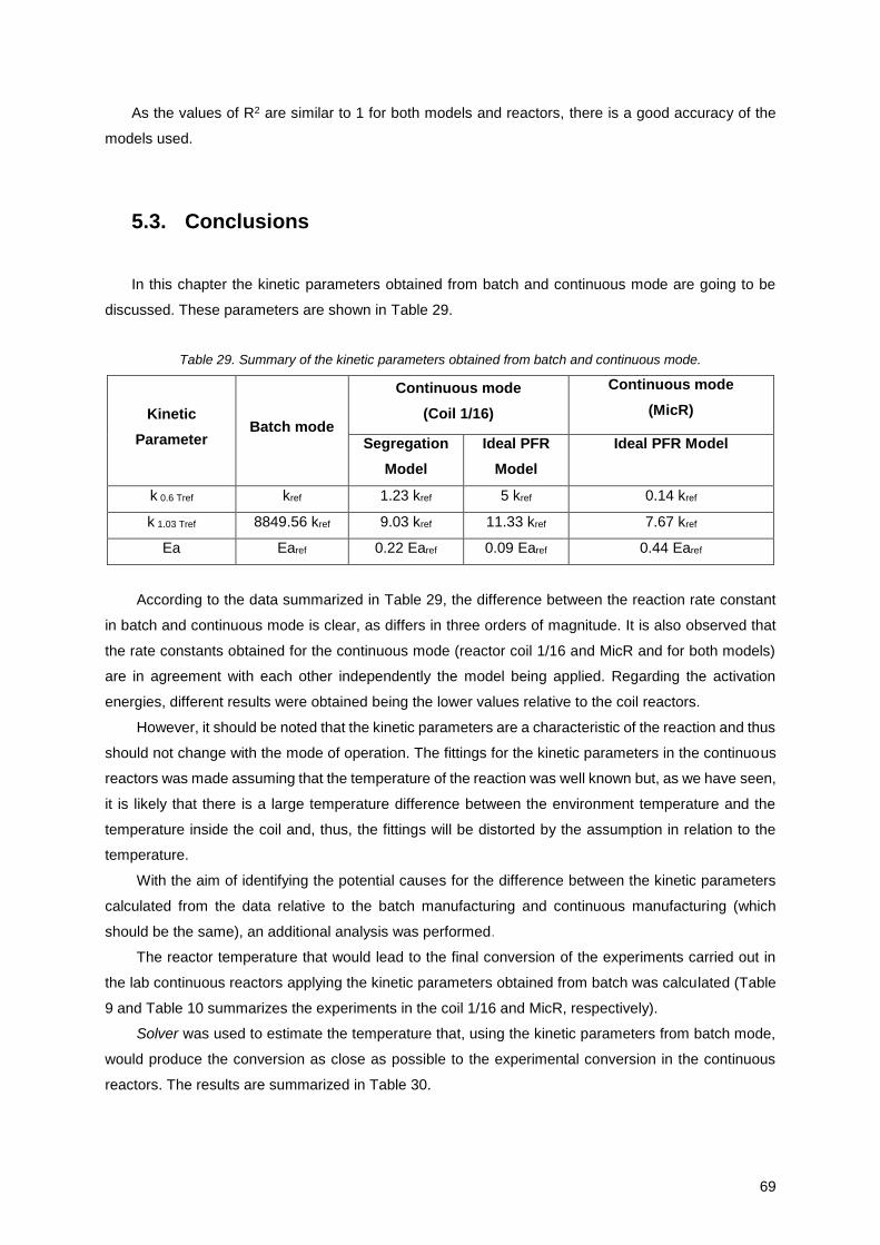
69
As the values of R2 are similar to 1 for both models and reactors, there is a good accuracy of the
models used.
5.3. Conclusions
In this chapter the kinetic parameters obtained from batch and continuous mode are going to be
discussed. These parameters are shown in Table 29.
Table 29. Summary of the kinetic parameters obtained from batch and continuous mode.
Kinetic
Parameter Batch mode
Continuous mode
(Coil 1/16)
Continuous mode
(MicR)
Segregation
Model
Ideal PFR
Model
Ideal PFR Model
k 0.6 Tref kref 1.23 kref 5 kref 0.14 kref
k 1.03 Tref 8849.56 kref 9.03 kref 11.33 kref 7.67 kref
Ea Earef 0.22 Earef 0.09 Earef 0.44 Earef
According to the data summarized in Table 29, the difference between the reaction rate constant
in batch and continuous mode is clear, as differs in three orders of magnitude. It is also observed that
the rate constants obtained for the continuous mode (reactor coil 1/16 and MicR and for both models)
are in agreement with each other independently the model being applied. Regarding the activation
energies, different results were obtained being the lower values relative to the coil reactors.
However, it should be noted that the kinetic parameters are a characteristic of the reaction and thus
should not change with the mode of operation. The fittings for the kinetic parameters in the continuous
reactors was made assuming that the temperature of the reaction was well known but, as we have seen,
it is likely that there is a large temperature difference between the environment temperature and the
temperature inside the coil and, thus, the fittings will be distorted by the assumption in relation to the
temperature.
With the aim of identifying the potential causes for the difference between the kinetic parameters
calculated from the data relative to the batch manufacturing and continuous manufacturing (which
should be the same), an additional analysis was performed.
The reactor temperature that would lead to the final conversion of the experiments carried out in
the lab continuous reactors applying the kinetic parameters obtained from batch was calculated (Table
9 and Table 10 summarizes the experiments in the coil 1/16 and MicR, respectively).
Solver was used to estimate the temperature that, using the kinetic parameters from batch mode,
would produce the conversion as close as possible to the experimental conversion in the continuous
reactors. The results are summarized in Table 30.
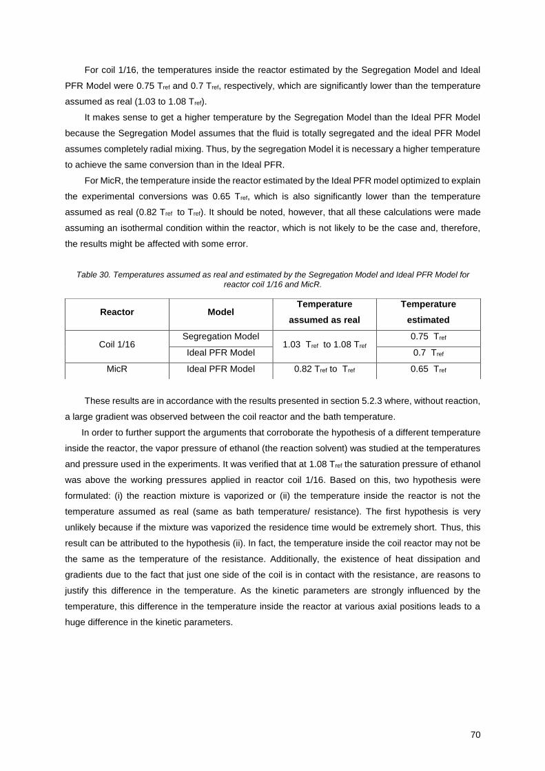
70
For coil 1/16, the temperatures inside the reactor estimated by the Segregation Model and Ideal
PFR Model were 0.75 Tref and 0.7 Tref, respectively, which are significantly lower than the temperature
assumed as real (1.03 to 1.08 Tref).
It makes sense to get a higher temperature by the Segregation Model than the Ideal PFR Model
because the Segregation Model assumes that the fluid is totally segregated and the ideal PFR Model
assumes completely radial mixing. Thus, by the segregation Model it is necessary a higher temperature
to achieve the same conversion than in the Ideal PFR.
For MicR, the temperature inside the reactor estimated by the Ideal PFR model optimized to explain
the experimental conversions was 0.65 Tref, which is also significantly lower than the temperature
assumed as real (0.82 Tref to Tref). It should be noted, however, that all these calculations were made
assuming an isothermal condition within the reactor, which is not likely to be the case and, therefore,
the results might be affected with some error.
Table 30. Temperatures assumed as real and estimated by the Segregation Model and Ideal PFR Model for
reactor coil 1/16 and MicR.
These results are in accordance with the results presented in section 5.2.3 where, without reaction,
a large gradient was observed between the coil reactor and the bath temperature.
In order to further support the arguments that corroborate the hypothesis of a different temperature
inside the reactor, the vapor pressure of ethanol (the reaction solvent) was studied at the temperatures
and pressure used in the experiments. It was verified that at 1.08 Tref the saturation pressure of ethanol
was above the working pressures applied in reactor coil 1/16. Based on this, two hypothesis were
formulated: (i) the reaction mixture is vaporized or (ii) the temperature inside the reactor is not the
temperature assumed as real (same as bath temperature/ resistance). The first hypothesis is very
unlikely because if the mixture was vaporized the residence time would be extremely short. Thus, this
result can be attributed to the hypothesis (ii). In fact, the temperature inside the coil reactor may not be
the same as the temperature of the resistance. Additionally, the existence of heat dissipation and
gradients due to the fact that just one side of the coil is in contact with the resistance, are reasons to
justify this difference in the temperature. As the kinetic parameters are strongly influenced by the
temperature, this difference in the temperature inside the reactor at various axial positions leads to a
huge difference in the kinetic parameters.
Reactor Model Temperature
assumed as real
Temperature
estimated
Coil 1/16 Segregation Model
1.03 Tref to 1.08 Tref 0.75 Tref
Ideal PFR Model 0.7 Tref
MicR Ideal PFR Model 0.82 Tref to Tref 0.65 Tref
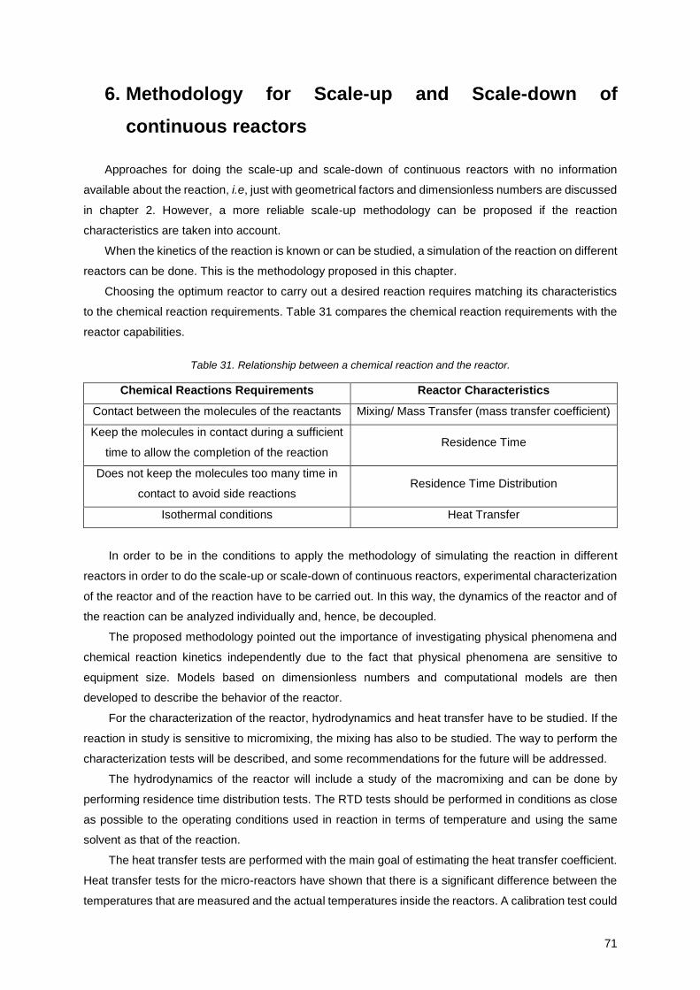
71
6. Methodology for Scale-up and Scale-down of
continuous reactors
Approaches for doing the scale-up and scale-down of continuous reactors with no information
available about the reaction, i.e, just with geometrical factors and dimensionless numbers are discussed
in chapter 2. However, a more reliable scale-up methodology can be proposed if the reaction
characteristics are taken into account.
When the kinetics of the reaction is known or can be studied, a simulation of the reaction on different
reactors can be done. This is the methodology proposed in this chapter.
Choosing the optimum reactor to carry out a desired reaction requires matching its characteristics
to the chemical reaction requirements. Table 31 compares the chemical reaction requirements with the
reactor capabilities.
Table 31. Relationship between a chemical reaction and the reactor.
Chemical Reactions Requirements Reactor Characteristics
Contact between the molecules of the reactants Mixing/ Mass Transfer (mass transfer coefficient)
Keep the molecules in contact during a sufficient
time to allow the completion of the reaction Residence Time
Does not keep the molecules too many time in
contact to avoid side reactions Residence Time Distribution
Isothermal conditions Heat Transfer
In order to be in the conditions to apply the methodology of simulating the reaction in different
reactors in order to do the scale-up or scale-down of continuous reactors, experimental characterization
of the reactor and of the reaction have to be carried out. In this way, the dynamics of the reactor and of
the reaction can be analyzed individually and, hence, be decoupled.
The proposed methodology pointed out the importance of investigating physical phenomena and
chemical reaction kinetics independently due to the fact that physical phenomena are sensitive to
equipment size. Models based on dimensionless numbers and computational models are then
developed to describe the behavior of the reactor.
For the characterization of the reactor, hydrodynamics and heat transfer have to be studied. If the
reaction in study is sensitive to micromixing, the mixing has also to be studied. The way to perform the
characterization tests will be described, and some recommendations for the future will be addressed.
The hydrodynamics of the reactor will include a study of the macromixing and can be done by
performing residence time distribution tests. The RTD tests should be performed in conditions as close
as possible to the operating conditions used in reaction in terms of temperature and using the same
solvent as that of the reaction.
The heat transfer tests are performed with the main goal of estimating the heat transfer coefficient.
Heat transfer tests for the micro-reactors have shown that there is a significant difference between the
temperatures that are measured and the actual temperatures inside the reactors. A calibration test could
72
be done to establish the temperature difference between what is being read by the probe and the actual
exit temperature of the reactor. One possibility would be to feed the reactor with a solution at the same
temperature as that of the bath or heating resistance so that no gradient exists between the heating
system and the reactor and so the outlet temperature is exactly known. In this case the sensor should
read at the exit of the reactor the same temperature as the bath. Since there is no gradient of
temperature between the bath/resistance and the fluid inside the reactor everything should be at the
same temperature. In this way, the difference between what the sensor is reading and the reactor exit
temperature can be estimated and an idea of the real temperature inside the reactor can be obtained
just by using the probe temperature.
As the calibration test only gives information about the exit temperature, a suggestion to gain more
insight into the temperature profile inside the continuous reactor is to carry out model reactions in those
reactors. A reaction with a well-known kinetics will have to be chosen. Ideally a simple reaction should
be used, which would be insensitive to micromixing effects. Examples of reactions that can be used are
the hydrolysis of methyl acetate and the iodation of acetone. The experimental determination of reaction
rates involves measuring how the concentrations of reactants or products change over time. With the
model of the reactor and the temperatures at the entrance and exit, the temperature profile inside the
reactor can be estimated and consequently the average temperature. In a tubular reactor the
temperature changes over the reactor, the fluid enters cold and takes time to heat. A slow or fast
temperature increase has a large impact on the average temperature inside the reactor.
Concerning the mixing and mass transfer studies, the caracterization of micromixing can be
performed using the Villermaux-Dushman reaction or any other reaction with non-linear kinetics (for
example second order reactions), since it is sensitive to micromixing [51].
As far as the characterization of the reaction is concerned, the thermodynamics and the kinetics of
the reaction have to be studied.
The thermodynamics of the reaction is important to study in order to know the equilibrium
conversion that can be achieve under specified conditions. The majority of highly exothermic reactions
are mostly displaced towards the products side so that they can be considered as irreversible. However,
it is important also to note that in exothermic reactions, higher temperatures displace the equilibrium for
the reagents side and for this reason the thermodynamic equilibrium has to be studied to know what is
the adequate temperature and pressure range.
Regarding the reaction kinetics, there are different ways to study it. Two possibilities will be using
a batch reactor or a continuous reactor. The typical approach is to study the kinetics in a batch reactor.
In batch, as it is necessary to collect samples and analyze, the sample properties can change in
that period of time. The advantage of studying the reaction kinetics in continuous is that when the steady
state in achieved the reaction is virtually “stopped” at specific conditions and, thus, the conditions of the
sample are well known and do not change. The disadvantages of studying the reaction kinetics in the
flow reactors are that geometry may be very different to that of the production scale and because it
might be more difficult to control and know exactly the operation conditions when compared to batch
mode, in particular due to the possibility of the occurrence of temperature gradients inside the reactor.
As analyzed before, it is very difficult to know exactly the temperature inside the continuous micro-
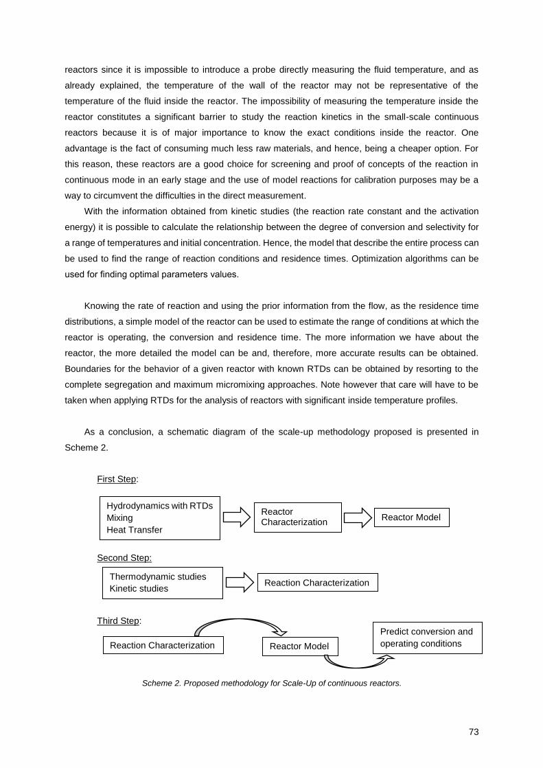
73
reactors since it is impossible to introduce a probe directly measuring the fluid temperature, and as
already explained, the temperature of the wall of the reactor may not be representative of the
temperature of the fluid inside the reactor. The impossibility of measuring the temperature inside the
reactor constitutes a significant barrier to study the reaction kinetics in the small-scale continuous
reactors because it is of major importance to know the exact conditions inside the reactor. One
advantage is the fact of consuming much less raw materials, and hence, being a cheaper option. For
this reason, these reactors are a good choice for screening and proof of concepts of the reaction in
continuous mode in an early stage and the use of model reactions for calibration purposes may be a
way to circumvent the difficulties in the direct measurement.
With the information obtained from kinetic studies (the reaction rate constant and the activation
energy) it is possible to calculate the relationship between the degree of conversion and selectivity for
a range of temperatures and initial concentration. Hence, the model that describe the entire process can
be used to find the range of reaction conditions and residence times. Optimization algorithms can be
used for finding optimal parameters values.
Knowing the rate of reaction and using the prior information from the flow, as the residence time
distributions, a simple model of the reactor can be used to estimate the range of conditions at which the
reactor is operating, the conversion and residence time. The more information we have about the
reactor, the more detailed the model can be and, therefore, more accurate results can be obtained.
Boundaries for the behavior of a given reactor with known RTDs can be obtained by resorting to the
complete segregation and maximum micromixing approaches. Note however that care will have to be
taken when applying RTDs for the analysis of reactors with significant inside temperature profiles.
As a conclusion, a schematic diagram of the scale-up methodology proposed is presented in
Scheme 2.
First Step:
Second Step:
Third Step:
Scheme 2. Proposed methodology for Scale-Up of continuous reactors.
Hydrodynamics with RTDs
Mixing
Heat Transfer
Reactor Characterization
Thermodynamic studies
Kinetic studies Reaction Characterization
Reaction Characterization Reactor Model
Predict conversion and
operating conditions
Reactor Model
74
7. Conclusions and Future Work
With the aim of developing a scale-up methodology for continuous processes, two tubular reactors
(coil 1/8 and coil 1/16) and one micro-reactor (MicR) were characterized and the reaction kinetics of a
case-study were analyzed.
There are different areas that have to be considered in terms of characterization of the reactors.
The first thing that has to be clearly characterized is the flow characteristics. The residence time
distribution measurements have shown that the continuous laboratory reactors studied have a complex
flow pattern that depends significantly on the total flow rate. The model of tanks in series, the model of
two batteries in parallel and the dispersion model were applied to the RTDs. The model that best
described the results obtained was the model of two batteries in parallel. A global fitting was tried with
this model in order to get a function that described the reactor independently on the flow rate, but as it
was concluded that the model described better the higher flow rates than the lower ones, other models
should be explored.
The reactors were further characterized in terms of heat transfer capabilities by carrying out heat
transfer tests. A better fitting to the reactor temperature profile was obtained, after introducing dynamics
of the sensor and heat losses between the sensor and the exterior. Nevertheless, a significant difference
between the temperature exiting the reactor and the bath temperature was observed.
In what concerns the characterization of the reaction, the kinetics of the reaction in batch operating
mode was studied, based on the mass and energy balances. As kinetic the parameters obtained were
not in accordance with the data for the reaction performed in the continuous reactors, the reaction
kinetics in continuous mode was also studied. Unexpected differences were found between the kinetic
parameters obtained from the two modes of operation. The reaction rate constant (k) at 1.03 Tref ranged
from 8849.56 kref in batch mode to 7.67 kref to 11.33 kref in continuous mode (coil 1/16 and MicR) applying
the Segregation and Ideal PFR Models. In order to explain this difference, the reactor temperature that
would lead to the final conversion of the experiments carried out in the continuous reactors applying the
kinetic parameters obtained from batch was calculated. It was concluded that the real temperature inside
the coil 1/16 and MicR was lower than the assumed temperature (1.03 Tref to 1.08 Tref, considered equal
to the resistance/bath temperature set point), ranging from 0.6 Tref to 0.75 Tref applying the before
mentioned models. Hence, it was concluded that significant differences exist in micro-reactors between
the heating resistance/bath temperature and the interior of the reactor.
As a conclusion, the dynamics of the reaction and of the reactor can be effectively decoupled if a
set of characterization tests are performed and if adequate calibrations can be done. Considering this,
a scale-up methodology was developed which is based on coupling the reaction information to a specific
reactor. A range of conditions at which the reactor might operate, conversion and residence time can
be estimated by a simple model of the reactor.
In order to achieve this goal some suggestions were made for future studies. By doing this, we will
be able to scale-up and scale-down continuous reactors or move from one reactor type to another in a
more effective way because a simulation of the reaction in distinct reactors is possible.
75
8. References
[1] T. LaPorte, C. Wang, and S. Jones, “Process Development and Case Studies of Continuous
Reactor Systems for Production of API and Pharmaceutical Intermediates,” in Chemical
Engineering in the Pharmaceutical Industry: R&D to Manufacturing, New Brunswick, NJ, USA,
2011, pp. 437–455.
[2] S. L. Lee et al., “Modernizing Pharmaceutical Manufacturing: from Batch to Continuous
Production,” J. Pharm. Innov., vol. 10, no. 3, pp. 191–199, 2015.
[3] FDA, “Modernizing the Way Drugs Are Made: A Transition to Continuous Manufacturing.”
[Online]. Available: https://www.fda.gov/Drugs/NewsEvents/ucm557448.htm. [Accessed: 07-Jul-
2017].
[4] A. Adamo et al., “On-demand continuous-flow production of pharmaceuticals in a compact,
reconfigurable system,” Science (80-. )., vol. 352, no. 6281, pp. 61–67, 2016.
[5] L. S. Ferreira and J. O. Trierweiler, “Modeling and simulation of the polymeric nanocapsule
formation process,” IFAC Proc. Vol., vol. 7, no. PART 1, pp. 405–410, 2009.
[6] R. L. Hartman, J. P. Mcmullen, and K. F. Jensen, “Flow Chemistry Deciding Whether To Go with
the Flow : Evaluating the Merits of Flow Reactors for Synthesis Angewandte,” pp. 7502–7519,
2011.
[7] F. Voice, “Continuous Manufacturing Has a Strong Impact on Drug Quality.” [Online]. Available:
https://blogs.fda.gov/fdavoice/index.php/2016/04/continuous-manufacturing-has-a-strong-
impact-on-drug-quality/. [Accessed: 05-Aug-2017].
[8] “The Benefits of Continuous Manufacturing,” Pharmaceutical Processing. [Online]. Available:
https://www.pharmpro.com/article/2016/12/benefits-continuous-manufacturing. [Accessed: 05-
May-2017].
[9] M. Baumann and I. R. Baxendale, “The synthesis of active pharmaceutical ingredients ( APIs )
using continuous flow chemistry,” pp. 1194–1219, 2015.
[10] J. Hartwig, J. B. Metternich, N. Nikbin, A. Kirschning, and S. V Ley, “Continuous flow chemistry:
a discovery tool for new chemical reactivity patterns.,” Org. Biomol. Chem., vol. 12, no. 22, pp.
3611–5, 2014.
[11] C. Wiles, “From Batch to Flow: Making the Switch,” Chemtrix, no. 2, 2009.
[12] G. de Maria, “IV Symposium on Continuous Flow Reactor Technology for Industrial Applications.”
[Online]. Available: http://www.teknoscienze.com/tks_article/4th-symposium-on-continuous-
flow-reactor-technology-for-industrial-applications/. [Accessed: 03-May-2017].
[13] P. Watts and C. Wiles, “Micro reactors, flow reactors and continuous flow synthesis,” J. Chem.
Res., vol. 36, no. 4, pp. 181–193, 2012.
[14] J. Wegner, S. Ceylan, and A. Kirschning, “Ten key issues in modern flow chemistry.,” Chem.
Commun. (Camb)., vol. 47, no. 16, pp. 4583–92, 2011.
[15] M. S. Croughan, K. B. Konstantinov, and C. Cooney, “The future of industrial bioprocessing:
Batch or continuous?,” Biotechnol. Bioeng., vol. 112, no. 4, pp. 648–651, 2015.
[16] “Visual Encyclopedia of Chemical Engineering,” College Engineering Chemical Engineering
University of Michigan. [Online]. Available:
76
http://encyclopedia.che.engin.umich.edu/Pages/Reactors/PFR/PFR.html. [Accessed: 23-Sep-
2017].
[17] W. L. Luyben, Chemical Reactor Design and Control. John Wiley & Sons, Inc, 2007.
[18] “Plug Flow Reactors (PFRs),” College Engineering Chemical Engineering University of Michigan.
[Online]. Available: http://umich.edu/~elements/asyLearn/bits/pfrfinal/index.htm. [Accessed: 23-
Sep-2017].
[19] C. R. Design, “Salamander Continuous Reactor Technology. The cost effective way to bring
Continuous Chemistry to every lab!” [Online]. Available:
http://www.cambridgereactordesign.com/pdf/Salamander A5 4pp v3.pdf. [Accessed: 10-Apr-
2017].
[20] C. R. Design, “Specifications. Salamander Jacketed Reactor with Capillary Tubing.” [Online].
Available: http://www.cambridgereactordesign.com/pdf/Salamader Jacketed Reactor with
Capillary Tubing. Specification.pdf. [Accessed: 10-Apr-2017].
[21] C. R. Design, “Specifications. Salamander Jacketed Reactor with Static Mixers.” [Online].
Available: http://www.cambridgereactordesign.com/pdf/Salamander Jacketed Reactor with
Static Mixers. A2_R0. Specification.pdf. [Accessed: 10-Apr-2017].
[22] P. I. Company, “Tubular Reactos Systems.” [Online]. Available: http://www.parrinst.com/wp-
content/uploads/downloads/2016/05/5400MB_Parr_Tubular-Reactor-Systems-Literature.pdf.
[Accessed: 10-Apr-2017].
[23] J. Yoshida, Y. Takahashi, and A. Nagaki, “Flash chemistry: flow chemistry that cannot be done
in batch.,” Chem. Commun. (Camb)., vol. 49, no. 85, pp. 9896–904, 2013.
[24] D. M. Roberge, M. Gottsponer, M. Eyholzer, and N. Kockmann, “Industrial design, scale-up, and
use of microreactors,” Chim. Oggi, vol. 27, no. 4, pp. 8–11, 2009.
[25] B. Gutmann, D. Cantillo, and C. O. Kappe, “Continuous-flow technology - A tool for the safe
manufacturing of active pharmaceutical ingredients,” Angew. Chemie, vol. 54, no. 23, pp. 6688–
6728, 2015.
[26] R. Reintjens, D. J. Ager, and A. H. M. De Vries, “Flow chemistry, how to bring it to industrial
scale?,” Chim. Oggi/Chemistry Today, vol. 33, no. 4, pp. 21–24, 2015.
[27] “Microreactor Concept Powering Your Innovation,” Lonza. [Online]. Available:
http://bio.lonza.com/uploads/tx_mwaxmarketingmaterial/Lonza_Brochures_Lonza_FlowPlate_F
lyer.pdf. [Accessed: 13-Sep-2017].
[28] “Labtrix Start,” Chemtrix. [Online]. Available:
http://www.chemtrix.com/img/downloads/CHE_Leaflet-LABTRIX.pdf. [Accessed: 11-Apr-2017].
[29] “Labtrix S1,” Chemtrix. [Online]. Available: http://www.chemtrix.com/img/downloads/Labtrix-S1-
Brochure_2017.pdf. [Accessed: 11-Apr-2017].
[30] “KiloFlow,” Chemtrix. [Online]. Available: http://www.chemtrix.com/img/downloads/CHE_Leaflet-
KiloFlow_web.pdf. [Accessed: 11-Apr-2017].
[31] “Plantrix MR555,” Chemtrix. [Online]. Available:
http://www.chemtrix.com/img/downloads/CHE_Leaflet-Protrix_web.pdf. [Accessed: 11-Apr-
2017].
[32] “Plantrix MR260,” Chemtrix. [Online]. Available:
77
http://www.chemtrix.com/img/downloads/CHE_Leaflet-Plantrix.pdf. [Accessed: 11-Apr-2017].
[33] “The future flows through - Low-Flow Reactor,” Corning Advanced Reactors. [Online]. Available:
https://www.corning.com/media/worldwide/Innovation/documents/LF_WEB.pdf. [Accessed: 11-
Apr-2017].
[34] “The future flows through - G1 Reactor,” Corning Advanced Reactors. [Online]. Available:
https://www.corning.com/media/worldwide/Innovation/documents/G1_WEB.pdf. [Accessed: 11-
Apr-2017].
[35] “The future flows through - G3 Reactor,” Corning Advanced Reactors. [Online]. Available:
https://www.corning.com/media/worldwide/Innovation/documents/G3_WEB.pdf. [Accessed: 11-
Apr-2017].
[36] “The future flows through - G4 SiC Reactor,” Corning Advanced Reactors. [Online]. Available:
https://www.corning.com/media/worldwide/Innovation/documents/G4SiC_WEB.pdf. [Accessed:
11-Apr-2017].
[37] G. M. Monsalve, H. M. Moscovo-Vasquez, and H. Alvarez, “Scale-Up Continuous Reactors using
phenomenological-based models.”
[38] G. Donati and R. Paludetto, “Scale up of chemical reactors,” vol. 34, pp. 483–533, 1997.
[39] E. B. Nauman, Chemical Reactor Design, Optimization, and Scaleup, 2nd Ed. McGRAW HILL,
2002.
[40] J. Zhang, K. Wang, A. Teixeira, G. Luo, and K. Jensen, “Design and Scaling Up of Microchemical
Systems: A Review,” Annu. Rev. Chem. Biomol. Eng., 2017.
[41] K. D. Nagy, B. Shen, T. F. Jamison, and K. F. Jensen, “Mixing and Dispersion in Small-Scale
Flow Systems,” 2012.
[42] G. Froment and K. Bischoff, Chemical Reactor Analysis and Design. John Wiley & Sons, 1979.
[43] F. Lemos, J. M. Lopes, and F. R. Ribeiro, Reactores Químicos, 3rd Ed. IST Press, 2014.
[44] A. Kayode Coker, Modeling of Chemical Kinetics and Reactor Design. Gulf Professional
Publishing, 2001.
[45] L. Lorenz and L. R. Sousa, “Residence Time Distribution for Tubular Reactors.”
[46] H. S. Fogler, Elements of Chemical Reaction Engineering, 5th Ed. 2016.
[47] S. R. L. Gobert, S. Kuhn, L. Braeken, and L. Thomassen, “mixing efficiency and residence time
distribution Characterization of milli- and microflow reactors : mixing efficiency and residence
time distribution,” 2017.
[48] O. Levenspiel, Chemical Reaction Engineering, 3rd Ed. John Wiley & Sons, 1999.
[49] C. H. Hornung and M. R. Mackley, “The measurement and characterisation of residence time
distributions for laminar liquid flow in plastic microcapillary arrays,” vol. 64, pp. 3889–3902, 2009.
[50] J. M. Lopes, “Reactores Não Ideais - Engenharia da Reações II.” .
[51] J. M. Commenge and L. Falk, “Villermaux-Dushman protocol for experimental characterization
of micromixers,” Chem. Eng., vol. 50, pp. 979–990, 2011.
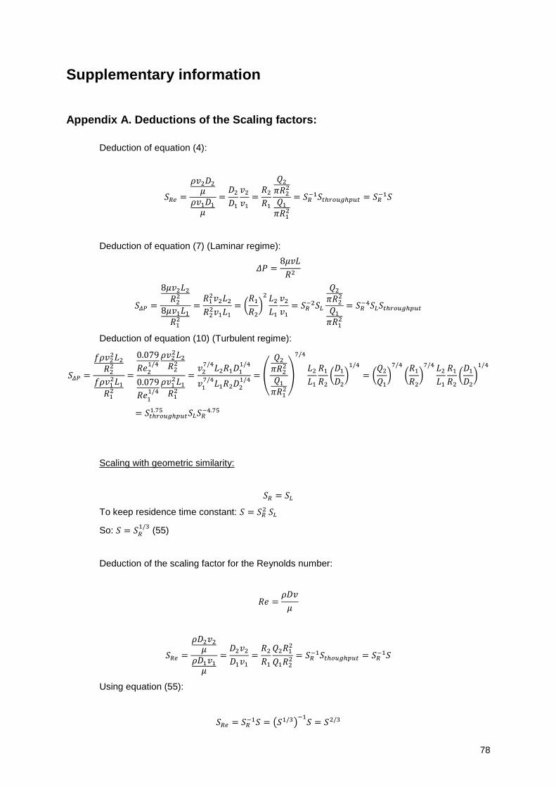
78
Supplementary information
Appendix A. Deductions of the Scaling factors:
Deduction of equation (4):
𝑆𝑅𝑒 =
𝜌𝑣2𝐷2
𝜇𝜌𝑣1𝐷1
𝜇
=𝐷2
𝐷1
𝑣2
𝑣1
=𝑅2
𝑅1
𝑄2
𝜋𝑅22
𝑄1
𝜋𝑅12
= 𝑆𝑅−1𝑆𝑡ℎ𝑟𝑜𝑢𝑔ℎ𝑝𝑢𝑡 = 𝑆𝑅
−1𝑆
Deduction of equation (7) (Laminar regime):
𝛥𝑃 =8𝜇𝑣𝐿
𝑅2
𝑆𝛥𝑃 =
8𝜇𝑣2𝐿2
𝑅22
8𝜇𝑣1𝐿1
𝑅12
=𝑅1
2𝑣2𝐿2
𝑅22𝑣1𝐿1
= (𝑅1
𝑅2
)2 𝐿2
𝐿1
𝑣2
𝑣1
= 𝑆𝑅−2𝑆𝐿
𝑄2
𝜋𝑅22
𝑄1
𝜋𝑅12
= 𝑆𝑅−4𝑆𝐿𝑆𝑡ℎ𝑟𝑜𝑢𝑔ℎ𝑝𝑢𝑡
Deduction of equation (10) (Turbulent regime):
𝑆𝛥𝑃 =
𝑓𝜌𝑣22𝐿2
𝑅22
𝑓𝜌𝑣12𝐿1
𝑅12
=
0.079
𝑅𝑒21/4
𝜌𝑣22𝐿2
𝑅22
0.079
𝑅𝑒11/4
𝜌𝑣12𝐿1
𝑅12
=𝑣2
7/4𝐿2𝑅1𝐷1
1/4
𝑣17/4
𝐿1𝑅2𝐷21/4
= (
𝑄2
𝜋𝑅22
𝑄1
𝜋𝑅12
)
7/4
𝐿2
𝐿1
𝑅1
𝑅2
(𝐷1
𝐷2
)1/4
= (𝑄2
𝑄1
)7/4
(𝑅1
𝑅2
)7/4 𝐿2
𝐿1
𝑅1
𝑅2
(𝐷1
𝐷2
)1/4
= 𝑆𝑡ℎ𝑟𝑜𝑢𝑔ℎ𝑝𝑢𝑡1.75 𝑆𝐿𝑆𝑅
−4.75
Scaling with geometric similarity:
𝑆𝑅 = 𝑆𝐿
To keep residence time constant: 𝑆 = 𝑆𝑅2 𝑆𝐿
So: 𝑆 = 𝑆𝑅1/3
(55)
Deduction of the scaling factor for the Reynolds number:
𝑅𝑒 =𝜌𝐷𝑣
𝜇
𝑆𝑅𝑒 =
𝜌𝐷2𝑣2
𝜇𝜌𝐷1𝑣1
𝜇
=𝐷2𝑣2
𝐷1𝑣1
=𝑅2
𝑅1
𝑄2𝑅12
𝑄1𝑅22 = 𝑆𝑅
−1𝑆𝑡ℎ𝑜𝑢𝑔ℎ𝑝𝑢𝑡 = 𝑆𝑅−1𝑆
Using equation (55):
𝑆𝑅𝑒 = 𝑆𝑅−1𝑆 = (𝑆1/3)
−1𝑆 = 𝑆2/3
79
Deduction of the scaling factor for the surface area:
𝐴𝑒𝑥𝑡𝑒𝑟𝑛𝑎𝑙 = 𝜋𝐷𝐿
𝑆𝐴𝑒𝑥𝑡=
𝜋𝐷2𝐿2
𝜋𝐷1𝐿1
= 𝑆𝑅𝑆𝐿
Using equation (55):
𝑆𝐴𝑒𝑥𝑡= 𝑆𝑅𝑆𝐿 = 𝑆2/3
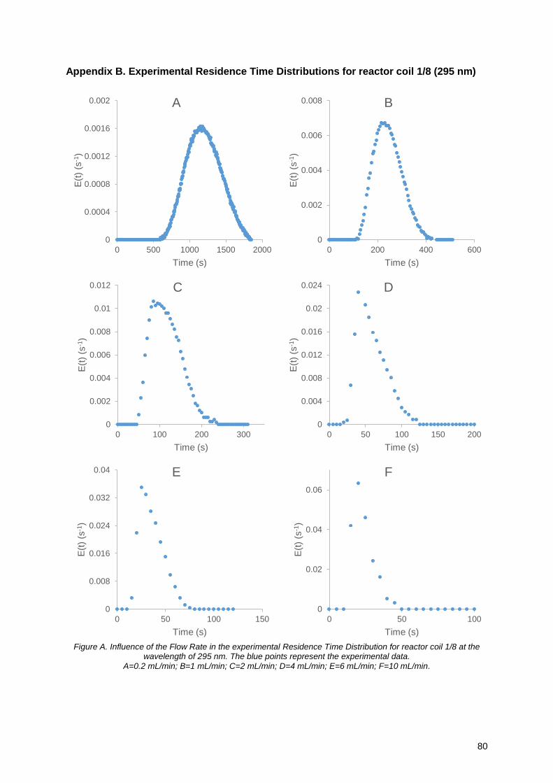
80
Appendix B. Experimental Residence Time Distributions for reactor coil 1/8 (295 nm)
Figure A. Influence of the Flow Rate in the experimental Residence Time Distribution for reactor coil 1/8 at the
wavelength of 295 nm. The blue points represent the experimental data. A=0.2 mL/min; B=1 mL/min; C=2 mL/min; D=4 mL/min; E=6 mL/min; F=10 mL/min.
0
0.0004
0.0008
0.0012
0.0016
0.002
0 500 1000 1500 2000
E(t
) (s
-1)
Time (s)
A
0
0.002
0.004
0.006
0.008
0 200 400 600
E(t
)(s
-1)
Time (s)
B
0
0.002
0.004
0.006
0.008
0.01
0.012
0 100 200 300
E(t
)(s
-1)
Time (s)
C
0
0.004
0.008
0.012
0.016
0.02
0.024
0 50 100 150 200
E(t
)(s
-1)
Time (s)
D
0
0.008
0.016
0.024
0.032
0.04
0 50 100 150
E(t
)(s
-1)
Time (s)
E
0
0.02
0.04
0.06
0 50 100
E(t
)(s
-1)
Time (s)
F
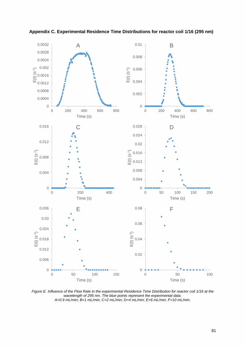
81
Appendix C. Experimental Residence Time Distributions for reactor coil 1/16 (295 nm)
Figure E. Influence of the Flow Rate in the experimental Residence Time Distribution for reactor coil 1/16 at the wavelength of 295 nm. The blue points represent the experimental data.
A=0.9 mL/min; B=1 mL/min; C=2 mL/min; D=4 mL/min; E=6 mL/min; F=10 mL/min.
0
0.0004
0.0008
0.0012
0.0016
0.002
0.0024
0.0028
0.0032
0 200 400 600 800
E(t
)(s
-1)
Time (s)
A
0
0.002
0.004
0.006
0.008
0.01
0 200 400 600 800
E(t
)(s
-1)
Time (s)
B
0
0.004
0.008
0.012
0.016
0 200 400
E(t
)(s
-1)
Time (s)
C
0
0.004
0.008
0.012
0.016
0.02
0.024
0.028
0 50 100 150 200
E(t
)(s
-1)
Time (s)
D
0
0.006
0.012
0.018
0.024
0.03
0.036
0 50 100 150
E(t
)(s
-1)
Time (s)
E
0
0.02
0.04
0.06
0.08
0 50 100
E(t
)(s
-1)
Time (s)
F
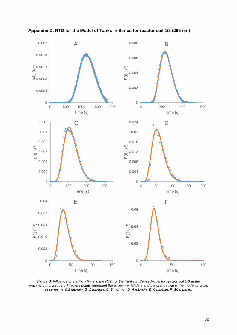
82
Appendix D. RTD for the Model of Tanks in Series for reactor coil 1/8 (295 nm)
Figure B. Influence of the Flow Rate in the RTD for the Tanks in Series Model for reactor coil 1/8 at the wavelength of 295 nm. The blue points represent the experimental data and the orange line is the model of tanks
in series. A=0.2 mL/min; B=1 mL/min; C=2 mL/min; D=4 mL/min; E=6 mL/min; F=10 mL/min.
0
0.0004
0.0008
0.0012
0.0016
0.002
0 500 1000 1500 2000
E(t
)(s
-1)
Time (s)
A
0
0.002
0.004
0.006
0.008
0 200 400 600
E(t
)(s
-1)
Time (s)
B
0
0.002
0.004
0.006
0.008
0.01
0.012
0 100 200 300
E(t
)(s
-1)
Time (s)
C
0
0.004
0.008
0.012
0.016
0.02
0.024
0 50 100 150 200
E(t
)(s
-1)
Time (s)
D
0
0.008
0.016
0.024
0.032
0.04
0 50 100 150
E(t
)(s
-1)
Time (s)
E
0
0.02
0.04
0.06
0 50 100
E(t
)(s
-1)
Time (s)
F
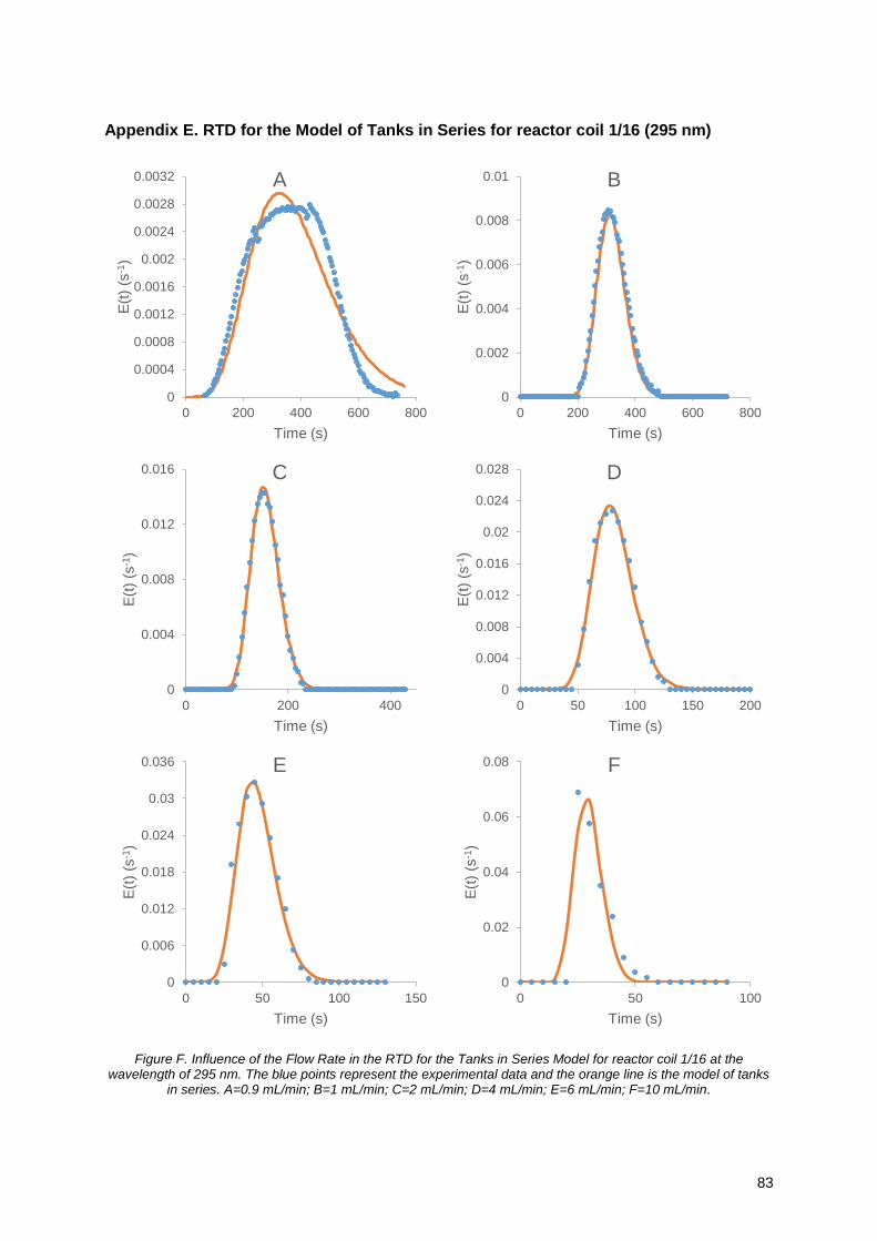
83
Appendix E. RTD for the Model of Tanks in Series for reactor coil 1/16 (295 nm)
Figure F. Influence of the Flow Rate in the RTD for the Tanks in Series Model for reactor coil 1/16 at the wavelength of 295 nm. The blue points represent the experimental data and the orange line is the model of tanks
in series. A=0.9 mL/min; B=1 mL/min; C=2 mL/min; D=4 mL/min; E=6 mL/min; F=10 mL/min.
0
0.0004
0.0008
0.0012
0.0016
0.002
0.0024
0.0028
0.0032
0 200 400 600 800
E(t
)(s
-1)
Time (s)
A
0
0.002
0.004
0.006
0.008
0.01
0 200 400 600 800
E(t
)(s
-1)
Time (s)
B
0
0.004
0.008
0.012
0.016
0 200 400
E(t
)(s
-1)
Time (s)
C
0
0.004
0.008
0.012
0.016
0.02
0.024
0.028
0 50 100 150 200
E(t
)(s
-1)
Time (s)
D
0
0.006
0.012
0.018
0.024
0.03
0.036
0 50 100 150
E(t
)(s
-1)
Time (s)
E
0
0.02
0.04
0.06
0.08
0 50 100
E(t
)(s
-1)
Time (s)
F
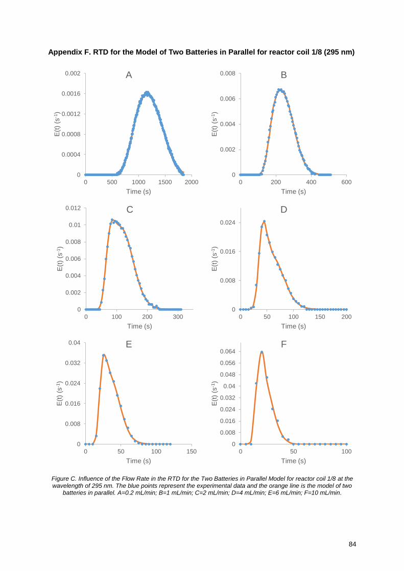
84
Appendix F. RTD for the Model of Two Batteries in Parallel for reactor coil 1/8 (295 nm)
Figure C. Influence of the Flow Rate in the RTD for the Two Batteries in Parallel Model for reactor coil 1/8 at the wavelength of 295 nm. The blue points represent the experimental data and the orange line is the model of two
batteries in parallel. A=0.2 mL/min; B=1 mL/min; C=2 mL/min; D=4 mL/min; E=6 mL/min; F=10 mL/min.
0
0.0004
0.0008
0.0012
0.0016
0.002
0 500 1000 1500 2000
E(t
)(s
-1)
Time (s)
A
0
0.002
0.004
0.006
0.008
0 200 400 600
E(t
)(s
-1)
Time (s)
B
0
0.002
0.004
0.006
0.008
0.01
0.012
0 100 200 300
E(t
)(s
-1)
Time (s)
C
0
0.008
0.016
0.024
0 50 100 150 200
E(t
)(s
-1)
Time (s)
D
0
0.008
0.016
0.024
0.032
0.04
0 50 100 150
E(t
)(s
-1)
Time (s)
E
0
0.008
0.016
0.024
0.032
0.04
0.048
0.056
0.064
0 50 100
E(t
)(s
-1)
Time (s)
F
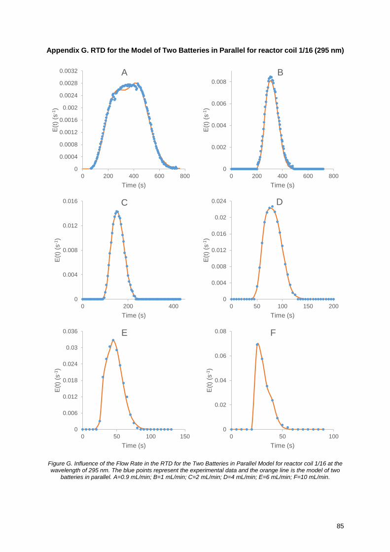
85
Appendix G. RTD for the Model of Two Batteries in Parallel for reactor coil 1/16 (295 nm)
Figure G. Influence of the Flow Rate in the RTD for the Two Batteries in Parallel Model for reactor coil 1/16 at the wavelength of 295 nm. The blue points represent the experimental data and the orange line is the model of two
batteries in parallel. A=0.9 mL/min; B=1 mL/min; C=2 mL/min; D=4 mL/min; E=6 mL/min; F=10 mL/min.
0
0.0004
0.0008
0.0012
0.0016
0.002
0.0024
0.0028
0.0032
0 200 400 600 800
E(t
)(s
-1)
Time (s)
A
0
0.002
0.004
0.006
0.008
0 200 400 600 800
E(t
)(s
-1)
Time (s)
B
0
0.004
0.008
0.012
0.016
0 200 400
E(t
)(s
-1)
Time (s)
C
0
0.004
0.008
0.012
0.016
0.02
0.024
0 50 100 150 200
E(t
)(s
-1)
Time (s)
D
0
0.006
0.012
0.018
0.024
0.03
0.036
0 50 100 150
E(t
)(s
-1)
Time (s)
E
0
0.02
0.04
0.06
0.08
0 50 100
E(t
)(s
-1)
Time (s)
F
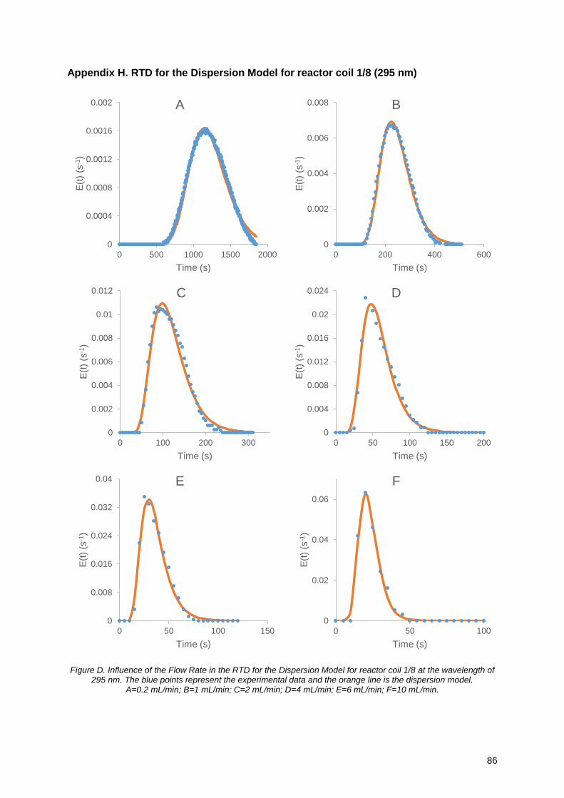
86
Appendix H. RTD for the Dispersion Model for reactor coil 1/8 (295 nm)
Figure D. Influence of the Flow Rate in the RTD for the Dispersion Model for reactor coil 1/8 at the wavelength of
295 nm. The blue points represent the experimental data and the orange line is the dispersion model. A=0.2 mL/min; B=1 mL/min; C=2 mL/min; D=4 mL/min; E=6 mL/min; F=10 mL/min.
0
0.0004
0.0008
0.0012
0.0016
0.002
0 500 1000 1500 2000
E(t
)(s
-1)
Time (s)
A
0
0.002
0.004
0.006
0.008
0 200 400 600
E(t
)(s
-1)
Time (s)
B
0
0.002
0.004
0.006
0.008
0.01
0.012
0 100 200 300
E(t
)(s
-1)
Time (s)
C
0
0.004
0.008
0.012
0.016
0.02
0.024
0 50 100 150 200
E(t
)(s
-1)
Time (s)
D
0
0.008
0.016
0.024
0.032
0.04
0 50 100 150
E(t
)(s
-1)
Time (s)
E
0
0.02
0.04
0.06
0 50 100
E(t
)(s
-1)
Time (s)
F
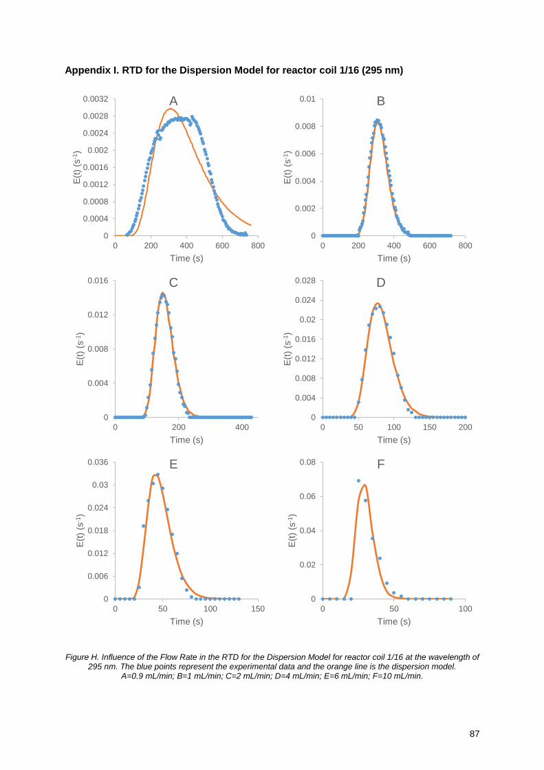
87
Appendix I. RTD for the Dispersion Model for reactor coil 1/16 (295 nm)
Figure H. Influence of the Flow Rate in the RTD for the Dispersion Model for reactor coil 1/16 at the wavelength of
295 nm. The blue points represent the experimental data and the orange line is the dispersion model. A=0.9 mL/min; B=1 mL/min; C=2 mL/min; D=4 mL/min; E=6 mL/min; F=10 mL/min.
0
0.0004
0.0008
0.0012
0.0016
0.002
0.0024
0.0028
0.0032
0 200 400 600 800
E(t
)(s
-1)
Time (s)
A
0
0.002
0.004
0.006
0.008
0.01
0 200 400 600 800
E(t
)(s
-1)
Time (s)
B
0
0.004
0.008
0.012
0.016
0 200 400
E(t
)(s
-1)
Time (s)
C
0
0.004
0.008
0.012
0.016
0.02
0.024
0.028
0 50 100 150 200
E(t
)(s
-1)
Time (s)
D
0
0.006
0.012
0.018
0.024
0.03
0.036
0 50 100 150
E(t
)(s
-1)
Time (s)
E
0
0.02
0.04
0.06
0.08
0 50 100
E(t
)(s
-1)
Time (s)
F
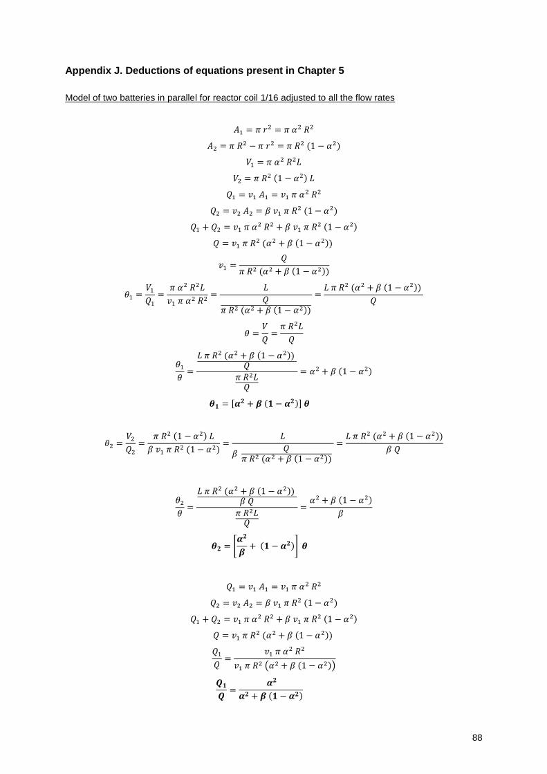
88
Appendix J. Deductions of equations present in Chapter 5
Model of two batteries in parallel for reactor coil 1/16 adjusted to all the flow rates
𝐴1 = 𝜋 𝑟2 = 𝜋 𝛼2 𝑅2
𝐴2 = 𝜋 𝑅2 − 𝜋 𝑟2 = 𝜋 𝑅2 (1 − 𝛼2)
𝑉1 = 𝜋 𝛼2 𝑅2𝐿
𝑉2 = 𝜋 𝑅2 (1 − 𝛼2) 𝐿
𝑄1 = 𝑣1 𝐴1 = 𝑣1 𝜋 𝛼2 𝑅2
𝑄2 = 𝑣2 𝐴2 = 𝛽 𝑣1 𝜋 𝑅2 (1 − 𝛼2)
𝑄1 + 𝑄2 = 𝑣1 𝜋 𝛼2 𝑅2 + 𝛽 𝑣1 𝜋 𝑅2 (1 − 𝛼2)
𝑄 = 𝑣1 𝜋 𝑅2 (𝛼2 + 𝛽 (1 − 𝛼2))
𝑣1 =𝑄
𝜋 𝑅2 (𝛼2 + 𝛽 (1 − 𝛼2))
𝜃1 =𝑉1
𝑄1
=𝜋 𝛼2 𝑅2𝐿
𝑣1 𝜋 𝛼2 𝑅2=
𝐿
𝑄𝜋 𝑅2 (𝛼2 + 𝛽 (1 − 𝛼2))
=𝐿 𝜋 𝑅2 (𝛼2 + 𝛽 (1 − 𝛼2))
𝑄
𝜃 =𝑉
𝑄=
𝜋 𝑅2𝐿
𝑄
𝜃1
𝜃=
𝐿 𝜋 𝑅2 (𝛼2 + 𝛽 (1 − 𝛼2)) 𝑄
𝜋 𝑅2𝐿𝑄
= 𝛼2 + 𝛽 (1 − 𝛼2)
𝜽𝟏 = [𝜶𝟐 + 𝜷 (𝟏 − 𝜶𝟐)] 𝜽
𝜃2 =𝑉2
𝑄2
=𝜋 𝑅2 (1 − 𝛼2) 𝐿
𝛽 𝑣1 𝜋 𝑅2 (1 − 𝛼2)=
𝐿
𝛽 𝑄
𝜋 𝑅2 (𝛼2 + 𝛽 (1 − 𝛼2))
=𝐿 𝜋 𝑅2 (𝛼2 + 𝛽 (1 − 𝛼2))
𝛽 𝑄
𝜃2
𝜃=
𝐿 𝜋 𝑅2 (𝛼2 + 𝛽 (1 − 𝛼2)) 𝛽 𝑄
𝜋 𝑅2𝐿𝑄
=𝛼2 + 𝛽 (1 − 𝛼2)
𝛽
𝜽𝟐 = [𝜶𝟐
𝜷+ (𝟏 − 𝜶𝟐)] 𝜽
𝑄1 = 𝑣1 𝐴1 = 𝑣1 𝜋 𝛼2 𝑅2
𝑄2 = 𝑣2 𝐴2 = 𝛽 𝑣1 𝜋 𝑅2 (1 − 𝛼2)
𝑄1 + 𝑄2 = 𝑣1 𝜋 𝛼2 𝑅2 + 𝛽 𝑣1 𝜋 𝑅2 (1 − 𝛼2)
𝑄 = 𝑣1 𝜋 𝑅2 (𝛼2 + 𝛽 (1 − 𝛼2))
𝑄1
𝑄=
𝑣1 𝜋 𝛼2 𝑅2
𝑣1 𝜋 𝑅2 (𝛼2 + 𝛽 (1 − 𝛼2))
𝑸𝟏
𝑸=
𝜶𝟐
𝜶𝟐 + 𝜷 (𝟏 − 𝜶𝟐)
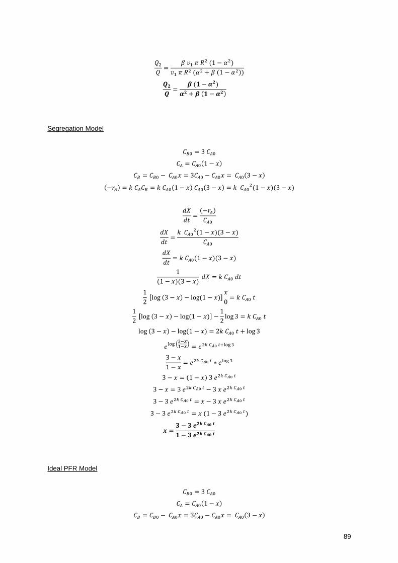
89
𝑄2
𝑄=
𝛽 𝑣1 𝜋 𝑅2 (1 − 𝛼2)
𝑣1 𝜋 𝑅2 (𝛼2 + 𝛽 (1 − 𝛼2))
𝑸𝟐
𝑸=
𝜷 (𝟏 − 𝜶𝟐)
𝜶𝟐 + 𝜷 (𝟏 − 𝜶𝟐)
Segregation Model
𝐶𝐵0 = 3 𝐶𝐴0
𝐶𝐴 = 𝐶𝐴0(1 − 𝑥)
𝐶𝐵 = 𝐶𝐵0 − 𝐶𝐴0𝑥 = 3𝐶𝐴0 − 𝐶𝐴0𝑥 = 𝐶𝐴0(3 − 𝑥)
(−𝑟𝐴) = 𝑘 𝐶𝐴𝐶𝐵 = 𝑘 𝐶𝐴0(1 − 𝑥) 𝐶𝐴0(3 − 𝑥) = 𝑘 𝐶𝐴02(1 − 𝑥)(3 − 𝑥)
𝑑𝑋
𝑑𝑡=
(−𝑟𝐴)
𝐶𝐴0
𝑑𝑋
𝑑𝑡=
𝑘 𝐶𝐴02(1 − 𝑥)(3 − 𝑥)
𝐶𝐴0
𝑑𝑋
𝑑𝑡= 𝑘 𝐶𝐴0(1 − 𝑥)(3 − 𝑥)
1
(1 − 𝑥)(3 − 𝑥) 𝑑𝑋 = 𝑘 𝐶𝐴0 𝑑𝑡
1
2 [log (3 − 𝑥) − log (1 − 𝑥)]
𝑥
0= 𝑘 𝐶𝐴0 𝑡
1
2 [log (3 − 𝑥) − log (1 − 𝑥)] −
1
2log 3 = 𝑘 𝐶𝐴0 𝑡
log (3 − 𝑥) − log (1 − 𝑥) = 2𝑘 𝐶𝐴0 𝑡 + log 3
𝑒log (3−𝑥1−𝑥
) = 𝑒2𝑘 𝐶𝐴0 𝑡+log 3
3 − 𝑥
1 − 𝑥= 𝑒2𝑘 𝐶𝐴0 𝑡 ∗ 𝑒log 3
3 − 𝑥 = (1 − 𝑥) 3 𝑒2𝑘 𝐶𝐴0 𝑡
3 − 𝑥 = 3 𝑒2𝑘 𝐶𝐴0 𝑡 − 3 𝑥 𝑒2𝑘 𝐶𝐴0 𝑡
3 − 3 𝑒2𝑘 𝐶𝐴0 𝑡 = 𝑥 − 3 𝑥 𝑒2𝑘 𝐶𝐴0 𝑡
3 − 3 𝑒2𝑘 𝐶𝐴0 𝑡 = 𝑥 (1 − 3 𝑒2𝑘 𝐶𝐴0 𝑡)
𝒙 =𝟑 − 𝟑 𝒆𝟐𝒌 𝑪𝑨𝟎 𝒕
𝟏 − 𝟑 𝒆𝟐𝒌 𝑪𝑨𝟎 𝒕
Ideal PFR Model
𝐶𝐵0 = 3 𝐶𝐴0
𝐶𝐴 = 𝐶𝐴0(1 − 𝑥)
𝐶𝐵 = 𝐶𝐵0 − 𝐶𝐴0𝑥 = 3𝐶𝐴0 − 𝐶𝐴0𝑥 = 𝐶𝐴0(3 − 𝑥)
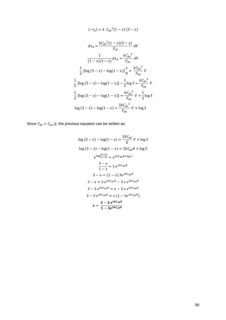
90
(−𝑟𝐴) = 𝑘 𝐶𝐴02(1 − 𝑥) (3 − 𝑥)
𝑑𝑥𝐴 =𝑘𝐶𝐴0
2(1 − 𝑥)(3 − 𝑥)
𝐹𝐴0
𝑑𝑉
1
(1 − 𝑥)(3 − 𝑥)𝑑𝑥𝐴 =
𝑘𝐶𝐴02
𝐹𝐴0
𝑑𝑉
1
2 [log (3 − 𝑥) − log (1 − 𝑥)]
𝑥
0=
𝑘𝐶𝐴02
𝐹𝐴0
𝑉
1
2 [log (3 − 𝑥) − log (1 − 𝑥)] −
1
2log 3 =
𝑘𝐶𝐴02
𝐹𝐴0
𝑉
1
2 [log (3 − 𝑥) − log (1 − 𝑥)] =
𝑘𝐶𝐴02
𝐹𝐴0
𝑉 +1
2log 3
log (3 − 𝑥) − log (1 − 𝑥) =
2𝑘𝐶𝐴02
𝐹𝐴0
𝑉 + log 3
Since 𝐹𝐴0 = 𝐶𝐴0 𝑄, the previous equation can be written as:
log (3 − 𝑥) − log (1 − 𝑥) =2𝑘𝐶𝐴0
𝑄 𝑉 + log 3
log (3 − 𝑥) − log (1 − 𝑥) = 2𝑘𝐶𝐴0𝜃 + log 3
𝑒log(3−𝑥1−𝑥
) = 𝑒2𝑘𝐶𝐴0𝜃+log 3
3 − 𝑥
1 − 𝑥= 3 𝑒2𝑘𝐶𝐴0𝜃
3 − 𝑥 = (1 − 𝑥) 3𝑒2𝑘𝐶𝐴0𝜃
3 − 𝑥 = 3 𝑒2𝑘𝐶𝐴0𝜃 − 3 𝑥 𝑒2𝑘𝐶𝐴0𝜃
3 − 3 𝑒2𝑘𝐶𝐴0𝜃 = 𝑥 − 3 𝑥 𝑒2𝑘𝐶𝐴0𝜃
3 − 3 𝑒2𝑘𝐶𝐴0𝜃 = 𝑥 (1 − 3𝑒2𝑘𝐶𝐴0𝜃)
𝒙 = 𝟑 − 𝟑 𝒆𝟐𝒌𝑪𝑨𝟎𝜽
𝟏 − 𝟑𝒆𝟐𝒌𝑪𝑨𝟎𝜽