Seediscussions,stats,andauthorprofilesforthispublicationat:http://www.researchgate.net/publication/236902025

Characterizationoftillageeffectsonthespatialvariationofsoilpropertiesusingground-penetratingradarandelectromagneticinduction

ARTICLEinGEODERMA·JANUARY2012

ImpactFactor:2.51

CITATIONS

5

DOWNLOADS

14

VIEWS

54

8AUTHORS,INCLUDING:

M.R.M.Ardekani

InneauTech

26PUBLICATIONS63CITATIONS

SEEPROFILE

C.Roisin

WalloonAgriculturalResearchCentreCRA-W

18PUBLICATIONS31CITATIONS

SEEPROFILE

JulienMinet

UniversityofLiège

24PUBLICATIONS141CITATIONS

SEEPROFILE

S.Lambot

CatholicUniversityofLouvain

115PUBLICATIONS1,201CITATIONS

SEEPROFILE

Availablefrom:M.R.M.Ardekani

Retrievedon:15July2015

Geoderma 207–208 (2013) 310–322

Contents lists available at SciVerse ScienceDirect

Geoderma

j ourna l homepage: www.e lsev ie r .com/ locate /geoderma

Characterization of tillage effects on the spatial variation of soilproperties using ground-penetrating radar andelectromagnetic induction

François Jonard a,⁎, Mohammad Mahmoudzadeh b, Christian Roisin c, Lutz Weihermüller a,Frédéric André b, Julien Minet b, Harry Vereecken a, Sébastien Lambot b

a Agrosphere (IBG-3), Institute of Bio- and Geosciences, Forschungszentrum Jülich GmbH, 52425 Jülich, Germanyb Earth and Life Institute, Université catholique de Louvain, Croix du Sud 2 Box L7.05.02, 1348 Louvain-la-Neuve, Belgiumc Agriculture and Natural Environment Department, Walloon Agricultural Research Centre, rue du Bordia 4, 5030 Gembloux, Belgium

⁎ Corresponding author. Tel.: +49 2461 61 9518; faxE-mail address: f.jonard@fz-juelich.de (F. Jonard).

0016-7061/$ – see front matter © 2013 Elsevier B.V. Allhttp://dx.doi.org/10.1016/j.geoderma.2013.05.024

a b s t r a c t

a r t i c l e i n f o

Article history:Received 16 March 2012Received in revised form 14 May 2013Accepted 27 May 2013Available online xxxx

Keywords:Soil tillageGround-penetrating radarElectromagnetic inductionDigital soil mappingSoil water contentSoil resistance

Tillage practices influence physical, chemical, and biological soil properties, which also affect soil quality andconsequently plant growth. In this study, the main objective was to evaluate the effects of different tillagepractices on soil physical properties such as soil water content (SWC) by using geophysical methods, namely,ground-penetrating radar (GPR) and electromagnetic induction (EMI). Additional measurements such as soilsampling, capacitance probe, and soil penetrometer data were acquired as ground truths. The study wasperformed for three contrasting tillage practices, i.e., conventional tillage (CT), deep loosening tillage (DL),and reduced tillage (RT), applied on different plots of an agricultural field. The data showed that tillageinfluences soil resistance in shallow soil layers (deeper tillage decreases soil resistance), which could be partlyseen in on-ground GPR data. In addition, reference SWC measurements (capacitance probes and soil sampling)were in fairly good agreement with the water content estimates from off-ground GPR. We also observed atillage effect on shallow surface SWC, while deeper SWC seems to be unaffected by tillage. Mean surface SWCwas significantly lower for CT compared to DL and RT, which was partly explained by lower pore connectivitybetween the topsoil and the deeper layers after conventional tillage. Moreover, the variance of the SWC withinthe conventional tillage plots was larger than within the other plots. This larger SWC variability could beexplained by a greater soil heterogeneity induced by the plowing process. Overall, this study confirms the po-tential of GPR and EMI for the determination of soil physical properties at the field scale and for the assessmentof agricultural management practices.

© 2013 Elsevier B.V. All rights reserved.

1. Introduction

Agricultural management practices can affect soil physical, chem-ical, and biological properties with consequences for the movementof water, nutrients, and pollutants in the vadose zone, and for plantgrowth (Strudley et al., 2008). Alternative management practicessuch as conservation tillage or reduced tillage are encouraged toprevent environmental risks like soil erosion, flooding, and pesticideleaching in the groundwater. However, producers are reluctant toadopt these practices as their effects on soil and crop production arenot yet well understood (Alletto et al., 2011). The impact of tillagepractices on soil hydraulic properties (Ndiaye et al., 2007; Sauer etal., 1990; Schwen et al., 2011a,b; Strudley et al., 2008) and their

: +49 2461 61 2518.

rights reserved.

consequences on preferential flow (Elliott et al., 2000; Kulasekera etal., 2011), soil state variables (soil water content and soil tempera-ture) (Kovar et al., 1992; Tan et al., 2002), soil physical properties(soil penetration resistance, soil bulk density, soil porosity) (Jabro etal., 2009), and plant growth (Alletto et al., 2011; Zhang et al., 2011)have been subject to intensive research over the past decade. How-ever, according to the recent review by Strudley et al. (2008),experimental results from field and laboratory studies do not showconsistent effects of tillage practices on soil properties. Moreover, toobtain information about soil properties, most of these studies usedinvasive methods such as time-domain reflectometry, capacitancesensors, or soil sampling, which are time-consuming and offer onlylocal information. Therefore, these techniques are limited to a smallspatial extent. In addition, time-lapse measurements are not feasiblewithin agricultural fields, although they would provide valuable in-sights into the changes of the state variables (e.g., soil water contentand soil temperature) or the processes involved.

311F. Jonard et al. / Geoderma 207–208 (2013) 310–322

In that respect, ground-penetrating radar (GPR) and electromag-netic induction (EMI) are non-invasive geophysical techniques whichcan be used to characterize the shallow subsurface properties at thefield scale with high temporal and spatial resolutions (André et al.,2012; Cockx et al., 2007; Huisman et al., 2003; Jonard et al., 2011;Lambot et al., 2008; Slob et al., 2010). EMI is sensitive to soil electricalconductivity, which is mainly affected by soil water content (SWC),clay content, and salinity (Corwin and Lesch, 2005; Friedman, 2005),while GPR is sensitive to both soil electrical conductivity and dielectricpermittivity, the latter primarily depending on SWC (Topp et al., 1980).Yet, until now, very few studies have used geophysical techniques toinvestigate the impact of tillage practices (e.g., Basso et al., 2011;Oleschko et al., 2008; Richard et al., 2010). Recently, Müller et al.(2009) compared different geophysical techniques to characterizetillage effects on SWC and electrical resistivity. However, their sam-pling scheme was limited to two transects, which did not permitthem to fully explain their observations. Basso et al. (2011) usedelectrical resistivity tomography applied to an entire field area, whichenabled them to study the spatiotemporal dynamics of soil physicalproperties. Nevertheless, a high resolution could not be achieved, espe-cially at the soil surface.

The general objective of this present study is to analyze the effectsof tillage practices on the spatial variation of soil properties by usinggeophysical techniques. In particular, we focused on surface SWC,bulk soil electrical conductivity, and mechanical resistance. The studywas conducted on an agricultural field in the loess belt of central Bel-gium (Gentinnes). GPR and EMI measurements were performed forthree contrasting tillage practices, i.e., conventional tillage (CT), deeploosening tillage (DL), and reduced tillage (RT). In this paper, we firstpresent on-ground GPR images and soil strength maps to characterizethe tillage effect on soil penetration resistance. Soil electrical conduc-tivity and SWC maps from EMI and off-ground GPR data, respectively,are then presented and interpreted in the light of in situ observations.Finally, the tillage effect on SWC and its spatial distribution isdiscussed.

2. Materials and methods

2.1. Experimental site

The study was conducted on an agricultural field in Gentinnes,located in the loess belt of central Belgium (50°35′ N 4°35′ E). Thesoil is a silty loam soil classified as an Orthic Luvisol according to theFAO classification. Elevation varies between 137 and 145 m above sealevel. The silt fraction dominates the clay and sand fractions (20.0,74.5, and 5.5% for clay, silt, and sand, respectively) in the topsoil(0–25 cm), and the organic carbon content was 8.67 g kg−1. Theexact water table depth is unknown, but is in general deeper than2 m. Since fall 2005, a soil tillage experiment has been implementedon the field to compare three contrasting tillage systems: (1) conven-tional tillage (CT) with moldboard plowing to ≈27 cm depth, (2)deep loosening tillage (DL) with a heavy tine cultivator to ≈30 cmdepth, and (3) reduced tillage (RT) with a spring tine cultivator to≈10 cm depth. The field was divided into 20 plots of 30 × 18 m2

and each plot was characterized by one of the three tillage systems(Fig. 1). Only 12 plots were used for the geophysical measurements(4 replications per tillage system) and 3 other plots were used for thesoil strength measurements. These 3 plots were located next to the12 other plots, at a distance of about 15 m in the south-western partof the field (not shown in Fig. 1). The geophysical measurementswere performed on April 13, 2010, while the soil strength measure-ments were performed on April 27, 2010. Average monthly rainfallrecorded at a meteorological station located about 7 km away fromthe field was 75.3 mm in February, 36.0 mm in March, and 23.4 mmin April 2010. No rain was observed during the two measurement

days and the daily reference evapotranspiration was close to 3 mmfor both dates (Fig. 2).

2.2. Agricultural practices

Initially, the study site had been plowed in its entirety for severaldecades. Since 2005, it has been divided according to three tillage sys-tems (CT, DL, and RT) and the same tillage treatment has been appliedevery year to the same plot, except in 2006 and 2008, where the DLtillage system was replaced by the RT tillage system. In 2006 and2008, sugar beet was planted in April after seed bed preparation(with rotary harrow and drill), while winter wheat was sown inNovember (also with rotary harrow and drill). The wheat straw waschopped during the harvest and then mixed into the top soil layerby stubble harrowing. White mustard was used as a cover crop forall the plots during three fallow periods (2005–2006, 2007–2008,2009–2010), i.e., before sugar beet planting. Whitemustard was alwayssown in September using rotary harrow and drill. The three tillagetreatments (CT, DL, and RT) were systematically applied before sowingwhite mustard or winter wheat. In April 2010, one day before the geo-physical measurements, a minimum tillage was applied to all the plotswith a disk harrow (to a depth of 5 cm) in order to reduce soil surfaceroughness for the radar measurements (Jonard et al., 2012). The dayafter the geophysical measurements, the whole field was preparedfor seed bed with a disk harrow (to a depth of 3 cm) and flax wassown.

2.3. Reference soil water content measurements

Undisturbed soil samples (100 cm3 Kopecky rings) were used asreference measurements for the volumetric SWC. Soil samples werecollected between 0 and 5 cm depth on a regular grid in each plot(5 × 3 m spacing, i.e., 35 samples per plot and 420 samples intotal). Soil samples were also taken at two locations in each plotbetween 0 and 75 cm depth in 5 cm steps. The two locations werechosen arbitrarily around the middle of each plot. The volumetricwater content of the soil samples was obtained by the weight lossafter oven drying at 105 °C for at least 48 h. At each sampling point,soil dielectric permittivity was measured using two capacitancesensors, namely, the ThetaProbe ML2x sensor (Delta-T Devices Ltd,Cambridge, UK) and the 5TE sensor (Decagon Devices Inc.,Pullman, Washington, USA), which were inserted vertically into thesoil. The ThetaProbe sensor operates at 100 MHz and has four stain-less steel rods of 6 cm length while the 5TE probe operates at afrequency of 70 MHz and has 3 prongs of 5.2 cm length. Threemeasurements with each probe were performed at a distance of lessthan 15 cm around each sampling point. The soil water content wasthen determined from the soil dielectric permittivity using Topp'smodel (Topp et al., 1980). It should be noted that using a site-specific relationship or a dielectric mixing model instead of Topp'smodel is likely to provide better absolute results. Nevertheless, Topp'smodel was chosen due to its simple application and because thepresent study is mainly focused on the comparison of SWC valueswith respect to different tillage treatments, which means that relativedifferences can be used.

2.4. Geophysical measurements

2.4.1. Ground-penetrating radarsTwo different ground-penetrating radar (GPR) systems were used

in this study: (1) off-ground radar for SWC retrieval and (2) commonon-ground radar for soil stratigraphy imaging, whereby both radarsystems were set up on an all-terrain vehicle (ATV) (Fig. 3).

2.4.1.1. Off-ground GPR. The radar system was set up using a ZVLvector network analyzer (VNA, Rohde & Schwarz, Munich, Germany),

166000

166000

166040

166040

166080

166080

166120

166120

1419

10

1419

10

1419

40

1419

40

1419

70

1419

70

1420

00

1420

00

1420

30

1420

30

0 25 5012.5Meters

Tillage systemsConventional Tillage

Deep Loosening Tillage

Reduced Tillage

Ground-truth data

Off-ground GPR data

On-ground GPR transects

Projected Coordinate System: Belgian Lambert 1972Projection: Lambert Conformal ConicEllipsoid : Hayford 1924Datum: Belgian Datum 1972

Experimental Setup

Fig. 1. Study site at Gentinnes, Belgium. Sampling points for the reference measurements and the off-ground GPR data acquisition are shown. The location of the three selectedon-ground GPR transects (see Fig. 6) is also shown. Background colors represent the three tillage systems: conventional tillage, deep loosening tillage, and reduced tillage.

312 F. Jonard et al. / Geoderma 207–208 (2013) 310–322

thereby providing an ultrawideband (UWB) stepped-frequencycontinuous-wave (SFCW) radar. The antenna system consisted of atransverse electromagnetic (TEM), double-ridged broadband hornantenna (BBHA 9120 F, Schwarzbeck Mess-Elektronik, Schönau,Germany). The antennawas 95 cm longwith a 68 × 96 cm2 aperturearea and a −3 dB full beamwidth in the E-plane and the H-planeof 46° (at 400 MHz). The antenna nominal frequency range was0.2–2 GHz and its isotropic gain ranged from 9 to 14 dBi.

With this radar system, the raw data consist of the frequency-dependent complex ratio S11 between the backscattered electromag-netic field (b(ω)) and the incident electromagnetic field (a(ω)), withω being the angular frequency. The raw GPR data were obtainedsequentially at 301 stepped operating frequencies over the range

0.2–2 GHz with a frequency step of 6 MHz. Only lower frequencydata (0.2–0.4 GHz), which were not affected by soil surface rough-ness, were used for the inversions. Assuming that the distribution ofthe electromagnetic field measured by the antenna is independentof the scatterer, i.e., only the phase and amplitude of the field change(plane wave approximation over the antenna aperture), the followingradar equation applies (Lambot et al., 2004):

S11 ωð Þ ¼ b ωð Þa ωð Þ ¼ Hi ωð Þ þ H ωð ÞG↑

xx ωð Þ1−Hf ωð ÞG↑

xx ωð Þ ð1Þ

whereHi(ω) is the antenna return loss,H(ω) is the antenna transmitting–receiving transfer function, Hf(ω) is the antenna feedback loss, and

1 5 10 15 20 25 300

2

4

6

8

10

Days in April 2010

P [m

m]

↓A

↓B

ET

o [m

m]

0

2

4

6

8

10

Fig. 2. Daily rainfall (P) and daily reference evapotranspiration (ETo) in mm measuredat the Ernage–Gembloux weather station during April 2010. Arrows indicate the first(A) and second (B) measurement day.

313F. Jonard et al. / Geoderma 207–208 (2013) 310–322

Gxx↑ (ω) is the transfer Green's function of the air–soil system. The

Green's function represents a solution of the 3D Maxwell equationsfor electromagnetic waves propagating in multilayered media(Michalski and Mosig, 1997).

In order to identify the surface dielectric permittivity, inversion ofthe Green's function is performed in the time domain, focusing on atime window containing the surface reflection only (Lambot et al.,2006). The inverse problem is formulated in the least-squares senseand the objective function to be minimized is defined accordingly asfollows:

ϕ bð Þ ¼ g↑�xx−g↑xx� �T ⋅ g↑�xx−g↑xx

� �ð2Þ

where

g↑�xx ¼ g↑�xx tð Þjtmaxtmin

and g↑xx ¼ g↑xx tð Þjtmaxtmin

ð3Þ

are the vectors containing, respectively, the observed and simulatedtime-domain windowed Green's functions, and b = [εr,ha] is the

On-ground GPR antennas

GPS antennas

Off-ground GPR antenna

EM38

Profiler

Vector network analyzer

Fig. 3. Off-ground GPR (horn antenna linked to a vector network analyzer, DGPS de-vice, and a PC), on-ground GPR, and the EM38 sensor mounted on an all-terrain vehicleas well as the Profiler sensor carried manually.

parameter vector to be estimated, with εr [dimensionless] being thesoil surface relative dielectric permittivity and ha [m] being thedistance between the antenna phase center and the soil surface. Asfor the capacitance water content sensors, the water content wasderived from the dielectric permittivity using Topp's model.

2.4.1.2. On-ground GPR. We used a time-domain GPR system (modelSIR-20, Geophysical Survey Systems, Inc., Salem, Massachusetts,USA) combined with a transmitting (Tx) and receiving (Rx)400 MHz center-frequency-shielded bowtie antenna with a Tx andRx offset of 0.16 m. GPR data were collected with a sampling intervalof 5 cm, and 512 samples per scan were recorded with 16 bits persample. The GPR produces a Ricker-type pulse with a frequency band-width of 100–800 MHz. The gain function was enabled at 5 points inorder to highlight deeper reflections. The time windowwas limited to50 ns. The on-ground GPR was used for soil imaging only (data werenot inverted). It is worth noting that we did not use the data from thebistatic radar configuration (1.10 m Tx–Rx offset) shown in Fig. 3.

2.4.2. Electromagnetic inductionEMI data were acquired with the Profiler EMP-400 (Geophysical

Survey Systems, Inc., Salem, Massachusetts, USA) and the EM38(Geonics Limited, Mississauga, Ontario, Canada) sensors. The Profilerwas manually carried at about 0.10 m above the ground surface andallowed to perform measurements simultaneously at three differentfrequencies: 5, 10, and 15 kHz. The data were recorded every second,corresponding to an average sampling interval of about 0.80 m. Incontrast, the EM38 was mounted on the front of the ATV at about0.30 m above the ground surface (see Fig. 3) and the data wererecorded at one frequency only (14.7 kHz). The EM38 was fixed at asufficient distance (about 1.30 m) from the ATV to avoid interfer-ences. Profiler data were collected with both horizontal and verticaldipole orientations, while EM38 measurements were performedwith vertical dipole orientation only. The use of different frequenciesand dipole orientations permitted different soil depths to be investi-gated. All equipment (GPR and EMI sensors) was georeferenced bymeans of a differential global positioning system (DGPS).

2.5. Soil strength measurements

The soil strength measurements were performed in three plotscharacterized by the three tillage methods and located next to thetwelve plots previously investigated. These measurements wereperformed two weeks after the geophysical measurements. A fullyautomated penetrometer (30° angle cone with a base area of 1 cm2)mounted on a small vehicle was used as described by Roisin (2007)(Fig. 4). Two areas of 80 × 80 cm2 located side by side were investi-gated. These two squares were divided along a 16 × 16 lattice (with5 cm spacing between neighboring points) yielding a total of 256nodes each. At each node, a penetration was performed, and datawere collected every centimeter from the surface down to a depthof 45 cm. This procedure resulted in a 32 × 32 matrix of resistancevalues at each of 45 depth levels.

2.6. Statistical analysis

A linear mixed model was used to test for the effects of tillage treat-ment and sensor on the soil volumetric water content (θ [m3 m−3]):

θijk ¼ μ þ αi þ βj þ γij þ εijk ð4Þ

where μ is the total mean θ, αi is the sensor effect with i levels (i = 1for ThetaProbe, 2 for 5TE, 3 for soil sampling, and 4 for off-groundGPR), βj is the tillage effect with j levels (j = 1 for CT, 2 for DL, and 3for RT), γij is the interaction term between sensor and tillage, and εijk

Fig. 4. Fully automated penetrometer used for the soil strength measurements.

0 20 40 60 80 100 120 140 160

−40

−30

−20

−10

0

Distance [cm]

Dep

th [

cm]

0

2

4

[MPa]

0 20 40 60 80 100 120 140 160

−40

−30

−20

−10

0

Distance [cm]

Dep

th [

cm]

0

2

4

[MPa]

0 20 40 60 80 100 120 140 160

−40

−30

−20

−10

0

Distance [cm]

Dep

th [

cm]

0

2

4

[MPa]

a

b

c

Fig. 5. 2D soil strength maps obtained by the penetrometer after (a) conventional till-age, (b) deep loosening tillage, and (c) reduced tillage.

314 F. Jonard et al. / Geoderma 207–208 (2013) 310–322

is the residual term for the kth observation of the ith and jth sensor andtillage levels, respectively.

A linear mixed model was also used to test for the effects of tillagetreatment, sensor, and sensor operating frequency on the soil apparentelectrical conductivity (σ [mS m−1]):

σ ijke ¼ μ þ αi þ βj þ γk þ δij þ ζ ik þ ηjk þ νijk þ εijke ð5Þ

where μ is the total mean σ, αi is the sensor effect with i levels (i = 1for EM38, 2 for Profiler with horizontal dipoles, and 3 for Profiler withvertical dipoles), βj is the frequency effect with j levels (j = 1 for5 kHz, 2 for 10 kHz, 3 for 15 kHz, and 4 for 14.7 kHz), γk is the tillageeffect with k levels (k = 1 for CT, 2 for DL, and 3 for RT), δij is the inter-action term between sensor and frequency, ζik is the interaction termbetween sensor and tillage, ηjk is the interaction term between fre-quency and tillage, vijk is the triple interaction term, and εijke is the re-sidual term for the eth observation of the ith sensor level, the jthfrequency level, and the kth tillage level.

In these models, α, β, γ, δ, ζ, η, and v were considered as linearfixed effects and the spatial correlation among the data was takeninto account by considering a covariance pattern with an exponentialstructure for the residuals (Brown and Prescott, 2006). The modelswere fitted using the MIXED procedure of the SAS software (Version9.3; SAS Institute Inc., Cary, North Carolina, USA). The fitted modelswere selected on the basis of the Akaike information criterion (AIC).Weak collinearity between independent variables was checked, aswere residual homoscedasticity and residual normal distribution.Contrasts were used to test the differences between tillage treat-ments for a given sensor (Eq. (4)) or for a given sensor and frequency(Eq. (5)). All statistical tests were performed at a 0.05 significancelevel.

3. Results and discussion

3.1. Shallow soil stratigraphy imaging

First, we analyzed the shallow soil stratigraphy using the 2D soilstrength maps as depicted in Fig. 5 obtained by the penetrometer forthe three different tillage systems (CT, DL, and RT). It should be notedthat the 2D vertical profiles were calculated by averaging the datacollected in 3D over one direction (y-axis) for better visualization. Inall cases, the profiles are depicted in the perpendicular direction ofthe tillage practice to highlight the tillage effect on soil resistance.Fig. 5a clearly shows two distinct layers for the CT, whereby the firstlayer (0–25 cm depth) is characterized by lower resistance values

(b2.5 MPa) compared to the second layer with resistance values ex-ceeding 2.5 MPa. The lower resistance value of the first layer can beexplained by the plowing, which generally reduces soil compaction inthe top layer. In general, the resistance of the first layer is quite homo-geneous, but on the top left (between the distances of 20 and 80 cm)two blocks with higher resistance can be observed which correspondto areas of compaction below the tractor tracks. The second layerwith generally higher compaction values indicates a clear stratigraphicincrease of resistance with depth. The DL map (Fig. 5b) also shows twodistinct layers, but with less clear separation and greater heterogeneity.The uneven separation of the layering can also be explained by the till-age practice, whereby the two main prongs of the heavy tine cultivatorcaused the local changes during the deep loosening. Nevertheless, alayer separation can be detected between 20 and 25 cm depth. Incomparison to CT and DL, RT (Fig. 5c) shows a much finer top layer(about 10 cm depth), which can be related to the smaller penetrationdepth of the tine cultivator used for the reduced tillage. Additionally,the top layer is highly homogeneous. The irregularities observed inthe second layer at about 20 cmdepth can be attributed to previous till-age practices before 2005. These irregularities are not visible in the CTand DL plots because the plowing and deep loosening are both below20 cmdepth. In general, the penetrometer can be used to clearly distin-guish the different tillage practices and their effects on soil strength, butdue to the time-consuming data acquisition (about 4 h for a volume of80 × 160 × 45 cm3) only a small area (or volume) can be sampled.

On the other hand, on-ground GPR allows non-invasive dataacquisition over large areas within a relatively short time. As an ex-ample, Fig. 6 shows selected radargrams for the three tillage practices.Each radargram corresponds to a transect of one plot in the tillage di-rection (see Fig. 1 for the location of the selected transects). Althoughdifferences could be observed from a structural point of view, compa-rable results were obtained between the different transects within

315F. Jonard et al. / Geoderma 207–208 (2013) 310–322

one tillage practice (results not shown). In general, all transects showa clear reflection at 4 ns corresponding to the antennas and antenna–soil couplings as well as a clear reflection at 9–10 ns indicating the in-terface between the disturbed surface layer and deeper soil. In the caseof CT (Fig. 6a), a deeper soil layer at 14–15 ns can also be clearly ob-served, which corresponds to a sharp transition between two differenthorizons. However, this layer is less clearly visible for DL and RT. For RTplotted in Fig. 6c, the first interface becomes much clearer, which maybe attributed to the shallower interface and greater contrast betweenthe loose and compacted soil layers. In addition to the major reflectionsat the interface between tilled and non-tilled soil layers, local heteroge-neities can be observed at greater depths (>20 ns), which may becaused by the presence of stones, or variations of local water contentdue to textural changes.

In the next step, we calculated the actual depth of the reflectorsusing the travel times and the dielectric permittivity averaged for thefirst layer obtained from the SWC information. Therefore, we averagedall water content data collected in all plots with the same tillage treat-ment from ThetaProbe readings (θ = 0.23, 0.26, and 0.27 m3 m−3 forCT, DL, and RT, respectively). It is worth noting that some uncertaintyis introduced by this procedure because only the mean surfaceSWC for each tillage treatment is used for each point in space. Amore accurate estimation of the actual depths would have requiredknowledge of the detailed permittivity profiles. This is not straight-forward given the inherent local variability. However, the scope of

Position [m]

Tim

e [n

s]

IS

I1

I2

0 5 10 15 20 25

0

5

10

15

20

Posi

Tim

e [n

s]

0 5 10

0

5

10

15

20

a b

c

Fig. 6. Time-domain representation (b-scan) of the amplitude of the reflected signal measutillage, (b) deep loosening tillage, and (c) reduced tillage. IS indicates Tx–Rx coupling and codistinct soil layers.

this analysis is only to provide insights with respect to the depth ofthe reflectors, specifically to compare the three tillage practices.The second reflection observed at 9–10 ns is likely to result fromshallow density changes (depths of about 22 cm for CT, 20 cm forDL, and 19 cm for RT) due to the different tillage practices, which isin good agreement with the penetrometer maps. The third reflectionoccurring at 14–15 ns in the CT plots is attributed to the presence of amore compacted soil layer below a depth of about 40–45 cm. It isworth noting that the interpretation of the radargrams with respectto the tillage practices is hampered by the relatively low depth reso-lution obtained by the 400 MHz antenna used (λ/4 ≈ 5 cm, assum-ing a mean SWC of 0.25 m3 m−3). In conclusion, on-ground GPRseems to be a helpful tool for real-time imaging of larger areas withrespect to identifying shallow soil layers induced by different tillagepractices. As shown, significant differences can already be observedbetween the different treatments, whereby better results wouldbe obtained using higher frequencies to provide higher rangeresolution.

3.2. Apparent soil electrical conductivity

Apparent soil electrical conductivity (ECa) mainly depends on soilclay content, SWC, soil salinity, soil temperature, and, indirectly, onsoil compaction due to changes in SWC (Corwin and Lesch, 2005;Friedman, 2005). As already stated, two different EMI sensors (Profiler

Position [m]

Tim

e [n

s]

IS

I1

0 5 10 15 20 25

0

5

10

15

20

tion [m]

IS

I1

15 20 25

red by the on-ground GPR on a 30 m transect for each tillage system: (a) conventionalupling with the soil surface. I1 and I2 indicate reflections at the interface between two

316 F. Jonard et al. / Geoderma 207–208 (2013) 310–322

and EM38) were used to map the apparent soil electrical conductivityto provide insights into the spatial variability of the soil propertieswithin the root zone. In general, EMI sensors measure a depth-weighted average of the electrical conductivity, referred to as apparentelectrical conductivity (ECa). Fig. 7 shows ECa maps retrieved by theProfiler and the EM38 sensors. Fig. 7a and b were obtained from theProfiler operating with horizontal and vertical dipoles, respectively, ata frequency of 15 kHz and with a coil separation of 1.22 m. Fig. 7cwas obtained from the EM38 at 14.7 kHz with vertical dipoles and acoil separation of 1 m. The different dipole orientations and coil separa-tions provide different nominal depths of investigation, defined asthe depth to which approximately 70% of the measured response isgenerated. For the Profiler, the nominal depth of investigation is1.9 m and 0.9 m when operated in the vertical and horizontal modes,

a)

b)

c)

Fig. 7. Maps of the apparent soil electrical conductivity retrieved by the Profiler using(a) horizontal dipoles (15 kHz), and (b) vertical dipoles (15 kHz), and (c) by the EM38using vertical dipoles (14.7 kHz) at the Gentinnes study site (April 13, 2010). Thetillage treatment applied (CT, DL, and RT) is shown at the bottom-right corner ofeach plot.

respectively, while the nominal depth of investigation of the EM38 is1.6 m for the vertical dipole orientation (McNeill, 1980; Reedy andScanlon, 2003). At lower frequencies (5 and 10 kHz), the nominaldepth of investigation of the Profiler is expected to be slightly increaseddepending also on the soil electrical properties (Mester et al., 2011).The EM38 data were collected in one direction only while the Profilerdata were collected in two perpendicular directions.

In general, a declining trend in ECa from the lower left to the upperright corner (from south to north) can be observed (Fig. 7), wherebythis trend is independent of the underlying soil tillage practice of thedifferent plots. This suggests that the tillage does not significantlyaffect the deeper SWC. For the entire field, ECa varies between 10and 30 mS m−1, which is a relatively small range of variation foragricultural fields (Brosten et al., 2011). This small variability of theEMI-derived ECa can be explained by the small variability of clay con-tent over the entire field (15.8–22.7 mass %). The ECa derived fromthe vertical dipole orientation of the Profiler shows significantlyhigher values compared to the horizontal dipole measurements,which indicates an increase of ECa with depth. Indeed, the sensitivityof the measurements in horizontal dipole orientation is mostly affect-ed by ECa changes within the near-surface layer (b0.40 m), whereasthe vertical dipole mode shows a maximum sensitivity at deeperlayers (0.8–1.0 m) (McNeill, 1980). On the other hand, theEM38-derived ECa map is relatively similar to the Profiler map mea-sured at vertical dipole orientation, which is expected as both instru-ments operate at similar frequencies (15 kHz and 14.7 kHz) and withthe same dipole orientation. Unfortunately, the two measurements(Profiler and EM38) were not performed at exactly the same locationbecause the EM38 was mounted on the ATV and the Profiler was car-ried manually (see Fig. 3), and therefore, a straightforward compari-son was not possible. To overcome this drawback, all Profiler datapoints within a neighborhood of 1 m from each consecutive EM38data point were averaged. Despite this, a significant correlation(R2 = 0.5) between the two data sets exists, whereby the RMSE isrelatively low with 2.14 mS m−1 (Fig. 8). As indicated by the regres-sion, the Profiler data tend to slightly overestimate the EM38 data.This can be explained by the difference in coil separation (1.22 mfor the Profiler and 1 m for the EM38) leading to a slightly deepersensitivity of the Profiler. In addition, support scales and measure-ment spacings were different.

0 5 10 15 20 25 30 350

5

10

15

20

25

30

35

σ EM38 [mS m−1]

σ Pr

ofile

r [m

S m

−1 ]

RMSE = 2.14

R2 = 0.50

1:1

Fig. 8. Apparent soil electrical conductivity (σ) from EM38 (14.7 kHz, vertical dipoles)versus Profiler (15 kHz, vertical dipoles).

0.18 0.20 0.22 0.24 0.26 0.28 0.30

−70

−60

−50

−40

−30

−20

−10

0

[g g−1]

Dep

th [

cm]

Plot 2Plot 5Plot 8Plot 11

0.18 0.20 0.22 0.24 0.26 0.28 0.30

−70

−60

−50

−40

−30

−20

−10

0

Dep

th [

cm]

Plot 3Plot 6Plot 9Plot 12

−30

−20

−10

0

[cm

]

a

b

c

θ

[g g−1]θ

317F. Jonard et al. / Geoderma 207–208 (2013) 310–322

A linear mixed model (Eq. (5)) was used to evaluate the effects oftillage, sensor, and sensor operating frequency on ECa. The sensor andfrequency effects as well as the interaction between sensor and fre-quency were all significant (p b 0.0001), while the tillage effect, theinteraction between sensor and tillage, the interaction betweenfrequency and tillage, and the triple interaction were not significant(p = 0.1387, p = 0.1581, p = 0.9738, and p = 0.9957, respectively).This confirms the observations made from Fig. 7 that tillage has nosignificant impact on the bulk soil electrical conductivity within theroot zone, which is probably due to the fact that the EMI sensors usedwere mainly sensitive to deeper soil layers rather than to the tillagezones.

To analyze the spatial variability of the ECa measured by the EMIsensors, we computed the corresponding semivariograms using alag distance of 5 m. Exponential models accounting for a nugget effectwere fitted for all the variograms. Fig. 9 shows the variograms of ECadata obtained by the Profiler at the different operating frequenciesand dipole orientations. However, all tillage treatment data were con-sidered in each variogram since no significant tillage effect on ECa wasobserved. A similar variogram was obtained for the data collected bythe EM38 (not shown). It can be seen in Fig. 9 that all the variogramsrise over distance and never level off, which results in an effectiverange larger than the field size (165–252 m). The nugget effect andthe sill are significantly larger when operating the Profiler in the verti-cal mode (3.6–4.3 (mS m−1)2 and 14.0–15.7 (mS m−1)2, respectively)compared to the horizontal mode (0.57–0.85 (mS m−1)2 and 5.2–6.3(mS m−1)2, respectively), while only slight differences were observedbetween the operating frequencies. The nugget/sill ratio is between23.0 and 29.6% for the vertical mode and between 11.0 and 14.5% forthe horizontal mode, which indicates a relatively strong spatial depen-dence, in particular with the horizontalmode, i.e., in the upper horizons(Cambardella et al., 1994). This spatial correlation is to be attributed tothe relatively smooth variations of soil texture and water content with-in the field.

3.3. Root zone water content

Fig. 10 depicts the gravimetric SWC profiles obtained for each plot.Soil samples were collected at every 5 cm from the surface to a depthof 75 cm at two locations in each plot. Gravimetric water content in-stead of volumetric water content was measured for these profilessince some uncertainties arose in the estimation of the sample

0 20 40 60 80 100 1200

3

6

9

12

15

Distance [m]

Sem

ivar

ianc

e [(

mS

m−

1 )2 ]

Fig. 9. Semivariograms of the apparent electrical conductivity obtained by the Profileroperating at 15 kHz (red), 10 kHz (blue), and 5 kHz (black) and with vertical (solidlines) and horizontal (dotted lines) dipoles. Each semivariogram was computedusing all tillage treatment data with a lag distance of 5 m and fitted with an exponen-tial model.

0.18 0.20 0.22 0.24 0.26 0.28 0.30

−70

−60

−50

−40

Dep

th

Plot 1Plot 4Plot 7Plot 10

[g g−1]θ

Fig. 10. Gravimetric soil water content profiles from the surface down to 75 cm depth(5 cm step). Each depicted profile consists of a mean of two measured SWC profiles.Four SWC profiles per tillage system are shown: (a) conventional tillage, (b) deeploosening tillage, and (c) reduced tillage.

volumes. The gravimetric water content profiles obtained within theplots characterized by CT show the same trends (Fig. 10a). In particu-lar, the profiles show a sharp increase in the water content betweenthe surface and 10–15 cm depth. The water content then decreasesup to a depth of 30 cm. Below this depth, water content is relativelyconstant. The water content profiles observed within the plots char-acterized by DL show the opposite behavior within the top layers(Fig. 10b) with decreasing values from the surface to 20–30 cmdepth. The water content at deeper locations then stays fairly

Water Content [m3 m-3]

(c) 5TE sensor

(a) Soil sampling

(b) ThetaProbe sensor

(d) Off-ground GPR

0.12 0.410.19 0.26 0.33

RT

CT

RT

DL

CT

DL

CT

RT

DL

RT

DL

CT

RT

CT

RT

DL

CT

DL

CT

RT

DL

RT

DL

CT

RT

CT

RT

DL

CT

DL

CT

RT

DL

RT

DL

CT

RT

CT

RT

DL

CT

DL

CT

RT

DL

RT

DL

CT

50250 12.5Meters

Fig. 11. Soil water content maps obtained using (a) volumetric soil sampling,(b) ThetaProbe capacitance sensor, (c) 5TE capacitance sensor, and (d) off-groundGPR at the Gentinnes study site (April 13, 2010). The tillage treatment applied (CT,DL, and RT) is shown at the bottom-right corner of each plot.

318 F. Jonard et al. / Geoderma 207–208 (2013) 310–322

constant. For the RT system, the water content profiles are more het-erogeneous (Fig. 10c). In general, water content decreases from thesoil surface to 15–25 cm depth and then remains constant belowthis depth. For all tillage systems, the deep SWC variation range is rel-atively small and the absolute values are very similar (mean SWCbelow 40 cm depth is equal to 0.23 g g−1 for each tillage system).This confirms that the electrical conductivity variations originatemainly from clay content and not from differences in water content.In addition, SWC in the deeper horizons seems to be unaffected bytillage practices.

3.4. Surface soil water content

Fig. 11 presents SWC maps retrieved by (a) volumetric soil sam-pling, (b) ThetaProbe, (c) 5TE, and (d) off-ground GPR. To allow fora better comparison between the different techniques, all mapshave the same color scale ranging from 0.12 to 0.41 m3 m−3. In gen-eral, all four SWC maps show similar spatial patterns irrespective ofthe different sensing depths. The SWC map derived from 5TE howev-er shows lower SWC values with a mean of 0.21 m3 m−3 comparedto the mean SWC of 0.27, 0.25, and 0.25 m3 m−3 for soil sampling,ThetaProbe, and off-ground GPR, respectively. Different numbers ofdata points were used: 420 measurement points were used for the in-vasive methods (soil sampling, ThetaProbe, and 5TE) while 927 mea-surements were collected by the off-ground GPR. Although sometrends can be observed, the spatial correlation of surface SWC (seebelow) is much smaller than for the EMI images (see Section 3.2).This can be attributed to (1) the effect of the shallow tillage practices(see below) and (2) to inherent local heterogeneities. The EMI sen-sors are less sensitive to local heterogeneities due to the larger sens-ing volume (1–3 m3). In comparison, for GPR, the sampling volume isabout 0.1 m3 (1 m2 × 5–10 cm depth) and for the invasive tech-niques, the sampling volume is ≤100 cm3.

For a direct comparison of the results obtained from the differentmeasurement methods, off-ground GPR-derived water content is plot-ted versuswater content derived from ThetaProbe, 5TE, and volumetricsoil sampling (Fig. 12). As the GPR measurements were continuouslyperformed at predefined transects with high density, all GPR datapoints within a neighborhood of 1 m from the invasive measurementpoints were averaged. In general, GPR-derived water contents aremuch better correlated to the sensor-derived water contents θThetaProbe(R2 = 0.31, RMSE = 0.040 m3 m−3) and θ5TE (R2 = 0.39, RMSE =0.045 m3 m−3) than to the soil sampling (θSampling) data (R2 = 0.10,RMSE = 0.060 m3 m−3). Not only is the correlation between θGPR andθSampling weak, but also the scattering is high and the regression is faroff the 1:1 line. Additionally, the range of SWC values is much smallerfor the 5TE sensor (0.14–0.28 m3 m−3) compared to the othermethods,with 0.15–0.34, 0.16–0.41, and 0.13–0.36 m3 m−3 for the ThetaProbe,soil sampling, and GPR, respectively. However, comparing ground-truth and GPR-derived SWC data is not straightforward as the sam-pling volumes are not the same. In particular, the sampling volumefor GPR depends on the SWC itself. In fact, as the analysis is basedon the surface reflection, the permittivity retrieved at the air–soil in-terface is a surface property, assuming that the volume of influencehas the same property (Lambot et al., 2006). Heterogeneities nearthe soil surface (e.g., shallow layering) can indeed lead to construc-tive or destructive interferences and affect permittivity estimates(Minet et al., 2010). Soil electrical conductivity can also affect thesignal reflection at the air–soil interface. However, according toLambot et al. (2006), the effect can be neglected for conductivityvalues below 30 mS m−1 for the operating frequency range, whichis the maximum value observed in the field.

The intention of using three different ground-truth measurementtechniques was to provide insights into the effect of the sensor-specificmeasurement volume and/or measurement accuracy. Therefore, wealso analyzed the correlation between the sensors (Fig. 13). The

correlation between θThetaProbe and θSampling is relatively weak with anR2 of 0.24, and the correlation between θ5TE and θSampling is also weakwith an R2 of 0.13. Additionally, both correlations are far off the 1:1line with a slope of 0.35 for the θThetaProbe and θSampling, and 0.19 forthe θThetaProbe and θSampling relationship. In contrast, correlation

0.05 0.15 0.25 0.35 0.450.05

0.15

0.25

0.35

0.45

ThetaProbe [m3 m−3]θ

θ

θ

RMSE = 0.040

R2 = 0.31

1:1

0.05 0.15 0.25 0.35 0.450.05

0.15

0.25

0.35

0.45

5TE [m3 m−3]

RMSE = 0.045

R2 = 0.39

1:1

0.05 0.15 0.25 0.35 0.450.05

0.15

0.25

0.35

0.45

Sampling [m3 m−3]

RMSE = 0.060

R2 = 0.10

1:1

GPR

[m3 m

−3 ]

θ θ

GPR

[m3 m

−3 ]

θ GPR

[m3 m

−3 ]

a

b

c

Fig. 12. Volumetric soil water content from (a) the ThetaProbe capacitance sensor, (b)the 5TE capacitance sensor, and (c) volumetric soil sampling versus off-ground GPR.For the GPR and the two capacitance sensors, water content estimates were derivedfrom the dielectric permittivity measurements using Topp's model.

0.05 0.15 0.25 0.35 0.450.05

0.15

0.25

0.35

0.45

Sampling [m3 m−3]

[m3 m

−3 ]

RMSE = 0.046 − R2= 0.24 (ThetaProbe)

RMSE = 0.072 − R2= 0.13 (5TE)

1:1

ThetaProbe5TE

0.05 0.15 0.25 0.35 0.450.05

0.15

0.25

0.35

0.45

5TE [m3 m−3]

θθ

θ

θ

The

taPr

obe [

m3 m

−3 ]

RMSE = 0.046

R2 = 0.50

1:1

a

b

Fig. 13. Volumetric soil water content from (a) volumetric soil sampling versusThetaProbe and 5TE capacitance sensors and (b) the 5TE capacitance sensor versus theThetaProbe capacitance sensor. For the two capacitance sensors, water content estimateswere derived from the dielectric permittivity measurements using Topp's model.

319F. Jonard et al. / Geoderma 207–208 (2013) 310–322

between θ5TE and θThetaProbe shows fairly good agreement with an R2 of0.50 (RMSE = 0.046) and only a parallel shift to the 1:1 line indicatinga systematic overestimation of the ThetaProbe data. The differencesbetween the three methods can be partly explained by the differentsensing volumes (100 cm3 for the soil sampling, ≈75 cm3 for theThetaProbe, and ≈50 cm3 for the 5TE sensor) as well as differencesin the sensing depths with 5, 6, and 5.2 cm for the soil sampling,ThetaProbe, and 5TE sensor, respectively. Nevertheless, it is still ques-tionable why the method of integrating over the largest volume(namely, soil sampling) deviates so much from the sensor-based data(Fig. 13a). On the other hand, it now seems logical that the correlationbetween θGPR and θSampling is also weak (Fig. 12c), because the soil sam-ples do show a clear difference compared to the sensor-based data.

3.5. Tillage effect on surface soil water content

To get a better insight into the tillage effect on surface SWCmeasured by the different sensing techniques, a linear mixed modelwas used (Eq. (4)). The three fixed effects of the model, i.e., the sensor

0 0.05 0.10 0.15 0.20 0.25 0.30 0.350

0.01

0.02

0.03

0.04

0.05

0.06

θP

[m3 m−3]

STD

[m3 m

−3 ]

θ

Soil sampling - CTThetaProbe - CT5TE - CTGPR - CTSoil sampling - DLThetaProbe - DL5TE - DLGPR - DLSoil sampling - RTThetaProbe - RT5TE - RTGPR - RT

Fig. 15. Soil water content standard deviation, STD θ, with respect to mean soil watercontent per plot, θP, obtained from measurements made using volumetric soilsampling (circles), ThetaProbe capacitance sensor (squares), 5TE capacitance sensor(triangle), and off-ground GPR (filled triangles) at the Gentinnes study site (April 13,2010). Colors represent tillage systems (red: conventional tillage, blue: deep looseningtillage, and green: reduced tillage). Dashed lines represent linear regression lines foreach tillage system. (For interpretation of the references to color in this figure legend,the reader is referred to the web version of this article.)

320 F. Jonard et al. / Geoderma 207–208 (2013) 310–322

effect, the tillage effect, and the interaction between sensor andtillage were all significant (p b 0.0001, p b 0.0001, and p = 0.0098,respectively). In Fig. 14, the mean SWC per tillage for each sensingtechnique and the associated confidence interval (α = 0.05) weredetermined based on the fitting of the linear mixed model (Eq. (4)).A significantly lower mean SWC is observed in the CT plots comparedto all other plots, irrespective of the measurement techniques used(p ≤ 0.0003), whereby the 5TE data generally indicate the lowestmean water contents and the soil sampling data indicate the largest.In between are the ThetaProbe and the off-ground GPR data withcomparable results as already pointed out above. This lower meanwater content in the CT plots can be partly explained by lower poreconnectivity between the topsoil and the deeper layers after plowing,which reduces capillary upward water flow from the deeper, wetterlayers. This is in agreement with the findings of Mahboubi et al.(1993) and Kosutic et al. (2001), who observed a higher soil waterretention with no tillage treatment compared with CT treatment.On the other hand, DL and RT show no significant difference in sur-face SWC with the three invasive methods and the off-ground GPRsystem, which indicates a comparable evaporation loss and/orinfiltration capacity.

In the next step, we plotted the mean SWC of each plot for allsensors versus the standard deviation (STD) of the measurements(Fig. 15). In general, the STD increases with increasing mean SWC inthe observed range of variation. This general trend is in good agree-ment with the observations of Ryu and Famiglietti (2005) and Choiand Jacobs (2007), who showed that the spatial variability of SWCincreases from very dry to wet conditions, reaches a maximum atspecific water contents, and then decreases with further wetting untilsaturation. Vereecken et al. (2007) found that the soil hydraulic prop-erties themselves control the shape of this curve and the point wherethe maximum will occur. Unfortunately, the SWC values observed areprobably below the critical value (maximum STD point) described bythe authors, and therefore, a detailed analysis of the differences insoil hydraulic properties due to the tillage systems is restricted. Never-theless, each tillage system shows a distinct shape of the curve(Fig. 15), which could suggest different hydraulic properties and/or dif-ferent spatial variabilities of water content within the surface layer.

Finally, we analyzed the spatial variability of the surface SWCobtained by off-ground GPR for the different tillage systems. Amongthe SWC data sets available in this study, we chose the GPR data set,

0.15

0.20

0.25

0.30

0.35

Tillage systems

θ T [m

3 m−

3 ]

ConventionalTillage

Deep LooseningTillage

ReducedTillage

Soil samplingThetaProbe5TEGPR

Fig. 14. Mean soil water content per tillage (conventional tillage, deep looseningtillage, and reduced tillage) for each measurement technique θT

� �. Error bars represent

the confidence intervals (α = 0.05) and colors represent the measurement techniques(red: volumetric soil sampling, green: ThetaProbe capacitance sensor, black: 5TEcapacitance sensor, and blue: off-ground GPR).

mainly because this sensor had a larger number of acquisition pointsand the largest support scale, resulting in the largest coverage rateamong all the sensors used in this study (Jonard et al., 2011;Lambot et al., 2006; Minet et al., 2012). Therefore, the GPR could bet-ter capture the SWC variability at the plot scale. Semivariograms werecomputed using GPR-derived SWC estimates from clusters of plotscharacterized by the same tillage system. The resulting variogramsare depicted in Fig. 16 for CT, DL, and RT. Each variogram was com-puted with a lag distance of 5 m and fitted with an exponentialmodel. The GPR data were not evenly distributed but clustered innon-contiguous plots, which may explain the undulating effect ob-served in the variograms. In general, the quality of the fit is reason-able with an R2 between 0.54 and 0.62. These graphs reveal thedistinct spatial behavior of the SWC within the three tillage systems.

0 10 20 30 40 50 600

0.001

0.002

0.003

0.004

Distance [m]

Sem

ivar

ianc

e [(

m3 m

−3 )2 ]

Fig. 16. Semivariograms of off-ground GPR-derived soil water content computed for theplots prepared with conventional tillage (red), deep loosening tillage (blue), and reducedtillage (black). Each semivariogram was computed with a lag distance of 5 m and fittedwith an exponential model.

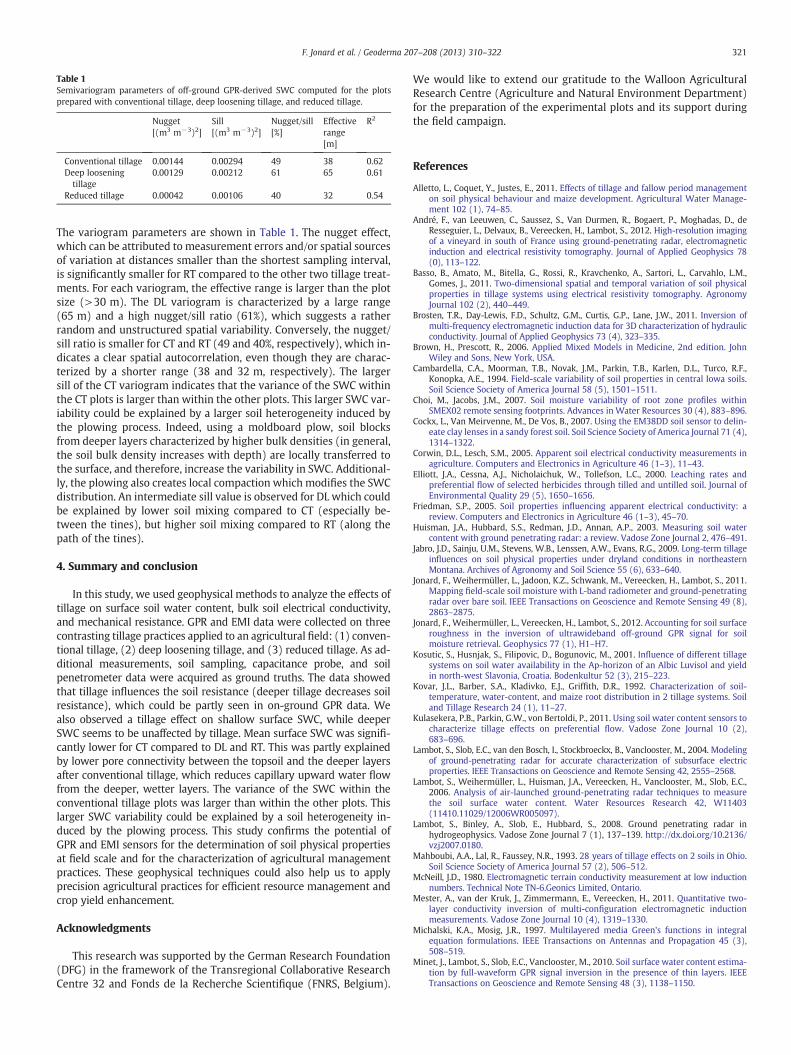
Table 1Semivariogram parameters of off-ground GPR-derived SWC computed for the plotsprepared with conventional tillage, deep loosening tillage, and reduced tillage.

Nugget[(m3 m−3)2]

Sill[(m3 m−3)2]

Nugget/sill[%]

Effectiverange[m]

R2

Conventional tillage 0.00144 0.00294 49 38 0.62Deep looseningtillage

0.00129 0.00212 61 65 0.61

Reduced tillage 0.00042 0.00106 40 32 0.54

321F. Jonard et al. / Geoderma 207–208 (2013) 310–322

The variogram parameters are shown in Table 1. The nugget effect,which can be attributed to measurement errors and/or spatial sourcesof variation at distances smaller than the shortest sampling interval,is significantly smaller for RT compared to the other two tillage treat-ments. For each variogram, the effective range is larger than the plotsize (>30 m). The DL variogram is characterized by a large range(65 m) and a high nugget/sill ratio (61%), which suggests a ratherrandom and unstructured spatial variability. Conversely, the nugget/sill ratio is smaller for CT and RT (49 and 40%, respectively), which in-dicates a clear spatial autocorrelation, even though they are charac-terized by a shorter range (38 and 32 m, respectively). The largersill of the CT variogram indicates that the variance of the SWC withinthe CT plots is larger than within the other plots. This larger SWC var-iability could be explained by a larger soil heterogeneity induced bythe plowing process. Indeed, using a moldboard plow, soil blocksfrom deeper layers characterized by higher bulk densities (in general,the soil bulk density increases with depth) are locally transferred tothe surface, and therefore, increase the variability in SWC. Additional-ly, the plowing also creates local compaction which modifies the SWCdistribution. An intermediate sill value is observed for DL which couldbe explained by lower soil mixing compared to CT (especially be-tween the tines), but higher soil mixing compared to RT (along thepath of the tines).

4. Summary and conclusion

In this study, we used geophysical methods to analyze the effects oftillage on surface soil water content, bulk soil electrical conductivity,and mechanical resistance. GPR and EMI data were collected on threecontrasting tillage practices applied to an agricultural field: (1) conven-tional tillage, (2) deep loosening tillage, and (3) reduced tillage. As ad-ditional measurements, soil sampling, capacitance probe, and soilpenetrometer data were acquired as ground truths. The data showedthat tillage influences the soil resistance (deeper tillage decreases soilresistance), which could be partly seen in on-ground GPR data. Wealso observed a tillage effect on shallow surface SWC, while deeperSWC seems to be unaffected by tillage. Mean surface SWC was signifi-cantly lower for CT compared to DL and RT. This was partly explainedby lower pore connectivity between the topsoil and the deeper layersafter conventional tillage, which reduces capillary upward water flowfrom the deeper, wetter layers. The variance of the SWC within theconventional tillage plots was larger than within the other plots. Thislarger SWC variability could be explained by a soil heterogeneity in-duced by the plowing process. This study confirms the potential ofGPR and EMI sensors for the determination of soil physical propertiesat field scale and for the characterization of agricultural managementpractices. These geophysical techniques could also help us to applyprecision agricultural practices for efficient resource management andcrop yield enhancement.

Acknowledgments

This research was supported by the German Research Foundation(DFG) in the framework of the Transregional Collaborative ResearchCentre 32 and Fonds de la Recherche Scientifique (FNRS, Belgium).

We would like to extend our gratitude to the Walloon AgriculturalResearch Centre (Agriculture and Natural Environment Department)for the preparation of the experimental plots and its support duringthe field campaign.

References

Alletto, L., Coquet, Y., Justes, E., 2011. Effects of tillage and fallow period managementon soil physical behaviour and maize development. Agricultural Water Manage-ment 102 (1), 74–85.

André, F., van Leeuwen, C., Saussez, S., Van Durmen, R., Bogaert, P., Moghadas, D., deResseguier, L., Delvaux, B., Vereecken, H., Lambot, S., 2012. High-resolution imagingof a vineyard in south of France using ground-penetrating radar, electromagneticinduction and electrical resistivity tomography. Journal of Applied Geophysics 78(0), 113–122.

Basso, B., Amato, M., Bitella, G., Rossi, R., Kravchenko, A., Sartori, L., Carvahlo, L.M.,Gomes, J., 2011. Two-dimensional spatial and temporal variation of soil physicalproperties in tillage systems using electrical resistivity tomography. AgronomyJournal 102 (2), 440–449.

Brosten, T.R., Day-Lewis, F.D., Schultz, G.M., Curtis, G.P., Lane, J.W., 2011. Inversion ofmulti-frequency electromagnetic induction data for 3D characterization of hydraulicconductivity. Journal of Applied Geophysics 73 (4), 323–335.

Brown, H., Prescott, R., 2006. Applied Mixed Models in Medicine, 2nd edition. JohnWiley and Sons, New York, USA.

Cambardella, C.A., Moorman, T.B., Novak, J.M., Parkin, T.B., Karlen, D.L., Turco, R.F.,Konopka, A.E., 1994. Field-scale variability of soil properties in central Iowa soils.Soil Science Society of America Journal 58 (5), 1501–1511.

Choi, M., Jacobs, J.M., 2007. Soil moisture variability of root zone profiles withinSMEX02 remote sensing footprints. Advances in Water Resources 30 (4), 883–896.

Cockx, L., Van Meirvenne, M., De Vos, B., 2007. Using the EM38DD soil sensor to delin-eate clay lenses in a sandy forest soil. Soil Science Society of America Journal 71 (4),1314–1322.

Corwin, D.L., Lesch, S.M., 2005. Apparent soil electrical conductivity measurements inagriculture. Computers and Electronics in Agriculture 46 (1–3), 11–43.

Elliott, J.A., Cessna, A.J., Nicholaichuk, W., Tollefson, L.C., 2000. Leaching rates andpreferential flow of selected herbicides through tilled and untilled soil. Journal ofEnvironmental Quality 29 (5), 1650–1656.

Friedman, S.P., 2005. Soil properties influencing apparent electrical conductivity: areview. Computers and Electronics in Agriculture 46 (1–3), 45–70.

Huisman, J.A., Hubbard, S.S., Redman, J.D., Annan, A.P., 2003. Measuring soil watercontent with ground penetrating radar: a review. Vadose Zone Journal 2, 476–491.

Jabro, J.D., Sainju, U.M., Stevens, W.B., Lenssen, A.W., Evans, R.G., 2009. Long-term tillageinfluences on soil physical properties under dryland conditions in northeasternMontana. Archives of Agronomy and Soil Science 55 (6), 633–640.

Jonard, F., Weihermüller, L., Jadoon, K.Z., Schwank, M., Vereecken, H., Lambot, S., 2011.Mapping field-scale soil moisture with L-band radiometer and ground-penetratingradar over bare soil. IEEE Transactions on Geoscience and Remote Sensing 49 (8),2863–2875.

Jonard, F., Weihermüller, L., Vereecken, H., Lambot, S., 2012. Accounting for soil surfaceroughness in the inversion of ultrawideband off-ground GPR signal for soilmoisture retrieval. Geophysics 77 (1), H1–H7.

Kosutic, S., Husnjak, S., Filipovic, D., Bogunovic, M., 2001. Influence of different tillagesystems on soil water availability in the Ap-horizon of an Albic Luvisol and yieldin north-west Slavonia, Croatia. Bodenkultur 52 (3), 215–223.

Kovar, J.L., Barber, S.A., Kladivko, E.J., Griffith, D.R., 1992. Characterization of soil-temperature, water-content, and maize root distribution in 2 tillage systems. Soiland Tillage Research 24 (1), 11–27.

Kulasekera, P.B., Parkin, G.W., von Bertoldi, P., 2011. Using soil water content sensors tocharacterize tillage effects on preferential flow. Vadose Zone Journal 10 (2),683–696.

Lambot, S., Slob, E.C., van den Bosch, I., Stockbroeckx, B., Vanclooster, M., 2004. Modelingof ground-penetrating radar for accurate characterization of subsurface electricproperties. IEEE Transactions on Geoscience and Remote Sensing 42, 2555–2568.

Lambot, S., Weihermüller, L., Huisman, J.A., Vereecken, H., Vanclooster, M., Slob, E.C.,2006. Analysis of air-launched ground-penetrating radar techniques to measurethe soil surface water content. Water Resources Research 42, W11403(11410.11029/12006WR005097).

Lambot, S., Binley, A., Slob, E., Hubbard, S., 2008. Ground penetrating radar inhydrogeophysics. Vadose Zone Journal 7 (1), 137–139. http://dx.doi.org/10.2136/vzj2007.0180.

Mahboubi, A.A., Lal, R., Faussey, N.R., 1993. 28 years of tillage effects on 2 soils in Ohio.Soil Science Society of America Journal 57 (2), 506–512.

McNeill, J.D., 1980. Electromagnetic terrain conductivity measurement at low inductionnumbers. Technical Note TN-6.Geonics Limited, Ontario.

Mester, A., van der Kruk, J., Zimmermann, E., Vereecken, H., 2011. Quantitative two-layer conductivity inversion of multi-configuration electromagnetic inductionmeasurements. Vadose Zone Journal 10 (4), 1319–1330.

Michalski, K.A., Mosig, J.R., 1997. Multilayered media Green's functions in integralequation formulations. IEEE Transactions on Antennas and Propagation 45 (3),508–519.

Minet, J., Lambot, S., Slob, E.C., Vanclooster, M., 2010. Soil surface water content estima-tion by full-waveform GPR signal inversion in the presence of thin layers. IEEETransactions on Geoscience and Remote Sensing 48 (3), 1138–1150.

322 F. Jonard et al. / Geoderma 207–208 (2013) 310–322

Minet, J., Bogaert, P., Vanclooster, M., Lambot, S., 2012. Validation of ground penetratingradar full-waveform inversion for field scale soil moisture mapping. Journal ofHydrology 424–425, 112–123.

Müller, M., Kurz, G., Yaramanci, U., 2009. Influence of tillage methods on soil watercontent and geophysical properties. Near Surface Geophysics 7 (1), 27–36.

Ndiaye, B., Molenat, J., Hallaire, V., Gascuel, C., Hamon, Y., 2007. Effects of agriculturalpractices on hydraulic properties and water movement in soils in Brittany(France). Soil and Tillage Research 93 (2), 251–263.

Oleschko, K., Korvin, G., Munoz, A., Velazquez, J., Miranda, M.E., Carreon, D., Flores, L.,Martinez, M., Velasquez-Valle, M., Brambila, F., Parrot, J.F., Ronquillo, G., 2008.Mapping soil fractal dimension in agricultural fields with GPR. Nonlinear Processesin Geophysics 15 (5), 711–725.

Reedy, R.C., Scanlon, B.R., 2003. Soil water content monitoring using electromagneticinduction. Journal of Geotechnical and Geoenvironmental Engineering 129 (11),1028–1039.

Richard, G., Rouveure, R., Chanzy, A., Faure, P., Chanet, M., Marionneau, A., Regnier, P.,Duval, Y., 2010. Using proximal sensors to continuously monitor agricultural soilphysical conditions for tillage management. Proximal Soil Sensing. Progress inSoil Science. Springer, Dordrecht, pp. 313–321.

Roisin, C.J.C., 2007. A multifractal approach for assessing the structural state of tilledsoils. Soil Science Society of America Journal 71 (1), 15–25.

Ryu, D., Famiglietti, J.S., 2005. Characterization of footprint-scale surface soil moisturevariability using Gaussian and beta distribution functions during the SouthernGreat Plains 1997 (SGP97) hydrology experiment. Water Resources Research 41(12), 13.

Sauer, T.J., Clothier, B.E., Daniel, T.C., 1990. Surface measurements of the hydraulic-properties of a tilled and untilled soil. Soil and Tillage Research 15 (4), 359–369.

Schwen, A., Bodner, G., Loiskandl, W., 2011a. Time-variable soil hydraulic properties innear-surface soil water simulations for different tillage methods. AgriculturalWater Management 99 (1), 42–50.

Schwen, A., Bodner, G., Scholl, P., Buchan, G.D., Loiskandl, W., 2011b. Temporal dynamicsof soil hydraulic properties and thewater-conducting porosity under different tillage.Soil and Tillage Research 113 (2), 89–98.

Slob, E., Sato, M., Olhoeft, G., 2010. Surface and borehole ground-penetrating-radardevelopments. Geophysics 75 (5), A103–A120.

Strudley, M.W., Green, T.R., Ascough, J.C., 2008. Tillage effects on soil hydraulic proper-ties in space and time: state of the science. Soil and Tillage Research 99 (1), 4–48.

Tan, C.S., Drury, C.F., Gaynor, J.D., Welacky, T.W., Reynolds, W.D., 2002. Effect of tillageand water table control on evapotranspiration, surface runoff, tile drainage and soilwater content under maize on a clay loam soil. Agricultural Water Management 54(3), 173–188.

Topp, G., Davis, J.L., Annan, A.P., 1980. Electromagnetic determination of soil watercontent: measurements in coaxial transmission lines. Water Resources Research16, 574–582.

Vereecken, H., Kamai, T., Harter, T., Kasteel, R., Hopmans, J., Vanderborght, J., 2007.Explaining soil moisture variability as a function of mean soil moisture: a stochasticunsaturated flow perspective. Geophysical Research Letters 34 (22), 6.

Zhang, S.L., Li, P.R., Yang, X.Y., Wang, Z.H., Chen, X.P., 2011. Effects of tillage and plasticmulch on soil water, growth and yield of spring-sown maize. Soil and TillageResearch 112 (1), 92–97.