Characterization of wear and tear of pH sensors exposed to

Characterization of wear and tear of pH sensors exposed to nitrified urine

Technical Report No. 7, v1.0 (TR-007-01-0)

Kito Ohmura

Dübendorf, August 30, 2018

Advisors: Dr. Kris Villez

Christian Thürlimann Marco Kipf

1

2

Contents 1. Introduction ...................................................................................................... 3

1.1. Background ................................................................................................ 3 1.2. pH measurement principle .......................................................................... 3

1.2.1. Ion-selective electrode (ISE) – general principle .................................... 3 1.2.2. Glass electrode design ......................................................................... 3 1.2.3. ISFET design ....................................................................................... 3

1.3. Objectives of this study .............................................................................. 3 2. Materials .......................................................................................................... 4

2.1. Hardware and consumables ........................................................................ 4 2.1.1. Selected pH sensors ............................................................................ 4 2.1.2. Urine nitrification reactor ...................................................................... 4 2.1.3. Calibration media ................................................................................. 5 2.1.4. Treated urine media ............................................................................. 5

3. Methods ........................................................................................................... 5 3.1. Definition of sensor quality criteria .............................................................. 5

3.1.1. Offset .................................................................................................. 5 3.1.2. Sensitivity ............................................................................................ 5 3.1.3. Response time ..................................................................................... 5

3.2. Experimental procedure .............................................................................. 6 3.2.1. Long-term exposure to nitrified urine ..................................................... 6 3.2.2. Experimental tests ................................................................................ 6

3.3. Computational procedure ............................................................................ 6 3.3.1. Offset .................................................................................................. 6 3.3.2. Sensitivity ............................................................................................ 6 3.3.3. Response time ..................................................................................... 6

4. Results ............................................................................................................ 7 4.1. Typical raw data signals ............................................................................. 7 4.2. Offset ......................................................................................................... 9 4.3. Sensitivity ................................................................................................ 10 4.4. Response time ......................................................................................... 11

4.4.1. Response time in pH 7 calibration medium .......................................... 11 4.4.2. Response time in pH 4 calibration medium .......................................... 12 4.4.3. Response time in pH 7 urine medium .................................................. 12 4.4.4. Response time in pH 4 urine medium .................................................. 13

5. Discussion and future developments ............................................................... 14 5.1. Summary of results ................................................................................... 14 5.2. Future work .............................................................................................. 14

6. Conclusions ................................................................................................... 15 7. Acknowledgements ......................................................................................... 15 8. References ..................................................................................................... 16 9. Appendices .................................................................................................... 17

A. Protocol SA1: Characterization and investigation of ageing in pH sensors ..... 17 B. Protocol SA2: Preparation of treated urine media ......................................... 20 C. Outlier: The sensor 1a measurement failure on 06.10.2016 ........................... 21

3

1. Introduction

1.1. Background Sensors play a significant role in process control. Without adequate data quality, good control or correct monitoring of process is difficult. Hence, sensors must be checked continuously and faults should be eliminated. Although there exist many methods to detect faulty sensors, our knowledge about their real-world behaviour is not adequate to assess the suitability of existing fault detection methods. In 2008, Rosén et al. defined a set of models for fault simulation. However, these models make strong, possibly unrealistic, assumptions about the assumed sensor fault symptoms.

1.2. pH measurement principle There are several pH measurements. The most popular principle for online measurement is based on an ion-selective electrode (ISE). This measurement principle is implemented most frequently in the form of a glass electrode. ISFET pH-sensors offer a popular alternative design to the glass electrode design. Other methods include the use of indicator reagents, pH test strips, and metal electrode methods. However, their applicability is limited as they require a complicated and non-automated measurement procedure (Yuqing et al., 2005). Finally, there are a number of newer methods such as the optical fibre method (Deboux et al., 1995), mass-sensitive methods (Deboux et al., 1995), conducting polymer methods (Han et al., 2001), and nano-constructed cantilever methods (Bashir et al., 2002). This study is focused on pH sensors based on the glass electrode and ISFET designs. 1.2.1. Ion-selective electrode (ISE) – general principle To apply the ISE measurement principle, the potential between a sample electrode and a reference electrode is measured. The reference electrode makes a stable reference potential by surrounding an internal element with a reference buffer solution. The reference buffer solution makes a contact with the sample solution through a junction to form an electrical circuit. With this circuit, the potential between the two electrodes is measured and the potential value is described theoretically by the Nernst equation:

.

log (1.1)

E is the total potential in mV and varies with the choice of electrodes, temperature, and pressure. The term 2.3RT/nF is called the Nernst factor (R: gas constant, F: faraday constant, n: the charge on the ion, T: temperature in degrees Kelvin) and α is the activity of the ion. Equation (1.1) can be written specifically in terms of the pH as following equation (1.2) (Westcott, 1978), where pH value is defined as equation (1.3) (Bashir et al., 2002). 0.198 ∙ (1.2) log (1.3) 1.2.2. Glass electrode design In the case of a glass electrode design, the sample electrode is made of pH sensitive glass. The glass outer surface is constructed so that the glass electrode potential is proportional to the hydrogen ion activity. 1.2.3. ISFET design The ISFET method uses an ion sensitive field effect transistor (ISFET) as a sample electrode. Hydrogen ions accumulate on the ISFET and increase the conductivity of the semiconductor base. As a result, the potential between the sample electrode and the reference electrode can be correlated with the pH dependent conductivity. The potential value is also described by the equation (1.1) and (1.2) (Bergveld, 1970).

1.3. Objectives of this study This report examines the behaviour of pH sensors under realistic circumstances and evaluates a number of existing methods to quantify the sensor’s ageing process. At the time of writing, the pH sensors were exposed to nitrified urine for a year. The specific objectives of the study are:

4

1. Quantification of sensor quality: What kind of experimental protocol is suitable to characterize the trueness, precision, and response time of a pH sensor?

2. Monitoring the ageing process of pH sensors: How does the trueness, precision and response time of a pH sensor vary as pH sensors are exposed to the harsh conditions of wastewater media.

2. Materials

2.1. Hardware and consumables 2.1.1. Selected pH sensors Five different pH sensor types are tested in this study. These types are described in Table 1. Each sensor type is manufactured by Endress+Hauser AG for use in communal wastewater treatment processes. Two sensors of each type are tested simultaneously. Each individual sensor is assigned a unique identifier (ID) consisting of a number reflecting the sensor type (1-5) and a letter reflecting the index within the pair of that type (a, b). [information removed from public release] After 6 months of operation, sensors 3a and 3b were shown to exhibit a considerably long response time in nitrified urine media. For this reason, they were replaced with sensors 5a and 5b at this time. [information removed from public release]

Table 1. Numbering and specification of sensors ID 1a 1b 2a 2b 3a 3b 4a 4b 5a 5b Type [information removed from public release] Design [information removed from public release] Liquid junction [information removed from public release] Reference system

[information removed from public release]

Installed 06.10.2016 06.10.2016 06.10.2016 06.10.2016 04.04.2017 Removed - - 29.03.2017 - 20.09.2017

2.1.2. Urine nitrification reactor During the length of the study, the pH sensors are installed into a biological reactor for urine nitrification and thereby exposed continuously to nitrified urine. The reactor is a continuous stirred tank reactor (CSTR) with a volume of 12 L. It is intermittently fed with anthropogenic urine, which is collected from urine-diverting flush toilets (NoMix toilets, Roediger Vacuum, Hanau, Germany) and waterless urinals in Eawag’s Forum Chriesbach building (Dübendorf, Switzerland). In the reactor, ammonia is converted biologically to nitrate with nitrite as an intermediate. The conversion of ammonia to nitrite is alkalinity-limited so that approximately 50% of ammonia is converted to nitrate. The pH is controlled above a minimum pH value by feeding urine whenever the pH reaches the target minimum pH. This minimum pH ranges from 6.0 to 6.8. The reactor is equipped with a bypass tube with a flow rate of 0.012 L/s. In a recent study (Fumasoli et al., 2016), the composition of men’s urine collected at EAWAG was measured. The main constituents and their recorded concentrations are listed in Table 2.

Table 2. Composition of stored urine. Extracted from (Fumasoli et al., 2016). Variable Unit Men’s urine Average ± Std. Dev pH [-] 9.0 ± 0.1 Total ammonia-N [mg/L-1] 4,140 ± 870 Nitrate-N [mg/L-1] <10 Dissolved COD [mg/L-1] 3,860 ± 870 Total inorganic C [mg/L-1] 2,080 ± 260 Total phosphate-P [mg/L-1] 242 ± 23 Potassium [mg/L-1] 1,470 ± 130 Sodium [mg/L-1] 1,760 ± 90 Sulfate [mg/L-1] 708 ± 109 Chloride [mg/L-1] 2,980 ± 440

5

2.1.3. Calibration media Calibration medium at pH 4 and pH 7 are used in this experiment to measure the sensors’ offsets, sensitivities, and dynamic responses. The product name is pH buffers CPY20 made by Endress+Hauser AG. 2.1.4. Treated urine media Treated urine medium are used to study the behaviour of pH sensors in realistic reactor conditions. The specific protocol for making the treated urine medium is added as an appendix (protocol SA2).

3. Methods

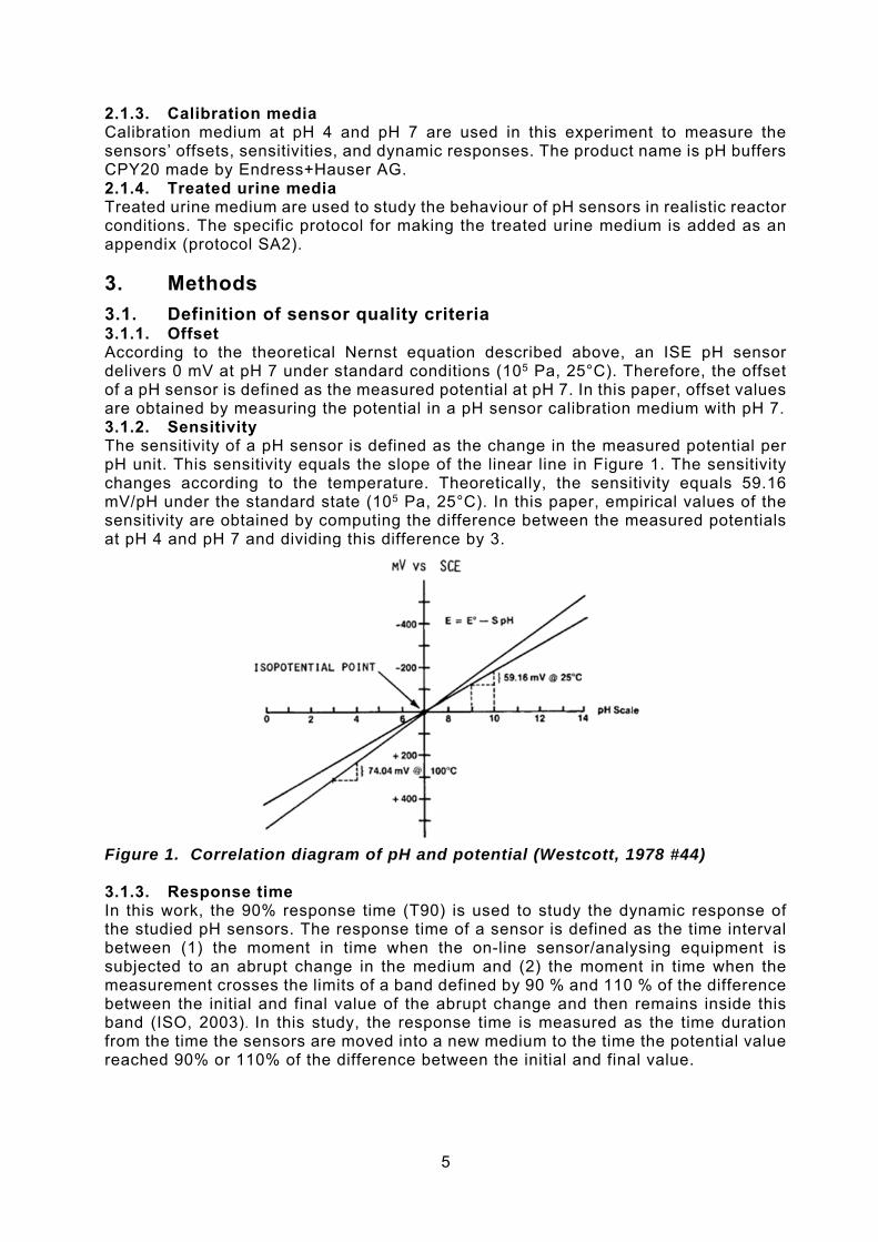
3.1. Definition of sensor quality criteria 3.1.1. Offset According to the theoretical Nernst equation described above, an ISE pH sensor delivers 0 mV at pH 7 under standard conditions (105 Pa, 25°C). Therefore, the offset of a pH sensor is defined as the measured potential at pH 7. In this paper, offset values are obtained by measuring the potential in a pH sensor calibration medium with pH 7. 3.1.2. Sensitivity The sensitivity of a pH sensor is defined as the change in the measured potential per pH unit. This sensitivity equals the slope of the linear line in Figure 1. The sensitivity changes according to the temperature. Theoretically, the sensitivity equals 59.16 mV/pH under the standard state (105 Pa, 25°C). In this paper, empirical values of the sensitivity are obtained by computing the difference between the measured potentials at pH 4 and pH 7 and dividing this difference by 3.

Figure 1. Correlation diagram of pH and potential (Westcott, 1978 #44) 3.1.3. Response time In this work, the 90% response time (T90) is used to study the dynamic response of the studied pH sensors. The response time of a sensor is defined as the time interval between (1) the moment in time when the on-line sensor/analysing equipment is subjected to an abrupt change in the medium and (2) the moment in time when the measurement crosses the limits of a band defined by 90 % and 110 % of the difference between the initial and final value of the abrupt change and then remains inside this band (ISO, 2003). In this study, the response time is measured as the time duration from the time the sensors are moved into a new medium to the time the potential value reached 90% or 110% of the difference between the initial and final value.

6

3.2. Experimental procedure 3.2.1. Long-term exposure to nitrified urine The sensors are continuously exposed to the nitrified urine medium in the urine nitrification reactor from 04.10.2016, except during execution of experimental tests. 3.2.2. Experimental tests To evaluate the criteria mentioned in previous section, the sensors are subjected to a fixed experimental protocol at regular times. The dates on which the experimental tests executed are shown in Table 3. In each experimental test, the sensors are mechanically cleaned and then immersed into treated urine media and calibration media in a specific order. The order of immersion consists of nine phases such as, phase I (tap water), phase II (treated urine media at pH 4), phase III (treated urine media at pH 7), phase IV (treated urine media at pH 4), phase V (tap water), phase VI (calibration media at pH 4), phase VII (calibration media at pH 7), phase VIII (calibration media at pH 4) and phase IX (tap water). The detailed protocol is specified as protocol SA1 in the appendix. During the experimental tests of 8th and 28th, phases II to IV and phases VI to VIII are interchanged to rule out an effect of the order of phases on the obtained results. Table 3. Dates of experimental tests executed. executed by phase II to IV and phase VI to VIII swapped Number Date [dd.mm.yyyy] Number Date [dd.mm.yyyy] Number Date [dd.mm.yyyy]

1 06.10.2016 14 29.03.2017 27 06.09.2017 2 07.10.2016 15 04.04.2017 28 20.09.2017 (*) 3 10.10.2016 16 07.04.2017 29 20.09.2017 4 12.10.2016 17 18.04.2017 30 04.10.2017 5 14.10.2016 18 03.05.2017 31 19.10.2017 6 19.10.2016 19 17.05.2017 32 01.11.2017 7 26.10.2016 20 31.05.2017 33 14.11.2017 8 11.11.2016 (*) 21 14.06.2017 34 14.12.2017 9 17.11.2016 22 28.06.2017 35 11.01.2018

10 01.12.2016 23 12.07.2017 36 08.02.2018 11 13.12.2016 24 26.07.2017 37 06.03.2018 12 22.12.2016 25 09.08.2017 13 08.02.2017 26 23.08.2017

3.3. Computational procedure The signals from the sensors, such as pH and potentials, are recorded in every second with time stamps all the time through the experiment. MATLAB® is used for all data pre-processing and computations. The programs used to obtain the criteria and all the data are included as an attachment. 3.3.1. Offset To obtain the offset, the data in the calibration medium of pH 7 (phase VII) is used. The offset of the sensor is calculated by computing the average of the last 60 data points before the time phase VIII starts. The averaged data span approximately one minute. 3.3.2. Sensitivity The difference of the potentials between calibration medium pH 4 and pH 7 equals three times sensitivity. Both data of calibration medium at pH 4 and pH 7 are obtained by taking average of the last 60 data points of phase VI and VII. 3.3.3. Response time For treated urine medium, the initial (0%) and final (100%) values are obtained by taking the average of 60 data points which are taken before approximately 60 seconds before the time next phase starts. For calibration medium, these are the values obtained before to compute the sensitivity. The initial time is manually recorded when the sensors immersed into the corresponding medium. The T90 response time is then

7

the time elapsed since this initial time when the signal enters the 90-110% band while not leaving this band anymore.

4. Results

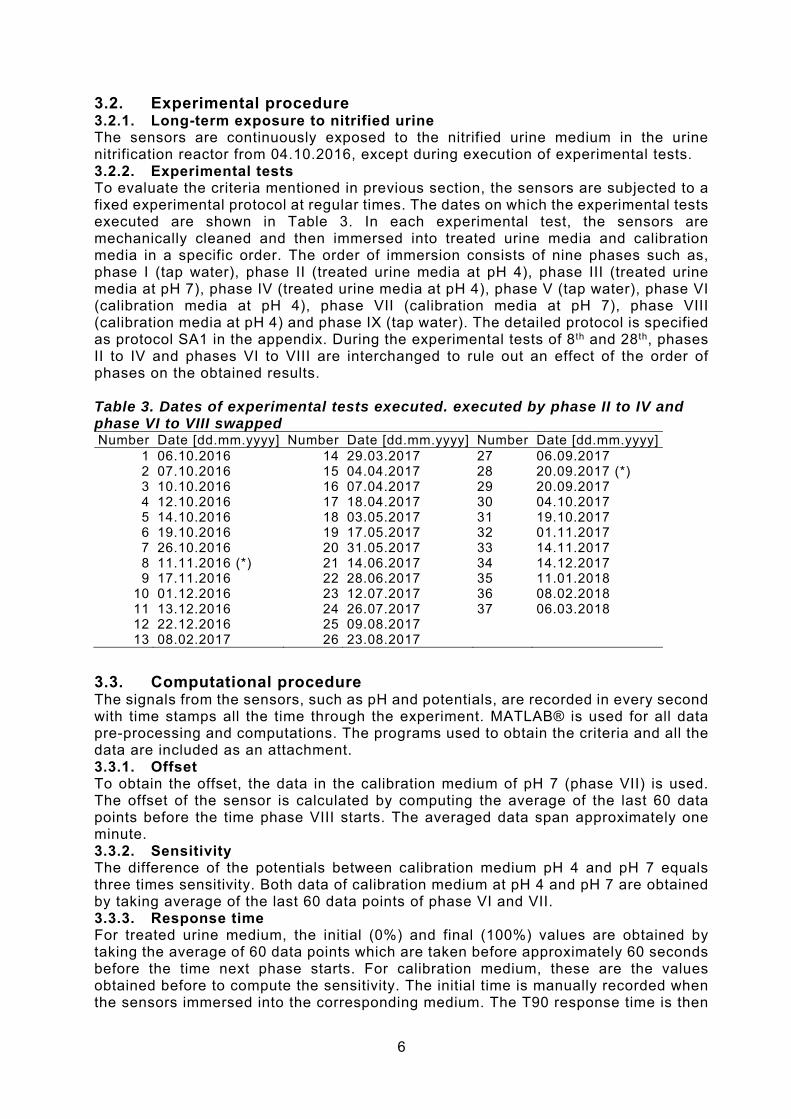
4.1. Typical raw data signals Figure 2 shows an example of how the acquired signal trends look like and the demonstration of the computer procedures. In the plot, one of the sensors (1b to 5b) displays the trend so as to follow the other sensor (1a to 5a) since we performed the experiment protocol for sensors b right after sensors a. The offset of the sensor is determined in phase VII. The sensitivity is determined by comparing the measurements in phase VII and VIII.

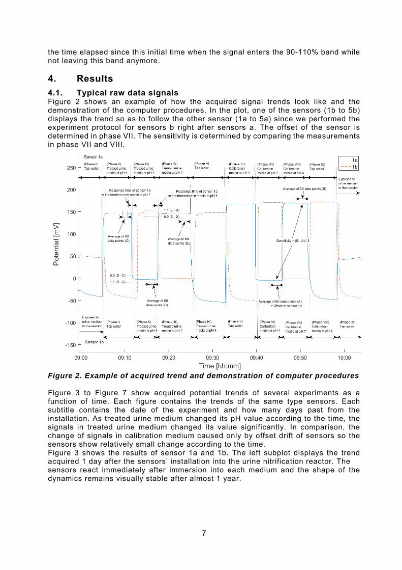
Figure 2. Example of acquired trend and demonstration of computer procedures Figure 3 to Figure 7 show acquired potential trends of several experiments as a function of time. Each figure contains the trends of the same type sensors. Each subtitle contains the date of the experiment and how many days past from the installation. As treated urine medium changed its pH value according to the time, the signals in treated urine medium changed its value significantly. In comparison, the change of signals in calibration medium caused only by offset drift of sensors so the sensors show relatively small change according to the time. Figure 3 shows the results of sensor 1a and 1b. The left subplot displays the trend acquired 1 day after the sensors’ installation into the urine nitrification reactor. The sensors react immediately after immersion into each medium and the shape of the dynamics remains visually stable after almost 1 year.

8

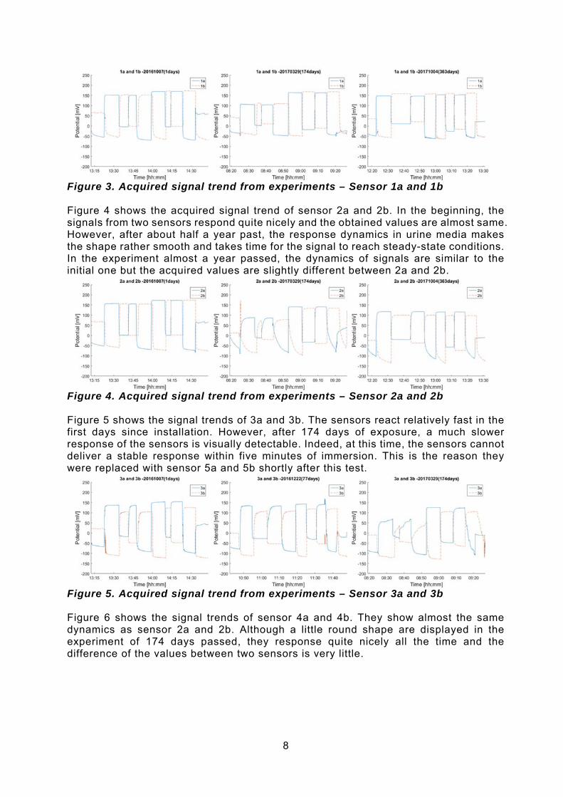
Figure 3. Acquired signal trend from experiments – Sensor 1a and 1b Figure 4 shows the acquired signal trend of sensor 2a and 2b. In the beginning, the signals from two sensors respond quite nicely and the obtained values are almost same. However, after about half a year past, the response dynamics in urine media makes the shape rather smooth and takes time for the signal to reach steady-state conditions. In the experiment almost a year passed, the dynamics of signals are similar to the initial one but the acquired values are slightly different between 2a and 2b.

Figure 4. Acquired signal trend from experiments – Sensor 2a and 2b Figure 5 shows the signal trends of 3a and 3b. The sensors react relatively fast in the first days since installation. However, after 174 days of exposure, a much slower response of the sensors is visually detectable. Indeed, at this time, the sensors cannot deliver a stable response within five minutes of immersion. This is the reason they were replaced with sensor 5a and 5b shortly after this test.

Figure 5. Acquired signal trend from experiments – Sensor 3a and 3b Figure 6 shows the signal trends of sensor 4a and 4b. They show almost the same dynamics as sensor 2a and 2b. Although a little round shape are displayed in the experiment of 174 days passed, they response quite nicely all the time and the difference of the values between two sensors is very little.

9

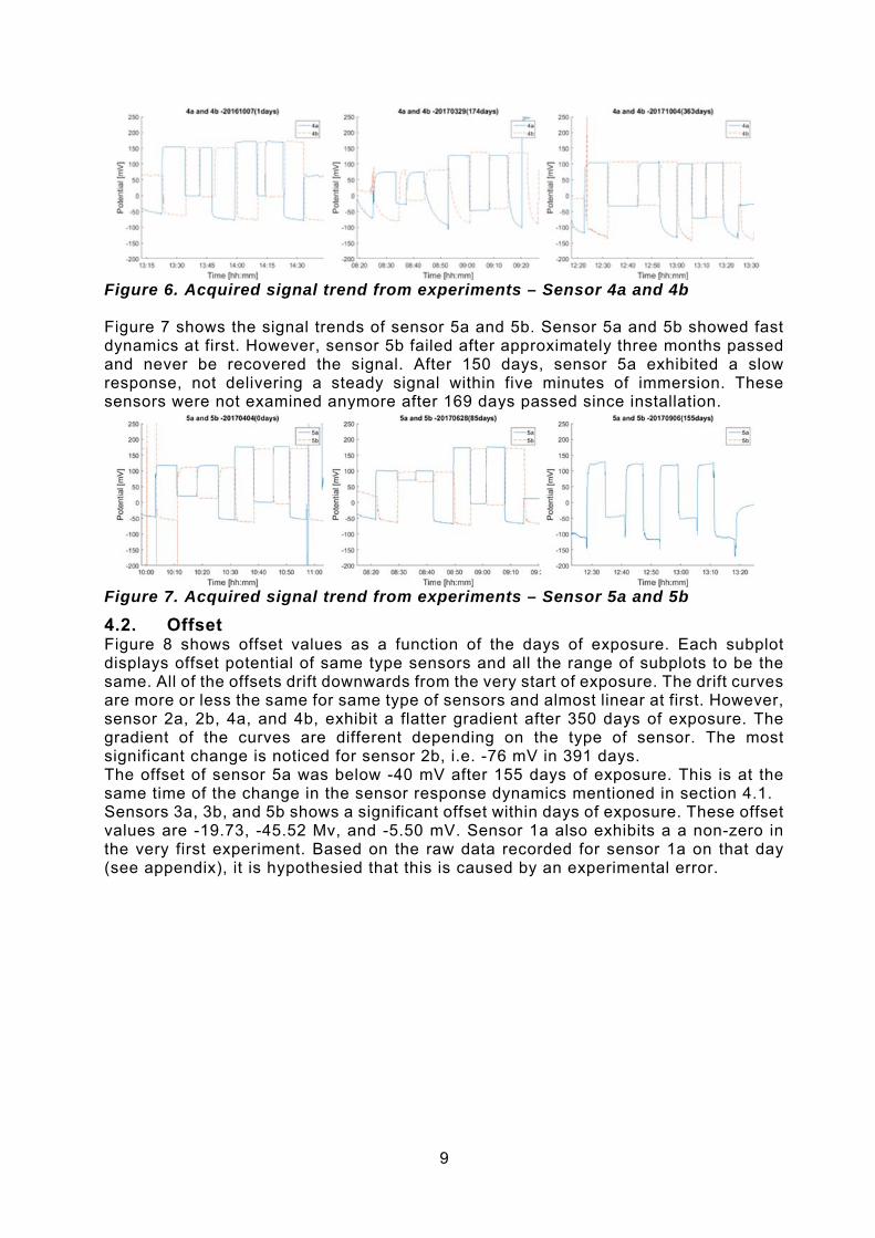
Figure 6. Acquired signal trend from experiments – Sensor 4a and 4b Figure 7 shows the signal trends of sensor 5a and 5b. Sensor 5a and 5b showed fast dynamics at first. However, sensor 5b failed after approximately three months passed and never be recovered the signal. After 150 days, sensor 5a exhibited a slow response, not delivering a steady signal within five minutes of immersion. These sensors were not examined anymore after 169 days passed since installation.

Figure 7. Acquired signal trend from experiments – Sensor 5a and 5b

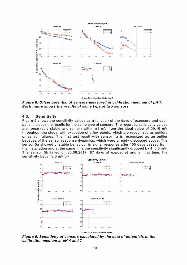
4.2. Offset Figure 8 shows offset values as a function of the days of exposure. Each subplot displays offset potential of same type sensors and all the range of subplots to be the same. All of the offsets drift downwards from the very start of exposure. The drift curves are more or less the same for same type of sensors and almost linear at first. However, sensor 2a, 2b, 4a, and 4b, exhibit a flatter gradient after 350 days of exposure. The gradient of the curves are different depending on the type of sensor. The most significant change is noticed for sensor 2b, i.e. -76 mV in 391 days. The offset of sensor 5a was below -40 mV after 155 days of exposure. This is at the same time of the change in the sensor response dynamics mentioned in section 4.1. Sensors 3a, 3b, and 5b shows a significant offset within days of exposure. These offset values are -19.73, -45.52 Mv, and -5.50 mV. Sensor 1a also exhibits a a non-zero in the very first experiment. Based on the raw data recorded for sensor 1a on that day (see appendix), it is hypothesied that this is caused by an experimental error.

10

Figure 8. Offset potential of sensors measured in calibration medium of pH 7. Each figure shows the results of same type of two sensors

4.3. Sensitivity Figure 9 shows the sensitivity values as a function of the days of exposure and each panel includes the results for the same type of sensors. The recorded sensitivity values are remarkably stable and remain within ±3 mV from the ideal value of 59.16 mV throughout the study, with exception of a few points, which are recognized as outliers or sensor failures. The first test result with sensor 1a is recognized as an outlier because of the sensor response dynamics, which were already discussed above. The sensor 5a showed unstable behaviour in signal response after 155 days passed from the installation and at the same time the sensitivity significantly dropped by 4 to 5 mV. The sensor 5b failed on 30.06.2017 (87 days of exposure) and at that time, the sensitivity became 0 mV/pH.

Figure 9. Sensitivity of sensors calculated by the data of potentials in the calibration medium at pH 4 and 7

11

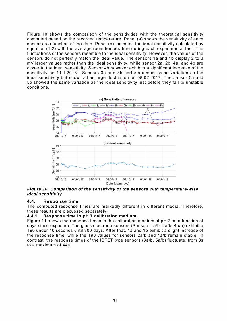
Figure 10 shows the comparison of the sensitivities with the theoretical sensitivity computed based on the recorded temperature. Panel (a) shows the sensitivity of each sensor as a function of the date. Panel (b) indicates the ideal sensitivity calculated by equation (1.2) with the average room temperature during each experimental test. The fluctuations of the sensors resemble to the ideal sensitivity. However, the values of the sensors do not perfectly match the ideal value. The sensors 1a and 1b display 2 to 3 mV larger values rather than the ideal sensitivity, while sensor 2a, 2b, 4a, and 4b are closer to the ideal sensitivity. Sensor 4b however exhibits a significant increase of the sensitivity on 11.1.2018. Sensors 3a and 3b perform almost same variation as the ideal sensitivity but show rather large fluctuation on 08.02.2017. The sensor 5a and 5b showed the same variation as the ideal sensitivity just before they fall to unstable conditions.

Figure 10. Comparison of the sensitivity of the sensors with temperature-wise ideal sensitivity

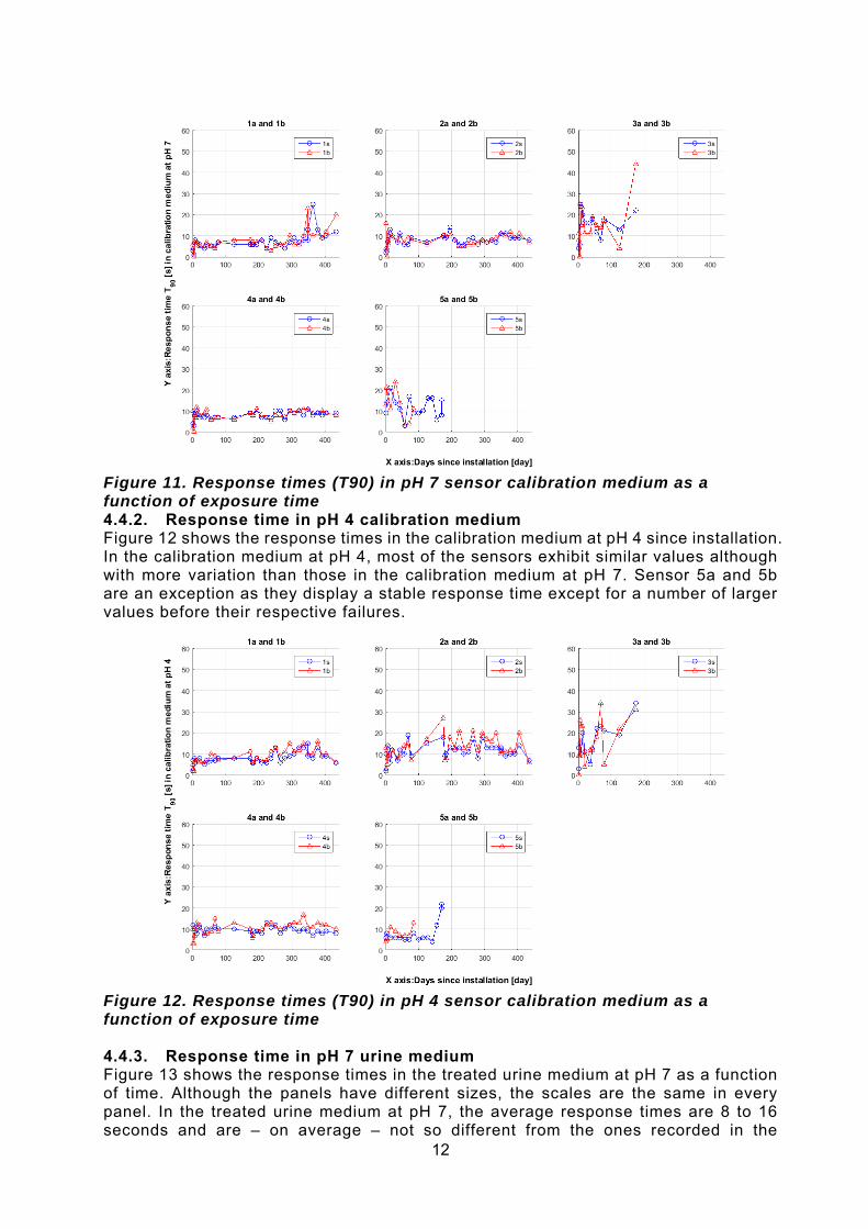
4.4. Response time The computed response times are markedly different in different media. Therefore, these results are discussed separately. 4.4.1. Response time in pH 7 calibration medium Figure 11 shows the response times in the calibration medium at pH 7 as a function of days since exposure. The glass electrode sensors (Sensors 1a/b, 2a/b, 4a/b) exhibit a T90 under 10 seconds until 300 days. After that, 1a and 1b exhibit a slight increase of the response time, while the T90 values for sensors 2a/b and 4a/b remain stable. In contrast, the response times of the ISFET type sensors (3a/b, 5a/b) fluctuate, from 3s to a maximum of 44s.

12

Figure 11. Response times (T90) in pH 7 sensor calibration medium as a function of exposure time 4.4.2. Response time in pH 4 calibration medium Figure 12 shows the response times in the calibration medium at pH 4 since installation. In the calibration medium at pH 4, most of the sensors exhibit similar values although with more variation than those in the calibration medium at pH 7. Sensor 5a and 5b are an exception as they display a stable response time except for a number of larger values before their respective failures.

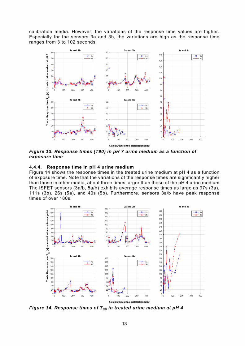
Figure 12. Response times (T90) in pH 4 sensor calibration medium as a function of exposure time 4.4.3. Response time in pH 7 urine medium Figure 13 shows the response times in the treated urine medium at pH 7 as a function of time. Although the panels have different sizes, the scales are the same in every panel. In the treated urine medium at pH 7, the average response times are 8 to 16 seconds and are – on average – not so different from the ones recorded in the

13

calibration media. However, the variations of the response time values are higher. Especially for the sensors 3a and 3b, the variations are high as the response time ranges from 3 to 102 seconds.

Figure 13. Response times (T90) in pH 7 urine medium as a function of exposure time 4.4.4. Response time in pH 4 urine medium Figure 14 shows the response times in the treated urine medium at pH 4 as a function of exposure time. Note that the variations of the response times are significantly higher than those in other media, about three times larger than those of the pH 4 urine medium. The ISFET sensors (3a/b, 5a/b) exhibits average response times as large as 97s (3a), 111s (3b), 26s (5a), and 40s (5b). Furthermore, sensors 3a/b have peak response times of over 180s.

Figure 14. Response times of in treated urine medium at pH 4

14

5. Discussion and future developments

5.1. Summary of results The first question targeted in this study concerns sensor characterization. As has been shown, the studied protocol delivers clear results for the offset and sensitivity. In contrast, the values for the response times tend to vary from test to test, making it difficult to determine whether the response times of pH sensors change over time. A possible improvement of the protocol could be obtained by including more step changes within a single test. The second question of this study concerns the quantification of the sensor ageing. The most important result is that the offsets of all studied pH sensors change continuously and from the very start of exposure to nitrified urine. This is an important observation because it can severely affect the performance of existing fault detection methods. If we wish to detect fault of sensor’s offset drift without checking offset itself, the method will likely generate many false alarms. On the other hand, if normal behaviour were to be defined with the very first data, then drift cannot be detected at all. To some surprise, the sensitivity of the pH sensors is very stable over time and the reported variations are small enough to be ignored in many practical situations. Finally, no significant changes in the response times were observed. It must be noted however that the computed response times vary a lot from one experiment to the next, therefore increasing the uncertainty about these values.

5.2. Future work The experiment in this study was designed to also enable answering the following questions:

1. Can the on-line signal of a single sensor placed in the medium be used to identify changes in trueness, precision, and response time of a pH sensor?

2. Can the on-line signals of two redundant sensors placed in the medium be used to identify changes in trueness, precision, and response time of the considered pH sensor?

3. Can changes in trueness, precision, and response time of a pH sensor be used to forecast the time to a complete failure of a sensor?

Considering that only meaningful changes in the offsets have been recorded, the above questions can be focused on drift of the offset. It is expected that a single sensor voltage signal will be difficult to relate uniquely to changes in the sensor’s offset. On the other hand, the use of two redundant sensor is promising if the redundant sensors are of a different type. Indeed, in this case the relative difference between the two mV signals could be used as a proxy for the absolute deviations due to drift. To this date, none of the commercially available sensors have failed completely. Therefore, the data cannot be used to study the forecasting of complete sensor failure. The data obtained with ISFET prototype sensors (5a/b), of which 3 have failed since their installation, may however offer some insight to this topic. The collected data also lead to the following new idea, not considered at the start of the experiment. As the changes in the offsets are typically slow and almost linear after a few months, it is hypothesized that it is possible to forecast the expected drift as soon as 2-3 months of calibration data is available. This approach, if successful, could significantly (1) reduce the maintenance costs of pH sensors in remote or low-maintenance wastewater systems or (2) increase the utility of pH sensor data in absence of frequent maintenance activities.

15

6. Conclusions In this paper, the ageing process of pH sensor exposed to nitrified urine were studied during more than one year. Through dedicated sensor tests, it is concluded that the offset of pH sensors changes (1) from the start of exposure, (2) in a continuous manner, and (3) in an almost linear fashion during the majority of the studied time window. This drift behaviour challenges existing fault detection methods as (1) it prevents the clear definition and modelling of normal behaviour and (2) one cannot assume drift to occur in a single sensor alone. The sensitivity values and response times of the sensors do not change significantly during the studied time period. An improvement of the test protocol could however deliver more precise insights into the sensor response dynamics. Based on these observations, a number of suggestions are made in the report, ranging from modification of the test protocol to possible approaches to enable fault detection in pH sensors despite the observations challenging conventional fault detection method.

7. Acknowledgements Firstly, I express deep gratitude to Dr. Kris Villez who instructed me and assisted me during this study. I would also like to thank Christian Thürlimann and Marco Kipf for helping their assistance and valuable advice. I thank Dani Iten and Stefan Vogel from Endress+Hauser for their valuable advice and input to this study. This study was made possible thanks to financial support from Toshiba, Tokyo, Japan.

16

8. References Bashir, R., Hilt, J. Z., Elibol, O., Gupta, A., & Peppas, N. A. (2002). Micromechanical

cantilever as an ultrasensitive pH microsensor. Applied Physics Letters, 81(16), 3091–3093.

Bergveld, P. (1970). Development of an Ion-Sensitive Solid-State Device for Neurophysiological Measurements. IEEE Transactions on Biomedical Engineering, BME-17(1), 70–71.

Deboux, B. J.-C., Lewis, E., Scully, P. J., & Edwards, R. (1995). A novel technique for optical fiber pH sensing based on methylene blue adsorption. Journal of Lightwave Technology, 13(7), 1407–1414.

Fumasoli, A., Etter, B., Sterkele, B., Morgenroth, E., & Udert, K. M. (2016). Operating a pilot-scale nitrification/distillation plant for complete nutrient recovery from urine. Water Science and Technology, 73(1), 215–222.

Han, W.-S., Park, M.-Y., Cho, D.-H., Hong, T.-K., Lee, D.-H., Park, J.-M., & Chung, K.-C. (2001). The Behavior of a Poly(aniline) Solid Contact pH Selective Electrode Based on N, N, N’,N’-Tetrabenzylethanediamine Ionophore. Analytical Sciences, 17(6), 727–732.

ISO. (2003). Water quality — On-line sensors/analysing equipment for water — Specifications and performance tests. Reference Number ISO, 15839(15839).

Rosén, C., Jeppsson, U., Rieger, L., & Vanrolleghem, P. A. (2008). Adding realism to simulated sensors and actuators. Water Science & Technology, 57(3), 337.

Westcott, C. C. (1978). PH measurements. Academic Press. Yuqing, M., Jianrong, C., & Keming, F. (2005). New technology for the detection of

pH. Journal of Biochemical and Biophysical Methods, 63(1), 1–9.

17

9. Appendices

A. Protocol SA1: Characterization and investigation of ageing in pH sensors

Objective

The operation and repeated testing of pH sensors placed in the same medium is executed over a long period to investigate following questions:

Sensor characterization: What kind of experimental protocol is necessary to characterize the trueness, precision, and response time of a pH sensor?

Sensor ageing: How does the trueness, precision and response time of a pH sensor change over time?

Online diagnosis: o Can the on-line signal of a single sensor placed in the medium be used

to estimate trueness, precision, and response time of a pH sensor? o Can the on-line signals of two redundant sensors placed in the medium

be used to estimate trueness, precision, and response time of the considered pH sensors?

Prognosis: Can changes in trueness, precision, and response time of a pH sensor be used to predict the complete failure of a sensor?

Materials

pH Sensors 5 x Medium (A: Tap water, B:Treated urine at pH 4, C:Treated urine at pH 7,

D:Calibration media at pH 4, E: Calibration media at pH 7) 5 x Vessels for medium 4 x Magnet stirrers 10 x Magnets

Materials preparation

pH Sensors o Acquire sensors from manufacturer. o Install sensors so that data is collected in a 1 second sampling interval. o Make sure temperature, pH, and measured voltage are recorded. o The sensors stay in their packaging without any calibration from the

delivery. Pumping loop

o Install and test the pumping loop which pumps reactor liquor of a urine nitrification reactor through the sensor test tube.

Media o Tap water (A): Collect tap water from a tap in the experimental hall at

EAWAG. o Treated urine medium (B and C) (See Protocol SA2) o Calibration medium (D and E): Buy calibration medium from manufacturer.

Experiment steps Execute the following procedure repeatedly over time to achieve the objectives.

1. Pour each medium to corresponding vessels (vessel A: Tap water, B:Treated urine at pH 4, C:Treated urine at pH 7, D:Calibration media at pH 4, E: Calibration media at pH 7) and put a pair of magnets into each vessels.

2. Move sensors from the reactor to the vessel A (Phase I) a. Place the vessel A on a pair of magnet stirrers and ensure good mixing. b. Take sensors out of the reactor

18

c. Clean sensors with tap water and a soft sponge d. Immerse the sensors into the media in the vessel A, and record the time

in the lab-journal. e. Wait 5 minutes

3. Move sensors from vessel A to B (Phase II) a. Place the vessel B on a pair of magnet stirrers and ensure good mixing. b. Take the sensors out of the vessel A. c. Shake them in the air and drop most of the solution on the sensors. d. Immerse the sensors into the media in the vessel B, and record the time


4. Move sensors from vessel B to C (Phase III) a. Place the vessel C on a pair of magnet stirrers and ensure good mixing. b. Take the sensors out of the vessel B. c. Shake them in the air and drop most of the solution on the sensors. d. Immerse the sensors into the media in the vessel C, and record the time


5. Move sensors from vessel C to B (Phase IV) a. Place the vessel B on a pair of magnet stirrers and ensure good mixing. b. Take the sensors out of the vessel C. c. Shake them in the air and drop most of the solution on the sensors. d. Immerse the sensors into the media in the vessel B, and record the time


6. Move sensors from vessel B to A (Phase V) a. Place the vessel A on a pair of magnet stirrers and ensure good mixing. b. Take the sensors out of the vessel C. c. Shake them in the air and drop most of the solution on the sensors. d. Immerse the sensors into the media in the vessel A, and record the time


7. Move sensors from vessel A to D (Phase VI) a. Place the vessel D on a pair of magnet stirrers and ensure good mixing. b. Take the sensors out of the vessel A. c. Shake them in the air and drop most of the solution on the sensors. d. Immerse the sensors into the media in the vessel D, and record the time


8. Move sensors from vessel D to E (Phase VII) a. Place the vessel E on a pair of magnet stirrers and ensure good mixing. b. Take the sensors out of the vessel D. c. Shake them in the air and drop most of the solution on the sensors. d. Immerse the sensors into the media in the vessel E, and record the time


9. Move sensors from vessel E to D (Phase VIII) a. Place the vessel D on a pair of magnet stirrers and ensure good mixing. b. Take the sensors out of the vessel E. c. Shake them in the air and drop most of the solution on the sensors. d. Immerse the sensors into the media in the vessel D, and record the time


10. Move sensors from vessel D to A (Phase IX) a. Place the vessel A on a pair of magnet stirrers and ensure good mixing. b. Take the sensors out of the vessel D.

19

c. Shake them in the air and drop most of the solution on the sensors. d. Immerse the sensors into the media in the vessel A, and record the time


11. Move sensors from the vessel A to the reactor a. Take sensors out of the vessel A b. Clean sensors with tap water and a soft sponge c. Place the sensors back to the reactor

12. Pour each medium back to the storage containers 13. Pour each medium back to the storage containers. 14. Tidy up instruments

20

B. Protocol SA2: Preparation of treated urine media Objective Prepare treated urine media used for pH sensor experiment described in Protocol SA1. Materials

5 to 6 L of nitrified urine (collect them from the urine reactor) Centrifuge machine 2x centrifugation container 2x 2L-Schottglasses Autoclave machine Magnet stirrer and magnet 50ml of 2M HCL 50ml of 2M NaOH Pipette (0.2 to 2ml) Calibrated pH probe (conditioned to nitrified urine)

Preparation steps

1. Collect 5 to 6 L of nitrified urine and fill them in the two of centrifuge container equally

2. Centrifuge all the urine to remove all particles. (repeat centrifugation if particles are not fully sedimented)

3. Take supernatant and fill 2x 2L-Schottglasses with it. Waste the sedimented particles.

4. Autoclave the two 2L-Schottglasses. 5. Label the 2L-Schottglases with bottle 1 and bottle 2. 6. Put the bottle 1 on a magnetic stirrer and add a magnet. Take the calibrated pH

probe and put it in bottle 1. 7. Adjust pH of the medium in the bottle 1 with 2M HCL to a pH of 4 (1ml additions

of HCL). Expect to start around pH 6. 8. After reaching pH 4, take the magnet and the pH probe out. Clean them with

distilled water and close the bottle 1. 9. Put the bottle 2 on the magnetic stirrer and add a magnet. Take a calibrated pH

probe and put it in the bottle 2. 10. Adjust pH of the medium in the bottle 2 with 2M NaOH to a pH of 7 (1ml additions

of NaOH). Clean them with distilled water and close the bottle again. 11. After reaching pH 7, take the magnet and the pH probe out. Clean them with

distilled water and close the bottle 2. 12. Tidy up all the instruments.

21

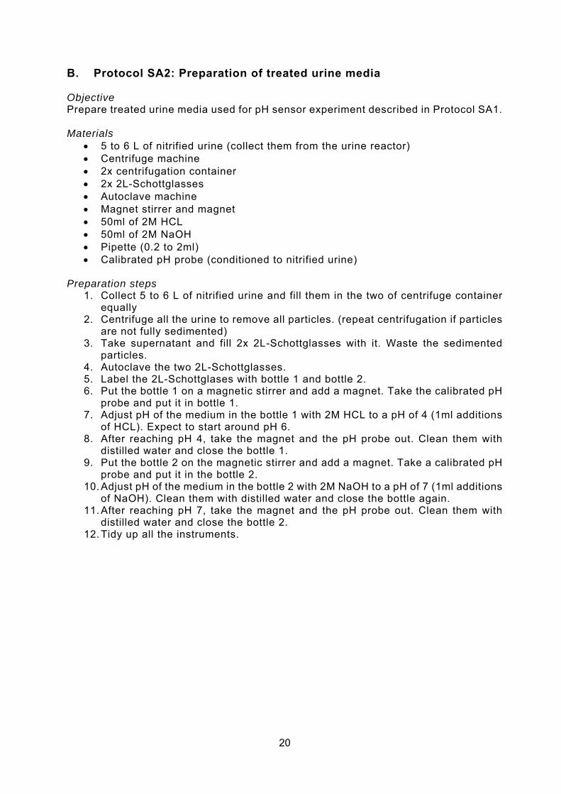
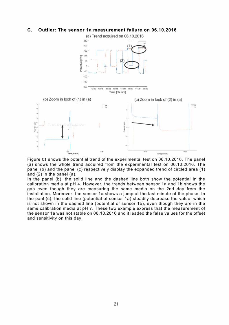
C. Outlier: The sensor 1a measurement failure on 06.10.2016

Figure C1 shows the potential trend of the experimental test on 06.10.2016. The panel (a) shows the whole trend acquired from the experimental test on 06.10.2016. The panel (b) and the panel (c) respectively display the expanded trend of circled area (1) and (2) in the panel (a). In the panel (b), the solid line and the dashed line both show the potential in the calibration media at pH 4. However, the trends between sensor 1a and 1b shows the gap even though they are measuring the same media on the 2nd day from the installation. Moreover, the sensor 1a shows a jump at the last minute of the phase. In the panl (c), the solid line (potential of sensor 1a) steadily decrease the value, which is not shown in the dashed line (potential of sensor 1b), even though they are in the same calibration media at pH 7. These two example express that the measurement of the sensor 1a was not stable on 06.10.2016 and it leaded the false values for the offset and sensitivity on this day.

22

Figure C1. The trend on 06.10.2016

Documents

Characterization of wear and tear of pH sensors exposed to