Characterizing the relationship between basic calcium phosphate particulates in the knee

joint and the frictional coefficient of articular cartilage in the intact rat knee.

Senior Honors Thesis

Departments of Mechanical Engineering and Orthopaedics

Charlotte Morgan

Advisors:

Dr. Bruce Beynnon

Dr. Maria Roemhildt

Dr. Rachael Oldinski

2

Table of Contents

Abstract 3

Introduction 3

Apparatus 6

Methods 9

Results 12

Discussion and Conclusions 17

Acknowledgements 18

References 19

Appendix I: SolidWorks Drawings 22

Appendix II: MATLAB Code 26

Appendix III: Data Processing Plots 44

3

Abstract

In order to examine the role of calcium phosphate particulates in the development of joint

degeneration, a pendulum apparatus for evaluating the whole-joint coefficient of friction of intact

knees using the rat model was designed, constructed, and evaluated. The femur is mounted to

the apparatus at a fixed angle, and a weighted pendulum is affixed to the tibia such that its

weight places the joint in compression. The pendulum is displaced, and then allowed to oscillate

freely until it returns to rest. The oscillation of the pendulum is recorded using an optical

tracking system. A decay function is fitted to the oscillation in MATLAB, and the coefficient of

friction is derived from this function. An initial sample population (n = 2 limbs) of pilot

specimens was prepared, and the coefficient of friction of each specimen was evaluated in its

naïve state, and following particulate injections at 0, 1, 10, and 100 mg/mL concentrations. The

coefficient of friction of each specimen was evaluated after each injection. The 0 mg/mL

treatment (phosphate buffered saline only) was found to have no statistically significant effect on

coefficient of friction (p = 131); all other treatments investigated were found to cause statistically

significant increases in coefficient of friction (p < 0.001). Based upon these data, a

physiologically plausible treatment of 100 μL of 1 mg/mL suspension was selected for the main

study. A sample population (n = 6 limbs) of specimens was prepared, and the coefficient of

friction of each specimen was evaluated in its naïve state and after sham (saline) and loaded

(1 mg/mL) treatments. The sham treatment was found to have no statistically significant effect

(p = 0.367), while the loaded treatment was found to cause a 31% increase in coefficient of

friction (p = 0.039).

Introduction

Osteoarthritis (OA) of the knee affects over 9 million adults over age 60 in the United States

alone.21

OA is a painful condition characterized by wear, degradation, and loss of joint cartilage,

and can seriously impact physical ability and quality of life. Treatment of OA is complicated by

the fact that once damaged, cartilage heals poorly. Thus, prevention and mitigation of damage

are critical. Improved understanding of the numerous risk factors associated with the

development and progression of OA may eventually lead to better prediction, earlier

intervention, novel therapies, and better overall care. Characterizing the effects of basic calcium

phosphates on joint friction in the rat model may lead to a more complete understanding of their

relationship to OA in humans.

The formation of mineralized cysts within the matrix of articular cartilage is a form of cartilage

degradation associated with aging and OA.13

The deposition of basic calcium phosphates in

articular cartilage has been associated with aging, decreased joint function, and severity of

osteoarthritis in humans.8,9

Common mineral species found in cystic deposits include calcium

pyrophosphate (associated with pseudogout) and a variety of other calcium phosphate species,

including carbonate-substituted hydroxyapatite, tricalcium phosphates, octacalcium phosphate,

and whitlockite; these species are collectively referred to as basic calcium phosphates (BCPs).18

As cartilage is worn away at the articulating surface of the joint or cysts increase in size, these

cysts become exposed and ultimately rupture, releasing their contents into the synovial fluid.

Cystic BCP deposits analogous to those found in human joints are also common in the joints of

mature Sprague-Dawley rats.18

4

Little is currently known about the tribological effects of cartilage mineralization. The

phenomenon has been characterized and mechanical analyses of affected tissue have been

performed in the rat model, but the mechanisms of cyst formation and the tribological effects of

cyst rupture remain unknown.18

In the human hip joint, the degree of BCP calcification has been

found to correlate to clinical symptoms and histological markers of OA.8 Calcification has been

linked to both aging and OA, and mineral particulates and wear debris have been found to

contribute to inflammation and degeneration. It is possible that the presence of BCPs in the joint

capsule contributes to OA through cartilage abrasion, as well as by inducing inflammation.13

From a mechanical perspective, the introduction of hard particulate matter into the lubricating

fluid of any joint or bearing alters the interaction between contact surfaces, typically resulting in

an increase in friction and ultimately in abrasive wear. However, the specific relationship

between synovial BCPs and joint friction is currently unknown.

A variety of arthropathies are linked to the presence of mineral crystals in the joints.

Pyrophosphate arthropathies such as calcium pyrophosphate dihydrate disease (CPPD) provide

some insight into the possible effects of intracapsular mineral particulates. In CPPD, the

presence of calcium pyrophosphate (CPP) in the synovial fluid leads to swelling and

inflammation.4 While some crystalline arthropathies, such as gout, are caused by the formation

of crystals in the joint fluid and surrounding soft tissues, CPPD is caused by the release of CPP

into the joint capsule from cystic formations in the connective tissue, mechanically similar to the

rupture of BCP cysts in OA. The in-vivo introduction of CPP into the synovial fluid of the knee

joints of rabbits with preexisting induced OA has been found to increase the severity of the

condition, suggesting that the presence of intracapsular particulates can exacerbate cartilage wear

and inflammation.4

Rats are widely used as model organisms in OA research, as their small size makes them easy

and cost-effective to keep, and their rapid maturation allows efficient longitudinal study.12

However, their small size complicates surgical modeling procedures and specimen manipulation,

and provides limited amounts of tissue for subsequent analysis. Due to these size constraints,

pendulum testing is the preferred method for evaluating joint friction in small-animal models.1

Other commonly-used methods of evaluating friction, such as pin-on-disk, pin-on-plate, and

cartilage plug analysis, examine the interaction between a metal or glass instrument and a

cartilage sample. In rats, mice, and other small animals, however, these methods are impractical

or impossible due to the difficulty of excising and manipulating cartilage samples on such a

small scale. For example, the thickness of the articular cartilage layer in the rat knee is

approximately 300 μm.18

By utilizing the whole, intact knee joint, the pendulum method

eliminates the need to excise and manipulate such miniscule samples.

The measured coefficient of friction of a material also varies depending upon the lubricant used

and the material with which it is interacting. Data obtained via this method reflect the frictional

properties of synovially-lubricated cartilage-on-cartilage contact between geometrically

compatible articular surfaces over an anatomically appropriate range of motion—that is to say,

the data reflect the properties of the whole joint under conditions similar to those which exist in

vivo. Furthermore, the pendulum method preserves the natural anatomical structures of the joint,

ensuring that the articulating surfaces interact with one another much as they would in vivo. A

further advantage of the pendulum method for this area of inquiry is that an intact joint capsule

5

can contain and retain fluids, allowing the introduction of a fluid particulate suspension into the

joint space in order to simulate BCP release due to cyst rupture.

The small-animal pendulum testing methodology described by Drewniak et al. uses the whole

joint and adjacent bones.2,3

The femur is mounted to the apparatus at a fixed angle; a weighted

pendulum is affixed to the tibia such that its weight places the joint in compression. The flexion

angle of the joint when the pendulum is at rest is chosen to approximate the mean flexion angle

of the knee joint during the gait cycle in vivo.2,3

In rats, this angle is ~67°.5,6

Pendulum weight

is based upon percentage of mean specimen bodyweight, representing ordinary weight-bearing

limb use. For skeletally mature Sprague-Dawley rat specimens with average body mass of

approximately 600 g, the pendulum mass should be 300 g, or approximately 50% bodyweight,

reflecting the mean joint loading during gait.22

Pendulum length is chosen to yield a pendulum

frequency approximating the flexion frequency of a continuous walking gait; in rats, this

frequency is ~1 Hz.1,22

The pendulum is displaced by an angle equal to half the mean range of

motion during gait—12° in rats—then released and allowed to oscillate freely until it returns to

rest.5,6,22

The oscillation of the pendulum is tracked using an optical tracking system, and the

coefficient of friction is determined by analysis of the decay envelope of the oscillation.

The model most commonly used to derive coefficient of friction from pendulum data is the

Stanton, or linear, fit. This model approximates the decay of the oscillation as a linear function,

and derives a linear coefficient of friction μ from the slope of the line as

μ = lm / 4r

where l is the distance the fulcrum to the center of mass of the pendulum, m is the slope of the

linear-fit decay function, and r is the epicondylar radius.1 This linear approach does not

accurately reflect the curved profile of the decay envelope, however, and does not account for

viscous damping effects due to soft tissues or air resistance. A second approach is to fit a

function with both exponential and linear terms to the data to obtain a coefficient of viscous

damping c and a coefficient of friction u as

u = 4δπ2Iθ0 / mgrT

2 and c = 4jπI / T

where δ is derived from a coefficient of the model, j = cT / 4πI, θ0 is the angular displacement at

cycle 0, T is the time between cycles, I is the moment of inertia of the pendulum, m is the mass

of the pendulum, g is the gravitational constant, and r is the epicondylar radius.25

A comparative study applied both Stanton (“linear”) and combined linear-exponential

(“combination”) decay models to the same experimental data, and concluded that although the

combination model fits the experimental data more closely and accounts for viscous damping,

and thus more accurately reflects the behavior of the specimen, the linear model has greater

measurement precision.2 Furthermore, the linear model has been widely used, and thus linear fit

analyses are more directly comparable to existing research.2 Due to the differing advantages of

both methods, however, it is prudent to analyze experimental data using both methods.

6

The aims of this research are a) to develop an experimental apparatus for the purpose of

determining the whole-joint coefficient of friction of a specimen in vitro, and b) to determine

whether the presence of basic calcium phosphate particulate in the joint capsule has a significant

effect upon whole-joint coefficient of friction. The primary hypothesis is that the whole-joint

coefficient of friction will increase with the introduction of basic calcium phosphate particulate

into the intracapsular space.

Apparatus

Pendulum Device

Figure I: Full Pendulum Device with Specimen and Trigger Bar

The pendulum device consists of three main elements: the frame, the mounting block, and the

pendulum. The frame is constructed of 25 mm (1”) square T-slotted extruded aluminum tubing.

T-slotted tubing was selected for its strength, light weight, and ease of assembly. Because of the

modular nature of the tubing, the frame can be fully disassembled for storage, and is easily

reconfigurable to accommodate additions and modifications. A wide rectangular footprint

provides stability. The height of the frame can accommodate pendulum of up to 45 cm in length,

making it possible to test larger specimens or at lower frequencies if desired. The two front

upright members, located at opposite sides of the base, create an uninterrupted viewing window

within which the pendulum can be optically tracked without marker occlusion. The single rear

upright member and associated crosspieces support the mounting block. The entire frame is

painted matte black to minimize reflective interference with the optical tracking system.

7

Figure II: Mounting Block with Specimen and Pendulum, Two Views

The mounting block is fabricated of high-density polyethylene. It is removable, and can be

replaced with another block or other mounting platform, allowing the frame to be used with

larger or smaller model organisms. A removable angle block sets the specimen mounting angle;

this block can be replaced to allow reuse of the mounting block with other similarly-sized model

organisms and different ranges of motion. Two set screws fix the position of the specimen when

mounted in the block. An acrylic viewing window allows visual observation of the specimen

when mounted and aids in orientation during mounting. A reservoir allows the specimen to be

immersed in saline solution or cell culture medium to maintain hydration during extended

testing. The exterior of the mounting block is painted matte black to minimize reflective

interference with the optical tracking system; the viewing window and interior are unpainted for

ease of observation.

The pendulum is fabricated of aluminum stock, and has an overall length of 28 cm below the

upper crosspiece. A milled socket in the upper crosspiece fits the 11 mm (7/16”) potting tube

used for the tibial segments. Pairs of holes in the side pieces allow adjustment of the lower

crosspiece position (and hence the center of mass) by increments of 10 mm. Holes in the lower

crosspiece allow the addition of plates to adjust the mass, and a bearing on the lower crosspiece

interfaces with a linear actuation system to allow cyclic loading of the specimen. The pendulum

is painted matte black to minimize reflective interference with the optical tracking system. Four

4 mm self-adhesive retroreflective markers (NaturalPoint, Corvallis OR) are affixed

noncollinearly to one side of the pendulum, allowing it to be defined as a rigid body by the

optical tracking software.

The trigger bar is an auxiliary tool used to uniformly and reproducibly deflect the mounted

specimen for motion trials. It consists of two telescoping lengths of square aluminum tubing

with a slot and thumbscrew for fixing the length. Crosspieces at either end allow one end to be

placed flush with an element of the frame base, while the other end catches the bottom of the

pendulum. The deflection angle is set by adjusting the length of the trigger bar such that it

deflects the pendulum to the desired degree. Pendulum deflection is confirmed visually using a

goniometer, and the length of the trigger bar is fixed.

8

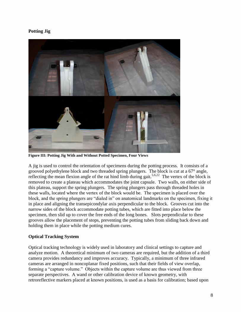
Potting Jig

Figure III: Potting Jig With and Without Potted Specimen, Four Views

A jig is used to control the orientation of specimens during the potting process. It consists of a

grooved polyethylene block and two threaded spring plungers. The block is cut at a 67° angle,

reflecting the mean flexion angle of the rat hind limb during gait.5,6,22

The vertex of the block is

removed to create a plateau which accommodates the joint capsule. Two walls, on either side of

this plateau, support the spring plungers. The spring plungers pass through threaded holes in

these walls, located where the vertex of the block would be. The specimen is placed over the

block, and the spring plungers are “dialed in” on anatomical landmarks on the specimen, fixing it

in place and aligning the transepicondylar axis perpendicular to the block. Grooves cut into the

narrow sides of the block accommodate potting tubes, which are fitted into place below the

specimen, then slid up to cover the free ends of the long bones. Slots perpendicular to these

grooves allow the placement of stops, preventing the potting tubes from sliding back down and

holding them in place while the potting medium cures.

Optical Tracking System

Optical tracking technology is widely used in laboratory and clinical settings to capture and

analyze motion. A theoretical minimum of two cameras are required, but the addition of a third

camera provides redundancy and improves accuracy. Typically, a minimum of three infrared

cameras are arranged in noncoplanar fixed positions, such that their fields of view overlap,

forming a “capture volume.” Objects within the capture volume are thus viewed from three

separate perspectives. A wand or other calibration device of known geometry, with

retroreflective markers placed at known positions, is used as a basis for calibration; based upon

9

the observed relative position of the markers and the geometry of the calibration tool, a spatial

coordinate system is derived. Retroreflective markers are applied to the objects to be tracked,

and their motion within the capture volume is recorded. A number of tracking systems were

evaluated, and OptiTrack Flex 13 cameras with compatible Tracking Tools software package

(NaturalPoint, Corvallis OR) were selected based on the high rated translational accuracy (0.1

mm) and the relatively low cost of the system. A calibration tool, ground plane tool (used to

define axes within capture volume), and self-adhesive retroreflective markers were also obtained

from NaturalPoint.

Methods

Optical Tracking System

Cameras were mounted on small tripods for stability and arrayed noncoplanarly on a bench ~5

feet from experimental apparatus, and all associated cables were plugged in and arranged to

prevent future disturbance of camera position. Individual camera orientation was adjusted such

that the capture volume encompassed a space sufficient to accommodate the experimental

apparatus. Using the motion tracking software package (Tracking Tools, NaturalPoint, Corvallis

OR), a full camera calibration was run. Wanding was performed uniformly and methodically

throughout the capture volume. The frame of the pendulum apparatus was then placed on the

bench, and more intensive wanding was performed within the volume defined by the frame,

where accuracy is most critical. After calibration, the critical region of the capture volume was

evaluated using the calibration wand. Overall wand error within the frame was found to be less

than 0.1% (less than 0.25 mm). The ground plane tool (NaturalPoint) was placed on the bench

and aligned with the frame, and the ground plane was set in Tracking Tools and the calibration

was saved for later use. The ground plane tool was then removed to minimize unnecessary

marker capture during trials.

Specimen Preparation

Hind limbs were disarticulated at the hip and ankle joints, and the soft tissues were dissected

away to expose the joint capsule and the medial and lateral collateral ligaments. A small portion

of the quadriceps femoris was preserved in order to anchor the patellar tendon and and maintain

the integrity of the joint capsule. On each specimen, a hole was drilled axially through the distal

end of the tibia, and a fine wire approximately 40 mm in length (“tibial pin”) was inserted.

Tibial pins were fixed in place with a fast-curing cyanoacrylate adhesive, and then visually

aligned with the central axis of the tibiofibular segment. Prepared specimens were wrapped in

saline-soaked gauze to prevent dehydration during storage.

Prepared and thawed specimens were patted dry, and the femoral insertion points of the medial

and lateral collateral ligaments were visually identified and marked with a dot of ink. Location

of insertion points was then confirmed by probing for non-visible bony landmarks (“divots”)

using fine-tipped dissecting forceps. Specimens were placed over potting jig in correct

orientation relative to grooves, and spring plungers were “dialed in” on landmark points, fixing

the orientation of the specimen relative to the jig, such that the transepicondylar axis of the

10

specimen was oriented perpendicular to the grooves, and the long axis of the tibiofibular segment

was parallel to the grooves.

Potting tubes (11 mm (7/16”) square for tibia, 19 mm (3/4") square for femur, 35 mm length)

were sealed at one end with masking tape. Tape was folded down onto the sides of the tube for

adhesion, and any excess tape where the tube interfaces with the potting jig was trimmed away

with a razor blade. The center of the sealed end of the tibial tube was geometrically located, and

a small puncture was made. The tibial tube was then fitted into the tibial groove and the free end

of the tibial pin was aligned such that it passes through the center of the sealed end. The tibial

tube was then slid up to cover the free end of the tibiofibular segment, and fixed in place with a

stop. The femoral tube was applied to the free end of the femoral segment and fixed in place in

the same manner, but without controlling axial alignment.

The potting jig was placed under a fume hood (or other adequate ventilation), and the base was

propped up at an angle of ~35 degrees, such that the tibial tube was approximately vertical. A

small batch (~2.5 g solid) of polymethylmethacrylate (PMMA) cement (Acraweld Repair Resin

and Self Cure Acrylic Liquid, Henry Schein #101-1105 and #101-7550) was prepared at a ratio

of 1 g solid to 1 mL liquid, and injected into the tibial tube while still fluid. When the surface of

the tibial potting had cured sufficiently to allow repositioning of the jig, the position of the base

was reversed such that the femoral tube was vertical. A larger batch of PMMA (~6 g solid) was

prepared at the same solid-to-liquid ratio and injected into the femoral tube. The joint capsule

was shrouded in saline-soaked gauze to prevent dehydration, and the potting was allowed to cure

under the fume hood until hard (~50 minutes) before specimen was removed from jig.

BCP Formulation and Injection

Calcium phosphate powder (Ca3(PO4)2, particle size < 45 μm, Sigma Aldrich #21218) was

obtained, and suspensions were prepared in phosphate buffered saline (PBS) at concentrations of

0, 1, 10, and 100 mg/mL. Suspensions were vortex mixed immediately prior to loading of

syringe, and were not permitted to settle prior to injection. Suspensions were delivered into joint

via a 26 gauge needle, using a central anterior approach through the patellar tendon. Delivery

was confirmed by visual observation of joint capsule expansion upon injection.

General Testing Procedure

Masking tape was removed from potting tubes, and tubes were swabbed with acetone or other

appropriate solvent if necessary to remove any residual adhesive and/or PMMA. Some potting

tubing also required light filing to remove rough edges. The protruding portion of the tibial pin

was trimmed ~5 mm from end of tube, then bent such that it lay flush with the PMMA. The

tibial tube was then fitted into the socket in the upper crosspiece of the pendulum. The femoral

tube was fitted into the mounting block and positioned such that it was flush with both the rear

wall and the angle block. The tube was then slid down the angle block until its front edge was

flush with the lip of the reservoir, and the set screws were tightened to fix the specimen in place.

After mounting, the specimen was allowed to hang until stationary. The tracking system was

then initialized and the saved calibration state was loaded. The pendulum markers were selected

and used to define a rigid body in Tracking Tools. In order to define a zero position for use in

11

data processing, a recording was made of the stationary pendulum in its resting position each

time a specimen was mounted.

One crosspiece of the trigger bar was placed flush with inside of the lower left base member, and

the pendulum was manually deflected. The trigger bar is positioned, and the lower extremities of

the pendulum were allowed to rest against the second crosspiece of the trigger bar. The trigger

bar was then adjusted, maintaining alignment with the base, until the pendulum was uniformly

supported but only barely in contact with the crosspiece. The recording was started, and the

trigger bar was gently lowered to the bench, allowing the pendulum to swing freely.

Data Analysis

Position data for each trial were exported from Tracking Tools and read into MATLAB.

Position data were initialized by subtracting the mean position of the resting pendulum, and

pendulum displacement over time in both the x direction (anterior-posterior motion only) and in

the x-z plane (both anterior-posterior and medial-lateral motion) were calculated and plotted.

Points of maximum deflection in the positive direction (“peaks”) were identified and validated†,

and these spatial deflections were converted to angular deflections based upon the geometry of

the pendulum. Due to substantial medial-lateral motion in many specimens, x-z displacements

were used in the analysis of study data. Linear and combination fits were applied to the set of all

valid angular peaks, and values for linear-model COF, combination-model viscous damping,

combination-model COF, and root-mean-squared error values and other goodness-of-fit data for

each model were exported to a spreadsheet. Plots showing each stage of the data analysis

process were exported to a PostScript file. All MATLAB code is provided in Appendix II. Plots

illustrating each phase of the data analysis process are provided in Appendix III.

Means and standard deviations for the preliminary data (Specimens P3 and P4, and total) were

calculated for all treatment levels. Total means and standard deviations were used to calculate

the Cohen’s d effect size for each treatment level. Univariate analysis of variance was performed

to examine differences among treatments for the main study data (Specimens E1 through E6, and

total). Post-hoc LSD was used to perform pairwise comparisons between treatment levels.

Preliminary Study: Effect Size

In order to obtain an estimate of treatment effect size, a preliminary study was performed.

Specimens were treated with a saline sham injection and a series of BCP treatments, spanning a

range of concentrations based on observations of BCP concentration in human synovial fluid.23,24

A skeletally mature male Wistar or Sprague-Dawley rat cadaver was sourced from ongoing

IACUC-approved research within the institution. A sample population (n = 2) of pilot specimens

was prepared, consisting of the left and right limbs of a single animal. The COF of each

specimen was evaluated in its naïve state. An injection of 100 μL of phosphate buffered saline

(PBS) was delivered into the joint space, and the specimen was shrouded in PBS-soaked gauze

† Validation algorithm identifies changes of slope and evaluates the time intervals between them. Peaks occurring in

rapid succession are discarded as invalid. This eliminates peaks attributable to system noise when pendulum is

stationary, as well as occasional “hiccups” in tracking data.

12

and allowed to equilibrate for at least 10 minutes prior to further testing. A series of further

treatments, at 1, 10, and 100 mg/mL concentrations, were delivered following the same

procedure, and COF was evaluated after each treatment. For all trials, pendulum was deflected

12°. Six motion trials were recorded at each treatment level for each specimen.

Main Study: Impact of BCPs on Joint Friction

Three skeletally mature male Wistar and Sprague-Dawley rat cadavers were sourced from

ongoing IACUC-approved research within the institution. A sample population (n = 6) of pilot

specimens was prepared, consisting of the left and right limbs of three animals. The COF of

each specimen was evaluated in its naïve state. An injection of 100 μL of phosphate buffered

saline (PBS) was delivered into the joint space, and the specimen was shrouded in PBS-soaked

gauze and allowed to equilibrate for at least 10 minutes before reevaluation of COF. A second

treatment consisting of 100 μL of 1 mg/mL BCP suspension was delivered following the same

procedure, and COF was reevaluated. For all trials, pendulum was deflected 12°. Six motion

trials were recorded at each treatment level for each specimen.

Results

Preliminary Study

Delivery of 100 μL of PBS into the joint space did not result in a significant increase in

combination fit COF u (p = 0.131). Subsequent treatments with 100 μL of 1, 10, and 100 mg/mL

BCP suspension all resulted in significant increases in COF (p < 0.001 for all BCP treatments).

Treatment at 1 mg/mL level resulted in a 69.8% increase in COF over the preceding treatment

(PBS), from 0.023±0.002 (mean±SD) to 0.039±0.012 (+97.6% over naïve condition). Treatment

at 10 mg/mL level resulted in a 70.2% increase over the preceding treatment (1 mg/mL), from

0.039±0.012 to 0.054±0.020 (+169.9% over naïve condition). Treatment at 100 mg/mL level

resulted in a 38.4% increase over the preceding treatment (10 mg/mL), from 0.054±0.020 to

0.075±0.022 (+273.6% over naïve condition). Values of u and μ for all specimens and treatment

levels are presented in Tables I and II, respectively.

Table I : Combination Fit Coefficient of Friction u

Mean values and standard deviations of u for individual specimens and total at all treatment levels. * denotes values

significantly higher than preceding treatment level. For each specimen, n = 6 trials per treatment level. Totals

combine all trials across all specimens at each treatment level (n = 12). Specimen Naïve St.Dev. PBS St.Dev. 1 St.Dev. 10 St.Dev. 100 St.Dev.

P3 0.018 0.001 0.022 0.002 0.049* 0.008 0.072* 0.006 0.094* 0.010

P4 0.022 0.001 0.024 0.002 0.030* 0.001 0.035* 0.001 0.055* 0.008

Total 0.020 0.002 0.023 0.002 0.039* 0.012 0.054* 0.020 0.075* 0.022

13

Combination Fit COF u vs. Concentration: Individual Specimens

0.000000

0.010000

0.020000

0.030000

0.040000

0.050000

0.060000

0.070000

0.080000

0.090000

0.100000

Naïve PBS 1 mg/mL 10 mg/mL 100 mg/mL

uP3

P4

Figure IV: Combination Fit COF u vs. Concentration, Individual Specimens

Figure V: Combination Fit COF u vs. Concentration, Total * denotes statistically significant interval.

14

Effect size and observed power calculations were performed in order to obtain an estimate of the

experimental group size needed for the main study. These calculations used the linear fit COF μ,

as the code for the combination fit was not working properly at the time. Based upon these

calculations, an experimental group size of n = 6 limbs was selected. For μ, the Cohen’s d effect

size at the 1 mg/mL treatment level (vs. PBS) was found to be 2.239, and the observed

experimental power at 95% confidence and n = 6 was found to be 0.753. When recalculated

later, using the combination fit COF u, the effect size at the 1 mg/mL treatment level (vs. PBS)

was found to be 1.949, and the observed experimental power at 95% confidence and n = 6 was

found to be 0.649. However, the estimated number of specimens required to achieve an

experimental power greater than 0.80 (n = 10) exceeded the number of specimens available

within the project timeline, and the main study was conducted with n = 6. Effect sizes for μ and

u at all treatment levels are presented in Table III.

Table II: Linear Fit Coefficient of Friction μ

Mean values and standard deviations of μ for individual specimens and total at all treatment levels. * denotes values

significantly higher than preceding treatment level. For each specimen, n = 6 trials per treatment level. Totals

combine all trials across all specimens at each treatment level (n = 12). Specimen Naïve St.Dev. PBS St.Dev. 1 St.Dev. 10 St.Dev. 100 St.Dev.

P3 0.028 0.001 0.029 0.001 0.055* 0.005 0.076* 0.007 0.107* 0.005

P4 0.033 0.001 0.032 0.000 0.038* 0.002 0.041* 0.001 0.064* 0.006

Total 0.031 0.003 0.031 0.002 0.046* 0.010 0.058* 0.019 0.085* 0.023

Table III: Cohen’s d Effect Sizes vs. PBS

Cohen’s d effect size relative to PBS for all other treatment levels.

Treatment μ u

Naïve 0.021 1.418

1 2.239 1.949

10 2.078 2.165

100 3.834 3.271

Main Study

Delivery of 100 μL of PBS into the joint space did not result in a significant increase in

combination fit COF u (p = 0.905). Subsequent treatment with 100 μL of 1 mg/mL BCP

suspension resulted in a significant increase in u (p < 0.001). Treatment at 1 mg/mL level

resulted in a 30.3% increase in u over the preceding treatment (PBS), from 0.031±0.009 to

0.040±0.011 (+31.0% over naïve condition). Values of u and μ for all specimens and treatment

levels are presented in Tables IV and V, respectively.

15

Table IV: Combination Fit Coefficient of Friction u

Mean values and standard deviations of u for individual specimens and total at all treatment levels. * denotes values

significantly higher than preceding treatment level. † 3 trials removed from E5 at PBS level due to processing error.

For all other specimens, n = 6 trials per treatment level. Totals combine all trials across all specimens at each

treatment level (n = 33)

Specimen Naïve St.Dev. PBS St.Dev. 1 St.Dev.

E1 0.030 0.001 0.038 0.002 0.053* 0.005

E2 0.012 0.002 0.018 0.006 0.026* 0.001

E3 0.045 0.004 0.040 0.004 0.053* 0.004

E4 0.036 0.021 0.027 0.001 0.034* 0.001

E5 0.032 0.005 0.038† 0.009† 0.043* 0.007

E6 0.029 0.002 0.028 0.002 0.032* 0.002

Total 0.031 0.013 0.031 0.009 0.040* 0.011

Combination Fit COF u vs. Treatment: Individual Specimens

0.000000

0.010000

0.020000

0.030000

0.040000

0.050000

0.060000

Naïve PBS 1 mg/mL BCP

u

E1

E2

E3

E4

E5

E6

Figure VI: Combination Fit COF u vs. Treatment, Individual Specimens

16

Figure VII: Combination Fit COF u vs. Treatment, Total * denotes statistically significant interval.

Table V: Linear Fit Coefficient of friction μ

Mean values and standard deviations of u for individual specimens and total at all treatment levels. * denotes values

significantly higher than preceding treatment level. † 3 trials removed from E5 at PBS level due to processing error.

For all other specimens, n = 6 trials per treatment level. Totals combine all trials across all specimens at each

treatment level (n = 33)

Specimen Naïve St.Dev. PBS St.Dev. 1 St.Dev.

E1 0.041 0.001 0.049 0.001 0.062* 0.002

E2 0.042 0.001 0.039 0.001 0.045* 0.002

E3 0.052 0.002 0.048 0.002 0.065* 0.002

E4 0.050 0.011 0.041 0.001 0.050* 0.000

E5 0.051 0.004 0.055† 0.005† 0.063* 0.005

E6 0.036 0.001 0.033 0.001 0.037* 0.001

Total 0.045 0.008 0.043 0.007 0.053* 0.011

17

Discussion and Conclusions

In both the preliminary and the main studies, the whole-joint coefficient of friction was found to

increase with the introduction of basic calcium phosphate particulates into the joint space, and

COF was found to increase with increasing BCP concentration. The range of naïve combination

fit COF values (u) observed in these studies (preliminary: u = 0.020±0.002, main: u =

0.031±0.013) are similar to those reported by Drewniak in BL6 mice (u = 0.022±0.007, range

0.016-0.037), and within an order of magnitude of those reported by Akelman in Hartley guinea

pigs with a similar pendulum mass (u = 0.08 at 300 g, range 0.042-0.117).2,25

In the main study group, linear fit COF μ was 0.045 0.008 in naïve specimens, increasing to

0.0530.011 at the 1 mg/mL treatment level. In the preliminary study, higher concentrations

resulted in μ-values as high as 0.0850.023 (100 mg/mL). In mice, Drewniak reports a baseline

linear fit COF (μ) of 0.036.010 in lubricin-producing (Prg4+/+) animals and a baseline μ of

0.0770.001 in totally lubricin-deficient animals (Prg4-/-).3 Prg4-/- mice display precocious

joint disease, as do congenitally lubricin-deficient humans (persons with camptodactyly-

arthropathy-coxa vara-pericarditis syndrome), suggesting a link between high joint friction and

arthropathy.3

Due to the large size of the introduced BCP particles relative to the thickness of the articular

cartilage layer—more than 10% of the overall cartilage thickness—and the immediacy of the

effect, it seems plausible that the observed increase in friction in these studies is attributable to

third-body wear between the hard particulate and the softer articulating surfaces of the joint. If

this is in fact the case, then when subjected to sustained loading and motion, either in vitro or in

vivo, the presence of particulate would likely contribute substantially to mechanical wear of

cartilage and the production of wear debris. As is seen in mechanical wear in joint replacements,

wear debris can cause inflammation, and also contributes to additional wear. Some calcium

phosphate species, such as octacalcium phosphate, can also cause inflammatory responses in

vivo.27,28,29

Inflammation, in turn, also contributes to cartilage degradation. Thus, there are

multiple mechanisms by which the presence of BCP particulate may contribute to the

progression of OA.

The specimens used in these studies comprise a sample of convenience, as they were sourced

from other research ongoing within the institution. Thus, there were substantial differences in

bodyweight, age at death, age postmortem, and time and temperature of storage between

animals. Variations in specimen storage time and temperature after preparation contribute

further to this variability. Drewniak reports changes in frictional properties after a single freeze-

thaw cycle; an unknown and uncontrolled number of freeze-thaw cycles is likely a substantial

confounding factor.26

Variability in specimen size may contribute to variability in potting

alignment, and the potting process itself is not yet fully reproducible even when fixing the same

specimen multiple times. As constructed, the potting jig obscures the positions of the bones

from many angles during radiography and fluoroscopy, making it difficult to confirm specimen

position prior to injection of potting medium. A revision of the jig design allowing for greater

ease of fluoroscopy, employing more radiolucent materials, would contribute substantially to

potting quality and reproducibility.

18

Another consideration is the use of a single type and size of chemically-produced BCP

particulate. If the frictional effects observed are indeed due to third body wear interactions, then

the size and shape of the particles will directly impact their frictional effects. Furthermore, the

BCP species which occur in vivo are not necessarily identical in composition or form to those

available from laboratory supply companies. The extent to which BCP size, shape, and

provenance influence their effects on joint friction are unknown as of yet, and are beyond the

scope of this study. In spite of these limitations, however, this work comprises the first known

investigation of the effects of BCP particulates on joint tribology in any organism. In light of the

dramatic result obtained, this area of research certainly merits further investigation. Of especial

interest are investigation of wear as a result of cyclic loading in the presence of introduced

particles, and perhaps ultimately measurement of COF and cartilage wear and degradation after

in-vivo introduction of particles (as studied in rabbits by Fam et al.) or loading-induced OA.4

Acknowledgements

My sincerest thanks to:

Professor Bruce Beynnon, for taking me in and finding me something to do when I showed up

out of the blue a year ago, bewildered and nervous.

Professor Maria Roemhildt and Mack Gardner-Morse, for working with me on this project and

for teaching me so many things. This has been as much your project as mine.

Professor Rachael Oldinski, for mentoring, advice, and moral support over the past two years.

My parents, for all their love and support.

I could not have done this without all of you. Thank you.

19

References

[1] Crisco, J. J., J. Blume, E. Teeple, B. C. Fleming, G. D. Jay. 2007. Assuming

exponential decay by incorporating viscous damping improves the prediction of the coefficient of

friction in pendulum tests of whole articular joints. Proceedings of the Institution of Mechanical

Engineers, Part H: Journal of Engineering in Medicine 221: 325-33.

[2] Drewniak, E. I., G. D. Jay, B. C. Fleming, J. J. Crisco. 2009.

Comparison of two methods for calculating the frictional properties of articular cartilage using a

simple pendulum and intact mouse knee joints. Journal of Biomechanics 42, no. 12 (August 25,

2009),

[3] Drewniak, E. I., G. D. Jay, B. C. Fleming, L. Zhang, M. L. Warman, J. J. Crisco.

2012. Cyclic Loading Increases Friction and Changes Cartilage Surface Integrity in Lubricin-

Mutant Mouse Knees. Arthritis & Rheumatism 64: 465-73.

[4] Fam, A., I. Morava-Protence, C. Purcell, B. Young, P. Bunring, A. Lewis.

Acceleration of experimental lapine osteoarthritis by calcium pyrophosphate microcrystalline

synovitis. Arthritis and Rheumatism 1995;38:201–10.

[5] Fischer M. S., R. Blickhan. 2006. The tri-segmented limbs of therian mammals:

kinematics, dynamics, and self-stabilization—a review. Journal of Experimental Zoology 305A:

935–952.

[6] Fischer, M. S., N. Schilling, M. Schmidt, D. Haarhaus, H. Witte. 2002. Basic limb

kinematics of small therian mammals. Journal of Experimental Biology 205: 1315-1338.

[8] Fuerst, M., O. Niggemeyer, L. Lammers, F. Schafer, C. Lohmann, W. Ruther.

Articular cartilage mineralization in osteoarthritis of the hip. BMC Musculoskeletal Disorders

2009;10:166.

[9] Fuerst, M., J. Bertrand, L. Lammers, R. Dreier, F. Echtermeyer, Y. Nitschke, et

al. Calcification of articular cartilage in human osteoarthritis. Arthritis and Rheumatism

2009;60:2694e703.

[10] Gerwin, N., A. M. Bendele, S. Glasson, C. S. Carlson. 2010. The OARSI

histopathology initiative – recommendations for histological assessments of osteoarthritis in the

rat. Osteoarthritis and Cartilage 18: S24-S34.

[11] Katta, J., Z. Jin, E. Ingham, J. Fisher. 2008. Biotribology of articular cartilage—A

review of the recent advances. Medical Engineering & Physics 30, no. 10 (December 2008).

[12] Little, C. B., M. M. Smith. 2008. Animal Models of Osteoarthritis. Current

Rheumatology Reviews, 2008, 4, 000-000.

[13] Mitsuyama, H., R. M. Healey, R. A. Terkeltaub, R. D. Coutts, D. Amiel.

Calcification of human articular knee cartilage is primarily an effect of aging rather than

osteoarthritis. Osteoarthritis and Cartilage 2007;15:559e65.

20

[14] Noble, P., G. Lumay, M. Coninx, B. Collin, A. Magnee, J. Lecomte-Beckers, J. M.

Denoix, D. Serteyn. 2012. A pendulum test as a tool to evaluate viscous friction parameters in the

equine fetlock joint. The Veterinary Journal 188, no. 2, (May 2012).

[15] Roemhildt, M. L., K. M. Coughlin, G. D. Peura, B. C. Fleming, B. D. Beynnon.

2006. Material properties of articular cartilage in the rabbit tibial plateau. Journal of

Biomechanics 39: 2331-2337.

[16] Roemhildt, M. L., K. M. Coughlin, G. D. Peura, G. J. Badger, D. Churchill, B. C.

Fleming, B. D. Beynnon. 2010. Effects of increased chronic loading on articular cartilage

material properties in the Lapine tibio-femoral joint. Journal of Biomechanics 43: 2301-2308.

[17] Roemhildt, M. L., B. D. Beynnon, M. Gardner-Morse, G. Badger, C. Grant. 2012.

Changes Induced by Chronic In Vivo Load Alteration in the Tibiofemoral Joint of Mature

Rabbits. Journal of Orthopaedic Research: Pre-publication.

[18] Roemhildt, M. L., B. D. Beynnon, M. Gardner-Morse. 2012. Mineralization of

Articular Cartilage in the Sprague-Dawley Rat: Characterization and Mechanical Analysis.

Osteoarthritis and Cartilage: Pre-publication.

[19] Segal, N. A., D. D. Anderson, K. S. Iyer, J. Baker, J. C. Torner, J. A. Lynch, D. T.

Felson, C. E. Lewis, T. D. Brown. 2009. Baseline Articular Contact Stress Levels Predict Incident

Symptomatic Knee Osteoarthritis Development in the MOST Cohort. Journal of Orthopaedic

Research 27: 1562-1568.

[20] Teeple, E., B. C. Fleming, A. P. Mechrefe, J. J. Crisco, M. F. Brady, G. D. Jay.

2007. Frictional properties of Hartley guinea pig knees with and without proteolytic disruption of

the articular surfaces. Osteoarthritis and Cartilage 15, no. 3 (March 2007).

[21] Lawrence, R. C., D. T. Felson, C. G. Helmick et al. 2008. Estimates of the prevalence of

arthritis and other rheumatic conditions in the United States. Part II. Arthritis and Rheumatism

58:26-35.

[22] Gillis, G. B. A. A. Biewener. 2001. Hindlimb muscle function in relation to speed and gait : in

vivo patterns of strain and activation in a hip and knee extensor of the rat (Rattus norvegicus).

Journal of Experimental Biology 204, 2717-2731.

[23] Swan, A., B. Heywood, P. Dieppe. Extraction of Calcium Containing Crystals from

Synovial Fluids and Articular Cartilage. Journal of Rheumatology 1992;19:1764-73.

[24] Swan, A., B. Chapman , P. Heap, H. Seward, P. Dieppe. Submicroscopic crystals in

osteoarthritic synovial fluids. Annals of the Rheumatic Diseases 1994;53:467-70.

[25] Akelman, M. R., E. Teeple, J. T. Machan, J. J. Crisco, G. D. Jay, B. C. Fleming. Pendulum mass

affects the measurement of articular friction coefficient. Journal of Biomechanics 46(2013) 615-

618.

[26] Drewniak, E. I. (2011). Tribological properties of lubricin mutant mouse knees.

(Unpublished doctoral dissertation). Brown University, Providence RI.

21

[27] Ea, H., B. Uzan, C. Rey, F. Liote. Octacalcium phosphate crystals directly stimulate

expression of inducible nitric oxide synthase through p38 and JNK mitogen-activated

protein kinases in articular chondrocytes. Arthritis Research & Therapy 2005;7:915-926.

[28] McCarthy, G. M., P. R. Westfall, I. Masuda, P. A. Christopherson, H. S. Cheung, P. G.

Mitchell. Basic calcium phosphate crystals activate human osteoarthritic synovial

fibroblasts and induce matrix metalloproteinase-13 (collagenase-3) in adult porcine

articular chondrocytes. Annals of the Rheumatic Diseases 2001;60:399-406.

[29] Liu, Y. Z., A. P. Jackson, S. D. Cosgrove. Contribution of calcium-containing crystals to

cartilage degradation and synovial inflammation in osteoarthritis. Osteoarthritis and

Cartilage 2009;17:1333-1340.

22

Appendix I: SolidWorks Drawings

Figure Ia: Base

23

Figure Ib: Mounting Block

24

Figure Ic: Pendulum, Original Design Used in Preliminary Study

25

Figure Id: Pendulum, Revised Design Used in Main Study

26

Appendix II: MATLAB Code %###################################################################### % % * RATS knee Coefficient of Friction analysis * % % M-File which calculates the rat knee coefficient of friction % from pendulum data given file and directory names. % % NOTES: 1. Both pendulum resting and pendulum swinging trial % data files must be available. % % 2. Data for different rat knees must be in different % subdirectories of the current directory. % % 3. The M-files cof_pend_lin_and_exp.m, % cof_pend_lin_and_exp2d.m, cycle.m, exp_fit.m, np_read.m, % regres1.m and slope.m must be in the current path or % directory. % % 28-Mar-2013 * Mack Gardner-Morse and Charlotte Morgan % %###################################################################### % % Directory (Knee) Names % dnams = ['Pilot Specimen 1' 'Pilot Specimen 2' ]; ndir = size(dnams,1); % % Resting Data File Names % fnamrs = ['P1_T2_rest.csv' 'P2_T1_rest.csv']; % % Pendulum Data File Names % fnams = {['P1_T2_1.csv' 'P1_T2_2.csv' 'P1_T2_3.csv' 'P1_T2_4.csv' 'P1_T2_5.csv' 'P1_T2_6.csv']; ['P2_T1_1.csv' 'P2_T1_2.csv' 'P2_T1_3.csv' 'P2_T1_4.csv' 'P2_T1_5.csv' 'P2_T1_6.csv' ]}; % % Loop through Directories % for k = 1:ndir ddir = dnams(k,:); fnamr = fullfile(ddir,fnamrs(k,:)); ntrials = size(fnams{k},1);

27

% % Loop through Trials % for l = 1:ntrials fnam = fullfile(ddir,fnams{k}(l,:)); cof_pend_lin_and_exp(fnamr,fnam); cof_pend_lin_and_exp2d(fnamr,fnam); pause; close all; end end

************************************************************************

%###################################################################### % % * COF pendulum linear and exponential * % % M-File which performs linear and exponential fits and calculates % the rat knee coefficient of friction for AP pendulum data. % % NOTES: 1. The M-files cycle.m, exp_fit.m, np_read.m, % regres1.m and slope.m must be in the current path or % directory. % %######################################################################

function [cofp,c,u,r2,rmse,exp_rmse] =

cof_pend_lin_and_exp(fnamr,fnam,istart); % % Clear Workspace % % clear all; % close all; % % Check Inputs % if nargin<3||isempty(istart)||isnan(istart)||istart<1 istart = 1; end % % Global Variables % global g l m Ip k r theta_0 % g = 9806.65/1000; % Acceleration of gravity in m/s^2 l = 115.37/1000; % Distance between the pendulum center of rotation

and center of gravity in m m = 291.14/1000; % Pendulum mass in kg Ip = 7524736.22/1.0e+9; % Pendulum inertia about center of rotation in kgm^2 k = 0.0; % Assume joint stiffness in physiological range is

minimal r = 2.79/1000; % Radius of femoral condyles in m % % Distance between Pendulum Center of Rotation and Center of Markers %

28

lm = 155.30; % Distance between the pendulum center of

% rotation and center of markers in mm % % Read NP Data % t - time % pos - XYZ position in m % % Determine zero position from resting data % % fnam = 'P1_T2_rest.csv'; [t_rest,pos_rest] = np_read(fnamr); % % Read in tracking data % % fnam = 'P1_T2_6.csv'; [t,pos]=np_read(fnam); idot = strfind(fnam,'.'); tnam = fnam(1:idot(end)-1); % % Subtract Initial Position (Zero) % offst = mean(pos_rest); % Initial position - averaged to remove noise pos0 = pos-repmat(offst,size(pos,1),1); pos0 = pos0*1000; % Convert to millimeters (mm) % % Plot Raw Data % hf1 = figure; orient landscape; plot(t,pos0(:,1)); % Plot AP position (X) % % Find and Plot Changes in Slope % idx = slope(pos0,1,1); % vector containing indices to all slope changes figure(hf1); hold on; plot(t(idx),pos0(idx,1),'go'); % % Find Where Changes in Slope are Greater Than Zero % ip = find(pos0(idx,1)>0); % vector containing indices to maxima in idx idxp = idx(ip); % vector containing indices to maxima in pos0 plot(t(idxp),pos0(idxp,1),'rs'); % % Find Valid Maxima - At Least 0.20 s Apart % dt = diff(t(idxp)); % time differences between all maxima idt0 = find(dt>0.6&dt<1.4); % Find peaks ~1 s apart idt0 = idt0(1); % Start of valid peaks idt = find(dt<0.2); % Not valid peaks i1 = find(idt>idt0); % Find not valid peaks past start of valid peaks if ~isempty(i1) idt1 = idt(i1(1))-1; % Stop of valid peaks - one before first

% not valid peak else idt1 = length(idxp); end

29

id = (idt0:idt1)'; % Index to slope changes greater than zero idp = idxp(id); % Index to all valid peaks in pos0 idp = idp(istart:end); % Start at istart peak plot(t(idp),pos0(idp,1),'kx'); % xlabel('Time (s)','FontSize',12,'FontWeight','bold'); ylabel('AP Displacement (mm)','FontSize',12,'FontWeight','bold'); title(tnam,'FontSize',16,'FontWeight','bold','interpreter','none'); legend('AP Data','Negative Peaks','Positive Peaks','Valid Peaks'); % % Convert Lateral Displacements to Angles in Degrees % % angp = atan(pos0(idp,1)/l); % Computes displacement angle from

%pendulum length l, displacement angp = asin(pos0(idp,1)/lm); % Computes displacement angle from

% pendulum length l, displacement theta_0 = angp(1); % Initial angular peak (theta_0) in radians % % Fit Linear Line to Peaks % np = (1:length(angp))'; % Cycle number for positive slope changes [cp,r2,df,msse] = regres1(np,angp); rmse = sqrt(msse); % Root mean square error of the

% residuals in radians rmse = rmse*180/pi; % Root mean square error of the

% residuals in degrees angp = angp*180/pi; % Angular peaks in degrees for exp_fit % % Fit Exponential Line to Peaks % options = optimset('MaxFunEvals',10000,'MaxIter',10000,'TolFun', ... 1e-20,'TolX',1e-8); %,'TolX',1e-8 % [u_c,resnorm] = lsqcurvefit(@exp_fit,[0.0001 0.0001],np,angp,[0 0],[1

1],options); % u = u_c(1); c = u_c(2); w = sqrt((k + m*g*l)/Ip); period = 2*pi/w; z = c./(2*w*Ip); gam = z.*pi./((1-z.^2).^0.5); delta = u.*m*g*r/(Ip*w^2*theta_0); beta =(1+exp(-gam))./(1-exp(-gam)); exp_fit_peaks = theta_0*(exp(-2.*gam.*np) - delta.*beta.*(1 - exp(-

2.*gam.*np)))*180/pi; %function of cycle number exp_rmse = (sum((exp_fit_peaks - angp).^2)/(length(angp)-2))^0.5; % hf2 = figure; orient landscape; % plot(np,angp,'bo','MarkerFaceColor','b'); hold on; plot(np,polyval(cp,np)*180/pi,'g-','Color',[0 0.5 0]); plot(np,exp_fit_peaks,'r-'); % xlabel('Cycle Number','FontSize',12,'FontWeight','bold');

30

ylabel('AP Angular Peaks (degrees)','FontSize',12,'FontWeight','bold'); title(tnam,'FontSize',16,'FontWeight','bold','interpreter','none'); legend('AP Angular Peaks','Linear Fit','Combination Fit'); % % Use Angle versus Cycle Number Slope to Calculate Friction Coefficient % % Required Inputs: % 1. Distance from Center of Rotation to Center of Gravity (l) % 2. Epicondylar Radius (r) % % COF = l*slope/4*r % d = 4*r; % Denominator for Stanton equation cofp = l*abs(cp(1))/d; % % Print Out COF % fid = fopen('cof.csv','at'); fprintf(fid,'%s,%s,%i,%12.8f,%12.8f,%12.8f,%12.4f,%12.8f,%12.8f\n', ... fnam,'AP positive slope changes',istart,cofp,c,u,r2,rmse, ... exp_rmse); fclose(fid); % % Print Graphs % pnam = [tnam '.ps']; figure(hf1); if exist(pnam,'file') print('-dpsc2','-append',pnam); else print('-dpsc2',pnam); end % figure(hf2); print('-dpsc2','-append',pnam); % return

************************************************************************

31

%###################################################################### % % * COF pendulum linear and exponential 2D* % % M-File which performs linear and exponential fits and calculates % the rat knee coefficient of friction for 2D pendulum data. % % NOTES: 1. The M-files cycle.m, exp_fit.m, np_read.m, % regres1.m and slope.m must be in the current path or % directory. % %######################################################################

function [cofp,c,u,r2,rmse,exp_rmse] =

cof_pend_lin_and_exp2d(fnamr,fnam,istart); % % Clear Workspace % % clear all; % close all; % % Check Inputs % if nargin<3||isempty(istart)||isnan(istart)||istart<1 istart = 1; end % % Global Variables % global g l m Ip k r theta_0 % g = 9806.65/1000; % Acceleration of gravity in m/s^2 l = 115.37/1000; % Distance between the pendulum center of

% rotation and center of gravity in m m = 291.14/1000; % Pendulum mass in kg Ip = 7524736.22/1.0e+9; % Inertia about center of rotation in kgm^2 k = 0.0; % Assume joint stiffness in physiological range is minimal r = 2.79/1000; % Radius of femoral condyles in m % % Distance between Pendulum Center of Rotation and Center of Markers % lm = 155.30; % Distance between the pendulum center of

% rotation amd center of markers in mm % % Read NP Data % t - time % pos - XYZ position in m % % Determine zero position from resting data % % fnam = 'P1_T2_rest.csv'; [t_rest,pos_rest] = np_read(fnamr); % % Read in tracking data % % fnam = 'P1_T2_6.csv'; [t,pos]=np_read(fnam);

32

idot = strfind(fnam,'.'); tnam = fnam(1:idot(end)-1); % % Subtract Initial Position (Zero) % offst = mean(pos_rest); % Initial position - averaged to remove noise pos0 = pos-repmat(offst,size(pos,1),1); pos0 = pos0*1000; % Convert to millimeters (mm) % % Plot Raw Data % hf1 = figure; orient landscape; plot(t,pos0(:,1),'b.-'); % Plot AP position (X) hold on; plot(t,pos0(:,3),'g.-','Color',[0 0.5 0]); % Plot lateral position (Z)

hf2 = figure; orient landscape; plot(pos0(:,1),pos0(:,3),'g.-','Color',[0 0.5 0]);

hold on; % Plot Lateral by AP positions axis equal; % % Get Vector Length % v = sign(pos0(:,1)).*sqrt(sum(pos0(:,[1 3]).*pos0(:,[1 3]),2)); % % Plot Vector Data % hf3 = figure; orient landscape; plot(t,v(:,1)); % Plot 2D position (X and Z) % % Find and Plot Changes in Slope % idx = slope(v,1,1); % vector containing indices to all slope changes figure(hf3); hold on; plot(t(idx),v(idx,1),'go'); % % Find Where Changes in Slope are Greater Than Zero % ip = find(v(idx,1)>0); % vector containing indices to maxima in idx idxp = idx(ip); % vector containing indices to maxima in v plot(t(idxp),v(idxp,1),'rs'); % % Find Valid Maxima - At Least 0.20 s Apart % dt = diff(t(idxp)); % time differences between all maxima idt0 = find(dt>0.6&dt<1.4); % Find peaks ~1 s apart idt0 = idt0(1); % Start of valid peaks idt = find(dt<0.2); % Not valid peaks i1 = find(idt>idt0); % Find not valid peaks past start of valid peaks if ~isempty(i1) idt1 = idt(i1(1))-1; % Stop of valid peaks - one before first

% not valid peak else

33

idt1 = length(idxp); end id = (idt0:idt1)'; % Index to slope changes greater than zero idp = idxp(id); % Index to all valid peaks in v idp = idp(istart:end); % Start at istart peak plot(t(idp),v(idp,1),'kx'); % xlabel('Time (s)','FontSize',12,'FontWeight','bold'); ylabel('2D Displacement (mm)','FontSize',12,'FontWeight','bold'); title(tnam,'FontSize',16,'FontWeight','bold','interpreter','none'); legend('2D Data','Negative Peaks','Positive Peaks','Valid Peaks'); % figure(hf1); plot(t(idp),pos0(idp,[1 3]),'rs'); xlabel('Time (s)','FontSize',12,'FontWeight','bold'); ylabel('Displacements (mm)','FontSize',12,'FontWeight','bold'); title(tnam,'FontSize',16,'FontWeight','bold','interpreter','none'); legend('AP Data','Lateral Data','Valid Peaks'); % figure(hf2); hl = plot(pos0(idp,1),pos0(idp,3),'rs'); text(pos0(idp,1)+0.2,pos0(idp,3),int2str((1:length(idp))'), ... 'FontSize',12,'FontWeight','bold'); xlabel('AP Displacement (mm)','FontSize',12,'FontWeight','bold'); ylabel('Lateral Displacement (mm)','FontSize',12,'FontWeight','bold'); title(tnam,'FontSize',16,'FontWeight','bold','interpreter','none'); legend(hl,'Valid Peaks'); % % Convert Lateral Displacements to Angles in Degrees % % angp = atan(v(idp,1)/l); % Computes displacement angle from

% pendulum length l, displacement angp = asin(v(idp,1)/lm); % Computes displacement angle from

% pendulum length l, displacement theta_0 = angp(1); % Initial angular peak (theta_0) in radians % % Fit Linear Line to Peaks % np = (1:length(angp))'; % Cycle number for positive slope

changes [cp,r2,df,msse] = regres1(np,angp); rmse = sqrt(msse); % Root mean square error of the residuals in radians rmse = rmse*180/pi;% Root mean square error of the residuals in degrees angp = angp*180/pi; % Angular peaks in degrees for exp_fit % % Fit Exponential Line to Peaks % options = optimset('MaxFunEvals',10000,'MaxIter',10000,'TolFun', ... 1e-20,'TolX',1e-8); %,'TolX',1e-8 % [u_c,resnorm] = lsqcurvefit(@exp_fit,[0.0001 0.0001],np,angp,[0 0],[1

1],options); % u = u_c(1); c = u_c(2); w = sqrt((k + m*g*l)/Ip); period = 2*pi/w;

34

z = c./(2*w*Ip); gam = z.*pi./((1-z.^2).^0.5); delta = u.*m*g*r/(Ip*w^2*theta_0); beta =(1+exp(-gam))./(1-exp(-gam)); exp_fit_peaks = theta_0*(exp(-2.*gam.*np) - delta.*beta.*(1 - exp(-

2.*gam.*np)))*180/pi; %function of cycle number exp_rmse = (sum((exp_fit_peaks - angp).^2)/(length(angp)-2))^0.5; % hf4 = figure; orient landscape; % plot(np,angp,'bo','MarkerFaceColor','b'); hold on; plot(np,polyval(cp,np)*180/pi,'g-','Color',[0 0.5 0]); plot(np,exp_fit_peaks,'r-'); % xlabel('Cycle Number','FontSize',12,'FontWeight','bold'); ylabel('2D Angular Peaks (degrees)','FontSize',12,'FontWeight','bold'); title(tnam,'FontSize',16,'FontWeight','bold','interpreter','none'); legend('2D Angular Peaks','Linear Fit','Combination Fit'); % % Use Angle versus Cycle Number Slope to Calculate Friction Coefficient % % Required Inputs: % 1. Distance from Center of Rotation to Center of Gravity (l) % 2. Epicondylar Radius (r) % % COF = l*slope/4*r % d = 4*r; % Denominator for Stanton equation cofp = l*abs(cp(1))/d; % % Print Out COF % fid = fopen('cof.csv','at'); fprintf(fid,'%s,%s,%i,%12.8f,%12.8f,%12.8f,%12.4f,%12.8f,%12.8f\n', ... fnam,'2D positive slope changes',istart,cofp,c,u,r2,rmse, ... exp_rmse); fclose(fid); % % Print Graphs % pnam = [tnam '.ps']; figure(hf1); if exist(pnam,'file') print('-dpsc2','-append',pnam); else print('-dpsc2',pnam); end % figure(hf2); print('-dpsc2','-append',pnam); % figure(hf3); print('-dpsc2','-append',pnam); % figure(hf4);

35

print('-dpsc2','-append',pnam); % return

************************************************************************

function [istart,iend,ncyc] = cycle(x,icol,iplot) %CYCLE Returns the indices to the start of each cycle in a % a column of the input matrix. % % ISTART = CYCLE(X,ICOL,IPLOT) returns the index ISTART to the % start of each cycle in a column of the input matrix. ICOL is % the column to be used (defaults is the first column [=1]). % IPLOT plots the column data and the cycle start points % (default is no plotting [=0]). The first and last points are % assumed to be the start of the first cycle and the end of the % last cycle. % % [ISTART,IEND] = CYCLE(X,ICOL,IPLOT) returns the index IEND to % end points of each cycle in a column of the input matrix. % % [ISTART,IEND,NCYC] = CYCLE(X,ICOL,IPLOT) returns the number of % cycles found in a column of the input matrix. % % 30-Apr-01 %

%####################################################################### % % Check for Inputs % if (nargin<3) iplot = 0; end % if (nargin<2) icol = 1; end % if isempty(icol) icol = 1; end % if (nargin<1) error(' *** ERROR in CYCLE: An input argument is required.'); end % % Check that Last Two Inputs are Scalar % l = length(icol); l2 = length(iplot); % if ((l~=1)|(l2~=1)) error(' *** ERROR in CYCLE: Column and plotting arguments must be

scalar.') end

36

% % Find Points about Zero % y = x(:,icol); n = length(y); % del = 1.02*max(abs(diff(y))); % idc = find(abs(y)<del); % % Find Half and Full Cycles % ide = find(diff(idc)>1); idb = ide+1; ide = ide(3:2:end); % Skip first cycle idb = idb(2:2:end); % Skip first cycle (Index is 1) % ncycm1 = min([length(idb); length(ide)]); ncyc = ncycm1+1; % idb = idb(1:ncycm1); ide = ide(1:ncycm1); % id1 = idc(idb); id2 = idc(ide); % % Find Start of each Cycle % istart = zeros(ncyc,1); istart(1) = 1; % Start of first cycle % for k = 1:ncycm1 id = id1(k):id2(k); yc = y(id); idp = find(yc>=0); if isempty(idp) [val,i] = max(yc); istart(k+1) = id(i); else [val,i] = min(yc(idp)); istart(k+1) = id(idp(i)); end end % % End Points of Cycles % iend = [istart(2:end)-1; n]; % % Plot Cycles % if (iplot) % figure % plot(y,'b.-'); hold on; plot(istart,y(istart),'go');

37

if nargout>1 plot(iend,y(iend),'ro'); end axlim = axis; plot(axlim(1:2),[0 0],'k:'); title ([int2str(ncyc) ' Cycles']); % pause close % end % return

************************************************************************

function t = exp_fit(x,xdata); %xdata is cycle number global g l m Ip k r theta_0 u = x(1); c = x(2); w = sqrt((k + m*g*l)./Ip); period = (2*pi)/w; z = c/(2*w*Ip); gam = z*(pi/((1-z^2)^0.5)); delta = (u*m*g*r)./(Ip*w^2*theta_0); beta =(1+exp(-gam))/(1-exp(-gam)); t = theta_0*(exp((-2*gam)*xdata) - delta*beta*(1 - exp((-

2*gam)*xdata)))*180/pi; % return

************************************************************************

function [time,xyz] = np_read(fnam) %NP_READ Opens a Natural Point CSV tracking file and reads the time % and centroid coordinates of the first trackable rigid body.

38

% % [TIME,XYZ] = NP_READ(FNAM) reads the CSV file, FNAM, and % returns the time in a vector TIME and the X, Y and Z % coordinates of the centroid of the first rigid body into a % three column matrix, XYZ. % % NOTES: 1. Currently only handles first rigid body. % % 2. For use with Natural Point CSV tracking output % files. % % 26-Sep-2012 * Mack Gardner-Morse %

%###################################################################### % % Check for Input % if (nargin<1) error(' *** ERROR in np_read: No CSV file name!'); end % % Open Input File % fid = fopen(fnam,'rt'); % % Get Frame Count % lin = 1; while lin~=-1 lin = fgetl(fid); if length(lin>5) if strmatch(lin(1:4),'info') if strmatch(lin(6:15),'framecount') nframe = eval(lin(17:end)); lin = -1; end end end end % % Read Lines from File % time = zeros(nframe,1); xyz = zeros(nframe,3); k = 0; lin = fgetl(fid); % while lin~=-1 if length(lin>5) if strmatch(lin(1:5),'frame') k = k+1; ic = findstr(',',lin); time(k) = eval(lin(ic(2)+1:ic(3)-1)); xyz(k,:) = eval(['[' lin(ic(5)+1:ic(8)-1) ']']); end end

39

lin = fgetl(fid); end % % Close Input File % fclose(fid); % return

************************************************************************

function [b,r2,df,sse,f,b1se,t] = regres1(x,y); %REGRES1 Computes least squares linear regression for the model Y = % B1*X+B0. % % B = REGRES1(X,Y) returns the slope B(1,1) and intercept B(1,2) % in vector B (1x2) given the independent X vector (nx1) and % dependent Y vector (nx1). % % [B,R2,DF,SSE,F] = REGRES1(X,Y) returns the coefficient of % determination (R2), the number of regression degrees of % freedom (DF), the mean sum of squared errors (SSE) and the F % value of the goodness of fit (F). % % [B,R2,DF,SSE,F,B1SE,T] = REGRES1(X,Y) returns the standard % error of the slope B(1,1) (B1SE) and t score (T) for the slope % B(1,1) of the linear fit. % % NOTES: 1. The calculation of R2 assumes

% SS_reg+SS_err=SS_tot. While correct for linear % regression, this is not the most general form for R2. %

See p. 491 in "An Introduction to Statistical Methods %

and Data Analysis" by Lyman Ott, 3rd Ed., 1988 and: %

% http://en.wikipedia.org/wiki/Coefficient_of_determination. % % 2. SSE is the mean sum of squared errors (residuals) % (i.e. the sum of squared errors divided by the degrees % of freedom DF). % % 25-Sep-09 * Mack Gardner-Morse % %###################################################################### % % Check for Inputs % if (nargin<2) error(' *** ERROR: REGRES1 requires two input arguments.'); end % % Check that Both Data Inputs are Vectors % [n l] = size(x); [n2 l2] = size(y); % m = min([n l]);

40

m2 = min([n2 l2]); % if ((m~=1)|(m2~=1)) error(' *** ERROR: REGRES1 only works with data vectors.') end % x = x(:); y = y(:); % [n l] = size(x); [n2 l2] = size(y); % % Check that the Both Inputs have the Same Number of Rows % if (n~=n2) error(' *** ERROR: REGRES1 requires X and Y have the same length.') end % % Least Squares Linear Regression: y = b1*x+b0 % p = 1; b = polyfit(x,y,p); % % R^2 and t Score Statistics % if (nargout>1) ybar = mean(y); yhat = polyval(b,x); dy = y-ybar; tss = dy'*dy; dr = yhat-ybar; ssr = dr'*dr; if (tss>eps) r2 = ssr/tss; % Only valid for linear regression, assumes

% SS_reg+SS_err = SS_tot else r2 = NaN; end df = n-p-1; se = norm(y-yhat)/sqrt(df); xbar = mean(x); sx = norm(x-xbar); b1se = se/sx; % Standard error of slope if (se>eps) t = b(1,1)/b1se; else t = 0; end sse = se*se; if (sse>eps) f = (ssr/p)/(sse/df); % Goodness of fit else f = 0; end end % return

41

************************************************************************

function [indx,pidx,nidx] = slope(x,icol,iplot) %SLOPE Returns the indices to the points with positive and negative % slopes in a column of the input matrix. % % INDX = SLOPE(X,ICOL,IPLOT) returns the index INDX to the % points at changes in the slope in a column of the input % matrix. ICOL is the column to be used (defaults is the % first column [=1]). IPLOT plots the column data and the index % points (default is no plotting [=0]). % % [INDX,PIDX,NIDX] = SLOPE(X,ICOL,IPLOT) returns the index to % points with a positive slope in PIDX and the index to points % with a negative slope in NIDX. % % 26-Mar-01 * Mack Gardner-Morse %

%###################################################################### % % Check for Inputs % if (nargin<3) iplot = 0; end % if (nargin<2) icol = 1; end % if (nargin<1) error(' *** ERROR in SLOPE: An input argument is required.'); end % % Check that Last Two Inputs are Scalar % l = length(icol); l2 = length(iplot); % if ((l~=1)|(l2~=1)) error(' *** ERROR in SLOPE: Column and plotting arguments must be

scalar.') end % % Set Up Index into Matrix % indx = 1; k = 2; n = length(x); % % Slope % if (x(2,icol)-x(1,icol))>0 pos = 1;

42

else pos = 0; end % % Look for Turning Points % pidx = []; nidx = []; % while k <= n j = k-1; if pos pidx = [pidx; j]; if (x(k,icol)<x(j,icol)) pos = 0; indx = [indx; j]; nidx = [nidx; j]; end else nidx = [nidx; j]; if (x(k,icol)>x(j,icol)) pos = 1; indx = [indx; j]; pidx = [pidx; j]; end end % % if (x(k,icol)==x(j,icol)) % error ([' *** ERROR in SLOPE: Input at ' num2str(j) ' and ' ... % num2str(k) ' in column ' num2str(icol) ' are the same.']); % end % k = k+1; end % indx = [indx; n]; % if pos pidx = [pidx; n]; else nidx = [nidx; n]; end % % Plot Slopes % if (iplot) % figure % subplot(2,1,1) plot(x,'b.-'); hold on; plot(indx,x(indx,icol),'go'); plot(pidx,x(pidx,icol),'r.'); title ('Positive Slopes'); % subplot(2,1,2)

43

plot(x,'b.-'); hold on; plot(indx,x(indx,icol),'go'); plot(nidx,x(nidx,icol),'r.'); title ('Negative Slopes'); % pause(2); close; % end

44

Appendix III: Data Processing Plots

Figure IIIa: AP Displacement vs. Time Anterior-posterior (x-direction) displacement is plotted

versus time, and slope changes (“peaks”) are marked.

45

Figure IIIb: AP Angular Peaks vs. Cycle Number Valid peak displacements are converted to

angular displacement (degrees) and plotted versus cycle number. Linear and combination fits are

applied to data. Note the difference in fit between models.

46

Figure IIIc: AP and Lateral Displacements vs. Time AP and lateral (z-direction) displacement

are plotted versus time, and valid AP peaks are marked. Markers are also placed at

corresponding times on lateral data to help visualize the degree of synchronicity between motion

in AP and lateral directions.

47

Figure IIId: AP Displacement vs. Lateral Displacement Pendulum displacement in the x-z

plane is plotted to help visualize the motion of the pendulum. Valid peaks are marked and

numbered, highlighting changes in the orientation of the pendulum’s plane of motion over time.

48

Figure IIIe: 2D Displacement vs. Time Overall displacement (magnitude of pendulum

displacement in x-z plane) is plotted versus time, and slope changes (“peaks”) are marked as

before.

49

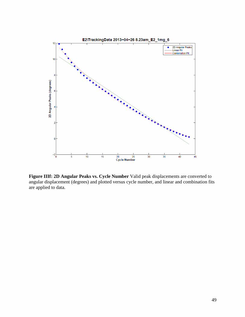
Figure IIIf: 2D Angular Peaks vs. Cycle Number Valid peak displacements are converted to

angular displacement (degrees) and plotted versus cycle number, and linear and combination fits

are applied to data.