Embed Size (px)
Citation preview

Characterizing the Variance Risk Premium in
Consumption-Based Models∗
Guanglian Hu
ITAM
Kris Jacobs
University of Houston
Sang Byung Seo
University of Houston
August 6, 2018
Abstract
We show that in a general consumption-based asset pricing model with Epstein-Zin preferences,
the market variance risk premium is linearly related to the leverage effect, the conditional
covariance between the market return and its variance. This relation is due to the pricing of
volatility risk. Empirically, we document a positive and statistically significant relationship
between the variance risk premium and the leverage effect, using 1990-2016 data for the S&P
500 index. We exploit the relation between the variance risk premium and the leverage effect to
characterize the historical behavior of the market variance risk premium dating back to 1926.
∗We thank Torben Andersen, Don Carmichael, Hitesh Doshi, Bjørn Eraker, Nicola Fusari, Jianfeng Hu, Mete Kilic, PraveenKumar, Yuanshun Li, Kian Guan Lim, Hong Liu, Rui Liu, Felix Matthys, Daniela Osterrieder, Rogier Quaedvlieg, LawrenceSchmidt, Ivan Shaliastovich, Rauli Susmel, Victor Todorov, Jun Tu, Aurelio Vasquez, Vadym Volosovych, Guojun Wu, YangruWu, James Yae, Jun Yu, Joe Zhang, Guofu Zhou, and seminar participants at the University of Houston, ITAM, RyersonUniversity, Rutgers University, Erasmus, Singapore Management University, the MFA meetings and the SoFiE Summer Schoolat Northwestern University for helpful discussions and comments. All remaining errors and omissions are ours.

1 Introduction
The variance of returns is one of the building blocks of modern finance, and fortunately it is
possible to characterize and measure it very precisely, even over very short intervals. We now
also have estimates of the variance risk premium, the difference between physical and risk-
neutral expectations of future market return variance, following the growth in derivatives
markets over the past few decades. The measurement and characterization of the variance
risk premium has generated a lot of attention from academics as well as practitioners because
it reveals how variance risk is perceived and incorporated into prices by investors. The
existing literature finds that the variance risk premium is large, negative, and statistically
significant. It is a strong predictor of short-horizon future market returns.1 Several models
featuring time-varying economic uncertainty have been proposed to explain these stylized
facts in the data.
This paper shows that in a general consumption-based asset pricing framework, the
variance risk premium is linearly related to leverage effect, which we define as the conditional
covariance between the market return and its variance. While there is an extensive literature
on the leverage effect starting with Black (1976), this relation to the variance risk premium
has not yet been documented.
The relation between the variance risk premium and the leverage effect is driven by the
pricing of volatility risk. If volatility risk is priced, shocks to the market variance result in
shocks to the pricing kernel, and therefore in shocks to the market return. The variance
risk premium measures how the market variance co-moves with the pricing kernel, while the
leverage effect measures how the market variance co-moves with the market return. In other
words, the variance risk premium and the leverage effect are generated through the same
channel.
1Bollerslev, Tauchen, and Zhou (2009) document that the variance risk premium is a strong predictor ofshort-term U.S. equity market returns. Bollerslev, Marrone, Xu, and Zhou (2014) provide additional evidencebased on international data. Kilic and Shaliastovich (2018) decompose the total variance risk premium intogood and bad components and investigate the predictive power of each component.
1

We empirically confirm the theoretical relation between the variance risk premium and
the leverage effect using monthly data on the S&P 500 for 1990-2016. We document a
strong and statistically significant positive linear relationship between the two quantities,
consistent with the theory. This finding is robust to alternative measurement of the variance
risk premium and the leverage effect and obtains for various sample periods. These findings
suggest that investors are willing to pay a higher premium for hedging against volatility risk
when they expect stronger (i.e. more negative) co-movement between returns and volatility.
The relation between the variance risk premium and the leverage effect can be used
to empirically study and document the properties of the variance risk premium. As an
example, we provide estimates of the variance risk premium dating back to 1926, which is
possible because the leverage effect can be estimated provided that daily market returns are
available. Existing estimates of the variance risk premium typically start in 1990 because
sufficient index option data are not available prior to this time. The resulting time series of
the variance risk premium are therefore far more limited compared to available return time
series as well as most other financial and economic variables. We find that the extended time
series of the variance risk premium we construct has plausible properties. The variance risk
premium is very large and displays extreme fluctuations during the late 1920s and throughout
the 1930s, reflecting the adverse economic conditions during the Great Depression.
Our paper contributes to the expanding empirical literature on the variance risk premium.
While a long position in the market index itself results in a positive expected return, it is well
known that a long position in the second moment of the index on average generates significant
losses. For instance, Coval and Shumway (2001) and Bakshi and Kapadia (2003) show that
option-based strategies that are long index variance, such as delta-hedged portfolios and
zero-beta straddles, earn negative average returns.2 Recent evidence from volatility claims
(e.g. variance swaps and VIX futures), which are designed to offer investors direct exposure
to volatility risk, also documents a large negative variance risk premium (Carr and Wu, 2009;
2Another strand of literature investigates the pricing of volatility risk in the cross-section of stock returns.See, for example, Ang, Hodrick, Xing, and Zhang (2006).
2

Aı̈t-Sahalia, Karaman, and Mancini, 2015; Eraker and Wu, 2017). Related, Todorov (2010)
investigates the time series dynamics of the variance risk premium.
Several existing studies examine the variance risk premium in the context of consumption-
based models with Epstein-Zin preferences. To explain the variance risk premium, the con-
sumption dynamics originally proposed in the long-run risk model of Bansal and Yaron
(2004) have been extended in several ways. For example, Bollerslev, Tauchen, and Zhou
(2009) incorporate stochastic volatility-of-volatility into consumption growth, and Zhou and
Zhu (2014) consider long-run and short-run components of consumption growth. Drechsler
and Yaron (2011) augment the long-run risk model by introducing jumps into the model,
emphasizing their importance in explaining the variance risk premium.3 Separately, Seo
and Wachter (2018) show that a model with stochastic disaster risk can also account for the
variance risk premium. While these papers relate the variance risk premium to the dynamics
of economic fundamentals like consumption growth, we focus on the relation between the
variance risk premium and the leverage effect within a general theoretical setup.4
We also contribute to the literature on the leverage effect and asymmetric volatility.5
Existing studies show that the leverage effect for the index is robustly negative. The negative
sign implies that volatility responds asymmetrically to positive and negative returns. Black
(1976) attributes this phenomenon to firm leverage, which is the origin of the terminology
“leverage effect.” When the stock price is lower, financial/operating leverage goes up, which
makes the stock riskier and more volatile.6 Bekaert and Wu (2000) empirically reject the
leverage channel and instead support an alternative hypothesis based on time-varying risk
premia, the volatility feedback effect. If volatility is negatively priced, a positive shock to
3Eraker (2008) also considers a similar model where the consumption variance process is subject to aPoisson jump.
4Our benchmark model in Section 2 is the continuous-time version of the long-run risk model of Bansaland Yaron (2004). This setup is extended in Section 6, which makes it possible to nest a wider range ofmodels including the generalized long-run risk model (Drechsler and Yaron, 2011) and rare disaster models(Barro, 2006; Wachter, 2013).
5Alternatively, in the existing literature the leverage effect may refer to the the correlation between returnand variance.
6This leverage hypothesis is also studied by Christie (1982), Schwert (1989), and Cheung and Ng (1992).
3

volatility leads to an immediate increase in investors’ marginal utility and a decrease in the
stock price, producing asymmetric volatility.7 Note that we do not necessarily take a stance
on which channel is more empirically plausible, but the model we use in this paper, like
most other dynamic consumption-based models, generates the leverage effect through the
volatility feedback channel.
The rest of the paper is organized as follows. Section 2 derives a theoretical relation
between the variance risk premium and the leverage effect using the benchmark model.
Section 3 discusses various aspects of this relation. Section 4 presents the main empirical
analyses. Section 5 provides robustness results. Section 6 discusses a more general model.
Section 7 concludes.
2 The Model
In this section, we present our main result. We deliberately focus on a simple version of the
model to provide intuition for this result. In Section 6, we show that this result also obtains
in a model with jumps and/or rare events, which is more general and is capable of matching
additional stylized facts in equity index markets.
2.1 Model Setup
We assume that aggregate consumption Ct follows an affine diffusion process
dCtCt−
= (µC +Xt)dt+√VtdBC,t,
where BC,t is a standard Brownian motion. The drift of consumption growth has a time-
varying component, Xt, which mean-reverts back to zero. The variance of consumption
7Other studies on the volatility feedback effect include French, Schwert, and Stambaugh (1987) andCampbell and Hentschel (1992). Bandi and Reno (2012) and Yu (2012) report evidence for a time-variationin the leverage effect.
4

growth Vt is stochastic as well and follows the square root process of Cox, Ingersoll, and
Ross (1985). This gives:
dXt = −κXXtdt+ σX√VtdBX,t
dVt = κV (V̄ − Vt)dt+ σV√VtdBV,t, (1)
where BX,t and BV,t are also standard Brownian motions that are independent of each other
and of BC,t.
We assume complete markets with an infinitely-lived representative agent who has recur-
sive preferences as in Epstein and Zin (1989) and Weil (1989). The utility function implied
by Epstein-Zin preferences generalizes time-additive power utility by allowing the separation
of relative risk aversion and the elasticity of intertemporal substitution (EIS). We adopt the
continuous-time formulation of this utility function derived in Duffie and Epstein (1992):
Jt = EP[∫ ∞
t
f(Cs, Js)ds
](2)
where
f (C, J) =δ
1− 1ψ
(1− γ)J
[(C [(1− γ) J ]−
11−γ
)1− 1ψ − 1
]. (3)
The parameters δ, γ, and ψ represent the rate of time preference, relative risk aversion, and
the EIS, respectively. While the expression for the normalized aggregator f is defined only
when the EIS is not equal to one, the limit of the EIS approaching one is well-defined.8
In this paper, we are agnostic about different choices of model parameters as our focus
is to make a general statement about the relationship between the variance risk premium
8That is, in case of a unit EIS, the normalized aggregator is defined as
limψ→1
f(C, J) = δ(1− γ)J
[logC − 1
1− γlog [(1− γ) J ]
].
5
and the leverage effect. However, it is still worth mentioning that our setup reduces to (the
continuous-time analogue of) the long-run risk model of Bansal and Yaron (2004) given a
calibration in which the mean and volatility components of consumption growth are highly
persistent and the representative agent prefers early resolution of uncertainty (ψ > 1γ> 1).
In Section 6, we extend the current setup to incorporate the risk of jumps, in an effort to
also nest other models (e.g. Drechsler and Yaron, 2011; Wachter, 2013) in our setup.
The value function J is a function of the three state variables (Ct, Xt, and Vt). Since the
functional form of the normalized aggregator implies that the value function is homogeneous
of degree (1− γ) in consumption, it follows that
Jt =C1−γt
1− γI(Xt, Vt), (4)
where I(·) needs to be determined. In general, dynamic Epstein-Zin models do not allow
an exact closed-form solution for I unless the EIS equals one. Appendix A shows that we
obtain an exponentially linear function
I(X, V ) = ea+bXX+bV V (5)
for an arbitrary EIS, where a, bX and bV are defined in the Appendix. This result uses
an approximation around the mean consumption-wealth ratio proposed by Campbell and
Viceira (1999). In case of a unit EIS, this approximation is exact.
Based on equation (4) and the results from Duffie and Skiadas (1994), Appendix B derives
the stochastic differential equation for the state-price density πt as
dπtπt−
= −rf,tdt− γ√VtdBC,t +
(1− 1
θ
)[bXσX
√VtdBX,t + bV σV
√VtdBV,t
], (6)
where θ = (1 − γ)/(1 − 1/ψ) and rf,t is the instantaneous risk-free rate. For details, see
Appendix B.
6

2.2 Stock Price Dynamics
We define the aggregate stock as the claim to the aggregate dividend Dt, which evolves
according to
dDt
Dt−= µD,tdt+ φ
√VtdBC,t,
where µD,t = µD0 + µDXXt + µDV Vt.9
The pricing relation implies that the price of this dividend claim, St, equals the ex-
pected future cash flows discounted by the state-price density. In Appendix C, we derive the
following expression for St:
St = EPt[∫ ∞
t
πsπtDsds
]= Dt
∫ ∞0
exp(aφ(τ) + bφX(τ)Xt + bφV (τ)Vt
)dτ,
where aφ(τ), bφX(τ), and bφV (τ) solve a system of ordinary differential equations provided
in the Appendix. Note that the price-dividend ratio, G(Xt, Vt) = St/Dt, is not exactly a
log-linear function of Xt and Vt, although it is fairly close because it is an integral of a
log-linear function. Following Seo and Wachter (2017), we log-linearize the price-dividend
ratio as:10
G(X, V ) ' exp(aφ̄ + bφ̄XX + bφ̄V V
), (7)
where aφ̄, bφ̄X , and bφ̄V are defined in the Appendix. By applying Ito’s lemma to St = DtGt,
the dynamics of the stock price are given by
dStSt−
= µS,tdt+ φ√VtdBC,t + bφ̄XσX
√VtdBX,t + bφ̄V σV
√VtdBV,t. (8)
9This general specification of the dividend process nests the standard assumption that the aggregatedividend is a levered consumption claim (i.e. Dt = Cφt ), in which case µD,t = φµC + φXt + 1
2φ(φ − 1)Vt.Since dividends are more volatile than consumption, in this specification φ is assumed to be larger than 1.
10It is convenient to log-linearize this function; without this, the dynamics of the stock price do not exactlyfollow an affine-jump diffusion process.
7

For additional details, see Appendix C.
We also derive the risk-neutral dynamics of the stock price in the model. Based on the
Radon-Nikodym derivative process Lt = πt
(∫ t0rf,sds
)implied by equation (6), Girsanov’s
theorem suggests
dStSt−
= µQS,tdt+ φ√VtdB
QC,t + bφ̄XσX
√VtdB
QX,t + bφ̄V σV
√VtdB
QV,t, (9)
where BQC,t, B
QX,t, and BQ
V,t are standard Brownian motions under the risk-neutral measure
defined in Appendix B. Under the risk-neutral measure, the drift of the stock dynamics
becomes the risk-free rate less the dividend yield (i.e. µQS,t = rf,t −G−1t ).
2.3 The Variance Risk Premium
The variance risk premium is defined as the difference between the physical and risk-neutral
expectations of future realized variance.11 Empirically, realized variance is measured as the
sum of squared high-frequency log returns over an interval. This quantity converges to the
quadratic variation of the log stock price as the sampling interval becomes smaller. Thus,
in the model, we calculate realized variance using the quadratic variation
QVt,t+τ =
∫ t+τ
t
d [logS, logS]s =
∫ t+τ
t
ξVsds, (10)
where ξ =(φ2 + b2
φ̄Xσ2X + b2
φ̄Vσ2V
). We define V S
t ≡ ξVt as the time-t instantaneous stock
variance. The use of quadratic variance makes it easy to analytically calculate expectations
of realized variance and the variance risk premium in our model.
11Existing studies report a sizable variance risk premium at the index level (e.g., Bakshi and Kapadia, 2003;Carr and Wu, 2009). Additional evidence for the existence of the index variance risk premium is providedin the option pricing literature (e.g., Bates, 2000; Pan, 2002; Eraker, 2004). The variance risk premium isa strong predictor of short term stock index returns (Bollerslev, Tauchen, and Zhou, 2009). Zhou (2018)provides a comprehensive survey on the predictive power of the variance risk premium.
8

The time-t variance risk premium between t and t+ τ is given by:
V RPt,t+τ = EPt [QVt,t+τ ]− EQt [QVt,t+τ ] = ξ
(EPt[Vt,t+τ
]− EQt
[Vt,t+τ
]), (11)
where Vt,t+τ =(∫ t+τ
tVsds
)is the integrated consumption variance between t and t+τ . EP [·]
and EQ[·] represent expectations under the physical and risk-neutral measure, respectively.
We calculate the closed-form expression for equation (11) in Appendix D. Under both
measures, the time-t conditional expectation of Vt,t+τ is linear in Vt with coefficients that
are functions of τ . Consequently, the time-t variance risk premium in the model is also
obtained as a linear function of Vt.
Equation (11) indicates that the model-implied variance risk premium arises from the
stochastic volatility in equations (8) and (9). In a dynamic Epstein-Zin model, shocks to
Vt (i.e. dBV,t) are priced, which makes the risk-neutral dynamics of Vt different from its
physical counterpart. Specifically, under the risk neutral measure,
dVt = κQV (V̄ Q − Vt)dt+ σV√VtdB
QV,t
where κQV = κV −(1− 1
θ
)bV σ
2V and V̄ Q = V̄ κV /κ
QV . See Appendix B for details. Since
Vt and, by extension, Vt,t+τ have different conditional means under the two measures, the
model-implied variance risk premium is nonzero.12
12The literature has documented the important role of jump risk in explaining the variance risk premiumin the data. Drechsler and Yaron (2011) find that the long-run risk model enhanced by jumps is able toexplain the behavior of the variance risk premium. The results in Todorov (2010), Bollerslev and Todorov(2011), and Bollerslev, Todorov, and Xu (2015) also suggest that the compensation for jump risk accountsfor a large fraction of the variance risk premium. To illustrate that our findings can accommodate thesestylized facts, Section 6 presents an extension of the model where the variance risk premium is also drivenby jump risk.
9
2.4 The Leverage Effect and the Variance Risk Premium
In many empirical applications, the variance risk premium is measured over a one-month
time horizon τ . For such short horizons, the integrated variance Vt,t+τ =(∫ t+τ
tVsds
)is well
approximated by τVt+τ . Thus, in this case, it follows that
V RPt,t+τ ' ξ
(EPt [τVt+τ ]− EQt [τVt+τ ]
)= EPt
[τV S
t+τ
]− EQt
[τV S
t+τ
], (12)
where τV St+τ represents the stock variance over horizon τ . This approximation provides
intuition by simplifying the expression for the variance risk premium, eliminating integrals
over short horizons. However, Appendix D and Appendix E indicate that this approximation
is not required to derive our main result, the linear relationship between the variance risk
premium and the leverage effect. Note also that if the continuous-time model is implemented
in discrete time using one-month intervals, this approximation is exact.
Since the Radon-Nikodym derivative Lt is a martingale, we know that EPt [Lt+1/Lt] = 1.
Furthermore, it follows from the Radon-Nikodym theorem that EQt [V St+τ ] = EPt
[Lt+τLtV St+τ
].
These two relations imply that equation (12) can be expressed as
V RPt,t+τ =
(EPt[Lt+τLt
]EPt[τV S
t+τ
]− EPt
[Lt+τLt
τV St+τ
])= −Covt
(Lt+τLt
, τV St+τ
). (13)
The expression for (Lt+τ − Lt)/Lt is given by:
Lt+τ − LtLt
= −γ√Vt∆BC +
(1− 1
θ
)[bXσX
√Vt∆BX + bV σV
√Vt∆BV
]. (14)
where ∆BC , ∆BX , and ∆BV are Brownian increments that are normally distributed with
mean 0 and variance τ . It can be seen from equation (6) that this is the innovation to the
pricing kernel.13 Equation (13) therefore states that the time-t variance risk premium is the
time-t covariance between the innovation to the stock variance (τV St+τ −EPt
[τV S
t+τ
]) and the
13This result also follows from the fact that Lt is a martingale with dLt/Lt− = dπt/πt− + rf,tdt.
10

innovation to the pricing kernel.
This expression is analogous to the economic intuition behind the equity premium: the
equity premium originates from the covariance between the innovations to the stock re-
turn and the pricing kernel. Equation (13) addresses the second moment, while the equity
premium addresses the first moment.
The pricing kernel contains several shocks, but only ∆BV is relevant to the variance
premium. While the ∆BC and ∆BX shocks are uncorrelated with the innovation to the
stock variance, ∆BV is, by definition, the shock to the consumption variance Vt and is
perfectly correlated with the shock to the stock variance V St . Since the loading on this shock
in equation (14) is(1− 1
θ
)bV σV
√Vt, equation (13) becomes
V RPt,t+τ = −(
1− 1
θ
)bVbφ̄V
Covt
(bφ̄V σV
√Vt∆BV , τV
St+τ
). (15)
As can be seen from equation (8), the term bφ̄V σV√Vt∆BV is the only part of the log stock
price dynamics that is correlated with the shock to the stock variance. Thus, equation (15)
can also be expressed as
V RPt,t+τ = −(
1− 1
θ
)bVbφ̄V
Covt(logSt+τ , τV
St+τ
), (16)
where Covt(logSt+τ , τV
St+τ
)= Covt
(log St+τ
St, τV S
t+τ
)is the conditional covariance between
the log stock return and stock variance, which we refer to as the leverage effect in the stock
market. We denote this quantity as LEt,t+τ . Equation (16) shows that the variance risk
premium is affine, i.e. linear with zero intercept, in the leverage effect.
Recall that this derivation assumes a short horizon τ and the absence of jumps. Section 6
and Appendix D show that even in a setup with jumps, we obtain a similar result for arbitrary
τ ; however, in this case the variance risk premium is linear in the leverage effect with a
11
nonzero intercept
V RPt,t+τ = α + βLEt,t+τ . (17)
Equation (17) is the main relation analyzed in our empirical work.
3 Discussion
The model generates a nontrivial variance risk premium because shocks to volatility are
priced. In Section 3.1, we emphasize the critical role of Epstein-Zin preferences, which allow
for volatility risk to be priced in the model. In the resulting economy, there is an economically
intuitive relation between the leverage effect and the variance risk premium due to the pricing
of volatility risk. We explain the intuition behind this relation in Section 3.2. In Section 3.3,
we discuss the relation between the variance risk premium, the leverage effect, and the
variance of variance.
3.1 The Role of Recursive Preferences
The model economy uses the continuous-time formulation of Epstein-Zin recursive utility in
Duffie and Epstein (1992). We adopt a continuous-time framework for analytical convenience.
However, the use of non-time-separable recursive utility is critical because it generalizes time-
additive power utility and allows for preferences over the timing of uncertainty resolution.
The agent prefers early (late) resolution of uncertainty when ψ is greater (smaller) than 1/γ.
To appreciate the importance of this model feature, consider the case of power utility,
which means that the timing of uncertainty resolution is irrelevant. This special case can be
obtained by setting ψ = 1γ. The state-price density in equation (6) then becomes
dπtπt−
= −rf,tdt− γ√VtdBC,t. (18)
12

That is, shocks to the mean and the variance of consumption growth (i.e. dBX,t and dBV,t)
disappear because(1− 1
θ
)equals zero.14
Comparing equation (18) with equation (6) highlights the implications of the utility
function for the variance risk premium. Shocks to the variance no longer enter the state-
price density, and therefore also do not enter the pricing kernel in equation (14). In other
words, the innovation to the pricing kernel is no longer correlated with the innovation to the
variance, and the variance risk premium is zero.
Alternatively, this implication can be directly verified from the expression for the variance
risk premium in equation (15): the right-hand side of equation (15) simply becomes zero
under power utility because the coefficient(1− 1
θ
)is zero.
3.2 Why is the Relation Linear?
The definitions of the variance risk premium and the leverage effect provided in Section 2.4
provide intuition for why these two quantities are so closely connected. We have:
V RPt,t+τ = −Covt(τV S
t+τ ,Mt+τ
)(19)
LEt,t+τ = Covt(τV S
t+τ , rS,t+τ), (20)
where Mt+τ ≡ Lt+τLt
is the pricing kernel and rS,t+τ ≡ log St+τSt
is the log return on the
aggregate market.
Equation (19) states that the variance risk premium is (the negative of) the covariance
between the stock variance and the pricing kernel. In the model, the stock variance is a
constant multiple of the consumption variance: V St+τ = ξVt+τ . Thus, the innovation to the
stock variance originates from the innovation to the consumption variance (i.e. σV√Vt∆BV ).
By assuming Epstein-Zin preferences, such shocks are priced and thus appear in the pricing
kernel with a loading of(1− 1
θ
)bV as shown in equation (6). Typically, this loading is
14Since γ is equal to the inverse of ψ, the parameter θ = (1− γ)/(1− 1/ψ) is one under power utility.
13
assumed to be positive so that the marginal utility of the representative agent rises when
there is a positive volatility shock. This positive co-movement between the stock variance
and the pricing kernel generates a negative variance risk premium.
Furthermore, the pricing of volatility risk generates the so-called volatility feedback ef-
fect, as documented, for example, by French, Schwert, and Stambaugh (1987), Campbell
and Hentschel (1992), and Bekaert and Wu (2000). A positive shock to the pricing kernel
originated from a positive volatility shock would lead to a higher required return on the ag-
gregate market, which in turn causes a drop in the stock price. The stock variance therefore
exhibits a negative co-movement with the stock return through this volatility feedback chan-
nel. In the model, equation (8) clarifies this relation. The loading of the stock return on the
innovation to the variance is bφ̄V , and this coefficient is typically calibrated to be negative
(so the price-dividend ratio is low when Vt is high). This negative coefficient generates a
negative leverage effect according to equation (20).
We conclude that the variance risk premium and the leverage effect arise from the same
source: the pricing of volatility risk. The two quantities measure how the stock variance
comoves with others; the former is with the pricing kernel while the latter is with the stock
return. Since the pricing kernel and the stock return are both affected by shocks to variance
under an economy where volatility risk is priced, it naturally follows that the variance risk
premium and the leverage effect are closely associated.
In our model, these two quantities are linearly related. Note that the loadings of the
pricing kernel and the stock return on the innovation to variance are(1− 1
θ
)bV and bφ̄V ,
respectively. Thus, the linear coefficient between the variance risk premium and the leverage
effect becomes (the negative of) the ratio of these two loadings, namely[−(1− 1
θ
)bVbφ̄V
], as
can be seen from equation (16).
It is worth noting the role of the log-linear approximation in demonstrating this linear
relation. Under Epstein-Zin utility, a dynamic model does not permit an exact closed-form
solution unless the EIS is one. Hence, in Section 2, we follow Campbell and Viceira (1999)
14
and approximate the value function in closed form.15 However, this does not imply that
the relation between the variance risk premium and the leverage effect is an artifact of our
model specification and solution method. The intuition from expressions (19) and (20) is
not model-specific. The pricing of volatility risk ensures that when a volatility shock arrives,
the pricing kernel in equation (19) and the aggregate market return in equation (20) comove
in different directions. In the model, the relation between the variance risk premium and
the leverage effect is linear under the log-linearization, which means that the leverage effect
fully characterizes the variance risk premium. More generally, this relation may not be linear
but could instead include some higher-order effects. For example, Kraus and Litzenberger
(1976) and Dittmar (2002) examine nonlinear pricing kernels that depend on second- and
third-degree polynomials of the market return.16 In these more general setups, the linear
relationship between the variance risk premium and the leverage effect continues to capture
the first-order effect of the volatility feedback channel. We conclude that in general there is
a strong relation between the variance risk premium and the leverage effect.
3.3 The Variance Risk Premium and the Variance of Variance
Economic intuition suggests that variance-of-variance risk is a major determinant of the
variation in the variance risk premium, because the variance risk premium measures the
compensation for the risk associated with changes in variance.17 Is this intuition consistent
with our findings regarding the variance risk premium and the leverage effect?
In Section 2, the consumption variance Vt follows a square root process. This assumption
is made for parsimony because it ensures that the instantaneous variance of consumption
variance, denoted as Wt, is completely determined by the consumption variance Vt itself.
15When the model is written in discrete-time, the log-linear approximation of Campbell and Shiller (1988)is necessary.
16Other examples include Barone-Adesi (1985) and Harvey and Siddique (2000).17Another potential determinant of the time variation in the variance risk premium is time-varying jump
risk (see, for example, Todorov, 2010). Section 6 extends the benchmark model in Section 2 by incorporatingjump risk.
15

From equation (1), Wt = σ2V Vt, which implies that variance risk and variance-of-variance
risk are perfectly correlated in the model. To further explore the relation among variance-
of-variance risk, the variance risk premium, and the leverage effect, we therefore use the
extension of the volatility dynamics, following Bollerslev, Tauchen, and Zhou (2009), Boller-
slev, Sizova, and Tauchen (2012), and Tauchen (2012):
dVt = κV (V̄ − Vt)dt+√WtdBV,t
dWt = κW (W̄ −Wt)dt+ σW√WtdBW,t,
where BW,t is an independent standard Brownian motion.
The implications of this model extension for the aggregate stock index are straightfor-
ward. First, the price-dividend ratio becomes a function ofWt as well asXt and Vt. Reflecting
this additional source of aggregate market volatility, the stock price dynamics follow
dStSt−
= µS,tdt+ φ√VtdBC,t + bφ̄XσX
√VtdBX,t + bφ̄V
√WtdBV,t + bφ̄WσW
√WtdBW,t.
The coefficient bφ̄W refers to the loading of the log price-dividend ratio on the variance-
of-variance process. Consequently, the instantaneous stock market variance is expressed as
V St = ξV Vt + ξWWt, where ξV =
(φ2 + b2
φ̄Xσ2X
)and ξW =
(b2φ̄V
+ b2φ̄Wσ2W
). It follows from
the definition of the (annualized) leverage effect that
1
τ[LEt,t+τ ] = Covt
(rS,t+τ , V
St+τ
)= τ
[bφ̄V ξV + bφ̄W ξWσ
2W
]Wt. (21)
Under Epstein-Zin preferences, shocks to the new state variable Wt are also priced. The
pricing of variance-of-variance risk yields an additional term in the expression of the state-
price density:
dπtπt−
= −rf,tdt− γ√VtdBC,t +
(1− 1
θ
)[bXσX
√VtdBX,t + bV
√WtdBV,t + bWσW
√WtdBW,t
],
16

where bW determines the market price of variance-of-variance risk. From equation (13), the
(annualized) variance risk premium is derived as
1
τ[V RPt,t+τ ] = −Covt
(Mt+τ , V
St+τ
)= −τ
(1− 1
θ
)[bV ξV + bW ξWσ
2W
]Wt. (22)
Expressions (21) and (22) highlight the added intuition from the extended model. The
time variation in the variance risk premium and the leverage effect are entirely driven by
variance-of-variance risk (Wt), not variance risk (Vt). Note that in Section 2, variance-of-
variance risk is perfectly correlated with variance risk; by replacing the Wt terms in equations
(21) and (22) with σ2V Vt, we indeed obtain the results for the benchmark model.18
We can also express the variance risk premium and the leverage effect in terms of the
variance of variance over horizon τ , which is empirically more relevant than the instanta-
neous variable Wt. The τ -horizon variance of market variance is given by Vart(V St+τ
)=
τ (ξ2V + ξ2
Wσ2W )Wt, which implies that equations (21) and (22) can be written as
1
τ[LEt,t+τ ] =
[bφ̄V ξV + bφ̄W ξWσ
2W
ξ2V + ξ2
Wσ2W
]Vart
(V St+τ
)1
τ[V RPt,t+τ ] = −
(1− 1
θ
)[bV ξV + bW ξWσ
2W
ξ2V + ξ2
Wσ2W
]Vart
(V St+τ
). (23)
The coefficients bφ̄V and[−(1− 1
θ
)bV]
are typically assumed to be negative, as discussed
in Section 3.2. Similarly, bφ̄W and[−(1− 1
θ
)bW]
are usually calibrated to be negative so
the price-dividend ratio falls and the marginal utility rises when variance-of-variance risk
goes up. Since ξV and ξW are positive, the variance risk premium and the leverage effect are
both negatively associated with the variance of market variance: when we expect a higher
variance of market variance, the variance risk premium and the leverage effect become more
negative.
Equation (23) indicates that the variance risk premium is not only linear in the leverage
18In the benchmark model, ξV corresponds to ξ while ξW , bφ̄W , and bW are all zero.
17

effect, but also in the variance of market variance. This suggests an alternative way to
characterize the variance risk premium based on the variance of market variance. In fact,
the variance risk premium, the leverage effect, and the variance of market variance are all
perfectly correlated with one another in the model. Hence, we can equivalently think of the
variance of market variance as generating the variance risk premium.
However, potential distinctions between the leverage effect and the variance of variance
surface when the variance dynamics are subject to shocks that are uncorrelated with the
pricing kernel. Estimates of the variance may be noisy, and this noise is by definition
uninformative about investors’ marginal utility. Furthermore, models such as Johnson (2004)
and Johnson and Lee (2014) emphasize the role of unpriced uncertainty shocks in explaining
various aspects of market data.19
In such circumstances, the leverage effect may be more informative about the variance risk
premium than the variance of market variance. Recall that both the variance risk premium
and the leverage effect are generated through the pricing of volatility risk. This channel
remains in the presence of unpriced volatility shocks. On the other hand, the variance risk
premium and the variance of market variance may differ if some volatility shocks are not
priced. Variance of variance captures every shock to the variance process regardless of its
implications for the pricing kernel. In summary, the leverage effect may characterize the
variance risk premium in a more robust way because both the quantities reflect the pricing
of volatility shocks.
4 Empirical Results
In this section, we construct time series for the variance risk premium and the leverage effect
for the period January 1990 through December 2016, and investigate the empirical relation
19Meanwhile, Dew-Becker, Giglio, Le, and Rodriguez (2017), Dew-Becker, Giglio, and Kelly (2017), andBerger, Dew-Becker, and Giglio (2018) consistently find from various derivatives data that shocks to realizedvolatility are significantly priced whereas shocks to expected future volatility are not.
18

between the two time series. Both time series are available at the monthly frequency; for
notational convenience, we use the time subscript t+ 1 to denote one month from time t.
The variance risk premium is typically measured over one month. We denote it by
V RPt,t+1 for month t. We also calculate the leverage effect over a one-month period, from t
to t+ 1, LEt,t+1. Since there is no ambiguity with respect to the horizon, we simply denote
these two quantities as V RPt and LEt in this section.
4.1 Measuring the Variance Risk Premium and the Leverage Ef-
fect
To calculate the variance risk premium, we need both the physical and risk-neutral expecta-
tions of the future variance, as indicated in equation (11). For the risk-neutral component,
for each month t we take the closing value of the VIX index squared on the last trading
day of the month.20 The squared VIX, which represents the risk-neutral expectation of
the future variance over the subsequent 30 days, is calculated in a model-free way using
out-of-the-money call and put options.21 Since the VIX index is expressed in annualized
percentage volatility terms, we divide the squared VIX by 12 to express it in conventional
units as squared monthly percentages. Denoting this scaled quantity as V IX2t , the variance
risk premium can be expressed as
V RPt = EPt [RVt,t+1]− V IX2t , (24)
where RVt,t+1 is the realized variance between time t and t+ 1.
As demonstrated in the literature, estimating the realized variance based on high-frequency
20The time series of the VIX is obtained from the Chicago Board Options Exchange (CBOE) website.21The CBOE developed the first-ever volatility index in 1993, which was based on Black-Scholes implied
volatilities from at-the-money S&P 100 index options. In 2003, the CBOE modified the methodology andstarted publishing a new VIX index, calculated in a model-free manner based on prices of S&P 500 indexoptions. In this paper, we use the new VIX. For more details on the model-free approach, see Dupire (1994),Neuberger (1994), Britten-Jones and Neuberger (2000), and Jiang and Tian (2005).
19
data provides accurate ex-post measures.22 We obtain the high-frequency S&P 500 index
time series from TICKDATA. While it is possible to further increase our sampling fre-
quency, we follow the standard approach and sample every five minutes to avoid potential
microstructure effects. Liu, Patton, and Sheppard (2015) argue that it is difficult to outper-
form five-minute realized variance even with more sophisticated sampling techniques.
The calculation of the physical expectation proceeds in two steps. First, we calculate the
realized variance RVt,t+1 by summing up the squared five-minute log returns on the S&P
500 index over the month t + 1.23 We multiply the outcome by 10,000 in order to express
realized variance in monthly percentage squared terms. Panel A of Figure 1 presents the
resulting time series from January 1990 to December 2016.
In the second step, we estimate the time-t ex-ante physical variance in equation (24) by
projecting the realized variance between t and t + 1 onto the predictor variables at time t.
Specifically, following Drechsler and Yaron (2011), we consider the following linear projection:
logRVt,t+1 = δ0 + δ1 logRVt−1,t + δ2 log V IX2t + ε. (25)
We use the logarithm of the variance to ensure that variance forecasts always remain pos-
itive.24 Table 1 shows the results from this regression. While the setup is parsimonious,
its predictive power is similar to that of other variance forecasting models, generating an
adjusted R2 of 68%. We consider robustness with respect to the variance forecasting model
in Section 5.1.
The proxy for the time series of EPt [RVt,t+1], which we refer to as ERVt, is obtained using
22See Andersen, Bollerslev, Diebold, and Ebens (2001), Andersen, Bollerslev, Diebold, and Labys (2003),and Barndorff-Nielsen and Shephard (2002).
23For any two consecutive trading days, we calculate the overnight/weekend return and treat it as anadditional five-minute interval of the latter trading day.
24An additional reason to use logarithms is that the distribution of the variance variables is much closerto a log-normal distribution than a normal distribution.
20

the fitted values of the regression:
ERVt = EPt [RVt,t+1] ' exp
(δ0 + δ1logRVt−1,t + δ2logV IX2
t +1
2σ2ε
). (26)
Panel B of Figure 1 shows the time series of ex-ante physical variance estimates together with
that of the squared VIX. Following equation (24), the variance risk premium is measured as
the difference between these two time series, depicted in Panel C.
Now we turn to the leverage effect. We define COVt,t+1 as the realized covariance between
the return on the S&P 500 index and its conditional variance over the month t+ 1. For each
month, we estimate COVt,t+1 using a sample covariance between daily log returns and daily
changes in the conditional variance.25 We estimate the daily time series of conditional vari-
ances using the EGARCH(1,1) model of Nelson (1991), which incorporates the asymmetric
response of volatility to positive and negative returns. In Section 5.2 below, we investigate
if our empirical results are robust to different computations of the leverage effect.
The leverage effect at time t, which we denote as LEt, is calculated as the time-t physical
expectation of COVt,t+1. We estimate LEt using the following linear projection:
COVt,t+1 = δ0 + δ1RVt−1,t + δ2COVt−1,t + ε. (27)
In contrast to equation (25), we do not take logarithms of the covariances because realized
covariance can take on negative as well as positive values. The leverage effect is computed
as the fitted value of the regression:
LEt = EPt [COVt,t+1] ' δ0 + δ1RVt−1,t + δ2COVt−1,t.
Panel B of Figure 2 shows the resulting time series of the leverage effect. Note again that
25In general, calculating realized covariance using high-frequency data is challenging due to asynchronicity(Epps, 1979; Sheppard, 2006). Furthermore, Aı̈t-Sahalia, Fan, and Li (2013) show that leverage effectestimates based on high-frequency data are biased towards zero.
21

the leverage effect is defined in terms of covariance, not correlation.
Panel A of Table 2 reports summary statistics for the variables used in the empirical
analysis: RV (realized variance), ERV (ex-ante physical variance), V IX2 (squared VIX),
V RP (variance risk premium), COV (realized covariance), and LE (leverage effect). We
also include the monthly returns on the S&P 500 index, which we denote as SP .
The sample mean of RV is 19.64. The sample distribution of RV is far from a normal
distribution: it is highly skewed to the right, which makes the median value (10.89) much
lower than the mean. Furthermore, the distribution is extremely fat-tailed, exhibiting a
sample kurtosis of 95.58. Lastly, RV has an AR(1) coefficient of 0.65, implying that it is a
relatively quickly mean-reverting process.
ERV , the ex-ante physical expectation of future realized variance, can be viewed as
a smoothed version of RV because it is obtained by projecting RV of each month onto
predictor variables. ERV is much more persistent, having a monthly AR(1) coefficient of
0.77, and has a skewness (5.58) and kurtosis (47.22) that are much smaller than those of
RV . While the general magnitude of ERV is similar to RV , the mean is slightly smaller
and the median is slightly larger, because the distribution is less skewed.
The squared VIX, which represents the ex-ante risk-neutral expectation of future realized
variance, is on average higher than its physical counterpart (37.01 vs 18.62). This implies
that the variance risk premium is negative on average (-18.39). In fact, the squared VIX is
always larger than the ex-ante physical variance in our sample, which makes the variance
risk premium consistently negative, as evident from Panel C of Figure 1.
Similarly, COV is consistently negative in the sample: the mean value is -16.94 and it is
always negative as illustrated in Figure 2. This is intuitive given that it is a proxy for the
realized covariance between log returns and conditional return variances. LE, the leverage
effect, is obtained as a smoothed version of COV . As we can see in Figure 2, the peak of LE
in October 2008 is much smaller compared to that of COV . While the standard deviation
of LE is smaller compared to COV , other sample statistics are fairly close. For example,
22

the AR(1) coefficients of both variables are 0.77 and 0.78 respectively.
Panel B of Table 2 reports the correlation coefficients among these variables. Evidently,
RV and ERV as well as COV and LE are highly correlated (0.97 and 0.99 respectively).
ERV and V IX2 are also highly positively correlated (0.95) because they are both ex-ante
expectations of future realized variance under two different measures. The fact that V RP
is negatively correlated with both ERV and V IX2 implies that the variance risk premium
becomes larger in magnitude (i.e. more negative) during “bad times” when the volatility
of the market is high. This is consistent with a positive correlation between V RP and
SP , which implies that the variance risk premium becomes smaller in magnitude (i.e. less
negative) during “good times” when the market returns are high.
Importantly, the variance risk premium is significantly and positively correlated with the
leverage effect: the correlation coefficient is 0.46 and in several subsamples this correlation is
even higher. Motivated by this correlation (and our theoretical framework), we investigate
the linear relationship between these two variables more closely in the next section.
4.2 Testing the Linear Relation Between the VRP and the Lever-
age Effect
Based on the time series of the variance risk premium and leverage effect as discussed in
Section 4.1, we empirically examine the theoretical relation derived in equation (17). Specif-
ically, we run the following regression:
V RPt = α + βLEt + εt. (28)
Table 3 displays the outcomes of this regression for various sample periods. As illus-
trated in the first panel, the variance risk premium and the leverage effect are statistically
significantly positively related in the January 1990 through December 2016 sample. The esti-
23

mated slope coefficient β is 0.15 with a Newey-West (1987) t-statistic of 3.27.26 The leverage
effect explains a sizable portion of the variation in the variance risk premium, generating
an adjusted R2 of 21%. The positive relationship implies that times when the variance risk
premium is high (so-called “bad times”) tend to coincide with periods with a high covariance
between the market return and the conditional market variance.
The positive linear relationship between the variance risk premium and leverage effect
is robust to the exclusion of the Great Recession period (December 2007 to June 2009).
The slope coefficient increases (0.43) and is still statistically significant with a Newey-West
t-statistic of 2.65, as can be seen in the second row. The last two rows of Table 3 show the
results from the regression with the two subperiods that are of the same length: the first
half of the sample is from January 1990 to June 2003 and the second half is from July 2003
to December 2016. While both samples yield significantly positive slope coefficients, the
estimates are somewhat different: the estimate for the first period is 0.58, which is larger
than the 0.13 estimate for the second period. The main reason for this difference seems to
be the Great Recession. Table 3 indicates that the estimates for the first half of the sample
and the sample without the Great Recession are similar, presumably because neither sample
contains the Great Recession period. Moreover, the second half of the sample, which includes
the Great Recession period, gives an estimate that is closer to the full sample result. The
leverage effect exhibits an extremely high peak in October 2008, which leads to a smaller
estimate for the slope coefficient. The explanatory power of the leverage effect increases
after splitting the sample into two. Specifically, the values for the adjusted R2 in the first
and second subsamples are 37% and 28% respectively.
The positive relationship between the variance risk premium and the leverage effect is
expected through the lens of an Epstein-Zin asset pricing model. Equation (16) indicates
that the variance risk premium is positively associated with the leverage effect when the
coefficient[−(1− 1
θ
)bVbφV
]is positive. This sign is consistent with economic intuition: a
26The lag selection follows Newey and West (1994).
24

positive(1− 1
θ
)bV means that the marginal utility of the agent rises when Vt is hit by a
positive shock, i.e. during “bad times”, as evident from equation (6). Moreover, bφV is
typically determined to be negative because the price-dividend ratio falls when Vt goes up.
See equation (C.2). Thus, the negative of the ratio between(1− 1
θ
)bV and bφV is expected
to be positive in this model.
4.3 The Variance Risk Premium 1926-2016
The construction of the variance risk premium requires an estimate of the expected future
market variance under the risk-neutral measure. To obtain this risk-neutral expectation, a
large cross section of option prices is required: the squared VIX, which we use as a proxy for
this very quantity for a one-month horizon, is calculated using a range of out-of-the-money
call and put option prices. The available time series of the variance risk premium is therefore
rather limited due to the limited availability of options data. Existing studies of the variance
risk premium focus on a relatively short sample starting in 1990.
Our analysis suggests an alternative approach for constructing a longer time series of the
variance risk premium. Section 2 demonstrates that in a fairly general setup, the variance risk
premium is a linear function of the leverage effect, and this linear relationship is confirmed
in Section 4 using various samples for which both variables are available. Note that the
computation of the leverage effect does not require options data. Our estimate of the leverage
effect can be constructed when daily market returns are available. Thus, we can construct
extended time series of the leverage effect, which in turn can be used to characterize the
variance risk premium over a much longer sample period, based on an estimate of the relation
between the leverage effect and the variance risk premium.
We proceed by estimating the leverage effect starting in January 1926. Daily return data
on the S&P 500 index are available starting in July 1962, but we use the CRSP value-weighted
index as a proxy for the S&P 500 index prior to that. Using this extended time series of
returns, we follow the procedure described in Section 4.1: we run the EGARCH(1,1) model
25

to estimate the daily time series of conditional market variances and calculate the realized
covariance (COV ) for each month as the sample covariance between daily log returns and
daily changes in conditional return variances. We then obtain the leverage effect (LE) by
projecting realized covariance onto lagged realized covariance and realized variance.
We also combine two data sources to estimate the realized variance. High-frequency
index data are available starting in October 1985, and we compute the realized variance
for subsequent months as the summation of the squared five-minute index returns over each
month.27 Prior to October 1985, we compute the realized variance using the French, Schwert,
and Stambaugh (1987) measure, which is the sum of the squared daily log returns over each
month, adjusted for autocorrelations.
Figure 3 shows the extended time series of the variance risk premium, extrapolated based
on the leverage effect. For each month, the variance risk premium V RPt is calculated as
α + βLEt, where α and β are estimated from the sample that excludes the Great Reces-
sion in the second panel of Table 3. We use these estimates rather than those from the
full sample because accurately estimating the variance risk premium and the leverage ef-
fect during the Great Recession is more challenging. Estimates of the slope coefficient are
sensitive to extremely high values of the leverage effect during this period, as discussed in
Section 4.2. Figure 3 indicates that the variance risk premium is consistently negative and
highly time-varying in the long sample. Among occasional downward spikes, a few are no-
ticeable: October 1929 (Black Tuesday or the so-called Great Crash), July 1933 (the depth
of the Great Depression), October 1987 (Black Monday), and October 2008 (the Great Re-
cession). The pattern of the variance risk premium in the 1930s is very distinct: not only is
the level extremely high, it also shows a lot of variation, reflecting the bad economic climate
during the Great Depression. This period is followed by a few decades of economic recovery
after the Second World War where the variance risk premium remains at a low level and
27TICKDATA provides high-frequency index data starting in February 1982, but we found that the dataprior to October 1985 have different trading hours and occasionally contain zero prices. We therefore usethe data starting in October 1985 to avoid biases in the computation.
26
exhibits limited variation. In the extended period, the variance risk premium has a sample
mean of -17.55 and a standard deviation of 8.70.
5 Robustness
We investigate the robustness of the empirical findings in Section 4. We show that the
positive relationship between the variance risk premium and the leverage effect is robust to
alternative measurements of these two variables.
5.1 Alternative Measures of the Variance Risk Premium
Recall that the variance risk premium is defined as the difference between the physical and
risk-neutral expectations of future market variance. While the risk-neutral expectation can
be simply captured by the squared VIX, estimating the corresponding physical counter-
part is generally less straightforward. In our benchmark analysis, we follow Drechsler and
Yaron (2011) and calculate this physical expectation by projecting realized variance onto
lagged realized variance and the squared VIX. In this section, we consider three alternative
projections.
The variance risk premium in Panel A of Figure 4 is constructed under the assumption
that the realized variance process follows a random walk. For each month t, the ex-ante
physical variance is simply EPt [RVt,t+1] = RVt−1,t. This approach, first adopted by Bollerslev,
Tauchen, and Zhou (2009), is popular in the literature partly due to its simplicity. However,
this assumption is somewhat tenuous and it may bias the estimate of the variance risk
premium, especially during highly volatile periods. In fact, Panel A shows that the variance
risk premium has a massive positive spike in October 2008 during the Great Recession. This
is puzzling because we generally expect the variance risk premium to be significantly negative
during bad economic times. Although realized variance was extremely high during October
2008, it is possible that the market did not expect high volatility in the subsequent month.
27

This suggests that at the end of October 2008, the random walk model might overestimate
the expected physical variance, and therefore, the overall variance risk premium.
Panel B of Figure 4 follows Zhou (2018) and calculates the expected physical variance
by assuming that realized variance follows an autoregressive model with 12 lags (AR(12)).
The autoregressive coefficients are estimated based on the full sample period, January 1990
to December 2016.28 Although the time series in Panel B still exhibits some positive spikes
during the Great Recession, their magnitudes are moderate compared to those in Panel A.
Furthermore, in contrast to Panel A, the variance risk premium remains negative most of
the time.
Panel C of Figure 4 considers the variance forecasting model of Bekaert and Hoerova
(2014) using lagged realized variances over different horizons together with the squared VIX
as the predictor variables:
logRVt,t+1 = δ0 + δ1 logRVt−1,t + δ2 logRV Wt + δ3 logRV D
t + δ4 log V IX2t + ε
where RVt−1,t is the monthly realized variance over the month, and RV Dt and RV W
t denote
the realized variances over the last day and last week, respectively. The expectation of the
future realized variance is calculated as
EPt [RVt,t+1] = exp
(δ0 + δ1 logRVt−1,t + δ2 logRV W
t + δ3 logRV Dt + δ4 log V IX2
t +1
2σ2ε
).
The resulting time series of the variance risk premium is consistently negative in the sample
and appears to have a low-frequency pattern that is similar to our benchmark measure.
Panel A of Table 4 examines whether the positive relationship between the variance risk
premium and leverage effect is sensitive to the choice of variance risk premium measures.
Rows (1), (2), and (3) correspond to the models of Bollerslev, Tauchen, and Zhou (2009),
Zhou (2018), and Bekaert and Hoerova (2014), respectively. We report results for the full
28The time series of the resulting variance risk premium can be downloaded from Hao Zhou’s website.
28

sample period as well as for the sample excluding the Great Recession. When using the first
alternative measure with the random walk assumption, the slope coefficient is estimated to
be negative but it is statistically insignificant. The reason is that this variance risk premium
measure exhibits an extremely large positive spike during the Great Recession. When we run
the same regression using the sample without the Great Recession, the estimate of the slope
coefficient is positive. Consistent with our benchmark results, the other two measures based
on Zhou (2018) and Bekaert and Hoerova (2014) always yield significantly positive slope
coefficients regardless of the sample period, demonstrating the robustness of the positive
relationship between the variance risk premium and the leverage effect.
5.2 Alternative Measures of the Leverage Effect
In this section, we construct three alternative measures of the leverage effect. These three
measures as well as our benchmark measure in Section 4.1 differ with respect to the compu-
tation of the realized covariance COV . We use the same projection regression with lagged
realized variance and realized covariance in equation (27) for all four measures. Unlike the
expected physical variance, the leverage effect is relatively less sensitive to different projec-
tion specifications. Recall that our benchmark measure estimates COV using the sample
covariance between daily log returns and daily changes in conditional variances estimated
from the EGARCH(1,1) model.
The computation of COV in the first alternative measure is similar to our benchmark
implementation in that we compute realized covariance between returns and changes in
conditional variance. However, instead of using EGARCH(1,1), here we obtain estimates of
daily conditional variance by applying the variance forecasting model in equation (25) at the
daily frequency. The resulting time series of the leverage effect is displayed in Panel A of
Figure 5.
The second alternative measure simply uses changes in daily realized variances (rather
than changes in the conditional expectations) when computing the sample covariance with
29
daily log returns. For each month, the realized covariance COV is estimated by the sample
covariance between daily log returns and changes in daily realized variances over the month.
Panel B of Figure 5 shows the time series of the leverage effect based on this definition.
Lastly, the third alternative measure considers the sample covariance between daily log
returns and daily variance innovations. For each trading day, we compute the variance
innovation as the realized variance for that day minus the expected one-day ahead realized
variance (i.e. the one-day ahead conditional variance) at the end of the previous trading day.
The leverage effect based on this alternative approach is plotted in Panel C of Figure 5.
Panel B of Table 4 reports the results from regressing the benchmark measure of the
variance risk premium on the three alternative measures of the leverage effect, not only for
the full sample but also for the sample without the Great Recession. Regardless of how
we measure the leverage effect, the estimated slope coefficients are consistently positive and
statistically significant. These results demonstrate that the positive relationship between
the variance risk premium and the leverage effect is robust to various measurements of the
leverage effect.
6 Generalizing the Model
In Section 2, we use a stylized model in order to highlight the mechanics underlying the
relation between the variance risk premium and the leverage effect. However, this model is
not sufficiently rich to explain several important stylized facts of the variance risk premium
(see, for example, Drechsler and Yaron, 2011). We now discuss a more general model that
allows for jump risk in the level of aggregate consumption as well as in its mean and variance.
The model in this section nests the model in Section 2. We demonstrate that this extension
does not change the paper’s main conclusion, the linear relationship between the variance risk
premium and the leverage effect, and that our empirical analysis accounts for the presence
of jumps.
30

We now assume that aggregate consumption follows an affine jump diffusion process
dCtCt−
= (µC +Xt)dt+√VtdBC,t + (eZC,t − 1)dNt,
where Nt is a Poisson process with time-varying intensity λt. The drift and the variance of
consumption growth are also subject to jumps:
dXt = −κXXtdt+ σX√VtdBX,t + ZX,tdNt
dVt = κV (V̄ − Vt)dt+ σV√VtdBV,t + ZV,tdNt.
For notational convenience, we define the vector of jump size distributions as Zt = [ZC,t, ZX,t, ZV,t]>
whose time-invariant distribution is independent of Nt and the Brownian motions.29 This
distribution is characterized by the moment generating function of Zt, which we denote as
ΦZ(u) = EP[eu>Z].
This more general setup includes a wide range of existing consumption-based asset pricing
models that aim to explain the high equity premium and high stock market volatility in the
post-war data. First, the benchmark model in Section 2 is obtained by setting λt ≡ 0. In
this case, with highly persistent mean and volatility components and a representative agent
who prefers early resolution of uncertainty, our setup reduces to the long-run risk model of
Bansal and Yaron (2004). If we allow for jumps in the state variables (except for consumption
growth), we obtain a model that is close to Drechsler and Yaron (2011). Second, note that
different calibrations and parameter values can result in very different models: assuming
large but rare jumps in consumption results in rare disaster models such as Barro (2006)
and Rietz (1988) (who assume constant jump intensity) as well as Wachter (2013) (who
assumes time-varying jump intensity). Our objective is to make a general statement about
the relationship between the variance risk premium and the leverage effect; therefore we do
not impose any restrictions on the model parameters and jump size distributions.
29Since Zt has a time-invariant distribution, we omit the subscript t when it is not necessary.
31

Based on the empirical observation that periods with more frequent jumps usually coin-
cide with higher volatility, it is reasonable to model time-varying jump risk λt as a function
of the stochastic variance Vt. For parsimony, we assume λt = ρ0 + ρV Vt. This simple ap-
proach is fairly standard in the option pricing literature because it has been demonstrated
that separately identifying jump risk and volatility risk can be challenging.30
In Appendix A, we show that the value function Jt has the same functional form as
equation (4). However, the stochastic differential equation for the state-price density πt now
takes an additional jump term:
dπtπt−
=[− rf,t − λt
(ΦZ(ηπ)− 1
)]dt− γ
√VtdBC,t
+
(1− 1
θ
)[bXσX
√VtdBX,t + bV σV
√VtdBV,t
]+(eη>π Zt − 1
)dNt, (29)
where ηπ = [−γ,(1− 1
θ
)bX ,(1− 1
θ
)bV ]>. Appendix B provides the details.
The process for the aggregate dividend Dt is also extended to incorporate jump risk:
dDt
Dt−= µD,tdt+ φ
√VtdBC,t +
(eφZC,t − 1
)dNt.
Based on the new dividend process, Appendix C derives the dynamics for the stock price:
dStSt−
= µS,tdt+ φ√VtdBC,t + bφ̄XσX
√VtdBX,t + bφ̄V σV
√VtdBV,t +
(eη>φ̄Zt − 1
)dNt,
where ηφ̄ = [φ, bφ̄X , bφ̄V ]>. Similarly, the risk-neutral dynamics of the stock price is given by
dStSt−
= µQS,tdt+ φ√VtdB
QC,t + bφ̄XσX
√VtdB
QX,t + bφ̄V σV
√VtdB
QV,t +
(eη>φ̄Zt − 1
)dNt,
where µQS,t = rf,t−G−1t − λ
Qt EQ
[eη>φ̄Zt − 1
]. Under the risk-neutral measure, λt is no longer
30See, for example, Bates (2000), Pan (2002), Eraker, Johannes, and Polson (2003), Eraker (2004), Broadie,Chernov, and Johannes (2007), Christoffersen, Jacobs, and Ornthanalai (2012), and Andersen, Fusari, andTodorov (2015).
32

the intensity process for Nt; instead, we have λQt = λtΦZ(ηπ). The jump intensity remains
linear in Vt under the risk-neutral measure
λQt = ρQ0 + ρQV Vt (30)
with different coefficients ρQ0 = ρ0ΦZ(ηπ) and ρQV = ρV ΦZ(ηπ). Furthermore, the jump
distribution changes as well. The moment generating function of Zt under the risk-neutral
measure is given by
EQ[eu>Z]
= ΦQZ (u) =
ΦZ(u+ ηπ)
ΦZ(ηπ). (31)
In the extended model, the variance risk premium is not only affected by the diffusive
component of the log stock return, but also by the jump component. For notational conve-
nience, let ZS,t = η>φ̄Zt denote the jump size distribution for the log stock price. Since the
quadratic variation is expressed as
QVt,t+τ =
∫ t+τ
t
d [logS, logS]s = ξ
∫ t+τ
t
Vsds+
∫ t+τ
t
Z2S,sdNs, (32)
the variance risk premium consists of two distinctive parts:
V RPt,t+τ = ξ
(EPt[Vt,t+τ
]− EQt
[Vt,t+τ
])+
(EP[Z2S
]EPt[ρ0 + ρVVt,t+τ
]− EQ
[Z2S
]EQt[ρQ0 + ρQVVt,t+τ
]). (33)
Specifically, the second line of equation (33) shows how distinct jump intensities and size
distributions under the two measures affect the variance risk premium. In Appendix D, we
show that the variance risk premium is linear in Vt because the conditional expectation of
Vt,t+τ is linear in Vt regardless of the measure.
The leverage effect is calculated as the time-t conditional covariance between the log
33

stock return and stock variance:
LEt,t+τ = Covt
(log
St+τSt
, τV St+τ
)= EPt
[∫ t+τ
t
d[logS, τV S
]s
].
Appendix E demonstrates that this quantity is linear in Vt as well.
In sum, for any arbitrary τ , both the variance risk premium and the leverage effect
are linear in Vt. This implies that there exist coefficients α and β such that V RPt,t+τ =
α + βLEt,t+τ . In other words, the variance risk premium and the leverage effect exhibit a
linear relationship in the model.
In our theoretical analysis, the relation between the variance risk premium and the lever-
age effect is affine with a zero intercept if the state variables do not exhibit jumps. Table 3
shows that the estimates of the intercept α are between -12 and -16, and are statistically
significant in various sample periods. This finding is consistent with the stylized fact that
jump components are crucial to explaining the dynamics of the variance risk premium.
7 Conclusion
A risk factor pays a premium when it comoves with the pricing kernel. The variance risk
premium captures the conditional covariance between the market variance and the pricing
kernel. A wealth of empirical evidence suggests that the variance risk premium is economi-
cally and statistically significant, which implies that the market variance is correlated with
the pricing kernel and that variance risk is priced.
This paper emphasizes the relation between the variance risk premium and the lever-
age effect in economies with priced volatility risk. We demonstrate this relation in a gen-
eral consumption-based framework that nests various models of the variance risk premium.
Epstein-Zin preferences play a key role in the pricing of volatility risk. When the market
variance is impacted by a shock, this also results in a shock to the pricing kernel and therefore
a shock to the market return. The variance risk premium, which is the covariance between
34

the market variance and the pricing kernel, and the leverage effect, which is the covariance
between the market variance and the market return, therefore result from the same source.
We find that this theoretical relation is supported by the data. Using data for 1990-
2016, we find a strong and positive linear relation between the variance risk premium and
the leverage effect. This result is confirmed in various subsamples and using alternative
measures for the two quantities.
This relation between the variance risk premium and the leverage effect can be used to
empirically study and document the properties of the variance risk premium. As an example,
we provide estimates of the variance risk premium dating back to 1926, which is possible
because the leverage effect can be estimated provided that daily market returns are available.
The relation between the variance risk premium and the leverage effect therefore provides
additional evidence and insight on the variance risk premium, for which currently available
estimates cover a very limited time horizon.
Appendix
This appendix provides detailed derivations for the generalized model in Section 6. The
corresponding results for the benchmark model in Section 2 are obtained as a special case
where jump risk is ignored. This model reduces to the benchmark model by setting ρ0 =
ρV = 0 (i.e. λt ≡ 0) or by setting Zt ≡ 0.
A The Value Function
Adding∫ t
0f(Cs, Js)ds to both sides of equation (2), we obtain
Jt +
∫ t
0
f(Cs, Js)ds = EPt[∫ ∞
0
f(Cs, Js)ds
],
35

where the right-hand side is a martingale by the law of iterated expectations. Hence, the
left-hand side should also be a martingale. Based on the functional form of Jt in equation
(4), it follows from Ito’s lemma that
dJtJt−
+f(Ct, Vt)
Jtdt =
[(1− γ) (µC +Xt)−
IXIκXXt +
IVIκV (V̄ − Vt)−
1
2γ(1− γ)Vt
+1
2
IXXIσ2XVt +
1
2
IV VIσ2V Vt + λtEP
[e(1−γ)ZC,t
ItIt−− 1
]+f(Ct, Vt)
Jt
]dt
+(1− γ)√VtdBC,t +
IXIσX√VtdBX,t +
IVIσV√VtdBV,t
+
(e(1−γ)ZC,t
ItIt−− 1
)dNt − λtEP
[e(1−γ)ZC,t
ItIt−− 1
]dt.
The martingale condition implies that
0 = (1− γ) (µC +Xt)−IXIκXXt +
IVIκV (V̄ − Vt)−
1
2γ(1− γ)Vt
+1
2
IXXIσ2XVt +
1
2
IV VIσ2V Vt + λtEP
[e(1−γ)ZC,t
ItIt−− 1
]+f(Ct, Vt)
Jt, (A.1)
and we can show by combining equations (3) and (4) that
f(Ct, Vt)
Jt=
−δ log I if ψ = 1
δθ(I− 1θ
t − 1)
if ψ 6= 1.
If ψ = 1, it is straightforward that equation (5) satisfies equation (A.1), which implies that
I is an exponentially linear function in X and V . However, when ψ 6= 1, equation (A.1)
does not allow a closed-form solution due to a non-linear term I− 1θ
t . Following Campbell and
Viceira (1999), we log-linearize this term.31 Since δI− 1θ
t represents the consumption-wealth
31See also Campbell and Viceira (2002), Campbell, Chacko, Rodriguez, and Viceira (2004), Nowotny(2011), and Tsai and Wachter (2018).
36

ratio in the model, we can show that
δI−1θ =
C
W= exp
(log
(C
W
))' i0 + i1
(log δ − 1
θlog It
),
where i1 = eEP [log C
W ] and i0 = i1(1− i1). This is essentially the first-order Taylor expansion
of an exponential function around the mean log consumption-wealth ratio. Under this ap-
proximation, it follows that f(Ct,Jt)Jt
' −δθ + θi0 + θi1 log δ − i1 log It, and this implies that
equation (5) becomes a solution for equation (A.1) as in the case with ψ = 1.32 Specifically,
the martingale condition in equation (A.1) becomes
0 =[(1− γ)µC + bV κV V̄ + θ (i0 + i1 log δ − δ)− i1a+ ρ0 (ΦZ(ηJ)− 1)
]+[(1− γ)− bXκX − i1bX
]Xt
+
[−bV κV −
1
2γ(1− γ) +
1
2b2Xσ
2X +
1
2b2V σ
2V − i1bV + ρV (ΦZ(ηJ)− 1)
]Vt, (A.2)
where ηJ = [1 − γ, bX , bV ]>. Since equation (A.2) should hold for arbitrary Xt and Vt, it
follows that
0 = (1− γ)µC + bV κV V̄ + θ (i0 + i1 log δ − δ)− i1a+ ρ0 (ΦZ(ηJ)− 1)
0 = (1− γ)− bXκX − i1bX
0 = −bV κV −1
2γ(1− γ) +
1
2b2Xσ
2X +
1
2b2V σ
2V − i1bV + ρV (ΦZ(ηJ)− 1) .
From this system of equations, we can determine the values of a, bX , and bV .33
32Furthermore, the exact result for ψ = 1 can be obtained as the limit case with ψ → 1 because
limψ→1
f(Ct, Jt)
Jt' limψ→1−δθ + θi0 + θi1 log δ − i1 log It = −δ log It.
33After determining bX from the second equation, the third equation becomes a quadratic equation inbV , which generates two roots. While both roots satisfy the equation, only the negative root remains if weconsider the limit case of the model where σV approaches 0, as discussed in Tauchen (2012).
37
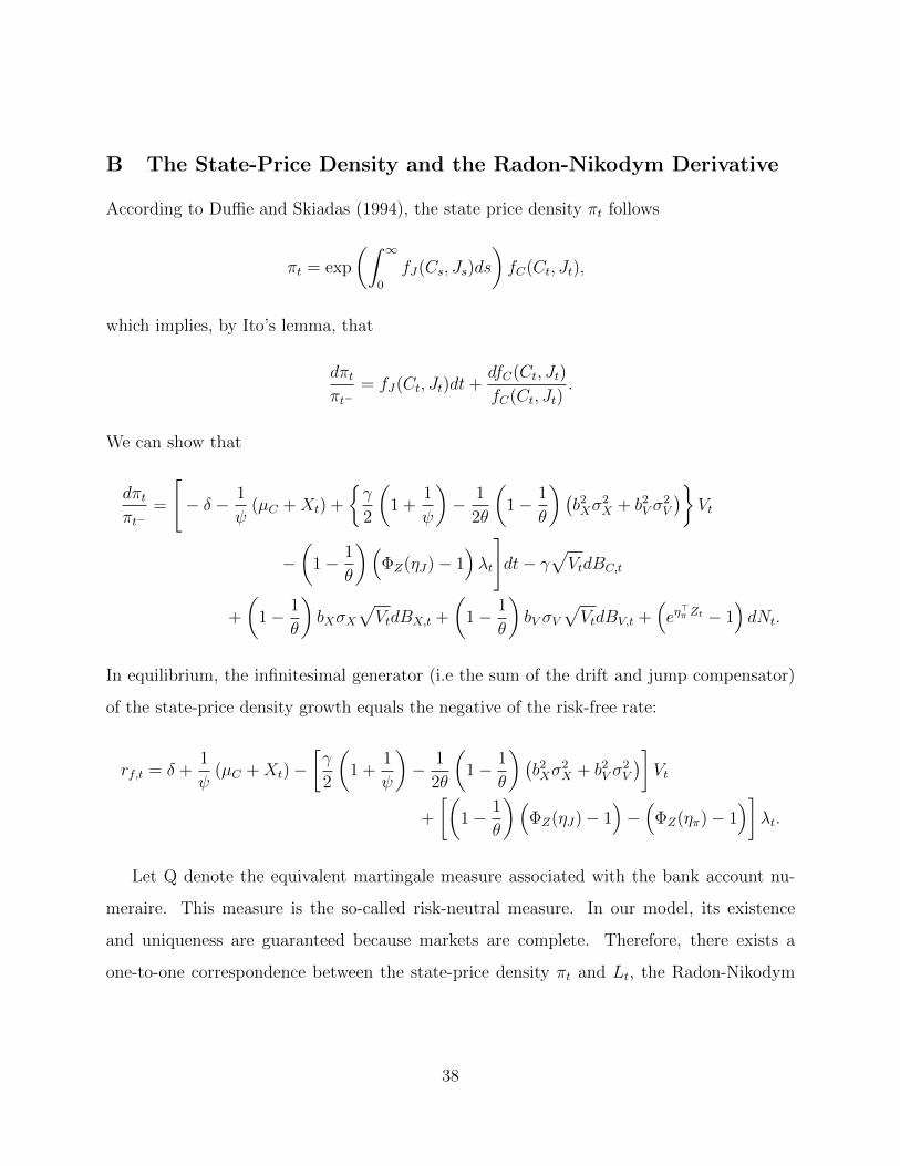
B The State-Price Density and the Radon-Nikodym Derivative
According to Duffie and Skiadas (1994), the state price density πt follows
πt = exp
(∫ ∞0
fJ(Cs, Js)ds
)fC(Ct, Jt),
which implies, by Ito’s lemma, that
dπtπt−
= fJ(Ct, Jt)dt+dfC(Ct, Jt)
fC(Ct, Jt).
We can show that
dπtπt−
=
[− δ − 1
ψ(µC +Xt) +
{γ
2
(1 +
1
ψ
)− 1
2θ
(1− 1
θ
)(b2Xσ
2X + b2
V σ2V
)}Vt
−(
1− 1
θ
)(ΦZ(ηJ)− 1
)λt
]dt− γ
√VtdBC,t
+
(1− 1
θ
)bXσX
√VtdBX,t +
(1− 1
θ
)bV σV
√VtdBV,t +
(eη>π Zt − 1
)dNt.
In equilibrium, the infinitesimal generator (i.e the sum of the drift and jump compensator)
of the state-price density growth equals the negative of the risk-free rate:
rf,t = δ +1
ψ(µC +Xt)−
[γ
2
(1 +
1
ψ
)− 1
2θ
(1− 1
θ
)(b2Xσ
2X + b2
V σ2V
)]Vt
+
[(1− 1
θ
)(ΦZ(ηJ)− 1
)−(
ΦZ(ηπ)− 1)]
λt.
Let Q denote the equivalent martingale measure associated with the bank account nu-
meraire. This measure is the so-called risk-neutral measure. In our model, its existence
and uniqueness are guaranteed because markets are complete. Therefore, there exists a
one-to-one correspondence between the state-price density πt and Lt, the Radon-Nikodym
38

derivative process of Q with respect to the physical measure. It follows that
Lt = πt
(∫ t
0
rf,sds
). (B.1)
Applying Ito’s lemma to equation (B.1) yields
dLtLt−
=dπtπt−
+ rf,tdt,
which subsequently implies
dLtLt−
= −γ√VtdBC,t +
(1− 1
θ
)bXσX
√VtdBX,t +
(1− 1
θ
)bV σV
√VtdBV,t
+(eη>π Zt − 1
)dNt −
(ΦZ(ηπ)− 1
)λtdt︸ ︷︷ ︸
compensated jump
. (B.2)
Equation (B.2) reaffirms that the Radon-Nikodym derivative process is a martingale. Specif-
ically, in our model, Lt consists of four martingales, three of which are Brownian components,
and one of which is a compensated jump.
Girsanov’s theorem dictates how the dynamics of these four martingales change when the
physical measure is switched to the risk-neutral measure. First of all, BC,t, BX,t, and BV,t
are no longer standard Brownian motions under the risk-neutral measures. Instead, BQC,t,
BQX,t, and BQ
V,t are:
BQC,t = BC,t + γ
√Vtdt
BQX,t = BX,t −
(1− 1
θ
)bXσX
√Vtdt
BQV,t = BV,t −
(1− 1
θ
)bV σV
√Vtdt.
Accordingly, we can re-express the dynamics of consumption growth, dividend growth, and
39

the two state variables in terms of Q-Brownian motions:
dCtCt−
= (µC +Xt − γVt) dt+√VtdB
QC,t + (eZC,t − 1)dNt
dDt
Dt−= (µD,t − γφVt)dt+ φ
√VtdB
QC,t +
(eφZC,t − 1
)dNt
dXt =
[−κXXt +
(1− 1
θ
)bXσ
2XVt
]dt+ σX
√VtdB
QX,t + ZX,tdNt
dVt =
[κV −
(1− 1
θ
)bV σ
2V
](κV
κV −(1− 1
θ
)bV σ2
V
V̄ − Vt
)dt+ σV
√VtdB
QV,t + ZV,tdNt.
The change of measure also affects the jump process. Under the risk-neutral measure,
the Poisson process Nt has a different intensity λQt , given by equation (30), and the jump
size distribution Zt follows a different distribution, given by equation (31).34
C The Price-Dividend Ratio
In equilibrium, the stock price (or the price of the dividend claim) is calculated as
St = EPt[∫ ∞
t
πsπtDsds
]=
∫ ∞t
EPt[πsπtDs
]ds.
We define H(Dt, Xt, Vt, s − t) = EPt[πsπtDs
]as the time-t price of the zero-coupon dividend
claim at time s. We conjecture that
Ht = H(Dt, Xt, Vt, τ) = Dt exp(aφ(τ) + bφX(τ)Xt + bφV (τ)Vt
). (C.1)
Using the fact that πtHt = EPt [πsHs] is a martingale (due to the law of iterated expectations),
we verify this conjecture and derive the system of ordinary differential equations that aφ,
34For more details, see Dai and Singleton (2003).
40

bφX , and bφV satisfy. Note that Ito’s lemma implies
d (πtHt)
πt−Ht−=
[− δ − 1
ψµC −
1
ψXt +
{γ
2
(1 +
1
ψ
)− 1
2θ
(1− 1
θ
)(b2Xσ
2X + b2
V σ2V
)}Vt
−(
1− 1
θ
)(ΦZ(ηJ)− 1
)λt + µD,t − bφX(τ)κXXt +
1
2b2φX(τ)σ2
XVt
+ bφV (τ)κV (V̄ − Vt) +1
2b2φV (τ)σ2
V Vt − γφVt +
(1− 1
θ
)bXbφXσ
2XVt
+
(1− 1
θ
)bV bφV σ
2V Vt −
(a′φ(τ) + b′φX(τ)Xt + b′φV (τ)Vt
)]dt
+[φ− γ
]√VtdBC,t +
[bφX(τ) +
(1− 1
θbX
)]σX√VtdBX,t
+
[bφV (τ) +
(1− 1
θ
)bV
]σV√VtdBV,t +
(e[ηπ+ηφ(τ)]
>Zt − 1
)dNt,
where ηφ(τ) = [φ, bφX(τ), bφV (τ)]>. The condition that the infinitesimal generator of this
process equals zero for arbitrary values of Xt and Vt gives us the following system of ordinary-
differential equations
a′φ(τ) = −δ − 1
ψµC + µD0 + bφV (τ)κV V̄
+ρ0
[(ΦZ
(ηπ + ηφ(τ)
)− 1)−(
1− 1
θ
)(ΦZ(ηJ)− 1
)]b′φX(τ) = − 1
ψ+ µDX − bφX(τ)κX
b′φV (τ) = µDV +γ
2
(1 +
1
ψ
)− 1
2θ
(1− 1
θ
)(b2Xσ
2X + b2
V σ2V
)− γφ− bφV (τ)κV
+1
2b2φX(τ)σ2
X +1
2b2φV (τ)σ2
V +
(1− 1
θ
)bXbφXσ
2X +
(1− 1
θ
)bV bφV σ
2V
+ρV
[(ΦZ
(ηπ + ηφ(τ)
)− 1)−(
1− 1
θ
)(ΦZ(ηJ)− 1
)].
41

The boundary conditions for these differential equations are given by
aφ(0) = bφX(0) = bφV (0) = 0,
because H(Dt, Xt, Vt, 0) should be equal to Dt by no-arbitrage.
From this, we can calculate the price-dividend ratio G(Xt, Vt) = St/Dt as follows:
G(Xt, Vt) =
∫ ∞t
exp (aφ(s− t) + bφX(s− t)Xt + bφV (s− t)Vt) ds
=
∫ ∞0
exp (aφ(τ) + bφX(τ)Xt + bφV (τ)Vt) dτ.
As discussed in Section 2.2, G is not a log-linear function of X and V so we use the ap-
proximation in Seo and Wachter (2017). By applying the first-order Taylor approximation
to g(X, V ) = logG(X, V ) around the steady state level (X∗, V ∗), we obtain
g(X, V ) ' g(X∗, V ∗) + gX(X∗, V ∗)(X −X∗) + gV (X∗, V ∗)(V − V ∗).
This equation results in equation (7) when we define
aφ̄ = g(X∗, V ∗)− bφ̄XX∗ − bφ̄V V ∗
bφ̄X = gX(X∗, V ∗) =1
G(X∗, V ∗)
∫ ∞0
bφX(τ) exp (aφ(τ) + bφX(τ)X∗ + bφV (τ)V ∗) dτ
bφ̄V = gV (X∗, V ∗) =1
G(X∗, V ∗)
∫ ∞0
bφV (τ) exp (aφ(τ) + bφX(τ)X∗ + bφV (τ)V ∗) dτ.
This approximation makes it simple to derive the dynamics for the price-dividend ratio:
dGt
Gt
=
[−bφ̄XκXXt + bφ̄V κV (V̄ − Vt) +
1
2bφ̄Xσ
2XVtdt+
1
2bφ̄V σ
2V Vtdt
]dt
+ bφ̄XσX√VtdBX,t + bφ̄V σV
√VtdBV,t +
(ebφ̄XZX,t+bφ̄V ZV,t − 1
)dNt. (C.2)
42

D The Variance Risk Premium
The physical expectation of the quadratic variation in equation (32) equals
EPt [QVt,t+τ ] = ξEPt[∫ t+τ
t
Vsds
]+ EP
[Z2S
]EPt[∫ t+τ
t
λsds
]= ξEPt
[Vt,t+τ
]+ EP
[Z2S
] (ρ0 + ρVEPt
[Vt,t+τ
]).
Therefore, we need to derive the expression for EPt[Vt,t+τ
]. The stochastic differential
equation for Vt implies that
Vu − Vt = κV V̄ (u− t)− κV∫ u
t
Vsds+ σV
∫ u
t
√VsdBV,s +
∫ u
t
ZV,sdNs,
for any u ≥ t. We take time t-expectations on both sides and then differentiate both sides
with respect to u, which results in the following ordinary differential equation:
dEPt [Vu]
du=(ρVEP [ZV ]− κV
)EPt [Vu] + κV V̄ + ρ0EP [ZV ] ,
with the boundary condition EPt [Vt] = Vt. Since this is a first-order linear differential
equation, we can derive its solution as
EPt [Vu] = V̄ ′ + e−κ′V (u−t) (Vt − V̄ ′) ,
where κ′V = κV − ρVEP [ZV ] and V̄ ′ = V̄ + ρ0EP [ZV ] /κ′V . By integrating this solution from
t to t+ τ , we obtain
EPt[Vt,t+τ
]=
∫ t+τ
t
EPt [Vs] ds = τ V̄ ′ +1
κ′V
(1− e−κ′V τ
) (Vt − V̄ ′
). (D.1)
43

Similarly, the risk-neutral expectation of the quadratic variation equals
EQt [QVt,t+τ ] = ξEQt[Vt,t+τ
]+ EQ
[Z2S
]EQt[ρQ0 + ρQVVt,t+τ
], (D.2)
and the conditional risk-neutral expectation of the integrated variance process is calculated
as
EQt[Vt,t+τ
]= τ V̄
′Q +1
κ′QV
(1− e−κ
′QV τ)(
Vt − V̄′Q),
where κ′QV = κQV − ρ
QVEQ [ZV ] and V̄
′Q = V̄ Q + ρQ0 EQ [ZV ] /κ′QV . Given the expressions for
the physical and risk-neutral expectations of quadratic variation, the variance risk premium
is computed as their difference. Since both equations (D.1) and (D.2) are linear in Vt, the
variance risk premium is also linear in Vt.
E The Leverage Effect
We define the time-t leverage effect as the time-t conditional covariance between the log
stock return and stock variance:
LEt,t+τ = Covt
(log
St+τSt
, τV St+τ
)= EPt
[∫ t+τ
t
d[logS, τV S
]s
],
where V St is the time-t instantaneous stock variance. Note that when jumps are present, V S
t
is not simply equal to ξVt, the instantaneous diffusive stock variance. Considering the effect
of jumps, the stock variance can be calculated as V St = limτ→0
1τEPt [QVt,t+τ ]. It follows that
V St = ξ lim
τ→0
1
τEPt[∫ t+τ
t
Vsds
]+ EP
[Z2S
]limτ→0
1
τEPt[∫ t+τ
t
λsds
]= ξVt + EP
[Z2S
]λt.
44

Since this implies that dVS,t =(ξ + ρVEP [Z2
S])dVt, the leverage effect is calculated as
LEt,t+τ = τ(ξ + ρVEP
[Z2S
]){ρ0EP [ZVZS] +
(bφ̄V σ
2V + ρVEP [ZVZS]
)EPt[Vt,t+τ
]},
where the expression for EPt[Vt,t+τ
]is given in equation (D.1).
References
Aı̈t-Sahalia, Yacine, Jianqing Fan, and Yingying Li, 2013, The leverage effect puzzle: Disen-
tangling sources of bias at high frequency, Journal of Financial Economics 109, 224–249.
Aı̈t-Sahalia, Yacine, Mustafa Karaman, and Loriano Mancini, 2015, The term structure of
variance swaps and risk premia, Working paper, Princeton University.
Andersen, Torben G., Tim Bollerslev, Francis X. Diebold, and Heiko Ebens, 2001, The
distribution of realized stock return volatility, Journal of Financial Economics 61, 43–76.
Andersen, Torben G., Tim Bollerslev, Francis X. Diebold, and Paul Labys, 2003, Modeling
and forecasting realized volatility, Econometrica 71, 579–625.
Andersen, Torben G., Nicola Fusari, and Viktor Todorov, 2015, The risk premia embedded
in index options, Journal of Financial Economics 117, 558–584.
Ang, Andrew, Robert J Hodrick, Yuhang Xing, and Xiaoyan Zhang, 2006, The cross-section
of volatility and expected returns, Journal of Finance 61, 259–299.
Bakshi, Gurdip, and Nikunj Kapadia, 2003, Delta-hedged gains and the negative market
volatility risk premium, Review of Financial Studies 16, 527–566.
Bandi, Federico M., and Roberto Reno, 2012, Time-varying leverage effects, Journal of
Econometrics 169, 94–113.
Bansal, Ravi, and Amir Yaron, 2004, Risks for the long-run: A potential resolution of asset
45

pricing puzzles, Journal of Finance 59, 1481–1509.
Barndorff-Nielsen, Ole E., and Neil Shephard, 2002, Econometric analysis of realized volatil-
ity and its use in estimating stochastic volatility models, Journal of the Royal Statistical
Society: Series B (Statistical Methodology) 64, 253–280.
Barone-Adesi, Giovanni, 1985, Arbitrage equilibrium with skewed asset returns, Journal of
Financial and Quantitative Analysis 20, 299–313.
Barro, Robert J., 2006, Rare disasters and asset markets in the twentieth century, Quarterly
Journal of Economics 121, 823–866.
Bates, David S., 2000, Post-’87 crash fears in the S&P 500 futures option market, Journal
of Econometrics 94, 181–238.
Bekaert, Geert, and Marie Hoerova, 2014, The VIX, the variance premium and stock market
volatility, Journal of Econometrics 183, 181–192.
Bekaert, Geert, and Guojun Wu, 2000, Asymmetric volatility and risk in equity markets,
Review of Financial Studies 13, 1–42.
Berger, David, Ian Dew-Becker, and Stefano Giglio, 2018, Uncertainty shocks as second-
moment news shocks, Working paper, Northwestern University.
Black, Fischer, 1976, Studies of stock price volatility changes, Proceedings of the 1976 Meet-
ings of the American Statistical Association, Business and Economic Statistics Section
pp. 177–181.
Bollerslev, Tim, James Marrone, Lai Xu, and Hao Zhou, 2014, Stock return predictabil-
ity and variance risk premia: Statistical inference and international evidence, Journal of
Financial and Quantitative Analysis 49, 633–661.
Bollerslev, Tim, Natalia Sizova, and George Tauchen, 2012, Volatility in equilibrium: Asym-
metries and dynamic dependencies, Review of Finance 16, 31–80.
46

Bollerslev, Tim, George Tauchen, and Hao Zhou, 2009, Expected stock returns and variance
risk premia, Review of Financial Studies 22, 4463–4492.
Bollerslev, Tim, and Viktor Todorov, 2011, Tails, fears, and risk premia, Journal of Finance
66, 2165–2211.
Bollerslev, Tim, Viktor Todorov, and Lai Xu, 2015, Tail risk premia and return predictability,
Journal of Financial Economics 118, 113–134.
Britten-Jones, Mark, and Anthony Neuberger, 2000, Option prices, implied price processes,
and stochastic volatility, Journal of Finance 55, 839–866.
Broadie, Mark, Mikhail Chernov, and Michael Johannes, 2007, Model specification and risk
premia: Evidence from futures options, Journal of Finance 62, 1453–1490.
Campbell, John Y, George Chacko, Jorge Rodriguez, and Luis M Viceira, 2004, Strategic
asset allocation in a continuous-time VAR model, Journal of Economic Dynamics and
Control 28, 2195–2214.
Campbell, John Y., and Ludger Hentschel, 1992, No news is good news: An asymmetric
model of changing volatility in stock returns, Journal of Financial Economics 31, 281–
318.
Campbell, John Y., and Robert J. Shiller, 1988, The dividend-price ratio and expectations
of future dividends and discount factors, Review of Financial Studies 1, 195–228.
Campbell, John Y., and Luis M. Viceira, 1999, Consumption and portfolio decisions when
expected returns are time-varying, Quarterly Journal of Economics 114, 433–495.
Campbell, John Y., and Luis M. Viceira, 2002, Strategic Asset Allocation: Portfolio Choice
for Long-Term Investors. (Oxford University Press).
Carr, Peter, and Liuren Wu, 2009, Variance risk premiums, Review of Financial Studies 22,
1311–1341.
47

Cheung, Yin Wong, and Lilian K. Ng, 1992, Stock price dynamics and firm size: An empirical
investigation, Journal of Finance 47, 1985–1997.
Christie, Andrew A., 1982, The stochastic behavior of common stock variances: Value,
leverage and interest rate effects, Journal of Financial Economics 10, 407–432.
Christoffersen, Peter, Kris Jacobs, and Chayawat Ornthanalai, 2012, Dynamic jump intensi-
ties and risk premiums: Evidence from S&P500 returns and options, Journal of Financial
Economics 106, 447–472.
Coval, Joshua D., and Tyler Shumway, 2001, Expected option returns, Journal of Finance
56, 983–1009.
Cox, John C., Jonathan C. Ingersoll, and Stephen A. Ross, 1985, A theory of the term
structure of interest rates, Econometrica 53, 385–408.
Dai, Qiang, and Kenneth Singleton, 2003, Term structure dynamics in theory and reality,
Review of Financial Studies 16, 631–678.
Dew-Becker, Ian, Stefano Giglio, and Bryan Kelly, 2017, How do investors perceive the
risks from macroeconomic and financial uncertainty? Evidence from 19 option markets,
Working paper, Northwestern University.
Dew-Becker, Ian, Stefano Giglio, Anh Le, and Marius Rodriguez, 2017, The price of variance
risk, Journal of Financial Economics 123, 225–250.
Dittmar, Robert F., 2002, Nonlinear pricing kernels, kurtosis preference, and evidence from
the cross section of equity returns, Journal of Finance 57, 369–403.
Drechsler, Itamar, and Amir Yaron, 2011, What’s vol got to do with it, Review of Financial
Studies 24, 1–45.
Duffie, Darrell, and Larry G Epstein, 1992, Asset pricing with stochastic differential utility,
Review of Financial Studies 5, 411–436.
48

Duffie, Darrell, and Costis Skiadas, 1994, Continuous-time asset pricing: A utility gradient
approach, Journal of Mathematical Economics 23, 107–132.
Dupire, Bruno, 1994, ’Pricing with a smile’, Risk Magazine, Incisive Media pp. 327–343.
Epps, Thomas W., 1979, Comovements in stock prices in the very short run, Journal of the
American Statistical Association 74, 291–298.
Epstein, Larry, and Stan Zin, 1989, Substitution, risk aversion and the temporal behavior of
consumption and asset returns: A theoretical framework, Econometrica 57, 937–969.
Eraker, Bjørn, 2004, Do stock prices and volatility jump? Reconciling evidence from spot
and option prices, Journal of Finance 59, 1367–1404.
Eraker, Bjørn, 2008, The volatility premium, Working paper, University of Wisconsin, Madi-
son.
Eraker, Bjørn, Michael Johannes, and Nicholas Polson, 2003, The impact of jumps in volatil-
ity and returns, Journal of Finance 58, 1269–1300.
Eraker, Bjorn, and Yue Wu, 2017, Explaining the negative returns to VIX futures and ETNs:
An equilibrium approach, Forthcoming, Journal of Financial Economics.
French, Kenneth R., G. William Schwert, and Robert F. Stambaugh, 1987, Expected stock
returns and volatility, Journal of Financial Economics 19, 3–29.
Harvey, Campbell R., and Akhtar Siddique, 2000, Conditional skewness in asset pricing
tests, Journal of Finance 55, 1263–1295.
Jiang, George J., and Yisong S. Tian, 2005, The model-free implied volatility and its infor-
mation content, Review of Financial Studies 18, 1305–1342.
Johnson, Timothy C., 2004, Forecast dispersion and the cross section of expected returns,
Journal of Finance 59, 1957–1978.
49

Johnson, Timothy C., and Jaehoon Lee, 2014, On the systematic volatility of unpriced
earnings, Journal of Financial Economics 114, 84–104.
Kilic, Mete, and Ivan Shaliastovich, 2018, Good and bad variance premia and expected
returns, Forthcoming, Management Science.
Kraus, Alan, and Robert H. Litzenberger, 1976, Skewness preference and the valuation of
risk assets, Journal of Finance 31, 1085–1100.
Liu, Lily Y., Andrew J. Patton, and Kevin Sheppard, 2015, Does anything beat 5-minute RV?
A comparison of realized measures across multiple asset classes, Journal of Econometrics
187, 293–311.
Nelson, Daniel B., 1991, Conditional heteroskedasticity in asset returns: A new approach,
Econometrica 59, 347–370.
Neuberger, Anthony, 1994, The log contract, Journal of Portfolio Management 20, 74–80.
Newey, Whitney K., and Kenneth D. West, 1994, Automatic lag selection in covariance
matrix estimation, Review of Economic Studies 61, 631–653.
Nowotny, Michael, 2011, Disaster begets crisis: The role of contagion in financial markets,
Working paper, Boston University.
Pan, Jun, 2002, The jump-risk premia implicit in options: Evidence from an integrated
time-series study, Journal of Financial Economics 63, 3–50.
Rietz, Thomas A., 1988, The equity risk premium: A solution, Journal of Monetary Eco-
nomics 22, 117–131.
Schwert, William G., 1989, Why does stock market volatility change over time?, Journal of
Finance 44, 1115–1153.
Seo, Sang Byung, and Jessica A. Wachter, 2017, Do rare events explain CDX tranche
50

spreads?, Forthcoming, Journal of Finance.
Seo, Sang Byung, and Jessica A. Wachter, 2018, Option prices in a model with stochastic
disaster risk, Forthcoming, Management Science.
Sheppard, Kevin, 2006, Realized covariance and scrambling, Working paper, University of
Oxford.
Tauchen, George, 2012, Stochastic volatility in general equilibrium, Quarterly Journal of
Finance 1, 707–731.
Todorov, Viktor, 2010, Variance risk-premium dynamics: The role of jumps, Review of
Financial Studies 23, 345–383.
Tsai, Jerry, and Jessica A. Wachter, 2018, Pricing long-lived securities in dynamic endow-
ment economies, Working paper, University of Oxford.
Wachter, Jessica A., 2013, Can time-varying risk of rare disasters explain aggregate stock
market volatility?, Journal of Finance 68, 987–1035.
Weil, Philippe, 1989, The equity premium puzzle and the risk-free rate puzzle, Journal of
Monetary Economics 24, 402–421.
Yu, Jun, 2012, A semiparametric stochastic volatility model, Journal of Econometrics 167,
473–482.
Zhou, Guofu, and Yingzi Zhu, 2014, Macroeconomic volatilities and long-run risks of asset
prices, Management Science 61, 413–430.
Zhou, Hao, 2018, Variance risk premia, asset predictability puzzles, and macroeconomic
uncertainty, Forthcoming, Annual Review of Financial Economics.
51
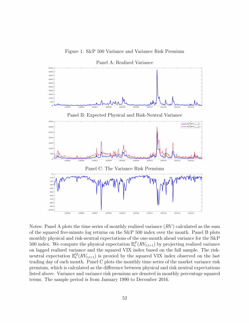
Figure 1: S&P 500 Variance and Variance Risk Premium
Panel A: Realized Variance
1992 1995 1997 2000 2002 2005 2007 2010 2012 20150
50
100
150
200
250
300
350
400
450
500
Panel B: Expected Physical and Risk-Neutral Variance
1992 1995 1997 2000 2002 2005 2007 2010 2012 20150
50
100
150
200
250
300
350
EtP[RVt,t+1]
EtQ[RVt,t+1]
Panel C: The Variance Risk Premium
1992 1995 1997 2000 2002 2005 2007 2010 2012 2015
-100
-90
-80
-70
-60
-50
-40
-30
-20
-10
0
Notes: Panel A plots the time series of monthly realized variance (RV ) calculated as the sumof the squared five-minute log returns on the S&P 500 index over the month. Panel B plotsmonthly physical and risk-neutral expectations of the one-month ahead variance for the S&P500 index. We compute the physical expectation EPt (RVt,t+1) by projecting realized varianceon lagged realized variance and the squared VIX index based on the full sample. The risk-neutral expectation EQt (RVt,t+1) is proxied by the squared VIX index observed on the lasttrading day of each month. Panel C plots the monthly time series of the market variance riskpremium, which is calculated as the difference between physical and risk neutral expectationslisted above. Variance and variance risk premium are denoted in monthly percentage squaredterms. The sample period is from January 1990 to December 2016.
52

Figure 2: Realized Covariance and the Leverage Effect
Panel A: Realized Covariance
1992 1995 1997 2000 2002 2005 2007 2010 2012 2015
-650
-600
-550
-500
-200
-150
-100
-50
0
Panel B: The Leverage Effect
1992 1995 1997 2000 2002 2005 2007 2010 2012 2015
-650
-600
-550
-500
-200
-150
-100
-50
0
Notes: Panel A plots the time series of the monthly realized covariance between the returnon the S&P 500 index and changes in its conditional variance, computed using daily datawithin each month. The time series of daily conditional variances is estimated based on theEGARCH (1,1) model using the full sample. Panel B plots the time series of the monthlyleverage effect, which is defined as the expectation of one-month ahead realized covariance.We obtain this conditional expectation of the one-month ahead realized covariance by pro-jecting realized covariance on lagged realized covariance and realized variance. The sampleperiod is from January 1990 to December 2016.
53

Figure 3: The Variance Risk Premium 1926-2016
1930 1940 1950 1960 1970 1980 1990 2000 2010-160
-140
-120
-100
-80
-60
-40
-20
0
Notes: This figure plots the time series of the variance risk premium for the S&P 500 indexin the extended sample starting in January 1926. Starting in July 1962, we use the dailyreturn time series for the S&P 500 index. Before 1962, we use the CRSP value-weightedindex as a proxy. The variance risk premium is extrapolated from estimates of the leverageeffect for the January 1926 through December 2016 sample.
54
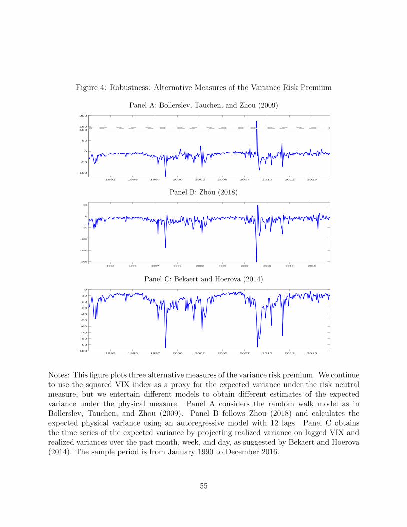
Figure 4: Robustness: Alternative Measures of the Variance Risk Premium
Panel A: Bollerslev, Tauchen, and Zhou (2009)
1992 1995 1997 2000 2002 2005 2007 2010 2012 2015
-100
-50
0
50
100150
200
Panel B: Zhou (2018)
1992 1995 1997 2000 2002 2005 2007 2010 2012 2015
-200
-150
-100
-50
0
50
Panel C: Bekaert and Hoerova (2014)
1992 1995 1997 2000 2002 2005 2007 2010 2012 2015-100
-90
-80
-70
-60
-50
-40
-30
-20
-10
0
Notes: This figure plots three alternative measures of the variance risk premium. We continueto use the squared VIX index as a proxy for the expected variance under the risk neutralmeasure, but we entertain different models to obtain different estimates of the expectedvariance under the physical measure. Panel A considers the random walk model as inBollerslev, Tauchen, and Zhou (2009). Panel B follows Zhou (2018) and calculates theexpected physical variance using an autoregressive model with 12 lags. Panel C obtainsthe time series of the expected variance by projecting realized variance on lagged VIX andrealized variances over the past month, week, and day, as suggested by Bekaert and Hoerova(2014). The sample period is from January 1990 to December 2016.
55
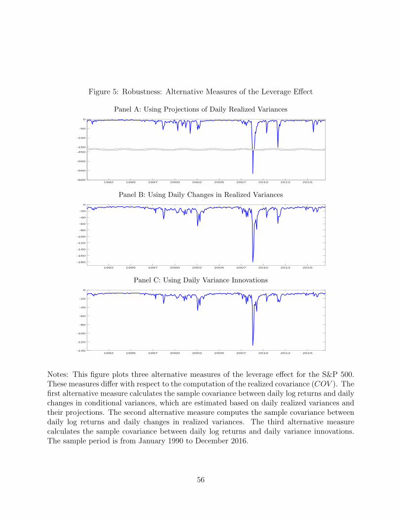
Figure 5: Robustness: Alternative Measures of the Leverage Effect
Panel A: Using Projections of Daily Realized Variances
1992 1995 1997 2000 2002 2005 2007 2010 2012 2015-600
-550
-500
-450
-150
-100
-50
0
Panel B: Using Daily Changes in Realized Variances
1992 1995 1997 2000 2002 2005 2007 2010 2012 2015
-180
-160
-140
-120
-100
-80
-60
-40
-20
0
Panel C: Using Daily Variance Innovations
1992 1995 1997 2000 2002 2005 2007 2010 2012 2015-140
-120
-100
-80
-60
-40
-20
0
Notes: This figure plots three alternative measures of the leverage effect for the S&P 500.These measures differ with respect to the computation of the realized covariance (COV ). Thefirst alternative measure calculates the sample covariance between daily log returns and dailychanges in conditional variances, which are estimated based on daily realized variances andtheir projections. The second alternative measure computes the sample covariance betweendaily log returns and daily changes in realized variances. The third alternative measurecalculates the sample covariance between daily log returns and daily variance innovations.The sample period is from January 1990 to December 2016.
56
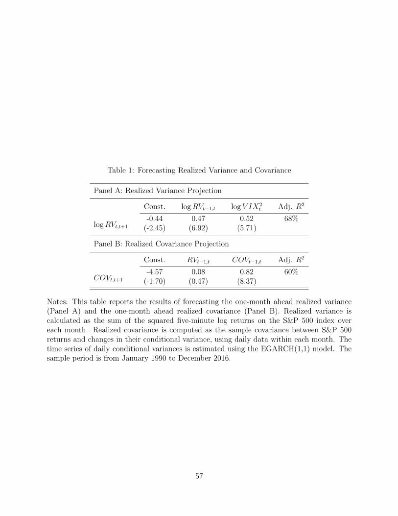
Table 1: Forecasting Realized Variance and Covariance
Panel A: Realized Variance Projection
Const. logRVt−1,t log V IX2t Adj. R2
logRVt,t+1
-0.44 0.47 0.52 68%(-2.45) (6.92) (5.71)
Panel B: Realized Covariance Projection
Const. RVt−1,t COVt−1,t Adj. R2
COVt,t+1
-4.57 0.08 0.82 60%(-1.70) (0.47) (8.37)
Notes: This table reports the results of forecasting the one-month ahead realized variance(Panel A) and the one-month ahead realized covariance (Panel B). Realized variance iscalculated as the sum of the squared five-minute log returns on the S&P 500 index overeach month. Realized covariance is computed as the sample covariance between S&P 500returns and changes in their conditional variance, using daily data within each month. Thetime series of daily conditional variances is estimated using the EGARCH(1,1) model. Thesample period is from January 1990 to December 2016.
57

Table 2: Descriptive Statistics
Panel A: Summary Statistics
N Mean Median Std. Skew. Kurt. AR(1)
RV 324 19.64 10.89 34.69 8.27 95.58 0.65ERV 324 18.62 11.91 22.26 5.58 47.22 0.77V IX2 324 37.01 27.03 33.76 3.54 18.47 0.80V RP 324 -18.39 -14.06 14.33 -2.47 8.18 0.66COV 324 -16.94 -4.68 57.51 -8.52 84.09 0.77LE 324 -16.91 -7.40 44.53 -8.53 83.52 0.78SP 324 0.66 1.03 4.16 -0.58 1.24 0.04
Panel B: Correlations
RV ERV V IX2 V RP COV LE SP
RV 1ERV 0.97 1V IX2 0.84 0.95 1V RP -0.49 -0.69 -0.88 1COV -0.93 -0.90 -0.79 0.46 1LE -0.92 -0.89 -0.78 0.46 0.99 1SP -0.36 -0.39 -0.40 0.35 0.38 0.37 1
Notes: Panel A reports the mean, median, standard deviation, skewness , kurtosis, and first-order autocorrelation for the monthly realized variance (RV ), the expected variance underthe physical measure (ERV ), the squared VIX index (V IX2), the variance risk premium(V RP ), the realized covariance (COV ), the leverage effect (LE), and the S&P 500 return(SP ). Panel B reports the correlations among these variables. The sample period is fromJanuary 1990 to December 2016.
58
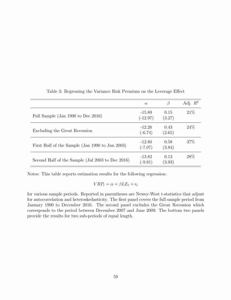
Table 3: Regressing the Variance Risk Premium on the Leverage Effect
α β Adj. R2
Full Sample (Jan 1990 to Dec 2016)-15.89 0.15 21%
(-12.97) (3.27)
Excluding the Great Recession-12.26 0.43 24%(-6.74) (2.65)
First Half of the Sample (Jan 1990 to Jun 2003)-12.80 0.58 37%(-7.07) (3.84)
Second Half of the Sample (Jul 2003 to Dec 2016)-13.82 0.13 28%(-9.81) (3.93)
Notes: This table reports estimation results for the following regression:
V RPt = α + βLEt + εt
for various sample periods. Reported in parentheses are Newey-West t-statistics that adjustfor autocorrelation and heteroskedasticity. The first panel covers the full sample period fromJanuary 1990 to December 2016. The second panel excludes the Great Recession whichcorresponds to the period between December 2007 and June 2009. The bottom two panelsprovide the results for two sub-periods of equal length.
59
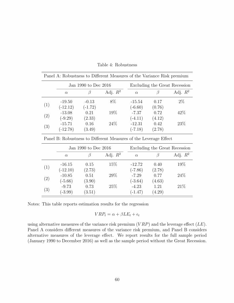
Table 4: Robustness
Panel A: Robustness to Different Measures of the Variance Risk premium
Jan 1990 to Dec 2016 Excluding the Great Recession
α β Adj. R2 α β Adj. R2
(1)-19.50 -0.13 8% -15.54 0.17 2%
(-12.12) (-1.72) (-6.60) (0.76)
(2)-13.08 0.21 19% -7.37 0.72 42%(-9.29) (2.33) (-4.11) (4.12)
(3)-15.71 0.16 24% -12.31 0.42 23%
(-12.78) (3.49) (-7.18) (2.78)
Panel B: Robustness to Different Measures of the Leverage Effect
Jan 1990 to Dec 2016 Excluding the Great Recession
α β Adj. R2 α β Adj. R2
(1)-16.15 0.15 15% -12.72 0.40 19%
(-12.10) (2.73) (-7.86) (2.78)
(2)-10.85 0.51 29% -7.29 0.77 24%(-5.66) (3.90) (-3.64) (4.63)
(3)-9.73 0.73 25% -4.23 1.21 21%
(-3.99) (3.51) (-1.47) (4.29)
Notes: This table reports estimation results for the regression
V RPt = α + βLEt + εt
using alternative measures of the variance risk premium (V RP ) and the leverage effect (LE).Panel A considers different measures of the variance risk premium, and Panel B considersalternative measures of the leverage effect. We report results for the full sample period(January 1990 to December 2016) as well as the sample period without the Great Recession.
60