The days in which we can significantly advance the science of pavement engineering throughpurely empirical approaches are over. Instead, we must turn to mechanistically-based analyses,which seek to explain the mechanisms associated with pavement deterioration. This fact isreflected in the requirement that the 2002 Guide for Design of New and Rehabilitated PavementStructures (2002 Guide, currently under development through the National Cooperative HighwayResearch Program) be based on mechanistic concepts.

This report documents the application of Long Term Pavement Performance (LTPP) data to theevaluation of mechanistically-based performance prediction procedures for jointed concretepavements. It will be of benefit to those interested in the development of mechanistically-basedperformance prediction and design procedures for jointed concrete pavements. It will be ofparticular interest to those involved in the development of the 2002 Guide.

Charles 1. Nemmers, P.E.DirectorOffice of Engineering

Research and Development

This document is disseminated under the sponsorship of the Department of Transportation in theinterest of information exchange. The United States Government assumes no liability for itscontents or use thereof. This report does not constitute a standard, specification, or regulation.

The United States Government does not endorse products or manufacturers. Trademarks ormanufacturers' names appear herein only because they are considered essential to the object ofthis document.

ee mea eport oeumentation Pa1. Report No. 2. Government Accession No. 3. Recipient's Catalog No.

FHWA-RD-98-094

4. Title and Subtitle 5. Report Date

MECHANISTIC EVALUATION OF TEST DATA June 1998FROM LTPP JOINTED CONCRETE PAVEMENT 6. Performing Organization Code

TEST SECTIONS7. Author(sl 8. Performing Organization Report No.

Y. Jane Jiang, Shiraz D. Tayabji, and Chung L. Wu

9. Performing Organization Name and Address 10. Work Unit No. (TRAISIERES Consultants, Inc.9030 Red Branch Road, Suite 210 11. Contract or Grant No.Columbia, Maryland 21045 DTFH61-95-C-00028

12. Sponsoring Agency Name and Address 13. Type of Report and Period CoveredOffice of Research & Development Final ReportFederal Highway Administration Feb 1995 - Dec 19976300 Georgetown Pike

14. Sponsoring Agency CodeMcLean, Virginia 22101-2296

15. Supplementary NotesFHWA Contracting Officer's Technical Representative (COTR): Cheryl Allen Richter, HNR-30The faulting analysis was performed by Construction Technology Laboratories (CTL), Skokie, Illinois, undera subcontract to ERES. Dr. Chung L. Wu served as the Project Manager and Mr. Paul Okamoto served asthe Administrator of the CTL subcontract.

16. Abstract

This study was conducted to assess how well some of the existing concrete pavementmechanistic-empirical based distress prediction procedures performed when used in conjunctionwith the data being collected as part of the national Long-Term Pavement Performance (LTPP)program. As part of the study, appropriate data were obtained from the National InformationManagement System (NIMS) for the GPS-3 and GPS-4 experiments. Structural analysis wasperformed for up to 140 axle load configurations for the selected test sections. Then,ILUCONand the Portland Cement Association (PCA) procedures were used to predict fatigue crackingand joint faulting damage, respectively. The computed results were compared with observedvalues.

This study has shown that, even given the many current limitations in the LTPP database, theLTPP data can be used successfully to develop better insight into pavement behavior and toimprove pavement performance.

17. Key Words 18. Distribution StatementConcrete pavement, fatigue cracking, joint No restrictions. This document is available tofaulting, LTPP, mechanistic-empirical procedures, the public through the National TechnicalNIMS, pavement distress, pavement performance, Information Service, Springfield, Virginiapavement testing, structural analysis. 22161.

19. Security Classification (of this report) 20. Security Classification (of this page) 21. No. of Pages 22. PriceUnclassified Unclassified 77

•• •APPROXIMATE CONVERSIONS TO SI UNITS APPROXIMATE CONVERSIONS FROM SI UNITS

Symbol When You Know Multiply By To Find Symbol Symbol When You Know Multiply By To Find Symbol

lENGTH lENGTHin inches 25.4 m~fimefllrs mm mm m~limefllrs 0.039 inches inft feet 0.305 meters m m meters 3.28 feet ftyd yards 0.914 meters m m meters 1.09 yards ydmi m~es 1.61 kilometers km km kilometers 0.621 miles mi

AREA AREA

in' square inches 645.2 square m~limeters mm' mm' square m~limeters 0.0016 square inches in'ftZ square feet 0.093 square meters m' m' square meters 10.764 square feet ftZycJZ square yards 0.836 square meters m' m' square meters 1.195 square yards ycJZac aaes 0.405 hectares ha ha hactares 2.47 aaes acmil square miles 2.59 square kilometers km' km' square kilometers 0.386 square miles mi'

VOLUME VOLUME

lIoz lIuidounces 29.57 milliliters mL mL milliliters 0.034 lIuidounces II ozgal galons 3.785 Uters L L Uters 0.264 gallons galft' cubic feet 0.028 cubic meters m3 mZ cubic meters 35.71 cubic feet ft'ycJZ cubic yards 0.765 cubic meters m3 mZ cubic meters 1.307 cubic yards ydl_.

III_.

NOTE: Volumes greater than 1000 I shaH be shown in mZ.

MASS MASS

oz ounces 28.35 grams g g grams 0.035 ounces ozIb pounds 0.454 kilograms kg kg kilograms 2.202 pounds IbT short tons (2000 Ib) 0.907 megagrams Mg Mg megagrams 1.103 short tons (2000 Ib) T

(or "metric ton") (or T) (or or) (or "metric ton")TEMPERATURE (exact) TEMPERATURE (exact)

DF Fahrenheit 5(F-32)19 Celcius "C "C Celcius 1.8C + 32 Fahrenheit oftemperature or (F-32Y1.8 temperature temperature temperature

IllUMINATION IllUMINATION

Ie foot-candlel 10.76 lux Ix Ix lux 0.0929 foot-candles IeII foot-t...amberts 3.426 candelalm' cdIm' cd'm' candeIaIm' 0.2919 foot-Lamberts II

FORCE and PRESSURE or STRESS FORCE and PRESSURE or STRESS

Ibf poundfon:e 4.45 newIons N N newtons 0.225 poundforce lb.IbfllnZ poundfon:e per 6.89 kiIopascall kPa kPa kiIopascals 0.145 poundforce per IbflinZ

Iqu8I8 inch square inchI

• SI is the symbol for the Intemation81 Syllllm of Units. Appropriate (Revised September 1993)rounding should be made to comply with Section 4 of ASTM E380.

CHAPTER 1 - INTRODUCTION 1The LTPP Program 2Fundamentals ofM-E Distress Modeling 3Scope of Work 5Report Organization 6

CHAPTER 2 - DATA BASE ACQUISITION 7Inventory/Section Data 7Material Characteristics 7

PCC Modulus of Elasticity, E 7PCC 28-day Flexural Strength, M, 9Poisson's Ratio ofPCC, v 10Base Elastic Modulus 11Modulus of Subgrade Reaction, k 12 ' I

LTPP Traffic Data 12Backcasting Traffic 13Cumulative Traffic Determination 15Lateral Distribution of Traffic 15

Climatic Data 16Transverse Cracking Data 16Joint Faulting Data 20Sections with Missing Data 20

CHAPTER 3 - FATIGUE CRACKING ANALYSIS 21Introduction 21Stress Calculation 21

Load Stress 22Equivalent Single-Axle Radius 23Slab Size Effect 25Tied Concrete Shoulder 26Stabilized Base 26Widened Outer Lane 27Curling Stress 28Warping Stresses ...............................•................. 29Combined Stress 29

Structural Model 30Fatigue Damage Calculation 30Correlation Between GPS-3 Fatigue Cracking and the Calculated Fatigued Damage " 31Sensitivity Analysis 32

TABLE OF CONTENTS(continued)

CHAPTER 4 - JOINT FAULTING ANAL YSIS 39Introduction 39Background 39Development of Faulting Prediction Models Based on the Erosion Factor 42Faulting at Aggregate-Interlock Joints 45Faulting at Doweled Joints 50PCC Modulus of Elasticity 54Modulus of Subgrade Reaction 54Traffic Data 54Predicted Faulting versus Measured Faulting for Aggregate-Interlock Joints 55Predicted Faulting versus Measured Faulting for Doweled Joints 55Discussion of Results 55Summary 60

CHAPTER 5 - SUMMARY AND RECOMMENDATIONS 61General Observations 61Prediction of Fatigue Cracking and Joint Faulting Using Mechanistic Procedures 61LTPP Data Issues 62

Materials Data 62Traffic Data 62Distress Data 62

Summary 63

APPENDIX A - DATA BASE FOR ANALYSIS OF TRANSVERSE CRACKING (GPS-3DATA) 69

1 An example of temperature difference distribution of a wet-freeze sectionfor an average year 18

2 An example of temperature difference distribution of a wet no-freeze sectionfor an average year . . . . . . . . . . . . . . . . . . . . . . . . . . . . . . . . . . . . . . . . . . . . . . . . . . . . . . 18

3 An example of temperature difference distribution of a dry-freeze sectionfor an average year . . . . . . . . . . . . . . . . . . . . . . . . . . . . . . . . . . . . . . . . . . . . . . . . . . . . . . 19

4 An example of temperature difference distribution of a dry no-freeze sectionfor an average year ' . . . . . . . . . . . 19

5 Axle configurations analyzed 246 Fatigue analysis results ofLTPP GPS-3 data 337 Sensitivity of the cumulative fatigue with traffic counts 338 Sensitivity plot of the fatigue damage with change of modulus of rupture 349 Sensitivity plot of the fatigue damage with change of elastic modulus of the slab 3410 Sensitivity plot of the fatigue damage with change of the PCC thermal expansion

coefficient 3511 Sensitivity plot of the fatigue damage with change of Poisson's ratio of the slab 3512 Sensitivity plot of the fatigue damage with change of subgrade k-value 3613 Faulting prediction error distribution for aggregate-interlock joints 4714 Faulting versus accumulated erosion for aggregate-interlock joints with gravel coarse

aggregate in dry region 4715 Faulting versus accumulated erosion for aggregate-interlock joints with crushed

coarse aggregate in dry region 4816 Faulting versus accumulated erosion for aggregate-interlock joints with gravel

coarse aggregate in wet region 4817 Faulting versus accumulated erosion for aggregate-interlock joints with crushed

coarse aggregate in wet region 4918 Faulting prediction error distribution for doweled joints 5219 Faulting versus accumulated erosion for doweled joints in wet region 5220 Faulting versus accumulated erosion for doweled joints in dry region 5321 Faulting prediction error distribution for aggregate-interlock joints 5622 Predicted faulting versus measured faulting for aggregate-interlock joints 5623 Faulting prediction error distribution for doweled joints 5724 Predicted faulting versus measured faulting for doweled joints 5725 Sensitivity analysis of annual traffic growth rate on computed faulting 59

LIST OF TABLES

Table Paee

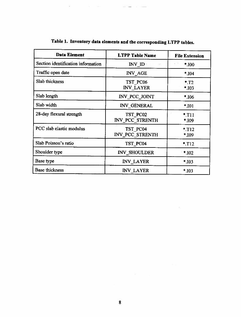
1 Inventory data elements and the corresponding LTPP tables 8

2 Thermal properties of aggregate 11

3 Selected elastic moduli for the base layer of GPS-5 sections 12

4 Summary of the GPS-3 sections with traffic monitoring data 14

5 Data elements needed for the CMS model and the corresponding LTPP tables 17

6 Summary of states surveyed 43

7 Climatic zone classification 43

8 Sensitivity of faulting to variable change for non-doweled joints 46

9 Sensitivity of faulting to variable change for doweled joints 50

Over the years, pavement engineers have been attempting to develop "rational" designprocedures for both flexible and rigid pavements. These rational procedures have focused onusing mechanistic considerations to explain the behavior of pavements under traffic andenvironmental loadings. The basic assumption of these rational procedures is that the primarypavement distresses are a result of damage induced by the state of stress, strain, or deformationthat result from traffic and environmental loadings. Under normal operating conditions, damageto the pavement occurs from a large number of repetitive traffic and environmental loadings overa period of time. Thus, each incremental loading results in some damage to the pavement, andthe cumulative effect of the damage over a period of time results in the manifestation of specificdistress, for example, fatigue cracking in asphalt concrete (AC) and portland cement concrete(PCC) pavements, rutting in AC pavements, and faulting in PCC pavements. A pavement isconsidered to have failed when the distress level (severity and extent or magnitude) reaches orexceeds a predefined acceptable level for that distress for a given category of the highway.

Since the 1950's, as techniques for analysis of pavement response to loading began to beavailable, many attempts have been made to develop these rational design procedures, nowcommonly referred to as mechanistic-empirical (M-E) procedures, to define/describe thedevelopment of specific distresses in pavements. During the late 1980's, extensive evaluationwas performed ofM-E procedures as part of the National Cooperative Highway ResearchProgram (NCHRP) 1-26 study. In addition, the proposed revision oftheAASHTO GuideforDesign of Pavements to be completed by 2002 will be based on M-E procedures. The M-Eprocedures typically involve the following steps:

1. Establishing a hypothesis for the mechanism for the development of the specificdistress. For example, the development of fatigue cracking in PCC pavements isconsidered by many to be due to repeated application of bottom tensile strain inthe PCC layer. This first step is the most critical because all the subsequent stepsdepend on the correctness of the hypothesis. The hypothesis determines the typeof analysis that needs to be conducted to compute the critical response(s) and thematerial characterization and traffic characterization needed as input for theanalysis.

2. Comprehensively characterizing materials by incorporating changes in materialproperties as a function of the state of stress (stress dependency), environmentalconditions (temperature and moisture), aging, and continual deterioration undertraffic loading.

3. Determining critical responses (stresses, strains, deformations) within thepavement layers when subjected to traffic and environmental loadings.

4. Estimating damage from each "set/condition" of traffic and environmentalloading. This is typically done using distress prediction models or transferfunctions that relate a critical structural response to distress-specific damage. Adifferent model is used for each different distress and for each pavement type.

5. Accumulating the damage over a period of time. Miner's hypothesis is generallyused to account for cumulative damage. Based on predefined relationshipsbetween the accumulated damage and amount of distress development, theamount of distress that may develop at the end of the selected service life isestimated. At this time, the selected pavement may be redesigned if the estimatedamount of distress exceeds the acceptable level or is significantly less than theacceptable level.

6. Selecting as a candidate design a pavement section that results in acceptable levelsof distresses at the end of the target service/design life. More than one sectionmay be identified as candidate designs.

Although the above steps seem simple enough, the actual process is very complexbecause of many still-undefined factors associated with pavement design and construction, trafficloading, and environmental conditions.

As part of a Federal Highway Administration (FHWA) sponsored project, work wasundertaken to use test data from the on-going Long-Term Pavement Performance (LTPP)program in conjunction with currently available M-E design procedures to assess how well theseM-E procedures perform. In essence, the LTPP test data were used to perform a reality check onthe validity of several M-E based distress prediction procedures. Under this study, existing M-Edesign procedures were used to determine cumulative damage in relation to a specific distress ineach applicable LTPP test section. The estimated distress was compared with predicted distress.In addition, an attempt was made to develop calibrated distress models that relate theaccumulated damage to the observed level of distress.

This report presents the results of the study applicable to jointed PCC test sections fromthe LTPP program. In the subsequent sections, details are presented on the LTPP program, theLTPP data used in the study, and the procedures undertaken to compute the cumulative damage.

The LTPP program is a 20-year program established under the now-completed StrategicHighway Research Program (SHRP). The first 5 years of the LTPP program (mid-1987 to mid-1992) were funded under the SHRP funding; since mid-1992, FHW A has assumed themanagement and funding of the LTPP program. Although the LTPP program was conceived tomeet many needs of the pavement engineering community, one major objective was to develop anational pavement performance data base that could be used to develop and/or validate pavementdesign procedures. The study reported here was aimed at fulfilling that objective.

The LTPP program is collecting information on the long-term performance of variouspavement structures under a range of traffic loadings, climatic factors, and subgrade soils. TheLTPP program includes two fundamental classes of studies: the General Pavement Studies(GPS) and the Specific Pavement Studies (SPS). The GPS experiments are a series of selectedin-service pavement studies structured to develop a comprehensive national pavementperformance data base. These studies are restricted to pavements that incorporate materials and

designs representing good engineering practice and that are in common use across the UnitedStates and Canada. Studies included in GPS are:!

First Performance PeriodGPS-l Asphalt Concrete (AC) on Granular BaseGPS-2 AC on Bound BaseGPS-3 Jointed Plain ConcreteGPS-4 Jointed Reinforced ConcreteGPS-5 Continuously Reinforced Concrete

OverlaysGPS-6GPS-7GPS-9

AC Overlays on ACAC Overlays on Portland Cement Concrete PavementsUnbonded PCC Overlays on PCC Pavements

Specific details on the GPS-3 and GPS-4 experiments as pertaining to the study reportedhere are provided in later sections of the report. The SPS program involves the study of speciallyconstructed, maintained, or rehabilitated pavement sections incorporating a controlled set ofexperimental design and construction features. Test data from the SPS experiments were notincluded in this study. As such, no additional discussion on the SPS experiments is providedhere.

As part of the LTPP program, an extensive data collection effort has been under waysince about 1989. These data types are classified within the LTPP program as follows:

1. Inventory2. Materials Testing3. Climatic4. Monitoring5. Traffic6. Seasonal

In addition, as appropriate, maintenance, rehabilitation, and construction data are alsocollected.

The M-E distress modeling approach for PCC pavements involves the followingelements:

1. A structural analysis model that can consider the geometry of the pavement, theloading condition (multiple wheel loads), and load transfer effectiveness at jointsand that is capable of reliably determining the critical responses appropriate to thedistress being considered. For PCC pavements, most of the M-E distress modelwork has been done using plate on elastic (liquid or Winkler) foundationapproach.

2. A fairly reliable estimate of traffic loading. Advanced M-E procedures considerthe axle loading spectra while other models are based on use of equivalent loading(e.g., ESAL) in which case all loadings are transformed into a single load typeusing load equivalency concepts. The use of equivalent traffic loading limits theusefulness of many of these models in developing rational design procedures.

The traffic loading data may need to be available on a seasonal basis and,in the case of concrete pavements, on a diurnal basis as well as by lateralplacement along the width of the traffic lane.

3. A fairly reliable estimate of seasonal climatic conditions to account for changes inmaterial properties and, in the case of concrete pavements, to also account for theeffect of temperature differentials within the concrete slab on curling stresses.

4. Comprehensive material characterization. The PCC material properties need to becharacterized in terms of aging. For PCC materials, seasonal effects are notconsidered. The granular material properties need to be characterized in terms ofstress dependency and in terms of seasonal variation as a result of seasonalmoisture and temperature variations within these materials. For example, thespring-thaw characterization for fine-grai~ed materials is very important.

5. Availability of "calibrated" mechanistic distress models or transfer functions thatincorporate mechanistic responses. The general approach has been to develop"absolute" models based on laboratory testing and laboratory failure criteria and toextrapolate these laboratory models to field conditions using a shift factor toaccount for different levels of distress development and other unaccountablefactors. For example, for PCC fatigue cracking, early models were developed onthe basis of laboratory testing and the first crack initiation as the failure criterion.These models were then expanded to account for field observations and toincorporate different levels of fatigue cracking (e.g., in terms of number of slabpanels exhibiting cracking).

6. Acceptance of Miner's fatigue damage hypothesis. Miner's hypothesis allows amethod for combining various levels of damage from the combination of trafficand environmental loadings. Miner's hypothesis states that the structural fatiguedamage is cumulative and that a structure's fatigue life is finite, defined by theallowable number of load applications prior to failure. Each load applicationconsumes a small amount of fatigue life. When the actual load applications equalthe number of allowable load applications, the fatigue damage is 1.0 or 100percent and failure occurs. Miner's hypothesis is typically stated as follows:

~ n.Fatigue Damage, Df = LJ-'N;

where: Dfnj

Nj

Cumulative fatigue damage.Actual number of load applications of load group i.Allowable number of load applications to failure of load group i.

In an ideal M-E procedure, damage (in relation to a specific distress) should bedetermined as follows:

Damage ij/d = f (eij/d)and

eij/d = f (Ej/d)

Critical structural response in the pavement that is considered to be apredictor of the distress under consideration for the ith axle group at the jthtime period of the kth month of the Ah year.Modulus of elasticity of each layer of the pavement system at the jth timeperiod of the kth month of the Ah year.

Thus, a major consideration in developing and using M-E procedures is the appropriatecharacterization of Ejkl for each of the pavement layer. Our capability for realistically modelingpavement behavior has seen much progress in the last few decades. However, the capability torealistically consider material characterization (e.g., Ejkl) for the pavement layers remains lessthan desired because of the lack of knowledge on how to realistically account for seasonaleffects, spatial variability, and effects of deterioration due to traffic loading and environment.

It should be noted that the above steps are applicable for use of the M-E distress modelsfor design of new/rehabilitated pavements or for checking such designs. The application of theM-E distress models to existing pavements to further validate/calibrate the models creates anentirely different set of problems. Such an effort requires very reliable data on materialproperties, pavement section layering, past traffic loading history, past environmental conditions,and distress manifestation.

The validation/calibration process involves predicting cumulative damage or distress andcomparing the predicted distress to observed distress. The study reported here was aimed atvalidating or calibrating the distress prediction models for transverse fatigue cracking in jointedplain PCC pavements and for faulting in jointed PCC pavements.

The overall objective of the study was to assess how well some of the existing M-E baseddistress prediction procedures performed when used in conjunction with the LTPP data.Specifically, it was decided to assess the transverse cracking prediction procedure developed atthe University of Illinois as part of the NCHRP 1-26 study and the joint faulting predictionprocedure developed by the Portland Cement Association.

• Use of deflection data to backcalculate the pavement layer moduli - an importantinput to structural evaluation. The base/subbase/subgrade was modeled as a liquidfoundation and was therefore characterized in terms of the modulus of subgradereaction, k.

• Use of an algorithm based on finite-element analysis of jointed slabs on elasticfoundation to calculate the critical responses. The horizontal tensile strain at thebottom of the PCC layer at mid-slab edge was used as a predictor of fatiguecracking and the deflections at joints were used as a predictor of rutting.Pavement response was calculated for each load level and axle category.

• Existing transfer functions (those developed by the University of Illinois and thePortland Cement Association) were then used to predict the damage associatedwith each load level. The damage was summed over all load groups and over theentire service life of the pavement. The resulting total damage was then comparedwith the observed pavement distresses to ascertain if there was a reasonableagreement between the observed and predicted distress levels.

As discussed, this study was aimed at using LTPP data to assess the applicability ofseveral existing M-E analysis procedures. Specifically, the University of Illinois procedure forpredicting the development of fatigue cracking and the Portland Cement Association procedurefor predicting the development of faulting in jointed PCC pavements were considered. Chapter 2details the process used to develop the necessary data needed for the study using the LTPP database. In chapter 3, analysis results are presented for assessment of the University of Illinois(NCHRP 1-26) fatigue cracking prediction procedure. In chapter 4, analysis results are presentedfor assessment of the Portland Cement Association's joint faulting prediction procedure. Chapter5 presents a summary of findings and provides a discussion on improvements that need to bemade to further advance the reliability ofM-E procedures using LTPP data.

The LTPP data used in the analysis reported here were obtained from the NationalInformation Management System (NIMS) during February 1996 (Release 6.0 data). The datawere the most recent version of the data release as of the date of this study. The NIMS data arecategorized into seven modules: inventory, environment, material testing, monitoring,maintenance, rehabilitation, and traffic. In each module, the data are stored in tables that containa related set of data elements. This section briefly discusses the data elements used in theanalysis, the specific tables from which the data were obtained, the manipulations performed onthe data, and the test sections that were excluded from the analysis because of the lack of data.

Inventory data include general information about each LTPP section, such as sectionidentification, pavement construction date, original design, etc. The key inventory data elementswith the corresponding LTPP table names and file extensions used in NIMS are shown in table 1.

Most inventory data variable values were retrieved directly from the NIMS data baseexcept for the slab thickness. If slab thickness data were available from the concrete cores takenfrom the field, the average core thickness was used. Otherwise, the thickness value from theinventory table was used.

The material properties that are typically used in the mechanistic evaluation of transversefatigue cracking are listed below:

'. PCC modulus of elasticity.• PCC 28-day flexural strength.• PCC Poisson's ratio.• PCC coefficient of thermal expansion.• Stabilized base modulus of elasticity.• Modulus of subgrade reaction, k.

Backcalculated slab elastic moduli for the LTPP sections were available from a previousstudy conducted by ERES Consultants, Inc., under FHW A Contract No. DTFH61-94-C-00218.However, because of too many unreasonably high values (greater than 55,000 MPa) from thebackcalculation results, these were not used in this study. The following procedure therefore wasadopted to estimate the concrete elastic modulus for each section:

1. Obtain the elastic modulus from LTPP data table TST_PC04 (file extension*.TI2). The test results were obtained in the laboratory using field cores. This

Data Element LTPP Table Name File Extension

Section identification information INV ID *.100-Traffic open date INV AGE *.104

Slab thickness TST PC06 *.T2INV LAYER *.103

Slab length INV PCC JOINT *.106- -Slab width INV GENERAL *.101

28-day flexural strength TST PC02 *.TllINV PCC STRENTH *.109- -

PCC slab elastic modulus TST PC04 *.TI2INV PCC STRENTH *.109- -

Slab Poisson's ratio TST PC04 *.TI2

Shoulder type INV SHOULDER *.102

Base type INV LAYER *.103

Base thickness INV LAYER *.103

applies to 129 GPS-3 and GPS-4 sections out of the total of 192 GPS-3 and GPS-4 sections.

2. If laboratory test results were not available, then the elastic modulus wasextrapolated using the 28-day flexural strength values obtained from the tableINV _PCC_STRENGTH (file extension •••.109). Fifteen sections fall into thiscategory.

3. If neither of the above two options were available, a value of27,580 MPa wasassigned to the section. This value has typically been used to represent the elasticmodulus for pavement concrete. The default value of27,580 MPa was used for48 sections.

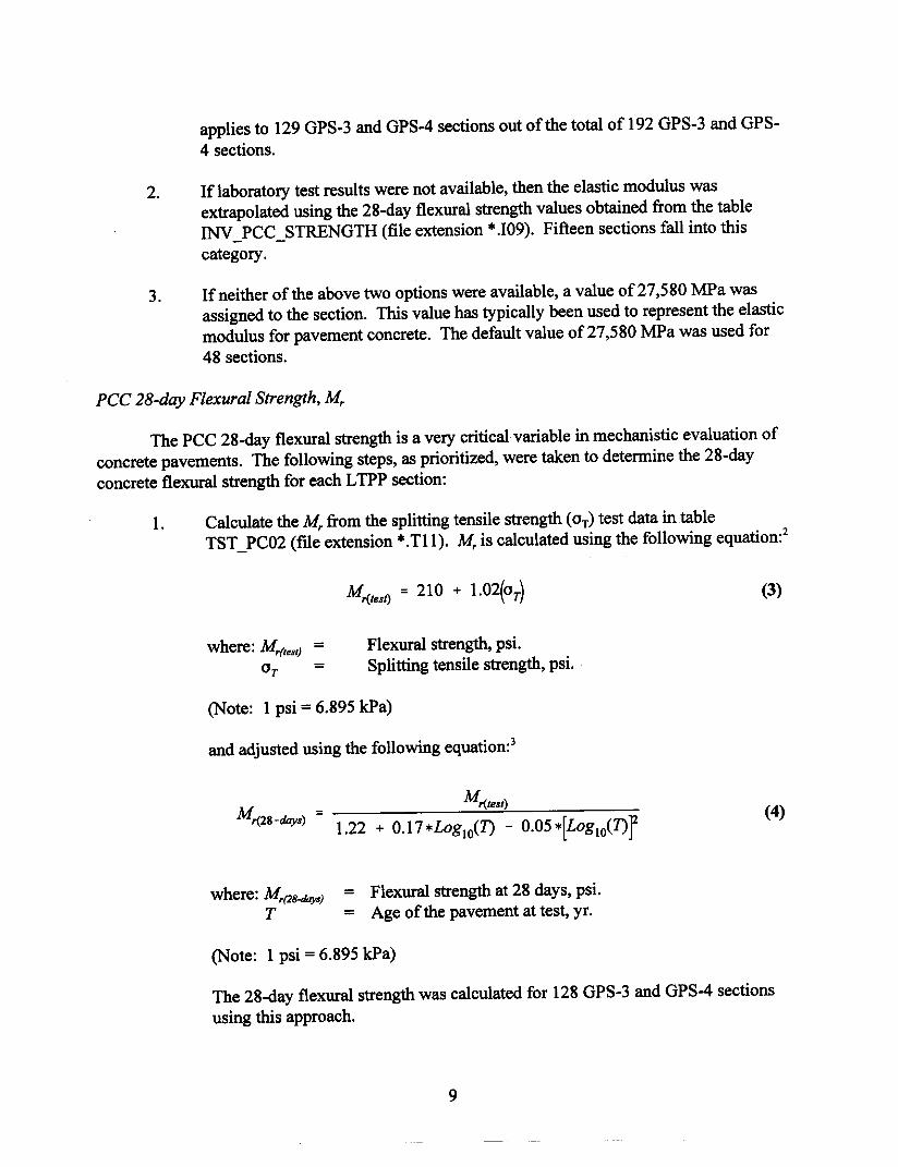
The PCC 28-day flexural strength is a very critical variable in mechanistic evaluation ofconcrete pavements. The following steps, as prioritized, were taken to determine the 28-dayconcrete flexural strength for each LTPP section:

1. Calculate the Mr from the splitting tensile strength (OT) test data in tableTST_PC02 (file extension •••.Tll). Mr is calculated using the following equation:2

Mr(leS/) = 210 + 1.02(0T)

where: Mr(,e8t) =or

Flexural strength, psi.Splitting tensile strength, psi.

where: M,(28-days)

T= Flexural strength at 28 days, psi.= Age of the pavement at test, yr.

The 28-day flexural strength was calculated for 128 GPS-3 and GPS-4 sectionsusing this approach.

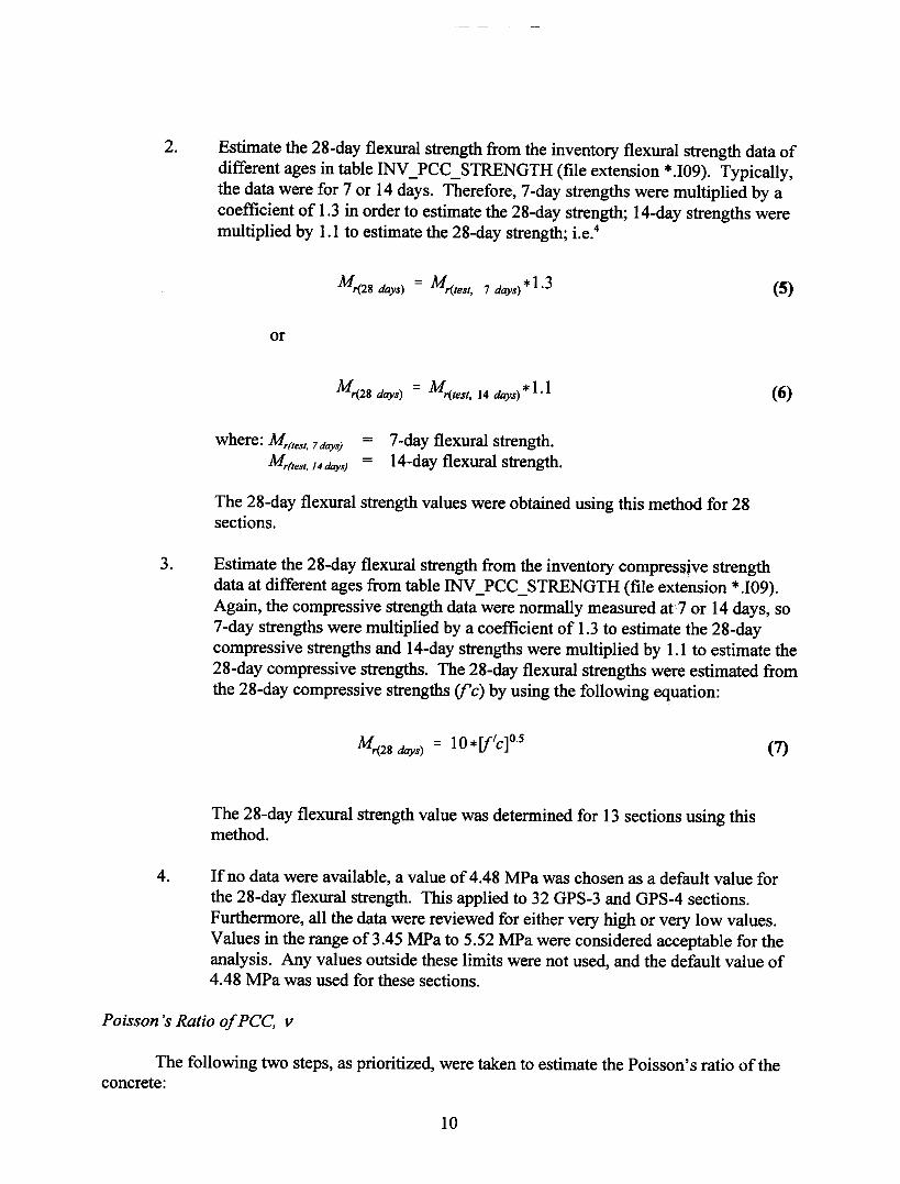
2. Estimate the 28-day flexural strength from the inventory flexural strength data ofdifferent ages in table INV_PCC_STRENGTH (file extension *.109). Typically,the data were for 7 or 14 days. Therefore, 7-day strengths were multiplied by acoefficient of 1.3 in order to estimate the 28-day strength; 14-day strengths weremultiplied by 1.1 to estimate the 28-day strength; i.e.4

Mr(28 days) = Mr(test, 7 days)*1.3

Mr(28 days) = Mr(test, 14 days)*1.1

where: Mr(test, 7 days)

M,.(test, I4 days)

= 7-day flexural strength.= 14-day flexural strength.

The 28-day flexural strength values were obtained using this method for 28sections.

3. Estimate the 28-day flexural strength from the inventory compressive strengthdata at different ages from table INV_PCC_STRENGTH (file extension *.109).Again, the compressive strength data were normally measured at7 or 14 days, so7-day strengths were multiplied by a coefficient of 1.3 to estimate the 28-daycompressive strengths and 14-day strengths were multiplied by 1.1 to estimate the28-day compressive strengths. The 28-day flexural strengths were estimated fromthe 28-day compressive strengths (f'e) by using the following equation:

M = 10*[fle]0.5r(28 days)

The 28-day flexural strength value was determined for 13 sections using thismethod.

4. If no data were available, a value of 4.48 MPa was chosen as a default value forthe 28-day flexural strength. This applied to 32 GPS-3 and GPS-4 sections.Furthermore, all the data were reviewed for either very high or very low values.Values in the range of3.45 MPa to 5.52 MPa were considered acceptable for theanalysis. Any values outside these limits were not used, and the default value of4.48 MPa was used for these sections.

The following two steps, as prioritized, were taken to estimate the Poisson's ratio of theconcrete:

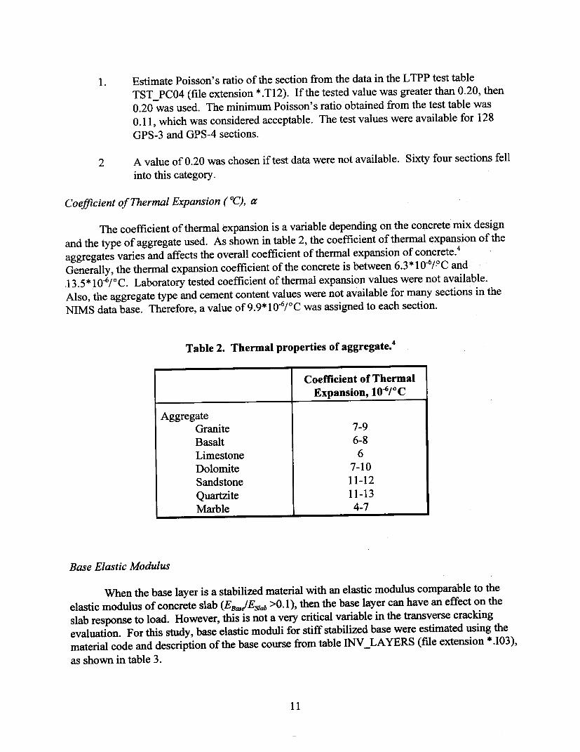
1. Estimate Poisson's ratio of the section from the data in the LTPP test tableTST_PC04 (file extension *.TI2). If the tested value was greater than 0.20, then0.20 was used. The minimum Poisson's ratio obtained from the test table was0.11, which was considered acceptable. The test values were available for 128GPS-3 and GPS-4 sections.

2 A value of 0.20 was chosen iftest data were not available. Sixty four sections fellinto this category.

The coefficient of thermal expansion is a variable depending on the concrete mix designand the type of aggregate used. As shown in table 2, the coefficient of thermal expansion of theaggregates varies and affects the overall coefficient of thermal expansion of concrete.4Generally, the thermal expansion coefficient of the concrete is between 6.3*10..(i/PCand.l3.5*1O-6/oC. Laboratory tested coefficient of thermal expansion values were not available.Also, the aggregate type and cement content values were not available for many sections in theNIMS data base. Therefore, a value of9.9*1O-6/oC was assigned to each section.

Coefficient of ThermalExpansion,lO-6;oC

AggregateGranite 7-9Basalt 6-8Limestone 6Dolomite 7-10Sandstone 11-12Quartzite 11-13Marble 4-7

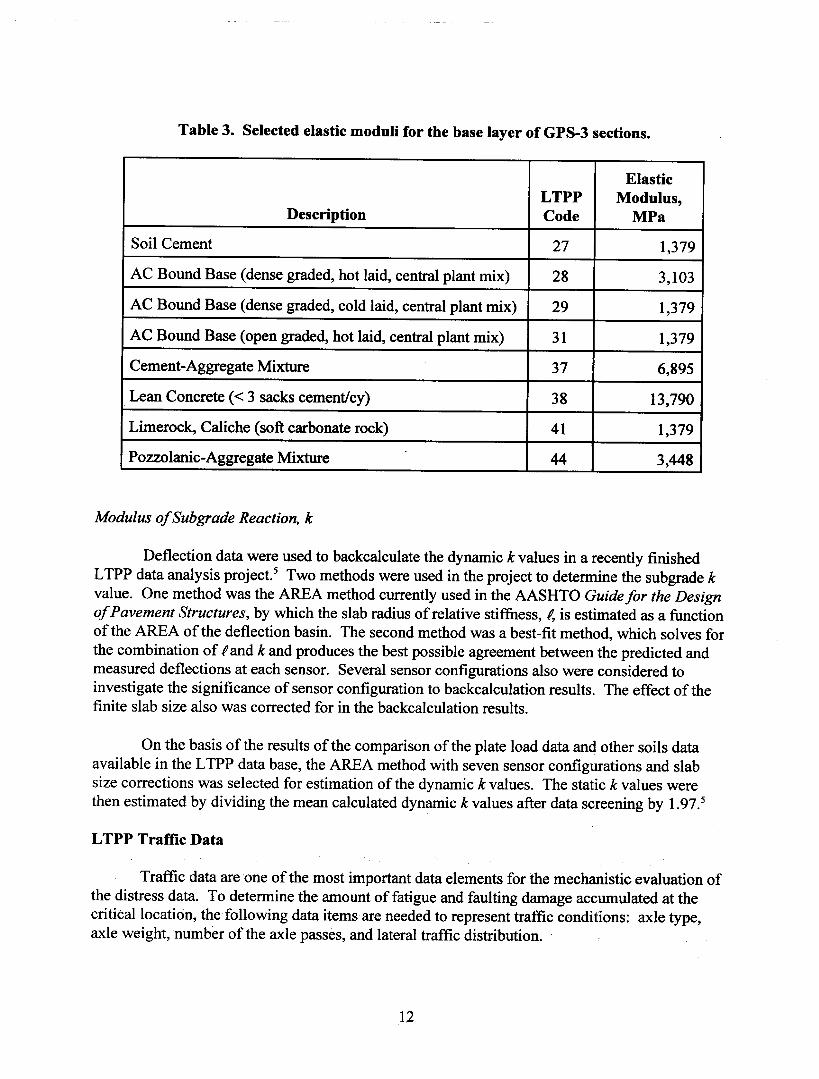
When the base layer is a stabilized material with an elastic modulus comparable to theelastic modulus of concrete slab (EBas)Eslab >0.1), then the base layer can have an effect on theslab response to load. However, this is not a very critical variable in the transverse crackingevaluation. For this study, base elastic moduli for stiff stabilized base were estimated using thematerial code and description of the base course from table INV_LAYERS (file extension *.103),as shown in table 3.

ElasticLTPP Modulus,

Description Code MPa

Soil Cement 27 1,379

AC Bound Base (dense graded, hot laid, central plant mix) 28 3,103

AC Bound Base (dense graded, cold laid, central plant mix) 29 1,379

AC Bound Base (open graded, hot laid, central plant mix) 31 1,379

Cement-Aggregate Mixture 37 6,895

Lean Concrete « 3 sacks cement/cy) 38 13,790

Limerock, Caliche (soft carbonate rock) 41 1,379

Pozzolanic-Aggregate Mixture 44 3,448

Deflection data were used to backcalculate the dynamic k values in a recently finishedLTPP data analysis project. 5 Two methods were used in the project to determine the subgrade kvalue. One method was the AREA method currently used in the AASHTO Guide for the Designof Pavement Structures, by which the slab radius of relative stiffness, f, is estimated as a functionof the AREA of the deflection basin. The second method was a best-fit method, which solves forthe combination of f and k and produces the best possible agreement between the predicted andmeasured deflections at each sensor. Several sensor configurations also were considered toinvestigate the significance of sensor configuration to backcalculation results. The effect of thefinite slab size also was corrected for in the backcalculation results.

On the basis of the results of the comparison of the plate load data and other soils dataavailable in the LTPP data base, the AREA method with seven sensor configurations and slabsize corrections was selected for estimation of the dynamic k values. The static k values werethen estimated by dividing the mean calculated dynamic k values after data screening by 1.97.5

Traffic data are one of the most important data elements for the mechanistic evaluation ofthe distress data. To determine the amount offatigue and faulting damage accumulated at thecrititallocation, the following data items are needed to represent traffic conditions: axle type,axle weight, number of the axle passes, and lateral traffic distribution.

Intensive efforts are being made to obtain quality traffic data for the LTPP studies. Sitemonitored traffic data for some sections have recently become available, including AutomaticVehicle Classification (AVC) and Weight-In-Motion (WIM) data. Only the WIM data were usedin this study. The data relevant to this study are included in the following two tables:

TRF _MONITOR_AXLE_DISTRIB (file extension *.F04)TRF_MONITOR_BASIC_INFO (file extension *.F01)

The first table provides information on the axle type, axle weight, and the total number ofaxles passes for the monitoring year; the second table includes the information on the number ofdays with WIM monitoring in a given year. The total count is extrapolated based on the numberof passes on the WIM monitoring days. Some sections had only 1 year of traffic monitoring data,while others had 2 or 3 years of traffic monitoring data. The monitoring year with the highestnumber of days with WIM data was selected to represent the traffic condition of the section inone specific year. This was generally the last year ofthe traffic monitoring data available. Thereare 140 axle load/type categories for each section. The axle categories include single, tandem,tridem, and four-axle assemblies.

For the fatigue cracking evaluation study, a total of 52 jointed plain concrete pavement(JPCP) sections from a total of 129 sections in the GPS-3 experiment had at least 1 day of trafficmonitoring data in 1 year. Table 4 provides a list of sections with traffic monitoring data for theyear with the highest number of days of WIM data.

Since the traffic data obtained from the LTPP NIMS data base were available only for afew years, the traffic data for the remaining years had to be backcasted to the year when thepavement was opened to traffic in order to estimate the cumulative traffic.

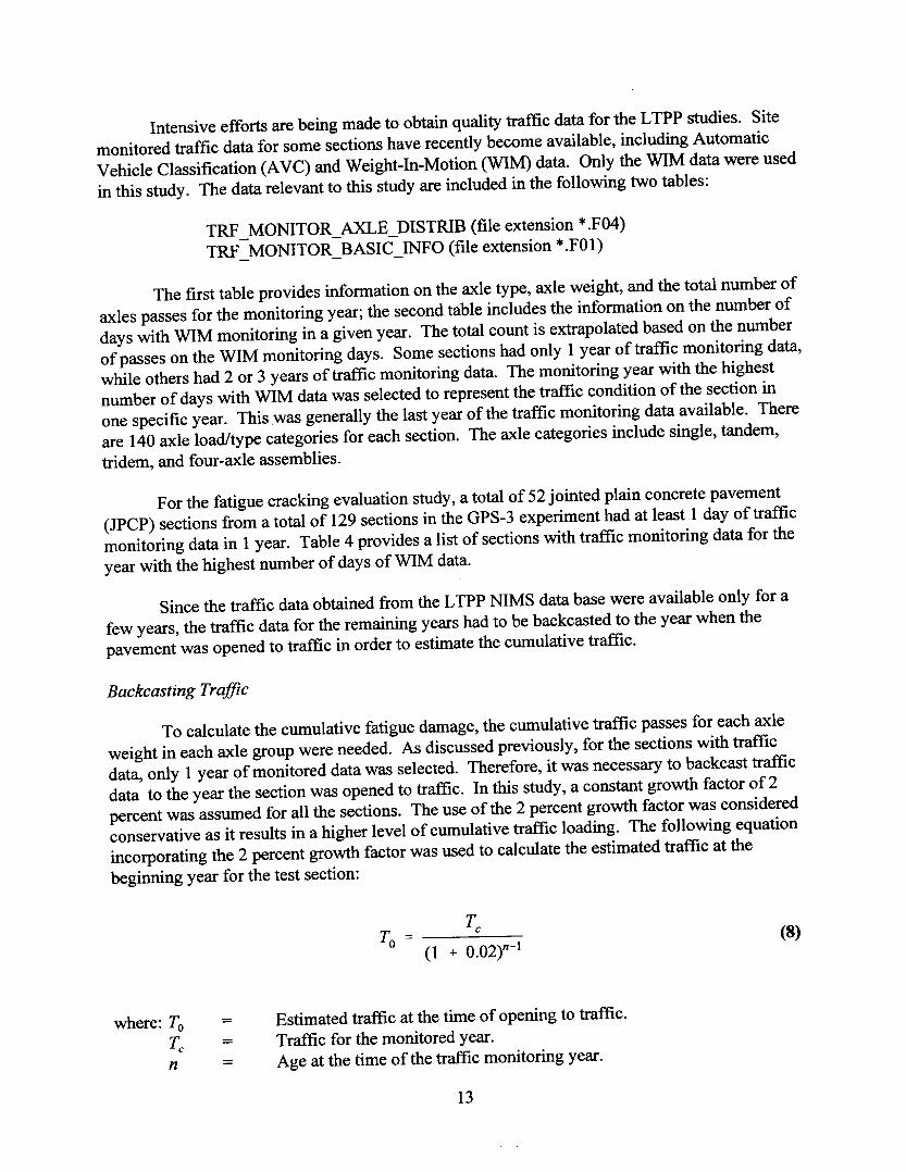
To calculate the cumulative fatigue damage, the cumulative traffic passes for each axleweight in each axle group were needed. As discussed previously, for the sections with trafficdata, only 1 year of monitored data was selected. Therefore, it was necessary to backcast trafficdata to the year the section was opened to traffic. In this study, a constant growth factor of 2percent was assumed for all the sections. The use of the 2 percent growth factor was consideredconservative as it results in a higher level of cumulative traffic loading. The following equationincorporating the 2 percent growth factor was used to calculate the estimated traffic at thebeginning year for the test section:

where: ToTc

n

Estimated traffic at the time of opening to traffic.Traffic for the monitored year.Age at the time of the traffic monitoring year.

State SHRPID Traffic Monitorin2 Year Number of Days with WIM Data5 3011 1993 426 3030 1992 296 3042 1992 668 3032 1993 16112 3804 1993 1412 3811 1993 1412 4000 1993 34312 4057 1993 33312 4059 1993 31512 4109 1993 31712 4138 1993 34313 3015 1993 613 3018 1993 318 3002 1993 16818 3003 1993 22718 3030 1993 30418 3031 1993 13519 3006 1993 5919 3009 1993 619 3028 1993 520 3013 1992 520 3015 1993 20121 3016 1993 14626 3068 1993 31826 3069 1993 31727 3003 1993 21927 3013 1992 36229 5393 1993 731 3018 1993 931 3023 1993 931 3028 1993 731 3033 1993 632 3010 1990 2032 3013 1992 632 7084 1992 1438 3005 1993 16838 3006 1993 7940 4160 1993 3140 4162 1993 2942 1623 1991 542 3044 1993 346 3012 1993 13053 3011 1993 35153 3013 1993 34353 3014 1992 31453 3019 1992 32453 3812 1993 36253 3813 1993 36553 7409 1993 33083 3802 1993 20589 3015 1993 125R9 1016 1992 172

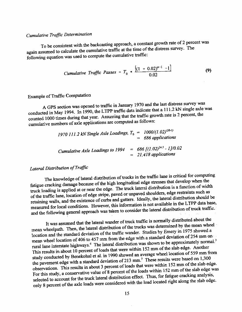
To be consistent with the backcasting approach, a constant growth rate of2 percent wasagain assumed to calculate the cumulative traffic at the time of the distress survey. Thefollowing equation was used to compute the cumulative traffic:

1(1 + 0.02)n-l I}Cumulative Traffic Passes = To * -

0.02

A GPS section was opened to traffic in January 1970 and the last distress survey wasconducted in May 1994. In 1990, the LTPP traffic data indicate that a 111.2 kN single axle wascounted 1000 times during that year. Assuming that the traffic growth rate is 2 percent, thecumulative numbers of axle applications are computed as follows:

1970111.2 kN Single Axle Loadings, To = 1000/(1.02/20-1)

= 686 applications

Cumulative Axle Loadings to 1994 = 686 [(1.02/4.5 - 1]/0.0221,418 applications

The knowledge of lateral distribution of trucks in the traffic lane is critical for computingfatigue cracking damage because of the high longitudinal edge stresses that develop when thetruck loading is applied at or near the edge. The truck lateral distribution is a function of widthof the traffic lane, location of edge stripe, paved or unpaved shoulders, edge restraints such asretaining walls, and the existence of curbs and gutters. Ideally, the lateral distribution should bemeasured for local conditions. However, this information is not available in the LTPP data base,and the following general approach was taken to consider the lateral distribution of truck traffic.

It was assumed that the lateral wander of truck traffic is normally distributed about themean wheelpath. Then, the lateral distribution of the trucks was determined by the mean wheellocation and the standard deviation of the traffic wander. Studies by Emery in 1975 showed amean wheel location of 406 to 457 mm from the edge with a standard deviation of 254 mm onrural lane interstate highways.6 The lateral distribution was shown to be approximately normal. 3

This results in about 10 percent ofloads that were within 152 mm of the slab edge. Anotherstudy conducted by Benekohal et al. in 1990 showed an average wheel location of559 mm fromthe pavement edge with a standard deviation of213 mm.7 These results were based on 1,300observations. This results in about 3 percent of loads that were within 152 mm of the slab edge.For this study, a conservative value of 8 percent of the loads within 152 mm of the slab edge wasselected to account for the truck lateral distribution effect. Thus, for fatigue cracking analysis,only 8 percent of the axle loads were considered with the load located right along the slab edge.

Climate is another important factor that affects pavement performance. With respect tofatigue cracking, the most significant factor is the temperature differential or thermal gradientbetween the top and the bottom of the slab and the moisture in the slab. The thermal gradient canbe either positive (i.e., the top of the slab is warmer than the bottom, or negative, with the top ofthe slab cooler than the bottom). A positive thermal gradient causes the top to curl downward,which is resisted by the support. This creates restraint tensile stress at the bottom of the slab withthe maximum stress level midway between the joints. A negative thermal gradient causes thecomers of the slab to curl upward, and this is resisted by the weight of the slab. This results intensile stress at the top of the comer region of the slab. The downward curling of the slab causedby the positive thermal gradient adds to the loading stress caused by the traffic. This can increasethe critical stresses in the concrete slab dramatically, especially with large positive thermalgradients. The fatigue damage caused during the negative temperature gradients is negligible asthe curling stresses subtract from the load stresses. Therefore, only the positive thermal gradientswere considered in this study.

The temperature gradient in the pavement slabs change continuously through the day.The main factors affecting the magnitude of temperature gradients are air temperature, windspeed, and the amount oftime the slabs are exposed to the sun. To adequately account for theeffect of temperature gradients, hourly temperature gradient data for the entire year from therepresentative years were needed. The Climatic-Materials-Structural (CMS) pavement analysisprogram was used to generate the needed data from the monthly derived climatic data in theLTPP data base.8 The CMS model has been validated and has been shown to predicttemperatures in pavement slabs reasonably well. The CMS model calculates the thermal gradientwith depth considering air temperature, radiation heating and cooling, convection, cloud cover,wind speed, and material properties. From the LTPP climatic data base, the variables used tocalculate the thermal gradients using the CMS model are shown in table 5.

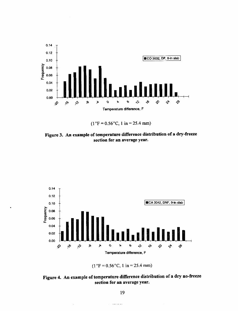
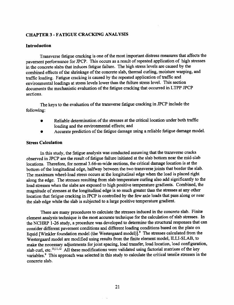
Examples of the histograms of temperature differential versus frequency of occurrence inpercent time of the year for a few sections are given in figures 1 through 4. Average monthlymaximum temperature and average monthly minimum temperature were available for most ofthe JPCP sections. However, only 56 sections out of a total of 129 sections in the GPS-3experiment had percent sunshine data and only 81 sections had wind speed data. For the sectionswithout either percent sunshine data or wind speed data, the average value of these parametersfor other sections in the same State or the surrounding States were used instead.

The manual transverse cracking data are stored in the table MON_DIS_JPCC_REV (fileextension * .M08). The data elements used in the evaluation are TRANS_CRACK _NO _L,TRANS _CRACK_NO _M, and TRANS_ CRACK_NO _H. The parameter of interest is thepercent slabs cracked in the 152.4-m section, which can be calculated as:

Data Element LTPP Table Name File Extension

Average monthly maximum ENV MONTHLY PARAMETER *.E03- -temperature (1959 to 1989)

Average monthly minimumtemperature (1959 to 1989)

Average monthly wind speed(1959 to 1989)

Average monthly percentsunshine(1959 to 1989)

PCC slab thickness TST PC06 *.T2INV LAYER *.103

Latitude INV ID *.100

0.10

~5j 0.08::::J10.06

0.04

I-MO 5393, WF. 8-ln slab I

Figure 1. An example of temperature difference distribution of a wet-freezesection for an average year.

0.16

0.14

0.12 ,- FL 3811, WNF, 9-ln slab I~ 0.10cCDt 0.08

u. 0.06

0.04

0.02

0.00

Figure 2. An example of temperature difference distribution of a wet no-freezesection for an average year.

IIIco 3032, OF, 8-in slab I~55 0.08~tr~ 0.06u.

Figure 3. An example of temperature difference distribution of a dry-freezesection for an average year.

IIICA 3042, ONF, 9-in slab I~55 0.08~~ 0.06u.

Figure 4. An example of temperature difference distribution of a dry no-freezesection for an average year.

% slabs cracked = (Total TRANS CRACKED NO) * average joint spacing, m- - 152.4

where: TOTAL TRANS CRACK NO = TRANS CRACK NO L +- --TRANS CRACK NO M +- --TRANS CRACK NO H.- --

For the sections with traffic data but no manual transverse cracking data, thephotographic distress data in the table MON_DIS_PADIAS_JC (file extension *.M17) wereused. No attempt was made to differentiate between midslab and non-midslab transversecracking or random cracking (construction related) as these data were not readily available. Itwas assumed that a very low amount, if any, of random cracking was present in the GPS-3sections.

The joint faulting data were derived from the table MON_DIS_JPCC_FAULT (fileextension * .M09). The table lists the values for joint faulting at the comer and at the wheelpathat each joint. The values used in the analysis were the comer values, averaged along the l52.4-mlength of the section.

The total number of GPS-3 sections is 129 and the total number of GPS-4 sections is 68.Only GPS-3 sections were used for the analysis of fatigue cracking. For joint faulting analysis,both GPS-3 and GPS-4 were used. However, as discussed, many sections were missing key datasuch as traffic and distress data. These sections were not used in the analysis. For analysis offatigue cracking, data from 52 sections (with traffic data availability) were used. For the analysisof faulting data, data from 57 sections (20 with aggregate interlock joints and 37 with doweledjoints) were used.

It should be clear from the information presented in this chapter that LTPP test sectionshave zero utility if any of the critical data elements are missing or are of questionable quality.

Transverse fatigue cracking is one of the most important distress measures that affects thepavement performance for JPCP. This occurs as a result of repeated application of high stressesin the concrete slabs that induces fatigue failure. The high stress levels are caused by thecombined effects of the shrinkage of the concrete slab, thermal curling, moisture warping, andtraffic loading. Fatigue cracking is caused by the repeated application of traffic andenvironmental loadings at stress levels lower than the failure stress level. This sectiondocuments the mechanistic evaluation of the fatigue cracking that occurred in LTPP JPCPsections.

The keys to the evaluation of the transverse fatigue cracking in JPCP include thefollowing:

• Reliable determination of the stresses at the critical location under both trafficloading and the environmental effects; and

• Accurate prediction of the fatigue damage using a reliable fatigue damage model.

In this study, the fatigue analysis was conducted assuming that the transverse cracksobserved in JPCP are the result of fatigue failure initiated at the slab bottom near the mid-slablocations. Therefore, for normal3.66-m-wide sections, the critical damage location is at thebottom of the longitudinal edge, halfway between the two transverse joints that border the slab.The maximum wheel-load stress occurs at the longitudinal edge when the load is placed rightalong the edge. The stresses resulting from slab temperature curling also add significantly to theload stresses when the slabs are exposed to high positive temperature gradients. Combined, themagnitude of stresses at the longitudinal edge is so much greater than the stresses at any otherlocation that fatigue cracking in JPCP is controlled by the few axle loads that pass along or nearthe slab edge while the slab is subjected to a large positive temperature gradient.

There are many procedures to calculate the stresses induced in the concrete slab. Finiteelement analysis technique is the most accurate technique for the calculation of slab stresses. Inthe NCHRP 1-26 study, a procedure was developed to determine the structural responses that canconsider different pavement conditions and different loading conditions based on the plate onliquid [Winkler foundation model (the Westergaard model)].9 The stresses calculated from theWestergaard model are modified using results from the finite element model, ILLI-SLAB, tomake the necessary adjustments for joint spacing, load transfer, load location, load configuration,slab curl, etc.10,II,12 All these modifications were validated using factorial matrixes of the keyvariables.9 This approach was selected in this study to calculate the critical tensile stresses in theconcrete slab.

The NCHRP 1-26 equations start with Westergaard's "new" formula for edge loading fora circular load. 13 This approach is based on medium-thick plate theory on a dense liquidfoundation. The closed form solution for the edge load stress, ae, is given below:

a = 3(l+~)P [In Eh3

+ 1.84 _ 4~ + 1-~ + 1.18(1+2~)a] (11)e 1t(3+~)h2 100ka4 3 2 ~

where: P =~ =E =h =k =a =~ =

where: E =h =~ =k =

Total applied load, Ibf.Poisson's ratio.Modulus of elasticity of PCC, Ibf/in2•

Slab thickness, in.Modulus of subgrade reaction, Ibf/in2/in.Radius of the applied load, in.Radius of relative stiffness, in, defined as follows:.

[Eh3 ] 0.25

~ = 12(1 - ~2)k

Modulus of elasticity of PCC, Ibf/in2•Slab thickness, in.Poisson's ratio.Modulus of subgrade reaction, Ibf/in2/in.

(Note: 11bf= 4.448 kN, Ilbf/in2 = 0.895 kPa, 1 in = 25.4 mm,Ibf/in2/in = 0.27 MPalm)

The load stresses are determined by applying various adjustment factors to the edge stresscalculated using Westergaard's equation (equation 1). The adjustments are made for the slab sizeeffect, widened lane, tied concrete shoulder, and stabilized base. Regression equations areavailable for determining each of these factors. The final load stress is computed as follows:

where: aload

!slab> /nose'fWlJfTied Adjustment factors for slab size, stabilized base, widened lane, and

tied concrete shoulder.Stress obtained using Westergaard's edge load equation for circularloads, Ibf/in2•

The equivalent single-axle radius (ESAR) concept is used to handle multiple wheel loads,and adjustments are made to account for the slab size effect, widened traffic lane, tied concreteshoulder, and the presence of a stabilized base.

The ESAR is the equivalent single wheel radius for a multiple wheel load that willproduce the same stress intensity as the single circular wheel load having a radius of loaded areaequal to ESAR at the critical location. The application of the ESAR concept allows the use of aclosed form solution to determine the maximum stress under a multiple wheel load. The axleconfigurations analyzed in this study are shown in figure 5.

The equivalent single-axle radius for the dual wheel load is obtained using the followingequation:9

aeq = 0.909 + 0.339485 S + 0.103946 a _ 0.017881( s) 2_ 0.045229( s) 2aa a ~ a a ~

+ 0.000436( ~) 3_ 0.301805 ~( ~) '. 0.034664( :) '. 0.001( ~) 3~

o ~(S/a) ~ 20o ~ (a/~ ~0.5

where: aeq

aS~

Equivalent single axle radius of dual wheels.Radius of the applied load.Dual wheel spacing.Radius of relative stiffness.

The equivalent single-axle radius for the dual wheel tandem axle load is given by thefollowing equation:9

Limits: 4 < (tla) < 160.05 < (all) < 0.5

Single WheelSingle Axle

Dual Wheels ®® ®®Single Axle

TraM"'" Wheel SpacingIt t!

84 in

Dual Wheels ®® ® Longitudinal

Tandem Axle 48 in Wheel®® ®® Spacing

14 inDual Spacing

14 III®® ® LongitudinalWheel

Dual Wheels ®® ®® SpacingTrldem Axle

®® ®®(1 in = 25.4 mrn)

Figure 5. Axle configurations analyzed.

The regression equation for the equivalent single-axle radius for the dual wheel tridemaxle load is given by the following equation:9

Q;: = 1.542864 + 0.56744~ ~) + 5.465697( ~) + 17.37141~ ~r-Oo70471~ ~) - 2061563( 1) + Oo087538( ~) (~) - OoOOO35~~) (~r

3 5 (8/a) 51545 (t/a) 5100.05 5 (all) 50.3

Edge stress calculated by the Westergaard solution is for slabs of infinite size. Ioannideset al. introduced a normalized length term, VZ, to correct the Westergaard edge stresses for slabsize.14 In the NCHRP 1-26 study, a factorial was designed for the key variables affecting thestress, and a regression equation was developed to account for the finite slab size, as shownbelow:9

:: = 0.582282 - 0.53307' n + Oo18170~ ~) - Oo01982~ ~r+ Oo109051( ~) ( ~)

3 5 (Ul) 550.05 5 (all) 50.3

ILLI-SLAB edge stress for finite slab.Westergaard edge stress for infinite slab.Radius of relative stiffness.Slab length.

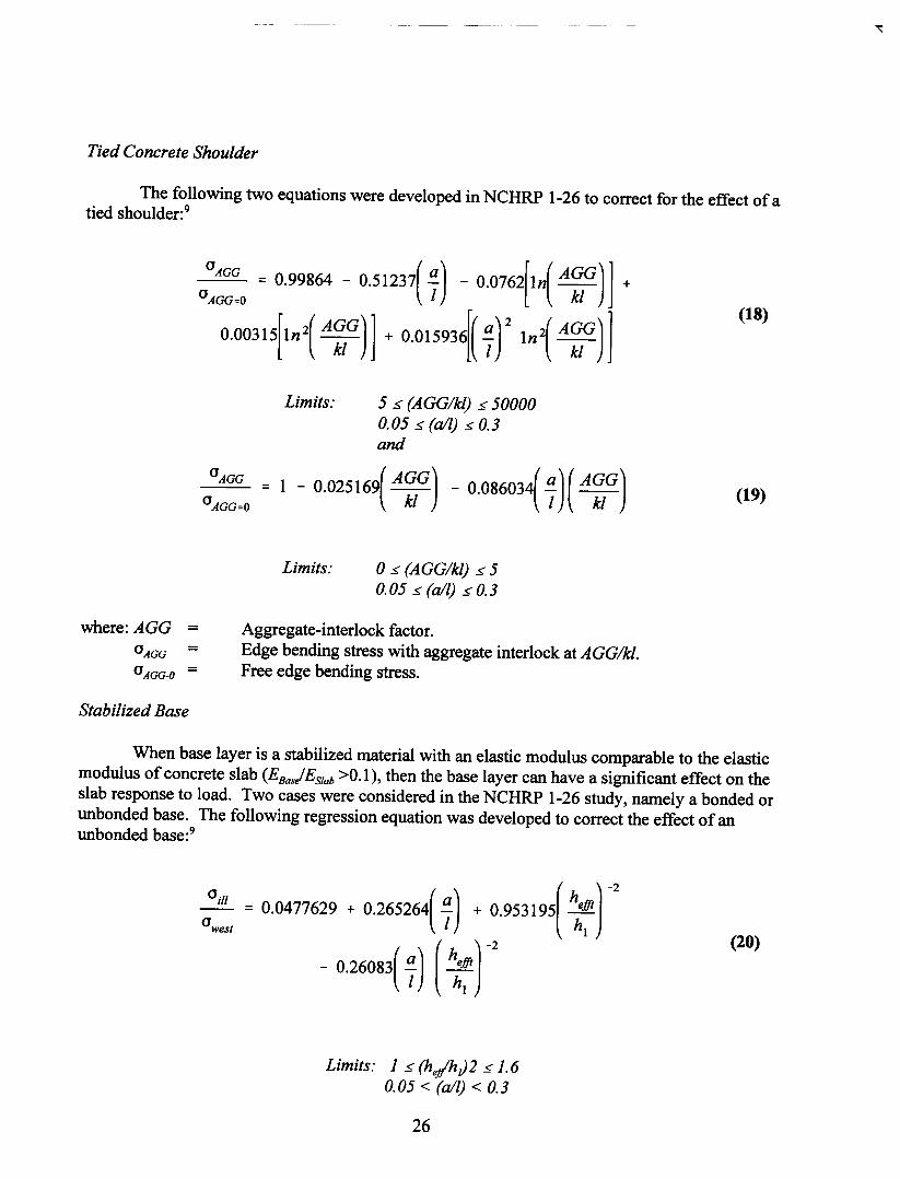
The following two equations were developed in NCHRP 1-26 to correct for the effect of atied shoulder:9

(JAGG = 0.99864 _ 0.SI237( a) _ 0.0762[ln( AGG)] +(JAGG=O I kl

0.00315[ln2( A~) 1 + 0.015936[( ;)' In2

( A~)]5 ~ (AGG/kl) ~ 500000.05 ~ (all) ~ 0.3and

= 1 - 0.02516' A~) _ 0.08603~ ;)( A~G)o ~ (AGG/kl) ~ 50.05 ~ (all) ~ 0.3

Aggregate-interlock factor.Edge bending stress with aggregate interlock at AGG/kl.Free edge bending stress.

When base layer is a stabilized material with an elastic modulus comparable to the elasticmodulus of concrete slab (EBas/ESlab >0.1), then the base layer can have a significant effect on theslab response to load. Two cases were considered in the NCHRP 1-26 study, namely a bonded orunbonded base. The following regression equation was developed to correct the effect of anunbonded base:9

a~:,= 0.0477629 + 0.26526~ ;) + 0.953195( :~ r_ 0.26083( ;) ( hh~)-2

Limits: 1 ~ {he/h)2 ~ 1.60.05 < (all) < 0.3

26

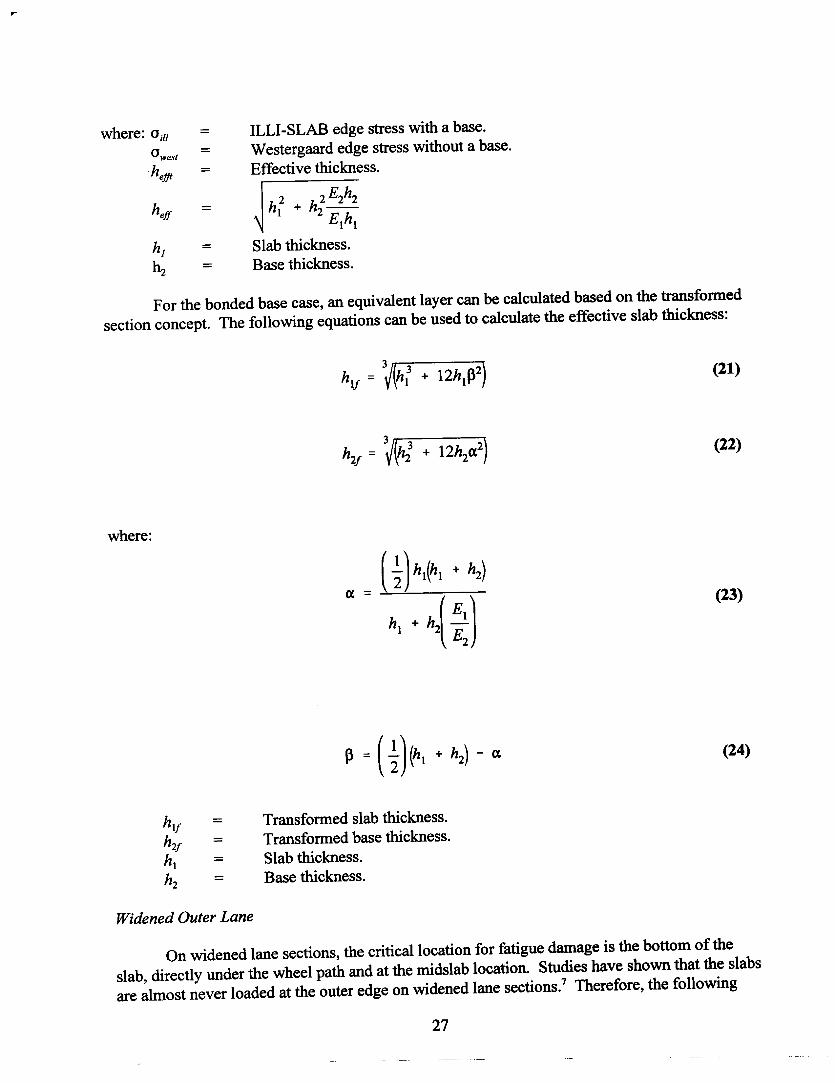
where: oil/ = ILL! -SLAB edge stress with a base.°west = Westergaard edge stress without a base.hefft = Effective thickness.

heff2 2E2h2= hl + hl--

ElhlhI = Slab thickness.h2 = Base thickness.

For the bonded base case, an equivalent layer can be calculated based on the transformedsection concept. The following equations can be used to calculate the effective slab thickness:

(~)hl(hl + 11,)

hI + ~ ::]

hlf =h2f =hI =h2 =

Transformed slab thickness.Transformed base thickness.Slab thickness.Base thickness.

On widened lane sections, the critical location for fatigue damage is the bottom of theslab, directly under the wheel path and at the midslab location. Studies have shown that the slabsare almost never loaded at the outer edge on widened lane sections.7 Therefore, the following

adjustment factor was used to obtain the maximum stress directly under the wheel load for thefew cases of widened lanes:9

= 0.454147 + 0.013211 + 0.386201!!-DN D

_ 0.24565( ~) 2 + 0.053891 ( ~) 3

Adjustment factor for widened lane.1.0 if standard-width lane of3.66 m.Radius of loaded area.Mean wheel location, in from outer edge.Radius of relative stiffness.

The curling stress is determined using the following equation and then combined with theload stress using a regression coefficient in the NCHRP 1-26 procedure:

where: 0c =C =E =aT =LIT =

C E aT !:iT2

Curling stress.Curling stress coefficient.Concrete modulus of elasticity.Concrete coefficient of thermal expansion.Temperature difference between the top and bottom of the slab.

This equation was developed by Westergaard, and Bradbury developed the coefficientsfor solving this equation.1S,16 For maximum stress at the longitudinal edge, the curling stresscoefficient is given by the following equation:

where: L~

C = 1 - 2 COSAcoshA (tanA + tanhA)2 sinA sinhA

Slab length.Radius of relative stiffness.

Warping is the result of non-uniform shrinkage between the top and bottom of the slab.The top of the slab is usually drier than the bottom throughout the year. Therefore, moisturegradient generally tends to cause lifting of the slab corner or warping. The warping is resisted bythe slab weight, causing warping restraint stresses in the slab. The moisture gradients could betreated as equivalent temperature gradients, but insufficient research is available to adequatelyquantify this effect.

During initial construction, as concrete dries it will shrink in volume and thus causeupward warping and warping stresses. The shrinkage normally occurs during concrete's initialcuring phase, and before it has attained its full strength. Since the shrinkage warping stressesoccur early in the concrete aging cycle, and the stresses are long term, some of the warpingstresses may be relieved by concrete creep. Again, there is not enough information to quantifythe effect. Therefore, the warping stresses are not considered in this evaluation. It was assumedthat the warping effects are indirectly accounted for during the calibration/validation of theprocedure.

Combined edge stress.Load stress.Regression coefficient.Curling stress.

where: 0combined

O/ood

R

The regression coefficient R is determined using the following equation:9

R = 1.062 - 0.015757dT - 0.0000876 k - 1.068 L + 0.387317dT LQ Q

+ 1.17x10-11E dTk - 1.81x10-12E dT2k - 1.051X10-9E( ~) 2kdT

+ 1.84xlO-11E dT2~ k - 1.7487( ~) 2dT + 0.000034351dT3

• 86.97( ~) 3_ O.00816396dT' ~

aATx 105•

Concrete coefficient of thermal expansion, E/oF.where: dT

ex

AT =k =L =~ =E =

Temperature difference through the slab, OF.Subgrade modulus of reaction, Ibf/in2/in.Slab length, in.Radius of relative stiffness, in (equation 11).Concrete modulus of elasticity, Ibf/in2•

(Note: Ie/OF = 1.8e/oC, 1°F = 0.56°C, llbf/in2/in = 0.27 MPalm, 1 in = 25.4 mm,1 Ibf/in2 = 6.895 kPa)

The coefficient R is needed because the load and curling stresses are not directly additive.Curling causes various parts of the slab to lift off of the base, invalidating the full contactassumption made in the load stress calculation. The regression coefficient R provides thenecessary adjustment to the curling stress to give the correct combined stress.

Several fatigue models are available to calculate the total number of a specific loadcoverages to failure.3,9 The fatigue model developed in the NCHRP 1-26 study was used in thisproject. The model, which gives the mean number of coverages to failure, defined as 50 percentslabs cracked, is of the following form:

LogN = -1.7136R + 4.284 for R > 1.25LogN = 2.8127R -1.2214 for R < 1.25

Ratio of flexural stress, due to load and climatic factors, to the meanmodulus of rupture of the concrete.Number of coverages to 50 percent slabs cracked.

where: FD =nijk =

Nijk =

i =

FD = L

Total fatigue damage at the critical location in the slab.Number of load repetitions of z-thaxle grouP,J-th load level, and JChtemperature gradient.Number of allowable load repetitions of z-thaxle group,Jib load level, and JChtemperature gradient.A counter for axle group (single dual, tandem dual, and tridem dual).

A counter for axle load magnitude, total of 83 axle load levels in the LTPPdata base for the single, tandem, and tridem axles.A counter for temperature gradient levels, total of 15 levels used.

The number of load repetitions, nijb was computed using traffic data from the LTPPtraffic data base for different axle load group and load magnitude. It was corrected for the trucklateral distribution. Temperature gradient was represented by the frequency of the differenttemperature difference happenings in a typical year, as discussed previously. Therefore, thenumber of load repetitions of a specific axle load group and load level, for a specific temperaturegradient level, can be formulated as follows:

Load repetition count from the LTPP data base for a specific loadgroup and magnitude.Lateral truck distribution factor for loads within 6 in from the edge(8 percent).Frequency of a specific temperature gradient happening in a typicalyear.

A spreadsheet was developed to calculate the allowable number of load repetitions foreach axle load group at each load level for a specific temperature gradient. This was then usedwith the actual load repetition in each group to calculate the total fatigue damage. The calculatedload and curling stresses were compared with the results from the computer program ILLI-CONCdeveloped under the NCHRP 1-26 project to ensure the correctness of the spreadsheet. It isworth noting that, since there were 83 total load levels and 15 temperature gradient levels usedfor the fatigue damage calculation, a total of 1,245 calculations for each LTPP section wasneeded to obtain the cumulative fatigue damage.

At the time of the analysis, a total of 52 JPCP (GPS-3) sections had at least 1 year oftraffic monitoring data. Only these 52 sections were used in the analysis. The specific data usedin the analysis for these 52 sections are given in appendix A. The fatigue analysis results of the52 GPS-3 test sections are shown in figure 6. Also shown in the graph is a transverse crackingmodel recently developed as part of a completed FHWA concrete pavement performance study.17This model is based on field observations from 303 in-service concrete pavements in the UnitedStates and Canada in 1987 and 1992. A total of 465 data points were used to develop the model.The model is listed below:

1001 + 1.41FD 1.66

As shown in figure 6, there were only 15 sections with traffic data in GPS-3 showingsome form of transverse cracking. The sections with fatigue cracking generally follow the trendof the model except for a couple of outliers. There also are many sections with largetheoretically calculated fatigue damage values but with no transverse cracking present, indicatingthat the fatigue damage procedure used and/or the input data used do not fully simulate thefatigue cracking process in JPCP.

This section is concerned with the sensitivity of the fatigue damage calculation as afunction of some key data elements such as traffic counts, modulus of rupture of the concrete,concrete elastic modulus, concrete thermal expansion coefficient, and subgrade modulus ofreaction. A Missouri section, SHRP ID of 5393, was selected to conduct the sensitivity analysis.The following results are all based on the data from this pavement section.

Traffic counts represent the loading conditions of the pavement over time. Theavailability and accuracy of the traffic spectrum data are always a great concern in themechanistic evaluation of the pavement distresses. When Miner's hypothesis is used to calculatethe cumulative fatigue damage as given in equation 20, the total cumulative fatigue damage is thelinear combination of the traffic counts divided by the allowable number of repetitions under thespecific condition. Figure 7 shows the variation of the cumulative fatigue damage when thetraffic counts are all doubled or halved uniformly for all load configuration and load levels.

Modulus of rupture of the concrete is another very important variable in the mechanisticevaluation. Figure 8 gives the sensitivity plot of the fatigue damage with the variation of themodulus of rupture of the concrete. As shown, small changes in Mr will significantly affect thefinal calculated fatigue damage. Similarly, as shown in figure 9, variation in the elastic modulusvalue will have a significant effect on the calculated fatigue damage. The sensitivity plot of thePCC thermal expansion coefficient (figure 10) also shows a significant effect on the calculatedfatigue damage.

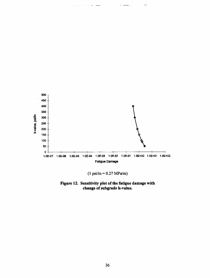
Figures 11 and 12 show the fatigue damage as a function of concrete Poisson's ratio andthe subgrade k-value. As shown, within the range of values commonly used, fatigue damagecomputation is not dependent on either Poisson's ratio or modulus of subgrade reaction used.

Analysis of the LTPP fatigue cracking data indicates that the LTPP data have a highpotential for supporting the development ofM-E procedures for the prediction of fatiguecracking. The analysis presented was limited to showing the potential for use of the LTPP datafor calibrating/validating existing M-E procedures. No specific calibration of the NCHRP 1-26model/procedure for prediction of fatigue cracking was attempted because it was consideredpremature to do so at this time, for the following reasons:

100

90

80

i 70~e! 600fIl,g

50.!!!fIl- 40r::

~ 30Q)ll.

20

10

01.0E-Q7 1.oe-Q6 1.0E-Q5 1.0E-Q4 1.0E-Q3 1.0E-Q2 1.0E-Q1 1.0E+00 1.0E+01 1.0E+02

Fatigue Damage

IfIl,g

.!!!fIl

C

~ 30ll.

100

90

80 AActual data70 ZTrafficl260

XTraffic*250

40

o f-6-X~%-6-~ I Z ~~X-%~ ,1.0E-07 1.0E-06 1.0E-Q5 1.0E-Q4 1.0E-Q3 1.0E-Q2 1.0E-01 1.0E+00 1.0E+01 1.0E+02

Fatigue Damage

800

700

600

500

1 400i300

200

100

o1.OEo07 1.0E-QI 1.0E-QI 1.0E-04 1.0E-G3 1.0E.Q2 1.0E-G1 1.OE.ao 1.OE+01 1.0E+02

F•••• o.m.ge

Fipre 8. Sensitivity plot of the fatigue damage with change of modulus of rupture.

10

9

8

'R 7

c: 6

/,gE 5.&i 4.!!.n 3

2

O+------1f----+---+---+----t---+---+---j------;1.oeo07 1.oe-Q8 1.oe-05 1.0E-04 1.0Eo03 1.OEo02 1.0E.Q1 1.0E+OO 1.OE+01 1.OE+02

Flltigue OarN1g8

Figure 9. Sensitivity plot of the fatigue damage with change of elasticmodulus of the slab.

0.5

0.45

0.4

0.35

t 0.3

i 0.250.2ID.

0.15

0.1

0.05

O+----+----f-----I---+---+----+----+----+-----j1.0E-Q7 1.0E-Q6 1.0E-05 1.0E-04 1.0E-Q3 1.0E-Q2 1.0E-Q1 1.0E+OO 1.0E+01 1.0E+02

Fatigue Damage

Figure 10. Sensitivity plot of the fatigue damage with change of thePCC thermal expansion coefficient.

/O+----1I-----+----+-__ +-_--+~ _ __+_-~+_--+__-__11.0E-07 1.0E-Q6 1.0E-Q5 1.0E-Q4 1.0E-Q3 1.0E-Q2 1.0E-Q1 1.0E+OO 1.0E+01 1.0E+02

Fatigue Damage

Figure 11. Sensitivity plot ofthe fatigue damage with change ofPoisson's ratio of the slab.

450

400

350

300

250

200

150

100

50

o1.0E-Q7 1.0E-Q6 1.0E-Q5 1.0E-Q4 1.0E-Q3 1.0E-Q2 1.0E-01 1.0E+OO 1.0E+01 1.0E+02

Fatigue Damage

Figure 12. Sensitivity plot of the fatigue damage withchange of subgrade k-value.

2. Concern with the quality of the extrapolated traffic data. Even though weigh-in-motion data are beginning to be available for many GPS test sections, thesampling precision, the reliability of the axle load measurements, lateraldistribution of traffic, and the backcasting of traffic need further clarity.

3. Concern with the fatigue cracking distress data. The fatigue data need to be re-evaluated to ensure that random cracking data are omitted from the fatiguecracking data.

5. A better characterization needs to be developed to incorporate curling andwarping effects. The availability of site specific coefficient of thermal expansionfor the concrete would greatly aid in this effort.

In summary, it is concluded that the NCHRP 1-26 approach for predicting fatiguecracking (in terms of pertinent slabs cracked) appears to be reasonable, given the manyunknowns that continue to hinder a complete development of the prediction methodology. Asthe LTPP data base is progressively improved upon, both in terms of quality and in terms of datacoverage, it is expected that the NCHRP 1-26 approach will be improved and that a more reliableand better calibrated fatigue cracking prediction procedure will be developed.

Transverse joint faulting is the difference in elevation of two adjacent slabs at a joint.Typically, the leave slab is at a lower elevation than the approach slab. Many jointed PCCpavements experience serious faulting with time. A faulting level in excess of 6 mm isconsidered unacceptable for high-volume highways. Faulting is significantly affected by thepresence of dowel bars and permeable/non-erodible base, joint spacing, and subdrainageconditions.

Over the years, many studies have been conducted to research the development offaulting. Various models have been developed to predict faulting. Typically, these models havebeen empirical in form and incorporate the use of the equivalent single-axle load parameter torepresent the traffic loading. The only mechanistic-based faulting prediction procedures arethose developed under the sponsorship of the Portland Cement Association (PCA). Thesemechanistic-based models were the ones used in the analysis of the LTPP faulting data, asreported here.

Prior to 1984, mechanistic thickness design procedures for concrete pavements werebased on the principle of limiting the flexural stresses in a slab to avoid flexural fatigue cracksdue to load repetitions. Erosion criteria were incorporated into the 1984 PCA design proceduresince some modes of pavement distress, such as pumping, faulting, and shoulder distress, areunrelated to fatigue. Distress due to erosion is considered to be more closely related to slabdeflections than to flexural stresses. At slab comers and edges in the presence of water and manyrepetitions of heavy axle loads, pumping (erosion of subgrade, subbase, and shoulder materials),voids under and adjacent to the slab, and faulting of pavement joints (especially in pavements atnondoweledjoints) can occur. Voids or the loss of uniform support increase slab stresses andstrains and can lead to premature cracking.

Attempts to correlate comer deflections to AASHO Road Test performance data, whereall pavement sections were doweled, and to faulting studies were not successful. 18 The principalmode of failure at the AASHO Road Test was pumping of the granular subbase from under theslabs. It was found that, to be able to predict the AASHO Road Test performance, differentvalues of deflection criteria would have to be applied to different slab thicknesses, and to asmaller extent, different slab support values.

Better performance prediction was obtained by correlation of the subbase pressuremultiplied by the slab comer deflection. Subbase pressure at the slab-foundation interface iscomputed as the modulus of subgrade reaction, k, multiplied by the slab deflection. Power, orrate of work, with which an axle load deflects the slab is the parameter used for the erosioncriterion. For a unit area, the power term incorporates the product of pressure and deflection

divided by a measure of the length of the deflection basin (radius of relative stiffness, I). Theconcept is that a thinner pavement with its shorter deflection basin receives a faster punch than athicker slab. At equal products of deflection and pressure, the thinner slab is subjected to a fasterrate of work or power.

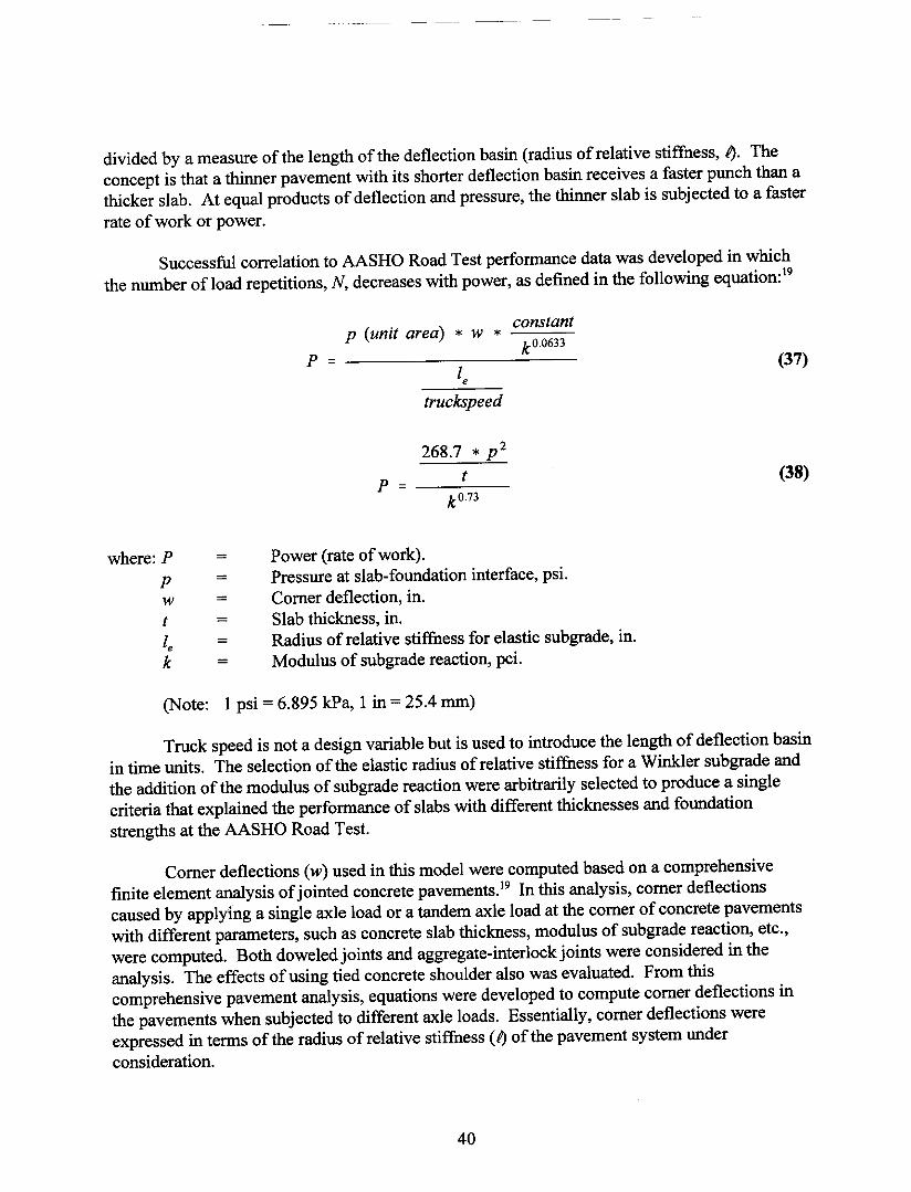
Successful correlation to AASHO Road Test performance data was developed in whichthe number ofload repetitions, N, decreases with power, as defined in the following equation:19

constantkO.0633

p = ---------Ie

truckspeed

268.7 * p2t

kO.73

where: P =

P =

w =

t =

Ie =k =

Power (rate of work).Pressure at slab-foundation interface, psi.Comer deflection, in.Slab thickness, in.Radius of relative stiffness for elastic subgrade, in.Modulus of subgrade reaction, pci.

Truck speed is not a design variable but is used to introduce the length of deflection basinin time units. The selection of the elastic radius of relative stiffness for a Winkler subgrade andthe addition of the modulus of subgrade reaction were arbitrarily selected to produce a singlecriteria that explained the performance of slabs with different thicknesses and foundationstrengths at the AASHO Road Test.

Comer deflections (w) used in this model were computed based on a comprehensivefinite element analysis of jointed concrete pavements.19 In this analysis, comer deflectionscaused by applying a single axle load or a tandem axle load at the comer of concrete pavementswith different parameters, such as concrete slab thickness, modulus of subgrade reaction, etc.,were computed. Both doweled joints and aggregate-interlock joints were considered in theanalysis. The effects of using tied concrete shoulder also was evaluated. From thiscomprehensive pavement analysis, equations were developed to compute comer deflections inthe pavements when subjected to different axle loads. Essentially, comer deflections wereexpressed in terms of the radius of relative stiffness (I) of the pavement system underconsideration.

The development of the 1984 design erosion criteria was also generally related to studieson joint faulting. These studies included pavements in Wisconsin, Minnesota, North Dakota,Georgia, and California, and included a range of variables not found at the AASHO Road Test.Additional variables such as increased amounts of truck traffic, non-doweled pavements, a widerrange of pavement service life, and stabilized subbases were included in the erosion criteriaverification.

The analysis of data from the AASHO Road Test and available faulting studies resultedin the following erosion prediction equation:

log Nj = 14.524 - 6.777 * (C1 * Pj - 9.0)°·103

Allowable load repetitions to end of design period for axle-group i.Power term for axle-group i.1 - ( k / 2000 * 4/ t) 2.

The constant C] is an adjustment factor that has a value close to 1.0 for normal granularsubbases and decreases to approximately 0.90 for high-strength subbases.

EROSION, % = 100 * :En; * ( ~]

Accumulated erosion, percent.Expected number of axle-load repetitions for axle-group i.Allowable number of repetitions for axle-group i.0.06 for pavements without a shoulder and 0.94 for pavements with atied concrete shoulder.

Truck wheel loads placed at the outside pavement edge create more severe deflectionconditions than any other load position. As the truck placement moves inward a few millimetersfrom the edge, the effects decrease substantially. Only a small fraction of all the trucks run withtheir wheels placed at the edge. Studies on pavement edge encroachment show that most trucksare driven with the outside wheels placed about 0.6 m from the edge.6,7 For the design procedurethe most severe condition noted in encroachment studies of 6 percent of trucks at pavement edgeswas assumed. This added an additional factor of safety and accounted for recent changes in theUnited States permitting wider trailers. At increasing distances inward from the pavement edge,the frequency of load applications increases while the magnitude of stress and deflectiondecreases.

Where there is no tied concrete shoulder, comer loadings are critical. When a concreteshoulder is used, the greater number of loadings inward from the pavement comer are critical.

Most conventional analyses of concrete pavement systems assume that subbase-subgradelayers do not exist beyond the pavement edge. The MATS finite element computer program wasused to investigate the effect and contribution of subbase-subgrade support away from thepavement edge.20 For different moduli of subgrade reaction and slab thicknesses, the free comerdeflections were equal to or less than 89.6 percent of those conditions without the outsidesubgrade-subbase support. The 10.4 percent comer deflection reduction factor was incorporatedinto the PCA erosion design charts for pavements without a tied concrete shoulder. For slabswith a concrete shoulder, the subgrade support outside the shoulder edge is too far from the trucktraffic to have any beneficial effect on reducing deflections.

During 1992, data from existing performance data bases were used to develop faultingprediction models to include the PCA erosion criteria as a parameter. Transverse joint data werecollected from existing State Department of Transportation (DOT) pavement management databases and pavement performance research data bases.21.22.23Joint faulting measurements obtainedby the Construction Technology Laboratories also were added to the PCA data base.

The collection of faulting and traffic data used in the analysis is summarized by regionand State in table 6. Survey data were collected in dry-freeze, dry non-freeze, wet-freeze, andwet non-freeze sections of the United States. Joint faulting data from a total of 509 projects werecollected. Region classification criteria for wet or dry and non-freezing or freezing aresummarized in table 7.24

The accumulated percent erosion was correlated with degree of faulting for eachpavement section. Modulus of subgrade reaction (k-value) and increases in support due togranular and stabilized subbases were calculated using the PCA thickness design guidelineprocedures.2s Truck load distribution and frequency were selected for each project from W-4load tables. One-way average daily traffic (ADT) was used to estimate the proportion of trucksin the right lane. Erosion for several load categories was accumulated from the truckproportions, load frequency, and average daily truck traffic (ADTT).

Important environmental factors included in the analysis were the levels of moisture andtemperature range. Levels of moisture were categorized by the freezing index (degree-daysbelow O°C), average annual precipitation, soil drainability (AASHTO soil type), and presence oflongitudinal edge drains. Some previous research work has indicated that joint opening wasstatistically significant in predicting faulting only at non-doweled pavement joints. The degree ofjoint opening affecting joint load transfer and potential for faulting is a function of annualtemperature range (maximum daily temperature minus minimum temperature), slab length(broadly categorized into jointed reinforced, JRCP, and jointed plain concrete pavement, JPCP),concrete coefficient of thermal expansion, and concrete drying shrinkage.

A statistical analysis computer program was used to develop the relationships betweenaccumulated erosion and joint faulting. Non-linear regression analysis techniques were used indevelopment of the faulting prediction model. An initial set of power parameters and variable

Climatic No. of No. of DataState Reldon Projects Points Data Source

Arizona Dry Non-Freeze 7 7 ref. 22California Dry and Wet Non-Freeze 85 814 DOT, refs.21 & 22

Connecticut Wet-Freeze 7 9 DOTFlorida Wet Non-Freeze 50 283 DOT, refs. 22 & 23Georgia Wet Non-Freeze 28 65 ref. 21

Iowa Dry and Wet Freeze 38 38 DOTIllinois Wet-Freeze, Wet Non-Freeze 8 15 DOT

Louisiana Wet Non-Freeze 28 297 ref. 21Michigan Wet-Freeze 12 12 ref. 22Minnesota Dry-Freeze 105 921 DOT, refs.21 & 22

North Carolina Wet Non-Freeze 13 63 DOT, ref. 22New York Wet-Freeze 21 21 refs. 22 & 23

Ohio Wet-Freeze 59 59 refs. 22 & 23Pennsylvania Wet-Freeze 5 5 ref. 22

Utah Dry-Freeze 33 231 ref. 21Wisconsin Dry and Wet Freeze 10 10 DOT

Total 509 2850

Annual Rainfall, Freezing Index,Climatic Zone in. F De2ree-Days

Wet Non-Freeze Greater than 28 Less than 100Wet-Freeze Greater than 28 Greater than 100

Dry Non-Freeze Less than 28 Less than 100Dry-Freeze Less than 28 Greater than 100

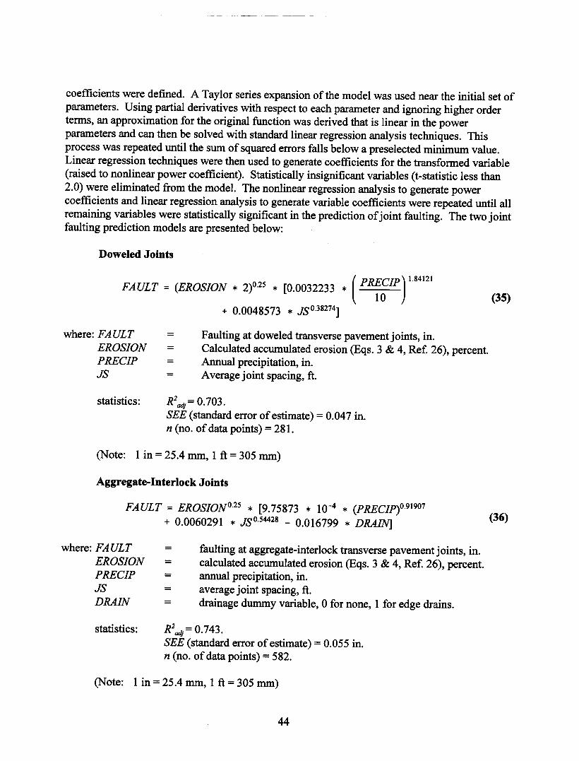
coefficients were defined. A Taylor series expansion of the model was used near the initial set ofparameters. Using partial derivatives with respect to each parameter and ignoring higher orderterms, an approximation for the original function was derived that is linear in the powerparameters and can then be solved with standard linear regression analysis techniques. Thisprocess was repeated until the sum of squared errors falls below a preselected minimum value.Linear regression techniques were then used to generate coefficients for the transformed variable(raised to nonlinear power coefficient). Statistically insignificant variables (t-statistic less than2.0) were eliminated from the model. The nonlinear regression analysis to generate powercoefficients and linear regression analysis to generate variable coefficients were repeated until allremaining variables were statistically significant in the prediction of joint faulting. The two jointfaulting prediction models are presented below:

FAULT = (EROSION * 2)'·25 * [0.0032233 * ( P~~IP) 1.8412I

+ 0.0048573 * JSO.38274]

where: FAULTEROSIONPRECIPJS

Faulting at doweled transverse pavement joints, in.Calculated accumulated erosion (Eqs. 3 & 4, Ref. 26), percent.Annual precipitation, in.Average joint spacing, ft.

R2adj= 0.703.

SEE (standard error of estimate) = 0.047 in.n (no. of data points) = 281.

FAULT = EROSIONo.25 * [9.75873 * 10-4 * (PRECIP)O.91907+ 0.0060291 * JSO.54428 - 0.016799 * DRAIN]

where: FAULTEROSIONPRECIPJSDRAIN

faulting at aggregate-interlock transverse pavement joints, in.calculated accumulated erosion (Eqs. 3 & 4, Ref. 26), percent.annual precipitation, in.average joint spacing, ft.drainage dummy variable, 0 for none, 1 for edge drains.

R2adj= 0.743.

SEE (standard error of estimate) = 0.055 in.n (no. of data points) = 582.

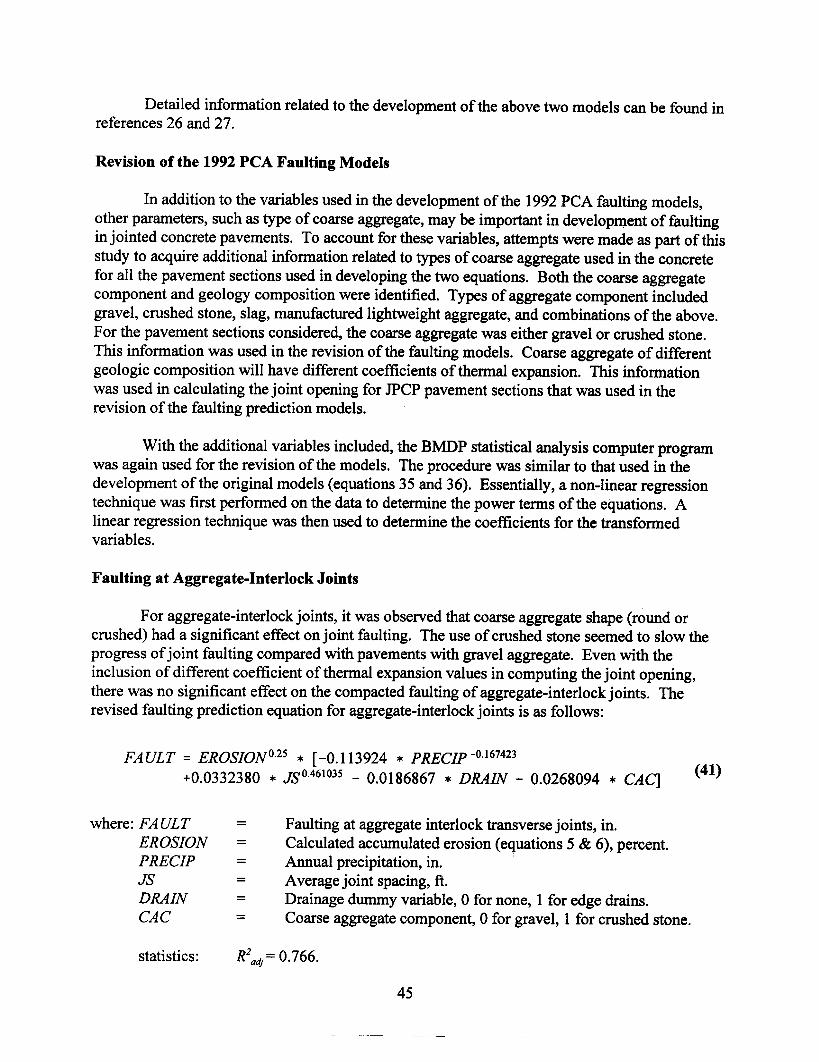
Detailed information related to the development of the above two models can be found inreferences 26 and 27.

In addition to the variables used in the development of the 1992 PCA faulting models,other parameters, such as type of coarse aggregate, may be important in development of faultingin jointed concrete pavements. To account for these variables, attempts were made as part of thisstudy to acquire additional information related to types of coarse aggregate used in the concretefor all the pavement sections used in developing the two equations. Both the coarse aggregatecomponent and geology composition were identified. Types of aggregate component includedgravel, crushed stone, slag, manufactured lightweight aggregate, and combinations of the above.For the pavement sections considered, the coarse aggregate was either gravel or crushed stone.This information was used in the revision of the faulting models. Coarse aggregate of differentgeologic composition will have different coefficients of thermal expansion. This informationwas used in calculating the joint opening for JPCP pavement sections that was used in therevision of the faulting prediction models.

With the additional variables included, the BMDP statistical analysis computer programwas again used for the revision of the models. The procedure was similar to that used in thedevelopment of the original models (equations 35 and 36). Essentially, a non-linear regressiontechnique was first performed on the data to determine the power terms of the equations. Alinear regression technique was then used to determine the coefficients for the transformedvariables.

For aggregate-interlock joints, it was observed that coarse aggregate shape (round orcrushed) had a significant effect on joint faulting. The use of crushed stone seemed to slow theprogress of joint faulting compared with pavements with gravel aggregate. Even with theinclusion of different coefficient of thermal expansion values in computing the joint opening,there was no significant effect on the compacted faulting of aggregate-interlock joints. Therevised faulting prediction equation for aggregate-interlock joints is as follows:

FAULT = EROSIONo.2s * [-0.113924 * PRECIP -0.167423+0.0332380 * JSO.46103S- 0.0186867 * DRAIN - 0.0268094 * CAe]

where: FAULTEROSIONPRECIPJSDRAINCAC

Faulting at aggregate interlock transverse joints, in.Calculated accumulated erosion (equations 5 & 6), percent.Annual precipitation, in. 'Average joint spacing, ft.Drainage dummy variable, 0 for none, 1 for edge drains.Coarse aggregate component, 0 for gravel, 1 for crushed stone.

SEE (standard error of estimate) = 0.048 in.n (no. of data points) = 683.

Compared with the original 1992 peA faulting prediction equation for aggregate-interlock joints, the revised equation shows some improvement in terms of both the adjustedcoefficient of determination (R2

adj) and the standard error of estimate (SEE). The revisedprediction equation should therefore provide better estimation of joint faulting. As presented infigure 13, an approximately normal distribution centered around zero is observed for theprediction error.

For aggregate-interlock joints, a sensitivity analysis indicates that faulting increases withan increase in the value of the variable in question. Results of the sensitivity analysis for non-doweled joints are shown in table 8.

Inde endent VariableIncrease in erosion

Increase in reci itationIncrease in .oint s acin

Use of crushed coarsea re ate

Use of ed e drains

Effect on FaultinIncreaseIncreaseIncreaseIncrease

Sensitivivaries with erosion

mediumhih

medium

Plots of faulting versus accumulated erosion for aggregate-interlock joints are shown infigures 14 through 17 for pavements using different coarse aggregate (crushed stone or gravel)and for pavements in wet regions (annual precipitation of 1016 mm) and in dry regions (annualprecipitation of 508 mm).

The annual precipitation has a significant effect on joint faulting. For example, at 100percent erosion for a 4.6-m-Iong slab in a region with an annual precipitation of 1016 mm thepredicted j oint faulting for a pavement using gravel coarse aggregate, as shown in figure 16, is4.4 mm. For the same conditions but with a lower precipitation of 508 mm, the aggregateinterlock model shown in figure 14 predicts faulting of 3.8 mm when no edge drains are present.A 50 percent reduction in precipitation results in a 14 percent reduction in faulting.

Joint spacing also has a significant effect on predicted aggregate-interlock joint faulting.For example, at 100 percent erosion for a 12.2-m-Iong slab in a region with an annualprecipitation of 508 mm the predicted faulting fQr a pavement with gravel coarse aggregate, asshown in figure 14, is 9.1 mm when edge drains are not used. For the same conditions but with asmaller joint spacing of 4.6 m the aggregate-interlock joint model, as shown in figure 14, predictsfaulting of 3.8 mm. A 63 percent reduction in joint spacing results in a 58 percent reduction infaulting.

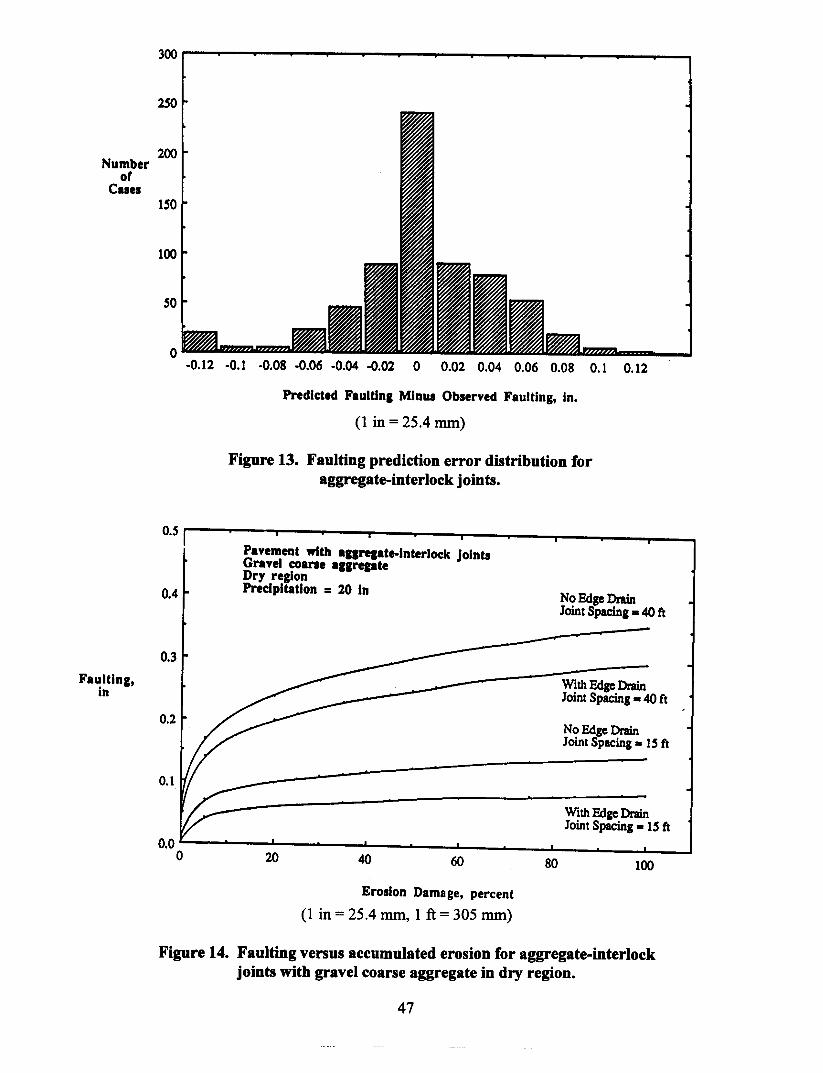
200Number

orCases

ISO

100

SO

Predicted Faultlna Minus Observed Faulting, In.

(1 in = 25.4 mm)

Figure 13. Faulting prediction error distribution foraggregate-interlock joints.

Pavement with -a,rea_te-Interlock JointsGravel coane aaarea_teDry regionPrecipitation = 20 In No Edge Drain

Joint Spacing. 40 ft

With Edge DrainJoint Spacing. 40 ft

Faulting,in

No Edge DrainJoint Spacing. IS ft

With Edge DrainJoint Spacing. IS ft

0.0o

Erosion Damage, percent

(l in = 25.4 mm, 1 ft = 305 mm)

Figure 14. Faulting versus accumulated erosion for aggregate-interlockjoints with gravel coarse aggregate in dry region.

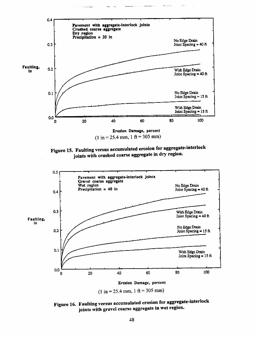
Faulting,in

Faulting,in

Pavement with aggregate-interlock jointsCrushed coarse agaregateDry regionPrecipitation = 20 in

0.0oErosion Damage, percent

(1 in = 25.4 mm, 1 ft = 305 mm)

No Edge DrainJoint Spacing = 40 ft

With Edge DrainJoint Spacing = 40 ft

No Edge DrainJoint Spacing = 15 ft

With Edge DrainJoint Spacing = 15 ft

80 100

Figure 15. Faulting versus accumulated erosion for aggregate-interlockjoints with crushed coarse aggregate in dry region.

Pavement with aggregate-interlock jointsGr •••.el coarse aggregateWet regionPrecipitation = 40 in

0.0 o

No Edge DrainJoint Spacing. 40 ft

With Edge DrainJoint Spacing. 40 ft

No Edge DrainJoint Spacing • 15 ft

With Edge DrainJoint Spacing = 15 ft

Figure 16. Faulting versus accumulated erosion for aggregate-interlockjoints with gravel coarse aggregate in wet region.

Faulting,in

Pavement with aggregate-interlock jointsCrushed coarse aggregateWet regionPrecipitation = 40 in

0.0 o

No Edge DrainJoint Spacing = 40 ft

With Edge DrainJoint Spacing = 40 ft

No Edge DrainJoint Spacing = 15 ft

With Edge DrainJoint Spacing = 15 ft

Figure 17. Faulting venus accumulated erosion for aggregate-interlockjoints with crushed coane aggregate in wet region.

Also shown in these figures, the use of longitudinal edge drains and the use of crushedstone coarse aggregate were statistically significant in reducing aggregate interlock joint faulting.However, the effectiveness of these two parameters in reducing aggregate-interlock faulting isdependent on the percent erosion level. They become more effective as percent erosionincreases.

For pavements with doweled joints, statistical analysis showed that the coarse aggregatetype (crushed stone or gravel) had significant effects on the predicted joint faulting. However,when compared with the 1992 PCA faulting prediction equation, the new prediction equation,with the inclusion of coarse aggregate type as a predictor, had lower R2 adj (0.648) and higher SEE(0.072). It was therefore determined that the coarse aggregate type need not be included as apredictor in estimating faulting for doweled joints. Instead, the 1992 PCA faulting predictionequation (equation 35) was selected for use in this study. The equation is given below:

FAULT ~ (EROSION *2)0.2' * 0.0032233 * ( P~~IP) L84121

+ 0.0048573 * JSO.38274

where: FAULTEROSIONPRECIPJS

Faulting at doweled transverse pavement joints, in.Calculated accumulated erosion (equations 5 and 6), percent.Annual precipitation, in.Average joint spacing, ft.

R2adj= 0.703.

SEE (standard error of estimate) = 0.047 in.n (no. of data points) = 281.

The predicted faulting error distribution is shown in figure 18. Again, the predictionerrors are symmetrically distributed around zero.

Similar to the aggregate-interlock joints, a sensitivity analysis indicates that faultingincreases with an increase in the value of the variable in question. Results of the sensitivityanalysis for doweled joints are shown in table 9.

Effect on FaultinIncreaseIncreaseincrease

Sensitivivaries with erosion

hihmedium

Plots of faulting versus accumulated erosion are shown in figures 19 and 20 for wetregions (annual precipitation of 1016 rnm) and dry regions (annual precipitation of 508 rnm),respectively. Figures 14 through 17, 19 and 20 should not directly be used for comparing theeffectiveness of dowel bars in reducing faulting since they are plotted as a function of erosion.Erosion is computed using erosion factors that include the benefits (higher amount of allowableloads) of dowel bars.

Again, the annual precipitation has a significant effect on joint faulting for doweledjoints. For example, at 100 percent erosion for a 4.6-m-long slab in a region with an annualprecipitation of 1016 rnm the predicted faulting as shown in figure 19, is 5.3 rnm. For the sameconditions but with a lower precipitation of 508 rnm the doweled model shown in figure 20predicts faulting of 2.4 rnm. A 50 percent reduction in precipitation results in a 50 percentreduction in faulting.

Joint spacing also has a significant effect on predicted faulting. For example, at 100percent erosion for a 12.2-m-long slab in a region with an annual precipitation of 508 rnm thepredicted faulting for doweled joints, as shown in figure 20, is 3.0 rnm. For the same conditionsbut with a smaller joint spacing of 4.6 m the doweled joint model shown in figure 20 predictsfaulting of 2.4 rnm. A 63 percent reduction in joint spacing results in a 19 percent reduction infaulting.

Evaluation of the Revised 1992 peA Faulting Models Using SHRP LTPP Data (GPS-3 andGPS-4)

Data obtained from the LTPP data base for GPS-3 (JPCP) and GPS-4 (JRCP) testsections were used in evaluating the revised faulting models. Types of information required fromthe LTPP data base included the following:

• Pavement structural design parametersPCC thicknessPCC modulus of elasticityModulus of sub grade reactionCoarse aggregate typesType and thickness of base or subbase layersType of pavement shoulderJoint type, doweled or aggregate-interlockAverage joint spacing

• Traffic informationAxle load distribution

Annual precipitationFreezing index

NumberorCases

Faulting,in 0.15

0.00 o

Predicted Faulting Minus Observed Faulting, in(1 in = 25.4 mm)

Figure 18. Faulting prediction error distribution for doweled joints.

Pavement with doweled jointsWet regionPrecipitation = 40 in

Figure 19. Faulting versus accumulated erosion for doweled joints in wet region.

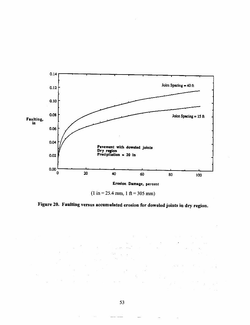
Faulting,in

Pavement with doweled jointsDry regionPrecipitation = 10 in

0.00 o

Most of the data were extracted from the data base (as discussed in chapter 2) and directlyused in the analysis. However, some manipulation was required for some of the data before theycould be used in the evaluation process.

Attempts were first made to use the measured concrete modulus of elasticity data in theevaluation. However, too many missing data made this approach impossible. As the secondstep, PCC moduli of elasticity backcalculated from falling weight deflectometer (FWD) test datawere considered. However, a closer examination of the backcalculated concrete modulus valuesrevealed that most of the values were much too high, with some reaching 90,000 MPa. Sincethe computed erosion factor caused by traffic loads on pavement systems will be affected by theconcrete modulus of elasticity, the use of unrealistically high values was considered inadequate.

For the purpose of this analysis, the best possible material testing data available at thetime of analysis appeared to be the 28-day compressive strength of concrete specimens. For mostof the test sections evaluated in this study, the 28-day compressive strength data were used toestimate concrete modulus of elasticity. For a few cases, the 28-day compressive strength datawere not available and the concrete modulus of rupture (flexural strength) data were used toestimate the modulus of elasticity values for that section.

The modulus of subgrade reaction values backcalculated from FWD deflection tests wereavailable for all the pavement sections considered in this analysis. For pavements with astabilized or granular base or subbase layer, their backcalculated k-values were adjusted toaccount for the increased support provided by the presence of base and/or subbase layers usingthe PCA thickness design guideline procedures.29

To compute the accumulated erosion of a pavement system, the axle load distributionover its service life for all the weight categories is required. Unfortunately, very limited trafficdata were available. The lack of axle load distribution data reduced the number of test sectionsthat could be evaluated. A total of 57 pavement sections were included in this study, consistingof20 pavements with aggregate-intedockjoints and 37 with doweled joints. Furthermore, thedata available were mostly for a single year only. To estimate the total amount of traffic traveledon a pavement during its entire service life, an annual traffic increase rate of 2 percent wasassumed in the analysis (as discussed in chapter 2). This assumption somewhat overestimatesthe joint faulting. The effect of annual traffic growth rate on the predicted joint faulting ispresented in a latter section.

With all the information obtained and derived from the LTPP data base, the predictedfaulting for aggregate-interlock joints was computed using the revised 1992 joint faultingequation. As mentioned earlier, complete information was obtained for 20 pavement sections.The differences between the predicted and observed faulting (prediction errors) ranged from -1.5mm to 1.32 mm, with a mean value of -0.76 mm and a standard deviation of 0.79 mm. Aspresented in figure 21, the prediction errors are distributed approximately symmetrically aroundzero, indicating reasonable predicting power of the faulting model.

A paired-t test also was performed to further evaluate the adequacy of the predictionequation. It was concluded that, at the 95 percent confidence level, the null hypothesis of nodifference between the predicted and observed faulting could not be rejected. In fact, the nullhypothesis could not be rejected even at the 70 percent confidence level. This conclusionsuggested that the developed faulting prediction model is reasonable for predicting faulting foraggregate-interlock joints. The comparison of the predicted and the observed faulting foraggregate-interlock joints is shown in figure 22. In the figure, the solid line represents the line ofequality and the two dashed lines are one standard deviation away from the line of equality. It isobserved that most of the data points fall within ±1 standard deviation from the line of equality.

Joint faulting was computed using the 1992 joint faulting equation and data obtainedfrom the LTPP data base for doweled joints. A total of37 pavement sections having the neededdata were evaluated. The differences between the predicted and observed faulting (predictionerrors) ranged from -1.7 mm to 3.0 mm, with a mean value of 0.56 mm and a standard deviationof 1.24 mm. Plotted in figure 23, the prediction error distribution for doweled joints showsskewness toward the positive side, indicating an overestimate of the predicted faulting. A paired-t test further revealed that the null hypothesis of no difference between the predicted andobserved faulting was rejected at the 95 percent confidence level. It can therefore be inferred thatthere is a difference between the predicted and observed faulting.

The predicted faulting is plotted against the observed faulting in figure 24. It is observedthat most of the measured faulting values are in the range between 0.00 and 1.27 mm. The use ofdoweled joints seemed to significantly reduce joint faulting. It is also clear that, at this lowerrange, the prediction equation tends to overestimate joint faulting for doweled joints. Formeasured faulting greater than 1.27 mm, the equation seems to provide better faulting estimatesfor doweled joints.

As presented in the previous sections, the aggregate-interlock model provided reasonablygood estimates for j oint faulting for the 20 LTPP sections evaluated. Statistically, no differencecould be claimed between the predicted and observed faulting for aggregate-interlock joints.However, an overestimate of the faulting was evident for doweled joints, as indicated by thepositive skewness of the faulting prediction error distribution shown in figure 23.

6

S

4Numberor

Cues3

0.00U.OO

••

a. standard deviationor prediction errors• 0.031 In

Measured 'aultlna, In

(1 in = 25.4 mm)

Figure 22. Predicted faulting versus measured faulting foraggregate-interlock joints.

Numberor 6Cues

Predicted Faultlnl Minus Observed Faulting

(l in = 25.4 mm)

a = standard deviationor prediction errors= 0.049 In

Measured Faulting, In

(l in = 25.4 mm)

The PCA faulting prediction equation utilizes the concept of erosion damage of thepavements caused by traffic loads. Erosion damage is determined based on traffic load-inducedcomer deflections in the pavements. Among other parameters, concrete modulus of elasticity isimportant in determining the comer deflections. However, site specific data were not available atthe time of analysis. In this study, concrete modulus of elasticity was estimated from its 28-daycompressive strength. It is believed that use of actual measured concrete modulus of elasticitydata will increase the prediction accuracy.

Similar to other mechanistic-based procedures, the joint faulting prediction equationsrequire the use of traffic axle load distribution in the analysis. Converted traffic indices, such as80-kN ESAL currently used in the AASHTO design procedure, cannot be used. At the time ofanalysis, the LTPP data base contained traffic axle load distribution data for a very limitednumber of pavement sections. Furthermore, for these limited number of test sections, axle loaddistribution data were only available for a particular year, and the cumulative amount of trafficvolume on the pavements had to be estimated using a 2 percent annual traffic growth rate, asdiscussed in chapter 2. This assumption was believed to be conservative and might havecontributed to the overestimate of the doweled joint faulting. Reliable traffic data (in terms ofaxle loadings) are essential for any pavement evaluation using the LTPP data base.

Sensitivity analyses of annual traffic growth rate on computed faulting were performedfor both doweled and aggregate-interlock joints, and are presented in figure 25. It can beobserved that traffic growth rate only slightly affects the predicted faulting for both types ofjoints. As the annual traffic growth rate increases from 2 to 15 percent, the computed faultingdecreases from 1.32 mm to 1.14 mm and from 1.60 mm to 1.50 mm for the aggregate-interlockjoint and the doweled joint, respectively. It should be noted that because traffic is backcastedfrom a current year, higher growth rates result in lower cumulative traffic loadings. Theprediction errors may be reduced slightly if annual growth rate of traffic can be estimatedreliably.

The lack of required material testing and traffic data reduced the number of LTPP testsections that could be evaluated. However, the quality of the faulting data may be a more seriousdeficiency of the data base. For instance, faulting observed at two consecutive years at manysections had a difference in excess of 2.54 mm. In some cases, faulting measured at the wheelpath was very different from that measured at the comer. These inconsistencies make the use ofthe LTPP data difficult. The following are a few examples of inconsistencies of the faulting data:

• Pavement section 1-3028Faulting at wheel path: 0.000 mmFaulting at comer: 3.28 mm

• Pavement section 12-4138Faulting at wheel path: 0.000 mmFaulting at comer: 5.13 mm

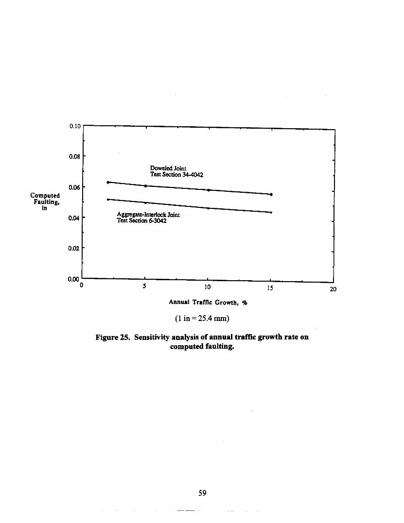
0.08Doweled JointTest Section 34-4042

••0.06 • •

Computed •Fa'!lting,

..an

Aggregate-Interlock 10int •0.04 Test Section 6-3042

0.00 o

Figure 25. Sensitivity analysis of annual traffic growth rate oncomputed faulting.

• Pavement section 1-4084Faulting measured in 1991 (21 years): 4.29 mmFaulting measured in 1993 (23 years): 8.79 mm

• Pavement section 34-4042Faulting measured in 1991 (24 years): 4.70 mmFaulting measured in 1992 (25 years): 5.56 mmFaulting measured in 1993 (26 years): 3.58 mm

In general, the LTPP data base provides valuable information that can be used to develop,calibrate, and/or validate mechanistic-based pavement analysis and design procedures. However,the issues of lack of material testing and traffic data, and the quality of the performance data needto be addressed.

The two faulting prediction models, one for aggregate-interlock joints and the other fordoweled joints, developed in 1992 were revised in an attempt to include coarse aggregated typeas a predictor. Reasonable coefficients of determination (greater than 0.70) were obtained. Fordoweled joints, important factors that will influence faulting include erosion, precipitation, andjoint spacing. For aggregate-interlock joints, erosion, precipitation, joint spacing, the use of edgedrains, and coarse aggregate types were found to be significant in affecting joint faulting.

Sensitivity analyses of the two joint faulting prediction equations have revealed thatfaulting will increase with increased erosion, precipitation, or joint spacing for both doweled andaggregate-interlock joints. The use of edge drains and crushed stone coarse aggregate will reducefaulting.

The two faulting prediction equations were evaluated using data obtained from GPS-3and GPS-4 test sections. A total of 57 pavement sections, consisting of 20 aggregate-interlockjoints and 37 doweled joints, were evaluated. The prediction equation for aggregate-interlockjoints was found to provide reasonable estimates of joint faulting compared with the observedvalues. However, an overestimate, especially in the lower range of measured faulting ofless than1.27 1IUll, was observed for doweled joints.

The primary objective of the study reported here was to evaluate the reliability of somewidely used M-E models for predicting the performance ofin-service PCC pavements. Twodistress types were considered in this study: fatigue cracking for jointed plain concrete pavementsand joint faulting for jointed plain and reinforced concrete pavements. Another objective was todevelop and calibrate new performance prediction models, as deemed necessary.

• Both the NCHRP 1-26 approach for prediction of fatigue cracking (based oncracking initiating at slab bottom) and the PCA type approach for prediction ofjoint faulting.appear reasonable within the context of the validation attemptedusing LTPP test data. However, as more data become available, it may also bepossible to consider other hypotheses for development of fatigue cracking injointed concrete pavements.

• The PCA joint faulting procedure incorporates mechanistic elements (especiallythe "damage" caused by the different axle loads), but is also dependent on certainsite-specific features. In an ideal mechanistic approach, all site-specific featuresshould be incorporated within the mechanistic parameters that represent thestructural characteristics of the pavement, specifically within seasonally adjustedmodulus of elasticity values for the various paving materials.

• The incorporation of curling and warping effects in both the fatigue crackinganalysis and the joint faulting analysis need major advancement. This isespecially true with regard to the assumption of linear temperature gradient in theconcrete slab and the complete omission of moisture warping stresSes. Similarly,better understanding of how to estimate loss of support and joint load transfereffectiveness and how to incorporate these estimates into the structural analysis isneeded. The estimate of the fatigue cracking damage is very sensitive to thecomputation of the total flexural (bending) stresses in the slab. Also,consideration of the loss of support and load transfer effectiveness cansignificantly affect the estimate of the faulting damage.

• The development of joint faulting is very similar to that of rutting in asphaltpavements. The rate of faulting is high in the early years and decreases with time.No practical approaches have been developed to allow consideration of this non-linear relationship between faulting and the number of load applications.

Issues relating to the specific data types are discussed in the following paragraphs. Thepurpose of this discussion is to provide feedback to the LTPP data collection efforts, helpidentify areas of improvement needed in the data collection effort, and identify future researchneeds to fill data and knowledge gaps within the context of the M-E analysis/design procedures.

The key materials data needed for both the fatigue cracking and joint faulting analysisinclude concrete modulus of elasticity values, the coefficient of subgrade reaction, the concretecoefficient of thermal expansion, and the concrete flexural strength values. As indicatedpreviously, at the time of the study, the site-specific coefficient of thermal expansion values werenot available and a single value was used for all test sections. Also, the concrete modulus ofelasticity and flexural strength values were extrapolated. No seasonal adjustments were made tothese values nor were long-term aging effects considered. The backcalculated layer modulivalues for concrete were not considered appropriate because many of these values were higherthan normally expected. Finally, material variability effects were not considered. Futureimprovements are needed to establish these values to be used for M-E data analysis.

In this analysis, traffic was characterized as annual counts of an array of specific axleloading groups. The analysis is thus complicated, since there are up to 140 axle loading groupsin the LTPP data base. Although it is conceivable that individual loading groups may havedifferent growth rates, a simplifying assumption was made that the annual traffic growth rate is 2percent for all load groups. Also, another assumption that needs further study is the seasonalvariation in traffic load applications to ensure that seasonal traffic is matched to seasonalvariation in the structural properties of the various pavement layers. Finally, traffic wander(lateral distribution) needs to be established for each site to ensure that appropriate traffic dataare used for both the fatigue analysis and the faulting analysis.

Concerns remain about the quality of the distress data. These concerns include thefollowing:

2. Cleaning up the joint faulting data, including discrepancies between faultingmagnitudes at comer locations versus wheelpath locations and a few cases ofnegative faulting values.

In an ideal M-E procedure, damage (in relation to a specific distress) should bedetermined as follows:

Damage ij/d = f (eij/d)and

eijk~ = f (Ej/d)

Critical structural response in the pavement that is considered to be apredictor of the distress under consideration for the ith axle group at the jthtime period of the kth month of the All year.Modulus of elasticity of each layer of the pavement system at the jth timeperiod of the kth month of the All year.

Thus, a major consideration in developing and using M-E procedures is the appropriatecharacterization of Ejkl for each pavement layer. Our capability for realistically modelingpavement behavior has seen much progress in the last few decades. However, the capability torealistically consider material characterization (e.g., ~kl) for the pavement layers remains lessthan desired because of the lack of knowledge of how to realistically account for seasonalityeffects, spatial variability, and effects of deterioration due to traffic loading and environment.

In this study, distress-specific damage was estimated for a segment of LTPP test sections.However, as discussed in the report, the damage estimation was seriously handicapped by twoprimary factors: lack of adequate (in terms of reliability and completeness) traffic data and themany approximations that had to be made to develop an appropriate characterization of thepavement layer properties (in terms of Ejkl). Future endeavors in the LTPP and other pavementresearch programs will attempt to improve these serious inadequacies.

The LTPP data base is one of the most important advances made in improving pavementtechnologies. This study has shown that, even given the many limitations, the LTPP data can beused successfully to develop better insight into pavement behavior and to ultimately improvepavement performance.

1. Rowshan, S., and Harris, S., Long-Term Pavement Performance InformationManagement System Data Users Guide, FHWA-RD-93-094, Federal HighwayAdministration, Washington, DC, 1993.

2. Hammitt, G.M., II, Concrete Strength Relationships, U.S. Army Corps of EngineersWaterways Experiment Station, Vicksburg, MS, 1971.

3. Darter, M.l., and Barenberg, EJ., Design of Zero-Maintenance Plain Jointed ConcretePavement, Volume i-Development of Design Procedures, FHWA-RD-77-111,Washington, DC, 1977.

5. Hall, K.T., Darter M.l., Hoerner, T.E., and Khazanovich, L., LTPP Data Analysis, PhaseI: Validation of Guidelines for k Value Selection and Concrete Pavement PerformancePrediction, Interim Report, DTFH61-94-C-00218, Federal Highway Administration,Washington, DC, 1996.

6. Emery, D.K., A Preliminary Report on the Transverse Lane Displacement for DesignTrucks on Rural Freeways, Paper presented to the ASCE Pavement Design SpecialityConference, Atlanta, GA, June, 1975.

7. Benekohal, RF., Hall, K.T., and Miller, H.W., Effects of Lane Widening on LateralDistribution of Truck Wheels, Transportation Research Record 1286, TransportationResearch Board, Washington, DC, 1990. .

8. Dempsey, B.J., Herlache, W.A., and Patel, A.J., The Climatic-Materials-StructuralPavement Analysis Program User's Manual, FHWAIRD-82/126, Federal HighwayAdministration, Washington, DC, 1986.

9. Salsilli, RA., Barenberg, EJ., md Darter, M.I., Calibrated Mechanistic DesignProcedure to Prevent Transverse Cracking of Jointed Plain Concrete Pavements,Proceedings of the 5th International Conference on Concrete Pavement Design andRehabilitation, Purdue University, 1993.

10. Tabatabaie-Raissi, A.M., Structural Analysis of Concrete Pavement Joint, Ph.D. Thesis,University of Illinois, Urbana, 1977.

11. Ioannides, A.M., Thompson, M.R, and Barenberg, E.J., Finite Element Analysis of Slab-on-Grade Using a Variety of Support Models, Proceedings of the Third InternationalConference on Concrete Pavement Design and Rehabilitation, Purdue University, 1985.

12. Korovesis, G.T., Analysis of Slabs- on-Grade Pavement Systems Subjected to Wheel andTemperature Loadings, Ph.D. Thesis, University of Illinois, Urbana, Illinois, 1990.

13. Westergaard, H.M., "New Formulas for Stresses in Concrete Pavements of Airfields,"Transactions, American Society of Civil Engineers, Volume 113, 1948.

14. loannides, A.M., Thompson, M.R., and Barenberg, E.J., Westergaard SolutionsReconsidered, Transportation Research Record 1043, Transportation Research Board,Washington, DC, 1985.

16. Westergaard, H.M., "Analysis of Stresses in Concrete Pavements Due to Variations ofTemperature," Proceedings, Sixth Annual Meeting, Highway Research Board,Washington, DC, 1926.

17. Yu, H.T., Darter, M.I., Smith, K.D., Jiang, Y.l, and Khazanovich, L., Performance ofJointed Concrete Pavements, Volume III: Improving Concrete Pavement Performance,Final Report, DTFH61-91-C-0053, Federal Highway Administration, Washington, DC,August 1996.

18. The AASHO Road Test, Highway Research Board Special Report No. 61E,Transportation Research Board, Washington, DC, 1962.

19. Packard, R.G., and Tayabji, S.D., Mechanistic Design of Concrete Pavements to ControlJoint Faulting and Subbase Erosion, Paper presented at the International Seminar onDrainage and Erodability at the Concrete Slab-Subbase-Shoulder Interfaces, Paris,France, March 1983.

20. Computer Program for the Analysis and Design of Foundation Mats and CombinedFootings, SR100D, Portland Cement Association, Skokie, Illinois, 1971.

21. Darter, M.I., Becker, J.M., and Smith, R.E., Portland Cement Concrete PavementEvaluation System COPES, Report prepared by the University of Illinois, Urbana-Champaign, for the National Cooperative Highway Research Program (NCHRP), Report277, September 1985.

22. Smith, K.D., Mueller, A.L., Darter, M.I., and Peshkin, D.G., Performance of JointedConcrete Pavements, Volumes I through VI, Report prepared by ERES Consultants, Inc.,for the Federal Highway Administration (FHWA), FHWA/RD-89/136 through 89/141,Washington DC, July 1990.

23. Majidzadeh, K., and lIves, G.J., Correlation of Quality Control Criteria and Performanceof PCC Pavements, Report prepared by Resource International, Inc., for the FederalHighway Administration (FHWA), FHWA/RD-83/014, Washington DC, March 1984.

24. Heinrichs, K.W., Liu, M.I., Darter, M.I., Carpenter, S.H., and loannides, A.M., RigidPavement Analysis and Design, Report prepared by the University of Illinois, Urbana-

Champaign, for the Federal Highway Administration (FHWA), FHW AIRD-88-068,Washington DC, June 1989.

25. Thickness Designfor Concrete Highway and Street Pavements, Portland CementAssociation, Engineering Bulletin EBI09.01P, Skokie, Illinois, 1984.

26. Wu, C.L., and Okamoto, P.A., Refinement of the Portland Cement Association ThicknessDesign Procedure for Concrete Highway and Street Pavements, Report Prepared forPortland Cement Association, PCA R&D Serial No. 1916, December 1992.

27. Wu, C.L., Mack, J.W., Okamoto, P.A., and Packard, R.O., Prediction of Faulting ofJoints in Concrete Pavements, Proceedings of the Fifth International Conference onConcrete Pavement Design and Rehabilitation, Purdue University, Indiana, April, 1993.

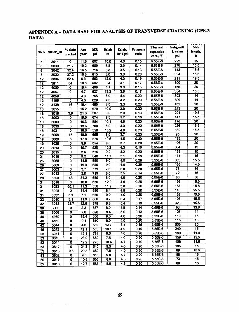
APPENDIX A - DATA BASE FOR ANALYSIS OF TRANSVERSE CRACKING (GP8-3DATA)

e;. slabs Age MR Dslab Eslab, Poisson's Thermal Subarade SlabState SHRP_ID expansion k-value length,cracked year psi in IOA6 psi ratio

cod., IF psi ft5 3011 0 11.6 607 10.0 4.0 0.15 5.55E-6 222 156 3030 21.7 19.2 609 8.5 3.9 0.14 5.55E-6 276 15.56 3042 12.4 16.5 714 8.8 3.5 0.13 5.55E-6 143 15.58 3032 37.2 16.3 615 8.0 3.8 0.20 5.55E-6 394 15.512 3804 62.4 6.3 553 12.0 4.0 0.19 5.55E-6 211 19.512 3811 64 18.6 502 9.4 3.1 0.17 5.55E-6 300 2012 4000 0 18.4 469 8.1 3.6 0.15 5.55E-6 158 2012 4057 0 4.7 537 13.3 3.8 0.17 5.55E-6 354 15.512 4059 0 4.0 765 6.0 4.4 0.20 5.55E-6 303 1412 4109 0 4.0 629 7.0 4.2 0.20 5.55E-6 300 1412 4138 16 18.4 480 8.0 3.3 0.20 5.55E-6 182 2013 3015 0 15.2 679 10.0 3.9 0.20 5.55E-6 243 2013 3018 3.9 21.3 507 9.9 2.0 0.13 5.55E-6 201 19.518 3002 0 19.5 674 9.5 5.7 0.18 5.55E-6 147 15.518 3003 0 16.3 584 10.1 4.8 0.20 5.55E-6 176 2018 3030 0 13.6 700 8.0 4.0 0.20 5.55E-6 226 15.518 3031 0 18.0 558 10.2 4.9 0.20 5.55E-6 139 15.519 3006 16 18.9 655 8.5 3.7 0.20 5.55E-6 95 2019 3009 8 17.8 576 10.6 4.5 0.20 5.55E-6 135 2019 3028 0 9.8 654 9.5 3.7 0.20 5.55E-6 106 2020 3013 0 10.7 520 10.2 4.3 0.16 5.55E-6 304 1520 3015 0 3.6 515 9.2 4.2 0.20 5.55E-6 129 1521 3016 0 9.2 640 11.7 5.1 0.18 5.55E-6 174 1526 3068 0 14.6 650 9.0 4.0 0.20 5.55E-6 300 15.526 3069 0 19.9 650 9.0 4.0 0.20 5.55E-6 165 14.527 3003 0 3.7 579 7.6 5.0 0.20 5.55E-6 78 1527 3013 0 3.0 719 8.0 5.5 0.14 5.55E-6 72 1529 5393 48 31.2 650 8.0 4.0 0.20 5.55E-6 88 3031 3018 0 10.0 650 12.0 4.0 0.20 5.55E-6 159 15.531 3023 65.1 11.3 556 11.9 3.8 0.16 5.55E-6 167 15.531 3028 0 14.4 550 8.4 4.9 0.20 5.55E-6 110 15.531 3033 3.1 7.1 650 9.0 4.0 0.20 5.55E-6 132 15.532 3010 3.1 11.9 606 9.7 3.4 0.17 5.55E-6 105 15.532 3013 21.7 12.9 579 8.3 5.4 0.19 5.55E-6 323 15.538 3005 0 8.3 587 8.0 4.8 0.14 5.55E-6 83 13.838 3006 0 7.8 620 8.4 5.0 0.13 5.55E-6 125 1440 4160 0 15.4 650 9.0 4.0 0.20 5.55E-6 110 1540 4162 0 9.4 650 9.0 4.0 0.20 5.55E-6 118 1542 3044 0 4.6 580 12.7 3.4 0.16 5.55E-6 505 2046 3012 3 12.1 555 10.1 4.9 0.19 5.55E-6 240 1553 3011 0 12.1 784 9.0 4.0 0.20 5.55E-6 180 11.453 3013 0 23.9 650 7.8 4.0 0.20 5.55E-6 159 15.553 3014 0 12.2 770 10.4 4.7 0.19 5.55E-6 108 11.553 3812 0 24.3 540 9.0 4.0 0.20 5.55E-6 195 1553 3813 9.3 29.3 650 7.8 4.0 0.20 5.55E-6 89 15.583 , 3802 0 9.8 618 9.8 4.7 0.20 5. 55E-6 88 1589 3015 0 10.8 655 8.0 4.0 0.20 5.55E-6 73 1689 3016 0 12.7 585 8.6 4.6 0.20 5.55E-6 89 16

Widened If widened TiedIf tied,

Base BaseDbaseState SHRP_ID lane? distance-to-edge shoulder? stabilized? bonded? Ebase, psi

(YorN) in (YorN)AGGIkI

(YorN) (U orB)in

5 3011 0 N 0 Y U 6.9 10000006 3030 0 y 0.1 Y U 4.3 10000006 3042 0 N 0 Y U 5.5 10000008 3032 0 Y 0.1 Y U 5.0 200000012 3804 0 N 0 Y U 7.6 200000012 3811 0 N 0 Y U 7.6 20000012 4000 0 N 0 y U 5.7 20000012 4057 0 N 0 N 7.0 2000012 4059 0 Y 0.1 N 9.8 20000012 4109 0 Y 0.1 N 9.8 20000012 4138 0 Y 0.1 Y U 5.9 20000013 3015 0 y 0.1 Y U 6.0 20000013 3018 0 Y 0.1 Y U 6.8 100000018 3002 0 N 0 N 7.0 3000018 3003 0 Y 0.1 Y U 6.5 10000018 3030 0 Y 0.1 Y U 5.4 45000018 3031 0 N 0 Y U 5.6 45000019 3006 0 N 0 Y U 5.0 100000019 3009 0 y 0.1 y U 5.7 20000019 3028 0 y 0.1 Y U 5.0 200000020 3013 0 y 0.1 Y U 5.0 100000020 3015 0 N 0 y U 5.2 45000021 3016 0 Y 0.1 N 7.0 3000026 3068 0 N 0 Y U 5.0 45000026 3069 0 y 0.1 Y U 5.0 20000027 3003 y 24 N 0 N 6.0 3000027 3013 Y 24 Y 0.1 N 6.0 3000029 5393 0 N 0 N 4.0 3000031 3018 0 y 0.1 Y U 6.0 20000031 3023 0 N 0 Y U 5.0 100000031 3028 0 y 0.1 y U 4.0 10000031 3033 0 Y 0.1 Y U 5.8 45000032 3010 0 y 0.1 Y U 6.6 100000032 3013 0 y 0.1 y U 4.7 100000038 3005 0 N 0 N 3.0 3000038 3006 0 Y 0.1 N 5.0 3000040 4160 0 N 0 Y U 4.0 040 4162 0 N 0 y U 4.0 45000042 3044 0 Y 0.1 N 9.0 3000046 3012 0 Y 0.1 N 5.0 3000053 3011 0 N 0 N 5.8 3000053 3013 0 Y 0.1 N 4.0 3000053 3014 0 N 0 N 6.0 3000053 3812 0 N 0 N 3.0 3000053 3813 0 N 0 N 3.4 3000083 3802 0 N 0 N 7.0 3000089 3015 0 N 0 N 10.0 3000089 3016 0 N 0 N 10.0 30000