Embed Size (px)
Citation preview

Efficient and Accurate Power Delivery and Inductance Analysis
Charlie Chung-Ping ChenUniversity of Wisconsin
http://vlsi.ece.wisc.edu

Outline• Motivation• Inductance Analysis• Efficient Power Delivery Simulation
Techniques– INDUCTWISE– HIPRIME– TLMADI
• Experimental Results• Conclusion

Motivation: Trend of VLSI Technology
� Increasing power dissipation� Decreasing supply voltage
Power Supply Voltage Roadmap
0.8
0.9
1
1.1
1.2
1.3
1.4
1.5
1.6
1.7
1.8
1999 2000 2001 2002 2003 2004 2005
Volt
Vdd maxVdd min
* Data from International Technology Roadmap for Semiconductors (ITRS)
Power Dissipation Roadmap
90
100
110
120
130
140
150
160
170
1999 2000 2001 2002 2003 2004 2005
Wat
t
Power max

Motivation: Why Power Grids Analysis?
roughly proportional to L(I x f) = L (P x f / Vdd )� I : consuming current� f : clock frequency� P : power dissipation� Vdd : supply voltage
• Power delivery quality becomes a critical issue
� Other noises such as resonance and electromigration also affect power grid reliability
� Power fluctuation sources increase significantly� IR-drop: ∆V = I x R = (P /Vdd ) x R� L di/dt: ∆V = L di/dt

Motivation: Power Grids Analysis Challenges
• More than 40-million transistors on a chip• Sparse direct method takes super linear time
to solve a matrix.– Introduce a large amount of fill-ins– Slow and huge memory requirement – SPICE takes 6 hours to finish DC analysis for
an 80,000-node circuit– How about more than millions?

Power Grid Modeling
Vcc
On-Chip resistance and inductance
Gates Gate Capacitance & DECAPS
Power Supply
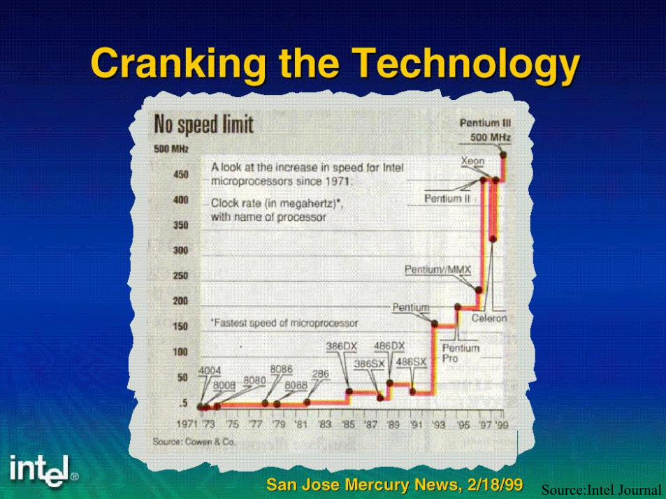
Source:Intel Journal

Inductance Effects Emerging
f
Ljω
Cjω/1
R
• Skin Effect
• Proximity Effect
• Loop Inductance Variation
• Return Paths
Impedencef
R
L
Impedence

Skin Effects• Skin Depth
µσπδ
f1=
e/1
I
CuAl
um
f

Inductive vs. Capacitive Coupling Noises
sV V V V GVVGWith inductance Without inductance
1000um M7
40fF gCap

Where are the return paths?
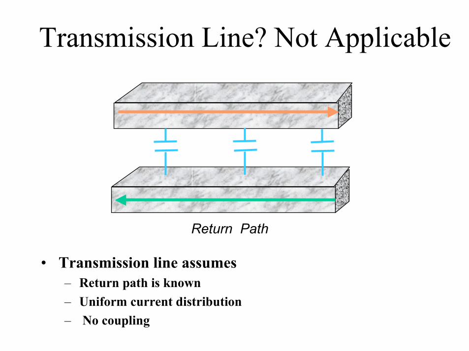
Transmission Line? Not Applicable
• Transmission line assumes– Return path is known – Uniform current distribution– No coupling
Return Path

Power Delivery
iI
kj
NodeVoltage
BranchCurrent 1iV
Width
iLLength
Pad
iwPad
GroundNetwork
ExternalCurrent
2iV

Inductance Modeling and Simulation Issues
• Loop inductance is hard to find due to complicated return paths issues– Partial Element Equivalent Circuits (Ruehli 1972)– FastHenry: Use RL to find the effective loop inductance in
frequency domain (J. White, et al , MIT)
• Too many small coupling terms– Every non-orthogonal conductor have mutual inductance
terms– Kill the performance of sparse matrix based solver– Randomly throw out smaller terms will causes non-passive
circuit

PEEC (Partial Equivalent Element Circuit)
d w
tl
• Only geometry dependent, PEEC generate SPICE-compatible partial inductance (instead of loop inductance) and capacitance
• Valid through a wide range of frequency. [Ruehli 72]

Our Contribution
• Develop an accurate, efficient, and guarantee stability inductance extraction and sparsification tool for both on-chip and packaging application
• Develop an efficient time-domain PEEC solver tune for inductance simulation

Long Range Inductance Effects
• LMatrix (far/near=16%) (Unit:pH/10um)– M7: 5.90675 3.7651 2.66996 2.07728 1.69795 1.43288
1.23712 1.08682 0.967989 – M5: 2.21793 2.12341 1.91089 1.67618 1.46486 1.2872
1.14074 1.02009 0.920046
M7
M5

1
0.56
(um)0.39
0
50
100
150
2
3
4
5
�������������� ������ ������
��� ������������������������� �������
�������������������

L-1 and K-Method (A. Devagon I.B.M and W. Dai)
• LMatrix (far/near=16%) (Unit:0.1 pH/um)– M7: 5.90675 3.7651 2.66996 2.07728 1.69795 1.43288
1.23712 1.08682 0.967989 – M5: 2.21793 2.12341 1.91089 1.67618 1.46486 1.2872
1.14074 1.02009 0.920046• L-1Matrix (far/near=0.8%) (Diagonal Dominate) (Can delete smaller terms and passive)
– M7: 0.299863 -0.161026 -0.00559067 -0.00646425 -0.00335869 -0.00230476-0.00176532 -0.00146807 -0.00263693
– M5: -0.0345231 -0.0119699 -0.0049231 -0.00208736 -0.00122399 -0.000925889-0.000820881 -0.000814121 -0.00173737
M7
M5

(a) (b) (c)
!"��#� �$��%&�����������'���������
K-Method INDUCTWISE Halo Method(K. Sherperd)

1
0.56
(um)0.39
0
50
100
150
2
3
4
5
Non-Diagonal Dominate Concern for K-method
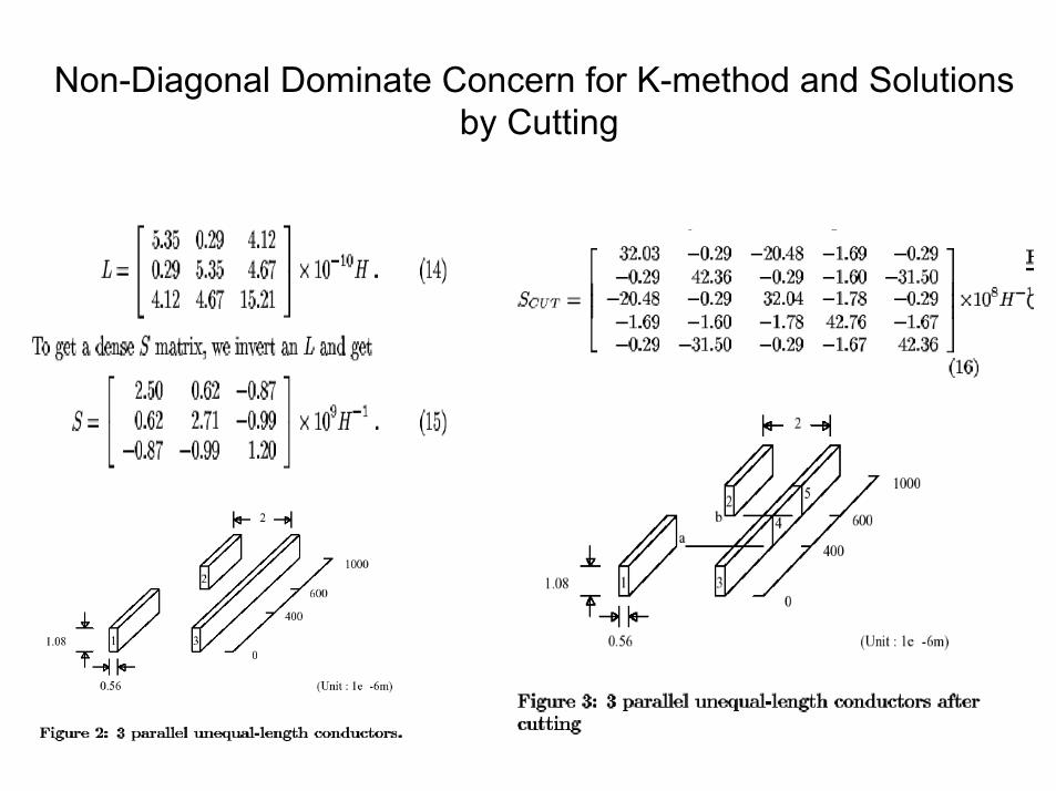
Non-Diagonal Dominate Concern for K-method and Solutions by Cutting

0 0
0
LAl−
TA l
Modified Nodal Analysis Example
Iin
C1
C2
R1
R2L1
1 2
[ ]1L=L
=
2
1
C00C
C
=
2
1
R100R1
G
[ ]ini I=I
−=
1011
A g
−=
1011
Ac
[ ]01=A l
[ ]01=A iMNA Equation:AA gg GT AA gg CT
[ ]in
L
2
1
1
211
11
L
2
1
211
11
I001
IVV
L000CCC-0C-C
IVV
001-0R1R1R1-1R1-R1
−=
++
+
• Ai−
0

Modified Nodal Analysis (MNA)
• Good for general circuits (RLC and current sources here)
• Extra current variables ( Il ) required• Non-positive definite
IA
IVAA
IV
AAAA
i
Ti
l
ncc
l
n
l
lgg
LCG
−=
+
−
•
000
0
TTT

Solve RLC circuit by NA
• Modified Nodal Analysis (MNA)
– Indefinite ⇒cannot use CG• Rewrite in Nodal Analysis (NA) format
– Use Trapezoidal approximation– Substitute (2) into (1) and eliminate Il– Obtain Avn=b, where A is s.p.d.
( )( )21
000
0
TTT
IA
IVAA
IV
AAAA
i
Ti
l
ncc
l
n
l
lgg
LCG
−=
+
−
•
)( 1 VAI nll L−•
=

Nodal Analysis (NA)
• MNA can reduced to NA format by� Trapezoidal approximation � Inverse L and eliminate Il� Obtain Avn=b, where A is s.p.d.
• Good for circuit with RLC and current sources and compatible with the K-method
• No extra current variables needed• Symmetric positive definite and diagonally
dominant ⇒ Use PCG iterative method and incomplete Cholesky decomposition
2)(')(')()( txttx
ttxttx +∆+=
∆−∆+

Iterative Methods
• Classifications– Stationary methods: Jacobi, gauss-Seidel, SOR, SSOR
(relatively slow)– Nonstationary methods: CG, MINRES, GMRES, CGNE
• GMRES – Has to store previous search directions to obtain next orthogonal
direction. Memory required– Useful for non-symmetric matrices
• Conjugate gradient (CG)– Guarantee n-iteration convergence– Symmetric positive definite required– Unlike GMRES, no need to store previous directions.

Conjugate Gradient• Solution for ⇔
Minimize
• Minimal happens when the gradient of the quadratic form is equal to zero
• Algorithm:– Start at an initial guess– Find the search direction– Find the minimum gradient point
along this direction– Find the next direction and
continue the process
xb-Ax x TT
21(x) =f
bAx =

Conjugate Gradient• Any two search directions are A-orthogonal <xi,
Axj>=0 for i≠j• No direction is repeated ⇒ convergence in n
iterations guarantee, where A is an nxn matrix
• Convergence of CG:
– Where κ=|λmax|/|λmin| is the condition number– x* is the exact solution, and xm is the solution in the
mth iteration– The closer κ →1, the less iterations need to converge
A0*
m
Am* ||xx||
1κ1κ||xx|| −
+−≤−

Preconditioning Technique
• Reduce the condition number κ to make it converge faster
• Instead of solve Ax=b, solving M-1Ax=M-1b• Try to make M ≅ A. M-1 A ≅ I, then the condition
number of the new system is closer to 1 than the original system.
• Use incomplete LU decomposition instead of inversing M

0 5 10 15 20
0
5
10
15
20
nz = 580 5 10 15 20
0
5
10
15
20
nz = 580 5 10 15 20
0
5
10
15
20
nz = 95
Preconditioners (Continued)• Incomplete LU decomposition:
Find A = LU + E
• ILU(1) – First level fill-in factorization: decomposed based on the
topology of (L0U0)
L0U0 L1 U1

�������������� ������� ����

Inductance SparsficationPerformance
# of Exact Solution Reluctance MethodCond. Density Ext. Time(s) Simu. Time(s) Ext. Time(s) Simu. Time(s)
154 11.40% 2.23 10.33 0.77(2.9x) 7.20(1.4x)538 3.40% 26.32 119.65 2.76(9.5x) 27.38(4.4x)989 1.80% 89.81 623.37 5.18(17.3x) 54.20(11.5x)
1367 1.10% 250.75 3565.71 9.17(27.3x) 95.79(37.2x)

Near End versus Far End Noise ErrorCompare to Shell Preconditioning

Near End versus Far End Noise ErrorCompare to Shell Preconditioning

Conclusion
• Develop an accurate, efficient, and guarantee stability inductance extraction and sparsfication tool for both on-chip and packaging application
• Develop an efficient time-domain PEEC solver tune for inductance simulation
• The total speed up over exact SPICE3 simulation is around 100-400X

Thank you

Accuracy for Aggressor
0.90.95
11.05
1.11.15
1.21.25
1.31.35
1.4
0 5 10 15 20
Exact Solution
k=1, x=1.0k=1, x=0.5
k=1, x=0.5Step Responsefor Aggressor
• Small window is good enough for the aggressor.
• Larger extended search factor helps the accuracy on aggressor.

Speed up of our Method

Accuracy for Victim
• Larger window is necessary.
• Extended search factor is not critical for the accuracy of victims.
-0.06
-0.04
-0.02
0
0.02
0.04
0.06
0.08
0.1
0 5 10 15 20
Exact Solutionk=3, x=0.5
k=2, x=0.5k=1, x=0.5
k=3, x=0.5Step Response
for Victim

Enhanced K Method by Group Calculation

Multiple Aggressors : Even mode vs. Odd mode (cont’d)
• 3 parallel conductors (1000um)
• Act1 : Single aggressor
• Act2_even : 2 aggressors are activated in even mode
• Act2_odd : 2 aggressors are activated in odd mode
• While the coupling noise is decreased in odd mode, it is increased in even mode
* The time axis in this graph is not perfectly aligned for each case
Multiple Aggressors : Even mode vs. Odd mode
-4.00E-01
-2.00E-01
0.00E+00
2.00E-01
4.00E-01
1.40E-09 1.50E-09 1.60E-09 1.70E-09 1.80E-09 1.90E-09 2.00E-09 2.10E-09 2.20E-09 2.30E-09 2.40E-09
Time (sec)
Vol
tage
(V)
Act1
Act2_even
Act2_odd
15.80.026Act2(odd)
198.40.326Act2(even)
Reference0.164Act1
Normalized(%)
Voltage(V)
Mode

Literature Overview• Hierarchical analysis of power distribution network (Sachin-DAC2000)
– Decoupled linear and nonlinear simulation (only for RC circuit)– Divide and Conquer simulation for large scale simulation– Sparsfication to reduce memory usage
• Efficient large-scale RLC power grid analysis based on preconditioinedKrylov-subspace iterative methods (Chen-DAC2001)
– Incomplete cholesky decomposition and iterative method to reduce fillins and number of iterations -> over 100X speed up
• Multigrid-like technique for power grid analysis (Sani R. Nassif- ICCAD2001)– Reduce the grids to a coarser structure, and the solution is mapped back to the
original grid

Partial Self and Mutual Inductance Extraction (Grover)
++−
++
−+
+
ls
ls
sl
slmlpHM
ktw
lmlpHL
Grover
mutual
self
2
2
2
2
11ln)(2.0~)(
5.02ln)(2.0~)(
:
µ
µ
l
l
w
st
minallltwswhensllpHM
twllpHL l
smutualself
µ ,),( ,
,12ln2.0~)( ,5.02ln2.0~)(
<<+
+−
+
+

Partial Inductance Extractionfor Skewed Parallel-Case 1
ofindepent is ,0 0 ))()((5.0~)( ,0
))(((5.0~)( , 0 ))()((5.0~)( , 0
sMdorswhenMMMMpHMdm
MMMpHMdMMMMpHMd
ij
dmdlddmlij
mlmlij
dmdlddmlij
>=
+−+<<−
+−=
+−+>
++−++
+
++++
l
m
ds

Partial Inductance Extractionfor Skewed Parallel-Case 2
))((5.0~)( ,0))()((5.0~)( ,0
mlmlij
edemdmij
MMMpHMdeMMMMpHMde
−
++
−+=
+−+<>
l
mds
e

Loop Inductance definition
LP1,1S1 S2
∑∑= =
=3
1
3
1,1
i jjis ML
LP2,2
LP3,3 LP4,4
LP5,5
LP6,6
∑∑= =
=6
4
6
4,2
i jjis ML
∑∑= =
=3
1
6
4,2,1
i jjiss MM