Embed Size (px)
Citation preview
Stochastic Systems
arXiv: arXiv:0000.0000
CHATTERING AND CONGESTION COLLAPSE IN AN OVERLOADSWITCHING CONTROL
BY OHAD PERRY∗ AND WARD WHITT†
Northwestern University∗ and Columbia University†
Routing mechanisms for stochastic networks are often designed to pro-duce state space collapse (SSC) in a heavy-traffic limit, i.e., to confine thelimiting process to a lower-dimensional subset of its full state space. In a fluidlimit, a control producing asymptotic SSC corresponds to an ideal slidingmode control that forces the fluid trajectories to a lower-dimensional slidingmanifold. Within deterministic dynamical systems theory, it is well knownthat sliding-mode controls can cause the system to chatter back and forthalong the sliding manifold due to delays in activation of the control. For theprelimit stochastic system, chattering implies fluid-scaled fluctuations thatare larger than typical stochastic fluctuations.
In this paper we show that chattering can occur in the fluid limit of a con-trolled stochastic network when inappropriate control parameters are used.The model has two large service pools operating under the fixed-queue-ratiowith activation and release thresholds (FQR-ART) overload control whichwe proposed in a recent paper. The FQR-ART control is designed to produceasymptotic SSC by automatically activating sharing (sending some customersfrom one class to the other service pool) once an overload occurs. We havepreviously shown that this control is effective and robust, even if the servicerates are less for the other shared customers, when the control parameters arechosen properly. We now show that, if the control parameters are not cho-sen properly, then delays in activating and releasing the control can causechattering with large oscillations in the fluid limit. In turn, these fluid-scaledfluctuations lead to severe congestion, even when the arrival rates are smallerthan the potential total service rate in the system, a phenomenon referred to ascongestion collapse. We show that the fluid limit can be a bi-stable switchingsystem possessing a unique nontrivial periodic equilibrium, in addition to aunique stationary point.
1. Introduction. In this paper we study the fluid limit of a stochastic sys-tem comprised of two service pools, each having its own arrival process and ownqueue. The system is operating under the fixed-queue-ratio with activation and re-lease thresholds (FQR-ART) overload control (specified in §2.1 below), which wasdeveloped in [28, 32]. The control is designed to automatically switch on sharing(serving some customers from the other pool) when an unexpected overload oc-curs, and switch off sharing when the overload incident is over, based only on the
MSC 2010 subject classifications: Primary 60K25, 34C25, 34C55; secondary 60F17, 37G15Keywords and phrases: stochastic networks, fluid models, overload control, congestion collapse,
switching dynamical systems, bi-stability, periodicity
1
2 PERRY AND WHITT
observed queue lengths. While the control is switched on, it aims to hold the twoqueues nearly fixed at some pre-specified ratio. From a many-server asymptoticperspective, the fixed-queue-ratio goal is to produce state space collapse (SSC).
It is significant that when the control parameters are chosen appropriately, thecontrol is both effective and robust. In particular, it is successful in automaticallyswitching on and off as needed, and in producing the desired SSC (again, auto-matically), even under unrealistically-extreme conditions; see [31] for key theory,involving an averaging principle, and §4.3 in [33] for important examples.
Nevertheless, in some extreme cases a performance degradation was demon-strated via simulation in [32]. More specifically, with highly inefficient sharing(the service rate is much less for the other customers), if the control parametersare badly-chosen, a system that is recovering from an overload incident, and is nolonger overloaded, may get stuck in an oscillatory behavior that is due to unin-tended on-and-off switchings of the control. We now provide mathematical analy-sis that establishes key properties of this oscillatory behavior and provides a way toapproximately quantify it. In [32] we developed a fluid approximation that can beused, in addition to simulation, to ensure that the bad behavior does not occur. Nev-ertheless, it is important to carefully study the limitations of controls. The insightsgained should be useful for studying other overload controls.
A Switching Control. Most of the literature on control of queueing networksdeals with ongoing operations, in which the control is operating continuously. Typ-ically, it is also assumed that the arrival rates and total service capacity are known.However, here we are considering the control in [32] which automatically switcheson and off, as was briefly described above. The fluid analysis we perform thus fallswithin the settings of (deterministic) switching dynamical systems [23].
A simple example of a switching system is the description of heated space. Ifthe target temperature is set to be T ◦F , then a thermostat should turn the heating onwhenever the temperature drops below level T , and off when it reaches the targetagain. The ideal dynamic system’s description then has two phases: The reaching(transient) phase, which describes the system until the temperature reaches levelT , and the “sliding” phase, in which the temperature remains fixed (“slides”) atT . Since heat is lost continuously, a true sliding phase requires that the thermostatswitch the heating on and off infinitely-many times during any time interval. Inreality, a hysteresis control is employed, namely, the thermostat turns the heat onwhen the temperature reaches some level T` < T , and off when the temperaturehits some level Th > T . Hence, a more realistic description of the correspondingdynamical system has the temperature chatter about level T , with this chatteringbeing faster and smaller the more accurate the thermostat is. If the chattering is suf-ficiently small and fast, then the hysteresis dynamics approximate the ideal slidingphase quite well.
CHATTERING IN OVERLOAD CONTROL 3
The queueing system we consider here has important similarities with the heat-ing system describe above in that it is designed to “slide” on some region of itsstate space. More importantly, as we explain below, many other control mecha-nisms for queueing systems are designed for this purpose. The difference betweenthe “ideal” sliding and the dynamics that are experienced in practice must be takeninto account so as to avoid the harmful phenomena described here.
State Space Collapse, Sliding Motion and Chattering. Asymptotic SSC inheavy-traffic limits is often a key step in developing effective (e.g., asymptoticallyoptimal) controls for multidimensional stochastic networks; e.g., [4, 14, 15, 31,34, 41, 43, 49]. (Related ideas date back to [46], but the systems there are un-controlled.) As the term suggests, SSC means that the limit process is of a lowerdimension than the prelimit process. More precisely, if SSC holds, then the limitprocess “collapses” (i.e., is confined) to a lower dimensional subset of its full statespace. It is significant that SSC is often not only a mathematical tool that is em-ployed to simplify asymptotic analysis, but rather, as in [31], SSC may be a goalof the control. We elaborate on the relation of SSC to optimal control in §9 below.See also page 136 in [1].
In the context of a functional weak law of large numbers (FWLLN) or fluid limit,asymptotic SSC corresponds to the limiting deterministic fluid process exhibitinga sliding motion, i.e., all the fluid trajectories “slide” on a lower-dimensional sub-space, called a sliding manifold; see, e.g., §14.1 in [21] and §1.2.3 in [23]. In suchcases, the fluid limit often has discontinuous dynamics in its full state space; i.e.,it is governed by an ordinary differential equation (ODE) with a discontinuousright-hand side. The discontinuous dynamics is often avoided by assuming that theinitial condition is asymptotically on the sliding manifold and restricting attentionto the behavior of the limit on that region of the state space. However, if the initialcondition of the fluid limit is not on the sliding manifold, the fluid trajectory mustfirst go through a transient period before reaching the manifold; see Theorem 3 in[4] and the explanation preceding it. (We remark that sliding manifolds should notbe confused with the invariant manifolds in [4], which are defined to be the fixedpoints of the fluid limit. In particular, on the invariant manifold, the fluid trajec-tories are constant functions, whereas on a sliding manifold, the fluid limits mayexhibit a transitory behavior.)
An effective SSC control must therefore (i) pull the system to the sliding man-ifold without undue delay and (ii) ensure that the system remains on the slidingmanifold thereafter. For queueing networks, this may require specifying differentrouting rules for different regions of the state space - on and off the sliding man-ifold. For example, suppose that the state space S can be partitioned into threedisjoint subsetsM,M+ andM−, whereM is a sliding manifold, whileM+ andM− are “above” and “below”M. A sliding-mode control will direct trajectories
4 PERRY AND WHITT
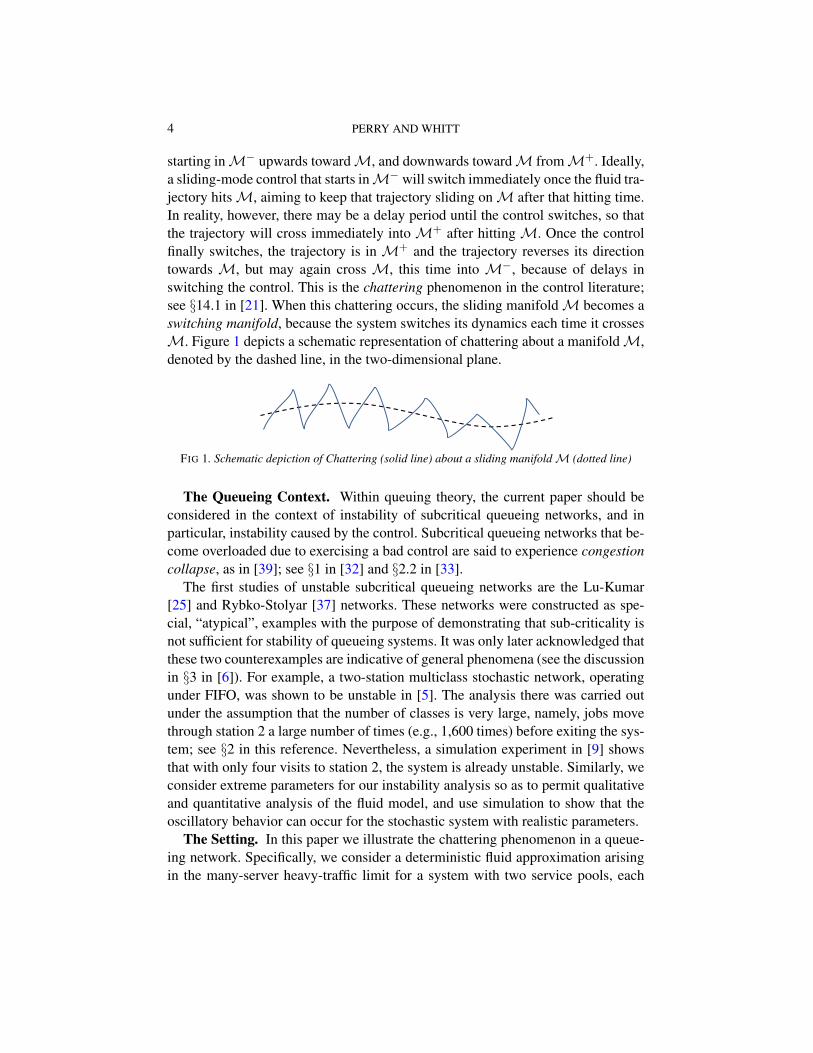
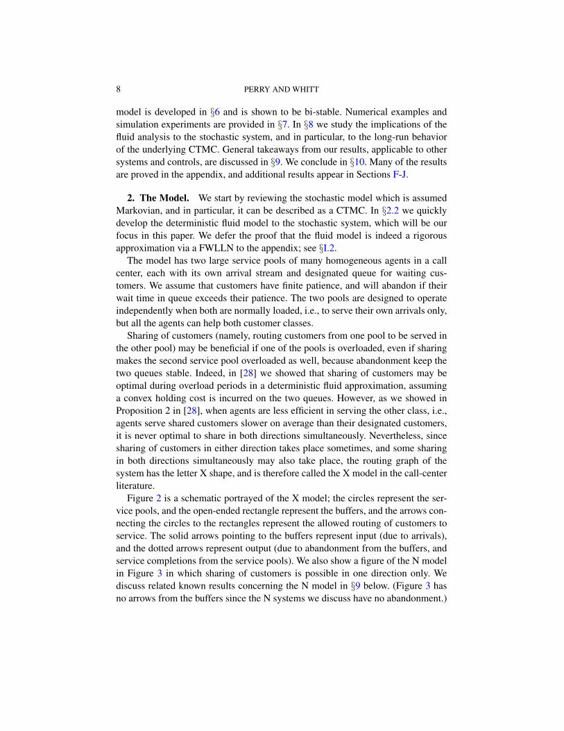
starting inM− upwards towardM, and downwards towardM fromM+. Ideally,a sliding-mode control that starts inM− will switch immediately once the fluid tra-jectory hitsM, aiming to keep that trajectory sliding onM after that hitting time.In reality, however, there may be a delay period until the control switches, so thatthe trajectory will cross immediately intoM+ after hittingM. Once the controlfinally switches, the trajectory is in M+ and the trajectory reverses its directiontowards M, but may again cross M, this time into M−, because of delays inswitching the control. This is the chattering phenomenon in the control literature;see §14.1 in [21]. When this chattering occurs, the sliding manifoldM becomes aswitching manifold, because the system switches its dynamics each time it crossesM. Figure 1 depicts a schematic representation of chattering about a manifoldM,denoted by the dashed line, in the two-dimensional plane.
FIG 1. Schematic depiction of Chattering (solid line) about a sliding manifoldM (dotted line)
The Queueing Context. Within queuing theory, the current paper should beconsidered in the context of instability of subcritical queueing networks, and inparticular, instability caused by the control. Subcritical queueing networks that be-come overloaded due to exercising a bad control are said to experience congestioncollapse, as in [39]; see §1 in [32] and §2.2 in [33].
The first studies of unstable subcritical queueing networks are the Lu-Kumar[25] and Rybko-Stolyar [37] networks. These networks were constructed as spe-cial, “atypical”, examples with the purpose of demonstrating that sub-criticality isnot sufficient for stability of queueing systems. It was only later acknowledged thatthese two counterexamples are indicative of general phenomena (see the discussionin §3 in [6]). For example, a two-station multiclass stochastic network, operatingunder FIFO, was shown to be unstable in [5]. The analysis there was carried outunder the assumption that the number of classes is very large, namely, jobs movethrough station 2 a large number of times (e.g., 1,600 times) before exiting the sys-tem; see §2 in this reference. Nevertheless, a simulation experiment in [9] showsthat with only four visits to station 2, the system is already unstable. Similarly, weconsider extreme parameters for our instability analysis so as to permit qualitativeand quantitative analysis of the fluid model, and use simulation to show that theoscillatory behavior can occur for the stochastic system with realistic parameters.
The Setting. In this paper we illustrate the chattering phenomenon in a queue-ing network. Specifically, we consider a deterministic fluid approximation arisingin the many-server heavy-traffic limit for a system with two service pools, each
CHATTERING IN OVERLOAD CONTROL 5
having its own arrival process and designated queue, that is operating under theFQR-ART overload control which we suggested in [32]. Normally, the two poolsprocess work from their designated queues only. However, when an overload oc-curs due to an unexpected shift in the arrival rates, the control automatically iden-tifies which queue should receive help and sharing begins, so that jobs from theoverloaded queue are routed to both service pools, according to a routing rule thatwill be specified below.
The overload control was created for two call centers that normally operate sepa-rately, but might benefit by assisting each other to respond to unexpected overloadsby temporarily serving some of the other customers. Given this call center motiva-tion, we refer to pools of agents and the customers served in the other (not desig-nated) pool as shared customers. When sharing is activated, the goal is to maintainthe two queues nearly fixed at a pre-specified ratio during overload periods that isoptimal with an appropriate cost formulation; see [28].
We showed that sharing can be effective even if sharing is inefficient, i.e., theshared customers are served at a slower rate. Since there is the possibility of per-formance degradation if there is too much sharing, it is necessary to choose thecontrol parameters appropriately. The root cause of the chattering discussed here isindeed the combination of excessive inefficient sharing and poorly chosen controlparameters. To avoid excessive simultaneous sharing of customers in both direc-tions (“two-way sharing,”see §4.1 in [28]), sharing with pool 1 helping queue 2is activated only if the number of shared customers in pool 2 is below a certain(small) threshold, and similarly in the other direction. This latter restriction cancause delays in activating sharing when the direction of overload switches. Onceactivated, the control aims to produce asymptotic SSC by confining the queues toa certain region of the state space in the fluid limit [31]. In the fluid limit, this SSCtranslates to sliding motion on one of two sliding manifolds, each associated withone direction of sharing. We elaborate in §2 below.
When sharing is inefficient and the control parameters are not chosen appro-priately, delays in activating the control can cause so much chattering that thefluid trajectory hits both sliding manifolds, without remaining in either, leadingto complex chattering behavior. Here the chattering manifests itself in periodic os-cillations, which lead to inefficient utilization of the service capacity. In turn, theinefficient utilization of agents creates severe overloads, even though the arrivalrates we consider are smaller than the potential service capacity.
Chattering in sliding-mode controls is a well-known phenomenon in determin-istic control theory. Indeed, chattering is considered to be the natural “state ofaffairs”, whereas perfect sliding motion is considered ideal and unrealistic; e.g.,§14.1 in [21]. Accordingly, even though we focus on a single system that operatesunder a specific control, our results have broader relevance. In particular, similar
6 PERRY AND WHITT
phenomena should be expected to occur with other SSC-inducing controls whenthere are deviations from ideal modeling assumptions, such as stationarity, or “con-venient” initial conditions and control settings.
Switching Dynamical Systems. The chattering found in the fluid model im-plies that the ODE governing the evolution of the fluid trajectories switches when-ever the control is activated or released. Therefore, the appropriate fluid modelx := {x(t) : t ≥ 0} for the stochastic system is a switching dynamical systemx = fσ(x)(x), where σ(x) achieves a finite set of values, fi is a continuous func-tion for each value i of σ, but the function fσ is discontinuous [23]. As the notationsuggests, the switching epochs are state dependent (depending only on the value ofthe solution x), so that the ODE is autonomous (time-homogeneous).
The framework of switching systems in general, and of systems with slidingmotion in particular, is outside the classical ODE and dynamical-systems theory,because the right-hand side function fσ is not continuous, and so it is not locallyLipshcitz. Hence, the conditions of the Picard-Lindelof theorem, ensuring the ex-istence of a unique solution to the ODE, are not satisfied. In general, the existenceof a unique solution to a switching system with no sliding motion can only hold inthe Caratheodory sense, namely, such a solution is an absolutely-continuous func-tion that satisfies the ODE almost everywhere; see [23]. A solution with a slidingmotion is generally considered to hold in the Filippov sense [12], In [30, 31] wehave proved that a unique solution exists for the fluid limit of our system duringsliding motion via a stochastic averaging principle (i.e., the control achieves thedesired asymptotic SSC).
Analytical Contribution. In addition to exposing the chattering behavior dis-cussed above, our current work has important analytical contributions. We empha-size at the outset that the derivation of the fluid model, which will also be shownto be the FWLLN in §I.2, and its quantitative analysis is relatively standard. Thestronger analytical contributions lie in the nontrivial qualitative analysis of the fluidmodel. Specifically, we provide sufficient conditions for chattering to lead to end-less oscillations, and prove the existence of a periodic equilibrium. Furthermore,we provide a simple algorithm to efficiently analyze the system for any given initialcondition.
It is known that even seemingly simple switching systems can experience chaotic-like behavior, e.g., have infinitely-many periodic equilibria that are dense in thestate space, and exhibit high sensitivity to perturbations of the initial condition(popularly known as “the butterfly effect”); see, e.g., [8, 11]. Such systems areclearly unamenable to long-run analysis. Even fluid models of uncontrolled sys-tems can have uncountably-many periodic equilibria [24]. However, numerical ex-periments suggest that our system has at most one periodic equilibrium, and that itis bi-stable, i.e., any fluid trajectory can have long-run behavior of only two kinds:
CHATTERING IN OVERLOAD CONTROL 7
either it converges to the periodic equilibrium, or else it converges to the uniquestationary point (which is therefore asymptotically stable).
To conduct a more complete study of the (bi)stability properties of the fluidmodel, we create an approximation to the fluid system. (Note that “stability” heredoes not refer to the prelimit queueing system which is always stable due to as-sumed abandonment.) For that approximating dynamical system we show that alloscillating solutions must converge to the unique periodic equilibrium (of the ap-proximating system), while all other solutions converge to the unique stationarypoint, which is the same as that of the fluid limit. In particular, the approximatingsystem is bistable.We conjecture that the same is true for the fluid limit (Conjecture5.1 below), and support this conjecture by numerical experiments in §7.
To summarize, we develop and analyze two layers of approximations, one beingthe fluid limit, which approximates the stochastic system, and the other being anapproximating dynamical system which serves as a simplified approximation to thefluid limit, whose qualitative behavior is easier to characterize.
Implications of the Fluid Analysis to the Stochastic System. A straightfor-ward implication of our result that the fluid limit may oscillate indefinitely is thatthe prelimit stochastic systems can experience congestion collapse. Moreover, thefluid limit may oscillate, even though the stochastic system in the pre-limit is anergodic continuous-time Markov chain (CTMC) and is therefore necessarily ape-riodic with a unique equilibrium (stationary) distribution. Since the CTMC con-verges to its unique stationary distribution also for initial conditions that are asso-ciated with oscillatory fluid limits, one concludes that the convergence rate of theCTMC to stationarity must be prohibitively slow. We elaborate in §8.
Our fluid analysis also has indirect implications to the stochastic system. Specifi-cally, stochastic noise, which is not captured by the fluid approximation, may even-tually push the system into the oscillatory behavior, even if the system is unambigu-ously initialized in the attraction region of the stationary point. This suggests thatstochastic fluctuations can lead to fluid-scaled fluctuations. In addition, oscillationscan occur in the stochastic system even if its fluid limit does not possess a periodicequilibrium, and never oscillates. Therefore, studying the relatively simple fluidmodel is important for gaining insight into the dynamics of the stochastic system.See the examples in §7.3 below.
Organization. The rest of the paper is organized as follows. We describe thestochastic model and the control in §2. In §2.2 we explain how to construct a di-rect fluid model to approximate the system’s dynamics. The switching fluid modelis derived in §3. Qualitative analysis, including relevant equilibrium and stabilitynotions for dynamical systems, are rigorously defined and analyzed in §4. In §5 weshow that the fluid model can oscillate indefinitely and when it does we show thereexists a periodic equilibrium. The approximating dynamical system to the fluid
8 PERRY AND WHITT
model is developed in §6 and is shown to be bi-stable. Numerical examples andsimulation experiments are provided in §7. In §8 we study the implications of thefluid analysis to the stochastic system, and in particular, to the long-run behaviorof the underlying CTMC. General takeaways from our results, applicable to othersystems and controls, are discussed in §9. We conclude in §10. Many of the resultsare proved in the appendix, and additional results appear in Sections F-J.
2. The Model. We start by reviewing the stochastic model which is assumedMarkovian, and in particular, it can be described as a CTMC. In §2.2 we quicklydevelop the deterministic fluid model to the stochastic system, which will be ourfocus in this paper. We defer the proof that the fluid model is indeed a rigorousapproximation via a FWLLN to the appendix; see §I.2.
The model has two large service pools of many homogeneous agents in a callcenter, each with its own arrival stream and designated queue for waiting cus-tomers. We assume that customers have finite patience, and will abandon if theirwait time in queue exceeds their patience. The two pools are designed to operateindependently when both are normally loaded, i.e., to serve their own arrivals only,but all the agents can help both customer classes.
Sharing of customers (namely, routing customers from one pool to be served inthe other pool) may be beneficial if one of the pools is overloaded, even if sharingmakes the second service pool overloaded as well, because abandonment keep thetwo queues stable. Indeed, in [28] we showed that sharing of customers may beoptimal during overload periods in a deterministic fluid approximation, assuminga convex holding cost is incurred on the two queues. However, as we showed inProposition 2 in [28], when agents are less efficient in serving the other class, i.e.,agents serve shared customers slower on average than their designated customers,it is never optimal to share in both directions simultaneously. Nevertheless, sincesharing of customers in either direction takes place sometimes, and some sharingin both directions simultaneously may also take place, the routing graph of thesystem has the letter X shape, and is therefore called the X model in the call-centerliterature.
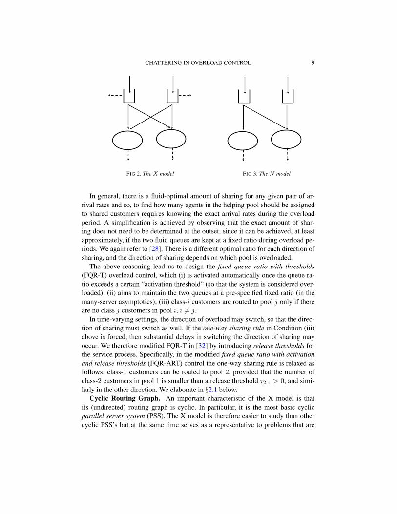
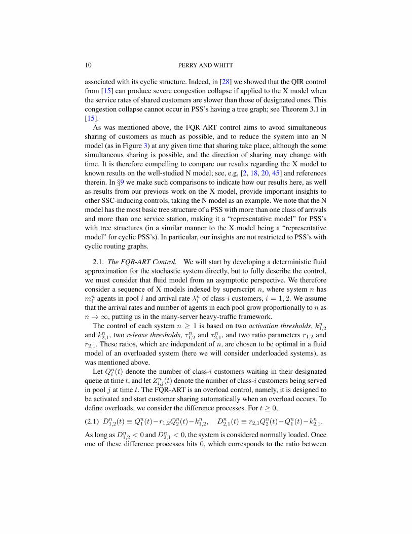
Figure 2 is a schematic portrayed of the X model; the circles represent the ser-vice pools, and the open-ended rectangle represent the buffers, and the arrows con-necting the circles to the rectangles represent the allowed routing of customers toservice. The solid arrows pointing to the buffers represent input (due to arrivals),and the dotted arrows represent output (due to abandonment from the buffers, andservice completions from the service pools). We also show a figure of the N modelin Figure 3 in which sharing of customers is possible in one direction only. Wediscuss related known results concerning the N model in §9 below. (Figure 3 hasno arrows from the buffers since the N systems we discuss have no abandonment.)
CHATTERING IN OVERLOAD CONTROL 9
FIG 2. The X model
FIG 3. The N model
In general, there is a fluid-optimal amount of sharing for any given pair of ar-rival rates and so, to find how many agents in the helping pool should be assignedto shared customers requires knowing the exact arrival rates during the overloadperiod. A simplification is achieved by observing that the exact amount of shar-ing does not need to be determined at the outset, since it can be achieved, at leastapproximately, if the two fluid queues are kept at a fixed ratio during overload pe-riods. We again refer to [28]. There is a different optimal ratio for each direction ofsharing, and the direction of sharing depends on which pool is overloaded.
The above reasoning lead us to design the fixed queue ratio with thresholds(FQR-T) overload control, which (i) is activated automatically once the queue ra-tio exceeds a certain “activation threshold” (so that the system is considered over-loaded); (ii) aims to maintain the two queues at a pre-specified fixed ratio (in themany-server asymptotics); (iii) class-i customers are routed to pool j only if thereare no class j customers in pool i, i 6= j.
In time-varying settings, the direction of overload may switch, so that the direc-tion of sharing must switch as well. If the one-way sharing rule in Condition (iii)above is forced, then substantial delays in switching the direction of sharing mayoccur. We therefore modified FQR-T in [32] by introducing release thresholds forthe service process. Specifically, in the modified fixed queue ratio with activationand release thresholds (FQR-ART) control the one-way sharing rule is relaxed asfollows: class-1 customers can be routed to pool 2, provided that the number ofclass-2 customers in pool 1 is smaller than a release threshold τ2,1 > 0, and simi-larly in the other direction. We elaborate in §2.1 below.
Cyclic Routing Graph. An important characteristic of the X model is thatits (undirected) routing graph is cyclic. In particular, it is the most basic cyclicparallel server system (PSS). The X model is therefore easier to study than othercyclic PSS’s but at the same time serves as a representative to problems that are
10 PERRY AND WHITT
associated with its cyclic structure. Indeed, in [28] we showed that the QIR controlfrom [15] can produce severe congestion collapse if applied to the X model whenthe service rates of shared customers are slower than those of designated ones. Thiscongestion collapse cannot occur in PSS’s having a tree graph; see Theorem 3.1 in[15].
As was mentioned above, the FQR-ART control aims to avoid simultaneoussharing of customers as much as possible, and to reduce the system into an Nmodel (as in Figure 3) at any given time that sharing take place, although the somesimultaneous sharing is possible, and the direction of sharing may change withtime. It is therefore compelling to compare our results regarding the X model toknown results on the well-studied N model; see, e.g, [2, 18, 20, 45] and referencestherein. In §9 we make such comparisons to indicate how our results here, as wellas results from our previous work on the X model, provide important insights toother SSC-inducing controls, taking the N model as an example. We note that the Nmodel has the most basic tree structure of a PSS with more than one class of arrivalsand more than one service station, making it a “representative model” for PSS’swith tree structures (in a similar manner to the X model being a “representativemodel” for cyclic PSS’s). In particular, our insights are not restricted to PSS’s withcyclic routing graphs.
2.1. The FQR-ART Control. We will start by developing a deterministic fluidapproximation for the stochastic system directly, but to fully describe the control,we must consider that fluid model from an asymptotic perspective. We thereforeconsider a sequence of X models indexed by superscript n, where system n hasmni agents in pool i and arrival rate λni of class-i customers, i = 1, 2. We assume
that the arrival rates and number of agents in each pool grow proportionally to n asn→∞, putting us in the many-server heavy-traffic framework.
The control of each system n ≥ 1 is based on two activation thresholds, kn1,2and kn2,1, two release thresholds, τn1,2 and τn2,1, and two ratio parameters r1,2 andr2,1. These ratios, which are independent of n, are chosen to be optimal in a fluidmodel of an overloaded system (here we will consider underloaded systems), aswas mentioned above.
Let Qni (t) denote the number of class-i customers waiting in their designatedqueue at time t, and let Zni,j(t) denote the number of class-i customers being servedin pool j at time t. The FQR-ART is an overload control, namely, it is designed tobe activated and start customer sharing automatically when an overload occurs. Todefine overloads, we consider the difference processes. For t ≥ 0,
(2.1) Dn1,2(t) ≡ Qn1 (t)−r1,2Q
n2 (t)−kn1,2, Dn
2,1(t) ≡ r2,1Qn2 (t)−Qn1 (t)−kn2,1.
As long asDn1,2 < 0 andDn
2,1 < 0, the system is considered normally loaded. Onceone of these difference processes hits 0, which corresponds to the ratio between
CHATTERING IN OVERLOAD CONTROL 11
the two queues hitting one of the activation thresholds, the system is deemed over-loaded, and sharing begins, provided that there is only a small number of sharedcustomers in the overloaded pool. By “small number” we mean that the numberof shared customers in the overloaded pool is no larger than its associated releasethreshold. For example, if Dn
1,2(t) ≥ 0, then class 1 is judged to be overloaded(because then Qn1 (t) − r1,2Q
n2 (t) ≥ kn1,2) and it is desirable to send class-1 cus-
tomers to be served in pool 2. However, sharing is allowed only if Zn2,1(t) ≤ τn2,1.Similar rules apply to overloads in the other direction. (It is important that τni,j aretaken to be small numbers, so that not too much harmful simultaneous sharing canoccur. However, these threshold must be strictly positive; see (3.21) below and §3in [32].)
Once sharing is activated, say with class 1 receiving help from pool 2, the rout-ing rule is as follows: Any agent, from either pool, that becomes available at anytime t, will take his next customer from class 1 if Dn
1,2(t) > 0, and will takehis next customer from his designated queue otherwise. Observe that this meansthat agents from pool 1 will only take customers from their own queue, but someclass 1 customers will be routed to pool 2. The routing mechanism when class 2is overloaded is similar, with Dn
2,1 replacing Dn1,2, and the labels of the thresholds
switched.
2.2. A Deterministic Fluid Model. If the arrival processes are independentPoisson processes, and all service times and times to abandon are independentexponential random variables, then the six-dimensional process
(2.2) Xn(t) = (Qni (t), Zni,j(t); i, j = 1, 2), t ≥ 0,
is a CTMC. Our goal is to develop and then analyze a fluid approximation for thisCTMC, based on asymptotic considerations (which will be made rigorous in §I.2).
When sharing is active, the control aims to keep the two queues at the cor-responding fluid-optimal ratio, either r1,2 or r2,1, depending on the direction ofsharing. Minor modifications to the statement and proof of Corollary 4.1 in [31]show that, if the system is overloaded and there is no sharing initially, then thecontrol achieves asymptotic SSC in the fluid limit (or under any scaling of the ap-propriate process in (2.1) that is larger than log n). More general assumptions wereconsidered in [32]. The mathematical support for the asymptotic SSC was a directconsequence of the aforementioned stochastic averaging principle.
The oscillatory performance and its resulting congestion collapse we analyzehere does not involve the averaging principle, because there is no SSC. Indeed,unlike the fluid models in [31] and [32], the fluid model we develop here has anexplicit solution. The challenges are associated with proving that oscillations (andcongested collapse) can be self-sustained and in studying the long-run behavior ofthe fluid model.
12 PERRY AND WHITT
It is significant that the fluid approximation for Xn is obtained as the FWLLNfor Xn ≡ Xn/n, see §I.2. However, we start by deriving the fluid model directly.(We refer to the fluid model as fluid approximation or limit, depending on thecontext, as the terms are equivalent in our case.) For each of the six stochastic pro-cesses comprising Xn in (2.2) there is a fluid counterpart, namely a deterministicand almost-everywhere differentiable function. We let x ≡ {x(t) : t ≥ 0} denotethe fluid approximation of Xn, where
x(t) = (q1(t), q2(t), z1,1(t), z1,2(t), z2,1(t), z2,2(t)), t ≥ 0,
and call a time t “regular” if x(t) is differentiable at t. In our case, any compactinterval will have at most a finite number of points that are not regular.
To derive the fluid equations, we simply replace the instantaneous rates of thestochastic processes at each time twith instantaneous rates of change of the deriva-tives of their fluid counterparts, e.g., the instantaneous rate of abandonment fromqueue 1 at time t in system n is θ1Q
n1 (t), which becomes θ1q1(t) in the fluid model.
Similarly, the instantaneous rate of departure from service in pool j at time t isµj,jZ
nj,j(t) + µi,jZ
ni,j(t) in system n is replaced with the instantaneous processing
rate µj,jzj,j(t) + µi,jzi,j(t) in the fluid model. Combining all these instantaneousrates gives the derivative of x(t) at a regular time t.
For example, if both queues are smaller than the activation thresholds at a time t,then any newly-available agent in pool 1 will take his next customer from queue 1in the stochastic system. Similar reasonings applied to q2 give that, if q1(t) < k1,2
and q2(t) < k2,1, and t is regular, then
q1(t) = λ1 − θ1q1(t)− µ1,1z1,1(t)− µ2,1z2,1(t),
q2(t) = λ2 − θ2q2(t)− µ2,2z2,2(t)− µ1,2z1,2(t).(2.3)
We derive the full set of differential equations for the fluid model during overloadperiods (due to congestion collapse) in §3.1 below.
The purpose of FQR-ART is to produce SSC in the fluid limit by sending cus-tomers from one queue to both pools according to the routing rules described aboveduring overload periods. If the control is successful in achieving SSC, the six-dimensional fluid model is confined to one of the sliding manifolds
S1,2 ≡ {x ∈ S : q1 − r1,2q2 = k1,2, z1,1 + z2,1 = m1, z1,2 + z2,2 = m2},S2,1 ≡ {x ∈ S : r2,1q2 − q1 = k2,1, z1,1 + z2,1 = m1, z1,2 + z2,2 = m2},
where S = R2+ × [0,m1]× [0,m2] is the domain of x.
The behavior of the fluid limit when sliding on one of these manifolds can bethought of as an infinitely-fast chattering with infinitely-small fluctuations of thequeues about the corresponding activation threshold. This view can be justified
CHATTERING IN OVERLOAD CONTROL 13
rigorously via the aforementioned stochastic averaging principle; see §4 in [30]and Theorem 4.1 in [31].
Observe that the fluid model is essentially a three-dimensional process on eitherone of these sliding manifolds, because knowing x3 ≡ (q1, z1,2, z2,1) for example,is sufficient to determine the value of the remaining three processes. Here, however,we are interested in bad oscillatory behavior when the fluid model overshoots pastthe sliding manifold due to delay in activating the control, where a delay is causedif zj,i(t0) > τj,i, at the time t0 in which Si,j is hit. If no SSC occurs, we must con-sider all six components of the fluid model and, as will become clear below, fourdifferent switching epochs for each cycle. We can obtain considerable simplifica-tion by considering a symmetric model. Symmetry reduces the amount of notationand, as will become clear later, allows us to focus attention on two switching timesin each cycle instead of four.
A Symmetric Model. In order to expose the bad behavior that can result frompoorly chosen controls, we consider a special case that is easier to analyze than thegeneral model. In particular, we consider systems with the following parameters
µ1,1 = µ2,2 = 1, µ1,2 = µ2,1 = µ < 1, λ1 = λ2 = λ < 1, θ1 = θ2 = θ > 0,
m1 = m2 = 1, r1,2 = r2,1 = 1, τ1,2 = τ2,1 = τ > 0, k1,2 = k2,1 = κ.
(2.4)
Observe that time is measured in terms of µ1,1 and µ2,2 (which are normalized tobe equal to 1). In this model there are 5 parameters instead of 16 in the general case.There is the triple of model parameters (λ, µ, θ) and the pair of control parameters(κ, τ). Note that each of the pools is underloaded if there is no sharing that slowsits potential service capacity, because λi < µi,imi = 1, i = 1, 2.
In this model, there is sharing with all class-2 fluid sent to pool 1 if q2(t) >q1(t) + κ and z1,2(t) ≤ τ ; there is sharing with all class-1 fluid sent to pool 2 ifq1(t) > q2(t)+κ and z2,1(t) ≤ τ ; there is complex sharing, associated with slidingmotion and described by the averaging principle if q2(t) = q1(t) +κ and z1,2(t) ≤τ or if q1(t) = q2(t) +κ and z2,1(t) ≤ τ ; there is possibly sharing according to thespare capacity control described above if q1(t) ≥ κ and z1,2(t) + z2,2(t) < m orq2(t) ≥ κ and z2,1(t) + z1,1(t) < m. otherwise there is no sharing actively takingplace.
We have assumed in (2.4) that λ < 1, so that either pool is underloaded if itserves its own class only (because µi,imi = 1, i = 1, 2). It will be convenient toassume that λ ≤ 1− τ . In that case, if class i fluid is sent to pool j at time t, i 6= j,then zj,i(t) ≤ τ and the instantaneous service rate in pool i is
µzj,i(t) + zi,i(t) = µzj,i(t) + (1− zj,i(t)) ≥ µzi,j(t) + 1− τ ≥ µzi,j(t) +λ ≥ λ,
14 PERRY AND WHITT
implying that the instantaneous total service rate in pool i is larger than the ar-rival rate to that pool so that qi is decreasing; see also (2.3). In addition, to achieveexplicit solutions to the ODE’s we develop, we will assume that θ < µ. We sum-marize in the following assumption.
ASSUMPTION 1. The model parameters satisfy (2.4). Furthermore, λ ≤ 1− τand θ < µ.
Assumption 1 is not necessary for chattering and oscillations to occur, and istaken in order to somewhat simplify the analysis. Since τ is small, the conditionλ ≤ 1− τ is a slight strengthening of the condition λ < 1 in (2.4), and implies thateither pool is underloaded when its own class of customers receives help from thesecond pool, regardless of the value of µ. To see this, observe that the instantaneoustotal service rate at pool j at time t, if there is no routing of new class-i customersto that pool, is µzi,j(t) + (1− zi,j(t)), and that
µzi,j(t) + (1− zi,j(t)) ≥ µzi,j(t) + 1− τ ≥ µzi,j(t) + λ > λ.
The condition θ < µ simplifies the exposition of the fluid model. Specifically, Aswill be seen below, we provide closed-form solutions for the fluid model which arenot defined for θ = µ, e.g., see (3.6). Therefore, one needs to solve for the caseθ = µ separately. Letting x(·, θ, µ) := {x(t; θ, µ) : t ≥ 0} denote our solution forthe fluid equations as a function of θ and µ, and defining x(t, θ, θ) and x(t, µ, µ)to be the solution for the fluid equations when θ = µ, it easily checked that ourexplicit solution x(·, θ, µ) is continuous in θ and in µ. We further remark that oursolution remains valid if θ > µ, but the sign of some arguments changes.
Since the activation thresholds κ are strictly positive in the fluid model, thereis no ambiguity about the translation of the FQR-ART control to the fluid modelwhen there is no SSC. It is then entirely determined by the processes
(2.5) d1,2(t) = q1(t)− q2(t)− κ and d2,1(t) = q2(t)− q1(t)− κ, t ≥ 0,
which are simply the fluid counterparts of (2.1). Due to the assumed symmetry, thestate space of the fluid model is R2
+ × [0, 1]4 and the sliding manifold are definedvia
S1,2 ≡ {x ∈ S : d1,2 = 0, z1,1 + z2,1 = 1, z1,2 + z2,2 = 1}S2,1 ≡ {x ∈ S : d2,1 = 0, z1,1 + z2,1 = 1, z1,2 + z2,2 = 1}.
(2.6)
For i, j = 1, 2, i 6= j, we define S−i,j ≡ {x ∈ S : di,j < 0} and S+i,j ≡ {x ∈ S :
di,j > 0}.
CHATTERING IN OVERLOAD CONTROL 15
If x(t) ∈ Si,j for all t over some interval I , then x is said to slide on the slidingmanifold Si,j . Chattering corresponds to the fluid trajectory hitting and immedi-ately crossing a sliding manifold, e.g., when it is moving from S−i,j to S+
i,j (neces-sarily via Si,j) without sliding on Si,j , and back from S+
i,j to S−i,j . It will be clearthat chattering about one sliding manifold is not sustainable unless the fluid tra-jectory makes it all the way to the second manifold. When both manifolds are hit,we say that the fluid oscillates. Since we will consider initial conditions in S+
2,1, afull cycle is considered to end when the fluid trajectory first enters S+
2,1 after hittingS1,2. When chattering or oscillations occur, the sliding manifolds in (2.6) becomeswitching surfaces, because the dynamics of the fluid model switches when it hitseither of these subspaces.
The State Space. It is easily seen from (2.3) that qi(t) ≤ λ − θqi(t), andthat this inequality holds for all t ≥ 0 regardless of the routing. It follows fromthe comparison principle for ODE’s, e.g., Lemma 3.4 in [21], that for all t > 0,qi(t) ≤ max{qi(0), λ/θ}, i = 1, 2, and that, if qi(0) > λ/θ, then qi must bestrictly decreasing as long as qi(t) > λ/θ. Furthermore, qi can never cross λ/θfrom below, i.e., if qi(s) < λ/θ, then qi(t) < λ/θ for all t > s ≥ 0. We cantherefore assume without any loss of generality that qi(0) < λ/θ so that the statespace of the symmetric model is the compact and convex subset S ⊂ R6, where
(2.7) S ≡ [0, λ/θ]2 × [0, 1]4.
3. The Switching Fluid Model. Consider a system that has just recoveredfrom an overload, in which class 1 was receiving help from pool 2. Suppose thatλ1, which was greater than µ1,1m1 = 1 during the preceding overload period,dropped to the value λ < 1 in (2.4) Since sharing was taking place with pool 2helping, we necessarily had z2,1 < τ and q1 − q2 = κ > 0 (x sliding on S1,2)during the overload period.
Assuming that z1,2 was larger than τ during the preceding overload period, wedesignate by 0 the first time that z1,2 hits τ , so that sharing can begin with pool 1helping queue 2 if d2,1(0) > κ. Formally,
ASSUMPTION 2. (initial condition)
x(0) ∈ S, q1(0) > 0, d2,1(0) > 0, z1,2(0) = τ and 0 ≤ z2,1(0) < τ.
To describe the oscillatory behavior of the fluid model, we define the times
T1 ≡ inf {t ≥ 0 : d2,1(t) ≤ 0}, T2 ≡ inf{t ≥ 0 : z2,1(Σ1 + t) ≤ τ},T3 ≡ inf{t ≥ 0 : d1,2(Σ2 + t) ≤ 0}, T4 ≡ inf{t ≥ 0 : z1,2(Σ3 + t) ≤ τ},
(3.1)
16 PERRY AND WHITT
where,
(3.2) T0 ≡ Σ0 ≡ 0, Σk ≡k∑i=0
Ti and Ii ≡ [Σi−1,Σi), k = 1, 2, 3, 4.
Observe that T1 and T3 are the hitting times of the switching manifolds, and arein fact the crossing times from above of these manifolds. At those hitting times,ongoing sharing ends. The times T2 and T4 are the hitting times (again, crossingtimes from above) of the release thresholds, so that sharing can begin at those times.For example, if x(T2) ∈ S+
1,2, then sharing of class-1 fluid can begin at this time.See §3.2 below.
We refer to the times Σi as switching times, and to Ti as holding times (the timesbetween switching). The length of each interval Ii is Ti, i.e., |Ii| ≡ Σi − Σi−1 =Ti, 1 ≤ i ≤ 4. We will interchangeably write T1 or Σ1, and T1 + T2 or Σ2, asconvenient.
Clearly T1 > 0 for the initial condition in Assumption 2, but it is possible thatTi = 0 for i > 1. Observe that if at the end of the first cycle x(Σ4) satisfies thesame conditions specified for x(0) in Assumption 2, then x(Σ4) can be taken asa new “initial condition” for the fluid model (which is time homogeneous, as willbe shown below), and a new cycle begins. Furthermore, if both fluid queues arestrictly positive on [0,Σq) and z2,1(Σ1) > τ in addition to d1,2(Σ2) > 0, thenx(Σ2) can be thought of as a “mirror image” of x(0) because we necessarily have0 < z1,2(Σ2) < τ . In particular x(Σ2) satisfies the conditions in Assumption 2,but with the labels (subscripts) reversed. Similarly, if both queues remain positivethroughout [0,Σ3), then x(Σ3) is a “mirror image” of x(Σ1) ≡ x(T1). This obser-vation greatly simplifies the search for a periodic equilibrium since, on the trajec-tory of a periodic equilibrium, it holds that xs(Σ2) = x(0) and xs(Σ3) = x(Σ1),where xs := (q2, q1, z2,2, z2,1, z1,2, z1,1) (i.e., xs has the labels of x reversed). Wecan then focus on analyzing a half cycle [0,Σ2] for the symmetric model.
Hence, we consider the fluid model as long as the conditions in Assumption 2hold in the switching times, either for x or for xs. It will be seen below that, forany initial condition in S, 0 ≤ zi,j ≤ 1, i, j = 1, 2. However, the equations for q1
and q2 can become negative. We thus consider the fluid model on [0,Σq), where
(3.3) Σq ≡ inf{t > 0 : min{q1(t), q2(t)} = 0}.
Since T1 > 0 for any initial condition satisfying Assumption 2, we necessarilyhave Σ1 > T1 > 0. Similarly, if Σ2 > 0, then necessarily T3 > 0. It followsthat, if Σq < Σ4, then Σq ∈ I2 or Σq ∈ I4. On the other hand, if x(Σ4) satisfiesthe conditions in Assumption 2, then Σq > Σ4. We then take x(Σ4) as the initialcondition for the second cycle, and start over. We will provide sufficient conditions
CHATTERING IN OVERLOAD CONTROL 17
for Σq to be infinite, in which case cycle-end time Σ4 is the beginning of a newfull cycle, and the fluid model keeps oscillating indefinitely. Since both queues arestrictly positive throughout (despite Assumption 1), we get congestion collapse thatis due to self-sustained oscillations.
3.1. The Switching Fluid Equations.
3.1.1. The Equations on I1: Both Pools Serve Queue 2 Only. Recall that overthe interval I1 ≡ [0,Σ1) sharing takes place with both pools accepting only fluidfrom queue 2 and no fluid from queue 1. For a given initial condition x(0) satisfy-ing Assumption 2, and determined by specifying the triple (q1(0), q2(0), z2,1(0)),the fluid equations for the service process are therefore
z1,1(t) = −z1,1(t)µ1,1, z2,1(t) = 1− z1,1(t) and z1,2(t) = −z1,2(t)µ1,2,
so that
z1,1(t) = (1− z2,1(0))e−t, z2,1(t) = 1− (1− z2,1(0))e−t,
z1,2(t) = τe−µt and z2,2(t) = 1− τe−µt,(3.4)
and the fluid equations for the queue processes are
q1(t) = λ− q1(t)θ,
q2(t) = λ− q2(t)θ − z1,1(t)µ1,1 − z2,1(t)µ2,1 − z1,2(t)µ1,2 − z2,2(t)µ2,2
= λ− q2(t)θ − [(1− z2,1(0))e−t + 1− τe−µt]− [1− (1− z2,1(0))e−t + τe−µt]µ
= (λ− 1− µ)− q2(t)θ − (1− µ)(1− z2,1(0))e−t + (1− µ)τe−µt.
(3.5)
For the given initial condition x(0), we can calculate the interval terminationtime T1 and the fluid performance functions in I1. Observe that by first solving forthe service processes in (3.4), the autonomous (time-homogeneous) ODE for thequeues becomes a nonhomogeneous first-order linear ODE. Under the conditionθ < µ in Assumption 1, the explicit solution to the ODEs (3.5) over [0, T1) is
q1(t) = q1(0)e−θt +
(λ
θ
)(1− e−θt)
q2(t) = q2(0)e−θt +
(λ− 1− µ
θ
)(1− e−θt)
−(
(1− µ)(1− z2,1(0))
1− θ
)(e−θt − e−t) +
((1− µ)τ
µ− θ
)(e−θt − e−µt).
(3.6)
18 PERRY AND WHITT
We see that q1(t) is strictly increasing in S and necessarily remains strictly positivein the interval I1. Given the initial conditions in Assumption 2 and the definition ofΣ1 ≡ T1 in (3.1), this implies that both fluid queue lengths are necessarily strictlypositive in the interval I1, so that Σq > T1.
3.1.2. The Equations on I2: No Active Sharing. Given any initial condition(q1(0), q2(0), z2,1(0)), we can calculate T1 and the 6-tuple (qi(T1), zi,j(T1)); i, j =1, 2). These provide the initial condition for the second interval I2 ≡ [Σ1,Σ2). Weassume that z2,1(T1) > τ so that sharing with pool 2 helping queue 1 did not beginat time T1 and so T2 > 0. The fluid equations for the service process for t ∈ I2 are
z2,1(t) = −z2,1(t)µ2,1, so that z2,1(T1 + t) = [1− (1− z2,1(0))e−T1 ]e−µt
and z1,1(T1 + t) = 1− z2,1(T1 + t) = 1− [1− (1− z2,1(0))e−T1 ]e−µt
z1,2(t) = −z1,2(t)µ1,2, so that z1,2(T1 + t) = τe−µ(T1+t)
and z2,2(T1 + t) = 1− z1,2(T1 + t) = 1− τe−µ(T1+t).
(3.7)
As long as both queues remain positive, since there is no new sharing in thissecond interval I2, at time T1 + t for t ∈ [0, T2], the queues evolve as follows:
q1(T1 + t) = λ− q1(T1 + t)θ − z1,1(T1 + t)µ1,1 − z2,1(T1 + t)µ1,2(3.8)
= −(1− λ)− q1(T1 + t)θ + (1− µ)z2,1(T1)e−µt
q2(T1 + t) = λ− q2(T1 + t)θ − z2,2(T1 + t)µ2,2 − z2,1(T1 + t)µ2,1
= −(1− λ)− q2(T1 + t)θ + (1− µ)z1,2(T1)e−µt
under the new initial condition (q1(T1), q2(T1), z1,2(T1), z2,1(T1)).Paralleling (3.6), we can solve these ODE’s explicitly: For all t ∈ [0, T2)
q1(T1 + t) = q1(T1)e−θt +λ− 1
θ(1− e−θt) +
(1− µ)z2,1(T1)
µ− θ(e−θt − e−µt)
q2(T1 + t) = q2(T1)e−θt +λ− 1
θ(1− e−θt) +
(1− µ)z1,2(T1)
µ− θ(e−θt − e−µt),
(3.9)
provided that T1 + t ≤ Σq.
3.1.3. The Switching Fluid Model. The equations on I3 ≡ [Σ2,Σ3) and I4 ≡[Σ3,Σ4) are derived similarly to the equations for the intervals I1 and I2, assumingΣq < Σ4. We summarize in the following definition of the direct fluid model.As was mentioned before, we consider the interval [0,Σq) and provide sufficient
CHATTERING IN OVERLOAD CONTROL 19
conditions for Σq to be infinite. We further prove that oscillations must end at timeΣq when this time is finite.
For two real numbers a, b, let a ∧ b ≡ min{a, b}. We will later also use thenotation a ∨ b for the maximum between the two numbers.
DEFINITION 3.1. (switching symmetric fluid model) For any initial conditionx(0) satisfying Assumption 2, the fluid model for the symmetric system is the solu-tion x ≡ {x(t) : t ∈ [0,Σ4 ∧ Σq)} to the autonomous (time invariant) switchingODE
(3.10) x = fσ(x)(x), σ(x(t)) = 1, 2, 3, 4;
where f1 is defined in (3.4)-(3.5), f2 is defined in (3.7)-(3.8), f3 satisfies the equa-tions of f1, but with the labels of the processes reversed, and f4 satisfies andequations of f2, with the labels of the processes reversed. The switching timesΣi, 1 ≤ i ≤ 4, are determined by the value of the solution x(t) at time t and aredefined in (3.2). Furthermore, all points t ∈ [0,Σ4 ∧ Σq), except for the switchingtimes, are regular.
We refer to any specific solution to (3.10) as a fluid solution or a trajectory.As was mentioned above, if x(Σ4) satisfies Assumption 2, then it serves as aninitial condition for the following cycle, so that (3.10) describes the fluid dynamicsbeyond the first cycle in an obvious way. In §I.2 we will show that the uniquesolution x to (3.10) with a given initial condition arises as the FWLLN of Xn in(2.2) as n→∞ over any compact subinterval of [0,Σq).
3.2. The Queue-Difference Process. Let
∆(t) ≡ q2(t)− q1(t), t ≥ 0.
As indicated in (3.1), at time T1 we have ∆(T1) = κ. If ∆(T1) < 0, then ∆(T1 +t) < κ for all t in some interval (0, ε] for ε > 0. In that case, fluid from queue 2stops flowing into pool 1. At some point t0 > T1 we may have that−∆(t0) = κ, inwhich case sharing should begin with pool 2 helping queue 1, unless z2,1(t0) > τ ,which means that x will cross the sliding manifold S1,2 into S+
1,2. We now studythe difference process over [0,Σ2). In terms of (3.6),
∆(t) = ∆(0)e−θt − 1 + µ
θ(1− e−θt)
−(
(1− µ)(1− z2,1(0))
1− θ
)(e−θt − e−t) +
((1− µ)τ
µ− θ
)(e−θt − e−µt).(3.11)
20 PERRY AND WHITT
LEMMA 3.1. (derivative of ∆ over I1) The function ∆ in (3.11) has a negativederivative on I1 and is therefore strictly decreasing. In particular,
∆(t) = −θ∆(t) + Ψ(t), t ∈ I1,(3.12)
where ∆(t) > 0 and
(3.13) Ψ(t) ≡ −(1+µ)−(1−µ)(1−z2,1(0))e−t+(1−µ)τe−µt < 0, t ∈ I1,
so that ∆(t) < 0 and −ΨU ≤ Ψ(t) ≤ −ΨL, where
(3.14) 0 < ΨL ≡ 2µ− (1− µ)(1− τ) < 2 ≡ ΨU <∞, t ∈ I1.
PROOF. The expression for the derivative (prior to time T1) follows immedi-ately from (3.5). The function Ψ(t) in (3.13) is strictly negative because 1 + µ >1− µ > (1− µ)τe−µt for all t ≥ 0.
We also have an explicit expression for the difference at time t in terms of itsvalue at time 0. Specifically, (3.12) is a classic first-order ordinary differential equa-tion, which is known to have the explicit solution
(3.15) ∆(t) = ∆(0)e−θt + e−θt∫ t
0eθsΨ(s) ds, t ∈ I1,
where Ψ(s) is defined in (3.13) and is independent of ∆(0). Thus, ∆(t) is a strictlyincreasing function of the initial difference ∆(0) > 0. In addition, Ψ(s) and ∆(t)are increasing functions of z2,1(0) and τ . As a consequence, T1 is strictly increasingfunction of ∆(0), z2,1(0) and τ . Moreover, for ΨL and ΨU in (3.14) and t ∈ I1,
(3.16) ∆(0)e−θt −ΨU
(1− e−θt
θ
)≤ ∆(t) ≤ ∆(0)e−θt −ΨL
(1− e−θt
θ
).
From (3.8), we immediately obtain an expression for the derivative of the queuedifference:
∆(T1 + t) = −θ∆(T1 + t) +Ae−µt, 0 ≤ t ≤ T2,(3.17)
where ∆(T1) = κ and
(3.18) A ≡ (1− µ)(z1,2(T1)− z2,1(T1)) < 0.
Hence, ∆(t) < 0, so that d2,1(t) < 0 (q2(t) < q1(t) +κ) for all t ∈ I2. Therefore,∆(t) < 0 for all t ∈ [0,Σ2), so that ∆ is strictly decreasing over that interval,
CHATTERING IN OVERLOAD CONTROL 21
implying that the time T1 is well defined as the unique solution t to the equation∆(t) = κ.
Finally, (3.9) implies that the function ∆(t) can be expressed as
∆(T1 + t) = κe−θt + Φ(t), 0 ≤ t ≤ T2,(3.19)
where, for all 0 ≤ t ≤ T2,
(3.20) Φ(t) ≡ Ae−θt∫ t
0eθse−µs ds = A
(e−θt − e−µt
µ− θ
)< 0,
with A < 0 in (3.18). In particular, ∆(T1 + t) < κ for all t ∈ I2, so that there isno active sharing in I2.
3.3. Conditions for Finiteness of the Switching Times. From the definition ofT1 in (3.1) together with (3.16), we immediately get that T1 < ∞. Given T1,we can apply (3.7) to obtain an equation for T2. If T1 is sufficiently large so thatz2,1(T1) > τ , then
z2,1(Σ2) ≡ z2,1(T1+T2) = z2,1(T1)e−µT2 = [1−(1−z2,1(0))e−T1 ]e−µT2 = z1,2(0) = τ,
where the last equality follows from the definition of T2. As an immediate conse-quence of (3.1), we have explicit formulas for T2:
(3.21) T2 =loge (z2,1(T1)/τ)
µ=
loge ([1− (1− z2,1(0))e−T1 ]/τ)
µ.
It is easy to check whether z2,1(T1) > τ so that T2 > 0; see (3.4) above. It sufficesto have e−T1 < 1− τ or, equivalently, T1 > − loge (1− τ).
Combining (3.7) with (3.21) to obtain an expression for z1,2(Σ2)
(3.22) z1,2(Σ2) = τe−µΣ2 .
We can apply (3.9) to calculate qi(Σ2) to verify that qi(Σ2) > 0 for i = 1, 2,ensuring that Σq ≥ Σ2. If x(Σ2) satisfies the conditions of x(0) in Assumption 2but with the labels of the processes reversed, then we can again apply (3.7) (withthe labels reversed) to conclude that T3 < ∞. If T3 > 0, then T4 satisfies a sim-ilar equation to (3.21), but with T3 replacing T1 and z1,2(T3) replacing z2,1(T1),provided that z1,2(T3) > τ .
4. Qualitative Analysis. Just as for the stochastic system, it is important toidentify the possible equilibrium behavior of the fluid models, as well as its long-run behavior. We start with formally defining the relevant equilibria for our fluidmodel and then stating the main results regarding fluid model.
22 PERRY AND WHITT
Recall that the state space of the fluid model is S in (2.7). For the general dis-cussion regarding the long-run behavior of the system, we consider all the possi-ble initial conditions, and therefore Assumption 2 is not enforced in this section.Specifically, any γ ∈ S is allowed to be an initial condition.
DEFINITION 4.1. (stationary point) A point x∗ ∈ S is stationary for (3.10) ifx(0) = x∗ implies that x(t) = x∗ for all t ≥ 0.
DEFINITION 4.2. (periodic equilibrium) A non-constant solution u∗ ≡ {u∗(t) :t ≥ 0} to (3.10) is a periodic equilibrium, if there exists T > 0 such that u∗(t +T ) = u∗(t) for all t ≥ 0. The smallest such T is called the period of u∗.
Lyapunov Stability of a Stationary Point. We will show that for any set of pa-rameters, the fluid model in Definition 3.1 has a unique stationary point and that,in some cases, there also exists a unique periodic equilibrium. We will then studythe stability properties of the fluid model. There are three types of stability notionscorresponding to stationary points that are relevant for us.
For a stationary point x∗, let Sx∗ ⊆ S be the stability region of x∗, i.e., if x(0) ∈Sx∗ , then x(t)→ x∗ as t→∞. Note that, by the definition of x∗, Sx∗ is not emptybecause it contains x∗.
DEFINITION 4.3. (Lyapunov stability) A stationary point x∗ is said to be
• unstable, if Sx∗ = {x∗};• asymptotically stable, if Sx∗ contains an open neighborhood of x∗;• globally asymptotically stable, if Sx∗ = S.
We note that for our system with the state space S in (2.7), subsets of S ( R6
are considered open in the relative topology induced on S by the topology of R6.In particular, open subsets can contain points on the boundary of S in R6.
Stability of a Periodic Equilibrium.. When a periodic equilibrium u∗ exists, itis possible for the fluid model to oscillate indefinitely, at least when the initialcondition is taken to be on the periodic equilibrium trajectory. However, we wouldlike to know if the periodic equilibrium is also asymptotically stable in some sense,namely, if there exists a set Su∗ ⊆ S such that, if x(0) ∈ Su∗ , then x(t) converges tothe periodic equilibrium. We note that convergence to periodic equilibrium cannothold in the Lyapunov sense, as in Definition 4.3, because there would typically bea time shift between the converging solution and the periodic-equilibrium solution.We therefore say that a solution x converges to a periodic equilibrium u∗ if itsimage “spirals” toward the image of u∗ as time increases. (By spiraling we meanthat the image of x keeps moving in the direction of u∗ and gets closer to it as timeincreases; see Lemma D.4 in the appendix.)
CHATTERING IN OVERLOAD CONTROL 23
Consider a switching dynamical system x = fσ(x) (not necessarily (3.10)). Thestandard way of proving that a periodic equilibrium u∗ (assuming one exists) withperiod T is stable, is to consider the intersection point u of u∗ with a switchingsurface M, and show that any trajectory x that is initialized on M sufficientlyclose to u, will reach M again after a time that is approximately equal to theperiod T of u∗. If, in addition, the intersections of x withM converge to u, thenu∗ is asymptotically stable; see, e.g., page 121 in [40].
To rigorously define the above asymptotic stability notion, and show that it in-deed implies the “spiraling motion” of solutions that are initialized sufficientlyclose to a periodic equilibrium, we first make a simple observation: When there areN > 1 switching surfacesMi, 1 < i ≤ N , that are intersected by a stable periodicequilibrium u∗, the intersections of x withMi, as well as the values of x at thoseintersection points, will converge to the intersection points of u∗ withMi and thevalues of u∗ at these epochs, respectively, for each i ≤ N . Since this is the casefor our system, we define asymptotic stability in term of all four switching surfacesand the corresponding switching times. To avoid introducing more notation, thedefinition is given for our system directly.
Let Pu∗ denote the image of a periodic equilibrium u∗ having period T ;
Pu∗ ≡ {γ ∈ S : γ = u∗(t), 0 ≤ t < T}.
Since u∗(0) = u∗(T ), the set Pu∗ is an invariant set, namely, if y0 ∈ Pu∗ and y isthe unique solution to y = fσ(y) in (3.10) with initial condition y(0) = y0, theny(t) ∈ Pu∗ for all t > 0.
Let x be a solution to (3.10) with x(0) /∈ Pu∗ and Σq =∞ (so that x oscillatesindefinitely; we will show in Theorem 5.5 below that such solutions exist). Notethat if x is an oscillating solution to (3.10), then there exists a t1 ≥ 0 such thatx(t1) satisfies the conditions in Assumption 2. Due to the time-homogeneity of xwe can restart the ODE at the first time t1 ≥ 0 for which x(t1) satisfies Assumption2 by taking x(0) = x(t1). Then the solution {x(t) : −t1 ≤ t < ∞} satisfiesAssumption 2 at time 0.
For Ti and Σi in (3.1) and (3.2), let T (k)i and Σ
(k)i be the value of holding time
Ti and switching time Σi, respectively, in the kth cycle of x, where
Σ(1)0 ≡ t1 (so that x(Σ
(1)0 ) ≡ x(0) by definition) and Σ
(k+1)0 ≡ Σ
(k)4 , k ≥ 1.
Let T ∗j denote holding time j, 1 ≤ j ≤ 4, and Σ∗(k)i denote switching time i,
0 ≤ i ≤ 4, in the kth cycle of a periodic equilibrium u∗, with Σ∗(0)0 ≡ 0 and
Σ∗(k+1)0 ≡ Σ
∗(k)4 , k ≥ 1. Similarly, for an oscillating solution x, let T (k)
j , denote
holding time j, 1 ≤ j ≤ 4, and Σ(k)i denote switching time i, 0 ≤ i ≤ 4, in the kth
cycle of x, k ≥ 1, where Σ(0)0 ≡ 0 and Σ
(k+1)0 ≡ Σ
(k)4 , k ≥ 1.
24 PERRY AND WHITT
DEFINITION 4.4. (asymptotically stable periodic equilibrium) A periodic equi-librium u∗ having period T is said to be asymptotically stable if there exists an opensubset Su∗ of S which contains Pu∗ such that, if x(0) ∈ Su∗ , then for 1 ≤ i ≤ 4and any t > 0,
(4.1) limk→∞
T(k)i = T ∗i and lim
k→∞sup
0≤s≤t‖x(Σ
(k)0 + s)− u∗(Σ∗(k)
0 + s)‖ = 0.
5. Asymptotic Behavior of the Fluid Model. In this section we establish re-sults about the asymptotic behavior of the switching fluid model in (3.10). We showthat there always is the underloaded stationary point equilibrium, to which the fluidmodel converges if it does not oscillate indefinitely. We show that there exists anoverloaded periodic equilibrium if it oscillates indefinitely, and provide sufficientconditions for endless oscillations. For the discussion of equilibria, we no longerassume initial conditions in Assumption 2; we allow arbitrary initial conditions inthe state space S. We also consider the system after time Σq in (3.3). The proofs ofall the results in this section are relegated to the Appendix.
5.1. Existence and Asymptotic Stability of a Unique Stationary Point. If thereis no sharing actively taking place on an interval [0, T ], then the stochastic systemdecomposes into two independent M/M/n+M (Erlang-A) queuing systems. LetY ni (t) := Qni (t) + Zni,i(t) denote the total number of customers in each of these
systems and Y ni := Y n
i /n, i = 1, 2. Then the fluid model for Y n in the symmetriccase we consider is the solution of the ODE
yi = λ− µ(1 ∧ yi)− θ(yi − 1)+, i = 1, 2,
where a+ ≡ max{a, 0}. In this case we have the following elementary, but impor-tant, result.
THEOREM 5.1. If qi(0) ≤ κ, then no sharing will ever begin in the fluid modeland x(t)→ x∗0 as t→∞, where
(5.1) x∗0 ≡ (q∗1, q∗2, z∗1,1, z
∗1,2, z
∗2,1, z
∗2,2) = (0, 0, λ, 0, 0, λ).
Hence, x∗0 is an asymptotically stable stationary point.
REMARK 5.1. Having x∗0 in (5.1) be an asymptotically stable stationary pointdepends critically on the assumption that κ > 0. If, instead, κ = 0, then it ispossible for x∗0 to be an unstable stationary point, so that x oscillates indefinitelyfor any initial condition x(0) 6= x∗0. Instability of x∗0 has important consequencesfor the stochastic system Xn, since stochastic fluctuations may trigger undesir-able sharing even if the system is initialized at the neighborhood of x∗0. Therefore,
CHATTERING IN OVERLOAD CONTROL 25
stochastic fluctuations can quickly lead to fluid-scaled fluctuations, namely, to anoscillatory behavior. See the simulations in §7.4 below. The moral is that there isa need to ensure that the activation thresholds in the (finite) stochastic system arelarge enough to be considered positive in fluid scale. The size of the stochasticfluctuations of critically-loaded pools with no sharing can be estimated from theestablished heavy-traffic limit approximations for the Erlang-A model in [13].
Ideally, x∗0 in (5.1) would be a globally asymptotically stable stationary point forthe fluid model, since the system is underloaded (λ < 1) and we want no sharingto take place, and indeed that will be the case with appropriate controls. However,here we are interested in fluid models with poorly chosen controls. Then solutionsto (3.10) need not converge to x∗0, so that Scx∗0 6= φ, where, for a set A, Ac denotesthe complement of A and φ denotes the empty set.
Let S∗ := {γ∗ ∈ S : γ∗ is a stationary point}.
THEOREM 5.2. S∗ = {x∗0} for x∗0 in (5.1); i.e., x∗0 is the unique stationarypoint of the switching fluid model.
Due to Theorem 5.2, we can refer to x∗0 in (5.1) as the stationary point with nosharing, or simply as the stationary point.
5.2. Only Two Possibilities. We now show that there are only two possibilitiesfor the asymptotic behavior. Let O ⊂ S be the set of points such that, if x(0) ∈ O,then the solution x to (3.10) switches infinitely often as t → ∞, i.e., it oscillatesindefinitely.
THEOREM 5.3. Oc = Sx∗0 for x∗0 in (5.1); i.e., if x(0) ∈ Oc, then x(t) → x∗0as t→∞.
5.3. Existence of a Periodic Equilibrium. Theorem 5.3 shows that a solutionx to (3.10) either converges to x∗0 or oscillates indefinitely. We now consider whathappens if the solution oscillates indefinitely.
THEOREM 5.4. If O 6= φ, then there exists a periodic equilibrium u∗ ≡{u∗(t) : t ≥ 0} to (3.10). In particular, if O 6= φ, then there exists a initialstate vector x(0) satisfying Assumption 2 such that x(0) ∈ O and, for that x(0),Σq > Σ2 and (q1(Σ4), q2(Σ4), z2,1(Σ4)) = (q1(0), q2(0), z2,1(0)), which impliesthat T3 = T1, T4 = T2, so that Σ4 = 2Σ2,
(q1(Σ4), q2(Σ4), z2,1(Σ4)) = (q1(2(T1 + T2)), q2(2(T1 + T2)), z2,1(2(T1 + T2)))
= (q2(T1 + T2), q1(T1 + T2), z1,2(T1 + T2))
= (q1(0), q2(0), z2,1(0)).
(5.2)
26 PERRY AND WHITT
It is important that the condition in Theorem 5.4 can be satisfied, as the followingtheorem shows.
THEOREM 5.5. There exist parameter values for (2.4) and initial conditionssatisfying Assumption 2 for which O 6= φ.
5.4. Conjectured Bi-Stability. Recall that Sx∗0 is the stability set of x∗0 in Def-inition 4.3 and Su∗ denotes the stability set of the periodic equilibrium u∗, whenit exists, in Definition 4.4. By Theorem 5.3, Sx∗0 = Oc (the complement of O),so that any fluid solution that does not oscillate indefinitely must converge to x∗0,and it clearly holds that Su∗ ⊆ O. We conjecture that Su∗ ⊇ O as well, so thatSu∗ = O. Formally,
CONJECTURE 5.1. If x(0) ∈ O, then there exists a unique periodic equilib-rium u∗ and x converges to u∗ as in (4.1). Therefore, Sx∗0 ∪ Su∗ = S, namelythe fluid model is bi-stable with all fluid trajectories converging to one of the twoequilibria as t→∞.
Extensive numerical trials, some of which are presented in §7 below, indicatethat Conjecture 5.1 holds. Moreover, we next derive an approximating system to(3.10) which is shown to be bi-stable.
6. Approximating Dynamical System. Since we were unable to fully char-acterize the asymptotic behavior of our initial fluid model, we now develop anapproximating fluid model that can be analyzed more easily; i.e., for which we canestablish bistability and calculate the two equilibria. The approximating system iseasier to analyze because it is essentially a one-dimensional system at the switch-ing times. However, there are discontinuities at some of the switching times, sothe approximating fluid model is a dynamical system with jumps (alternatively, itcan be represented as a hybrid system with jumps); see [38] and [42]. The latterreference provides a general framework for defining and analyzing solutions fordynamical systems with jumps (see §1.5 of [42]), but the relative simplicity of ourapproximation obviates the need for a general theory. Numerical examples confirmthat the approximating system serves as a useful approximation for the originalfluid model, allowing us to rapidly compute a periodic equilibrium.
The approximation is obtained in five steps: First, we approximate the solutionx to (3.10) by a solution xa to
(6.1) xa = fσ(xa, θa, τa),
for a given initial condition xa(0), where we supplement the argument xa of fσ in(3.10) by the abandonment rate θa and the control parameter τa of the approximat-ing system. Second, we assume that there is no abandonment, i.e., we let θa = 0.
CHATTERING IN OVERLOAD CONTROL 27
Third, approximate τ by 0 on the first and third subintervals, i.e.,
(6.2) τa ≡{
0 for 0 ≤ t < Σa1 and Σa
2 ≤ t < Σa3
τ for Σa1 ≤ t < Σa
2 and Σa3 ≤ t < Σa
4,
where the switching times Σai are defined analogously to (3.2), and are formally
defined in (6.5) below. Fourth, we let the initial condition for the approximatingsystem be defined by
(6.3) xa(0) = limτ→0
x(0), so that za1,2(0) = za2,1(0) = 0,
where x(0) is the initial condition in Assumption 2. Fifth, and finally, we primarilyfocus on the three-dimensional function xa3 ≡ (∆a, za1,2, z
a2,1) that approximates
the three-dimensional function x3 ≡ (∆, z1,2, z2,1) obtained from (3.10), ignoringthe queue lengths. We will be assuming that the queue lengths remain positive,which can be checked at the end. In general, our analysis is valid until a queuelength becomes 0. First, we focus on the difference function because it is possibleto do so and still have a bonafide dynamical system, which is easier to analyze.Second, we are motivated to ignore the queue lengths because we have less controlover them without abandonment; e.g., they can easily explode (diverge to infinity).However, we will also state results for the full six-dimensional approximation xa.
Since the approximating queue lengths qa1 and qa2 can obtain any nonnegativevalue, the full state space S ≡ [0, λ/θ]2×[0, 1]4 of the solutions to (3.10) is replacedwith Sa ≡ [0,∞)2 × [0, 1]4. Indeed Sa is obtained from S directly because λ/θ →∞ as θ → 0. The state space of xa3 is a-priori [0,∞) × [0, 1]4, but we will showbelow that ∆ is bounded from above.
Paralleling (3.1), the switching and holding times, and the intervals betweenswitching times, are defined via
T a1 ≡ inf {t ≥ 0 : qa2(t)− qa1(t) ≤ κ}T a2 ≡ inf{t ≥ 0 : za2,1(Σa
1 + t) ≤ τ},T a3 ≡ inf{t ≥ 0 : qa1(Σa
2 + t)− qa2(Σa2 + t) ≤ κ}
T a4 ≡ inf{t ≥ 0 : za1,2(Σa3 + t) ≤ τ},
(6.4)
where, with T a0 ≡ Σa0 ≡ 0,
(6.5) Σak ≡
k∑i=0
T ai and Iai ≡ [Σai−1,Σ
ai ), k = 1, 2, 3, 4.
Paralleling (3.3), we let
(6.6) Σaq ≡ inf{t > 0 : qa1(t) ∧ qa2(t) = 0}.
28 PERRY AND WHITT
Our analysis will be valid for the full six-dimensional system on the interval [0,Σaq ],
but we will not examine Σaq until the end. In particular, we will show that the
system quickly converges to the (unique) periodic equilibrium, when it exists, forany initial condition that is associated with an oscillating solution. We can thereforeinitialize the queues (which are unbounded) at large values so that there is no timefor them to reach 0 by the time convergence to the periodic equilibrium is observed.
In examples we see that the approximating system approximates our originalsystem very well when the parameters θ and τ are suitably small. For this ap-proximating system, we establish the following result. Let Σ
a,(k)4 and ∆a,(k) be
the values of the kth iteration, where we apply the approximation above in the kth
subinterval after making Σa,(k−1)4 equal to time 0.
THEOREM 6.1. Consider the approximating system defined above.
(a) The unique stationary point x∗0 in (5.1) for the fluid model in §3 is also theunique stationary point in R6 for the approximating system.
(b) If ∆a(0) ≤ κ or if ∆a,(k)(0) ≤ κ for some k ≥ 1, then xa(t) → x∗0 in R6
for x∗0 in (5.1).(c) Whenever xa(t) → x∗0 in R6 for x∗0 in (5.1), xa3(t) = (0, 0, 0) for all suffi-
ciently large t.
(d) If ∆a,(k)(0) > κ for all k, then ∆a,(k)(0) → ∆a,(∞)(0) ∈ [κ + εaκ, (1 −µ)(1− τ)/µ] as k →∞, where εaκ ≡ − log(1− τ) > 0.
(e) If the condition in part (d) holds, and if Σaq = ∞, then (i) there exists
a unique periodic equilibrium ua∗3 to the three-dimensional approximating systemand (ii) the approximating system is bistable: There are initial conditions for whichxa(t) → x∗0 in R6 for x∗0 in (5.1) (which may include having Σa
q < ∞); there areother initial conditions for which Σa
q = ∞ and xa(t) fails to converge in R6 inthe usual sense of pointwise convergence, but xa3(t) → ua∗3 in R3 in the sense ofDefinition 4.4; and there are no other possibilities.
(f) For any given pair of control parameters (κ, τ), there exists µ∗ ≡ µ∗(κ, τ)such that, for any service rate µ ∈ (0, µ∗), the condition in part (d) holds with∆a,(∞)(0) > κ, so that the conclusions of part (e) hold, provided that Σa
q =∞.
The condition Σaq =∞ is easy to check directly by solving the simple equations
for the full six-dimensional equation (6.1). However, in Appendix F we show that,whether or not this condition holds can be determined a posteriori by a simplecalculation that depends only on the periodic equilibrium, and does not depend onthe transient behavior of the fluid model.
In §6.1 and §6.2 we derive the solution to the approximating system over the firstand second intervals, [0,Σa
1) and [Σa1,Σ
a2), respectively. In §6.3 we construct the
CHATTERING IN OVERLOAD CONTROL 29
solution after Σa2. In §6.4 we consider a simple heuristic to provide an approximate
explicit formula for the switching time T a1 to facilitate computations.All the results in this section are proved in §D in the appendix. Furthermore, in
§F we show how to apply the explicit formula in §6.4 to determine if there willbe congestion collapse. We establish conditions for a stronger geometric rate ofconvergence and exponential stability in §H.
6.1. The Approximation Over the First Interval Ia1 = [0,Σa1). The ODE’s for
xa over [0,Σa1) are just as in (3.4)-(3.5), but with θ = τ = 0. Just as in §3.1.1, qa1
is increasing while qa2 ≥ qa1 + κ, so Σaq > Σa
1.It follows from (3.4) that, for xa(0) in (6.3) and 0 ≤ t < Σa
1,
(6.7) z1,2(t) = 0 and z2,1(t) = 1− e−t, so that z1,1(t) = e−t and z2,2(t) = 1.
The value of T a1 is determined by the process ∆a ≡ qa2 − qa1 , approximatingthe corresponding difference process ∆. Taking θ = τ = 0 and z2,1(0) = 0 in(3.12)-(3.13), we have, for 0 ≤ t < Σa
1, ∆a(t) = −(1 + µ)− (1− µ)e−t, so that
(6.8) ∆a(t) = ∆a(0)− (1 + µ)t+ (1− µ)(1− e−t).
Since ∆a(T a1 ) = κ by definition, it follows that
(6.9) T a1 =∆a(0)− 1 + µ− κ
1 + µ+
1− µ1 + µ
e−Ta1 .
LEMMA 6.1. For any fixed ∆a(0) > κ there exists a unique T a1 > 0 satisfying(6.9). Furthermore, T a1 is strictly increasing in ∆a(0).
It follows from (6.7) that for Σa1 ≡ T a1 ,
(6.10) xa3(Σ1) = (κ, 0, 1− e−Ta1 ),
which is well-defined by Lemma 6.1.
6.2. The Approximation Over the Second Interval Ia2 = [Σa1,Σ
a2). The equa-
tions for the service process over [Σa1,Σ
a2) are obtained from (3.7), but with T a1
replacing T1 and zai,j(Ta1 ) replacing zi,j(T1), i, j = 1, 2. As in §3.1.2, it is possible
to have Σa1 < Σa
q ≤ Σa2, but we do not check that now.
Since the process z1,2 in (3.7) keeps decreasing and za1,2(T a1 ) = 0, it followsfrom (6.10) and (3.7) that
(6.11) za1,2(T a1 + t) = 0 and za2,1(T a1 + t) = (1− e−Ta1 )e−µt, 0 ≤ t < T a2 .
30 PERRY AND WHITT
Taking θ ↓ 0 and inserting the values of za1,2(T a1 ) and za2,1(T a1 ) from (6.10) in(3.17), we see that
(6.12) ∆a(Σa1 + t) = −za2,1(T a1 )(1− µ)e−µt = −(1− e−Ta1 )(1− µ)e−µt,
for 0 ≤ t < T a2 , where ∆a(Σa1) = κ.
By (6.4), T a2 is the first time after Σa1 that za2,1 hits τ , so that, paralleling (3.21),
(6.13) T a2 =log(za2,1(T a1 )/τ)
µ=
log((1− e−Ta1 )/τ)
µ.
Clearly, if τ ↓ 0 then T a2 →∞, which is why we cannot replace τ with 0 over thesecond interval [Σa
1,Σa2).
Inserting the value of T a2 into the solution to (6.12) we obtain
∆a(Σa2−) = κ− z2,1(T a1 )(1− µ)
µ
(1− τ
za2,1(T a1 )
)= κ− 1− µ
µ(1− e−Ta1 − τ),
where y(t−) ≡ lims↑t y(s) denotes the left limit at time t of a function y. Hence,
(6.14) xa3(Σa2−) =
(κ− 1− µ
µ(1− e−Ta1 − τ), 0, τ
).
6.3. Continuing Beyond Σa2. As before, we can use the symmetry of xa3 and
take xa3(Σa2) to be the “initial condition” by reversing the labels. This means that,
as in (6.3), we take τ ↓ 0 in xa3(Σa2). It follows immediately from (6.14) that
limτ↓0 xa3(Σa
2) 6= xa3(Σa2−). Hence, the approximation xa3, and therefore xa, has a
jump at time Σa2, since the values of ∆a(Σa
2−) and z2,1(Σa2−) both depend on τ .
However, we can easily avoid having jumps in the process ∆a, which we want toavoid because it causes ambiguities about the behavior of the queues at the jumptimes. To that end, we simply define
∆a(Σa2) ≡ ∆a(Σa
2−) = κ−1− µµ
(1−e−Ta1 −τ) and z2,1(Σa2) = lim
τ↓0z2,1(Σa
2) = 0,
so that we have
(6.15) xa3(Σa2) =
(κ− 1− µ
µ(1− e−Ta1 − τ), 0, 0
).
As a consequence, only z2,1 jumps at the second switching time Σa2. That dis-
continuity makes our fluid model a switching dynamical system with jumps, asmentioned at the beginning of the section.
CHATTERING IN OVERLOAD CONTROL 31
If ∆a(Σa2) > κ, then T a3 > 0, and paralleling (6.9) and Lemma 6.1, T a3 is the
unique strictly positive solution to
T a3 =∆a(Σa
2)− 1 + µ− κ1 + µ
+1− µ1 + µ
e−Ta3 .
Furthermore, paralleling (6.13), T a4 = 1µ log((1− e−Ta3 )/τ), so that
∆a(Σa4−) =
1− µµ
(1−e−Ta3 −τ)−κ, za1,2(Σa4−) = τ and za2,1(Σa
4−) = 0.
If ∆a(Σa4−) > κwe define ∆a(Σa
4) ≡ ∆a(Σa4−) and za1,2(Σa
4) = limτ↓0 za1,2(Σa
4−) =0 and start over.
The preceding shows that, just as for the original system, we can exploit thesymmetry of the model and consider only the half cycle [0,Σa
2). In particular, for agiven initial condition ∆a(0) we solve up to time Σa
2 and take
(6.16) − xa3(Σa2) =
(1− µµ
(1− e−Ta1 − τ)− κ, 0, 0)
to be a new initial condition to solve beyond time Σa2. It immediately follows that
LEMMA 6.2. ∆a is bounded over [0,Σaq). In particular, if Σa
4 < Σaq , then
∆a(Σa4) < ∆a
bd ≡1−µµ (1− τ).
It is significant that at the switching times, xa3 depends only on the known controlparameters (κ, τ) and the one unknown T a1 . Therefore, the approximating systemis reduced to an essentially one-dimensional system at the switching times.
The Approximating Three-Dimensional System. From the above, xa3 = (∆a, z1,2, z2,1)is the unique solution over [0,Σa
q), for Σaq in (6.6), to
(6.17) xa3 = f3σ(xa3)(x
a3, θ, τ
a) = f3σ(xa3)(x
a3, 0, τ
a), σ(xa3) = 1, 2, 3, 4,
with initial condition (6.3) and τa in (6.2), where f31 is defined in (3.4) and (6.8),
f32 is defined in (3.7) and (6.12), f3
3 satisfies the equations of f31 , but with the
labels reversed, and f34 satisfies the equations of f3
2 , with the labels of the processesreversed.
6.4. A Simple Heuristic Approximation for Computation. The approximatingsystem we have developed in this section has been useful to estalbish the strongtheoretical results in Theoreem 6.1, which supports what we see for the originalsystem in numerical examples. However, it is still not easy to compute the periodic
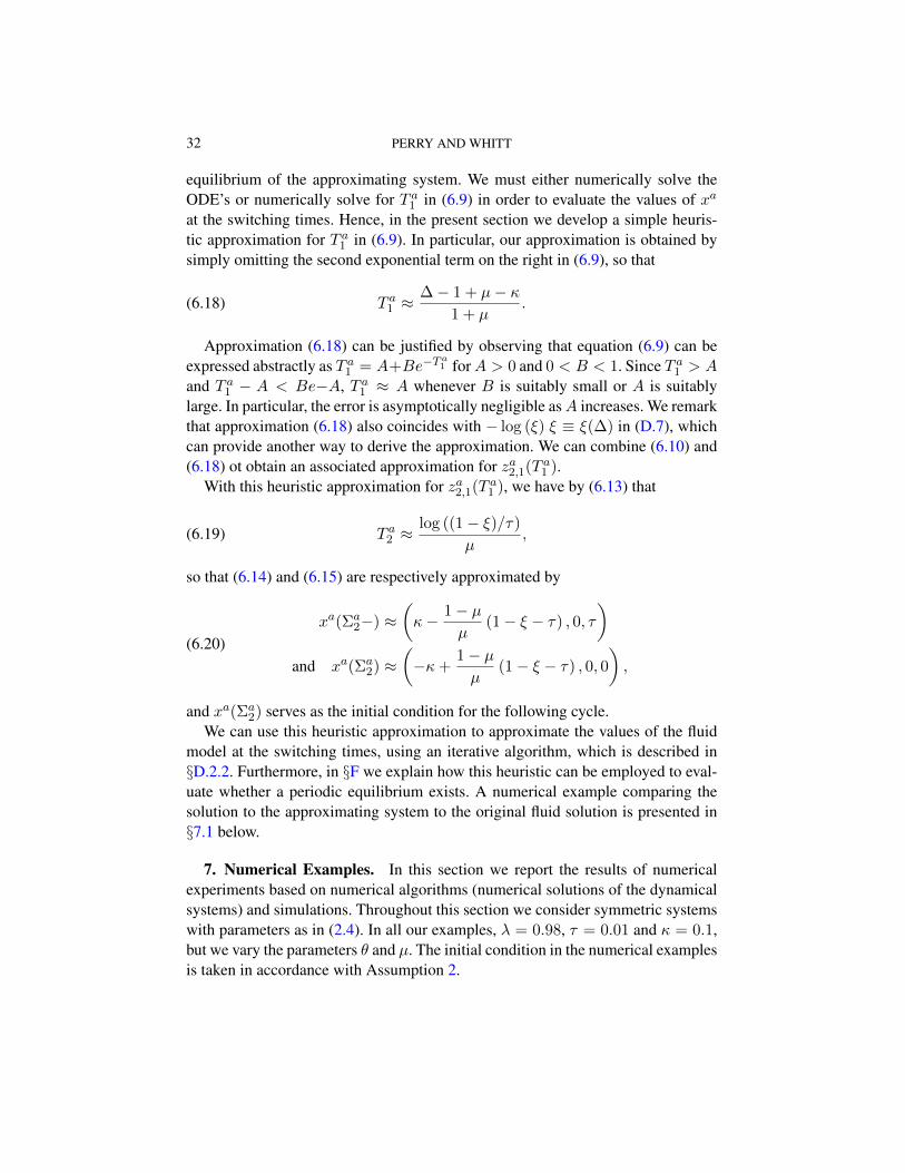
32 PERRY AND WHITT
equilibrium of the approximating system. We must either numerically solve theODE’s or numerically solve for T a1 in (6.9) in order to evaluate the values of xa
at the switching times. Hence, in the present section we develop a simple heuris-tic approximation for T a1 in (6.9). In particular, our approximation is obtained bysimply omitting the second exponential term on the right in (6.9), so that
(6.18) T a1 ≈∆− 1 + µ− κ
1 + µ.
Approximation (6.18) can be justified by observing that equation (6.9) can beexpressed abstractly as T a1 = A+Be−T
a1 forA > 0 and 0 < B < 1. Since T a1 > A
and T a1 − A < Be−A, T a1 ≈ A whenever B is suitably small or A is suitablylarge. In particular, the error is asymptotically negligible asA increases. We remarkthat approximation (6.18) also coincides with − log (ξ) ξ ≡ ξ(∆) in (D.7), whichcan provide another way to derive the approximation. We can combine (6.10) and(6.18) ot obtain an associated approximation for za2,1(T a1 ).
With this heuristic approximation for za2,1(T a1 ), we have by (6.13) that
(6.19) T a2 ≈log ((1− ξ)/τ)
µ,
so that (6.14) and (6.15) are respectively approximated by
xa(Σa2−) ≈
(κ− 1− µ
µ(1− ξ − τ) , 0, τ
)and xa(Σa
2) ≈(−κ+
1− µµ
(1− ξ − τ) , 0, 0
),
(6.20)
and xa(Σa2) serves as the initial condition for the following cycle.
We can use this heuristic approximation to approximate the values of the fluidmodel at the switching times, using an iterative algorithm, which is described in§D.2.2. Furthermore, in §F we explain how this heuristic can be employed to eval-uate whether a periodic equilibrium exists. A numerical example comparing thesolution to the approximating system to the original fluid solution is presented in§7.1 below.
7. Numerical Examples. In this section we report the results of numericalexperiments based on numerical algorithms (numerical solutions of the dynamicalsystems) and simulations. Throughout this section we consider symmetric systemswith parameters as in (2.4). In all our examples, λ = 0.98, τ = 0.01 and κ = 0.1,but we vary the parameters θ and µ. The initial condition in the numerical examplesis taken in accordance with Assumption 2.
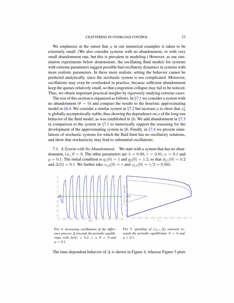
CHATTERING IN OVERLOAD CONTROL 33
We emphasize at the outset that µ in our numerical examples is taken to beextremely small. (We also consider systems with no abandonment, or with verysmall abandonment rate, but this is prevalent in modeling.) However, as our sim-ulation experiments below demonstrate, the oscillating fluid models for systemswith extreme parameters suggest possible bad oscillatory dynamics in systems withmore realistic parameters. In these more realistic setting the behavior cannot bepredicted analytically, since the stochastic system is too complicated. Moreover,oscillations may even be overlooked in practice, because sufficient abandonmentkeep the queues relatively small, so that congestion collapse may fail to be noticed.Thus, we obtain important practical insights by rigorously studying extreme cases.
The rest of this section is organized as follows. In §7.1 we consider a system withno abandonment (θ = 0) and compare the results to the heuristic approximatingmodel in §6.4. We consider a similar system in §7.2 but increase µ to show that x∗0is globally asymptotically stable, thus showing the dependence on µ of the long-runbehavior of the fluid model, as was established in §6. We add abandonment in §7.3in comparison to the system in §7.1 to numerically support the reasoning for thedevelopment of the approximating system in §6. Finally, in §7.4 we present simu-lations of stochastic systems for which the fluid limit has no oscillatory solutions,and show that stochasticity may lead to substantial oscillations.
7.1. A System with No Abandonment. We start with a system that has no aban-donment, i.e., θ = 0. The other parameters are λ = 0.98, τ = 0.01, κ = 0.1 andµ = 0.1. The initial condition is q1(0) = 1 and q2(0) = 1.2, so that d2,1(0) = 0.2and ∆(0) = 0.1. We further take z1,2(0) = τ and z2,1(0) = τ/2 = 0.005.
0 100 200 300 400 500 600 700 800 900 1000
−8
−6
−4
−2
0
2
4
6
8
Time
FIG 4. increasing oscillations of the differ-ence process ∆ towards the periodic equilib-rium, with ∆(0) = 0.2 > κ, θ = 0 andµ = 0.1.
0 0.1 0.2 0.3 0.4 0.5 0.6 0.7 0.8 0.9 1
−8
−6
−4
−2
0
2
4
6
8
z2,1
Diff
ere
nce process
FIG 5. spiraling of (z2,1,∆) outward to-wards the periodic equilibrium; θ = 0 andµ = 0.1.
The time-dependent behavior of ∆ is shown in Figure 4, whereas Figure 5 plots
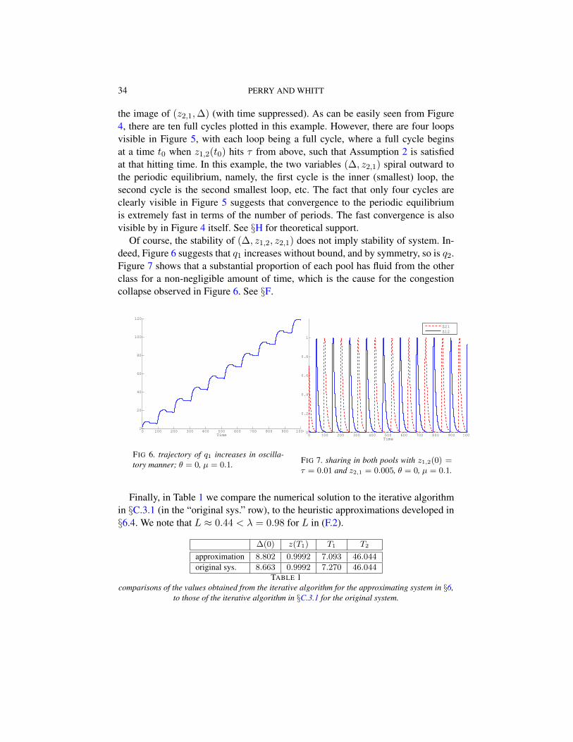
34 PERRY AND WHITT
the image of (z2,1,∆) (with time suppressed). As can be easily seen from Figure4, there are ten full cycles plotted in this example. However, there are four loopsvisible in Figure 5, with each loop being a full cycle, where a full cycle beginsat a time t0 when z1,2(t0) hits τ from above, such that Assumption 2 is satisfiedat that hitting time. In this example, the two variables (∆, z2,1) spiral outward tothe periodic equilibrium, namely, the first cycle is the inner (smallest) loop, thesecond cycle is the second smallest loop, etc. The fact that only four cycles areclearly visible in Figure 5 suggests that convergence to the periodic equilibriumis extremely fast in terms of the number of periods. The fast convergence is alsovisible by in Figure 4 itself. See §H for theoretical support.
Of course, the stability of (∆, z1,2, z2,1) does not imply stability of system. In-deed, Figure 6 suggests that q1 increases without bound, and by symmetry, so is q2.Figure 7 shows that a substantial proportion of each pool has fluid from the otherclass for a non-negligible amount of time, which is the cause for the congestioncollapse observed in Figure 6. See §F.
0 100 200 300 400 500 600 700 800 900 10000
20
40
60
80
100
120
Time
FIG 6. trajectory of q1 increases in oscilla-tory manner; θ = 0, µ = 0.1.
0 100 200 300 400 500 600 700 800 900 10000
0.2
0.4
0.6
0.8
1
Time
Z21Z12
FIG 7. sharing in both pools with z1,2(0) =τ = 0.01 and z2,1 = 0.005, θ = 0, µ = 0.1.
Finally, in Table 1 we compare the numerical solution to the iterative algorithmin §C.3.1 (in the “original sys.” row), to the heuristic approximations developed in§6.4. We note that L ≈ 0.44 < λ = 0.98 for L in (F.2).
∆(0) z(T1) T1 T2
approximation 8.802 0.9992 7.093 46.044
original sys. 8.663 0.9992 7.270 46.044TABLE 1
comparisons of the values obtained from the iterative algorithm for the approximating system in §6,to those of the iterative algorithm in §C.3.1 for the original system.
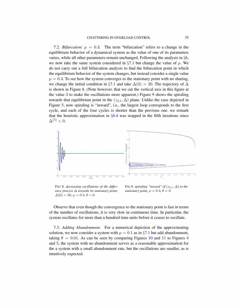
CHATTERING IN OVERLOAD CONTROL 35
7.2. Bifurcation: µ = 0.3. The term “bifurcation” refers to a change in theequilibrium behavior of a dynamical system as the value of one of its parametersvaries, while all other parameters remain unchanged. Following the analysis in §6,we now take the same system considered in §7.1 but change the value of µ. Wedo not carry out a full bifurcation analysis to find the bifurcation point in whichthe equilibrium behavior of the system changes, but instead consider a single valueµ = 0.3. To see how the system converges to the stationary point with no sharing,we change the initial condition in §7.1 and take ∆(0) = 20. The trajectory of ∆is shown in Figure 8. (Note however, that we cut the vertical axis in this figure atthe value 3 to make the oscillations more apparent.) Figure 9 shows the spiralingtowards that equilibrium point in the (z2,1,∆) plane. Unlike the case depicted inFigure 5, now spiraling is “inward”, i.e., the largest loop corresponds to the firstcycle, and each of the four cycles is shorter than the previous one. we remarkthat the heuristic approximation in §6.4 was stopped in the fifth iterations since∆(5) < 0.
0 100 200 300 400 500 600 700 800 900 1000−3
−2
−1
0
1
2
3
Time
FIG 8. decreasing oscillations of the differ-ence process ∆ towards its stationary point;∆(0) = 20, µ = 0.3, θ = 0.
0 0.1 0.2 0.3 0.4 0.5 0.6 0.7 0.8 0.9 1−5
0
5
10
15
20
z2,1
Diff
ere
nce Process
FIG 9. spiraling “inward” of (z2,1,∆) to thestationary point, µ = 0.3, θ = 0.
Observe that even though the convergence to the stationary point is fast in termsof the number of oscillations, it is very slow in continuous time. In particular, thesystem oscillates for more than a hundred time units before it ceases to oscillate.
7.3. Adding Abandonment. For a numerical depiction of the approximatingsolution, we now consider a system with µ = 0.1 as in §7.1 but add abandonment,taking θ = 0.01. As can be seen by comparing Figures 10 and 11 to Figures 4and 5, the system with no abandonment serves as a reasonable approximation forthe a system with a small abandonment rate, but the oscillations are smaller, as isintuitively expected.
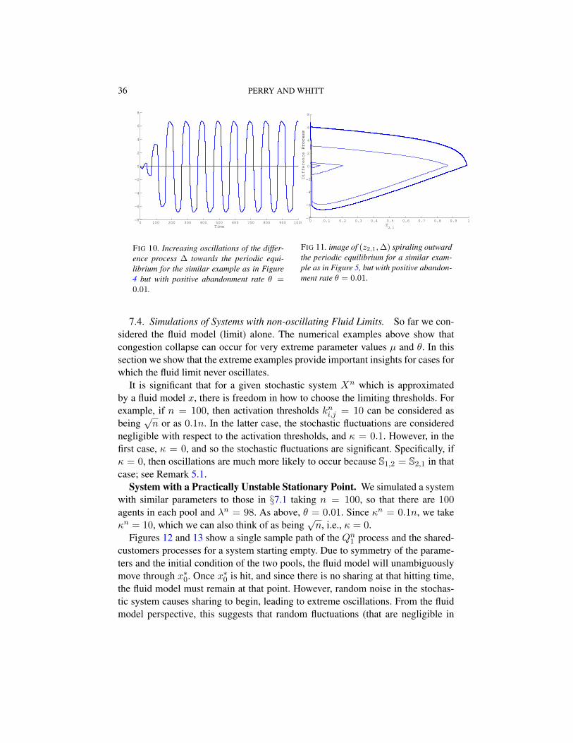
36 PERRY AND WHITT
0 100 200 300 400 500 600 700 800 900 1000−8
−6
−4
−2
0
2
4
6
8
Time
FIG 10. Increasing oscillations of the differ-ence process ∆ towards the periodic equi-librium for the similar example as in Figure4 but with positive abandonment rate θ =0.01.
0 0.1 0.2 0.3 0.4 0.5 0.6 0.7 0.8 0.9 1−8
−6
−4
−2
0
2
4
6
8
z2,1
Diff
ere
nce
Process
FIG 11. image of (z2,1,∆) spiraling outwardthe periodic equilibrium for a similar exam-ple as in Figure 5, but with positive abandon-ment rate θ = 0.01.
7.4. Simulations of Systems with non-oscillating Fluid Limits. So far we con-sidered the fluid model (limit) alone. The numerical examples above show thatcongestion collapse can occur for very extreme parameter values µ and θ. In thissection we show that the extreme examples provide important insights for cases forwhich the fluid limit never oscillates.
It is significant that for a given stochastic system Xn which is approximatedby a fluid model x, there is freedom in how to choose the limiting thresholds. Forexample, if n = 100, then activation thresholds kni,j = 10 can be considered asbeing
√n or as 0.1n. In the latter case, the stochastic fluctuations are considered
negligible with respect to the activation thresholds, and κ = 0.1. However, in thefirst case, κ = 0, and so the stochastic fluctuations are significant. Specifically, ifκ = 0, then oscillations are much more likely to occur because S1,2 = S2,1 in thatcase; see Remark 5.1.
System with a Practically Unstable Stationary Point. We simulated a systemwith similar parameters to those in §7.1 taking n = 100, so that there are 100agents in each pool and λn = 98. As above, θ = 0.01. Since κn = 0.1n, we takeκn = 10, which we can also think of as being
√n, i.e., κ = 0.
Figures 12 and 13 show a single sample path of the Qn1 process and the shared-customers processes for a system starting empty. Due to symmetry of the parame-ters and the initial condition of the two pools, the fluid model will unambiguouslymove through x∗0. Once x∗0 is hit, and since there is no sharing at that hitting time,the fluid model must remain at that point. However, random noise in the stochas-tic system causes sharing to begin, leading to extreme oscillations. From the fluidmodel perspective, this suggests that random fluctuations (that are negligible in

CHATTERING IN OVERLOAD CONTROL 37
fluid scale) quickly push the fluid limit from x∗0 to a state γ ∈ O, leading to fluid-scaled fluctuations.
0 50 100 150 200 250 300 350 400 450 5000
500
1000
1500
2000
2500
Time
FIG 12. simulated sample path of Qn1 ; n =100, λn = 98 κn = 10, θ = 0.01, µ = 0.1
0 50 100 150 200 250 300 350 400 450 5000
0.1
0.2
0.3
0.4
0.5
0.6
0.7
0.8
0.9
1
Time
Z2,1Z1,2
FIG 13. simulated sample path of the numberof shared customers in service in both pools;n = 100, λn = 98 κn = 10, θ = 0.01,µ = 0.1
System with no Oscillating Solutions (O = φ). The fluid model gives impor-tant insight that cannot be obtained analytically even for systems with O = φ, i.e.,systems that do not have oscillating fluid limits. We now taken = 100: λn = 98, µ = 0.5, θ = 0.5, τn = 1 and kni,j = 10,with the rest of the parameters being the same as in §7.1. The parameters θ andµ here are more likely in a practical call-center setting than the parameters in theexamples above.
To show that O = φ we solve the fluid model for an extreme example withq1(0) = 1 and q2(0) = 1000, z1,2 = τ and z2,1 = 0. In the simulation however,we have Zn2,1 = 20 and Zn1,2 = 0, which is a likely initial condition for a systemrecovering from an overload in queue 2. (The initial conditions of the stochasticsystem and the fluid model do not match because we want to show that the fluidmodel does not oscillate, and has no periodic equilibrium.)
Figure 14 shows a single sample path of the shared-customers processes from asingle simulation run, and Figure 15 shows the fluid model of the system with theinitial condition specified above. We only show figures of the shared customers ser-vice process, because both queues monotonically decrease to 0 in the fluid model,whereas customer abandonment make the oscillations of the queue processes unob-servable in the simulation. From the practical point of view, this means that oscilla-tions may be hard to detect in real time, unless one knows to look for them. Specif-ically, if the control parameters are chosen in accordance with the fluid model soas to ensure that the system will not oscillate, and if only the queues are observed,
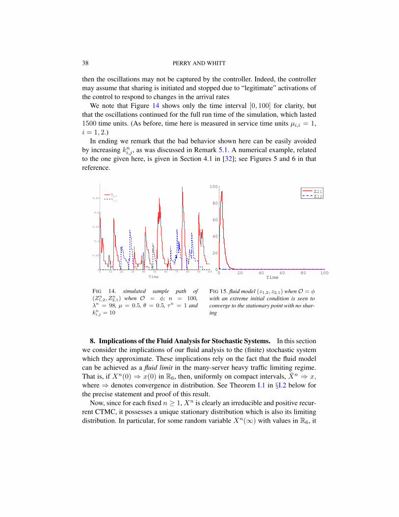
38 PERRY AND WHITT
then the oscillations may not be captured by the controller. Indeed, the controllermay assume that sharing is initiated and stopped due to “legitimate” activations ofthe control to respond to changes in the arrival rates
We note that Figure 14 shows only the time interval [0, 100] for clarity, butthat the oscillations continued for the full run time of the simulation, which lasted1500 time units. (As before, time here is measured in service time units µi,i = 1,i = 1, 2.)
In ending we remark that the bad behavior shown here can be easily avoidedby increasing kni,j , as was discussed in Remark 5.1. A numerical example, relatedto the one given here, is given in Section 4.1 in [32]; see Figures 5 and 6 in thatreference.
0 10 20 30 40 50 60 70 80 90 1000
0.05
0.1
0.15
0.2
0.25
Time
Z2,1
Z1,2
FIG 14. simulated sample path of(Zn1,2, Z
n2,1) when O = φ; n = 100,
λn = 98, µ = 0.5, θ = 0.5, τn = 1 andkni,j = 10
0 20 40 60 80 1000
20
40
60
80
100
Time
Z21Z12
FIG 15. fluid model (z1,2, z2,1) when O = φwith an extreme initial condition is seen toconverge to the stationary point with no shar-ing
8. Implications of the Fluid Analysis for Stochastic Systems. In this sectionwe consider the implications of our fluid analysis to the (finite) stochastic systemwhich they approximate. These implications rely on the fact that the fluid modelcan be achieved as a fluid limit in the many-server heavy traffic limiting regime.That is, if Xn(0) ⇒ x(0) in R6, then, uniformly on compact intervals, Xn ⇒ x,where ⇒ denotes convergence in distribution. See Theorem I.1 in §I.2 below forthe precise statement and proof of this result.
Now, since for each fixed n ≥ 1, Xn is clearly an irreducible and positive recur-rent CTMC, it possesses a unique stationary distribution which is also its limitingdistribution. In particular, for some random variable Xn(∞) with values in R6, it
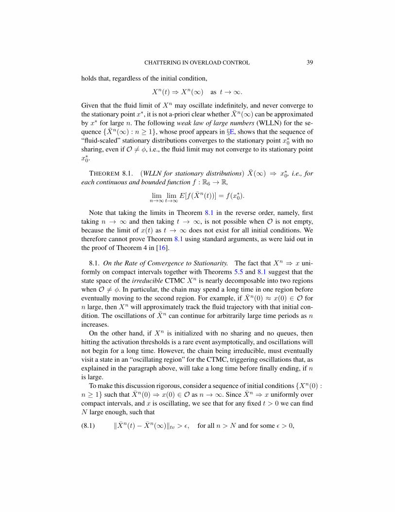
CHATTERING IN OVERLOAD CONTROL 39
holds that, regardless of the initial condition,
Xn(t)⇒ Xn(∞) as t→∞.
Given that the fluid limit of Xn may oscillate indefinitely, and never converge tothe stationary point x∗, it is not a-priori clear whether Xn(∞) can be approximatedby x∗ for large n. The following weak law of large numbers (WLLN) for the se-quence {Xn(∞) : n ≥ 1}, whose proof appears in §E, shows that the sequence of“fluid-scaled” stationary distributions converges to the stationary point x∗0 with nosharing, even if O 6= φ, i.e., the fluid limit may not converge to its stationary pointx∗0.
THEOREM 8.1. (WLLN for stationary distributions) X(∞) ⇒ x∗0, i.e., foreach continuous and bounded function f : R6 → R,
limn→∞
limt→∞
E[f(Xn(t))] = f(x∗0).
Note that taking the limits in Theorem 8.1 in the reverse order, namely, firsttaking n → ∞ and then taking t → ∞, is not possible when O is not empty,because the limit of x(t) as t → ∞ does not exist for all initial conditions. Wetherefore cannot prove Theorem 8.1 using standard arguments, as were laid out inthe proof of Theorem 4 in [16].
8.1. On the Rate of Convergence to Stationarity. The fact that Xn ⇒ x uni-formly on compact intervals together with Theorems 5.5 and 8.1 suggest that thestate space of the irreducible CTMC Xn is nearly decomposable into two regionswhen O 6= φ. In particular, the chain may spend a long time in one region beforeeventually moving to the second region. For example, if Xn(0) ≈ x(0) ∈ O forn large, then Xn will approximately track the fluid trajectory with that initial con-dition. The oscillations of Xn can continue for arbitrarily large time periods as nincreases.
On the other hand, if Xn is initialized with no sharing and no queues, thenhitting the activation thresholds is a rare event asymptotically, and oscillations willnot begin for a long time. However, the chain being irreducible, must eventuallyvisit a state in an “oscillating region” for the CTMC, triggering oscillations that, asexplained in the paragraph above, will take a long time before finally ending, if nis large.
To make this discussion rigorous, consider a sequence of initial conditions {Xn(0) :n ≥ 1} such that Xn(0) ⇒ x(0) ∈ O as n → ∞. Since Xn ⇒ x uniformly overcompact intervals, and x is oscillating, we see that for any fixed t > 0 we can findN large enough, such that
(8.1) ‖Xn(t)− Xn(∞)‖tv > ε, for all n > N and for some ε > 0,
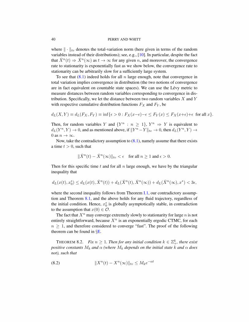
40 PERRY AND WHITT
where ‖ · ‖tv denotes the total-variation norm (here given in terms of the randomvariables instead of their distributions); see, e.g., [10]. In particular, despite the factthat Xn(t) ⇒ Xn(∞) as t → ∞ for any given n, and moreover, the convergencerate to stationarity is exponentially fast as we show below, the convergence rate tostationarity can be arbitrarily slow for a sufficiently large system.
To see that (8.1) indeed holds for all n large enough, note that convergence intotal variation implies convergence in distribution (the two notions of convergenceare in fact equivalent on countable state spaces). We can use the Levy metric tomeasure distances between random variables corresponding to convergence in dis-tribution. Specifically, we let the distance between two random variables X and Ywith respective cumulative distribution functions FX and FY , be
dL(X,Y ) ≡ dL(FX , FY ) ≡ inf{ε > 0 : FX(x−ε)−ε ≤ FY (x) ≤ FX(x+ε)+ε for all x}.
Then, for random variables Y and {Y n : n ≥ 1}, Y n ⇒ Y is equivalent todL(Y n, Y )→ 0, and as mentioned above, if ‖Y n−Y ‖tv → 0, then dL(Y n, Y )→0 as n→∞.
Now, take the contradictory assumption to (8.1), namely assume that there existsa time t > 0, such that
‖Xn(t)− Xn(∞)‖tv < ε for all n ≥ 1 and ε > 0.
Then for this specific time t and for all n large enough, we have by the triangularinequality that
dL(x(t), x∗0) ≤ dL(x(t), Xn(t)) + dL(Xn(t), Xn(∞)) + dL(Xn(∞), x∗) < 3ε,
where the second inequality follows from Theorem I.1, our contradictory assump-tion and Theorem 8.1, and the above holds for any fluid trajectory, regardless ofthe initial condition. Hence, x∗0 is globally asymptotically stable, in contradictionto the assumption that x(0) ∈ O.
The fact thatXn may converge extremely slowly to stationarity for large n is notentirely straightforward, because Xn is an exponentially ergodic CTMC, for eachn ≥ 1, and therefore considered to converge “fast”. The proof of the followingtheorem can be found in §E.
THEOREM 8.2. Fix n ≥ 1. Then for any initial condition k ∈ Z6+, there exist
positive constants Mk and α (where Mk depends on the initial state k and α doesnot), such that
(8.2) ‖Xn(t)−Xn(∞)‖tv ≤Mke−αt
CHATTERING IN OVERLOAD CONTROL 41
9. Important Takeaways for SSC-Inducing Controls. An SSC-inducing con-trol for a stochastic system is commonly designed in order to achieve an optimalcontrol for a diffusion approximation of the system. In particular, stochastic net-works can rarely be analyzed exactly, even under a fixed control, and finding a“good” control that is nearly optimal (in an appropriate sense), and is furthermoreimplementable, is a prohibitively hard problem. The most prevalent approach tosolving an optimal control problem, initiated by Harrison [17], is to solve a re-lated Diffusion Control Problem (DCP) for the system in heavy traffic, and thentranslate the optimal control for the DCP into a control for the system it approxi-mates. As reviewed in [7], a key step in this procedure is to formulate an equivalentworkload formulation (EWF), in which the dimension of the workload process isreduced. Thus, an optimal control for the approximating diffusion process foundvia the DCP scheme, dictates an SSC-inducing control for the stochastic system,which forces the asymptotic workload process to a lower-dimensional “boundary”subset of its state space. In fact, the FQR-ART control considered in this paper wasdeveloped by an analogous approach: In [28] we optimized a fluid model of thestochastic system, and then proposed a control to achieve the optimal fluid solu-tion.
Before describing general insights obtained from our analysis here, we mentionthat the FQR-ART control in the prelimit, and its limiting counterpart, share someof the general characteristics of SSC-inducing control and the resulting limitingcontrol. First note that an optimal control for an EWF is necessarily “bang-bang”with a singular part in the sense of [19], namely, such a control uses the maximum“pushing” towards the boundary set when the queue is away from it, and switchesinstantaneously between the directions of pushing to maintain the queue on theboundary. Similarly, the control process in both FQR-ART and the resulting lim-iting control use the maximum force to push the queues toward the threshold andthe boundary set, respectively. See also the paragraph below the display of S1,2 andS2,1 in §2.2, page 12.
We further observe that, in addition to the bang-bang portion, FQR-ART alsohas a “no-action” zone associated with states in which both difference processesare below the activation thresholds, or when one of the difference process is aboveits corresponding activation threshold, but the release threshold prevents the con-trol from being activated. Our analysis here revealed that the no-action zone isresponsible for the delayed activation of the control, and to the resulting oscilla-tions when the control parameters are not chosen correctly. In that regard, we makethe following general observation: While much attention had been given in the lit-erature to the difficulties in translating an optimal control for limiting approxima-tions (typically diffusion approximations) to a control for the underlying sequenceof stochastic systems, little attention was given to the difficulty in translating the
42 PERRY AND WHITT
asymptotic control parameters (when such a control is found) to a fixed system.Our analysis sheds light to possible problems that can arise in this second layer oftranslation. (Recall Remark 5.1 and the example in Figures 12-13. We discuss thisissue further in §J in the appendix.)
We next demonstrate with specific examples how our insights apply to othermodels.
9.1. A Comparison with the N model. To make the discussion concrete, wenow compare some conceptual similarities between our model and the N modelwhich was studied extensively in the single-server stations setting; see, e.g., [18,20] and [2]. We refer to these references for other works on the N model in theconventional heavy traffic, and to [45] for a many-server heavy-traffic study of anN system. (We further remark that the N model is covered by the model consideredin [15].)
The N model, depicted in Figure 3 above, has two single-server stations, with theserver in station 1 dedicated to serving class-1 jobs, while the server in station 2 canhandle both queues. (note that there are no arrows representing abandonment fromthe queues.) A (non-idling) service policy determines which queue server 2 shouldhandle when both queues are non empty. Similarly to our simulation experimentsin [28], which showed that the QIR control applied to a critically-loaded X systemcan lead to congestion collapse (see §2 above), a simulation in [18] demonstratedthat a naive implementation of the cµ rule, under which server 2 always prioritizesthe class 1 queue, may lead to congestion collapse in a critically-loaded N model.
A solution to a DCP for the N model led the authors in [2] to design a thresholdpolicy and prove that this policy is asymptotically optimal and leads to SSC. Underthat policy, server 2 helps queue 1 only when that queue is larger than a threshold,and otherwise this server only serves its own queue. It is further assumed that server2 preempts the job it processes if it needs to switch the class it serves. Note thatthis control uses the maximum force to push queue 1 towards the threshold, andhas a no-action zone associated with queue 1 being below that threshold. Since thethreshold is taken to be O(log n) as n → ∞, asymptotic SSC about the thresholdimplies that queue 1 is null in the diffusion limit. In particular, it is shown thatthe two-dimensional queue process has all its mass on the class-2 queue, and theidleness process has all its mass on server 2 (i.e., the class 1 queue is asymptoticallynull, and server 1 never idle). Observe that the no-action zone shrinks to 0 as nincreases, so that it does not appear in the limit.
It is significant that the asymptotics in [2] were achieved under the assumptionthat server 2 can switch in zero time between the two queues. This assumption isreasonable to make if the switching times in reality are sufficiently small relativeto the service time, but it is intuitively clear that even short switching times will
CHATTERING IN OVERLOAD CONTROL 43
lead to diffusion-scaled chattering of queue 1 about the threshold. In fact, sinceserver 2 switches infinitely-often between the two queues in the limit over anyfinite time interval, non-zero switching times may push the system to an overload,because switching times of server 2 essentially increase its idle period. Moreover,if the O(log n) threshold is not chosen appropriately for a given stochastic system,and in particular, if the the threshold is chosen to be too small, then, as in theexample in [18], server 2 will again spend too much time helping queue 1, leadingto congestion of its own queue.
Finally, the authors in [2] remark that a hysteresis control with two thresholdscan be employed to avoid chattering of the queue about the threshold (see the re-mark at the bottom of p. 621 in this reference). Under this modified control, onlyonce queue 1 crosses an upper threshold will server 2 switch to help this queue, andthat help is turned off only once the queue returns to the lower threshold. It is againintuitively clear that, if the thresholds are not chosen appropriately for the fixedsystem, namely, if the lower threshold is too small and the upper one is too large,then server 2 may end up spending too much time helping queue 1, leading queue2 to increase without bound in an oscillatory manner. Indeed, the two-thresholdscontrol increases the “no-action” zone, in turn, leading to increased delays in acti-vating the control.
10. Summary. In this paper we considered the FQR-ART overload controlapplied to the cyclic X model, when the control parameters are badly chosen. Forthe dynamical-system (fluid) limit, the purpose of the control is to attract any fluidtrajectory to one of two sliding manifolds during overload periods, so as to maintaina pre-specified ratio between the two queues.
Switching Fluid Limit. We have shown that possible delays in activation andrelease of the control can lead to chattering and resulting oscillations, which trans-lates to fluid-scaled fluctuations in the underlying stochastic system. The patho-logical oscillatory behavior can be analyzed via a switching dynamical system, asin Definition 3.1, within the framework of the many-server heavy-traffic FWLLN(Theorem I.1 in §I.2). Theorems 5.2 and 5.4, respectively, prove that the fluid limithas a unique stationary point and a non-trivial periodic equilibrium that is associ-ated with the oscillatory motion. Sufficient conditions for endless oscillations wereprovided in Theorem 5.5.
Fluid Stability. In Theorem 5.3 it was shown that any fluid trajectory that ceasesto oscillate must converge to the unique stationary point. A convenient approximat-ing dynamical system to the fluid limit was developed and shown to be bi-stablein §6. Specifically, all the trajectories of the approximating system were shown toconverge to one of the two equilibria – the stationary point x∗0 in (5.1), or a uniquenon-trivial periodic equilibrium. Finally, a simple heuristic construction in §6.4 can
44 PERRY AND WHITT
be used to approximate the values of the solutions to (3.10) at the switching times,and in particular, the values of the periodic equilibrium at the switching times,when it exists.
Implications. Numerical examples in §7 show the effectiveness of the approx-imating system. The simulation experiment in §7.4 demonstrates that our fluidmodel provides important insights into the untractable behavior of the underlyingstochastic system, even when the fluid approximation itself is not oscillating.
From the theoretical stochastic perspective, the results in §8 demonstrate that,despite the fact that the stochastic system is an ergodic CTMC, and is even expo-nentially ergodic by Theorem 8.2, an oscillatory behavior of the fluid model impliesthat it may take very long time for the system to converge to stationarity. In partic-ular, exponential ergodicity should does not necessarily imply “fast” convergenceto stationarity.
From the practical perspective, the most important conclusion is that the controlparameters must be chosen with caution. For example, the bad oscillatory behaviorpresented in §7.4 (which may be hard to detect in real time) can be avoided bychoosing appropriate activation thresholds. We again refer to [32] for a furtherdiscussion.
Acknowledgements. We thank Editor Assaf Zeevi for suggestions that led towriting Section 9. The first author received support from National Science Founda-tion (NSF) Grant CMMI 1436518. The second author received support from NSFGrants CMMI 1265070 and 1634133.
REFERENCES
[1] Asmussen, S. (2003). Applied probability and queues. Springer.[2] Bell, S. L. and Williams, R.J. (2001). Dynamic scheduling of a system with two parallel servers
in heavy traffic with resource pooling: asymptotic optimality of a threshold policy. The Annalsof Applied Probability, 11 (3) 608–649.
[3] Billah, K. Y. and Scanlan, R. H. (1991). Resonance, Tacoma Narrows bridge failure, and un-dergraduate physics textbooks, American Journal of Physics, 59 (2), 118–124.
[4] Bramson, M. (1998). State space collapse with application to heavy traffic limits for multiclassqueueing networks. Queueing Systems, 30, (1-2), 89–140.
[5] Bramson, M. (1994). Instability of FIFO queueing networks. The Annals of Applied Probability4 (2), 414–431.
[6] Bramson, M. (2008). Stability of queueing networks. Springer.[7] Bramson, M. and Williams, R. J. (2000). On dynamic scheduling of stochastic networks in
heavy traffic and some new results for the workload process Proceedings of the 39th IEEEConference on Decisions and Control, 516–521.
[8] Chase, C., Serrano, J., Ramadge, P. J. (1993). Periodicity and chaos from switched flow sys-tems: contrasting examples of discretely controlled continuous systems. IEEE Transactions onAutomatic Control 38 (1), 70–83.
CHATTERING IN OVERLOAD CONTROL 45
[9] Dai, J. G. (1995). On positive Harris recurrence of multiclass queueing networks: a unifiedapproach via fluid limit models. The Annals of Applied Probability 5 (1) 49–77.
[10] Durrett, R. (1991). Probability: theory and examples. Wadsworth and Brooks/Cole, PacificGrove, California.
[11] Erramilli, A. and Forys, L. J. (1991). Oscillations and chaos in a flow model of a switchingsystem. IEEE Journal on Selected Areas in Communications, 9 (2), 171–178.
[12] Filippov, A. F. (1988) Differential Equations with Discontinuous Righthand Sides. Kluwer Aca-demic Publishers, the Netherlands.
[13] Garnett, O., Mandelbaum, A. and Reiman, M. (2002). Designing a call center with impatientcustomers, Manufacturing & Service Operations Management, 4, (3), 208–227.
[14] Gurvich, I. and Whitt, W. (2009). Scheduling Flexible Servers with Convex Delay Costs inMany-Server Service Systems. Manufacturing & Service Operations Management, 11 (2), 237-253.
[15] Gurvich, I. and Whitt, W. (2009). Queue-and-Idleness-Ratio Controls in Many-Server ServiceSystems. Mathematics of Operations Research 34 (2), 363–396.
[16] Halfin, S. and Whitt, W. (1981). Heavy-traffic limits for queues with many exponential servers.Operations Research 29 (3) 567–588.
[17] Harrison, J. M. (1988). Brownian models of queueing networks with heterogeneous customerpopulations Stochastic differential systems, stochastic control theory and applications, 147–186.
[18] Harrison, J.M. (1998). Heavy traffic analysis of a system with parallel servers: asymptoticoptimality of discrete-review policies. Annals of applied probability 8 (3) 822–848.
[19] Harrison, J. M. and Taskar, M. I. (1983). Instantaneous control of Brownian motion. Mathe-matics of Operations research, 8 (3) 439–453.
[20] Harrison, J. M. and Williams, R. J. (2005). Workload reduction of a generalized Browniannetwork. The Annals of Applied Probability, 15 (4), 2255–2295.
[21] Khalil, H. K. (2002). Nonlinear Systems. Prentice Hall, New Jersey.[22] Kontoyiannis I. and S.P. Meyn. (2003). Spectral Theory and Limit Theorems for Geometrically
Ergodic Markov Processes. The Annals of Applied Probability, Vol. 13, 304–362.[23] Liberzon, D. (2003). Switching in Systems and Control. Birkhauser, Boston.[24] Liu, Y. and Whitt, W. (2011). Nearly Periodic Behavior in the The Overloaded G/D/S +GI
Queue. Stochastic Systems, 1 (2), 340–410.[25] Lu S.H., Kumar P.R. (1991). Distributed scheduling based on due dates and buffer priorities.
IEEE Trans. Automat. Control.36(12), 1406–1416.[26] Matveev, A. S., Savkin, A. V. (2000). Qualitative theory of hybrid dynamical systems.
Birkhauser, Boston.[27] Pang, G., Talreja, R., Whitt, W., (2007). Martingale proofs of many-server heavy-traffic limits
for Markovian queues. Probability Surveys, 4, 193–267.[28] Perry, O., W. Whitt. (2009). Responding to unexpected overloads in large-scale service systems.
Management Sci., 55 (8), 1353–1367.[29] Perry, O., W. Whitt. (2011a). A fluid approximation for service systems responding to unex-
pected overloads. Oper. Res., 59 (5), 1159–1170.[30] Perry, O., W. Whitt. (2011b). An ODE for an overloaded X model involving a stochastic aver-
aging principle. Stochastic Systems, 1 (1), 17–66.[31] Perry, O., W. Whitt. (2013). A fluid limit for an overloaded X model via an averaging principle.
Math, Oper. Res., 38 (2), 294–349.
46 PERRY AND WHITT
[32] Perry, O., W. Whitt. (2015a). Achieving rapid recovery in an overload control for large-scaleservice systems. Forthcoming in INFORMS Journal on Computing.Available at: http://www.columbia.edu/∼ww2040/allpapers.html
[33] Perry, O., W. Whitt. (2015b). Online Supplement to Achieving rapid recovery in an over-load control for large-scale service systems. Forthcoming in INFORMS Journal on Computing.Available at: http://www.columbia.edu/∼ww2040/allpapers.html
[34] Reiman, M. I. (1984). Some diffusion approximations with state space collapse in Modellingand performance evaluation methodology. 207–240, Springer.
[35] Robert, P. (2003). Stochastic networks and queues, Springer-Verlag.[36] Rudin, W. (1991). Functional Analysis, McGraw-Hill, Inc., New York.[37] Rybko A.N., Stolyar A.L. (1992). Ergodicity of stochastic processes describing the operations
of open queueing networks. Problems Inform. Transmission 28, 3–26 (in Russian).[38] Sastry, S.S. and Desoer, C. A. (1981). Jump behavior of circuits and systems. IEEE Transac-
tions on Circuits and Systems 28 (12) 1109–1124.[39] Shah, D., D. Wischik. (2011). Fluid models of congestion collapse in overloaded switched
networks. Queueing Systems 69 121–143.[40] Schaft, V.D. and Schumacher, H. (2000). An introduction to hybrid dynamical systems Springer
Lecture Notes in Control and Information Sciences, Vol. 251. Springer-Verlag, London.[41] Shakkottai, S, R. Srikant, A. L. Stolyar. (2004). Pathwise optimality of the exponential schedul-
ing rule for wireless channels. Adv. Appl. Prob. 36 1021–1045.[42] Stewart, D.E. (2000). Rigid-body dynamics with friction and impact. SIAM review 42 (1) 3–39.[43] Stolyar, A. L. (2004). Maxweight scheduling in a generalized switch: state space collapse and
workload minimization in heavy traffic. Ann. Appl. Prob. 14 (1) 1–53.[44] Teschl, G. (2009). Ordinary Differential Equations and Dynamical Systems, Universitat Wien.
Available online: www.mat.univie.ac.at/∼gerald/ftp/book-ode/ode.pdf[45] Tezcan, T. and Dai, J. G. (2010). Dynamic control of N-systems with many servers: Asymptotic
optimality of a static priority policy in heavy traffic. Operations Research, 58 (1) 94–110.[46] Whitt, W. (1971). Weak Convergence Theorems for Priority Queues: Preemptive-Resume Dis-
cipline. Journal of Applied Probability 8 (1) 74–94.[47] Whitt, W. (1981). Comparing counting processes and queues. Adv. Appl. Prob. 13 (1) 207–220.[48] Whitt, W. (2002). Stochastic-Process Limits, New York, Springer.[49] Williams, R. J. (1998). Diffusion approximations for open multiclass queueing networks: suf-
ficient conditions involving state space collapse. Queueing systems 30 (1-2) 27–88.
APPENDIX A: OVERVIEW
This appendix contains supplementary material for the main paper. First, in §Bwe give notation for sets used in the paper, as well as sets that are used in the ap-pendix. The proofs of the results in Section §5 appear in §C, and the proofs of theresults in §6 are presented in §D. Both §§C and D include supporting results withtheir proofs, and efficient algorithms to compute the respective ODE’s in switchingtimes. The proofs of the theorems in §8 appear in §E. In §F we show how the ap-proximating system can be employed to check whether congestion collapse occurs,and in §G we present an algorithm to compute the solution to the heuristic approx-imation suggested in §6.4. In §H we establish stronger forms of convergence of
CHATTERING IN OVERLOAD CONTROL 47
solutions to the approximating system to their equilibrium behavior. In §I we showthat the fluid model we considered in the main paper arises as the fluid limit ina many-server heavy-traffic fluid limit of the underlying model. The proof of theFWLLN is given in §I.2, after a brief expansion on the stochastic model and many-server scaling in §I.1. Finally, in §J we discuss implications of our results here forthe control of the stochastic system.
APPENDIX B: NOTATION OF SETS
Below is a list of the different sets that appear in the paper. Their first appearanceis in parenthesis.
• S∗ – the set of all stationary points (§5.1).• M – switching (or sliding) manifold in a general system (§1).• O – the invariant set of oscillating solution, i.e., if x(0) ∈ O, then x oscillates
indefinitely (§5.1).• Pu∗ – the image of the periodic equilibrium u∗ (§4).• S ≡ [0, λ/θ]2 × [0, 1]4 – the state space of the fluid model (§2.2).• Si,j – the sliding manifold where di,j = κ (§2.2)• Su∗ – the stability region of the periodic equilibrium u∗ (§4).• Sx∗ – the stability region of a stationary point x∗ (§5.1).• Sx∗0 – the stability region of the stationary point x∗0 in (5.1) (Theorem 5.2).• Sa ≡ [0,∞)2 × [0, 1]4 – the state space of the approximating system (§6).• Sε ≡ [ε, λ/θ]2 × [0, τ ], ε > 0 – the state space of of solutions in O (§C.3.2).• Sκ ≡ [κ+εκ, λ/θ]×[0, τ ], where εκ > 0 (Proof of existence part of Theorem
5.4 in §C.3.3).• Sµ ≡ [∆M
µ − δµ,∆Mµ ], where ∆M
µ is defined in (D.2) and δµ in (D.8) (Equa-tion (D.5) in §D.2.3).
APPENDIX C: PROOF OF THE RESULTS IN SECTION 5
In this section we provide the proofs of the results in §5.
C.1. Proofs of Theorems 5.1, 5.2 and 5.3.
PROOF OF THEOREM 5.1. No sharing will ever occur because qi = (yi − 1)+,and if yi(t) > 1, so that the queue is positive, then yi(t) is decreasing at t, i = 1, 2.(Recall that λ < µ = 1.) Hence, even if di,j(0) = κ for (i, j) = (1, 2) or (i, j) =(2, 1), then di,j(t) < κ for any t > 0 in some right-neighborhood of 0. It followsthat, if zi,j(0) > 0, i 6= j, then zi,j is strictly decreasing, which implies that theservice capacity in pool j is increasing. In turn, qj must keep decreasing as longas it is strictly positive. Finally, since yi is strictly decreasing as long as it is larger
48 PERRY AND WHITT
than λ and is strictly increasing otherwise, we have
(C.1) yi(t)→ λ as t→∞.
PROOF OF THEOREM 5.2. Suppose that γ∗ = (γ∗i , γ∗i,j ; i, j = 1, 2) ∈ S∗, is
such that γ∗ ∈ S1,2 ∪ S+1,2, so that γ∗1 ≥ κ. Consider the fluid model initialized
at γ∗, i.e., x(0) = γ∗. If z2,1(0) = γ∗2,1 > 0, then by the rules of FQR-ART,z2,1(0) = −µ2,1z2,1(0) < 0, implying that z2,1 is strictly decreasing. It followsthat γ∗2,1 = 0, so that γ∗1,1 = 1 (because γ∗1 ≥ κ > 0). But then
q1(0) = λ− µ1,1γ∗1,1 − θq1(0) < λ− 1 < 0,
which contradicts the supposition that γ∗ is a stationary point. Hence, S∗ ∩ (S1,2 ∪S+
1,2) = φ. Similar arguments apply to S∗ ∩ (S2,1 ∪ S+2,1). The same reasoning
for γ∗ ∈ S∗ ∩ S−1,2 ∩ S−2,1 implies that γ∗1,2 = γ∗2,1 = 0 and γ∗1 = γ∗2 = 0.Then the arguments leading to (C.1) show that γ∗ = x∗0. Hence, we conclude thatS∗ = {x∗0}.
PROOF OF THEOREM 5.3. Since x(0) ∈ Oc there exists a time t0 ≥ 0 suchthat x(t) /∈ S+
1,2 ∪ S+2,1 for all t ≥ t0. If x(t) ∈ S−i,j for all t ≥ t0, then
zi,j(t) = −µzi,j(t), so that zi,j(t) = zi,j(t0)e−µ(t−t0), t ≥ t0.
Then both z1,2 and z2,1 converge to 0, and it is easy to see from (2.3) (recall thatthere is no new sharing taking place) that both queues will reach 0 in finite time.Then, after qi reaches 0, all arriving fluid moves immediately into service, so thatz2,2 = λ− z2,2, and we see that z2,2(t)→ λ as t→∞.
Now suppose that x ∈ S1,2 over an interval I . If z2,1 > τ over I , then no fluidflows from q1 to pool 2, so that both queues evolve independently according to(2.3). Since z1,2 and z2,1 are strictly decreasing over I , the same arguments givenabove apply in this case. Therefore, assume that z2,1 ≤ τ over an interval J ⊆ Iso that sharing is allowed. By Assumption 1, q1 is strictly decreasing on J , and thesliding motion implies that q1(t) − q2(t) = 0, so that q2 is strictly decreasing aswell (at exactly the same rate as q1). Now, some of the service capacity of pool 2is given to queue-1 fluid at any point, so that, for t ∈ J ,
q1(t) < λ−z1,1(t)−µz2,1(t)−θq1(t) and q2(t) > λ−z2,2(t)−µz1,2(t)−θq2(t).
Recalling that q1(t) = q2(t) + κ and zi,i(t) = 1− zj,i(t) for t ∈ J , we have
0 = q1(t)− q2(t) < (1− µ)(z2,1(t)− z1,2(t))− θκ < (1− µ)(z2,1(t)− z1,2(t)),

CHATTERING IN OVERLOAD CONTROL 49
so that z1,2(t) < z2,1(t). It follows that z1,2(t) ≤ τ and is decreasing on J . Inparticular, both queues continue decreasing after the sliding motion is over.
The same arguments give that, if x ever slides on S2,1, then both queues arestrictly increasing to 0. Hence, the processes z1,2 and z2,1 never increase above τduring sliding motion, so that both queues are strictly decreasing to 0. After qi hits0, zj,i decreases monotonically to 0 and zi,i converges to λ.
C.2. Bounds to Guarantee Oscillations. We now provide auxiliary results,needed for the proof of Theorem 5.5, providing sufficient conditions for endlessoscillations of solutions to (3.10) and congestion collapse. In §§C.2.1 and C.2.2we construct simple bounds on T1 and x(T1), and bounds on T2 and the values ofx over [Σ1,Σ2), respectively. Universal bounds on the solution x and the holdingtimes, and a numerical example, are given in §C.2.3.
C.2.1. Auxiliary Results: Bounds on T1 and x(T1). We can apply (3.16) toobtain bounds on T1.
COROLLARY C.1. (bounds on T1) Under the initial conditions in Assumption2, the interval end time T1 is bounded above and below by
(C.2) 0 <θκ+ ΨL
θ∆(0) + ΨL≤ e−θT1 ≤ θκ+ ΨU
θ∆(0) + ΨU< 1,
for ΨL and ΨU in (3.14), from which we deduce that
1 <θ∆(0) + ΨU
θκ+ ΨU≤ eθT1 ≤ θ∆(0) + ΨL
θκ+ ΨL<∞,
and
0 < log
(θ∆(0) + ΨU
θκ+ ΨU
)≤ θT1 ≤ log
(θ∆(0) + ΨL
θκ+ ΨL
)<∞.
The associated bounds on T1, denoted by TL1 ≡ TL1 (∆(0)) and TU1 ≡ TU1 (∆(0)),are both strictly increasing functions of ∆(0), both approaching 0 as ∆(0) ↓ κ and∞ as ∆(0) ↑ ∞. In particular,
TL1 ≡(
1
θ
)log
(θ∆(0) + ΨU
θκ+ ΨU
)=
(1
θ
)log
(1 +
∆(0)− κ(ΨU/θ) + κ
)≤ ∆(0)− κ
ΨU + θκ
and
TU1 ≡(
1
θ
)log
(θ∆(0) + ΨL
θκ+ ΨL
)=
(1
θ
)log
(1 +
∆(0)− κ(ΨL/θ) + κ
)≤ ∆(0)− κ
ΨL + θκ
50 PERRY AND WHITT
so that
0 < TU1 − TL1 =
(1
θ
)(log
(1 +
∆(0)− κ(ΨL/θ) + κ
)− log
(1 +
∆(0)− κ(ΨU/θ) + κ
))=
(1
θ
)(log
(θ∆(0) + ΨL
θκ+ ΨL
)(θκ+ ΨU
θ∆(0) + ΨU
)).
PROOF. Exploit (3.16) with the equation ∆(T1) = κ characterizing T1.
The bounds we have just obtained on T1 can be used to obtain bounds on q1(T1).Recall that κ < ∆(0) and ΨL < ΨU < 0. Applying (C.2) with (3.6), we immedi-ately obtain
COROLLARY C.2. (bounds on q1(T1)) q1(t) is bounded from below by qL1 andfrom above by qU1 , where, for ΨL and ΨU in (3.14),
0 < qL1 (T1) ≡ λ
θ−(λ
θ− q1(0)
)(θκ+ ΨL
θ∆(0) + ΨL
)≤ q1(T1) ≤ λ
θ−(λ
θ− q1(0)
)(θκ+ ΨU
θ∆(0) + ΨU
)≡ qU1 (T1) <∞.
Similarly, Applying (3.4), we have
COROLLARY C.3. (bounds on z2,1(T1))
0 < zL2,1(T1)) ≡ 1− e−T1 < z2,1(T1)) < 1− (1− τ)e−T1 ≡ zU2,1(T1)) < 1.
C.2.2. Bounds on T2 and {x(t) : T1 ≤ t ≤ T1 + T2). For bad oscillatorybehavior, we will want to see that q2(T1 + t) remains positive and, furthermore thatd2,1 < 0. to ensure that the initial conditions in Assumption 2 hold at the switchingtime Σ2 ≡ T1 + T2 with the index labels reversed. From Corollary C.2, we obtainthe following
COROLLARY C.4. (lower bounds on the queue lengths on [T1, T1 + T2))
q2(T1)− κ = q1(T1) ≥ qL1 (T1) =λ
θ−(λ
θ− q1(0)
)(θκ+ 2
θ∆(0) + 2
),
so that, for i = 1, 2,
qi(T1 + t) ≥ qL1 (T1)e−θt −(
1− λθ
)(1− e−θt)
=
(λ
θ−(λ
θ− q1(0)
)(κ+ 2
∆(0) + 2
))e−θt −
(1− λθ
)(1− e−θt),
CHATTERING IN OVERLOAD CONTROL 51
which is a strictly decreasing function of t. As a consequence, a sufficient conditionfor both q1(t) and q2(t) to remain positive throughout [T1, T1 + T2] is for(
λ
θ−(λ
θ− q1(0)
)(θκ+ 2
θ∆(0) + 2
))e−θT2 >
(1− λθ
)(1− e−θT2),
for which a sufficient condition is(λ
θ−(λ
θ− q1(0)
)(θκ+ 2
θ∆(0) + 2
))e−θT
U2 >
(1− λθ
)(1− e−θTU2 ),
where
TU2 ≡loge ([1− (1− z2,1(0))e−T
U1 ]/τ)
µ≤ loge ([1− (1− τ)e−T
U1 ]/τ)
µ.
for TU1 in Corollary C.1.
C.2.3. Universal Bounds. We now consider the performance over a range ofinitial conditions. First, we introduce lower and upper bounds on the initial differ-ence ∆(0) ≡ q2(0)− q1(0). We assume that
(C.3) 0 < κ < ∆L(0) ≤ ∆(0) ≤ ∆U (0) <∞
uniformly enforcing Assumption 2. We also assume that the smaller queue lengthis bounded below and above by
(C.4) 0 < qL1 (0) ≤ q1(0) ≤ qU1 (0) <λ
θ<∞,
again uniformly enforcing Assumption 2.Now let TL∗1 be the lower bound TL1 for T1 in Corollary C.1 when ∆(0) =
∆L(0) and let TU∗1 be the lower bound TU1 for T1 in Corollary C.1 when ∆(0) =∆U (0).
LEMMA C.1. (universal bounds on T1) For all initial conditions satisfying(C.3) and (C.4),
0 < TL∗1 ≤ T1 ≤ TU∗1 <∞.
PROOF. Apply Corollary C.1.
LEMMA C.2. (universal bounds on z2,1(T1) and T2) If, together with (C.3)and (C.4),
(C.5) 1− e−TL∗1 > τ,
52 PERRY AND WHITT
then1− e−T1 > τ, τ < z2,1(TL∗1 ) ≤ z2,1(T1) ≤ z2,1(TU∗1 )
and
(C.6) TL∗2 ≡ loge (z2,1(TL∗1 )/τ)
µ≤ T2 ≤
loge (z2,1(TU∗1 )/τ)
µ≡ TU∗2
for all initial conditions satisfying (C.3) and (C.4).
PROOF. Apply (3.4) and (3.21) together with Lemma C.2.
If a periodic equilibrium exists, then the value of z1,2(Σ2) will equal to z2,1(σ2)on that equilibrium, as explained below (3.2) in §3. See also (5.2) in Theorem 5.4.We put the results above together to obtain bounds on z1,2(T1 + T2), which willserve as the new value of z2,1(0) in a continuation of the algorithm beyond timeΣ2 = T1 + T2.
LEMMA C.3. (universal bounds on z1,2(Σ2) If conditions (C.3), (C.4) and(C.5) hold, then
0 < zL∗1,2(T1+T2) ≡ e−µTU∗1 z2,1(TU∗1 ) ≤ z1,2(T1+T2) ≤ e−µTL∗1 z2,1(TL∗1 ) ≡ zU∗1,2(T1+T2) < τ
for all initial conditions satisfying (C.3) and (C.4).
PROOF. Apply (3.22) together with the lemmas above.
Next we consider the queue lengths at time T1 + T2.
LEMMA C.4. (universal lower bounds on the queue lengths at time T1 + T2)If (C.3), (C.4) and (C.5) hold, then
q2(T1)− κ = q1(T1) ≥ qL∗1 (T1) ≡ λ
θ−(λ
θ− qL1 (0)
)(θκ+ 2
θ∆L(0) + 2
),
for all initial conditions satisfying (C.3) and (C.4), where qL1 (0) and ∆L(0) aregiven in (C.3) and (C.4). If, in addition,
(C.7) qL∗1 (T1 + T2) ≡ qL∗1 (T1)e−θTU∗2 >
(1− λθ
)(1− e−θTU∗2 ),
then the two queue lengths q1(t) and q2(t) remain positive throughout [T1, T1 +T2]for all initial conditions satisfying (C.3) and (C.4).
PROOF. Apply Corollary C.4 and (C.6).
CHATTERING IN OVERLOAD CONTROL 53
Finally, we obtain lower and upper bounds on the queue difference at time T1 +T2.
LEMMA C.5. (universal bounds on the queue difference at time T1 + T2) Ifconditions (C.3), (C.4) and (C.5) hold, then
∆L(T1 + T2) ≡ κe−θTU∗2 −AU
(e−θT
L∗2 − e−µTU∗2
µ− θ
)
≤ ∆(T1 + T2) ≤ ∆U (T1 + T2) ≡ κe−θTL∗2 −AL
(e−θT
U∗2 − e−µTLU∗2
µ− θ
)for all initial conditions satisfying (C.3) and (C.4), where TL∗2 and TU∗2 are givenin (C.6) and
AL ≡ (1− µ)(zL∗1,2(T1)− zU∗2,1(T1)) ≤ A ≤ (1− µ)(zU∗1,2(T1)− zL∗2,1(T1)) ≡ AU
for A in (3.18).
A Numerical Example.. Consider the bounds in Lemma C.5. Since κ is taken tobe relatively small,
∆L(T1 + T2) ≈ AU
(e−θT
L∗2 − e−µTU∗2
µ− θ
).
In addition, AU ≤ (1 − µ)(τ − 1), so that, for given µ and τ , A in this lemmais bounded from above by a constant. These observations help to determine aninitial value ∆L(0) for which (C.14) will be satisfied. For the same parameters in§7 µ = 0.1, λ = 0.98, τ = 0.01, κ = 0.1 and θ = 0.01, the constant bound ofAU is −0.891 and ∆L(T1 + T2) ≥ 6.21. Hence, (C.14) holds for some values of∆(0) in the interval (κ, 6.21). For example, taking ∆L(0) = 4, ∆U (0) = 7 andqL1 (0) = 1, we obtain ∆L(Σ1) ≈ 6 > ∆L(0) and qL1 (Σ1) = 1.8 > qL1 (0).
C.3. Proofs of Theorems 5.4 and 5.5. To establish these results, we exploit analgorithm for efficiently computing a solution to the switching model in (3.10) andefficiently calculating the periodic equilibrium if it exists. The algorithm improveson the piecewise numerical solution of the piecewise ODE in (3.10) by exploitingthe exact formulas in §3. We can recursively calculate the values at the switchingtimes Σi and then afterwards calculate the trajectory in between. By iterating, wecan easily determine numerically if the solution converges to the stationary point ornot. Numerical experience indicates that if the solution oscillates indefinitely, thenit rapidly converges to a periodic equilibrium. In particular, the algorithm identifiesthe periodic equilibrium. However, more is required to provide a mathematicalproof of existence, uniqueness and convergence.
54 PERRY AND WHITT
C.3.1. An Efficient Algorithm for The Periodic Equilibrium. A periodic equi-librium u∗ has an important closure property: If u∗(t) satisfies Assumption 2 forsome t, then u∗(t+ Σ4) = u∗(t). Due to the symmetry of our model, we can relatethe system state at time t+Σ2 to the system state at time t. The state at time t+Σ2
should coincide with the state at time t with the labels reversed. That is, we shouldhave
q1(t+ Σ2) = q2(t) > 0, q2(t+ Σ2) = q1(t) > 0
z1,2(t+ Σ2) = z2,1(t) and z2,1(t+ Σ2) = z1,2(t) = τ.(C.8)
with the condition that the pools remain full throughout:
z1,1(s) + z2,1(s) = 1 and z2,2(s) + z1,2(s) = 1, 0 ≤ s ≤ t+ Σ2.
(Observe that the labels of the processes in the second equality in (5.2) are re-versed.) If indeed we can establish the closure property in (C.8), then we will haveproved that there exists a periodic equilibrium.
It is natural to search for the equilibrium by iterating: We pick a candidate initialvector x3(0) ≡ (q1(0), q2(0), z2,1(0)), letting z1,2(0) = τ , so that Assumption 2holds. We then solve for T1, T2, and (q1(T1 + T2), q2(T1 + T2), z1,2(T1 + T2)), asindicated above. we then redefine (q1(0), q2(0), z2,1(0)) to be (q2(T1+T2), q1(T1+T2), z1,2(T1 + T2)) and repeat the calculation.
If at some iteration we obtain an unreasonable value for x3, e.g., qi < 0, i = 1or i = 2, or ∆ ≤ κ, then the algorithm is stopped and we conclude that the solutioncorresponding to the initial condition we chose converges to x∗0 (due to Theorem5.3). However, a pathological case has ∆ > κ for all iterations, but ∆ → κ. Let∆∗ and T ∗1 denote the limit of ∆ and T1 when the algorithm is iterated indefinitely.Observe that ∆∗ = κ implies T ∗1 = 0, so that the corresponding limiting solutionu∗ is necessarily a constant function. This case is clearly a pathology, due to theuniqueness of the stationary point x∗0. The following lemma ensures that such apathological behavior of the algorithm is not possible. In particular, if at someiteration of the algorithm ∆ is too close to κ, then this is also the last iteration.
LEMMA C.6. There exists εκ > 0 such that, if κ < ∆(0) < κ + εκ, thenx(Σ2) > −κ. In particular x(0) ∈ Oc, so that x(t)→ x∗0 as t→∞.
PROOF. By Lemma 3.1, ∆ is bounded from above by the linear function −ΨL.Hence, for any δ1 > 0 we can find ε1 > 0 such that, if κ < ∆(0) < κ + ε1,then 0 < T1 < δ1. The explicit expressions of z2,1 in (3.4) and T2 in (3.21) showthat, for any z2,1(0) and δ2 > 0, we can choose δ1 sufficiently small to ensure thatT2 < δ2 (even if T2 > 0). Hence, for any δ > 0, we can find ε > 0 such that, ifκ < ∆(0) < κ + ε, then Σ2 < δ, by first choosing δ2 and then an appropriate δ1
CHATTERING IN OVERLOAD CONTROL 55
to ensure that δ1 + δ1 ≤ δ. The continuity of ∆ implies that there exists a δκ > 0such that, if Σ2 < δκ, then ∆(Σ2) > −κ. It follows that for all t in some rightneighborhood of Σ2 both z1,2(t) and z2,1(t) are strictly less than τ , so that bothqueues are strictly decreasing.
Now, if x ever hits Si,j , (i, j) = (1, 2) or (i, j) = (2, 1), after time Σ2, then itcan not cross it to S+
i,j . To see this, suppose for example that x hits S2,1 at sometime t > Σ2. Since x evolves according to the ODE’s (3.4) - (3.5) when in S+
2,1, thederivative of ∆(t) ∈ S+
2,1 is strictly negative; see Lemma 3.1. Moreover, sharing isallowed to start immediately because z1,2 < τ . Therefore, if ∆(0) < κ + εκ, thenx(0) ∈ Oc, so that x(t)→ x∗0 as t→∞ by Theorem 5.3.
Let ∆(k) be the value of ∆ at the kth iteration of the algorithm. It follows fromLemma C.6 that
COROLLARY C.5. If x(0) ∈ O, then ∆(k) ∈ [κ+ εκ, λ/θ], k ≥ 1, for εκ > 0in Lemma C.6.
C.3.2. Proof Theorem 5.5.
PROOF. We first impose conditions on the model parameters and initial con-ditions so that the iterative algorithm in §C.3.1 mapping the initial state vectorx3(0) ≡ (q1(0), q2(0), z2,1(0)) into the state vector x3(Σ2) ≡ (q1(Σ2), q2(Σ2), z1,2(Σ2))and then iterated again to map x3(0) into x3(Σ4) ≡ (q1(Σ4), q2(Σ4), z2,1(Σ4)) isa map of the convex compact subset Sε of the Euclidean space R3 into itself, whereSε is the subset Sε ≡ [ε, λ/θ]× [ε, λ/θ]× [0, τ ] for some ε > 0.
For that purpose, we introduce lower and upper bounds on the initial queuedifference ∆(0),
(C.9) 0 < κ < ∆L(0) ≤ ∆(0) ≡ q2(0)− q1(0) ≤ ∆U (0) <∞,
and assume that the smaller queue length q1(0) is bounded below as well as aboveby
(C.10) 0 < qL1 (0) ≤ q1(0) ≤ qU1 (0) <λ
θ<∞,
both consistent with Assumption 2.We can apply (3.16) to establish upper and lower bounds on T1, as shown in
Corollary C.1. Those bounds are(C.11)
TL1 ≡(
1
θ
)log
(θ∆L(0) + ΨU
θκ+ ΨU
)≤ T1 ≤ TU1 ≡
(1
θ
)log
(θ∆U (0) + ΨL
θκ+ ΨL
)
56 PERRY AND WHITT
where ∆L(0) and ∆U (0) come from (C.9) and ΨU and ΨL are upper bounds onΨ in (3.13) and (3.14). We then impose an upper bound on τ by requiring τ <1− e−TL1 , which imposes an upper bound on T2, i.e.,
(C.12) T2 ≤ TU2 ≡loge (z2,1(TU1 )/τ)
µ.
If, in addition,(C.13)
qL1 (T1+T2) ≡[λ
θ−(λ
θ− qL1 (0)
)(θκ+ 2
θ∆L(0) + 2
)]e−θT
U2 >
(1− λθ
)(1−e−θTU2 ),
then the two queue lengths both remain positive throughout the interval [0, T1 +T2]and q1(T1 + T2) ≥ qL1 (T1 + T2) in (C.13), as shown in Lemma C.5. (If necessary,we redfine qL1 (0) so that qL1 (T1 + T2) ≥ qL1 as well as (C.10).) Finally, if
(C.14) 0 < κ < ∆L(0) ≤ ∆(T1 + T2) ≡ q2(0)− q1(0) ≤ ∆U (0) <∞,
then we can iterate without limit, with Σq = ∞. Condition (C.14) can be checkedafter the first iteration. However, sufficient conditions for (C.14) to hold withoutperforming the first iteration are given in Lemma C.5. Numerical examples confirmthat all these conditions can be satisfied, thus proving Theorem 5.5.
C.3.3. Proof of Theorem 5.4.
PROOF. For a solution x with x(0) ∈ O, Σq = ∞, so that the algorithm canbe iterated indefinitely. In each iteration, the algorithm acts as a map of the vectorx3(0) = (q1(0), q2(0), z2,1(0)) to x3(Σ4) (with x3(Σ4) serving as the initial con-dition for the following iteration). Therefore, the algorithm maps the compact andconvex set [0, λ/θ]× [κ, λ/θ]× [0, τ ] into itself. As long as the solution oscillates,we can restrict attention to the two-dimensional process x2 ≡ (∆, z2,1), because∆(0) = ∆(Σ4) = κ. In particular, at each iteration of the algorithm we compute∆(Σ2) and use it as the initial condition for the next iteration.
Corollary C.5 implies that for this two-dimensional process x2, the algorithmacts as a map from the space Sκ ≡ [κ+ εκ, λ/θ]× [0, τ ] into itself, where εκ > 0.The explicit solution to the ODE (3.10) over [0,Σ4] and to ∆ in (3.15) and (3.19)shows that this map is continuous. Hence, by Brouwer’s fixed point theorem (e.g.,Theorem 5.28 in [36]) there exists a fixed point to this map in the set Sκ. Thatfixed point cannot be also a fixed point of (3.10), due to Theorem 5.2, i.e., dueto the uniqueness of x∗0. It follows that there exists a solution to (3.10) satisfying(C.8) which is not a constant. Necessarily, such a solution is a non-trivial periodicequilibrium.
CHATTERING IN OVERLOAD CONTROL 57
APPENDIX D: PROOF OF THE RESULTS IN SECTION 6
D.1. Proof of Lemma 6.1. Define the function F : B → R+, where
B ≡ (κ,∞)× (0,∞) and F (∆, T ) ≡ ∆− 1 + µ− κ1 + µ
+1− µ1 + µ
e−T − T,
and the function
h(T ) ≡ ∆− 1 + µ− κ+ (1− µ)e−T − (1 + µ)T.
Note that h(0) > 0 and h(T ) → −∞ as T → +∞. Furthermore, h′(T ) < 0, sothat h(T ) is strictly decreasing.
It follows that for any fixed ∆ > κ, there exists a unique T > 0, such that(∆, T ) ∈ B and F (∆, T ) = 0. In addition, it clearly holds that ∂F∂∆ and ∂F
∂T exist inB and are continuous, and that ∂F∂T 6= 0 for all real T . Then by the implicit-functiontheorem there exists a unique continuously-differentiable function T (∆), such thatF (∆, T (∆)) = 0 over the domain B, and
dT
d∆= −
∂∂∆F∂∂T F
=1
(1− µ)e−T + (1 + µ)> 0,
so that T is strictly increasing in ∆.In passing we note that the point (∆0, T0) ≡ (1−µ+κ, 0) satisfies F (∆0, T0) =
0. However, this point is not inB, so there is no contradiction to the claim that thereexists a function T (∆) as in the proof of Lemma 6.1.
D.2. Proof of Theorem 6.1.
D.2.1. Proof of Theorem 6.1 (a)-(c). Recall that the ODE (6.17) is solved untiltime Σa
4, and can then be continued beyond that time by taking xa3(0) ≡ xa3(Σa4) to
be a new initial condition provided that xa3(Σa4) satisfies (6.3), i.e. if ∆a(Σa
4) > κ.However, if ∆a(Σa
4) ≤ κ, then the ODE does not follows the switching pattern in(6.17). The next lemma shows that, in this case, the solution will converge to x∗0and will therefore cease to oscillate.
LEMMA D.1. If ∆a(0) ≤ κ, but all other conditions in (6.3) hold, then xa(t)→x∗0 for x∗0 in (5.1).
Note that the lemma considers the full six-dimensional approximation xa, andnot only the three-dimensional restriction xa3.
58 PERRY AND WHITT
PROOF. The initial condition has za1,2(0) = za2,1(0) = 0, so that za1,1(0) =za2,2(0) = 1. Hence, both pools serve only their own fluid queues, as long as qi(t)−qj(t) < κ, for both (i, j) = (1, 2) and (i, j) = (2, 1). Therefore (see (2.3))
q1(t) = q2(t) = λ− 1 < 0, 0 ≤ t < Σaq ,
so that ∆a(t) = 0 on [0,Σaq), and no sharing can begin during that interval. At
time Σaq at least one of the queues hits 0, say qai . If the other queue is still positive
at that time, then it continues to decrease at the same constant rate as before. Since|qai (Σa
q) − qaj (Σaq)| = qaj (Σa
q) < κ, j 6= i, the difference between the two queuescan never become larger than κ, so that the positive queue must also hit 0 at a finitetime after Σq. Therefore, letting tj denote the time at which queue j hits 0, i = 1, 2,we have
qi(t) = 0 and zi,i(t) = λ−zi,i(t), for all t > tj ≥ Σaq . Furthermore, tj <∞.
It follows that zi,i(t)→ λ as t→∞, so that xa(t)→ x∗0 as stated.
It follows from (6.16) and Lemma D.1 that, if at the end of cycle we have−∆a(Σa
2) ≤ κ, then Σaq < ∞ and xa(t) → x∗0 as t → ∞. In addition, ∆a(t)
was just shown to reach 0 in finite time, and za1,2 and za2,1 each reach 0 in finite timeby construction. Therefore, xa3(t) reaches (0, 0, 0) in finite time. Using similar ar-guments to those in Theorem 5.2, we can prove that
LEMMA D.2. x∗0 in (5.1) is the unique stationary point of the approximatingsystem. Furthermore, if xa3 does not oscillate indefinitely, then xa3(t) = (0, 0, 0) forall large enough t, so that xa(t)→ x∗0 as t→∞.
Lemmas D.1 and D.2 together complete the proof of Theorem 6.1 (a)-(c).
D.2.2. Proof of Theorem 6.1 (d) and (e). To study possible oscillatory behaviorof the approximating system in (6.17) we use an iterative algorithm, similar to theone in §C.3.1, based on the arguments in §6.3.
An Iterative Algorithm for the Approximating System.. In the iterative algorithmeach (half) cycle of xa corresponds to an iteration. We use a superscript (k) denotethe kth iteration of the algorithm, and drop the superscript “a” for ease of notation,e.g., T (1)
1 is the value of T a1 in (6.9) in the first cycle of xa, or equivalently, the firstiteration of the algorithm.
We start by choosing a value ∆(0) ≡ ∆(0) > κ and use it to numericallycompute T (1)
1 via (6.9). The obtained value of T a1 is then used to compute ∆(1) ≡∆a(Σa
4) = −∆a(Σa2) via (6.15). We continue iterating this way until one of two
CHATTERING IN OVERLOAD CONTROL 59
things occur: either we see ∆(k) > κ for all k or else we observe ∆(k) ≤ κ forsome k ≥ 1, in which case the algorithm is stopped.
Similar to Lemma C.6 and Corollary C.5 we can show that there exists εaκ > 0such that, if the algorithm can be iterated indefinitely, then ∆(k) > κ + εaκ for allk ≥ 1. Of course, for the approximating system we can characterize εaκ explicitly,and its value can serve as an approximation for the value of εκ in Corollary C.5.
LEMMA D.3. A necessary condition for endless oscillation is that, for all k ≥1, ∆(k) > κ + εaκ, where εaκ ≡ − log(1 − τ). In particular, if κ < ∆(k) < κ −log(1− τ) for some k ≥ 1, then ∆(k+1) < 0, so that the algorithm is stopped.
PROOF. For εaκ in the statement of the lemma, assume that κ < ∆(k) ≤ κ+ εaκ,for some k ≥ 1. Then by (6.9)
T(k+1)1 ≤ κ+ εaκ − 1 + µ− κ
1 + µ+
1− µ1 + µ
e−T(k+1)1 <
εaκ − 1 + µ
1 + µ+
1− µ1 + µ
<εaκ
1 + µ.
Therefore, T (k+1)1 < εaκ ≡ − log(1 − τ). It follows from (6.16) that ∆(k+1) <
0.
As was mentioned above, the approximating fluid model is a switching dynam-ical system with jumps. In this new setting, the approximating fluid solutions areelements in the space D ≡ D[0,∞) of real-valued right-continuous functions withlimits everywhere, which we endow with the Skorohod J1 topology, which we de-note by dt. Specifically, we consider the topological space (D, J1), as in §3.3 of[48]. We have xk → x in (D,J1) as k →∞ if, for each t that is a continuity pointof x,
dt(xk, x) ≡ ||xk(λk(·))− x||t ∨ ||λk − e||t → 0 as n→∞,
where e : [0, t] → [0, t] is the identity function e(s) ≡ s, 0 ≤ s ≤ t, λk is ahomeomorphism of [0, t] and || · ||t is the uniform norm applied to functions on thefinite interval [0, t]. Note that convergence in J1 reduces to uniform convergenceover bounded intervals whenever the limit function is continuous, as is the case forall the solutions of (3.10).
We generalize Definition 4.4 by replacing the uniform metric in (4.1) with theSkorohod metric. We then say that a solution xa spirals towards ua∗ if (4.1) holdsfor xa and ua∗, but with the Skorohod J1 metric replacing the uniform metric. Inour application we will let λk(Σ
(k)0 ) = Σ
∗(k)0 . After making that small perturbation
of the switching times, so that they are aligned, we have uniform convergence over[0, t].
60 PERRY AND WHITT
The next lemma shows that spiraling of a solution xa to ua∗ follows from thefirst limit in (4.1) and convergence of xa to ua∗ at the four switching times. Itselementary proof is omitted.
LEMMA D.4. Suppose that a periodic equilibrium ua∗, having period T , existsfor (6.17). If
(I) limk→∞
T(k)i = T ∗i and (II) lim
k→∞‖x(Σ
(k)i )− u(Σ
∗(k)i )‖ = 0, 1 ≤ i ≤ 4,
for some solution xa 6= ua∗, then xa spirals towards ua∗. In particular,
limk→∞
dt(x(Σ(k)0 +·), ua∗(Σ
(k)∗ +·)) = 0, for each continuity point t of x(Σ
(k)0 + ·).
We are now prepared to prove Theorem 6.1 (d) and (e).
PROOF OF THEOREM 6.1 (D) AND (E). Lemma D.3 implies that a solution tothe approximating system that oscillated indefinitely is bounded away from κ. To-gether with Lemma 6.2, this implies that ∆(k) is confined to the compact intervalI∆ ≡ [κ+ εaκ, (1− µ)(1− τ)/µ]. Moreover, ∆(k) is strictly monotone in T (k)
1 by(6.16), which is itself strictly monotone in ∆(k−1) by Lemma 6.1, k ≥ 1. Hence,the sequence {∆(k) : k ≥ 0} is monotone and bounded, and therefore converges toa limit ∆a,(∞) ∈ I∆. Since x∗0 is the unique stationary point of the approximatingsystem and ∆a,(∞) > κ cannot be part of a stationary solution, the limit ∆a,(∞)
must be a point on a periodic equilibrium, which is clearly unique. This proved (d).Part (e) of the theorem follows from Lemma D.4, together with Lemma D.3 andparts (a)-(c) of the theorem.
D.2.3. Proof of Theorem 6.1 (f). It remains to show that the conditions of part(e) can be satisfied, i.e., there exist parameters for which ∆(k) > κ for all k ≥ 0and ∆(k) → ∆(∞) > κ. To prove this, consider ∆(k−1) > 1− µ+ κ and observethat, since (1− µ)/(1 + µ) < 1, (6.9) implies that
(D.1) 0 <∆(k−1) − 1 + µ− κ
1 + µ< T
(k)1 <
∆(k−1) − 1 + µ− κ1 + µ
+ 1, k ≥ 1.
By Lemma 6.2, ∆(k−1) is bounded from above by ∆abd ≡ (1 − µ)(1 − τ)/µ.
Therefore, consider ∆(0) ∈ [∆mµ ,∆
Mµ ], where
(D.2) ∆mµ ≡ 1− µ+ κ and ∆M
µ ≡ ∆abd ≡ (1− µ)(1− τ)/µ.
Note that ∆mµ > κ + εaκ for εaκ in Lemma D.3 if τ is small, as we assume, and
1 − µ > εaκ, which we require. The requirement that ∆mµ < ∆M
µ , gives rise to
CHATTERING IN OVERLOAD CONTROL 61
quadratic equation in µ whose roots are(D.3)
µ1 =2 + κ− τ −
√(κ− τ)2 + 4κ
2and µ2 =
2 + κ− τ +√
(κ− τ)2 + 4κ
2,
which are easily seen to satisfy 0 < µ1 < 1 < µ2. Therefore, we henceforthconsider µ ∈ (0, µ1) such that 1−µ > εaκ ≡ − log(1−τ), so that µ < 1+log(1−τ).
Next, we introduce a mapping taking ∆(0) = ∆ into a function of T a1 , whereT a1 ≡ T a1 (∆) is the unique positive solution to (6.9); specifically, let
(D.4) T : ∆ 7→ −κ− 1− µµ
e−Ta1 +
1− µµ
(1− τ),
so that T (∆(k−1)) = ∆(k), k ≥ 1.For fixed µ ∈ (0, µ1) and 0 < δµ < ∆M
µ −∆mµ to be specified below, let
(D.5) Sµ ≡ [∆Mµ − δµ,∆M
µ ].
Note that the end points of Sµ depend on µ, and that⋃µ Sµ = [1+κ,∞), where the
union is taken over all the values of µ ∈ (0, µ1), for µ1 in (D.3). In particular, theleft end point of Sµ is bounded from below whereas its right end point is unboundedas µ ↓ 0. Nevertheless, Sµ is compact for any fixed µ ∈ (0, µ1).
LEMMA D.5. (sufficient condition for endless iterations) For a given pair ofcontrol parameters (κ, τ) and µ1 in (D.3), there exists µ∗ ∈ (0, µ1) such thatT : Sµ → Sµ for all µ ≤ µ∗.
PROOF. Observe that by (D.1) and (D.4)
T (∆) = −κ− 1− µµ
e−Ta1 +
(1− µ)(1− τ)
µ
> −κ+1− µµ
(1− τ − e−∆−1+µ−κ
1+µ ),
(D.6)
so that T (∆) > ∆mµ whenever the following inequality holds
(D.7) ξ(∆) ≡ e−∆−1+µ−κ
1+µ < 1− τ + µ(1− 2κ/(1− µ)).
To see that (D.7) does hold for all µ ≤ µ∗, for some µ∗ as in the statement of thelemma, observe that ξ(∆) decreases to 0 as ∆ increases to ∞ and that the right-hand side of (D.7) is bounded from below by 1 − τ as µ decreases to 0. Since
62 PERRY AND WHITT
∆mµ → 1 + κ and ∆M
µ → ∞ as µ ↓ 0, we can find µ∗ small enough and ∆ largeenough such that, for all µ ≤ µ∗ and ∆m
µ < ∆ < ∆Mµ , (D.7) holds for that ∆.
Choose c > 0 such that 1 − τ − c > 0 and fix 0 < ε < c. Take µ∗ smallerif needed, so that for any µ ∈ (0, µ∗), it holds that ξ(∆) < ε whenever ∆ >1−µµ (1−τ−c)−κ. Then by (D.6) T (∆) > 1−µ
µ (1−τ−ε)−κ > 1−µµ (1−τ−c)−κ.
The statement of the lemma follows by taking
(D.8) δµ ≡ (1− µ∗)c/µ∗ + κ,
where we take µ∗ sufficiently small to have ∆Mµ − δµ > ∆m
µ , i.e., 1−µµ (1 − τ −
c)− κ > 1− µ+ κ.
We use Lemma D.5 to obtain geometric rates of convergence to equilibrium in§H.
APPENDIX E: PROOF OF THE RESULTS IN SECTION 8
PROOF OF THEOREM 8.1. For each n ≥ 1 consider the CTMC Xn initializedwith its stationary distribution, namely, Xn(0)
d= Xn(∞), n ≥ 1. The sequence
Xn(∞) is tight in R6 because each sequence of elements in the vector Xn is tightin R. This follows immediately for Zni,j(0), which are bounded from below by 0
and from above by some c > 1, i, j = 1, 2. Tightness of Qn1 (0) and Qn2 (0) followsfrom the infinite-server stochastic-order bound on the queues in Lemma A.5 in[31]. In particular, Qni ≤st Qni,bd pathwise, where Qni,bd is the number-in-systemprocess in an M/M/∞ queue with arrival rate λni and service rate θ. See also theproof of Theorem 8.2 where a similar bound is constructed.
By Theorem I.1, the sequence of processes {Xn : n ≥ 1} is tight in D6, andwe can therefore consider a converging subsequence of processes, whose initialconditions Xn′(0)
d= Xn′(∞) also converge to some limit
X(0) ≡ (Qi(0), Zi,j(0); i, j = 1, 2) in R6.
Since the initial condition is distributed according to the stationary distributionof Xn, each of the CTMC’s in the prelimit is stationary, and it follows that anylimit of Xn must also be stationary process. In particular,
Zi,j(t)d= Zi,j(0) for all t ≥ 0 and (i, j) = (1, 2) or (i, j) = (2, 1).
First observe that, if Z1,2(0) = Z2,1(0) = 0 and Qi(0) < κ w.p.1, then thetwo pools and their associated queues operate as two independent underloadedM/M/mi systems and therefore X(0) = x∗0 w.p.1, implying that Xn(∞)⇒ x∗0.
It follows from the routing rules of FQR-ART that for any sample path for whichboth Z1,2(0) and Z2,1(0) are strictly positive, at least one of these processes must
CHATTERING IN OVERLOAD CONTROL 63
be strictly decreasing over some interval (0, ε), ε > 0, contradicting the stationarityof X . Therefore, if Zi,j(0) > 0, then Zj,i(0) = 0, i 6= j w.p.1.
Assume, for example, that P (Z1,2(0) > 0) > 0. Then there exists a measurableset B1,2 in the underlying probability space, such that all the sample paths in B1,2
have Z1,2(0) > 0 and Z2,1(0) = 0. Now, if d1,2(0) 6= 0, where
d1,2(t) ≡ Q1(t)− rQ2(t)− κ,
then Z1,2 is strictly increasing or strictly decreasing over some right neighborhoodof 0, because d1,2 is necessarily continuous by Theorem I.1. Hence, d1,2(t) = 0,so that q1(t) ≥ κ w.p.1 for all t ≥ 0. In turn, Z1,1(t) = m1 w.p.1 for all t ≥ 0.However, this is impossible, because λ1 < µ1,1m1, so that Q1(t) must be strictlydecreasing if Q1(0) > 0. It follows that P (B1,2) = 0. Symmetric arguments givethat P (Z2,1(0) > 0) = 0 as well.
It follows that, if Qi(0) > 0, then Qi must be strictly decreasing on some rightneighborhood of 0, because Zi,i(0) = mi. Hence, Qi(0) = 0. Then the X model isasymptotically two independent M/M/n+M systems with service rate equals to1 and arrival rate λn < n. Paralleling (C.1), we conclude that X(0) = x∗0 w.p.1, sothat Xn′(∞)⇒ x∗0 as n′ →∞. The statement of the theorem follows because theconverging subsequence we considered was arbitrary.
PROOF OF THEOREM 8.2. Consider the queue process Qnbd := {Qnbd(t) : t ≥0} in an M/M/∞ system that has arrival rate 2λn and service rate θ. Then Qnbdis distributed the same as the sum of the two queues in the X system in whichthe service process is “shut off” so that all the output from the two queues is dueto abandonment. Specifically, we construct the X model and the M/M/∞ sys-tem on the same probability space by giving both the same initial condition andthe same Poisson arrival processes (exploiting the fact that a superposition of twoindependent Poisson processes is a Poisson process with the sum of the rates). IfQnΣ(t) = Qnbd(t) and there is an abandonment from QnΣ, then we can generate anabandonment from Qnbd; see, e.g., [47]. Therefore, Qnbd is never below QnΣ.
It is well-known that the Markovian infinite-server queue is exponentially er-godic, see, e.g., Proposition 7.2 in [35]. However, we need to show that this im-plies that the same holds for Xn. We thus use the exponential drift condition onthe generator of Xn whose state space is
Ξ ≡ Z2+ × {0, 1, . . .mn}4.
For x ∈ Ξ, let V (x) := (1+γ)x1+x2 , for some γ > 0 which is characterized below.For Qnbd we consider the corresponding function U(q) = (1 + γ)q, q = x1 + x2.Then V : R6 → [1,∞) is a norm-like function, namely V (x) → ∞ as ‖x‖ → ∞
64 PERRY AND WHITT
(we use the standard norm on R6). Similarly, U : R → [1,∞) is a norm-likeLyapunov function for the generator of Qnbd.
Due to the sample-path stochastic order relation between QnΣ and Qnbd, we haveQV ≤ QbdU , where Q denotes the generator matrix of Xn and Qbd denotes thegenerator matrix of Qnbd. Now, if we show that, for some compact set C ⊂ Ξ, thefollowing exponential drift condition holds
QbdU ≤ −cV + d1C ,
for strictly positive constants c and d and γ, then the statement of the theorem willfollow from Theorem 2.5 in [22], because QV ≤ QbdU.
To that end, we recall that the off-diagonal components of Qbd are given by
qi,i+1 = 2λn, qi,i−1 = kθ, and qi,j = 0 for |i− j| > 1, i ≥ 1.
Then for k ≥ 1
(QbdU)(k) = −θkγ[(1 + γ)k−1 − (1 + γ)k] + 2λn[(1 + γ)k+1 − (1 + γ)k]
= −γ(1 + γ)k−1(θk − 2λn(1 + γ)).
The RHS in the above display is negative for all states k satisfying θk − 2λn(1 +γ) > 0, or equivalently,
(E.1) k >2λn
θ(1 + γ).
If 2λn/θ /∈ Z+, then we can always choose γ > 0 small enough such that (E.1)holds for all k /∈ C ≡ {0, 1, . . . , d2λn/θe}. Otherwise, if 2λn/θ is an integer, wecan simply makeC larger, e.g., takeC ≡ {0, 1, . . . , 2λn/θ+1}, so that (E.1) holdsfor any state k /∈ C if γ < θ/2λn.
REMARK E.1. In general, the exponential drift condition in the above proofshould hold for a “small set” C; see, e.g., [22]. In a discrete state space, as is thecase here, any compact set is small.
APPENDIX F: CHECKING FOR CONGESTION COLLAPSE
When there is no abandonment, we cannot expect that the queues in an oscillat-ing system will remain finite as time increases. Indeed, if
(F.1) limt→∞
1
t
∫ t
0(zi,i(s) + µzi,j(s))ds < λ, i, j = 1, 2,
then the queues are not rate stable, i.e., the long-run average input rate λ is largerthan the long-run average throughput rate, so that the queues will increase withoutbound. We now show how to estimate whether (F.1) holds.
CHATTERING IN OVERLOAD CONTROL 65
In particular, we now show that the simplified heuristic approximation in §6.4facilitates verification of (F.1) for a system that is known to converge to the uniqueperiodic equilibrium. Let Σ∗i and T ∗i denote the switching and holding times of theperiodic equilibrium, 1 ≤ i ≤ 4. Without loss of generality, consider pool 1. (Dueto the symmetry, it is sufficient to check whether (F.1) holds for one of the pools.)Then, for
ζ(s) ≡ za1,1(s) + µza2,1(s) = 1− (1− µ)za2,1(s),
(F.1) becomes
L ≡ limt→∞
1
t
∫ t
0ζ(s)ds =
1
Σ∗4
∫ Σ∗4
0ζ(s)ds
=1
Σ∗4
[∫ T ∗1
0ζ(s)ds+ ζ(T ∗1 )
∫ T ∗2
0ζ(s)ds+ (Σ∗4 − Σ∗2)
],
where the first equality follows from the asymptotic periodicity of the solution,and the second equality follows from the symmetry of the model. Recall also thatza2,1 ≡ 0, so that za1,1 = 1 over [Σ∗2,Σ
∗4], which gives the last term in the square
brackets. We can use the last value of ξ(k) obtained from the algorithm above toserve as our approximation for ξ∗ ≡ ξ(∆a
∗), for ξ(·) in (D.7), together with (6.7)and (6.11) to approximate L.
Using the fact that Σ∗4 = 2Σ∗2, we have (since Σ∗4 − Σ∗2 = Σ∗2)
L = 1− 1− µ2Σ∗2
[∫ Σ∗2
0za2,1(s)ds+ Σ∗2
]≈ 1 + µ
2− 1− µ
2[− log (ξ∗) + log ((1− ξ∗)/τ)/µ]
×
∫ − log (ξ∗)
0(1− e−s)ds+ (1− ξ∗)
∫ log
(1−ξ∗τ
)µ
0e−µsds
=
1 + µ
2− (1− µ)[− log (ξ∗) + ξ∗ − 1 + (1 + ξ∗ − τ)/µ]
2[− log (ξ∗) + log ((1− ξ∗)/τ)/µ],
(F.2)
with the approximation following by, first noting that Σ∗2 = T ∗1 + T ∗2 and, second,replacing T ∗1 and T ∗2 with (6.18) and (6.19), respectively.
Note that, unlike the original system (3.10), in the approximating system wecan first compute the periodic equilibrium, when it exists, via the iterative algo-rithm, and then check whether the system goes through congestion collapse. Theheuristic approximation given here facilitates this inspection, via the computation
66 PERRY AND WHITT
in (F.2). More specifically, if a periodic equilibrium of (6.17) is found, and if thisperiodic equilibrium is associate with congestion collapse, then the queues neces-sarily increase to infinity as time increases, provided that xa3 converges to ua∗ beforeeither queue hits 0. We can then make sure that Σa
q =∞ simply by initializing thetwo queues of the six-dimensional vector xa(0) at sufficiently large values, so thateither queue does not reach state 0 during the first few cycles (i.e., before xa3 issufficiently close to ua∗). Here, congestion collapse means that the queues will havean increasing trend in the sense that each queue will be larger at the beginning of acycle than its value at the beginning of the previous cycle. On the other hand, if theperiodic equilibrium is not associated with congestion collapse, i.e., the total aver-age service rate during the periodic cycle is smaller than the arrival rate, then thequeues will have a decreasing trend, so that they must eventually reach 0, regardlessof their initial condition. We conclude that there is no need to actually determinethe exact values of the initial queue lengths, or to check wether Σa
q =∞, but onlyto check wether a periodic equilibrium is associated with congestion collapse.
APPENDIX G: AN ALGORITHM TO COMPUTE THE HEURISTICAPPROXIMATION IN SECTION 6.4
We start by choosing a value ∆(0) such that ξ(1) ≡ ξ in (D.7) is sufficientlysmall (e.g., ξ(1) < 0.05) and T (1)
1 in (6.18) is strictly positive. Given ξ(1), we com-pute ∆(1)(Σ
(1)2 ) in (6.20), and take ∆(1)(0) = −∆(1)(Σ
(1)2 ) in order to compute
ξ(2) via (D.7). As before, we continue iterating until we see convergence to a le-gitimate value, i.e., ∆(k) converges to some ∆a
∗ > κ and ξ(k) converges to a valueξ∗ < 1, or we obtain an illegitimate value at some iteration, i.e., ∆(k) < κ orξ(k) > 1 for some k ≥ 1. In the latter case, the algorithm is stopped. The lattercase indicates that the solution xa converges to x∗0. If the initial condition for the al-gorithm is extreme, i.e., ∆(0) is taken to be very large, then stopping the algorithmsuggests that a periodic equilibrium does not exist.
APPENDIX H: STRONGER NOTIONS OF CONVERGENCE ANDSTABILITY
In Lemma D.5 we showed that for any κ and τ we can find µ∗, such that theiterative algorithm for the approximating system acts as a map from the space Sµin (D.5) into itself, thus ensuring that the algorithm can be iterated indefinitely. Wenow use Lemma D.5 and its proof to show that the iterative algorithm in §D.2.2converges geometrically fast to the point ∆a
∗ on the periodic equilibrium, whenua∗ ∈ Sµ. The fast monotone convergence to equilibrium is seen also in the numer-ical experiments in §7.
CHATTERING IN OVERLOAD CONTROL 67
THEOREM H.1. (geometric rate of convergence). Fix c ∈ (0, 1− τ) and con-sider µ ≤ µ∗, for µ∗ in Lemma D.5. Consider the solution xa to the approximatingsystem for a given initial condition ∆(0) = ∆(0) ∈ Sµ. Then for any ρ ∈ (0, 1)there exists a µ∗∗ ≤ µ∗ such that, for all µ ≤ µ∗∗ and δµ in (D.8),
|∆(k) −∆a∗| ≤
ρk
1− ρ|∆(1) −∆(0)| ≤ δµ
ρk
1− ρ.
In particular, xa3 converges to ua∗ geometrically fast in the number of cycles.
Note that the statement of the theorem implies that there exists a unique asymptotically-stable periodic equilibrium in Sµ, as we already know.
PROOF. For any µ ≤ µ∗, T maps Sµ into itself by Lemma D.5, in which case,for any ∆1,∆2 ∈ Sµ, (D.4) gives
|T (∆1)− T (∆2)| = 1− µµ
e1−µ+κ
1+µ |e−∆1/(1+µ) − e−∆2/(1+µ)|
≤ 1− µµ
e1−µ+κ
1+µ e− 1−µ
µ(1−c)+κ 1
1 + µ|∆1 −∆2|.
(H.1)
The inequality follows because, for g(∆) ≡ e−∆/(1+µ),
|g(∆)| ≤ K ≡ 1
1 + µe− 1−µ
µ(1−c)+κ
, ∆ ∈ Sµ ≡ [∆Mµ − δµ,∆M
µ ],
for δµ in (D.8), implying that g(·) is Lipschitz continuous with a best Lipschitzconstant that is no larger than K over the domain Sµ.
The RHS of the inequality in (H.1) clearly decreases to 0 as µ ↓ 0 for any twofixed ∆1 and ∆2. Hence, for any ρ ∈ (0, 1) we can find µ∗∗ small enough, suchthat |T (∆1) − T (∆2)| < ρ|∆1 − ∆2| for all µ ≤ µ∗∗. In particular, if µ ≤ µ∗∗,then T is a contraction mapping from the compact interval Sµ into itself.
Let T (k) denote the kth iteration of the map (D.4), i.e., T (k) ≡ T ◦ · · · ◦ T ,where the composition map ◦ is taken k times. Then T (k)(∆(0)) = ∆(k), k ≥ 1,and the claim follows from the Banach fixed point theorem.
By Lemma D.4, the three-dimensional solution xa3 to (6.17) “spirals” towardua∗. Using Theorem H.1, we next prove a stronger result, stating that the rate ofconvergence of an oscillating solution to the approximating system (in continuoustime) is exponential.
Let Pa∗ denote the image of the periodic equilibrium ua∗;
Pa∗ ≡ {γ ∈ Sa : γ = ua∗(t), 0 ≤ t < Σ∗4},
where Sa in §6 is the state space of the approximating system. Recall that theconvergence of xa3 to ua∗ holds under the Skorohod metric defined in §D.2.2.
68 PERRY AND WHITT
THEOREM H.2. (exponential stability) Under the conditions of Theorem H.1ua∗ is exponentially stable, i.e., there exist constants ϑ, β > 0 such that
infu∈Pa∗
‖xa3(λ(t))− u‖ < ϑe−βt, t ≥ 0,
where λ(·) is a homeomorphism of [0, t] satisfying λ(Σ(k)0 ) = Σ
∗(k)0 for all k ≥ 1
such that the kth cycle falls in [0, t].
PROOF. It follows from Lemma D.4 and Theorem H.1 that, for all k ≥ 1 andt > Σ
(k)∗ ,
‖xa3(λ(t))− ua∗(t)‖ < ‖xa3(λ(Σ(k)0 ))− ua∗(0)‖ ≤ ‖x
a3(Σ
(0)0 )− ua∗(0)‖1− ρ
ek log (ρ).
Since xa3 and ua∗ are uniformly bounded from above by ∆Mµ in (D.2), the upper
bound in (D.1) together with (6.13) give
Σ(k)2 − Σ
(k)0 = T
(k)1 + T
(k)2 <
∆Mµ − 1 + µ− κ
1 + µ+ 1 +
log(1/τ)
µ≡ R,
so that Σ(k)4 −Σ
(k)0 < 2R, for all k ≥ 1. In particular, the length of any full cycle of
any possible solution, including the periodic equilibrium, is smaller than 2R. Since‖xa3(Σ
(0)0 )− ua∗(0)‖ ≤ δµ, for δµ in (D.8), the statement of the theorem follows by
taking ϑ ≡ δµ/(1− ρ) and β ≡ − log(ρ)/2R.
In ending we remark that the exponential bound on the rate of convergence to ua∗should in general depend on the initial condition, as seen in the proof of TheoremH.2. In particular, exponential stability should in general be defined via ‖xa3(t) −ua∗(t)‖ < ϑ‖xa3(0) − ua∗(0)‖e−βt for β, ϑ > 0. However, we obtain the bound inthe statement of the theorem since all the solutions we consider have values in Sµ,and are therefore uniformly bounded.
APPENDIX I: THE FLUID MODEL AS A LIMIT
The focus of the paper is on a fluid approximation for the stochastic X modelunder FQR-ART. In this section we prove that the switching fluid model arisesas a many-server heavy-traffic fluid limit when a fluid-scaled sequence of thesestochastic systems is considered. The proof of the functional weak law of largenumbers (FWLLN) is given in §I.2, but we first expand on the stochastic modeland many-server scaling in §I.1. We emphasize that, unlike the fluid limit provedin [31], the proof of the FWLLN here is standard because it does not include thestochastic averaging principle.
CHATTERING IN OVERLOAD CONTROL 69
I.1. More on the Stochastic Model and Heavy-Traffic Scaling. We nowbriefly expand on the review of the stochastic model, which was described in §2,and the heavy-traffic scalings. We consider a Markovian model, i.e., we assume thatboth arrival processes are independent (time-homogeneous) Poisson processes, andthat service times, as well as patience times of customers waiting in queue, are ex-ponentially distributed. Specifically, we assume that the class-i arrival rate in sys-tem n is λni , a class-i customer receives an exponentially-distributed service timein pool j with mean 1/µi,j , and a class-i customer has exponentially distributedpatience with mean 1/θi, i, j = 1, 2. Customers who do not enter service beforerunning out of patience will abandon the queue. (There is no abandonment fromservice.) All random variables are independent of each other and of the two arrivalprocesses. Since FQR-ART is a Markovian control, in that the routing and schedul-ing decisions are a function of the state of the system and are independent of itshistory, it is easy to see that Xn in (2.2) is a six-dimensional time-homogeneousCTMC.
Due to abandonment of waiting customers, defining overloads is not entirelystraightforward because a service pool can be considered normally loaded even ifthe traffic intensity to that pool is larger than 1. Our definition of overloads is takenfrom an asymptotic perspective. In particular, pool i is considered overloaded ifρi > 1, where
ρi ≡ limn→∞
ρni ≡ limn→∞
λni /(µi,imni ), i = 1, 2.
On the other hand, we can have ρi ≤ 1 with class i overloaded because there aremany shared customers in pool i. This latter type of overload may be intentional, ifsharing is deemed beneficial and is employed to alleviate an overload in the otherclass, or it may be caused by a harmful execution of the control, namely it is dueto congestion collapse.
For any fixed n we must take kn1,2 to be sufficiently large so as to ensure thatsharing begins only when the corresponding pool is genuinely overloaded due to ahigh arrival rate. In addition, τn1,2 should be sufficiently small to ensure that there isonly a negligible amount of simultaneous two-way sharing. (Simultaneous sharingcan occur because the direction of overload switches.) On the other hand, τn1,2 mustbe sufficiently large to be hit in a reasonable time. We refer to §§2.2 and 3.2 in [32]for elaborations on the reasonings behind the way we choose the thresholds. Forour purposes here we simply enforce the following scaling assumption:
ASSUMPTION 3. (scaling parameters) For strictly positive numbers mi, λi,ki,j and τi,j , i, j = 1, 2,
mni /n→ mi, λni /n→ λi, kni,j/n→ ki,j and τni,j/n→ τi,j as n→∞.
70 PERRY AND WHITT
Note that the first two limits in this assumption put us in the many-server heavy-traffic framework. The assumption that τi,j > 0 will be relaxed for the approximat-ing system for the fluid limit. See also J.1 below.
I.2. The FWLLN. Paralleling (3.1), we define for each n ≥ 1
T n1 ≡ inf{t ≥ 0 : Qn2 (t)−rQn1 (t) ≤ κn} and T n2 ≡ inf{t ≥ 0 : Zn2,1(T n1 +t) = τn}.
We also defined stopping times Tn3 , Tn4 and Σni , 1 ≤ i ≤ 4 corresponding to the
remaining holding times and switching times in (3.2).Let
Σnq := inf{t ≥ 0 : min{Qn1 (t), Qn2 (t)} = 0} and Σq := inf{t ≥ 0 : min{q1(t), q2(t)} = 0}.
As before, inf(φ) ≡ ∞. Since FQR-ART is non-idling, there cannot be any idle-ness in the system as long as both queues are strictly positive, i.e., if both queuesare initially positive, then
Zn1,1(t) + Zn2,1(t) = Zn2,2(t) + Zn1,2(t) = n for all t ≤ Σnq .
Notation.. To present our results, we need to introduce some basic notation andrefer to [48] for background. For d ≥ 1, letDd[0, t] denote the space of real-valuedand right continuous Rd-valued functions on an interval [0, t] ⊆ R+ that havelimits from the left everywhere, endowed with the usual J1 Skorohod topology.Let Cd[0, t] ⊂ Dd[0, t] denote the (sub)space of Rd-valued continuous functionsdefined on [0, t]. Recall that the J1 topology is equivalent to the uniform topology inCd(I) for any compact interval I . We use⇒ to denote convergence in distribution.We let e denote the identity function, e(t) = t, and a ∧ b ≡ min{a, b}. Finally, weadd a ‘bar’ to any fluid-scaled element (process or random variable), e.g., Xn ≡Xn/n.
THEOREM I.1. (FWLLN) If Xn(0) ⇒ x(0) in R6 for some deterministic ele-ment x(0) ∈ R6 satisfying Assumption 2, then
Xn ⇒ x in D6[0,Σ4 ∧ Σq ∧ t] as n→∞, for all t ≥ 0,
where x is a deterministic element of C6 and is the unique solution to the switchingODE x = fσ(x), for fσ in (3.10). Moreover,
n−1(T ni ,Σni ,Σ
nq ; 1 ≤ i ≤ 4)⇒ (Ti,Σi,Σq; 1 ≤ i ≤ 4) in R9 as n→∞,
with +∞ being a possible value as a limit of these stopping times.
CHATTERING IN OVERLOAD CONTROL 71
By +∞ being a possible value, e.g., Σnq ⇒ +∞, we mean that P (Σn
q > M)→1 as n→∞ for all M > 0.
Note that, if x(0) satisfies Assumption 2, then necessarily Σq > 0. If, in addi-tion, the fluid model is in the invariant setO, then the convergence can be extendedin an obvious way to any compact interval of [0,∞) because Σq ≡ ∞. Otherwise,Σq < ∞ and since λ < 1, class-i fluid will stop flowing to pool j, i 6= j. SinceP (|Σn
q − Σq| > ε) → 0 as n → ∞ (recall that convergence in distribution isequivalent to convergence in probability when the limit is deterministic), this showthat sharing of customers will end at approximately time Σq in a large stochasticsystem.
The proof of Theorem I.1 follows standard pre-compactness arguments, com-bined with applications of the continuous-mapping theorem. We again refer to [48]for the general framework. We therefore start by representing the sample paths ofXn in terms of independent Poisson processes; see [27].
To simplify notation, let
An1,2(s) ≡ {{Dn1,2(s) > 0} ∩ {Zn2,1(s) ≤ τn}}
An2,1(s) ≡ {{Dn2,1(s) > 0} ∩ {Zn1,2(s) ≤ τn}},
LEMMA I.1. (martingale representation of Xn) If min{Qn1 (0), Qn2 (0)} > 0,then on the random interval [0,Σn
q ],
Qn1 (t) = Mn1 (t) + λt−
∫ t
0θQn1 (s)ds−
∫ t
01An1,2(s)
(Zn1,1(s) + µZn1,2(s) + µZn2,1(s) + Zn2,2(s)
)ds
−∫ t
0(1− 1An1,2(s) − 1An2,1(s))
(Zn1,1(s) + µZn2,1(s)
)ds,
Qn2 (t) = Mn2 (t) + λt−
∫ t
0θQn2 (s)ds−
∫ t
01An2,1(s)
(Zn1,1(s) + µZn1,2(s) + µZn2,1(s) + Zn2,2(s)
)ds
−∫ t
0(1− 1An1,2(s) − 1An2,1(s))
(Zn2,2(s) + µZn1,2(s)
)ds,
Zn1,2(t) = Mn1,2(t) +
∫ t
01An1,2(s)Z
n2,2(s)ds−
∫ t
0(1− 1An1,2(s))µZ
n1,2(s)ds,
Zn2,1(t) = Mn2,1(t) +
∫ t
01An1,2(s)Z
n1,1(s)ds−
∫ t
0(1− 1An2,1(s))Z
n2,1(s))ds,
Zn1,1(t) = n− Zn2,1(t),
Zn2,2(t) = n− Zn1,2(t),
(I.1)
where Mni and Mn
i,j , i, j = 1, 2, are square-integrable martingales.
72 PERRY AND WHITT
The expressions for all martingale terms in (I.1) can be inferred from (I.2) below.They are not presented explicitly since, as will be argued in the proof of TheoremI.1 below, they are asymptotically negligible under fluid scaling, and therefore playno role in the fluid limit.
PROOF. We use independent unit-rate Poisson processes to represent each of thecomponent processes in (I.1). For example, the representation of Qn1 over [0,Σn
q ]is
Qn1 (t) = Na1 (λn1 t)−Nu
1
(θ1
∫ t
0Qn1 (s)ds
)−N+
1
(∫ t
01An1,2(s)
(µ1,1Z
n1,1(s) + µ1,2Z
n1,2(s) + µ2,1Z
n2,1(s) + µ2,2Z
n2,2(s)
)ds
)−N−1
(∫ t
0(1− 1An1,2(s) − 1An2,1(s))
(µ1,1Z
n1,1(s) + µ2,1Z
n2,1(s)
)ds
),
where Na1 , N
u1 , N
+1 and N−1 are mutually independent unit rate (homogeneous)
Poisson processes.Next, we exploit the fact that each of the Poisson processes in (I.1) minus its
random intensity function constitutes a square-integrable martingale by Lemma3.2 in [27], e.g.,
(I.2) Mn,u1 ≡ Nu
1
(θ1
∫ t
0Qn1 (s)ds
)− θ1
∫ t
0Qn1 (s)ds
is a square-integrable martingale. Thus, subtracting and then adding all the randomintensities of the Poisson processes, and using the fact that a sum of martingales isagain a martingale, we achieve the representation in the statement for Qn1 over thesaid interval. The representations for the other processes follow similar arguments.
PROOF OF THEOREM I.1. Minor adjustments to the proof of Theorem 5.2 (andCorollary 5.1) in [31] give that {Xn : n ≥ 1} is C-tight in D6 with all limits be-ing almost-everywhere differentiable. Those modifications to the aforementionedproof are straightforward, and are therefore omitted.
Next, by Doob’s martingale inequality, the fluid-scaled martingales in (I.1) areasymptotically negligible, namely, Mn
i ⇒ 0e and Mni,j ⇒ 0e in D, i, j = 1, 2,
since these martingales are square integrable.Given the initial condition, we have 1An1,2(s) = 0 and 1An2,1(s) = 1 over the
interval [0, T n1 ∧ Σnq ). Since any limit point of Xn is continuous, we must have
that P (T n1 ∧ Σnq > ε) → 1 for some ε > 0. Therefore, it is easy to see from the
CHATTERING IN OVERLOAD CONTROL 73
representation of Xn with the indicator functions being constants over the interval[0, ε), that any limit point of Xn satisfies to the integral version of the ODE’s in(3.4) and (3.5), whose unique solution implies that Xn converges to that solutionx over [0, ε).
If T1 < Σq, then the initial interval of convergence can be extended to [0, T1),and by Theorem 13.6.4 in [48], it holds that T n1 ⇒ T1 in R as n→∞. Moreover,we have Xn(T1) ⇒ x(T1), so that 1An1,2(s) = 1An2,1(s) = 0 over the interval[T n1 , (T n1 + T n2 ) ∧ Σn
q ) implies that
limn→∞
P (1An1,2(s) = 1An2,1(s) = 0 ; s ∈ (T1,Σ2 ∧ Σq) = 1.
Once again, plugging the constant values of the indicator functions to the repre-sentation (I.1) shows that any limit point of Xn satisfies the integral version of theODE’s in (3.7) and (3.8), whose unique solution on [T1, (T1 + T2) ∧ Σq) impliesconvergence of the sequence Xn to x. Moreover, we again have T n2 ⇒ T2 in Ras n → ∞. Since T1 and T2 are deterministic, joint convergence of (T n1 , T n2 ) to(T1, T2) holds in R2 (e.g., Theorem 11.4.5 in [48]), so that T n1 + T n2 ≡ Σn
2 ⇒ Σ2
in R as n→∞.The weak convergence of Xn to x and Σn
i to Σi can be extended to any compactsubinterval of [0,Σ4∧Σq] by exactly the same arguments. If Σq > Σ4 we can thentake x(Σ4) as a new initial condition and continue the proof inductively for allcompact subinterval of [0,Σq).
APPENDIX J: IMPLICATIONS FOR THE CONTROL OF THE STOCHASTICSYSTEM
J.1. Rescaling the Thresholds.
Implications to the Activation Thresholds.. As indicated in Assumption 3, the ac-tivation thresholds are asymptotically positive in fluid scale. This requires us toconsider extreme cases with small abandonment rates and service rates for sharedcustomers. In the worst case (leading to the biggest buildup of queues) the aban-donment rate is strictly smaller than the service rate of shared customers (and bothare small).
For a given stochastic system there is freedom in choosing how to model thescaling of the thresholds. It is important that this freedom leads to ambiguities thatmust be accounted for. For example, if for n = 100, mn
1 = mn2 = 100 and we take
kn1,2 = kn2,1 = 10, then we can think of the activation thresholds as being equal to0.1n or
√n. From the fluid perspective, there are important difference between the
two scalings. If the latter holds, then κ = 0 so that S1,2 = S2,1 and the fluid modelcan cross from S−1,2 to S+
2,1, and vice versa, in zero time. In this case, chatteringand oscillations, as defined above, coincide, and are clearly more likely to occur. In
74 PERRY AND WHITT
particular, this suggests that oscillations can occur in the stochastic system even if afluid approximation with κ > 0 does not oscillate at all, because a more appropriateapproximation for the given system would be to assume that κ = 0; see Remark5.1 below.
Implications to the Release Thresholds.. There are important inconsistencies re-garding the rescaling of the release thresholds. For example, in a system having100 agents in each pool and arrival rate λn = 98, we may take τni,j = 3. With theseparameters, and regardless of the value of µ, pool j is clearly not overloaded at timet if Zni,j(t) ≤ τn, and the fluctuations of the queue must therefore be considered tobe of order o(n). However, the fluctuations of the queue will often be larger thanτn, which is considered to be asymptotically positive under fluid scaling. Specifi-cally, whereas
‖Qn‖T /τn ⇒ 0 as n→∞, for all T > 0, where ‖Qn‖T ≡ sup0≤t≤T
Qn(t),
we have ‖Qn‖T >> τn for any reasonable value of n (which is not unrealisticallylarge) and over intervals [0, T ], with T = O(1) (e.g, T ≈ 1/µ1,1.) It follows that,relative to the stochastic fluctuations, it is appropriate to think of the release thresh-olds as being o(n) (even O(1)!). On the other hand, from a fluid-limit perspective,τn must satisfy Assumption 3, namely be strictly positive asymptotically in fluidscale, since otherwise Zni,j := Zni,j/n will not be hit this threshold in finite timewhen it is strictly decreasing; see §3.2 in [32].
We can think of the release thresholds as having a duality property in the fluidmodel: When zi,j ≤ τ their affect on the system’s performance is negligible, andwe can consider them to be 0, i.e., τni,j = o(n). Whenever zi,j > τ and is decreas-ing, we must think of τ as being strictly positive, so that τn is as in Assumption 3,to ensure that zi,j can hit τ in finite time. We take advantage of this duality propertywhen constructing an approximation for the fluid model in §6.4.
DEPARTMENT OF INDUSTRIAL ENGINEERING AND MANAGEMENT SCIENCES, NORTHWESTERN UNIVERSITYDEPARTMENT OF INDUSTRIAL ENGINEERING AND OPERATIONS RESEARCH, COLUMBIA UNIVERSITYE-MAIL: [email protected]