Checking Regression Model Assumptions

NBA 2013/14 Player Heights and Weights

Data Description / Model

• Heights (X) and Weights (Y) for 505 NBA Players in 2013/14 Season.

• Other Variables included in the Dataset: Age, Position• Simple Linear Regression Model: Y = b0 + b1X + e• Model Assumptions:

~ e N(0,s2) Errors are independent Error variance (s2) is constant Relationship between Y and X is linear No important (available) predictors have been ommitted

Regression ModelRegression Statistics

Multiple R 0.821R Square 0.674Adjusted R Square 0.673Standard Error 15.237Observations 505

ANOVAdf SS MS F Significance F

Regression 1 240985 240985 1038 0.0000Residual 503 116782 232Total 504 357767

CoefficientsStandard Error t Stat P-value Lower 95%Upper 95%Intercept -279.869 15.551 -17.997 0.0000 -310.423 -249.316Height 6.331 0.197 32.217 0.0000 5.945 6.717

^ ^ ^

0 10 1

^

11

^

* 110 1 1 ^

11

1

279.869 6.331

{ } 0.197

cdf-based: 0.975;503 = upper-tail based: 0.025;503 1.965

6.331: 0 : 0 : 32.217

{ } 0.197

95% Confidence Interval for : 6.331 1

A

Y b b X X X

s b s

t t

bH H TS t

s b s

2

1

2^

Reg1

2^

1

.965(0.197) 5.945 , 6.717

Total (Corrected)Sum of Squares: 357767

Regression Sum of Squares: Reg 240985 1

Error Sum of Squares: Res 11

n

ii

n

i

i

n

iii

SSTO Y Y

SSR SS Y Y df

SSE SS Y Y

Err

*0 1 1

2

2

6782 505 2 503

240985 1Reg: 0 : 0 : 1038

Res 116782 503

Res 2409850.674

357767116782

Res 232 232 15.24503

A

df

MSR MSH H TS F

MSE MS

SSR SSr

SSTO SSTO

s MSE MS s

Checking Normality of Errors

• Graphically Histogram – Should be mound shaped around 0 Normal Probability Plot – Residuals versus expected values under

normality should follow a straight line.• Rank residuals from smallest (large negative) to highest (k = 1,…,n)• Compute the percentile for the ranked residual: p=(k-0.375)/(n+0.25)• Obtain the Z-score corresponding to the percentiles: z(p)• Expected Residual = √MSE*z(p)• Plot Ordered residuals versus Expected Residuals

• Numerical Tests: Correlation Test: Obtain correlation between ordered residuals

and z(p). Critical Values for n up to 100 are provided by Looney and Gulledge (1985)).

Shapiro-Wilk Test: Similar to Correlation Test, with more complex calculations. Printed directly by statistical software packages

Normal Probability Plot / Correlation Test

-60 -40 -20 0 20 40 60

-60

-40

-20

0

20

40

60

80

Normal Probability Plot of Residuals

Expected Value Under Normality

Resid

ual

e rank percentile z(p)*s-45.583 1 0.0012 -46.115-44.921 2 0.0032 -41.519-39.929 3 0.0052 -39.045-36.921 4 0.0072 -37.306-36.590 5 0.0092 -35.949

… … … …-0.260 251 0.4960 -0.151-0.260 252 0.4980 -0.076-0.260 253 0.5000 0.000-0.260 254 0.5020 0.0760.063 255 0.5040 0.151

… … … …40.748 501 0.9908 35.94942.079 502 0.9928 37.30644.417 503 0.9948 39.04549.740 504 0.9968 41.51956.079 505 0.9988 46.115

Extreme and Middle Residuals

The correlation between the Residuals and their expected values under normality is 0.9972. Based on the Shapiro-Wilk test in R, the P-value for H0: Errors are normal is

P = .0859 (Do not reject Normality)

Checking the Constant Variance Assumption• Plot Residuals versus X or Predicted Values

Random Cloud around 0 Linear Relation Funnel Shape Non-constant Variance Outliers fall far above (positive) or below (negative) the

general cloud pattern Plot absolute Residuals, squared residuals, or square

root of absolute residuals Positive Association Non-constant Variance

• Numerical Tests Brown-Forsyth Test – 2 Sample t-test of absolute

deviations from group medians Breusch-Pagan Test – Regresses squared residuals on

model predictors (X variables)

150 165 180 195 210 225 240 255 270 285 300-60

-40

-20

0

20

40

60Residuals vs Fitted Values

Fitted Values

Resid

uals

140 160 180 200 220 240 260 2800

10

20

30

40

50

60

Absolute Residuals vs Fitted Values

Fitted Values

Abso

lute

Res

idua

ls

Equal (Homogeneous) Variance - I

2 20

Brown-Forsythe Test:

: Equal Variance Among Errors

: Unequal Variance Among Errors (Increasing or Decreasing in )

1) Split Dataset into 2 groups based on levels of (or fitted values) wi

i

A

H i

H X

X

1 2

1 2

th sample sizes: ,

2) Compute the median residual in each group: ,

3) Compute absolute deviation from group median for each residual:

1,..., 1,2

4) Compute the mean and varianc

jij ij j

n n

e e

d e e i n j

0

2 21 21 2

2 21 1 2 22

1 2

1 2

1 2

1 2

0

e for each group of : , ,

1 15) Compute the pooled variance:

2

Test Statistic: 21 1

Reject if 1 2 ; 2

~

ij

H

BF

BF

d d s d s

n s n ss

n n

d dt t n n

sn n

H t t n

Equal (Homogeneous) Variance - II

2 20

2 21 1

2

1

Breusch-Pagan (aka Cook-Weisberg) Test:

: Equal Variance Among Errors

: Unequal Variance Among Errors ...

1) Let from original regression

2) Fit Regression

i

A i i p ip

n

ii

H i

H h X X

SSE e

0

21

2 22

2

1

2 20

of on ,... and obtain Reg*

Reg* 2Test Statistic:

Reject H if 1 ; = # of predictors

~

i i ip

H

BP pn

ii

BP

e X X SS

SSX

e n

X p p

Brown-Forsyth and Breusch-Pagan Tests

Brown-Forsyth TestGroup Heights(Grp) n(Grp) Med(e|grp) Mean(d|Grp) Var(d|Grp)

1 69-79 252 -1.2673 10.8039 70.41862 80-87 253 0.7482 12.9193 108.7256

MeanDiff -2.1155PooledVar 89.6102PooledSD 9.4663sqrt(1/n1+1/n2) 0.0890s{d1bar-d2bar} 0.8425t*(BF) -2.5110t(.975,505-2) 1.9647P-value 0.0247

Brown-Forsyth Test: Group 1: Heights ≤ 79”, Group 2: Heights ≥ 80”H0: Equal Variances Among Errors (Reject H0)

Regression of Weight on HeightANOVA

df SSRegression 1 240984.7782Residual 503 116782.3109Total 504 357767.0891

Regression of e^2 on HeightANOVA

df SSRegression 1 963633.2703Residual 503 67658845.93Total 504 68622479.2

SSE(Model1) 116782.311n 505SS(Reg*) 963633.270X2(BP):Num 481816.635X2(BP):Denom 53477.534X2(BP) 9.010Chisq(.95,1) 3.841P-value 0.003

Breusch-Pagan Test: H0: Equal Variances Among Errors (Reject H0)

Linearity of Regression

0 0 1 0 1

2

1 1

-Test for Lack-of-Fit ( observations at distinct levels of " ")

: :

Compute fitted value and sample mean for each distinct level

Lack-of-Fit: j

j

i i A i i i

j j

n

j j

j i

F n c X

H E Y X H E Y X

Y Y X

SS LF Y Y

0

2

1 1

2,

0

2

Pure Error:

( ) 2 ( )Test Statistic:

( )( )

Reject H if 1 ; 2,

~

j

c

LF

nc

jij PEj i

H

LOF c n c

LOF

df c

SS PE Y Y df n c

SS LF c MS LFF F

MS PESS PE n c

F F c n c

Linearity of Regression

^

2

1 1

^

0 0 1 0 1

2

1 1

Full Model :

( ) means are estimated

Reduced Model :

( ) 2 2 means are estimate

j

j

jjA ij j

nc

jij Fj i

jjij j j

nc

jij Rj i

H E Y Y

SSE F Y Y SS PE df n c c

H E Y X Y b b X

SSE R Y Y SSE df n

2 22

1 1 1 1 1 1 1 1

22

1 1 1 1 1 1

22

1 1 1 1

d

2

2

0

j j j j

j j j

j j

n n n nc c c c

j j j j j j jij ij ijj i j i j i j i

n n nc c c

j j j j j jij ijj i j i j i

n nc c

j j jijj i j i

Y Y Y Y Y Y Y Y Y Y

Y Y Y Y Y Y Y Y

Y Y Y Y SSE SS PE SS LF

0

2,

0

2 2 ( )

( )

Reject H if 1 ; 2,

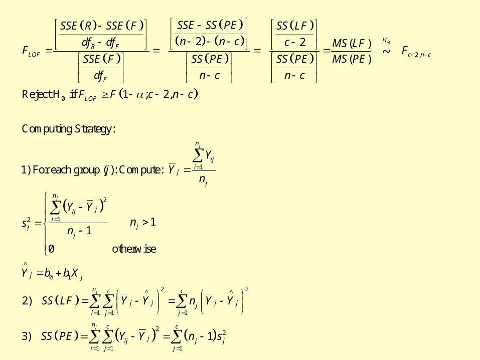
Computing Strategy:

1) For each group ( ): Co

~H

R FLOF c n c

F

LOF

SSE SS PESSE R SSE F SS LF

n n cdf df c MS LFF F

MS PESSE F SS PE SS PE

df n c n c

F F c n c

j

1

2

12

^

0 1

2 2^ ^

1 1 1

22

1 1 1

mpute:

11

0 otherwise

2)

3) 1

j

j

j

j

n

iji

j

j

n

jiji

jjj

j j

n c c

j j j jji j j

n c c

jij j ji j j

YY

n

Y Yns

n

Y b b X

SS LF Y Y n Y Y

SS PE Y Y n s

Height and Weight Data – n=505, c=18 GroupsHeight n Mean SD Y-hat SSLF SSPE SSE

69 2 182.50 3.54 156.95 1305.39 12.50 1317.8971 4 175.75 15.52 169.61 150.62 722.75 873.3772 13 181.00 13.00 175.94 332.27 2028.00 2360.2773 16 186.13 12.09 182.28 237.15 2191.75 2428.9074 21 183.33 9.26 188.61 583.79 1716.67 2300.4575 41 193.71 11.58 194.94 61.96 5360.49 5422.4476 32 200.84 11.96 201.27 5.74 4434.22 4439.9677 31 204.13 10.70 207.60 373.06 3433.48 3806.5578 43 211.00 12.83 213.93 368.86 6912.00 7280.8679 49 221.35 18.70 220.26 57.94 16781.10 16839.0480 46 227.33 15.13 226.59 24.90 10300.11 10325.0181 67 232.49 19.63 232.92 12.30 25430.75 25443.0582 53 241.49 14.79 239.25 265.64 11369.25 11634.8883 44 245.66 17.55 245.58 0.26 13241.89 13242.1484 34 254.62 14.70 251.91 248.66 7128.03 7376.6985 7 247.86 10.75 258.24 755.21 692.86 1448.0786 1 278.00 0.00 264.57 180.24 0.00 180.2487 1 263.00 0.00 270.91 62.50 0.00 62.50

Sum 505 #N/A #N/A #N/A 5026.479 111755.8 116782.3

Source df SS MS F(LOF) F(.95) P-valueLackFit 16 5026.5 314.2 1.369 1.664 0.1521PureError 487 111755.8 229.5

Do not rejectH0: mj = b0 + b1Xj

Box-Cox Transformations

• Automatically selects a transformation from power family with goal of obtaining: normality, linearity, and constant variance (not always successful, but widely used)

• Goal: Fit model: Y’ = b0 + b1X + e for various power transformations on Y, and selecting transformation producing minimum SSE (maximum likelihood)

• Procedure: over a range of l from, say -2 to +2, obtain Wi and regress Wi on X (assuming all Yi > 0, although adding constant won’t affect shape or spread of Y distribution)

11

2 1 11 22

1 0 1

ln 0

nni

i iii

K YW K Y K

KK Y

Box-Cox Transformation – Obtained in R

Maximum occurs near l = 0 (Interval Contains 0) – Try taking logs of Weight

Results of Tests (Using R Functions) on ln(WT)Normality of Errors (Shapiro-Wilk Test)

> shapiro.test(e2) Shapiro-Wilk normality testdata: e2W = 0.9976, p-value = 0.679

> nba.mod2 <- lm(log(Weight) ~ Height)> summary(nba.mod2)

Call:lm(formula = log(Weight) ~ Height)

Coefficients: Est Std. Error t value Pr(>|t|) (Intercept) 3.0781 0.0696 44.20 <2e-16 Height 0.0292 0.0009 33.22 <2e-16

Residual standard error: 0.06823 on 503 degrees of freedomMultiple R-squared: 0.6869, Adjusted R-squared: 0.6863 F-statistic: 1104 on 1 and 503 DF, p-value: < 2.2e-16

Constant Error Variance (Breusch-Pagan Test)> bptest(log(Weight) ~ Height,studentize=FALSE) Breusch-Pagan test

data: log(Weight) ~ HeightBP = 0.4711, df = 1, p-value = 0.4925

Linearity of Regression (Lack of Fit Test) nba.mod3 <- lm(log(Weight) ~ factor(Height))> anova(nba.mod2,nba.mod3)Analysis of Variance Table

Model 1: log(Weight) ~ HeightModel 2: log(Weight) ~ factor(Height) Res.Df RSS Df Sum of Sq F Pr(>F)1 503 2.3414 2 487 2.2478 16 0.093642 1.268 0.2131

Model fits well on all assumptions