Embed Size (px)
Citation preview
Checking Robustness of
Longitudinal Results Across
Two Types of Gain Scores
Robert E. Larzelere, Mwarumba Mwavita, Taren M. Swindle, Ronald B.
Cox, Jr., & Isaac J. Washburn
Oklahoma State Univ. & Univ. of Arkansas for Medical Sciences
2015 Modern Modeling Methods Conference
Overview
Six (or seven) reasons to check whether
longitudinal results replicate for two types
of gain scores
Simple gain scores
Residualized gain scores (e.g,. ANCOVA)
Estimating results for one gain score in
studies that report analyze only one type
Residualized v. simple gain
scores useful because . . . Robustness-checking needed
Biased in opposite directions
r (Y2 ,X1 |Y1 ) biased against corrective actions
r ((Y2 - Y1 ), X1) biased for corrective actions
Results agree if causal estimate unbiased
Tiny b: residual confound or true effect?
Do conclusions depend on residual bias?
Check other causal-inference methods

1. Improving Causal Evidence
with Robustness Checking Source: Duncan et al. (2014)
Show robustness across 2+ analyses
66% -- Applied economics journals
5% -- Developmental psych. journals
Example: Magnuson et al. (2007)
Regression with many covariates
Propensity score matching
Instrumental variable methods
Robust Checks Require Better
Methods or Contrasting Biases Better causality methods: Magnuson e.g.
Robustness w similar biases not helpful
Campbell & Boruch (’75) re Head Start
• 6 methods, all biased against corrective actions
Exact replications worthless if they replicate a
systematic bias (Larzelere et al., 2015, PPS)
2 types of gain scores
Contrasting biases
• for & against corrective actions (define)
2. Two Gain Scores:
Contrasting Bias Residualized gain: r (Y2 ,X1 |Y1 )
PredictingY2 from X1 controlling for Y1
Biased in direction of Y1 differences
Simple gain: r ((Y2 - Y1 ), X1)
Predicting Y2 – Y1 from X1
Biased in opposite direction of Y1
• Due to regression toward the mean
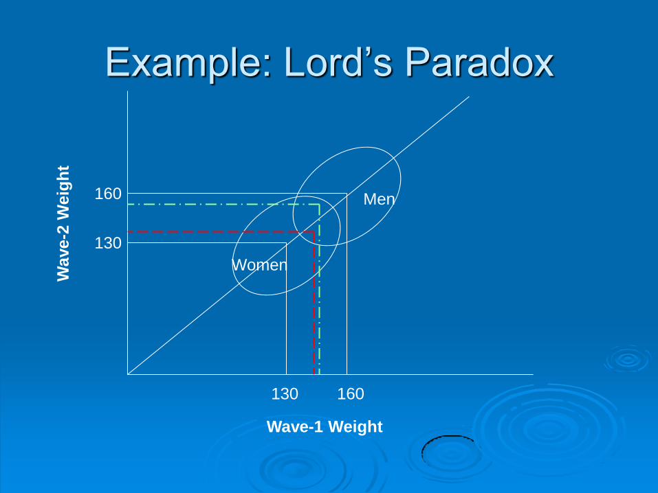
Example: Lord’s Paradox
Wave-1 Weight
Men
Women
130 160
160
130
Wa
ve-2
Weig
ht
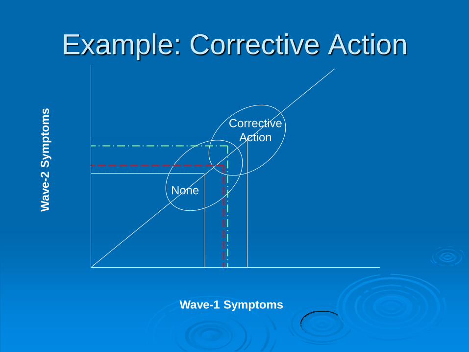
Example: Corrective Action
Wave-1 Symptoms
Corrective
Action
None
Wave-2
Sym
pto
ms
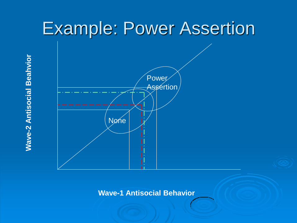
Example: Power Assertion
Wave-1 Antisocial Behavior
Power
Assertion
None
Wave-2
An
tiso
cia
l B
eah
vio
r
Predicting Y2 |Y1 from X1 Biased
Against Corrective Actions BY PARENTS
Physical punishment (Straus et al., 1997;
Ferguson, 2013)
Nonphysical punishments (Larzelere et al.,
2010a, 2010b)
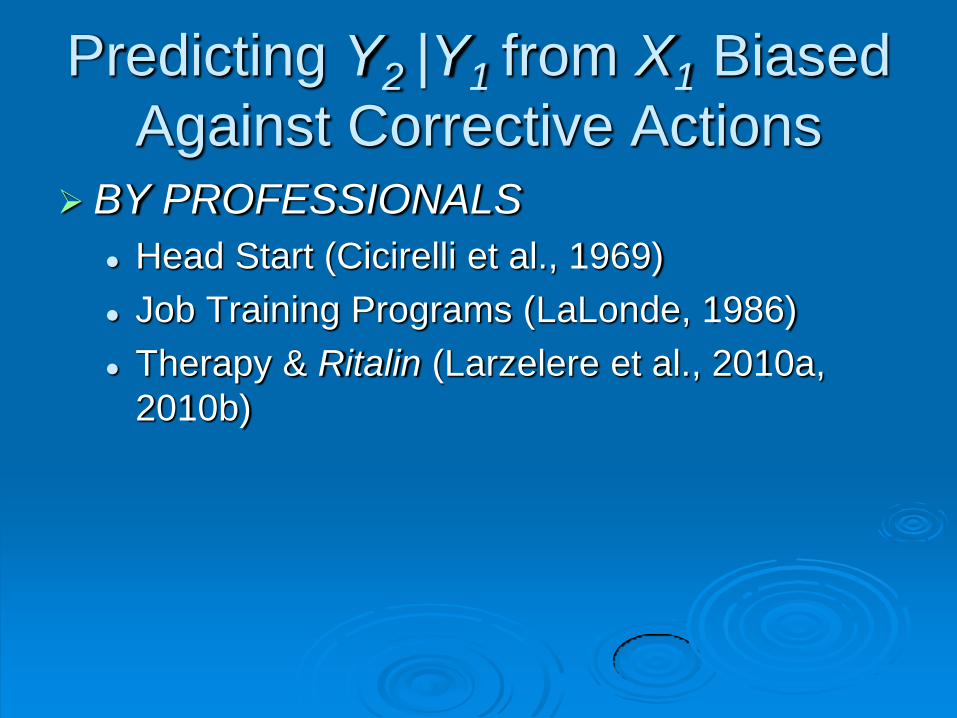
Predicting Y2 |Y1 from X1 Biased
Against Corrective Actions BY PROFESSIONALS
Head Start (Cicirelli et al., 1969)
Job Training Programs (LaLonde, 1986)
Therapy & Ritalin (Larzelere et al., 2010a,
2010b)
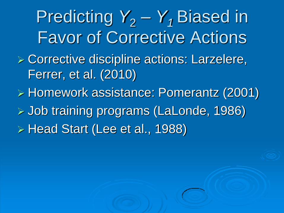
Predicting Y2 – Y1 Biased in
Favor of Corrective Actions Corrective discipline actions: Larzelere,
Ferrer, et al. (2010)
Homework assistance: Pomerantz (2001)
Job training programs (LaLonde, 1986)
Head Start (Lee et al., 1988)
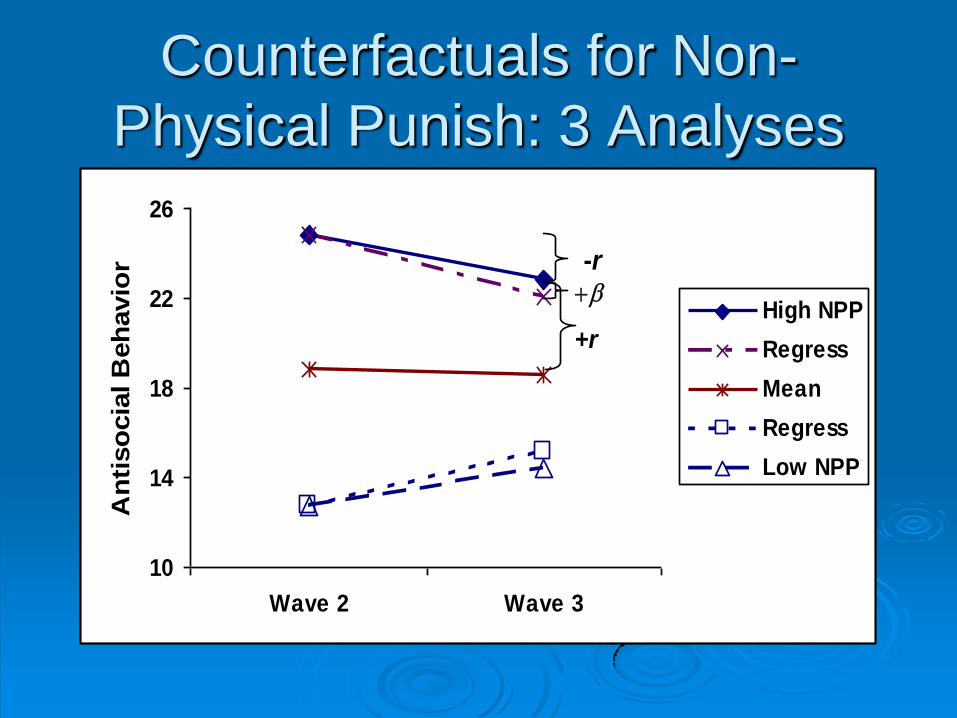
10
14
18
22
26
Wave 2 Wave 3
An
tiso
cia
l B
eh
avio
r
High NPP
Regress
Mean
Regress
Low NPP
b
+r
-r
Counterfactuals for Non-
Physical Punish: 3 Analyses
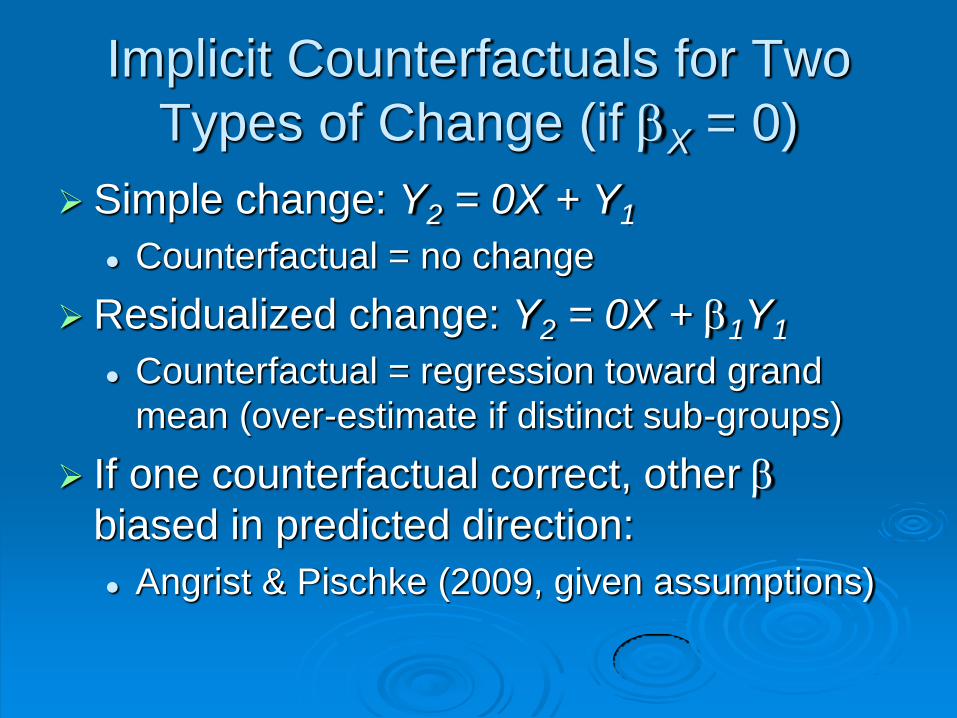
Implicit Counterfactuals for Two
Types of Change (if bX = 0)
Simple change: Y2 = 0X + Y1
Counterfactual = no change
Residualized change: Y2 = 0X + b1Y1
Counterfactual = regression toward grand
mean (over-estimate if distinct sub-groups)
If one counterfactual correct, other b
biased in predicted direction:
Angrist & Pischke (2009, given assumptions)
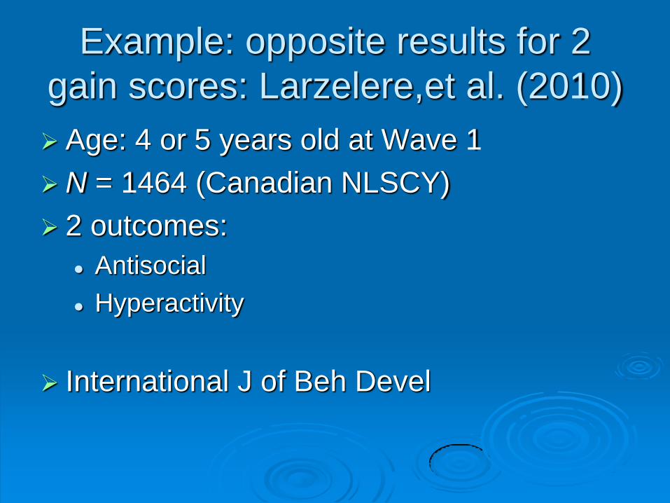
Example: opposite results for 2
gain scores: Larzelere,et al. (2010)
Age: 4 or 5 years old at Wave 1
N = 1464 (Canadian NLSCY)
2 outcomes:
Antisocial
Hyperactivity
International J of Beh Devel
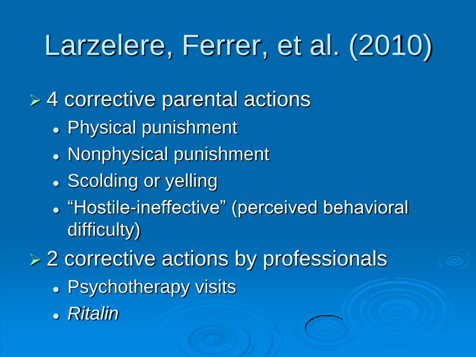
Larzelere, Ferrer, et al. (2010)
4 corrective parental actions
Physical punishment
Nonphysical punishment
Scolding or yelling
“Hostile-ineffective” (perceived behavioral
difficulty)
2 corrective actions by professionals
Psychotherapy visits
Ritalin

Results for Corrective Actions
Correlations (X2, Y3) Unanimously detrimental
Residualized change – all “effects” detrimental
Longitudinal net-effects – 9 of 12 significant, p < .05
Cross-lagged latent analysis – 3 of 12
Simple gains – all “effects” beneficial
r with subsequent gain – 4 of 12
Growth curve – 5 of 12
After reversing waves, same pattern
Evidence of artifact (Galton, 1886; Campbell
& Kenny, 1999)
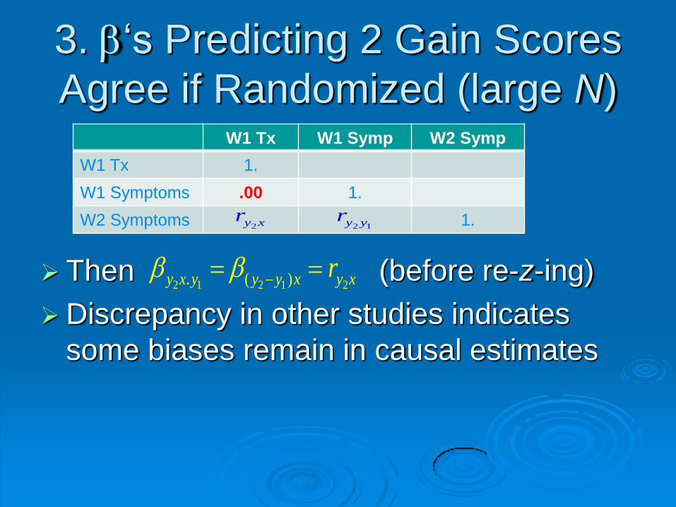
3. b‘s Predicting 2 Gain Scores
Agree if Randomized (large N)
Then (before re-z-ing)
Discrepancy in other studies indicates
some biases remain in causal estimates
W1 Tx W1 Symp W2 Symp
W1 Tx 1.
W1 Symptoms .00 1.
W2 Symptoms 1. 2y xr2 1y yr
2 1 2 1 2. ( )y x y y y x y xrb b
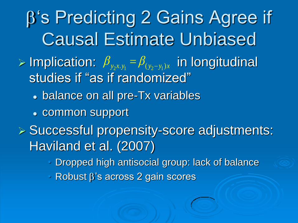
b‘s Predicting 2 Gains Agree if
Causal Estimate Unbiased
Implication: in longitudinal
studies if “as if randomized”
balance on all pre-Tx variables
common support
Successful propensity-score adjustments:
Haviland et al. (2007) • Dropped high antisocial group: lack of balance
• Robust b’s across 2 gain scores
2 1 2 1. ( )y x y y y xb b
4. Small b’s: residual bias or
true causal effect? Large effects more likely to replicate for
both gain scores
Small effects more likely to become n.s. or
change sign for other gain score
Using aspirin to reduce heart attacks: tiny
effect
Are tiny effects from longitudinal data as
compelling?
5. Helps evaluate residual bias
due to untested assumptions Assumptions for unbiased causal
estimates often untestable or untested
Checking robustness across both gain
scores can be an indicator of residual bias
6. Assessing other methods to
improve causal estimates Shows bias reduction from other methods
Propensity score method: Haviland et al. (’07)
Minimizing measurement error
• Showed that measurement error in Y1 biases both
gain scores against corrective actions (Larzelere et
al., submitted)
7. Comparing 2 gain scores
easy to do Easily & widely applicable
Reviewing manuscripts
Post-publication critique
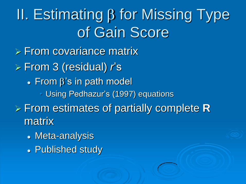
II. Estimating b for Missing Type
of Gain Score From covariance matrix
From 3 (residual) r’s
From b’s in path model
• Using Pedhazur’s (1997) equations
From estimates of partially complete R
matrix
Meta-analysis
Published study
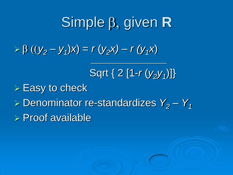
Simple b, given R
b ((y2 – y1)x) = r (y2x) – r (y1x) _____________________
Sqrt { 2 [1-r (y2y1)]}
Easy to check
Denominator re-standardizes Y2 – Y1
Proof available
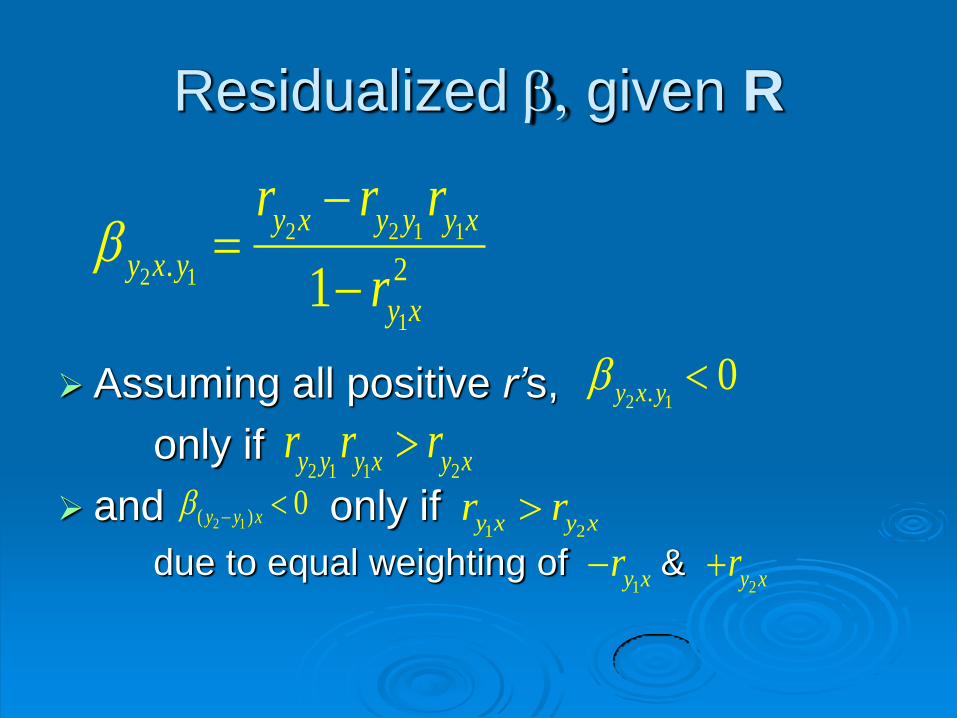
Residualized b, given R
Assuming all positive r’s,
only if
and only if
due to equal weighting of &
2 2 1 1
2 1
1
. 21
y x y y y x
y x y
y x
r r r
rb
2 1. 0y x yb
2 1 1 2y y y x y xr r r
2 1( ) 0y y xb 1 2y x y xr r
1y xr2y xr
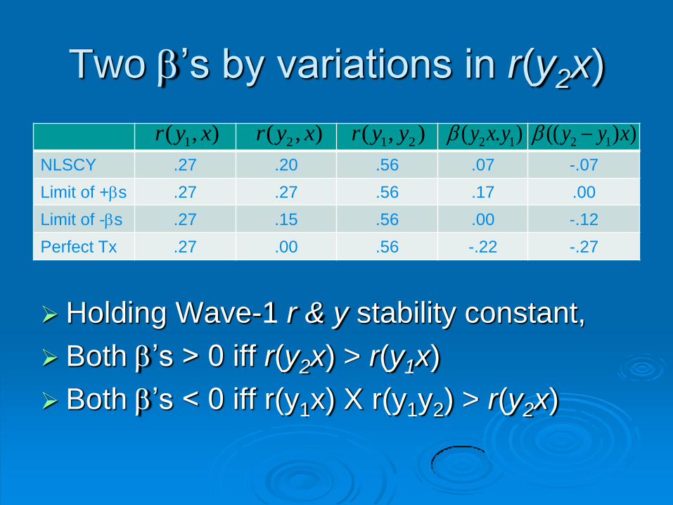
Two b’s by variations in r(y2x)
Holding Wave-1 r & y stability constant,
Both b’s > 0 iff r(y2x) > r(y1x)
Both b’s < 0 iff r(y1x) X r(y1y2) > r(y2x)
NLSCY .27 .20 .56 .07 -.07
Limit of +bs .27 .27 .56 .17 .00
Limit of -bs .27 .15 .56 .00 -.12
Perfect Tx .27 .00 .56 -.22 -.27
1( , )r y x 2( , )r y x 1 2( , )r y y 2 1( . )y x yb 2 1(( ) )y y xb
Checking from R or S matrix
Use latent growth model to test effect of X
on simple gain scores (slope)
Mplus code for 2-wave example in handout
Estimating R to analyze other
gain score Meta-analysis
• Gershoff (2002)
• If meta-analyses estimate all 3 r’s, they could yield
causally relevant estimates from correlational
studies
Individual study examples
• Straus et al. (1997)
• Berlin et al. (2009)
• Levin et al. (1997) on helping with homework
Implications
ANCOVA more biased against corrective
actions than simple gain score analysis
Under what conditions do b’s . . .
agree?
• If balanced, e.g., by propensity-score methods
bracket unbiased causal effect?
• If strongly ignorable given model
• Sometimes unbiased effect is outside both b’s
b’s discrepancy suggests caution, humility
Evidence that 2 b’s may not bracket true b
LaLonde (1986)
• True b outside range of 2 b’s
• Biased in one direction for men, other for women
Need more clarifying research on this,
since predicting change is fundamental to
many areas of research
Implications (cont’d)
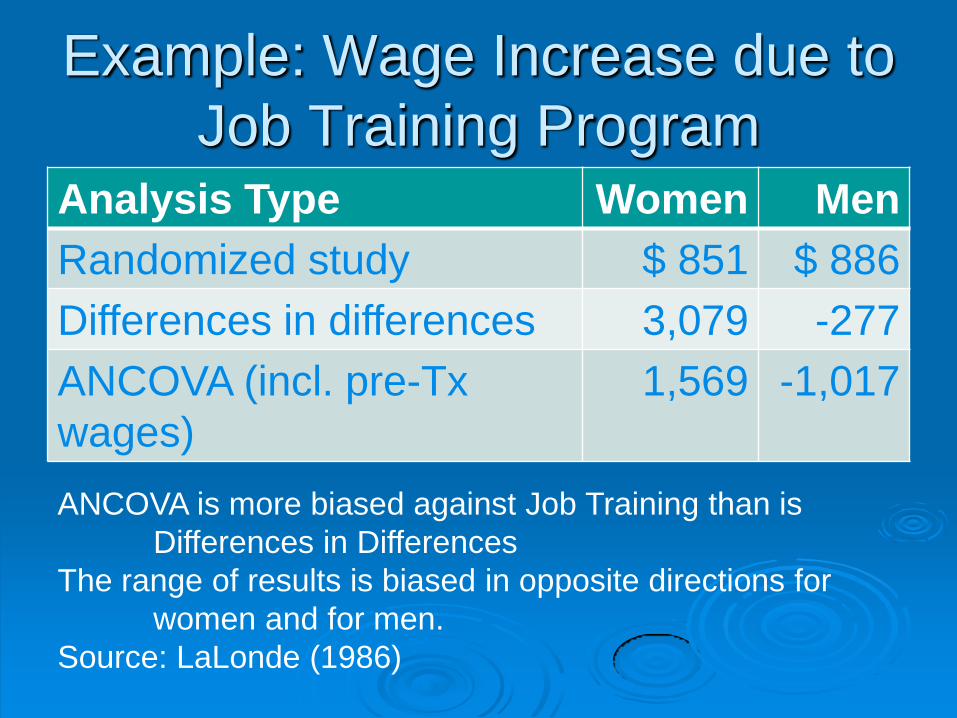
Example: Wage Increase due to
Job Training Program Analysis Type Women Men
Randomized study $ 851 $ 886
Differences in differences 3,079 -277
ANCOVA (incl. pre-Tx
wages)
1,569 -1,017
ANCOVA is more biased against Job Training than is
Differences in Differences
The range of results is biased in opposite directions for
women and for men.
Source: LaLonde (1986)

Thank you!
Co-authors
NIMH funding: R03 HD044679
Support from Oklahoma State University
[email protected] for more
information