Embed Size (px)
Citation preview
Chemical and Biological Oxidation of Naphthenic Acids - where Stoichiometry, Kinetics
and Thermodynamics Meet
by
Reza Mahour
A thesis submitted in partial fulfillment of the requirements for the degree of
Master of Science
in
Environmental Engineering
Department of Civil and Environmental Engineering
University of Alberta
© Reza Mahour, 2016
ii
ABSTRACT
Open-pit mining of Alberta’s oil sands deposits heavily depend on freshwater for the extraction
of bitumen. It leaves 1.25 m3 oil sands process affected water (OSPW) per barrel of produced oil.
In spite of years of research on treatment of OSPW, currently, there are no approved economic
and environmental friendly strategies for management of OSPW. Based on Alberta’s zero
discharge policy, OSPW must be kept on site in custom made tailings ponds that cover
approximately 185 km2 of area. Research results in various fields indicate that naphthenic acids
(NAs) are the main group of complex organics in OSPW that require remediation. NAs have
been shown to be the main contributor to toxicity in OSPW, as well NAs corrode the process
infrastructure. Investigations on the role of indigenous microorganisms in tailings ponds address
their positive effect in removal of NAs. However, a consistent concentration of NAs in aged oil
sands tailings ponds indicates that NAs are not completely biodegradable. Generally, dealing
with recalcitrant compounds, coupling of chemical and biological oxidation is a method of
interest.
Sodium persulfate is an emerging oxidant used in OSPW treatment. Due to the challenging
process of determining chemical composition, and measuring the exact concentration of NAs
mixture in raw samples, for the first time in the field of NAs removal the concept of degree of
reduction has been used for determining the stoichiometric amount of persulfate required for
oxidation of NAs mixture. Estimated required concentrations based on proposed model show
effective outcomes throughout the experiment. It also improved in optimization of the oxidation
process by consuming approximately 5 times less oxidant reported in literature.
iii
To reach the application of combining chemical oxidation by sodium persulfate and
biodegradation, effect of stress of sodium persulfate on Pseudomonas sp. was studied.
Quantitative physiology parameters determined for the bacteria to elucidate the effect of
oxidative stress on their ability to consume NAs. Growth of the bacteria in the presence of
sodium persulfate significantly is affected, which is illustrated by the maximum concentration of
biomass. At 1000 mg/L of sodium persulfate, the maximum concentration of biomass decreased
by ~25 % respect to non-stressed controls. At the dosage of 2000 mg/L, no growth was observed.
However, quantitative physiological analyses showed no significant change in ability of
Pseudomonas sp. for consumption of Merichem NAs (based on DOC). The biomass specific
growth rate (0.1 h-1), biomass specific substrate consumption rate (0.2 mgDOC/mgDCW/h) and
yield of substrate to biomass (0.6 mgDCW/mgDOC) for each persulfate concentration series
were not significantly different.
Thermodynamics is a very powerful tool in understanding the limits of a system and prediction
of possibilities. Some model NAs within literature have indicated to be non-biodegradable, for
example dicyclohexyl acetic acid. To answer the question why dicyclohexyl acetic acid is not
biodegradable, thermodynamics study applied to understand the limits and predict the
possibilities for biodegradation. The University of Minnesota Biocatalysis/Biodegradation
database was used for prediction of possible catabolic pathways for biodegradation of
dicyclohexyl acetic acid. Interestingly, thermodynamics suggest the possibility of biodegradation
under aerobic conditions. Results from bio-thermodynamics analyses predict that dicyclohexyl
acetic acid can be consumed by bacteria with the maximum yield of 0.6 g organic dry weight per
g of dicyclohexyl acetic acid. A 13% relative error has previously been shown with the approach
used in bio-thermodynamics studies. Therefore, thermodynamics can provide a foundation for

iv
future for metabolic and genetic engineers to engineer microorganisms or microbial cultures with
the objective of NAs biodegradation.
v
PREFACE
This thesis is an original work by Reza Mahour under supervision of Dr. Ania Ulrich.
The research completed in chapter 3 was planned, designed, conducted, analyzed, and compiled
by myself. Chapter 4 of this work was planned and designed by Dr. Ania Ulrich and conducted,
analyzed, and compiled by myself.
Chapter 5 of this thesis planned and designed by myself with collaboration of Prof. Sef Heijnen
at Delft University of Technology and Prof. Urs von Stockar at École Polytechnique Fédérale de
Lausanne.

vi
To my mom’s anxieties
To my dad’s hands
To my sister’s kindness
To my brother’s jokes...
vii
ACKNOWLEDGEMENTS
I always liked non-equilibrium thermodynamics since it tells you what is going on in the
dynamic process! Because it gives you the idea of how to appreciate life! I mean it
mathematically proves that you should enjoy the road not just by destination...sometimes a view
on your road it is not as much as beautiful as you supposed it would be, but travel mates can turn
the undesirable view into desirable ones. Dr. Ulrich, you were not only my supervisor but also
you have been a great friend. You taught me that to be an active listener and you didn’t just tell
me that, you showed me by listening to me. You cared about my strengths and weaknesses, so
now I understand what they are, and most of all you trusted me. Thank you Dr. Ulrich, great
thanks!
The thermodynamics section of this thesis would have not been possible without invaluable
comments of Prof. Dr. ir. Sef Heijnen (TU Delft, NL) and Prof. Urs von Stockar (EPFL, CH), I
greatly appreciate your time and help for answering my countless questions. Dr. Vinay Prasad’s
comments about statistical analysis of experimental data is acknowledged.
I would like to acknowledge my supervisor Dr. Thomas Rexer at my research stay at Max Planck
Institute of Dynamics of Complex Technical Systems. Thomas, thank you for all you have done
for me during my stay in Germany. I will never forget your help and memories that we had in
Magdeburg.
I also like to say thanks to my lab mates in Bioremediation Engineering group. Specifically, Dr.
Dena Cologgi, Dr. Hamed Mahdavi and Sarah Miles. Thanks Dena for helping me to set-up my
experiments. Thank you Hamed for your comments on working with naphthenic acids and
teaching me statistical analysis. Hamed, you really are a great friend. Sarah, thank you for being
a very good friend of mine. I will never forget your help to me for integrating into Canadian
culture. And also thanks for your help in editing my thesis.
I am grateful to my funders, NSERC of Canada, Graduate Student Travel Award the Faculty of
Graduate Studies and Research and Graduate Student Association at the University of Alberta.

viii
I also like to say my thanks to my sister Nasim for being a great support. Khahari, you know that
you are a huge part of my life, I always have and will be proud of having a sister and friend like
you.
I’m also thankful to my friends in Edmonton who helped me in various aspects of life. My first
friend in Canada, Vahid who always motivates me to follow my ideas. Thank you Ahura for
being my Dai Asdola, you have always been like my elder brother! My awesome roommates
Firouz and Ramin (I will never ever forget that how many times you guys asked me to make sure
that I have enough funding for my trip to Germany). Thank you Parinaz for being my best friend
and dance partner! I also thank to my friend Ehsan for the great time we had playing foosball and
billiard. Thanks Behnam for our fruitful discussions in Tim Hortons in ETLC! Shiva, thanks for
your help in editing. Thanks to Amir and Amirhossein for the good times we had. Special thanks
to Masoud, Mohammadreza and Farzin (and Naser) for their beautiful minds and their nice
comments about life! Masoud, you have been more than a friend to me. And great thanks to my
very good friends for being good friends.
At the end, I want to hug my mom and dad to say I love you. One of the very best moments of
life is when you realize that your parents are actually your best friends and I feel so blessed that I
experienced this feeling so many times. Thank you for being my parent and my closest friends.
Oh you read the whole acknowledgment! Thank you to you too!
April, 2016
Edmonton, Canada
ix
TABLE OF CONTENTS
1. CHAPTER 1. INTRODUCTION AND RESEARCH OBJECTIVES ............................................... 1
1.1 General Introduction ................................................................................................................ 1
1.2 Purpose of Study ...................................................................................................................... 7
1.3 Organization of Thesis ............................................................................................................. 8
1.4 References ............................................................................................................................... 9
2 CHAPTER 2. LITERATURE REVIEW ........................................................................................ 13
2.1 Introduction ........................................................................................................................... 13
2.2 Naphthenic Acids ................................................................................................................... 14
2.2.1 Properties of Naphthenic Acids ....................................................................................... 15
2.2.2 Application of Napphthenic Acids .................................................................................. 16
2.2.3 Disadvantages of Naphthenic Acids ................................................................................ 17
2.2.3.1 Corrosive to process infrastructures ............................................................................ 17
2.2.3.2 AEOs Toxicity............................................................................................................ 18
2.2.4 Quantification of Naphthenic Acids ................................................................................ 19
2.2.5 Treatment of OSPW and NAs contaminated wastewater ................................................. 20
2.2.5.1 Chemical Treatment.................................................................................................... 20
2.2.5.2 Biological Treatment .................................................................................................. 24
2.2.5.3 Coupling of Chemical and Biological Remediation ..................................................... 27
2.3 Oxidative Stress ..................................................................................................................... 28
2.4 Bioremediation Kinetics and Stoichiometry ............................................................................ 30
2.4.1 Kinetic and Stoichiometric Analysis of bioremediation: Quantitative Physiology ............ 31
2.4.2 Biomass Specific Rate: q-rate ......................................................................................... 33
2.4.3 Biodegradation Thermodynamics ................................................................................... 34
2.4.3.1 Importance of Thermodynamics Analysis ................................................................. 35
2.4.3.2 Thermodynamics of Naphthenic Acids biodegradation .............................................. 35
2.5 References ............................................................................................................................. 37
CHAPTER 3. STOICHIOMETRIC DETERMINATION OF PERSULFATE DOSES FOR OXIDATION
OF ACID EXTRACTABLE ORGANICS ............................................................................................. 45
3.1 Introduction ........................................................................................................................... 45
3.2 Materials and Methods ........................................................................................................... 48
3.2.1 Chemicals and Material Preparation ................................................................................ 48
x
3.2.2 Kinetic Experiments ....................................................................................................... 49
3.2.3 Analytical Methods ........................................................................................................ 49
3.3 Results and Discussion ........................................................................................................... 50
3.3.1 Fundamentals of Proposed Model ................................................................................... 50
3.3.2 Determination of Required Dosage of Oxidant ................................................................ 52
3.3.3 Application of Proposed Model to other Oxidants ........................................................... 56
3.4 References ............................................................................................................................. 60
CHAPTER 4. OXIDATIVE STRESS INFLUENCE ON BIODEGRADATION: QUANTITATIVE
PHYSIOLOGICAL STUDY ................................................................................................................. 64
4.1 Introduction ................................................................................................................................. 64
4.2 Materials and Methods ........................................................................................................... 69
4.2.1 Substrate, Oxidant and Microorganism Used in Experimental Set-up .............................. 69
4.2.2 Measurement of Cell Growth and DOC .......................................................................... 70
4.2.3 Oxidative Stress Test ...................................................................................................... 70
4.2.4 Biodegradation Experiment ............................................................................................ 71
4.3 Results and Discussion ........................................................................................................... 72
4.3.1 Biodegradative Capacity of Pseudomonas sp. ................................................................. 72
4.3.2 Impact of Persulfate Oxidative Stress on Pseudomonas sp .............................................. 72
4.3.3 Mass Transfer Analysis .................................................................................................. 75
4.3.3.1 Oxygen Mass Transfer Coefficient in Gas Phase ........................................................ 75
4.3.3.2 Oxygen Mass Trasnfer Coefficient in Liquid Phase .................................................... 76
4.3.4 Biodegradation of Merichem Naphthenic Acids Post Oxidative Stress ............................ 77
4.3.5 Mathematical Modelling Based on Mass Balance ........................................................... 79
4.3.5.1 Biomass specific growth rate ...................................................................................... 87
4.3.5.2 Yield of Substrate to Biomass (Ysx)............................................................................. 88
4.3.5.3 Biomass Specific Substare Consumption Rate (qs) ...................................................... 89
4.3.6 Lag Time of Biodegradation ............................................................................................ 90
4.4 Conclusions ........................................................................................................................... 90
4.5 References ............................................................................................................................. 92
CHAPTER 5. THERMODYNAMICS OF NAPHTHENIC ACIDS BIODEGRADATION UNDER
AEROBIC CONDITION ..................................................................................................................... 101
5.1 Introduction ......................................................................................................................... 101
5.2 Cellular Growth Concepts .................................................................................................... 103
xi
5.2.1 Cellular Metabolism ..................................................................................................... 103
5.2.1.1 Catabolism .............................................................................................................. 103
5.2.1.2 Anabolism ................................................................................................................ 106
5.2.1.3 Maintenance ............................................................................................................. 107
5.3 Thermodynamics Background .............................................................................................. 108
5.3.1 Equilibrium Thermodynamics....................................................................................... 108
5.3.2 Non-Equilibrium Thermodynamics ............................................................................... 109
5.3.3 Free Energy Dissipation in Spontaneous Process........................................................... 113
5.3.4 Entropy Production in a Continuous System ................................................................. 116
5.3.5 Thermodynamic Coupling ............................................................................................. 118
5.3.6 Chemical Reatcion as One of the Examples of Force-Flow Relation and Reciprocal
Relation ....................................................................................................................................... 121
5.3.7 Phenomenological non-Equilibrium Thermodynamics and Microbial Growth ................ 124
5.4 Thermodynamics of Microbial Growth ................................................................................. 126
5.4.1.1 Prediction of Substrate Needed for Maintenance ..................................................... 127
5.4.1.1.1 Required Substrate for Maintenance .................................................................. 127
5.4.1.1.2 Required Energy for Maintenance ..................................................................... 128
5.4.1.2 Prediction of Gibbs Energy Needed for Growth ....................................................... 129
5.4.1.3 Prediction of Biomass Maximum Specific Growth Rate (µmax) ................................. 132
5.5 Case Study: Biodegradation of Model Naphthenic Acids ........................................................ 133
5.5.1 Catabolic Pathways ......................................................................................................... 134
5.5.2 in silico Biodegradation of Dicyclohexyl acetic acid ........................................................ 136
5.5.2.1 Catabolism of Dicyclyhexyl acetic acid..................................................................... 136
5.5.2.2 Anabolism ................................................................................................................ 141
5.5.2.1.1 Calculation of µmax ............................................................................................ 145
5.5.2.3 Needed Substrate for Maintenance ............................................................................. 145
5.5.3 Simulation of the stoichiometric and kinetics parameters .................................................. 147
5.5.3.1 Estimation of Substrate Affinity ................................................................................. 149
5.6 Conclusion ........................................................................................................................... 151
5.7 References ........................................................................................................................... 153
CHAPTER 6. CONCLUSIONS AND RECOMMENDATIONS .......................................................... 160
6.1 Thesis Overview .................................................................................................................. 160
6.2 Summary of Findings ........................................................................................................... 160
xii
6.3 Significance of the Research ................................................................................................ 164
6.4 Recommendations for Future Work ...................................................................................... 164
BIBLIOGRAPHY ............................................................................................................................... 169
APPENDIX 1: SUPPLEMENTARY DATA FOR CHAPTER 3 .......................................................... 192
APPENDIX 2: SUPPLEMENTARY DATA FOR CHAPTER 4 .......................................................... 196
APPENDIX 3: SUPPLEMENTARY DATA FOR CHAPTER 5 .......................................................... 208
xiii
LIST OF TABLES
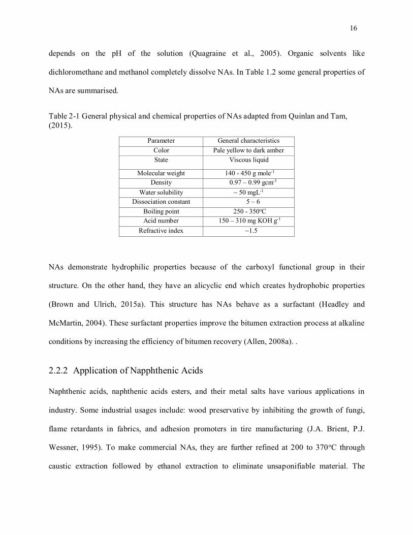
Table 2-1 General physical and chemical properties of NAs adapted from Quinlan and Tam, (2015). ..... 16
Table 2-2 Common oxidants for chemical oxidation treatment goals (Siegrist et al., 2011). .................... 22
Table 3-1. Kinetic constants of first order rate; mean multicomparison statistical analyses conducted to
determine the significany of differences between treatments (See Appendix A.1); statistical analyses
results show that all treatments are significantly different (p < 0.05) except treatments D and 2D
(p=0.359) based on Tukey’s test ............................................................................................................ 55
Table 3-2 Comparisosn of result of this work and relevant literature ...................................................... 55
Table 3-3 Estimation of the cost of treatment process, and comparison of the cost based on different
methods. Total volume of water in MLSB is reported by Syncrude and cost of the sodium persulfate
considered as 2.7 $ per kg (Chen et al., 2015) ........................................................................................ 56
Table 4-1 Treatment conditions to test the biodegradative capacity of oxidatively stressed Pseudomonas
sp. isolates. ............................................................................................................................................ 71
Table 4-2. Maximum biomass concentration (in absorbance unit (AU) @600 nm) under different
persulfate oxidant concentrations. Data are shown ± standard error of triplicate ..................................... 74
Table 4-3. Oxygen mass transfer coefficient in the gas phase is calculated. V shows the volume of the
flask, L represents the liquid volume of the flask; N is the mixing rate; α is constant and TG is turbulence
factor which is calculated based on Eq. 4.27. ......................................................................................... 76
Table 4-4. Calculated related parameters for estimation of oxygen mass transfer coefficient in liquid
phase;1 litre flasks used as a bioreactor with the effective liquid volume of 0.5 L (broth) ....................... 77
Table 4-5. Biomass specific growth rate and doubling time of biomass .................................................. 87
Table 4-6. Yield of substrate to biomass for non-stressed and previously stressed bacteria ..................... 88
Table 4-7. Biomass specific substrate consumption rate for different oxidatively stressed bacteria ......... 89
xiv Table 5-1 Catabolic reactions of some organic compounds under various electron accepting condition;
redox couple of NO3 -1/N2 and CO2 / CH4 are representing denitrification and methanogen condition,
respectively (Smolke, 2009) ................................................................................................................ 105
Table A-1Statistical results of multiple comparison of 0.25, 0.5, 1 and 2 times of D; p-value is shown as
“Sig” ................................................................................................................................................... 193
Table A1-2. Degree of reduction of common elements ......................................................................... 194
Table A2-1. Statistical analysis of maximum concentration of biomass ................................................ 197
Table A2-2. Statistical analysis of maximum concentration of biomass ................................................ 198
Table A2-3. Statistical analysis of yield of substrate to biomass ........................................................... 199
Table A2-4. Statistical analysis of biomass specific substrate consumption rate.................................... 200
Table A3-1. Structural groups used in group contribution method for estimation of Gibbs free energy of
formation............................................................................................................................................. 211
Table A3-2. Participated groups in calculation Gibbs energy of formation of C11 H20 O2 ....................... 212
Table A3-3Two model NAs for determination of thermodynamic favourability of catabolic pathwyas . 213
xv
LIST OF FIGURES
Figure 1-1 Connection of the three fundamental concepts of a reaction .................................................... 5
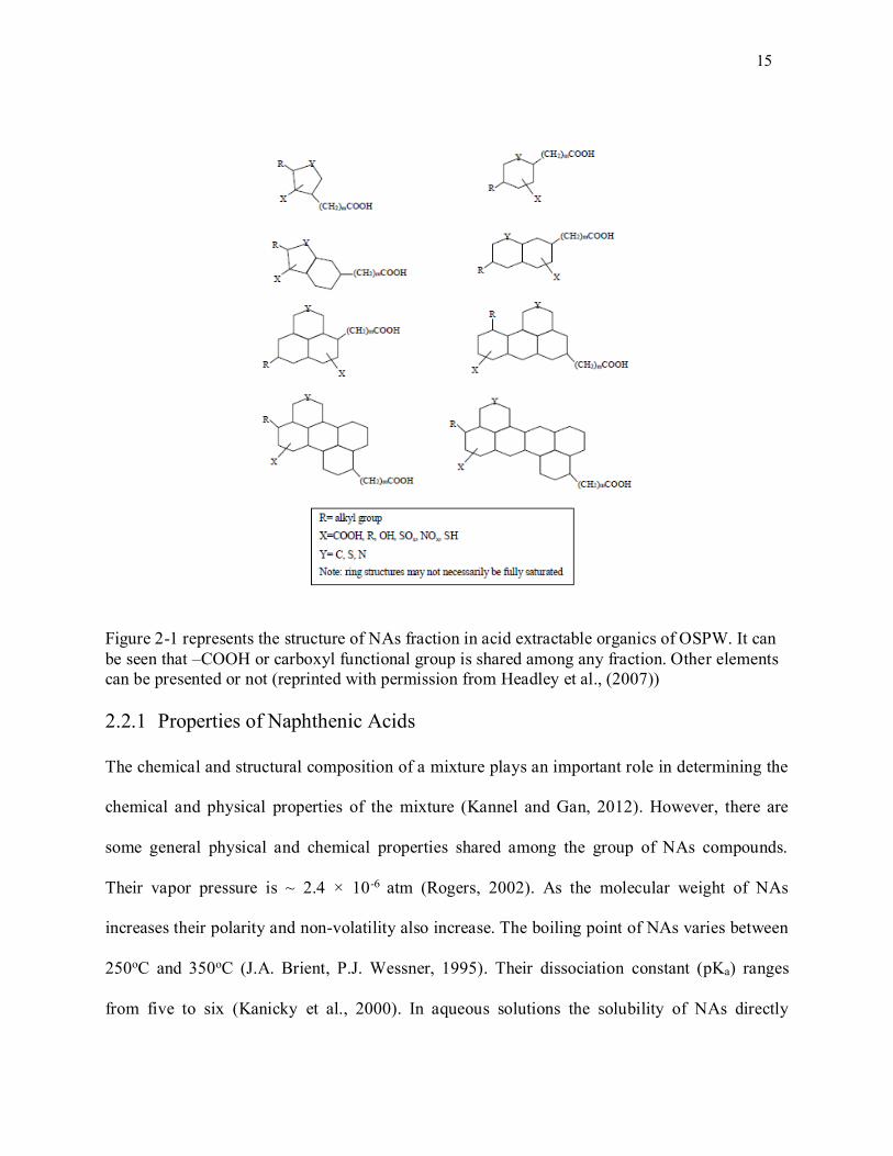
Figure 2-1 represents the structure of NAs fraction in acid extractable organics of OSPW. It can be seen
that –COOH or carboxyl functional group is shared among any fraction. Other elements can be presented
or not (reprinted with permission from Headley et al., (2007))........................................................ 15
Figure 2-2 Proposed corrosion mechanisms by NAs at high temperature (reprinted with permission from
Chakravarti et al., (2013)). ..................................................................................................................... 17
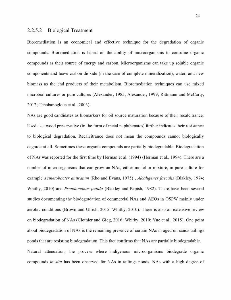
Figure 2-3. Difference between biodegradation of commercial NAs and NAs in AEOs from OSPW. ..... 26
Figure 2-4. Reduction of oxygen to water; the redox potential of O2; O2-; H2O2; HO˖ are presented (in
volt), respectively; potentially all compounds except oxygen are oxidant. (reprinted with permission from
Imlay (2013)); The oxidants in this figure are known as the intracellular oxidants. However,
environmental (extracellular) oxidizing agents can cause injuries to cell. ............................................... 28
Figure 3-1. Degradation of NAs (carboxylic acids) vs. time based on FTIR............................................ 54
Figure 3-2. The linear regression analysis of degradation data to first order rate model; shows the samples
.............................................................................................................................................................. 54
Figure 4-1. Growth of Pseudomonas sp. in LB broth; Graph (I) represents growth under zero stress;
Graph (A) illustrates growth under 250 mg/L of Na2S2O8; Graph (B) illustrates growth under 500 mg/L of
Na2S2O8; Graph (C) illustrates growth under 1000 mg/L of Na2S2O8; Graph (D) illustrates growth under
2000 mg/L of Na2S2O8; Error bars are plus minus of standard error of triplicate ..................................... 73
Figure 4-2. Biodegradation of Merichem NAs under aerobic condition by Pseudomonas sp. isolated from
oil sands tailings pond. Series (I) represents the non-stressed bacteria; (A) shows the bacteria previously
stressed with 250 mg/L sodium persulfate; (B) bacteria stressed with 500 mg/L and (C) with 1000 mg/L
of sodium persulfate. ( ) represents the dry cell weight (DCW) and ( ) illustrates the concentration of
dissolved organic carbon (DOC); error bars are plus minus standard error.............................................. 84
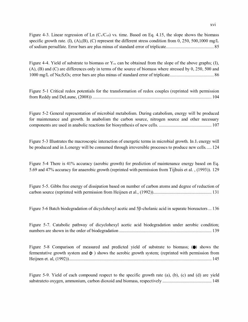
xvi Figure 4-3. Linear regression of Ln (Cx/Cx0) vs. time. Based on Eq. 4.15, the slope shows the biomass
specific growth rate. (I), (A),(B), (C) represent the different stress condition from 0, 250, 500,1000 mg/L
of sodium persulfate. Error bars are plus minus of standard error of triplicate......................................... 85
Figure 4-4. Yield of substrate to biomass or Ysx can be obtained from the slope of the above graphs; (I),
(A), (B) and (C) are differences only in terms of the source of biomass where stressed by 0, 250, 500 and
1000 mg/L of Na2S2O8; error bars are plus minus of standard error of triplicate...................................... 86
Figure 5-1 Critical redox potentials for the transformation of redox couples (reprinted with permission
from Reddy and DeLaune, (2008)) ...................................................................................................... 104
Figure 5-2 General representation of microbial metabolism. During catabolism, energy will be produced
for maintenance and growth. In anabolism the carbon source, nitrogen source and other necessary
components are used in anabolic reactions for biosynthesis of new cells. ............................................. 107
Figure 5-3 Illustrates the macroscopic interaction of energetic terms in microbial growth. In Jc energy will
be produced and in Ja energy will be consumed through irreversible processes to produce new cells. .... 124
Figure 5-4 There is 41% accuracy (aerobic growth) for prediction of maintenance energy based on Eq.
5.69 and 47% accuracy for anaerobic growth (reprinted with permission from Tijhuis et al. , (1993)). 129
Figure 5-5. Gibbs free energy of dissipation based on number of carbon atoms and degree of reduction of
carbon source (reprinted with permission from Heijnen et al., (1992)). ................................................. 131
Figure 5-6 Batch biodegradation of dicyclohexyl acetic and 5β-cholanic acid in separate bioreactors ... 136
Figure 5-7. Catabolic pathway of dicyclohexyl acetic acid biodegradation under aerobic condition;
numbers are shown in the order of biodegradation ............................................................................... 139
Figure 5-8 Comparison of measured and predicted yield of substrate to biomass; ( ) shows the
fermentative growth system and ( ) shows the aerobic growth system; (reprinted with permission from
Heijnen et. al, (1992)) .......................................................................................................................... 145
Figure 5-9. Yield of each compound respect to the specific growth rate (a), (b), (c) and (d) are yield
substrateto oxygen, ammonium, carbon dioxoid and biomass, respectively .......................................... 148
xvii Figure 5-10. Comparison of experimental and in silico biodegradation of dicyclohlohexyl acetic acid with
the same environmental condition (Graph on the right reprinted with permission from Misiti et. al,
(2014)) ................................................................................................................................................ 150
Figure A3-1. Molecular structure of 4-butylcyclohexanecarboxylic acid. ............................................. 212
Figure A3-2. Different catabolic pathways for biodegradation of 4-Butylcyclohexanecarboxylic.......... 214
Figure A3-3. Different catabolic pathways for 4-tert-Butylcyclohexanecarboxylic acid ........................ 214
xviii
LIST OF ACRONYMS
OSPW Oil Sands Process-affected Water
NAs Naphthenic Acids
AEOs Acid Extractable Organics
COD Chemical Oxygen Demand
DOC Dissolved Organic Carbon
OD Optical Density
DCW Dry Cell Weight
DCM Dichloromethane
FTIR Fourier Transform Infrared Spectroscopy
NADH Nicotinamide adenine dinucleotide
ETC Electron Transport Chain
xix
GLOSSARY
𝛾 Degree of reduction
∆𝐺 Gibbs free energy difference across a reaction
𝐾𝑒𝑞 Equilibrium constant
𝑄 Reaction quotient
𝚽 Rate of dissipation of Gibbs free energy, dissipation function
𝜇𝑖 Chemical potential of unexchangeable substance 𝑖
𝜇𝑗 Chemical potential of freely exchangeable substance 𝑗
𝜎𝑠 Entropy production function
ᵭ Small change
ᵭ𝑒 Small change due to exchange with the environment
ᵭ𝑖 Small change due to internal process
ᵭ𝑒𝑄′
Heat exchanged after correction for partial molar enthalpies of
exchanged substabces
ᵭ𝑒𝑄′′
Pure heat exchanged after correction for partial molar enthalpy but
including the entropy of exchanged particles
ᵭ𝑒𝑊 Work
ᵭ𝑒𝑊′ Work including enthalpy import through transport
ᵭ𝑒𝑊′′ Work including transport work
𝑑𝑖𝑣(𝐽𝑥) Divergence of 𝐽𝑥
𝐸 Energy
𝐽𝛼 Flux through branch α
𝐽𝑐ℎ𝑒𝑚 Fluc through chemical reaction
𝐽𝑘 Flux through process k
𝐽𝑞 Heat flow
𝑉 Volume
𝑃 Hydrostatic pressure
𝐹 Elastic
xx
𝑆 Entropy
𝐾𝑠 Substrate affinity
𝑞𝑖 Biomass specific rate of compound 𝑖
𝑌𝑖𝑗 Yield of compound 𝑖 to compound 𝑗
𝜇 Biomass specific growth rate
𝐶1𝐻1.8𝑂0.5𝑁0.2 General formula of biomass
1
1. CHAPTER 1. INTRODUCTION AND RESEARCH
OBJECTIVES
1.1 General Introduction
Oil sands consist of quartz sand grains, covered by a layer of water and clay and then surrounded
by a slick of heavy oil called bitumen (Speight, 2007). Canada’s oil sands deposits are the third
largest oil sands deposits in the world, which contain 1.8 trillion barrels of oil reserves
(Government of Alberta, 2016). 170 billion barrels are located in Alberta with 168 billion barrels
of recoverable bitumen (with today’s technologies). Alberta’s oil sands are found in three
deposits: Athabasca, Cold Lake and Peace River. These three deposits cover an area equal in size
to the province of New Brunswick (Government of Alberta, 2016). One of the most common
methods for oil sands extraction, is hot water extraction which was proposed by Dr. Karl A.
Clark in 1920 (Speight, 2007). This method mixes oil sands with hot water to form a slurry. The
slurry is transported to separation vessels where it is separated into three different layers (from
bottom to top): sand settles to the bottom, middlings which is sand, and clay, water and a layer of
bitumen froth at the top (Government of Alberta, 2016; Speight, 2007). The bitumen froth is
transported to upgrading units for additional processing. The remaining layers of sand, clay and
water from the separation vessel are pumped to large on site custom made tailings ponds for
storage and re-use. Overall, this method produces 1.25 m3 of oil sands process-affected water
(OSPW) for each barrel of oil (Allen, 2008a). Since 1993 any release of these wastewaters into
the environment is prohibited by the Alberta Environmental Protection and Enhancement Act,
Section 23 (1993), commonly referred to as the zero discharge policy (Giesy et al., 2010;
Government of Alberta, 2016). To satisfy the environmental regulations, promote settling of
solids, and mineralization of organics, custom made tailings ponds are constructed on site to
2
collect OSPW (Government of Alberta, 2010). Currently, tailings ponds cover 77 square
kilometers in Alberta (Government of Alberta, 2010). Utilization of OSPW in tailings ponds for
water recycling reduces the dependency to fresh water by 80-85% (Allen, 2008a). However,
recycling OSPW increases concentrations of the minerals, trace metals, residual bitumen, and
organics in OSPW (Allen, 2008a). Therefore, finding an economic, environmentally friendly and
efficient strategy for treatment of OSPW is one of the biggest challenges facing the oil sands
industry (Allen, 2008b).
One consequence of on-site tailings ponds is seepage of OSPW from tailings ponds and their
supporting dykes into the subsurface (Oiffer et al., 2009). There are several studies on the
infiltration of OSPW into the subsurface, groundwater and its subsequent transport to surface
water (Abolfazlzadehdoshanbehbazari et al., 2013; Holden et al., 2011; Holden et al., 2013).
From these studies, the migration of salts, metals and naphthenic acids are a key concern.
Naphthenic Acids (NAs) are natural components of petroleum, which are complex mixtures of
alkyl-substituted acyclic, monocyclic and polycyclic carboxylic acids with the general formula of
CnH2n+zO2 where n represents the number of carbons and z represents the number of rings
(Holowenko, 2002). Concentration of NAs in crude oil varies depending on the source of crude
oil. There are two potential sources that contribute to the presence of NAs in crude oil and oil
sands: biological (diagenesis) and/or geological (catagenesis) (Tissot and Welte, 1978).,
Catagenesis is a physical process that takes place at high temperature (between 50 and 150 0C)
and pressure (Tissot and Welte, 1978). Elimination of carbonyl group (it is also found in NAs) is
occurred at this step. Diagenesis is an anaerobic process where methane and kerogen are
produced by microorganisms (Tissot and Welte, 1978). In general, when petroleum exposed to
non-indigenous bacteria through i.e. earthquake resulted in biodegradation of petroleum (Riva,
3
1983). Carboxylic acids are by-products of biodegradation of crude oil. The presence of
carboxylic acids is found in biodegradable crude oil deposits (Meredith et al., 2000; Nascimento
et al., 1999) and laboratory research on biodegradation of crude oil (Roques et al., 1994; Watson
et al., 2002). NAs in Alberta’s oil sands are mainly by-products of bitumen biodegradation
(Clemente and Fedorak, 2005; Tissot and Welte, 1978). NAs and AEOs need to be extracted
from the aqueous phase to analyse. In literature there are three different type of NAs are
mentioned. First, surrogate NAs which are mainly model NAs with exact molecular formula i.e.
2-Methyl-1-cyclohexanecarboxylic acid (C8H14O2). Second, commercial NAs with suppliers like
Merichem, Kodak which are mainly complex mixture of carboxylic acids. The third one is
known as the OSPW associated NAs. To characterize NAs in OSPW an extraction step with a
proper organic solvent i.e. dichloromethane needs to be conducted at acidic pHs (<2) (Brown and
Ulrich, 2015). Analysis by high resolution analytical instruments show different a composition of
OSPW sourced NAs in comparison of the classical NAs formula CnH2n+zO2. For instance, only
20% of OSPW associated NAs are 2-oxygen NAs (Grewer et al., 2010; Headley and McMartin,
2004). To distinguish between the classic (general formula) and non-classic (OSPW associated)
NAs, the term oil sands tailings water acid-extractable organics (OSTWAEO) or acid extractable
organics (AEOs) should be used. One should realize that NAs are portion of AEOs or in other
words AEOs are some organics plus NAs (Grewer et al., 2010).
NAs (CnH2n+zO2) + Organics = AEOs (1.1)
Understanding which bitumen-derived compounds contribute to the acute toxicity of OSPW is
complex (Klamerth et al., 2015; Morandi et al., 2015). To unravel the toxicity of organics in
OSPW, Morandi et al. (2015) extracted the organics in OSPW at different pHs. Results from this
work have shown that the non-acidic organic portion of OSPW (extracted at pH 11) are less-
4
toxic (Morandi et al., 2015). In contrast, results heavily support that the NAs are the main
compounds that create acute toxicity in OSPW (MacKinnon and Boerger, 1986; Morandi et al.,
2015; Zhang et al., 2011).
After many years of natural attenuation in tailings ponds, the remaining AEOs in aged OSPW are
thought to be resistant to natural attenuation (Allen, 2008b). Application of chemical oxidants
are very common in the treatment of non-biodegradable compounds (Oller et al., 2011).
However, to completely remove the recalcitrant contaminants, utilizing chemical oxidation
strategies is not always applicable due to the resistance of oxidation intermediates to complete
oxidation (Muñoz et al., 2005; Oller et al., 2011). As such more oxidant is added to complete the
oxidation process, which is both costly and time-consuming. One modification to this method is
the use of microorganisms to bioremediate the oxidation intermediates. This process is attractive
because of its low operation costs (Rittmann and McCarty, 2012; Tchobanoglous et al., 2003).
Various studies have shown that chemical oxidation as a pre-treatment step improves the
biodegradability of wastewaters as it converts compounds from recalcitrant to biodegradable
(Brown et al., 2013; Hwang et al., 2013; Martin et al., 2010). Based on this concept, coupling of
chemical and biological oxidation is of interest in treatment of recalcitrant compounds (Oller et
al., 2011). Due to the huge volume of tailings ponds, in situ treatment strategies for treatment of
OSPW are more desirable specifically because of the lower costs. One of the challenges of in
situ coupling of chemical oxidation and biological treatment is vulnerability of micro-organisms
to chemical oxidants. Oxidants (proportional to their dosage and properties) can kill off or
damage the cells because of their high redox potential and high reactivity (Guzel-Seydim et al.,
2004; Veschetti et al., 2003). Many of these oxidants are used as disinfectants i.e. ozone for
drinking water treatment (Camel and Bermond, 1998; Guzel-Seydim et al., 2004). However, our
5
Reaction
lab completed a study demonstrating the survival of indigenous microbes after ozonation with
the purpose of improving biodegradability of aged OSPW (Brown et al., 2013).
A number of issues are associated with working on an OSPW treatment. OSPW is a complex
mixture of organics where the analysis of these organics is a significant challenge (Brown and
Ulrich, 2015). To date, a cost effective and accurate analytical technique for organics whitin
OSPW has not been developed (Brown and Ulrich, 2015). Analytical instruments with different
degrees of accuracy and sensitivity give us different feedback about the real content of organics
either acidic or nonacidic organics (Brown and Ulrich, 2015; Clemente and Fedorak, 2005;
Headley et al., 2013).
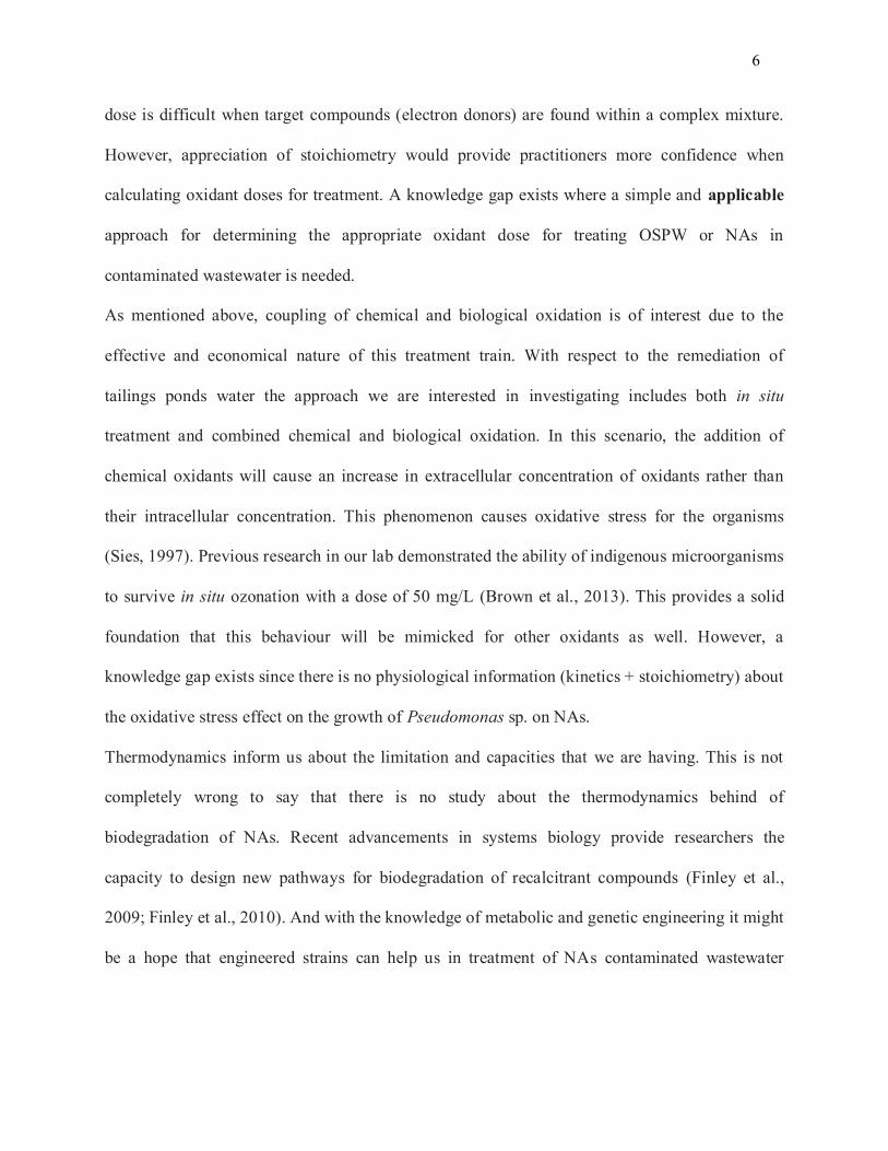
To fully understand any reactions there are three main components to consider: stoichiometry,
kinetics and thermodynamics. Determining these three fundamental components greatly help
environmental engineers in treating wastewaters (as shown in Fig. 1.1).
Figure 1-1 Connection of the three fundamental concepts of a reaction
Without understanding these connections it is difficult to optimize remediation processes. For
instance, persulfate has been shown to be reactive toward NAs (Drzewicz et al., 2012; Sohrabi et
al., 2013). Sohrabi et al. (2013) used 10 g/L of sodium persulfate and 5 g/L of potassium
permanganate (separately) to degrade NAs in OSPW. However, there is no mention in their work
why they chose 10 g/L and 5 g/L oxidant doses. It is understandable that determining oxidant
Stoichiometry
Thermodynamics Kinetics
6
dose is difficult when target compounds (electron donors) are found within a complex mixture.
However, appreciation of stoichiometry would provide practitioners more confidence when
calculating oxidant doses for treatment. A knowledge gap exists where a simple and applicable
approach for determining the appropriate oxidant dose for treating OSPW or NAs in
contaminated wastewater is needed.
As mentioned above, coupling of chemical and biological oxidation is of interest due to the
effective and economical nature of this treatment train. With respect to the remediation of
tailings ponds water the approach we are interested in investigating includes both in situ
treatment and combined chemical and biological oxidation. In this scenario, the addition of
chemical oxidants will cause an increase in extracellular concentration of oxidants rather than
their intracellular concentration. This phenomenon causes oxidative stress for the organisms
(Sies, 1997). Previous research in our lab demonstrated the ability of indigenous microorganisms
to survive in situ ozonation with a dose of 50 mg/L (Brown et al., 2013). This provides a solid
foundation that this behaviour will be mimicked for other oxidants as well. However, a
knowledge gap exists since there is no physiological information (kinetics + stoichiometry) about
the oxidative stress effect on the growth of Pseudomonas sp. on NAs.
Thermodynamics inform us about the limitation and capacities that we are having. This is not
completely wrong to say that there is no study about the thermodynamics behind of
biodegradation of NAs. Recent advancements in systems biology provide researchers the
capacity to design new pathways for biodegradation of recalcitrant compounds (Finley et al.,
2009; Finley et al., 2010). And with the knowledge of metabolic and genetic engineering it might
be a hope that engineered strains can help us in treatment of NAs contaminated wastewater
7
(Finley et al., 2009; Singh et al., 2008). The first step in this process involves studying the
thermodynamics (Finley et al., 2009).
1.2 Purpose of Study
The overall objective of this dissertation is to understand the stoichiometric, kinetic and
thermodynamic components of AEOs and NAs treatment in OSPW using chemical oxidation;
chemical oxidation coupled with biodegradation, and biodegradation.
Chemical oxidation of NAs in OSPW: persulfate has been studied as a potential oxidant for
treatment of NAs in OSPW. Usually the first question a practitioner asks when using chemical
oxidation as a treatment strategy (after ensuring the oxidant works) is how much oxidant do we
need? Since we are dealing with a complex mixture of organics, which do not have elucidated
chemical formulas, it is impossible to stoichiometrically calculate the dosage of oxidant needed.
In this section, for the first time a model has been proposed based on the available electron of the
solution for determination of needed oxidant. We hypothesized that by understanding the
capability of the target solution for chemical oxidation, it is possible to develop a model for
prediction of needed oxidant. The proposed model has been validated to confirm theoretical
background and compared with literature to verify its advantages.
As mentioned above, using bioremediation techniques is almost every environmental engineer’s
goal! But NAs are partially biodegradable. Coupling chemical and biological treatment could be
an alternative. But a question arises here! “What would happen to microorganisms once they
subjected to an oxidant? Are they still able to degrade NAs?” In this step, we focused on the
main ability of microorganisms which is degradation of NAs after oxidant exposure. In this
chapter, for the first time physiological properties of the cell is studied to elucidate the effect of
oxidative stress on biodegradation. We hypothesized that survival strategies of the cell would
8
effect on growth due to oxidative stress. In this chapter, for the first time physiological properties
of the cell is studied to elucidate the effect of oxidative stress on biodegradation.
Due to the author’s knowledge, systems biology approaches hasn’t been considered for
biodegradation of naphthenic acids. However, it is shown that systems biology tools are
promising tools in engineering of microorganisms for desired purposes. In this thesis for the first
time we conducted thermodynamic analysis as the fundamental step in the world of systems
biology on bioremediation of model NAs. The aim of this work was to build up a foundation for
genetic and metabolic engineers to improve the power of microorganisms in removal of NAs and
understanding the limits in the world of NAs biodegradation.
1.3 Organization of Thesis
This thesis contains six chapters. Chapter 2 consists of a review of relevant literature and
theoretical background that one might need to understand this work. Chapter 3 is about the
proposing of a model based on the electron content of the contaminant and validation of the
model, and comparison the results with a published peer-reviewed paper. Chapter 4 addresses the
effect of oxidative stress on the growth of Pseudomonas sp. on Merichem NAs. Chapter 5
provides a thermodynamic analysis for biodegradation of NAs. In Chapter 6 conclusions and
recommendations for future work are discussed.
9
1.4 References
Abolfazlzadehdoshanbehbazari M, Birks SJ, Moncur MC, Ulrich AC. 2013. Fate and transport
of oil sand process-affected water into the underlying clay till: a field study. J. Contam.
Hydrol. 151:83–92.
Allen EW. 2008a. Process water treatment in Canada’s oil sands industry: I. Target pollutants
and treatment objectives. J. Environ. Eng. Sci. 7:123–138.
Allen EW. 2008b. Process water treatment in Canada’s oil sands industry: II. A review of
emerging technologies. J. Environ. Eng. Sci. 7:499–524.
Brown LD, Pérez-Estrada L, Wang N, El-Din MG, Martin JW, Fedorak PM, Ulrich AC. 2013.
Indigenous microbes survive in situ ozonation improving biodegradation of dissolved
organic matter in aged oil sands process-affected waters. Chemosphere 93:2748–55.
Brown LD, Ulrich AC. 2015. Oil sands naphthenic acids: a review of properties, measurement,
and treatment. Chemosphere 127:276–90.
Camel V, Bermond A. 1998. The use of ozone and associated oxidation processes in drinking
water treatment. Water Res. 32:3208–3222.
Clemente JS, Fedorak PM. 2005. A review of the occurrence, analyses, toxicity, and
biodegradation of naphthenic acids. Chemosphere 60:585–600.
Drzewicz P, Perez-Estrada L, Alpatova A, Martin JW, Gamal El-Din M. 2012. Impact of
peroxydisulfate in the presence of zero valent iron on the oxidation of cyclohexanoic acid
and naphthenic acids from oil sands process-affected water. Environ. Sci. Technol.
46:8984–91.
Finley SD, Broadbelt LJ, Hatzimanikatis V. 2009. Thermodynamic analysis of biodegradation
pathways. Biotechnol. Bioeng. 103:532–41.
Finley SD, Broadbelt LJ, Hatzimanikatis V. 2010. In silico feasibility of novel biodegradation
pathways for 1,2,4-trichlorobenzene. BMC Syst. Biol. 4:7.
Giesy JP, Anderson JC, Wiseman SB. 2010. Alberta oil sands development. Proc. Natl. Acad.
Sci. U. S. A. 107:951–2.
Government of Alberta. 2010. Tailings.
Government of Alberta. 2016. Oil sands quarterly. Open Text Web Site Management.
Grewer DM, Young RF, Whittal RM, Fedorak PM. 2010. Naphthenic acids and other acid-
extractables in water samples from Alberta: what is being measured? Sci. Total Environ.
10
408:5997–6010.
Guzel-Seydim ZB, Greene AK, Seydim AC. 2004. Use of ozone in the food industry. LWT -
Food Sci. Technol. 37:453–460.
Headley J V, Peru KM, Mohamed MH, Frank RA, Martin JW, Hazewinkel RRO, Humphries D,
Gurprasad NP, Hewitt LM, Muir DCG, Lindeman D, Strub R, Young RF, Grewer DM,
Whittal RM, Fedorak PM, Birkholz DA, Hindle R, Reisdorph R, Wang X, Kasperski KL,
Hamilton C, Woudneh M, Wang G, Loescher B, Farwell A, Dixon DG, Ross M, Pereira
ADS, King E, Barrow MP, Fahlman B, Bailey J, McMartin DW, Borchers CH, Ryan CH,
Toor NS, Gillis HM, Zuin L, Bickerton G, Mcmaster M, Sverko E, Shang D, Wilson LD,
Wrona FJ. 2013. Chemical fingerprinting of naphthenic acids and oil sands process waters-
A review of analytical methods for environmental samples. J. Environ. Sci. Health. A. Tox.
Hazard. Subst. Environ. Eng. 48:1145–63.
Headley J V., McMartin DW. 2004. A review of the occurrence and fate of naphthenic acids in
aquatic environments. J. Environ. Sci. Heal. - Part A Toxic/Hazardous Subst. Environ. Eng.
Holden AA, Haque SE, Mayer KU, Ulrich AC. 2013. Biogeochemical processes controlling the
mobility of major ions and trace metals in aquitard sediments beneath an oil sand tailing
pond: laboratory studies and reactive transport modeling. J. Contam. Hydrol. 151:55–67.
Holden AA, Donahue RB, Ulrich AC. 2011. Geochemical interactions between process-affected
water from oil sands tailings ponds and North Alberta surficial sediments. J. Contam.
Hydrol. 119:55–68.
Holowenko F. 2002. Characterization of naphthenic acids in oil sands wastewaters by gas
chromatography-mass spectrometry. Water Res. 36:2843–2855.
Hwang G, Dong T, Islam MS, Sheng Z, Pérez-Estrada LA, Liu Y, Gamal El-Din M. 2013. The
impacts of ozonation on oil sands process-affected water biodegradability and biofilm
formation characteristics in bioreactors. Bioresour. Technol. 130:269–77.
Klamerth N, Moreira J, Li C, Singh A, McPhedran KN, Chelme-Ayala P, Belosevic M, Gamal
El-Din M. 2015. Effect of ozonation on the naphthenic acids’ speciation and toxicity of pH -
dependent organic extracts of oil sands process-affected water. Sci. Total Environ. 506-
507:66–75.
MacKinnon MD, Boerger H. 1986. DESCRIPTION OF TWO TREATMENT METHODS FOR
DETOXIFYING OIL SANDS TAILINGS POND WATER. Water Pollut. Res. J. Canada
11
21:496–512.
Martin JW, Barri T, Han X, Fedorak PM, El-Din MG, Perez L, Scott AC, Jiang JT. 2010.
Ozonation of oil sands process-affected water accelerates microbial bioremediation.
Environ. Sci. Technol. 44:8350–6.
Meredith W, Kelland S-J, Jones D. 2000. Influence of biodegradation on crude oil acidity and
carboxylic acid composition. Org. Geochem. 31:1059–1073.
Morandi GD, Wiseman SB, Pereira A, Mankidy R, Gault IGM, Martin JW, Giesy JP. 2015.
Effects-Directed Analysis of Dissolved Organic Compounds in Oil Sands Process-Affected
Water. Environ. Sci. Technol. 49:12395–404.
Muñoz I, Rieradevall J, Torrades F, Peral J, Domènech X. 2005. Environmental assessment of
different solar driven advanced oxidation processes. Sol. Energy 79:369–375.
Nascimento LR, Rebouças LMC, Koike L, de A.M Reis F, Soldan AL, Cerqueira JR, Marsaioli
AJ. 1999. Acidic biomarkers from Albacora oils, Campos Basin, Brazil. Org. Geochem.
30:1175–1191.
Oiffer AAL, Barker JF, Gervais FM, Mayer KU, Ptacek CJ, Rudolph DL. 2009. A detailed field-
based evaluation of naphthenic acid mobility in groundwater. J. Contam. Hydrol. 108:89–
106.
Oller I, Malato S, Sánchez-Pérez JA. 2011. Combination of Advanced Oxidation Processes and
biological treatments for wastewater decontamination--a review. Sci. Total Environ.
409:4141–66.
Rittmann B, McCarty P. 2012. Environmental biotechnology: principles and applications.
Riva JP. 1983. World petroleum resources and reserves. Westview Press 355 p.
Roques DE, Overton EB, Henry CB. 1994. Using Gas Chromatography/Mass Spectroscopy
Fingerprint Analyses to Document Process and Progress of Oil Degradation. J. Environ.
Qual. 23:851.
Sies H. 1997. Oxidative stress: oxidants and antioxidants. Exp. Physiol. 82:291–295.
Singh S, Kang SH, Mulchandani A, Chen W. 2008. Bioremediation: environmental clean-up
through pathway engineering. Curr. Opin. Biotechnol. 19:437–44.
Sohrabi V, Ross MS, Martin JW, Barker JF. 2013. Potential for in situ chemical oxidation of
acid extractable organics in oil sands process affected groundwater. Chemosphere 93:2698–
703.
12
Speight JG. Liquid Fuels from Oil Sand 197–221. http://www.drjamesspeight.qpg.com/.
Tchobanoglous G, Burton FL, Stensel HD, Eddy M&. 2003. Wastewater Engineering: Treatment
and Reuse. McGraw-Hill Education 1819 p.
Tissot BP, Welte DH. 1978. Petroleum Formation and Occurrence. Berlin, Heidelberg: Springer
Berlin Heidelberg.
Veschetti E, Cutilli D, Bonadonna L, Briancesco R, Martini C, Cecchini G, Anastasi P, Ottaviani
M. 2003. Pilot-plant comparative study of peracetic acid and sodium hypochlorite
wastewater disinfection. Water Res. 37:78–94.
Watson J., Jones D., Swannell RP., van Duin AC. 2002. Formation of carboxylic acids during
aerobic biodegradation of crude oil and evidence of microbial oxidation of hopanes. Org.
Geochem. 33:1153–1169.
Zhang X, Wiseman S, Yu H, Liu H, Giesy JP, Hecker M. 2011. Assessing the toxicity of
naphthenic acids using a microbial genome wide live cell reporter array system. Environ. Sci.
Technol. 45:1984–91
13
2 CHAPTER 2. LITERATURE REVIEW
2.1 Introduction
Canada possesses the third largest oil sands deposit in the world with ~173 billion barrels of oil
reserves. The common strategy for extraction of bitumen from oil sands is Clark hot water
method. For this method of extraction, the volumetric ratio of used water and produced oil is
more than seven (~7.8) (Government of Alberta, 2016). Therefore, a huge volume of process-
affected water is produced in the extraction process. Due to zero discharge policy, all of the
process-affected water should be stored in instructed tailings ponds (Government of Alberta,
2016). However, 80 to 85% water recycling in oil sands project is one of the positive points in
water management (Allen, 2008a; Giesy et al., 2010; Government of Alberta, 2016). Long term
storage of tailings ponds are associated with serious problems i.e. greenhouse gas emission
(Government of Alberta, 2016; Holowenko et al., 2011; Iranmanesh et al., 2014), leakage to
groundwater channels (Abolfazlzadehdoshanbehbazari et al., 2013; Holden et al., 2013; Ross et
al., 2012), the toxicity of oil sands process-affected water (OSPW) to (micro-) organisms(Garcia-
Garcia et al., 2011; Shu et al., 2014; Wang et al., 2013a). Accordingly, there is no doubt
treatment of wastewater is tailings ponds is a must(Allen, 2008b). Efforts in the treatment of
OSPW suggested that naphthenic acids are the target compounds that should be considered the
main concerns in treatment processes (Grewer et al., 2010; Headley and McMartin, 2007). As
followed in this chapter, naphthenic acids are introduced and conducted approaches and ideas for
treatment of OSPW and naphthenic acids contaminated wastewater is discussed.
14
2.2 Naphthenic Acids
NAs are classified as a group of alkyl-substituted acyclic and cycloaliphatic carboxylic acids
with the conventional formula of CnH2n+zO2; where n shows the carbon number and Z indicates
the hydrogen deficiency because of the ring formation (Clemente and Fedorak, 2005; Grewer et
al., 2010). The Z is an even integer number which varies between 0 to -12. Saturated ring-
containing compounds typically have five or six carbon atoms in their structure where each
multiple of -2 represents another ring. In general, there are three main components in their
structure: 1. cycloalkane rings, 2. an aliphatic chain, and 3. a carboxylic group. The carbon
number (n) ranges from 5 to 33 and therefore the molecular weight ranges from 100 to 500 g/mol
(Brown and Ulrich, 2015; Clemente and Fedorak, 2005; Headley and McMartin, 2004).
Detailed analyses of NAs in OSPW indicate some deviation in chemical structure and classic
formula of CnH2n+zO2. Results from elemental mass spectra are representing that <20% of the
peaks related to classical NAs (2-oxygen) and oxy-NAs (3 to 5 atom oxygen). The deviation
from the classic formula is not limited to differences in number of oxygen. Unsaturated bonds,
aromatic compounds and presence of nitrogen and sulfur are also other deviations that occur
from the classic formula (Grewer et al., 2010). It can be understood that the term of “NAs” does
not completely cover the range of organic acids in OPSW matrix. Therefore, Grewer et al. (2010)
suggested the term “oil sand tailing water acid extractable organics (OSTWAEO) or acid
extractable organics (AEOs)” instead of NAs. The term “acid” refers to the procedure used when
extracting and analysing water samples. Fig 1.2 shows the range of chemical structures found in
AEOs.
15
Figure 2-1 represents the structure of NAs fraction in acid extractable organics of OSPW. It can
be seen that –COOH or carboxyl functional group is shared among any fraction. Other elements
can be presented or not (reprinted with permission from Headley et al., (2007))
2.2.1 Properties of Naphthenic Acids
The chemical and structural composition of a mixture plays an important role in determining the
chemical and physical properties of the mixture (Kannel and Gan, 2012). However, there are
some general physical and chemical properties shared among the group of NAs compounds.
Their vapor pressure is ~ 2.4 × 10⁻⁶ atm (Rogers, 2002). As the molecular weight of NAs
increases their polarity and non-volatility also increase. The boiling point of NAs varies between
250oC and 350oC (J.A. Brient, P.J. Wessner, 1995). Their dissociation constant (pKa) ranges
from five to six (Kanicky et al., 2000). In aqueous solutions the solubility of NAs directly
16
depends on the pH of the solution (Quagraine et al., 2005). Organic solvents like
dichloromethane and methanol completely dissolve NAs. In Table 1.2 some general properties of
NAs are summarised.
Table 2-1 General physical and chemical properties of NAs adapted from Quinlan and Tam,
(2015).
NAs demonstrate hydrophilic properties because of the carboxyl functional group in their
structure. On the other hand, they have an alicyclic end which creates hydrophobic properties
(Brown and Ulrich, 2015a). This structure has NAs behave as a surfactant (Headley and
McMartin, 2004). These surfactant properties improve the bitumen extraction process at alkaline
conditions by increasing the efficiency of bitumen recovery (Allen, 2008a). .
2.2.2 Application of Napphthenic Acids
Naphthenic acids, naphthenic acids esters, and their metal salts have various applications in
industry. Some industrial usages include: wood preservative by inhibiting the growth of fungi,
flame retardants in fabrics, and adhesion promoters in tire manufacturing (J.A. Brient, P.J.
Wessner, 1995). To make commercial NAs, they are further refined at 200 to 370oC through
caustic extraction followed by ethanol extraction to eliminate unsaponifiable material. The
Parameter General characteristics
Color Pale yellow to dark amber
State Viscous liquid
Molecular weight 140 - 450 g mole-1
Density 0.97 – 0.99 gcm-3
Water solubility ~ 50 mgL-1
Dissociation constant 5 – 6
Boiling point 250 - 350oC
Acid number 150 – 310 mg KOH g-1
Refractive index ~1.5
17
purified extract will then be acidified to get NAs into their protonated form (J.A. Brient, P.J.
Wessner, 1995).
2.2.3 Disadvantages of Naphthenic Acids
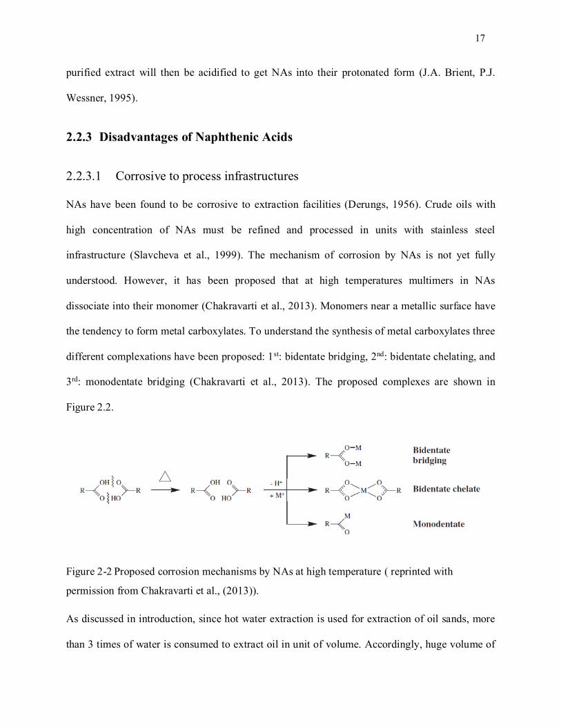
2.2.3.1 Corrosive to process infrastructures
NAs have been found to be corrosive to extraction facilities (Derungs, 1956). Crude oils with
high concentration of NAs must be refined and processed in units with stainless steel
infrastructure (Slavcheva et al., 1999). The mechanism of corrosion by NAs is not yet fully
understood. However, it has been proposed that at high temperatures multimers in NAs
dissociate into their monomer (Chakravarti et al., 2013). Monomers near a metallic surface have
the tendency to form metal carboxylates. To understand the synthesis of metal carboxylates three
different complexations have been proposed: 1st: bidentate bridging, 2nd: bidentate chelating, and
3rd: monodentate bridging (Chakravarti et al., 2013). The proposed complexes are shown in
Figure 2.2.
Figure 2-2 Proposed corrosion mechanisms by NAs at high temperature ( reprinted with
permission from Chakravarti et al., (2013)).
As discussed in introduction, since hot water extraction is used for extraction of oil sands, more
than 3 times of water is consumed to extract oil in unit of volume. Accordingly, huge volume of
18
water needs to be managed to reduce the environmental and financial cost of the process. The 80
to 85% water recycling rate greatly reduces the dependency of oil sands operations on fresh
water (Allen, 2008a). The disadvantage of the recycling process includes progressive
concentration of contaminants in the process affected water in tailings ponds (Allen, 2008a).
2.2.3.2 AEOs Toxicity
Research has demonstrated that NAs cause acute and chronic toxicity to a broad range of
organisms such as microorganisms, plants, birds, invertebrates and mammals (Headley and
McMartin, 2004; Kindzierski et al., 2012; Miskimmin et al., 2010). However, measuring NAs
concentration is insufficient for determining a relation between its concentration and toxicity
level (Clemente and Fedorak, 2005; Kindzierski et al., 2012). It is interesting that Headley and
McMartin (2004) discussed the contribution of surfactant behaviour of NAs to its toxicity. This
phenomenon called narcosis is where cell death (cell damage) occurs because of the entrance of
a hydrophobic compound into the lipid bilayer of cell membrane (Frank et al., 2009; Frank et al.,
2010; Tollefsen et al., 2012).
There are several extensive reviews on OSPW and NAs toxicity. As previously described,
OSPW has different portions of organics i.e. NAs and AEOs. For instance, AEOs represent the
acidic organics in the OSPW matrix. If toxicity tests are completed using AEOs, this procedure
neglects the other organics i.e. neutral organics. Recently, Morandi et al. (2015) conducted an
interesting experiment to study the contribution of different organics to acute toxicity of OSPW
(Morandi et al., 2015). The contribution of each portion was based on an extraction completed at
different pHs. They used two different toxicity tests a 96 h fathead minnow embryo lethality test
and a 15 min Microtox bioassay. Based on the results, the NAs (O2 -) are among the most
19
acutely toxic (organic) compounds in OSPW. However, nonacidic species (O+, O2+, SO+) also
cause acute toxicity (Morandi et al., 2015).
Since the AEOs and NAs are a complex group of compounds they are challenging to analyse.
The following section discusses the analysis of NAs where different instruments can give us a
different understanding of the system.
2.2.4 Quantification of Naphthenic Acids
Fourier Transform Infra-Red (FT-IR) has been utilized to analyse NAs and AEOs extensively for
academic and industrial purposes (Brown and Ulrich, 2015a; Jiveraj, 1995). Its popularity is due
to the fact that it is industries standard method for quantifying NAs. The instrument is user
friendly and analysis can be completed in a short time. In this method, a sample is first acidified
to a pH<2. To extract AEOs which contain NAs an extraction step is completed with an
appropriate organic solvent such as dichloromethane (Brown and Ulrich, 2015). During analysis
FTIR absorbance intensities of monomeric (single bond with a peak height of 1705 cm-1) and
dimeric (double bond with the peak height of 1743 cm-1) form of carboxylic groups ae summed
up to measure the concentration of NAs (Jiveraj, 1995). One should realize that FTIR has given
us the concentration of total carboxylic acids in a sample since it measures only the carboxyl
group.
Gas Chromatography is another technique used for AEOs measurements (Holowenko, 2002).
Samples after extraction need to be derivatized to transform NAs in AEOs to methyl esters. The
chromatogram results are shown as an unresolved hump (Brown and Ulrich, 2015). To analyse
the data, the integration of the hump is compared with the area of an internal standard.
20
Mass spectroscopy is one of the most common tools for NAs analysis. In this method one can
identify AEOs by plotting the relative response of each mass with respect to their n (number of
carbon) and Z (hydrogen deficiency) (Headley et al., 2013). Fig 2.2 illustrates the profile of
AEOs in OSPW. There are extensive reviews on the analysis of NAs with different resolution
techniques (Brown and Ulrich, 2015; Headley et al., 2013).
2.2.5 Treatment of OSPW and NAs contaminated wastewater
Based on aforementioned reasons, there is no doubt we need to remove NAs from waste streams. To have
a better understanding of available treatment technologies we will discuss both chemical and biological
treatments.
2.2.5.1 Chemical Treatment
Chemical treatment refers to the application of specific chemicals which react with a pollutant
and degrade them into environmentally safe end-products (Kabdasli and Arslan-Alaton, 2010). A
common practice is to use chemical oxidants which are a group of compounds that have high
redox potential (Siegrist et al., 2011). Oxidants accept electrons (from a pollutant in our case),
convert to their reduced form and leave the pollutant in an oxidized form. Organic pollutants
mainly exist in the reduced form of carbon where they have available electrons in their structure
(Tchobanoglous et al., 2003). To degrade reduced compounds they need to be oxidized. This
reaction happens by means of an oxidant. One question arises here! How can we know a given
compound can be an oxidant?
The general format of writing a redox reaction has been shown below (Bard and Faulkner, 2000):
Reduced compound + electron Oxidized compound
(2.1)
21
[Re + e- Ox]
Each half reaction has its own redox potential or cell potential that can be calculated based on
this formula (Bard and Faulkner, 2000):
E cell = E 0 cell - 𝑅𝑇
𝑛𝐹ln𝑄 (2.2)
E 0cell: is a standard cell potential at standard conditions (T= 25oC ; P= 1 atm; 1 molar
concentration) [V volt]
n: number of electrons transferred
R: ideal gas law constant (8.314 J mol-1 K-1)
F: Faraday constant (96500 J mol-1 V-1)
Q: reaction quotient
The reaction represents the ratio of products and reactants. For instance for a given reaction:
𝑎𝐴 + 𝑏𝐵 ↔ 𝑐𝐶 + 𝑑𝐷 (2.3)
The reaction quotient is:
𝑄 =𝐶𝐶
𝐶𝐶𝐷𝐷
𝐶𝐴𝑎𝐶𝐵
𝑏 (2.4)
Where equilibrium constant is:
𝐾𝑒𝑞 =𝐶𝐶,𝑒𝑞
𝐶 𝐶𝐷,𝑒𝑞𝐷
𝐶𝐴,𝑒𝑞𝑎 𝐶𝐵,𝑒𝑞
𝑏 (2.5)
Based on thermodynamic laws we know that for a spontaneous reaction to occur the Gibbs free
energy needs to be negative (∆G < 0). Gibbs free energy and redox potential are related as
follows (Bard and Faulkner, 2000):
∆G = - n F E0cell (2.6)
22
Based on this relationship when E0cell is positive, the Gibbs free energy is negative which means
accepting electrons can occur spontaneously. The higher the redox potential the stronger the
oxidant.
The three main things to consider when choosing a suitable oxidant for treatment purposes
include (Siegrist et al., 2011):
1. Stability in the environment
2. Selective reactivity to target pollutant
3. Redox potential of oxidant (oxidative power)
There are four commonly used oxidants in wastewater treatment based on chemical oxidation
(shown in Table 2-2).
Table 2-2 Common oxidants for chemical oxidation treatment goals (Siegrist et al., 2011).
Oxidant Chemical Formula Redox Potential (V)
Hydroxyl Radical HO-· 2.7
Sulfate Radical SO42-· 2.6
Ozone O3 2.2
Persulfate S2O82- 2.1
Hydrogen Peroxide H2O2 1.8
Permanganate MnO4- 1.7
Generally, advanced oxidation processes (AOPs) are more applicable and efficient than
oxidation processes (Oturan and Aaron, 2014). AOPs refer to an oxidation process with hydroxyl
radicals (HO·) (Oturan and Aaron, 2014). AOPs are more efficient because hydroxyl radicals are
very reactive to many organic pollutants and have high oxidizing power. There are different
ways to produce hydroxyl radicals, for example by activation of H2O2 by means of transitional
metal catalysts, UV light and ozone (Oturan and Aaron, 2014).
23
Due to the high degree of saturation in NAs they are a good candidate for treatment with
hydroxyl radicals (Andreozzi, 1999; Quinlan and Tam, 2015). Oxidation with HO· typically
occurs by hydrogen abstraction of the organics, in our case AEOs and NAs. The hydroxyl
radicals react with the NAs converting them to highly reactive organic radicals (Quinlan and
Tam, 2015). By progressing the oxidation reaction and propagation of the radical through the
organic compounds, complete degradation can be achieved. Complete oxidation (mineralization)
occurs when stable end products such as carbon dioxide, water and salts are produced.
Ozone (O3) is another favorable oxidant for the degradation of NAs (Andreozzi, 1999). Two
common ways to produce HO· with O3 is through alkaline pH or catalytic decomposition (Oturan
and Aaron, 2014). There is extensive research on ozonation of OSPW and elucidation of the
structure-reactivity relationship for NAs with ozone or H2O2/UV (Klamerth et al., 2015; Pérez-
Estrada et al., 2011; Scott et al., 2008; Wang et al., 2013b).
Other chemical approaches for treatment of NAs and OSPW have also been investigated. Mishra
et. al. (2010) studied the treatment of commercial NAs and AEOs in OSPW with microwave in
the presence of TiO2. An energy efficient method based on solar UV/chlorine advanced
oxidation process has also been reported (Shu et al., 2014). Using Gamma ray irradiation is one
of the newest technologies for removal of NAs and other organic contaminants ( Weisener et al.,
2013; Jia et al., 2015). Gamma rays electronically excite water molecules, which result in the
production of hydroxyl radicals and other molecules like hydrogen and hydrogen peroxide (Jia et
al., 2015). It is interesting to mention that so far Gamma ray irradiation has been environmentally
friendly, cost effective and high efficiency in removal of pollutants in lab scale research
(Weisener et al., 2013; Jia et al., 2015).
24
2.2.5.2 Biological Treatment
Bioremediation is an economical and effective technique for the degradation of organic
compounds. Bioremediation is based on the ability of microorganisms to consume organic
compounds as their source of energy and carbon. Microorganisms can take up soluble organic
components and leave carbon dioxide (in the case of complete mineralization), water, and new
biomass as the end products of their metabolism. Bioremediation techniques can use mixed
microbial cultures or pure cultures (Alexander, 1985; Alexander, 1999; Rittmann and McCarty,
2012; Tchobanoglous et al., 2003).
NAs are good candidates as biomarkers for oil source maturation because of their recalcitrance.
Used as a wood preservative (in the form of metal naphthenates) further indicates their resistance
to biological degradation. Recalcitrance does not mean the compounds cannot biologically
degrade at all. Sometimes these organic compounds are partially biodegradable. Biodegradation
of NAs was reported for the first time by Herman et al. (1994) (Herman et al., 1994). There are a
number of microorganisms that can grow on NAs, either model or mixture, in pure culture for
example Acinetobacter anitratum (Rho and Evans, 1975) , Alcaligenes faecalis (Blakley, 1974;
Whitby, 2010) and Pseudomonas putida (Blakley and Papish, 1982). There have been several
studies documenting the biodegradation of commercial NAs and AEOs in OSPW mainly under
aerobic conditions (Brown and Ulrich, 2015; Whitby, 2010). There is also an extensive review
on biodegradation of NAs (Clothier and Gieg, 2016; Whitby, 2010; Yue et al., 2015). One point
about biodegradation of NAs is the remaining presence of certain NAs in aged oil sands tailings
ponds that are resisting biodegradation. This fact confirms that NAs are partially biodegradable.
Natural attenuation, the process where indigenous microorganisms biodegrade organic
compounds in situ has been observed for NAs in tailings ponds. NAs with a high degree of
25
branching are shown to be more resistant to biodegradation by indigenous microorganisms.
Similar to AOPs (or any other case of bioremediation of specific organic compounds) there are
some relations between structure and biodegradation of NAs. For instance, aerobic batch
biotransformation assay with NAs enriched mixed culture has shown that NAs with a quaternary
carbon at the α- and β-position are non-biodegradable or have limited degree of
biotransformation (Misiti et al., 2014a). In biodegradation of 4-methyl-cyclohexane acetic acid
(C9H16O2), trans- isomers have higher (~2 times) biodegradation rate compare to cis- isomers
which shows the effect of alkyl side branching as one of the factors in biodegradability of NAs
(Huang et al., 2012). Results has shown that biodegradability of NAs decreases as side chain
increases (Johnson et al., 2011; Smith et al., 2008).
Approximately, the required time to achieve 50% biodegradation of commercial NAs strongly
depends on the Z number, which change from 1 to 8 days. A comparison of biodegradation of
commercial NAs and NAs in AEOs of OSPW can be seen in Fig 2-3.
26
Figure 2-3. Difference between biodegradation of commercial NAs and NAs in AEOs from
OSPW (reprinted with permission from Han et al (2008)).
Graph A shows the biodegradation of Merichem NAs where only 1.7% of NAs remains after 28
days of incubation. Graph B shows the biodegradation of NAs in AEOs in OSPW where 52% of
the initial concentration remains after 98 days of incubation. The remaining fraction is mostly
NAs with more rings and higher molecular weight. One of the reasons why commercial NAs are
more biodegradable than AEOs in OSPW is that commercial NAs are from petroleum sources
that have not undergone extensive biodegradation. NAs in OSPW (AEOs) have already
undergone biodegradation in tailings ponds. From a structural point of view, NAs in OSPW have
more alkyl chain branches and have more cyclic-compounds in their structure than commercial
NAs. These two properties are unfavorable from a biodegradation perspective.
Biodegradation of model NAs has also been conducted under anoxic conditions (Clothier and
Gieg, 2016; Dong and Nemati, 2016; Gunawan et al., 2014). Gunawan et al. (2014) studied the
27
biodegradation of trans-4-methyl-1-cyclohexane carboxylic under denitrifying conditions. Under
denitrificating conditions, NAs act as the electron donor and carbon source and nitrate acts as the
electron acceptor where it is reduced to N2 gas.
2.2.5.3 Coupling of Chemical and Biological Remediation
To optimize the removal of NAs and AEOs in OSPW the coupling of chemical (fast yet
expensive) and biological (slow yet affordable) treatment techniques is beneficial (Oller et al.,
2011). This concept is under development for the oil sands industry for treatment of OSPW.
Ozonation as a pre-treatment followed by aerobic biodegradation has shown an increase in
biodegradability of NAs as a result of ozonation pre-treatment (Brown et al., 2013; Martin et al.,
2010; Vaiopoulou et al., 2015). Based on Vaiopoulou et al.’s results, preferential degradation of
polycylclic and high molecular weight NAs by ozonation lead to a removal efficiency up to 89%.
Toxicity tests showed 15 times less toxic water as compared to untreated water (Vaiopoulou et
al., 2015).
One important point for consideration when coupling AOPs and biological remediation for in
situ remediation is the impact of the oxidant on the microorganisms. For in situ conditions a
pond will act as a reactor for both chemical oxidation and biological degradation. Strong
oxidants like ozone have been widely used as antimicrobial agents for disinfection purposes
(Camel and Bermond, 1998; Guzel-Seydim et al., 2004; Tchobanoglous et al., 2003). So how
will a mixed culture of microorganisms or a pure culture respond to the oxidation step in an in
situ application? For elucidating this phenomena we need to understand why oxidation pre-
treatment is harmful to microorganisms.
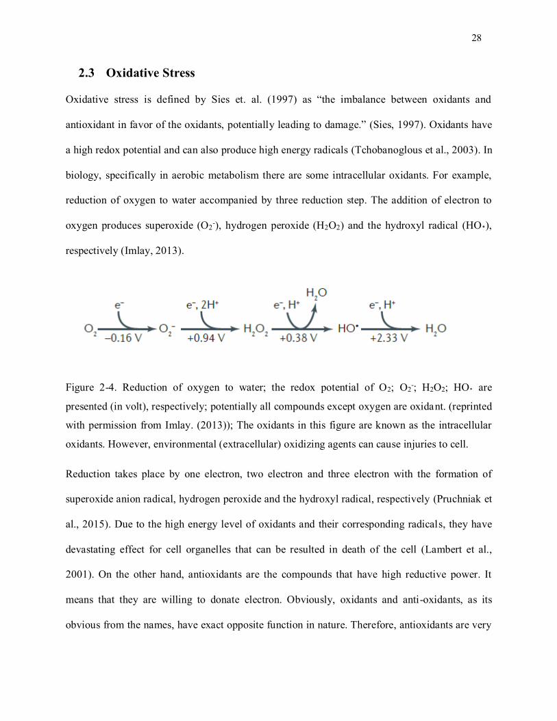
28
2.3 Oxidative Stress
Oxidative stress is defined by Sies et. al. (1997) as “the imbalance between oxidants and
antioxidant in favor of the oxidants, potentially leading to damage.” (Sies, 1997). Oxidants have
a high redox potential and can also produce high energy radicals (Tchobanoglous et al., 2003). In
biology, specifically in aerobic metabolism there are some intracellular oxidants. For example,
reduction of oxygen to water accompanied by three reduction step. The addition of electron to
oxygen produces superoxide (O2-), hydrogen peroxide (H2O2) and the hydroxyl radical (HO˖),
respectively (Imlay, 2013).
Figure 2-4. Reduction of oxygen to water; the redox potential of O2; O2-; H2O2; HO˖ are
presented (in volt), respectively; potentially all compounds except oxygen are oxidant. (reprinted
with permission from Imlay. (2013)); The oxidants in this figure are known as the intracellular
oxidants. However, environmental (extracellular) oxidizing agents can cause injuries to cell.
Reduction takes place by one electron, two electron and three electron with the formation of
superoxide anion radical, hydrogen peroxide and the hydroxyl radical, respectively (Pruchniak et
al., 2015). Due to the high energy level of oxidants and their corresponding radicals, they have
devastating effect for cell organelles that can be resulted in death of the cell (Lambert et al.,
2001). On the other hand, antioxidants are the compounds that have high reductive power. It
means that they are willing to donate electron. Obviously, oxidants and anti-oxidants, as its
obvious from the names, have exact opposite function in nature. Therefore, antioxidants are very
29
useful in neutralizing the oxidants by reducing their redox potential through accepting electrons.
Generally, an antioxidant is any compound, enzymatic or non-enzymatic, that can protect an
oxidizable substrate from being oxidized by an oxidant (Halliwell & Gutteridge, 2007).
Oxidative stress also happens through in vitro circumstances (Chapman, 2003). One such
example is the application of disinfectants like quaternary ammonium compounds, ozone, and
hypochlorite for disinfection purposes (Tezel and Pavlostathis, 2015;Stewart et al., 2001). The
disinfectant concentration is applied is in the order of hundreds to thousands times higher than
their minimum inhibitory concentration (MIC) (Andersson and Hughes, 2014). MIC is the
minimum concentration that prevents the observable growth of a given bacterial population
(Lambert et al., 2001;Andrews, 2001). Exposure of microbial populations to antimicrobial agents
below their MIC concentrations can have three different effects (Andersson and Hughes, 2014;
Lorian, 1975):
I. Selection of strategy for resistance (enrichment of resistant bacteria in
mixed cultures and selection of de novo methods)
II. Cause variation in genetic and phenotypic properties by enhancing the
ability for adaptive evolution and modification in resistance strategy
III. Change in physiological activities, biofilm formation or in general gene
expression
The last effect, variation in physiological properties or adaptive responses, is the main bridge
between environmental engineering goals and oxidative stress effect. In chapter 4 the impact
of oxidative stress due to persulfate on a Pseudomonas sp. will be determined.
30
2.4 Bioremediation Kinetics and Stoichiometry
When studying microbial growth kinetics (suspended cells) three different cultivation systems
are typically used: batch, continuous and fed-batch (Rittmann and McCarty, 2012). In batch
systems, the decrease in substrate concentration and increase in biomass is monitored over time
(Kristiansen, 1999; Rittmann and McCarty, 2012; Tchobanoglous et al., 2003). In continuous
systems the substrate and biomass concentration is constant over time (Kovarova-Kovar and
Egli, 1998). In other words, substrate and biomass concentration is time-dependent in a batch
system and time independent in a continuous system (Kovarova-Kovar and Egli, 1998). In
continuous systems (chemostat), microorganism(s) cultivate under stable environmental
condition i.e. dilution rate (Doran, 1995). Thus, in an ideal chemostat more precise, reproducible
and statistically relevant data can be obtained as compared to a batch system (steady state vs.
dynamic). However, data from a continuous system are not a good representation of growth
conditions found in nature. Generally, in a real environment microbial growth is best represented
somewhere between a closed system (batch) and open system (chemostat) (Kovarova-Kovar and
Egli, 1998).
There are two main concepts related to microbial growth: (1) nutrient limitation, and (2)
substrate limited growth. It should be noted that “limitation” refers to the stoichiometric aspects
of growth (since “limitation” indicates the amount or concentration!). Nutrient limitation is when
the nutrient amount becomes a decisive factor in biomass production. In other words, growth is a
function of the nutrient concentration. Secondly, substrate limited growth refers to the rate of
biosynthesis of new biomass governed by the specific substrate(s) concentration (Bailey, 1986;
Clark and Blanch, 1995; Kovarova-Kovar and Egli, 1998; Kristiansen, 1999).
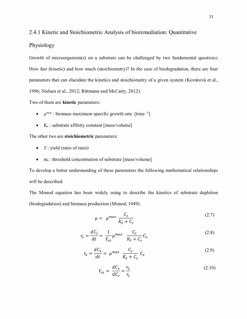
31
2.4.1 Kinetic and Stoichiometric Analysis of bioremediation: Quantitative
Physiology
Growth of microorganism(s) on a substrate can be challenged by two fundamental questions:
How fast (kinetic) and how much (stoichiometry)? In the case of biodegradation, there are four
parameters that can elucidate the kinetics and stoichiometry of a given system (Kovárová et al.,
1996; Nielsen et al., 2012; Rittmann and McCarty, 2012).
Two of them are kinetic parameters:
µmax : biomass maximum specific growth rate [time -1]
Ks : substrate affinity constant [mass/volume]
The other two are stoichiometric parameters:
Y : yield (ratio of rates)
ms : threshold concentration of substrate [mass/volume]
To develop a better understanding of these parameters the following mathematical relationships
will be described.
The Monod equation has been widely using to describe the kinetics of substrate depletion
(biodegradation) and biomass production (Monod, 1949).
µ = 𝜇𝑚𝑎𝑥 𝐶𝑠
𝐾𝑆 + 𝐶𝑠
(2.7)
𝑟𝑠 =𝑑𝐶𝑠
𝑑𝑡=
1
𝑌𝑠𝑥𝜇𝑚𝑎𝑥
𝐶𝑠
𝐾𝑆 + 𝐶𝑠
𝐶𝑥 (2.8)
𝑟𝑥 =𝑑𝐶𝑥
𝑑𝑡= 𝜇𝑚𝑎𝑥
𝐶𝑠
𝐾𝑆 + 𝐶𝑠 𝐶𝑥
(2.9)
𝑌𝑠𝑥 = 𝑑𝐶𝑥
𝑑𝐶𝑠=
𝑟𝑥
𝑟𝑠
(2.10)
32
In the above equations, 𝐶𝑠 substrate concentration and 𝐶𝑥 biomass concentration are dependent
variables and t time is an independent variable. µ is specific biomass growth rate which describes
the rate of biosynthesis of new cells per amount of present biomass (Bailey, 1986; Monod, 1949;
Nielsen et al., 2012; Rittmann and McCarty, 2012). Eq. 2.8 describes the rate of the substrate
consumption. It expresses how fast substrate is consumed in a bioreactor by means of
microorganisms. It can be seen that, 𝑟𝑠 has a direct relation to concentration of biomass.
However, in engineering working with independent parameters are more desirable. Because in
design problems or in analysis of a system, less parameters need to be considered, which is good!
In section 2.3.2 independent rates equation are described.
Eq. 2.10 expresses the yield of substrate to biomass. It shows the amount of substrate produced
per unit of consumed substrate. Logically, this amount (yield) can be obtained by diving the
rates. This parameter is one of the most important physiological parameter in design and analysis
of a biosystem. Because this parameter tells us the amount of biomass is produced in a bioreactor
and amount of biomass is very important in optimization purposes. Therefore, by knowing two
of the following quantities we can calculate another one: substrate consumption rate, biomass
production rate and yield. One should be realized that since yield is the ratio of two rates,
obtained results is independent of time. Since µ describes the rate of biomass production we can
correlate this expression to the doubling time td [time] of the cells.
𝑡𝑑 = ln 2
𝜇
(2.11)
Ks is the concentration of substrate where µ = 0.5 µmax. Ks can also be used as an affinity constant
of the substrate toward the cell (Kovárová et al., 1996; Kristiansen, 1999). Based on definition,
1/ Ks demonstrates the affinity of the cells to substrate.
33
A term not considered in the Monod model is ms, which is related to maintenance energy - the
amount of substrate cells need to survive at zero growth rate (Alexander, 1999; Kovarova-Kovar
and Egli, 1998; Kristiansen, 1999). Maintenance is also known as the amount of substrate needed
for endogenous metabolism and biosynthesis of new cells (Stephanopoulos et al., 1998). There
are other models, such as the Herbert-Pirt model (Pirt, 1965), which consider the maintenance
term when calculating the substrate uptake rate (Kristiansen, 1999; Nielsen et al., 2012;
Stephanopoulos et al., 1998). A detailed explanation of maintenance can be found in the
thermodynamic analysis section of this thesis (Section 5.4.1.1).
When the ratio between the consumed compounds and produced products are constant these
ratios are called stoichiometric coefficient or yield. In general, yields are the ratio of rates
(Kovarova-Kovar and Egli, 1998; Kristiansen, 1999; Rittmann and McCarty, 2012). One of the
most important yields in biodegradation processes is the ratio of produced biomass per consumed
substrate.
𝑌𝑆𝑋 =𝑎𝑚𝑜𝑢𝑛𝑡 𝑜𝑓 𝑏𝑖𝑜𝑚𝑎𝑠𝑠 𝑝𝑟𝑜𝑑𝑢𝑐𝑒𝑑
𝑎𝑚𝑜𝑢𝑛𝑡 𝑜𝑓 𝑠𝑢𝑠𝑏𝑡𝑟𝑎𝑡𝑒 𝑐𝑜𝑛𝑠𝑢𝑚𝑒𝑑
(2.12)
In general:
𝑌𝑖𝑗 =𝑎𝑚𝑜𝑢𝑛𝑡 𝑜𝑓 𝑗
𝑎𝑚𝑜𝑢𝑛𝑡 𝑜𝑓 𝑖=
𝑟𝑎𝑡𝑒𝑗
𝑟𝑎𝑡𝑒𝑖
(2.13)
2.4.2 Biomass Specific Rate: q-rate
In biological processes the substrate consumption rate is heavily dependent on the biomass
concentration. As such, it is important to quantify the rates per unit amount of biomass. To
overcome the dependency of the rates to the biomass concentration we can use the biomass
specific rate qi (Kristiansen, 1999; Smolke, 2009).
34
𝑞𝑖 = 𝑟𝑎𝑡𝑒𝑖
𝐶𝑥
(2.14)
These qi rates are very informative since we can easily track and then characterize the activity of
the cells (e.g. physiological parameters). qi rates are influenced by two factors (Smolke, 2009):
The cells: genotype effects such as genes, etc. [Genotype]
The environment of the cells: temperature, concentration of nutrient, etc. [Environment]
These q rates nicely represent the physiological properties of the cells (Nielsen et al., 2012;
Roels, 1983; Smolke, 2009; Stephanopoulos et al., 1998). It should be noted that qx which is a
biomass specific growth rate is equal to µ. q-rates are relevant and accurate for comparing of the
performance of two different systems (Boender et al., 2009; Smolke, 2009) . Similar to the
Monod model (hyperbolic model), qs (substrate specific uptake rate) can be described by a
hyperbolic function (Boender et al., 2009; Kristiansen, 1999; Van Loosdrecht and Henze, 1999).
𝑞𝑠 = 𝑞𝑠𝑚𝑎𝑥
𝐶𝑠
𝐾𝑠 + 𝐶𝑠
(2.15)
2.4.3 Biodegradation Thermodynamics
Generally, in engineering sciences one needs a combination of three concepts: kinetics (e.g.
transport phenomena, growth kinetics), balances (e.g. mass and energy balance) and equilibria
(e.g. force and phase equilibria) (von Stockar and van der Wielen, 1997). In environmental
biotechnology, balances and kinetics models have been extensively developed while
thermodynamic models have received little attention (Jaworska et al., 2002; Ramos et al., 2011;
Singh et al., 2008). A rough comparison shows that biological processes are not optimized as
much as chemical processes. This discrepancy can be attributed to a lack of fundamental
information. For example, mathematical models for deriving forces and energy efficiency and
35
position of thermodynamic equilibrium (and non-equilibrium state) do not exist (Urs von
Stockar, 2013).
2.4.3.1 Importance of Thermodynamics Analysis
When we complete a thermodynamic analysis, what can we find out and what can we do with the
results? Here are some of the possibilities (Heijnen, 1994; Kristiansen, 1999; Urs von Stockar,
2013):
Effect of temperature, pH, pressure, solutes and solvents on activity and selectivity
Correction of deriving force models for bioprocess design
Efficiency of cellular metabolism: optimal biomass and product yield
Thermodynamic effects in cellular growth including heat generation
Prediction of stoichiometric and kinetic parameters
Investigation of opportunities for novel product formation with a given substrate
Design of novel pathways for bioremediation purposes
Improvement of scale up approaches in bioprocesses
As it can be seen results from thermodynamic analysis are very informative specifically its
power in prediction of desired process parameters (Cueto-Rojas et al., 2015; Finley et al., 2010).
These possibilities are the main inspiration for investigating NAs biodegradation from a
thermodynamic perspective. More detailed discussions on this topic can be found in chapter five
of this thesis.
2.4.3.2 Thermodynamics of Naphthenic Acids biodegradation
Why Naphthenic Acids biodegradation is interesting for thermodynamic study?
36
When we are talking about biodegradation there are two very basic different cases to think about:
first is substrate (pollutant) and second one is microorganism. As we already knew NAs are
partially biodegradable. It means that microorganism cannot take up all substrate as source of
energy and carbon. The second topic that researchers can think is the ability of microorganisms
to remove NAs with focusing on the cell. And of course, we do not want to apply any changes in
substrate however, we are very interested in manipulation of the cells respect to our benefits.
Misiti et al. 2013 used thermodynamic analysis in their experiments for biodegradation of
commercial NAs under different electron accepting condition (Misiti et al., 2013; Misiti et al.,
2014b). However, the main points in thermodynamic analysis of bioremediation processes is
prediction of stoichiometry and kinetic parameters (von Stockar and van der Wielen, 1997)
which were not reported in their studies. Detailed related thermodynamics background is
described in chapter 5 of this thesis.
37
2.4 References
Abolfazlzadehdoshanbehbazari M, Birks SJ, Moncur MC, Ulrich AC. 2013. Fate and transport
of oil sand process-affected water into the underlying clay till: a field study. J. Contam.
Hydrol. 151:83–92.
Alexander M. 1985. Biodegradation of organic chemicals. Environ. Sci. Technol. 19:106–111.
Alexander M. 1999. Biodegradation and Bioremediation. Gulf Professional Publishing 453 p.
Allen EW. 2008a. Process water treatment in Canada’s oil sands industry: I. Target pollutants
and treatment objectives. J. Environ. Eng. Sci. 7:123–138.
Allen EW. 2008b. Process water treatment in Canada’s oil sands industry: II. A review of
emerging technologies. J. Environ. Eng. Sci. 7:499–524.
Andersson DI, Hughes D. 2014. Microbiological effects of sublethal levels of antibiotics. Nat.
Rev. Microbiol. 12:465–78.
Andreozzi R. 1999. Advanced oxidation processes (AOP) for water purification and recovery.
Catal. Today 53:51–59.
Andrews JM. 2001. Determination of minimum inhibitory concentrations. J. Antimicrob.
Chemother. 48:5–16.
Bailey JE. 1986. Biochemical Engineering Fundamentals. McGraw-Hill 984 p.
Bard AJ, Faulkner LR. 2000. Electrochemical Methods: Fundamentals and Applications, 2nd
Edition. John Wiley & Sons 856 p.
Blakley ER, Papish B. 1982. The metabolism of cyclohexanecarboxylic acid and 3-
cyclohexenecarboxylic acid by Pseudomonas putida. Can. J. Microbiol. 28:1324–9.
Blakley ER. 1974. The microbial degradation of cyclohexanecarboxylic acid: a pathway
involving aromatization to form p hydroxybenzoic acid. Can. J. Microbiol.
Boender LGM, de Hulster EAF, van Maris AJA, Daran-Lapujade PAS, Pronk JT. 2009.
Quantitative physiology of Saccharomyces cerevisiae at near-zero specific growth rates.
Appl. Environ. Microbiol. 75:5607–14.
Brown LD, Pérez-Estrada L, Wang N, El-Din MG, Martin JW, Fedorak PM, Ulrich AC. 2013.
Indigenous microbes survive in situ ozonation improving biodegradation of dissolved
organic matter in aged oil sands process-affected waters. Chemosphere 93:2748–55.
Brown LD, Ulrich AC. 2015. Oil sands naphthenic acids: a review of properties, measurement,
38
and treatment. Chemosphere 127:276–90.
Camel V, Bermond A. 1998. The use of ozone and associated oxidation processes in drinking
water treatment. Water Res. 32:3208–3222.
Chakravarti R, Patrick BN, Barney M, Kusinski G, Devine TM. 2013. Toward the Mechanism of
Corrosion in Crude Oil: A Study Using Vibrational Spectroscopic Techniques at Elevated
Temperatures. Energy & Fuels 27:7905–7914.
Chapman JS. 2003. Disinfectant resistance mechanisms, cross-resistance, and co-resistance. Int.
Biodeterior. Biodegradation 51:271–276.
Christopher Grant Weisener JJHC. 2013. Gamma Radiation Apparatus for Remediation of
Organic Compounds in Waste Slurries.
Clark DS, Blanch HW. 1995. Biochemical Engineering, Second Edition. CRC Press 702 p.
Clemente JS, Fedorak PM. 2005. A review of the occurrence, analyses, toxicity, and
biodegradation of naphthenic acids. Chemosphere 60:585–600.
Clothier LN, Gieg LM. 2016. Anaerobic biodegradation of surrogate naphthenic acids. Water
Res. 90:156–66.
Cueto-Rojas HF, van Maris AJA, Wahl SA, Heijnen JJ. 2015. Thermodynamics-based design of
microbial cell factories for anaerobic product formation. Trends Biotechnol. 33:534–46.
Derungs WA. 1956. Naphthenic Acid Corrosion —An Old Enemy Of the Petroleum Industry .
Corrosion 12:41–46.
Dong F, Nemati M. 2016. Anoxic biodegradation of a surrogate naphthenic acid coupled to
reduction of nitrite. Biochem. Eng. J.
Doran PM. 1995. Bioprocess Engineering Principles. Bioprocess Eng. Princ. Elsevier 426-439 p.
Finley SD, Broadbelt LJ, Hatzimanikatis V. 2010. In silico feasibility of novel biodegradation
pathways for 1,2,4-trichlorobenzene. BMC Syst. Biol. 4:7.
Frank RA, Sanderson H, Kavanagh R, Burnison BK, Headley J V, Solomon KR. 2010. Use of a
(quantitative) structure-activity relationship [(Q)SAR] model to predict the toxicity of
naphthenic acids. J. Toxicol. Environ. Health. A 73:319–29.
Frank RA, Fischer K, Kavanagh R, Burnison BK, Arsenault G, Headley J V., Peru KM, Kraak G
Van Der, Solomon KR. 2009. Effect of Carboxylic Acid Content on the Acute Toxicity of
Oil Sands Naphthenic Acids. Environ. Sci. Technol. 43:266–271.
Garcia-Garcia E, Ge JQ, Oladiran A, Montgomery B, El-Din MG, Perez-Estrada LC, Stafford
39
JL, Martin JW, Belosevic M. 2011. Ozone treatment ameliorates oil sands process water
toxicity to the mammalian immune system. Water Res. 45:5849–57.
Giesy JP, Anderson JC, Wiseman SB. 2010. Alberta oil sands development. Proc. Natl. Acad.
Sci. U. S. A. 107:951–2.
Government of Alberta. 2016. Oil sands quarterly. Open Text Web Site Management.
Grewer DM, Young RF, Whittal RM, Fedorak PM. 2010. Naphthenic acids and other acid-
extractables in water samples from Alberta: what is being measured? Sci. Total Environ.
408:5997–6010.
Gunawan Y, Nemati M, Dalai A. 2014. Biodegradation of a surrogate naphthenic acid under
denitrifying conditions. Water Res. 51:11–24.
Guzel-Seydim ZB, Greene AK, Seydim AC. 2004. Use of ozone in the food industry. LWT -
Food Sci. Technol. 37:453–460.
Halliwell B, Gutteridge JMC. 1985. Free radicals in biology and medicine.
Han X, Scott AC, Fedorak PM, Bataineh M, Martin JW. 2008. Influence of Molecular Structure
on the Biodegradability of Naphthenic Acids. Environ. Sci. Technol. 42:1290–1295.
Headley J V, Peru KM, Mohamed MH, Frank RA, Martin JW, Hazewinkel RRO, Humphries D,
Gurprasad NP, Hewitt LM, Muir DCG, Lindeman D, Strub R, Young RF, Grewer DM,
Whittal RM, Fedorak PM, Birkholz DA, Hindle R, Reisdorph R, Wang X, Kasperski KL,
Hamilton C, Woudneh M, Wang G, Loescher B, Farwell A, Dixon DG, Ross M, Pereira
ADS, King E, Barrow MP, Fahlman B, Bailey J, McMartin DW, Borchers CH, Ryan CH,
Toor NS, Gillis HM, Zuin L, Bickerton G, Mcmaster M, Sverko E, Shang D, Wilson LD,
Wrona FJ. 2013. Chemical fingerprinting of naphthenic acids and oil sands process waters-
A review of analytical methods for environmental samples. J. Environ. Sci. Health. A. Tox.
Hazard. Subst. Environ. Eng. 48:1145–63.
Headley J V, Peru KM, Barrow MP, Derrick PJ. 2007. Characterization of naphthenic acids from
athabasca oil sands using electrospray ionization: the significant influence of solvents. Anal.
Chem. 79:6222–9.
Headley J V., McMartin DW. 2004. A review of the occurrence and fate of naphthenic acids in
aquatic environments. J. Environ. Sci. Heal. - Part A Toxic/Hazardous Subst. Environ. Eng.
Headley J V., McMartin DW. 2007. A Review of the Occurrence and Fate of Naphthenic Acids
in Aquatic Environments. J. Environ. Sci. Heal. Part A.
40
Heijnen SJ. 1994. Thermodynamics of microbial growth and its implications for process design.
Trends Biotechnol. 12:483–492.
Herman DC, Fedorak PM, MacKinnon MD, Costerton JW. 1994. Biodegradation of naphthenic
acids by microbial populations indigenous to oil sands tailings. Can. J. Microbiol. 40:467–
477.
Holden AA, Haque SE, Mayer KU, Ulrich AC. 2013. Biogeochemical processes controlling the
mobility of major ions and trace metals in aquitard sediments beneath an oil sand tailing
pond: laboratory studies and reactive transport modeling. J. Contam. Hydrol. 151:55–67.
Holowenko F. 2002. Characterization of naphthenic acids in oil sands wastewaters by gas
chromatography-mass spectrometry. Water Res. 36:2843–2855.
Holowenko FM, MacKinnon MD, Fedorak PM. 2011. Methanogens and sulfate-reducing
bacteria in oil sands fine tailings waste. Can. J. Microbiol.
Huang J, Nemati M, Hill G, Headley J. 2012. Batch and continuous biodegradation of three
model naphthenic acids in a circulating packed-bed bioreactor. J. Hazard. Mater. 201-
202:132–40.
Imlay JA. 2013. The molecular mechanisms and physiological consequences of oxidative stress:
lessons from a model bacterium. Nat. Rev. Microbiol. 11:443–54.
Iranmanesh S, Harding T, Abedi J, Seyedeyn-Azad F, Layzell DB. 2014. Adsorption of
naphthenic acids on high surface area activated carbons. J. Environ. Sci. Health. A. Tox.
Hazard. Subst. Environ. Eng. 49:913–22.
J.A. Brient, P.J. Wessner MND. 1995. Kirk-Othmer Encyclopedia of Chemical Technology.
Hoboken, NJ, USA: John Wiley & Sons, Inc.
Jaworska J, Dimitrov S, Nikolova N, Mekenyan O. 2002. Probabilistic assessment of
biodegradability based on metabolic pathways: catabol system. SAR QSAR Environ. Res.
13:307–323.
Jia W, He Y, Ling Y, Hei D, Shan Q, Zhang Y, Li J. 2015. Radiation-induced degradation of
cyclohexanebutyric acid in aqueous solutions by gamma ray irradiation. Radiat. Phys.
Chem. 109:17–22.
Jiveraj MN. 1995. Naphthenic acids extraction and quantitative analy; fourth ed. Syncrude
Canada Ltd.; Research Department; Edmonton; AB.
Johnson RJ, Smith BE, Sutton PA, McGenity TJ, Rowland SJ, Whitby C. 2011. Microbial
41
biodegradation of aromatic alkanoic naphthenic acids is affected by the degree of alkyl side
chain branching. ISME J. 5:486–96.
Kabdasli I, Arslan-Alaton I. 2010. Chemical Oxidation Applications for Industrial Wastewaters.
IWA Publishing 341 p.
Kanicky JR, Poniatowski AF, Mehta NR, Shah DO. 2000. Cooperativity among Molecules at
Interfaces in Relation to Various Technological Processes: Effect of Chain Length on the p
K a of Fatty Acid Salt Solutions †. Langmuir 16:172–177.
Kannel PR, Gan TY. 2012. Naphthenic acids degradation and toxicity mitigation in tailings
wastewater systems and aquatic environments: a review. J. Environ. Sci. Health. A. Tox.
Hazard. Subst. Environ. Eng. 47:1–21.
Kindzierski W, Jin J, Gamal El-Din M. 2012. Review of Health Effects of Naphthenic Acids:
Data Gaps and Implications for Understanding Human Health Risk.
Klamerth N, Moreira J, Li C, Singh A, McPhedran KN, Chelme-Ayala P, Belosevic M, Gamal
El-Din M. 2015. Effect of ozonation on the naphthenic acids’ speciation and toxicity of pH -
dependent organic extracts of oil sands process-affected water. Sci. Total Environ. 506-
507:66–75.
Kovárová K, Zehnder AJ, Egli T. 1996. Temperature-dependent growth kinetics of Escherichia
coli ML 30 in glucose-limited continuous culture. J. Bacteriol. 178:4530–9.
Kovarova-Kovar K, Egli T. 1998. Growth Kinetics of Suspended Microbial Cells: From Single-
Substrate-Controlled Growth to Mixed-Substrate Kinetics. Microbiol. Mol. Biol. Rev.
62:646–666.
Kristiansen CRB. 1999, eds. Basic biotechnology. Cambridge University Press
Lambert RJW, Skandamis PN, Coote PJ, Nychas G-JE. 2001. A study of the minimum inhibitory
concentration and mode of action of oregano essential oil, thymol and carvacrol. J. Appl.
Microbiol. 91:453–462.
Lorian V. 1975. Some effects of subinhibitory concentrations of antibiotics on bacteria. Bull. N.
Y. Acad. Med. 51:1046–55.
Martin JW, Barri T, Han X, Fedorak PM, El-Din MG, Perez L, Scott AC, Jiang JT. 2010.
Ozonation of oil sands process-affected water accelerates microbial bioremediation.
Environ. Sci. Technol. 44:8350–6.
Misiti TM, Tezel U, Pavlostathis SG. 2014a. Effect of alkyl side chain location and cyclicity on
42
the aerobic biotransformation of naphthenic acids. Environ. Sci. Technol. 48:7909–17.
Misiti T, Tandukar M, Tezel U, Pavlostathis SG. 2013. Inhibition and biotransformation
potential of naphthenic acids under different electron accepting conditions. Water Res.
47:406–18.
Misiti T, Tandukar M, Tezel U, Pavlostathis SG. 2014b. Corrigendum to “Inhibition and
biotransformation potential of naphthenic acids under different electron accepting
conditions” [Water Res. 47 (1) (January 2013) 406–418]. Water Res. 48:645.
Miskimmin, B., Fedorak P., Lauman R. & VK. 2010. Oil sands water toxicity: A critical review.
Monod J. 1949. The Growth of Bacterial Cultures. Annu. Rev. Microbiol. 3:371–394.
Morandi GD, Wiseman SB, Pereira A, Mankidy R, Gault IGM, Martin JW, Giesy JP. 2015.
Effects-Directed Analysis of Dissolved Organic Compounds in Oil Sands Process-Affected
Water. Environ. Sci. Technol. 49:12395–404.
Nielsen J, Villadsen J, Lidén G. 2012. Bioreaction Engineering Principles: Second Edition.
Springer 528 p.
Oller I, Malato S, Sánchez-Pérez JA. 2011. Combination of Advanced Oxidation Processes and
biological treatments for wastewater decontamination--a review. Sci. Total Environ.
409:4141–66.
Oturan MA, Aaron J-J. 2014. Advanced Oxidation Processes in Water/Wastewater Treatment:
Principles and Applications. A Review. Crit. Rev. Environ. Sci. Technol. 44:2577–2641.
Pérez-Estrada LA, Han X, Drzewicz P, Gamal El-Din M, Fedorak PM, Martin JW. 2011.
Structure-reactivity of naphthenic acids in the ozonation process. Environ. Sci. Technol.
45:7431–7.
Pirt SJ. 1965. The Maintenance Energy of Bacteria in Growing Cultures. Proc. R. Soc. B Biol.
Sci. 163:224–231.
Pruchniak MP, Araźna M, Demkow U. 2015. Biochemistry of Oxidative Stress. Adv. Exp. Med.
Biol.
Quagraine EK, Peterson HG, Headley J V. 2005. In Situ Bioremediation of Naphthenic Acids
Contaminated Tailing Pond Waters in the Athabasca Oil Sands Region—Demonstrated
Field Studies and Plausible Options: A Review. J. Environ. Sci. Heal. Part A 40:685–722.
Quinlan PJ, Tam KC. 2015. Water treatment technologies for the remediation of naphthenic
acids in oil sands process-affected water. Chem. Eng. J. 279:696–714.
43
Ramos J-L, Marqués S, van Dillewijn P, Espinosa-Urgel M, Segura A, Duque E, Krell T,
Ramos-González M-I, Bursakov S, Roca A, Solano J, Fernádez M, Niqui JL, Pizarro-
Tobias P, Wittich R-M. 2011. Laboratory research aimed at closing the gaps in microbial
bioremediation. Trends Biotechnol. 29:641–7.
Rho EM, Evans WC. 1975. The aerobic metabolism of cyclohexanecarboxylic acid by
Acinetobacter anitratum. Biochem. J. 148:11–15.
Rittmann B, McCarty P. 2012. Environmental biotechnology: principles and applications.
Roels JA. 1983. Energetics and kinetics in biotechnology.
Rogers V V. 2002. Acute and Subchronic Mammalian Toxicity of Naphthenic Acids from Oil
Sands Tailings. Toxicol. Sci. 66:347–355.
Ross MS, Pereira A dos S, Fennell J, Davies M, Johnson J, Sliva L, Martin JW. 2012.
Quantitative and qualitative analysis of naphthenic acids in natural waters surrounding the
Canadian oil sands industry. Environ. Sci. Technol. 46:12796–805.
Scott AC, Zubot W, MacKinnon MD, Smith DW, Fedorak PM. 2008. Ozonation of oil sands
process water removes naphthenic acids and toxicity. Chemosphere 71:156–60.
Shu Z, Li C, Belosevic M, Bolton JR, El-Din MG. 2014. Application of a solar UV/chlorine
advanced oxidation process to oil sands process-affected water remediation. Environ. Sci.
Technol. 48:9692–701.
Siegrist R, Crimi M, Simpkin T. 2011. In situ chemical oxidation for groundwater remediation.
Sies H. 1997. Oxidative stress: oxidants and antioxidants. Exp. Physiol. 82:291–295.
Singh S, Kang SH, Mulchandani A, Chen W. 2008. Bioremediation: environmental clean-up
through pathway engineering. Curr. Opin. Biotechnol. 19:437–44.
Slavcheva E, Shone B, Turnbull A. 1999. Review of naphthenic acid corrosion in oilrefining. Br.
Corros. J. 34:125–131.
Smith BE, Lewis CA, Belt ST, Whitby C, Rowland SJ. 2008. Effects of Alkyl Chain Branching
on the Biotransformation of Naphthenic Acids. Environ. Sci. Technol. 42:9323–9328.
Smolke C. 2009. The Metabolic Pathway Engineering Handbook: Fundamentals. CRC Press 678
p.
Stephanopoulos G, Aristidou AA, Nielsen J. 1998. Metabolic Engineering: Principles and
Methodologies. Academic Press 725 p.
Stewart PS, Rayner J, Roe F, Rees WM. 2001. Biofilm penetration and disinfection efficacy of
44
alkaline hypochlorite and chlorosulfamates. J. Appl. Microbiol. 91:525–532.
von Stockar U, van der Wielen LAM. 1997. Thermodynamics in biochemical engineering. J.
Biotechnol. 59:25–37.
Tchobanoglous G, Burton FL, Stensel HD, Eddy M&. 2003. Wastewater Engineering: Treatment
and Reuse. McGraw-Hill Education 1819 p.
Tezel U, Pavlostathis SG. 2015. Quaternary ammonium disinfectants: microbial adaptation,
degradation and ecology. Curr. Opin. Biotechnol. 33:296–304.
Tollefsen KE, Petersen K, Rowland SJ. 2012. Toxicity of synthetic naphthenic acids and
mixtures of these to fish liver cells. Environ. Sci. Technol. 46:5143–50.
Urs von Stockar LAM van der W. 2013. Biothermodynamics: The Role of Thermodynamics in
Biochemical Engineering. https://www.crcpress.com/Biothermodynamics-The-Role-of-
Thermodynamics-in-Biochemical-Engineering/Stockar-van-der-Wielen/9781466582163.
Vaiopoulou E, Misiti TM, Pavlostathis SG. 2015. Removal and toxicity reduction of naphthenic
acids by ozonation and combined ozonation-aerobic biodegradation. Bioresour. Technol.
179:339–47.
VANLOOSDRECHT M, HENZE M. 1999. Maintenance, endogeneous respiration, lysis, decay
and predation. Water Sci. Technol. 39:107–117.
Wang N, Chelme-Ayala P, Perez-Estrada L, Garcia-Garcia E, Pun J, Martin JW, Belosevic M,
Gamal El-Din M. 2013a. Impact of ozonation on naphthenic acids speciation and toxicity of
oil sands process-affected water to Vibrio fischeri and mammalian immune system.
Environ. Sci. Technol. 47:6518–26.
Wang N, Chelme-Ayala P, Perez-Estrada L, Garcia-Garcia E, Pun J, Martin JW, Belosevic M,
Gamal El-Din M. 2013b. Impact of ozonation on naphthenic acids speciation and toxicity of
oil sands process-affected water to Vibrio fischeri and mammalian immune system.
Environ. Sci. Technol. 47:6518–26.
Whitby C. 2010. Microbial naphthenic Acid degradation. Adv. Appl. Microbiol. 70:93–125.
Yue S, Ramsay BA, Ramsay JA. 2015. Biodegradation of naphthenic acid surrogates by axenic
cultures. Biodegradation 26:313–25.
45
CHAPTER 3. STOICHIOMETRIC DETERMINATION OF
PERSULFATE DOSES FOR OXIDATION OF ACID
EXTRACTABLE ORGANICS
3.1 Introduction
One of the largest industrial activities in the world is bitumen mining activities in the Alberta oil
sands deposits (Leshuk et al., 2016). Due to the alkaline hot water process for extraction of
surface-mined bitumen, large volumes of oil sands process affected water (OSPW) are produced.
The extraction process produces 1.25 m3 of tailings per barrel of produced oil and more than
three liters of water will be consumed ( 𝑐𝑜𝑛𝑠𝑢𝑚𝑒𝑑 𝑤𝑎𝑡𝑒𝑟
𝑝𝑟𝑜𝑑𝑢𝑐𝑒𝑑 𝑜𝑖𝑙 > 3) in the production of one liter of oil
(Allen, 2008a; Government of Alberta, 2016). The zero discharge policy and lack of an
established treatment strategy (for treatment of OSPW) results in the storage of OSPW in on-site
tailings ponds (Government of Alberta, 2016). OSPW consists of different compounds i.e.
suspended clays, dissolved organic compounds, trace heavy metals, and residual bitumen (Allen,
2008). Efforts in developing OSPW treatment methods have shown that naphthenic acids (NAs)
are the most important compounds that need to be removed from OSPW (Allen, 2008; Brown
and Ulrich, 2015; Clemente and Fedorak, 2005) due to their contribution in toxicity of OSPW
(Garcia-Garcia et al., 2011; He et al., 2012; Marentette et al., 2015; Miskimmin, B., Fedorak P.,
Lauman R., 2010; Shu et al., 2014; Wang et al., 2013) and its corrsoivity to process instruments
and vessels (Chakravarti et al., 2013; Derungs, 1956; Slavcheva et al., 1999).
NAs are naturally occurring compounds found in crude oil. They are a complicated mixture of
carboxylic acids which are generally shown by the formula CnH2n+zO2. In this formula ‘n’
represents carbon number, while ‘z’ represents the number of cycles in the NA structure
46
(Clemente and Fedorak, 2005). NAs concentration in OSPW may differ based on the source of
crude oil, the age of the tailings ponds, and the process used in extraction (Allen, 2008a;
Clemente and Fedorak, 2005; Headley and McMartin, 2004).
Naturally occurring NAs found in OSPW are just a portion of bigger group of organics called
acid extractable organics (AEOs) (Grewer et al., 2010). The acid term comes from the process
for extraction of this group of organics where a sample is acidified to pH<2 to have the acidic
constituents of OSPW matrix in their protonated form (Brown and Ulrich, 2015). After the
extraction with an organic solvent, the obtained complex mix of organic compounds are termed
AEOs. Characterizations with high resolution techniques have determined that NAs are a
fraction of these OSPW sourced AEOs (Grewer et al., 2010).
The use of chemical oxidants for treatment of industrial wastewatesr has always been of interest
(Kabdasli and Arslan-Alaton, 2010; Oturan and Aaron, 2014). Some examples include the use of
ozone for treatment of pharmaceutical wastewater and hydrogen peroxide for removal of micro
pollutants in wastewater (Rice, 1996; Robinson et al., 2001). Oxidants are chemical compounds
that have a high tendency to accept electrons. There are number of oxidants that can be used for
remediation purposes, such as permanganate and persulfate (Kabdasli and Arslan-Alaton, 2010).
The applicability of an oxidant depends on many factors such as: is the oxidant reactive toward
the target compound? If yes, how much do we need to meet the pre-defined treatment
requirements? Or how fast can the oxidant remove the pollutant?
Sodium persulfate with a redox potential of +2.01 V is one the newest oxidants used for
remediation purposes (Liu et al., 2014; Tsitonaki et al., 2010). The persulfate ion reduces to
sulfate by accepting two electrons based on following reaction (Tsitonaki et al., 2010):
47
𝑆2𝑂82− + 2𝑒− → 2𝑆𝑂4
2− ; 𝐸0 = +2.01 𝑉 (3.1)
However, the use of persulfate as an oxidant may have some unfavorable consequences, such as
a decrease in pH of the contaminated aqueous phase to acidic levels (depends on the buffer
capacity of the aquifer) (Huang et al., 2002; Liang et al., 2004) and a change in the redox regime
of the treated area (Sutton et al., 2014). Production of sulfate as the reduced form of persulfate
can stimulate the activity of sulfate reducing bacteria (SRB) since they use sulfate as their
terminal electron acceptor (Muyzer and Stams, 2008). In SRB’s metabolism, sulfate will be
reduced to sulfide (S2-) which can also create potential environmental concerns (Muyzer and
Stams, 2008). For example, in tailings ponds an increase in hydrogen sulfide emissions, which is
a toxic gas, has been observed (Holowenko et al., 2011; Ramos-Padrón et al., 2011). Therefore,
the concentration of persulfate should be as low as possible to minimize secondary
environmental issues.
The persulfate ion has shown to be reactive toward oxidation of NAs in OSPW (Drzewicz et al.,
2012; Sohrabi et al., 2013). Sohrabi et al. (2013) used 10 g/L of unactivated sodium persulfate
for removal of NAs in OSPW. To demonstrate the degradation of NAs over time, Sohrabi et al.
(2010) measured the concentration of total carboxylic acids. Results demonstrate that almost
complete removal of carboxylic acids was achieved after 111 days (Sohrabi et al., 2013).
However, there was no discussion about the actual and/or needed amout of persulfate for
treatment of NAs.
As previously mentioned, determining a stiochiometric amount of oxidant needed to react with
the contaminant of concern is one of the main factors in designing and optimizing a remediation
process. However, this process is challenging when dealing with NAs since they consist of a
mixture containing thousands of complex organic compounds. Additionally, current analytical
48
techniques are semi-quantitative in nature due to the complexity of the mixture (Brown and
Ulrich, 2015; Clemente et al., 2003; Headley et al., 2007; Holowenko, 2002). Previous lab-scale
research has shown success in using oxidants in treating NAs in an OSPW matrix (Brown and
Ulrich, 2015; Quinlan and Tam, 2015). However, there is no current strategy proposed for
determining the practical dosage of oxidants that are needed for an industrial application.
Currently, there is a lack of a simple, cost effective and practical protocol for determination of
oxidant doses needed for removal of NAs in OSPW or NAs contaminated wastewater. This
knowledge gap provides the authors with an opportunity to develop a simple model to
approximately predict the amount of needed persulfate (oxidant) for remediation purposes.
3.2 Materials and Methods
3.2.1 Chemicals and Material Preparation
Sodium persulfate (≥99%) was purchased from Sigma Aldrich. Methylene chloride (DCM)
HPLC grade (99.9 % min_Scientific Fischer) was used as the organic solvent to extract AEOs
from OSPW. Merichem NAs (Merichem Chemicals and Refinery Service, Houston, TX) was
used as the calibration standard. All chemicals were certified A.C.S and all solutions were
prepared in glass made containers.
Syncrude Mildred Lake settling basin (MLSB) tailings pond water was used as the source of
OSPW. MLSB OSPW was filtered through a 0.22 µm (Milipore) nylon filter to eliminate
microbial and solid state material in the liquid phase.
49
3.2.2 Kinetic Experiments
Experiments were performed using four different dosages of persulfate oxidant with respect to
the predicted stoichiometric amount (D) – 0.25D, 0.5D, D, 2D. Sodium persulfate was dissolved
in 500 mL OSPW contained in 1 L capped amber bottles. Magnetic stir bars were used to
continuously mix the contents at room temperature.
3.2.3 Analytical Methods
Chemical oxygen demand (COD) of MLSB OSPW was measured with HACH COD digestion
vials using a HACH thermoreactor and spectrophometer. To analyze the NAs in OSPW we first
need to extract AEOs as per the following protocol:
Samples were immediately acidified to pH < 2 by addition of concentrated HCl. The purpose of
acidification is to convert acidic contents to their protonated form. Then DCM was added to
samples to transfer organic acids into the organic phase. The extraction step was repeated 5 times
for extraction of AEOs from each sample and conducted in triplicate. One should note that by
increasing the number of extraction steps better extraction efficiency can be obtained instead of
using high volume of solvent.
Analysis of NAs in AEOs was performed by Fourier transform infrared (FTIR) spectroscopy
over the time course of the reaction (Jiveraj, 1995). When using FTIR as an analytical technique
one measures the concentration of total carboxylic acids. Standards were prepared
gravimetrically using a known concentration of Merichem NAs in DCM. FTIR spectroscopy was
performed using a PerkinElmer® Spectrum 100 instrument and PerkinElmer® Spectrum 10
software (Perkin Elmer, Waltham, MA). A FTIR cell with potassium bromide window, 3 mm-
spaced (University of Alberta, Edmonton, AB) was used in the spectroscopy runs. Summation of
50
peak heights for monomers hydrogen-bond dimers, 1743 and 1705 cm-1 respectively were used
in calculating the total NAs (AEOs) concentration. Each sample was extracted and ran in
triplicate with 32 scans (Brown et al., 2013; Mahdavi et al., 2015).
3.3 Results and Discussion
3.3.1 Fundamentals of Proposed Model
This model is based on the concept of chemical oxygen demand (COD). COD is a concentration
that determines the amount of oxygen needed to oxidize organic compounds in a mixture. In the
proposed model, the assumption was all the COD originating from the concentration of NAs.
The advantages of this assumption is contribution of other organic pollutants i.e. benzene,
toluene, ethylbenzen and xylene or polycyclic aromatic compounds are also considered. As all of
the organics contribute to COD of the solution, the estimated dosages is actually for treatment of
all organics in the solution. This is applicable to a complex mixture of organic compounds just as
is the case for NAs in OSPW. Since COD has units of 𝑚𝑎𝑠𝑠
𝑣𝑜𝑙𝑢𝑚𝑒 that relate to
𝑚𝑎𝑠𝑠 𝑜𝑓 𝑂2
𝑣𝑜𝑙𝑢𝑚𝑒 𝑜𝑓 𝑙𝑖𝑞𝑢𝑖𝑑 one
can measure the COD of a sample to get an idea of available electrons for oxidation (van
Loosdrecht et al., 2016; Rittmann and McCarty, 2012).
Based on the half reaction of oxygen (Rittmann and McCarty, 2012):
𝑂2 + 4𝑒− + 4𝐻+ → 2 𝐻2𝑂 ; 𝐸0 = +1.23 𝑉 (3.2)
1 mole of O2 accepts 4 moles of electrons (degree of reduction of oxygen = -4), which can be
also expressed as 32 g of O2 accepts 4 moles of electrons or as 32 gCOD accepts 4 moles of
electrons. Or in its simplest form of 8 gCOD accepts 1 mole of electrons. For instance, for a
wastewater with COD of 500 mg/L one can calculate the available electrons as follows on a per
1L basis:
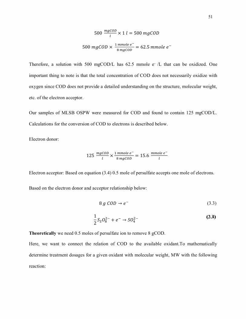
51
4 500 𝑚𝑔𝐶𝑂𝐷
𝑙× 1 𝑙 = 500 𝑚𝑔𝐶𝑂𝐷
5 500 𝑚𝑔𝐶𝑂𝐷 × 1 𝑚𝑚𝑜𝑙𝑒 𝑒−
8 𝑚𝑔𝐶𝑂𝐷= 62.5 𝑚𝑚𝑜𝑙𝑒 𝑒−
Therefore, a solution with 500 mgCOD/L has 62.5 mmole e- /L that can be oxidized. One
important thing to note is that the total concentration of COD does not necessarily oxidize with
oxygen since COD does not provide a detailed understanding on the structure, molecular weight,
etc. of the electron acceptor.
Our samples of MLSB OSPW were measured for COD and found to contain 125 mgCOD/L.
Calculations for the conversion of COD to electrons is described below.
Electron donor:
6 125 𝑚𝑔𝐶𝑂𝐷
𝑙×
1 𝑚𝑚𝑜𝑙𝑒 𝑒−
8 𝑚𝑔𝐶𝑂𝐷= 15.6
𝑚𝑚𝑜𝑙𝑒 𝑒−
𝑙
Electron acceptor: Based on equation (3.4) 0.5 mole of persulfate accepts one mole of electrons.
Based on the electron donor and acceptor relationship below:
8 𝑔 𝐶𝑂𝐷 → 𝑒− (3.3)
1
2𝑆2𝑂8
2− + 𝑒− → 𝑆𝑂42−
(2.3)
(3.4)
Theoretically we need 0.5 moles of persulfate ion to remove 8 gCOD.
Here, we want to connect the relation of COD to the available oxidant.To mathematically
determine treatment dosages for a given oxidant with molecular weight, MW with the following
reaction:
52
𝑂𝑥 + 𝑛𝑒− → 𝑅𝑒𝑑 (3.5)
𝑡ℎ𝑒𝑜𝑟𝑒𝑡𝑖𝑐𝑎𝑙 𝑑𝑜𝑠𝑎𝑔𝑒 𝑜𝑓 𝑛𝑒𝑒𝑑𝑒𝑑 𝑜𝑥𝑖𝑑𝑎𝑛𝑡 𝐷 [𝑔 𝑜𝑥
𝑙] =
𝐶𝑂𝐷 [𝑔 𝐶𝑂𝐷
𝑙] × 𝑀𝑊 [
𝑔 𝑜𝑥𝑚𝑜𝑙 𝑜𝑥
]
8 [𝑔 𝐶𝑂𝐷𝑚𝑜𝑙 𝑒−] × 𝑛 [
𝑚𝑜𝑙 𝑒−
𝑚𝑜𝑙 𝑜𝑥]
(3.6)
Specifically, for the sodium persulfate ion we can calculcate the dose (D) as follows:
𝐷 = 𝐶𝑂𝐷 × 238
8 × 2
(3.7)
3.3.2 Determination of Required Dosage of Oxidant
COD of MLSB OSPW was measured as 125 mg/L. Based on the proposed model, one can
determine the stoichiometrically needed dosage of persulfate (D) to be 1.86 g/L for sodium salt
of persulfate. Calculation of obtained result is described below:
𝐷 =125 [
𝑚𝑔 𝐶𝑂𝐷𝑙
] × 238 [𝑚𝑔 𝑁𝑎2𝑆2𝑂8
𝑚𝑚𝑜𝑙 𝑁𝑎2𝑆2𝑂8]
8 [𝑚𝑔 𝐶𝑂𝐷𝑚𝑚𝑜𝑙 𝑒−] × 2 [
𝑚𝑚𝑜𝑙 𝑒−
𝑚𝑚𝑜𝑙 𝑁𝑎2𝑆2𝑂8]
= 1860 [𝑚𝑔 𝑁𝑎2𝑆2𝑂8
𝑙] = 1.86 [
𝑔 𝑁𝑎2𝑆2𝑂8
𝑙]
Theoretically, this amount of persulfate can oxidize all organic electron donors in OSPW. To test
the ability of persulfate to oxidize the COD in OSPW. However, our target in this work is to
oxidize NAs. In measurement of COD, all the organic pollutants are considered, and a fraction of
measured organics are NAs. Therefore, we tested oxidant doses ranging from lower predicted
dosage to higher. Dosages are 0.25, 0.5, 1 and 2 times of the theoretical calculated value (D),
which correspond to actual concentrations of 0.47, 0.93, 1.86 and 3.72 g/L of sodium persulfate.
The concentration of total carboxylic acids was monitored over a 28 day period as shown in Fig
3-1.
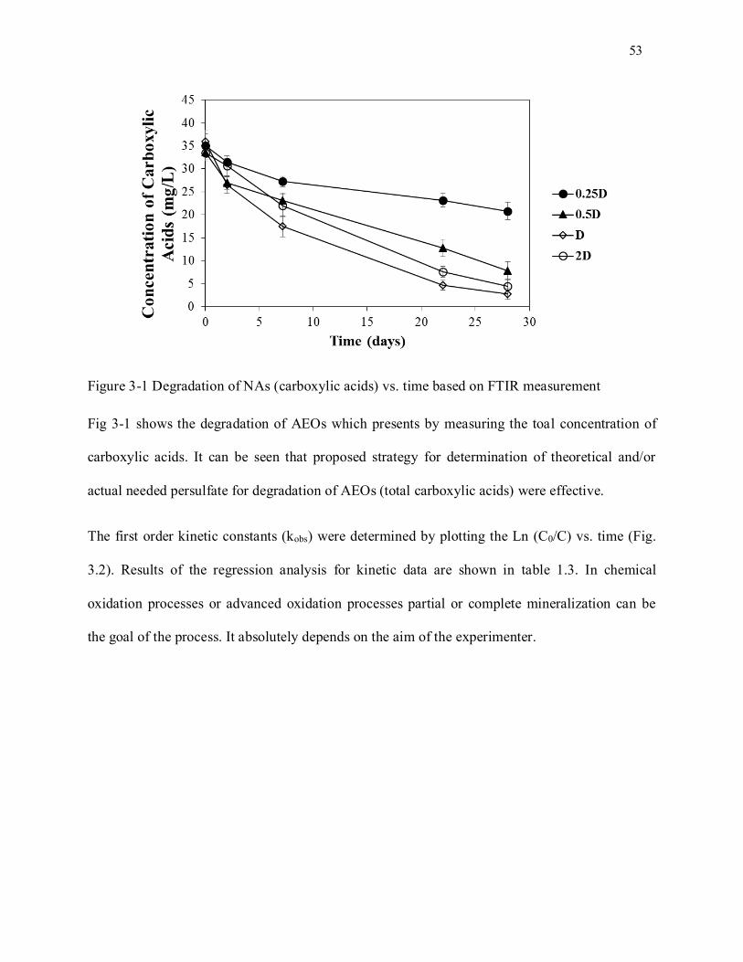
53
Figure 3-1 Degradation of NAs (carboxylic acids) vs. time based on FTIR measurement
Fig 3-1 shows the degradation of AEOs which presents by measuring the toal concentration of
carboxylic acids. It can be seen that proposed strategy for determination of theoretical and/or
actual needed persulfate for degradation of AEOs (total carboxylic acids) were effective.
The first order kinetic constants (kobs) were determined by plotting the Ln (C0/C) vs. time (Fig.
3.2). Results of the regression analysis for kinetic data are shown in table 1.3. In chemical
oxidation processes or advanced oxidation processes partial or complete mineralization can be
the goal of the process. It absolutely depends on the aim of the experimenter.
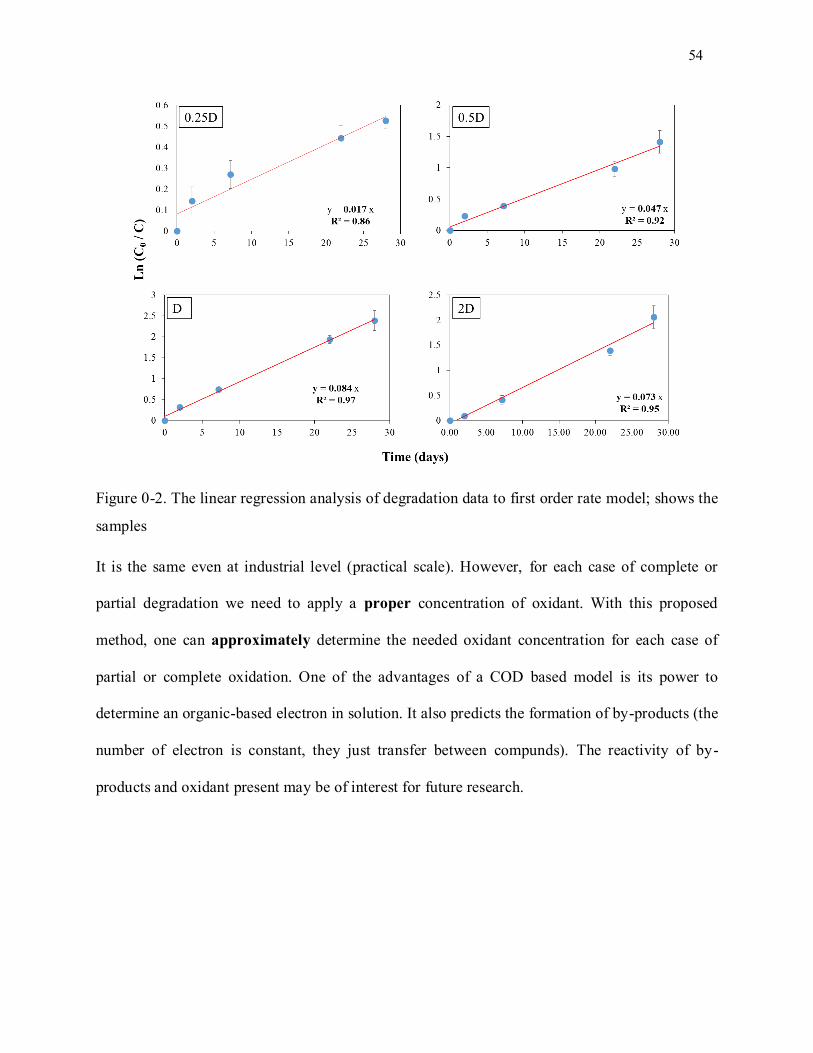
54
Figure 0-2. The linear regression analysis of degradation data to first order rate model; shows the
samples
It is the same even at industrial level (practical scale). However, for each case of complete or
partial degradation we need to apply a proper concentration of oxidant. With this proposed
method, one can approximately determine the needed oxidant concentration for each case of
partial or complete oxidation. One of the advantages of a COD based model is its power to
determine an organic-based electron in solution. It also predicts the formation of by-products (the
number of electron is constant, they just transfer between compunds). The reactivity of by-
products and oxidant present may be of interest for future research.
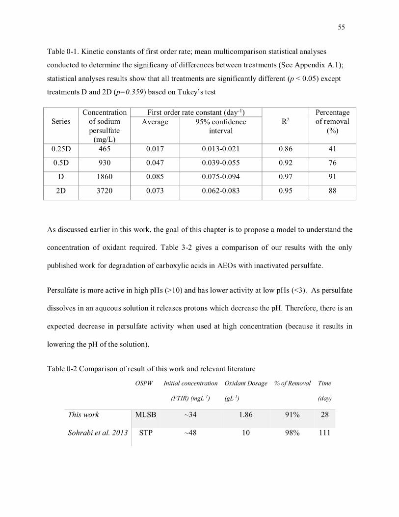
55
Table 0-1. Kinetic constants of first order rate; mean multicomparison statistical analyses
conducted to determine the significany of differences between treatments (See Appendix A.1);
statistical analyses results show that all treatments are significantly different (p < 0.05) except
treatments D and 2D (p=0.359) based on Tukey’s test
Series
Concentration
of sodium
persulfate
(mg/L)
First order rate constant (day-1)
R2
Percentage
of removal
(%)
Average 95% confidence
interval
0.25D 465 0.017 0.013-0.021 0.86 41
0.5D 930 0.047 0.039-0.055 0.92 76
D 1860 0.085 0.075-0.094 0.97 91
2D 3720 0.073 0.062-0.083 0.95 88
As discussed earlier in this work, the goal of this chapter is to propose a model to understand the
concentration of oxidant required. Table 3-2 gives a comparison of our results with the only
published work for degradation of carboxylic acids in AEOs with inactivated persulfate.
Persulfate is more active in high pHs (>10) and has lower activity at low pHs (<3). As persulfate
dissolves in an aqueous solution it releases protons which decrease the pH. Therefore, there is an
expected decrease in persulfate activity when used at high concentration (because it results in
lowering the pH of the solution).
Table 0-2 Comparison of result of this work and relevant literature
OSPW Initial concentration
(FTIR) (mgL-1)
Oxidant Dosage
(gL-1)
% of Removal Time
(day)
This work MLSB ~34 1.86 91% 28
Sohrabi et al. 2013 STP ~48 10 98% 111
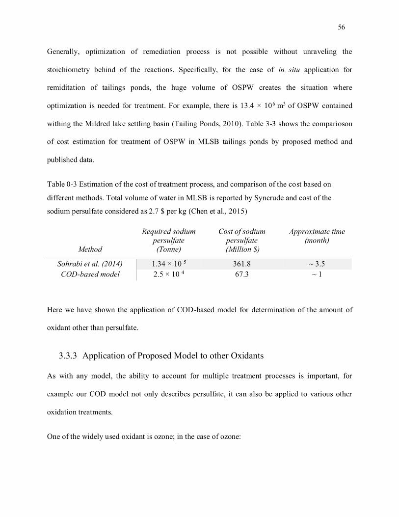
56
Generally, optimization of remediation process is not possible without unraveling the
stoichiometry behind of the reactions. Specifically, for the case of in situ application for
remiditation of tailings ponds, the huge volume of OSPW creates the situation where
optimization is needed for treatment. For example, there is 13.4 × 10⁶ m3 of OSPW contained
withing the Mildred lake settling basin (Tailing Ponds, 2010). Table 3-3 shows the comparioson
of cost estimation for treatment of OSPW in MLSB tailings ponds by proposed method and
published data.
Table 0-3 Estimation of the cost of treatment process, and comparison of the cost based on
different methods. Total volume of water in MLSB is reported by Syncrude and cost of the
sodium persulfate considered as 2.7 $ per kg (Chen et al., 2015)
Method
Required sodium
persulfate
(Tonne)
Cost of sodium
persulfate
(Million $)
Approximate time
(month)
Sohrabi et al. (2014) 1.34 × 10 5 361.8 ~ 3.5
COD-based model 2.5 × 10 4 67.3 ~ 1
Here we have shown the application of COD-based model for determination of the amount of
oxidant other than persulfate.
3.3.3 Application of Proposed Model to other Oxidants
As with any model, the ability to account for multiple treatment processes is important, for
example our COD model not only describes persulfate, it can also be applied to various other
oxidation treatments.
One of the widely used oxidant is ozone; in the case of ozone:
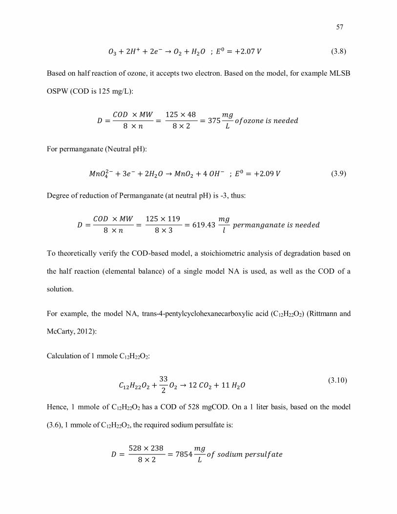
57
𝑂3 + 2𝐻+ + 2𝑒− → 𝑂2 + 𝐻2𝑂 ; 𝐸0 = +2.07 𝑉 (3.8)
Based on half reaction of ozone, it accepts two electron. Based on the model, for example MLSB
OSPW (COD is 125 mg/L):
𝐷 =𝐶𝑂𝐷 × 𝑀𝑊
8 × 𝑛=
125 × 48
8 × 2= 375
𝑚𝑔
𝐿𝑜𝑓𝑜𝑧𝑜𝑛𝑒 𝑖𝑠 𝑛𝑒𝑒𝑑𝑒𝑑
For permanganate (Neutral pH):
𝑀𝑛𝑂42− + 3𝑒− + 2𝐻2𝑂 → 𝑀𝑛𝑂2 + 4 𝑂𝐻− ; 𝐸0 = +2.09 𝑉 (3.9)
Degree of reduction of Permanganate (at neutral pH) is -3, thus:
𝐷 =𝐶𝑂𝐷 × 𝑀𝑊
8 × 𝑛=
125 × 119
8 × 3= 619.43
𝑚𝑔
𝑙 𝑝𝑒𝑟𝑚𝑎𝑛𝑔𝑎𝑛𝑎𝑡𝑒 𝑖𝑠 𝑛𝑒𝑒𝑑𝑒𝑑
To theoretically verify the COD-based model, a stoichiometric analysis of degradation based on
the half reaction (elemental balance) of a single model NA is used, as well as the COD of a
solution.
For example, the model NA, trans-4-pentylcyclohexanecarboxylic acid (C12H22O2) (Rittmann and
McCarty, 2012):
Calculation of 1 mmole C12H22O2:
𝐶12𝐻22𝑂2 +33
2𝑂2 → 12 𝐶𝑂2 + 11 𝐻2𝑂
(3.10)
Hence, 1 mmole of C12H22O2 has a COD of 528 mgCOD. On a 1 liter basis, based on the model
(3.6), 1 mmole of C12H22O2, the required sodium persulfate is:
𝐷 = 528 × 238
8 × 2= 7854
𝑚𝑔
𝐿𝑜𝑓 𝑠𝑜𝑑𝑖𝑢𝑚 𝑝𝑒𝑟𝑠𝑢𝑙𝑓𝑎𝑡𝑒
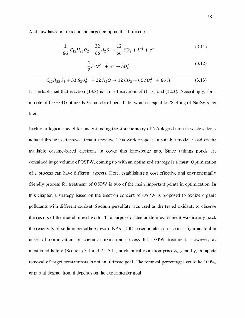
58
And now based on oxidant and target compound half reactions:
1
66 𝐶12𝐻22𝑂2 +
22
66𝐻2𝑂 →
12
66 𝐶𝑂2 + 𝐻+ + 𝑒−
(3.11)
1
2𝑆2𝑂8
2− + 𝑒− → 𝑆𝑂42−
(3.12)
𝐶12𝐻22𝑂2 + 33 𝑆2𝑂82− + 22 𝐻2𝑂 → 12 𝐶𝑂2 + 66 𝑆𝑂4
2− + 66 𝐻+ (3.13)
It is established that reaction (13.3) is sum of reactions of (11.3) and (12.3). Accordingly, for 1
mmole of C12H22O2, it needs 33 mmole of persulfate, which is equal to 7854 mg of Na2S2O8 per
liter.
Lack of a logical model for understanding the stoichiometry of NA degradation in wastewater is
notated through extensive literature review. This work proposes a suitable model based on the
available organic-based electrons to cover this knowledge gap. Since tailings ponds are
contained huge volume of OSPW, coming up with an optimized strategy is a must. Optimization
of a process can have different aspects. Here, establishing a cost effective and envrionemtally
friendly process for treatment of OSPW is two of the main important points in optimization. In
this chapter, a strategy based on the electron concent of OSPW is proposed to oxdize organic
pollutants with different oxidant. Sodium persulfate was used as the tested oxidants to observe
the results of the model in real world. The purpose of degradation experiment was mainly track
the reactivity of sodium persulfate toward NAs. COD-based model can use as a rigorous tool in
onset of optimization of chemical oxidation process for OSPW treatment. However, as
mentioned before (Sections 3.1 and 2.2.5.1), in chemical oxidation process, genrally, complete
removal of target comtaminats is not an ultimate goal. The removal percentages could be 100%,
or partial degradation, it depends on the experimenter goal!

59
The other advantage of this model is its user friendliness. The only experiment that needs to be
done in application of this model is COD test which is a cheap and simple test.
60
3.4 References
Allen EW. 2008a. Process water treatment in Canada’s oil sands industry: I. Target pollutants
and treatment objectives. J. Environ. Eng. Sci. 7:123–138.
Allen EW. 2008b. Process water treatment in Canada’s oil sands industry: II. A review of
emerging technologies. J. Environ. Eng. Sci. 7:499–524.
Brown LD, Pérez-Estrada L, Wang N, El-Din MG, Martin JW, Fedorak PM, Ulrich AC. 2013.
Indigenous microbes survive in situ ozonation improving biodegradation of dissolved
organic matter in aged oil sands process-affected waters. Chemosphere 93:2748–55.
Brown LD, Ulrich AC. 2015. Oil sands naphthenic acids: a review of properties, measurement,
and treatment. Chemosphere 127:276–90.
Chakravarti R, Patrick BN, Barney M, Kusinski G, Devine TM. 2013. Toward the Mechanism of
Corrosion in Crude Oil: A Study Using Vibrational Spectroscopic Techniques at Elevated
Temperatures. Energy & Fuels 27:7905–7914.
Chen K-F, Chang Y-C, Chiou W-T. 2015. Remediation of diesel-contaminated soil using in situ
chemical oxidation (ISCO) and the effects of common oxidants on the indigenous microbial
community: a comparison study. J. Chem. Technol. Biotechnol.:n/a–n/a.
Clemente JS, Fedorak PM. 2005. A review of the occurrence, analyses, toxicity, and
biodegradation of naphthenic acids. Chemosphere 60:585–600.
Clemente JS, Prasad NG., MacKinnon MD, Fedorak PM. 2003. A statistical comparison of
naphthenic acids characterized by gas chromatography–mass spectrometry. Chemosphere
50:1265–1274.
Derungs WA. 1956. Naphthenic Acid Corrosion —An Old Enemy Of the Petroleum Industry ★.
Corrosion 12:41–46.
Drzewicz P, Perez-Estrada L, Alpatova A, Martin JW, Gamal El-Din M. 2012. Impact of
peroxydisulfate in the presence of zero valent iron on the oxidation of cyclohexanoic acid
and naphthenic acids from oil sands process-affected water. Environ. Sci. Technol.
46:8984–91.
Garcia-Garcia E, Ge JQ, Oladiran A, Montgomery B, El-Din MG, Perez-Estrada LC, Stafford
61
JL, Martin JW, Belosevic M. 2011. Ozone treatment ameliorates oil sands process water
toxicity to the mammalian immune system. Water Res. 45:5849–57.
Government of Alberta. 2016. Oil sands quarterly. Open Text Web Site Management.
Grewer DM, Young RF, Whittal RM, Fedorak PM. 2010. Naphthenic acids and other acid-
extractables in water samples from Alberta: what is being measured? Sci. Total Environ.
408:5997–6010.
He Y, Patterson S, Wang N, Hecker M, Martin JW, El-Din MG, Giesy JP, Wiseman SB. 2012.
Toxicity of untreated and ozone-treated oil sands process-affected water (OSPW) to early
life stages of the fathead minnow (Pimephales promelas). Water Res. 46:6359–68.
Headley J V, Peru KM, Barrow MP, Derrick PJ. 2007. Characterization of naphthenic acids from
Athabasca oil sands using electrospray ionization: the significant influence of solvents.
Anal. Chem. 79:6222–9.
Headley J V., McMartin DW. 2004. A review of the occurrence and fate of naphthenic acids in
aquatic environments. J. Environ. Sci. Heal. - Part A Toxic/Hazardous Subst. Environ. Eng.
Holowenko F. 2002. Characterization of naphthenic acids in oil sands wastewaters by gas
chromatography-mass spectrometry. Water Res. 36:2843–2855.
Holowenko FM, MacKinnon MD, Fedorak PM. 2011. Methanogens and sulfate-reducing
bacteria in oil sands fine tailings waste. Can. J. Microbiol.
Huang K-C, Couttenye RA, Hoag GE. 2002. Kinetics of heat-assisted persulfate oxidation of
methyl tert-butyl ether (MTBE). Chemosphere 49:413–420.
Jiveraj MN. 1995. Naphthenic acids extraction and quantitative analy; fourth ed. Syncrude
Canada Ltd.; Research Department; Edmonton; AB.
Kabdasli I, Arslan-Alaton I. 2010. Chemical Oxidation Applications for Industrial Wastewaters.
IWA Publishing 341 p.
Leshuk T, Wong T, Linley S, Peru KM, Headley J V, Gu F. 2016. Solar photocatalytic
degradation of naphthenic acids in oil sands process-affected water. Chemosphere
144:1854–61.
Liang C, Bruell CJ, Marley MC, Sperry KL. 2004. Persulfate oxidation for in situ remediation of
62
TCE. I. Activated by ferrous ion with and without a persulfate-thiosulfate redox couple.
Chemosphere 55:1213–23.
Liu H, Bruton TA, Doyle FM, Sedlak DL. 2014. In situ chemical oxidation of contaminated
groundwater by persulfate: decomposition by Fe(III)- and Mn(IV)-containing oxides and
aquifer materials. Environ. Sci. Technol. 48:10330–6.
van Loosdrecht, M. C., Nielsen, P. H., Lopez-Vazquez, C. M., & Brdjanovic D. 2016.
Experimental Methods in Wastewater Treatment | IWA Publishing. Water Intell. Online.
http://www.iwapublishing.com/books/9781780404745/experimental-methods-wastewater-
treatment.
Mahdavi H, Prasad V, Liu Y, Ulrich AC. 2015. In situ biodegradation of naphthenic acids in oil
sands tailings pond water using indigenous algae-bacteria consortium. Bioresour. Technol.
187:97–105.
Marentette JR, Frank RA, Bartlett AJ, Gillis PL, Hewitt LM, Peru KM, Headley J V, Brunswick
P, Shang D, Parrott JL. 2015. Toxicity of naphthenic acid fraction components extracted
from fresh and aged oil sands process-affected waters, and commercial naphthenic acid
mixtures, to fathead minnow (Pimephales promelas) embryos. Aquat. Toxicol. 164:108–17.
Miskimmin, B., Fedorak P., Lauman R. & VK. 2010. Oil sands water toxicity: A critical review.
Muyzer G, Stams AJM. 2008. The ecology and biotechnology of sulphate-reducing bacteria.
Nat. Rev. Microbiol. 6:441–54.
North SML and A. 2010. Home - Canada’s Oil Sands.
http://www.canadasoilsands.ca/topics/Tailings/Pages/default.aspx.
Oturan MA, Aaron J-J. 2014. Advanced Oxidation Processes in Water/Wastewater Treatment:
Principles and Applications. A Review. Crit. Rev. Environ. Sci. Technol. 44:2577–2641.
Quinlan PJ, Tam KC. 2015. Water treatment technologies for the remediation of naphthenic
acids in oil sands process-affected water. Chem. Eng. J. 279:696–714.
Ramos-Padrón E, Bordenave S, Lin S, Bhaskar IM, Dong X, Sensen CW, Fournier J, Voordouw
G, Gieg LM. 2011. Carbon and sulfur cycling by microbial communities in a gypsum-
treated oil sands tailings pond. Environ. Sci. Technol. 45:439–46.
63
Rice RG. 1996. Applications of ozone for industrial wastewater treatment — A review. Ozone
Sci. Eng. 18:477–515.
Rittmann B, McCarty P. 2012. Environmental biotechnology: principles and applications.
Robinson T, McMullan G, Marchant R, Nigam P. 2001. Remediation of dyes in textile effluent:
a critical review on current treatment technologies with a proposed alternative. Bioresour.
Technol. 77:247–255.
Shu Z, Li C, Belosevic M, Bolton JR, El-Din MG. 2014. Application of a solar UV/chlorine
advanced oxidation process to oil sands process-affected water remediation. Environ. Sci.
Technol. 48:9692–701.
Slavcheva E, Shone B, Turnbull A. 1999. Review of naphthenic acid corrosion in oilrefining. Br.
Corros. J. 34:125–131.
Sohrabi V, Ross MS, Martin JW, Barker JF. 2013. Potential for in situ chemical oxidation of
acid extractable organics in oil sands process affected groundwater. Chemosphere 93:2698–
703.
Sutton NB, Kalisz M, Krupanek J, Marek J, Grotenhuis T, Smidt H, de Weert J, Rijnaarts HHM,
van Gaans P, Keijzer T. 2014. Geochemical and microbiological characteristics during in
situ chemical oxidation and in situ bioremediation at a diesel contaminated site. Environ.
Sci. Technol. 48:2352–60.
Tsitonaki A, PETRI B, CRIMI M, MOSBÆK H, SIEGRIST RL, BJERG PL. 2010. In Situ
Chemical Oxidation of Contaminated Soil and Groundwater Using Persulfate: A Review.
Crit. Rev. Environ. Sci. Technol. 40:55–91.
Wang N, Chelme-Ayala P, Perez-Estrada L, Garcia-Garcia E, Pun J, Martin JW, Belosevic M,
Gamal El-Din M. 2013. Impact of ozonation on naphthenic acids speciation and toxicity of
oil sands process-affected water to Vibrio fischeri and mammalian immune system.
Environ. Sci. Technol. 47:6518–26.
64
CHAPTER 4. OXIDATIVE STRESS INFLUENCE ON
BIODEGRADATION: QUANTITATIVE PHYSIOLOGICAL
STUDY
4.1 Introduction
Implementation of chemical oxidants is common in the treatment of recalcitrant compounds or
partially biodegradable organics in wastewaters (Oturan and Aaron, 2014). As mentioned in
chapter 2 (Section 2.2.5.1) oxidants are chemicals that have a high tendency to accept electrons.
This tendency is demonstrated by their positive and high redox potential.
Peroxydisulfate or persulfate (S2O82-) with a redox potential of 2.1 V is used as a microbial
disinfectant and a fundamental ion in detergents (Ghanizadeh et al., 2015; Oh et al., 2014;
Veschetti et al., 2003; Wordofa, 2014). Recently, persulfate has received much attention as the
newest oxidant in chemical oxidation for environmental engineering purposes specifically for in
situ chemical oxidation (Liu et al., 2014; Siegrist et al., 2011; Sohrabi et al., 2013; Tsitonaki et
al., 2010). There are a number of reasons that make sodium persulfate a good candidate (Liu et
al., 2014; Tsitonaki et al., 2010; Waldemer et al., 2007):
Low price point for the sodium salt
High potential to generate free sulfate radicals under certain conditions
Reactivity to various contaminants
Production of non-toxic by products
High water solubility and high persistency in the environment
65
There are limitations associated with chemical oxidation treatment of contaminated streams.
These include: the high tendency of intermediates to be persistent to chemical oxidation, and the
high cost of the process to reach complete mineralization (Muñoz et al., 2005). As such, interest
in coupling chemical and biological treatment is increasing (Alaton et al., 2004; Esteves et al.,
2016; Guieysse and Norvill, 2014; Marsolek and Rittmann, 2016; Oller et al., 2011). Many
studies have confirmed that chemical oxidant treatment increases biodegradability of recalcitrant
compounds (Anfruns et al., 2013; Brown et al., 2013; Kiliç et al., 2013; Martin et al., 2010;
Merayo et al., 2013; Rizzo, 2011; Sanchis et al., 2013). Cassidy et al. (2009) investigated the
effect of ozone and sodium persulfate on subsequent biodegradation of 2,4-dinitrotoluene.
Removal efficiency of biological degradation of 2,4-dinitrotoluene was 66% by itself. Ozone
pretreatment had efficiency up to 70% oxidation; however, it took 60 days for microorganism to
rebound to uptake remaining pollutant. Sodium persulfate (~12 gL-1) oxidized only 37% of the
2,4-dinitrotoluene and it there were no lag time for 2,4-dinitrotoluene degraders after sodium
persulfate treatment. It means that sodium persulfate did not have any effect on 2,4-
dinitrotoluene degraders (Cassidy et al., 2009). On the other hand, another study about oxidation
of diesel contaminated site with sodium persulfate, potassium permanganate and hydrogen
peroxide shows different results. Based on Chen et al. (2015) findings sodium persulfate has the
most lethal effect on bacterial community (CFU g-1) i.e. complete death at the dosage of 5%
wt/wt (in 30 mL water and 30 g soil) (Chen et al., 2015).
Lee et al. (2000) found that 98% of Fenton-pretreated benz(a)thracene degradaed after 63 days
of incubation; however, for the case of no pre-treatment only 12% of benz(a)thracene degraded
over the same period of time (Lee and Hosomi, 2001). Another study about the persulfate
oxidation for treatment of gasoline contaminated site has interestingly shown absolute decrease
66
in microbial population. Based on 16S rRNA analyses, population returned to their initial value
after 3 months of firs injection of persulfate. However, increase in copy number of alkB gene
imply on relative enrichment of alkane degrading microorganism (Sutton et al., 2014). Pre-
treatment of pendimethaline contaminated soil by Fenton’s reagent is investigated by Miller et al.
(1996). In spite of overall decrease in population of heterotrophic microorganisms, increase in
the concentration of Pseudomonas species was observed (Miller et al., 1996). It can be realized
that chemical pre-treatment provides favorable condition for bioremediation.
Comparison of concentration of methane and sulfate in a mixture of oil sands process affected
water and fluid fine tailings before and after gamma irradiation demonstrated in slight increases
in microbial activity. Aerobic batch biodegradation of commercial NAs (TCI chemical) can have
removal efficiency of 83%. However, pre-ozonated NAs can be degradaed by microorganisms
up to 89% (Boudens et al., 2016).
In general, chemical oxidation as a pre-treatment enhances the bioavailibity of parent
compounds (Kulik et al., 2006; Miller et al., 1996; Sutton et al., 2010) and produces
biodegradable oxidized daughter compounds (Lee and Hosomi, 2001; Oller et al., 2011; Sutton
et al., 2010).
Just as chemical oxidations improve biodegradability of recalcitrant compounds they also induce
an oxidative stress response in microorganisms, which can lead to death. Brown et al. (2013)
studied the survival of the indigenous microbial community during in situ ozonation of aged oil
sands process-affected water. Results showed that a 50 mg/L ozone dose allowed survival of the
indigenous microbial community and that subsequent biodegradation significantly improved in
the treatments (Brown et al., 2013). It is important to note that few studies of this nature exist
67
thus indicating an important knowledge gap when coupling chemical and biological treatment for
in situ treatment scenarios.
The basic physiology of a microorganism can be described by the following equation
(Kristiansen, 1999; Lehninger et al., 2005):
Phenotype = Genotype + Environment (4.1)
Phenotype expresses the observable properties of a cell either quantitative or qualitative. The
phenotype of a cell originating from two sources: the genotype and the environment of the
(micro-) organisms. The genotype addresses the information contained in DNA (The
informational biopolymer DNA (deoxyribonucleic acid) contains all the cell’s hereditary
information) (Bailey, 1986; Lehninger et al., 2005). Cell physiology is categorized as one of the
branches of phenotype of the cell. In cell physiology all the activities that are taken place in cell
to keep the cell alive is studied. Therefore, parameters such as the rate of substrate consumption,
amount of biomass produced per unit of consumed substrate, doubling time, respiration of the
cell, metabolism are quantities that describe physiology of the cell. Some of mentioned
parameters are interface of engineering and biology i.e. substrate consumption rate. Engineering
parameters that imply on the rate (kinetics) and amount (stoichiometry) is applied to explain
some of the quantitative aspects of cell physiology.
As it can be seen in the equation, physiological parameters cover the intrinsic properties of the
cell. Based on equation 4.1, a change in a cell’s phenotype may have a genetic and/or
environmental origin. As such, if environmental conditions are held constant, differences in the
physiology of the cell are due to changes in the genetic properties of the cell. Thus, studying
physiological parameters are very informative for characterizing the behaviour of cells under
68
different conditions (Boender et al., 2009; Heyland et al., 2010; Jørgensen, 2011; Kristiansen,
1999; LaRowe and Amend, 2015; Nielsen et al., 2012; Rittmann and McCarty, 2012; Strous et
al., 1999).
Bacteria have evolved sophisticated molecular mechanisms to activate antioxidant defense genes
during oxidative stress (Harding et al., 2003; Pruchniak et al., 2015; Sies, 1997). Oxidative
damage to proteins are the main physiological signal that activate antioxidant genes (Cabiscol et
al., 2000; Farr and Kogoma, 1991; Storz et al., 1990). The transcriptional activator OxyR and
SoxR are the main redox sensing proteins in bacteria which contain specific regulators for
antioxidant genes (Cabiscol et al., 2000; Chung et al., 2015; Demple, 1991; Farr and Kogoma,
1991; Honn et al., 2016; Liu et al., 2016; Storz et al., 1990). The most common defense
mechanism against oxidative stress is the production of reducing agents by antioxidant genes
such as: NADHP, NADH, β-carotene, α-tocopherol (Cabiscol et al., 2000; Demple, 1991;
Gambino and Cappitelli, 2016; Harding et al., 2003; Pruchniak et al., 2015). However, a defence
mechanism against oxidative stress by means of persulfate salts is still unclear and there are no
biomarkers currently identified (Mörtstedt et al., 2011). Current research suggests that persulfate
directly attacks the proteins around the cell and biomolecules (Cruz et al., 2009; Mensing et al.,
1998; Mörtstedt et al., 2011; Muñoz et al., 2004). Up to date, a significant knowledge gap still
exists in understanding the impact of persulfate on microorganisms.
In this work, for the first time quantitative physiological parameters are tracked for a
Pseudomonas sp. (isolated in our lab group) to elucidate the effect of oxidative stress by the
persulfate ion. We hypothesized that oxidative stress would affect the ability of Pseudomonas sp.
in depletion of Merichem NAs. To characterize the behaviour of Pseudomonas sp. before and
after oxidative stress, the following quantitative physiological parameters will be determined:
69
biomass specific growth rate, biomass specific substrate consumption rate, yield of substrate to
biomass. The biomass specific oxygen consumption rate, and yield of oxygen to biomass as the
representation of the amount of electron acceptor consumed is also discussed (Boender et al.,
2009; Heyland et al., 2010; Jørgensen, 2011; Kristiansen, 1999; LaRowe and Amend, 2015;
Nielsen et al., 2012; Rittmann and McCarty, 2012; Strous et al., 1999).
4.2 Materials and Methods
4.2.1 Substrate, Oxidant and Microorganism Used in Experimental Set-up
Organic substrate. Naphthenic acids (NAs) were selected as the sole source of carbon and
electrons (as discussed above, the selected substrate has to be partially biodegradable)
Commercial NAs were purchased from Merichem Co. (Houston, Texas) and dissolved in 1 N
filtered NaOH as the stock solution of 100 mg/mL for the carbon source.
Chemical oxidant. Sodium persulfate salt 99% was purchased from Sigma-Aldrich. The stock
solution prepared at the concentration of 25 g/L. Assigned amount of sodium persulfate added to
the stress test flasks.
Microorganisms. The Pseudomonas sp. in this study have been isolated from Suncor’s South
Tailings Pond in our lab. Bushnell-Haas minimal medium (Sigma-Aldrich) 3.27 g/L containing
MgSO4 0.2 g, CaCl2 0.02 g, KH2PO4 1 g, K2HPO4 1 g, NH4NO3 1 g, FeCl3 0.05 g per litre of
water and LB Broth Lennox (Fisher Scientific) containing casein peptone 10 g/L, yeast extract 5
g/L, NaCl 5 g/L was used as the bacterial growth media. LB broth used in oxidative stress
experiments and HB broth used in biodegradation experiments.
70
4.2.2 Measurement of Cell Growth and DOC
To track bacterial growth in LB broth optical density at 600 nm was measured over time with
NanoDrop 2000 UV-Vis spectrophotometer (Thermo Scientific). Dry cell weight (DCW) in BH
broth was determined by filtering 25 ml of culture through previously weighed 0.22 µm filters
(Millipore) and then dried at 40oC for 48 hours (Elmén et al., 1997). The DCW measuring
techniques was desired in biodegradation studies for more industrial applicability, and
dimensionally relevant (Elmén et al., 1997; Rittmann and McCarty, 2012) for prediction of
respiratory parameters (oxygen consumption) (Colin Ratledge, 2006; Flickinger, 2009). To track
the depletion of the Merichem NAs, dissolved organic carbon (DOC) measurements were
completed with a TOC Analyser (Shimadzu TOC-L CPH, Japan). For DOC analysis, potassium
hydrogen phathalate ≥ 99.95% (Sigma-Aldrich) used to make standard solution for calibration.
And inorganic carbon was removed by adding 2.3% (v/v) 2 N HCl and airflow was adjusted to
50 ml/min for 3 min and organic carbon combusted at 680oC.
4.2.3 Oxidative Stress Test
Oxidative stress tests were carried out in batch cultivation using 1 L shaking flasks with 500 mL
of LB broth. The same amount of the Pseudomonas sp. isolate (at OD of 1.2) was added into
each flask. Four different concentrations of Na2S2O8 were added to each flask: 0, 250, 500, 1000
and 2000 mg/L. Tested dosages were determined based on the obtained results in chapter 3. The
dosages of persulfate selected based on the estimated amount of persulfate needed for NAs
degradation (See section 3.3.2). Each treatment was conducted in triplicate at room temperature
(21±3o C) and flasks were shake at 200 rpm. Once stationary phase was achieved in each
treatment, a 500 µL aliquot was prepped and transferred to freshly set-up flasks to determine the
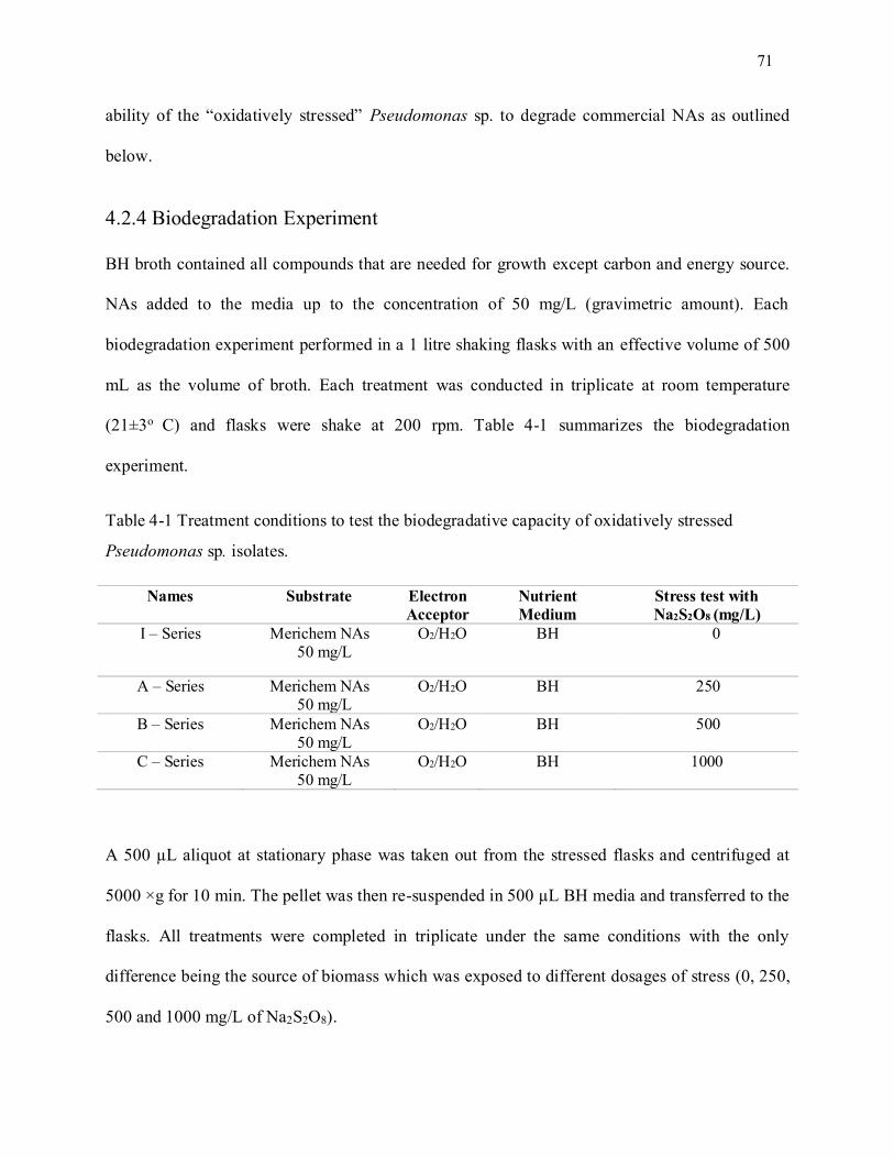
71
ability of the “oxidatively stressed” Pseudomonas sp. to degrade commercial NAs as outlined
below.
4.2.4 Biodegradation Experiment
BH broth contained all compounds that are needed for growth except carbon and energy source.
NAs added to the media up to the concentration of 50 mg/L (gravimetric amount). Each
biodegradation experiment performed in a 1 litre shaking flasks with an effective volume of 500
mL as the volume of broth. Each treatment was conducted in triplicate at room temperature
(21±3o C) and flasks were shake at 200 rpm. Table 4-1 summarizes the biodegradation
experiment.
Table 4-1 Treatment conditions to test the biodegradative capacity of oxidatively stressed
Pseudomonas sp. isolates.
Names Substrate Electron
Acceptor
Nutrient
Medium
Stress test with
Na2S2O8 (mg/L)
I – Series Merichem NAs 50 mg/L
O2/H2O BH 0
A – Series Merichem NAs 50 mg/L
O2/H2O BH 250
B – Series Merichem NAs 50 mg/L
O2/H2O BH 500
C – Series Merichem NAs 50 mg/L
O2/H2O BH 1000
A 500 µL aliquot at stationary phase was taken out from the stressed flasks and centrifuged at
5000 ×g for 10 min. The pellet was then re-suspended in 500 µL BH media and transferred to the
flasks. All treatments were completed in triplicate under the same conditions with the only
difference being the source of biomass which was exposed to different dosages of stress (0, 250,
500 and 1000 mg/L of Na2S2O8).
72
4.3 Results and Discussion
4.3.1 Biodegradative Capacity of Pseudomonas sp.
Pseudomonas species have shown a strong ability to uptake a wide range of organic substrates as
their sole carbon and energy source (Hack et al., 2015; Huang et al., 2016; Patel et al., 2012;
Reardon et al., 2000; Silver et al., 1990; Zhang et al., 2016). Pseudomonas species have
nonspecificity of induced enzymes and convergence of catabolic pathways, allowing them to
utilize mixed substrates without any surplus genetic coding for enzyme production (Hutchinson
and Robinson, 1988; Silver et al., 1990). Based on this capacity, Pseudomonas species, can be
considered a potential candidate for degradation of NAs (Blakley and Papish, 1982; Demeter et
al., 2015; Paslawski et al., 2009; Del Rio et al., 2006; Whitby, 2010).
4.3.2 Impact of Persulfate Oxidative Stress on Pseudomonas sp
To determine the impact of persulfate oxidative stress on the Pseudomonas sp. the growth curve
of the isolate was monitored as it was exposed to 0- 2000 mg/L of persulfate in a LB broth
media. As shown in figure 4.1 the maximum biomass concentration decreases from 1.260 AU
(ideal growth) to 0 (2000 mg/L of sodium persulfate) with increasing the persulfate
concentration.
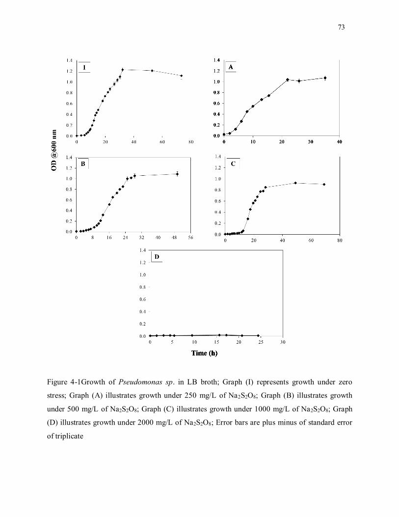
73
Figure 4-1Growth of Pseudomonas sp. in LB broth; Graph (I) represents growth under zero
stress; Graph (A) illustrates growth under 250 mg/L of Na2S2O8; Graph (B) illustrates growth
under 500 mg/L of Na2S2O8; Graph (C) illustrates growth under 1000 mg/L of Na2S2O8; Graph
(D) illustrates growth under 2000 mg/L of Na2S2O8; Error bars are plus minus of standard error
of triplicate
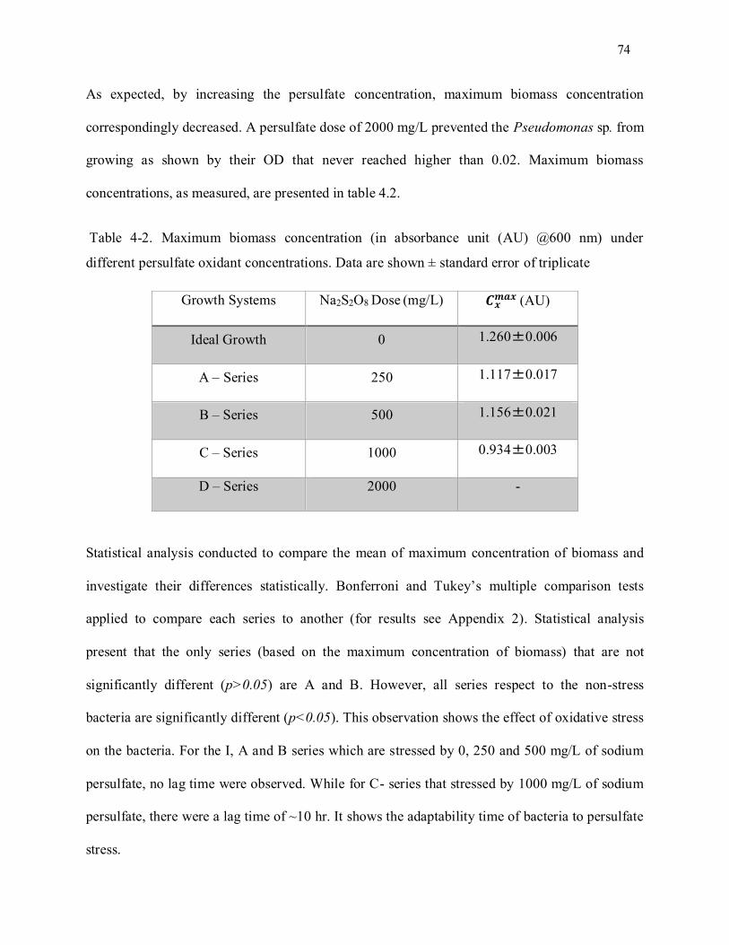
74
As expected, by increasing the persulfate concentration, maximum biomass concentration
correspondingly decreased. A persulfate dose of 2000 mg/L prevented the Pseudomonas sp. from
growing as shown by their OD that never reached higher than 0.02. Maximum biomass
concentrations, as measured, are presented in table 4.2.
Table 4-2. Maximum biomass concentration (in absorbance unit (AU) @600 nm) under
different persulfate oxidant concentrations. Data are shown ± standard error of triplicate
Growth Systems Na2S2O8 Dose (mg/L) 𝑪𝒙𝒎𝒂𝒙 (AU)
Ideal Growth 0 1.260±0.006
A – Series 250 1.117±0.017
B – Series 500 1.156±0.021
C – Series 1000 0.934±0.003
D – Series 2000 -
Statistical analysis conducted to compare the mean of maximum concentration of biomass and
investigate their differences statistically. Bonferroni and Tukey’s multiple comparison tests
applied to compare each series to another (for results see Appendix 2). Statistical analysis
present that the only series (based on the maximum concentration of biomass) that are not
significantly different (p>0.05) are A and B. However, all series respect to the non-stress
bacteria are significantly different (p<0.05). This observation shows the effect of oxidative stress
on the bacteria. For the I, A and B series which are stressed by 0, 250 and 500 mg/L of sodium
persulfate, no lag time were observed. While for C- series that stressed by 1000 mg/L of sodium
persulfate, there were a lag time of ~10 hr. It shows the adaptability time of bacteria to persulfate
stress.
75
Pseudomonas sp. are aerobic bacteria that are uses oxygen as the electron acceptor. To have an
understanding of oxygen mass transfer in flasks as the bioreactor, mass transfer analysis
perforemed, as follows.
4.3.3 Mass Transfer Analysis
One of the main factors that might affect the aerobic bioprocesses is limitation oxygen transfer.
To ensure that oxygen was not a limiting factor in our system and keep the degree of the freedom
of the system to one (the only degree of freedom in our system was concentration of substrate
which was Merichem NAs). Transfer of oxygen takes place through two phases in our
experiments. First, the transfer of oxygen from gas phase (from the bottleneck of the flask to the
interface of liquid and gas phases). Second, transfer of oxygen in the liquid phase.
4.3.3.1 Oxygen Mass Transfer Coefficient in Gas Phase
To calculate the oxygen mass transfer coefficient in the gas phase (kGa) we need to know the
turbulence factor (TG) in the gas phase. There is an empirical formula for calculating the
turbulence factor as a function of flask to liquid volume ratio and rate of shaking (Nikakhtari and
Hill, 2006):
For a flask without a closure, α is equal to 1.80. TG represents the gas phase turbulence factor. By
knowing the TG; one can calculate the oxygen mass transfer coefficient in the gas phase as
(Nikakhtari and Hill, 2006):
𝑇𝐺 =𝑉
𝐿× 𝑁𝛼
(4.1A)
𝑘𝐺𝑎= 0.176 ∙ exp (0.0002 × 𝑇𝐺) (4.2)
76
In the above equations, kGa is the mass transfer coefficient in the liquid phase; V is the volume of
the flask; L is the volume of liquid; TG is the gas phase turbulence factor and N is the shaking
rate (Nikakhtari and Hill, 2005). However, this equation is valid for TG =11000 ± 400; for TG
more than 11000 an average value of 86.8 ± 15.7 h -1 is considered. Practically, for this range of
kGa (~86.8 ± 15.7 h -1) resistance against mass transfer of oxygen through the neck of the shake
flask to the headspace is negligible (Gupta and Rao, 2003; Henzler and Schedel, 1991;
Nikakhtari and Hill, 2006; Van Suijdam et al., 1978; Veglio et al., 1998). It can be seen that in
table 4-3 the kGa for our experiments is high enough, therefore, the resistance against mass
transfer of oxygen in gas phase is negligible. Table 4-3 shows the TG value for this work.
Table 4-3. Oxygen mass transfer coefficient in the gas phase is calculated. V shows the volume
of the flask, L represents the liquid volume of the flask; N is the mixing rate; α is constant and
TG is turbulence factor which is calculated based on Eq. 4.27.
V (L) L (L) N (rpm) α TG kGa (h -1)
Beginning of the
experiment
1 0.5 200 1.80 27726 86.8 ± 15.7
End of the experiment 1 0.25 200 1.80 55452 86.8 ± 15.7
4.3.3.2 Oxygen Mass Trasnfer Coefficient in Liquid Phase
Oxygen mass transfer coefficient in the liquid phase can be calculated based on the following
equations (Nikakhtari and Hill, 2005):
𝑘𝐿𝑎= 0.0182 × (𝐴 × 𝑇𝐿)
(4.3)
𝐴 = 142 × (𝑉 − 𝐿)2/3 (4.4)
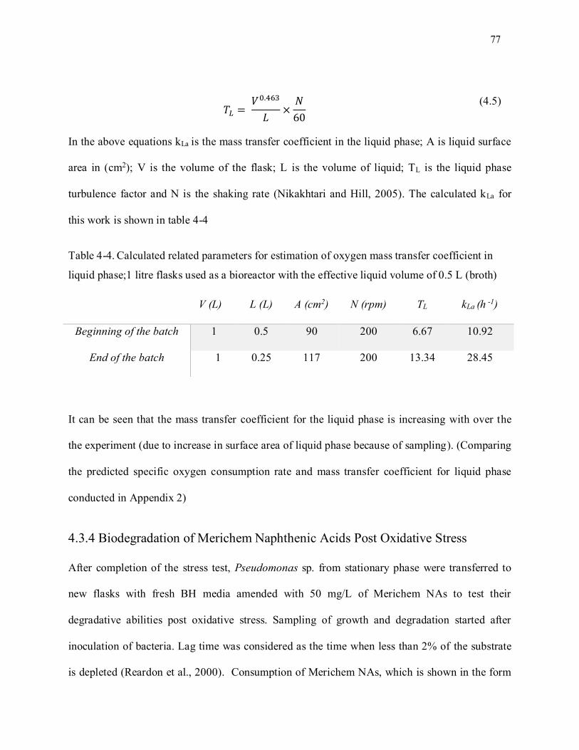
77
In the above equations kLa is the mass transfer coefficient in the liquid phase; A is liquid surface
area in (cm2); V is the volume of the flask; L is the volume of liquid; TL is the liquid phase
turbulence factor and N is the shaking rate (Nikakhtari and Hill, 2005). The calculated kLa for
this work is shown in table 4-4
Table 4-4. Calculated related parameters for estimation of oxygen mass transfer coefficient in
liquid phase;1 litre flasks used as a bioreactor with the effective liquid volume of 0.5 L (broth)
V (L) L (L) A (cm2) N (rpm) TL kLa (h -1)
Beginning of the batch 1 0.5 90 200 6.67 10.92
End of the batch 1 0.25 117 200 13.34 28.45
It can be seen that the mass transfer coefficient for the liquid phase is increasing with over the
the experiment (due to increase in surface area of liquid phase because of sampling). (Comparing
the predicted specific oxygen consumption rate and mass transfer coefficient for liquid phase
conducted in Appendix 2)
4.3.4 Biodegradation of Merichem Naphthenic Acids Post Oxidative Stress
After completion of the stress test, Pseudomonas sp. from stationary phase were transferred to
new flasks with fresh BH media amended with 50 mg/L of Merichem NAs to test their
degradative abilities post oxidative stress. Sampling of growth and degradation started after
inoculation of bacteria. Lag time was considered as the time when less than 2% of the substrate
is depleted (Reardon et al., 2000). Consumption of Merichem NAs, which is shown in the form
𝑇𝐿 = 𝑉0.463
𝐿×
𝑁
60
(4.5)
78
of dissolved organic carbon shows the capacity for the Pseudomonas sp. to grow on Merichem
NAs as the sole source of carbon and energy (as shown in Figure 4-2). Kinetic and
stoichiometric (physiological) analysis was completed to compare the performance of bacteria
under different cultivation conditions. It is interesting to mention that the “bottle effect” or
surface to volume ratio has no effect on biodegradation and concentration of biomass in batch
growth conditions (Hammes et al., 2010).
Calculation of stoichiometric and kinetic parameters can be quite challenging for partially
biodegradable substrates. As can be seen Merichem NAs are also partially biodegradable by
Pseudomonas sp. As mentioned in chapter 2, physiological parameters from batch data are not as
reliable as chemostat cultivation (Kovarova-Kovar and Egli, 1998). For instance, there is no
information about Ks (substrate affinity) of biodegradation of commercial NAs or AEOs to a
given microorganism. Lack of such data affects parameter estimation. Ellis et al. (1996)
conducted a sensitivity analysis to estimate the influence of each parameter of the Monod
equation in parameter estimation processes and suggested that when 𝐶0
𝐾𝑠 < 0.1, unique estimation
of qmax and Ks is not possible (Ellis et al., 1996; Knightes and Peters, 2000).
Linearization of the Monod equation and then using linear regression analysis to estimate the
parameter is another method that can be used (Cornish-Bowden, 2013; Krull and Peterat, 2016).
This method is widely used in the estimation of parameters in biodegradation studies,
fermentation and enzymes kinetic studies, however, it is infamous for being prone to error
(Cornish-Bowden, 2013; Leatherbarrow, 1990). Because the Monod model (since it is a linear
regression) assumes the errors are normally distributed and since linearization highly alters the
79
errors, results cannot be reliable (Cornish-Bowden, 2013; Knightes and Peters, 2000;
Leatherbarrow, 1990).
To overcome all the difficulties associated with parameter estimation we can use a direct method
to calculate certain kinetic and stoichiometric parameters. Direct method analysis is completed
based on a mass balance and rate calculation (Smolke, 2009; Stephanopoulos et al., 1998;
Villadsen et al., 2011). In this approach to be scientifically relevant, we consider the log-phase
when analysing the data. We take into account data which are after the lag time. As it mentioned
above, the lag time is a time when less than 2% of the substrate is depleted (Reardon et al.,
2000). Each batch ends at the first time point when it reaches the highest concentration of
biomass. And as it can be seen in figure 4-2, the highest concentration of biomass is the time
when the batch reaches the lowest concentration of substrate.
4.3.5 Mathematical Modelling Based on Mass Balance
The mass balance in batch cultivation can be described as follows (Kristiansen, 1999; Rittmann
and McCarty, 2012; Smolke, 2009):
Accumulation of compound i = Rate i (4.6)
𝑅𝑎𝑡𝑒 𝑖 = 𝑑(𝑉. 𝐶𝑖)
𝑑𝑡=
𝑑𝑀𝑖
𝑑𝑡
(4.6A)
In the above equation, V represent the volume, Ci shows the concentration of compound I; t is
time and Mi illustrates the total mass of the compound i in the system. By definition, for
consumed compounds the rate is negative and for produced compounds is positive. One very
important point about the calculation of physiological parameters is considering the volume
changes through batch time. So by considering the changes in volume (Smolke, 2009):
80
Throughout the experiment the changes in volume due to evaporation were negligible. So instead
of using total mass we can continue using concentration in our rate calculations.
q-rates which are biomass specific rates are defined as follows (See section 2.4.2) (Smolke,
2009; Stephanopoulos et al., 1998):
In Eq. (4.8) qi represents the biomass specific rate of compound i. For instance, rs is the substrate
consumption rate. Based on Eq. (2.8) the substrate consumption rate has a direct relation to
concentration of biomass. It means that rs will increase by increasing in concentration of
biomass. Therefore, rs is a dependent parameter which means one cannot use this parameter to
describe the performance of the biomass in the system. For instance, rs,1 = 30 mg L-1 h-1 and rs,2
=20 mg L-1 h-1 for two different independent system. It is obvious that bioreactor one has higher
rate i.e. in removal of substrate. However, we do not know about the performance of biomass in
these two systems and we cannot analyse the ability of microorganisms in consumption of
substrate unless we know the concentration of biomass. The concentration of biomass is as
follows: Cx,1=10 mg L-1 and Cx,2=4 mg L-1. Based on the Eq. (4.8); qs,1= 3 mg Cs mg Cx-1 h-1
qs,2= 5 mg Cs mg Cx-1 h-1 ; therefore, it can be seen that substrate consumption rate is faster per
unit of biomass in bioreactor 2. It shows the microorganisms are better for our goal (i.e.
remediation purposes). Accordingly, it is very important to compare appropriate parameters in
evaluation of the performance of bioprocesses. By definition, qx is equal to µ which is a specific
growth rate. Now we can write up the equation for calculation of biomass growth rate
𝑅𝑎𝑡𝑒 𝑖 = 𝑑(𝑉. 𝐶𝑖)
𝑑𝑡= 𝐶𝑖
𝑑𝑉
𝑑𝑡+ 𝑉
𝑑𝐶𝑖
𝑑𝑡
(4.7)
𝑞𝑖 = 𝑟𝑖
𝐶𝑥
(4.8)
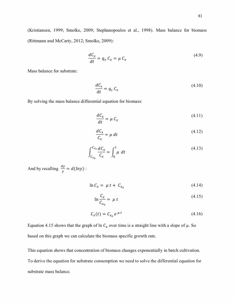
81
(Kristiansen, 1999; Smolke, 2009; Stephanopoulos et al., 1998). Mass balance for biomass
(Rittmann and McCarty, 2012; Smolke, 2009):
Mass balance for substrate:
By solving the mass balance differential equation for biomass:
And by recalling 𝑑𝑦
𝑦= 𝑑(𝑙𝑛𝑦) :
Equation 4.15 shows that the graph of ln 𝐶𝑥 over time is a straight line with a slope of µ. So
based on this graph we can calculate the biomass specific growth rate.
This equation shows that concentration of biomass changes exponentially in batch cultivation.
To derive the equation for substrate consumption we need to solve the differential equation for
substrate mass balance.
𝑑𝐶𝑥
𝑑𝑡= 𝑞𝑥 𝐶𝑥 = 𝜇 𝐶𝑥
(4.9)
𝑑𝐶𝑠
𝑑𝑡= 𝑞𝑠 𝐶𝑥
(4.10)
𝑑𝐶𝑥
𝑑𝑡= 𝜇 𝐶𝑥
(4.11)
𝑑𝐶𝑥
𝐶𝑥
= 𝜇 𝑑𝑡 (4.12)
∫𝑑𝐶𝑥
𝐶𝑥
𝐶𝑥𝑡
𝐶𝑥0
= ∫ 𝜇𝑡
0
𝑑𝑡 (4.13)
ln 𝐶𝑥 = 𝜇 𝑡 + 𝐶𝑥0 (4.14)
ln𝐶𝑥
𝐶𝑥0
= 𝜇 𝑡 (4.15)
𝐶𝑥(𝑡) = 𝐶𝑥0 𝑒 𝜇 𝑡 (4.16)
82
By recalling 𝑑𝑒𝑢(𝑥)
𝑑𝑥= 𝑒𝑢(𝑥) 𝑑𝑢(𝑥)
𝑑𝑥 :
By integrating the above equation:
In equation 4.22 the only unknown parameter is 𝑞𝑠. We can determine µ from equation 4.15,
therefore to calculate 𝑞𝑠:
Term of 𝐶𝑥0 (𝑒 𝜇 ∙ 𝑡) is equal to 𝐶𝑥(𝑡) based on equation 4.16. Thus:
𝑑𝐶𝑠
𝑑𝑡= 𝑞𝑠 𝐶𝑥
(4.17)
𝑑𝐶𝑠
𝑑𝑡= 𝑞𝑠 𝐶𝑥0 𝑒
𝜇 𝑡 (4.18)
𝑑𝐶𝑠 = (𝑞𝑠 ∙ 𝐶𝑥0 )[(𝑒 𝜇 ∙ 𝑡)𝑑𝑡]
(4.19)
𝑑𝐶𝑠 = ((𝑞𝑠 ∙ 𝐶𝑥0 )
𝜇) [𝑑(𝑒 𝜇 ∙ 𝑡)]
(4.20)
∫ 𝑑𝐶𝑠
𝐶𝑠𝑡
𝐶𝑠0
= ∫ ((𝑞𝑠 𝐶𝑥0 )
𝜇) [𝑑(𝑒 𝜇 ∙ 𝑡)]
𝑡
0
(4.21)
𝐶𝑠(𝑡) − 𝐶𝑠0= (
(𝑞𝑠 𝐶𝑥0 )
𝜇) ((𝑒 𝜇 ∙ 𝑡) − 1)
(4.22)
𝐶𝑠(𝑡) − 𝐶𝑠0= (
𝑞𝑠
𝜇) (𝐶𝑥0
(𝑒 𝜇 𝑡) − 𝐶𝑥0 ) (4.23)
𝐶𝑠(𝑡) − 𝐶𝑠0= (
𝑞𝑠
𝜇) (𝐶𝑥(𝑡) − 𝐶𝑥0 )
(4.24)
𝐶𝑥(𝑡) − 𝐶𝑥0
𝐶𝑠(𝑡) − 𝐶𝑠0
=𝜇
𝑞𝑠
(4.25)
83
This reltionship demonstrates that the plot of 𝐶𝑠(𝑡) − 𝐶𝑠0 and 𝐶𝑥(𝑡) − 𝐶𝑥0
is a straight line. The
slope of this straight line is equal to 𝜇
𝑞𝑠 . This slope represents the ratio of these two rates which
corresponds to the yield. One important yield, as a stoichiometric parameter, is the yield of
substrate to the biomass. This yield demonstrates the biomass production per unit of consumed
substrate. We can calculate this yield by dividing the rate of biomass growth and substrate
consumption rate (Kovarova-Kovar and Egli, 1998; Rittmann and McCarty, 2012; Smolke, 2009;
Stephanopoulos et al., 1998).
This yield can be calculated from the slope of the plot of (Cx – Cx0) and (Cs – Cs0). In Fig 4.3 Ln
(Cx/Cx0) is plotted over time to calculate the specific growth rate. In Fig 4.4 (Cx – Cx0) is plotted
over (Cs – Cs0) to calculate the yield of the substrate to biomass.
𝑌𝑠𝑥 =𝑅𝑎𝑡𝑒 𝐶𝑥
𝑅𝑎𝑡𝑒 𝐶𝑠=
𝜇 𝐶𝑥
𝑞𝑠 𝐶𝑥=
𝜇
𝑞𝑠
(4.26)
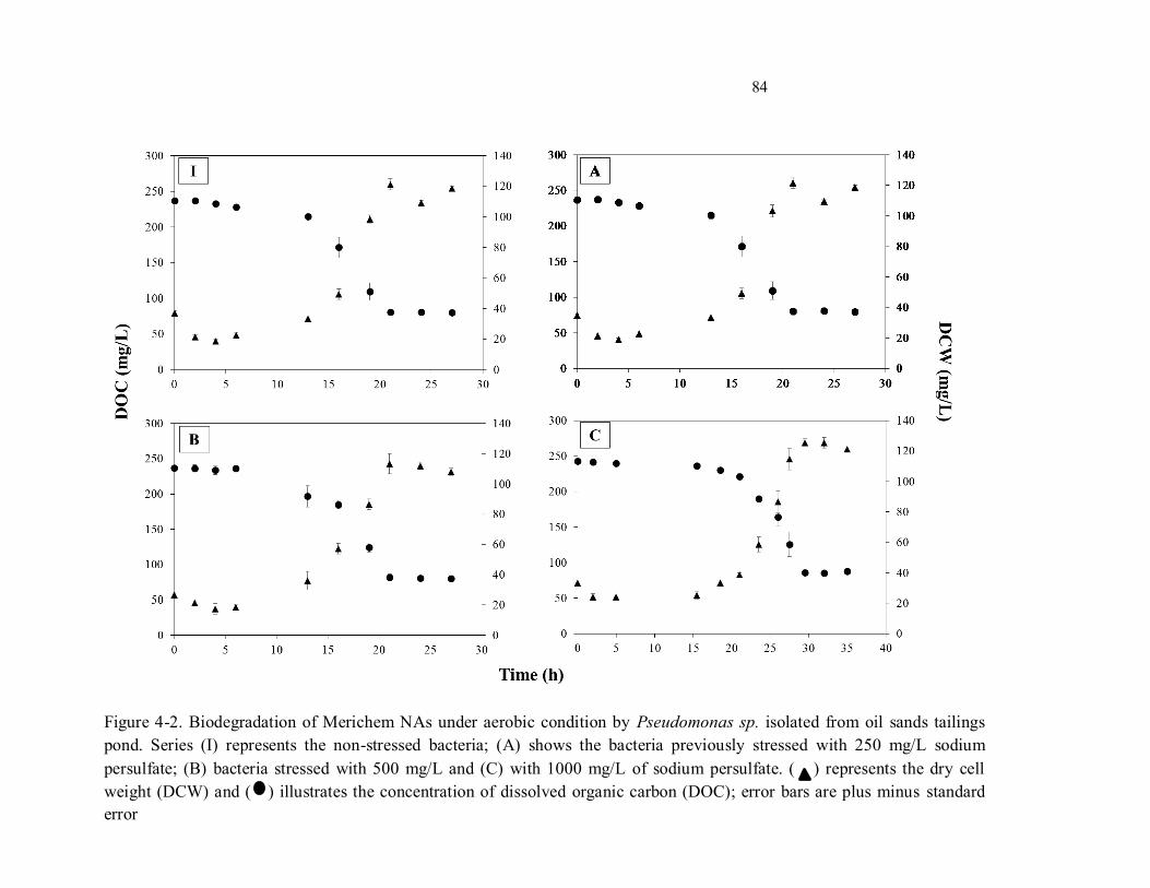
84
Figure 4-2. Biodegradation of Merichem NAs under aerobic condition by Pseudomonas sp. isolated from oil sands tailings
pond. Series (I) represents the non-stressed bacteria; (A) shows the bacteria previously stressed with 250 mg/L sodium
persulfate; (B) bacteria stressed with 500 mg/L and (C) with 1000 mg/L of sodium persulfate. ( ) represents the dry cell
weight (DCW) and ( ) illustrates the concentration of dissolved organic carbon (DOC); error bars are plus minus standard
error
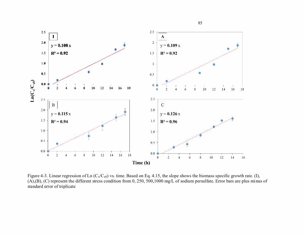
85
Figure 4-3. Linear regression of Ln (Cx/Cx0) vs. time. Based on Eq. 4.15, the slope shows the biomass specific growth rate. (I),
(A),(B), (C) represent the different stress condition from 0, 250, 500,1000 mg/L of sodium persulfate. Error bars are plus minus of
standard error of triplicate
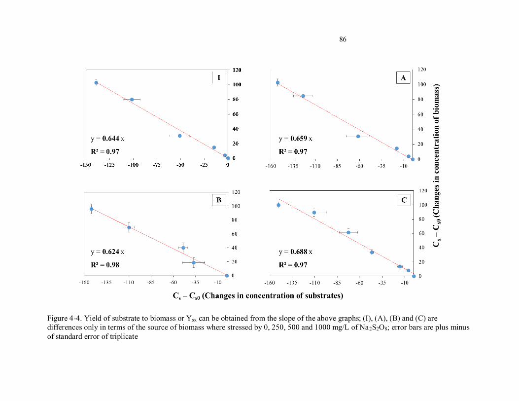
86
Figure 4-4. Yield of substrate to biomass or Ysx can be obtained from the slope of the above graphs; (I), (A), (B) and (C) are
differences only in terms of the source of biomass where stressed by 0, 250, 500 and 1000 mg/L of Na2S2O8; error bars are plus minus
of standard error of triplicate
87
4.3.5.1 Biomass specific growth rate
Results that are derived from Eq (4.15) are summerised in table 4-5. Biomass doubling time of
the biomass is also shown to have better representation of growth rate.
Table 4-5. Biomass specific growth rate and doubling time of biomass
µ biomass specific growth rate (h-1
) tD doubling time (h)
Average 95% Confidence Interval Average 95% Confidence Interval
I 0.108 0.091 - 0.124 6.42 7.62 - 5.59
A 0.109 0.092 - 0.126 6.36 7.53 - 5.50
B 0.115 0.099 - 0.131 6.03 7.00 - 5.29
C 0.126 0.114 - 0.138 5.50 6.08 - 5.02
Biomass specific growth rate represents the rate of biosynthesis of new cells. This rate is a
function of different parametres i.e. temperature, amount of nutrient, concentration of substrate.
This rate is representation of anabolism which is an intrinsic property of a cell. The changes in
the rate of anabolism (biomass specific growth rate) in the batch process can have (in general)
two degree of freedom, one for the environment and one for its intrinsic properties. Therefore, in
the same environmental condition a change in the rate of anabolism has only one degree of
freedom. This degree of freedom originates from the gene expression of the microorganisms, as
genes control all of the cell’s activity.
Biomass specific growth rates for each set of experiment determined as an independent
parameter for comparison of the performance of bacteria. This parameter as introduced in
chapter 2 (section 2.4.2), is a kinetic parameter. Results are showing no significant (p>>0.05)
changes in kinetic of biomass specific growth rate. It means that changes in genetic expression of
Pseudomonas sp. due to oxidative stress did not effect on the ability of the bacteria to grow on
Merichem NAs. This observation enhances the chance of coupling chemical and biological
88
oxidation. However, there is a lag time in biodegrdation, after rebounding, the bacteria can grow
as the same as non-stressed bacteria. For treatment purposes, the growth rate is one of the (many)
factors are implementation of a process. Therefore, other related parameters are discussed, as
follows.
4.3.5.2 Yield of Substrate to Biomass (Ysx)
In analyses of the amount of biomass that is produced per unit of consumed substrate based on
Fig 4-4, following results are obtained. Generally, understanding of yield of substrate to biomass
is among the most important parameters in design and application of a biological process
(Rittmann and McCarty, 2012). In design of a bioprocess, the amount of produced biomass is
very important. Lack of this information would result in i.e. high production rate of CO2 (mainly
because of catabolism), high rate of biomass production which increases the cost of sludge
handling.
Table 4-6. Yield of substrate to biomass for non-stressed and previously stressed bacteria
Ysx (mg DCW mgDOC -1)
Average 95% Confidence Interval
I 0.644 0.586 - 0.703
A 0.659 0.600 - 0.717
B 0.624 0.575 - 0.673
C 0.688 0.628 - 0.748
Here, by comparing the yields from each set of experiments, no changes were observed. This
observation expresses that oxiadtively stressed bacteria use the same stoichiometric amount of
substrate to produce biomass. Yield of substrate to biomass is the result of coupling of
catabolism and anabolism. Surprisingly, the yield of substrate to biomass did not change
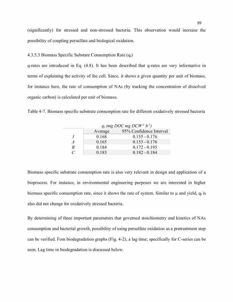
89
(significantly) for stressed and non-stressed bacteria. This observation would increase the
possibility of coupling persulfate and biological oxidation.
4.3.5.3 Biomass Specific Substare Consumption Rate (qs)
q-rates are introduced in Eq. (4.8). It has been described that q-rates are very informative in
terms of explaining the activity of the cell. Since, it shows a given quantity per unit of biomass,
for instance here, the rate of consumption of NAs (by tracking the concentration of dissolved
organic carbon) is calculated per unit of biomass.
Table 4-7. Biomass specific substrate consumption rate for different oxidatively stressed bacteria
qs (mg DOC mg DCW-1 h-1)
Average 95% Confidence Interval
I 0.168 0.155 - 0.176
A 0.165 0.153 - 0.176
B 0.184 0.172 - 0.195
C 0.183 0.182 - 0.184
Biomass specific substrate consumption rate is also very relevant in design and application of a
bioprocess. For instance, in environmental engineering purposes we are interested in higher
biomass specific consumption rate, since it shows the rate of system. Similar to µ and yield, qs is
also did not change for oxidatively stressed bacteria.
By determining of three important parameters that governed stoichiometry and kinetics of NAs
consumption and bacterial growth, possibility of using persulfate oxidation as a pretreatment step
can be verified. Fom biodegradation graphs (Fig. 4-2), a lag time; specifically for C-series can be
seen. Lag time in biodegradation is discussed below.
90
4.3.6 Lag Time of Biodegradation
The 2% biodegradation removal time considered as the lag time of system (Reardon et al., 2000).
Lag time for I, A and B series calculated as 4 hours. 0, 250 and 500 mg/L of sodium persulfate
stressed bacteria has the same amount of lag time. However, for the series of C the calculated lag
time was 15.5 hours. The bacetria that stressed with highest concentration of sodium persulfate
had the longest lag time. The lag time generally defines as the time of adaptability of
microorganisms to current condition. After adaptation of bacteria to the current condition, the
process parameters, as shown above, were not significantly different.
4.4 Conclusions
In this chapter, quantitave physiological study applied to elucidate the effect of oxidative stress
on the ability of microorganisms in using Merichem NAs as the sole source of carbon and
energy. The parameters that are used in quantitative physiological study were chosen base on
their applicability in future desin of the process. The process parametres that are obtained from
non-stressed microorganism are considered as the control, and therefore, parametres from
stressed bacteria compared to the non-stressed ones. Results are showing no significant change in
process parameters of biodegradation, except lag time. For instance, for the bacteria that
previously stressed with 1000 mg/L of sodium persulfate, the lag time was more than 3 times
higher respect to other series.
Other investigation on the effect of persulfate on microorganism have similar findings. However,
changes in kinetic and stoichiometric parameters due to persulfate stress have not been reported.
Palmroth et al. (2006) used counting techniques to demonstrate the effect of persulfate on
indigenous population of soil. Based on their founding, after 2 days of exposure of soil to the
persulfate with the dosage of 10 g/kg soil, the concentration of microorganism decreased from
91
107.5 to 107.4 CFU/g soil (Palmroth et al. 2006). Tsitonaki et al. (2007) tested the range of 0.02 to
2 g S2O8 2-/kg soil on soil indigenous microorganisms. After 2 days as the exposure time,
significant change in the concentration of indigenous microorganisms did not observe. While, the
concentration of spiked Pseudomonas putida decreased from 2.96 × 10⁶ live cells/g soil to 3.4 ×
105 cells/g soil for heat activated persulfate (0.8 g/L) (Tsitonaki et al., 2008). Cassidy et al.
(2009) compared the effect of three oxidants as follows ozone, Fenton and sodium persulfate.
Results have shown that the least amount of effect occurred by sodium persulfate. Rebounding
time (lag time of biodegradation) were as follows: 60 days for ozone, 20 days for Fenton treated
matrix and 2 days for persulfate treated soil (Cassidy et al., 2009).
However, there is a lack of kinetic and stoichiometric parameters of microorganisms before and
after oxidative stress, other findings are imply on the fact that persulfate does not significantly
affect miroorganisms.
Findings of this work can be used in design of a coupled process of chemical and biological
oxidation with persulfate as the oxidant. Tested dosages in chapter 3 of this work shows the
reactivity of persulfate toward main pollutant in OSPW which is NAs. Stressed microorganisms
with the ranages of persulfate that are reactive to NAs, do not significantly affect
biodegradability of Pseudomonas sp. Therefore, combination of persulfate oxidation and
biological oxidation is feasible. However, further experiments is required to apply the process at
industrial scales.
92
4.5 References
Alaton IA, Dogruel S, Baykal E, Gerone G. 2004. Combined chemical and biological oxidation
of penicillin formulation effluent. J. Environ. Manage. 73:155–63.
Anfruns A, Gabarró J, Gonzalez-Olmos R, Puig S, Balaguer MD, Colprim J. 2013. Coupling
anammox and advanced oxidation-based technologies for mature landfill leachate treatment.
J. Hazard. Mater. 258-259:27–34.
Bailey JE. 1986. Biochemical Engineering Fundamentals. McGraw-Hill 984 p.
Blakley ER, Papish B. 1982. The metabolism of cyclohexanecarboxylic acid and 3-
cyclohexenecarboxylic acid by Pseudomonas putida. Can. J. Microbiol. 28:1324–9.
Boender LGM, de Hulster EAF, van Maris AJA, Daran-Lapujade PAS, Pronk JT. 2009.
Quantitative physiology of Saccharomyces cerevisiae at near-zero specific growth rates.
Appl. Environ. Microbiol. 75:5607–14.
Boudens R, Reid T, VanMensel D, Prakasan M R S, Ciborowski JJH, Weisener CG. 2016. Bio-
physicochemical effects of gamma irradiation treatment for naphthenic acids in oil sands
fluid fine tailings. Sci. Total Environ. 539:114–24.
Brown LD, Pérez-Estrada L, Wang N, El-Din MG, Martin JW, Fedorak PM, Ulrich AC. 2013.
Indigenous microbes survive in situ ozonation improving biodegradation of dissolved
organic matter in aged oil sands process-affected waters. Chemosphere 93:2748–55.
Cabiscol E, Tamarit J, Ros J. 2000. Oxidative stress in bacteria and protein damage by reactive
oxygen species. Int. Microbiol.
Cassidy D, Northup A, Hampton D. 2009. The effect of three chemical oxidants on subsequent
biodegradation of 2,4-dinitrotoluene (DNT) in batch slurry reactors. J. Chem. Technol.
Biotechnol. 84:820–826.
Chen K-F, Chang Y-C, Chiou W-T. 2015. Remediation of diesel-contaminated soil using in situ
chemical oxidation (ISCO) and the effects of common oxidants on the indigenous microbial
community: a comparison study. J. Chem. Technol. Biotechnol.:n/a–n/a.
93
Chung C-H, Fen S-Y, Yu S-C, Wong H-C. 2015. Influence of oxyR on Growth, Biofilm
Formation, and Mobility of Vibrio parahaemolyticus. Appl. Environ. Microbiol. 82:788–96.
Colin Ratledge BK. 2006. Basic Biotechnology. Cambridge University Press 666 p.
Cornish-Bowden A. 2013. Fundamentals of Enzyme Kinetics. John Wiley & Sons 510 p.
Cruz M-J, De Vooght V, Muñoz X, Hoet PHM, Morell F, Nemery B, Vanoirbeek JAJ. 2009.
Assessment of the sensitization potential of persulfate salts used for bleaching hair. Contact
Dermatitis 60:85–90.
Demeter MA, Lemire JA, Yue G, Ceri H, Turner RJ. 2015. Culturing oil sands microbes as
mixed species communities enhances ex situ model naphthenic acid degradation. Front.
Microbiol. 6:936.
Demple B. 1991. Regulation of bacterial oxidative stress genes. Annu. Rev. Genet. 25:315–37.
Ellis TG, Barbeau DS, Smets BF, Grady CPL. 1996. Respirometric technique for determination
of extant kinetic parameters describing biodegradation. Water Environ. Res. 68:917–926.
Elmén J, Pan W, Leung SY, Magyarosy A, Keasling JD. 1997. Kinetics of toluene degradation
by a nitrate-reducing bacterium isolated from a groundwater aquifer. Biotechnol. Bioeng.
55:82–90.
Esteves BM, Rodrigues CSD, Boaventura RAR, Maldonado-Hódar FJ, Madeira LM. 2016.
Coupling of acrylic dyeing wastewater treatment by heterogeneous Fenton oxidation in a
continuous stirred tank reactor with biological degradation in a sequential batch reactor. J.
Environ. Manage. 166:193–203.
Farr SB, Kogoma T. 1991. Oxidative stress responses in Escherichia coli and Salmonella
typhimurium. Microbiol. Mol. Biol. Rev. 55:561–585.
Flickinger MC. 2009. Encyclopedia of Industrial Biotechnology. Hoboken, NJ, USA: John
Wiley & Sons, Inc.
Gambino M, Cappitelli F. 2016. Mini-review: Biofilm responses to oxidative stress. Biofouling
32:167–78.
94
Ghanizadeh G, Naseri Ara A, Esmaili D, Masoumbeigi H. 2015. Demonstration of the Enhanced
Disinfection of E. coli Water Contamination by Associated Solar Irradiation with Potassium
Persulfate. Iran. J. Public Health 44:1376–86.
Guieysse B, Norvill ZN. 2014. Sequential chemical-biological processes for the treatment of
industrial wastewaters: review of recent progresses and critical assessment. J. Hazard.
Mater. 267:142–52.
Gupta A, Rao G. 2003. A study of oxygen transfer in shake flasks using a non-invasive oxygen
sensor. Biotechnol. Bioeng. 84:351–8.
Hack N, Reinwand C, Abbt-Braun G, Horn H, Frimmel FH. 2015. Biodegradation of phenol,
salicylic acid, benzenesulfonic acid, and iomeprol by Pseudomonas fluorescens in the
capillary fringe. J. Contam. Hydrol. 183:40–54.
Hammes F, Vital M, Egli T. 2010. Critical evaluation of the volumetric “bottle effect” on
microbial batch growth. Appl. Environ. Microbiol. 76:1278–81.
Harding HP, Zhang Y, Zeng H, Novoa I, Lu PD, Calfon M, Sadri N, Yun C, Popko B, Paules R,
Stojdl DF, Bell JC, Hettmann T, Leiden JM, Ron D. 2003. An Integrated Stress Response
Regulates Amino Acid Metabolism and Resistance to Oxidative Stress. Mol. Cell 11:619–
633.
Henzler H-J, Schedel M. 1991. Suitability of the shaking flask for oxygen supply to
microbiological cultures. Bioprocess Eng. 7:123–131.
Heyland J, Fu J, Blank LM, Schmid A. 2010. Quantitative physiology of Pichia pastoris during
glucose-limited high-cell density fed-batch cultivation for recombinant protein production.
Biotechnol. Bioeng. 107:357–68.
Honn M, Lindgren H, Sjöstedt A. 2016. OxyR : an important regulator of the oxidative stress
response of Francisella tularensis LVS.
Huang H, Wu K, Khan A, Jiang Y, Ling Z, Liu P, Chen Y, Tao X, Li X. 2016. A novel
Pseudomonas gessardii strain LZ-E simultaneously degrades naphthalene and reduces
hexavalent chromium. Bioresour. Technol. 207:370–8.
95
Hutchinson D, Robinson C. 1988. Kinetics of the simultaneous batch degradation of p-cresol and
phenol by Pseudomonas putida. Appl. Microbiol. Biotechnol. 29:599–604.
Jørgensen BB. 2011. Deep subseafloor microbial cells on physiological standby. Proc. Natl.
Acad. Sci. U. S. A. 108:18193–4.
Kiliç MY, Yonar T, Kestioğlu K. 2013. Pilot-scale treatment of olive oil mill wastewater by
physicochemical and advanced oxidation processes. Environ. Technol. 34:1521–31.
Knightes CD, Peters CA. 2000. Statistical analysis of nonlinear parameter estimation for Monod
biodegradation kinetics using bivariate data. Biotechnol. Bioeng. 69:160–70.
Kovarova-Kovar K, Egli T. 1998. Growth Kinetics of Suspended Microbial Cells: From Single-
Substrate-Controlled Growth to Mixed-Substrate Kinetics. Microbiol. Mol. Biol. Rev.
62:646–666.
Kristiansen CRB. 1999, eds. Basic biotechnology. Cambridge University Press
Krull R, Peterat G. 2016. Analysis of reaction kinetics during chemostat cultivation of
Saccharomyces cerevisiae using a multiphase microreactor. Biochem. Eng. J. 105:220–229.
Kulik N, Goi A, Trapido M, Tuhkanen T. 2006. Degradation of polycyclic aromatic
hydrocarbons by combined chemical pre-oxidation and bioremediation in creosote
contaminated soil. J. Environ. Manage. 78:382–91.
LaRowe DE, Amend JP. 2015. Catabolic rates, population sizes and doubling/replacement times
of microorganisms in natural settings. Am. J. Sci. 315:167–203.
Leatherbarrow RJ. 1990. Using linear and non-linear regression to fit biochemical data. Trends
Biochem. Sci. 15:455–458.
Lee B-D, Hosomi M. 2001. A hybrid Fenton oxidation–microbial treatment for soil highly
contaminated with benz(a)anthracene. Chemosphere 43:1127–1132.
Lehninger AL, Nelson DL, Cox MM. 2005. Lehninger Principles of Biochemistry. W. H.
Freeman 1119 p.
96
Liu H, Bruton TA, Doyle FM, Sedlak DL. 2014. In situ chemical oxidation of contaminated
groundwater by persulfate: decomposition by Fe(III)- and Mn(IV)-containing oxides and
aquifer materials. Environ. Sci. Technol. 48:10330–6.
Liu X, Sun M, Cheng Y, Yang R, Wen Y, Chen Z, Li J. 2016. OxyR Is a Key Regulator in
Response to Oxidative Stress in Streptomyces avermitilis. Microbiology.
Marsolek MD, Rittmann BE. 2016. Effect of substrate characteristics on microbial community
structure, function, resistance, and resilience; application to coupled photocatalytic-
biological treatment. Water Res. 90:1–8.
Martin JW, Barri T, Han X, Fedorak PM, El-Din MG, Perez L, Scott AC, Jiang JT. 2010.
Ozonation of oil sands process-affected water accelerates microbial bioremediation.
Environ. Sci. Technol. 44:8350–6.
Mensing T, Marek W, Raulf-Heimsoth M, Baur X. 1998. Acute exposure to hair bleach causes
airway hyperresponsiveness in a rabbit model. Eur. Respir. J. 12:1371–4.
Merayo N, Hermosilla D, Blanco L, Cortijo L, Blanco A. 2013. Assessing the application of
advanced oxidation processes, and their combination with biological treatment, to effluents
from pulp and paper industry. J. Hazard. Mater. 262:420–7.
Miller CM, Valentine RL, Roehl ME, Alvarez PJJ. 1996. Chemical and microbiological
assessment of pendimethalin-contaminated soil after treatment with Fenton’s reagent. Water
Res. 30:2579–2586.
Mörtstedt H, Jeppsson MC, Ferrari G, Jönsson BAG, Kåredal MH, Lindh CH. 2011. Strategy for
identification and detection of multiple oxidative modifications within proteins applied on
persulfate-oxidized hemoglobin and human serum albumin. Rapid Commun. Mass
Spectrom. 25:327–40.
Muñoz I, Rieradevall J, Torrades F, Peral J, Domènech X. 2005. Environmental assessment of
different solar driven advanced oxidation processes. Sol. Energy 79:369–375.
Muñoz X, Cruz MJ, Orriols R, Torres F, Espuga M, Morell F. 2004. Validation of specific
inhalation challenge for the diagnosis of occupational asthma due to persulphate salts.
97
Occup. Environ. Med. 61:861–6.
Nielsen J, Villadsen J, Lidén G. 2012. Bioreaction Engineering Principles: Second Edition.
Springer 528 p.
Nikakhtari H, Hill G. 2005. Modelling Oxygen Transfer and Aerobic Growth in Shake Flasks
and Well‐Mixed Bioreactors. Can. J. Chem. ….
Nikakhtari H, Hill GA. 2006. Closure effects on oxygen transfer and aerobic growth in shake
flasks. Biotechnol. Bioeng. 95:15–21.
Oh J, Salcedo DE, Medriano CA, Kim S. 2014. Comparison of different disinfection processes in
the effective removal of antibiotic-resistant bacteria and genes. J. Environ. Sci. (China)
26:1238–42.
Oller I, Malato S, Sánchez-Pérez JA. 2011. Combination of Advanced Oxidation Processes and
biological treatments for wastewater decontamination--a review. Sci. Total Environ.
409:4141–66.
Oturan MA, Aaron J-J. 2014. Advanced Oxidation Processes in Water/Wastewater Treatment:
Principles and Applications. A Review. Crit. Rev. Environ. Sci. Technol. 44:2577–2641.
Palmroth MRT, Langwaldt JH, Aunola TA, Goi A, Münster U, Puhakka JA, Tuhkanen TA.
2006. Effect of modified Fenton’s reaction on microbial activity and removal of PAHs in
creosote oil contaminated soil. Biodegradation 17:131–41.
Paslawski J, Nemati M, Hill G, Headley J. 2009. Biodegradation kinetics of trans -4-methyl-1-
cyclohexane carboxylic acid in continuously stirred tank and immobilized cell bioreactors.
J. Chem. Technol. Biotechnol. 84:992–1000.
Patel V, Jain S, Madamwar D. 2012. Naphthalene degradation by bacterial consortium (DV-AL)
developed from Alang-Sosiya ship breaking yard, Gujarat, India. Bioresour. Technol.
107:122–30.
Pruchniak MP, Araźna M, Demkow U. 2015. Biochemistry of Oxidative Stress. Adv. Exp. Med.
Biol.
98
Reardon K, Mosteller D, Rogers JB. 2000. Biodegradation kinetics of benzene, toluene, and
phenol as single and mixed substrates for Pseudomonas putida F 1. Biotechnol. ….
Del Rio LF, Hadwin AKM, Pinto LJ, MacKinnon MD, Moore MM. 2006. Degradation of
naphthenic acids by sediment micro-organisms. J. Appl. Microbiol. 101:1049–61.
Rittmann B, McCarty P. 2012. Environmental biotechnology: principles and applications.
Rizzo L. 2011. Bioassays as a tool for evaluating advanced oxidation processes in water and
wastewater treatment. Water Res. 45:4311–40.
Sanchis S, Polo AM, Tobajas M, Rodriguez JJ, Mohedano AF. 2013. Degradation of
chlorophenoxy herbicides by coupled Fenton and biological oxidation. Chemosphere
93:115–22.
Siegrist R, Crimi M, Simpkin T. 2011. In situ chemical oxidation for groundwater remediation.
Sies H. 1997. Oxidative stress: oxidants and antioxidants. Exp. Physiol. 82:291–295.
Silver S, Chakrabarty AM (Illinois U. CI (USA). D of M and I, Iglewski B (Rochester U. N
(USA). D of M and I, Kaplan S (eds. . (Texas U. HT (USA). D of M and I. 1990.
Pseudomonas: Biotransformations, pathogenesis, and evolving biotechnology.
Smolke C. 2009. The Metabolic Pathway Engineering Handbook: Fundamentals. CRC Press 678
p.
Sohrabi V, Ross MS, Martin JW, Barker JF. 2013. Potential for in situ chemical oxidation of
acid extractable organics in oil sands process affected groundwater. Chemosphere 93:2698–
703.
Stephanopoulos G, Aristidou AA, Nielsen J. 1998. Metabolic Engineering: Principles and
Methodologies. Academic Press 725 p.
Storz G, Tartaglia LA, Farr SB, Ames BN. 1990. Bacterial defenses against oxidative stress.
Trends Genet. 6:363–368.
Strous M, Kuenen JG, Jetten MSM. 1999. Key Physiology of Anaerobic Ammonium Oxidation.
99
Appl. Envir. Microbiol. 65:3248–3250.
Van Suijdam JC, Kossen NWF, Joha AC. 1978. Model for oxygen transfer in a shake flask.
Biotechnol. Bioeng. 20:1695–1709.
Sutton NB, Kalisz M, Krupanek J, Marek J, Grotenhuis T, Smidt H, de Weert J, Rijnaarts HHM,
van Gaans P, Keijzer T. 2014. Geochemical and microbiological characteristics during in
situ chemical oxidation and in situ bioremediation at a diesel contaminated site. Environ.
Sci. Technol. 48:2352–60.
Sutton NB, Grotenhuis JTC, Langenhoff AAM, Rijnaarts HHM. 2010. Efforts to improve
coupled in situ chemical oxidation with bioremediation: a review of optimization strategies.
J. Soils Sediments 11:129–140.
Tsitonaki A, Petri B, Crimi M, Mosbak H, Siegrist RL, Bjerg PL. 2010. In Situ Chemical
Oxidation of Contaminated Soil and Groundwater Using Persulfate: A Review. Crit. Rev.
Environ. Sci. Technol. 40:55–91.
Tsitonaki A, Smets BF, Bjerg PL. 2008. Effects of heat-activated persulfate oxidation on soil
microorganisms. Water Res. 42:1013–22.
Veglio F, Beolchini F, Ubaldini S. 1998. Empirical models for oxygen mass transfer: a
comparison between shake flask and lab-scale fermentor and application to manganiferous
ore bioleaching. Process Biochem. 33:367–376.
Veschetti E, Cutilli D, Bonadonna L, Briancesco R, Martini C, Cecchini G, Anastasi P, Ottaviani
M. 2003. Pilot-plant comparative study of peracetic acid and sodium hypochlorite
wastewater disinfection. Water Res. 37:78–94.
Villadsen J, Nielsen J, Lidén G. 2011. Bioreaction Engineering Principles. Boston, MA: Springer
US.
Waldemer RH, Tratnyek PG, Johnson RL, Nurmi JT. 2007. Oxidation of Chlorinated Ethenes by
Heat-Activated Persulfate: Kinetics and Products. Environ. Sci. Technol. 41:1010–1015.
Whitby C. 2010. Microbial naphthenic Acid degradation. Adv. Appl. Microbiol. 70:93–125.

100
Wordofa DN. 2014. Application of Iron Activated Persulfate for Disinfection in Water
Treatment.
Zhang R, Xu X, Chen W, Huang Q. 2016. Genetically engineered Pseudomonas putida X3 strain
and its potential ability to bioremediate soil microcosms contaminated with methyl
parathion and cadmium. Appl. Microbiol. Biotechnol. 100:1987–97.
101
CHAPTER 5. THERMODYNAMICS OF NAPHTHENIC ACIDS
BIODEGRADATION UNDER AEROBIC CONDITION
5.1 Introduction
Environmental pollution is considered one of the main consequences of industrial progress. The
widespread utilization of man-made chemicals, which are not naturally occurring in nature, result
in the accumulation of anthropogenic chemicals in the environment. Some of the xenobiotic
compounds are polycyclic aromatic hydrocarbons (PAHs), pesticides and personal care products.
An increase in recalcitrant anthropogenic chemicals leads to contamination of air, soil and water
(Gavrilescu et al., 2015; Petrie et al., 2014). Physico-chemical strategies for remediation of
contaminated sites, such as incineration and land filling are not cost effective and also have
adverse effects on the environment (Dua et al., 2002; Paul et al., 2005). As such, alternative
cleanup methods need to be effective while minimally hazardous and economically feasible
(Oller et al., 2014).
One promising strategy for removal of contamination is bioremediation. Bioremediation is based
on the ability of microorganisms to utilize these foreign (mainly organic) substances for their
growth and maintenance. Microorganisms or consortia of microorganisms are able to use
different pathways under different physiological conditions for degradation of xenobiotic
compounds. There are three basic principles that need to be considered when selecting an
optimum bioremediation strategy. First is the availability of the pollutant to microorganisms,
second is the opportunity for optimization of biological activity and the third is the amenability
102
of the contaminant to biotransformation to less toxic by-products (Alexander, 1999; Boopathy,
2000).
One effective tool for evaluating biodegradation potential (both from blackbox and metabolic
model) is thermodynamics analysis (Chauhan et al., 2015; Dolfing et al., 2008; Dolfing et al.,
2009; Erickson et al., 1995; Finley et al., 2009a; Finley et al., 2009b; Finley et al., 2010;
Meckenstock et al., 2015).
Biodegradation of NAs has been reported in the literature under various physiological conditions
with either mixed or pure cultures (Dong and Nemati, 2016; Huang et al., 2012; Paslawski et al.,
2009). Studying mixed or pure cultures each has its own advantages and disadvantages, but we
are mainly interested in pure culture biodegradation. Studies with pure cultures provide an easier
model for validating theoretical data with experimental data and for validating novel pathways.
Because one of the first point in improvement of a strain is manipulation of its metabolic
pathway. To manipulate the pathway, specific enzymes (depends on experimenter goal) need to
be increase, decrease or eliminate. To do so, genome of the microorganism need to be known.
Therefore, with a pure culture, a system under study will not have high degree of freedom in
terms of changes in metabolic pathways and responses (due to manipulation).
The goal of this chapter is to provide theoretical stoichiometry and kinetic parameters of growth
of a given microorganism with general composition of C1H1.8O0.5N0.2 on a model naphthenic
acid. Based on the author’s knowledge, there is a gap in theoretical study with respect to
thermodynamics of NAs biodegradation. This fundamental study would be the first step needed
for improvement of NAs biodegradation and for metabolic and genetic engineers in optimizing
bioremediation of NAs.
103
5.2 Cellular Growth Concepts
5.2.1 Cellular Metabolism
Generally, all chemical processes conducted by a cell are called metabolism. Metabolism is
divided into two general categories: catabolism and anabolism. Catabolism refers to the reactions
involved in yielding energy for a cell to survive and grow. The processes of growth or
biosynthesis of new cells are covered by anabolism (Lehninger et al., 2005; Russell and Cook,
1995).
5.2.1.1 Catabolism
In chemoorganotroph microorganisms catabolism depends on the oxidation of electron donor
and reduction of electron acceptor. The electron donor is considered the substrate or “food” of
the microorganisms. Organic compounds, which have carbon in a reduced state, are the most
common electron donor (and carbon source) for microorganisms. However, electron acceptors
are in an oxidized state i.e. oxygen, nitrite, Fe (III) (Lehninger et al., 2005).
The purpose of catabolism is to produce energy for anabolism. So it is important to quantify this
amount of energy (Russell and Cook, 1995). Using half reactions for the electron donor and
acceptor and their associate Gibbs free energy one can write a complete reaction and the
associated Gibbs free energy associated with the reaction. (Rittmann and McCarty, 2012). The
produced energy in catabolism is diverse in nature from 30 to 3000 kJ per mole of electron donor
and greatly depends on the electron acceptor (Kristiansen, 1999). For example, catabolism of
glucose under aerobic conditions produces 2843.1 kJ mole-1, while under anaerobic (glucose to
ethanol) conditions produces 225.4 kJ mole-1 (Alberty, 1998; Rittmann and McCarty, 2012). In
Fig. 5.1 the dependency of redox couple to redox potential is illustrated (Reddy and DeLaune,
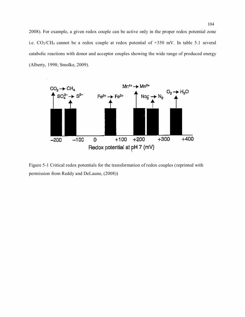
104
2008). For example, a given redox couple can be active only in the proper redox potential zone
i.e. CO2/CH4 cannot be a redox couple at redox potential of +350 mV. In table 5.1 several
catabolic reactions with donor and acceptor couples showing the wide range of produced energy
(Alberty, 1998; Smolke, 2009).
Figure 5-1 Critical redox potentials for the transformation of redox couples (reprinted with
permission from Reddy and DeLaune, (2008))
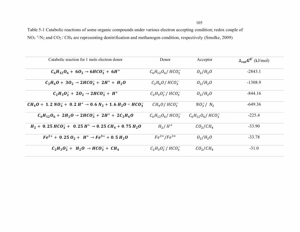
105
Table 5-1 Catabolic reactions of some organic compounds under various electron accepting condition; redox couple of
NO3 -1/N2 and CO2 / CH4 are representing denitrification and methanogen condition, respectively (Smolke, 2009)
Catabolic reaction for 1 mole electron donor Donor Acceptor ∆𝒄𝒂𝒕𝑮𝟎′
(kJ/mol)
𝑪𝟔𝑯𝟏𝟐𝑶𝟔 + 𝟔𝑶𝟐 → 𝟔𝑯𝑪𝑶𝟑− + 𝟔𝑯+ 𝐶6𝐻12𝑂6/ 𝐻𝐶𝑂3
− 𝑂2/𝐻2𝑂 -2843.1
𝑪𝟐𝑯𝟔𝑶 + 𝟑𝑶𝟐 → 𝟐𝑯𝑪𝑶𝟑− + 𝟐𝑯+ + 𝑯𝟐𝑶 𝐶2𝐻6𝑂/ 𝐻𝐶𝑂3
− 𝑂2/𝐻2𝑂 -1308.9
𝑪𝟐𝑯𝟑𝑶𝟐− + 𝟐𝑶𝟐 → 𝟐𝑯𝑪𝑶𝟑
− + 𝑯+ 𝐶2𝐻3𝑂2−/ 𝐻𝐶𝑂3
− 𝑂2/𝐻2𝑂 -844.16
𝑪𝑯𝟒𝑶 + 𝟏. 𝟐 𝑵𝑶𝟑− + 𝟎. 𝟐 𝑯+ → 𝟎.𝟔 𝑵𝟐 + 𝟏. 𝟔 𝑯𝟐𝑶 + 𝑯𝑪𝑶𝟑
− 𝐶𝐻4𝑂/ 𝐻𝐶𝑂3− 𝑁𝑂3
−/ 𝑁2 -649.36
𝑪𝟔𝑯𝟏𝟐𝑶𝟔 + 𝟐𝑯𝟐𝑶 → 𝟐𝑯𝑪𝑶𝟑− + 𝟐𝑯+ + 𝟐𝑪𝟐𝑯𝟔𝑶 𝐶6𝐻12𝑂6/ 𝐻𝐶𝑂3
− 𝐶6𝐻12𝑂6/ 𝐻𝐶𝑂3− -225.4
𝑯𝟐 + 𝟎. 𝟐𝟓 𝑯𝑪𝑶𝟑− + 𝟎. 𝟐𝟓 𝑯+ → 𝟎.𝟐𝟓 𝑪𝑯𝟒 + 𝟎. 𝟕𝟓 𝑯𝟐𝑶 𝐻2/ 𝐻
+ 𝐶𝑂2/𝐶𝐻4 -33.90
𝑭𝒆𝟐+ + 𝟎. 𝟐𝟓 𝑶𝟐 + 𝑯+ → 𝑭𝒆𝟑+ + 𝟎. 𝟓 𝑯𝟐𝑶 𝐹𝑒2+/𝐹𝑒3+ 𝑂2/𝐻2𝑂 -33.78
𝑪𝟐𝑯𝟑𝑶𝟐− + 𝑯𝟐𝑶 → 𝑯𝑪𝑶𝟑
− + 𝑪𝑯𝟒 𝐶2𝐻3𝑂2−/ 𝐻𝐶𝑂3
− 𝐶𝑂2/𝐶𝐻4 -31.0
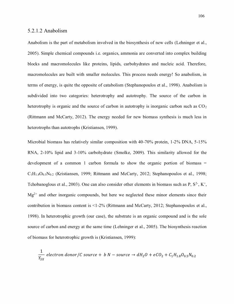
106
5.2.1.2 Anabolism
Anabolism is the part of metabolism involved in the biosynthesis of new cells (Lehninger et al.,
2005). Simple chemical compounds i.e. organics, ammonia are converted into complex building
blocks and macromolecules like proteins, lipids, carbohydrates and nucleic acid. Therefore,
macromolecules are built with smaller molecules. This process needs energy! So anabolism, in
terms of energy, is quite the opposite of catabolism (Stephanopoulos et al., 1998). Anabolism is
subdivided into two categories: heterotrophy and autotrophy. The source of the carbon in
heterotrophy is organic and the source of carbon in autotrophy is inorganic carbon such as CO2
(Rittmann and McCarty, 2012). The energy needed for new biomass synthesis is much less in
heterotrophs than autotrophs (Kristiansen, 1999).
Microbial biomass has relatively similar composition with 40-70% protein, 1-2% DNA, 5-15%
RNA, 2-10% lipid and 3-10% carbohydrate (Smolke, 2009). This similarity allowed for the
development of a common 1 carbon formula to show the organic portion of biomass =
C1H1.8O0.5N0.2 (Kristiansen, 1999; Rittmann and McCarty, 2012; Stephanopoulos et al., 1998;
Tchobanoglous et al., 2003). One can also consider other elements in biomass such as P, S2-, K+,
Mg2+ and other inorganic compounds, but here we neglected these minor elements since their
contribution in biomass content is <1-2% (Rittmann and McCarty, 2012; Stephanopoulos et al.,
1998). In heterotrophic growth (our case), the substrate is an organic compound and is the sole
source of carbon and energy at the same time (Lehninger et al., 2005). The biosynthesis reaction
of biomass for heterotrophic growth is (Kristiansen, 1999):
1
𝑌𝑆𝑋 𝑒𝑙𝑒𝑐𝑡𝑟𝑜𝑛 𝑑𝑜𝑛𝑜𝑟/𝐶 𝑠𝑜𝑢𝑟𝑐𝑒 + 𝑏 𝑁 − 𝑠𝑜𝑢𝑟𝑐𝑒 → 𝑑𝐻2𝑂 + 𝑒𝐶𝑂2 + 𝐶1𝐻1.8𝑂0.5𝑁0.2
107
In above reaction 𝑌𝑆𝑋 is the yield of substrate to biomass, b, c, d e, f, g, h are the stoichiometric
coefficients of each compound. Also, source refers to the compounds that act as the source of
carbon i.e. glucose and nitrogen source i.e. ammonia. 𝐶1𝐻1.8𝑂0.5𝑁0.2 represents the composition
of biomass. A schematic overview of metabolism is shown in Fig 5.2.
Figure 5-2 General representation of microbial metabolism. During catabolism, energy will be
produced for maintenance and growth. In anabolism the carbon source, nitrogen source and other
necessary components are used in anabolic reactions for biosynthesis of new cells.
5.2.1.3 Maintenance
In all microorganisms, damage and decay also occur i.e. protein denaturation and leakage of
molecules from membranes. These processes are commonly referred to as endogenous
metabolism: the amount of substrate that is needed at zero growth rate (Stephanopoulos et al.,
1998; Van Loosdrecht and Henze, 1999). Interestingly, it has been found that the amount of
Maintenance
108
energy needed for maintenance is similar for a broad range of microorganisms (Smolke, 2009).
These processes need to be compensated. And logically some energy must be spent! This amount
of energy (generally) has a direct relationship with temperature (approximately doubles with
every 8oC increase in temperature) (Tijhuis et al., 1993). It is interesting to mention that in the
Monod model, maintenance of the cell is not considered (Kovarova-Kovar and Egli, 1998).
5.3 Thermodynamics Background
5.3.1 Equilibrium Thermodynamics
Thermodynamics is divided into two different categories: equilibrium and non-equilibrium
(Demirel, 2014; Groot and Mazur, 1962; Smith et al., 2001). Cell growth and its metabolism take
place far or near equilibrium (Zotin, 1990). Thus, equilibrium thermodynamics fails to provide
insights into biotransformation of compounds and growth of a cell (Demirel, 2014; S. Roy
Caplan, 1983; Stephanopoulos et al., 1998; Westerhoff and Dam, 1987). Living systems are open
systems, constantly exchanging mass and energy with the environment (Roels, 1983).
The first law of thermodynamics expresses the total amount of energy in a process is constant
(Smith et al., 2001).
𝐸 = 𝑐𝑜𝑛𝑠𝑡𝑎𝑛𝑡 (5.1)
The second law of thermodynamics states that spontaneity of a process is determined from the
overall change in Gibbs free energy. Gibbs free energy (G) or free energy was introduced by
Willard Gibbs in 1878. The concept of free energy is the maximum amount of work (non-
displacement) that can be done by a system at constant pressure and temperature (Smith et al.,
2001). When ∆G < 0 the reaction is spontaneous or exogenic and the system can conduct work!
On the other hand, when ∆G > 0 the reaction (or process) is endergonic and free energy is
109
needed for the reaction to proceed. And at equilibrium, ∆G = 0 (Smith et al., 2001; Wylen et al.,
1994). For a given reaction, ∆G can be calculated (Stephanopoulos et al., 1998):
𝑎𝐴 + 𝑏𝐵 → 𝑐𝐶 + 𝑑𝐷 (5.2)
∆𝐺 = ∆𝐺0′ + 𝑅𝑇 ln (𝐶𝑐
𝑐𝐶𝐷𝑑
𝐶𝐴𝑎𝐶𝐵
𝑏) (5.3)
Where:
∆𝐺0′ = 𝑅𝑇 ln(𝐾𝑒𝑞) (5.4)
And 𝐾𝑒𝑞is:
𝐾𝑒𝑞 = 𝐶𝑐,𝑒𝑞
𝑐 𝐶𝐷,𝑒𝑞𝑑
𝐶𝐴,𝑒𝑞𝑎 𝐶𝐵,𝑒𝑞
𝑏 = 𝑒−∆𝐺0′
𝑅𝑇 (5.5)
As we mentioned above, cellular systems are open systems, which perform far from equilibrium
stage. Generally, to study non-equilibrium systems, first we investigate the system at
equilibrium, then we apply some changes to deviate the system from equilibrium (Demirel,
2014; Prigogine, 1968; Westerhoff and Dam, 1987).
5.3.2 Non-Equilibrium Thermodynamics
The mathematical foundation for non-equilibrium thermodynamics is described as follows
(Westerhoff and Dam, 1987). For context, “system” refers to a set of defined boundaries creating
separation of the system from the rest of the world. A system can interact with the outside world
through its boundaries (Smith et al., 2001; Wylen et al., 1994). These interactions can be through
(Westerhoff and Dam, 1987):
110
exchange of heat to environment (ᵭ𝑒𝑄)
pressure work carried out on the environment (ᵭ 𝑊 = −𝑝 ∙ ᵭ𝑒𝑉 )
chemical work through exchange of certain chemical (j) (∑ 𝜇𝑗𝑗 ∙ ᵭ𝑒𝑁𝑗)
mechanical work (𝐹 ∙ ᵭ𝑒𝐿)
Here, “p” represents the pressure; "𝜇𝑗" shows the chemical potential of chemical j and “F”
demonstrates the elastic force. 𝑁𝑗 , V and L are number of molecules of chemical j, volume and
length of the contractile element of the system. The notation "ᵭ" means “a small change in” and
the subscript “e” refers to the interaction with environment (out of the system’s boundaries)
(Westerhoff and Dam, 1987).
ᵭ𝑒𝐸 = ᵭ𝑒𝑄 + ᵭ 𝑊 + ∑ 𝜇𝑗
𝑗
∙ ᵭ𝑒𝑁𝑗 − 𝐹 ∙ ᵭ𝑒𝐿 (5.6)
ᵭ𝑒𝐸 = ᵭ𝑒𝑄 − 𝑝 ∙ ᵭ𝑒𝑉 + ∑𝜇𝑗
𝑗
∙ ᵭ𝑒𝑁𝑗 − 𝐹 ∙ ᵭ𝑒𝐿 (5.7)
The energy balance equation can be divided into “work” and “heat” components. The
interaction of energy with environment in terms of “work” can be described by the following
equation:
ᵭ𝑒𝑊′′ = −𝑝 ∙ ᵭ𝑒𝑉 + ∑ 𝜇𝑖
𝑚
𝑖=1
∙ ᵭ𝑒𝑚𝑖 + ∑ 𝜇𝑗
𝑛
𝑗=1
∙ ᵭ𝑒𝑛𝑗 − 𝐹 ∙ ᵭ𝑒𝐿
(5.8)
And the interaction of energy with environment in terms of “heat” can be described by the
following equation, where 𝑆�̅� is the partial molar entropy of substance j:
ᵭ𝑒𝑄′′ = ᵭ𝑒𝑄
′ + ∑ 𝑇
𝑛
𝑗=1
∙ 𝑆�̅� ∙ ᵭ𝑒𝑛𝑗 − 𝐹 ∙ ᵭ𝑒𝐿
(5.9)
111
In above equations, ᵭ𝑒𝑄′′means the pure heat exchanged (after correction for partial moral
enthalpy) and including the entropy of exchanged particles (ᵭ𝑒𝑄′ shows the heat exchanged after
correction for partial molar enthalpies of exchanged substances). The ᵭ𝑒𝑊′′demonstrates the
work including transport work (Westerhoff and Dam, 1987).
Work can be converted to heat (i.e. friction) and vice versa. To mathematically show this
balance:
ᵭ𝑒𝐸 ≝ ᵭ𝑒𝑄′′ + ᵭ𝑒𝑊
′′ (5.10)
Based on conservation of energy, we can write:
ᵭ𝐸 = ᵭ𝑒𝐸 + ᵭ𝑖𝐸 (5.11)
And due to the first law of thermodynamics, for a closed system (Smith et al., 2001; Wylen et al.,
1994):
ᵭ𝑖𝐸 = 0 (5.12)
Eq. 5.12 indicates the total amount of energy in a closed system is constant.
As we already know, ᵭ𝑒𝑄′′corresponds to heat exchanged (with environment) in the process
(through reversible processes). By dividing ᵭ𝑒𝑄′′by absolute temperature T, “entropy” is
obtained:
ᵭ𝑒𝑆 =ᵭ𝑒𝑄
′′
𝑇
(5.13)
Entropy is a state function. When a property is a state function it means, the quantity of the
property does not depend on the pathway and length of the process, it only depends on the initial
and final state of the process.
112
The second law of thermodynamics implies that for a spontaneous reaction:
ᵭ𝑒𝑆 ≥ 0 (5.14)
Where the > sign is valid for systems that are not in equilibrium and the = sign is valid for the
systems that are in equilibrium (Westerhoff and Dam, 1987).
Similar to equation 5.11:
ᵭ𝑆 = ᵭ𝑒𝑆 + ᵭ𝑖𝑆 (5.15)
ᵭ𝑆 − ᵭ𝑖𝑆 = ᵭ𝑒𝑆 (5.16)
ᵭ𝑆 − ᵭ𝑖𝑆 = ᵭ𝑒𝑆 = +ᵭ𝐸
𝑇+
𝑝
𝑇 ∙ ᵭ𝑒𝑉 − ∑
𝜇𝑖
𝑇
𝑚
𝑖=1
∙ ᵭ𝑒𝑚𝑖 − ∑𝜇𝑗
𝑇
𝑛
𝑗=1
∙ ᵭ𝑒𝑛𝑗 + 𝐹
𝑇 ∙ ᵭ𝑒𝐿
(5.17)
This equation can be re-written as:
d𝐸 = 𝑇 ∙ d𝑆 − 𝑇 ∙ ᵭ𝑖𝑆 − 𝑝 ∙ ᵭ𝑒𝑉 + ∑ 𝜇𝑖
𝑚
𝑖=1
∙ ᵭ𝑒𝑚𝑖 + ∑ 𝜇𝑗
𝑛
𝑗=1
∙ ᵭ𝑒𝑛𝑗 − 𝐹 ∙ ᵭ𝑒
(5.18)
Based on the Gibbs free energy (𝐺) definition (Smith et al., 2001):
d𝐺 ≝ d(𝐸 + 𝑝 ∙ 𝑉 − 𝑇 ∙ 𝑆) = ᵭ𝑖𝐺 + ᵭ𝑒𝐺 (5.19)
Where:
− ᵭ𝑖𝐺 ≝ + 𝑇 ∙ ᵭ𝑖𝑆 (5.20)
And
ᵭ𝑒𝐺 ≝ −𝑆 ∙ d𝑇 + 𝑉 ∙ d𝑃 + ∑ 𝜇𝑖
𝑚
𝑖=1
∙ ᵭ𝑒𝑚𝑖 + ∑ 𝜇𝑗
𝑛
𝑗=1
∙ ᵭ𝑒𝑛𝑗 − 𝐹 ∙ ᵭ𝑒𝐿
(5.21)
For a spontaneous reaction we have:
113
(d𝐺)𝑇,𝑃,𝑚𝑖,𝑛𝑗,𝐿= ᵭ𝑖𝐺 ≤ 0 (5.22)
The latter equation refers to second law of thermodynamics. The purpose of these calculation is
to provide an equation as a fundamental relationship in non-equilibrium thermodynamics.
5.3.3 Free Energy Dissipation in Spontaneous Process
To analyse a non-equilibrium situation in a real world, an example is provided. Let us assume a
chemical reaction:
𝑨 ↔ 𝑩 (5.23)
This reaction proceeds by an amount of dξ:
ᵭ𝑖𝑛𝐴 = −dξ = −ᵭ𝑖𝑛𝐵 (5.24)
However, this reaction looks reversible, we cannot use equilibrium thermodynamic approaches
to treat this reaction before it reaches equilibrium. For example, at time zero we have only
compound A. And this reaction for example needs 20 min to reach equilibrium! In this 20
minutes the reaction is not reversible (so we cannot calculate ᵭ𝑖𝐺). To simulate this reaction with
a reversible reaction we are can supply energy from the outside world (outside the system
boundary). To achieve this goal, which is having a reversible reaction, we add substance B to the
system and take the compound A out.
Therefore:
ᵭ𝑒𝑛𝐵′ = ᵭ𝑖𝑛𝐵 (5.25)
And
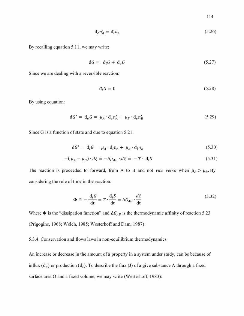
114
ᵭ𝑒𝑛𝐴′ = ᵭ𝑖𝑛𝐴 (5.26)
By recalling equation 5.11, we may write:
d𝐺 = ᵭ𝑖𝐺 + ᵭ𝑒𝐺 (5.27)
Since we are dealing with a reversible reaction:
ᵭ𝑖𝐺 = 0 (5.28)
By using equation:
d𝐺′ = ᵭ𝑒𝐺 = 𝜇𝐴 ∙ ᵭ𝑒𝑛𝐴′ + 𝜇𝐵 ∙ ᵭ𝑒𝑛𝐵
′ (5.29)
Since G is a function of state and due to equation 5.21:
d𝐺′ = ᵭ𝑖𝐺 = 𝜇𝐴 ∙ ᵭ𝑖𝑛𝐴 + 𝜇𝐵 ∙ ᵭ𝑖𝑛𝐵 (5.30)
−( 𝜇𝐴 − 𝜇𝐵) ∙ 𝑑𝜉 = −∆𝜇𝐴𝐵 ∙ 𝑑𝜉 = − 𝑇 ∙ ᵭ𝑖𝑆 (5.31)
The reaction is proceeded to forward, from A to B and not vice versa when 𝜇𝐴 > 𝜇𝐵. By
considering the role of time in the reaction:
𝚽 ≝ − ᵭ𝑖𝐺
dt= 𝑇 ∙
ᵭ𝑖𝑆
dt= ∆𝐺𝐴𝐵 ∙
𝑑𝜉
dt
(5.32)
Where 𝚽 is the “dissipation function” and ∆𝐺𝐴𝐵 is the thermodynamic affinity of reaction 5.23
(Prigogine, 1968; Welch, 1985; Westerhoff and Dam, 1987).
5.3.4. Conservation and flows laws in non-equilibrium thermodynamics
An increase or decrease in the amount of a property in a system under study, can be because of
influx (ᵭ𝑒) or production (ᵭ𝑖). To describe the flux (J) of a give substance A through a fixed
surface area O and a fixed volume, we may write (Westerhoff, 1983):
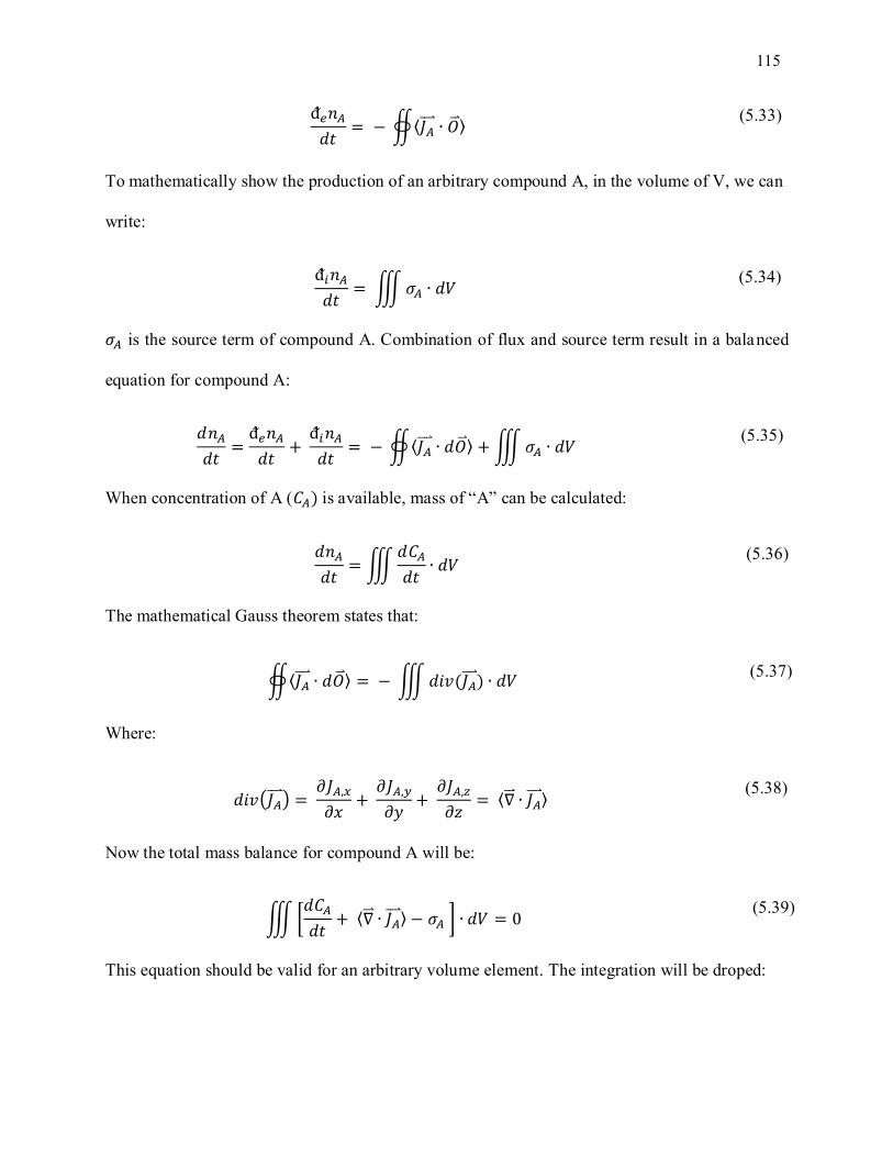
115
ᵭ𝑒𝑛𝐴
𝑑𝑡= − ∯⟨𝐽𝐴⃑⃑ ⃑ ∙ �⃑� ⟩
(5.33)
To mathematically show the production of an arbitrary compound A, in the volume of V, we can
write:
ᵭ𝑖𝑛𝐴
𝑑𝑡= ∭ 𝜎𝐴 ∙ 𝑑𝑉
(5.34)
𝜎𝐴 is the source term of compound A. Combination of flux and source term result in a balanced
equation for compound A:
𝑑𝑛𝐴
𝑑𝑡=
ᵭ𝑒𝑛𝐴
𝑑𝑡+
ᵭ𝑖𝑛𝐴
𝑑𝑡= − ∯⟨𝐽𝐴⃑⃑ ⃑ ∙ 𝑑�⃑� ⟩ + ∭ 𝜎𝐴 ∙ 𝑑𝑉
(5.35)
When concentration of A (𝐶𝐴) is available, mass of “A” can be calculated:
𝑑𝑛𝐴
𝑑𝑡= ∭
𝑑𝐶𝐴
𝑑𝑡∙ 𝑑𝑉
(5.36)
The mathematical Gauss theorem states that:
∯⟨𝐽𝐴⃑⃑ ⃑ ∙ 𝑑�⃑� ⟩ = − ∭ 𝑑𝑖𝑣(𝐽𝐴⃑⃑ ⃑) ∙ 𝑑𝑉 (5.37)
Where:
𝑑𝑖𝑣(𝐽𝐴⃑⃑ ⃑) = 𝜕𝐽𝐴,𝑥
𝜕𝑥+
𝜕𝐽𝐴,𝑦
𝜕𝑦+
𝜕𝐽𝐴,𝑧
𝜕𝑧= ⟨∇⃑⃑ ∙ 𝐽𝐴⃑⃑ ⃑⟩
(5.38)
Now the total mass balance for compound A will be:
∭ [𝑑𝐶𝐴
𝑑𝑡+ ⟨∇⃑⃑ ∙ 𝐽𝐴⃑⃑ ⃑⟩ − 𝜎𝐴 ] ∙ 𝑑𝑉 = 0
(5.39)
This equation should be valid for an arbitrary volume element. The integration will be droped:
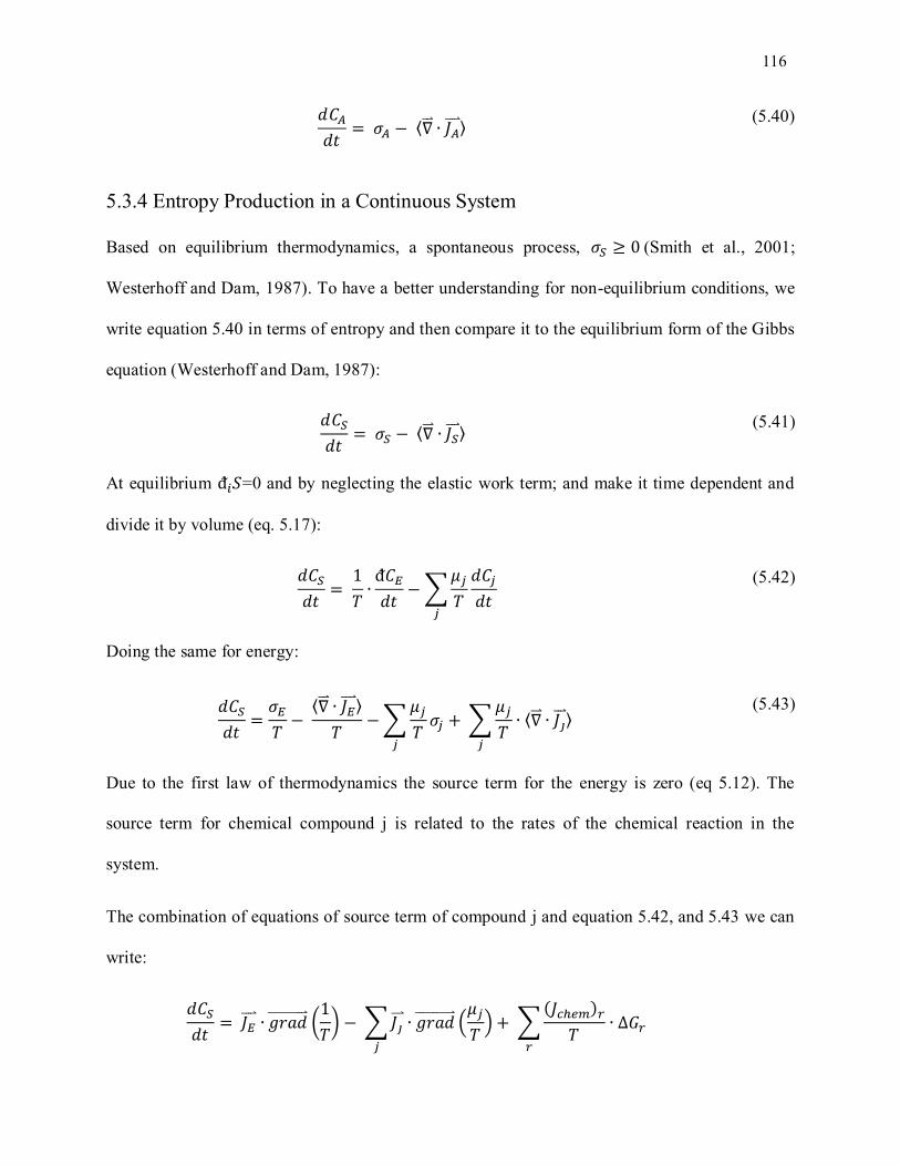
116
𝑑𝐶𝐴
𝑑𝑡= 𝜎𝐴 − ⟨∇⃑⃑ ∙ 𝐽𝐴⃑⃑ ⃑⟩
(5.40)
5.3.4 Entropy Production in a Continuous System
Based on equilibrium thermodynamics, a spontaneous process, 𝜎𝑆 ≥ 0 (Smith et al., 2001;
Westerhoff and Dam, 1987). To have a better understanding for non-equilibrium conditions, we
write equation 5.40 in terms of entropy and then compare it to the equilibrium form of the Gibbs
equation (Westerhoff and Dam, 1987):
𝑑𝐶𝑆
𝑑𝑡= 𝜎𝑆 − ⟨∇⃑⃑ ∙ 𝐽𝑆⃑⃑⃑ ⟩
(5.41)
At equilibrium ᵭ𝑖𝑆=0 and by neglecting the elastic work term; and make it time dependent and
divide it by volume (eq. 5.17):
𝑑𝐶𝑆
𝑑𝑡=
1
𝑇∙ᵭ𝐶𝐸
𝑑𝑡− ∑
𝜇𝑗
𝑇𝑗
𝑑𝐶𝑗
𝑑𝑡
(5.42)
Doing the same for energy:
𝑑𝐶𝑆
𝑑𝑡=
𝜎𝐸
𝑇−
⟨∇⃑⃑ ∙ 𝐽𝐸⃑⃑ ⃑⟩
𝑇− ∑
𝜇𝑗
𝑇𝑗
𝜎𝑗 + ∑𝜇𝑗
𝑇𝑗
∙ ⟨∇⃑⃑ ∙ 𝐽𝑗⃑⃑ ⟩ (5.43)
Due to the first law of thermodynamics the source term for the energy is zero (eq 5.12). The
source term for chemical compound j is related to the rates of the chemical reaction in the
system.
The combination of equations of source term of compound j and equation 5.42, and 5.43 we can
write:
𝑑𝐶𝑆
𝑑𝑡= 𝐽𝐸⃑⃑ ⃑ ∙ 𝑔𝑟𝑎𝑑⃑⃑⃑⃑ ⃑⃑ ⃑⃑ ⃑⃑ (
1
𝑇) − ∑𝐽𝑗⃑⃑
𝑗
∙ 𝑔𝑟𝑎𝑑⃑⃑⃑⃑ ⃑⃑ ⃑⃑ ⃑⃑ (𝜇𝑗
𝑇) + ∑
(𝐽𝑐ℎ𝑒𝑚)𝑟
𝑇𝑟
∙ ∆𝐺𝑟
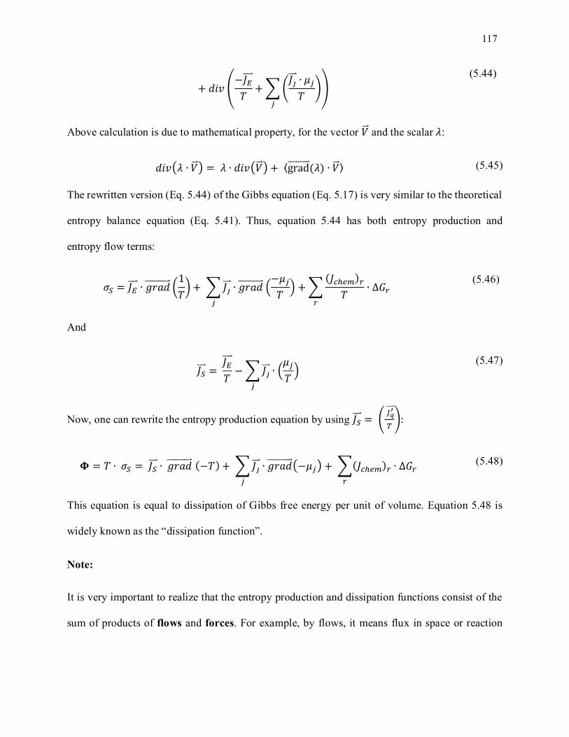
117
+ 𝑑𝑖𝑣 (−𝐽𝐸⃑⃑ ⃑
𝑇+ ∑ (
𝐽𝑗⃑⃑ ∙ 𝜇𝑗
𝑇)
𝑗
)
(5.44)
Above calculation is due to mathematical property, for the vector �⃑� and the scalar 𝜆:
𝑑𝑖𝑣(𝜆 ∙ �⃑� ) = 𝜆 ∙ 𝑑𝑖𝑣(�⃑� ) + ⟨grad⃑⃑⃑⃑⃑⃑ ⃑⃑ ⃑(𝜆) ∙ �⃑� ⟩ (5.45)
The rewritten version (Eq. 5.44) of the Gibbs equation (Eq. 5.17) is very similar to the theoretical
entropy balance equation (Eq. 5.41). Thus, equation 5.44 has both entropy production and
entropy flow terms:
𝜎𝑆 = 𝐽𝐸⃑⃑ ⃑ ∙ 𝑔𝑟𝑎𝑑⃑⃑⃑⃑ ⃑⃑ ⃑⃑ ⃑⃑ (1
𝑇) + ∑ 𝐽𝑗⃑⃑
𝑗
∙ 𝑔𝑟𝑎𝑑⃑⃑⃑⃑ ⃑⃑ ⃑⃑ ⃑⃑ (−𝜇𝑗
𝑇) + ∑
(𝐽𝑐ℎ𝑒𝑚)𝑟
𝑇𝑟
∙ ∆𝐺𝑟 (5.46)
And
𝐽𝑆⃑⃑⃑ = 𝐽𝐸⃑⃑ ⃑
𝑇− ∑ 𝐽𝑗⃑⃑
𝑗
∙ (𝜇𝑗
𝑇)
(5.47)
Now, one can rewrite the entropy production equation by using 𝐽𝑆⃑⃑⃑ = ( 𝐽𝑞
′⃑⃑⃑⃑
𝑇):
𝚽 = 𝑇 ∙ 𝜎𝑆 = 𝐽𝑆⃑⃑⃑ ∙ 𝑔𝑟𝑎𝑑⃑⃑⃑⃑ ⃑⃑ ⃑⃑ ⃑⃑ (−𝑇) + ∑ 𝐽𝑗⃑⃑
𝑗
∙ 𝑔𝑟𝑎𝑑⃑⃑⃑⃑ ⃑⃑ ⃑⃑ ⃑⃑ (−𝜇𝑗) + ∑(𝐽𝑐ℎ𝑒𝑚)𝑟𝑟
∙ ∆𝐺𝑟 (5.48)
This equation is equal to dissipation of Gibbs free energy per unit of volume. Equation 5.48 is
widely known as the “dissipation function”.
Note:
It is very important to realize that the entropy production and dissipation functions consist of the
sum of products of flows and forces. For example, by flows, it means flux in space or reaction
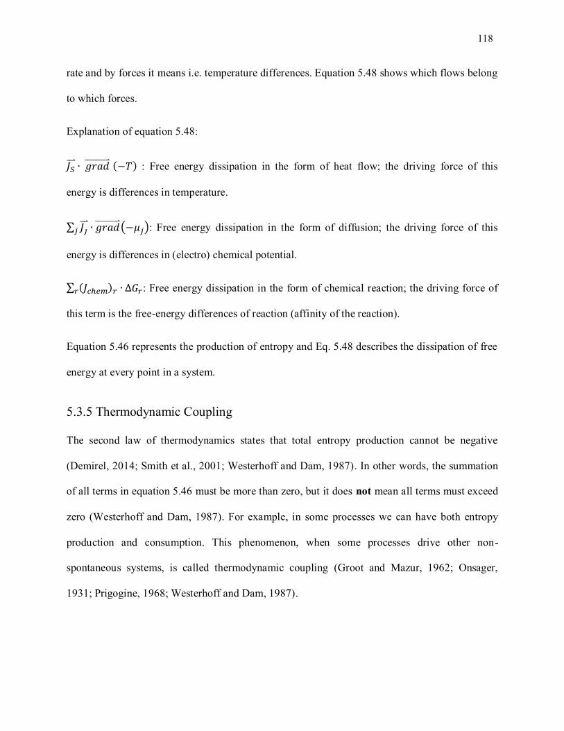
118
rate and by forces it means i.e. temperature differences. Equation 5.48 shows which flows belong
to which forces.
Explanation of equation 5.48:
𝐽𝑆⃑⃑⃑ ∙ 𝑔𝑟𝑎𝑑⃑⃑⃑⃑ ⃑⃑ ⃑⃑ ⃑⃑ (−𝑇) : Free energy dissipation in the form of heat flow; the driving force of this
energy is differences in temperature.
∑ 𝐽𝑗⃑⃑ 𝑗 ∙ 𝑔𝑟𝑎𝑑⃑⃑⃑⃑ ⃑⃑ ⃑⃑ ⃑⃑ (−𝜇𝑗): Free energy dissipation in the form of diffusion; the driving force of this
energy is differences in (electro) chemical potential.
∑ (𝐽𝑐ℎ𝑒𝑚)𝑟𝑟 ∙ ∆𝐺𝑟: Free energy dissipation in the form of chemical reaction; the driving force of
this term is the free-energy differences of reaction (affinity of the reaction).
Equation 5.46 represents the production of entropy and Eq. 5.48 describes the dissipation of free
energy at every point in a system.
5.3.5 Thermodynamic Coupling
The second law of thermodynamics states that total entropy production cannot be negative
(Demirel, 2014; Smith et al., 2001; Westerhoff and Dam, 1987). In other words, the summation
of all terms in equation 5.46 must be more than zero, but it does not mean all terms must exceed
zero (Westerhoff and Dam, 1987). For example, in some processes we can have both entropy
production and consumption. This phenomenon, when some processes drive other non-
spontaneous systems, is called thermodynamic coupling (Groot and Mazur, 1962; Onsager,
1931; Prigogine, 1968; Westerhoff and Dam, 1987).
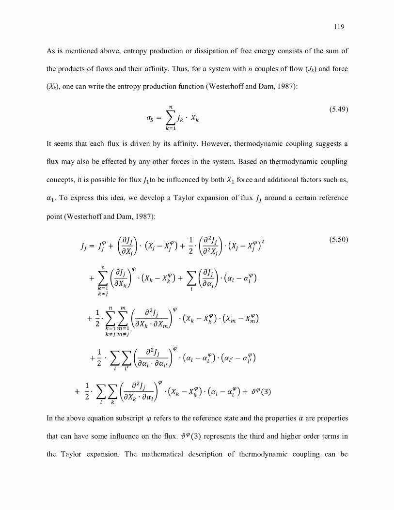
119
As is mentioned above, entropy production or dissipation of free energy consists of the sum of
the products of flows and their affinity. Thus, for a system with n couples of flow (Jk) and force
(Xk), one can write the entropy production function (Westerhoff and Dam, 1987):
𝜎𝑆 = ∑ 𝐽𝑘 ∙ 𝑋𝑘
𝑛
𝑘=1
(5.49)
It seems that each flux is driven by its affinity. However, thermodynamic coupling suggests a
flux may also be effected by any other forces in the system. Based on thermodynamic coupling
concepts, it is possible for flux 𝐽1to be influenced by both 𝑋1 force and additional factors such as,
𝛼1. To express this idea, we develop a Taylor expansion of flux 𝐽𝑗 around a certain reference
point (Westerhoff and Dam, 1987):
𝐽𝑗 = 𝐽𝑗𝜑
+ (𝜕𝐽𝑗
𝜕𝑋𝑗
) ∙ (𝑋𝑗 − 𝑋𝑗𝜑) +
1
2∙ (
𝜕2𝐽𝑗
𝜕2𝑋𝑗
) ∙ (𝑋𝑗 − 𝑋𝑗𝜑)2
+ ∑ (𝜕𝐽𝑗
𝜕𝑋𝑘
)
𝜑
∙
𝑛
𝑘=1𝑘≠𝑗
(𝑋𝑘 − 𝑋𝑘𝜑) + ∑(
𝜕𝐽𝑗
𝜕𝛼𝑙
)
𝑙
∙ (𝛼𝑙 − 𝛼𝑙𝜑)
+ 1
2∙ ∑ ∑ (
𝜕2𝐽𝑗
𝜕𝑋𝑘 ∙ 𝜕𝑋𝑚)
𝜑
∙ (𝑋𝑘 − 𝑋𝑘𝜑) ∙ (𝑋𝑚 − 𝑋𝑚
𝜑)
𝑚
𝑚=1𝑚≠𝑗
𝑛
𝑘=1𝑘≠𝑗
+1
2 ∙ ∑ ∑ (
𝜕2𝐽𝑗
𝜕𝛼𝑙 ∙ 𝜕𝛼𝑙′)
𝜑
𝑙′𝑙
∙ (𝛼𝑙 − 𝛼𝑙𝜑) ∙ (𝛼𝑙′ − 𝛼
𝑙′𝜑)
+ 1
2∙ ∑ ∑ (
𝜕2𝐽𝑗
𝜕𝑋𝑘 ∙ 𝜕𝛼𝑙)
𝜑
∙
𝑘𝑙
(𝑋𝑘 − 𝑋𝑘𝜑) ∙ (𝛼𝑙 − 𝛼𝑙
𝜑) + 𝜗𝜑(3)
(5.50)
In the above equation subscript 𝜑 refers to the reference state and the properties 𝛼 are properties
that can have some influence on the flux. 𝜗𝜑(3) represents the third and higher order terms in
the Taylor expansion. The mathematical description of thermodynamic coupling can be
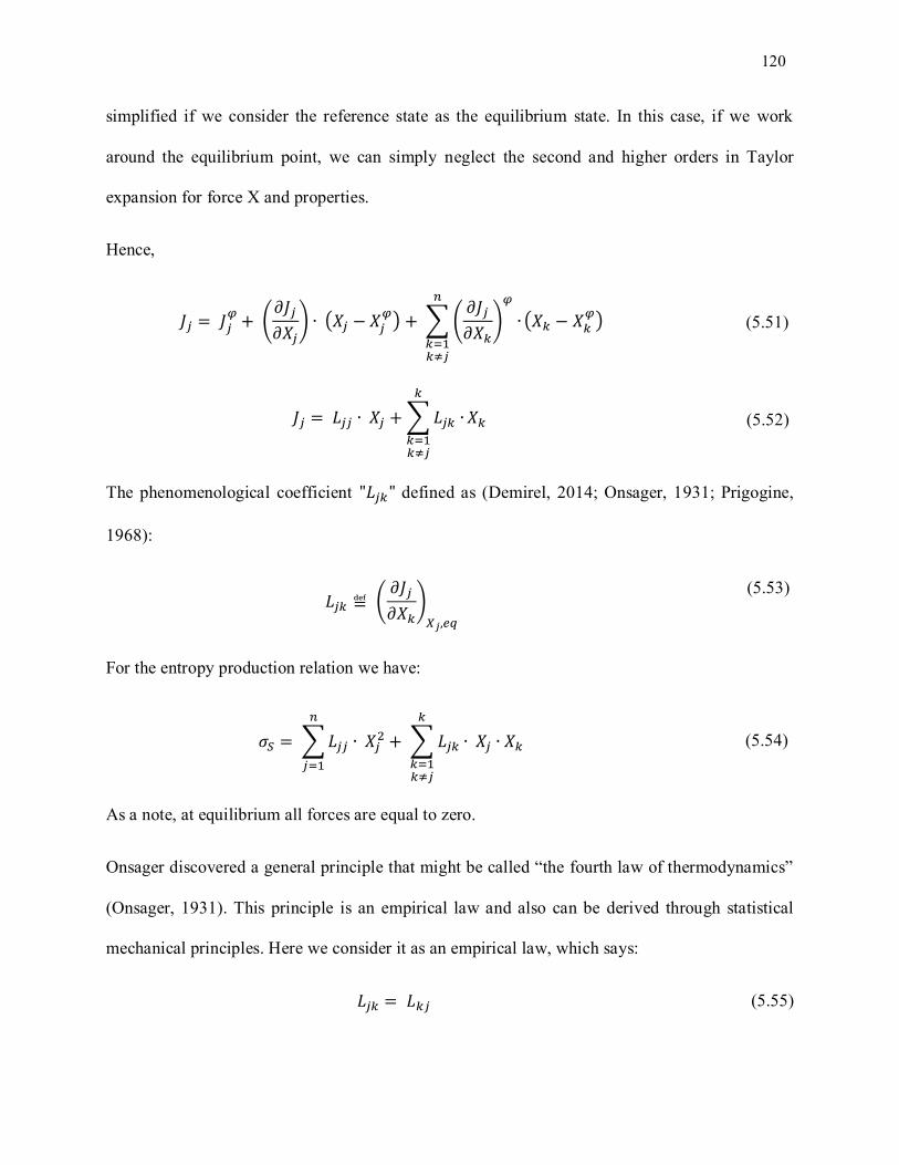
120
simplified if we consider the reference state as the equilibrium state. In this case, if we work
around the equilibrium point, we can simply neglect the second and higher orders in Taylor
expansion for force X and properties.
Hence,
𝐽𝑗 = 𝐽𝑗𝜑
+ (𝜕𝐽𝑗
𝜕𝑋𝑗
) ∙ (𝑋𝑗 − 𝑋𝑗𝜑) + ∑ (
𝜕𝐽𝑗
𝜕𝑋𝑘
)
𝜑
∙
𝑛
𝑘=1𝑘≠𝑗
(𝑋𝑘 − 𝑋𝑘𝜑)
(5.51)
𝐽𝑗 = 𝐿𝑗𝑗 ∙ 𝑋𝑗 + ∑ 𝐿𝑗𝑘 ∙
𝑘
𝑘=1𝑘≠𝑗
𝑋𝑘
(5.52)
The phenomenological coefficient "𝐿𝑗𝑘" defined as (Demirel, 2014; Onsager, 1931; Prigogine,
1968):
𝐿𝑗𝑘 ≝ (𝜕𝐽𝑗
𝜕𝑋𝑘)
𝑋𝑗,𝑒𝑞
(5.53)
For the entropy production relation we have:
𝜎𝑆 = ∑𝐿𝑗𝑗 ∙ 𝑋𝑗2
𝑛
𝑗=1
+ ∑ 𝐿𝑗𝑘 ∙ 𝑋𝑗 ∙ 𝑋𝑘
𝑘
𝑘=1𝑘≠𝑗
(5.54)
As a note, at equilibrium all forces are equal to zero.
Onsager discovered a general principle that might be called “the fourth law of thermodynamics”
(Onsager, 1931). This principle is an empirical law and also can be derived through statistical
mechanical principles. Here we consider it as an empirical law, which says:
𝐿𝑗𝑘 = 𝐿𝑘𝑗 (5.55)
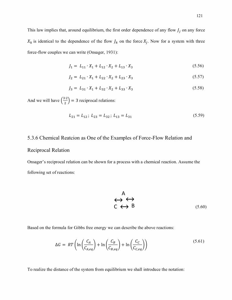
121
This law implies that, around equilibrium, the first order dependence of any flow 𝐽𝑗 on any force
𝑋𝑘 is identical to the dependence of the flow 𝐽𝑘 on the force 𝑋𝑗 . Now for a system with three
force-flow couples we can write (Onsager, 1931):
𝐽1 = 𝐿11 ∙ 𝑋1 + 𝐿12 ∙ 𝑋2 + 𝐿13 ∙ 𝑋3 (5.56)
𝐽2 = 𝐿21 ∙ 𝑋1 + 𝐿22 ∙ 𝑋2 + 𝐿23 ∙ 𝑋3 (5.57)
𝐽3 = 𝐿31 ∙ 𝑋1 + 𝐿32 ∙ 𝑋2 + 𝐿33 ∙ 𝑋3 (5.58)
And we will have (3∙2
2) = 3 reciprocal relations:
𝐿21 = 𝐿12 ; 𝐿23 = 𝐿32 ; 𝐿13 = 𝐿31 (5.59)
5.3.6 Chemical Reatcion as One of the Examples of Force-Flow Relation and
Reciprocal Relation
Onsager’s reciprocal relation can be shown for a process with a chemical reaction. Assume the
following set of reactions:
(5.60)
Based on the formula for Gibbs free energy we can describe the above reactions:
∆𝐺 = 𝑅𝑇 (ln (𝐶𝐴
𝐶𝐴,𝑒𝑞) + ln (
𝐶𝐵
𝐶𝐵,𝑒𝑞) + ln (
𝐶𝐶
𝐶𝐶,𝑒𝑞))
(5.61)
To realize the distance of the system from equilibrium we shall introduce the notation:
↔ ↔ A
↔ B C
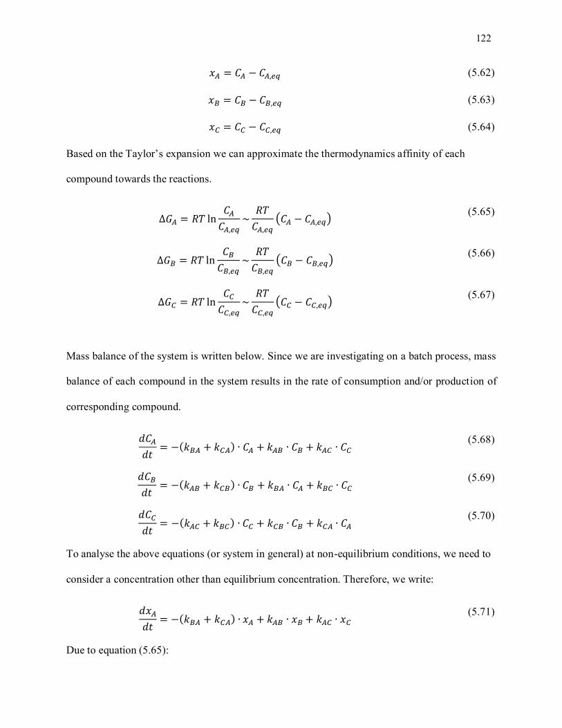
122
𝑥𝐴 = 𝐶𝐴 − 𝐶𝐴,𝑒𝑞 (5.62)
𝑥𝐵 = 𝐶𝐵 − 𝐶𝐵,𝑒𝑞 (5.63)
𝑥𝐶 = 𝐶𝐶 − 𝐶𝐶,𝑒𝑞 (5.64)
Based on the Taylor’s expansion we can approximate the thermodynamics affinity of each
compound towards the reactions.
∆𝐺𝐴 = 𝑅𝑇 ln𝐶𝐴
𝐶𝐴,𝑒𝑞
~𝑅𝑇
𝐶𝐴,𝑒𝑞
(𝐶𝐴 − 𝐶𝐴,𝑒𝑞) (5.65)
∆𝐺𝐵 = 𝑅𝑇 ln𝐶𝐵
𝐶𝐵,𝑒𝑞~
𝑅𝑇
𝐶𝐵,𝑒𝑞
(𝐶𝐵 − 𝐶𝐵,𝑒𝑞) (5.66)
∆𝐺𝐶 = 𝑅𝑇 ln𝐶𝐶
𝐶𝐶,𝑒𝑞
~𝑅𝑇
𝐶𝐶,𝑒𝑞
(𝐶𝐶 − 𝐶𝐶,𝑒𝑞) (5.67)
Mass balance of the system is written below. Since we are investigating on a batch process, mass
balance of each compound in the system results in the rate of consumption and/or production of
corresponding compound.
𝑑𝐶𝐴
𝑑𝑡= −(𝑘𝐵𝐴 + 𝑘𝐶𝐴) ∙ 𝐶𝐴 + 𝑘𝐴𝐵 ∙ 𝐶𝐵 + 𝑘𝐴𝐶 ∙ 𝐶𝐶
(5.68)
𝑑𝐶𝐵
𝑑𝑡= −(𝑘𝐴𝐵 + 𝑘𝐶𝐵) ∙ 𝐶𝐵 + 𝑘𝐵𝐴 ∙ 𝐶𝐴 + 𝑘𝐵𝐶 ∙ 𝐶𝐶
(5.69)
𝑑𝐶𝐶
𝑑𝑡= −(𝑘𝐴𝐶 + 𝑘𝐵𝐶) ∙ 𝐶𝐶 + 𝑘𝐶𝐵 ∙ 𝐶𝐵 + 𝑘𝐶𝐴 ∙ 𝐶𝐴
(5.70)
To analyse the above equations (or system in general) at non-equilibrium conditions, we need to
consider a concentration other than equilibrium concentration. Therefore, we write:
𝑑𝑥𝐴
𝑑𝑡= −(𝑘𝐵𝐴 + 𝑘𝐶𝐴) ∙ 𝑥𝐴 + 𝑘𝐴𝐵 ∙ 𝑥𝐵 + 𝑘𝐴𝐶 ∙ 𝑥𝐶
(5.71)
Due to equation (5.65):
123
(𝐶𝐴 − 𝐶𝐴,𝑒𝑞) = 𝑥𝐴 =𝐶𝐴,𝑒𝑞
𝑅𝑇∙ ∆𝐺𝐴
(5.72)
So for equation (5.71) we have:
𝑑𝑥𝐴
𝑑𝑡= −(𝑘𝐵𝐴 + 𝑘𝐶𝐴) ∙
𝐶𝐴,𝑒𝑞
𝑅𝑇∙ ∆𝐺𝐴 + 𝑘𝐴𝐵 ∙
𝐶𝐵,𝑒𝑞
𝑅𝑇∙ ∆𝐺𝐵 + 𝑘𝐴𝐶 ∙
𝐶𝐶,𝑒𝑞
𝑅𝑇∙ ∆𝐺𝐶
(5.73)
𝑑𝑥𝐵
𝑑𝑡= −(𝑘𝐴𝐵 + 𝑘𝐶𝐵) ∙
𝐶𝐵,𝑒𝑞
𝑅𝑇∙ ∆𝐺𝐵 + 𝑘𝐵𝐴 ∙
𝐶𝐴,𝑒𝑞
𝑅𝑇∙ ∆𝐺𝐴 + 𝑘𝐵𝐶 ∙
𝐶𝐶,𝑒𝑞
𝑅𝑇∙ ∆𝐺𝐶
(5.74)
𝑑𝑥𝐶
𝑑𝑡= −(𝑘𝐴𝐶 + 𝑘𝐵𝐶) ∙
𝐶𝐶,𝑒𝑞
𝑅𝑇∙ ∆𝐺𝐶 + 𝑘𝐶𝐵 ∙
𝐶𝐵,𝑒𝑞
𝑅𝑇∙ ∆𝐺𝐵 + 𝑘𝐶𝐴 ∙
𝐶𝐴,𝑒𝑞
𝑅𝑇∙ ∆𝐺𝐴
(5.75)
By comparison equations (5.73) to equation (5.76), the analogy between equation terms can be
seen. Comparison is as follows:
𝐽𝐴 = 𝐿11 ∙ 𝑋1 + 𝐿12 ∙ 𝑋2 + 𝐿13 ∙ 𝑋3 (5.76)
For compound A, we have:
𝐿11 = −(𝑘𝐵𝐴 + 𝑘𝐶𝐴) ∙𝐶𝐴,𝑒𝑞
𝑅𝑇 ; 𝑋1 = ∆𝐺𝐴
(5.77)
𝐿12 = 𝑘𝐴𝐵 ∙𝐶𝐵,𝑒𝑞
𝑅𝑇; 𝑋2 = ∆𝐺𝐵
(5.78)
𝐿13 = 𝑘𝐴𝐶 ∙𝐶𝐶,𝑒𝑞
𝑅𝑇; 𝑋3 = ∆𝐺𝐶
(5.79)
And one can show the reciprocal relations in this process. For example, for 𝐿13 = 𝐿31we can
compare these two relationships:
𝐿13 = 𝑘𝐴𝐶 ∙𝐶𝐶,𝑒𝑞
𝑅𝑇
(5.80)
𝐿31 = 𝑘𝐶𝐴 ∙𝐶𝐴,𝑒𝑞
𝑅𝑇
(5.81)
𝑘𝐴𝐶 ∙𝐶𝐶,𝑒𝑞
𝑅𝑇= 𝑘𝐶𝐴 ∙
𝐶𝐴,𝑒𝑞
𝑅𝑇
(5.82)
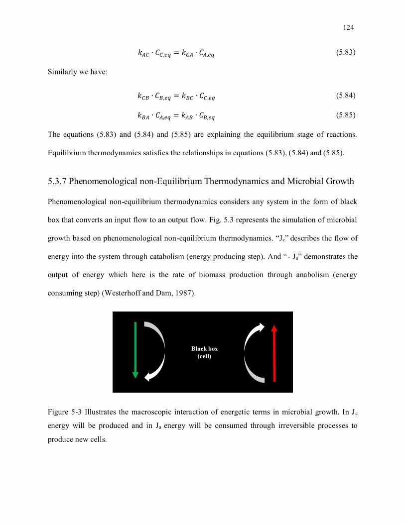
124
𝑘𝐴𝐶 ∙ 𝐶𝐶,𝑒𝑞 = 𝑘𝐶𝐴 ∙ 𝐶𝐴,𝑒𝑞 (5.83)
Similarly we have:
𝑘𝐶𝐵 ∙ 𝐶𝐵,𝑒𝑞 = 𝑘𝐵𝐶 ∙ 𝐶𝐶,𝑒𝑞 (5.84)
𝑘𝐵𝐴 ∙ 𝐶𝐴,𝑒𝑞 = 𝑘𝐴𝐵 ∙ 𝐶𝐵,𝑒𝑞 (5.85)
The equations (5.83) and (5.84) and (5.85) are explaining the equilibrium stage of reactions.
Equilibrium thermodynamics satisfies the relationships in equations (5.83), (5.84) and (5.85).
5.3.7 Phenomenological non-Equilibrium Thermodynamics and Microbial Growth
Phenomenological non-equilibrium thermodynamics considers any system in the form of black
box that converts an input flow to an output flow. Fig. 5.3 represents the simulation of microbial
growth based on phenomenological non-equilibrium thermodynamics. “Jc” describes the flow of
energy into the system through catabolism (energy producing step). And “- Ja” demonstrates the
output of energy which here is the rate of biomass production through anabolism (energy
consuming step) (Westerhoff and Dam, 1987).
Figure 5-3 Illustrates the macroscopic interaction of energetic terms in microbial growth. In Jc
energy will be produced and in Ja energy will be consumed through irreversible processes to
produce new cells.
125
By implementing the Onsager reciprocal relation, one can describe the flow and forces for the
microbial growth system (Westerhoff and Dam, 1987):
𝐽𝑐 = 𝐿𝑐𝑐 ∙ (∆𝐺𝑐 − ∆𝐺𝑐#) + 𝐿𝑐𝑎 ∙ (∆𝐺𝑎 − ∆𝐺𝑎
#) (5.86)
𝐽𝑎 = 𝐿𝑎𝑐 ∙ (∆𝐺𝑐 − ∆𝐺𝑐#) + 𝐿𝑎𝑎 ∙ (∆𝐺𝑎 − ∆𝐺𝑎
#) (5.87)
In the above equations, ∆𝐺𝑐 and ∆𝐺𝑎 are free energy differences for catabolism and anabolism
respectively and ∆𝐺𝑐# and ∆𝐺𝑎
# are independent constants. If we write equations 5.86 and 5.87 at
the equilibrium point, ∆𝐺𝑐# = ∆𝐺𝑎
# = 0:
𝐽𝑐 = 𝐿𝑐𝑐 ∙ ∆𝐺𝑐 + 𝐿𝑐𝑎 ∙ ∆𝐺𝑎 (5.88)
𝐽𝑎 = 𝐿𝑎𝑐 ∙ ∆𝐺𝑐 + 𝐿𝑎𝑎 ∙ ∆𝐺𝑎
(5.89)
Equation (5.88) represents the flux of catabolism and equation (5.89) shows the flux of anabolic
reactions. To describe the total substrate flux we can sum these two equations:
𝐽𝑠 = 𝐽𝑐 + (−𝐽𝑎) (5.90)
𝐽𝑠 = ∆𝐺𝑐 (𝐿𝑐𝑐 − 𝐿𝑎𝑐) + ∆𝐺𝑎 (𝐿𝑐𝑎 − 𝐿𝑎𝑎) (5.91)
∆𝐺𝑐 can be written based on equation (5.88). By replacing ∆𝐺𝑐 from equation (5.88) and put it
into equation (5.91), following equation is obtained:
𝐽𝑠 = ((𝐿𝑐𝑎 − 𝐿𝑐𝑐
𝐿𝑎𝑐) ∙ (−𝐽𝑎)) − (∆𝐺𝑎 ∙ ((𝐿𝑐𝑐 − 𝐿𝑎𝑐) ∙ (
𝐿𝑎𝑎
𝐿𝑎𝑐) + (𝐿𝑐𝑎 − 𝐿𝑎𝑎)))
(5.92)
We can also represent the above linear equation in this format (Westerhoff and Dam, 1987):
𝐽𝑠 = 𝛼 ∙ (−𝐽𝑎) + 𝛽 (5.93)
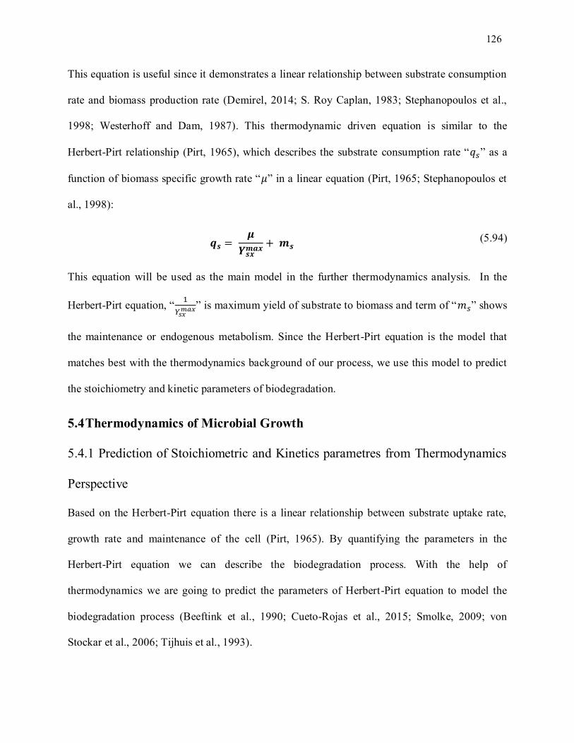
126
This equation is useful since it demonstrates a linear relationship between substrate consumption
rate and biomass production rate (Demirel, 2014; S. Roy Caplan, 1983; Stephanopoulos et al.,
1998; Westerhoff and Dam, 1987). This thermodynamic driven equation is similar to the
Herbert-Pirt relationship (Pirt, 1965), which describes the substrate consumption rate “𝑞𝑠” as a
function of biomass specific growth rate “𝜇” in a linear equation (Pirt, 1965; Stephanopoulos et
al., 1998):
𝒒𝒔 = 𝝁
𝒀𝒔𝒙𝒎𝒂𝒙
+ 𝒎𝒔 (5.94)
This equation will be used as the main model in the further thermodynamics analysis. In the
Herbert-Pirt equation, “1
𝑌𝑠𝑥𝑚𝑎𝑥” is maximum yield of substrate to biomass and term of “𝑚𝑠” shows
the maintenance or endogenous metabolism. Since the Herbert-Pirt equation is the model that
matches best with the thermodynamics background of our process, we use this model to predict
the stoichiometry and kinetic parameters of biodegradation.
5.4 Thermodynamics of Microbial Growth
5.4.1 Prediction of Stoichiometric and Kinetics parametres from Thermodynamics
Perspective
Based on the Herbert-Pirt equation there is a linear relationship between substrate uptake rate,
growth rate and maintenance of the cell (Pirt, 1965). By quantifying the parameters in the
Herbert-Pirt equation we can describe the biodegradation process. With the help of
thermodynamics we are going to predict the parameters of Herbert-Pirt equation to model the
biodegradation process (Beeftink et al., 1990; Cueto-Rojas et al., 2015; Smolke, 2009; von
Stockar et al., 2006; Tijhuis et al., 1993).
127
5.4.1.1 Prediction of Substrate Needed for Maintenance
Even at zero growth rate, cells need to spend energy to support their life through maintenance
processes (Stephanopoulos et al., 1998). Maintenance energy was found to be independent of
substrate (carbon source) and nitrogen source (Heijnen et al., 1992; Tijhuis et al., 1993).
However, as mentioned in section (5.2.1.3) temperature is the most significant factor in
determining maintenance energy (Beeftink et al., 1990; Tijhuis et al., 1993). This amount of
energy mG is expressed in kJ of Gibbs free energy per 1 C-mole of biomass (C1H1.8O0.9N0.2) per
hour (Beeftink et al., 1990; Tijhuis et al., 1993). The difference in maintenance energy under
aerobic and anaerobic conditions are not significant (Heijnen, 2010; Tijhuis et al., 1993). Fig. 5.4
shows the correlation between mG and temperature under aerobic and anaerobic conditions.
5.4.1.1.1 Required Substrate for Maintenance
We know that the source of energy for maintenance is the catabolic reaction. ∆Gcat has units of
kJ per mole substrate and mG has units of kJ per C-moleCx per hour.
Hence:
𝑚𝑆 = 𝑚𝐺
∆𝐺𝑐𝑎𝑡 [
𝑘𝐽𝐶 − 𝑚𝑜𝑙𝑒𝑋. ℎ
𝑘𝐽𝑚𝑜𝑙𝑒 𝑆
]
(5.95)
𝑚𝑆 = 𝑚𝐺
∆𝐺𝑐𝑎𝑡 [
𝑚𝑜𝑙𝑒 𝑆
𝐶 − 𝑚𝑜𝑙𝑒𝑋. ℎ]
(5.96)
Where ms shows the amount of needed substrate for maintenance. Based on this formula (Eq.
5.97), one can calculate the needed substrate for cell maintenance (Colin Ratledge, 2006;
Heijnen, 2010; Smolke, 2009).
128
5.4.1.1.2 Required Energy for Maintenance
To calculate the maintenance energy (mG) based on the above correlations (Colin Ratledge,
2006; Heijnen, 2010; Smolke, 2009; Tijhuis et al., 1993), following equation is proposed:
𝑚𝐺 = 4.5 𝑒𝑥𝑝 [−69000
𝑅(1
𝑇−
1
298)] [
𝑘𝐽
𝐶 − 𝑚𝑜𝑙𝑒𝐶𝑥. ℎ]
(5.97)
In this equation:
R: is universal gas constant 8.314 J mole-1 K-1
T: is absolute temperature
mG: is maintenance Gibbs free energy kJ h-1 C-mole𝐶𝑥-1
This equation tells us that at standard condition (T=25 oC), in one hour, one C-mole of the cell
needs 4.5 kJ energy at least to survive. However, theses correlations have the confidence
interval of 41% for aerobic growth and 47% for anaerobic growth. The accuracy of proposed
equation is not high, however, up to date, it has been the only equation that proposed and used
widely in biotechnology and environmental biotechnology purposes.
129
Figure 5-4 There is 41% accuracy (aerobic growth) for prediction of maintenance energy based
on Eq. 5.97 and 47% accuracy for anaerobic growth (reprinted with permission from Tijhuis et
al., (1993)).
The amount of maintenance energy comes from the catabolism of electron donor. Now based on
the type of the electron donor and acceptor we can calculate the required amount of substrate
needed to supply maintenance energy (Colin Ratledge, 2006; Heijnen, 2010).
5.4.1.2 Prediction of Gibbs Energy Needed for Growth
“1
𝑌𝑆𝑋𝑚𝑎𝑥” is a stoichiometric parameter that shows us the amount of consumed substrate for
biosynthesis of 1 C-mole biomass. This stoichiometric parameter is equal to the amount of
energy needed for biosynthesis of biomass (1
𝑌𝐺𝑋𝑚𝑎𝑥) (Heijnen, 2010; Roels, 1983; Urs von
Stockar, 2013). This amount of energy represents the amount of biochemical work required to
produce biomass from an available C-source through irreversible carbon-carbon coupling and
oxidation/reduction reactions. Therefore, dissipation energy greatly depends on two main
properties of a carbon source (Heijnen and Van Dijken, 1992):
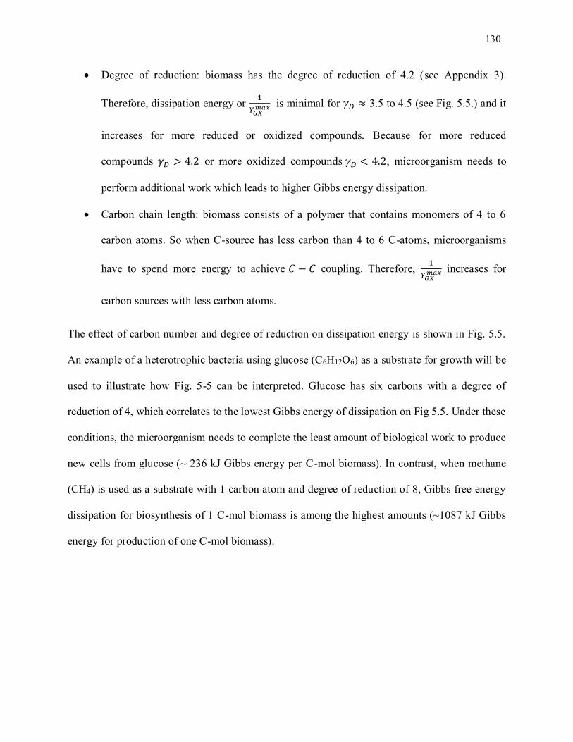
130
Degree of reduction: biomass has the degree of reduction of 4.2 (see Appendix 3).
Therefore, dissipation energy or 1
𝑌𝐺𝑋𝑚𝑎𝑥 is minimal for 𝛾𝐷 ≈ 3.5 to 4.5 (see Fig. 5.5.) and it
increases for more reduced or oxidized compounds. Because for more reduced
compounds 𝛾𝐷 > 4.2 or more oxidized compounds 𝛾𝐷 < 4.2, microorganism needs to
perform additional work which leads to higher Gibbs energy dissipation.
Carbon chain length: biomass consists of a polymer that contains monomers of 4 to 6
carbon atoms. So when C-source has less carbon than 4 to 6 C-atoms, microorganisms
have to spend more energy to achieve 𝐶 − 𝐶 coupling. Therefore, 1
𝑌𝐺𝑋𝑚𝑎𝑥 increases for
carbon sources with less carbon atoms.
The effect of carbon number and degree of reduction on dissipation energy is shown in Fig. 5.5.
An example of a heterotrophic bacteria using glucose (C6H12O6) as a substrate for growth will be
used to illustrate how Fig. 5-5 can be interpreted. Glucose has six carbons with a degree of
reduction of 4, which correlates to the lowest Gibbs energy of dissipation on Fig 5.5. Under these
conditions, the microorganism needs to complete the least amount of biological work to produce
new cells from glucose (~ 236 kJ Gibbs energy per C-mol biomass). In contrast, when methane
(CH4) is used as a substrate with 1 carbon atom and degree of reduction of 8, Gibbs free energy
dissipation for biosynthesis of 1 C-mol biomass is among the highest amounts (~1087 kJ Gibbs
energy for production of one C-mol biomass).
131
Figure 5-5. Gibbs free energy of dissipation based on number of carbon atoms and degree of
reduction of carbon source (reprinted with permission from Heijnen, (1992)).
Based on this relationship between Gibbs free energy for heterotrophic growth systems on the
degree of reduction of substrate and number of carbon (up to 6 carbon compounds) Heijnen et al.
(1991) proposed the following equation (Heijnen, 1991; Heijnen, 2010; Smolke, 2009; Tijhuis et
al., 1993):
1
𝑌𝐺𝑋𝑚𝑎𝑥 = 200 + 18(6 − 𝐶)1.8 + 𝑒𝑥𝑝[|3.8 − 𝛾|0.32 × (3.6 + 0.4𝐶)] [
𝑘𝐽
𝐶 − 𝑚𝑜𝑙𝑒𝐶𝑥
] (5.98)
In this equation:
C: is carbon number
γ: is the degree of reduction of substrate per C-atom of substrate
C = 1 C = 4 C = 3 C = 2 C = 6
132
1
𝑌𝐺𝑋𝑚𝑎𝑥 is dissipation energy – as the amount of Gibbs free energy that needs to be dissipated for
production of 1 C-mole biomass. Therefore, equation 5.98 determines the energy needed to
produce 1 C-mole biomass from an available substrate under heterotrophic conditions.
5.4.1.3 Prediction of Biomass Maximum Specific Growth Rate (µmax)
Kinetic parameters have various values for different microbial growth systems. For example,
specific growth rates vary enormously between 0.005 to 2 h-1 depending on the substrate and
electron acceptor (Smolke, 2009). These differences in specific growth rate can be explained
thermodynamically as follows: Cells have limits in the rate of production of catabolic energy
(Colin Ratledge, 2006; Flickinger, 2009; Smolke, 2009). The transportation of electrons from
electron donor to electron acceptor occurs via electron transport chain. These chains are made of
protein that are located in the cell’s membrane (Lehninger et al., 2005). The rate of electron
transport is limited by the amount of electron transport chain proteins in the cell membrane and
the available space for electron transport (also known as electron transport capacity). A
correlation has been proposed to quantify the maximum rate of electron transport capacity (ETC)
(Colin Ratledge, 2006; Heijnen, 2010; Urs von Stockar, 2013):
(𝑞𝐺𝑚𝑎𝑥)𝐸𝑇𝐶 = 3 𝑒𝑥𝑝 [−
69000
𝑅(1
𝑇−
1
298)] [
𝑚𝑜𝑙𝑒 𝑒𝑙𝑒𝑐𝑡𝑟𝑜𝑛ℎ
𝐶 − 𝑚𝑜𝑙𝑒 𝐶𝑥]
(5.99)
Where T is temperature; R is the ideal gas law constant. Based on equation 5.99, when T=298 K,
the maximum rate of electron transfer is 3 electron-mole per hour per C-mole of biomass. The
amount of Gibbs free energy per mole of electron that is catabolized in catabolism (Heijnen,
2010; Smolke, 2009; Urs von Stockar, 2013):
133
𝑒𝑛𝑒𝑟𝑔𝑦 𝑝𝑟𝑜𝑑𝑢𝑐𝑒𝑑 𝑝𝑒𝑟 𝑐𝑎𝑡𝑎𝑏𝑜𝑙𝑖𝑧𝑒𝑑 𝑒𝑙𝑒𝑐𝑡𝑟𝑜𝑛 =∆𝐺 𝑜𝑓 𝑐𝑎𝑡𝑎𝑏𝑜𝑙𝑖𝑠𝑚
𝑛[
𝑘𝐽
𝑚𝑜𝑙𝑒 𝑒𝑙𝑒𝑐𝑡𝑟𝑜𝑛]
(5.100)
Where “n” is the number of catabolized electrons. Finally, the product of these two expressions
(5.99 and 5.100) determines the maximum production rate of Gibbs energy per catabolized
electrons (Heijnen, 2010; Smolke, 2009):
𝑞𝐺𝑚𝑎𝑥 = 3 ∙ (
∆𝐺𝑐𝑎𝑡
𝑛) 𝑒𝑥𝑝 [−
69000
𝑅(1
𝑇−
1
298)] [
𝑘𝐽
𝐶 − 𝑚𝑜𝑙𝑒 𝐶𝑥. ℎ]
(5.101)
Where 𝑞𝐺𝑚𝑎𝑥 is equal to the term of maximum biomass specific substrate consumption rate in
terms of energy. It represents the maximum amount of energy produced by 1 C-mole of biomass.
Based on the Herbert-Pirt equation with energetic terms:
𝑞𝐺𝑚𝑎𝑥 =
1
𝑌𝐺𝑋𝑚𝑎𝑥 ∙ 𝜇𝑚𝑎𝑥 + 𝑚𝐺
(5.102)
Now we have all the necessary relationships to predict all the parameters in equation 5.102
except µmax, which can now be determined as follows:
𝜇𝑚𝑎𝑥 = ((3 ∙
∆𝐺𝑐𝑎𝑡
𝑛) − 𝑚𝐺
1𝑌𝐺𝑋
𝑚𝑎𝑥
)𝑒𝑥𝑝 [−69000
𝑅(1
𝑇−
1
298)] [
1
ℎ]
(5.103)
5.5 Case Study: Biodegradation of Model Naphthenic Acids
As mentioned previously, biodegradation takes place when microorganisms use available
organics (pollutant) for their growth and maintenance (Alexander, 1999). It is possible to
quantify the growth of a microorganism on known organic compounds – such as model NAs. To
provide a framework for this process, we will determine the catabolism, anabolism and
maintenance of a cell when using a model NA - dicyclohexylacetic acid (C14 H24 O2) as its
organic substrate under aerobic conditions. This specific compound was chosen as is it is known
134
to be recalcitrant (non-biodegradable) under aerobic conditions (Misiti et al., 2014). This study
can then be expanded to other model NA compounds to help us optimize the NAs biodegradation
process.
5.5.1 Catabolic Pathways
Catabolic reactions produce energy for a cell. The majority of the proposed equations for
predicting kinetic and stoichiometric parameters based on thermodynamic analysis can apply for
organic compounds with up to 6 carbons. This is due to the assumption that a 6 carbon organic
compound can be used directly by a microorganism as a carbon source (Colin Ratledge, 2006;
Stephanopoulos et al., 1998; Urs von Stockar, 2013). As such, there is a lack of bioenergetics
studies for compounds with more than 6 carbons (personal communication, Prof. Urs von
Stockar). Instead, an understanding of catabolism for larger organic compounds, such as
dicyclohexylacetic acid, can be determined using biodegradation databases.
The University of Minnesota Biocatalysis/Biodegradation database uses biochemistry rules to
predict catabolic pathways under aerobic conditions (Ellis et al., 2006). Biotransformation rules
are based on known biochemical reactions of functional groups. By using the chemical structure
of a compound as an input, functional groups are identified, and through rule matching, (rules are
based on known biochemical reactions by respected enzymes) biodegradation starts. The
produced compounds based on reactions can have various different functional groups.
Subsequently, further reactions will be different (as it mentioned before, different functional
groups use different rules) and result in multiple different catabolic pathways. Therefore, the
amount of different pathways is unique for each compound. The theoretical degradation process
continues until an intermediate metabolite is produced. It means that, as soon as a known
135
metabolite is produced the reaction is stopped. This reasonable since known metabolites (by
known means it is in cellular metabolism like C1 to C6 sugars) are readily biodegradable by
microorganisms (Ellis et al., 2006; Hou et al., 2003; Hou et al., 2004a; Wackett and Ellis, 1999).
The end product of the catabolic pathway, is considered as the C-source for the anabolic
reactions.
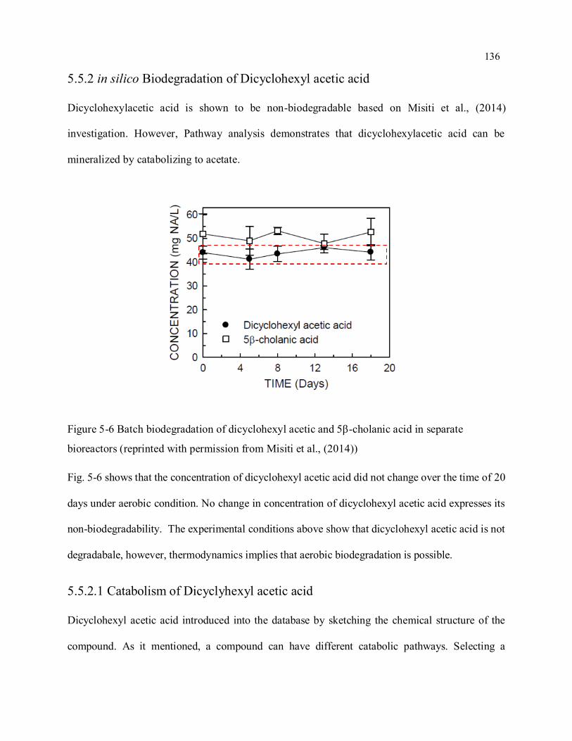
136
5.5.2 in silico Biodegradation of Dicyclohexyl acetic acid
Dicyclohexylacetic acid is shown to be non-biodegradable based on Misiti et al., (2014)
investigation. However, Pathway analysis demonstrates that dicyclohexylacetic acid can be
mineralized by catabolizing to acetate.
Figure 5-6 Batch biodegradation of dicyclohexyl acetic and 5β-cholanic acid in separate
bioreactors (reprinted with permission from Misiti et al., (2014))
Fig. 5-6 shows that the concentration of dicyclohexyl acetic acid did not change over the time of 20
days under aerobic condition. No change in concentration of dicyclohexyl acetic acid expresses its
non-biodegradability. The experimental conditions above show that dicyclohexyl acetic acid is not
degradabale, however, thermodynamics implies that aerobic biodegradation is possible.
5.5.2.1 Catabolism of Dicyclyhexyl acetic acid
Dicyclohexyl acetic acid introduced into the database by sketching the chemical structure of the
compound. As it mentioned, a compound can have different catabolic pathways. Selecting a
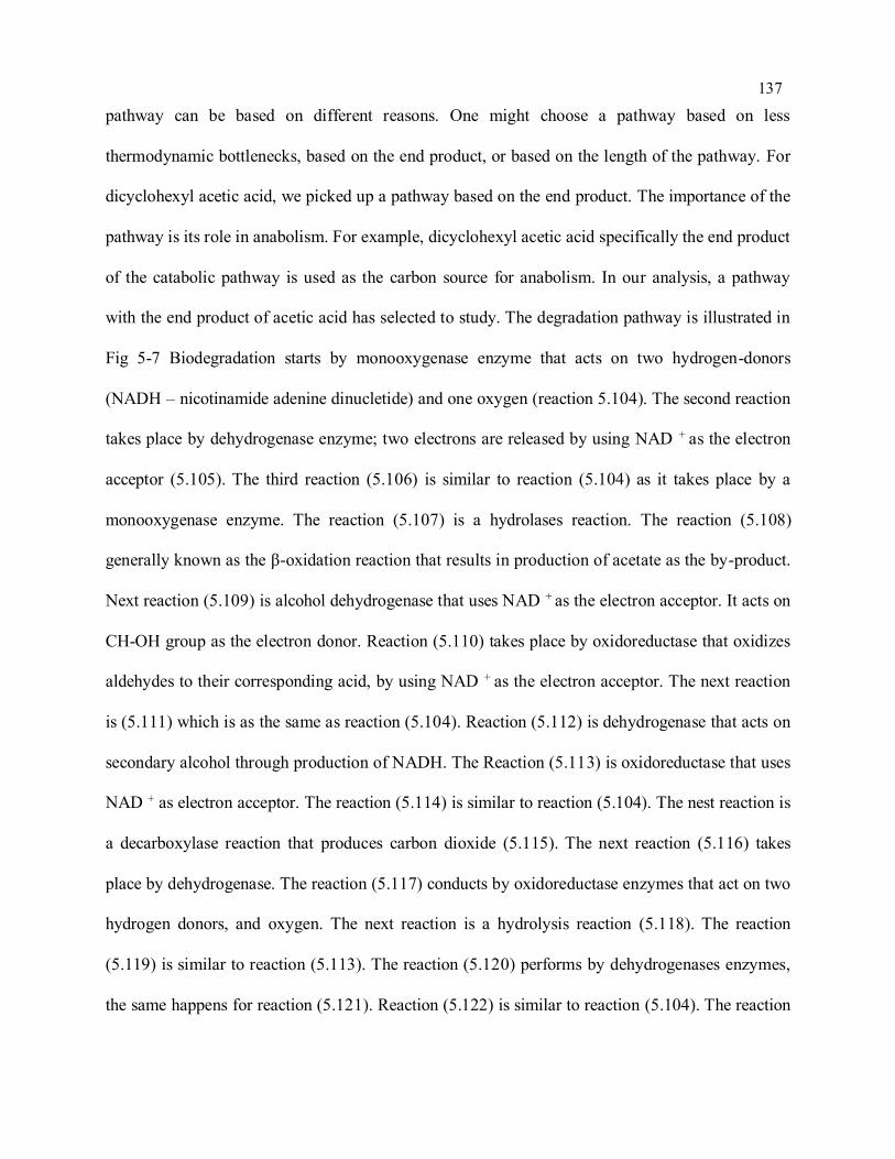
137
pathway can be based on different reasons. One might choose a pathway based on less
thermodynamic bottlenecks, based on the end product, or based on the length of the pathway. For
dicyclohexyl acetic acid, we picked up a pathway based on the end product. The importance of the
pathway is its role in anabolism. For example, dicyclohexyl acetic acid specifically the end product
of the catabolic pathway is used as the carbon source for anabolism. In our analysis, a pathway
with the end product of acetic acid has selected to study. The degradation pathway is illustrated in
Fig 5-7 Biodegradation starts by monooxygenase enzyme that acts on two hydrogen-donors
(NADH – nicotinamide adenine dinucletide) and one oxygen (reaction 5.104). The second reaction
takes place by dehydrogenase enzyme; two electrons are released by using NAD + as the electron
acceptor (5.105). The third reaction (5.106) is similar to reaction (5.104) as it takes place by a
monooxygenase enzyme. The reaction (5.107) is a hydrolases reaction. The reaction (5.108)
generally known as the β-oxidation reaction that results in production of acetate as the by-product.
Next reaction (5.109) is alcohol dehydrogenase that uses NAD + as the electron acceptor. It acts on
CH-OH group as the electron donor. Reaction (5.110) takes place by oxidoreductase that oxidizes
aldehydes to their corresponding acid, by using NAD + as the electron acceptor. The next reaction
is (5.111) which is as the same as reaction (5.104). Reaction (5.112) is dehydrogenase that acts on
secondary alcohol through production of NADH. The Reaction (5.113) is oxidoreductase that uses
NAD + as electron acceptor. The reaction (5.114) is similar to reaction (5.104). The nest reaction is
a decarboxylase reaction that produces carbon dioxide (5.115). The next reaction (5.116) takes
place by dehydrogenase. The reaction (5.117) conducts by oxidoreductase enzymes that act on two
hydrogen donors, and oxygen. The next reaction is a hydrolysis reaction (5.118). The reaction
(5.119) is similar to reaction (5.113). The reaction (5.120) performs by dehydrogenases enzymes,
the same happens for reaction (5.121). Reaction (5.122) is similar to reaction (5.104). The reaction
138
(5.123) conducts by dehydrogenase by using NAD + as electron acceptor. The reaction (5.124) is
oxidoreductase that acts on single molecular oxygen. Reaction (5.125) and reaction (5.104) is the
same again. Reaction (5.126) occurs by dehydrogenases. The next reaction (5.127) and reaction
(5.125) are the same. The reactions (5.128) and (5.129) are decarboxylases reaction that produces
CO2. And the last reaction (5.130) produces two acetic acid by using NADH as the source of
hydrogen.
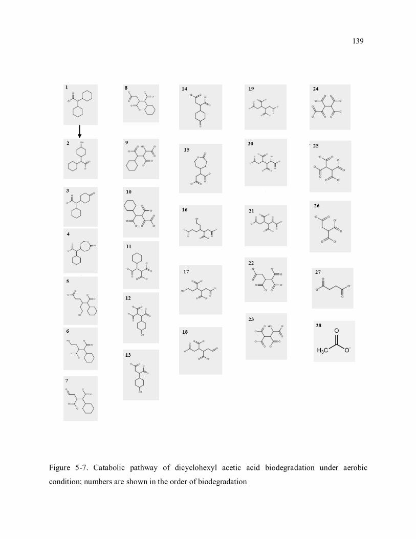
139
Figure 5-7. Catabolic pathway of dicyclohexyl acetic acid biodegradation under aerobic
condition; numbers are shown in the order of biodegradation
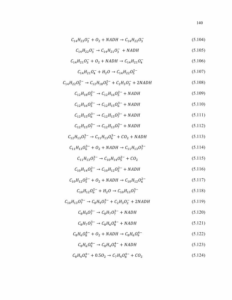
140
𝐶14𝐻23𝑂2− + 𝑂2 + 𝑁𝐴𝐷𝐻 → 𝐶14𝐻22𝑂3
− (5.104)
𝐶14𝐻22𝑂3− → 𝐶14𝐻21𝑂3
− + 𝑁𝐴𝐷𝐻 (5.105)
𝐶14𝐻21𝑂3− + 𝑂2 + 𝑁𝐴𝐷𝐻 → 𝐶14𝐻21𝑂4
− (5.106)
𝐶14𝐻21𝑂4− + 𝐻2𝑂 → 𝐶14𝐻22𝑂5
2− (5.107)
𝐶14𝐻22𝑂52− → 𝐶12𝐻18𝑂5
2− + 𝐶2𝐻3𝑂2− + 2𝑁𝐴𝐷𝐻 (5.108)
𝐶12𝐻18𝑂52− → 𝐶12𝐻16𝑂5
2− + 𝑁𝐴𝐷𝐻 (5.109)
𝐶12𝐻16𝑂52− → 𝐶12𝐻15𝑂6
3− + 𝑁𝐴𝐷𝐻 (5.110)
𝐶12𝐻15𝑂63− → 𝐶12𝐻15𝑂7
3− + 𝑁𝐴𝐷𝐻 (5.111)
𝐶12𝐻15𝑂73− → 𝐶12𝐻13𝑂7
3− + 𝑁𝐴𝐷𝐻 (5.112)
𝐶12𝐻13𝑂73− → 𝐶11𝐻13𝑂6
3− + 𝐶𝑂2 + 𝑁𝐴𝐷𝐻 (5.113)
𝐶11𝐻13𝑂63− + 𝑂2 + 𝑁𝐴𝐷𝐻 → 𝐶11𝐻13𝑂7
3− (5.114)
𝐶11𝐻13𝑂73− → 𝐶10𝐻14𝑂5
2− + 𝐶𝑂2 (5.115)
𝐶10𝐻14𝑂52− → 𝐶10𝐻12𝑂5
2− + 𝑁𝐴𝐷𝐻 (5.116)
𝐶10𝐻12𝑂52− + 𝑂2 + 𝑁𝐴𝐷𝐻 → 𝐶10𝐻12𝑂6
2− (5.117)
𝐶10𝐻12𝑂62− + 𝐻2𝑂 → 𝐶10𝐻13𝑂7
3− (5.118)
𝐶10𝐻13𝑂73− → 𝐶8𝐻9𝑂7
3− + 𝐶2𝐻3𝑂2− + 2𝑁𝐴𝐷𝐻 (5.119)
𝐶8𝐻9𝑂73− → 𝐶8𝐻7𝑂7
3− + 𝑁𝐴𝐷𝐻 (5.120)
𝐶8𝐻7𝑂73− → 𝐶8𝐻6𝑂8
4− + 𝑁𝐴𝐷𝐻 (5.121)
𝐶8𝐻6𝑂84− + 𝑂2 + 𝑁𝐴𝐷𝐻 → 𝐶8𝐻6𝑂9
4− (5.122)
𝐶8𝐻6𝑂94− → 𝐶8𝐻4𝑂9
4− + 𝑁𝐴𝐷𝐻 (5.123)
𝐶8𝐻4𝑂94− + 0.5𝑂2 → 𝐶7𝐻4𝑂8
4− + 𝐶𝑂2 (5.124)
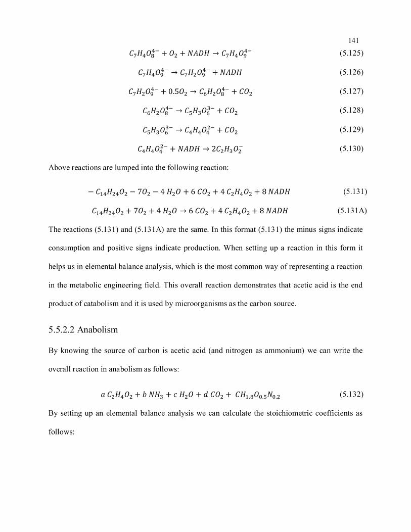
141
𝐶7𝐻4𝑂84− + 𝑂2 + 𝑁𝐴𝐷𝐻 → 𝐶7𝐻4𝑂9
4− (5.125)
𝐶7𝐻4𝑂94− → 𝐶7𝐻2𝑂9
4− + 𝑁𝐴𝐷𝐻 (5.126)
𝐶7𝐻2𝑂94− + 0.5𝑂2 → 𝐶6𝐻2𝑂8
4− + 𝐶𝑂2 (5.127)
𝐶6𝐻2𝑂84− → 𝐶5𝐻3𝑂6
3− + 𝐶𝑂2 (5.128)
𝐶5𝐻3𝑂63− → 𝐶4𝐻4𝑂4
2− + 𝐶𝑂2 (5.129)
𝐶4𝐻4𝑂42− + 𝑁𝐴𝐷𝐻 → 2𝐶2𝐻3𝑂2
− (5.130)
Above reactions are lumped into the following reaction:
− 𝐶14𝐻24𝑂2 − 7𝑂2 − 4 𝐻2𝑂 + 6 𝐶𝑂2 + 4 𝐶2𝐻4𝑂2 + 8 𝑁𝐴𝐷𝐻 (5.131)
𝐶14𝐻24𝑂2 + 7𝑂2 + 4 𝐻2𝑂 → 6 𝐶𝑂2 + 4 𝐶2𝐻4𝑂2 + 8 𝑁𝐴𝐷𝐻 (5.131A)
The reactions (5.131) and (5.131A) are the same. In this format (5.131) the minus signs indicate
consumption and positive signs indicate production. When setting up a reaction in this form it
helps us in elemental balance analysis, which is the most common way of representing a reaction
in the metabolic engineering field. This overall reaction demonstrates that acetic acid is the end
product of catabolism and it is used by microorganisms as the carbon source.
5.5.2.2 Anabolism
By knowing the source of carbon is acetic acid (and nitrogen as ammonium) we can write the
overall reaction in anabolism as follows:
𝑎 𝐶2𝐻4𝑂2 + 𝑏 𝑁𝐻3 + 𝑐 𝐻2𝑂 + 𝑑 𝐶𝑂2 + 𝐶𝐻1.8𝑂0.5𝑁0.2 (5.132)
By setting up an elemental balance analysis we can calculate the stoichiometric coefficients as
follows:

142
(
2 0 0 1 14 3 2 0 1.82 0 1 2 0.50 1 0 0 0.28 0 0 0 4.2)
∙
(
𝑎𝑏𝑐𝑑1)
= 0
(5.133)
By multiplying the above matrix we have:
𝐶 − 𝑏𝑎𝑙𝑎𝑛𝑐𝑒: 2𝑎 + 𝑑 + 1 = 0 (5.134)
𝐻 − 𝑏𝑎𝑙𝑎𝑛𝑐𝑒: 4𝑎 + 3𝑏 + 2𝐶 + 1.8 = 0 (5.135)
𝑂 − 𝑏𝑎𝑙𝑎𝑛𝑐𝑒: 2𝑎 + 𝑐 + 2𝑑 + 0.5 = 0 (5.136)
𝑁 − 𝑏𝑎𝑙𝑎𝑛𝑐𝑒: 𝑏 + 0.2 = 0 (5.137)
𝛾 − 𝑏𝑎𝑙𝑎𝑛𝑐𝑒: 8 𝑎 + 4.2 = 0 (5.138)
Solving the above equation results in:
(
𝑎𝑏𝑐𝑑1)
=
(
−0.525−0.20.450.051 )
(5.139)
Now we have the anabolic reaction based on the production of 1 C-mol biomass using acetic acid
as a carbon source.
By recalling Eq (5.98):
1
𝑌𝐺𝑋𝑚𝑎𝑥 = 200 + 18(6 − 𝐶)1.8 + 𝑒𝑥𝑝[|3.8 − 𝛾|0.32 × (3.6 + 0.4𝐶)] [
𝑘𝐽
𝐶 − 𝑚𝑜𝑙𝑒𝐶𝑥]
Based on this equation we can calculate the Gibbs energy of dissipation for growth of 1
C-mole biomass on acetate. Acetate has 2 carbon with degree of reduction of 4 mole
electron per C-mole atom.
1
𝑌𝐺𝑋𝑚𝑎𝑥 = 200 + 18(6 − 2)1.8 + 𝑒𝑥𝑝[|3.8 − 4|0.32 × (3.6 + 0.4 × 2)] [
𝑘𝐽
𝐶 − 𝑚𝑜𝑙𝑒𝐶𝑥
]
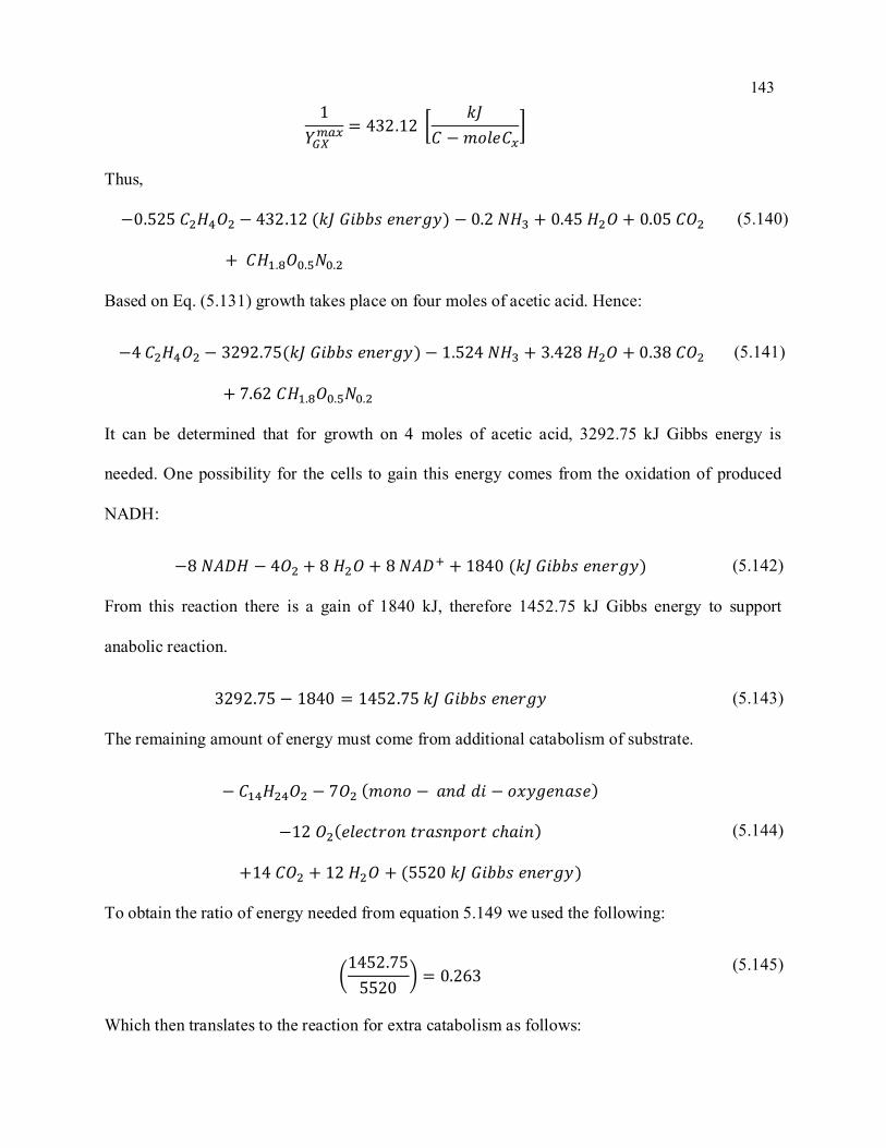
143
1
𝑌𝐺𝑋𝑚𝑎𝑥 = 432.12 [
𝑘𝐽
𝐶 − 𝑚𝑜𝑙𝑒𝐶𝑥]
Thus,
−0.525 𝐶2𝐻4𝑂2 − 432.12 (𝑘𝐽 𝐺𝑖𝑏𝑏𝑠 𝑒𝑛𝑒𝑟𝑔𝑦) − 0.2 𝑁𝐻3 + 0.45 𝐻2𝑂 + 0.05 𝐶𝑂2
+ 𝐶𝐻1.8𝑂0.5𝑁0.2
(5.140)
Based on Eq. (5.131) growth takes place on four moles of acetic acid. Hence:
−4 𝐶2𝐻4𝑂2 − 3292.75(𝑘𝐽 𝐺𝑖𝑏𝑏𝑠 𝑒𝑛𝑒𝑟𝑔𝑦) − 1.524 𝑁𝐻3 + 3.428 𝐻2𝑂 + 0.38 𝐶𝑂2
+ 7.62 𝐶𝐻1.8𝑂0.5𝑁0.2
(5.141)
It can be determined that for growth on 4 moles of acetic acid, 3292.75 kJ Gibbs energy is
needed. One possibility for the cells to gain this energy comes from the oxidation of produced
NADH:
−8 𝑁𝐴𝐷𝐻 − 4𝑂2 + 8 𝐻2𝑂 + 8 𝑁𝐴𝐷+ + 1840 (𝑘𝐽 𝐺𝑖𝑏𝑏𝑠 𝑒𝑛𝑒𝑟𝑔𝑦) (5.142)
From this reaction there is a gain of 1840 kJ, therefore 1452.75 kJ Gibbs energy to support
anabolic reaction.
3292.75 − 1840 = 1452.75 𝑘𝐽 𝐺𝑖𝑏𝑏𝑠 𝑒𝑛𝑒𝑟𝑔𝑦 (5.143)
The remaining amount of energy must come from additional catabolism of substrate.
− 𝐶14𝐻24𝑂2 − 7𝑂2 (𝑚𝑜𝑛𝑜 − 𝑎𝑛𝑑 𝑑𝑖 − 𝑜𝑥𝑦𝑔𝑒𝑛𝑎𝑠𝑒)
−12 𝑂2(𝑒𝑙𝑒𝑐𝑡𝑟𝑜𝑛 𝑡𝑟𝑎𝑠𝑛𝑝𝑜𝑟𝑡 𝑐ℎ𝑎𝑖𝑛)
+14 𝐶𝑂2 + 12 𝐻2𝑂 + (5520 𝑘𝐽 𝐺𝑖𝑏𝑏𝑠 𝑒𝑛𝑒𝑟𝑔𝑦)
(5.144)
To obtain the ratio of energy needed from equation 5.149 we used the following:
(1452.75
5520) = 0.263
(5.145)
Which then translates to the reaction for extra catabolism as follows:
144
− 0.263 𝐶14𝐻24𝑂2 − 1.841 𝑂2(𝑚𝑜𝑛𝑜 − 𝑜𝑥) − 3.156 𝑂2(𝐸𝑇𝐶) + 3.682 𝐶𝑂2
+ 3.156 𝐻2𝑂 + 1452.75 𝑘𝐽 𝐺𝑖𝑏𝑏𝑠 𝑒𝑛𝑒𝑟𝑔𝑦
(5.146)
To get the overall growth (biodegradation) reaction we need to sum up reactions (5.131),
(5.141),(5.142), and (5.146):
−1.263 𝐶14𝐻24𝑂2 − 15.997 𝑂2 − 1.524 𝑁𝐻3 + 7.62 𝐶𝐻1.8𝑂0.5𝑁0.2 + 10.584 𝐻2𝑂
+ 10.062 𝐶𝑂2
(5.147)
5.8.4. Calculation of yield of substrate to biomass
To calculate the yield of substrate to biomass using equation 5.147 we have:
𝑌𝑠𝑥 =7.62
1.263 × 14= 0.431
𝐶 − 𝑚𝑜𝑙 𝑏𝑖𝑜𝑚𝑎𝑠𝑠
𝐶 − 𝑚𝑜𝑙 𝑠𝑢𝑏𝑠𝑡𝑟𝑎𝑡𝑒= 0.663
𝑔 𝑜𝑟𝑔𝑎𝑛𝑖𝑐 𝑑𝑟𝑦 𝑤𝑒𝑖𝑔ℎ𝑡
𝑔 𝑠𝑢𝑏𝑠𝑡𝑟𝑎𝑡𝑒
(5.148)
The accuracy in the prediction of yield of substrate to biomass by the proposed approach, has a
relative error of 13%.
145
Figure 5-8 Comparison of measured and predicted yield of substrate to biomass; ( ) shows the
fermentative growth system and ( ) shows the aerobic growth system; taken from (reprinted with
permission from Heijnen et. al, (1992))
5.5.2.1.1 Calculation of µmax
In production of energy through electron transport chain ~ 460 kJ Gibbs energy is produced per
mole of electron. This number comes from following reaction:
𝑂2 + 𝑁𝐴𝐷𝐻 → 2𝑁𝐴𝐷+ + 2𝐻2𝑂 ; ∆𝐺 = −460 𝑘𝐽/𝑚𝑜𝑙
Therefore, 115 kJ energy is produced per mole of catabolized electron (1 mole of oxygen
contains 4 mole of electron). With this the maximum specific growth rate of biomass can be
calculated.
By recalling following equation:
𝑞𝐺𝑚𝑎𝑥 = 3 ∙ (
∆𝐺𝑐𝑎𝑡
𝑛) 𝑒𝑥𝑝 [−
69000
𝑅(1
𝑇−
1
298)] [
𝑘𝐽
𝐶 − 𝑚𝑜𝑙𝑒 𝐶𝑥. ℎ]
At T=298 K:
𝑞𝐺𝑚𝑎𝑥 = 3 × 115 = 345 [
𝑘𝐽
𝐶 − 𝑚𝑜𝑙𝑒 𝐶𝑥. ℎ]
Thus,
µ𝑚𝑎𝑥 = (𝑞𝐺
𝑚𝑎𝑥 − 𝑚𝐺
1𝑌𝐺𝑋
𝑚𝑎𝑥
) = (345 − 4.5
432) = 0.788 ℎ−1
5.5.2.3 Needed Substrate for Maintenance
By using equation (5.97), the energy required for maintenance can be calculated.
146
𝑚𝐺 = 4.5 𝑒𝑥𝑝 [−69000
𝑅(1
𝑇−
1
298)] [
𝑘𝐽
𝐶 − 𝑚𝑜𝑙𝑒𝐶𝑥. ℎ]
At T=298 K we have:
𝑚𝐺 = 4.5 [𝑘𝐽
𝐶 − 𝑚𝑜𝑙𝑒𝐶𝑥. ℎ]
Hence, due to equation (5.96)
𝑚𝑠 =4.5
5520= 8.15 × 10⁻⁴
𝑚𝑜𝑙 𝐶𝑠
𝐶 − 𝑚𝑜𝑙 𝐶𝑥 ∙ ℎ
Maintenance substrate for other compounds:
𝑚𝑂2=
4.5 × (7 + 12)
5520= 0.0154
𝑚𝑜𝑙 𝑂2
𝐶 − 𝑚𝑜𝑙 𝐶𝑥 ∙ ℎ
𝑚𝐶𝑂2=
4.5 × 14
5520= 0.0114
𝑚𝑜𝑙 𝐶𝑂2
𝐶 − 𝑚𝑜𝑙 𝐶𝑥 ∙ ℎ
𝑚𝐻2𝑂 =4.5 × 12
5890= 0.0098
𝑚𝑜𝑙 𝐻2𝑂
𝐶 − 𝑚𝑜𝑙 𝐶𝑥 ∙ ℎ
Above calculations demonstrate the substrate needed (oxygen and substrate) and produced
(carbon dioxide and water) in maintenance. As maintenance is defined as the needed substrate at
zero growth rate and at zero growth rate, no biomass is produced. Therefore, a nitrogen source is
not needed here.
Since the yields and maintenance substrate have been determined, a Herbert-Pirt equation can be
written for each compound.
𝑞𝑠 = (1.263
7.62)𝜇 + 8.15 × 10⁻⁴ [
𝑚𝑜𝑙 𝐶𝑠
𝐶−𝑚𝑜𝑙 𝐶𝑥∙ℎ]
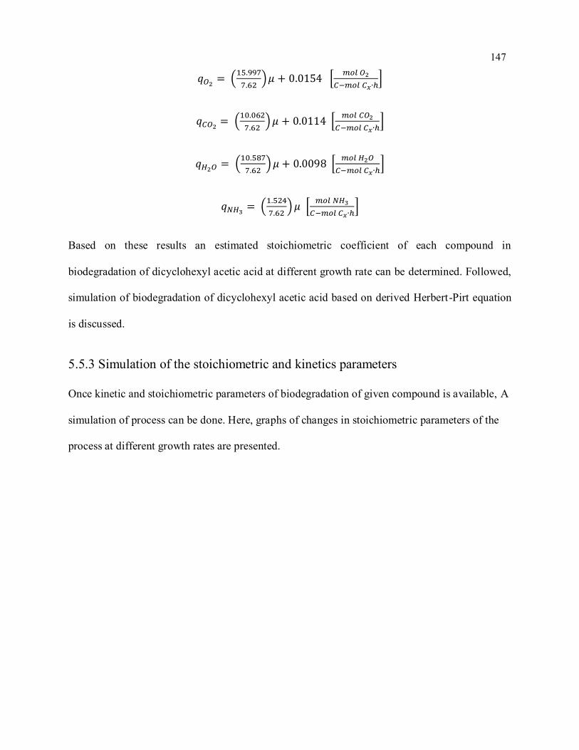
147
𝑞𝑂2= (
15.997
7.62)𝜇 + 0.0154 [
𝑚𝑜𝑙 𝑂2
𝐶−𝑚𝑜𝑙 𝐶𝑥∙ℎ]
𝑞𝐶𝑂2= (
10.062
7.62)𝜇 + 0.0114 [
𝑚𝑜𝑙 𝐶𝑂2
𝐶−𝑚𝑜𝑙 𝐶𝑥∙ℎ]
𝑞𝐻2𝑂= (
10.587
7.62)𝜇 + 0.0098 [
𝑚𝑜𝑙 𝐻2𝑂
𝐶−𝑚𝑜𝑙 𝐶𝑥∙ℎ]
𝑞𝑁𝐻3= (
1.524
7.62)𝜇 [
𝑚𝑜𝑙 𝑁𝐻3
𝐶−𝑚𝑜𝑙 𝐶𝑥∙ℎ]
Based on these results an estimated stoichiometric coefficient of each compound in
biodegradation of dicyclohexyl acetic acid at different growth rate can be determined. Followed,
simulation of biodegradation of dicyclohexyl acetic acid based on derived Herbert-Pirt equation
is discussed.
5.5.3 Simulation of the stoichiometric and kinetics parameters
Once kinetic and stoichiometric parameters of biodegradation of given compound is available, A
simulation of process can be done. Here, graphs of changes in stoichiometric parameters of the
process at different growth rates are presented.
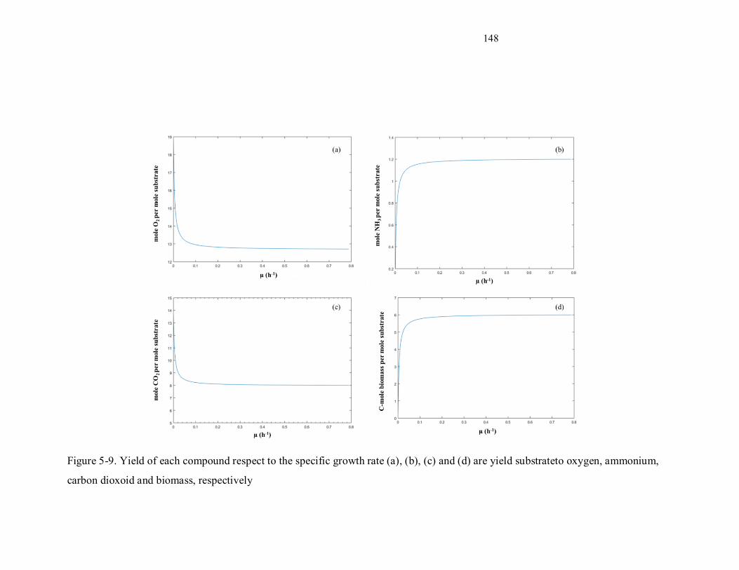
148
Figure 5-9. Yield of each compound respect to the specific growth rate (a), (b), (c) and (d) are yield substrateto oxygen, ammonium,
carbon dioxoid and biomass, respectively
149
In graph 5-9(a), y-axis shows the mole of oxygen consumed per unit of biomass specific
consumption rate. This axis represents the amount of required oxygen per unit of consumed
substrate. The x-axis represents the biomass specific growth rate. For instance, environmental
engineering would want a fast and efficient treatment. Therefore, with the faster a qs (rate of
consumption of substrate per unit of biomass), the more efficient systems produced. And graph
(a) in Fig. 5.9 illustrates that when µ is more than 0.2 h-1, 13 moles of oxygen are needed for
consumption of one mole of substrate; however, at specific growth rate ~0.02, this ratio is 15. At
the first glance, the difference between 15 mole and 13 moles of oxygen is not very big.
However, it should be realized that this small difference can be very significant in long runs and
huge volumes. The same explanation can be done on other parameters i.e. CO2 and NH3.
Accordingly, relation which are provided by thermodynamics can help us in prediction and
optimization of the process. Following section discusses the in silico biodegradation of
dicyclohexyl acetic acid and comparison of results with experimental data.
5.5.3.1 Estimation of Substrate Affinity
In general there is no thermodynamic approach for prediction of substrate affinity. However, one
of the logical approaches for estimation of substrate affinity for low soluble compounds is using
their solubility (Colin Ratledge, 2006; Smolke, 2009). It means that solubility can be directly
considered as the substrate affinity. Therefore, solubility of dicyclohlohexyl acetic acid estimated
as 0.724 mM at 25 degree of C and pH=7 (Hou et al., 2004b; Shoghi et al., 2013).
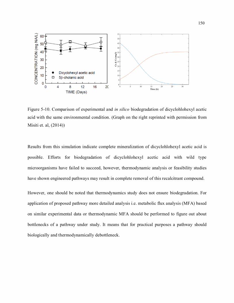
150
Figure 5-10. Comparison of experimental and in silico biodegradation of dicyclohlohexyl acetic
acid with the same environmental condition. (Graph on the right reprinted with permission from
Misiti et. al, (2014))
Results from this simulation indicate complete mineralization of dicyclohlohexyl acetic acid is
possible. Efforts for biodegradation of dicyclohlohexyl acetic acid with wild type
microorganisms have failed to succeed, however, thermodynamic analysis or feasibility studies
have shown engineered pathways may result in complete removal of this recalcitrant compound.
However, one should be noted that thermodynamics study does not ensure biodegradation. For
application of proposed pathway more detailed analysis i.e. metabolic flux analysis (MFA) based
on similar experimental data or thermodynamic MFA should be performed to figure out about
bottlenecks of a pathway under study. It means that for practical purposes a pathway should
biologically and thermodynamically debottleneck.
151
5.6 Conclusion
In the world of NAs treatment, there has been a successful advancement in molecular, chemical,
and kinetic analysis for either model NAs, commercially produced or OSPW associated NAs. As
well, kinetic and stoichiometric parameters for bioremediation of NAs under different
physiological condition has been determined. Partial biodegradability of commercial, tailings
associated and various model NAs have been proved.
Computational tools to predict novel biodegradation pathways of target compounds allow us to
investigate the power of microorganisms to consume pollutants as their source of carbon and
energy (Darvas, Gómez et al., 2007; Greene et al., 1999; Henry et al., 2006; Jaworska et al.,
2002; Klopman et al., 1994; Rodrigo et al., 2008). Therefore, these computational tools i.e. UM-
BBD gives us the opportunity to explore the possible metabolic pathways for biodegradation of
model NAs.
Results from in silico investigation of NAs biodegradation illustrate that by implementing
genetic and metabolic engineering tools, it is possible to design a cell factory to degrade NAs.
For bioremediation purposes, design of catabolic pathways is the main interest (Finley et al.,
2009a; Finley et al., 2009b; Hatzimanikatis et al., 2005). Through a thermodynamic favorable
catabolic pathway with non-toxic (end-) products, complete mineralization of a pollutant is
achievable (Alexander, 1999; Finley et al., 2009b; de la Peña Mattozzi et al., 2006; Walker and
Keasling, 2002). However, thermodynamic favourability can be manipulated through genetic
manipulation (i.e. expression of specific gene for production of higher protein respect wild type)
(Henry et al., 2006; Henry et al., 2007; Smolke, 2009).
152
In general, due to author’s knowledge, systems biology approaches have not been conducted for
the case of NAs biodegradation. Successful investigation of systems biology aspects of NAs
bioremediation may result in development of more capable microbial cultures for consumption
of NAs. Moreover, establishment of microbial consortium is another advantages of systems and
synthetic biology field. Synergies among microbes can be seen as an asset in improving the
mineralization of organic pollutants. These interactions may result in detoxification of some
metabolites (Gilbert et al., 2003; Mukherji and van Oudenaarden, 2009).
153
5.7 References
Alberty RA. 1998. Calculation of standard transformed formation properties of biochemical
reactants and standard apparent reduction potentials of half reactions. Arch. Biochem.
Biophys. 358:25–39.
Alexander M. 1985. Biodegradation of organic chemicals. Environ. Sci. Technol. 19:106–111.
Alexander M. 1999. Biodegradation and Bioremediation. Gulf Professional Publishing 453 p.
Beeftink HH, Heijden RTJM, Heijnen JJ. 1990. Maintenance requirements: energy supply from
simultaneous endogenous respiration and substrate consumption. FEMS Microbiol. Lett.
73:203–209.
Boopathy R. 2000. Factors limiting bioremediation technologies. Bioresour. Technol. 74:63–67.
Chauhan G, Stein M, Seidel-Morgenstern A, Pant KK, Nigam KDP. 2015. The thermodynamics
and biodegradability of chelating agents upon metal extraction. Chem. Eng. Sci. 137:768–
785.
Colin Ratledge BK. 2006. Basic Biotechnology. Cambridge University Press 666 p.
Cueto-Rojas HF, van Maris AJA, Wahl SA, Heijnen JJ. 2015. Thermodynamics-based design of
microbial cell factories for anaerobic product formation. Trends Biotechnol. 33:534–46.
Darvas F. MetabolExpert, an expert system for predicting metabolism of substances. QSAR
Environ. Toxicol.
Demirel Y. 2014a. Nonequilibrium Thermodynamics. Nonequilibrium Thermodyn. Elsevier 1-74
p.
Demirel Y. 2014b. Nonequilibrium Thermodynamics. Nonequilibrium Thermodyn. Elsevier 752-
758 p.
Dolfing J, Larter SR, Head IM. 2008. Thermodynamic constraints on methanogenic crude oil
biodegradation. ISME J. 2:442–52.
Dolfing J, Xu A, Gray ND, Larter SR, Head IM. 2009. The thermodynamic landscape of
154
methanogenic PAH degradation. Microb. Biotechnol. 2:566–74.
Dong F, Nemati M. 2016. Anoxic biodegradation of a surrogate naphthenic acid coupled to
reduction of nitrite. Biochem. Eng. J.
Dua M, Singh A, Sethunathan N, Johri AK. 2002. Biotechnology and bioremediation: successes
and limitations. Appl. Microbiol. Biotechnol. 59:143–52.
Ellis LBM, Roe D, Wackett LP. 2006. The University of Minnesota Biocatalysis/Biodegradation
Database: the first decade. Nucleic acids Res. 34.
Erickson LE, Davis LC, Narayanan M. 1995. Bioenergetics and bioremediation of contaminated
soil. Thermochim. Acta 250:353–358.
Feist AM, Henry CS, Reed JL, Krummenacker M, Joyce AR, Karp PD, Broadbelt LJ,
Hatzimanikatis V, Palsson BØ. 2007. A genome-scale metabolic reconstruction for
Escherichia coli K-12 MG1655 that accounts for 1260 ORFs and thermodynamic
information. Mol. Syst. Biol. 3:121.
Finley SD, Broadbelt LJ, Hatzimanikatis V. 2009a. Thermodynamic analysis of biodegradation
pathways. Biotechnol. Bioeng. 103:532–41.
Finley SD, Broadbelt LJ, Hatzimanikatis V. 2009b. Computational framework for predictive
biodegradation. Biotechnol. Bioeng. 104:1086–97.
Finley SD, Broadbelt LJ, Hatzimanikatis V. 2010. In silico feasibility of novel biodegradation
pathways for 1,2,4-trichlorobenzene. BMC Syst. Biol. 4:7.
Flickinger MC. 2009. Encyclopedia of Industrial Biotechnology. Hoboken, NJ, USA: John
Wiley & Sons, Inc.
Gavrilescu M, Demnerová K, Aamand J, Agathos S, Fava F. 2015. Emerging pollutants in the
environment: present and future challenges in biomonitoring, ecological risks and
bioremediation. N. Biotechnol. 32:147–56.
Gilbert ES, Walker AW, Keasling JD. 2003. A constructed microbial consortium for
biodegradation of the organophosphorus insecticide parathion. Appl. Microbiol. Biotechnol.
155
61:77–81.
Gómez MJ, Pazos F, Guijarro FJ, de Lorenzo V, Valencia A. 2007. The environmental fate of
organic pollutants through the global microbial metabolism. Mol. Syst. Biol. 3:114.
Greene N, Judson PN, Langowski JJ, Marchant CA. 1999. Knowledge-based expert systems for
toxicity and metabolism prediction: DEREK, StAR and METEOR. SAR QSAR Environ.
Res. 10:299–314.
Groot SR De, Mazur P. 1962. Non-Equilibrium Thermodynamics. Courier Corporation 528 p.
Hatzimanikatis V, Li C, Ionita JA, Henry CS, Jankowski MD, Broadbelt LJ. 2005. Exploring the
diversity of complex metabolic networks. Bioinformatics 21:1603–9.
Heijnen JJ. 2010. Impact of thermodynamic principles in systems biology. Adv. Biochem. Eng.
Biotechnol. 121:139–62.
Heijnen JJ. 1991. A new thermodynamically based correlation of chemotrophic biomass yields.
Antonie Van Leeuwenhoek 60:235–256.
Heijnen JJ, Van Dijken JP. 1992. In search of thermodynamic description of biomass yields for
the chemotrophic growth of microorganisms. Biotechnol. Bioeng.
Henry CS, Broadbelt LJ, Hatzimanikatis V. 2007. Thermodynamics-based metabolic flux
analysis. Biophys. J. 92:1792–805.
Henry CS, Jankowski MD, Broadbelt LJ, Hatzimanikatis V. 2006. Genome-scale
thermodynamic analysis of Escherichia coli metabolism. Biophys. J. 90:1453–61.
Hoijnen JJ, van Loosdrecht MC, Tijhuis L. 1992. A black box mathematical model to calculate
auto- and heterotrophic biomass yields based on Gibbs energy dissipation. Biotechnol.
Bioeng. 40:1139–54.
Hou BK, Ellis LBM, Wackett LP. 2004a. Encoding microbial metabolic logic: predicting
biodegradation. J. Ind. Microbiol. Biotechnol. 31:261–72.
Hou BK, Wackett LP, Ellis LBM. 2003. Microbial pathway prediction: a functional group
156
approach. J. Chem. Inf. Comput. Sci. 43:1051–7.
Hou TJ, Xia K, Zhang W, Xu XJ. 2004b. ADME evaluation in drug discovery. 4. Prediction of
aqueous solubility based on atom contribution approach. J. Chem. Inf. Comput. Sci. 44:266–
75.
Huang J, Nemati M, Hill G, Headley J. 2012. Batch and continuous biodegradation of three
model naphthenic acids in a circulating packed-bed bioreactor. J. Hazard. Mater. 201-
202:132–40.
Jankowski MD, Henry CS, Broadbelt LJ, Hatzimanikatis V. 2008. Group contribution method
for thermodynamic analysis of complex metabolic networks. Biophys. J. 95:1487–99.
Jaworska J, Dimitrov S, Nikolova N, Mekenyan O. 2002. Probabilistic assessment of
biodegradability based on metabolic pathways: catabol system. SAR QSAR Environ. Res.
13:307–323.
Klopman G, Dimayuga M, Talafous J. 1994. META. 1. A program for the evaluation of
metabolic transformation of chemicals. J. Chem. Inf. Comput. Sci. 34:1320–1325.
Kovar K, Chaloupka V, Egli T. 2002. A Threshold Substrate Concentration Is Required to
Initiate the Degradation of 3-Phenylpropionic Acid in Escherichia coli. Acta Biotechnol.
22:285–298.
Kovarova-Kovar K, Egli T. 1998. Growth Kinetics of Suspended Microbial Cells: From Single-
Substrate-Controlled Growth to Mixed-Substrate Kinetics. Microbiol. Mol. Biol. Rev.
62:646–666.
Kristiansen CRB. 1999, eds. Basic biotechnology. Cambridge University Press
de la Peña Mattozzi M, Tehara SK, Hong T, Keasling JD. 2006. Mineralization of paraoxon and
its use as a sole C and P source by a rationally designed catabolic pathway in Pseudomonas
putida. Appl. Environ. Microbiol. 72:6699–706.
Lehninger AL, Nelson DL, Cox MM. 2005. Lehninger Principles of Biochemistry. W. H.
Freeman 1119 p.
157
Mavrovouniotis ML. 1990. Group contributions for estimating standard gibbs energies of
formation of biochemical compounds in aqueous solution. Biotechnol. Bioeng. 36:1070–82.
Mavrovouniotis ML. 1991. Estimation of standard Gibbs energy changes of biotransformations.
J. Biol. Chem. 266:14440–14445.
Meckenstock RU, Elsner M, Griebler C, Lueders T, Stumpp C, Aamand J, Agathos SN,
Albrechtsen H-J, Bastiaens L, Bjerg PL, Boon N, Dejonghe W, Huang WE, Schmidt SI,
Smolders E, Sørensen SR, Springael D, van Breukelen BM. 2015. Biodegradation:
Updating the concepts of control for microbial cleanup in contaminated aquifers. Environ.
Sci. Technol. 49:7073–81.
Misiti T, Tezel U, Pavlostathis S. 2014. Effect of alkyl side chain location and cyclicity on the
aerobic biotransformation of naphthenic acids. Environ. Sci. ….
Mukherji S, van Oudenaarden A. 2009. Synthetic biology: understanding biological design from
synthetic circuits. Nat. Rev. Genet. 10:859–71.
Oller I, Polo-López I, Miralles-Cuevas S, Fernández-Ibáñez P, Malato S. 2014. Advanced
Technologies for Emerging Contaminants Removal in Urban Wastewater:1–25.
Onsager L. 1931. Reciprocal Relations in Irreversible Processes. I. Phys. Rev. 37:405–426.
Paslawski JC, Headley J V, Hill GA, Nemati M. 2009. Biodegradation kinetics of trans-4-
methyl-1-cyclohexane carboxylic acid. Biodegradation 20:125–33.
Paul D, Pandey G, Pandey J, Jain RK. 2005. Accessing microbial diversity for bioremediation
and environmental restoration. Trends Biotechnol. 23:135–42.
Petrie B, Barden R, Kasprzyk-Hordern B. 2014. A review on emerging contaminants in
wastewaters and the environment: Current knowledge, understudied areas and
recommendations for future monitoring. Water Res. 72:3–27.
Pirt SJ. 1965. The Maintenance Energy of Bacteria in Growing Cultures. Proc. R. Soc. B Biol.
Sci. 163:224–231.
Prigogine I. 1968. Introduction to thermodynamics of irreversible processes. Interscience
158
Publishers 147 p.
Reddy KR, DeLaune RD. 2008. Biogeochemistry of Wetlands: Science and Applications. CRC
Press 800 p.
Rittmann B, McCarty P. 2012. Environmental biotechnology: principles and applications.
Rodrigo G, Carrera J, Prather KJ, Jaramillo A. 2008. DESHARKY: automatic design of
metabolic pathways for optimal cell growth. Bioinformatics 24:2554–6.
Roels JA. 1983. Energetics and kinetics in biotechnology.
Russell JB, Cook GM. 1995. Energetics of bacterial growth: balance of anabolic and catabolic
reactions. Microbiol. Rev. 59:48–62.
S. Roy Caplan AE. 1983. Bioenergetics and Linear Nonequilibrium Thermodynamics. Harvard
Univ. Press. http://www.hup.harvard.edu/catalog.php?isbn=9780674732063.
Shoghi E, Fuguet E, Bosch E, Ràfols C. 2013. Solubility-pH profiles of some acidic, basic and
amphoteric drugs. Eur. J. Pharm. Sci. 48:291–300.
Smith JM, Ness HC Van, Abbott MM. 2001. Introduction to Chemical Engineering
Thermodynamics. McGraw-Hill 789 p.
Smolke C. 2009. The Metabolic Pathway Engineering Handbook: Fundamentals. CRC Press 678
p.
Stephanopoulos G, Aristidou AA, Nielsen J. 1998. Metabolic Engineering: Principles and
Methodologies. Academic Press 725 p.
von Stockar U, Maskow T, Liu J, Marison IW, Patiño R. 2006. Thermodynamics of microbial
growth and metabolism: an analysis of the current situation. J. Biotechnol. 121:517–33.
Tchobanoglous G, Burton FL, Stensel HD, Eddy M&. 2003. Wastewater Engineering: Treatment
and Reuse. McGraw-Hill Education 1819 p.
Tijhuis L, Van Loosdrecht MCM, Heijnen JJ. 1993. A thermodynamically based correlation for
maintenance Gibbs energy requirements in aerobic and anaerobic chemotrophic growth.
159
Biotechnol. Bioeng. 42:509–519.
Urs von Stockar LAM van der W. 2013. Biothermodynamics: The Role of Thermodynamics in
Biochemical Engineering. https://www.crcpress.com/Biothermodynamics-The-Role-of-
Thermodynamics-in-Biochemical-Engineering/Stockar-van-der-Wielen/9781466582163.
Van Loosdrecht M, Henze M. 1999. Maintenance, endogeneous respiration, lysis, decay and
predation. Water Sci. Technol. 39:107–117.
Wackett LP, Ellis LB. 1999. Predicting biodegradation. Environ. Microbiol. 1:119–24.
Walker AW, Keasling JD. 2002. Metabolic engineering of Pseudomonas putida for the
utilization of parathion as a carbon and energy source. Biotechnol. Bioeng. 78:715–21.
Welch GR. 1985. Some problems in the usage of gibbs free energy in biochemistry. J. Theor.
Biol. 114:433–446.
Westerhoff H V., Dam K van. 1987. Thermodynamics and control of biological free-energy
transduction. Elsevier 568 p.
Westerhoff HV. 1983. Mosaic Non-equilibrium Thermodynamics and (the Control Of)
Biological Free- Energy Transduction. Drukkerij Gerja 368 p.
Wylen GJ Van, Sonntag RE, Borgnakke C. 1994. Fundamentals of Classical Thermodynamics,
Volume 1. Wiley 852 p.
Zotin AI. 1990. Thermodynamic Bases of Biological Processes: Physiological Reactions and
Adaptations. Walter de Gruyter 293 p.
160
CHAPTER 6. CONCLUSIONS AND RECOMMENDATIONS
6.1 Thesis Overview
Devastating effects of oil sands process affected water (OSPW) and tailings ponds on the
environment were the main driving forces of this research. There is no doubt OSPW in tailings
ponds needs to be remediated. Efforts are still striving to achieve an efficient, and practical
strategy to remediate OSPW. To accomplish this goal, many research teams are focusing on
varying methods to determine a proven practical treatment strategy.
6.2 Summary of Findings
In 2013, inactivated sodium persulfate and potassium permanganate used for the first time for
removal of naphthenic acids (NAs) in OSPW. Results showed the reactivity of persulfate and
permanganate toward NAs. A challenge the obtained results from chemical oxidation
experiments has is a lack of stoichiometric information in the process. Stoichiometric parameters
are among the main parameters that have critical role in design, application and optimization of
the oxidation process. In chapter 3 of this thesis, a stoichiometrically-based design was
performed to estimate the required amount of persulfate for treatment purposes. The main factor
in the proposed design was the amount of available electrons in the wastewater. The amount of
available electrons was determined by a chemical oxygen demand measurement. Then, for the
determination of required oxidant, the degree of reduction of oxidant was considered to calculate
the theoretical oxidant dosage. Results showed the model successfully demonstrated outcomes
which resulted in degradation of NAs. Summaries of findings described below:
Complete understanding of detailed chemistry behind NAs oxidation is not necessarily
needed for its application.
161
More than 90% degradation in the NAs concentration achieved in 28 days with less than
20% of needed persulfate from the previously published data.
Case study for treatment of MLSB OSPW demonstrates we can save 110,000 tonnes of
persulfate, which equates to a 290 million dollars saving.
Due to huge volume of OSPW in tailings ponds, when oxidation with a chemical oxidant
is of interest, results from lab scale experiments need to be gone through optimzation
processes.
Understanding the stoichiometry of oxidation reactions can significantly improve the
remediation process based on chemical oxidation.
After successful degradation of NAs by persulfate, the idea of coupling chemical and biological
oxidation was considered as the next step. In chapter 4 of this work the effect of persulfate on
ability of microorganisms in removal of NAs is discussed. Results are summarized below:
Stress test affected the maximum concentration of biomass. By increasing the
concentration of oxidant, the maximum concentration of Pseudomonas sp. is decreased.
At the dosage of 2000 mg/L, no growth was observed.
In spite the high oxidative stress, the bacteria could still consume Merichem NAs as the
sole source of carbon and energy.
Quantitative physiology applied to compare the effect of oxidative stress on
biodegradation. Biomass, specific growth rate, yield of substrate to biomass, and biomass
specific substrate consumption rate, were not significantly different among different
series.
The bacteria that are stressed with 1000 mg/L of sodium persulfate had a 15.5 hr lag time,
while other series had almost the same lag time.

162
Chemical oxidation with sodium persulfate can couple with biological oxidation.
In chapter 6 of this work, thermodynamics of NAs biodegradation was investigated for the first
time as fundamental step in this field. Power of thermodynamics in prediction of unknown
163
1.Broda E. 1976. Two kinds of lithotrophs missing in nature. Z. Allg. Mikrobiol. 17:491–493.
2.Strous M, Fuerst JA, Kramer EH, Logemann S, Muyzer G, van de Pas-Schoonen KT, Webb R,
Kuenen JG, Jetten MS. 1999. Missing lithotroph identified as new planctomycete. Nature
400:446–9.
processes has been proved before. For instance, in 1976 Broda published a paper entitle of “two
lithotrophs are missing in nature” (Broda, 1976)1. He predicted based on thermodynamics
calculation that ammonia can be anaerobically oxidized to nitrogen gas by using nitrite as the
electron acceptor by microorganisms. Years later, in 1999, Strous and coworkers published a
paper in nature entitle “missing lithotrophs identified as new planctomycetes” (Strous et al.,
1999)2. This was one of the examples among so many other findings based on a thermodynamic
understanding. Some important points of thermodynamics founding are:
Thermodynamics feasibility study should be conducted as the first step in attempt to
biodegrade recalcitrant compounds.
Experimental results suggest a non-biodegradability of dicyclohexyl acetic acid,
however, thermodynamics predict the complete mineralization of this compound under
aerobic condition
Catabolic pathways are the most important process in biodegradability of model NAs.
Improvement of a strain of a wild type microorganism for degradation of a model NAs
would result in enhancement of biodegradation of other model NAs. This is because
almost all of classical NAs have same Gibbs energy of formation (~ 107 kJ per electron
mole).
Predicted stoichiometric and kinetics parameters i.e. yield of substrate to biomass,
amount if needed nitrogen source, amount of needed oxygen, based on thermodynamics
can be used in design and optimization of biodegradation processes.
164
6.3 Significance of the Research
In the chapters of this thesis, have tried to address the removal of NAs with different
perspectives. For chemical oxidation (chapter 3), a simple model based on the available electrons
in OSPW has been proposed to determine the needed amount of oxidant. Results have shown the
model’s results predict effective concentrations. This model has attempted to estimate the desired
parameter (amount of required oxidant) with less available information. The model would be a
good tool at industrial level. In chapter 4, design parameters that are required in design of a
bioprocess is determined. Findings represent feasible coupling of chemical and biological
oxidation by using sodium persulfate as the oxidant. Theoretical analyses based on the
thermodynamics behind biodegradation of NAs can build up a new road with the expectation of
biodegradation of previously believed non-biodegradable NAs.
6.4 Recommendations for Future Work
1. Simultaneous application of persulfate and biological oxidation
It is interesting to see the simultaneous chemical oxidation (by sodium persulfate) and biological
oxidation of NAs. Chemical oxidation and biological oxidation have different rate in degradation
of NAs. Differenet parameters can affect each rate. Therefore, rate-based modelling can be used
with the aim of optimization of the process.
2. Thermodynamics metabolic flux analysis (TMFA)
Application of systems biology tools like TMFA can greatly impact the world of NAs
biodegradation. These tools allow one to investigate the design of engineered microorganisms
with more detailed perspective. By TMFA optimized flux of interacellular (and also extracelluar)
metabolites can be determined. Results can help further improvmnets of microorganisms through
gene manipulation for production of higher/lower determined enzymes.
165
3. Estimation of the threshold concentration of naphthenic acids for microorganisms
One of the gaps in the world of NAs biodegradation is lack of the knowledge of threshold
concentration. This gap might arise a question that the remaining concentration of NAs in aged
oil sands tailings ponds is below the threshold concentration for microorganisms, therefore, they
cannot consume it. An experimental approach is proposed here to estimate the threshold
concentration of NAs.
For this purpose, experiments to calculate steady state biodegradation rate at different
concentration of NAs (highest possible to lowest possible) need to be conducted. Then, the
biodegradation rate should be plotted versus its corresponding concentration. By extrapolating
the hyperbolic curve to zero rate, where the curve meets x-axis, we can determine the threshold
concentration. However, this threshold does not tell us the biological threshold. This threshold
might have chemical and physical origin, for instance, it can be mass transfer limitation
(diffusion) or dissolution limitation. To overcome this issue, the second part should be
performed.
At this step, the same experiments need to be conducted but with highest rate of mixing. Higher
mixing rate would eliminate transport phenomena limitations and dissolution limitation. Again,
as the same as first part, biodegradation rate is plotted against concentration of substrate. Where,
the hyperbolic curve, meets the x-axis which means that at the extrapolated concentration the
biodegradation rate is zero. This point is a good approximate of biological threshold. However,
determination of a threshold concentration for a specific substrate is very tedious. The proposed
idea, however, can be used as a good first approximate.
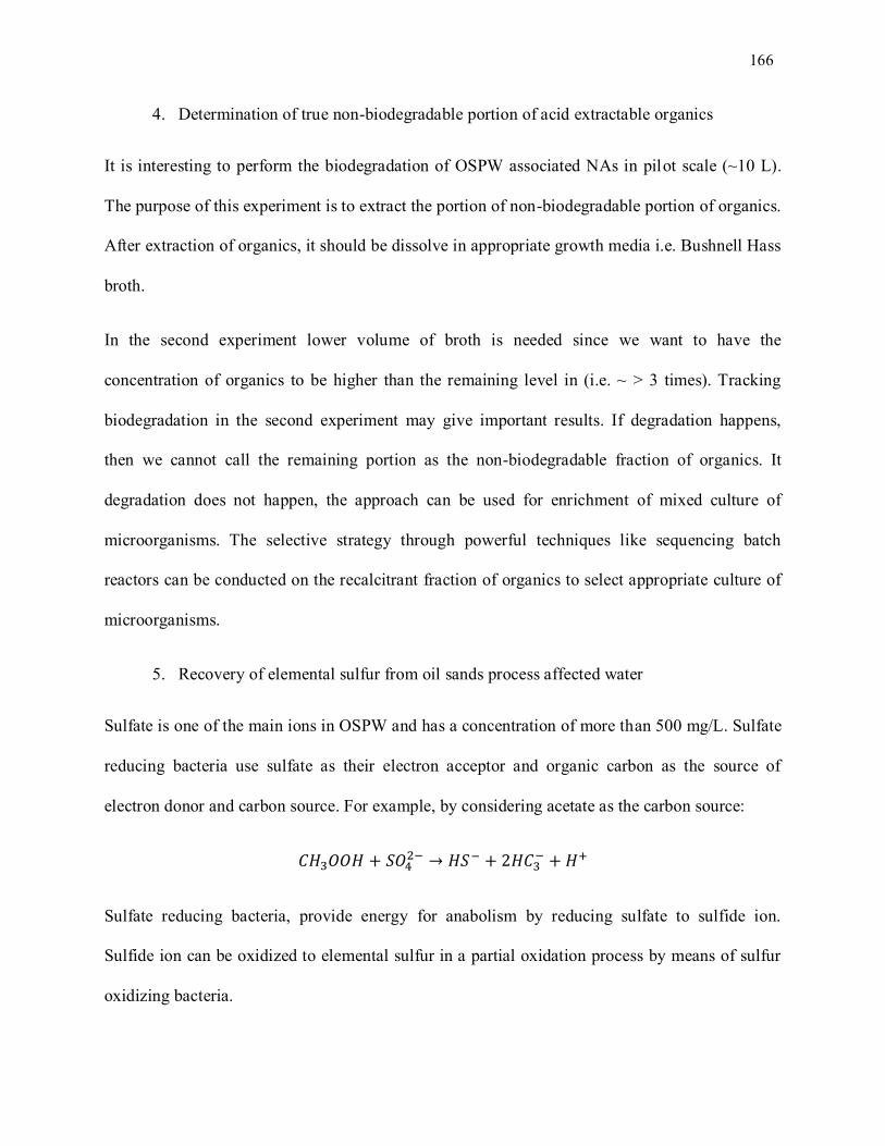
166
4. Determination of true non-biodegradable portion of acid extractable organics
It is interesting to perform the biodegradation of OSPW associated NAs in pilot scale (~10 L).
The purpose of this experiment is to extract the portion of non-biodegradable portion of organics.
After extraction of organics, it should be dissolve in appropriate growth media i.e. Bushnell Hass
broth.
In the second experiment lower volume of broth is needed since we want to have the
concentration of organics to be higher than the remaining level in (i.e. ~ > 3 times). Tracking
biodegradation in the second experiment may give important results. If degradation happens,
then we cannot call the remaining portion as the non-biodegradable fraction of organics. It
degradation does not happen, the approach can be used for enrichment of mixed culture of
microorganisms. The selective strategy through powerful techniques like sequencing batch
reactors can be conducted on the recalcitrant fraction of organics to select appropriate culture of
microorganisms.
5. Recovery of elemental sulfur from oil sands process affected water
Sulfate is one of the main ions in OSPW and has a concentration of more than 500 mg/L. Sulfate
reducing bacteria use sulfate as their electron acceptor and organic carbon as the source of
electron donor and carbon source. For example, by considering acetate as the carbon source:
𝐶𝐻3𝑂𝑂𝐻 + 𝑆𝑂42− → 𝐻𝑆− + 2𝐻𝐶3
− + 𝐻+
Sulfate reducing bacteria, provide energy for anabolism by reducing sulfate to sulfide ion.
Sulfide ion can be oxidized to elemental sulfur in a partial oxidation process by means of sulfur
oxidizing bacteria.
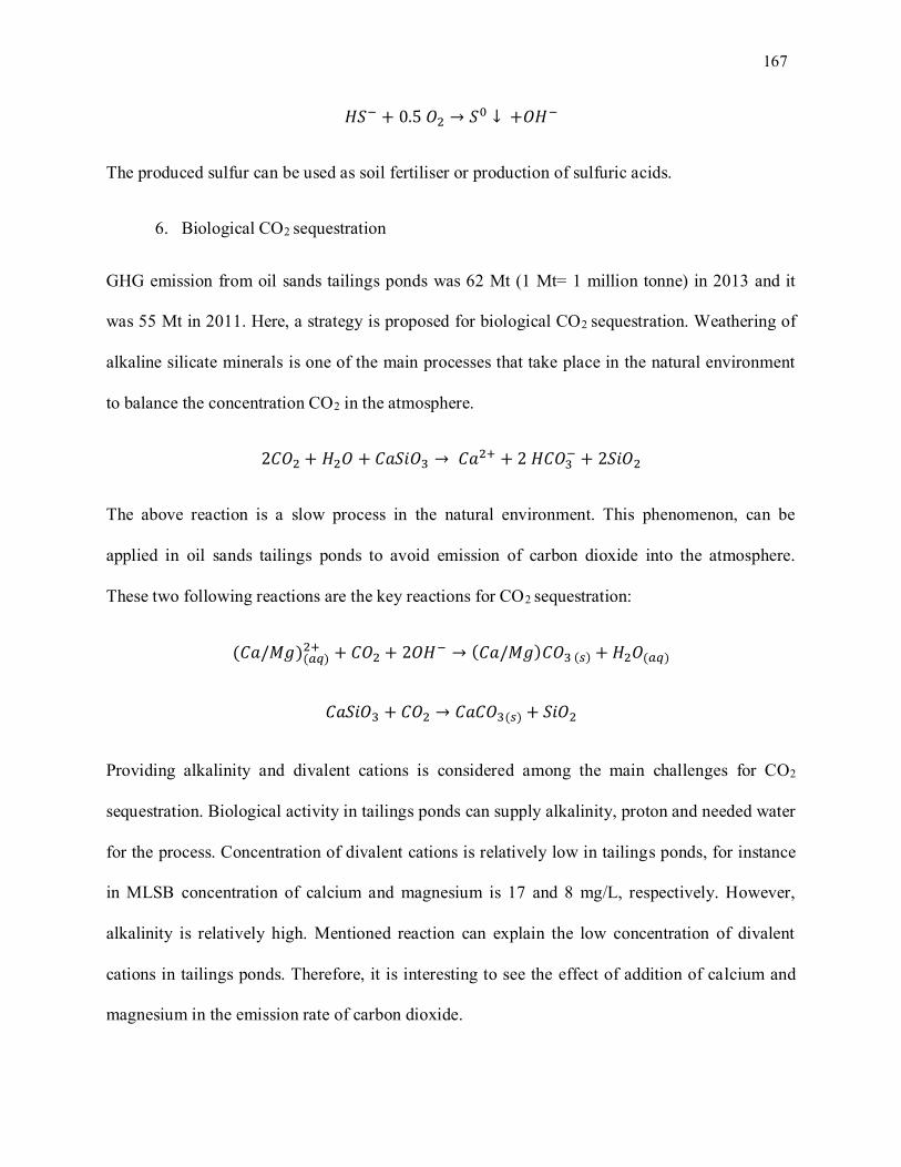
167
𝐻𝑆− + 0.5 𝑂2 → 𝑆0 ↓ +𝑂𝐻−
The produced sulfur can be used as soil fertiliser or production of sulfuric acids.
6. Biological CO2 sequestration
GHG emission from oil sands tailings ponds was 62 Mt (1 Mt= 1 million tonne) in 2013 and it
was 55 Mt in 2011. Here, a strategy is proposed for biological CO2 sequestration. Weathering of
alkaline silicate minerals is one of the main processes that take place in the natural environment
to balance the concentration CO2 in the atmosphere.
2𝐶𝑂2 + 𝐻2𝑂 + 𝐶𝑎𝑆𝑖𝑂3 → 𝐶𝑎2+ + 2 𝐻𝐶𝑂3− + 2𝑆𝑖𝑂2
The above reaction is a slow process in the natural environment. This phenomenon, can be
applied in oil sands tailings ponds to avoid emission of carbon dioxide into the atmosphere.
These two following reactions are the key reactions for CO2 sequestration:
(𝐶𝑎/𝑀𝑔)(𝑎𝑞)2+ + 𝐶𝑂2 + 2𝑂𝐻− → (𝐶𝑎/𝑀𝑔)𝐶𝑂3 (𝑠) + 𝐻2𝑂(𝑎𝑞)
𝐶𝑎𝑆𝑖𝑂3 + 𝐶𝑂2 → 𝐶𝑎𝐶𝑂3(𝑠) + 𝑆𝑖𝑂2
Providing alkalinity and divalent cations is considered among the main challenges for CO2
sequestration. Biological activity in tailings ponds can supply alkalinity, proton and needed water
for the process. Concentration of divalent cations is relatively low in tailings ponds, for instance
in MLSB concentration of calcium and magnesium is 17 and 8 mg/L, respectively. However,
alkalinity is relatively high. Mentioned reaction can explain the low concentration of divalent
cations in tailings ponds. Therefore, it is interesting to see the effect of addition of calcium and
magnesium in the emission rate of carbon dioxide.
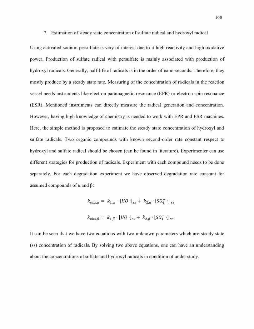
168
7. Estimation of steady state concentration of sulfate radical and hydroxyl radical
Using activated sodium persulfate is very of interest due to it high reactivity and high oxidative
power. Production of sulfate radical with persulfate is mainly associated with production of
hydroxyl radicals. Generally, half-life of radicals is in the order of nano-seconds. Therefore, they
mostly produce by a steady state rate. Measuring of the concentration of radicals in the reaction
vessel needs instruments like electron paramagnetic resonance (EPR) or electron spin resonance
(ESR). Mentioned instruments can directly measure the radical generation and concentration.
However, having high knowledge of chemistry is needed to work with EPR and ESR machines.
Here, the simple method is proposed to estimate the steady state concentration of hydroxyl and
sulfate radicals. Two organic compounds with known second-order rate constant respect to
hydroxyl and sulfate radical should be chosen (can be found in literature). Experimenter can use
different strategies for production of radicals. Experiment with each compound needs to be done
separately. For each degradation experiment we have observed degradation rate constant for
assumed compounds of α and β:
𝑘𝑜𝑏𝑠,𝛼 = 𝑘1,α ∙ [𝐻𝑂 ∙]𝑠𝑠 + 𝑘2,𝛼 ∙ [𝑆𝑂4− ∙] 𝑠𝑠
𝑘𝑜𝑏𝑠,𝛽 = 𝑘1,𝛽 ∙ [𝐻𝑂 ∙]𝑠𝑠 + 𝑘2,𝛽 ∙ [𝑆𝑂4− ∙] 𝑠𝑠
It can be seen that we have two equations with two unknown parameters which are steady state
(ss) concentration of radicals. By solving two above equations, one can have an understanding
about the concentrations of sulfate and hydroxyl radicals in condition of under study.
169
BIBLIOGRAPHY
Abolfazlzadehdoshanbehbazari M, Birks SJ, Moncur MC, Ulrich AC. 2013. Fate and transport
of oil sand process-affected water into the underlying clay till: a field study. J. Contam.
Hydrol. 151:83–92.
Alaton IA, Dogruel S, Baykal E, Gerone G. 2004. Combined chemical and biological oxidation
of penicillin formulation effluent. J. Environ. Manage. 73:155–63.
Alberty RA. 1998. Calculation of standard transformed formation properties of biochemical
reactants and standard apparent reduction potentials of half reactions. Arch. Biochem.
Biophys. 358:25–39.
Alexander M. 1985. Biodegradation of organic chemicals. Environ. Sci. Technol. 19:106–111.
Alexander M. 1999. Biodegradation and Bioremediation. Gulf Professional Publishing 453 p.
Allen EW. 2008a. Process water treatment in Canada’s oil sands industry: I. Target pollutants
and treatment objectives. J. Environ. Eng. Sci. 7:123–138.
Allen EW. 2008b. Process water treatment in Canada’s oil sands industry: II. A review of
emerging technologies. J. Environ. Eng. Sci. 7:499–524.
Andersson DI, Hughes D. 2014. Microbiological effects of sublethal levels of antibiotics. Nat.
Rev. Microbiol. 12:465–78.
Andreozzi R. 1999. Advanced oxidation processes (AOP) for water purification and recovery.
Catal. Today 53:51–59.
Andrews JM. 2001. Determination of minimum inhibitory concentrations. J. Antimicrob.
Chemother. 48:5–16.
Anfruns A, Gabarró J, Gonzalez-Olmos R, Puig S, Balaguer MD, Colprim J. 2013. Coupling
anammox and advanced oxidation-based technologies for mature landfill leachate treatment.
J. Hazard. Mater. 258-259:27–34.
Bailey JE. 1986. Biochemical Engineering Fundamentals. McGraw-Hill 984 p.
Bard AJ, Faulkner LR. 2000. Electrochemical Methods: Fundamentals and Applications, 2nd
Edition. John Wiley & Sons 856 p.
170
Beeftink HH, Heijden RTJM, Heijnen JJ. 1990. Maintenance requirements: energy supply from
simultaneous endogenous respiration and substrate consumption. FEMS Microbiol. Lett.
73:203–209.
Blakley ER, Papish B. 1982. The metabolism of cyclohexanecarboxylic acid and 3-
cyclohexenecarboxylic acid by Pseudomonas putida. Can. J. Microbiol. 28:1324–9.
Blakley ER. 1974. The microbial degradation of cyclohexanecarboxylic acid: a pathway
involving aromatization to form p hydroxybenzoic acid. Can. J. Microbiol.
Boender LGM, de Hulster EAF, van Maris AJA, Daran-Lapujade PAS, Pronk JT. 2009.
Quantitative physiology of Saccharomyces cerevisiae at near-zero specific growth rates.
Appl. Environ. Microbiol. 75:5607–14.
Boopathy R. 2000. Factors limiting bioremediation technologies. Bioresour. Technol. 74:63–67.
Boudens R, Reid T, VanMensel D, Prakasan M R S, Ciborowski JJH, Weisener CG. 2016. Bio-
physicochemical effects of gamma irradiation treatment for naphthenic acids in oil sands
fluid fine tailings. Sci. Total Environ. 539:114–24.
Broda E. 1976. Two kinds of lithotrophs missing in nature. Z. Allg. Mikrobiol. 17:491–493.
Brown LD, Pérez-Estrada L, Wang N, El-Din MG, Martin JW, Fedorak PM, Ulrich AC. 2013.
Indigenous microbes survive in situ ozonation improving biodegradation of dissolved
organic matter in aged oil sands process-affected waters. Chemosphere 93:2748–55.
Brown LD, Ulrich AC. 2015. Oil sands naphthenic acids: a review of properties, measurement,
and treatment. Chemosphere 127:276–90.
Cabiscol E, Tamarit J, Ros J. 2000. Oxidative stress in bacteria and protein damage by reactive
oxygen species. Int. Microbiol.
Camel V, Bermond A. 1998. The use of ozone and associated oxidation processes in drinking
water treatment. Water Res. 32:3208–3222.
Cassidy D, Northup A, Hampton D. 2009. The effect of three chemical oxidants on subsequent
biodegradation of 2,4-dinitrotoluene (DNT) in batch slurry reactors. J. Chem. Technol.
Biotechnol. 84:820–826.
Chakravarti R, Patrick BN, Barney M, Kusinski G, Devine TM. 2013. Toward the Mechanism of
171
Corrosion in Crude Oil: A Study Using Vibrational Spectroscopic Techniques at Elevated
Temperatures. Energy & Fuels 27:7905–7914.
Chapman JS. 2003. Disinfectant resistance mechanisms, cross-resistance, and co-resistance. Int.
Biodeterior. Biodegradation 51:271–276.
Chauhan G, Stein M, Seidel-Morgenstern A, Pant KK, Nigam KDP. 2015. The thermodynamics
and biodegradability of chelating agents upon metal extraction. Chem. Eng. Sci. 137:768–
785.
Chen K-F, Chang Y-C, Chiou W-T. 2015. Remediation of diesel-contaminated soil using in situ
chemical oxidation (ISCO) and the effects of common oxidants on the indigenous microbial
community: a comparison study. J. Chem. Technol. Biotechnol.:n/a–n/a.
Christopher Grant Weisener JJHC. 2013. Gamma Radiation Apparatus for Remediation of
Organic Compounds in Waste Slurries.
Chung C-H, Fen S-Y, Yu S-C, Wong H-C. 2015. Influence of oxyR on Growth, Biofilm
Formation, and Mobility of Vibrio parahaemolyticus. Appl. Environ. Microbiol. 82:788–96.
Clark DS, Blanch HW. 1995. Biochemical Engineering, Second Edition. CRC Press 702 p.
Clemente JS, Fedorak PM. 2005. A review of the occurrence, analyses, toxicity, and
biodegradation of naphthenic acids. Chemosphere 60:585–600.
Clemente JS, Prasad NG., MacKinnon MD, Fedorak PM. 2003. A statistical comparison of
naphthenic acids characterized by gas chromatography–mass spectrometry. Chemosphere
50:1265–1274.
Clothier LN, Gieg LM. 2016. Anaerobic biodegradation of surrogate naphthenic acids. Water
Res. 90:156–66.
Colin Ratledge BK. 2006. Basic Biotechnology. Cambridge University Press 666 p.
Cornish-Bowden A. 2013. Fundamentals of Enzyme Kinetics. John Wiley & Sons 510 p.
Cruz M-J, De Vooght V, Muñoz X, Hoet PHM, Morell F, Nemery B, Vanoirbeek JAJ. 2009.
Assessment of the sensitization potential of persulfate salts used for bleaching hair. Contact
Dermatitis 60:85–90.
Cueto-Rojas HF, van Maris AJA, Wahl SA, Heijnen JJ. 2015. Thermodynamics-based design of
172
microbial cell factories for anaerobic product formation. Trends Biotechnol. 33:534–46.
Darvas F. MetabolExpert, an expert system for predicting metabolism of substances. QSAR
Environ. Toxicol.
de la Peña Mattozzi M, Tehara SK, Hong T, Keasling JD. 2006. Mineralization of paraoxon and
its use as a sole C and P source by a rationally designed catabolic pathway in Pseudomonas
putida. Appl. Environ. Microbiol. 72:6699–706.
Del Rio LF, Hadwin AKM, Pinto LJ, MacKinnon MD, Moore MM. 2006. Degradation of
naphthenic acids by sediment micro-organisms. J. Appl. Microbiol. 101:1049–61.
Demeter MA, Lemire JA, Yue G, Ceri H, Turner RJ. 2015. Culturing oil sands microbes as
mixed species communities enhances ex situ model naphthenic acid degradation. Front.
Microbiol. 6:936.
Demirel Y. 2014b. Nonequilibrium Thermodynamics. Nonequilibrium Thermodyn. Elsevier 752-
758 p.
Demple B. 1991. Regulation of bacterial oxidative stress genes. Annu. Rev. Genet. 25:315–37.
Derungs WA. 1956. Naphthenic Acid Corrosion —An Old Enemy Of the Petroleum Industry ★.
Corrosion 12:41–46.
Dolfing J, Larter SR, Head IM. 2008. Thermodynamic constraints on methanogenic crude oil
biodegradation. ISME J. 2:442–52.
Dolfing J, Xu A, Gray ND, Larter SR, Head IM. 2009. The thermodynamic landscape of
methanogenic PAH degradation. Microb. Biotechnol. 2:566–74.
Dong F, Nemati M. 2016. Anoxic biodegradation of a surrogate naphthenic acid coupled to
reduction of nitrite. Biochem. Eng. J.
Doran PM. 1995. Bioprocess Engineering Principles. Bioprocess Eng. Princ. Elsevier 426-439 p.
Drzewicz P, Perez-Estrada L, Alpatova A, Martin JW, Gamal El-Din M. 2012. Impact of
peroxydisulfate in the presence of zero valent iron on the oxidation of cyclohexanoic acid
and naphthenic acids from oil sands process-affected water. Environ. Sci. Technol.
46:8984–91.
173
Dua M, Singh A, Sethunathan N, Johri AK. 2002. Biotechnology and bioremediation: successes
and limitations. Appl. Microbiol. Biotechnol. 59:143–52.
Ellis LBM, Roe D, Wackett LP. 2006. The University of Minnesota Biocatalysis/Biodegradation
Database: the first decade. Nucleic acids Res. 34.
Ellis TG, Barbeau DS, Smets BF, Grady CPL. 1996. Respirometric technique for determination
of extant kinetic parameters describing biodegradation. Water Environ. Res. 68:917–926.
Elmén J, Pan W, Leung SY, Magyarosy A, Keasling JD. 1997. Kinetics of toluene degradation
by a nitrate-reducing bacterium isolated from a groundwater aquifer. Biotechnol. Bioeng.
55:82–90.
Erickson LE, Davis LC, Narayanan M. 1995. Bioenergetics and bioremediation of contaminated
soil. Thermochim. Acta 250:353–358.
Esteves BM, Rodrigues CSD, Boaventura RAR, Maldonado-Hódar FJ, Madeira LM. 2016.
Coupling of acrylic dyeing wastewater treatment by heterogeneous Fenton oxidation in a
continuous stirred tank reactor with biological degradation in a sequential batch reactor. J.
Environ. Manage. 166:193–203.
Farr SB, Kogoma T. 1991. Oxidative stress responses in Escherichia coli and Salmonella
typhimurium. Microbiol. Mol. Biol. Rev. 55:561–585.
Feist AM, Henry CS, Reed JL, Krummenacker M, Joyce AR, Karp PD, Broadbelt LJ,
Hatzimanikatis V, Palsson BØ. 2007. A genome-scale metabolic reconstruction for
Escherichia coli K-12 MG1655 that accounts for 1260 ORFs and thermodynamic
information. Mol. Syst. Biol. 3:121.
Finley SD, Broadbelt LJ, Hatzimanikatis V. 2009. Thermodynamic analysis of biodegradation
pathways. Biotechnol. Bioeng. 103:532–41.
Finley SD, Broadbelt LJ, Hatzimanikatis V. 2009a. Computational framework for predictive
biodegradation. Biotechnol. Bioeng. 104:1086–97.
Finley SD, Broadbelt LJ, Hatzimanikatis V. 2010. In silico feasibility of novel biodegradation
pathways for 1,2,4-trichlorobenzene. BMC Syst. Biol. 4:7.
174
Flickinger MC. 2009. Encyclopedia of Industrial Biotechnology. Hoboken, NJ, USA: John
Wiley & Sons, Inc.
Frank RA, Fischer K, Kavanagh R, Burnison BK, Arsenault G, Headley J V., Peru KM, Kraak G
Van Der, Solomon KR. 2009. Effect of Carboxylic Acid Content on the Acute Toxicity of
Oil Sands Naphthenic Acids. Environ. Sci. Technol. 43:266–271.
Frank RA, Sanderson H, Kavanagh R, Burnison BK, Headley J V, Solomon KR. 2010. Use of a
(quantitative) structure-activity relationship [(Q)SAR] model to predict the toxicity of
naphthenic acids. J. Toxicol. Environ. Health. A 73:319–29.
Gambino M, Cappitelli F. 2016. Mini-review: Biofilm responses to oxidative stress. Biofouling
32:167–78.
Garcia-Garcia E, Ge JQ, Oladiran A, Montgomery B, El-Din MG, Perez-Estrada LC, Stafford
JL, Martin JW, Belosevic M. 2011. Ozone treatment ameliorates oil sands process water
toxicity to the mammalian immune system. Water Res. 45:5849–57.
Gavrilescu M, Demnerová K, Aamand J, Agathos S, Fava F. 2015. Emerging pollutants in the
environment: present and future challenges in biomonitoring, ecological risks and
bioremediation. N. Biotechnol. 32:147–56.
Ghanizadeh G, Naseri Ara A, Esmaili D, Masoumbeigi H. 2015. Demonstration of the Enhanced
Disinfection of E. coli Water Contamination by Associated Solar Irradiation with Potassium
Persulfate. Iran. J. Public Health 44:1376–86.
Giesy JP, Anderson JC, Wiseman SB. 2010. Alberta oil sands development. Proc. Natl. Acad.
Sci. U. S. A. 107:951–2.
Gilbert ES, Walker AW, Keasling JD. 2003. A constructed microbial consortium for
biodegradation of the organophosphorus insecticide parathion. Appl. Microbiol. Biotechnol.
61:77–81.
Gómez MJ, Pazos F, Guijarro FJ, de Lorenzo V, Valencia A. 2007. The environmental fate of
organic pollutants through the global microbial metabolism. Mol. Syst. Biol. 3:114.
Government of Alberta. 2010. Tailings.
Government of Alberta. 2016. Oil sands quarterly. Open Text Web Site Management.
175
Greene N, Judson PN, Langowski JJ, Marchant CA. 1999. Knowledge-based expert systems for
toxicity and metabolism prediction: DEREK, StAR and METEOR. SAR QSAR Environ.
Res. 10:299–314.
Grewer DM, Young RF, Whittal RM, Fedorak PM. 2010. Naphthenic acids and other acid-
extractables in water samples from Alberta: what is being measured? Sci. Total Environ.
408:5997–6010.
Groot SR De, Mazur P. 1962. Non-Equilibrium Thermodynamics. Courier Corporation 528 p.
Guieysse B, Norvill ZN. 2014. Sequential chemical-biological processes for the treatment of
industrial wastewaters: review of recent progresses and critical assessment. J. Hazard.
Mater. 267:142–52.
Gunawan Y, Nemati M, Dalai A. 2014. Biodegradation of a surrogate naphthenic acid under
denitrifying conditions. Water Res. 51:11–24.
Gupta A, Rao G. 2003. A study of oxygen transfer in shake flasks using a non-invasive oxygen
sensor. Biotechnol. Bioeng. 84:351–8.
Guzel-Seydim ZB, Greene AK, Seydim AC. 2004. Use of ozone in the food industry. LWT -
Food Sci. Technol. 37:453–460.
Hack N, Reinwand C, Abbt-Braun G, Horn H, Frimmel FH. 2015. Biodegradation of phenol,
salicylic acid, benzenesulfonic acid, and iomeprol by Pseudomonas fluorescens in the
capillary fringe. J. Contam. Hydrol. 183:40–54.
Halliwell B, Gutteridge JMC. 1985. Free radicals in biology and medicine.
Hammes F, Vital M, Egli T. 2010. Critical evaluation of the volumetric “bottle effect” on
microbial batch growth. Appl. Environ. Microbiol. 76:1278–81.
Han X, Scott AC, Fedorak PM, Bataineh M, Martin JW. 2008. Influence of Molecular Structure
on the Biodegradability of Naphthenic Acids. Environ. Sci. Technol. 42:1290–1295.
Harding HP, Zhang Y, Zeng H, Novoa I, Lu PD, Calfon M, Sadri N, Yun C, Popko B, Paules R,
Stojdl DF, Bell JC, Hettmann T, Leiden JM, Ron D. 2003. An Integrated Stress Response
Regulates Amino Acid Metabolism and Resistance to Oxidative Stress. Mol. Cell 11:619–
633.
176
Hatzimanikatis V, Li C, Ionita JA, Henry CS, Jankowski MD, Broadbelt LJ. 2005. Exploring the
diversity of complex metabolic networks. Bioinformatics 21:1603–9.
He Y, Patterson S, Wang N, Hecker M, Martin JW, El-Din MG, Giesy JP, Wiseman SB. 2012.
Toxicity of untreated and ozone-treated oil sands process-affected water (OSPW) to early
life stages of the fathead minnow (Pimephales promelas). Water Res. 46:6359–68.
Headley J V, Peru KM, Barrow MP, Derrick PJ. 2007. Characterization of naphthenic acids from
athabasca oil sands using electrospray ionization: the significant influence of solvents. Anal.
Chem. 79:6222–9.
Headley J V, Peru KM, Mohamed MH, Frank RA, Martin JW, Hazewinkel RRO, Humphries D,
Gurprasad NP, Hewitt LM, Muir DCG, Lindeman D, Strub R, Young RF, Grewer DM,
Whittal RM, Fedorak PM, Birkholz DA, Hindle R, Reisdorph R, Wang X, Kasperski KL,
Hamilton C, Woudneh M, Wang G, Loescher B, Farwell A, Dixon DG, Ross M, Pereira
ADS, King E, Barrow MP, Fahlman B, Bailey J, McMartin DW, Borchers CH, Ryan CH,
Toor NS, Gillis HM, Zuin L, Bickerton G, Mcmaster M, Sverko E, Shang D, Wilson LD,
Wrona FJ. 2013. Chemical fingerprinting of naphthenic acids and oil sands process waters-
A review of analytical methods for environmental samples. J. Environ. Sci. Health. A. Tox.
Hazard. Subst. Environ. Eng. 48:1145–63.
Headley J V., McMartin DW. 2004. A review of the occurrence and fate of naphthenic acids in
aquatic environments. J. Environ. Sci. Heal. - Part A Toxic/Hazardous Subst. Environ. Eng.
Headley J V., McMartin DW. 2004. A review of the occurrence and fate of naphthenic acids in
aquatic environments. J. Environ. Sci. Heal. - Part A Toxic/Hazardous Subst. Environ. Eng.
177
Headley J V., McMartin DW. 2004. A review of the occurrence and fate of naphthenic acids in
aquatic environments. J. Environ. Sci. Heal. - Part A Toxic/Hazardous Subst. Environ. Eng.
Headley J V., McMartin DW. 2007. A Review of the Occurrence and Fate of Naphthenic Acids
in Aquatic Environments. J. Environ. Sci. Heal. Part A.
Heijnen JJ, Van Dijken JP. 1992. In search of thermodynamic description of biomass yields for
the chemotrophic growth of microorganisms. Biotechnol. Bioeng.
Heijnen JJ. 1991. A new thermodynamically based correlation of chemotrophic biomass yields.
Antonie Van Leeuwenhoek 60:235–256.
Heijnen JJ. 2010. Impact of thermodynamic principles in systems biology. Adv. Biochem. Eng.
Biotechnol. 121:139–62.
Heijnen SJ. 1994. Thermodynamics of microbial growth and its implications for process design.
Trends Biotechnol. 12:483–492.
Henry CS, Broadbelt LJ, Hatzimanikatis V. 2007. Thermodynamics-based metabolic flux
analysis. Biophys. J. 92:1792–805.
Henry CS, Jankowski MD, Broadbelt LJ, Hatzimanikatis V. 2006. Genome-scale
thermodynamic analysis of Escherichia coli metabolism. Biophys. J. 90:1453–61.
Henzler H-J, Schedel M. 1991. Suitability of the shaking flask for oxygen supply to
microbiological cultures. Bioprocess Eng. 7:123–131.
Herman DC, Fedorak PM, MacKinnon MD, Costerton JW. 1994. Biodegradation of naphthenic
acids by microbial populations indigenous to oil sands tailings. Can. J. Microbiol. 40:467–
477.
Heyland J, Fu J, Blank LM, Schmid A. 2010. Quantitative physiology of Pichia pastoris during
glucose-limited high-cell density fed-batch cultivation for recombinant protein production.
Biotechnol. Bioeng. 107:357–68.
Hoijnen JJ, van Loosdrecht MC, Tijhuis L. 1992. A black box mathematical model to calculate
auto- and heterotrophic biomass yields based on Gibbs energy dissipation. Biotechnol.
Bioeng. 40:1139–54.
178
Holden AA, Donahue RB, Ulrich AC. 2011. Geochemical interactions between process-affected
water from oil sands tailings ponds and North Alberta surficial sediments. J. Contam.
Hydrol. 119:55–68.
Holden AA, Haque SE, Mayer KU, Ulrich AC. 2013. Biogeochemical processes controlling the
mobility of major ions and trace metals in aquitard sediments beneath an oil sand tailing
pond: laboratory studies and reactive transport modeling. J. Contam. Hydrol. 151:55–67.
Holowenko F. 2002. Characterization of naphthenic acids in oil sands wastewaters by gas
chromatography-mass spectrometry. Water Res. 36:2843–2855.
Holowenko FM, MacKinnon MD, Fedorak PM. 2011. Methanogens and sulfate-reducing
bacteria in oil sands fine tailings waste. Can. J. Microbiol.
Honn M, Lindgren H, Sjöstedt A. 2016. OxyR : an important regulator of the oxidative stress
response of Francisella tularensis LVS.
Hou BK, Ellis LBM, Wackett LP. 2004a. Encoding microbial metabolic logic: predicting
biodegradation. J. Ind. Microbiol. Biotechnol. 31:261–72.
Hou BK, Wackett LP, Ellis LBM. 2003. Microbial pathway prediction: a functional group
approach. J. Chem. Inf. Comput. Sci. 43:1051–7.
Hou TJ, Xia K, Zhang W, Xu XJ. 2004b. ADME evaluation in drug discovery. 4. Prediction of
aqueous solubility based on atom contribution approach. J. Chem. Inf. Comput. Sci. 44:266–
75.
Huang H, Wu K, Khan A, Jiang Y, Ling Z, Liu P, Chen Y, Tao X, Li X. 2016. A novel
Pseudomonas gessardii strain LZ-E simultaneously degrades naphthalene and reduces
hexavalent chromium. Bioresour. Technol. 207:370–8.
Huang J, Nemati M, Hill G, Headley J. 2012. Batch and continuous biodegradation of three
model naphthenic acids in a circulating packed-bed bioreactor. J. Hazard. Mater. 201-
202:132–40.
Huang K-C, Couttenye RA, Hoag GE. 2002. Kinetics of heat-assisted persulfate oxidation of
methyl tert-butyl ether (MTBE). Chemosphere 49:413–420.
Hutchinson D, Robinson C. 1988. Kinetics of the simultaneous batch degradation of p-cresol and
179
phenol by Pseudomonas putida. Appl. Microbiol. Biotechnol. 29:599–604.
Hwang G, Dong T, Islam MS, Sheng Z, Pérez-Estrada LA, Liu Y, Gamal El-Din M. 2013. The
impacts of ozonation on oil sands process-affected water biodegradability and biofilm
formation characteristics in bioreactors. Bioresour. Technol. 130:269–77.
Imlay JA. 2013. The molecular mechanisms and physiological consequences of oxidative stress:
lessons from a model bacterium. Nat. Rev. Microbiol. 11:443–54.
Iranmanesh S, Harding T, Abedi J, Seyedeyn-Azad F, Layzell DB. 2014. Adsorption of
naphthenic acids on high surface area activated carbons. J. Environ. Sci. Health. A. Tox.
Hazard. Subst. Environ. Eng. 49:913–22.
J.A. Brient, P.J. Wessner MND. 1995. Kirk-Othmer Encyclopedia of Chemical Technology.
Hoboken, NJ, USA: John Wiley & Sons, Inc.
Jankowski MD, Henry CS, Broadbelt LJ, Hatzimanikatis V. 2008. Group contribution method
for thermodynamic analysis of complex metabolic networks. Biophys. J. 95:1487–99.
Jaworska J, Dimitrov S, Nikolova N, Mekenyan O. 2002. Probabilistic assessment of
biodegradability based on metabolic pathways: catabol system. SAR QSAR Environ. Res.
13:307–323.
Jia W, He Y, Ling Y, Hei D, Shan Q, Zhang Y, Li J. 2015. Radiation-induced degradation of
cyclohexanebutyric acid in aqueous solutions by gamma ray irradiation. Radiat. Phys.
Chem. 109:17–22.
Jiveraj MN. 1995. Naphthenic acids extraction and quantitative analy; fourth ed. Syncrude
Canada Ltd.; Research Department; Edmonton; AB.
Johnson RJ, Smith BE, Sutton PA, McGenity TJ, Rowland SJ, Whitby C. 2011. Microbial
biodegradation of aromatic alkanoic naphthenic acids is affected by the degree of alkyl side
chain branching. ISME J. 5:486–96.
Jørgensen BB. 2011. Deep subseafloor microbial cells on physiological standby. Proc. Natl.
Acad. Sci. U. S. A. 108:18193–4.
Kabdasli I, Arslan-Alaton I. 2010. Chemical Oxidation Applications for Industrial Wastewaters.
IWA Publishing 341 p.
Kanicky JR, Poniatowski AF, Mehta NR, Shah DO. 2000. Cooperativity among Molecules at
180
Interfaces in Relation to Various Technological Processes: Effect of Chain Length on the p
K a of Fatty Acid Salt Solutions †. Langmuir 16:172–177.
Kannel PR, Gan TY. 2012. Naphthenic acids degradation and toxicity mitigation in tailings
wastewater systems and aquatic environments: a review. J. Environ. Sci. Health. A. Tox.
Hazard. Subst. Environ. Eng. 47:1–21.
Kiliç MY, Yonar T, Kestioğlu K. 2013. Pilot-scale treatment of olive oil mill wastewater by
physicochemical and advanced oxidation processes. Environ. Technol. 34:1521–31.
Kindzierski W, Jin J, Gamal El-Din M. 2012. Review of Health Effects of Naphthenic Acids:
Data Gaps and Implications for Understanding Human Health Risk.
Klamerth N, Moreira J, Li C, Singh A, McPhedran KN, Chelme-Ayala P, Belosevic M, Gamal
El-Din M. 2015. Effect of ozonation on the naphthenic acids’ speciation and toxicity of pH -
dependent organic extracts of oil sands process-affected water. Sci. Total Environ. 506-
507:66–75.
Klamerth N, Moreira J, Li C, Singh A, McPhedran KN, Chelme-Ayala P, Belosevic M, Gamal
El-Din M. 2015. Effect of ozonation on the naphthenic acids’ speciation and toxicity of pH-
dependent organic extracts of oil sands process-affected water. Sci. Total Environ. 506-
507:66–75.
Klopman G, Dimayuga M, Talafous J. 1994. META. 1. A program for the evaluation of
metabolic transformation of chemicals. J. Chem. Inf. Comput. Sci. 34:1320–1325.
Knightes CD, Peters CA. 2000. Statistical analysis of nonlinear parameter estimation for Monod
biodegradation kinetics using bivariate data. Biotechnol. Bioeng. 69:160–70.
Kovar K, Chaloupka V, Egli T. 2002. A Threshold Substrate Concentration Is Required to
Initiate the Degradation of 3-Phenylpropionic Acid in Escherichia coli. Acta Biotechnol.
22:285–298.
Kovárová K, Zehnder AJ, Egli T. 1996. Temperature-dependent growth kinetics of Escherichia
coli ML 30 in glucose-limited continuous culture. J. Bacteriol. 178:4530–9.
Kovarova-Kovar K, Egli T. 1998. Growth Kinetics of Suspended Microbial Cells: From Single-
Substrate-Controlled Growth to Mixed-Substrate Kinetics. Microbiol. Mol. Biol. Rev.
62:646–666.
181
Kristiansen CRB. 1999, eds. Basic biotechnology. Cambridge University Press
Krull R, Peterat G. 2016. Analysis of reaction kinetics during chemostat cultivation of
Saccharomyces cerevisiae using a multiphase microreactor. Biochem. Eng. J. 105:220–229.
Kulik N, Goi A, Trapido M, Tuhkanen T. 2006. Degradation of polycyclic aromatic
hydrocarbons by combined chemical pre-oxidation and bioremediation in creosote
contaminated soil. J. Environ. Manage. 78:382–91.
Lambert RJW, Skandamis PN, Coote PJ, Nychas G-JE. 2001. A study of the minimum inhibitory
concentration and mode of action of oregano essential oil, thymol and carvacrol. J. Appl.
Microbiol. 91:453–462.
LaRowe DE, Amend JP. 2015. Catabolic rates, population sizes and doubling/replacement times
of microorganisms in natural settings. Am. J. Sci. 315:167–203.
Leatherbarrow RJ. 1990. Using linear and non-linear regression to fit biochemical data. Trends
Biochem. Sci. 15:455–458.
Lee B-D, Hosomi M. 2001. A hybrid Fenton oxidation–microbial treatment for soil highly
contaminated with benz(a)anthracene. Chemosphere 43:1127–1132.
Lehninger AL, Nelson DL, Cox MM. 2005. Lehninger Principles of Biochemistry. W. H.
Freeman 1119 p.
Leshuk T, Wong T, Linley S, Peru KM, Headley J V, Gu F. 2016. Solar photocatalytic
degradation of naphthenic acids in oil sands process-affected water. Chemosphere
144:1854–61.
Liang C, Bruell CJ, Marley MC, Sperry KL. 2004. Persulfate oxidation for in situ remediation of
TCE. I. Activated by ferrous ion with and without a persulfate-thiosulfate redox couple.
Chemosphere 55:1213–23.
Liu H, Bruton TA, Doyle FM, Sedlak DL. 2014. In situ chemical oxidation of contaminated
groundwater by persulfate: decomposition by Fe(III)- and Mn(IV)-containing oxides and
aquifer materials. Environ. Sci. Technol. 48:10330–6.
Liu X, Sun M, Cheng Y, Yang R, Wen Y, Chen Z, Li J. 2016. OxyR Is a Key Regulator in
182
Response to Oxidative Stress in Streptomyces avermitilis. Microbiology.
Lorian V. 1975. Some effects of subinhibitory concentrations of antibiotics on bacteria. Bull. N.
Y. Acad. Med. 51:1046–55.
MacKinnon MD, Boerger H. 1986. DESCRIPTION OF TWO TREATMENT METHODS FOR
DETOXIFYING OIL SANDS TAILINGS POND WATER. Water Pollut. Res. J. Canada
21:496–512.
Mahdavi H, Prasad V, Liu Y, Ulrich AC. 2015. In situ biodegradation of naphthenic acids in oil
sands tailings pond water using indigenous algae-bacteria consortium. Bioresour. Technol.
187:97–105.
Marentette JR, Frank RA, Bartlett AJ, Gillis PL, Hewitt LM, Peru KM, Headley J V, Brunswick
P, Shang D, Parrott JL. 2015. Toxicity of naphthenic acid fraction components extracted
from fresh and aged oil sands process-affected waters, and commercial naphthenic acid
mixtures, to fathead minnow (Pimephales promelas) embryos. Aquat. Toxicol. 164:108–17.
Marsolek MD, Rittmann BE. 2016. Effect of substrate characteristics on microbial community
structure, function, resistance, and resilience; application to coupled photocatalytic-
biological treatment. Water Res. 90:1–8.
Martin JW, Barri T, Han X, Fedorak PM, El-Din MG, Perez L, Scott AC, Jiang JT. 2010.
Ozonation of oil sands process-affected water accelerates microbial bioremediation.
Environ. Sci. Technol. 44:8350–6.
Mavrovouniotis ML. 1990. Group contributions for estimating standard gibbs energies of
formation of biochemical compounds in aqueous solution. Biotechnol. Bioeng. 36:1070–82.
Mavrovouniotis ML. 1991. Estimation of standard Gibbs energy changes of biotransformations.
J. Biol. Chem. 266:14440–14445.
Meckenstock RU, Elsner M, Griebler C, Lueders T, Stumpp C, Aamand J, Agathos SN,
Albrechtsen H-J, Bastiaens L, Bjerg PL, Boon N, Dejonghe W, Huang WE, Schmidt SI,
Smolders E, Sørensen SR, Springael D, van Breukelen BM. 2015. Biodegradation:
Updating the concepts of control for microbial cleanup in contaminated aquifers. Environ.
Sci. Technol. 49:7073–81.
183
Mensing T, Marek W, Raulf-Heimsoth M, Baur X. 1998. Acute exposure to hair bleach causes
airway hyperresponsiveness in a rabbit model. Eur. Respir. J. 12:1371–4.
Merayo N, Hermosilla D, Blanco L, Cortijo L, Blanco A. 2013. Assessing the application of
advanced oxidation processes, and their combination with biological treatment, to effluents
from pulp and paper industry. J. Hazard. Mater. 262:420–7.
Meredith W, Kelland S-J, Jones D. 2000. Influence of biodegradation on crude oil acidity and
carboxylic acid composition. Org. Geochem. 31:1059–1073.
Miller CM, Valentine RL, Roehl ME, Alvarez PJJ. 1996. Chemical and microbiological
assessment of pendimethalin-contaminated soil after treatment with Fenton’s reagent. Water
Res. 30:2579–2586.
Misiti T, Tandukar M, Tezel U, Pavlostathis SG. 2013. Inhibition and biotransformation
potential of naphthenic acids under different electron accepting conditions. Water Res.
47:406–18.
Misiti T, Tandukar M, Tezel U, Pavlostathis SG. 2014b. Corrigendum to “Inhibition and
biotransformation potential of naphthenic acids under different electron accepting
conditions” [Water Res. 47 (1) (January 2013) 406–418]. Water Res. 48:645.
Misiti T, Tezel U, Pavlostathis S. 2014. Effect of alkyl side chain location and cyclicity on the
aerobic biotransformation of naphthenic acids. Environ. Sci. ….
Miskimmin, B., Fedorak P., Lauman R. & VK. 2010. Oil sands water toxicity: A critical review.
Monod J. 1949. The Growth of Bacterial Cultures. Annu. Rev. Microbiol. 3:371–394.
Morandi GD, Wiseman SB, Pereira A, Mankidy R, Gault IGM, Martin JW, Giesy JP. 2015.
Effects-Directed Analysis of Dissolved Organic Compounds in Oil Sands Process-Affected
Water. Environ. Sci. Technol. 49:12395–404.
Mörtstedt H, Jeppsson MC, Ferrari G, Jönsson BAG, Kåredal MH, Lindh CH. 2011. Strategy for
identification and detection of multiple oxidative modifications within proteins applied on
persulfate-oxidized hemoglobin and human serum albumin. Rapid Commun. Mass
Spectrom. 25:327–40.
Mukherji S, van Oudenaarden A. 2009. Synthetic biology: understanding biological design from
synthetic circuits. Nat. Rev. Genet. 10:859–71.
184
Muñoz I, Rieradevall J, Torrades F, Peral J, Domènech X. 2005. Environmental assessment of
different solar driven advanced oxidation processes. Sol. Energy 79:369–375.
Muñoz X, Cruz MJ, Orriols R, Torres F, Espuga M, Morell F. 2004. Validation of specific
inhalation challenge for the diagnosis of occupational asthma due to persulphate salts.
Occup. Environ. Med. 61:861–6.
Muyzer G, Stams AJM. 2008. The ecology and biotechnology of sulphate-reducing bacteria.
Nat. Rev. Microbiol. 6:441–54.
Nascimento LR, Rebouças LMC, Koike L, de A.M Reis F, Soldan AL, Cerqueira JR, Marsaioli
AJ. 1999. Acidic biomarkers from Albacora oils, Campos Basin, Brazil. Org. Geochem.
30:1175–1191.
Nielsen J, Villadsen J, Lidén G. 2012. Bioreaction Engineering Principles: Second Edition.
Springer 528 p.
Nikakhtari H, Hill G. 2005. Modelling Oxygen Transfer and Aerobic Growth in Shake Flasks
and Well‐Mixed Bioreactors. Can. J. Chem. ….
Nikakhtari H, Hill GA. 2006. Closure effects on oxygen transfer and aerobic growth in shake
flasks. Biotechnol. Bioeng. 95:15–21.
North SML and A. 2010. Home - Canada’s Oil Sands.
http://www.canadasoilsands.ca/topics/Tailings/Pages/default.aspx.
Oh J, Salcedo DE, Medriano CA, Kim S. 2014. Comparison of different disinfection processes in
the effective removal of antibiotic-resistant bacteria and genes. J. Environ. Sci. (China)
26:1238–42.
Oiffer AAL, Barker JF, Gervais FM, Mayer KU, Ptacek CJ, Rudolph DL. 2009. A detailed field-
based evaluation of naphthenic acid mobility in groundwater. J. Contam. Hydrol. 108:89–
106.
Oller I, Malato S, Sánchez-Pérez JA. 2011. Combination of Advanced Oxidation Processes and
biological treatments for wastewater decontamination--a review. Sci. Total Environ.
409:4141–66.
Oller I, Polo-López I, Miralles-Cuevas S, Fernández-Ibáñez P, Malato S. 2014. Advanced
Technologies for Emerging Contaminants Removal in Urban Wastewater:1–25.
185
Onsager L. 1931. Reciprocal Relations in Irreversible Processes. I. Phys. Rev. 37:405–426.
Oturan MA, Aaron J-J. 2014. Advanced Oxidation Processes in Water/Wastewater Treatment:
Principles and Applications. A Review. Crit. Rev. Environ. Sci. Technol. 44:2577–2641.
Palmroth MRT, Langwaldt JH, Aunola TA, Goi A, Münster U, Puhakka JA, Tuhkanen TA.
2006. Effect of modified Fenton’s reaction on microbial activity and removal of PAHs in
creosote oil contaminated soil. Biodegradation 17:131–41.
Paslawski JC, Headley J V, Hill GA, Nemati M. 2009. Biodegradation kinetics of trans-4-
methyl-1-cyclohexane carboxylic acid. Biodegradation 20:125–33.
Patel V, Jain S, Madamwar D. 2012. Naphthalene degradation by bacterial consortium (DV-AL)
developed from Alang-Sosiya ship breaking yard, Gujarat, India. Bioresour. Technol.
107:122–30.
Paul D, Pandey G, Pandey J, Jain RK. 2005. Accessing microbial diversity for bioremediation
and environmental restoration. Trends Biotechnol. 23:135–42.
Pérez-Estrada LA, Han X, Drzewicz P, Gamal El-Din M, Fedorak PM, Martin JW. 2011.
Structure-reactivity of naphthenic acids in the ozonation process. Environ. Sci. Technol.
45:7431–7.
Petrie B, Barden R, Kasprzyk-Hordern B. 2014. A review on emerging contaminants in
wastewaters and the environment: Current knowledge, understudied areas and
recommendations for future monitoring. Water Res. 72:3–27.
Pirt SJ. 1965. The Maintenance Energy of Bacteria in Growing Cultures. Proc. R. Soc. B Biol.
Sci. 163:224–231.
Prigogine I. 1968. Introduction to thermodynamics of irreversible processes. Interscience
Publishers 147 p.
Pruchniak MP, Araźna M, Demkow U. 2015. Biochemistry of Oxidative Stress. Adv. Exp. Med.
Biol.
Quagraine EK, Peterson HG, Headley J V. 2005. In Situ Bioremediation of Naphthenic Acids
Contaminated Tailing Pond Waters in the Athabasca Oil Sands Region—Demonstrated
Field Studies and Plausible Options: A Review. J. Environ. Sci. Heal. Part A 40:685–722.
186
Quinlan PJ, Tam KC. 2015. Water treatment technologies for the remediation of naphthenic
acids in oil sands process-affected water. Chem. Eng. J. 279:696–714.
Ramos J-L, Marqués S, van Dillewijn P, Espinosa-Urgel M, Segura A, Duque E, Krell T,
Ramos-González M-I, Bursakov S, Roca A, Solano J, Fernádez M, Niqui JL, Pizarro-
Tobias P, Wittich R-M. 2011. Laboratory research aimed at closing the gaps in microbial
bioremediation. Trends Biotechnol. 29:641–7.
Ramos-Padrón E, Bordenave S, Lin S, Bhaskar IM, Dong X, Sensen CW, Fournier J, Voordouw
G, Gieg LM. 2011. Carbon and sulfur cycling by microbial communities in a gypsum-
treated oil sands tailings pond. Environ. Sci. Technol. 45:439–46.
Reardon K, Mosteller D, Rogers JB. 2000. Biodegradation kinetics of benzene, toluene, and
phenol as single and mixed substrates for Pseudomonas putida F 1. Biotechnol. ….
Reddy KR, DeLaune RD. 2008. Biogeochemistry of Wetlands: Science and Applications. CRC
Press 800 p.
Rho EM, Evans WC. 1975. The aerobic metabolism of cyclohexanecarboxylic acid by
Acinetobacter anitratum. Biochem. J. 148:11–15.
Rice RG. 1996. Applications of ozone for industrial wastewater treatment — A review. Ozone
Sci. Eng. 18:477–515.
Rittmann B, McCarty P. 2012. Environmental biotechnology: principles and applications.
Riva JP. 1983. World petroleum resources and reserves. Westview Press 355 p.
Rizzo L. 2011. Bioassays as a tool for evaluating advanced oxidation processes in water and
wastewater treatment. Water Res. 45:4311–40.
Robinson T, McMullan G, Marchant R, Nigam P. 2001. Remediation of dyes in textile effluent:
a critical review on current treatment technologies with a proposed alternative. Bioresour.
Technol. 77:247–255.
Rodrigo G, Carrera J, Prather KJ, Jaramillo A. 2008. DESHARKY: automatic design of
metabolic pathways for optimal cell growth. Bioinformatics 24:2554–6.
Roels JA. 1983. Energetics and kinetics in biotechnology.
Rogers V V. 2002. Acute and Subchronic Mammalian Toxicity of Naphthenic Acids from Oil
187
Sands Tailings. Toxicol. Sci. 66:347–355.
Roques DE, Overton EB, Henry CB. 1994. Using Gas Chromatography/Mass Spectroscopy
Fingerprint Analyses to Document Process and Progress of Oil Degradation. J. Environ.
Qual. 23:851.
Ross MS, Pereira A dos S, Fennell J, Davies M, Johnson J, Sliva L, Martin JW. 2012.
Quantitative and qualitative analysis of naphthenic acids in natural waters surrounding the
Canadian oil sands industry. Environ. Sci. Technol. 46:12796–805.
Russell JB, Cook GM. 1995. Energetics of bacterial growth: balance of anabolic and catabolic
reactions. Microbiol. Rev. 59:48–62.
S. Roy Caplan AE. 1983. Bioenergetics and Linear Nonequilibrium Thermodynamics. Harvard
Univ. Press. http://www.hup.harvard.edu/catalog.php?isbn=9780674732063.
Sanchis S, Polo AM, Tobajas M, Rodriguez JJ, Mohedano AF. 2013. Degradation of
chlorophenoxy herbicides by coupled Fenton and biological oxidation. Chemosphere
93:115–22.
Scott AC, Zubot W, MacKinnon MD, Smith DW, Fedorak PM. 2008. Ozonation of oil sands
process water removes naphthenic acids and toxicity. Chemosphere 71:156–60.
Shoghi E, Fuguet E, Bosch E, Ràfols C. 2013. Solubility-pH profiles of some acidic, basic and
amphoteric drugs. Eur. J. Pharm. Sci. 48:291–300.
Shu Z, Li C, Belosevic M, Bolton JR, El-Din MG. 2014. Application of a solar UV/chlorine
advanced oxidation process to oil sands process-affected water remediation. Environ. Sci.
Technol. 48:9692–701.
Siegrist R, Crimi M, Simpkin T. 2011. In situ chemical oxidation for groundwater remediation.
Sies H. 1997. Oxidative stress: oxidants and antioxidants. Exp. Physiol. 82:291–295.
Silver S, Chakrabarty AM (Illinois U. CI (USA). D of M and I, Iglewski B (Rochester U. N
(USA). D of M and I, Kaplan S (eds. . (Texas U. HT (USA). D of M and I. 1990.
Pseudomonas: Biotransformations, pathogenesis, and evolving biotechnology.
Singh S, Kang SH, Mulchandani A, Chen W. 2008. Bioremediation: environmental clean-up
through pathway engineering. Curr. Opin. Biotechnol. 19:437–44.
188
Slavcheva E, Shone B, Turnbull A. 1999. Review of naphthenic acid corrosion in oilrefining. Br.
Corros. J. 34:125–131.
Smith BE, Lewis CA, Belt ST, Whitby C, Rowland SJ. 2008. Effects of Alkyl Chain Branching
on the Biotransformation of Naphthenic Acids. Environ. Sci. Technol. 42:9323–9328.
Smith JM, Ness HC Van, Abbott MM. 2001. Introduction to Chemical Engineering
Thermodynamics. McGraw-Hill 789 p.
Smolke C. 2009. The Metabolic Pathway Engineering Handbook: Fundamentals. CRC Press 678
p.
Sohrabi V, Ross MS, Martin JW, Barker JF. 2013. Potential for in situ chemical oxidation of
acid extractable organics in oil sands process affected groundwater. Chemosphere 93:2698–
703.
Sohrabi V, Ross MS, Martin JW, Barker JF. 2013. Potential for in situ chemical oxidation of
acid extractable organics in oil sands process affected groundwater. Chemosphere 93:2698–
703.
Speight JG. Liquid Fuels from Oil Sand 197–221. http://www.drjamesspeight.qpg.com/.
Stephanopoulos G, Aristidou AA, Nielsen J. 1998. Metabolic Engineering: Principles and
Methodologies. Academic Press 725 p.
Stewart PS, Rayner J, Roe F, Rees WM. 2001. Biofilm penetration and disinfection efficacy of
alkaline hypochlorite and chlorosulfamates. J. Appl. Microbiol. 91:525–532.
Storz G, Tartaglia LA, Farr SB, Ames BN. 1990. Bacterial defenses against oxidative stress.
Trends Genet. 6:363–368.
Strous M, Fuerst JA, Kramer EH, Logemann S, Muyzer G, van de Pas-Schoonen KT, Webb R,
Kuenen JG, Jetten MS. 1999. Missing lithotroph identified as new planctomycete. Nature
400:446–9.
Strous M, Kuenen JG, Jetten MSM. 1999. Key Physiology of Anaerobic Ammonium Oxidation.
Appl. Envir. Microbiol. 65:3248–3250.
Sutton NB, Grotenhuis JTC, Langenhoff AAM, Rijnaarts HHM. 2010. Efforts to improve
coupled in situ chemical oxidation with bioremediation: a review of optimization strategies.
189
J. Soils Sediments 11:129–140.
Sutton NB, Kalisz M, Krupanek J, Marek J, Grotenhuis T, Smidt H, de Weert J, Rijnaarts HHM,
van Gaans P, Keijzer T. 2014. Geochemical and microbiological characteristics during in
situ chemical oxidation and in situ bioremediation at a diesel contaminated site. Environ.
Sci. Technol. 48:2352–60.
Tchobanoglous G, Burton FL, Stensel HD, Eddy M&. 2003. Wastewater Engineering: Treatment
and Reuse. McGraw-Hill Education 1819 p.
Tezel U, Pavlostathis SG. 2015. Quaternary ammonium disinfectants: microbial adaptation,
degradation and ecology. Curr. Opin. Biotechnol. 33:296–304.
Tijhuis L, Van Loosdrecht MCM, Heijnen JJ. 1993. A thermodynamically based correlation for
maintenance Gibbs energy requirements in aerobic and anaerobic chemotrophic growth.
Biotechnol. Bioeng. 42:509–519.
Tissot BP, Welte DH. 1978. Petroleum Formation and Occurrence. Berlin, Heidelberg: Springer
Berlin Heidelberg.
Tollefsen KE, Petersen K, Rowland SJ. 2012. Toxicity of synthetic naphthenic acids and
mixtures of these to fish liver cells. Environ. Sci. Technol. 46:5143–50.
Tsitonaki A, Petri B, Crimi M, Mosbak H, Siegrist RL, Bjerg PL. 2010. In Situ Chemical
Oxidation of Contaminated Soil and Groundwater Using Persulfate: A Review. Crit. Rev.
Environ. Sci. Technol. 40:55–91.
Tsitonaki A, Smets BF, Bjerg PL. 2008. Effects of heat-activated persulfate oxidation on soil
microorganisms. Water Res. 42:1013–22.
Urs von Stockar LAM van der W. 2013. Biothermodynamics: The Role of Thermodynamics in
Biochemical Engineering.
Vaiopoulou E, Misiti TM, Pavlostathis SG. 2015. Removal and toxicity reduction of naphthenic
acids by ozonation and combined ozonation-aerobic biodegradation. Bioresour. Technol.
179:339–47.
Van Loosdrecht M, Henze M. 1999. Maintenance, endogeneous respiration, lysis, decay and
predation. Water Sci. Technol. 39:107–117.
190
van Loosdrecht, M. C., Nielsen, P. H., Lopez-Vazquez, C. M., & Brdjanovic D. 2016.
Experimental Methods in Wastewater Treatment | IWA Publishing. Water Intell. Online.
Van Suijdam JC, Kossen NWF, Joha AC. 1978. Model for oxygen transfer in a shake flask.
Biotechnol. Bioeng. 20:1695–1709.
Veglio F, Beolchini F, Ubaldini S. 1998. Empirical models for oxygen mass transfer: a
comparison between shake flask and lab-scale fermentor and application to manganiferous
ore bioleaching. Process Biochem. 33:367–376.
Veschetti E, Cutilli D, Bonadonna L, Briancesco R, Martini C, Cecchini G, Anastasi P, Ottaviani
M. 2003. Pilot-plant comparative study of peracetic acid and sodium hypochlorite
wastewater disinfection. Water Res. 37:78–94.
Villadsen J, Nielsen J, Lidén G. 2011. Bioreaction Engineering Principles. Boston, MA: Springer
US.
von Stockar U, Maskow T, Liu J, Marison IW, Patiño R. 2006. Thermodynamics of microbial
growth and metabolism: an analysis of the current situation. J. Biotechnol. 121:517–33.
von Stockar U, van der Wielen LAM. 1997. Thermodynamics in biochemical engineering. J.
Biotechnol. 59:25–37.
Wackett LP, Ellis LB. 1999. Predicting biodegradation. Environ. Microbiol. 1:119–24.
Waldemer RH, Tratnyek PG, Johnson RL, Nurmi JT. 2007. Oxidation of Chlorinated Ethenes by
Heat-Activated Persulfate: Kinetics and Products. Environ. Sci. Technol. 41:1010–1015.
Walker AW, Keasling JD. 2002. Metabolic engineering of Pseudomonas putida for the
utilization of parathion as a carbon and energy source. Biotechnol. Bioeng. 78:715–21.
Wang N, Chelme-Ayala P, Perez-Estrada L, Garcia-Garcia E, Pun J, Martin JW, Belosevic M,
Gamal El-Din M. 2013. Impact of ozonation on naphthenic acids speciation and toxicity of
oil sands process-affected water to Vibrio fischeri and mammalian immune system.
Environ. Sci. Technol. 47:6518–26.
Watson J., Jones D., Swannell RP., van Duin AC. 2002. Formation of carboxylic acids during
aerobic biodegradation of crude oil and evidence of microbial oxidation of hopanes. Org.
191
Geochem. 33:1153–1169.
Welch GR. 1985. Some problems in the usage of gibbs free energy in biochemistry. J. Theor.
Biol. 114:433–446.
Westerhoff H V., Dam K van. 1987. Thermodynamics and control of biological free-energy
transduction. Elsevier 568 p.
Westerhoff HV. 1983. Mosaic Non-equilibrium Thermodynamics and (the Control Of)
Biological Free- Energy Transduction. Drukkerij Gerja 368 p.
Whitby C. 2010. Microbial naphthenic Acid degradation. Adv. Appl. Microbiol. 70:93–125.
Wordofa DN. 2014. Application of Iron Activated Persulfate for Disinfection in Water
Treatment.
Wylen GJ Van, Sonntag RE, Borgnakke C. 1994. Fundamentals of Classical Thermodynamics,
Volume 1. Wiley 852 p.
Yue S, Ramsay BA, Ramsay JA. 2015. Biodegradation of naphthenic acid surrogates by axenic
cultures. Biodegradation 26:313–25.
Zhang R, Xu X, Chen W, Huang Q. 2016. Genetically engineered Pseudomonas putida X3 strain
and its potential ability to bioremediate soil microcosms contaminated with methyl
parathion and cadmium. Appl. Microbiol. Biotechnol. 100:1987–97.
Zhang X, Wiseman S, Yu H, Liu H, Giesy JP, Hecker M. 2011. Assessing the toxicity of
naphthenic acids using a microbial genome wide live cell reporter array system. Environ.
Sci. Technol. 45:1984–91.
Zotin AI. 1990. Thermodynamic Bases of Biological Processes: Physiological Reactions and
Adaptations. Walter de Gruyter 293 p.

192
APPENDIX 1: SUPPLEMENTARY DATA FOR CHAPTER 3
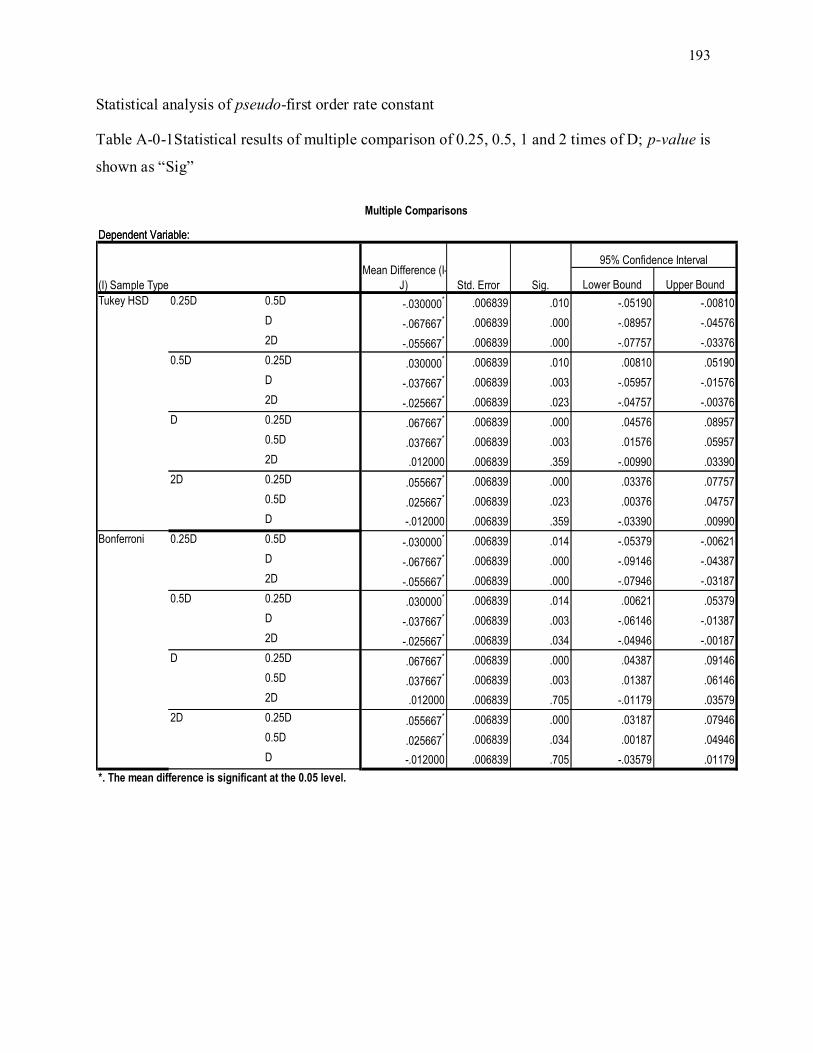
193
Statistical analysis of pseudo-first order rate constant
Table A-0-1Statistical results of multiple comparison of 0.25, 0.5, 1 and 2 times of D; p-value is
shown as “Sig”
Lower Bound Upper Bound
0.5D -.030000* .006839 .010 -.05190 -.00810
D -.067667* .006839 .000 -.08957 -.04576
2D -.055667* .006839 .000 -.07757 -.03376
0.25D .030000* .006839 .010 .00810 .05190
D -.037667* .006839 .003 -.05957 -.01576
2D -.025667* .006839 .023 -.04757 -.00376
0.25D .067667* .006839 .000 .04576 .08957
0.5D .037667* .006839 .003 .01576 .05957
2D .012000 .006839 .359 -.00990 .03390
0.25D .055667* .006839 .000 .03376 .07757
0.5D .025667* .006839 .023 .00376 .04757
D -.012000 .006839 .359 -.03390 .00990
0.5D -.030000* .006839 .014 -.05379 -.00621
D -.067667* .006839 .000 -.09146 -.04387
2D -.055667* .006839 .000 -.07946 -.03187
0.25D .030000* .006839 .014 .00621 .05379
D -.037667* .006839 .003 -.06146 -.01387
2D -.025667* .006839 .034 -.04946 -.00187
0.25D .067667* .006839 .000 .04387 .09146
0.5D .037667* .006839 .003 .01387 .06146
2D .012000 .006839 .705 -.01179 .03579
0.25D .055667* .006839 .000 .03187 .07946
0.5D .025667* .006839 .034 .00187 .04946
D -.012000 .006839 .705 -.03579 .01179
2D
Multiple Comparisons
Dependent Variable: Dependent Variable:
(I) Sample Type
Mean Difference (I-
J) Std. Error Sig.
95% Confidence Interval
*. The mean difference is significant at the 0.05 level.
Tukey HSD 0.25D
0.5D
D
2D
Bonferroni 0.25D
0.5D
D
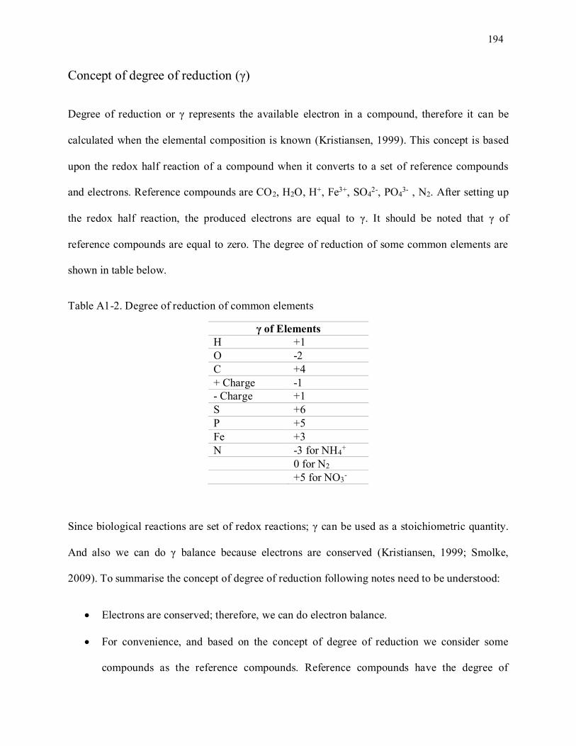
194
Concept of degree of reduction (γ)
Degree of reduction or γ represents the available electron in a compound, therefore it can be
calculated when the elemental composition is known (Kristiansen, 1999). This concept is based
upon the redox half reaction of a compound when it converts to a set of reference compounds
and electrons. Reference compounds are CO2, H2O, H+, Fe3+, SO42-, PO4
3- , N2. After setting up
the redox half reaction, the produced electrons are equal to γ. It should be noted that γ of
reference compounds are equal to zero. The degree of reduction of some common elements are
shown in table below.
Table A1-2. Degree of reduction of common elements
γ of Elements
H +1
O -2
C +4
+ Charge -1
- Charge +1
S +6
P +5
Fe +3
N -3 for NH4+
0 for N2
+5 for NO3-
Since biological reactions are set of redox reactions; γ can be used as a stoichiometric quantity.
And also we can do γ balance because electrons are conserved (Kristiansen, 1999; Smolke,
2009). To summarise the concept of degree of reduction following notes need to be understood:
Electrons are conserved; therefore, we can do electron balance.
For convenience, and based on the concept of degree of reduction we consider some
compounds as the reference compounds. Reference compounds have the degree of
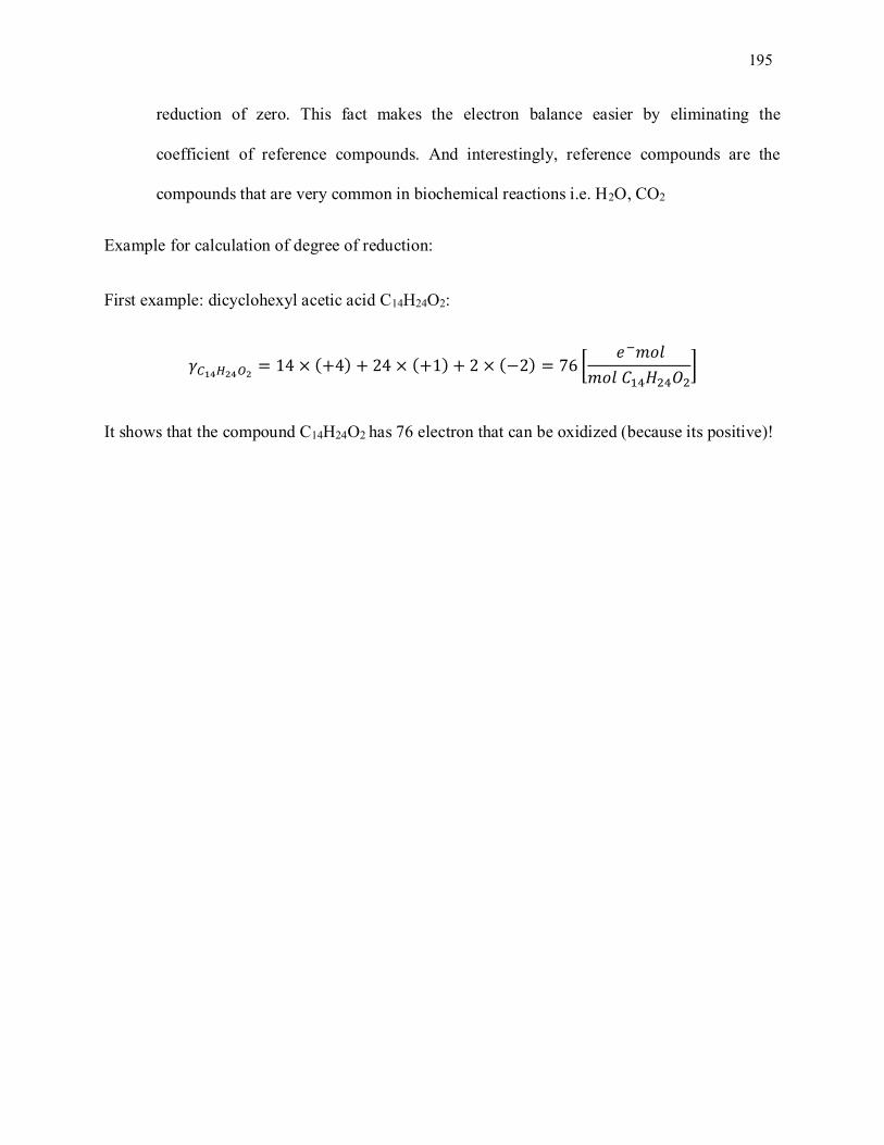
195
reduction of zero. This fact makes the electron balance easier by eliminating the
coefficient of reference compounds. And interestingly, reference compounds are the
compounds that are very common in biochemical reactions i.e. H2O, CO2
Example for calculation of degree of reduction:
First example: dicyclohexyl acetic acid C14H24O2:
𝛾𝐶14𝐻24𝑂2= 14 × (+4) + 24 × (+1) + 2 × (−2) = 76 [
𝑒−𝑚𝑜𝑙
𝑚𝑜𝑙 𝐶14𝐻24𝑂2]
It shows that the compound C14H24O2 has 76 electron that can be oxidized (because its positive)!

196
APPENDIX 2: SUPPLEMENTARY DATA FOR CHAPTER 4
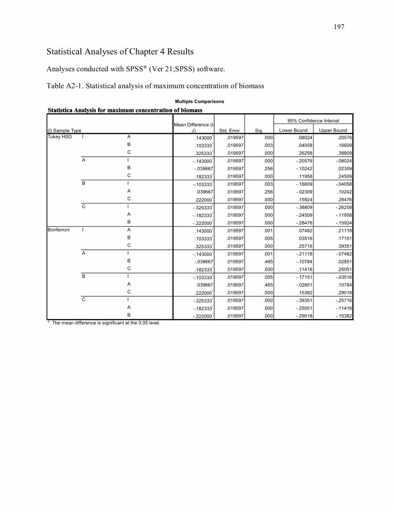
197
Statistical Analyses of Chapter 4 Results
Analyses conducted with SPSS® (Ver 21;SPSS) software.
Table A2-1. Statistical analysis of maximum concentration of biomass
Lower Bound Upper Bound
A .143000* .019597 .000 .08024 .20576
B .103333* .019597 .003 .04058 .16609
C .325333* .019597 .000 .26258 .38809
I -.143000* .019597 .000 -.20576 -.08024
B -.039667 .019597 .256 -.10242 .02309
C .182333* .019597 .000 .11958 .24509
I -.103333* .019597 .003 -.16609 -.04058
A .039667 .019597 .256 -.02309 .10242
C .222000* .019597 .000 .15924 .28476
I -.325333* .019597 .000 -.38809 -.26258
A -.182333* .019597 .000 -.24509 -.11958
B -.222000* .019597 .000 -.28476 -.15924
A .143000* .019597 .001 .07482 .21118
B .103333* .019597 .005 .03516 .17151
C .325333* .019597 .000 .25716 .39351
I -.143000* .019597 .001 -.21118 -.07482
B -.039667 .019597 .465 -.10784 .02851
C .182333* .019597 .000 .11416 .25051
I -.103333* .019597 .005 -.17151 -.03516
A .039667 .019597 .465 -.02851 .10784
C .222000* .019597 .000 .15382 .29018
I -.325333* .019597 .000 -.39351 -.25716
A -.182333* .019597 .000 -.25051 -.11416
B -.222000* .019597 .000 -.29018 -.15382
*. The mean difference is significant at the 0.05 level.
Tukey HSD I
A
B
C
Bonferroni I
A
B
C
Multiple Comparisons
Statistica Analysis for maximum concentration of biomassStatistica Analysis for maximum concentration of biomass
(I) Sample Type
Mean Difference (I-
J) Std. Error Sig.
95% Confidence Interval
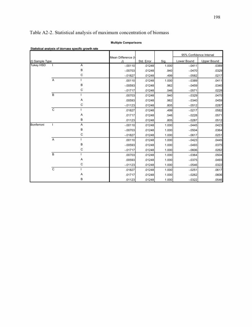
198
Table A2-2. Statistical analysis of maximum concentration of biomass
Lower Bound Upper Bound
A -.00110 .01248 1.000 -.0411 .0389
B -.00703 .01248 .940 -.0470 .0329
C -.01827 .01248 .499 -.0582 .0217
I .00110 .01248 1.000 -.0389 .0411
B -.00593 .01248 .962 -.0459 .0340
C -.01717 .01248 .546 -.0571 .0228
I .00703 .01248 .940 -.0329 .0470
A .00593 .01248 .962 -.0340 .0459
C -.01123 .01248 .805 -.0512 .0287
I .01827 .01248 .499 -.0217 .0582
A .01717 .01248 .546 -.0228 .0571
B .01123 .01248 .805 -.0287 .0512
A -.00110 .01248 1.000 -.0445 .0423
B -.00703 .01248 1.000 -.0504 .0364
C -.01827 .01248 1.000 -.0617 .0251
I .00110 .01248 1.000 -.0423 .0445
B -.00593 .01248 1.000 -.0493 .0375
C -.01717 .01248 1.000 -.0606 .0262
I .00703 .01248 1.000 -.0364 .0504
A .00593 .01248 1.000 -.0375 .0493
C -.01123 .01248 1.000 -.0546 .0322
I .01827 .01248 1.000 -.0251 .0617
A .01717 .01248 1.000 -.0262 .0606
B .01123 .01248 1.000 -.0322 .0546
Tukey HSD I
A
B
C
Bonferroni I
A
B
C
Multiple Comparisons
Statistical analysis of biomass specific growth rate Statistical analysis of biomass specific growth rate
(I) Sample Type
Mean Difference (I-
J) Std. Error Sig.
95% Confidence Interval
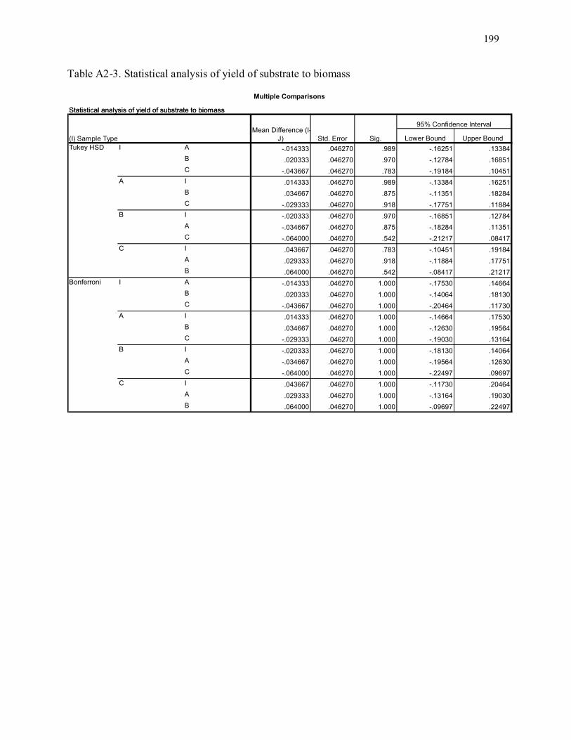
199
Table A2-3. Statistical analysis of yield of substrate to biomass
Lower Bound Upper Bound
A -.014333 .046270 .989 -.16251 .13384
B .020333 .046270 .970 -.12784 .16851
C -.043667 .046270 .783 -.19184 .10451
I .014333 .046270 .989 -.13384 .16251
B .034667 .046270 .875 -.11351 .18284
C -.029333 .046270 .918 -.17751 .11884
I -.020333 .046270 .970 -.16851 .12784
A -.034667 .046270 .875 -.18284 .11351
C -.064000 .046270 .542 -.21217 .08417
I .043667 .046270 .783 -.10451 .19184
A .029333 .046270 .918 -.11884 .17751
B .064000 .046270 .542 -.08417 .21217
A -.014333 .046270 1.000 -.17530 .14664
B .020333 .046270 1.000 -.14064 .18130
C -.043667 .046270 1.000 -.20464 .11730
I .014333 .046270 1.000 -.14664 .17530
B .034667 .046270 1.000 -.12630 .19564
C -.029333 .046270 1.000 -.19030 .13164
I -.020333 .046270 1.000 -.18130 .14064
A -.034667 .046270 1.000 -.19564 .12630
C -.064000 .046270 1.000 -.22497 .09697
I .043667 .046270 1.000 -.11730 .20464
A .029333 .046270 1.000 -.13164 .19030
B .064000 .046270 1.000 -.09697 .22497
Tukey HSD I
A
B
C
Bonferroni I
A
B
C
Multiple Comparisons
Statistical analysis of yield of substrate to biomassStatistical analysis of yield of substrate to biomass
(I) Sample Type
Mean Difference (I-
J) Std. Error Sig.
95% Confidence Interval
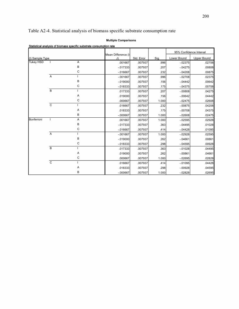
200
Table A2-4. Statistical analysis of biomass specific substrate consumption rate
Lower Bound Upper Bound
A .001667 .007937 .996 -.02375 .02708
B -.017333 .007937 .207 -.04275 .00808
C -.016667 .007937 .232 -.04208 .00875
I -.001667 .007937 .996 -.02708 .02375
B -.019000 .007937 .156 -.04442 .00642
C -.018333 .007937 .175 -.04375 .00708
I .017333 .007937 .207 -.00808 .04275
A .019000 .007937 .156 -.00642 .04442
C .000667 .007937 1.000 -.02475 .02608
I .016667 .007937 .232 -.00875 .04208
A .018333 .007937 .175 -.00708 .04375
B -.000667 .007937 1.000 -.02608 .02475
A .001667 .007937 1.000 -.02595 .02928
B -.017333 .007937 .363 -.04495 .01028
C -.016667 .007937 .414 -.04428 .01095
I -.001667 .007937 1.000 -.02928 .02595
B -.019000 .007937 .262 -.04661 .00861
C -.018333 .007937 .298 -.04595 .00928
I .017333 .007937 .363 -.01028 .04495
A .019000 .007937 .262 -.00861 .04661
C .000667 .007937 1.000 -.02695 .02828
I .016667 .007937 .414 -.01095 .04428
A .018333 .007937 .298 -.00928 .04595
B -.000667 .007937 1.000 -.02828 .02695
Tukey HSD I
A
B
C
Bonferroni I
A
B
C
Multiple Comparisons
Statistical analysis of biomass specific substrate consumption rate Statistical analysis of biomass specific substrate consumption rate
(I) Sample Type
Mean Difference (I-
J) Std. Error Sig.
95% Confidence Interval
201
THEORETICAL APPROACH TO CALCULATE OXYGEN CONSUMPTION RATE
Following approach can be used to approximate the rate of oxygen consumption in the system.
First of all we need to know the degree of reduction of substrate per C-atom. Since here
determination of exact amount of degree of reduction was not possible because of lack of
accurate formula for the substrate. To debottleneck this issue, an experimental approach based on
concept of COD and TOC has been used to calculate the degree of reduction of substrate.
After determination of degree of reduction of substrate, yield of electron acceptor can be
obtained through setting up a redox balance. It should be noted that for convenience in writing
the redox balance, degree of reduction of reaction constituents is considered as zero except
electron donor, electron acceptor and biomass. Further explanation can be found in chapter 5 of
this thesis.
Order of materials is as follows:
1. Determination of degree of reduction of substrate per C-atom
a. Calculation of COD based on degree of reduction
b. Calculation of TOC
c. Correlation for degree of reduction and TOC and COD
2. Setting up redox balance among electron donor, electron acceptor and biomass
a. Redox balance
b. Yield of electron acceptor to biomass (𝑌𝐴𝑋)
c. Conversion of yield to biomass specific oxygen consumption rate
Calculation of degree of reduction of substrate
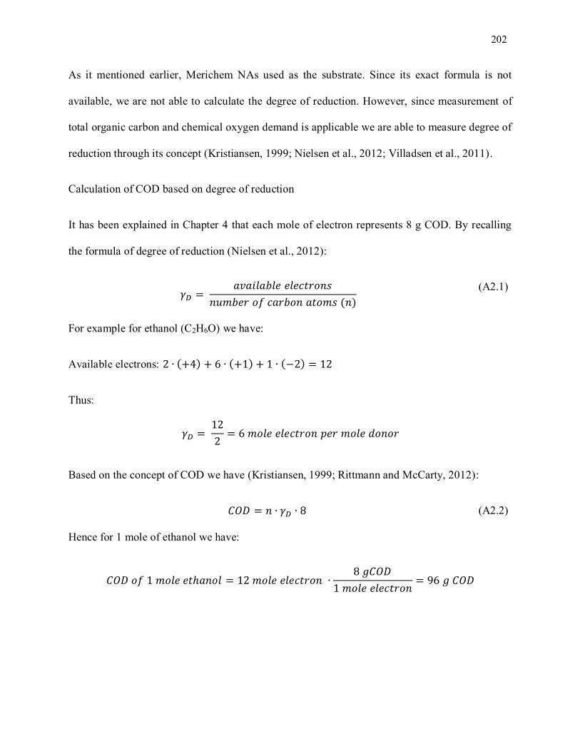
202
As it mentioned earlier, Merichem NAs used as the substrate. Since its exact formula is not
available, we are not able to calculate the degree of reduction. However, since measurement of
total organic carbon and chemical oxygen demand is applicable we are able to measure degree of
reduction through its concept (Kristiansen, 1999; Nielsen et al., 2012; Villadsen et al., 2011).
Calculation of COD based on degree of reduction
It has been explained in Chapter 4 that each mole of electron represents 8 g COD. By recalling
the formula of degree of reduction (Nielsen et al., 2012):
𝛾𝐷 = 𝑎𝑣𝑎𝑖𝑙𝑎𝑏𝑙𝑒 𝑒𝑙𝑒𝑐𝑡𝑟𝑜𝑛𝑠
𝑛𝑢𝑚𝑏𝑒𝑟 𝑜𝑓 𝑐𝑎𝑟𝑏𝑜𝑛 𝑎𝑡𝑜𝑚𝑠 (𝑛)
(A2.1)
For example for ethanol (C2H6O) we have:
Available electrons: 2 ∙ (+4) + 6 ∙ (+1) + 1 ∙ (−2) = 12
Thus:
𝛾𝐷 = 12
2= 6 𝑚𝑜𝑙𝑒 𝑒𝑙𝑒𝑐𝑡𝑟𝑜𝑛 𝑝𝑒𝑟 𝑚𝑜𝑙𝑒 𝑑𝑜𝑛𝑜𝑟
Based on the concept of COD we have (Kristiansen, 1999; Rittmann and McCarty, 2012):
𝐶𝑂𝐷 = 𝑛 ∙ 𝛾𝐷 ∙ 8 (A2.2)
Hence for 1 mole of ethanol we have:
𝐶𝑂𝐷 𝑜𝑓 1 𝑚𝑜𝑙𝑒 𝑒𝑡ℎ𝑎𝑛𝑜𝑙 = 12 𝑚𝑜𝑙𝑒 𝑒𝑙𝑒𝑐𝑡𝑟𝑜𝑛 ∙8 𝑔𝐶𝑂𝐷
1 𝑚𝑜𝑙𝑒 𝑒𝑙𝑒𝑐𝑡𝑟𝑜𝑛= 96 𝑔 𝐶𝑂𝐷
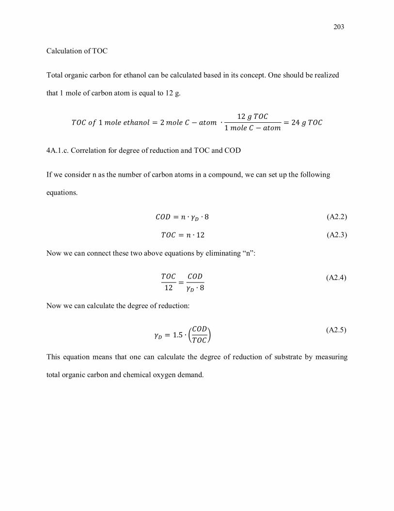
203
Calculation of TOC
Total organic carbon for ethanol can be calculated based in its concept. One should be realized
that 1 mole of carbon atom is equal to 12 g.
𝑇𝑂𝐶 𝑜𝑓 1 𝑚𝑜𝑙𝑒 𝑒𝑡ℎ𝑎𝑛𝑜𝑙 = 2 𝑚𝑜𝑙𝑒 𝐶 − 𝑎𝑡𝑜𝑚 ∙12 𝑔 𝑇𝑂𝐶
1 𝑚𝑜𝑙𝑒 𝐶 − 𝑎𝑡𝑜𝑚= 24 𝑔 𝑇𝑂𝐶
4A.1.c. Correlation for degree of reduction and TOC and COD
If we consider n as the number of carbon atoms in a compound, we can set up the following
equations.
𝐶𝑂𝐷 = 𝑛 ∙ 𝛾𝐷 ∙ 8 (A2.2)
𝑇𝑂𝐶 = 𝑛 ∙ 12 (A2.3)
Now we can connect these two above equations by eliminating “n”:
𝑇𝑂𝐶
12=
𝐶𝑂𝐷
𝛾𝐷 ∙ 8
(A2.4)
Now we can calculate the degree of reduction:
𝛾𝐷 = 1.5 ∙ (𝐶𝑂𝐷
𝑇𝑂𝐶)
(A2.5)
This equation means that one can calculate the degree of reduction of substrate by measuring
total organic carbon and chemical oxygen demand.
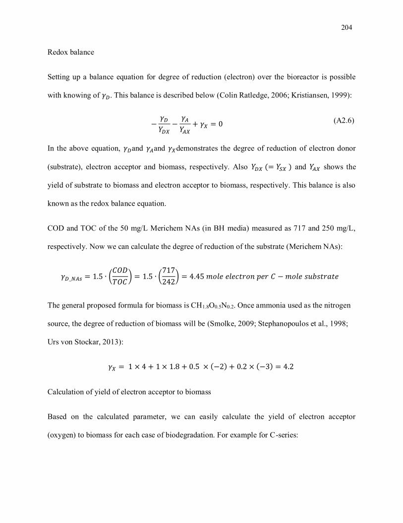
204
Redox balance
Setting up a balance equation for degree of reduction (electron) over the bioreactor is possible
with knowing of 𝛾𝐷. This balance is described below (Colin Ratledge, 2006; Kristiansen, 1999):
−𝛾𝐷
𝑌𝐷𝑋−
𝛾𝐴
𝑌𝐴𝑋+ 𝛾𝑋 = 0
(A2.6)
In the above equation, 𝛾𝐷and 𝛾𝐴and 𝛾𝑋demonstrates the degree of reduction of electron donor
(substrate), electron acceptor and biomass, respectively. Also 𝑌𝐷𝑋 (= 𝑌𝑆𝑋 ) and 𝑌𝐴𝑋 shows the
yield of substrate to biomass and electron acceptor to biomass, respectively. This balance is also
known as the redox balance equation.
COD and TOC of the 50 mg/L Merichem NAs (in BH media) measured as 717 and 250 mg/L,
respectively. Now we can calculate the degree of reduction of the substrate (Merichem NAs):
𝛾𝐷_𝑁𝐴𝑠 = 1.5 ∙ (𝐶𝑂𝐷
𝑇𝑂𝐶) = 1.5 ∙ (
717
242) = 4.45 𝑚𝑜𝑙𝑒 𝑒𝑙𝑒𝑐𝑡𝑟𝑜𝑛 𝑝𝑒𝑟 𝐶 − 𝑚𝑜𝑙𝑒 𝑠𝑢𝑏𝑠𝑡𝑟𝑎𝑡𝑒
The general proposed formula for biomass is CH1.8O0.5N0.2. Once ammonia used as the nitrogen
source, the degree of reduction of biomass will be (Smolke, 2009; Stephanopoulos et al., 1998;
Urs von Stockar, 2013):
𝛾𝑋 = 1 × 4 + 1 × 1.8 + 0.5 × (−2) + 0.2 × (−3) = 4.2
Calculation of yield of electron acceptor to biomass
Based on the calculated parameter, we can easily calculate the yield of electron acceptor
(oxygen) to biomass for each case of biodegradation. For example for C-series:
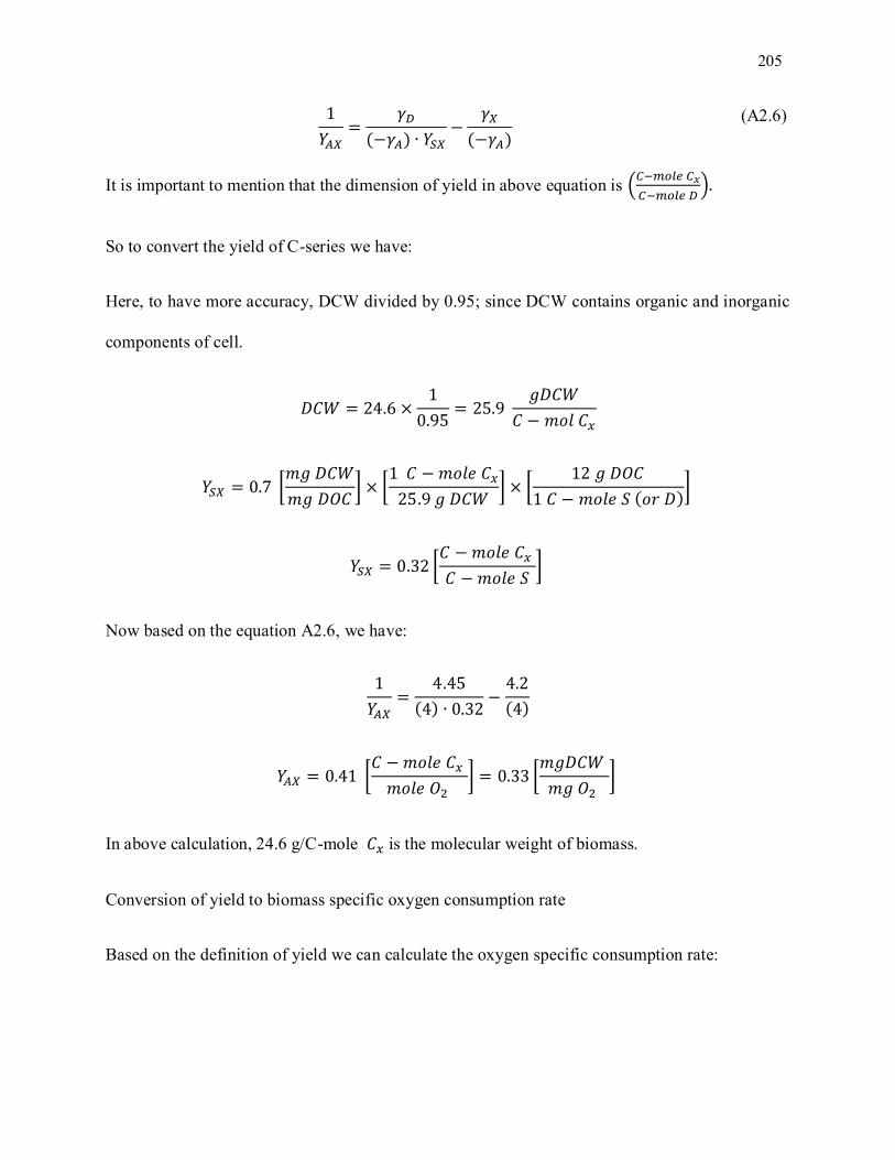
205
1
𝑌𝐴𝑋=
𝛾𝐷
(−𝛾𝐴) ∙ 𝑌𝑆𝑋−
𝛾𝑋
(−𝛾𝐴)
(A2.6)
It is important to mention that the dimension of yield in above equation is (𝐶−𝑚𝑜𝑙𝑒 𝐶𝑥
𝐶−𝑚𝑜𝑙𝑒 𝐷).
So to convert the yield of C-series we have:
Here, to have more accuracy, DCW divided by 0.95; since DCW contains organic and inorganic
components of cell.
𝐷𝐶𝑊 = 24.6 ×1
0.95= 25.9
𝑔𝐷𝐶𝑊
𝐶 − 𝑚𝑜𝑙 𝐶𝑥
𝑌𝑆𝑋 = 0.7 [𝑚𝑔 𝐷𝐶𝑊
𝑚𝑔 𝐷𝑂𝐶] × [
1 𝐶 − 𝑚𝑜𝑙𝑒 𝐶𝑥
25.9 𝑔 𝐷𝐶𝑊] × [
12 𝑔 𝐷𝑂𝐶
1 𝐶 − 𝑚𝑜𝑙𝑒 𝑆 (𝑜𝑟 𝐷)]
𝑌𝑆𝑋 = 0.32 [𝐶 − 𝑚𝑜𝑙𝑒 𝐶𝑥
𝐶 − 𝑚𝑜𝑙𝑒 𝑆]
Now based on the equation A2.6, we have:
1
𝑌𝐴𝑋
=4.45
(4) ∙ 0.32−
4.2
(4)
𝑌𝐴𝑋 = 0.41 [𝐶 − 𝑚𝑜𝑙𝑒 𝐶𝑥
𝑚𝑜𝑙𝑒 𝑂2 ] = 0.33 [
𝑚𝑔𝐷𝐶𝑊
𝑚𝑔 𝑂2 ]
In above calculation, 24.6 g/C-mole 𝐶𝑥 is the molecular weight of biomass.
Conversion of yield to biomass specific oxygen consumption rate
Based on the definition of yield we can calculate the oxygen specific consumption rate:
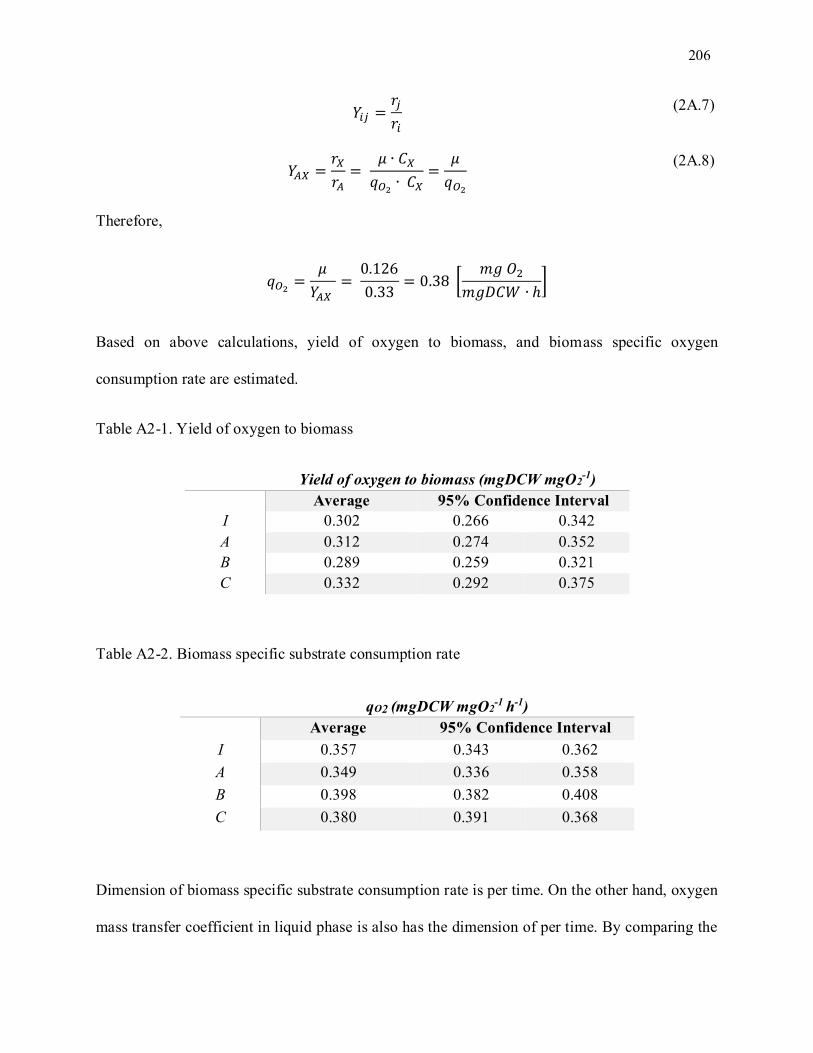
206
𝑌𝑖𝑗 =𝑟𝑗
𝑟𝑖
(2A.7)
𝑌𝐴𝑋 =𝑟𝑋
𝑟𝐴=
𝜇 ∙ 𝐶𝑋
𝑞𝑂2∙ 𝐶𝑋
=𝜇
𝑞𝑂2
(2A.8)
Therefore,
𝑞𝑂2=
𝜇
𝑌𝐴𝑋 =
0.126
0.33= 0.38 [
𝑚𝑔 𝑂2
𝑚𝑔𝐷𝐶𝑊 ∙ ℎ]
Based on above calculations, yield of oxygen to biomass, and biomass specific oxygen
consumption rate are estimated.
Table A2-1. Yield of oxygen to biomass
Yield of oxygen to biomass (mgDCW mgO2-1)
Average 95% Confidence Interval
I 0.302 0.266 0.342
A 0.312 0.274 0.352
B 0.289 0.259 0.321
C 0.332 0.292 0.375
Table A2-2. Biomass specific substrate consumption rate
qO2 (mgDCW mgO2-1 h-1)
Average 95% Confidence Interval
I 0.357 0.343 0.362
A 0.349 0.336 0.358
B 0.398 0.382 0.408
C 0.380 0.391 0.368
Dimension of biomass specific substrate consumption rate is per time. On the other hand, oxygen
mass transfer coefficient in liquid phase is also has the dimension of per time. By comparing the

207
oxygen mass transfer coefficient in liquid phase which changes from 11 to 28.5 h -1 to biomass
specific oxygen consumption rate; it can be seen that oxygen was not a limiting factor through
the experiment.

208
APPENDIX 3: SUPPLEMENTARY DATA FOR CHAPTER 5
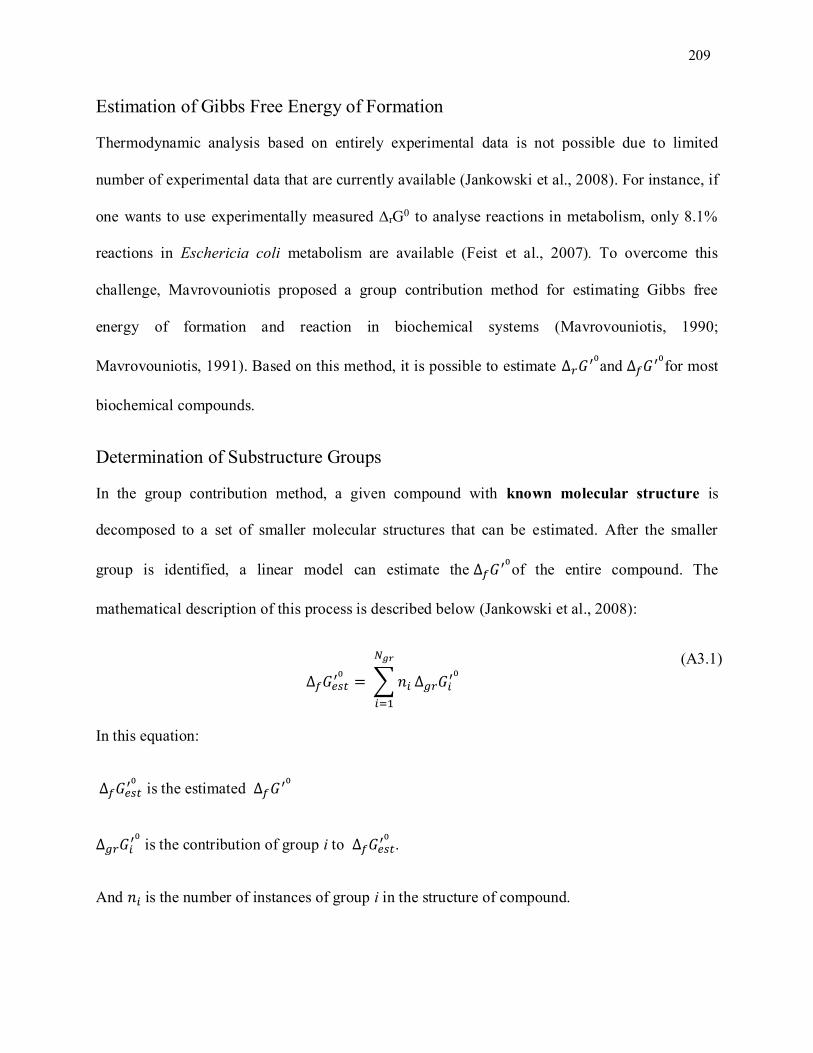
209
Estimation of Gibbs Free Energy of Formation
Thermodynamic analysis based on entirely experimental data is not possible due to limited
number of experimental data that are currently available (Jankowski et al., 2008). For instance, if
one wants to use experimentally measured ∆rG0 to analyse reactions in metabolism, only 8.1%
reactions in Eschericia coli metabolism are available (Feist et al., 2007). To overcome this
challenge, Mavrovouniotis proposed a group contribution method for estimating Gibbs free
energy of formation and reaction in biochemical systems (Mavrovouniotis, 1990;
Mavrovouniotis, 1991). Based on this method, it is possible to estimate ∆𝑟𝐺′0and ∆𝑓𝐺
′0for most
biochemical compounds.
Determination of Substructure Groups
In the group contribution method, a given compound with known molecular structure is
decomposed to a set of smaller molecular structures that can be estimated. After the smaller
group is identified, a linear model can estimate the ∆𝑓𝐺′0of the entire compound. The
mathematical description of this process is described below (Jankowski et al., 2008):
∆𝑓𝐺𝑒𝑠𝑡′0 = ∑ 𝑛𝑖
𝑁𝑔𝑟
𝑖=1
∆𝑔𝑟𝐺𝑖′0
(A3.1)
In this equation:
∆𝑓𝐺𝑒𝑠𝑡′0 is the estimated ∆𝑓𝐺
′0
∆𝑔𝑟𝐺𝑖′0 is the contribution of group i to ∆𝑓𝐺𝑒𝑠𝑡
′0 .
And 𝑛𝑖 is the number of instances of group i in the structure of compound.
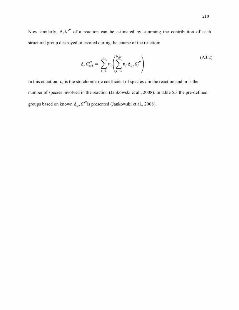
210
Now similarly, ∆𝑟𝐺′0 of a reaction can be estimated by summing the contribution of each
structural group destroyed or created during the course of the reaction:
∆𝑟𝐺𝑒𝑠𝑡′0 = ∑ 𝑣𝑖
𝑚
𝑖=1
(∑ 𝑛𝑗
𝑁𝑔𝑟
𝑗=1
∆𝑔𝑟𝐺𝑗′0)
(A3.2)
In this equation, 𝑣𝑖 is the stoichiometric coefficient of species i in the reaction and m is the
number of species involved in the reaction (Jankowski et al., 2008). In table 5.3 the pre-defined
groups based on known ∆𝑔𝑟𝐺′0is presented (Jankowski et al., 2008).
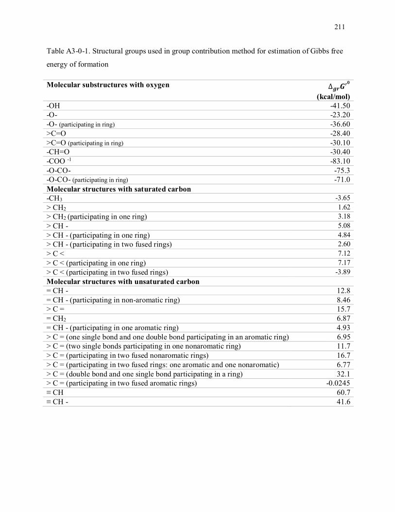
211
Table A3-0-1. Structural groups used in group contribution method for estimation of Gibbs free
energy of formation
Molecular substructures with oxygen ∆𝒈𝒓𝑮′𝟎
(kcal/mol)
-OH -41.50
-O- -23.20
-O- (participating in ring) -36.60
>C=O -28.40
>C=O (participating in ring) -30.10
-CH=O -30.40
-COO -1 -83.10
-O-CO- -75.3
-O-CO- (participating in ring) -71.0
Molecular structures with saturated carbon
-CH3 -3.65
> CH2 1.62
> CH2 (participating in one ring) 3.18
> CH - 5.08
> CH - (participating in one ring) 4.84
> CH - (participating in two fused rings) 2.60
> C < 7.12
> C < (participating in one ring) 7.17
> C < (participating in two fused rings) -3.89
Molecular structures with unsaturated carbon
= CH - 12.8
= CH - (participating in non-aromatic ring) 8.46
> C = 15.7
= CH2 6.87
= CH - (participating in one aromatic ring) 4.93
> C = (one single bond and one double bond participating in an aromatic ring) 6.95
> C = (two single bonds participating in one nonaromatic ring) 11.7
> C = (participating in two fused nonaromatic rings) 16.7
> C = (participating in two fused rings: one aromatic and one nonaromatic) 6.77
> C = (double bond and one single bond participating in a ring) 32.1
> C = (participating in two fused aromatic rings) -0.0245
≡ CH 60.7
≡ CH - 41.6
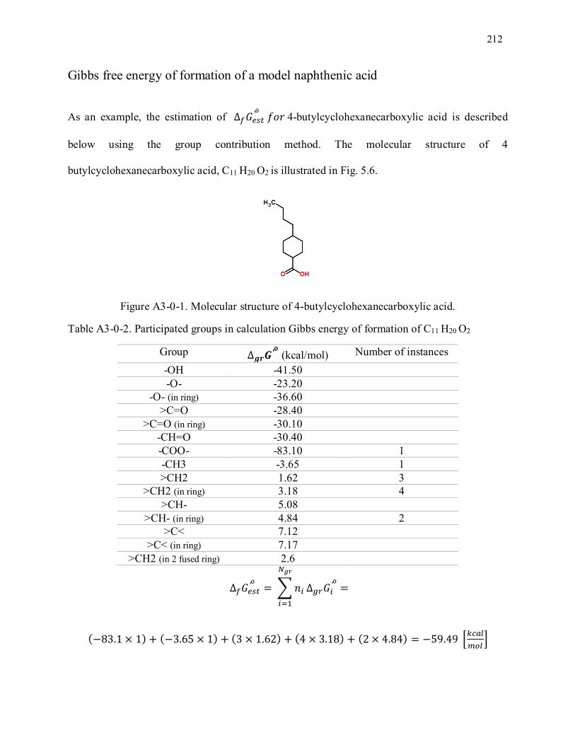
212
Gibbs free energy of formation of a model naphthenic acid
As an example, the estimation of ∆𝑓𝐺𝑒𝑠𝑡′0
𝑓𝑜𝑟 4-butylcyclohexanecarboxylic acid is described
below using the group contribution method. The molecular structure of 4
butylcyclohexanecarboxylic acid, C11 H20 O2 is illustrated in Fig. 5.6.
Figure A3-0-1. Molecular structure of 4-butylcyclohexanecarboxylic acid.
Table A3-0-2. Participated groups in calculation Gibbs energy of formation of C11 H20 O2
Group ∆𝒈𝒓𝑮′𝟎 (kcal/mol) Number of instances
-OH -41.50
-O- -23.20
-O- (in ring) -36.60
>C=O -28.40
>C=O (in ring) -30.10
-CH=O -30.40
-COO- -83.10 1
-CH3 -3.65 1
>CH2 1.62 3
>CH2 (in ring) 3.18 4
>CH- 5.08
>CH- (in ring) 4.84 2
>C< 7.12
>C< (in ring) 7.17
>CH2 (in 2 fused ring) 2.6
∆𝑓𝐺𝑒𝑠𝑡′0
= ∑ 𝑛𝑖
𝑁𝑔𝑟
𝑖=1
∆𝑔𝑟𝐺𝑖′0
=
(−83.1 × 1) + (−3.65 × 1) + (3 × 1.62) + (4 × 3.18) + (2 × 4.84) = −59.49 [𝑘𝑐𝑎𝑙
𝑚𝑜𝑙]
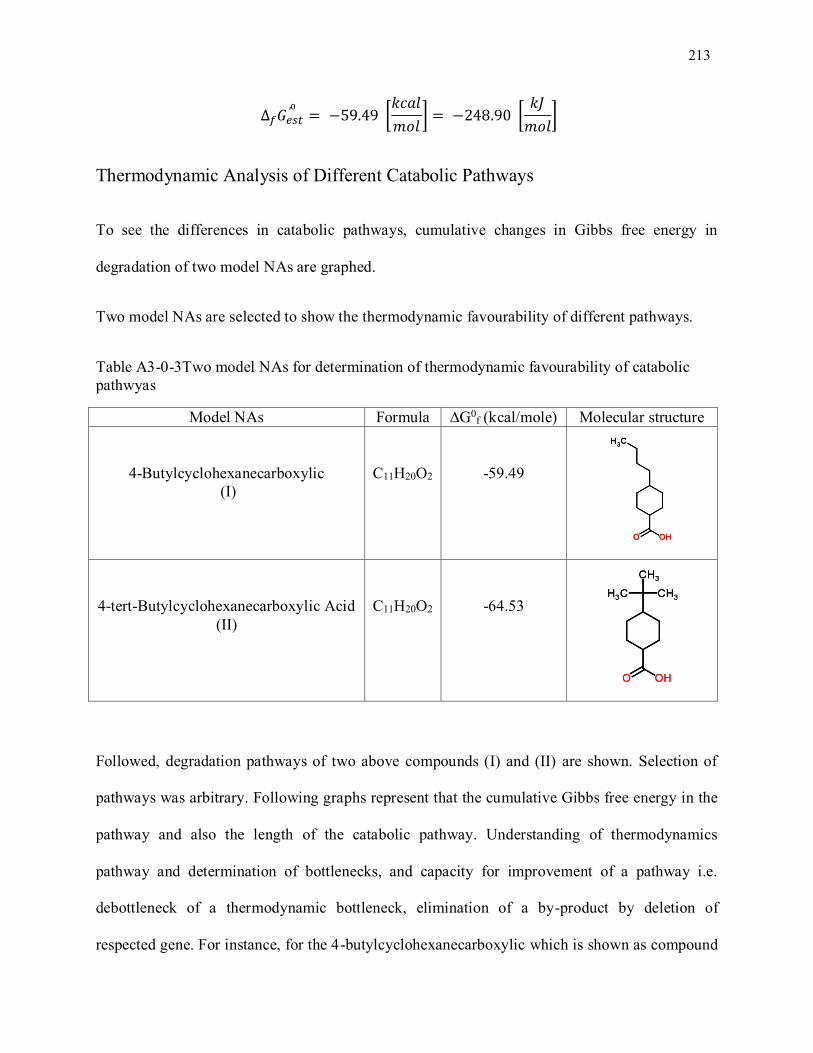
213
∆𝑓𝐺𝑒𝑠𝑡′0
= −59.49 [𝑘𝑐𝑎𝑙
𝑚𝑜𝑙] = −248.90 [
𝑘𝐽
𝑚𝑜𝑙]
Thermodynamic Analysis of Different Catabolic Pathways
To see the differences in catabolic pathways, cumulative changes in Gibbs free energy in
degradation of two model NAs are graphed.
Two model NAs are selected to show the thermodynamic favourability of different pathways.
Table A3-0-3Two model NAs for determination of thermodynamic favourability of catabolic
pathwyas
Model NAs Formula ∆G0f (kcal/mole) Molecular structure
4-Butylcyclohexanecarboxylic
(I)
C11H20O2
-59.49
4-tert-Butylcyclohexanecarboxylic Acid
(II)
C11H20O2
-64.53
Followed, degradation pathways of two above compounds (I) and (II) are shown. Selection of
pathways was arbitrary. Following graphs represent that the cumulative Gibbs free energy in the
pathway and also the length of the catabolic pathway. Understanding of thermodynamics
pathway and determination of bottlenecks, and capacity for improvement of a pathway i.e.
debottleneck of a thermodynamic bottleneck, elimination of a by-product by deletion of
respected gene. For instance, for the 4-butylcyclohexanecarboxylic which is shown as compound

214
(I): the pathway 1 is shorter than pathway 2, in spite of the fact that they can have same end
product (which result in the same Gibb free energy changes), pathway 2 is more
thermodynamically favourable.
.
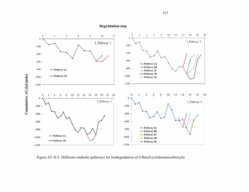
215
. Figure A3 -0-2. Different catabolic pathways for biodegradation of 4-Butylcyclohexanecarboxylic
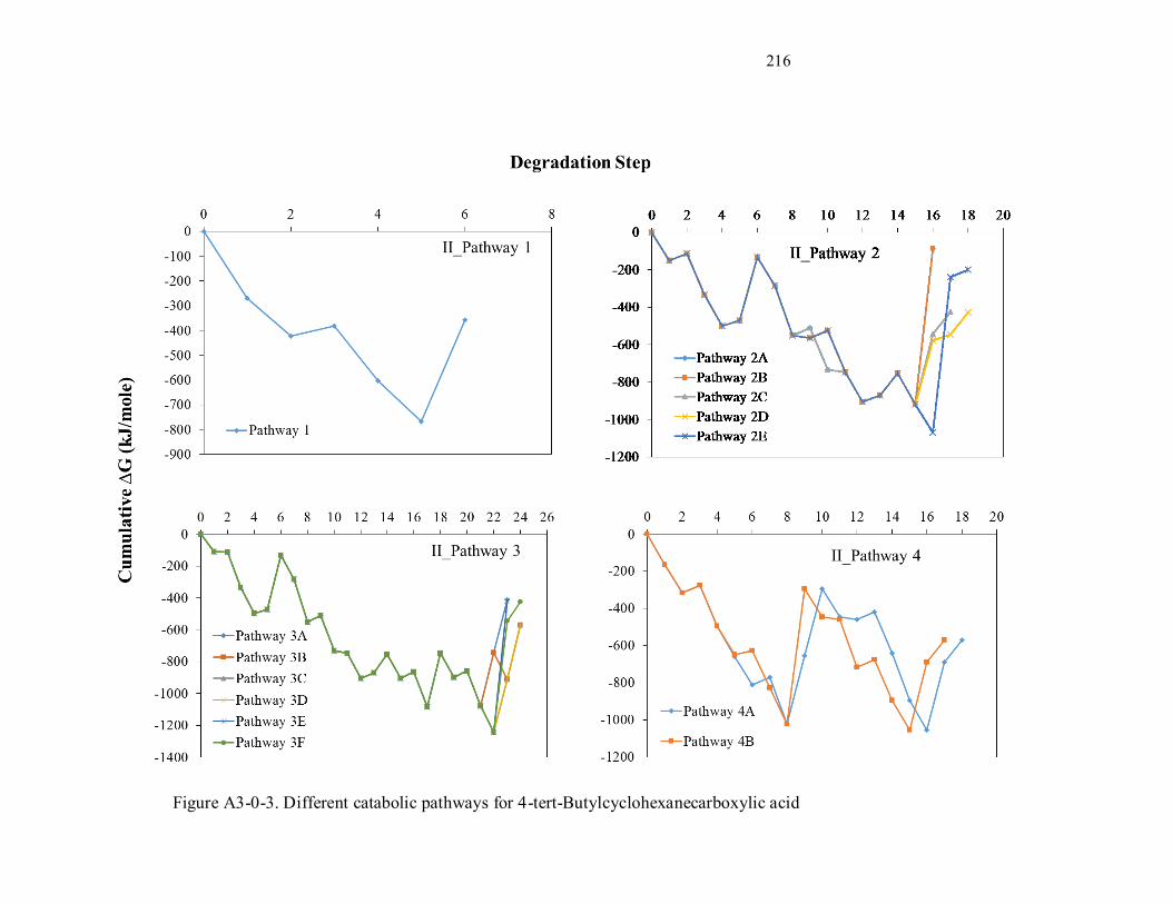
216
Figure A3-0-3. Different catabolic pathways for 4-tert-Butylcyclohexanecarboxylic acid
217
Another interesting result can be obtained by comparison of pathway 1 and 2 for compound II.
Due to cumulative Gibbs free energy, it can be seen that pathway 2 of compound II is more
favourable, however the last step is a huge thermodynamic bottleneck. It might be a possibility
that a wild type microorganism(s) cannot overcome this issue. Therefore, pathway analyses
create opportunities for improvement of biodegradation by engineered microorganisms.


![Green Demulsifier Development - Proserv...III Demulsifier Chemistry History Time period Dosage [ppm] Chemistry 1920 - 1935 500 - 1.000 Naphthenic acids, aromatic and aliphatic sulphonates](https://img.pdfslide.net/doc/110x75/5e98b35e13d8180128073d18/green-demulsifier-development-proserv-iii-demulsifier-chemistry-history-time.jpg)