Embed Size (px)
Citation preview
The Pennsylvania State University
The Graduate School
CHEMICAL COMBUSTION POWER SYSTEMS FOR EXTREME
ENVIRONMENT PLANETARY LANDERS
A Dissertation in
Mechanical Engineering
by
Christopher J. Greer
2021 Christopher J. Greer
Submitted in Partial Fulfillment
of the Requirements
for the Degree of
Doctor of Philosophy
May 2021
ii
The dissertation of Christopher J. Greer was reviewed and approved by the following:
Alexander S. Rattner
Dissertation Adviser, Chair of Committee
Dorothy Quiggle Career Development Professor Assistant Professor of Mechanical Engineering
Stephen P. Lynch
Committee Member
Associate Professor of Mechanical Engineering
Michael P. Manahan
Committee Member
Assistant Research Professor of Mechanical Engineering
James F. Kasting
External Committee Member
Distinguished Professor of Geosciences
Karen A. Thole
Head of the Department of Mechanical Engineering
Distinguished Professor of Mechanical Engineering
iii
Abstract
The extreme environments and low solar availability on the surfaces of Venus and Europa
translate to significant power and thermal management challenges for planetary lander missions.
The longest lasting mission to the surface of Venus was Venera 13 with a mission duration of 127
hours. To increase this mission duration, future missions will require power systems with greater
specific energy to enable active cooling. In-situ reactant-using metal combustion power systems
have been proposed as promising solutions but have not yet been analyzed in detail or
experimentally demonstrated and characterized.
In this dissertation, a detailed thermodynamic and heat transfer model of a conceptual lithium
combustion power system is first formulated. This analysis finds that a lithium combustion power
system using in-situ atmospheric carbon dioxide as an oxidizer could power a Venus lander with
14 kWth of thermal energy for five days with 185 kg of fuel. Even greater mission durations are
possible if lower power missions are considered. The potential performances of a lithium and
carbon-dioxide powered Stirling engine and sulfur-sodium batteries are compared. It is found that
sulfur-sodium batteries would require about 176% to 246% more mass to provide 1 kW of power
output for mission durations of five to ten days, respectively. A lithium combustion power system
with a sulfur-hexafluoride oxidizer is also analyzed for a Europa lander. This system could provide
94 W of power for up to twenty days with 43 kg of reactants mass.
Lithium and carbon-dioxide combustion tests are performed to characterize the practical yield
of lithium fuel and the heat of combustion from the reaction. Lithium yield estimates are found to
range over ~42 – 98%, depending on operating conditions. Based on these data, future in-situ
reactant using-lithium combustion powered missions to Venus and Mars could achieve a fuel
specific energy of ~25.6 MJ kg-1.
iv
To convert this thermal energy to cooling and electrical power, heat engines are compared for
conceptual Venus surface missions. A Rankine cycle with metal (mercury) working fluid is
proposed as a high-performance alternative to gas-cycle or solid-state heat engines. A
thermodynamic cycle model was developed and indicated that a mercury vapor Rankine cycle can
meet the power needs of future Venus landers with active refrigeration if supplied 12.3 kW of
thermal input. At feasible component performance levels, this system could provide 2.0 kW of
shaft work with an overall power efficiency of 16%. This shows the Rankine cycle meets the
performance requirements to supply enough power for a Venus lander when coupled with a
chemical combustion power system.
A mercury vapor Rankine cycle test stand has been built and testing is in process to validate
the system in a 300°C environment. The design for each component was presented and the
assembled test stand presented. Short duration steam operations have been performed, and
modifications are suggested before mercury operations are performed to address technical
challenges, primarily with the expander (turbine). Future work will compare performance with the
developed model and findings assessed to identify the most impactful improvements for future
system maturation efforts.
v
Table of Contents
LIST OF FIGURES ..................................................................................................................... viii
LIST OF TABLES ........................................................................................................................ xii
Acknowledgements ...................................................................................................................... xiii
Chapter 1 Introduction and Literature Review ......................................................................... 1
1.1. Extreme environment power and cooling challenges ......................................................... 2
1.2. Literature review ................................................................................................................. 6
1.2.1. Venus surface lander concept ................................................................................... 6
1.2.2. Europa lander concept .............................................................................................. 9
1.2.3. Potential in-situ lithium combustion with the Martian atmosphere ....................... 11
1.2.4. High temperature planetary lander heat engines .................................................... 12
1.3. Contributions and objectives of this Ph.D. dissertation research...................................... 13
Chapter 2 Analysis of Lithium Combustion Power Systems for Extreme Environment
Spacecraft .............................................................................................................. 15
2.1. Model formulation ............................................................................................................ 19
2.1.1. Control volume analysis ......................................................................................... 19
2.1.2. Baseline condition .................................................................................................. 22
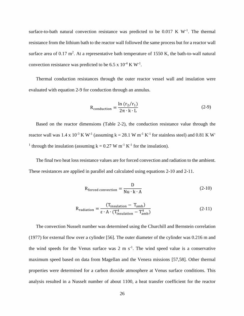
2.1.3. Thermal resistance network .................................................................................... 23
2.1.4. Natural convection in a lithium bath ...................................................................... 28
2.1.5. Sodium pool boiling in the thermosiphon .............................................................. 29
2.2. Data and results ................................................................................................................. 30
2.2.1. Venus mission with carbon dioxide oxidizer ......................................................... 30
2.2.2. Europa mission with sulfur-hexafluoride oxidizer ................................................. 33
2.2.3. Limitations of proposed model and future research needs ..................................... 36
2.3. Conclusion ........................................................................................................................ 37
2.3.1. Engineering Requirements ..................................................................................... 38
Chapter 3 Experimental Characterization of Lithium-Carbon Dioxide Combustion in
Batch Reactors for Powering Venus Landers .................................................... 40
3.1. Present investigation and objectives ................................................................................. 43
3.2. Lithium-carbon dioxide combustion experiments ............................................................ 44
3.2.1. Experimental facility and instrumentation ............................................................. 44
3.2.2. Experimental procedure ......................................................................................... 49
3.3. Results of lithium-carbon dioxide combustion experiments ............................................ 50
vi
3.3.1. Reactor 1.0: headspace reaction, internal air-cooling, 500°C Li bath .................... 51
3.3.2. Reactor 2.0: submerged injectors, external cooling ............................................... 55
3.3.3. Reactor 3.0: headspace reaction, external cooling, 700°C Li bath......................... 58
3.3.4. Reactor 3.1: headspace reaction, external cooling, 750°C Li bath, wick ............... 61
3.3.5. Reactor 3.2: Headspace reaction, external cooling, 900°C Li bath ........................ 63
3.4. Quantitative reaction analysis ........................................................................................... 65
3.4.1. CT scan processing ................................................................................................. 65
3.4.2. Quantifying reaction completion and effective fuel-specific energy ..................... 68
3.5. Conclusion ........................................................................................................................ 71
Chapter 4 Thermodynamic Analysis of a Mercury Vapor Rankine Cycle for a Venus
Lander ................................................................................................................... 73
4.1. Heat engine selection for Venus application .................................................................... 74
4.1.1. Metal vapor Rankine cycle ..................................................................................... 77
4.2. Mercury Vapor Rankine Cycle Thermodynamic Analysis ............................................... 77
4.2.1. Venus surface performance .................................................................................... 79
4.2.2. Lab scale model performance ................................................................................. 81
4.3. Conclusion….. .................................................................................................................. 82
4.3.1.Engineering Requirements ....................................................................................... 83
Chapter 5 Experimental Mercury Vapor Rankine Cycle Testing for a Venus Lander ....... 85
5.1. Experimental test stand ..................................................................................................... 86
5.2. Evaporator ......................................................................................................................... 91
5.3. Condenser ......................................................................................................................... 92
5.4. Reservoir and pump .......................................................................................................... 93
5.5. Turbine .............................................................................................................................. 95
5.6. Instrumentation ................................................................................................................. 96
5.7. Operation and Safety......................................................................................................... 96
5.8. Mercury vapor expander design selection ........................................................................ 97
5.8.1. Mercury RVE designs ............................................................................................ 99
5.8.2. Rankine cycle challenges ..................................................................................... 103
5.9. Future work ..................................................................................................................... 104
5.10.Conclusion ...................................................................................................................... 106
Chapter 6 Conclusions and Recommendations for Future Research .................................. 108
6.1. Lithium and carbon-dioxide, batch reactor modeling and experiments ......................... 109
vii
6.2. Mercury vapor Rankine cycle analysis and testing ......................................................... 110
6.3. Recommendations for future research ............................................................................ 110
Bibliography.. ............................................................................................................................. 112
Appendix: Uncertainty Analysis ................................................................................................. 128
viii
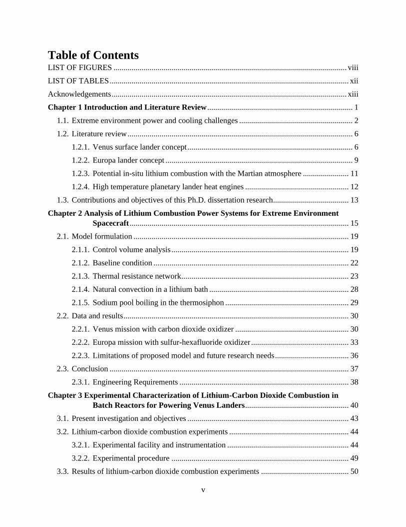
LIST OF FIGURES Figure 1-1: Thermal specific energy and power comparison for spacecraft power ....................... 4
Figure 1-2: Electrical specific energy and power comparison for spacecraft power ...................... 5
Figure 1-3: Lithium, carbon dioxide combustion power plant for a Venus lander ........................ 8
Figure 1-4: Lithium, sulfur hexafluoride combustion power plant for a Europa lander ............... 11
Figure 1-5: ALIVE concept Stirling duplex cycle ........................................................................ 13
Figure 2-1: Li/CO2 Power System Block Diagram for ALIVE Mission ...................................... 17
Figure 2-2: ALIVE Lander Concept with Highlighted Power System Components [15] ............ 17
Figure 2-3: Li/SF6 Power System Block Diagram for Europa Lander ......................................... 19
Figure 2-4: Surface Reaction Control Volume ............................................................................. 21
Figure 2-5: Experimental reactor without insulation .................................................................... 23
Figure 2-6: Diagram for computational model ............................................................................. 23
Figure 2-7: Thermal resistance network ....................................................................................... 25
Figure 2-8: Heat rate versus oxidizer flow rate for a fixed fuel mass of 185kg ........................... 32
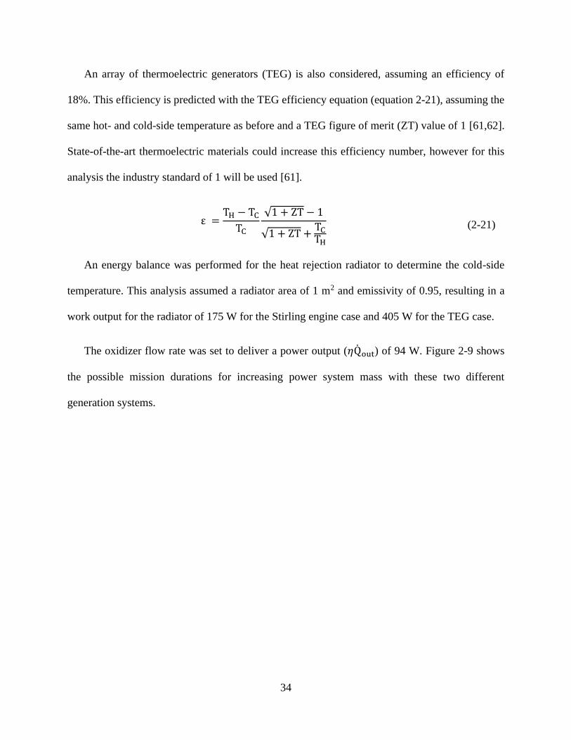
Figure 2-9: Mission duration versus reactants mass for 94 W lander........................................... 35
Figure 3-1: ARL Li-SF6 reactor vessel ......................................................................................... 44
Figure 3-2: Li-CO2 reactor vessel R1.0 ........................................................................................ 44
Figure 3-3: Process and instrumentation diagram (R1.0): heat delivery to coolant air via
immersed heat exchanger coil ....................................................................................................... 45
Figure 3-4: Process and instrumentation diagram (R3.0-R3.2): heat delivery through copper bar
to water-cooled heat sink .............................................................................................................. 47
Figure 3-5: Software user interface (version R1.0) ...................................................................... 48
Figure 3-6: Front view of Li-CO2 reactor test stand, b. Rear view of test stand (with water-cooled
copper conductor heat delivery).................................................................................................... 49
ix
Figure 3-7: R1.0 batch reactor ...................................................................................................... 52
Figure 3-8: a) Temperature measurements from different depths in reactor R1.0, b) Coolant inlet
and outlet temperatures and corresponding instantaneous heat delivery rate (uncertainty in
temperature ± 2.2°C, heat rate ± 4 W) .......................................................................................... 53
Figure 3-9: Reactor 1.0 CT scan cross-section ............................................................................. 54
Figure 3-10: Photograph of reactor 2.0, red lines indicate approximate depths of the three
injectors ......................................................................................................................................... 56
Figure 3-11: Post-test CT-scan cross-sections of Reactor 2.0, indicating blockages in the injector
tubes .............................................................................................................................................. 58
Figure 3-12: Rendering of reactor assembly with copper conducting collar and water-cooled heat
sink ................................................................................................................................................ 59
Figure 3-13: a) Reactor 3.0 bath thermocouple probe traces, b) Reactor 3.0 oxidizer flow rate and
verage heat delivery rate measured through the copper conductor (uncertainty in temperature ±
2.2°C, heat rate ± 1 W, flow rate ± 0.1 SLM)............................................................................... 61
Figure 3-14: a) R3.1 with stainless steel shield and wire mesh installed, b) drawing of the shield
before it was rolled and welded (right) ......................................................................................... 62
Figure 3-15: a) Reactor 3.1 bath thermocouple probe traces, b. Reactor 3.1 oxidizer flow rate and
average heat delivery rate measured through the copper conductor assembly (uncertainty in
temperature ± 2.2°C, heat rate ± 1 W, flow rate ± 0.1 SLM)) ...................................................... 63
Figure 3-16: a) Reactor 3.1 bath thermocouple probe traces, b) Reactor 3.1 oxidizer flow rate and
average heat delivery rate measured through the copper conductor (uncertainty in temperature ±
2.2°C, heat rate ± 2 W, flow rate ± 0.1 SLM)............................................................................... 64

x
Figure 3-17: Cross-section CT scan images for reactors. Green dashed lines show separation of
products from air (above) and presumed metallic lithium (below). Red solid and dashed lines
show locations of the SS shield and wick, respectively, in R3.1. ................................................. 66
Figure 3-18: Schematic of procedure to estimate unreacted lithium volume (Reactor 3.0). Step 1:
Import CT scan data into ParaView. Step 2: Trim data to only include reactor interior. Step 3:
Determine horizontal plane below which unreacted lithium is present (image sliced in half to
view interior). Step 4: Apply threshold intensity cutoff to isolate unreacted lithium and calculate
the volume. .................................................................................................................................... 67
Figure 4-1: Rankine cycle diagram ............................................................................................... 79
Figure 4-2: Venus surface model, T-s diagram ............................................................................ 80
Figure 4-3: Venus surface model, P-h diagram ............................................................................ 80
Figure 4-4: Lab scaled model, T-s diagram .................................................................................. 82
Figure 4-5: Lab scaled model, P-h diagram .................................................................................. 82
Figure 5-1: Complete mercury vapor Rankine cycle test stand with main components highlighted
....................................................................................................................................................... 87
Figure 5-2: Plumbing and Instrumentation Diagram (P&ID) for experimental facility ............... 88
Figure 5-3: Satellite control box ................................................................................................... 89
Figure 5-4: LabVIEW user interface ............................................................................................ 90
Figure 5-5: SolidWorks rendering of the evaporator design ........................................................ 91
Figure 5-6: SolidWorks model of tube-in-tube condenser ........................................................... 92
Figure 5-7: Aluminum, water-cooled enclosure for pump and flow meter .................................. 94
Figure 5-8: Liquid mercury reservoir on test stand (left) and diagram of conductivity sensors
(right) ............................................................................................................................................ 95
xi
Figure 5-9: Turbine magnetically coupled with DC motor .......................................................... 96
Figure 5-10: Cold trap with Peltier cooler for mercury removal .................................................. 97
Figure 5-11: Cordier diagram for turbines .................................................................................... 99
Figure 5-12: Rotary vane expander cross-sectional diagram [110] ............................................ 100
Figure 5-13: RVE version 1, SolidWorks assembly ................................................................... 101
Figure 5-14: RVE SolidWorks drawing ..................................................................................... 102
Figure 5-15: RVE version 2, SolidWorks assembly (left) and installed on test stand (right) .... 102
Figure 5-16: RVE torque vs RPM graph comparing the two versions ....................................... 103
Figure 5-17: RVE vanes before and after testing. Graphite (left), hBN (middle), hBN-AlN (right)
..................................................................................................................................................... 104
Figure 5-18: RVE ceramic chamber prototype, exploded SolidWorks view ............................. 105
Figure 5-19: RVE ceramic chamber ........................................................................................... 106
xii
LIST OF TABLES Table 2-1: ALIVE Mission Parameters ........................................................................................ 18
Table 2-2: Dimensions for baseline conditions ............................................................................ 23
Table 3-1: Summary of reactor tests and their respective features ............................................... 51
Table 3-2: Summary of reaction data from tests, with ranges of: yields for reactions 1-2 and 1-3
(f2, f3), final overall composition, and effective specific energies on total fuel and reacted fuel
bases (based on energy balance calculation) ................................................................................ 70
Table 4-1: Recuperated Brayton cycle comparison for multiple working fluids.......................... 76
Table 4-2: Rankine cycle inputs and parameters .......................................................................... 78
Table 4-3: Thermodynamic state points for Venus surface model ............................................... 80
Table 4-4: Thermodynamic state points for lab scaled model ...................................................... 81
Table 5-1: Operating conditions and requirements from Section 4.2.2 analysis .......................... 90
Table 5-2: Condenser dimensions and properties for the oil cooling loop and mercury working
fluid ............................................................................................................................................... 93
Table A-1: Summary instrumentation accuracy ......................................................................... 128
Table A-2: Summary of propagated uncertainties ...................................................................... 130
xiii
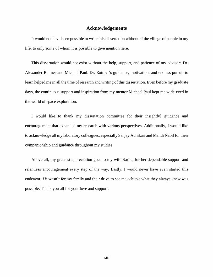
Acknowledgements
It would not have been possible to write this dissertation without of the village of people in my
life, to only some of whom it is possible to give mention here.
This dissertation would not exist without the help, support, and patience of my advisors Dr.
Alexander Rattner and Michael Paul. Dr. Rattner’s guidance, motivation, and endless pursuit to
learn helped me in all the time of research and writing of this dissertation. Even before my graduate
days, the continuous support and inspiration from my mentor Michael Paul kept me wide-eyed in
the world of space exploration.
I would like to thank my dissertation committee for their insightful guidance and
encouragement that expanded my research with various perspectives. Additionally, I would like
to acknowledge all my laboratory colleagues, especially Sanjay Adhikari and Mahdi Nabil for their
companionship and guidance throughout my studies.
Above all, my greatest appreciation goes to my wife Sarita, for her dependable support and
relentless encouragement every step of the way. Lastly, I would never have even started this
endeavor if it wasn’t for my family and their drive to see me achieve what they always knew was
possible. Thank you all for your love and support.
xiv
This dissertation is based upon work partially funded by the United States National
Aeronautics and Space Administration under the NIAC grant number NNX15AQ30G and
HOTTECH award number 80NSSC17K0591. This report was prepared as an account of work
sponsored by an agency of the United States Government. Neither the United States Government
nor any agency thereof, nor any of their employees, makes any warranty, express or implied, or
assumes any legal liability or responsibility for the accuracy, completeness, or usefulness of any
information, apparatus, product, or process disclosed, or represents that its use would not infringe
privately owned rights. References herein to any specific commercial product, process, or service-
water by trade name, trademark, manufacturer, or otherwise does not necessarily constitute or
imply its endorsement, recommendation, or favoring by the United States Government or any
agency thereof. The views and opinions of authors expressed herein do not necessarily state or
reflect those of the United States Government or any agency thereof.

Chapter 1
Introduction and Literature Review
2
Studies of both Venus [1] and Europa surface mission concepts [2,3] and the National Research
Council’s Decadal Survey [4] have identified the scientific value for landing on the surface of
these bodies. However, the extreme environments and low solar availability on the surfaces of
these bodies impose power and thermal management challenges for future missions.
1.1. Extreme environment power and cooling challenges
The opacity of the Venus atmosphere and Europa’s distance from the Sun prevent the use of
solar photovoltaic generators to deliver the desired power range of up to hundreds of Watts [5].
Because of this low solar availability, stored energy sources are necessary to power surface landers
[6]. While electrochemical batteries represent a mature power system option, they significantly
limit mission scope. The longest duration mission on the Venus surface was Venera 13, at just
over two hours. This time constraint was due to reliance on battery power and limited cooling
capacity. Enough batteries could not be transported to provide the spacecraft active cooling to
extend its duration. A mission concept for a Europa lander proposed a battery power source for a
mission duration of twenty days [2,7]. This small lander requires active heating and enough power
to operate and survive the low temperature on the surface of Europa (100 K). Battery powered
missions limit the mission duration and ability to survive the extreme environments on either
target’s surface.
Therefore, extended mission duration concepts have focused on using radioisotope thermal
generators (RTG) power plants. Due to the RTG’s dependency on plutonium 238, an RTG
powered mission effectively requires a New Frontiers ($600M – $1B) or Flagship-class ($2B+)
mission budget. Low cost, power, and mass radioisotope power systems (RPS) have been proposed
to meet this need, but have not yet been demonstrated and would only be available for highest
3
priority missions due to low domestic plutonium supply [8]. Recently, metal-fueled, combustion-
based power plants have been proposed as low-cost alternatives for extended duration missions
[6]. On many planetary bodies, the atmosphere could be used as an in-situ oxidizer for reactive
metal fuels (e.g., CO2 on Venus or Mars), significantly reducing carried mass requirements. The
main benefit of a metal combustion-based power plant is the potential for more than three times
greater system specific energy when compared with the highest performance electrochemical
batteries, such as sodium-sulfur batteries for a Venus mission [6]. Detailed surveys of available
power systems and the benefits for metal combustion-based power plants have been performed
[6,9]. Figure 1-1 shows a qualitative thermal specific energy and specific power comparison for
batteries, chemical storage, RPS, and solar power sources (Ragone plot). RPS and solar power
have very long-life spans and therefore extremely high specific energy. However, RPS isotopes
have low specific power (~500 Wth kg-1) and solar arrays could only produce 8.7-22.0 W m-2 on
the Venus surface [5]. Batteries have a greater specific power potential, but a much lower specific
energy. This suggests that for a Venus mission with a power requirement of hundreds of watts,
chemical storage has a greater potential.
4
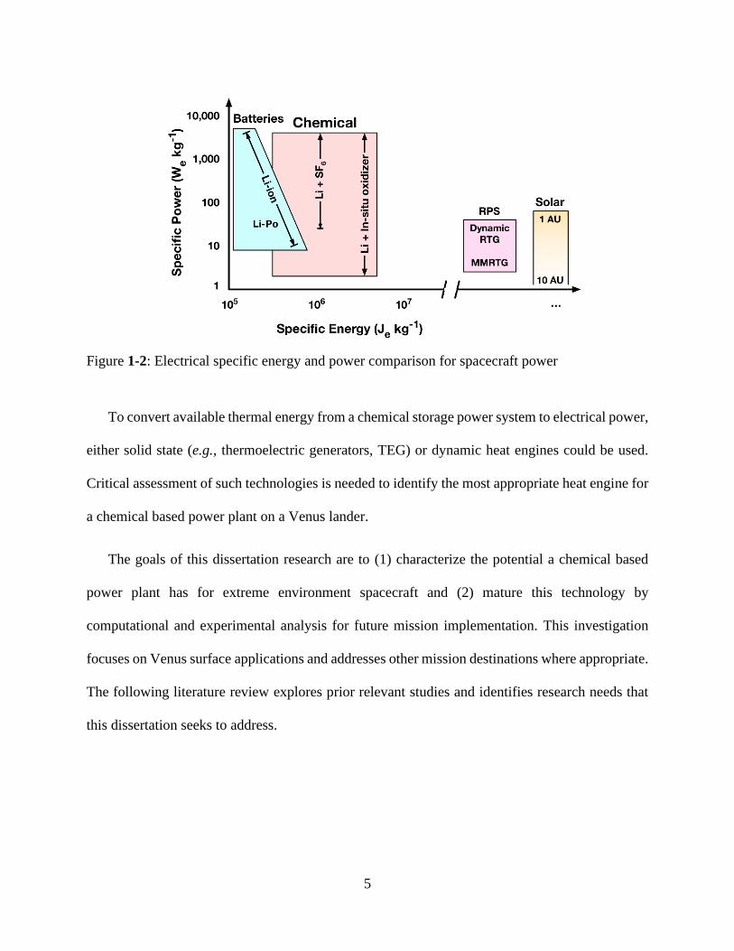
Figure 1-1: Thermal specific energy and power comparison for spacecraft power
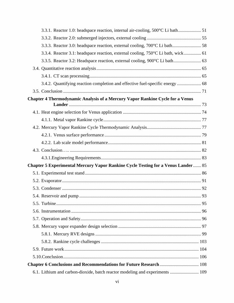
With the greater thermal power however, conversion to electrical power is still required. Figure
1-2 shows the same plot as Figure 1-1, with a conversion to electrical specific energy and power.
For an in-situ Venus lander, the chemical power system has strong potential. However, detailed
analysis of the heat transfer processes to deliver energy from such reactors to potential heat engines
has not yet been performed.
5
Figure 1-2: Electrical specific energy and power comparison for spacecraft power
To convert available thermal energy from a chemical storage power system to electrical power,
either solid state (e.g., thermoelectric generators, TEG) or dynamic heat engines could be used.
Critical assessment of such technologies is needed to identify the most appropriate heat engine for
a chemical based power plant on a Venus lander.
The goals of this dissertation research are to (1) characterize the potential a chemical based
power plant has for extreme environment spacecraft and (2) mature this technology by
computational and experimental analysis for future mission implementation. This investigation
focuses on Venus surface applications and addresses other mission destinations where appropriate.
The following literature review explores prior relevant studies and identifies research needs that
this dissertation seeks to address.
6
1.2. Literature review
1.2.1. Venus surface lander concept
The 2013-2022 planetary decadal survey recommended a Venus In-Situ Explorer (VISE) for
development during 2013–2023 [4]. The Venus Exploration Analysis Group (VEXAG) identified
high priority science objectives of studying the evolution of the surface and interior of Venus,
characterizing interior–surface–atmosphere interactions over time, and determining whether liquid
water was ever present [10]. To accomplish these objectives, data characterizing noble gas
abundances, isotopic ratios, seismic activity, and atmospheric D/H (deuterium and hydrogen)
composition at the surface are required [11]. This will need to be collected over longer periods of
time than any lander has yet survived [1,12–15].
In 1961, the Soviet space program initiated an extensive program of Venus exploration that
included atmospheric probes, landers, orbiters, and balloon missions [16]. This program produced
many successful missions after years of study to determine how to survive and conduct
experiments in the Venus environment. In the late 1970s, NASA conducted a multi-probe program
aimed at characterizing the atmosphere: Pioneer Venus [17]. However, few missions reached the
surface of Venus, and those that did, only collected data for timescales of hours. These landers
used thermal storage phase change materials (PCMs) and multi-layered insulation (MLI) to protect
payloads from rapidly overheating [1,18]. To survive on the surface of Venus (~470°C) for more
than a few hours, active refrigeration may be needed [1,15,19–22]. High-temperature electronics
are in development, but do not currently exist for Venus conditions. Modeling studies suggest that
payloads can be maintained at 25-100°C with 100-360 Wth of refrigeration capacity [12,14,15,23].
This will require power systems with greater energy densities (>200 Wh kg-1) and power levels (>
100s W) than previously fielded [10].
7
To meet this power need for active cooling, radioisotope and chemical heat sources (1.8 - 14
kWth output) have been suggested to drive power generation and refrigeration systems
[12,14,15,19,24,25]. Solutions based on radioisotope power systems (RPS) have been proposed,
but have not yet been demonstrated, and may only be available for the highest priority missions
due to limited supply of 238Pu [8]. Lithium-combustion power systems have been proposed as low-
cost alternatives, which would react stored lithium fuel with ambient atmosphere (96.5% CO2,
3.5% N2) oxidizer (in-situ reactant use, ISRU) [6,9,15]. A study assessing a lithium-ISRU driven
power plant indicated potential for system specific energy of 1.1 kWe -hr kg-1, ~4× the value for
NaS batteries [6]. In the Advanced Long-Life Lander Investigating the Venus Environment
(ALIVE) mission study, a Stirling duplex heat engine and refrigeration system was proposed that
would be powered by lithium combustion with the Venus atmosphere, providing 500 W of power
and 1500 W of cooling for a 120 hr mission [15].
Alternatively, solar power and fuel cell technology have been proposed for aerial and lander
missions but have large challenges to overcome for surface operations due to the extremely low
solar intensity at the surface (<5 W m-2) and very high ambient temperatures (470°C). Solar
photovoltaic technology is being developed, but quantitative projections of specific power have
not been reported [26–28]. Solid oxide fuel cells have been proposed and are being developed for
aerial missions, but have not been analyzed for surface missions to my knowledge [29,30].
Therefore, a proposed scheme for a Venus lithium reactor is as follows. Solid lithium fuel is
stored in a batch reactor vessel. The surface temperature of Venus is about 470°C; at this
temperature, solid lithium fuel melts and become volatile. High-pressure atmosphere is fed into
the reactor as oxidizer, and combustion initiates spontaneously over the surface of the lithium bath.
Experimental studies show combustion can be achieved when a lithium bath is brought to auto-
8
ignition temperatures for the specific oxidizer [9,31–33]. The reaction rate could then be simply
controlled with a valve that modulates the oxidizer flow rate. Oxidizer could be supplied to the
head space over the liquid lithium bath or injected directly into the lithium bath itself. The
postulated combustion process should yield only condensed phase products that are denser than
the lithium bath. In prior comparable lithium-sulfur-hexafluoride combustion systems, these
combustion products sank to the bottom of the reactor vessel, resulting in a constantly refreshing
combustion surface [31]. Because the products are only in a condensed phase, there is no pressure
build up in the reactor and no need for an exhaust. This same behavior is expected for lithium and
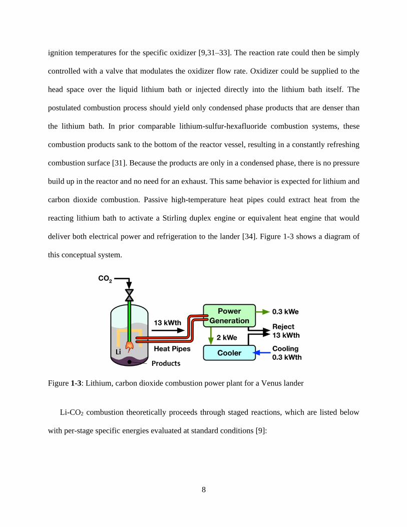
carbon dioxide combustion. Passive high-temperature heat pipes could extract heat from the
reacting lithium bath to activate a Stirling duplex engine or equivalent heat engine that would
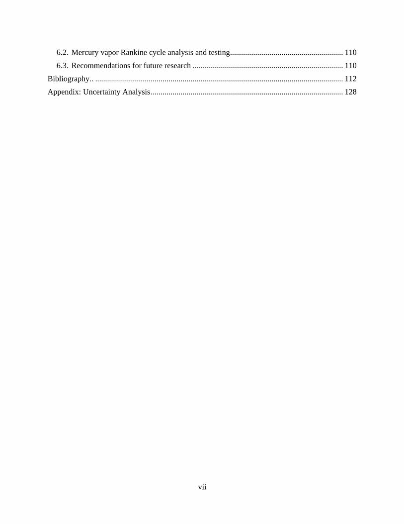
deliver both electrical power and refrigeration to the lander [34]. Figure 1-3 shows a diagram of
this conceptual system.
Figure 1-3: Lithium, carbon dioxide combustion power plant for a Venus lander
Li-CO2 combustion theoretically proceeds through staged reactions, which are listed below
with per-stage specific energies evaluated at standard conditions [9]:
9
5Li + CO2 → 2Li2O + 0.5Li2C2
24.0 MJ kgLi−1 (6.7 kWh kgLi
−1)
18.9 MJ kgCO2
−1 (5.2 kWh kgCO2
−1 )
(1-1)
2Li2C2 + 3CO2 → 2Li2CO3 + 5C + Heat 8.6 MJ kgCO2
−1 (2.4 kWh kgCO2
−1 ) (1-2)
Li2O + CO2 → Li2CO3 + Heat 5.1 MJ kgCO2
−1 (1.4 kWh kgCO2
−1 ) (1-3)
The overall ideal reaction can therefore be defined as follows, with the potential to deliver up
to 45.1 MJth per kg of Li fuel if all stages are completed.
4Li + 3CO2 → 2Li2CO3 + C
45.1 MJ kgLi−1 (12.5 kWh kgLi
−1)
9.5 MJ kgCO2
−1 (2.6 kWh kgCO2
−1 )
(1-4)
This batch reactor concept is attractive because of its simplicity but introduces the risk that
products could freeze and isolate pockets of fuel, reducing effective fuel-specific energy.
Intermediate reaction products may distribute non-uniformly, leading to varying degrees of
completion throughout reactors. Depending on how many of these stages complete, the theoretical
specific energy would range over 24-45 MJ kgLi-1. The ALIVE mission study assumed a
conservative fuel-specific energy of 27.5 MJ kgLi−1 [15]. However, it is unclear what reaction yields
can be realized in relevant conditions. Further experimental investigations are needed to determine
the practical yields and specific energies for lithium batch reactors.
1.2.2. Europa lander concept
While the primarily carbon dioxide atmosphere makes Venus a promising candidate for a
lithium combustion reactor, the technology can be configured for a variety of missions. For a

10
mission to the vacuum environment on the surface of Europa, a lithium and sulfur hexafluoride
combustion power system is proposed. The sulfur hexafluoride oxidizer could be carried onboard
and reacted with the lithium fuel. This self-contained power system could enable a mission of the
same duration as the 2016 lander concept with additional benefits [2]. The high potential power
output would allow a lander to carry previously unconsidered instrumentation, such as a large drill
to penetrate surface ice. A lithium combustion reactor could also warm lander hardware to required
operating temperatures and melt or evaporate surface ice for analysis.
More information can be found for lithium and sulfur-hexafluoride combustion than for carbon
dioxide [6,9,31,33]. Lithium and sulfur hexafluoride combustion technology was developed to
deliver high-power (0.5-1.15 MW) and low power (3-25 kW) to undersea vehicles [31]. This
research showed the high energy density of this technology and its ability for long-term storage
before delivering power on-demand. Lithium and sulfur hexafluoride combustion is known to react
as shown in equation (1-5) with a specific energy of 14.1 MJ kgreactants-1.
8Li + SF6
→ 6LiF + Li2S + Heat (1-5)
Proposed operation is similar to the Venus lander power system concept. However, the oxidizer
would be stored onboard the spacecraft and there would be no refrigeration system. The surface
temperature of Europa is about 100 K, at this temperature the solid lithium fuel would need to be
melted via onboard heaters to a liquid state [3]. Once melted, onboard sulfur-hexafluoride can be
drawn into the reactor and combusted with the lithium fuel. The denser combustion products
should sink to the bottom of the reactor vessel, resulting in a constantly refreshing combustion
surface with no pressure build up and no need for an exhaust. Passive high-temperature heat pipes
could extract heat from the reacting lithium bath activating a heat engine that would deliver
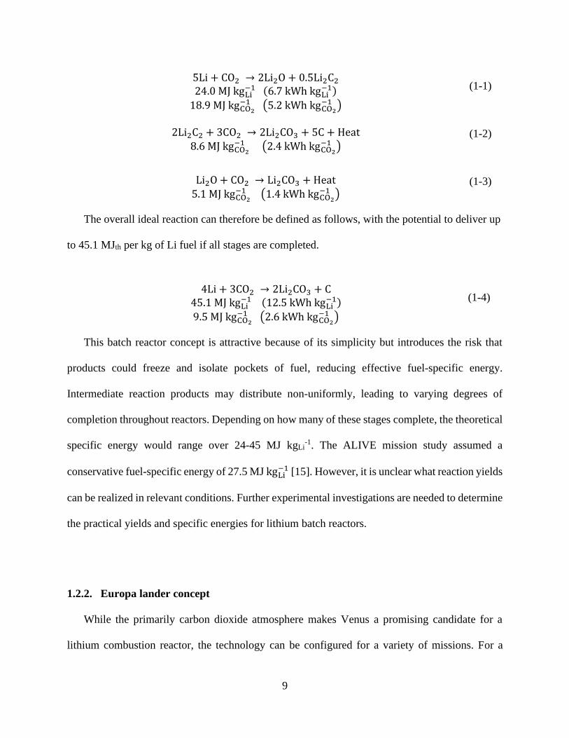
electrical power to the lander. Figure 1-4 shows a diagram of this conceptual system.
11
Figure 1-4: Lithium, sulfur hexafluoride combustion power plant for a Europa lander
1.2.3. Potential in-situ lithium combustion with the Martian atmosphere
Similar to Venus, the Martian atmosphere is comprised of 95% CO2. This allows for potential
in-situ resource utilization that could enable a future sample return or aerial mission as outlined in
the Decadal Survey [4]. Rocket propulsion using the atmospheric CO2 as an oxidizer and on-board
metal fuels have been investigated [35,36]. Magnesium, lithium, and alloys based on these two
metals have been found as the ideal fuels for CO2 combustion due to their spontaneous ignition at
lower temperatures than other fuels [37,38]. Magnesium combustion with CO2 has been well
studied. However, for elemental lithium fuel, only one known experimental combustion study has
been performed for this configuration [37]. That combustion demonstration was successful, but no
known follow-up research and development has been performed. Although the carbon dioxide is
available on Mars, the low atmospheric pressure (610 Pa) may affect ignition temperatures for in-
situ combustion. Future investigations will be required to determine the potential for lithium and
carbon-dioxide combustion for conditions on Mars.
12
1.2.4. High temperature planetary lander heat engines
To take advantage of the high energy and power density of chemical combustion, a heat engine
that can survive and operate efficiently at Venus conditions will be required. Many different
thermodynamic systems have been proposed and analyzed for Venus surface missions to provide
power and/or cooling, including: Stirling converters, Stirling duplex, Rankine cycles, and cascade
refrigeration cycles [14,15,23,39]. However, none of these systems or their components have been
built or tested for survival at Venus conditions. For a future Venus mission to be able to use a heat
engine, the components and the system as a whole need to be tested successfully at relevant
conditions [40].
Although no heat engines have been tested at Venus conditions, metal combustion fueled heat
engines have been designed and built for undersea vehicles [31]. Prior systems were powered with
lithium and sulfur hexafluoride combustion and have operated for extended periods of time. This
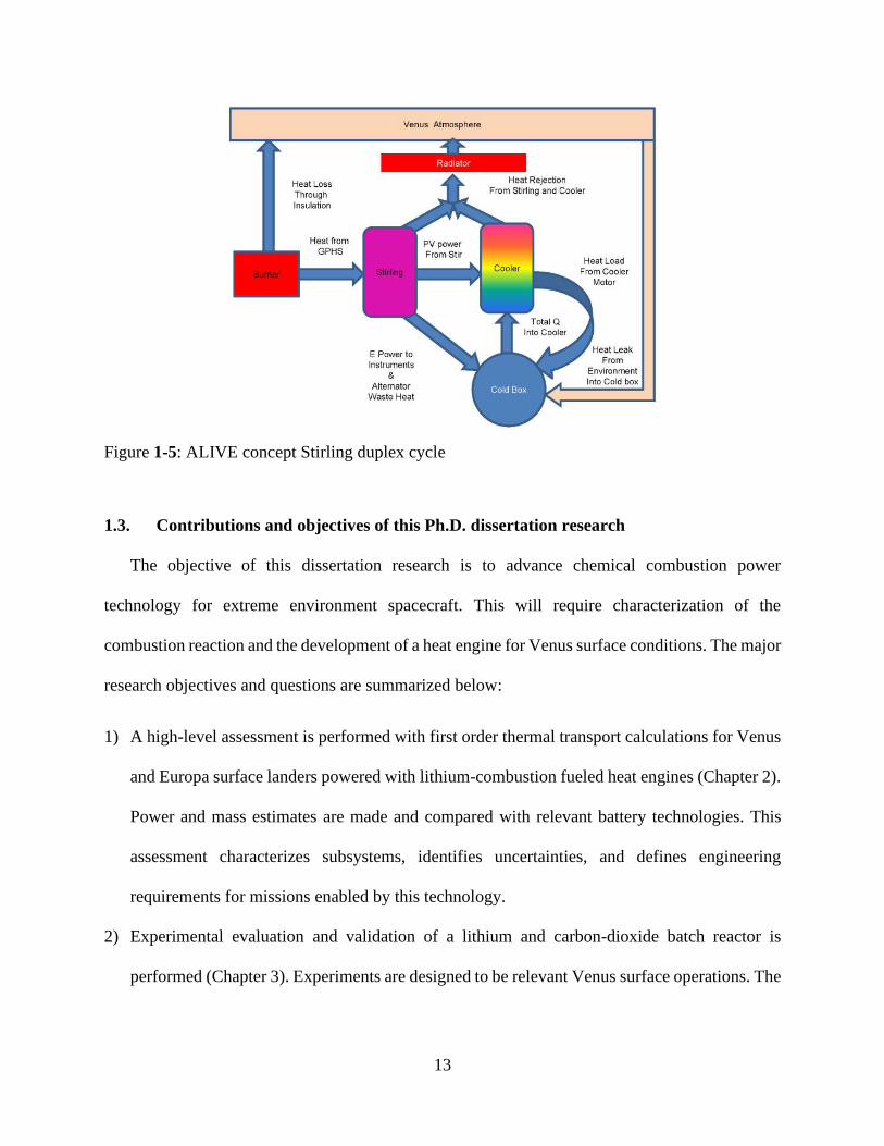
technology is what inspired the ALIVE mission concept design to couple an in-situ lithium
combustor with a Stirling duplex cycle. The Stirling duplex cycle takes the heat from the reaction
and yields mechanical work to provide both electrical power via a generator and cooling to a cold
box via a refrigeration cycle. Figure 1-5 shows an energy transfer diagram of this cycle.
13
Figure 1-5: ALIVE concept Stirling duplex cycle
1.3. Contributions and objectives of this Ph.D. dissertation research
The objective of this dissertation research is to advance chemical combustion power
technology for extreme environment spacecraft. This will require characterization of the
combustion reaction and the development of a heat engine for Venus surface conditions. The major
research objectives and questions are summarized below:
1) A high-level assessment is performed with first order thermal transport calculations for Venus
and Europa surface landers powered with lithium-combustion fueled heat engines (Chapter 2).
Power and mass estimates are made and compared with relevant battery technologies. This
assessment characterizes subsystems, identifies uncertainties, and defines engineering
requirements for missions enabled by this technology.
2) Experimental evaluation and validation of a lithium and carbon-dioxide batch reactor is
performed (Chapter 3). Experiments are designed to be relevant Venus surface operations. The
14
behavior of different reactor configurations, practical utilization of lithium fuel, and specific
energy in batch reactors under varying conditions is analyzed (J kg-1).
3) An analysis and high-level design of a practical Venus surface heat engine is performed
(Chapter 4). Multiple heat engine designs and working fluids are compared, and a promising
candidate technology is identified.
4) A laboratory-scale, proof-of-concept heat engine is designed and the progress on its
construction and development is presented (Chapter 5). Considering the challenge of
replicating and testing at Venusian surface conditions, a step-by-step plan is outlined to mature
this technology.
15
Chapter 2
Analysis of Lithium Combustion Power Systems for
Extreme Environment Spacecraft1
1 Adapted from: C. J. Greer, M. V. Paul, and A. S. Rattner, “Analysis of lithium-combustion power systems for
extreme environment spacecraft,” Acta Astronaut., vol. 151, no. May, pp. 68–79, May 2018.
16
The present investigation develops coupled thermodynamic and heat transfer models for
lithium combustion based power systems for Venus and Europa surface missions. A lithium carbon
dioxide combustion system is evaluated for Venus and a lithium sulfur-hexafluoride system for
Europa. This study analyzes the potential mass savings for lithium combustion power systems
compared with environmentally relevant battery technologies. Subsystems and uncertainties are
identified and characterized, and engineering requirements are defined for missions enabled by
this technology. Future research needs are outlined for the continued maturation of this technology.
A Venus model is presented using a control volume analysis to assess the feasibility of the
proposed ALIVE mission and refine the preliminary analysis performed in the corresponding
report [15] by predicting internal heat transfer processes and heat loss to the ambient. The ALIVE
mission proposed the use of a Stirling duplex engine for energy conversion and cooling. A passive
thermosiphon design delivers heat to a Stirling engine (or comparable heat engine). This study
focuses on combustion and heat transfer analysis within the reactor itself and ignores any potential
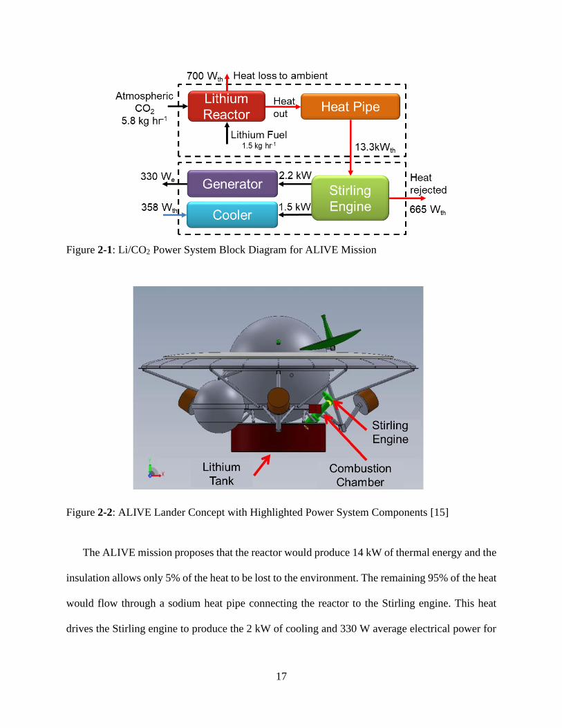
heat loss in the fuel tank. Figure 2-1 shows a block diagram for this ALIVE mission power plant.
Figure 2-2 shows a rendering for this power plant concept with respect to the whole spacecraft
design from the ALIVE mission report.
17
Figure 2-1: Li/CO2 Power System Block Diagram for ALIVE Mission
Figure 2-2: ALIVE Lander Concept with Highlighted Power System Components [15]
The ALIVE mission proposes that the reactor would produce 14 kW of thermal energy and the
insulation allows only 5% of the heat to be lost to the environment. The remaining 95% of the heat
would flow through a sodium heat pipe connecting the reactor to the Stirling engine. This heat
drives the Stirling engine to produce the 2 kW of cooling and 330 W average electrical power for
18
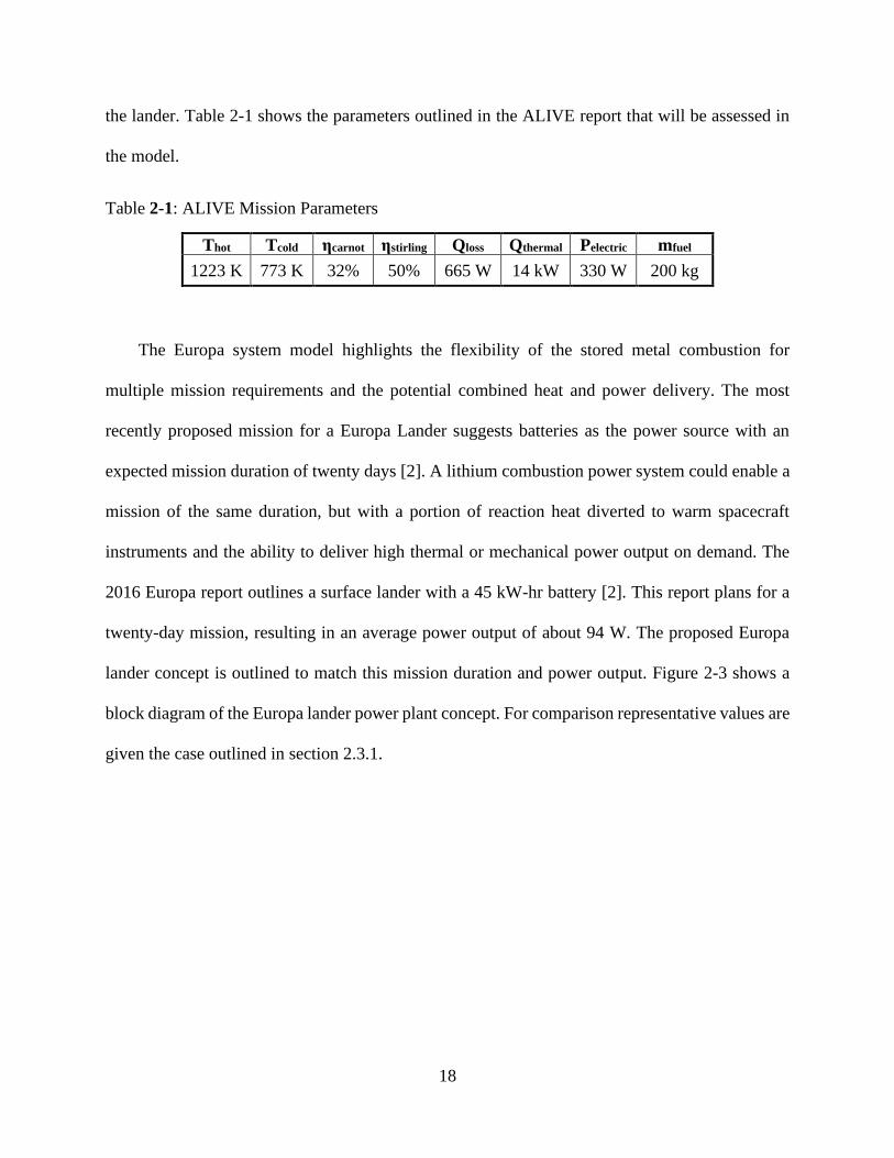
the lander. Table 2-1 shows the parameters outlined in the ALIVE report that will be assessed in
the model.
Table 2-1: ALIVE Mission Parameters
Thot Tcold ηcarnot ηstirling Qloss Qthermal Pelectric mfuel
1223 K 773 K 32% 50% 665 W 14 kW 330 W 200 kg
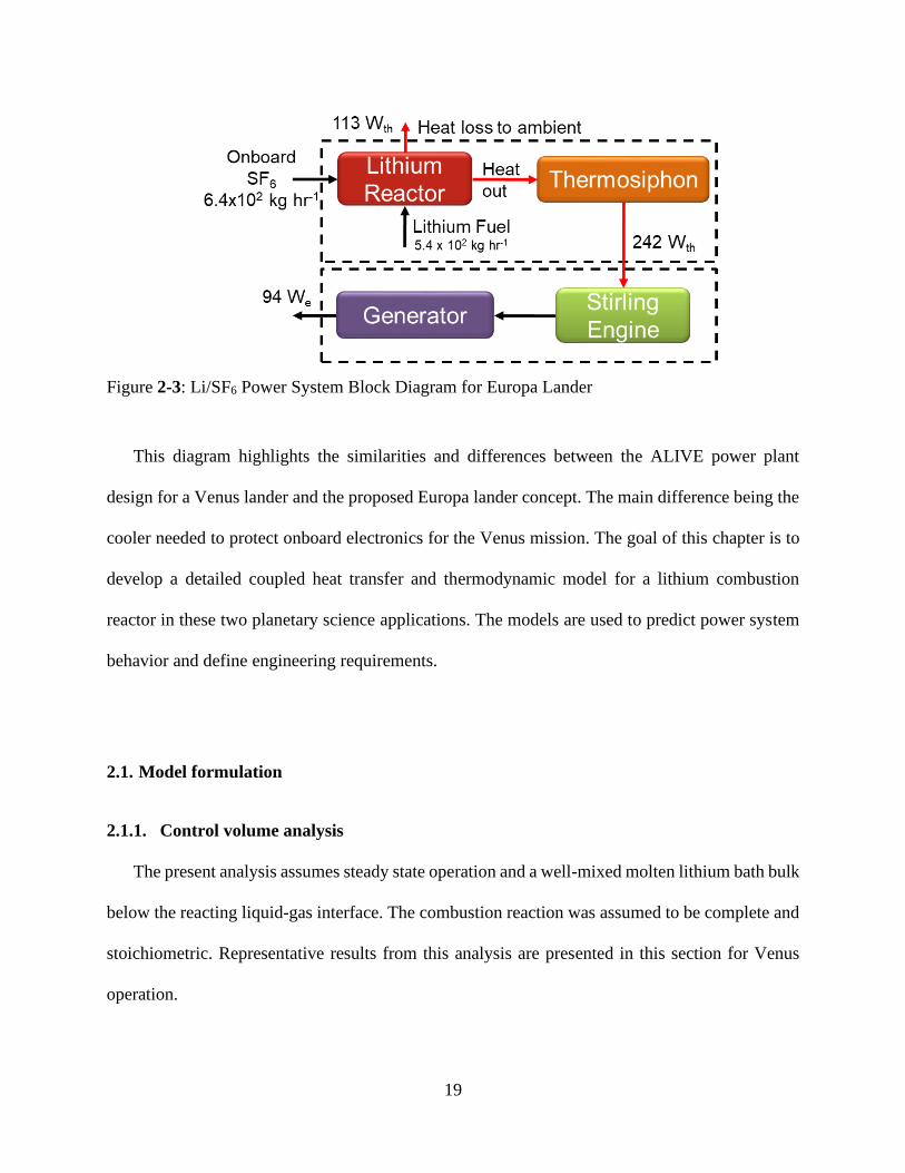
The Europa system model highlights the flexibility of the stored metal combustion for
multiple mission requirements and the potential combined heat and power delivery. The most
recently proposed mission for a Europa Lander suggests batteries as the power source with an
expected mission duration of twenty days [2]. A lithium combustion power system could enable a
mission of the same duration, but with a portion of reaction heat diverted to warm spacecraft
instruments and the ability to deliver high thermal or mechanical power output on demand. The
2016 Europa report outlines a surface lander with a 45 kW-hr battery [2]. This report plans for a
twenty-day mission, resulting in an average power output of about 94 W. The proposed Europa
lander concept is outlined to match this mission duration and power output. Figure 2-3 shows a
block diagram of the Europa lander power plant concept. For comparison representative values are
given the case outlined in section 2.3.1.
19
Figure 2-3: Li/SF6 Power System Block Diagram for Europa Lander
This diagram highlights the similarities and differences between the ALIVE power plant
design for a Venus lander and the proposed Europa lander concept. The main difference being the
cooler needed to protect onboard electronics for the Venus mission. The goal of this chapter is to
develop a detailed coupled heat transfer and thermodynamic model for a lithium combustion
reactor in these two planetary science applications. The models are used to predict power system
behavior and define engineering requirements.
2.1. Model formulation
2.1.1. Control volume analysis
The present analysis assumes steady state operation and a well-mixed molten lithium bath bulk
below the reacting liquid-gas interface. The combustion reaction was assumed to be complete and
stoichiometric. Representative results from this analysis are presented in this section for Venus
operation.
20
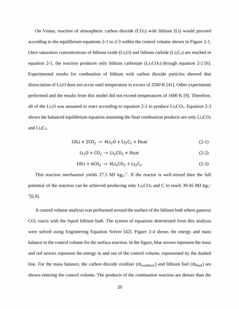
On Venus, reaction of atmospheric carbon dioxide (CO2) with lithium (Li) would proceed
according to the equilibrium equations 2-1 to 2-3 within the control volume shown in Figure 2-1.
Once saturation concentrations of lithium oxide (Li2O) and lithium carbide (Li2C2) are reached in
equation 2-1, the reaction produces only lithium carbonate (Li2CO3) through equation 2-2 [6].
Experimental results for combustion of lithium with carbon dioxide particles showed that
dissociation of Li2O does not occur until temperature in excess of 2500 K [41]. Other experiments
performed and the results from this model did not exceed temperatures of 1600 K [9]. Therefore,
all of the Li2O was assumed to react according to equation 2-2 to produce Li2CO3. Equation 2-3
shows the balanced equilibrium equation assuming the final combustion products are only Li2CO3
and Li2C2.
10Li + 2CO2
→ 4Li2O + Li2C2 + Heat (2-1)
Li2O + CO2
→ Li2CO3 + Heat (2-2)
10Li + 6CO2
→ 4Li2CO3 + Li2C2 (2-3)
This reaction mechanism yields 27.5 MJ kgLi-1. If the reactor is well-mixed then the full
potential of the reaction can be achieved producing only Li2CO3 and C to reach 39-45 MJ kgLi-
1[6,9].
A control volume analysis was performed around the surface of the lithium bath where gaseous
CO2 reacts with the liquid lithium bath. The system of equations determined from this analysis
were solved using Engineering Equation Solver [42]. Figure 2-4 shows the energy and mass
balance in the control volume for the surface reaction. In the figure, blue arrows represent the mass
and red arrows represent the energy in and out of the control volume, represented by the dashed
line. For the mass balance, the carbon dioxide oxidizer (moxidizer) and lithium fuel (mfuel) are
shown entering the control volume. The products of the combustion reaction are denser than the
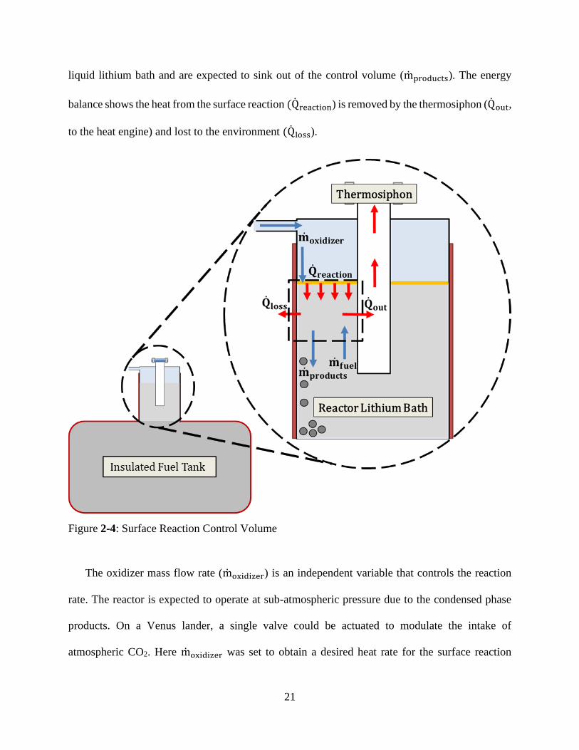
21
liquid lithium bath and are expected to sink out of the control volume (mproducts). The energy
balance shows the heat from the surface reaction (Qreaction) is removed by the thermosiphon (Qout,
to the heat engine) and lost to the environment (Qloss).
Figure 2-4: Surface Reaction Control Volume
The oxidizer mass flow rate (moxidizer) is an independent variable that controls the reaction
rate. The reactor is expected to operate at sub-atmospheric pressure due to the condensed phase
products. On a Venus lander, a single valve could be actuated to modulate the intake of
atmospheric CO2. Here moxidizer was set to obtain a desired heat rate for the surface reaction
22
(Qreaction). The fuel mass flow rate shown in equation 2-4 is a stoichiometric ratio of the oxidizer
flow rate. The products flow rate is the sum of the oxidizer and fuel mass rates as shown in equation
2-5.
mfuel = (10.0
6.0∙
6.9
44.0) ∙ moxidizer (2-4)
mproducts = moxidizer + mfuel (2-5)
With these flow rates, the heat of reaction was determined by balancing the enthalpy (i) of the
reactants and products (equation 2-6).
Qreaction = (moxidizer ∙ ioxidizer) + (mfuel ∙ ifuel) − (mproducts ∙ iproducts) (2-6)
All calculations and fluid properties were obtained using the thermophysical properties library in
EES, NIST JANAF table data, and other sources [42–53].
2.1.2. Baseline condition
The dimensions and design for the reactor model were based on an experimental reactor from
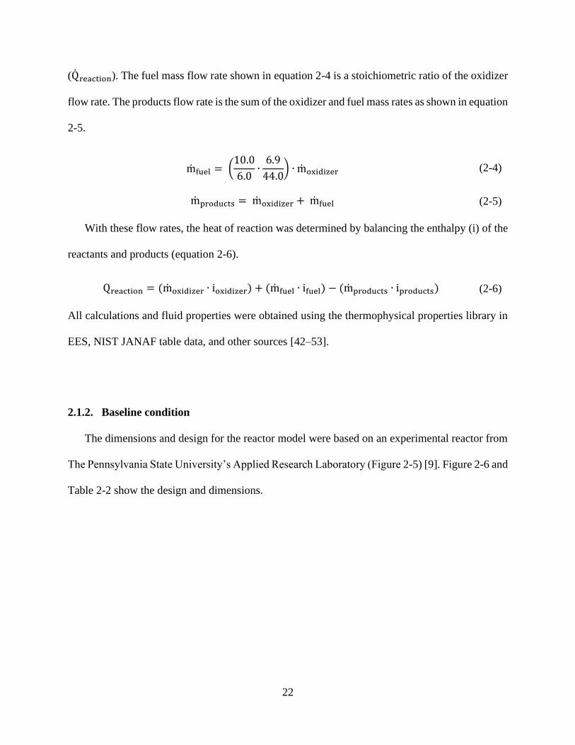
The Pennsylvania State University’s Applied Research Laboratory (Figure 2-5) [9]. Figure 2-6 and
Table 2-2 show the design and dimensions.
23
Table 2-2: Dimensions for baseline conditions
Dimensions Diameter, Dx
(m)
Length, Lx
(m)
Thickness
(m)
Insulation .1654 .4372 .0508
Reactor .1146 .4572 .00602
Thermosiphon .0445 .3429 .00254
Representative predictions for this reactor configuration will be reported in the following
sections of the model development.
2.1.3. Thermal resistance network
A stainless-steel reactor vessel was chosen due to its high melting point and chemical
compatibility with the working fluids. Ceramic fiber insulation around the reactor vessel was
Figure 2-5: Experimental reactor without
insulation
Figure 2-6: Diagram for computational
model
24
chosen due to its high temperature range. For previous missions to Venus multiple insulation
techniques were used, but none were designed to survive the atmospheric conditions for more than
a few hours [54,55]. Materials endurance testing is still needed to determine suitable insulation
materials for long duration Venus missions. The thermosiphon was assumed to be a passive
boiling/condensing heat pipe with a sodium heat transfer fluid. It was assumed to be long enough
to be partially immersed in the lithium bath and transfer almost all the surface reaction heat to the
heat engine.
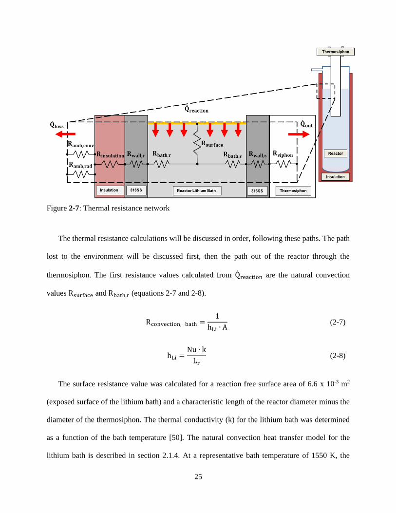
A thermal resistance network model was employed to predict the heat transfer rate from the
surface reaction front to the thermosiphon (Qout) and the heat transfer lost to the ambient (Qloss).
Figure 2-7 shows each resistance stage for the two thermal resistance paths from the reaction front.
The path lost to the ambient (Qloss) starts at the surface reaction, then travels through the lithium
bath, reactor wall, and insulation. Then the heat is radiated and convected to the Venus
environment. The path out of the thermosiphon (Qout) starts at the surface reaction then travels
through the lithium bath, thermosiphon wall, and is then delivered by the boiling sodium pool to
the heat engine hot end.
25
Figure 2-7: Thermal resistance network
The thermal resistance calculations will be discussed in order, following these paths. The path
lost to the environment will be discussed first, then the path out of the reactor through the
thermosiphon. The first resistance values calculated from Qreaction are the natural convection
values Rsurface and Rbath,r (equations 2-7 and 2-8).
Rconvection, bath =1
hLi ∙ A (2-7)
hLi =Nu ∙ k
Lr (2-8)
The surface resistance value was calculated for a reaction free surface area of 6.6 x 10⁻³ m2
(exposed surface of the lithium bath) and a characteristic length of the reactor diameter minus the
diameter of the thermosiphon. The thermal conductivity (k) for the lithium bath was determined
as a function of the bath temperature [50]. The natural convection heat transfer model for the
lithium bath is described in section 2.1.4. At a representative bath temperature of 1550 K, the
26
surface-to-bath natural convection resistance was predicted to be 0.017 K W-1. The thermal
resistance from the lithium bath to the reactor wall followed the same process but for a reactor wall
surface area of 0.17 m2. At a representative bath temperature of 1550 K, the bath-to-wall natural
convection resistance was predicted to be 6.5 x 10⁻⁴ K W-1.
Thermal conduction resistances through the outer reactor vessel wall and insulation were
evaluated with equation 2-9 for conduction through an annulus.
Rconduction =ln (r2 r1)⁄
2π ∙ k ∙ L (2-9)
Based on the reactor dimensions (Table 2-2), the conduction resistance value through the
reactor wall was 1.4 x 10⁻³ K W-1 (assuming k = 28.1 W m-1 K-1 for stainless steel) and 0.81 K W-
1 through the insulation (assuming k = 0.27 W m-1 K-1 for the insulation).
The final two heat loss resistance values are for forced convection and radiation to the ambient.
These resistances are applied in parallel and calculated using equations 2-10 and 2-11.
Rforced convection =D
Nu ∙ k ∙ A (2-10)
Rradiation =(Tinsulation − Tamb)
ε ∙ A ∙ (Tinsulation4 − Tamb
4 ) (2-11)
The convection Nusselt number was determined using the Churchill and Bernstein correlation
(1977) for external flow over a cylinder [56]. The outer diameter of the cylinder was 0.216 m and
the wind speeds for the Venus surface was 2 m s-1. The wind speed value is a conservative
maximum speed based on data from Magellan and the Venera missions [57,58]. Other thermal
properties were determined for a carbon dioxide atmosphere at Venus surface conditions. This
analysis resulted in a Nusselt number of about 1100, a heat transfer coefficient for the reactor
27
insulation to the ambient Venus environment of 275 W m-2 K-1, and a forced convection resistance
value of 0.012 K W-1. This heat transfer coefficient value is within the expected range of 150-1000
W m-2 K-1 from the Venera mission’s data [54]. Radiation thermal resistance was evaluated
assuming a surface emissivity of ε = 0.2 for an oxidized aluminum wrapped vessel [45], resulting
in a thermal resistance value of 0.15 K W-1. The calculated insulation outer surface temperature
was about 750 K with an ambient temperature of 740 K. The total heat loss resistance from the
reacting interface to the Venus environment was found to be 0.82 K W-1, corresponding to a heat
loss rate of 0.7 kW for the baseline operating condition.
Next, the heat delivery flow path through the thermosiphon (Qout) will be followed. The same
natural convection heat transfer model (equation 2-7) is applied between the reaction front and
thermosiphon outer wall. This yielded the same surface-to-bath resistance of 0.17 K W-1 and a
bath-to-wall resistance value of 2.3 x 10⁻³ K W-1 for a thermosiphon area of 0.05 m2. Thermal
conduction through the thermosiphon wall resulted in a resistance of 2.0 x 10⁻³ K W-1.
The convection thermal resistance value through the boiling sodium thermosiphon required
additional analysis, and the detailed formulation is presented in section 2.1.5. For baseline
conditions, a sodium bath temperature of 1223 K resulted in a predicted boiling heat transfer
resistance of 1.8 x 10⁻³ K W-1. All these thermal resistance values were then summed in series. The
total thermal resistance from the reaction front through the thermosiphon was 6.0 x 10⁻³ K W-1,
corresponding to a heat delivery rate of 13.3 kW for the baseline operating condition. With the
total resistance for each path calculated, the heat rates can be calculated as shown in equations 2-
12 to 2-14.
28
Qloss =Tbath − Tamb
Rloss (2-12)
Qout =Tbath − Tsiphon,hot
Rout (2-13)
Qreaction = Qloss + Qout (2-14)
The energy balances, combustion models, and thermal resistance networks were evaluated in
EES. The flow rate of the atmospheric oxidizer was an independent variable and was adjusted to
set system behavior. Findings are detailed in the sections 2.2.1 and 2.2.2 for each target and their
environmental conditions.
2.1.4. Natural convection in a lithium bath
Natural convection heat transfer occurs within the molten lithium bath due to the density
difference between the high temperature fluid at the reaction front (liquid-gas interface) and cooled
fluid near the outer wall and inner thermosiphon. For the baseline geometry, it is expected that a
downward flow pattern would develop along the cooled surfaces of the reactor vessel walls and
on the outside of the thermosiphon wall. In-between these cooled surfaces it is expected that an
upwards flow pattern would occur. No natural convection heat transfer models have been
published for liquid lithium in this specific configuration. As such, the natural convection heat
transfer rates were estimated using results from a related analysis for a cylindrical enclosure with
constant heat flux on the surface and cooling on the side walls [59]. This model defines the Nusselt
number in terms of a modified Boussinesq number (dimensionless natural convection transport
parameter, Bo) accounting for internal heat generation (Bo∗). This correlation is for a modified
Boussinesq number range (4 x 10⁴ < Bo∗ < 2 x 10⁹) as shown in equation 2-15.
29
Nu = 2.9 ∙ Bo∗0.096 (2-15)
The modified Boussinesq number calculation uses a heat flux value that was replaced for this
analysis with the heat of reaction from the surface combustion in the lithium reactor as shown in
equation 2-16. The following fluid properties were calculated for a bath temperature of 1550 K:
thermal expansion coefficient of β = 2.4 x 10⁻⁴ K-1, thermal diffusivity of α = 3.5 x 10⁻⁵ m2 s-1, and
a thermal conductivity of k = 62 W m-1 K-1. This resulted in a modified Boussinesq number of 1.2
x 105. These values were determined using the same sources listed at the end of Section 2.1.1. The
gravitational force was used for Venus of g = 8.87 m s-2, and the characteristic length was set as
the diameter of the reactor minus the diameter of the thermosiphon to 0.63 m.
Bo∗ =g ∙ β ∙ Qreaction ∙ Lr
4
α2 ∙ k (2-16)
The Nusselt number of 8.9 was calculated resulting in a heat transfer coefficient of
8800 W m- 2 K-1 from the reaction front though the lithium bath to the vessel walls. This coefficient
was used in equation 2-7 to find the thermal resistance value for the lithium bath (section 2.1.3).
2.1.5. Sodium pool boiling in the thermosiphon
A two-phase sodium thermosiphon was selected to transfer heat from the lithium pool to the
heat engine. The pool boiling sodium heat transfer correlation [60] was employed as shown in
equation 2-17. This correlation was for heat flux per unit area and was converted from Btu hr-1 ft- 2
with a temperature input of Fahrenheit to Watts with a temperature input of Kelvin. Equation 2-17
was then coupled with equation 2-18 to find the heat transfer coefficient (hsodium).
30
Qout = 57.06 ∙ Asiphon, ∙ (9
5ΔTsat)2.35 (2-17)
Qout = hsodium ∙ Asiphon ∙ (ΔTsat) (2-18)
This heat transfer coefficient was calculated to be 13.2 kW m-2 K-1 for the baseline condition
and was used in equation 2-7 to find the thermal resistance value for the sodium bath (section
2.1.3). This analysis assumed the condenser surface to be large compared to the boiling surface
resulting in a negligible resistance value for the condensation heat transfer to the Stirling engine.
2.2. Data and results
2.2.1. Venus mission with carbon dioxide oxidizer
A model for a Venus lander using the carbon dioxide atmosphere as the oxidizer was evaluated.
The conditions for this test were derived from the ALIVE mission concept [15]. The present model
found that the oxidizer flow rate had to be decreased from 6.3 kg hr-1 (ALIVE mission) to 5.8 kg
hr-1 to obtain a desired reaction heat rate of 14.0 kWth. This discrepancy may be due to a different
heat of reaction found in this model (equation 6) than assumed in the ALIVE report (specific value
not reported in [15]). The hot side of the thermosiphon was set just above the Stirling engine hot
side upper temperature limit of 1223 K [15]. It was found that of the 14 kW of thermal energy,
13.3 kW of heat would be transferred to the thermosiphon and 0.7 kW of heat lost to the
environment, similar to the target 5% heat loss rate from the ALIVE report. The ALIVE mission
predicted a fuel mass of 200 kg to achieve a mission duration of five days. The steady-state oxidizer
flow rate from the model was multiplied by the desired mission duration to obtain the total fuel
mass. If the power system design is similar to the ALIVE mission concept (Figure 2-1), then the
fuel tank can be sized to carry the desired mass for the mission.
31
With a fixed heat rate of 14 kWth, a linear relationship was found between the fuel mass and
mission duration. This relationship showed that for every 50 kg of fuel mass the lander can survive
for 1.36 days. For a mission duration of five days, a fuel mass of about 185 kg was determined.
This value is 13% less than the ALIVE mission’s predicted fuel mass.
An additional analysis was done to determine the relationship between mission duration and
fuel mass for a fixed usable cooling and electrical power of 1 kW. A Stirling engine could use the
reaction heat to deliver both electrical power and refrigeration. Here, useful power output is
estimated with an assumed conversion efficiency (𝑃out = ηQout). A conceptual Stirling engine is
considered with an efficiency of 16%. This efficiency was determined based on a correlation for
the Stirling engine second law efficiency as seen in equation 2-19 [6]. This efficiency was
determined for hot and cold-side temperatures of 1223 K and 740 K, respectively.
ηstirling = 0.3323 (TH
TC)
0.3655
(1 −TC
TH) (2-19)
With a fixed power output of 1kW for this Stirling engine, a linear relationship was found
between the fuel mass and mission duration. This relationship showed that for every 17 kg of fuel
mass the lander can survive for another day. For a five-day mission producing 1 kW of usable
power the Stirling engine would require about 86 kg of fuel mass. The mass of the Stirling engine
power system, fuel tanks, reactor vessel, and additional components was set as 59 kg [6]. This
results in a total power system mass with the Stirling engine for a five-day mission of 145 kg. This
performance with the Stirling engine system can be compared to high performance electrochemical
batteries. Here, a sulfur-sodium battery with a system specific energy of 300 W hr kg-1 was
considered [6]. For a five-day mission duration producing 1 kW of power, 400 kg of battery mass
32
would be required. This is a 176% greater mass requirement than with the presented conceptual
Stirling powered system.
If a longer mission duration is considered, then a Stirling engine power system could power a
ten-day mission with 1 kW of usable power for a total mass of 231 kg. Where the same mission
with sulfur-sodium batteries would require 246% more mass.
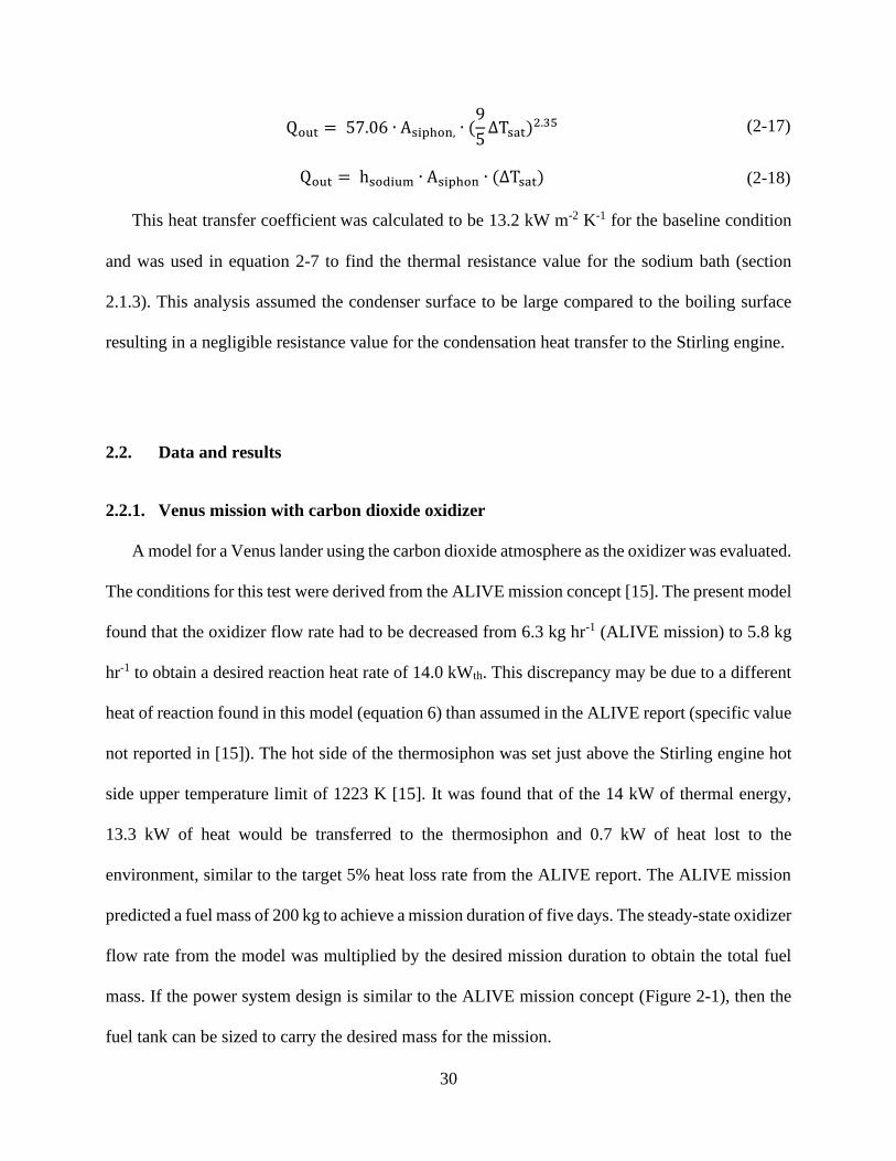
Another analysis was performed to show benefit of variable power with a lithium combustion
power source. Figure 2-8 shows the plot of the possible heat output rate versus the oxidizer flow
rate.
Figure 2-8: Heat rate versus oxidizer flow rate for a fixed fuel mass of 185kg
This shows how the heat of reaction, the heat delivery to the thermosiphon, and the heat lost
to the environment change with increasing oxidizer flow rate. If more power is temporarily
required for a specific instrument (e.g., a drill to collect samples), the oxidizer flow rate could be
increased and later returned to the baseline condition. This flexibility could greatly increase the
scientific instrumentation and mission goals beyond a fixed power output system, such as an RTG.
33
2.2.2. Europa mission with sulfur-hexafluoride oxidizer
A lithium combustion power system with a sulfur-hexafluoride oxidizer can be applied to other
environments where in-situ resource utilization is not possible. The same benefits previously stated
for a Venus lander, apply for a Europa lander. Additionally, a portion of reaction heat could be
directly applied to warm temperature sensitive instruments. One major change to the system is that
the oxidizer will need to be carried by the spacecraft. The balanced combustion reaction for lithium
and sulfur-hexafluoride was assumed complete and stoichiometric as shown in equation 2-20.
8Li + SF6
→ 6LiF + Li2S + Heat (2-20)
This system model followed the same control volume approach described in Section 2.1.1. The
same thermal resistance network from Figure 2-4 was applied for this system; however, there is
no external convection due to the surface of Europa’s lack of atmosphere. Another difference in
the application of a lithium combustion power system for Europa is that the lithium fuel will need
to be heated to a liquid state before combustion can occur. Previous lithium and sulfur-hexafluoride
systems used a pyrotechnic starting charge to melt some of the frozen lithium and initiate the
reaction [31]. For this analysis, it was assumed that the lithium bath is already above its melting
temperature of about 455 K.
The 2016 Europa report outlines a twenty-day mission surface lander with an average power
output of about 94 W [2]. This value was the target range for the Europa model analysis. To achieve
this, two heat engines were considered that could convert the reaction heat to electrical power. A
theoretical Stirling engine is considered here with an efficiency of 39%. This efficiency was
predicted following the same analysis in section 2.2.1 but with hot side and cold-side temperatures
of 700 K and 190 K, respectively.
34
An array of thermoelectric generators (TEG) is also considered, assuming an efficiency of
18%. This efficiency is predicted with the TEG efficiency equation (equation 2-21), assuming the
same hot- and cold-side temperature as before and a TEG figure of merit (ZT) value of 1 [61,62].
State-of-the-art thermoelectric materials could increase this efficiency number, however for this
analysis the industry standard of 1 will be used [61].
ε =TH − TC
TC
√1 + ZT − 1
√1 + ZT +TC
TH
(2-21)
An energy balance was performed for the heat rejection radiator to determine the cold-side
temperature. This analysis assumed a radiator area of 1 m2 and emissivity of 0.95, resulting in a
work output for the radiator of 175 W for the Stirling engine case and 405 W for the TEG case.
The oxidizer flow rate was set to deliver a power output (𝜂Qout) of 94 W. Figure 2-9 shows
the possible mission durations for increasing power system mass with these two different
generation systems.
35
Figure 2-9: Mission duration versus reactants mass for 94 W lander
For a lander with a twenty-day surface mission and a Stirling engine, 94 W of power can be
provided with a reactants mass of about 43 kg (accounting for both lithium fuel and sulfur-
hexafluoride oxidizer). To achieve this, the reactor produced 355 W from the reaction with 113 W
of heat lost to the environment and 242 W of energy out the thermosiphon. This linear relationship
shows that for every 2.15 kg of reactants mass the lander can survive for another day. The mass of
the Stirling engine power system was assumed to be the same as NASA’s advanced Stirling
radioisotope generator of 32 kg [63]. The reactants tanks, reactor vessel, and additional
components are assumed to be an additional 5 kg. This results in a total power system mass for a
94 W, twenty-day mission with the Stirling engine of 80 kg.
With TEGs, a twenty-day mission at 94 W of power would require about 92 kg of reactants
mass. To achieve this, the reactor produced 760 W from the reaction with 115 W of heat lost to
the environment and 645 W of heat out the thermosiphon. This linear relationship shows that for
every 4.57 kg of reactants mass the lander can survive for another day. The mass of the TEG array
is assumed to be 6 kg [64] and the reactants tanks, reactor vessel, and additional components are
36
assumed to be an additional 5 kg. This results in a total power system mass for a 94 W, twenty day
mission with a TEG array of 103 kg.
For comparison, a sulfur-sodium battery with a system specific energy of 300 W hr kg-1 was
assumed, resulting in a required battery mass of 150 kg [6]. This is a total power system mass
increase of about 88% compared to the Stirling engine and 46% compared to the TEG array.
2.2.3. Limitations of proposed model and future research needs
One limitation of this model is that it assumes complete lithium combustion. Previous studies
focused on undersea vehicle power plants and have not required or attempted complete combustion
of all the available lithium fuel. It is not yet known what reaction yields are feasible for alkali metal
combustion in closed reactors.
Another assumption for the combustion was for the reaction to be stoichiometric. Since no
known data is available for complete combustion in a closed reactor, little is known about the final
products of reaction. This model assumed all of the Li2O reacted with available CO2 to form
Li2CO3. These assumptions from the present model result in a heat of reaction at a reference
temperature of 298 K of 34.6 MJ kgLi-1. However, if not all Li2O were converted to Li2CO3, the
following reaction may occur: Li + aCO2 → bLi2O + cLi2C2 + dLi2CO3. If 20% of the supplied
lithium was converted to Li2O, then the resulting heat of reaction at 298 K would be 31.3 MJ kgLi-
1 (-10%). Future experiments are needed to quantify reaction yield and product composition to
enable more accurate prediction of reactor heat output.
Another limitation of this model is that it adapts a natural convection correlation to predict heat
transfer in the lithium bath [59]. The selected correlation was developed for a related, yet distinct,
37
heat transfer configuration for a sodium pool with heating from a nuclear accident. If the actual
natural convection heat transfer coefficients were 50% lower than estimated with this correlation,
the predicted delivered heat for the baseline Venus model case would reduce from 13.3 kW to 12.2
kW (-8%). Experimental or computational investigation of this specific heat transfer configuration
could reduce this component of the model uncertainty.
2.3. Conclusion
Findings were applied to specify engineering requirements for potential lander missions to the
surfaces of Venus and Europa. It was found a lithium combustion power system with an in-situ,
carbon dioxide oxidizer could power a Venus lander with 14 kWth of thermal energy for five days
with 185 kg of fuel. Even greater mission durations are possible if lower power missions are
considered. The potential performances of a Li-CO2 powered Stirling engine and sulfur-sodium
batteries were compared. It was found that sulfur-sodium batteries would require about 176% to
246% more mass to provide 1 kW of power output for mission durations of five to ten days,
respectively.
A lithium combustion power system with a sulfur-hexafluoride oxidizer can provide a Europa
lander with 94 W of power for up to twenty days with 43 kg of reactants mass. A Stirling engine
and TEG array were compared with sulfur-sodium batteries to meet this power and mission
duration requirement. It was found that to provide 94 We power for a twenty-day mission, sulfur-
sodium batteries would require about 46-88% more mass than a TEG array or a Stirling engine
respectively.
Future work includes validating and refining this model with earth-based experimental data
and addressing uncertainties in closure models and assumptions. At the time of writing, no heat
38
transfer data has been reported for the specific configuration of liquid lithium natural convection
in an annulus with top-heating (reaction) and side-cooling (thermosiphon and reactor wall).
Correlations from related studies of sodium natural convection and heat transfer were adopted to
estimate the thermal resistance in this process [59,60]. This model assumed complete and
stoichiometric combustion of lithium and the oxidizer. Future experiments are warranted to
determine feasible reaction yields and product composition. In chapter 3 an experimental facility
is described that was built to measure lithium combustion temperatures and heat flow in order to
answer these questions. Data from these experiments will be applied to assess reaction yield,
stoichiometry of products, and specific energy of the reaction. These results can inform more
mature reactor models and designs to support landed missions to challenging low insolation and
high temperature destinations.
2.3.1. Engineering Requirements
• For a reactor vessel following the Venus baseline condition with two inches of ceramic fiber
insulation, a thermal resistance out of the vessel of 0.82 K W-1 and a resistance out the
thermosiphon of 6.0 x 10⁻³ K W-1 can be expected.
• For the Venus baseline condition, with an oxidizer flow rate of 5.8 kg hr-1, a surface reaction
temperature of 1550 K and an average bath temperature of 1300 K can be expected.
• For a reactor vessel following the Europa baseline condition with two inches of ceramic fiber
insulation, a thermal resistance out of the vessel of 5.4 K W-1 and a resistance out the
thermosiphon of 0.025 K W-1 can be expected.
• For the Europa baseline condition, with an oxidizer flow rate of 0.064 kg hr-1, a surface reaction
temperature of 720 K and an average bath temperature of 705 K can be expected.

39
• UA values for the thermosiphon for both the Venus and Europa cases were found to be 166
W/K and 40 W/K respectively.
• The required lithium fuel tank volume for a 5-day Venus mission and 20-day Europa mission
with a Stirling heat engine would be 0.43 m3 and 0.063 m3 respectively.
40
Chapter 3
Experimental Characterization of Lithium-Carbon
Dioxide Combustion in Batch Reactors for Powering
Venus Landers2
2 Adapted from: Acta Astronautica, https://doi.org/10.1016/j.actaastro.2021.01.010 C. J. Greer, J. A. Peters, M. P.
Manahan, J. J. Cor, and A. S. Rattner, “Experimental characterization of lithium-carbon dioxide combustion in batch
reactorsfor powering Venus landers,” Acta Astronautica, available online Janurary 2021, in press, journal pre-proof.
41
The primary objective of this chapter is to experimentally determine the practical reaction
yields and specific energy levels that can be achieved with Li-CO2 batch reactors in conditions
relevant to Venus surface missions. To design the reactors for these experiments, previous lithium
combustion experiments were analyzed. Lithium and sulfur-hexafluoride (Li-SF6) batch reactor
combustion technology has been developed and fielded in US Navy undersea vehicles, with power
levels ranging from 3 kW to 1.15 MW [31]. This technology has high energy density, the ability
for long-term storage, and reliability for delivering on-demand power. In such Li-SF6 batch
reactors, products are denser than the fuel and are formed above their melting point (~790°C
eutectic). Thus, the products flow to the bottom of reactors, maintaining a nearly uncontaminated
Li-SF6 interface for high yield. The products of Li-CO2 combustion are also theoretically denser
than molten Li. However, Li2C2, Li2O, and carbon will form in solid phase at anticipated reactor
conditions. It is unknown whether the products from Li-CO2 combustion will passively separate
from the reaction interface.
Comparatively limited information is available about characteristics of Li-CO2 reactions.
Experimental studies have been performed to measure fundamental properties of Li-CO2
combustion, including flame speeds and reaction products [41,65,66]. Such tests were performed
at sufficiently small scales such that the reactants could be assumed well mixed. Additional
experimental studies demonstrated that a closed lithium bath will auto-ignite in contact with CO2
gas [9,31–33].
The only large-scale Li-CO2 batch experiments were performed for a proof-of-concept of Li-
ISRU reactions on Venus [9]. That study included both Li-CO2 and Li-CO2-N2 reaction tests, the
latter more closely approximating the Venus atmosphere. Previous experiments indicated an auto-
ignition temperature of 454°C and demonstrated sustained combustion for eight hours. Products
42
were sampled post-test from various locations in the reactors, and compositions were found to vary
significantly spatially. Neither test was run to completion. Therefore, practical specific energy or
final compositions could not be determined. Additionally, reaction heat was not delivered through
a specific pathway as would be needed for a power-system application. That study demonstrated
the viability of the Li-ISRU power system concept, but also raised questions about the system-
level properties of Li-ISRU thermal batch reactors that the present investigation seeks to address.
It is worth noting that although carbon dioxide and nitrogen make up 99.98% of the chemical
composition at the surface of Venus, trace gases have been found to interact with materials exposed
to simulated Venus surface conditions [67]. It is unknown what affect trace gases could have on
the combustion reaction. However, their effect is expected to be minimal considering their low
concentration. Therefore, current experimentation focuses on the characterization of the Li-CO2
reaction as the first step to developing a combustion-based power system. Additionally, nitrogen
in the reaction is expected to restrain the energy release to the first reaction stage (equation 1-1)
unless it is exhausted to the atmosphere when built up in the reactor with a blower or filtered out
at the reactor’s intake [9].
A proposed scheme for a Venus lithium reactor is as follows. Solid lithium fuel is stored in a
batch reactor vessel. The surface temperature of Venus is about 470°C; at this temperature, solid
lithium fuel melts and become volatile. High-pressure atmosphere is fed into the reactor as
oxidizer, and combustion initiates spontaneously over the surface of the lithium bath. The reaction
rate could be controlled by modulating the oxidizer flow. Oxidizer could be supplied to the head
space over the liquid lithium bath or injected directly into the lithium bath itself. All anticipated
reaction products are denser than the fuel and oxidizer; therefore, pressure should not rise in the
reactor, avoiding the need for exhaust or oxidizer compression. The analysis in Chapter 2 identified
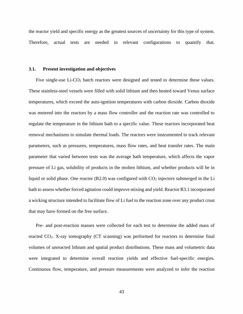
43
the reactor yield and specific energy as the greatest sources of uncertainty for this type of system.
Therefore, actual tests are needed in relevant configurations to quantify that.
3.1. Present investigation and objectives
Five single-use Li-CO2 batch reactors were designed and tested to determine these values.
These stainless-steel vessels were filled with solid lithium and then heated toward Venus surface
temperatures, which exceed the auto-ignition temperatures with carbon dioxide. Carbon dioxide
was metered into the reactors by a mass flow controller and the reaction rate was controlled to
regulate the temperature in the lithium bath to a specific value. These reactors incorporated heat
removal mechanisms to simulate thermal loads. The reactors were instrumented to track relevant
parameters, such as pressures, temperatures, mass flow rates, and heat transfer rates. The main
parameter that varied between tests was the average bath temperature, which affects the vapor
pressure of Li gas, solubility of products in the molten lithium, and whether products will be in
liquid or solid phase. One reactor (R2.0) was configured with CO2 injectors submerged in the Li
bath to assess whether forced agitation could improve mixing and yield. Reactor R3.1 incorporated
a wicking structure intended to facilitate flow of Li fuel to the reaction zone over any product crust
that may have formed on the free surface.
Pre- and post-reaction masses were collected for each test to determine the added mass of
reacted CO2. X-ray tomography (CT scanning) was performed for reactors to determine final
volumes of unreacted lithium and spatial product distributions. These mass and volumetric data
were integrated to determine overall reaction yields and effective fuel-specific energies.
Continuous flow, temperature, and pressure measurements were analyzed to infer the reaction
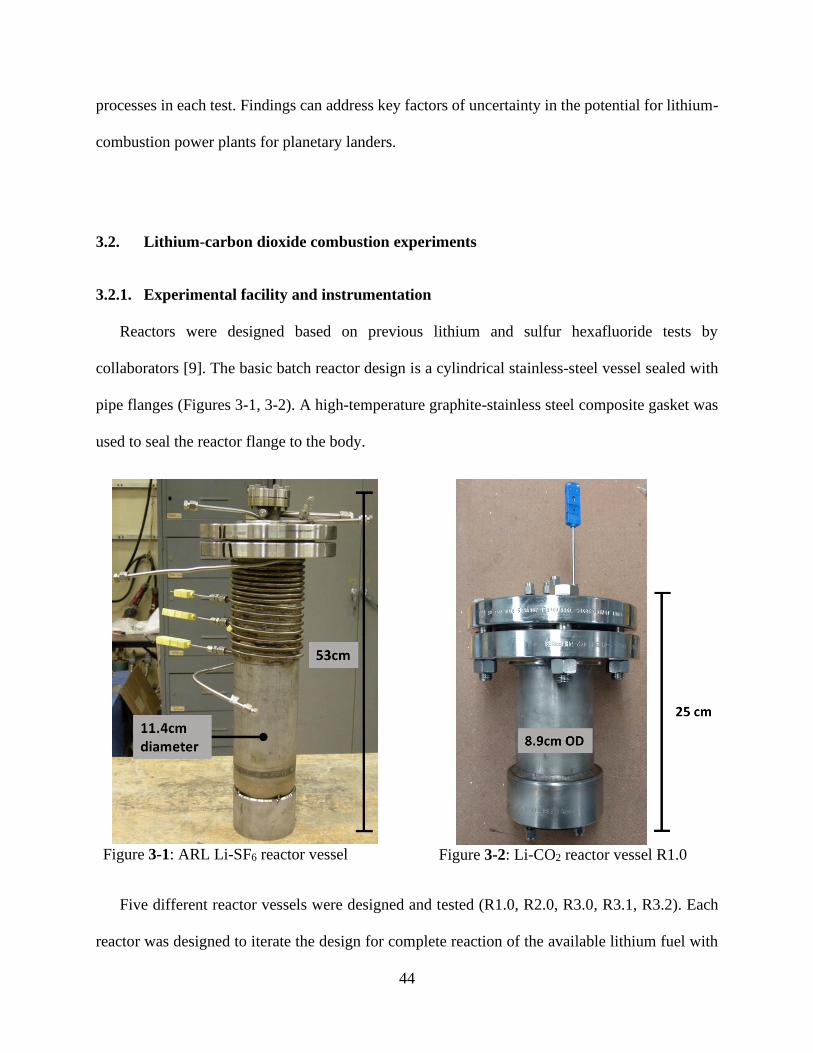
44
processes in each test. Findings can address key factors of uncertainty in the potential for lithium-
combustion power plants for planetary landers.
3.2. Lithium-carbon dioxide combustion experiments
3.2.1. Experimental facility and instrumentation
Reactors were designed based on previous lithium and sulfur hexafluoride tests by
collaborators [9]. The basic batch reactor design is a cylindrical stainless-steel vessel sealed with
pipe flanges (Figures 3-1, 3-2). A high-temperature graphite-stainless steel composite gasket was
used to seal the reactor flange to the body.
Figure 3-1: ARL Li-SF6 reactor vessel
Figure 3-2: Li-CO2 reactor vessel R1.0
Five different reactor vessels were designed and tested (R1.0, R2.0, R3.0, R3.1, R3.2). Each
reactor was designed to iterate the design for complete reaction of the available lithium fuel with
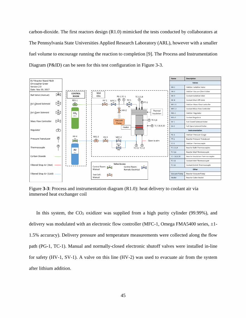
45
carbon-dioxide. The first reactors design (R1.0) mimicked the tests conducted by collaborators at
The Pennsylvania State Universities Applied Research Laboratory (ARL), however with a smaller
fuel volume to encourage running the reaction to completion [9]. The Process and Instrumentation
Diagram (P&ID) can be seen for this test configuration in Figure 3-3.
Figure 3-3: Process and instrumentation diagram (R1.0): heat delivery to coolant air via
immersed heat exchanger coil
In this system, the CO2 oxidizer was supplied from a high purity cylinder (99.99%), and
delivery was modulated with an electronic flow controller (MFC-1, Omega FMA5400 series, ±1-
1.5% accuracy). Delivery pressure and temperature measurements were collected along the flow
path (PG-1, TC-1). Manual and normally-closed electronic shutoff valves were installed in-line
for safety (HV-1, SV-1). A valve on this line (HV-2) was used to evacuate air from the system
after lithium addition.
46
In the first test, compressed air was supplied through a similar flow arrangement to act as a
coolant, simulating a thermal load powered by the reactor. The air acquired reaction heat via a coil
heat exchanger submerged in the molten lithium. Coolant inlet and outlet temperatures were
measured with K-type thermocouples (TC-11,12, ±2.2°C uncertainty) to determine instantaneous
heat delivery rates. In later tests, cooling was provided through a copper conduction bar clamped
to the outside of the reactors (Figure 3-4, Figure 3-12). The free end of the bar was water-cooled,
and its body was thoroughly insulated. A series of thermocouples along the copper bar acted as a
heat-flux sensor.
For the CO2 to auto-ignite with Li, temperatures must be above ~450°C [9]. Therefore, a
resistive heater was installed to preheat the reactors. Thermocouples were installed in each reactor
to record temperatures at multiple points. An absolute pressure transducer (Omega PX119, 0-690
kPa range, ±0.5% accuracy) was used to monitor the pressure inside the reactor vessels. Each
reactor was insulated with mineral wool to limit heat loss to the surroundings.
The test stand was installed in a test cell built for hazardous combustion experiments and was
remotely operated using a software interface and a manual satellite control box. Figure 3-5 shows
the experimental monitoring software and control interface with instrumentation inputs, mass flow
controller output, and the warning indicators for safe maximum temperatures and pressures. The
test stand is shown in Figure 3-6a with an insulated reactor. In Figure 3-6b., the copper-conductor
based cooling system with water-cooling is shown.
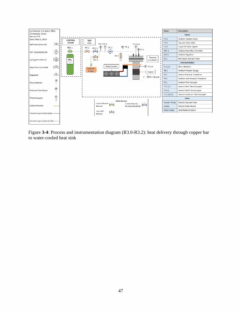
47
Figure 3-4: Process and instrumentation diagram (R3.0-R3.2): heat delivery through copper bar
to water-cooled heat sink
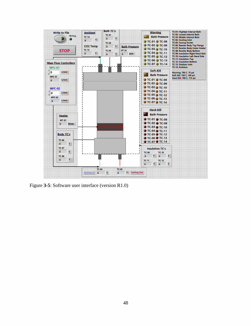
48
Figure 3-5: Software user interface (version R1.0)
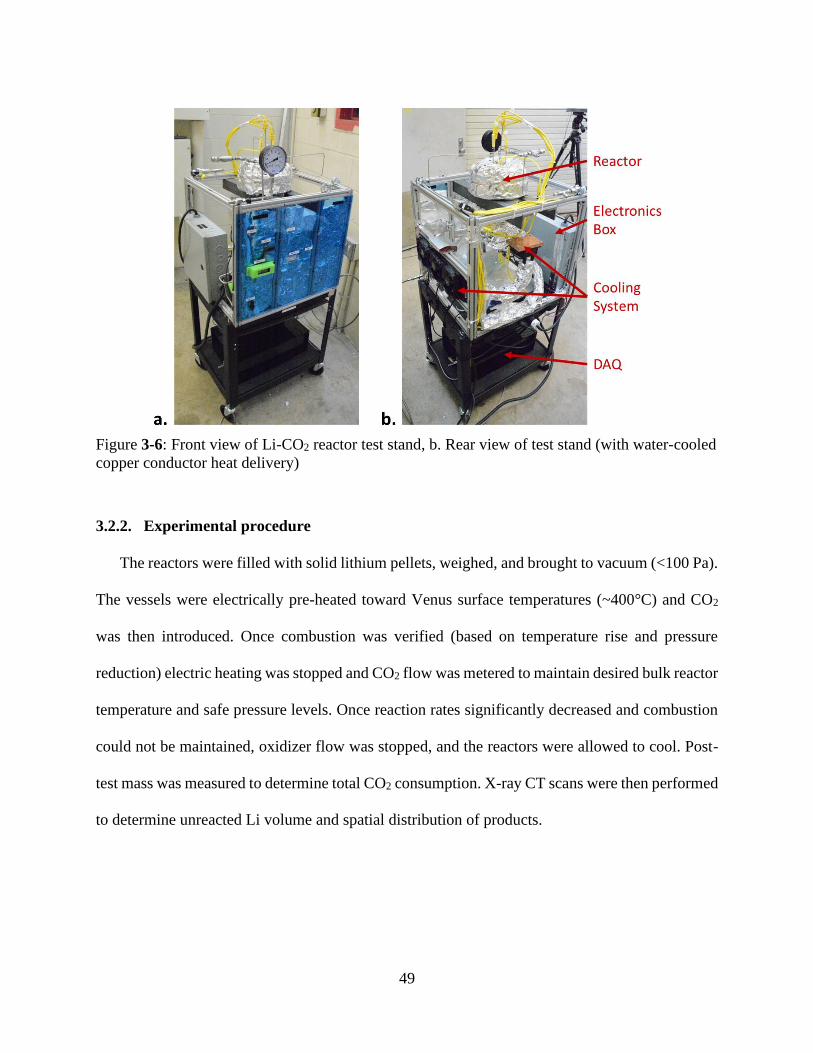
49
Figure 3-6: Front view of Li-CO2 reactor test stand, b. Rear view of test stand (with water-cooled
copper conductor heat delivery)
3.2.2. Experimental procedure
The reactors were filled with solid lithium pellets, weighed, and brought to vacuum (<100 Pa).
The vessels were electrically pre-heated toward Venus surface temperatures (~400°C) and CO2
was then introduced. Once combustion was verified (based on temperature rise and pressure
reduction) electric heating was stopped and CO2 flow was metered to maintain desired bulk reactor
temperature and safe pressure levels. Once reaction rates significantly decreased and combustion
could not be maintained, oxidizer flow was stopped, and the reactors were allowed to cool. Post-
test mass was measured to determine total CO2 consumption. X-ray CT scans were then performed
to determine unreacted Li volume and spatial distribution of products.
50
3.3. Results of lithium-carbon dioxide combustion experiments
For each combustion test a desired bath temperature was set and the system was controlled to
maintain this value. The operator would increase or decrease the oxidizer flow rate as needed to
either increase or decrease the bath temperature. Each reactor test was continued until the
combustion reaction could no longer be sustained. This completion state was identified when the
bath temperature decreased below the auto-ignition temperature and pressure in the vessel started
to increase (indicating that oxidizer was not being consumed in the reaction). At this stage of
testing, the oxidizer supply pressure was gradually increased to “encourage” the oxidizer to react
with pockets of unreacted lithium. A few stages of pressure increase were performed to sustain the
reaction as long as possible until the vessel pressure limit was reached, or the bath temperature
dropped below the possible ignition temperature. In all cases, the vessel pressure was ≤1.5 MPa,
well below the Venus surface level. At this point the oxidizer valve was closed and the reactor was
allowed to cool down.
Five reactors were developed and tested (R1.0, R2.0, R3.0, R3.1, R3.2). Each reactor was
designed to iterate upon the preceding version to improve reaction yield based on available data
and operational observations. The following sections summarize reactor designs, testing
procedures, and key observations and measurements. Complete datasets of measurements from
these experiments are available in a public repository [68]. Table 3-1 summarizes the main features
of the five reactor tests. Uncertainty propagation procedures for derived quantities are detailed in
the Appendix.
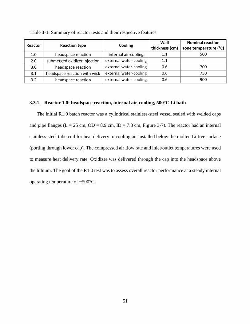
51
Table 3-1: Summary of reactor tests and their respective features
Reactor Reaction type Cooling Wall
thickness (cm) Nominal reaction
zone temperature (°C)
1.0 headspace reaction internal air-cooling 1.1 500
2.0 submerged oxidizer injection external water-cooling 1.1 -
3.0 headspace reaction external water-cooling 0.6 700
3.1 headspace reaction with wick external water-cooling 0.6 750
3.2 headspace reaction external water-cooling 0.6 900
3.3.1. Reactor 1.0: headspace reaction, internal air-cooling, 500°C Li bath
The initial R1.0 batch reactor was a cylindrical stainless-steel vessel sealed with welded caps
and pipe flanges (L = 25 cm, OD = 8.9 cm, ID = 7.8 cm, Figure 3-7). The reactor had an internal
stainless-steel tube coil for heat delivery to cooling air installed below the molten Li free surface
(porting through lower cap). The compressed air flow rate and inlet/outlet temperatures were used
to measure heat delivery rate. Oxidizer was delivered through the cap into the headspace above
the lithium. The goal of the R1.0 test was to assess overall reactor performance at a steady internal
operating temperature of ~500°C.
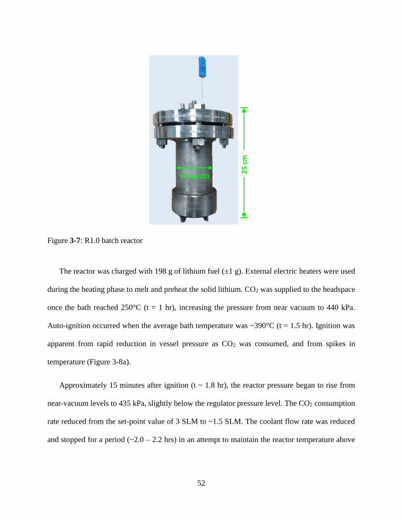
52
Figure 3-7: R1.0 batch reactor
The reactor was charged with 198 g of lithium fuel (±1 g). External electric heaters were used
during the heating phase to melt and preheat the solid lithium. CO2 was supplied to the headspace
once the bath reached 250°C (t = 1 hr), increasing the pressure from near vacuum to 440 kPa.
Auto-ignition occurred when the average bath temperature was ~390°C (t = 1.5 hr). Ignition was
apparent from rapid reduction in vessel pressure as CO2 was consumed, and from spikes in
temperature (Figure 3-8a).
Approximately 15 minutes after ignition (t ~ 1.8 hr), the reactor pressure began to rise from
near-vacuum levels to 435 kPa, slightly below the regulator pressure level. The CO2 consumption
rate reduced from the set-point value of 3 SLM to ~1.5 SLM. The coolant flow rate was reduced
and stopped for a period (~2.0 – 2.2 hrs) in an attempt to maintain the reactor temperature above
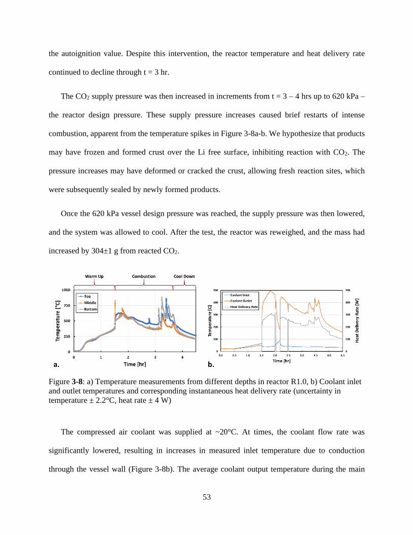
53
the autoignition value. Despite this intervention, the reactor temperature and heat delivery rate
continued to decline through t = 3 hr.
The CO2 supply pressure was then increased in increments from t = 3 – 4 hrs up to 620 kPa –
the reactor design pressure. These supply pressure increases caused brief restarts of intense
combustion, apparent from the temperature spikes in Figure 3-8a-b. We hypothesize that products
may have frozen and formed crust over the Li free surface, inhibiting reaction with CO2. The
pressure increases may have deformed or cracked the crust, allowing fresh reaction sites, which
were subsequently sealed by newly formed products.
Once the 620 kPa vessel design pressure was reached, the supply pressure was then lowered,
and the system was allowed to cool. After the test, the reactor was reweighed, and the mass had
increased by 304±1 g from reacted CO2.
Figure 3-8: a) Temperature measurements from different depths in reactor R1.0, b) Coolant inlet
and outlet temperatures and corresponding instantaneous heat delivery rate (uncertainty in
temperature ± 2.2°C, heat rate ± 4 W)
The compressed air coolant was supplied at ~20°C. At times, the coolant flow rate was
significantly lowered, resulting in increases in measured inlet temperature due to conduction
through the vessel wall (Figure 3-8b). The average coolant output temperature during the main
54
period of combustion (t = 1.5 – 3.8 hr) was 370°C. Measurements indicate an average heat delivery
rate to the cooling system of ~231 ± 4 W.
To analyze the distribution of products in the reactor and quantify unreacted lithium volume,
X-ray CT imaging was performed of the reactor vessel (using General Electric v|tome|x L300
nano/microC). Figure 3-9 presents a cross-section from the R1.0 scan.
Figure 3-9: Reactor 1.0 CT scan cross-section
In this CT scan cross-section, darker zones toward the bottom can be inferred to be patches of
unreacted elemental lithium, which is relatively transparent to X-rays. The lighter section toward
the top of the reactor is inferred to be mostly filled with reaction products containing carbon and
oxygen. This supports the hypothesis that combustion products formed a crust over the lithium
free surface. The circular marks are cross-sections of the embedded stainless-steel cooling coil
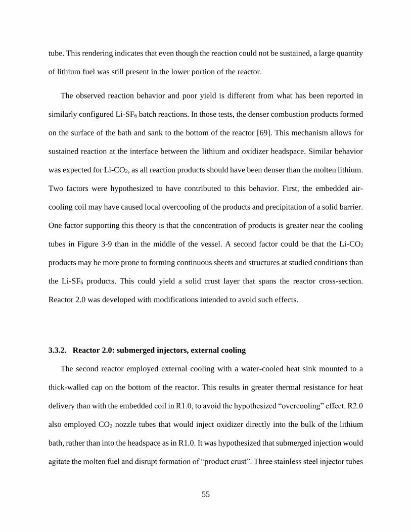
55
tube. This rendering indicates that even though the reaction could not be sustained, a large quantity
of lithium fuel was still present in the lower portion of the reactor.
The observed reaction behavior and poor yield is different from what has been reported in
similarly configured Li-SF6 batch reactions. In those tests, the denser combustion products formed
on the surface of the bath and sank to the bottom of the reactor [69]. This mechanism allows for
sustained reaction at the interface between the lithium and oxidizer headspace. Similar behavior
was expected for Li-CO2, as all reaction products should have been denser than the molten lithium.
Two factors were hypothesized to have contributed to this behavior. First, the embedded air-
cooling coil may have caused local overcooling of the products and precipitation of a solid barrier.
One factor supporting this theory is that the concentration of products is greater near the cooling
tubes in Figure 3-9 than in the middle of the vessel. A second factor could be that the Li-CO2
products may be more prone to forming continuous sheets and structures at studied conditions than
the Li-SF6 products. This could yield a solid crust layer that spans the reactor cross-section.
Reactor 2.0 was developed with modifications intended to avoid such effects.
3.3.2. Reactor 2.0: submerged injectors, external cooling
The second reactor employed external cooling with a water-cooled heat sink mounted to a
thick-walled cap on the bottom of the reactor. This results in greater thermal resistance for heat
delivery than with the embedded coil in R1.0, to avoid the hypothesized “overcooling” effect. R2.0
also employed CO2 nozzle tubes that would inject oxidizer directly into the bulk of the lithium
bath, rather than into the headspace as in R1.0. It was hypothesized that submerged injection would
agitate the molten fuel and disrupt formation of “product crust”. Three stainless steel injector tubes
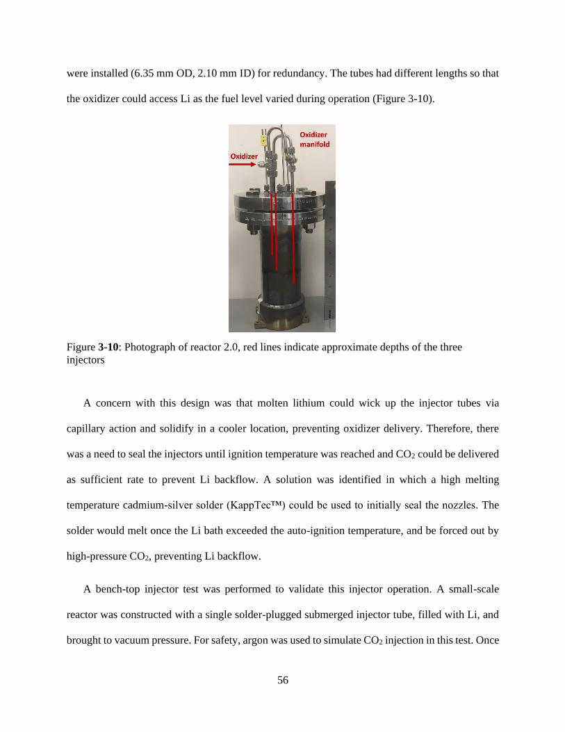
56
were installed (6.35 mm OD, 2.10 mm ID) for redundancy. The tubes had different lengths so that
the oxidizer could access Li as the fuel level varied during operation (Figure 3-10).
Figure 3-10: Photograph of reactor 2.0, red lines indicate approximate depths of the three
injectors
A concern with this design was that molten lithium could wick up the injector tubes via
capillary action and solidify in a cooler location, preventing oxidizer delivery. Therefore, there
was a need to seal the injectors until ignition temperature was reached and CO2 could be delivered
as sufficient rate to prevent Li backflow. A solution was identified in which a high melting
temperature cadmium-silver solder (KappTec™) could be used to initially seal the nozzles. The
solder would melt once the Li bath exceeded the auto-ignition temperature, and be forced out by
high-pressure CO2, preventing Li backflow.
A bench-top injector test was performed to validate this injector operation. A small-scale
reactor was constructed with a single solder-plugged submerged injector tube, filled with Li, and
brought to vacuum pressure. For safety, argon was used to simulate CO2 injection in this test. Once
57
the reactor reached 410°C, the internal pressure quickly rose to that of the argon supply. This
indicated that the solder plug would melt and allow flow only once sufficient temperatures were
reached.
Based on this proof-of-concept finding, the R2.0 injectors were sealed with the solder. The
reactor was prepared and preheated, following a similar procedure to that for R1.0. Once ignition
temperatures were reached, the reaction started, but then ended quickly. For a short time (~15
minutes) oxidizer flow was measured and the bath temperature increased. However, the pressure
equalized between the oxidizer supply and the reactor headspace, and the bath temperature
decreased below the ignition temperature. This indicated that oxidizer could no longer reach the
lithium. Attempts to restart the reaction by increasing CO2 supply pressure and heating using the
electric heater were unsuccessful.
Figure 3-11 shows post-test CT scan cross-sections of the reactor (color map applied).
Blockages are visible near the ends of all three injectors (appear red-to-white with color map).
These are hypothesized to be combustion products that filled the injectors and impeded flow of
oxidizer into the reactor.
58
Figure 3-11: Post-test CT-scan cross-sections of Reactor 2.0, indicating blockages in the injector
tubes
Due to the challenges encountered with the submerged injectors (R2.0), later tests (R3.0-3.2)
employed headspace injection, and other approaches were explored to improve yield.
3.3.3. Reactor 3.0: headspace reaction, external cooling, 700°C Li bath
As in R2.0, external cooling was employed for R3.0-3.2 to avoid local overcooling in the Li
bath. For these tests, reaction heat was delivered with an external copper collar heat sink clamped
around the reactor at the anticipated height of the free surface – the main reaction front (rendering
in Figure 3-12). A compressible graphite sheet was installed between the vessel and collar to act
as a thermal interface material. A copper bar extended from the collar and was cooled at the end
with a water-cooled heat sink. Three thermocouples were installed along the length of the bar to
act as a 1-D conduction heat flow sensor. The whole assembly was insulated during operation to
limit heat loss.
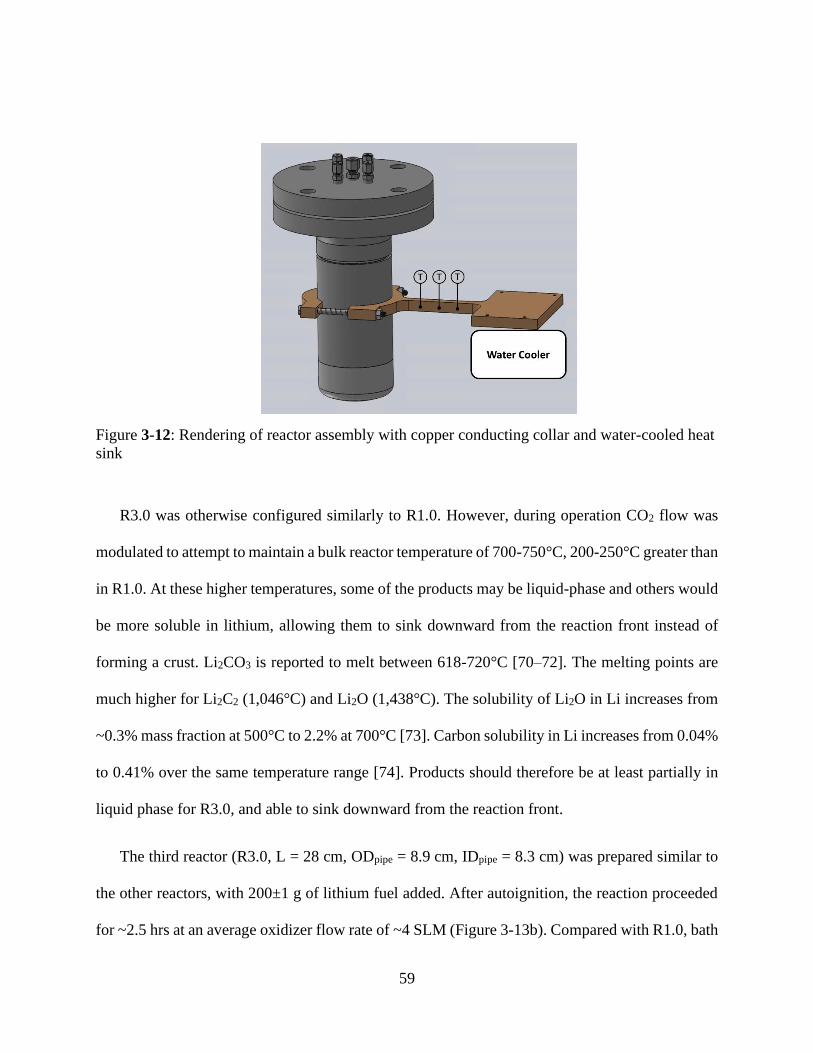
59
Figure 3-12: Rendering of reactor assembly with copper conducting collar and water-cooled heat
sink
R3.0 was otherwise configured similarly to R1.0. However, during operation CO2 flow was
modulated to attempt to maintain a bulk reactor temperature of 700-750°C, 200-250°C greater than
in R1.0. At these higher temperatures, some of the products may be liquid-phase and others would
be more soluble in lithium, allowing them to sink downward from the reaction front instead of
forming a crust. Li2CO3 is reported to melt between 618-720°C [70–72]. The melting points are
much higher for Li2C2 (1,046°C) and Li2O (1,438°C). The solubility of Li2O in Li increases from
~0.3% mass fraction at 500°C to 2.2% at 700°C [73]. Carbon solubility in Li increases from 0.04%
to 0.41% over the same temperature range [74]. Products should therefore be at least partially in
liquid phase for R3.0, and able to sink downward from the reaction front.
The third reactor (R3.0, L = 28 cm, ODpipe = 8.9 cm, IDpipe = 8.3 cm) was prepared similar to
the other reactors, with 200±1 g of lithium fuel added. After autoignition, the reaction proceeded
for ~2.5 hrs at an average oxidizer flow rate of ~4 SLM (Figure 3-13b). Compared with R1.0, bath
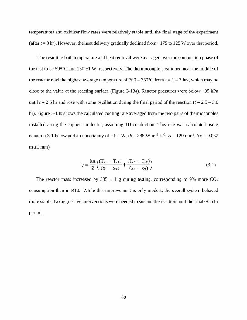
60
temperatures and oxidizer flow rates were relatively stable until the final stage of the experiment
(after t = 3 hr). However, the heat delivery gradually declined from ~175 to 125 W over that period.
The resulting bath temperature and heat removal were averaged over the combustion phase of
the test to be 598°C and 150 ±1 W, respectively. The thermocouple positioned near the middle of
the reactor read the highest average temperature of 700 – 750°C from t = 1 – 3 hrs, which may be
close to the value at the reacting surface (Figure 3-13a). Reactor pressures were below ~35 kPa
until t = 2.5 hr and rose with some oscillation during the final period of the reaction (t = 2.5 – 3.0
hr). Figure 3-13b shows the calculated cooling rate averaged from the two pairs of thermocouples
installed along the copper conductor, assuming 1D conduction. This rate was calculated using
equation 3-1 below and an uncertainty of ±1-2 W, (k = 388 W m-1 K-1, A = 129 mm2, ∆𝑥 = 0.032
m ±1 mm).
Q =kA
2(
(Tx1 − Tx2)
(x1 − x2)+
(Tx2 − Tx3)
(x2 − x3)) (3-1)
The reactor mass increased by 335 ± 1 g during testing, corresponding to 9% more CO2
consumption than in R1.0. While this improvement is only modest, the overall system behaved
more stable. No aggressive interventions were needed to sustain the reaction until the final ~0.5 hr
period.
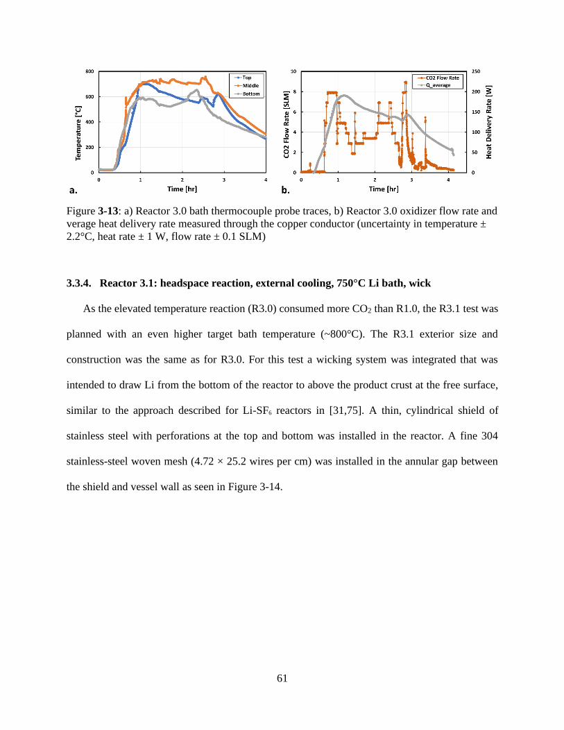
61
Figure 3-13: a) Reactor 3.0 bath thermocouple probe traces, b) Reactor 3.0 oxidizer flow rate and
verage heat delivery rate measured through the copper conductor (uncertainty in temperature ±
2.2°C, heat rate ± 1 W, flow rate ± 0.1 SLM)
3.3.4. Reactor 3.1: headspace reaction, external cooling, 750°C Li bath, wick
As the elevated temperature reaction (R3.0) consumed more CO2 than R1.0, the R3.1 test was
planned with an even higher target bath temperature (~800°C). The R3.1 exterior size and
construction was the same as for R3.0. For this test a wicking system was integrated that was
intended to draw Li from the bottom of the reactor to above the product crust at the free surface,
similar to the approach described for Li-SF6 reactors in [31,75]. A thin, cylindrical shield of
stainless steel with perforations at the top and bottom was installed in the reactor. A fine 304
stainless-steel woven mesh (4.72 × 25.2 wires per cm) was installed in the annular gap between
the shield and vessel wall as seen in Figure 3-14.
62
Figure 3-14: a) R3.1 with stainless steel shield and wire mesh installed, b) drawing of the shield
before it was rolled and welded (right)
It was hypothesized that any molten, unreacted lithium at the bottom of the reactor would wet
this mesh and rise by capillary action between the shield and reactor wall to the top of the reactor,
where it would evaporate into the headspace and react. Li is reported to be non-wetting on 316-SS
at its melting temperature (180.5°C), but its wettability increases in temperature with a contact
angle of 25° at 450°C [76,77]. This suggests that the Li should be nearly fully wetting on the mesh,
and could achieve a capillary rise of ~1.4 m.
R3.1 was prepared and preheated similarly to R3.0, with 200 ± 1 g of Li fuel. During
combustion, the oxidizer flow rate was modulated to maintain a bulk reactor temperature of
~800°C. The reaction proceeded consistently, as in R3.0, with no aggressive interventions to
oxidizer supply pressure or cooling system needed before the final phase of reaction. Combustion
proceeded for ~2.3 hr with an average oxidizer flow rate of ~4.6 SLM (Figure 3-15b). Peak bath
temperatures were 740 – 770°C for most of the combustion period (Figure 3-15a). The average
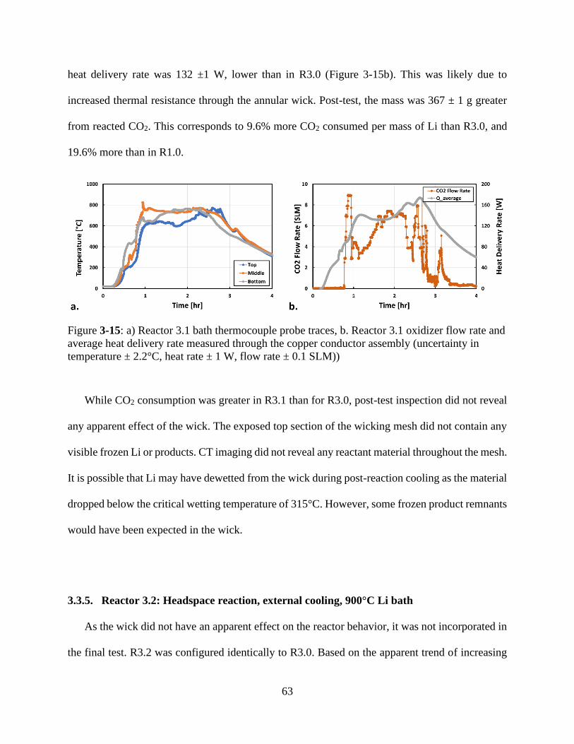
63
heat delivery rate was 132 ±1 W, lower than in R3.0 (Figure 3-15b). This was likely due to
increased thermal resistance through the annular wick. Post-test, the mass was 367 ± 1 g greater
from reacted CO2. This corresponds to 9.6% more CO2 consumed per mass of Li than R3.0, and
19.6% more than in R1.0.
Figure 3-15: a) Reactor 3.1 bath thermocouple probe traces, b. Reactor 3.1 oxidizer flow rate and
average heat delivery rate measured through the copper conductor assembly (uncertainty in
temperature ± 2.2°C, heat rate ± 1 W, flow rate ± 0.1 SLM))
While CO2 consumption was greater in R3.1 than for R3.0, post-test inspection did not reveal
any apparent effect of the wick. The exposed top section of the wicking mesh did not contain any
visible frozen Li or products. CT imaging did not reveal any reactant material throughout the mesh.
It is possible that Li may have dewetted from the wick during post-reaction cooling as the material
dropped below the critical wetting temperature of 315°C. However, some frozen product remnants
would have been expected in the wick.
3.3.5. Reactor 3.2: Headspace reaction, external cooling, 900°C Li bath
As the wick did not have an apparent effect on the reactor behavior, it was not incorporated in
the final test. R3.2 was configured identically to R3.0. Based on the apparent trend of increasing
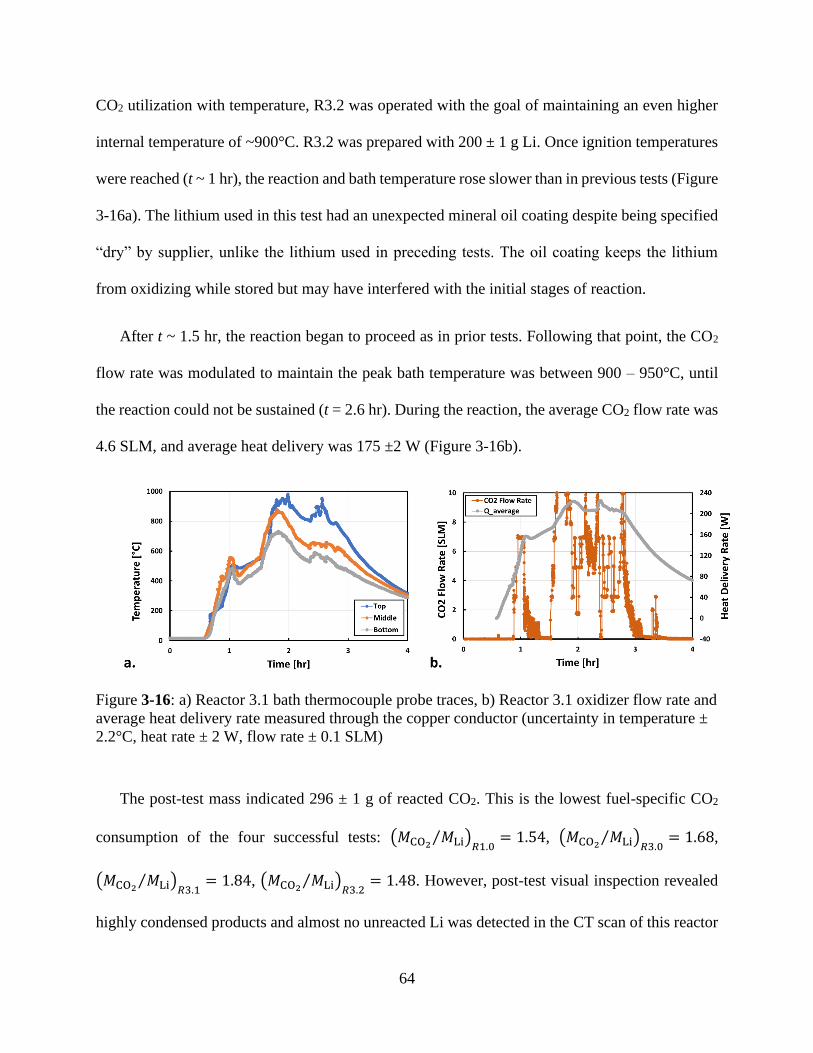
64
CO2 utilization with temperature, R3.2 was operated with the goal of maintaining an even higher
internal temperature of ~900°C. R3.2 was prepared with 200 ± 1 g Li. Once ignition temperatures
were reached (t ~ 1 hr), the reaction and bath temperature rose slower than in previous tests (Figure
3-16a). The lithium used in this test had an unexpected mineral oil coating despite being specified
“dry” by supplier, unlike the lithium used in preceding tests. The oil coating keeps the lithium
from oxidizing while stored but may have interfered with the initial stages of reaction.
After t ~ 1.5 hr, the reaction began to proceed as in prior tests. Following that point, the CO2
flow rate was modulated to maintain the peak bath temperature was between 900 – 950°C, until
the reaction could not be sustained (t = 2.6 hr). During the reaction, the average CO2 flow rate was
4.6 SLM, and average heat delivery was 175 ±2 W (Figure 3-16b).
Figure 3-16: a) Reactor 3.1 bath thermocouple probe traces, b) Reactor 3.1 oxidizer flow rate and
average heat delivery rate measured through the copper conductor (uncertainty in temperature ±
2.2°C, heat rate ± 2 W, flow rate ± 0.1 SLM)
The post-test mass indicated 296 ± 1 g of reacted CO2. This is the lowest fuel-specific CO2
consumption of the four successful tests: (𝑀CO2𝑀Li⁄ )
𝑅1.0= 1.54, (𝑀CO2
𝑀Li⁄ )𝑅3.0
= 1.68,
(𝑀CO2𝑀Li⁄ )
𝑅3.1= 1.84, (𝑀CO2
𝑀Li⁄ )𝑅3.2
= 1.48. However, post-test visual inspection revealed
highly condensed products and almost no unreacted Li was detected in the CT scan of this reactor
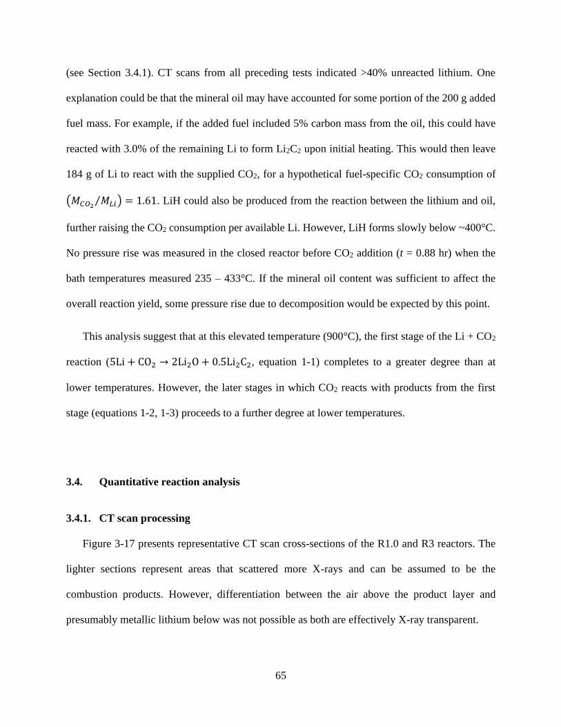
65
(see Section 3.4.1). CT scans from all preceding tests indicated >40% unreacted lithium. One
explanation could be that the mineral oil may have accounted for some portion of the 200 g added
fuel mass. For example, if the added fuel included 5% carbon mass from the oil, this could have
reacted with 3.0% of the remaining Li to form Li2C2 upon initial heating. This would then leave
184 g of Li to react with the supplied CO2, for a hypothetical fuel-specific CO2 consumption of
(𝑀𝐶𝑂2𝑀𝐿𝑖⁄ ) = 1.61. LiH could also be produced from the reaction between the lithium and oil,
further raising the CO2 consumption per available Li. However, LiH forms slowly below ~400°C.
No pressure rise was measured in the closed reactor before CO2 addition (t = 0.88 hr) when the
bath temperatures measured 235 – 433°C. If the mineral oil content was sufficient to affect the
overall reaction yield, some pressure rise due to decomposition would be expected by this point.
This analysis suggest that at this elevated temperature (900°C), the first stage of the Li + CO2
reaction (5Li + CO2 → 2Li2O + 0.5Li2C2, equation 1-1) completes to a greater degree than at
lower temperatures. However, the later stages in which CO2 reacts with products from the first
stage (equations 1-2, 1-3) proceeds to a further degree at lower temperatures.
3.4. Quantitative reaction analysis
3.4.1. CT scan processing
Figure 3-17 presents representative CT scan cross-sections of the R1.0 and R3 reactors. The
lighter sections represent areas that scattered more X-rays and can be assumed to be the
combustion products. However, differentiation between the air above the product layer and
presumably metallic lithium below was not possible as both are effectively X-ray transparent.
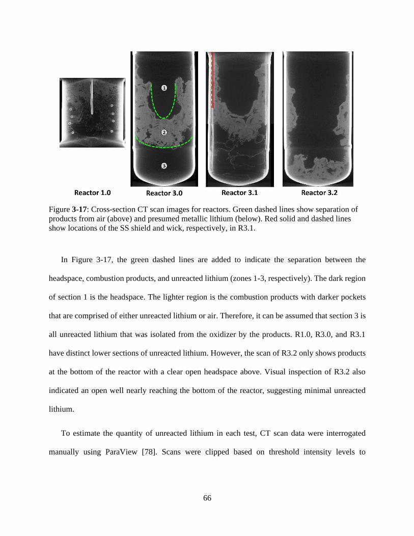
66
Figure 3-17: Cross-section CT scan images for reactors. Green dashed lines show separation of
products from air (above) and presumed metallic lithium (below). Red solid and dashed lines
show locations of the SS shield and wick, respectively, in R3.1.
In Figure 3-17, the green dashed lines are added to indicate the separation between the
headspace, combustion products, and unreacted lithium (zones 1-3, respectively). The dark region
of section 1 is the headspace. The lighter region is the combustion products with darker pockets
that are comprised of either unreacted lithium or air. Therefore, it can be assumed that section 3 is
all unreacted lithium that was isolated from the oxidizer by the products. R1.0, R3.0, and R3.1
have distinct lower sections of unreacted lithium. However, the scan of R3.2 only shows products
at the bottom of the reactor with a clear open headspace above. Visual inspection of R3.2 also
indicated an open well nearly reaching the bottom of the reactor, suggesting minimal unreacted
lithium.
To estimate the quantity of unreacted lithium in each test, CT scan data were interrogated
manually using ParaView [78]. Scans were clipped based on threshold intensity levels to
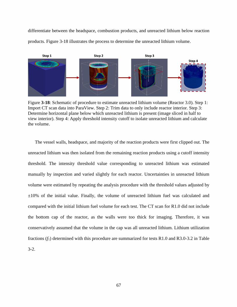
67
differentiate between the headspace, combustion products, and unreacted lithium below reaction
products. Figure 3-18 illustrates the process to determine the unreacted lithium volume.
Figure 3-18: Schematic of procedure to estimate unreacted lithium volume (Reactor 3.0). Step 1:
Import CT scan data into ParaView. Step 2: Trim data to only include reactor interior. Step 3:
Determine horizontal plane below which unreacted lithium is present (image sliced in half to
view interior). Step 4: Apply threshold intensity cutoff to isolate unreacted lithium and calculate
the volume.
The vessel walls, headspace, and majority of the reaction products were first clipped out. The
unreacted lithium was then isolated from the remaining reaction products using a cutoff intensity
threshold. The intensity threshold value corresponding to unreacted lithium was estimated
manually by inspection and varied slightly for each reactor. Uncertainties in unreacted lithium
volume were estimated by repeating the analysis procedure with the threshold values adjusted by
±10% of the initial value. Finally, the volume of unreacted lithium fuel was calculated and
compared with the initial lithium fuel volume for each test. The CT scan for R1.0 did not include
the bottom cap of the reactor, as the walls were too thick for imaging. Therefore, it was
conservatively assumed that the volume in the cap was all unreacted lithium. Lithium utilization
fractions (f1) determined with this procedure are summarized for tests R1.0 and R3.0-3.2 in Table
3-2.
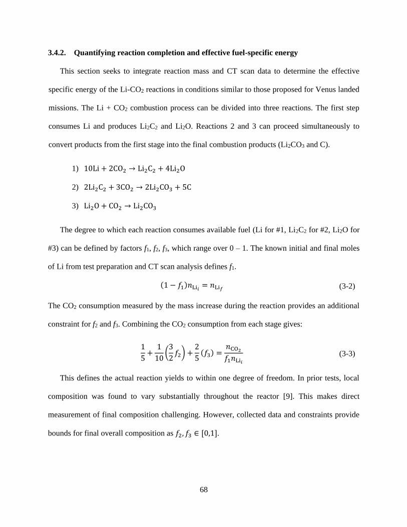
68
3.4.2. Quantifying reaction completion and effective fuel-specific energy
This section seeks to integrate reaction mass and CT scan data to determine the effective
specific energy of the Li-CO2 reactions in conditions similar to those proposed for Venus landed
missions. The Li + CO2 combustion process can be divided into three reactions. The first step
consumes Li and produces Li2C2 and Li2O. Reactions 2 and 3 can proceed simultaneously to
convert products from the first stage into the final combustion products (Li2CO3 and C).
1) 10Li + 2CO2 → Li2C2 + 4Li2O
2) 2Li2C2 + 3CO2 → 2Li2CO3 + 5C
3) Li2O + CO2 → Li2CO3
The degree to which each reaction consumes available fuel (Li for #1, Li2C2 for #2, Li2O for
#3) can be defined by factors f1, f2, f3, which range over 0 – 1. The known initial and final moles
of Li from test preparation and CT scan analysis defines f1.
(1 − 𝑓1)𝑛Li𝑖= 𝑛Li𝑓
(3-2)
The CO2 consumption measured by the mass increase during the reaction provides an additional
constraint for f2 and f3. Combining the CO2 consumption from each stage gives:
1
5+
1
10(
3
2𝑓2) +
2
5(𝑓3) =
𝑛CO2
𝑓1𝑛Li𝑖
(3-3)
This defines the actual reaction yields to within one degree of freedom. In prior tests, local
composition was found to vary substantially throughout the reactor [9]. This makes direct
measurement of final composition challenging. However, collected data and constraints provide
bounds for final overall composition as 𝑓2, 𝑓3 ∈ [0,1].
69
Temperature, mass, and Li consumption (from CT scans) are summarized for each test in Table
3-2. Based on these values, realizable ranges of yields for reactions 1-2 and 1-3 (f2, f3) and final
compositions are determined. These ranges are reported in corresponding orders (i.e., as f2
increases, f3 decreases). Reaction energy is determined from an energy balance with fuel and
product enthalpies evaluated at experimental temperatures and inlet CO2 at 470°C (Venus
ambient). The effective fuel-specific energy can be defined as the total reaction heat per mass of
Li fuel added to the reactor (𝑞Li = 𝑄 𝑚Li,i⁄ ). Because of the wide range of possible values of f2 and
f3, simple analytic uncertainty propagation was not appropriate for this quantity. Instead, a Monte-
Carlo procedure was used. The greatest effective fuel-specific energy was found at the R3.2
conditions: 25.6 ± 0.7 MJ kgLi−1.
For R1.0, R3.0, and R3.1, performed at increasing Li bath temperatures, specific CO2
consumption increased (𝑚CO2/𝑚Li = 1.52, 1.68, 1.84). However, in the highest temperature test
(R3.2), 𝑚CO2/𝑚Li is only 1.49. This may be due to endothermic decomposition of lithium
carbonate (Li2CO3 → Li2O + CO2). Ktalkherman et al. (2009) report that this reaction occurs
above ~800°C, which was only reached in R3.2 [79]. Li2CO3 produced from reaction #2 may be
converted to Li2O, releasing CO2, and reaction #3 may proceed minimally. This is supported by
the high Li2O content (62 – 68%) and low Li2C2 (16 – 22%) and Li2CO3 (10 – 16%) contents
inferred for R3.2 in Table 3-2. As the lower temperature reactor tests can form more Li2CO3, they
produce more heat per unit of Li that is actually utilized (𝑞Li,reacted = 𝑄 (𝑓1 𝑚Li,i)⁄ ). For tests
R1.0 and R3.1, 𝑞Li,reacted values are close to the theoretical limit of 45.1 MJ kg-1. If methods can
be found to improve lithium utilization at such temperatures, such as agitation of the Li bath as
attempted in R2.0, system performance may be greatly improved.
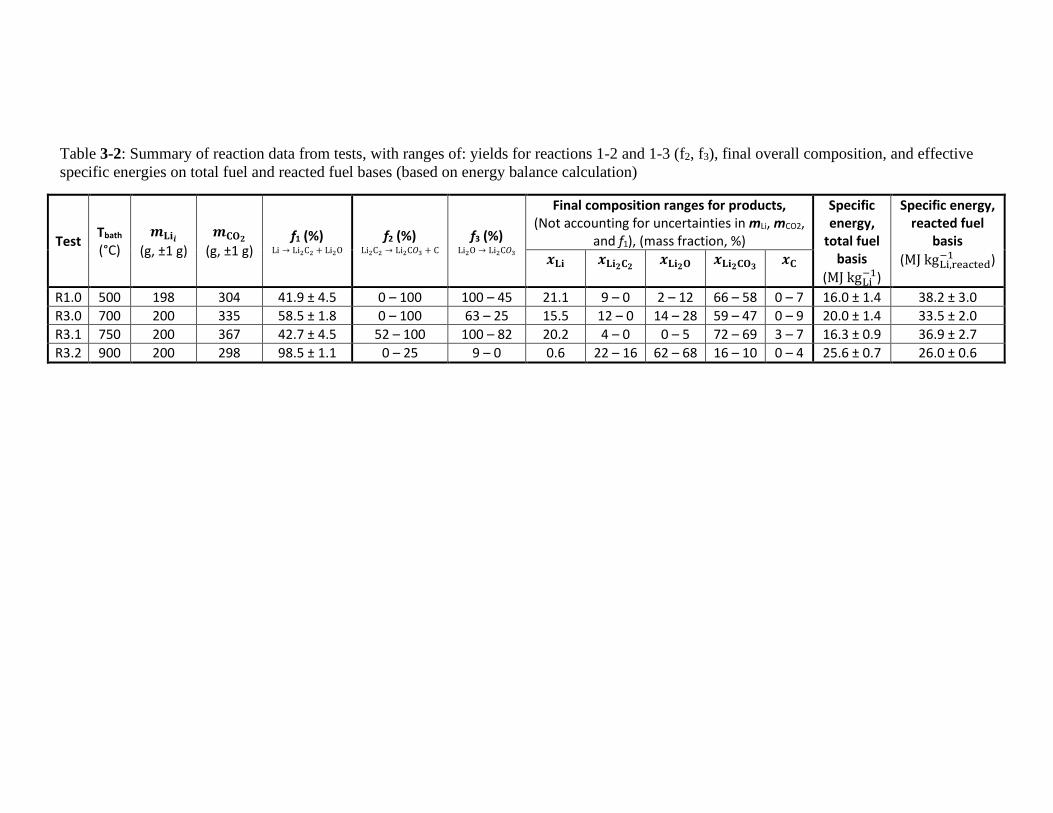
Table 3-2: Summary of reaction data from tests, with ranges of: yields for reactions 1-2 and 1-3 (f2, f3), final overall composition, and effective
specific energies on total fuel and reacted fuel bases (based on energy balance calculation)
Test Tbath (°C)
𝒎𝐋𝐢𝒊
(g, ±1 g)
𝒎𝐂𝐎𝟐
(g, ±1 g) f1 (%)
Li → Li2C2 + Li2O f2 (%)
Li2C2 → Li2C𝑂3 + C f3 (%)
Li2O → Li2C𝑂3
Final composition ranges for products, (Not accounting for uncertainties in mLi, mCO2,
and f1), (mass fraction, %)
Specific energy,
total fuel basis
(MJ kgLi−1)
Specific energy, reacted fuel
basis
(MJ kgLi,reacted−1 ) 𝒙𝐋𝐢 𝒙𝐋𝐢𝟐𝐂𝟐
𝒙𝐋𝐢𝟐𝐎 𝒙𝐋𝐢𝟐𝐂𝐎𝟑 𝒙𝐂
R1.0 500 198 304 41.9 ± 4.5 0 – 100 100 – 45 21.1 9 – 0 2 – 12 66 – 58 0 – 7 16.0 ± 1.4 38.2 ± 3.0
R3.0 700 200 335 58.5 ± 1.8 0 – 100 63 – 25 15.5 12 – 0 14 – 28 59 – 47 0 – 9 20.0 ± 1.4 33.5 ± 2.0
R3.1 750 200 367 42.7 ± 4.5 52 – 100 100 – 82 20.2 4 – 0 0 – 5 72 – 69 3 – 7 16.3 ± 0.9 36.9 ± 2.7
R3.2 900 200 298 98.5 ± 1.1 0 – 25 9 – 0 0.6 22 – 16 62 – 68 16 – 10 0 – 4 25.6 ± 0.7 26.0 ± 0.6
71
3.5. Conclusion
The goal of this chapter was to perform an experimental evaluation and validation of a lithium
and carbon-dioxide batch reactor. In this investigation, a series of Li-CO2 batch reactors were
constructed and tested to determine the effective specific energy that can be achieved in chemical
fueled ISRU power systems proposed for Venus surface missions. Five reactors were evaluated
over a range of operating temperatures (500 – 900°C) and with different mechanisms for
simulating heat delivery and contacting Li fuel with CO2 oxidizer. Mass flow, pressure, and
temperature data were collected during tests to provide insights into the reaction processes. Mass
measurements and post-test CT scans were employed to determine overall reactant utilization and
empirical fuel-specific energies.
At lower temperatures, a thick product crust formed over the molten Li, limiting fuel
utilization. At ~900°C, nearly all Li fuel was reacted (>98%), yielding a fuel-specific energy of
25.6 ± 0.7 MJ kgLi−1. This is close to the specific energy assumed (27.5 MJ kgLi
−1) in prior conceptual
and modeling studies of chemical-fuel powered Venus landers [15,80]. At lower temperatures (500
– 750°C), specific energy per reacted Li mass is greater (32 – 41 MJ kg-1). However, only 40 –
60% Li utilization was achieved in those tests. Attempts to increase yield by agitating the fuel bath
with submerged injectors and bypass product crust with wicks were unsuccessful here. These
results highlight the potential chemical combustion power systems have to enable Venus surface
missions. To fully realize this potential and continue to mature this technology for future lander
missions, additional research and development is required. Future work will include additional
batch reactor experiments to optimize the lithium utilization with the specific energy, insulation,
and reaction rate control to regulate the heat delivery/cooling rate. Additionally, to take advantage
of this high specific energy, a heat engine that can survive and operate efficiently at Venus

72
conditions will be required. Chapter 4 will select a heat engine for Venus surface operations and
outline a laboratory scale system for cycle characterization and development.

73
Chapter 4
Thermodynamic Analysis of a Mercury Vapor
Rankine Cycle for a Venus Lander
74
Conditions on Venus render traditional space power systems ineffective. Chemical combustion
and RTG powered systems have been proposed to increase mission duration beyond what is viable
with battery power [13,15,81,82]. To achieve this longer duration a heat engine concept must be
identified that can operate effectively in the Venus surface environment. The goal of this chapter
is to perform an analysis and design of a viable Venus surface heat engine. A thermodynamic cycle
will be down selected, a working fluid identified, and a scaled-down configuration defined that
can be assessed at laboratory scale. Lastly, a list of engineering requirements will be provided for
a future mission enabled by this technology.
4.1. Heat engine selection for Venus application
A future heat engine for a Venus lander needs to be able to survive and operate efficiently in
the 460°C, 93 bar environment, while providing 100’s of Watts of electrical power and 1000’s of
Watts of cooling. No heat engine technology has been demonstrated that can deliver necessary
reliability, power output levels, or efficiency for a long-lived Venus in-situ explorer mission. Any
heat engine whether solid state or thermo-mechanical will have the challenge of either material or
working fluid selection for operations at the extreme temperatures found at the Venusian surface.
Thermoelectric generators (TEGs) are used in current radioisotope power systems (RPS), but
have poor efficiencies, especially at high heat sink temperatures. No TEG materials have yet been
proven for Venus conditions, additionally the highest temperature option only has a projected
energy density of 35 Whe kg-1 (CMO-32-62S: TH = 900°C, TC = 470°C [83]). Thermophotovoltaic
(TPV) systems couple IR photovoltaics with spectrally tuned radiators, theoretically enabling high
75
efficiencies. However, current TPV cell materials (GaSb [84]), must be cooled below 200°C to
prevent junction diffusion and failure [85,86].
Long-lived Venus surface mission concepts allot the majority of system power to mechanically
refrigerate sensitive instruments [6,13,81,87]. Due to extreme temperature effects, the only electric
motor developed for such conditions, from Honeybee Robotics, has a peak efficiency of 43% [88].
Solid-state power conversion systems therefore may require more than two times the capacity of
equivalent thermo-mechanical cycles that can deliver shaft work to directly drive refrigeration
compressors. This challenge to efficiently provide refrigeration and current lack of high
temperature materials make solid-state power systems less promising. Therefore, thermo-
mechanical cycles are the focus of this analysis.
Reciprocating gas cycles (e.g., Stirling, thermo-acoustic) deliver high efficiencies at low sink
temperatures, and represent three of the four technologies down-selected by NASA for the
dynamic RPS program [89,90]. However, based on conversations with leading technology
developers the critical translational mechanisms and flexure materials would fail on Venus.
Turbine-based cycles are mechanically simpler than reciprocating machinery, reducing such
challenges.
Gas turbine cycles (Brayton/recuperated Brayton) can deliver high efficiencies (>45%) at
earth-like conditions (temperature ratio TR = TH / TC ~ 1525°C / 27°C = 6). Such performance
levels stem from the much greater work available in expanding hot gas than required for
compressing cool gas. For Venus surface conditions, the turbine inlet temperature is above
maximum material working temperatures and requires active blade cooling. On Venus, where
turbine cooling may be infeasible or limited, maximum viable temperature ratios may be TH / TC
~ 927°C / 467°C ~ 1.6, due to the high surface temperature. An Engineering Equation Solver (EES)
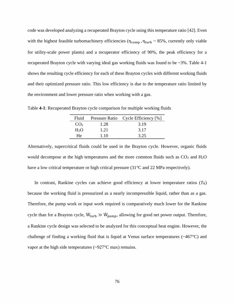
76
code was developed analyzing a recuperated Brayton cycle using this temperature ratio [42]. Even
with the highest feasible turbomachinery efficiencies (ηcomp , ηturb ~ 85%, currently only viable
for utility-scale power plants) and a recuperator efficiency of 90%, the peak efficiency for a
recuperated Brayton cycle with varying ideal gas working fluids was found to be ~3%. Table 4-1
shows the resulting cycle efficiency for each of these Brayton cycles with different working fluids
and their optimized pressure ratio. This low efficiency is due to the temperature ratio limited by
the environment and lower pressure ratio when working with a gas.
Table 4-1: Recuperated Brayton cycle comparison for multiple working fluids
Fluid Pressure Ratio Cycle Efficiency [%]
CO2 1.28 3.19
H2O 1.21 3.17
He 1.10 3.25
Alternatively, supercritical fluids could be used in the Brayton cycle. However, organic fluids
would decompose at the high temperatures and the more common fluids such as CO2 and H2O
have a low critical temperature or high critical pressure (31°C and 22 MPa respectively).
In contrast, Rankine cycles can achieve good efficiency at lower temperature ratios (TR)
because the working fluid is pressurized as a nearly incompressible liquid, rather than as a gas.
Therefore, the pump work or input work required is comparatively much lower for the Rankine
cycle than for a Brayton cycle, Wturb ≫ Wpump, allowing for good net power output. Therefore,
a Rankine cycle design was selected to be analyzed for this conceptual heat engine. However, the
challenge of finding a working fluid that is liquid at Venus surface temperatures (~467°C) and
vapor at the high side temperatures (~927°C max) remains.
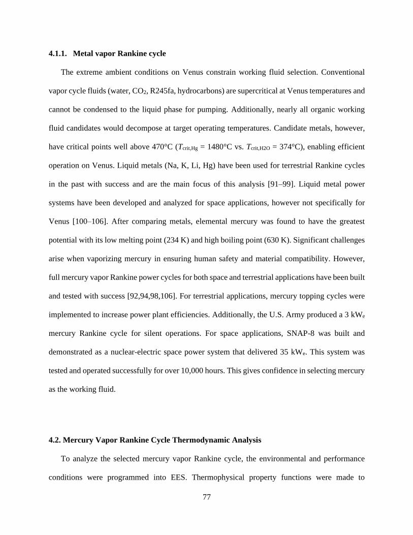
77
4.1.1. Metal vapor Rankine cycle
The extreme ambient conditions on Venus constrain working fluid selection. Conventional
vapor cycle fluids (water, CO2, R245fa, hydrocarbons) are supercritical at Venus temperatures and
cannot be condensed to the liquid phase for pumping. Additionally, nearly all organic working
fluid candidates would decompose at target operating temperatures. Candidate metals, however,
have critical points well above 470°C (Tcrit,Hg = 1480°C vs. Tcrit,H2O = 374°C), enabling efficient
operation on Venus. Liquid metals (Na, K, Li, Hg) have been used for terrestrial Rankine cycles
in the past with success and are the main focus of this analysis [91–99]. Liquid metal power
systems have been developed and analyzed for space applications, however not specifically for
Venus [100–106]. After comparing metals, elemental mercury was found to have the greatest
potential with its low melting point (234 K) and high boiling point (630 K). Significant challenges
arise when vaporizing mercury in ensuring human safety and material compatibility. However,
full mercury vapor Rankine power cycles for both space and terrestrial applications have been built
and tested with success [92,94,98,106]. For terrestrial applications, mercury topping cycles were
implemented to increase power plant efficiencies. Additionally, the U.S. Army produced a 3 kWe
mercury Rankine cycle for silent operations. For space applications, SNAP-8 was built and
demonstrated as a nuclear-electric space power system that delivered 35 kWe. This system was
tested and operated successfully for over 10,000 hours. This gives confidence in selecting mercury
as the working fluid.
4.2. Mercury Vapor Rankine Cycle Thermodynamic Analysis
To analyze the selected mercury vapor Rankine cycle, the environmental and performance
conditions were programmed into EES. Thermophysical property functions were made to
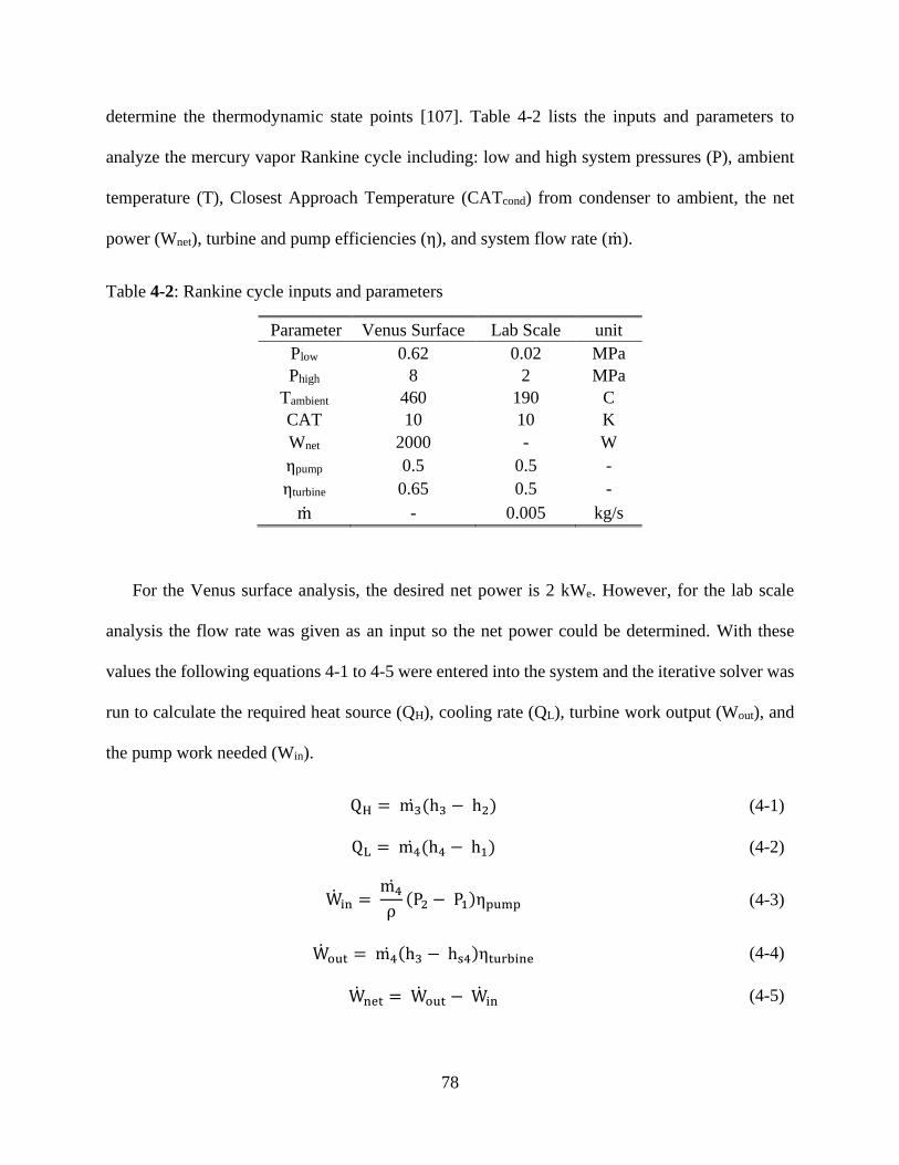
78
determine the thermodynamic state points [107]. Table 4-2 lists the inputs and parameters to
analyze the mercury vapor Rankine cycle including: low and high system pressures (P), ambient
temperature (T), Closest Approach Temperature (CATcond) from condenser to ambient, the net
power (Wnet), turbine and pump efficiencies (η), and system flow rate (m).
Table 4-2: Rankine cycle inputs and parameters
Parameter Venus Surface Lab Scale unit
Plow 0.62 0.02 MPa
Phigh 8 2 MPa
Tambient 460 190 C
CAT 10 10 K
Wnet 2000 - W
ηpump 0.5 0.5 -
ηturbine 0.65 0.5 -
m - 0.005 kg/s
For the Venus surface analysis, the desired net power is 2 kWe. However, for the lab scale
analysis the flow rate was given as an input so the net power could be determined. With these
values the following equations 4-1 to 4-5 were entered into the system and the iterative solver was
run to calculate the required heat source (QH), cooling rate (QL), turbine work output (Wout), and
the pump work needed (Win).
QH = m3 (h3 − h2) (4-1)
QL = m4 (h4 − h1) (4-2)
Win = m4
ρ
(P2 − P1)ηpump (4-3)
Wout = m4 (h3 − hs4)ηturbine (4-4)
Wnet = Wout − Win (4-5)
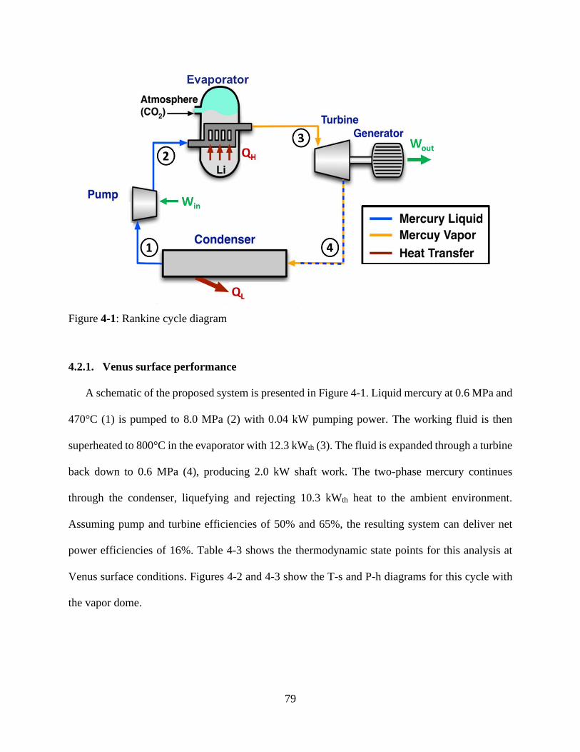
79
Figure 4-1: Rankine cycle diagram
4.2.1. Venus surface performance
A schematic of the proposed system is presented in Figure 4-1. Liquid mercury at 0.6 MPa and
470°C (1) is pumped to 8.0 MPa (2) with 0.04 kW pumping power. The working fluid is then
superheated to 800°C in the evaporator with 12.3 kWth (3). The fluid is expanded through a turbine
back down to 0.6 MPa (4), producing 2.0 kW shaft work. The two-phase mercury continues
through the condenser, liquefying and rejecting 10.3 kWth heat to the ambient environment.
Assuming pump and turbine efficiencies of 50% and 65%, the resulting system can deliver net
power efficiencies of 16%. Table 4-3 shows the thermodynamic state points for this analysis at
Venus surface conditions. Figures 4-2 and 4-3 show the T-s and P-h diagrams for this cycle with
the vapor dome.
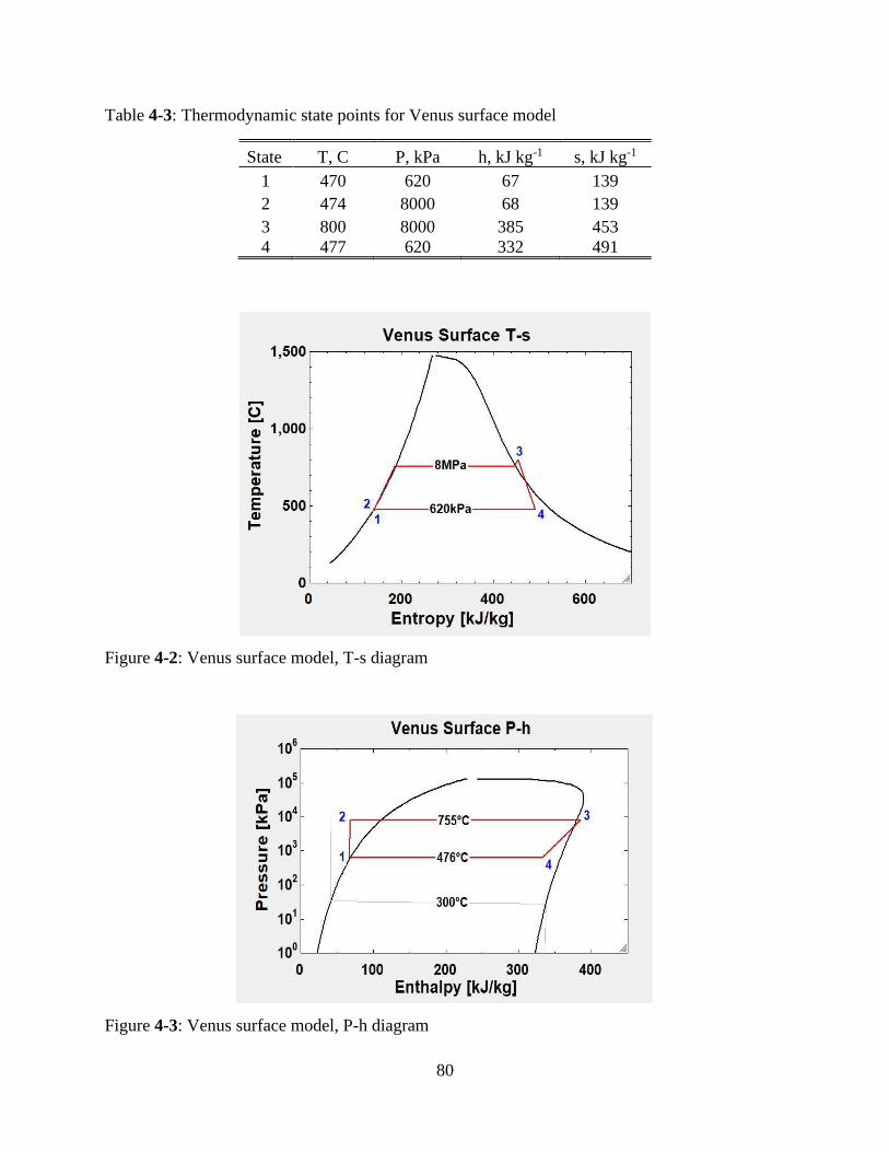
80
Table 4-3: Thermodynamic state points for Venus surface model
State T, C P, kPa h, kJ kg-1 s, kJ kg-1
1 470 620 67 139
2 474 8000 68 139
3 800 8000 385 453
4 477 620 332 491
Figure 4-2: Venus surface model, T-s diagram
Figure 4-3: Venus surface model, P-h diagram
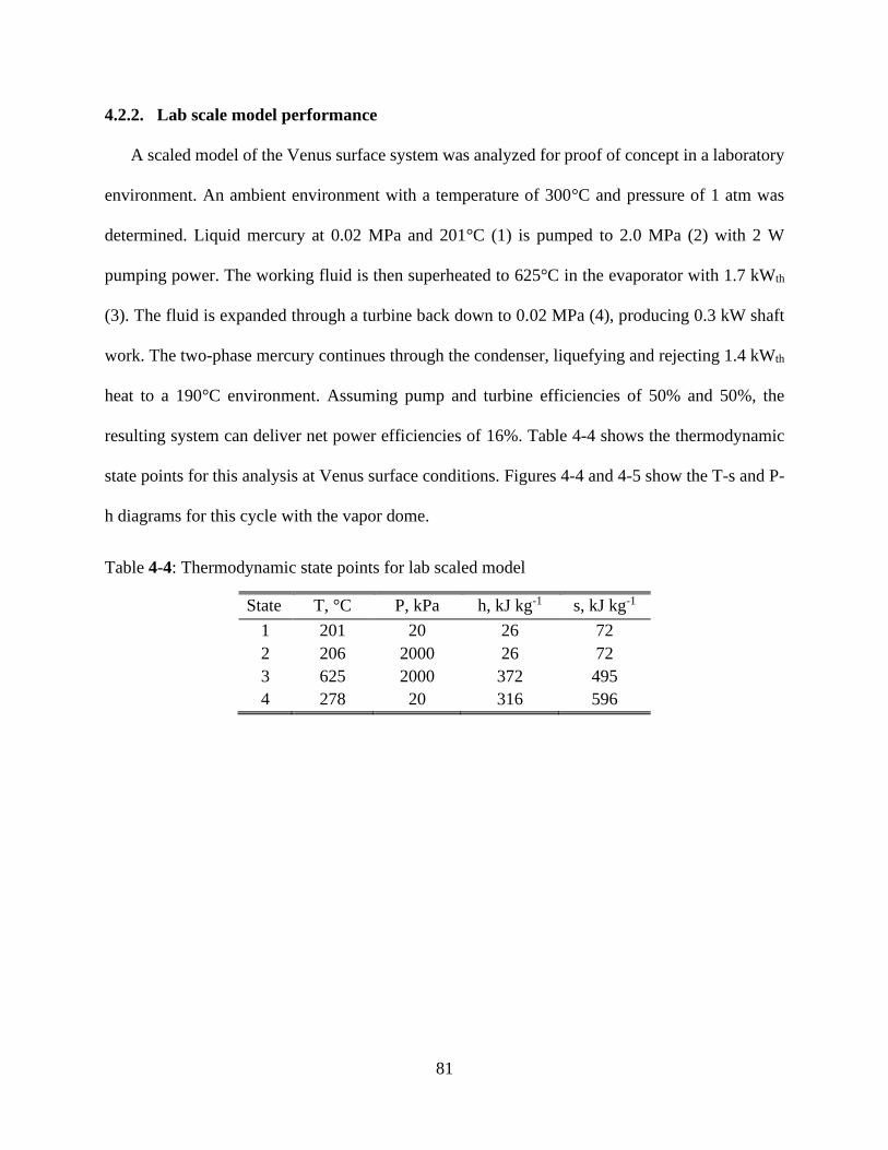
81
4.2.2. Lab scale model performance
A scaled model of the Venus surface system was analyzed for proof of concept in a laboratory
environment. An ambient environment with a temperature of 300°C and pressure of 1 atm was
determined. Liquid mercury at 0.02 MPa and 201°C (1) is pumped to 2.0 MPa (2) with 2 W
pumping power. The working fluid is then superheated to 625°C in the evaporator with 1.7 kWth
(3). The fluid is expanded through a turbine back down to 0.02 MPa (4), producing 0.3 kW shaft
work. The two-phase mercury continues through the condenser, liquefying and rejecting 1.4 kWth
heat to a 190°C environment. Assuming pump and turbine efficiencies of 50% and 50%, the
resulting system can deliver net power efficiencies of 16%. Table 4-4 shows the thermodynamic
state points for this analysis at Venus surface conditions. Figures 4-4 and 4-5 show the T-s and P-
h diagrams for this cycle with the vapor dome.
Table 4-4: Thermodynamic state points for lab scaled model
State T, °C P, kPa h, kJ kg-1 s, kJ kg-1
1 201 20 26 72
2 206 2000 26 72
3 625 2000 372 495
4 278 20 316 596
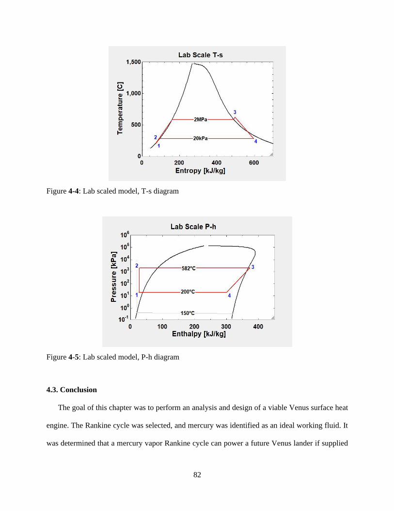
82
Figure 4-4: Lab scaled model, T-s diagram
Figure 4-5: Lab scaled model, P-h diagram
4.3. Conclusion
The goal of this chapter was to perform an analysis and design of a viable Venus surface heat
engine. The Rankine cycle was selected, and mercury was identified as an ideal working fluid. It
was determined that a mercury vapor Rankine cycle can power a future Venus lander if supplied
83
12.3 kW of thermal heat. This system will provide 2.0 kW of shaft power to the spacecraft. This
cycle performed with a power efficiency of 16%. This matches the desired Stirling engine
efficiency in the Section 2.2.1 analysis and shows the Rankine cycle meets the performance
requirements to supply enough power for a Venus lander when coupled with a chemical
combustion power system. A scaled-down configuration was defined that can be assessed at
laboratory scale. Chapter 5 presents the current progress on an experimental test stand based on
this configuration.
The current analysis did not include the design of the heat-rejection system from the condenser
to the Venus environment. Analysis have been performed for heat rejection on the surface of Venus
and can be used as a baseline for future designs [19]. Future analysis and experimentation will be
required to design and test this system in actual Venus conditions. Additionally, future work will
be required to evaluate potential spacecraft cooling when coupled with a refrigeration cycle.
4.3.1. Engineering Requirements
• A turbine will be required to supply 2 kW of shaft power by expanding 800°C vapor mercury
with a pressure ratio of 12.9
• With 42 W of power a pump will be required to increase the pressure of 470°C liquid mercury
by a pressure ratio of 12.9, at a flow rate of 0.04 kg s-1
• A liquid mercury condenser will be required to reject 10.3 kW of heat to the 460°C Venus
environment. The CAT and UA determined for this heat exchanger are 10 K and 620 W K-1
respectively

84
• A heat source will be required to provide at least 12.3 kWth to superheat the mercury working
fluid with a heat exchanger UA of 411 W K-1
85
Chapter 5
Experimental Mercury Vapor Rankine Cycle Testing
for a Venus Lander
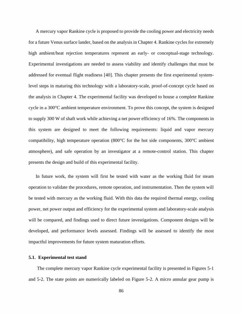
86
A mercury vapor Rankine cycle is proposed to provide the cooling power and electricity needs
for a future Venus surface lander, based on the analysis in Chapter 4. Rankine cycles for extremely
high ambient/heat rejection temperatures represent an early- or conceptual-stage technology.
Experimental investigations are needed to assess viability and identify challenges that must be
addressed for eventual flight readiness [40]. This chapter presents the first experimental system-
level steps in maturing this technology with a laboratory-scale, proof-of-concept cycle based on
the analysis in Chapter 4. The experimental facility was developed to house a complete Rankine
cycle in a 300°C ambient temperature environment. To prove this concept, the system is designed
to supply 300 W of shaft work while achieving a net power efficiency of 16%. The components in
this system are designed to meet the following requirements: liquid and vapor mercury
compatibility, high temperature operation (800°C for the hot side components, 300°C ambient
atmosphere), and safe operation by an investigator at a remote-control station. This chapter
presents the design and build of this experimental facility.
In future work, the system will first be tested with water as the working fluid for steam
operation to validate the procedures, remote operation, and instrumentation. Then the system will
be tested with mercury as the working fluid. With this data the required thermal energy, cooling
power, net power output and efficiency for the experimental system and laboratory-scale analysis
will be compared, and findings used to direct future investigations. Component designs will be
developed, and performance levels assessed. Findings will be assessed to identify the most
impactful improvements for future system maturation efforts.
5.1. Experimental test stand
The complete mercury vapor Rankine cycle experimental facility is presented in Figures 5-1
and 5-2. The state points are numerically labeled on Figure 5-2. A micro annular gear pump is
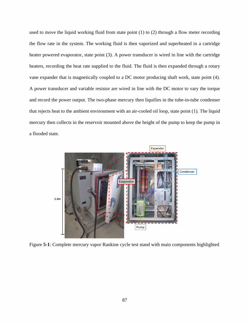
87
used to move the liquid working fluid from state point (1) to (2) through a flow meter recording
the flow rate in the system. The working fluid is then vaporized and superheated in a cartridge
heater powered evaporator, state point (3). A power transducer is wired in line with the cartridge
heaters, recording the heat rate supplied to the fluid. The fluid is then expanded through a rotary
vane expander that is magnetically coupled to a DC motor producing shaft work, state point (4).
A power transducer and variable resistor are wired in line with the DC motor to vary the torque
and record the power output. The two-phase mercury then liquifies in the tube-in-tube condenser
that rejects heat to the ambient environment with an air-cooled oil loop, state point (1). The liquid
mercury then collects in the reservoir mounted above the height of the pump to keep the pump in
a flooded state.
Figure 5-1: Complete mercury vapor Rankine cycle test stand with main components highlighted
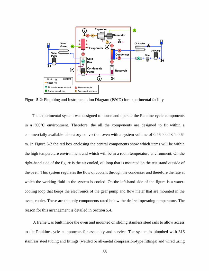
88
Figure 5-2: Plumbing and Instrumentation Diagram (P&ID) for experimental facility
The experimental system was designed to house and operate the Rankine cycle components
in a 300°C environment. Therefore, the all the components are designed to fit within a
commercially available laboratory convection oven with a system volume of 0.46 × 0.43 × 0.64
m. In Figure 5-2 the red box enclosing the central components show which items will be within
the high temperature environment and which will be in a room temperature environment. On the
right-hand side of the figure is the air cooled, oil loop that is mounted on the test stand outside of
the oven. This system regulates the flow of coolant through the condenser and therefore the rate at
which the working fluid in the system is cooled. On the left-hand side of the figure is a water-
cooling loop that keeps the electronics of the gear pump and flow meter that are mounted in the
oven, cooler. These are the only components rated below the desired operating temperature. The
reason for this arrangement is detailed in Section 5.4.
A frame was built inside the oven and mounted on sliding stainless steel rails to allow access
to the Rankine cycle components for assembly and service. The system is plumbed with 316
stainless steel tubing and fittings (welded or all-metal compression-type fittings) and wired using
89
high temperature fiberglass insulated cabling. All the electronics and instrumentation are routed to
an external room-temperature electronics enclosure on the test stand. A satellite control box allows
operator monitoring and control from up to 6-meter distance. Figure 5-3 shows the satellite control
box with the power and instrumentation switches turned on and the USB signal cable from the data
acquisition unit streaming to a computer.
Figure 5-3: Satellite control box
A National Instruments cDAQ-9174 is used to record the data from the test stand. This DAQ
was installed with a C series NI-9213 thermocouple module and a NI-9203 current input module.
The LabView user interface code is shown in Figure 5-4.
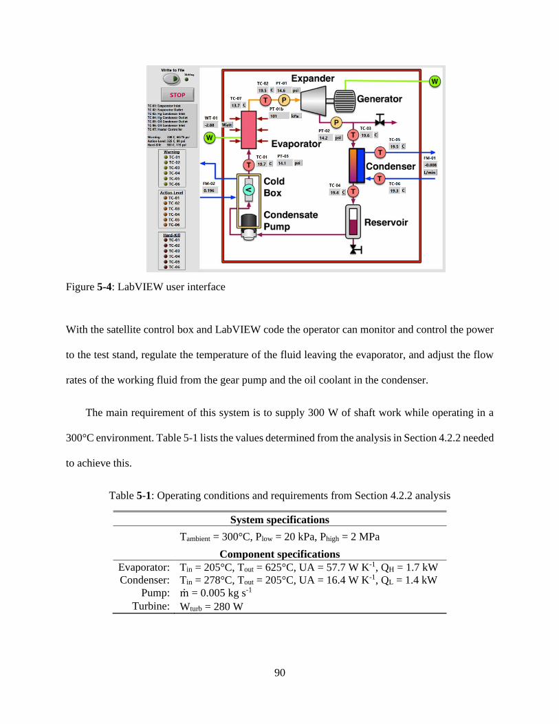
90
Figure 5-4: LabVIEW user interface
With the satellite control box and LabVIEW code the operator can monitor and control the power
to the test stand, regulate the temperature of the fluid leaving the evaporator, and adjust the flow
rates of the working fluid from the gear pump and the oil coolant in the condenser.
The main requirement of this system is to supply 300 W of shaft work while operating in a
300°C environment. Table 5-1 lists the values determined from the analysis in Section 4.2.2 needed
to achieve this.
Table 5-1: Operating conditions and requirements from Section 4.2.2 analysis
System specifications
Tambient = 300°C, Plow = 20 kPa, Phigh = 2 MPa
Component specifications
Evaporator: Tin = 205°C, Tout = 625°C, UA = 57.7 W K-1, QH = 1.7 kW
Condenser: Tin = 278°C, Tout = 205°C, UA = 16.4 W K-1, QL = 1.4 kW
Pump: m = 0.005 kg s-1
Turbine: Wturb = 280 W
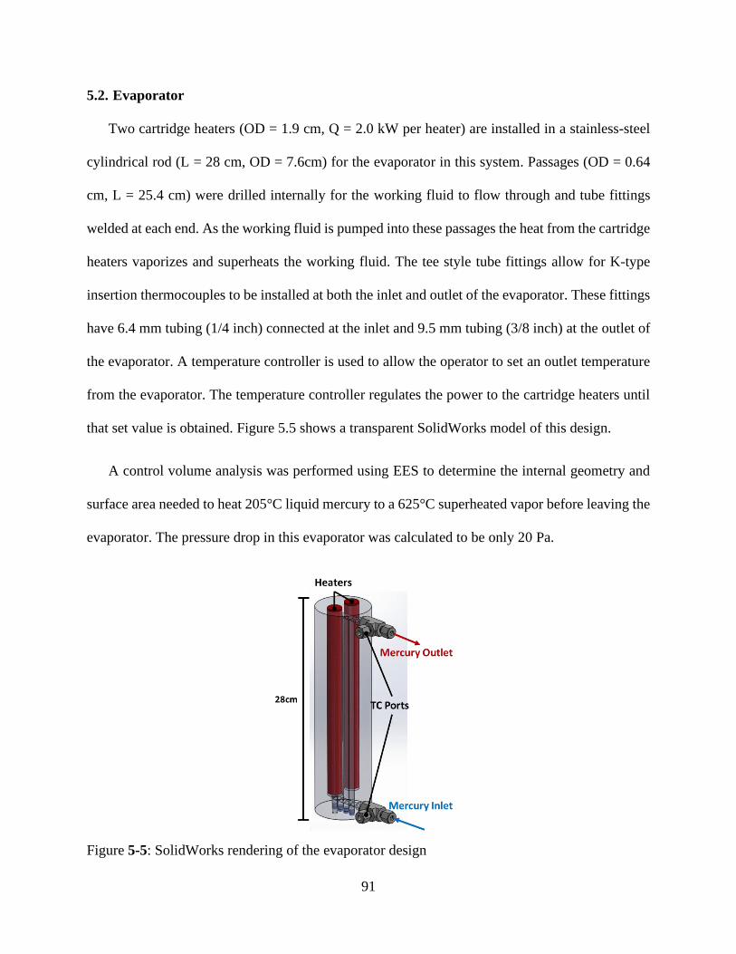
91
5.2. Evaporator
Two cartridge heaters (OD = 1.9 cm, Q = 2.0 kW per heater) are installed in a stainless-steel
cylindrical rod (L = 28 cm, OD = 7.6cm) for the evaporator in this system. Passages (OD = 0.64
cm, L = 25.4 cm) were drilled internally for the working fluid to flow through and tube fittings
welded at each end. As the working fluid is pumped into these passages the heat from the cartridge
heaters vaporizes and superheats the working fluid. The tee style tube fittings allow for K-type
insertion thermocouples to be installed at both the inlet and outlet of the evaporator. These fittings
have 6.4 mm tubing (1/4 inch) connected at the inlet and 9.5 mm tubing (3/8 inch) at the outlet of
the evaporator. A temperature controller is used to allow the operator to set an outlet temperature
from the evaporator. The temperature controller regulates the power to the cartridge heaters until
that set value is obtained. Figure 5.5 shows a transparent SolidWorks model of this design.
A control volume analysis was performed using EES to determine the internal geometry and
surface area needed to heat 205°C liquid mercury to a 625°C superheated vapor before leaving the
evaporator. The pressure drop in this evaporator was calculated to be only 20 Pa.
Figure 5-5: SolidWorks rendering of the evaporator design
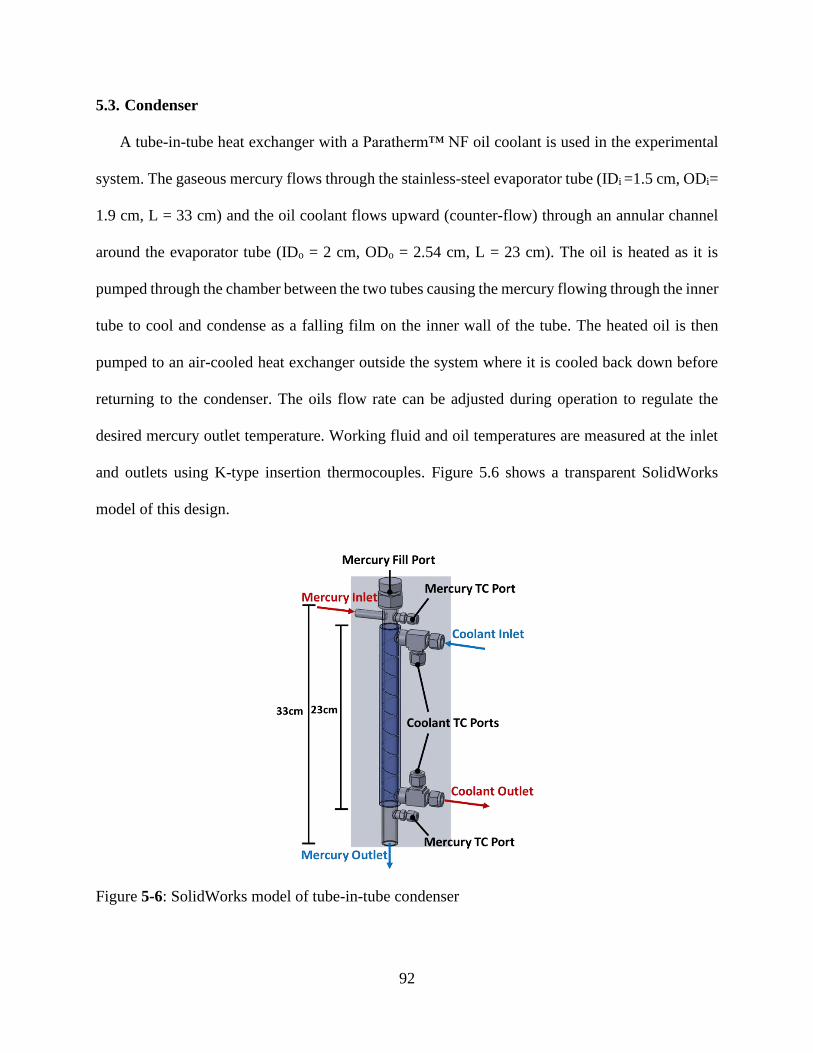
92
5.3. Condenser
A tube-in-tube heat exchanger with a Paratherm™ NF oil coolant is used in the experimental
system. The gaseous mercury flows through the stainless-steel evaporator tube (IDi =1.5 cm, ODi=
1.9 cm, L = 33 cm) and the oil coolant flows upward (counter-flow) through an annular channel
around the evaporator tube (IDo = 2 cm, ODo = 2.54 cm, L = 23 cm). The oil is heated as it is
pumped through the chamber between the two tubes causing the mercury flowing through the inner
tube to cool and condense as a falling film on the inner wall of the tube. The heated oil is then
pumped to an air-cooled heat exchanger outside the system where it is cooled back down before
returning to the condenser. The oils flow rate can be adjusted during operation to regulate the
desired mercury outlet temperature. Working fluid and oil temperatures are measured at the inlet
and outlets using K-type insertion thermocouples. Figure 5.6 shows a transparent SolidWorks
model of this design.
Figure 5-6: SolidWorks model of tube-in-tube condenser
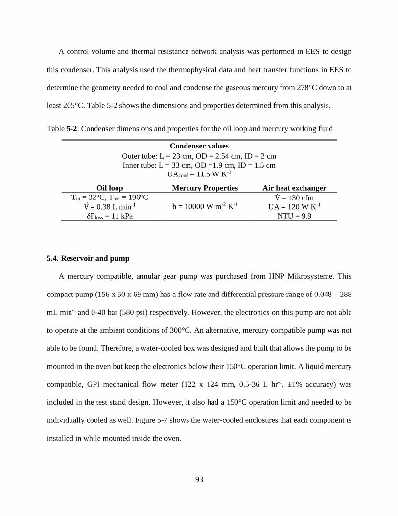
93
A control volume and thermal resistance network analysis was performed in EES to design
this condenser. This analysis used the thermophysical data and heat transfer functions in EES to
determine the geometry needed to cool and condense the gaseous mercury from 278°C down to at
least 205°C. Table 5-2 shows the dimensions and properties determined from this analysis.
Table 5-2: Condenser dimensions and properties for the oil loop and mercury working fluid
Condenser values
Outer tube: L = 23 cm, OD = 2.54 cm, ID = 2 cm
Inner tube: L = 33 cm, OD =1.9 cm, ID = 1.5 cm
UAcond = 11.5 W K-1
Oil loop Mercury Properties Air heat exchanger
Tin = 32°C, Tout = 196°C
V = 0.38 L min-1
δPloss = 11 kPa
h = 10000 W m-2 K-1 V = 130 cfm
UA = 120 W K-1
NTU = 9.9
5.4. Reservoir and pump
A mercury compatible, annular gear pump was purchased from HNP Mikrosysteme. This
compact pump (156 x 50 x 69 mm) has a flow rate and differential pressure range of 0.048 – 288
mL min-1 and 0-40 bar (580 psi) respectively. However, the electronics on this pump are not able
to operate at the ambient conditions of 300°C. An alternative, mercury compatible pump was not
able to be found. Therefore, a water-cooled box was designed and built that allows the pump to be
mounted in the oven but keep the electronics below their 150°C operation limit. A liquid mercury
compatible, GPI mechanical flow meter (122 x 124 mm, 0.5-36 L hr-1, ±1% accuracy) was
included in the test stand design. However, it also had a 150°C operation limit and needed to be
individually cooled as well. Figure 5-7 shows the water-cooled enclosures that each component is
installed in while mounted inside the oven.
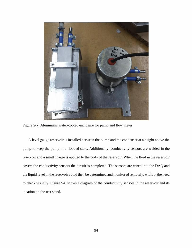
94
Figure 5-7: Aluminum, water-cooled enclosure for pump and flow meter
A level gauge reservoir is installed between the pump and the condenser at a height above the
pump to keep the pump in a flooded state. Additionally, conductivity sensors are welded in the
reservoir and a small charge is applied to the body of the reservoir. When the fluid in the reservoir
covers the conductivity sensors the circuit is completed. The sensors are wired into the DAQ and
the liquid level in the reservoir could then be determined and monitored remotely, without the need
to check visually. Figure 5-8 shows a diagram of the conductivity sensors in the reservoir and its
location on the test stand.
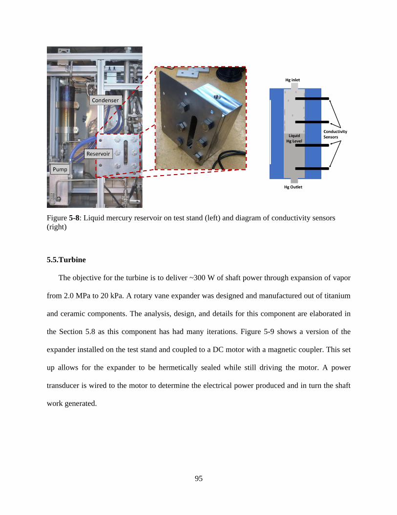
95
Figure 5-8: Liquid mercury reservoir on test stand (left) and diagram of conductivity sensors
(right)
5.5.Turbine
The objective for the turbine is to deliver ~300 W of shaft power through expansion of vapor
from 2.0 MPa to 20 kPa. A rotary vane expander was designed and manufactured out of titanium
and ceramic components. The analysis, design, and details for this component are elaborated in
the Section 5.8 as this component has had many iterations. Figure 5-9 shows a version of the
expander installed on the test stand and coupled to a DC motor with a magnetic coupler. This set
up allows for the expander to be hermetically sealed while still driving the motor. A power
transducer is wired to the motor to determine the electrical power produced and in turn the shaft
work generated.
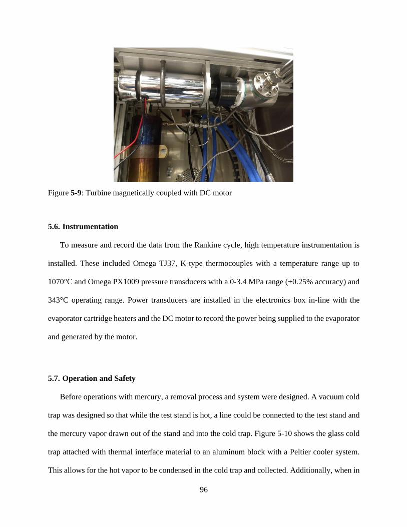
96
Figure 5-9: Turbine magnetically coupled with DC motor
5.6. Instrumentation
To measure and record the data from the Rankine cycle, high temperature instrumentation is
installed. These included Omega TJ37, K-type thermocouples with a temperature range up to
1070°C and Omega PX1009 pressure transducers with a 0-3.4 MPa range (±0.25% accuracy) and
343°C operating range. Power transducers are installed in the electronics box in-line with the
evaporator cartridge heaters and the DC motor to record the power being supplied to the evaporator
and generated by the motor.
5.7. Operation and Safety
Before operations with mercury, a removal process and system were designed. A vacuum cold
trap was designed so that while the test stand is hot, a line could be connected to the test stand and
the mercury vapor drawn out of the stand and into the cold trap. Figure 5-10 shows the glass cold
trap attached with thermal interface material to an aluminum block with a Peltier cooler system.
This allows for the hot vapor to be condensed in the cold trap and collected. Additionally, when in
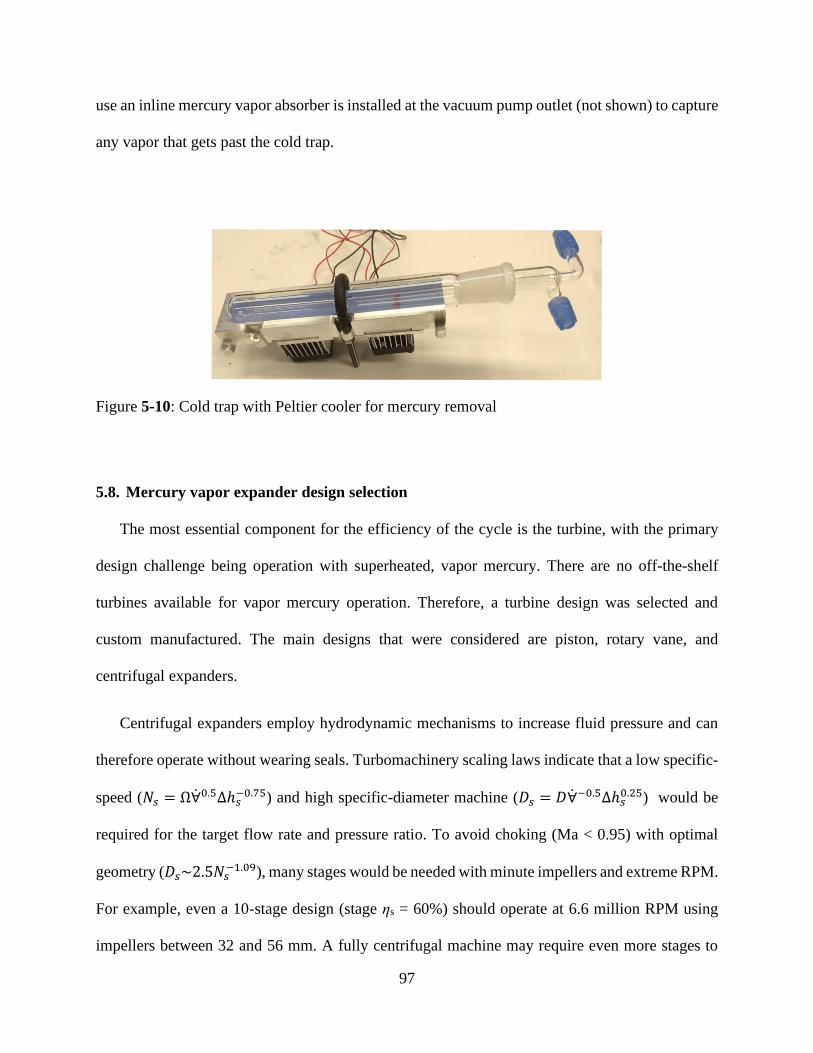
97
use an inline mercury vapor absorber is installed at the vacuum pump outlet (not shown) to capture
any vapor that gets past the cold trap.
Figure 5-10: Cold trap with Peltier cooler for mercury removal
5.8. Mercury vapor expander design selection
The most essential component for the efficiency of the cycle is the turbine, with the primary
design challenge being operation with superheated, vapor mercury. There are no off-the-shelf
turbines available for vapor mercury operation. Therefore, a turbine design was selected and
custom manufactured. The main designs that were considered are piston, rotary vane, and
centrifugal expanders.
Centrifugal expanders employ hydrodynamic mechanisms to increase fluid pressure and can
therefore operate without wearing seals. Turbomachinery scaling laws indicate that a low specific-
speed (𝑁𝑠 = Ω∀0.5Δℎ𝑠−0.75) and high specific-diameter machine (𝐷𝑠 = 𝐷∀−0.5Δℎ𝑠
0.25) would be
required for the target flow rate and pressure ratio. To avoid choking (Ma < 0.95) with optimal
geometry (𝐷𝑠~2.5𝑁𝑠−1.09), many stages would be needed with minute impellers and extreme RPM.
For example, even a 10-stage design (stage ηs = 60%) should operate at 6.6 million RPM using
impellers between 32 and 56 mm. A fully centrifugal machine may require even more stages to
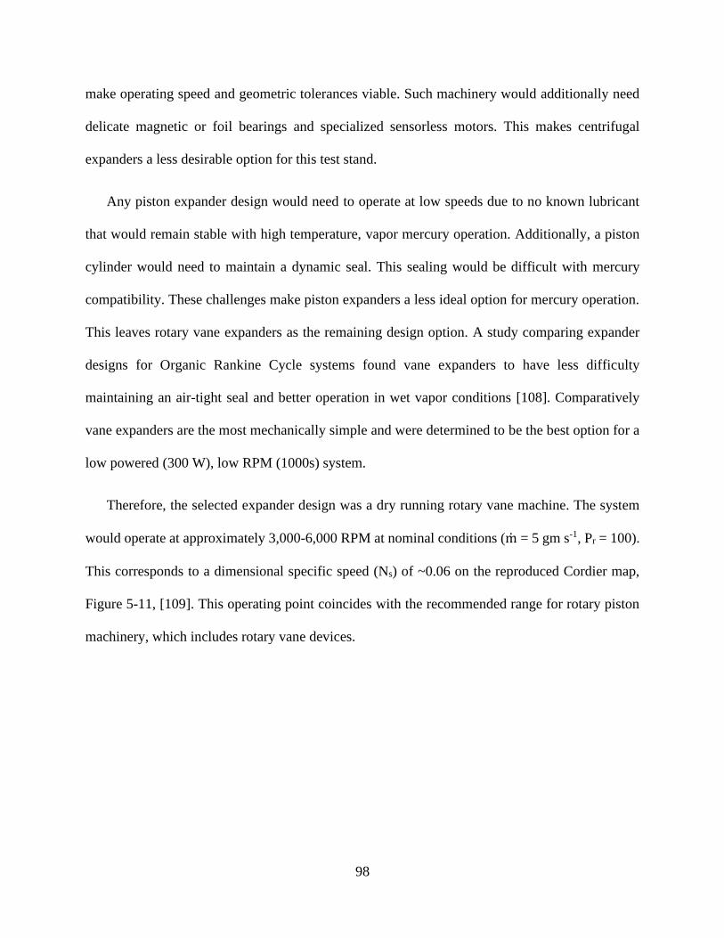
98
make operating speed and geometric tolerances viable. Such machinery would additionally need
delicate magnetic or foil bearings and specialized sensorless motors. This makes centrifugal
expanders a less desirable option for this test stand.
Any piston expander design would need to operate at low speeds due to no known lubricant
that would remain stable with high temperature, vapor mercury operation. Additionally, a piston
cylinder would need to maintain a dynamic seal. This sealing would be difficult with mercury
compatibility. These challenges make piston expanders a less ideal option for mercury operation.
This leaves rotary vane expanders as the remaining design option. A study comparing expander
designs for Organic Rankine Cycle systems found vane expanders to have less difficulty
maintaining an air-tight seal and better operation in wet vapor conditions [108]. Comparatively
vane expanders are the most mechanically simple and were determined to be the best option for a
low powered (300 W), low RPM (1000s) system.
Therefore, the selected expander design was a dry running rotary vane machine. The system
would operate at approximately 3,000-6,000 RPM at nominal conditions (m = 5 gm s-1, Pr = 100).
This corresponds to a dimensional specific speed (Ns) of ~0.06 on the reproduced Cordier map,
Figure 5-11, [109]. This operating point coincides with the recommended range for rotary piston
machinery, which includes rotary vane devices.
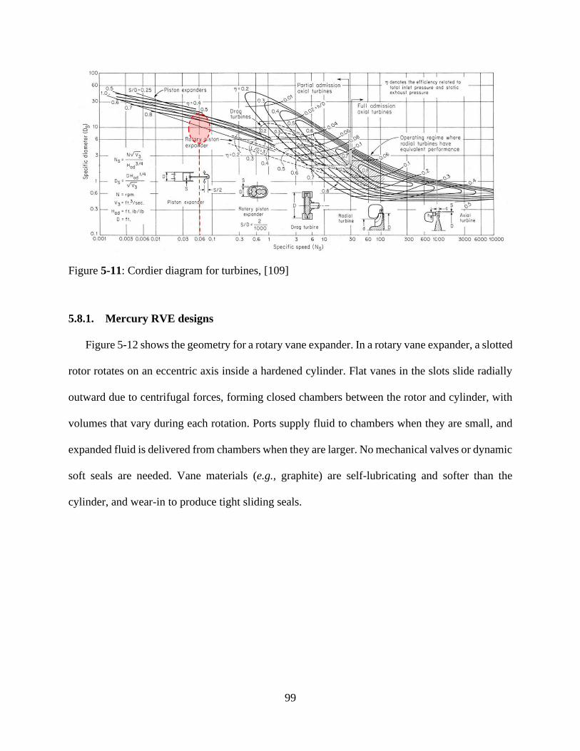
99
Figure 5-11: Cordier diagram for turbines, [109]
5.8.1. Mercury RVE designs
Figure 5-12 shows the geometry for a rotary vane expander. In a rotary vane expander, a slotted
rotor rotates on an eccentric axis inside a hardened cylinder. Flat vanes in the slots slide radially
outward due to centrifugal forces, forming closed chambers between the rotor and cylinder, with
volumes that vary during each rotation. Ports supply fluid to chambers when they are small, and
expanded fluid is delivered from chambers when they are larger. No mechanical valves or dynamic
soft seals are needed. Vane materials (e.g., graphite) are self-lubricating and softer than the
cylinder, and wear-in to produce tight sliding seals.
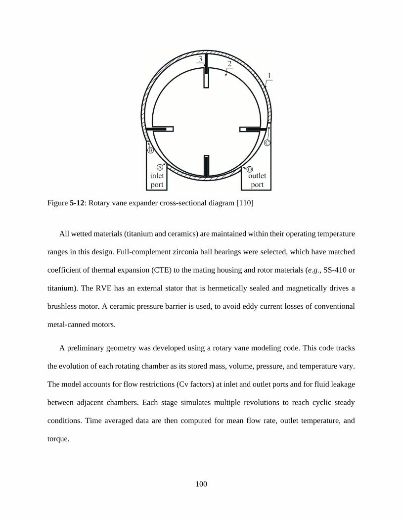
100
Figure 5-12: Rotary vane expander cross-sectional diagram [110]
All wetted materials (titanium and ceramics) are maintained within their operating temperature
ranges in this design. Full-complement zirconia ball bearings were selected, which have matched
coefficient of thermal expansion (CTE) to the mating housing and rotor materials (e.g., SS-410 or
titanium). The RVE has an external stator that is hermetically sealed and magnetically drives a
brushless motor. A ceramic pressure barrier is used, to avoid eddy current losses of conventional
metal-canned motors.
A preliminary geometry was developed using a rotary vane modeling code. This code tracks
the evolution of each rotating chamber as its stored mass, volume, pressure, and temperature vary.
The model accounts for flow restrictions (Cv factors) at inlet and outlet ports and for fluid leakage
between adjacent chambers. Each stage simulates multiple revolutions to reach cyclic steady
conditions. Time averaged data are then computed for mean flow rate, outlet temperature, and
torque.
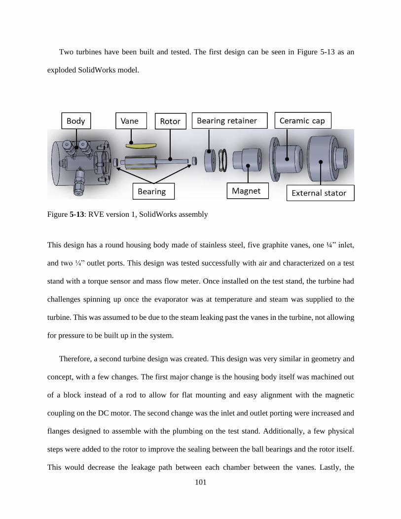
101
Two turbines have been built and tested. The first design can be seen in Figure 5-13 as an
exploded SolidWorks model.
Figure 5-13: RVE version 1, SolidWorks assembly
This design has a round housing body made of stainless steel, five graphite vanes, one ¼” inlet,
and two ¼” outlet ports. This design was tested successfully with air and characterized on a test
stand with a torque sensor and mass flow meter. Once installed on the test stand, the turbine had
challenges spinning up once the evaporator was at temperature and steam was supplied to the
turbine. This was assumed to be due to the steam leaking past the vanes in the turbine, not allowing
for pressure to be built up in the system.
Therefore, a second turbine design was created. This design was very similar in geometry and
concept, with a few changes. The first major change is the housing body itself was machined out
of a block instead of a rod to allow for flat mounting and easy alignment with the magnetic
coupling on the DC motor. The second change was the inlet and outlet porting were increased and
flanges designed to assemble with the plumbing on the test stand. Additionally, a few physical
steps were added to the rotor to improve the sealing between the ball bearings and the rotor itself.
This would decrease the leakage path between each chamber between the vanes. Lastly, the
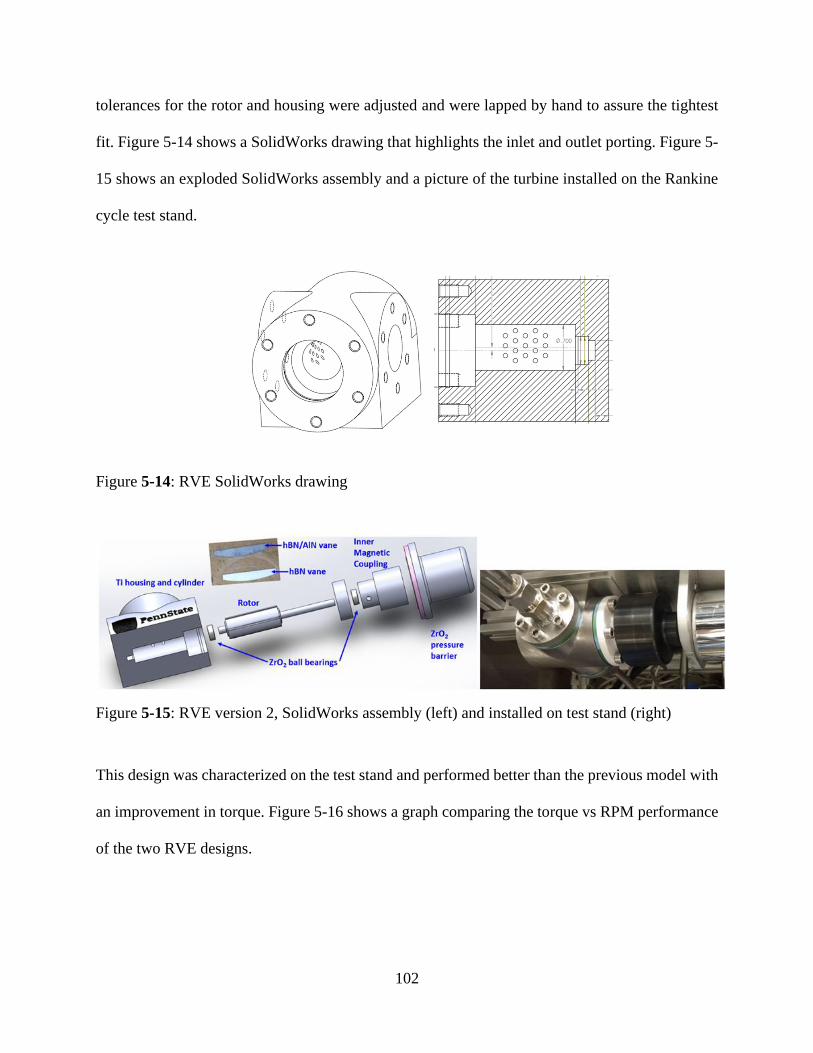
102
tolerances for the rotor and housing were adjusted and were lapped by hand to assure the tightest
fit. Figure 5-14 shows a SolidWorks drawing that highlights the inlet and outlet porting. Figure 5-
15 shows an exploded SolidWorks assembly and a picture of the turbine installed on the Rankine
cycle test stand.
Figure 5-14: RVE SolidWorks drawing
Figure 5-15: RVE version 2, SolidWorks assembly (left) and installed on test stand (right)
This design was characterized on the test stand and performed better than the previous model with
an improvement in torque. Figure 5-16 shows a graph comparing the torque vs RPM performance
of the two RVE designs.
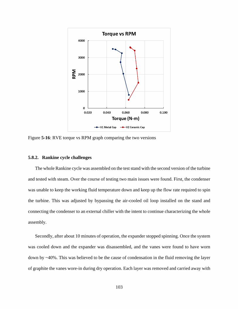
103
Figure 5-16: RVE torque vs RPM graph comparing the two versions
5.8.2. Rankine cycle challenges
The whole Rankine cycle was assembled on the test stand with the second version of the turbine
and tested with steam. Over the course of testing two main issues were found. First, the condenser
was unable to keep the working fluid temperature down and keep up the flow rate required to spin
the turbine. This was adjusted by bypassing the air-cooled oil loop installed on the stand and
connecting the condenser to an external chiller with the intent to continue characterizing the whole
assembly.
Secondly, after about 10 minutes of operation, the expander stopped spinning. Once the system
was cooled down and the expander was disassembled, and the vanes were found to have worn
down by ~40%. This was believed to be the cause of condensation in the fluid removing the layer
of graphite the vanes wore-in during dry operation. Each layer was removed and carried away with
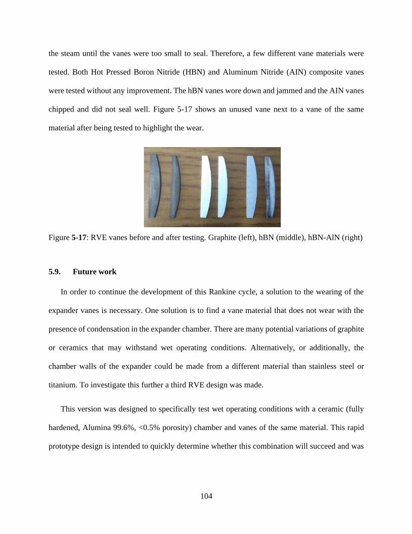
104
the steam until the vanes were too small to seal. Therefore, a few different vane materials were
tested. Both Hot Pressed Boron Nitride (HBN) and Aluminum Nitride (AIN) composite vanes
were tested without any improvement. The hBN vanes wore down and jammed and the AIN vanes
chipped and did not seal well. Figure 5-17 shows an unused vane next to a vane of the same
material after being tested to highlight the wear.
Figure 5-17: RVE vanes before and after testing. Graphite (left), hBN (middle), hBN-AlN (right)
5.9. Future work
In order to continue the development of this Rankine cycle, a solution to the wearing of the
expander vanes is necessary. One solution is to find a vane material that does not wear with the
presence of condensation in the expander chamber. There are many potential variations of graphite
or ceramics that may withstand wet operating conditions. Alternatively, or additionally, the
chamber walls of the expander could be made from a different material than stainless steel or
titanium. To investigate this further a third RVE design was made.
This version was designed to specifically test wet operating conditions with a ceramic (fully
hardened, Alumina 99.6%, <0.5% porosity) chamber and vanes of the same material. This rapid
prototype design is intended to quickly determine whether this combination will succeed and was
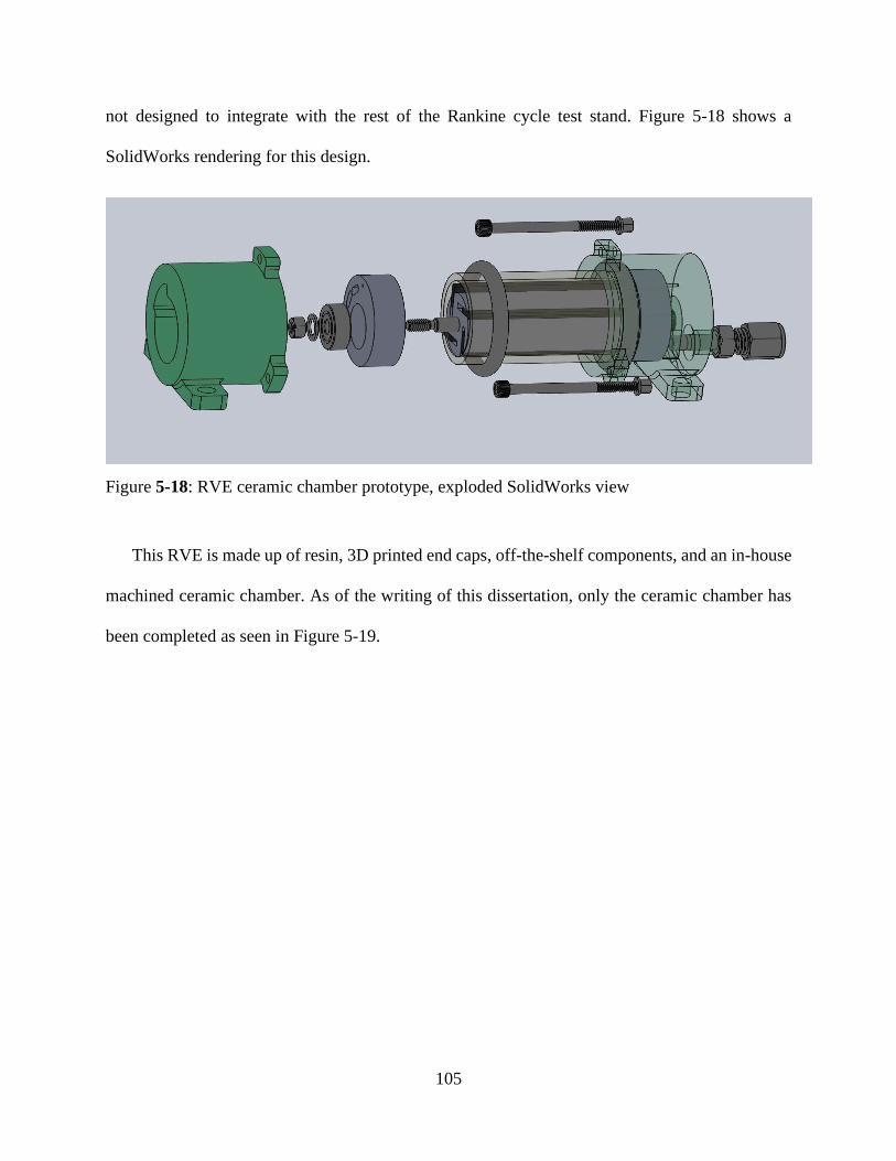
105
not designed to integrate with the rest of the Rankine cycle test stand. Figure 5-18 shows a
SolidWorks rendering for this design.
Figure 5-18: RVE ceramic chamber prototype, exploded SolidWorks view
This RVE is made up of resin, 3D printed end caps, off-the-shelf components, and an in-house
machined ceramic chamber. As of the writing of this dissertation, only the ceramic chamber has
been completed as seen in Figure 5-19.
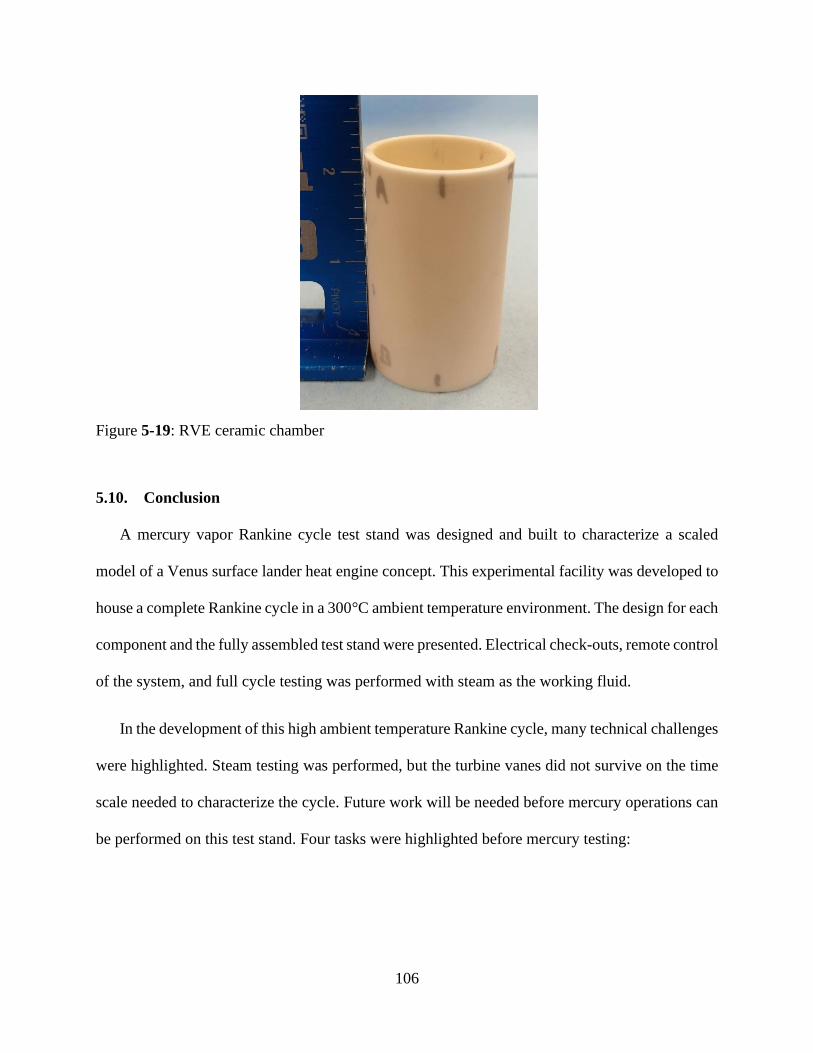
106
Figure 5-19: RVE ceramic chamber
5.10. Conclusion
A mercury vapor Rankine cycle test stand was designed and built to characterize a scaled
model of a Venus surface lander heat engine concept. This experimental facility was developed to
house a complete Rankine cycle in a 300°C ambient temperature environment. The design for each
component and the fully assembled test stand were presented. Electrical check-outs, remote control
of the system, and full cycle testing was performed with steam as the working fluid.
In the development of this high ambient temperature Rankine cycle, many technical challenges
were highlighted. Steam testing was performed, but the turbine vanes did not survive on the time
scale needed to characterize the cycle. Future work will be needed before mercury operations can
be performed on this test stand. Four tasks were highlighted before mercury testing:
107
1) The current air-cooled oil loop for the condenser is under-powered. Currently the oil loop
is being bypassed and an external chiller is attached to provide enough cooling. The
geometry of the condenser will be adjusted to increase the cooling surface area.
2) The rotary vane expander vanes are currently unable to perform long enough for a full test
if there is any condensation entering the expander. An alternative vane material will be
selected, and the turbine characterized for performance.
3) Alternatively, the quality of the gas entering the expander could be regulated. This can be
done by superheating the working fluid or installing a condensate trap after the evaporator.
Either of these changes would increase the quality of the gas being supplied to the
expander, potentially reducing the issue of wear on the vanes.
4) Validation of mercury testing procedures will be performed with Penn States EHS
department and the removal process verified.

108
Chapter 6
Conclusions and Recommendations for Future
Research
109
In this chapter, the major findings of this Ph.D. dissertation for the development of a metal
combustion power system are summarized. Then some recommendations are suggested for
continued development of this technology.
6.1. Lithium and carbon-dioxide, batch reactor modeling and experiments
In Chapters 2-3, modeling and experimental results are presented for lithium and carbon
dioxide batch reactors. A new detailed thermodynamic and heat transfer model of a conceptual
lithium combustion power system with an in-situ, carbon dioxide oxidizer was created. It found
an in-situ Li-CO2 powered Venus lander could supply 14 kWth of thermal energy for five days
with 185 kg of fuel. Even greater mission durations were determined if lower power missions are
considered. This model assumed complete and stoichiometric combustion of lithium and the
oxidizer. To characterize this further an experimental facility was built to test Li-CO2 batch
reactors.
In Chapter 3, five single-use Li-CO2 batch reactors were presented. These stainless-steel
vessels were each filled with solid lithium and then heated toward Venus surface temperatures,
which exceed the auto-ignition temperatures for combustion with carbon dioxide. Carbon dioxide
was metered into the reactors by a mass flow controller and the reaction rate was controlled to
regulate the temperature in the lithium bath to a specific value. It was determined from these
experiments that the lithium yield is a function of the reaction temperature. As the bath temperature
was increased, more of the lithium fuel was reacted with the available carbon dioxide. At lower
temperatures, a thick product crust formed over the molten Li, limiting fuel utilization. At ~900°C,
nearly all Li fuel was reacted (>98%), yielding a fuel-specific energy of 25.6 ± 0.7 MJ kgLi−1.
110
6.2. Mercury vapor Rankine cycle analysis and testing
In Chapters 4-5 a heat engine was selected for Venus surface conditions and the progress of
the experimental, cycle test stand was presented. In Chapter 4 the analysis and design of a viable
Venus surface heat engine was performed, and a mercury vapor Rankine cycle selected. It was
determined this cycle could power a future Venus lander if supplied 12.3 kW of thermal heat. With
that thermal energy it will provide 2.0 kW of shaft power to the spacecraft and perform with a
power efficiency of 16%. A scaled-down configuration was defined that can be assessed at
laboratory scale and a list of engineering requirements provided for a future mission enabled by
this technology.
In Chapter 5 the development of a high ambient temperature, mercury vapor Rankine cycle
test stand was presented. Each component was analyzed, their designs presented, and the test stand
presented. In the development of this cycle, many technical challenges were highlighted. Steam
testing was performed, but the turbine vanes did not survive on the time scale needed to
characterize the cycle. Future work will be needed before mercury operations can be performed.
An improved turbine design was presented, and test stand modifications suggested to achieve the
scaled-down configuration.
6.3. Recommendations for future research
More research studies are needed to extensively characterize metal-combustion fueled power
systems for extreme environment spacecraft. My recommendations for future work in this area
include:
111
1. Additional Li-CO2 experiments are needed to better understand how to achieve the best
specific energy for the batch reactors. Test should be performed to determine the “sweet
spot” between lithium utilization and specific energy by reaching the “third” stage of the
reaction process.
a. These experiments would benefit from improved insulation to better characterize
the heat of reaction and heat delivery system.
b. To achieve the higher specific energy expected from lower temperature reactions,
methods of agitation for batch reactors are recommended.
2. As the current Rankine cycle test stand is still in development my recommendation is for
continued component testing. Current off-the-shelf technologies do not exist for mercury
pressurization or expansion. To increase the maturity of the whole cycle, each component
needs to be tested and characterized for high temperature, mercury operation. Many
valuable challenges are being found and worked through with the current design, but
alternative pump and expander design testing would be valuable.
112
Bibliography
[1] M. Bullock, J.L. Hall, D.A. Senske, J.A. Cutts, R. Grammier, "Venus Flagship Study
Report," National Aeronautics and Space Administration, Jet Propulsion Laboratory,
Pasadena, California, 2009. https://doi.org/10.1073/pnas.0703993104.
[2] K. P. Hand, A. E. Murray, J. B. Garvin, and the Science Definition Team, “Report of the
Europa Lander Science Definition Team,” National Aeronautics and Space
Administration, Jet Propulsion Laboratory, Pasadena, California, JPL D-97667, 2017.
[3] E. S. Team, “Europa Study 2012 Report,” National Aeronautics and Space
Administration, Jet Propulsion Laboratory, Pasadena, California, JPL D-71990, 2012.
[4] National Research Council, Space Studies Board, "Vision and Voyages for Planetary
Science in the Decade 2013-2022," Washington DC, The National Academies Press,
2011. https://doi.org/https://doi.org/10.17226/13117.
[5] G. A. Landis and E. Haag, “Analysis of solar cell efficiency for Venus atmosphere and
surface missions,” in: 11th International Energy Conversion Engineering Conference, San
Jose, CA, 2013: pp. 1-9. https://doi.org/10.2514/6.2013-4028
[6] T.F. Miller, M. V. Paul, S.R. Oleson, "Combustion-based power source for Venus surface
missions," Acta Astronautica, Vol. 127, 2016. pp. 197–208.
https://doi.org/10.1016/j.actaastro.2016.05.006.
[7] S. Sell, Europa Lander Overview and Update, in: International Planetary Probe Workshop
2019, https://pub-lib.jpl.nasa.gov/docushare/dsweb/Get/Document-7094/01_Europa-
Lander-Overview-and-Update_SELL.pdf.
113
[8] J.F. Mondt, M.L. Underwood, B.J. Nesmith, "Future Radioisotope Power Needs for
Missions to the Solar System," in: 32nd Intersociety Energy Conversion Engineering
Conference, Honolulu, Hawaii, 1997: pp. 460–464.
[9] T. Baker, T.F. Miller, M. Paul, J.A. Peters, "The Use of Lithium Fuel with Planetary In
Situ Oxidizers," in: 10th Symposium on Space Resource Utilization, AIAA SciTech
Forum, Grapevine, Texas, 2017. pp. 1–11. https://doi.org/10.2514/6.2017-0650.
[10] R. Surmpudi, et al. "Energy Storage Technologies for Future Planetary Science Missions,"
JPL D-101146, Strategic Missions and Advanced Concepts Office Solar System
Exploration Directorate Jet Propulsion Laboratory, Pasadena, California, 2017.
https://solarsystem.nasa.gov/system/downloadable_items/716_Energy_Storage_Tech_Rep
ort_FINAL.PDF.
[11] L.S. Glaze, C.F. Wilson, L. V. Zasova, M. Nakamura, S. Limaye, "Future of Venus
Research and Exploration," Space Science Reviews Vol. 214, Issue 5, 2018. pp. 1-37.
https://doi.org/10.1007/s11214-018-0528-z.
[12] R. Lorenz, D. Mehoke, S. Hill, "Venus Pathfinder: A Stand-Alone Long-Lived Venus
Lander Mission Concept," Johns Hopkins University Applied Physics Laboratory, Laurel,
MD, 2012.
[13] G.A. Landis, "Robotic exploration of the surface and atmosphere of Venus," in: Acta
Astronautica, Vol. 59, Issue 7, 2006. pp. 570–579.
https://doi.org/10.1016/j.actaastro.2006.04.011.
[14] G.A. Landis, K.C. Mellott, "Venus surface power and cooling systems," in: Acta
Astronautica, Vol. 61, Issue 11-12, 2007. pp. 995–1001.
114
https://doi.org/10.1016/j.actaastro.2006.12.031.
[15] L. Balkanyi, G. Landis, et al., “COMPASS Final Report: Advanced Lithium Ion Venus
Explorer (ALIVE),” Glenn Research Center, NASA, Cleveland, Ohio, 2012.
[16] D.M. Hunten, L. Colin, T.M. Donahue, V.I. Moroz, "Venus," The University of Arizona
Press, Tuscan, AZ, 1983. ISBN 0-8165-0788-0
[17] E. Kolawa, et al., "Extreme Environments Technologies for Future Space Science
Missions," Report JPL D-32832, National Aeronautics and Space Administration, Jet
Propulsion Laboratory, Pasadena, California, 2007.
[18] L.A. Hennis, M.N. Varon, "Thermal Design and Development of Pioneer Venus Large
Probe," in: Thermophysics Heat Transfer Conference, Hughes Aircraft Company, El
Segundo, CA, 1978: pp. 425–445.
[19] K.R. Anderson, T. Gross, C. McNamara, A. Gatti, "Venus lander electronics payload
thermal management using a multistage refrigeration system," in Journal of
Thermophysics and Heat Transfer, Vol. 32, Issue 3, 2018. pp. 659–668.
https://doi.org/10.2514/1.T5286.
[20] Q.V. Nguyen, G.W. Hunter, "NASA High Operating Temperature Technology Program
Overview," in: 15th Meeting of the Venus Exploration Analysis Group (VEXAG), Laurel,
Maryland, U.S.A., 2017. https://doi.org/10.1111/1440-1681.12729.
[21] P.G. Neudeck, R.D. Meredith, L. Chen, D.J. Spry, L.M. Nakley, G.W. Hunter, "Prolonged
silicon carbide integrated circuit operation in Venus surface atmospheric conditions," in:
AIP Advances, Vol. 6, Issue 12, 2016. https://doi.org/10.1063/1.4973429.
115
[22] L. Chen, P.G. Neudeck, R.D. Meredith, D. Lukco, D.J. Spry, L.M. Nakley, K.G. Phillips,
G.M. Beheim, G.W. Hunter, "Sixty Earth-Days Test of a Prototype Pt/HTCC Alumina
Package in Simulated Venus Environment," in: Journal of Microelectronics and Electronic
Packaging, Vol. 16, No. 2, April 2019. pp. 78-83, https://doi.org/10.4071/imaps.873073
[23] K.R. Anderson, T.J. Gross, C. McNamara, A. Gatti, "Thermodynamic analysis of a
cascade refrigeration cycle for venus lander electronics cooling," in: Journal of
Thermophysics and Heat Transfer, Vol. 33, No. 3, September 2019. pp. 762–772.
https://doi.org/10.2514/1.T5571.
[24] R.W. Dyson, G.A. Bruder, "Progress Towards the Development of a Long-Lived Venus
Lander Duplex System," in: 46th AIAA/ASME/SAE/ASEE Joint Propulsion Conference
& Exhibit, Nashville, TN U.S.A., July 2010. https://doi.org/10.2514/6.2010-6917.
[25] K.D. Mellott, "Power conversion with a stirling cycle for venus surface mission," in: 2nd
International Energy Conversion Engineering Conference, Providence, RI, U.S.A., 2004.
https://doi.org/10.2514/6.2004-5622.
[26] R. Surampudi, J. Blosiu, P. Stella, J. Elliott, J. Castillo, T. Yi, J. Lyons, M. Piszczor, J.
Mcnatt, C. Taylor, S. Liu, E. Plichta, P.M. Beauchamp, J.A. Cutts, "Solar Power
Technologies for Future Planetary Science Missions," JPL D-101316, Pasadena,
California, 2017. https://solarsystem.nasa.gov.
[27] J. Grandidier, A.P. Kirk, M.L. Osowski, P.K. Gogna, S. Fan, M.L. Lee, M.A. Stevens, P.
Jahelka, G. Tagliabue, H.A. Atwater, J.A. Cutts, "Low-Intensity High-Temperature
(LIHT) Solar Cells for Venus Atmosphere," in: IEEE Journal of Photovoltaics, Vol. 8,
Issue 6, 2018. pp. 1621–1626. https://doi.org/10.1109/JPHOTOV.2018.2871333.
116
[28] M. Bugga, Ratnakumar V. Jones, John-Paul Pauken, K.J. Billings, S.A. Stariha, C. Ahn,
B. Fultz, K. Nock, J. Cutts, "New Power Technology for Venus Aerial Missions," The
Electrochemical Society Meeting Abstracts, 2019.
[29] R. Bugga, J. Jones, M. Pauken, E. Brandon, C. Ahn, B. Fultz, "Electrochemical Power
Sources for Venus Exploration," in: KISS Workshop, Caltech, Pasadena, California, 2017.
pp. 1-13
[30] S.A. Stariha, K.J. Billings, J.-P. Jones, R. Bugga, "Regenerative Solid Oxide Fuel Cells
for Venus Interior Probe Energy Storage," The Electrochemical Society Meeting
Abstracts, 2019.
[31] T.G. Hughes, R.B. Smith, D.H. Kiely, "Stored Chemical Energy Propulsion System for
Underwater Applications," in: AIAA/SAE/ASME 17th Joint Propulsion Conference,
Colorado Springs, Colorado, 1982. pp. 128–133.
[32] J. Gilchrist, B. Ayers, L. Parnell, "Heat transfer distribution in closed liquid metal
combustion - Effects of combustion products," in: AIAA/SAE/ASME/ASEE 29th Joint
Propulsion Conference and Exhibit, Monterey, CA, 1993. https://doi.org/10.2514/6.1993-
2205.
[33] K.-Y. Hsu, L.-D. Chen, "An experimental study of Li-SF6 wick combustion and
morphology analysis of combustion products," in: AIAA/SAE/ASME/ASEE 27th Joint
Propulsion Conference, Sacramento, CA, 1991. https://doi.org/10.2514/6.1991-2447.
[34] C. Tarau, M. DeChristopher, W.G. Anderson, "Diode heat pipes for Long-lived Venus
Landers," in: 10th Annual International Energy Conversion Engineering Conference
IECEC, Atlanta, Georgia, 2012: pp. 1–11. https://doi.org/10.2514/6.2012-3893.
117
[35] E. Shafirovich, A. Varma, "Metal-CO2 Propulsion for Mars Missions: Current Status and
Opportunities," in: Journal Propulsion and Power. Vol. 24, Issue 3, 2008. pp. 385–394.
https://doi.org/10.2514/1.32635.
[36] R.A. Rhein, "The Utilization of Powered Metals as Fuels in the Atmospheres of Venus,
Earth, and Mars," Report 32-1073, NASA Jet Propulsion Laboratory, Pasadena,
California, 1967.
[37] R. Zubrin, T. Muscatello, B. Birnbaum, K. Caviezel, G. Snyder, M. Berggren, "Progress
in Mars ISRU technology," in: 40th AlAA Aerospace Sciences Meeting and Exhibit,
Reno, NV, January 2002: pp.1-15. https://doi.org/10.2514/6.2002-461.
[38] S. Yuasa, H. Isoda, "Carbon dioxide breathing propulsion for a Mars airplane," in: 25th
Joint Propulsion Conference, Monterey, CA, 1989: pp.1-7. https://doi.org/10.2514/6.1989-
2863.
[39] R.W. Dyson, G.A. Bruder, "Progress towards the development of a long-lived Venus
lander duplex system," in: 8th Annual International Energy Conversion Engineering
Conference, Nashville, TN, 2010. pp.1–11. https://doi.org/10.2514/6.2010-6917.
[40] M.A. Frerking, P.M. Beauchamp, "JPL technology readiness assessment guideline," IEEE
Aerospace Conference, Big Sky, MT, 2016. https://doi.org/10.1109/AERO.2016.7500924.
[41] S. Yuasa, H. Isoda, "Ignition and Combustion of Metals in a Carbon Dioxide Stream," in:
Twenty-Second Symposium (International) on Combustion, The Combustion Institute,
Vol 22, Issue 1, 1989. pp. 1635–1641. https://doi.org/10.1016/S0082-0784(89)80175-4
[42] S.A. Klein, EES – Engineering Equation Solver, Version 10.643-3D (2019-05-52),
118
(2019). http://fchartsoftware.com.
[43] C.Y. Ho, T.K. Chu, "Electrical resistivity and thermal conductivity of nine selected AISI
stainless steels," Cindas Report 45, Purdue University, 1977.
[44] R. Span, W. Wagner, "A New Equation of State for Carbon Dioxide Covering the Fluid
Region from the Triple- Point Temperature to 1100 K at Pressures up to 800 MPa," in
Journal of Physical and Chemical Reference Data, Vol. 25, Issue 6, 1996. pp.1509–1596.
https://doi.org/10.1063/1.555991.
[45] Mikron Instrument Company, "Table of Emissivity of Various Surfaces," 2014, pp. 1–13.
https://doi.org/http://www-
eng.lbl.gov/~dw/projects/DW4229_LHC_detector_analysis/calculations/emissivity2.pdf.
[46] J.K. Fink, L. Leibowitz, "Thermodynamic and Transport Properties of Sodium Liquid and
Vapor," Report ANL/RE-95/2, Argonne National Laboratory, Illinois, 1995. pp. 1–238.
https://doi.org/10.2172/94649.
[47] N.B. Vargaftik, Y.S. Touloukian, "Handbook of Physical Properties of Liquids and
Gases," Hemisphere Publishing Corporation VI, 1996. pp. 1-1370. ISBN: 3-540-16972-5
[48] R. Span, W. Wagner, "Equations of State for Technical Applications. II. Results for
Nonpolar Fluids," in: International Journal of Thermophysics, Vol. 24, No.1, January
2003. pp. 41–109. https://doi.org/10.1023/A:1022310214958.
[49] W.A. Cole, K.M. de Reuck, "An interim analytic equation of state for sulfurhexafluoride,"
in: International Journal of Thermophysics, Vol. 11, Issue 1, 1990. pp. 189–199.
https://doi.org/10.1007/BF00503870.
119
[50] N.- JANAF, NIST - JANAF Thermochemical Tables, Natl. Inst. Stand. Technol. (2016).
http://kinetics.nist.gov/janaf.
[51] Faghri A., Y. Zhang, "Transport phenomena in Multiphase Systems," Elsevier Academic
Press, 2006. pp. 1-1030. ISBN: 9780123706102. https://doi.org/10.1016/B978-0-12-
370610-2.50010-6.
[52] M.N. Ivanovskii, V.P. Sorokin, I.V. Yagodkin, "The physical principles of heat pipes,"
Oxford University Press, New York, 1982. pp.1-262. ISBN: 0198514662
[53] B.J. McBride, M.J. Zehe, S. Gordon, "NASA Glenn Coefficients for Calculating
Thermodynamic Properties of Individual Species," Report TP-2002-211556, NASA Glenn
Research Center, Cleveland, Ohio, 2002. pp. 291. https://doi.org/NASA/TP—2002-
211556.
[54] I.A. Zelenov, A.F. Klishin, A.F. Shabarchin, "Thermal protection and test method of
“VENERA” landing spacecrafts," in: European Conference on Spacecraft Structures,
Materials & Mechanical Testing, Noordwijk, The Netherlands, ESA SP-581, 2005. pp.
789–795.
[55] R.D. Lorenz, B. Bienstock, P. Couzin, G. Cluzet, "Thermal design and performance of
probes in thick atmospheres: experience of Pioneer Venus, Venera, Galileo and Huygens,"
in: 3rd International Planetary Probe Workshop, Athens, Greece, 2005.
[56] S.W. Churchill, M. Bernstein, "A Correlating Equation for Forced Convection From
Gases and Liquids to a Circular Cylinder in Crossflow," in: Journal of Heat Transfer, Vol.
99, May 1977. pp. 300-306. https://doi.org/10.1115/1.3450685.
120
[57] R.E. Arvidson, V.R. Baker, C. Elachi, R.S. Saunders, J.A. Wood, "Magellan: Initial
Analysis of Venus Surface Modification," in: Science, Vol.252, Issue 5003, 1991. pp.
270–275. https://doi.org/10.1126/science.252.5003.270.
[58] L.V. Ksanfomaliti, N.V. Goroshkova, V.K. Khondyrev, "Wind velocity at the Venus
surface according to acoustic measurements," in: Kosmicheskie Issledovaniia, Vol. 21 ,
1983. pp. 218–224.
[59] A. Jasmin Sudha, K. Velusamy, "Numerical analysis of natural convection in sodium
plenum below the grid plate of a fast reactor during a severe accident," in: Annals Nuclear
Energy, Vol. 54, 2013. pp. 120–128. https://doi.org/10.1016/j.anucene.2012.11.004.
[60] R.C. Noyes, "An experimental study of sodium pool boiling heat transfer," in: Journal of
Heat Transfer, May 1963. pp. 1–6.
[61] J. Yang, F.R. Stabler, "Automotive applications of thermoelectric materials," in: Journal
of Electronic Materials, Vol. 38, No. 7, 2009. pp. 1245–1251.
https://doi.org/10.1007/s11664-009-0680-z.
[62] J. Yang, T. Caillat, "Thermoelectric Materials for Space," in: MRS Bulletin, Vol. 31,
March 2006. pp. 224–229.
[63] NASA, "Advanced Stirling Radioisotope Generator," in: NASA Facts. NF-2013-07-568-
HQ, 2013. pp. 2. https://solarsystem.nasa.gov/rps/docs/APP ASRG Fact Sheet v3 9-3-
13.pdf (accessed January 1, 2017).
[64] T.H. Kwan, X. Wu, "Power and mass optimization of the hybrid solar panel and
thermoelectric generators," in: Applied Energy, Vol. 165, 2016. pp. 297–307.
121
https://doi.org/10.1016/j.apenergy.2015.12.016.
[65] P. Fischer, M. Schiemann, V. Scherer, G. Schmid, D. Taroata, "Experimental study on the
combustion of Lithium particles in CO2 and CO2-N2 mixtures," in: Fuel. Vol. 102, 2012.
pp. 431–438. https://doi.org/10.13140/RG.2.1.1906.8968
[66] T.E. Little, "Reactivity of Nitrogen, Oxygen, and Halogenated Gases with Molten Lithium
Metal," No. TM-72-232, The Pennsylvania State University, 1973.
[67] D. Lukco, D.J. Spry, R.P. Harvey, G.C.C. Costa, R.S. Okojie, A. Avishai, L.M. Nakley,
"Chemical Analysis of Materials Exposed to Venus Temperature and Surface
Atmosphere," in: Earth and Space Science, Vol. 5, Issue 7, 2018. pp. 270–284.
https://doi.org/10.1029/2017EA000355.
[68] C. Greer, A. Rattner, Experimental Lithium Facility Repository, PennState Sch. (2020).
https://scholarsphere.psu.edu/concern/generic_works/vt435gf45w (accessed August 6,
2020).
[69] E.G. Groff, G.M. Faeth, "Steady Metal Combustor as a Closed Thermal Energy Source,"
in: Journal of Hydronautics, Vol. 12, No 2. April 1978. pp. 63–70.
[70] S.J. Conway, J. Szanyi, J.H. Lunsford, "Catalytic properties of lithium carbonate melts
and related slurries for the oxidative dimerization of methane," in: Applied Catalysis, Vol.
56, Issue 1, 1989. pp. 149–161. https://doi.org/10.1016/S0166-9834(00)80165-7.
[71] NIST-JANAF, "NIST-JANAF Thermochemical Tables: Li2CO3," National Institute of
Standards and Technology, (1966). [Online]. https://doi.org/10.18434/T42S31.
[72] A. Kozlov, M. Seyring, M. Drüe, M. Rettenmayr, R. Schmid-fetzer, "The Li – C phase
122
equilibria," in: International Journal of Materials Research, Vol. 104, Issue 11, 2013. pp.
1066–1078. https://doi.org/https://doi.org/10.3139/146.110960.
[73] R.M. Yonco, V.A. Maroni, J.E. Strain, J.H. Devan, "A determination of the solubility of
lithium oxide in liquid lithium by fast neutron activation," in: Journal of Nuclear
Materials, Vol. 79, Issue 2, 1979. pp. 354–362. https://doi.org/10.1016/0022-
3115(79)90100-4.
[74] R.M. Yonco, M.I. Homa, "The solubility of carbon in low-nitrogen liquid lithium," in:
Journal of Nuclear Materials, Vol. 138, Issue 1, 1986. pp. 117–122.
https://doi.org/10.1016/0022-3115(86)90262-X.
[75] K.Y. Hsu, L.D. Chen, "An experimental investigation of Li and SF6 wick combustion,"
in: Combustion and Flame, Vol. 102, Issue 1-2, 1995. pp. 73–86.
https://doi.org/10.1016/0010-2180(94)00238-N.
[76] B.B. Alchagirov, L.K. Afaunova, F.F. Dyshekova, A.G. Mozgovoi, T.M. Taova, R.K.
Arkhestov, "The density and surface tension of liquid lithium at melting temperature," in:
High Temperature, Vol. 47, Issue 2, 2009. pp. 287–291.
https://doi.org/10.1134/S0018151X09020205.
[77] P. Fiflis, A. Press, W. Xu, D. Andruczyk, D. Curreli, D.N. Ruzic, "Wetting properties of
liquid lithium on select fusion relevant surfaces," in: Fusion Engineering and Design, Vol.
89, Issue 12, 2014. pp. 2827–2832. https://doi.org/10.1016/j.fusengdes.2014.03.060.
[78] C. Ahrens, James, Geveci, Berk, Law, "ParaView: An End-User Tool for Large Data
Visualization," in: Visualization Handbook, Elsevier, 2005. ISBN: 978-0123875822
123
[79] M.G. Ktalkherman, V.A. Emelkin, B.A. Pozdnyakov, "Production of lithium oxide by
decompostion lithium carbonate in the flow of a heat carrier," in: Theoretical Foundations
of Chemical Engineering, Vol. 43, Issue 1, 2009. pp. 88–93.
https://doi.org/10.1134/S0040579509010114.
[80] C.J. Greer, M.V. Paul, A.S. Rattner, "Analysis of lithium-combustion power systems for
extreme environment spacecraft," in: Acta Astronautica, Vol. 151, 2018. pp. 68–79.
https://doi.org/10.1016/j.actaastro.2018.05.039.
[81] R.W. Dyson, P.G. Schmitz, L.B. Penswick, G.A. Bruder, "Long-lived Venus lander
conceptual design: How to keep it cool," in: 7th International Energy Conversion
Engineering Conference, Devner, Colorado, 2009. https://doi.org/10.2514/6.2009-4631.
[82] T. Kremic, G.W. Hunter, L. Nero, "Long-Lived In-Situ Solar System Explorer (LLISSE),"
in: Venera-D Modeling Workshop, Moscow, Russia, 2017. pp. 1–5.
[83] TEC Solid State Power Generators, "CMO-32-62S Datasheet" (accessed April 6, 2020).
https://thermoelectric-generator.com/wp-content/uploads/2014/04/CMO-32-62S-OXIDE-
ONLY-new.pdf
[84] L.M. Fraas, J.E. Avery, H.X. Huang, "Thermophotovoltaics: heat and electric power from
low bandgap “solar” cells around gas fired radiant tube burners, in: IEEE Photovolt. Spec.
Conf., New Orleans, LA, 2002. pp. 1553-1556.
https://doi.org/10.1109/PVSC.2002.1190909.
[85] Z. Zhou, X. Sun, P. Bermel, "Radiative cooling for thermophotovoltaic systems," in: SPIE
Optical Engineering + Applications, Infrared Remote Sensing and Instrumentation XXIV,
997308, San Diego, CA, Vol. 9973, 2016. https://doi.org/10.1117/12.2236174
124
[86] V.P. Khvostikov, S. V Sorokina, N.S. Potapovich, F.Y. Soldatenkov, N.K. Timoshina,
"Temperature stability of contact systems for GaSB-based photovoltaic converters," in:
Semiconductors, Vol. 48, No.9, 2014. pp. 1248–1253.
https://doi.org/10.1134/S1063782614090115
[87] K. Anderson, T. Gross, C. McNamara, A. Gatti, "Design and analysis of a FAME-MLL
vapor-compression refrigeration cycle compressor," in: Thermal Fluid Engineering
Conference, Las Vegas, NV, 2019. pp. 1593-1602.
https://doi.org/10.1615/TFEC2019.ref.026265
[88] E. Mumm, Honeybee Robotics, "High temperature motor extreme environment actuator,"
(accessed April, 2020), https://honeybeerobotics.com/wp-
content/uploads/2014/07/Honeybee-Robotics-High-Temperature-Motor.pdf
[89] S. Oriti, S. Wilson, M. Hickman, J. Zakrejsek, "Dynamic radioisotope power systems
development and potential first mission utilization," NASA Glenn Research Center,
Cleveland, Ohio, 2018. (accessed, July, 2020)
https://ntrs.nasa.gov/archive/nasa/casi.ntrs.nasa.gov/20180005489.pdf
[90] S. Wilson, S. Oriti, "Maturation of dynamic power converters for radioisotope power
systems," in: Nuclear and Emerging Technologies for Space, American Nuclear Society
Topical Meeting, Richland, WA, 2019.
[91] J.P. Stone, C.L. Wing, J.R. Spann, E.W. Steinkuller, D.D. Williams, R.R. Miller, "High
Temperature Vapor Pressures of Sodium, Potassium, and Cesium," Journal of Chemical
and Engineering Data, Vol. 11, Issue 3, 1966. pp. 315–320.
https://doi.org/10.1021/je60030a007.
125
[92] M. Gutstein, E.R. Furman, G.M. Kaplan, "Liquid-Metal Binary Cycles for Stationary
Power," NASA Report TN D-7955, Lewis Research Center, August 1975.
[93] P. Bombarda, C. Invernizzi, "Binary liquid metal–organic Rankine cycle for small power
distributed high efficiency systems,"in: Journal of Power and Energy, Vol. 229, Issue 2,
2015. pp. 192–209. https://doi.org/10.1177/0957650914562094.
[94] A. Fox, J.F. Louis, W.J. Greenlee, G.H. Parker, "Binary Mercury/Organic Rankine Cycle
Power Systems," in: 22nd Intersociety Energy Conversion Engineering Conference,
Reston, Virginia, 1987. pp. 127–132. https://doi.org/10.2514/6.1987-9162.
[95] W.R. Chambers, A.P. Fraas, M.N. Ozisik, "A Potassium-Steam Binary Vapor Cycle for
Nuclear Power Plants," Report ORNL-3584, Oak Ridge, Tennessee, May 1964.
[96] J.M. Bergthorson, S. Goroshin, M.J. Soo, P. Julien, J. Palecka, D.L. Frost, D.J. Jarvis,
"Direct combustion of recyclable metal fuels for zero-carbon heat and power," in: Applied
Energy, Vol. 160, 2015. pp. 368–382. https://doi.org/10.1016/j.apenergy.2015.09.037.
[97] L. Rosenblum, "Liquid Metals For Aerospace Electric-Power Systems," in: Journal of
Metals, Vol. 637, September 1963. pp. 637–641. https://doi.org/10.1007/BF03397240
[98] D.R. Snoke, G.L. Mrava, "Silent Mercury Rankine Cycle Power System," in: Society of
Automotive Engineers Summer Meeting, Chicago, Illinois, 1964. pp. 10.
https://doi.org/10.4271/640266
[99] H.C. Young, A.G. Grindell, "Summary of Design and Test Experience With Cesium and
Potassium Components and Systems For Space Power Plants," Report ORNL-TM-1833,
Oak Ridge National Laboratory, TN, 1967.
126
[100] N.L. Zhang, D.F. Chao, J.M. Sankovic, J.B. McQuillen, J.F. Lekan, :On analog simulation
of liquid-metal flows in space Rankine-cycle power-systems," in: ASME 2005
International Mechanical Engineering Congress and Exposition, Vol. 261, 2005. pp. 755-
761. https://doi.org/10.1115/IMECE2005-81307.
[101] G.L. Yoder, R.L. Graves, "Analysis of Alkali Liquid Metal Rankine Space Power
Systems," in: 2nd Nuclear Space Power Symposium, Albuquerque, NM, 1985.
[102] G. Yoder, J. Carbajo, R. Murphy, A. Qualls, J. Hojnicki, M. Moriarty, F. Widman, K.
Metcalf, M. Nikitkin, "Potassium Rankine Cycle System Design Study for Space Nuclear
Electric Propulsion," in: 3rd International Energy Conversion Engineering Conference,
San Francisco, CA, 2005. https://doi.org/10.2514/6.2005-5637.
[103] F.W. Moffitt, Thomas P. and Klag, "Analytical Investigation of Cycle Characteristics For
Advanced Turboelectric Space Power Systems," Technical Note D-472, Lewis Research
Center, Cleveland, Ohio, 1960.
[104] L.S. Mason, "Power technology options for nuclear electric propulsion," in: 37th
Intersociety Energy Conversion Engineering Conference, Washington, DC, 2002. pp.
114–121. https://doi.org/10.1109/IECEC.2002.1391989
[105] R.T. Lahey, V. Dhir, "Research in Support of the Use of Rankine Cycle Energy
Conversion Systems for Space Power and Propulsion," NASA Glenn Research Center
Contractor Report CR-2004-213142, 2004.
[106] J.N. Hodgson, "Experimental investigation of the SNAP-8 mercury Rankine-cycle power
conversion system," NASA Topical Report CR-72679, Aerojet-General Corporation,
1969.
127
[107] Bobkov, V., L. Fokin, E. Petrov, V. Popov, V. Rumiantsev, and A. Savvatimsky,
"Thermophysical Properties of Materials for Nuclear Engineering: A Tutorial and
Collection of Data," International Atomic Energy Agency, Vienna, 2008
[108] Z. Gnutek, P. Kolasinski, "The application of rotary vane expanders in organic rankine
cycle systems - Thermodynamic description and experimental results," in Journal of
Engineering for Gas Turbines and Power, Vol. 135, 2013.
https://doi.org/10.1115/1.4023534.
[109] K.E. Nichols, "How to select turbomachinery for your application," Barber-Nichols Inc.
2020. (accessed April 2020)
http://www.costanteinvernizzi.it/Site_1/Downlodable_Documents_14_files/how_to_select
_turbomachinery_for_your_application.pdf
[110] P. Kolasiński, P. Blasiak, J. Rak, "Experimental and numerical analyses on the rotary vane
expander operating conditions in a micro organic rankine cycle system," in: Energies, Vol.
9, Issue 606, 2016. https://doi.org/10.3390/en9080606.
[111] R.J. Moffat, "Describing the Uncertainties in Experimental Results," in: Experimental
Thermal and Fluid Sciences, Vol. 1, 1988. pp. 3–17. https://doi.org/10.1016/0894-
1777(88)90043-X.
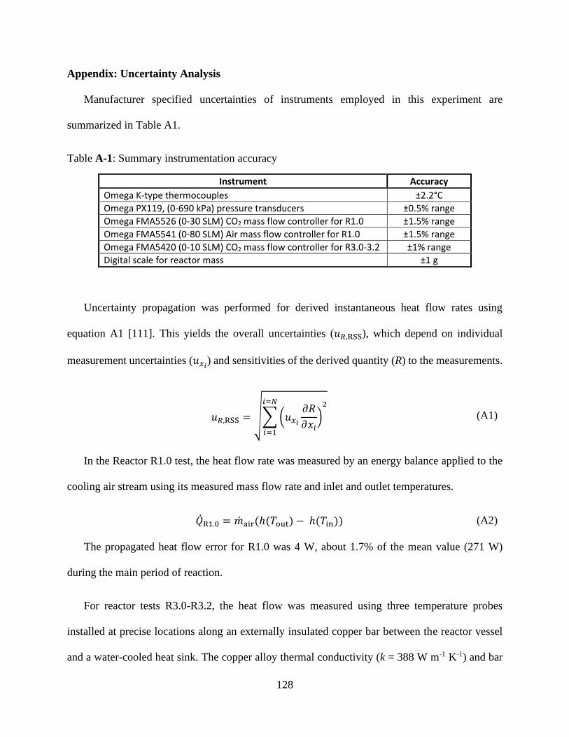
128
Appendix: Uncertainty Analysis
Manufacturer specified uncertainties of instruments employed in this experiment are
summarized in Table A1.
Table A-1: Summary instrumentation accuracy
Instrument Accuracy
Omega K-type thermocouples ±2.2°C
Omega PX119, (0-690 kPa) pressure transducers ±0.5% range
Omega FMA5526 (0-30 SLM) CO2 mass flow controller for R1.0 ±1.5% range
Omega FMA5541 (0-80 SLM) Air mass flow controller for R1.0 ±1.5% range
Omega FMA5420 (0-10 SLM) CO2 mass flow controller for R3.0-3.2 ±1% range
Digital scale for reactor mass ±1 g
Uncertainty propagation was performed for derived instantaneous heat flow rates using
equation A1 [111]. This yields the overall uncertainties (𝑢𝑅,RSS), which depend on individual
measurement uncertainties (𝑢𝑥𝑖) and sensitivities of the derived quantity (R) to the measurements.
𝑢𝑅,RSS = √∑ (𝑢𝑥𝑖
𝜕𝑅
𝜕𝑥𝑖)
2𝑖=𝑁
𝑖=1
(A1)
In the Reactor R1.0 test, the heat flow rate was measured by an energy balance applied to the
cooling air stream using its measured mass flow rate and inlet and outlet temperatures.
��R1.0 = ��air(ℎ(𝑇out) − ℎ(𝑇in)) (A2)
The propagated heat flow error for R1.0 was 4 W, about 1.7% of the mean value (271 W)
during the main period of reaction.
For reactor tests R3.0-R3.2, the heat flow was measured using three temperature probes
installed at precise locations along an externally insulated copper bar between the reactor vessel
and a water-cooled heat sink. The copper alloy thermal conductivity (k = 388 W m-1 K-1) and bar
129
cross-section area (A = 129 mm2) were known precisely. Therefore, heat flow uncertainties are
due to uncertainties in temperature measurements (±2.2°C) and spacing between thermocouples
(∆𝑥 = 32 ±1 mm).
Qwater−cooled =kA
2(
(Tx1 − Tx2)
(x1 − x2)+
(Tx2 − Tx3)
(x2 − x3)) (A3)
Uncertainties in unreacted lithium volume were estimated by repeating the analysis procedure
detailed in Section 3.4.1 with the threshold intensity value for distinguishing products from fuel
adjusted by ±10% of the baseline value. The greater of the deviations from the baseline for these
two values is reported as the uncertainty range. For example, for the R1.0 test, the baseline
utilization was found to be 41.9%. Adjusting the threshold +10% and -10% yielded utilizations of
45.8% (+3.9%) and 37.5% (-4.4%), respectively. Therefore, a conservative uncertainty of ±4.4%
was reported. It should be cautioned that the uncertainties for fuel utilization are based on heuristics
and are mainly intended to represent the likely range of values.
For the reaction tests, collected data could only specify final composition to within one degree
of freedom. This leads to wide ranges of possible reaction paths for some tests. For example, in
test R1.0, reaction 2 (Li2C2 oxidation) could have completed between 0% < f2 < 100%, and reaction
3 (Li2O oxidation) between 45 < f3 < 100%. Given these ranges, the linearized approach (Eqn. A1)
is unsuitable for estimating uncertainties in fuel-specific energy based on initial and final
compositions (qLi, qLi,reacted). Instead, a Monte Carlo procedure was performed. In this approach
specific energy was calculated using randomized sets of values of initial Li mass, added CO2 mass,
and Li utilization from within the uncertainty bands for those quantities. For each set a random
value of f2 (0 – 100%) was selected. Unphysical input sets that caused f3 < 0% or f3 > 100% were
discarded. 100 physical sets were averaged for each test to define the mean values for fuel-specific
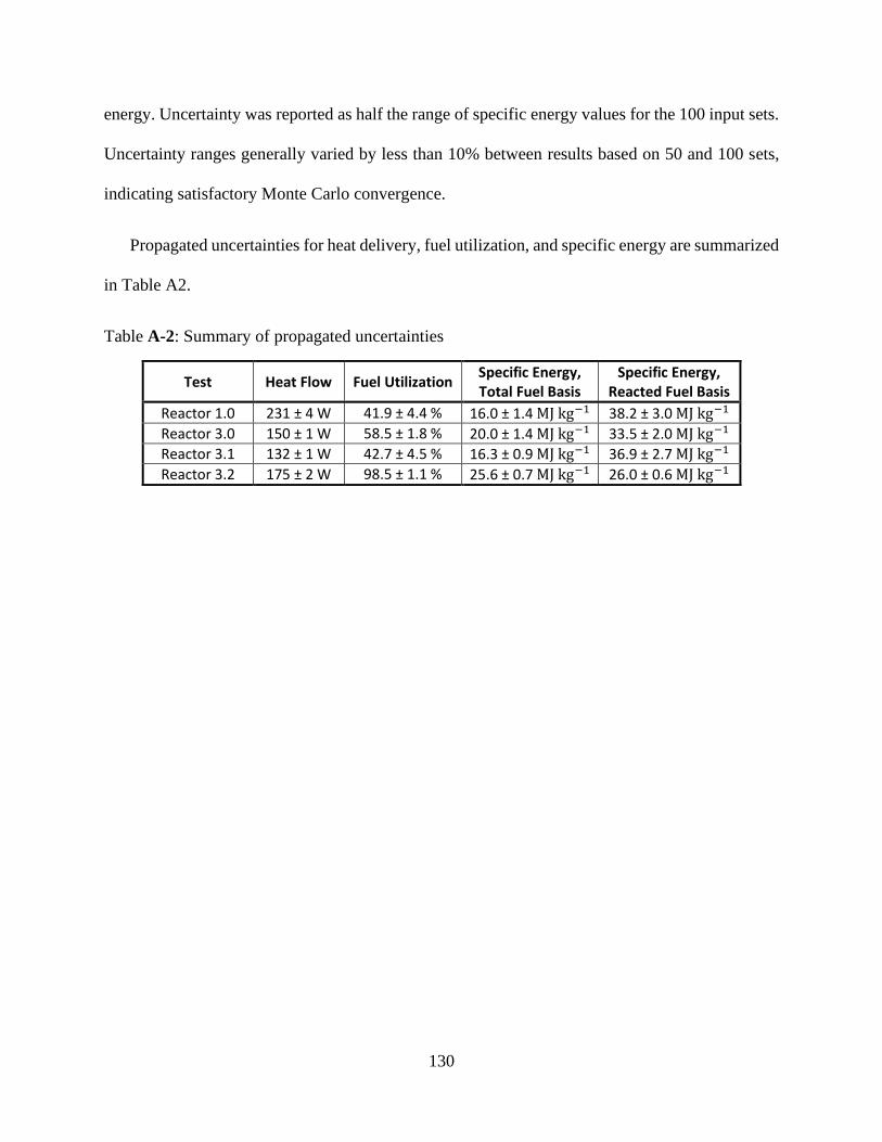
130
energy. Uncertainty was reported as half the range of specific energy values for the 100 input sets.
Uncertainty ranges generally varied by less than 10% between results based on 50 and 100 sets,
indicating satisfactory Monte Carlo convergence.
Propagated uncertainties for heat delivery, fuel utilization, and specific energy are summarized
in Table A2.
Table A-2: Summary of propagated uncertainties
Test Heat Flow Fuel Utilization Specific Energy, Total Fuel Basis
Specific Energy, Reacted Fuel Basis
Reactor 1.0 231 ± 4 W 41.9 ± 4.4 % 16.0 ± 1.4 MJ kg−1 38.2 ± 3.0 MJ kg−1
Reactor 3.0 150 ± 1 W 58.5 ± 1.8 % 20.0 ± 1.4 MJ kg−1 33.5 ± 2.0 MJ kg−1
Reactor 3.1 132 ± 1 W 42.7 ± 4.5 % 16.3 ± 0.9 MJ kg−1 36.9 ± 2.7 MJ kg−1
Reactor 3.2 175 ± 2 W 98.5 ± 1.1 % 25.6 ± 0.7 MJ kg−1 26.0 ± 0.6 MJ kg−1
131
VITA
Christopher J. Greer
Education
Ph.D., Mechanical Engineering, The Pennsylvania State University, University Park, PA May. 2021
M.Sc., Mechanical Engineering, The Pennsylvania State University, University Park, PA Dec. 2017
B.Sc., Mechanical Engineering, The Pennsylvania State University, University Park, PA Dec. 2015
Work Experience
Research Assistant, The Pennsylvania State University, University Park, PA Aug. 2015 – Dec. 2020
Ground Support Equipment Engineer, SpaceX, Hawthorne, CA Sep. 2014 – Dec. 2014
May. 2015 – Aug. 2015
Selected Publications
1. Acta Astronautica, https://doi.org/10.1016/j.actaastro.2018.05.039 C. J. Greer, M. V. Paul,
and A. S. Rattner, “Analysis of lithium-combustion power systems for extreme environment
spacecraft,” Acta Astronautica, vol. 151, no. May, pp. 68–79, 2018.
2. Acta Astronautica, https://doi.org/10.1016/j.actaastro.2021.01.010 C. J. Greer, J. A. Peters,
M. P. Manahan, J. J. Cor, and A. S. Rattner, “Experimental characterization of lithium-
carbon dioxide combustion in batch reactorsfor powering Venus landers,” Acta Astronautica,
available online Janurary 2021, in press, journal pre-proof.
Conference Presentations
1. IPPW-13 (International Planetary Probe Workshop) 2016, Applied Physics Laboratory,
Laurel MD • Venus Short Course Attendee and Workshop Student Presenter
2. IPPW-14 2017, The Hague, Netherlands • Ocean Worlds Short Course Attendee and
Workshop Student Presenter
3. IPPW-15 2018, CU Boulder, Boulder CO • Cube-Satellite Short Course Attendee and
Workshop Student Presenter
4. IPPW-16 2019, Oxford, United Kingdom • Ice Giants Short Course Attendee and Workshop
Student Presenter