Chemical Engineering Thermodynamics - Tufts UniversityMEASURED THERMODYNAMIC PROPERTIES AND OTHER BASIC CONCEPTS | 5 1. MEASURED THERMODYNAMIC PROPERTIES AND OTHER BASIC CONCEPTS 1.1

CHEMICAL ENGINEERING

THERMODYNAMICS Andrew S. Rosen

SYMBOL DICTIONARY | 1

TABLE OF CONTENTS Symbol Dictionary ........................................................................................................................ 3 1. Measured Thermodynamic Properties and Other Basic Concepts .................................. 5

1.1 Preliminary Concepts – The Language of Thermodynamics ........................................................ 5 1.2 Measured Thermodynamic Properties .......................................................................................... 5

1.2.1 Volume .................................................................................................................................................... 5 1.2.2 Temperature ............................................................................................................................................. 5 1.2.3 Pressure .................................................................................................................................................... 6

1.3 Equilibrium ................................................................................................................................... 7 1.3.1 Fundamental Definitions .......................................................................................................................... 7 1.3.2 Independent and Dependent Thermodynamic Properties ........................................................................ 7 1.3.3 Phases ...................................................................................................................................................... 8

2 The First Law of Thermodynamics ..................................................................................... 8 2.1 Definition of the First Law............................................................................................................ 8 2.2 Fundamental Definitions ............................................................................................................... 9 2.3 Work ............................................................................................................................................. 9 2.4 Hypothetical Paths ........................................................................................................................ 9 2.5 Reversible and Irreversible Processes ......................................................................................... 10 2.6 Closed Systems ........................................................................................................................... 10

2.6.1 Integral Balance ..................................................................................................................................... 10 2.6.2 Differential Balance ............................................................................................................................... 11

2.7 Isolated Systems .......................................................................................................................... 11 2.8 Open Systems .............................................................................................................................. 11 2.9 Open-System Energy Balance on Process Equipment ................................................................ 12

2.9.1 Introduction............................................................................................................................................ 12 2.9.2 Nozzles and Diffusers ............................................................................................................................ 13 2.9.3 Turbines and Pumps............................................................................................................................... 13 2.9.4 Heat Exchangers .................................................................................................................................... 13 2.9.5 Throttling Devices ................................................................................................................................. 13

2.10 Thermodynamic Data for 𝑈 and 𝐻 ............................................................................................. 13 2.10.1 Heat Capacity .................................................................................................................................... 13 2.10.2 Latent Heat ........................................................................................................................................ 14 2.10.3 Enthalpy of Reaction ......................................................................................................................... 14

2.11 Calculating First-Law Quantities in Closed Systems .................................................................. 15 2.11.1 Starting Point ..................................................................................................................................... 15 2.11.2 Reversible, Isobaric Process .............................................................................................................. 16 2.11.3 Reversible, Isochoric Process ............................................................................................................ 16 2.11.4 Reversible, Isothermal Process .......................................................................................................... 16 2.11.5 Reversible, Adiabatic Process ........................................................................................................... 16 2.11.6 Irreversible, Adiabatic Expansion into a Vacuum ............................................................................. 17

2.12 Thermodynamic Cycles and the Carnot Cycle............................................................................ 17 3 Entropy and the Second Law of Thermodynamics .......................................................... 18

3.1 Definition of Entropy and the Second Law................................................................................. 18 3.2 The Second Law of Thermodynamics for Closed Systems ........................................................ 19

3.2.1 Reversible, Adiabatic Processes ............................................................................................................ 19 3.2.2 Reversible, Isothermal Processes ........................................................................................................... 19 3.2.3 Reversible, Isobaric Processes ............................................................................................................... 19 3.2.4 Reversible, Isochoric Processes ............................................................................................................. 19 3.2.5 Reversible Phase Change at Constant 𝑇 and 𝑃 ...................................................................................... 19 3.2.6 Irreversible Processes for Ideal Gases ................................................................................................... 20 3.2.7 Entropy Change of Mixing .................................................................................................................... 20

3.3 The Second Law of Thermodynamics for Open Systems ........................................................... 20


3.4 The Mechanical Energy Balance ................................................................................................ 21 3.5 Vapor-Compression Power and Refrigeration Cycles ................................................................ 21

3.5.1 Rankine Cycle ........................................................................................................................................ 21 3.5.2 The Vapor-Compression Refrigeration Cycle ....................................................................................... 21

3.6 Molecular View of Entropy ........................................................................................................ 22 4 Equations of State and Intermolecular Forces ................................................................. 22

4.1 Review of the Ideal Gas Law ...................................................................................................... 22 4.2 Equations of State ....................................................................................................................... 22

4.2.1 Choosing an Equation of State ............................................................................................................... 22 4.2.2 Compressibility Equation ...................................................................................................................... 23 4.2.3 Van der Waals Equation ........................................................................................................................ 23

5 The Thermodynamic Web .................................................................................................. 23 5.1 Mathematical Relations............................................................................................................... 23 5.2 Derived Thermodynamic Quantities ........................................................................................... 24 5.3 Fundamental Property Relations ................................................................................................. 24 5.4 Maxwell Relations ...................................................................................................................... 25 5.5 Dependent of State Functions on 𝑇, 𝑃, and 𝑣 ............................................................................. 25 5.6 Thermodynamic Web .................................................................................................................. 26 5.7 Reformulated Thermodynamic State Functions .......................................................................... 26


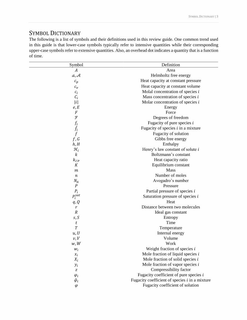
SYMBOL DICTIONARY The following is a list of symbols and their definitions used in this review guide. One common trend used

in this guide is that lower-case symbols typically refer to intensive quantities while their corresponding

upper-case symbols refer to extensive quantities. Also, an overhead dot indicates a quantity that is a function

of time.

Symbol Definition

𝐴 Area

𝒶,𝒜 Helmholtz free energy

𝑐𝑝 Heat capacity at constant pressure

𝑐𝑣 Heat capacity at constant volume

𝑐𝑖 Molal concentration of species 𝑖 𝐶𝑖 Mass concentration of species 𝑖 |𝑖| Molar concentration of species 𝑖 𝑒, 𝐸 Energy

𝐹 Force

ℱ Degrees of freedom

𝑓𝑖 Fugacity of pure species 𝑖

𝑓𝑖 Fugacity of species 𝑖 in a mixture

𝑓 Fugacity of solution

𝑓, 𝐺 Gibbs free energy

ℎ,𝐻 Enthalpy

ℋ𝑖 Henry’s law constant of solute 𝑖 𝑘 Boltzmann’s constant

𝑘𝐶𝑃 Heat capacity ratio

𝐾 Equilibrium constant

𝑚 Mass

𝑛 Number of moles

𝑁𝐴 Avogadro’s number

𝑃 Pressure

𝑃𝑖 Partial pressure of species 𝑖 𝑃𝑖

𝑠𝑎𝑡 Saturation pressure of species 𝑖

𝑞, 𝑄 Heat

𝑟 Distance between two molecules

𝑅 Ideal gas constant

𝑠, 𝑆 Entropy

𝑡 Time

𝑇 Temperature

𝑢, 𝑈 Internal energy

𝑣, 𝑉 Volume

𝑤,𝑊 Work

𝑤𝑖 Weight fraction of species 𝑖 𝑥𝑖 Mole fraction of liquid species 𝑖 𝑋𝑖 Mole fraction of solid species 𝑖 𝑦𝑖 Mole fraction of vapor species 𝑖 𝑧 Compressibility factor

𝜑𝑖 Fugacity coefficient of pure species 𝑖 �̂�𝑖 Fugacity coefficient of species 𝑖 in a mixture

𝜑 Fugacity coefficient of solution


𝛾𝑖 Activity coefficient of species 𝑖 𝜂 Efficiency factor

𝜇𝑖 Chemical potential of species 𝑖 Π Osmotic pressure

𝜌 Density

𝜈𝑖 Stoichiometric coefficient

𝜔 Pitzer acentric factor

𝜉 Extent of reaction

MEASURED THERMODYNAMIC PROPERTIES AND OTHER BASIC CONCEPTS | 5

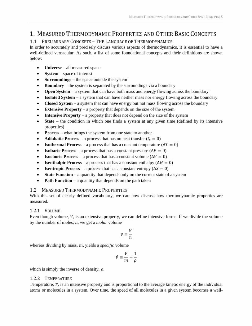
1. MEASURED THERMODYNAMIC PROPERTIES AND OTHER BASIC CONCEPTS 1.1 PRELIMINARY CONCEPTS – THE LANGUAGE OF THERMODYNAMICS In order to accurately and precisely discuss various aspects of thermodynamics, it is essential to have a

well-defined vernacular. As such, a list of some foundational concepts and their definitions are shown

below:

• Universe – all measured space

• System – space of interest

• Surroundings – the space outside the system

• Boundary – the system is separated by the surroundings via a boundary

• Open System – a system that can have both mass and energy flowing across the boundary

• Isolated System – a system that can have neither mass nor energy flowing across the boundary

• Closed System – a system that can have energy but not mass flowing across the boundary

• Extensive Property – a property that depends on the size of the system

• Intensive Property – a property that does not depend on the size of the system

• State – the condition in which one finds a system at any given time (defined by its intensive

properties)

• Process – what brings the system from one state to another

• Adiabatic Process – a process that has no heat transfer (𝑄 = 0)

• Isothermal Process – a process that has a constant temperature (Δ𝑇 = 0)

• Isobaric Process – a process that has a constant pressure (Δ𝑃 = 0)

• Isochoric Process – a process that has a constant volume (Δ𝑉 = 0)

• Isenthalpic Process – a process that has a constant enthalpy (Δ𝐻 = 0)

• Isentropic Process – a process that has a constant entropy (Δ𝑆 = 0)

• State Function – a quantity that depends only on the current state of a system

• Path Function – a quantity that depends on the path taken

1.2 MEASURED THERMODYNAMIC PROPERTIES With this set of clearly defined vocabulary, we can now discuss how thermodynamic properties are

measured.

1.2.1 VOLUME Even though volume, 𝑉, is an extensive property, we can define intensive forms. If we divide the volume

by the number of moles, 𝑛, we get a molar volume

𝑣 ≡𝑉

𝑛

whereas dividing by mass, 𝑚, yields a specific volume

𝑣 ≡𝑉

𝑚=

1

𝜌

which is simply the inverse of density, 𝜌.

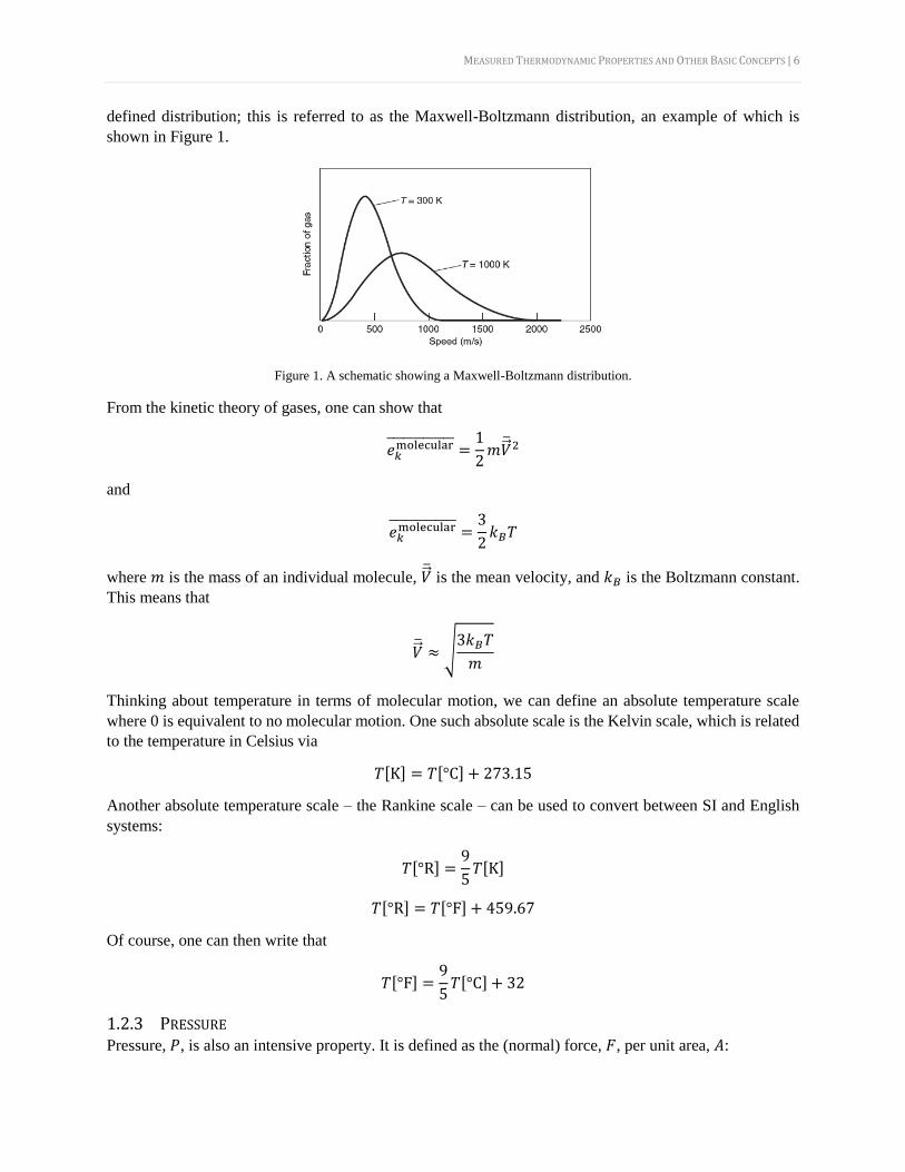
1.2.2 TEMPERATURE Temperature, 𝑇, is an intensive property and is proportional to the average kinetic energy of the individual

atoms or molecules in a system. Over time, the speed of all molecules in a given system becomes a well-


defined distribution; this is referred to as the Maxwell-Boltzmann distribution, an example of which is

shown in Figure 1.

Figure 1. A schematic showing a Maxwell-Boltzmann distribution.

From the kinetic theory of gases, one can show that

𝑒𝑘molecular̅̅ ̅̅ ̅̅ ̅̅ ̅̅ ̅̅ ̅ =

1

2𝑚�⃗� ̅2

and

𝑒𝑘molecular̅̅ ̅̅ ̅̅ ̅̅ ̅̅ ̅̅ ̅ =

3

2𝑘𝐵𝑇

where 𝑚 is the mass of an individual molecule, �⃗� ̅ is the mean velocity, and 𝑘𝐵 is the Boltzmann constant.

This means that

�⃗� ̅ ≈ √3𝑘𝐵𝑇

𝑚

Thinking about temperature in terms of molecular motion, we can define an absolute temperature scale

where 0 is equivalent to no molecular motion. One such absolute scale is the Kelvin scale, which is related

to the temperature in Celsius via

𝑇[K] = 𝑇[°C] + 273.15

Another absolute temperature scale – the Rankine scale – can be used to convert between SI and English

systems:

𝑇[°R] =9

5𝑇[K]

𝑇[°R] = 𝑇[°F] + 459.67

Of course, one can then write that

𝑇[°F] =9

5𝑇[°C] + 32

1.2.3 PRESSURE Pressure, 𝑃, is also an intensive property. It is defined as the (normal) force, 𝐹, per unit area, 𝐴:


𝑃 ≡𝐹

𝐴

Equations of state relate the measured properties 𝑇, 𝑃, and 𝑉. The ideal gas model is a simplified equation

to describe the measured properties of a perfect gas:

𝑃 =𝑛𝑅𝑇

𝑉

where 𝑅 is the ideal gas constant. The ideal gas law is based on the assumption that molecules are

infinitesimally small, round spheres that occupy negligible volume and do not experience intermolecular

attraction or repulsion.

1.3 EQUILIBRIUM

1.3.1 FUNDAMENTAL DEFINITIONS Equilibrium refers to a condition in which the state of a system neither changes with time nor has a tendency

to spontaneously change (i.e. there are no net driving forces for change). As such, equilibrium can only

occur for closed (and isolated) systems. If an open system does not change with time as it undergoes a

process, it is said to be in steady-state. With this, we will again define some important conditions:

• Mechanical equilibrium – no pressure difference between system and surroundings

• Thermal equilibrium – no temperature difference between system and surroundings

• Chemical equilibrium – no tendency for a species to change phases or chemical react

• Thermodynamic equilibrium – a system that is in mechanical, thermal, and chemical equilibrium

• Phase equilibrium – a system with more than one phase present that is in thermal and mechanical

equilibrium between the phases such that the phase has no tendency to change

• Chemical reaction equilibrium – a system undergoing chemical reactions with no more tendency

to react

• Saturation pressure – the pressure when the rate of vaporization equals the rate of condensation

(for a specific temperature), denoted 𝑃sat

• Saturation temperature – the temperature when the rate of vaporization equals the rate of

condensation (for a specific pressure), denoted 𝑇sat

• Vapor pressure – a substance’s contribution to the total pressure in a mixture at a given

temperature

• State postulate – for a system containing a pure substance, all intensive thermodynamic properties

can be determined from two independent intensive properties while all extensive thermodynamic

properties can be determined from three independent intensive properties

• Triple point – the value of 𝑃 and 𝑇 for which a pure substance has the gas, liquid, and solid phases

coexisting in thermodynamic equilibrium

• Critical temperature – the temperature at and above which vapor of a substance cannot be

liquefied

• Critical pressure – the pressure at and above which vapor of a substance cannot be liquefied

1.3.2 INDEPENDENT AND DEPENDENT THERMODYNAMIC PROPERTIES The Gibbs phase rule states that the degrees of freedom can be given by

ℑ = 𝑚 − 𝜋 + 2

THE FIRST LAW OF THERMODYNAMICS | 8

where 𝑚 is the number of chemical species in the system and 𝜋 is the number of phases. The value of ℑ is

the number of independent, intensive properties needed to constrain the properties in a given phase.

To constrain the state of a system with gas and liquid phases, the fraction that is vapor (called the quality)

can be defined:

𝑥 =𝑛𝑣

𝑛𝑙 + 𝑛𝑣

where 𝑛𝑣 and 𝑛𝑙 are the number of moles in the liquid and vapor phases, respectively. Any intensive

property can be found by proportioning its value in each phase by the fraction of the system that the phase

occupies.1

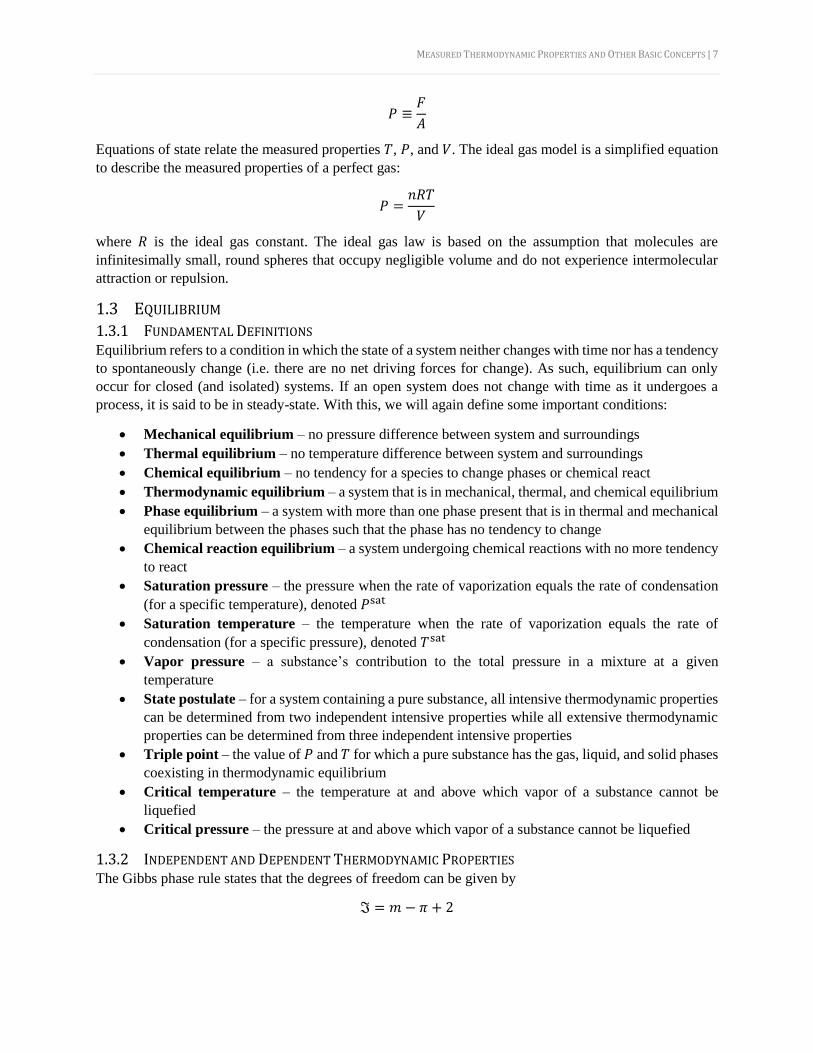
1.3.3 PHASES An example phase diagram is shown in Figure 2, denoting the effects of pressure and temperature for a

hypothetical substance.

Figure 2. A sample phase diagram. The critical temperature and critical pressure are denoted by 𝑇𝐶 and 𝑃𝐶, respectively. The triple

point is the point (𝑇𝑡𝑝, 𝑃𝑡𝑝).

2 THE FIRST LAW OF THERMODYNAMICS 2.1 DEFINITION OF THE FIRST LAW The First Law of Thermodynamics states that the total quantity of energy in the universe is constant. Phrased

another way,

Δ𝐸univ = 0

or “energy cannot be created or destroyed” although it can change forms. This can also be made to says

Δ𝐸system + Δ𝐸surroundings = 0

1 For instance, the molar volume of a liquid-vapor system can be found by 𝑣 = (1 − 𝑥)𝑣𝑙 + 𝑥𝑣𝑣.


2.2 FUNDAMENTAL DEFINITIONS • Kinetic energy –energy of motion, defined as 𝐸𝐾 =

1

2𝑚�⃗� 2

• Potential energy – energy associated with the bulk position of a system in a potential field, denoted

𝐸𝑃

• Internal energy – energy associated with the motion, position, and chemical-bonding

configuration of the individual molecules of the substances within a system, denoted 𝑈

• Sensible heat – a change in internal energy that leads to a change in temperature

• Latent heat – a change in internal energy that leads to a phase transformation

• Heat – the transfer of energy via a temperature gradient, denoted 𝑄

• Work – all forms of energy transfer other than heat, denoted 𝑊

2.3 WORK The work, 𝑊, can be described as

𝑊 = ∫𝐹 𝑑𝑥

where 𝐹 is the external force and 𝑑𝑥 is the displacement. Work can also be related to the external pressure

via

𝑊 = −∫𝑃 𝑑𝑉

which is typically referred to as 𝑃𝑉 work and can be computed by taking the area underneath a 𝑃 vs. 𝑉

curve for a process (and then negating it). In this context, a positive value of 𝑊 means that energy is

transferred from the surroundings to the system whereas a negative value means that energy is transferred

from the system to the surroundings. The same sign-convention is chosen for heat (see below).

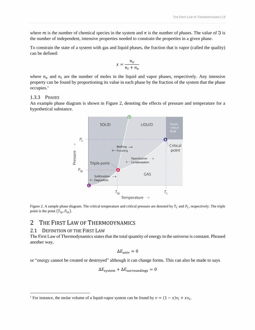
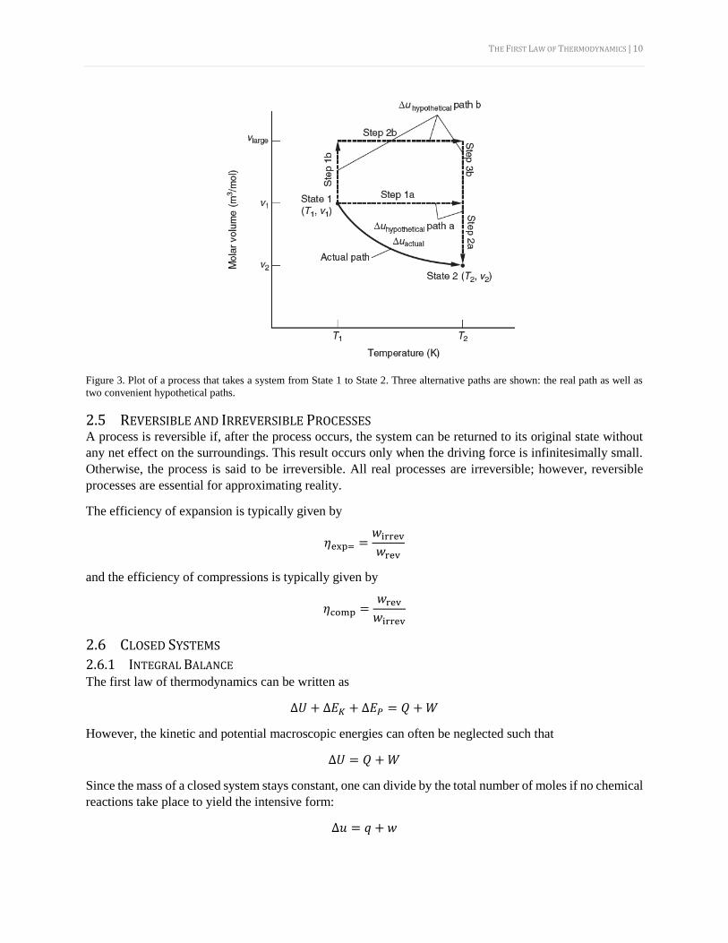
2.4 HYPOTHETICAL PATHS It is important to note that hypothetical paths can be used to find the value of a state function. Consider the

processes in Figure 3. The actual path is not easy to use for calculations, as both 𝑇 and 𝑣 are changing.

However, one can proposed alternative hypothetical paths to get from State 1 to State 2 that take advantage

of the fact that the path does not matter when computing a state function. All three paths (the real one as

well as the two hypothetical ones) will produce the same answer for Δ𝑢.


Figure 3. Plot of a process that takes a system from State 1 to State 2. Three alternative paths are shown: the real path as well as

two convenient hypothetical paths.

2.5 REVERSIBLE AND IRREVERSIBLE PROCESSES A process is reversible if, after the process occurs, the system can be returned to its original state without

any net effect on the surroundings. This result occurs only when the driving force is infinitesimally small.

Otherwise, the process is said to be irreversible. All real processes are irreversible; however, reversible

processes are essential for approximating reality.

The efficiency of expansion is typically given by

𝜂exp= =𝑤irrev

𝑤rev

and the efficiency of compressions is typically given by

𝜂comp =𝑤rev

𝑤irrev

2.6 CLOSED SYSTEMS

2.6.1 INTEGRAL BALANCE The first law of thermodynamics can be written as

Δ𝑈 + Δ𝐸𝐾 + Δ𝐸𝑃 = 𝑄 + 𝑊

However, the kinetic and potential macroscopic energies can often be neglected such that

Δ𝑈 = 𝑄 + 𝑊

Since the mass of a closed system stays constant, one can divide by the total number of moles if no chemical

reactions take place to yield the intensive form:

Δ𝑢 = 𝑞 + 𝑤


2.6.2 DIFFERENTIAL BALANCE Oftentimes in chemical engineering thermodynamics we must consider how various properties change as a

function of time. In this case, differential balances are necessary. The first law can be written similarly as

𝑑𝑈 + 𝑑𝐸𝐾 + 𝑑𝐸𝑃 = 𝛿𝑄 + 𝛿𝑊

or

𝑑𝑈 = 𝛿𝑄 + 𝛿𝑊

if we ignore kinetic and potential energy contributions.2 Of course, for a closed system we can write the

equivalent intensive form of the equation as well.

With this differential balance, we can differentiate with respect to time to yield:

𝑑𝑈

𝑑𝑡= �̇� + �̇�

2.7 ISOLATED SYSTEMS Since isolated systems do not allow for energy transfer, Δ𝑈 = 0 for this case. As such, 𝑄 + 𝑊 = 0.

2.8 OPEN SYSTEMS In open systems, mass can flow into and out of the system. This can be expressed via a mole balance as

𝑑𝑛

𝑑𝑡= ∑�̇�in

in

− ∑�̇�out

out

assuming no chemical reactions. For a stream flowing through a cross-sectional area 𝐴 with a velocity �⃗� , the molar flow rate can be written as

�̇� =𝐴�⃗�

𝑣

A system at steady-state has all differentials with respect to time being zero, so for steady-state:

∑�̇�in

in

= ∑�̇�out

out

In addition to this balance, we also must write an energy balance. The energy balance is

𝑑𝑈

𝑑𝑡+

𝑑𝐸𝐾

𝑑𝑡+

𝑑𝐸𝑃

𝑑𝑡

= ∑�̇�in

in

(𝑢 + 𝑒𝐾 + 𝑒𝑃)in − ∑�̇�out

out

(𝑢 + 𝑒𝐾 + 𝑒𝑃)out + �̇�

+ [�̇�𝑠 + ∑�̇�in

in

(𝑃𝑣)in + ∑�̇�out

out

(−𝑃𝑣)out]

In steady-state, this reads

2 The 𝑑 differential operator is used for state functions whereas the 𝛿 differential operator is used for path functions.


0 = ∑�̇�in

in


out

(𝑢 + 𝑒𝐾 + 𝑒𝑃)out + �̇�

+ [�̇�𝑠 + ∑�̇�in

in


out

(−𝑃𝑣)out]

The left two terms refer to the energy flowing into and out of the system whereas the last two terms refer

to the flow work from the inlet and outlet streams. The �̇�𝑠 term refers to the shaft work, or the useful work

that is obtained from the system.

The above expression can be algebraically rearranged to read

0 = ∑�̇�in

in

[(𝑢 + 𝑃𝑣) + 𝑒𝐾 + 𝑒𝑃]in − ∑�̇�out

out

[(𝑢 + 𝑃𝑣) + 𝑒𝐾 + 𝑒𝑃]out + �̇� + �̇�𝑠

This form is especially enlightening, as there is a frequent 𝑢 + 𝑃𝑣 term. This is enthalpy:

𝐻 ≡ 𝑈 + 𝑃𝑉

or

ℎ ≡ 𝑢 + 𝑃𝑣

This then means the energy balance can be written as

0 = ∑�̇�in

in

[ℎ + 𝑒𝐾 + 𝑒𝑃]in − ∑�̇�out

out

[ℎ + 𝑒𝐾 + 𝑒𝑃]out + �̇� + �̇�𝑠

Neglecting kinetic and potential energy contributions yields

0 = ∑�̇�in

in

ℎin − ∑�̇�out

out

ℎout + �̇� + �̇�𝑠

2.9 OPEN-SYSTEM ENERGY BALANCE ON PROCESS EQUIPMENT

2.9.1 INTRODUCTION For these problems, it is best to start with a general energy balance, such as the one shown in the previous

section:

𝑑𝑈

𝑑𝑡+

𝑑𝐸𝐾

𝑑𝑡+

𝑑𝐸𝑃

𝑑𝑡

= ∑�̇�in

in


out

(𝑢 + 𝑒𝐾 + 𝑒𝑃)out + �̇�

+ [�̇�𝑠 + ∑�̇�in

in


out

(−𝑃𝑣)out]

From here, approximations and assumptions can be made to simplify the problem further. Generally

speaking, it is best to write out the general mass and energy balances at the start of any chemical engineering

problem. The mass balances for open-system process equipment is typically just

�̇�in = �̇�out


2.9.2 NOZZLES AND DIFFUSERS These devices convert between internal energy and kinetic energy by changing the cross-sectional area

through which a fluid flows to change the bulk flow velocity. A nozzle constricts the cross-sectional area

to increase the flow whereas a diffuser increases the cross-sectional area to decrease the flow. Note that the

cross-sectional area and velocity can be related by

𝐴in�⃗� in = 𝐴out�⃗� out

Assuming steady-state (i.e. Δ�̇� = 0 if no chemical reactions are occurring, all time-derivative terms are

zero), no shaft-work (i.e. �̇�𝑠 = 0), no heat flow (i.e. �̇� = 0), the general energy balance becomes

(ℎ + 𝑒𝐾)in = (ℎ + 𝑒𝐾)out

2.9.3 TURBINES AND PUMPS These processes involve the transfer of energy via shaft work. Turbines put out useful work whereas pumps

put useful work into the system. Assuming steady-state and that the heat flow is zero (i.e. �̇� = 0) then

�̇�𝑠

�̇�= Δ(ℎ + 𝑒𝐾 + 𝑒𝑃)

2.9.4 HEAT EXCHANGERS Heat exchangers heat up or cool down a fluid through thermal contact with another fluid at a different

temperature, so it is converting between enthalpy and heat. Assuming steady-state, no shaft-work (i.e. �̇�𝑠 =

0), and no change in kinetic or potential energies (i.e. Δ𝑒𝐾 = Δ𝑒𝑃 = 0) then

�̇�

�̇�= Δℎ

2.9.5 THROTTLING DEVICES Throttling devices reduce the pressure of flowing streams, typically via a partially opened valve or porous

plug. This is most often done to liquefy a gas. These devices have negligible heat loss (i.e. �̇� = 0) due to

the small amount of time the fluid is in the device. Assuming steady-state and no shaft-work then

Δℎ = 0

2.10 THERMODYNAMIC DATA FOR 𝑈 AND 𝐻

2.10.1 HEAT CAPACITY The heat capacity at constant volume, 𝑐𝑣, can be defined as

𝑐𝑣 ≡ (𝜕𝑢

𝜕𝑇)𝑣

From this, it is clear that

Δ𝑢 = ∫𝑐𝑣 𝑑𝑇

The heat capacity at constant pressure, 𝑐𝑃, can be defined as

𝑐𝑃 ≡ (𝜕ℎ

𝜕𝑇)𝑃


From this, it is clear that

Δℎ = ∫𝑐𝑝 𝑑𝑇

For liquids and solids,

𝑐𝑃 ≈ 𝑐𝑣 [liquids and solids]

For ideal gases,

𝑐𝑃 − 𝑐𝑣 = 𝑅 [ideal gas]

2.10.2 LATENT HEAT When a substance changes phases, there is a substantial change in internal energy due to the latent heat of

transformation. These are typically reported as enthalpies (e.g. enthalpy of vaporization) at 1 bar, which is

the normal boiling point, 𝑇𝑏. Therefore, the enthalpy of heating water originally at 𝑇1 to steam at a

temperature 𝑇2 where 𝑇1 < 𝑇𝑏 < 𝑇2, for example, would be

Δℎ = ∫ 𝑐𝑝𝑙

𝑇𝑏

𝑇1

𝑑𝑇 + Δℎvap,𝑇𝑏+ ∫ 𝑐𝑃

𝑣

𝑇2

𝑇𝑏

𝑑𝑇

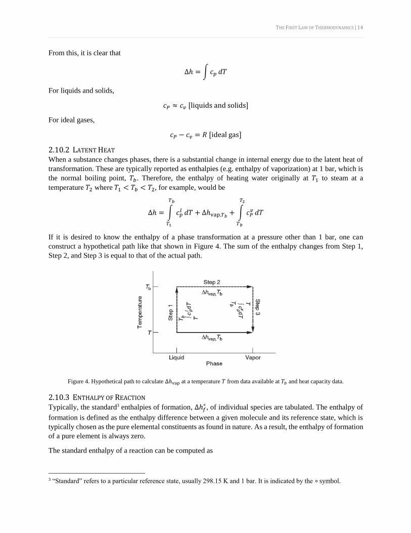
If it is desired to know the enthalpy of a phase transformation at a pressure other than 1 bar, one can

construct a hypothetical path like that shown in Figure 4. The sum of the enthalpy changes from Step 1,

Step 2, and Step 3 is equal to that of the actual path.

Figure 4. Hypothetical path to calculate Δℎvap at a temperature 𝑇 from data available at 𝑇𝑏 and heat capacity data.

2.10.3 ENTHALPY OF REACTION Typically, the standard3 enthalpies of formation, Δℎ𝑓

∘ , of individual species are tabulated. The enthalpy of

formation is defined as the enthalpy difference between a given molecule and its reference state, which is

typically chosen as the pure elemental constituents as found in nature. As a result, the enthalpy of formation

of a pure element is always zero.

The standard enthalpy of a reaction can be computed as

3 “Standard” refers to a particular reference state, usually 298.15 K and 1 bar. It is indicated by the ∘ symbol.


Δℎrxn∘ = ∑𝜈𝑖Δℎ𝑓

∘

Here, 𝜈𝑖 is the stoichiometric coefficient. For a balanced reaction 𝑎A → bB, the stoichiometric coefficient

of 𝐴 would be 𝜈𝐴 = −𝑎 and the stoichiometric coefficient of 𝐵 would be 𝜈𝐵 = 𝑏. A reaction that releases

heat is called exothermic and has a negative enthalpy of reaction, whereas a reaction that absorbs heat is

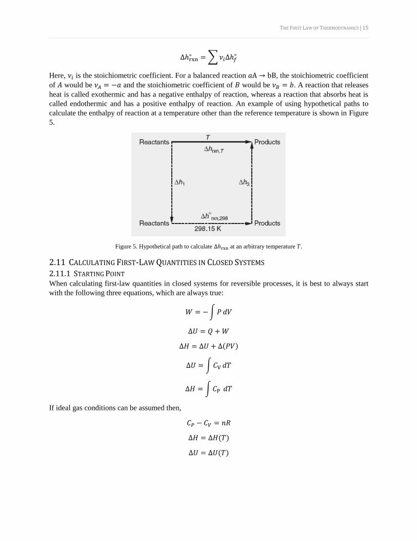
called endothermic and has a positive enthalpy of reaction. An example of using hypothetical paths to

calculate the enthalpy of reaction at a temperature other than the reference temperature is shown in Figure

5.

Figure 5. Hypothetical path to calculate Δℎrxn at an arbitrary temperature 𝑇.

2.11 CALCULATING FIRST-LAW QUANTITIES IN CLOSED SYSTEMS

2.11.1 STARTING POINT When calculating first-law quantities in closed systems for reversible processes, it is best to always start

with the following three equations, which are always true:

𝑊 = −∫𝑃 𝑑𝑉

Δ𝑈 = 𝑄 + 𝑊

Δ𝐻 = Δ𝑈 + Δ(𝑃𝑉)

Δ𝑈 = ∫𝐶V 𝑑𝑇

Δ𝐻 = ∫𝐶P 𝑑𝑇

If ideal gas conditions can be assumed then,

𝐶𝑃 − 𝐶𝑉 = 𝑛𝑅

Δ𝐻 = Δ𝐻(𝑇)

Δ𝑈 = Δ𝑈(𝑇)


2.11.2 REVERSIBLE, ISOBARIC PROCESS Since pressure is constant:4

𝑊 = −𝑃Δ𝑉

We then have the following relationships for enthalpy:

𝑄𝑃 = Δ𝐻

Δ𝐻 = ∫𝐶𝑃 𝑑𝑇

Δ𝐻 = Δ𝑈 + 𝑃Δ𝑉

2.11.3 REVERSIBLE, ISOCHORIC PROCESS Since volume is constant:

𝑊 = 0

We then have the following relationships for the internal energy:

𝑄𝑉 = Δ𝑈

Δ𝑈 = ∫𝐶𝑉 𝑑𝑇

Δ𝐻 = Δ𝑈 + 𝑉Δ𝑃

2.11.4 REVERSIBLE, ISOTHERMAL PROCESS If one is dealing with an ideal gas, Δ𝑈 and Δ𝐻 are only functions of temperature, so

Δ𝑈 = Δ𝐻 = 0

Due to the fact that Δ𝑈 = 𝑄 + 𝑊,

𝑄 = −𝑊

For an ideal gas, integrate the ideal gas law with respect to 𝑉 to get

𝑊 = −𝑛𝑅𝑇 ln (𝑉2

𝑉1) = 𝑛𝑅𝑇 ln (

𝑃2

𝑃1)

2.11.5 REVERSIBLE, ADIABATIC PROCESS By definition the heat exchange is zero, so:

𝑄 = 0

Due to the fact that Δ𝑈 = 𝑄 + 𝑊,

𝑊 = Δ𝑈

4 When dealing with thermodynamic quantities, it is important to keep track of units. For instance, computing 𝑊 =−𝑃Δ𝑉 will get units of [Pressure][Volume]. To convert this to a unit of [Energy], one must use a conversion factor,

such as (8.3145 J/mol K)/(0.08206 L atm/mol K) = 101.32 J/L*atm.


The following relationships can also be derived for a system with constant heat capacity:

𝑇2

𝑇1= (

𝑉1

𝑉2)

𝑅𝐶𝑉

(𝑃1

𝑃2)𝑅

= (𝑇1

𝑇2)𝐶𝑃

𝑃1𝑉1𝐶𝑃/𝐶𝑉 = 𝑃2𝑉2

𝐶𝑃/𝐶𝑉

This means that5

𝑊 = Δ𝑈 =Δ(𝑃𝑉)

𝐶𝑃/𝐶𝑉 − 1=

𝑛𝑅Δ𝑇

𝐶𝑃/𝐶𝑉 − 1

2.11.6 IRREVERSIBLE, ADIABATIC EXPANSION INTO A VACUUM For this case,

𝑄 = 𝑊 = Δ𝑈 = Δ𝐻 = 0

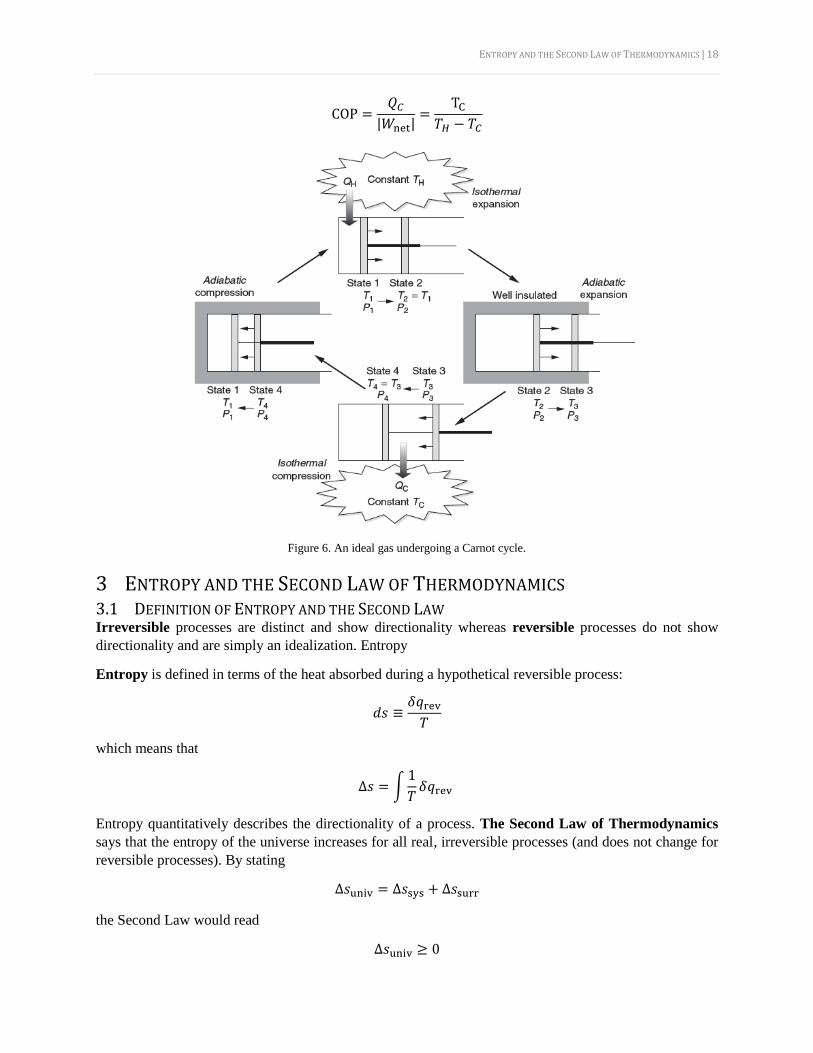
2.12 THERMODYNAMIC CYCLES AND THE CARNOT CYCLE A thermodynamic cycle always returns to the same state it was in initially, meaning all state functions are

zero for the net cycle. For a Carnot cycle, there are four stages, as outlined in Figure 6. Since all state

functions are zero for the net cycle, we know that

Δ𝑈cycle = Δ𝐻cycle = 0

Due to the First Law of Thermodynamics,

−𝑊net = 𝑄net

The net work and the neat heat can be computed by summing up the individual work and heat from each of

the four processes. For a Carnot cycle, there is a negative net work.

The following relationships apply to the Carnot cycle:

𝑃2

𝑃1=

𝑃3

𝑃4

and

𝑄𝐻

𝑄𝐶= −

𝑇𝐻

𝑇𝐶

The efficiency of the Carnot cycle is defined as

𝜂 ≡net work

wasted heat=

|𝑊net|

𝑄𝐻= 1 −

𝑇𝐶

𝑇𝐻

The efficiency of the Carnot cycle run in reverse (i.e. a Carnot refrigerator) is characterized by the

coefficient of performance, given by

5 The term Δ(𝑃𝑉) ≡ 𝑃2𝑉2 − 𝑃1𝑉1.

ENTROPY AND THE SECOND LAW OF THERMODYNAMICS | 18

COP =𝑄𝐶

|𝑊net|=

TC

𝑇𝐻 − 𝑇𝐶

Figure 6. An ideal gas undergoing a Carnot cycle.

3 ENTROPY AND THE SECOND LAW OF THERMODYNAMICS 3.1 DEFINITION OF ENTROPY AND THE SECOND LAW Irreversible processes are distinct and show directionality whereas reversible processes do not show

directionality and are simply an idealization. Entropy

Entropy is defined in terms of the heat absorbed during a hypothetical reversible process:

𝑑𝑠 ≡𝛿𝑞rev

𝑇

which means that

Δ𝑠 = ∫1

𝑇𝛿𝑞rev

Entropy quantitatively describes the directionality of a process. The Second Law of Thermodynamics

says that the entropy of the universe increases for all real, irreversible processes (and does not change for

reversible processes). By stating

Δ𝑠univ = Δ𝑠sys + Δ𝑠surr

the Second Law would read

Δ𝑠univ ≥ 0


3.2 THE SECOND LAW OF THERMODYNAMICS FOR CLOSED SYSTEMS

3.2.1 REVERSIBLE, ADIABATIC PROCESSES Since the process is reversible and there is no heat transfer6,

Δ𝑠 = 0, Δ𝑠surr = 0, Δ𝑠univ = 0

3.2.2 REVERSIBLE, ISOTHERMAL PROCESSES Since temperature is constant,

Δ𝑠 =𝑞rev

𝑇

If the ideal gas assumption can be made, then Δ𝑢 = 0 such that 𝑞rev = 𝑤rev = −∫𝑃 𝑑𝑉. Plug in the ideal

gas law to get

Δ𝑠 = −𝑅 ln (𝑃2

𝑃1)

Since all reversible processes have no change in the entropy of the universe (i.e. Δ𝑠univ = 0), we can say

that Δ𝑠surr = −Δ𝑠.

3.2.3 REVERSIBLE, ISOBARIC PROCESSES Since 𝛿𝑞𝑃 = 𝑑ℎ = 𝑐𝑃 𝑑𝑇 for isobaric processes,

Δ𝑠 = ∫𝑐𝑃

𝑇𝑑𝑇



3.2.4 REVERSIBLE, ISOCHORIC PROCESSES Since 𝛿𝑞𝑉 = 𝑑𝑢 = 𝑐𝑉 𝑑𝑇 for isochoric processes,

Δ𝑠 = ∫𝑐𝑉

𝑇𝑑𝑇



3.2.5 REVERSIBLE PHASE CHANGE AT CONSTANT 𝑇 AND 𝑃 In this case, 𝑞rev is the latent heat of the phase transition. As such,

Δ𝑠 =𝑞𝑃

𝑇=

Δℎtransition

𝑇



6 It will be tacitly assumed any quantity without a subscript refers to that the system.


3.2.6 IRREVERSIBLE PROCESSES FOR IDEAL GASES A general expression can be written to describe the entropy change of an ideal gas. Two equivalent

expressions are:

Δ𝑠 = ∫𝑐𝑉

𝑇𝑑𝑇 + 𝑅 ln (

𝑉2

𝑉1)

and


𝑇𝑑𝑇 − 𝑅 ln (

𝑃2

𝑃1)

In order to find the entropy change of the universe, one must think about the conditions of the problem

statement. If the real process is adiabatic, then 𝑞surr = 0 and then Δ𝑠surr = 0 such that Δ𝑠univ = Δ𝑠. If the

real process is isothermal, note that 𝑞 = 𝑤 from the First Law of Thermodynamics (i.e. Δ𝑢 = 0) amd that

due to conservation of energy 𝑞surr = −𝑞. Once 𝑞surr is known, simply use Δ𝑠surr =𝑞surr

𝑇. The entropy

change in the universe is then Δ𝑠univ = Δ𝑠 + Δ𝑠surr.

If the ideal gas approximation cannot be made, try splitting up the irreversible process into hypothetical,

reversible pathways that may be easier to calculate.

3.2.7 ENTROPY CHANGE OF MIXING If we assume that we are mixing different inert, ideal gases then the entropy of mixing is

Δ𝑆mix = 𝑅 ∑𝑛𝑖 ln (𝑉𝑓

𝑉𝑖)

For an ideal gas at constant 𝑇 and 𝑃 then

Δ𝑆mix = −𝑅 ∑𝑛𝑖 ln (𝑃𝑖

𝑃tot) = −𝑅 ∑𝑛𝑖 ln(𝑦𝑖)

where 𝑃𝑖 is the partial pressure of species 𝑖 and 𝑦𝑖 is the mole fraction of species 𝑖.

3.3 THE SECOND LAW OF THERMODYNAMICS FOR OPEN SYSTEMS Since mass can flow into and out of an open system, the Second Law must be written with respect to time:

(𝑑𝑆

𝑑𝑡)univ

= (𝑑𝑆

𝑑𝑡)sys

+ (𝑑𝑆

𝑑𝑡)surr

≥ 0

At steady-state,

(𝑑𝑆

𝑑𝑡)sys

= 0

If there is a constant surrounding temperature, then

(𝑑𝑆

𝑑𝑡)surr

= ∑�̇�out𝑠out − ∑�̇�in𝑠in −�̇�

𝑇surr


3.4 THE MECHANICAL ENERGY BALANCE For steady-state, reversible processes with one stream in and one stream out, the mechanical energy balance

is

𝑊𝑠̇

�̇�= ∫𝑣 𝑑𝑃 + Δ𝑒𝐾 + Δ𝑒𝑃

which can frequently be written as

�̇�𝑠

�̇�= ∫𝑣 𝑑𝑃 + MW[

Δ(�⃗� 2)

2] + MW𝑔Δ𝑧

Where MW refers to the molecular weight of the fluid. The latter equation is referred to as the Bernoulli

Equation.

3.5 VAPOR-COMPRESSION POWER AND REFRIGERATION CYCLES

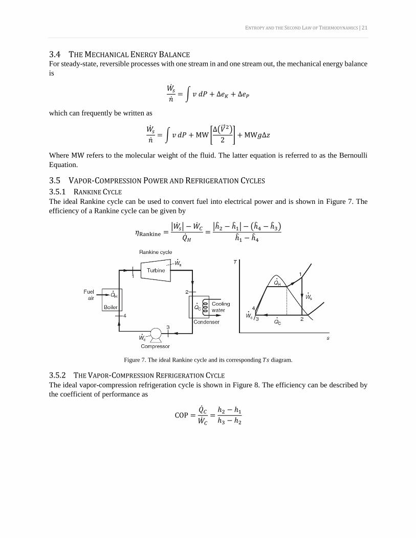
3.5.1 RANKINE CYCLE The ideal Rankine cycle can be used to convert fuel into electrical power and is shown in Figure 7. The

efficiency of a Rankine cycle can be given by

𝜂Rankine =|�̇�𝑠| − �̇�𝐶

�̇�𝐻

=|ℎ̂2 − ℎ̂1| − (ℎ̂4 − ℎ̂3)

ℎ̂1 − ℎ̂4

Figure 7. The ideal Rankine cycle and its corresponding 𝑇𝑠 diagram.

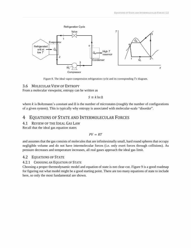
3.5.2 THE VAPOR-COMPRESSION REFRIGERATION CYCLE The ideal vapor-compression refrigeration cycle is shown in Figure 8. The efficiency can be described by

the coefficient of performance as

COP =�̇�𝐶

�̇�𝐶

=ℎ2 − ℎ1

ℎ3 − ℎ2

EQUATIONS OF STATE AND INTERMOLECULAR FORCES | 22

Figure 8. The ideal vapor-compression refrigeration cycle and its corresponding 𝑇𝑠 diagram.

3.6 MOLECULAR VIEW OF ENTROPY From a molecular viewpoint, entropy can be written as

𝑆 ≡ 𝑘 lnΩ

where 𝑘 is Boltzmann’s constant and Ω is the number of microstates (roughly the number of configurations

of a given system). This is typically why entropy is associated with molecular-scale “disorder”.

4 EQUATIONS OF STATE AND INTERMOLECULAR FORCES 4.1 REVIEW OF THE IDEAL GAS LAW Recall that the ideal gas equation states

𝑃𝑉 = 𝑅𝑇

and assumes that the gas consists of molecules that are infinitesimally small, hard round spheres that occupy

negligible volume and do not have intermolecular forces (i.e. only exert forces through collisions). As

pressure decreases and temperature increases, all real gases approach the ideal gas limit.

4.2 EQUATIONS OF STATE

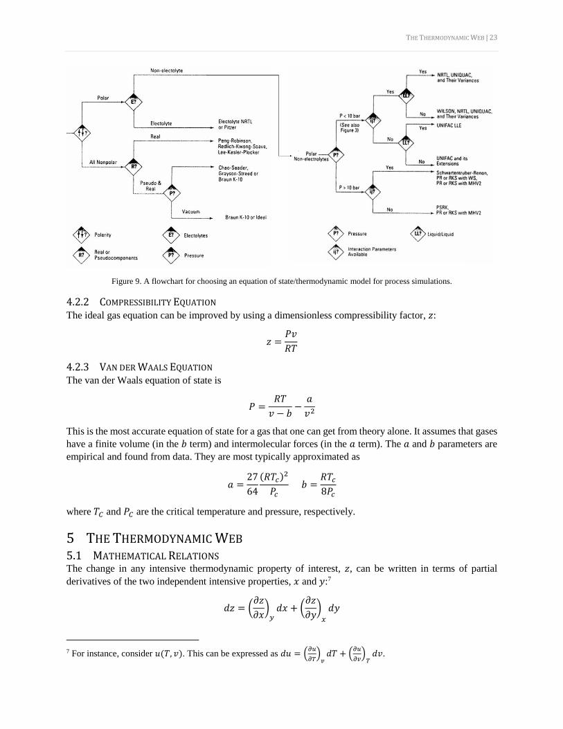
4.2.1 CHOOSING AN EQUATION OF STATE Choosing a proper thermodynamic model and equation of state is not clear-cut. Figure 9 is a good roadmap

for figuring out what model might be a good starting point. There are too many equations of state to include

here, so only the most fundamental are shown.

THE THERMODYNAMIC WEB | 23

Figure 9. A flowchart for choosing an equation of state/thermodynamic model for process simulations.

4.2.2 COMPRESSIBILITY EQUATION The ideal gas equation can be improved by using a dimensionless compressibility factor, 𝑧:

𝑧 =𝑃𝑣

𝑅𝑇

4.2.3 VAN DER WAALS EQUATION The van der Waals equation of state is

𝑃 =𝑅𝑇

𝑣 − 𝑏−

𝑎

𝑣2

This is the most accurate equation of state for a gas that one can get from theory alone. It assumes that gases

have a finite volume (in the 𝑏 term) and intermolecular forces (in the 𝑎 term). The 𝑎 and 𝑏 parameters are

empirical and found from data. They are most typically approximated as

𝑎 =27

64

(𝑅𝑇𝑐)2

𝑃𝑐 𝑏 =

𝑅𝑇𝑐

8𝑃𝑐

where 𝑇𝐶 and 𝑃𝐶 are the critical temperature and pressure, respectively.

5 THE THERMODYNAMIC WEB 5.1 MATHEMATICAL RELATIONS The change in any intensive thermodynamic property of interest, 𝑧, can be written in terms of partial

derivatives of the two independent intensive properties, 𝑥 and 𝑦:7

𝑑𝑧 = (𝜕𝑧

𝜕𝑥)𝑦𝑑𝑥 + (

𝜕𝑧

𝜕𝑦)𝑥

𝑑𝑦

7 For instance, consider 𝑢(𝑇, 𝑣). This can be expressed as 𝑑𝑢 = (

𝜕𝑢

𝜕𝑇)𝑣𝑑𝑇 + (

𝜕𝑢

𝜕𝑣)

𝑇𝑑𝑣.


The following relationship is also true:

(𝜕𝑥

𝜕𝑧)𝑦(𝜕𝑦

𝜕𝑥)𝑧(𝜕𝑧

𝜕𝑦)𝑥

= −1

5.2 DERIVED THERMODYNAMIC QUANTITIES The measured properties of a system are 𝑃, 𝑣, 𝑇 and composition. The fundamental thermodynamic

properties are 𝑢 and 𝑠, as previously discussed. There are also derived thermodynamic properties. One of

which is ℎ. There are also two other convenient derived properties: 𝑎, which is Helmholtz free energy, and

𝑔, which is Gibbs free energy. The derived thermodynamic properties have the following relationships:

ℎ ≡ 𝑢 + 𝑃𝑣 𝑎 ≡ 𝑢 − 𝑇𝑠 𝑔 ≡ ℎ − 𝑇𝑠

Also recall the heat capacity definitions discussed earlier:

𝑐𝑣 = (𝜕𝑢

𝜕𝑇)𝑣 𝑐𝑝 = (

𝜕ℎ

𝜕𝑇)𝑃

5.3 FUNDAMENTAL PROPERTY RELATIONS The First Law of Thermodynamics states

𝑑𝑢 = 𝛿𝑞rev + 𝛿𝑤rev

Now consider enthalpy:

𝑑ℎ = 𝑑𝑢 + 𝑑(𝑃𝑣)

Similarly, consider Helmholtz free energy:

𝑑𝑎 = 𝑑𝑢 − 𝑑(𝑇𝑠)

Finally, consider Gibbs free energy:

𝑑𝑔 = 𝑑ℎ − 𝑑(𝑇𝑠)

Recall that 𝛿𝑞rev = 𝑇 𝑑𝑠 from the Second Law and 𝛿𝑤rev = −𝑃𝑑𝑣. With this, we can write a new

expression for 𝑑𝑢 and therefore new expressions for 𝑑ℎ, 𝑑𝑎, and 𝑑𝑔 as well. These are called the

fundamental property relations:

𝑑𝑢 = 𝑇 𝑑𝑠 − 𝑃 𝑑𝑣

𝑑ℎ = 𝑇 𝑑𝑠 + 𝑣 𝑑𝑃

𝑑𝑎 = −𝑃 𝑑𝑣 − 𝑠 𝑑𝑇

𝑑𝑔 = 𝑣 𝑑𝑃 − 𝑠 𝑑𝑇

With these expressions, one can write a number of unique relationships by holding certain values constant.

By doings so, one yields:

(𝜕𝑢

𝜕𝑠)𝑣

= 𝑇 (𝜕𝑢

𝜕𝑣)𝑠= −𝑃

(𝜕ℎ

𝜕𝑠)𝑃

= 𝑇 (𝜕ℎ

𝜕𝑃)𝑠= 𝑣


(𝜕𝑎

𝜕𝑇)𝑣

= −𝑠 (𝜕𝑎

𝜕𝑣)𝑇

= −𝑃

(𝜕𝑔

𝜕𝑇)𝑃

= −𝑠 (𝜕𝑔

𝜕𝑃)𝑇

= 𝑣

5.4 MAXWELL RELATIONS The Maxwell Relations can be derived by applying Euler’s Reciprocity to the derivative of the equation of

state. The Euler Reciprocity is

𝜕2𝑧

𝜕𝑥 𝜕𝑦=

𝜕2𝑧

𝜕𝑦 𝜕𝑥

Another useful identity to keep in mind is

𝜕2𝑧

𝜕𝑥 𝜕𝑦= (

𝜕

𝜕𝑥(𝜕𝑧

𝜕𝑦)𝑥

)𝑦

These mathematical relationships allow one to derive what are called the Maxwell Relations.8 These are

shown below:

𝜕2𝑢

𝜕𝑠 𝜕𝑣: (

𝜕𝑇

𝜕𝑣)𝑠= −(

𝜕𝑃

𝜕𝑠)𝑣

𝜕2ℎ

𝜕𝑠 𝜕𝑃: (

𝜕𝑇

𝜕𝑃)𝑠= (

𝜕𝑣

𝜕𝑠)𝑃

𝜕2𝑎

𝜕𝑇𝜕𝑣: (

𝜕𝑠

𝜕𝑣)𝑇

= (𝜕𝑃

𝜕𝑇)𝑣

𝜕2𝑔

𝜕𝑇 𝜕𝑃: (

𝜕𝑠

𝜕𝑃)𝑇

= −(𝜕𝑣

𝜕𝑇)𝑃

By using the thermodynamic property relations in conjunction with the Maxwell Relations, one can also

write heat capacities in terms of 𝑇 and 𝑠:

𝑐𝑣 = 𝑇 (𝜕𝑠

𝜕𝑇)𝑣 𝑐𝑝 = 𝑇 (

𝜕𝑠

𝜕𝑇)𝑃

5.5 DEPENDENT OF STATE FUNCTIONS ON 𝑇, 𝑃, AND 𝑣 With the previous information, one can find the dependence of any state function on 𝑇, 𝑃, or 𝑣 quite easily.

The procedure to do so can be broken down as follows:9

1) Start with the fundamental property relation for 𝑑𝑢, 𝑑ℎ, 𝑑𝑎, or 𝑑𝑔

2) Impose the conditions of constant 𝑇, 𝑃, or 𝑣

3) Divide by 𝑑𝑃𝑇 , 𝑑𝑣𝑇 , 𝑑𝑇𝑣, or 𝑑𝑇𝑃 as necessary

8 For instance, consider

𝜕2𝐺

𝜕𝑇 𝜕𝑃. This can be rewritten as

𝜕2𝐺

𝜕𝑇 𝜕𝑃= (

𝜕

𝜕𝑇(𝜕𝐺

𝜕𝑃)

𝑇)𝑃 using Euler’s Reciprocity. Using the

appropriate fundamental property relation, 𝜕2𝐺

𝜕𝑇 𝜕𝑃= (

𝜕

𝜕𝑇(𝜕𝐺

𝜕𝑃)

𝑇)𝑃

= (𝜕𝑉

𝜕𝑇)𝑃

.

9 For instance, consider trying to find what (𝜕𝑢

𝜕𝑣)

𝑇 can also be written as. Write out the fundamental property relation:

𝑑𝑢 = 𝑇 𝑑𝑠 − 𝑃 𝑑𝑣. Then impose constant 𝑇 and divide by 𝑑𝑣𝑇: (𝜕𝑢

𝜕𝑣)

𝑇= 𝑇 (

𝜕𝑠

𝜕𝑣)

𝑇− 𝑃. Recognize that (

𝜕𝑠

𝜕𝑣)

𝑇=

𝛽𝑇

𝜅

from the Maxwell Relations such that (𝜕𝑢

𝜕𝑣)

𝑇=

𝛽𝑇

𝜅− 𝑃.


4) Use a Maxwell relation or other identity to eliminate any terms with entropy change in the

numerator (if desired)

It is useful to know the following identities:

𝛽 ≡1

𝑣(𝜕𝑣

𝜕𝑇)𝑃 𝜅 ≡ −

1

𝑣(𝜕𝑣

𝜕𝑃)𝑇

where 𝛽 and 𝜅 are the thermal expansion coefficient and isothermal compressibility, respectively.

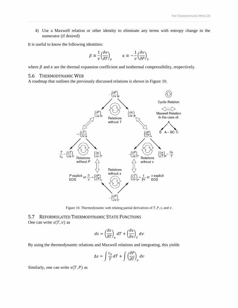
5.6 THERMODYNAMIC WEB A roadmap that outlines the previously discussed relations is shown in Figure 10.

Figure 10. Thermodynamic web relating partial derivatives of 𝑇, 𝑃, 𝑠, and 𝑣.

5.7 REFORMULATED THERMODYNAMIC STATE FUNCTIONS One can write 𝑠(𝑇, 𝑣) as

𝑑𝑠 = (𝜕𝑠


𝜕𝑠

𝜕𝑣)𝑇𝑑𝑣

By using the thermodynamic relations and Maxwell relations and integrating, this yields

Δ𝑠 = ∫𝑐𝑣

𝑇𝑑𝑇 + ∫(

𝜕𝑃

𝜕𝑇)𝑣𝑑𝑣

Similarly, one can write 𝑠(𝑇, 𝑃) as


𝑑𝑠 = (𝜕𝑠

𝜕𝑇)𝑃𝑑𝑇 + (

𝜕𝑠

𝜕𝑃)𝑇𝑑𝑃

By using the thermodynamic relations and Maxwell relations and integrating, this yields


𝑇𝑑𝑇 − (

𝜕𝑣

𝜕𝑇)𝑃𝑑𝑃

One can do the same with 𝑢. If one writes 𝑢(𝑇, 𝑣) then

𝑑𝑢 = (𝜕𝑢


𝜕𝑢

𝜕𝑣)𝑇𝑑𝑣

After much substitution one can come to find that

Δ𝑢 = ∫𝑐𝑣𝑑𝑇 + ∫[𝑇 (𝜕𝑃

𝜕𝑇)𝑣− 𝑃]𝑑𝑣

If one write ℎ(𝑇, 𝑃) as

𝑑ℎ = (𝜕ℎ

𝜕𝑇)𝑃𝑑𝑇 + (

𝜕ℎ

𝜕𝑃)𝑇𝑑𝑃

then after much substitution

Δℎ = ∫𝑐𝑃𝑑𝑇 + ∫[−𝑇 (𝜕𝑣

𝜕𝑇)𝑃

+ 𝑣] 𝑑𝑃

Documents

Chemical Engineering Thermodynamics - Tufts UniversityMEASURED THERMODYNAMIC PROPERTIES AND OTHER BASIC CONCEPTS | 5 1. MEASURED THERMODYNAMIC PROPERTIES AND OTHER BASIC CONCEPTS 1.1