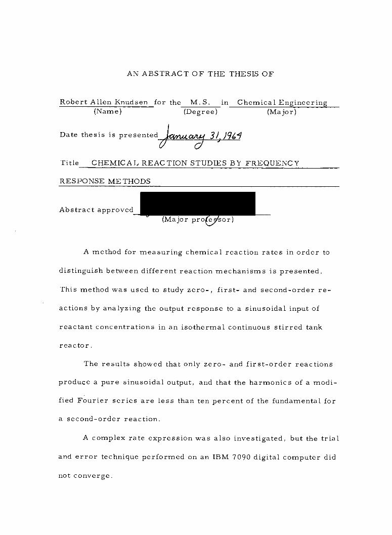
AN ABSTRACT OF THE THESIS OF

Robert Allen Knudsen for the M.S. in Chemical Engineering (Name) (Degree) (Major)

Date thesis is presented

Title CHEMICAL REACTION STUDIES BY FREQUENCY

RESPONSE METHODS

Abstract approved Major pro sor

A method for measuring chemical reaction rates in order to

distinguish between different reaction mechanisms is presented.

This method was used to study zero -, first- and second -order re-

actions by analyzing the output response to a sinusoidal input of

reactant concentrations in an isothermal continuous stirred tank

reactor.

The results showed that only zero- and first -order reactions

produce a pure sinusoidal output, and that the harmonics of a modi-

fied Fourier series are less than ten percent of the fundamental for

a second -order reaction.

A complex rate expression was also investigated, but the trial

and error technique performed on an IBM 7090 digital computer did

not converge.

3,1969

If more theoretical responses are computed for other, and

more complex, rate equations, this approach can be used to distin-

guish between different reaction rate equations and consequently can

aid in determining the true reaction mechanism.

CHEMICAL REACTION STUDIES BY FREQUENCY RESPONSE METHODS

by

ROBERT ALLEN KNUDSEN

A THESIS

submitted to

OREGON STATE UNIVERSITY

in partial fulfillment of the requirements for the

degree of

MASTER OF SCIENCE

June 1964

APPROVED:

Assistant Professor Chemical Engineering

In Charge of Major

Head of Department of Chemical Engineering

Dean of Graduate School

Date thesis is presented 31, /969

ACKNOWLEDGEMENTS

The author wishes to express his appreciation to Professor

D. E. Jost for his help and encouragement during this investigation

and also his suggestions for writing the thesis. Dr. H. E. Goheen

is to be thanked for introducing me to numerical calculus, and

Dr. R. E. Gaskell deserves credit for introducing the Fourier

series solution.

The possibilities of analog computers were discovered through

limited experimental investigations performed by this author and

Professors W. W. Smith and S. A. Stone.

I am also indebted to my friend, Mr. James R. Divine, for

his help during this work.

Finally, the Engineering Experiment Station is to be thanked

for their generous financial support.

TABLE OF CONTENTS

Pag e

INTRODUCTION 1

REVIEW OF LITERATURE 3

THEORY 5

CALCULATIONAL METHODS 12

Numerical Calculus Method Analytic Steady -State Solutions Fourier Series Solution Analog Computer Solution

DISCUSSION OF RESULTS

12 12 13 15

16

Nonreacting System 16 Zero -Order Reactions 16 First -Order Reaction 17 Second -Order Reaction 19 Complex Reaction 25 Numerical Calculus Method 27 Experimental Considerations 27

CONCLUSIONS AND RECOMMENDATIONS 30

BIBLIOGRAPHY 31

NOMENCLATURE 33

APPENDICES

Appendix A Digital Computer Programs 36

Numerical Calculus Scheme 36 Fourier Series Solution of Eq. (5) for a 38

Second -Order Reaction Fourier Series Solution of Eq. (5) for a 41

Complex Rate Equation

Appendix B Analog Computer Programs

Rate Equation Not Influenced by Products Rate Equation Influenced by Products

Pag e

52

52 52

Appendix C Digital Computer Data for Second- 53 Order Reaction

LIST OF TABLES

Table Page

1 Periodic steady -state constants in the Foirier series solution for Eq. (5) when f(n) = Krk

and A = 0.5

53

2 Periodic steady -state constants in the Forier 54 series solution for Eq. (5) when f(ri) = Krk

and K = 1.0

LIST OF FIGURES

Figure Page

1 Reactor model 6

2 Amplitude ratio and phase lag for zero-order 17and nonreacting systems

3 Amplitude ratio and phase lag for first-order 18reactions

4 Mean dimensionless output concentration for 20a second-order reaction for A = 0. 5

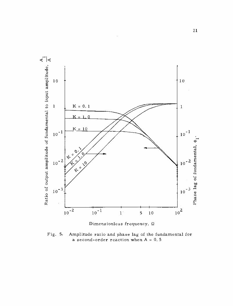
5 Amplitude ratio and phase lag of the fundamental 21for a second-order reaction when A = 0. 5

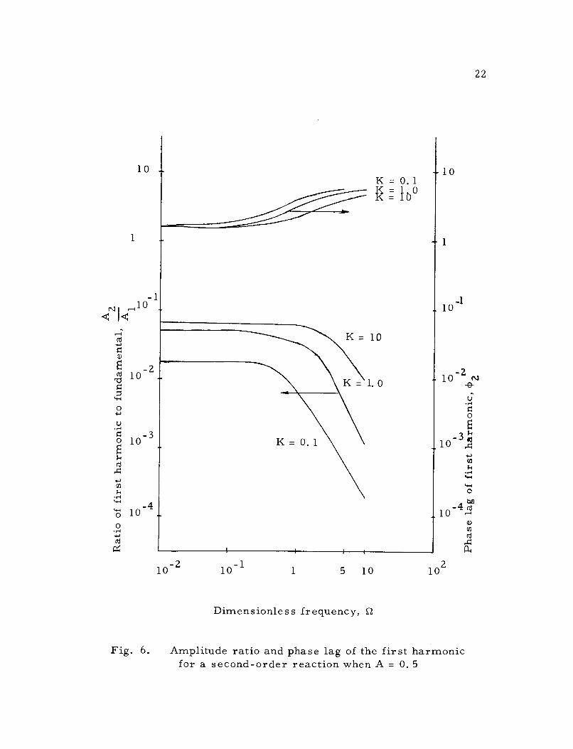
6 Amplitude ratio and phase lag of the second har- 22monic for a second-order reaction when A = 0. 5

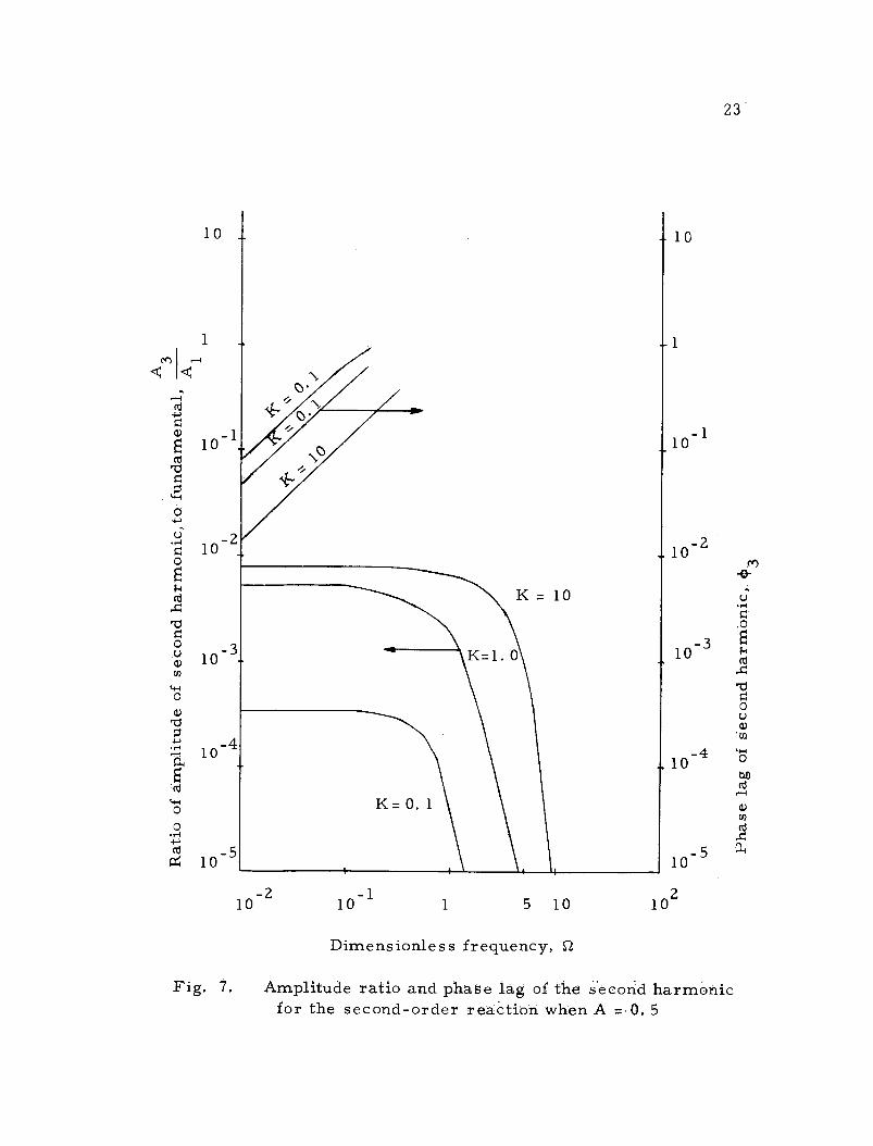
7 Amplitude ratio and phase lag of the second har- 23monic for a second-order reaction when A = 0. 5

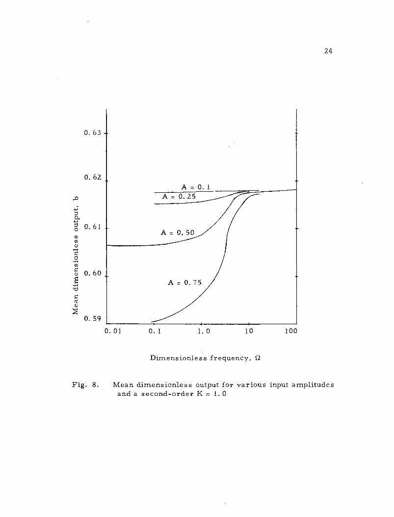
8 Mean dimensionless output for various input am- 24plitudes and a second-order reaction when K= 1. 0

9 Amplitude ratios with respect to A of fundamental 25and first harmonic to fundamental for a second-

order reaction when K = 1„0

10 Dimensionless response curves for a first- and 28second-order reactions when A=0. 1, K = 1. 0

and Q = 10

d'n11 Block diagram of analog computer for -sr =1 52

+ A sinf2G- r\ - f(n)

12 Block diagram of analog computer for—H =1 52+ A sinflG-'n - f(T),v) d0

CHEMICAL REACTION STUDIES BY FREQUENCY RESPONSE METHODS

INTRODUCTION

For a given chemical system undergoing reaction, determina-

tion of the form of the rate equation and of the constants appearing in

the equation is required for optimum design of a chemical reactor.

Knowledge of the rate equation is also a first step toward determining

the actual reaction mechanism. Once a reaction mechanism is estab-

lished, extrapolation to other concentrations and temperatures may be

achieved with a greater degree of assurance, and thus, optimum con-

ditions for conducting the reaction can be established. Therefore, a

primary aim of applied kinetic studies is to determine the rate equa-

tion, and if possible, to determine the reaction mechanism.

In general, the form of the rate equation cannot be predicted

from the stoichiometric equation, and a trial and error procedure is

required where experimental rate data are plotted to test various

postulated rate expressions. As a starting point, simple rate equa-

tions are tested; however, equations of simple form are often not

sufficient since the actual mechanism is usually complex and involves

free radicals, ions or polar substances, molecules, or other inter-

mediate species. The postulation of a particular complex reaction

mechanism from a large number of possibilities is not straight

2

forward; the choice usually being based on an intimate knowledge

of the chemistry of similar reactions, fragmentary experimental

data, and intuition.

Sometimes two or more mechanisms can be consistent with

the available rate and thermodynamic data. In these cases, speci-

fic tests, e. g. , initial rate experiments, are devised to disprove

all but one of the postulated mechanisms.

The approach presented here provides a more definitive

characterization of the chemical rate process by measuring the

frequency- response of a reacting system over a wide range of per-

turbation frequencies, input concentration amplitudes, and tempera-

ture. Theoretically, no two different rate equations will exhibit the

same response, and, therefore, this approach can distinguish be-

tween different expressions for the reaction rate and, consequently

between postulated mechanisms.

3

LITERATURE REVIEW

In the early thirties, H. S. Black (1), an electrical engineer,

used the results of H. Nyquist's (6) work on the stability of feed

back amplifiers by frequency- response analysis to investigate nega-

tive feedback by this same technique. His investigation, which was

the first major application of frequency- response, made possible

the development of the transcontinental telephone as well as modern

radio and television (7 p. v). Since the pioneering work of Black, much

has been published on frequency- response methods in the fields of

electrical engineering and process control, but only a few articles

have been concerned with the application of these methods to systems

in which a chemical reaction occurs.

The principal application of frequency- response analysis in

chemical engineering has been in process control. In this connec-

tion, Bilous, Black and Piret (2) related this method to the control

of chemical reactors.

Perturbation methods, other than frequency- response, have

been used to investigate chemical kinetics. A theoretical study of

the effects of simultaneous periodic variations in temperature and

volume for chain reactions was made by H. M. Wight (10). The

main interest was to investigate the frequency dependence of the

rate enhancement for chain reactions. A Swedish patent was granted

4

to P. 0. Stelling and R. B. M. Elkund (8) for the acceleration of

chemical reactions by vibration. Perturbation methods were utilized

by M. Eigen (3) to study the kinetics of extremely fast ionic reactions

in aqueous solutions. The kinetics of nitrogen oxidation in an oscil -

lating discharge have been examined by S. S. Vasil'ev and M. S.

Selivokhina (9), and F. A. Williams (11) investigated the response

of a burning solid to small - amplitude pressure oscillations.

The above mentioned perturbation studies have all considered

only small perturbations so as to eliminate the generation of higher

harmonics and to simplify the analysis. This investigation will

show that a more complete characterization of the rate process can

be established by considering the full range of perturbations.

5

THEORY

The theoretical approach taken here will help distinguish

between various forms of the rate equation by determining different

responses to sinusoidal input pulses of reactant concentrations in an

isothermal continuously stirred -tank reactor. One complex and three

simple rate expressions were selected for study. The complex rate

expression

KiCD CE gD-

1 + K2CD (1)

was taken from a recent applied kinetics book (5, p. 20 -22). In Eq. (1)

gD = isothermal kinetic rate expression for reactant D, moles/ft 3hr,

'

K1 = third -order reaction rate constant, ft /moles hr, 6 2

K2 = first -order reaction rate constant, hr-1

CD = concentration of reactant D, moles /ft 3

and CE= concentration of reactant E, moles /ft3.

A plausible mechanism for Eq. (1) was shown to be (5, p. 20 -22)

6

K _. 3

D + E --- DE K4

(Z)

K 5

DE + D - D2E Z

where the K's represent the reaction rate constants for each elemen-

tary step, and DE is a reaction intermediate.

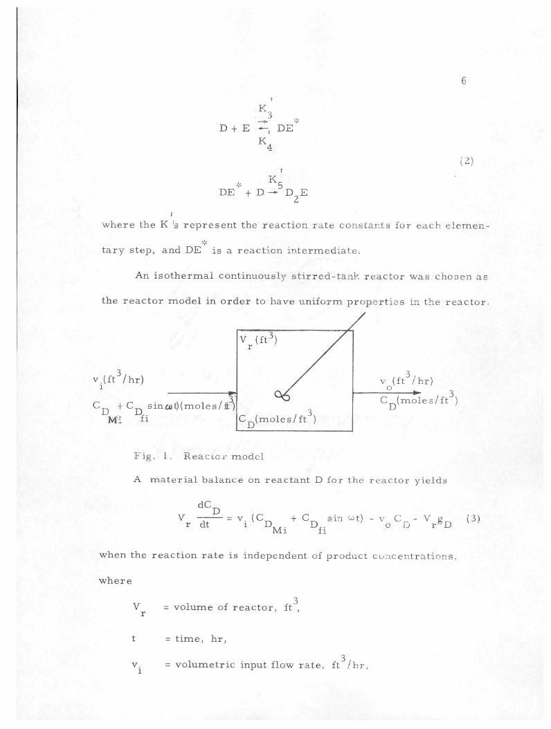
An isothermal continuously stirred -tank reactor was chosen as

the reactor model in order to have uniform properties in the reactor,

v(ft3ihr) v (ft3/hr) o

CD + CD sincyt)(moles/$) CD(moles/ft3)

Mi fi

Fig. 1. Reactor model

A material balance on reactant D for the reactor yields

dCD

Vr dt - vi (CD + CD sin wt) - vo Mi fa

VrbD (3)

when the reaction rate is independent of product concentrations,

where

V r = volume of reactor, ft3,

t = time, hr,

3 vi = volumetric input flow rate, ft3 /hr,

V (ft')

Cr,(moles/ft3)

CU -

3 = mean inlet concentration of reactant D, mores /ft,

CD fi fi

amplitude of input concentration of reactant fi fi D, moles /ft 3

and vo

7

= frequency of the input concentration wave, cycles /hr,

= volumetric output flow rate, ft 3/hr.

Eq. (3) is composed of the molar input flow rate,

vi(CD + CD sin wt), the molar output flow rate, voCD, the molar Mi fi

output by reaction, VrgD, and the accumulation of D in the reactor,

dCD

Vr dt

Further restrictions are imposed on the model to maintain

constant ratios of the reactants if more than one reactant influences

the reaction rate. All reactants are required to flow into the re-

actor with the same frequency and phase angle, and obey the condi-

tion

where .S

and

CD + CD sin wt

Mi fi = S CE + CE sin wt

Mi fi

= stoichiometric ratio of reactant D to E,

(4)

E = mean inlet concentration of any reactant E Mi which influences the rate expression, moles /ft .

w

.

..

.

3

=

CD Mi

0

If v. = v , Eq. (3) can be simplified to1 o

|^= 1+Asinne - ti - f(r]) (5)

by using Eq. (4) and defining the following dimensionless

parameters!

V

ft = w— (6)

e =t^ (?)r

C

ti =pr- (8)

Mi

CDf.A=?r^i (9)

Mi

g Vand f(-n) =-^~JL (10)

CD VMi

The above results hold -when only the reactants influence the

reaction rate. If the product also influences the reaction rate, two

differential equations would be required

-jgl= 1+AsinftG - r\- f(n,v) (11)

dvand — = f(r|, v) - y (12)

where y = ratio of product X in reactor to the mean inputconcentration of reactant D,

and £{r\, y )= f(n) written as a function of both r\ and y .

Total solutions to Eq. (5) consist of a periodic steady-state

component and a transient component, but only the steady-state com

ponent is of interest in the analysis. The transient component in

this analysis is useful only as a means to determine the time re

quired for the process to reach steady-state. The total solution can

be obtained analytically for only three cases, namely, a nonreacting

system, a zero-order reaction, and a first-order reaction (See

calculational methods); otherwise, numerical techniques are re

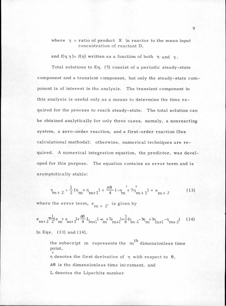
quired. A numerical integration equation, the predictor, was devel

oped for this purpose. The equation contains an error term and is

asymptotically stable:

1 AB ' '•n i_ = -(t1 +n J + —r(-n + 7t1 J + e ., (13)m+ 2 2 'm Wl 4 m 'm+ 1 m+ 2 v '

where the error term, e , is given bym + 2 s '

1 A9 3e , ,-de +e ,)| —L ,(-e +7e ,)+-(ti -3n +3n -ti ) (14)m+2 Z~ m m+1 4 m+1 m m+1 8 m-1 'm m+1 m+ 2

In Eqs. (13) and (14),

the subscript m represents the m dimensionless timepoint,

t

r\ denotes the first derivative of n with respect to 9,

A8 is the dimensionless time increment, and

L denotes the Lipschitz number

10

Solution by this equation becomes impractical for low frequencies

since AO must be increased to obtain the periodic steady -state solu-

tion with a reasonable number of calculations. When L43 is increased,

the error term becomes significantly large and a corrector equa-

tion must then be used in conjunction with the predictor equation.

Another alternative approach requiring only one equation would be

to use the modified Euler's method. Neither of these approaches

were taken since only the periodic steady -state component is of in-

terest and simpler methods are available to compute only this com-

ponent.

Steady -state components.of the total solution can be obtained

by considering an infinite series of some continuous periodic function,

and then determining the constants in this series. The best known

infinite series of a periodic function is the Fourier series. Constants

in this series were determined for a second -order reaction by a trial

and error method. (See Appendix A). This approach was also at-

tempted to evaluate the constants in the Fourier series for a complex

rate equation.

Methods for solving Eqs. (11) and (12) would be the same as

those for Eq. (5) only the computations would be more cumbersome.

These solutions were not attempted because of the exploratory nature

of this work and an initial need to analyze Eq. (5).

11

Numerical and Fourier series solutions to Eq. (5) involved

iteration and, consequently, required digital computers. The com-

putational methods are described in the following chapter.

12

CALCULATIONAL METHODS

In this chapter, several methods for solving Eq. (5) are dis-

cussed. A numerical calculus scheme for determining the total

solution is presented first. Sinusoidal steady -state solutions are

then presented for the three systems that can be solved analytically,

and the Fourier series solutions for other systems where analytical

solutions are not obtainable are expounded. Finally, the possibility

of using an analog computer is discussed.

Numerical Calculus Method

Complete solutions to Eq. (5) were calculated by .Egs.(13) and (14)

on an IBM 1620 digital computer. To start the calculations, values

of p at 0 = 0 and 0 = A0 were required. The initial value of r1 is

arbitrary, being limited to values between zero and one, and the

second is obtained from the initial value using the modified Euler `s

method. Also, error terms corresponding to the first three points

are assigned a value of zero.

Analytic Steady -State Solutions

Analytic solutions of Eq, (5) were obtained for a nonreacting system.

(f(r)) = 0), a zero -order reaction (f(r)) =K), and a first -order reaction

(f(r)) =Kra). The periodic steady -state solutions were as follows:

13

A 1f(n) = 0 t)= 1 + =l sin (06 - tan U) (15)

Vl +n

A 1f(n) = K r] = 1 - K + i sin (^9 - tan ft) (16)

7T a

f(ri) =Kt| ti= + - —sin(fl8 -tan"1 (77-^)) (I7)V(l:-+ K) +Q

Note that in Eq, (16), t; may assume negative values for certain com

binations of K, A and £2. This is physically impossible and arises

from the fact that Eq. (16) predicts a depletion in reactants even

though no reactants maybe present. Therefore, r\ is zero, physically,

whenever negative values are obtained from Eq. (16).

Fourier Series Solution

To obtain the periodic steady-state solution for the second-

order reaction requires a trial and error procedure. First, the

solution is assumed to be a Fourier series, i. e. ,

N

•n=b+T,im "V1'(a sin(U20) + c cos(k«6)) (18)N-'-oo •"•—' k k

k - 1

Experience has shown that the coefficients of the higher frequency

components decrease rapidly with increasing k, and therefore, only

the first five components were considered, i. e. , N was set equal to

five in Eq. (18). When this solution is substituted into Eq. (5) eleven

equations are obtained equating the coefficients of the nonfluctuating

components, the respective sine terms, and the respective cosine terms.

14

These eleven equations are then solved simultaneously by a trial and

error technique on an IBM 1620 digital computer to obtain the con-

stants in Eq. (18). (See Appendix B).

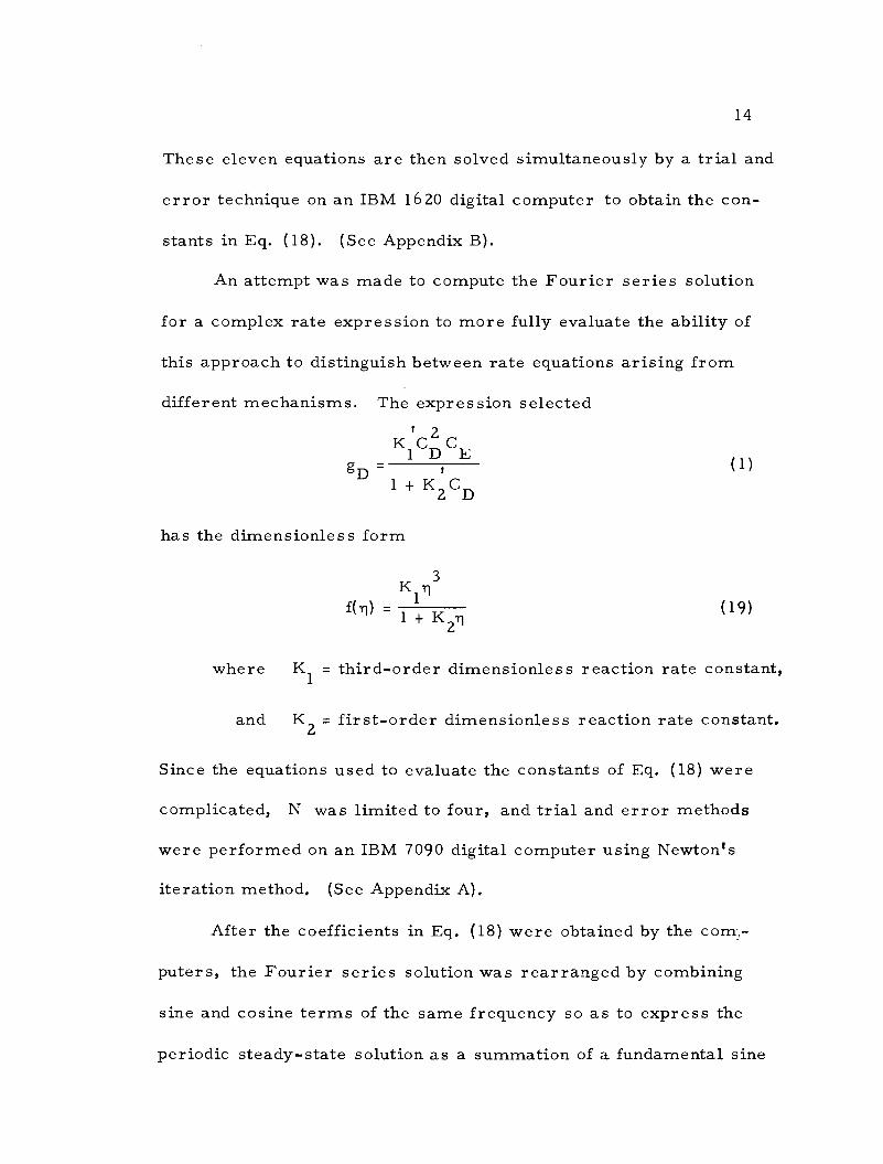
An attempt was made to compute the Fourier series solution

for a complex rate expression to more fully evaluate the ability of

this approach to distinguish between rate equations arising from

different mechanisms. The expression selected 2

K1CD CE gD -

1+K2CD

has the dimensionless form

K 1-1 3

f(n) 1

1+K

2ri

(1)

(19)

where K1 = third -order dimensionless reaction rate constant,

and K2 = first -order dimensionless reaction rate constant.

Since the equations used to evaluate the constants of Eq. (18) were

complicated, N was limited to four, and trial and error methods

were performed on an IBM 7090 digital computer using Newton's

iteration method. (See Appendix A).

After the coefficients in Eq. (18) were obtained by the corn,

puters, the Fourier series solution was rearranged by combining

sine and cosine terms of the same frequency so as to express the

periodic steady -state solution as a summation of a fundamental sine

+ K -

15

wave and its higher harmonics. This was accomplished by the fol-

lowing trigonometric relation (12, p. 260 -262):

// c aksin(kSZO) + ckCos(l O) = ^/ak + c k sin (1(00 + tan -1(ak) )

k

= Ak sin (1(0 -(pk)

where Ak = amplitude of (k - 1)th harmonic,

(20)

and izi)k = phase lag.

Analog Computer Solution

The possibility for using analog computers to obtain solutions

for Eq. (5) was also investigated. Most analog computers are ac-

curate to five percent, but with better components the error could be

lowered to about one percent. Accessories, such as sine wave gener-

tors and servomultipliers, are also available to aid in setting up

fairly complicated expressions. However, since no analog computer

was accessible which had both the sine wave generator and sero-

multiplier and had a precision of one percent, no solutions were at-

tempted.

This method still shows much promise if the desired accuracy

could be obtained, and a servomultiplier and a sine wave generator

were available.

16

DISCUSSION OF RESULTS

In this chaper, the computed responses for nonreacting, zero -,

first- and second -order reaction systems will first be discussed.

Extension to more complicated kinetic systems and experimental con-

siderations will follow.

Nonreacting System

Results showed that the output is sinusoidal and that no change

occurs between the mean input and output concentrations as antici-

pated. The output to input amplitude ratio, -Al, equals 1 and N/1 +52

asymptotically approaches a maximum value of one for small O. The

hase la g,, p equals tan 1S2 and also asymptotically approaches a

maximum of one except for large S2. These results though apparently

trivial, are quite useful since the nonreacting system would be used

for the calibration of recording instruments.

Zero -Order Reactions

Pseudo- steady -state reactions occur in some heterogeneous

catalytic reactions and indicate that a complex reaction is occuring

involving a number of steps. The response curves are identical to

the nonreacting system except that the mean output concentration is

smaller. (See Eqs. (15) and (16) and Fig. (2) ).

A

z

17

10 -2 10 -1 1 10 Dimensionless frequency, SZ

Fig. 2. Amplitude ratio and phase lag for zero -order and nonreacting systems

First -order Reaction

First -order reactions are much more common than zero -order

reactions, examples being radioactive decomposition and decompo-

sition of several gases. Knowledge of any of three response condi-

tions can distinguish a first -order reaction from other rate expres-

sions. For example, both zero- and first -order responses are sinu-

soidal, but the mean output to input concentration ratio,b,varies

1G2

18

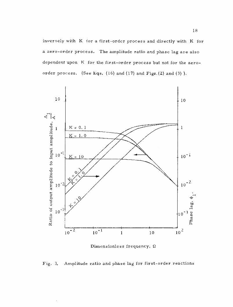
inversely with K for a first -order process and directly with K for

a zero -order process. The amplitude ratio and phase lag are also

dependent upon K for the first -order process but not for the zero-

order process. (See Eqs. (16) and (17) and Figs. (2) and (3) ).

10

K = 0.1

- 10

_ 10 -1

10 -2

10 -1 1 10

Dimensionless frequency, Sl

Fig. 3, Amplitude ratio and phase lag for first -order reactions

19

Second-order Reaction

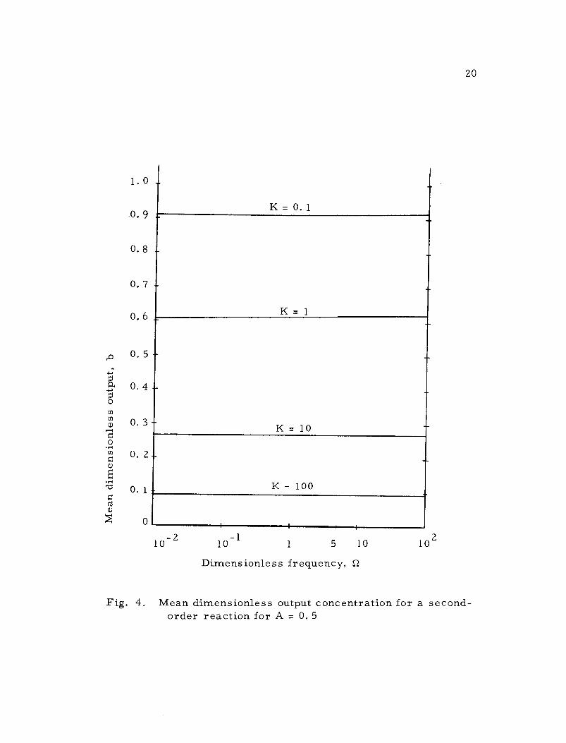
The response to a second-order reaction system differs from

the previous cases in that higher harmonics are present in the out

put wave. Mean output concentrations for a second-order reaction

are different than the first-order response and increase slightly

with increasing £1. (See Eq. (17) and Fig. (4) ). These differences

along with the higher harmonics can be used to distinguish between

first- and second-order rate reactions.

A!Qualitatively, the amplitude ratio — and phase lag cj> for

A 1

a second-order process follow the same pattern with respect to K

and £2 as for a first-order process. However, the second-order

exhibits slightly lower amplitude ratios and phase lags than the first-

order for K<1, whereas wrien'K>10 the difference is more pronounced

and reversed.,(See Figs.. (3) and (5) ).

A2The amplitude ratio —— increases with decreasing £2 and

increasing K for a second-order process and becomes constant at

low frequencies. This behavior is also found in the amplitude ratio

A3—r- with the first harmonic being greater than the second by almost

a factor of ten. (SeeFigs. (6) and (7) ).

Variation in the dimensionless input amplitude, A, has prac

tically no effect on the mean output concentration for £2 > 10. How

ever, when £2 . <10, the mean output concentration is larger for

Mea

n di

men

sion

less

out

put,

b

1. 0

0. 9

0. 8

0. 7

0. 6

0. 5

0. 4

0. 3

0. 2

O. 1

0

K = 0.1 I.

1

1

K = 1

...

K - 10 -

K = 100

,

10 -2 1 5 10

Dimensionless frequency, S2

102

20

Fig. 4. Mean dimensionless output concentration for a second - order reaction for A = 0. 5

-

a

10_1

Rat

io o

f ou

tput

am

plitu

de o

f fu

ndam

enta

l to

-10

21

10 -2

10 -1 5 10

Dimensionless frequency, S2

102

Fig. 5. Amplitude ratio and phase lag of the fundamental for a second -order reaction when A = 0. 5

1

Rat

io o

f fi

rst

harm

onic

to

fund

amen

tal,

10

1

K = 0.1 -10

-1

22

10 -2

10 -1 1 5 10 102

Dimensionless frequency, St

Fig. 6. Amplitude ratio and phase lag of the first harmonic for a second -order reaction when A = 0. 5

K- 1b°

10-4 _

10 -1

lo

Tri

.d 10 C 7

O

E

lo

_

C

3 10

w

K - 10

K = 1. 0

K = 0. 1

x

o

ó 10 -4; ó

.0 á CL

Phas

e la

g of

sec

ond

harm

onic

,

10 _ - lß

10

10 -2 10 -1 1 5 10

Dimensionless frequency, SZ

10

10 -2

10-3

10 -4

10 -5

102

23

Fig. 7 Amplitude ratio and phase lag of the second harmonic for the second -order reaction when A = 0.5

M $

K=0.1

K 10

K=1.0

1

Mea

n di

men

sion

less

out

put,

..0

0. 63

0. 62

0. 01 0. 1 1. 0 10

Dimensionless frequency, 0

100

24

Fig. 8. Mean dimensionless output for various input amplitudes and a second -order K = 1. 0

-

0.61

0. 59

25

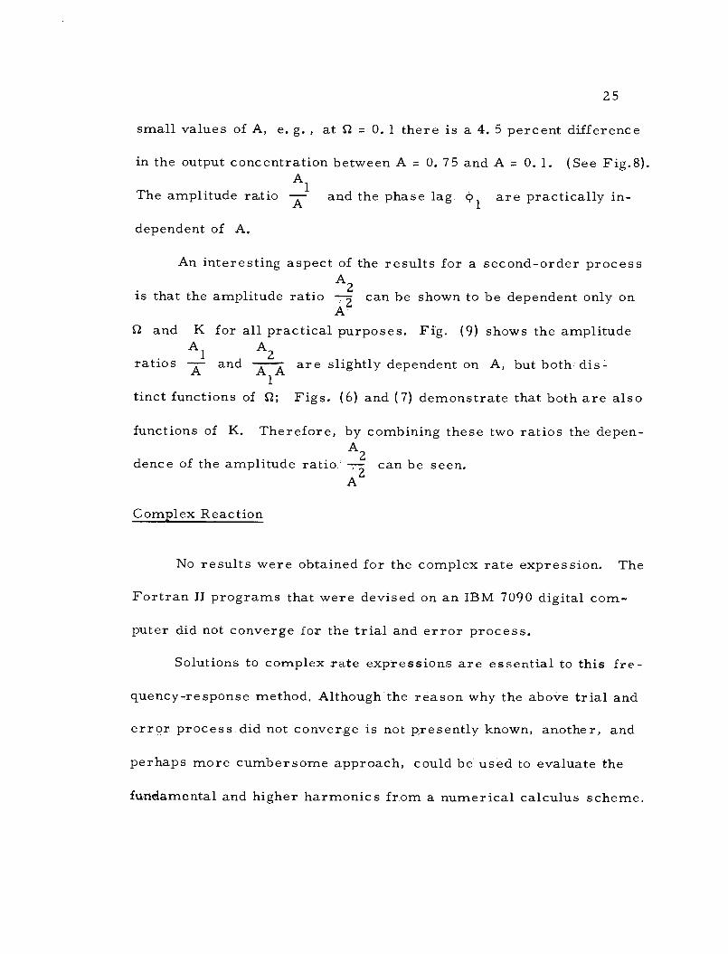
small values of A, e. g. , at S2 = 0.1 there is a 4. 5 percent difference

in the output concentration between A = 0. 75 and A = 0. 1. (See Fig.8). A

The amplitude ratio -Al

dependent of A.

and the phase lag cl)1 are practically in-

An interesting aspect of the results for a second -order process A2

is that the amplitude ratio -2 can be shown to be dependent only on A

S2 and K for all practical purposes. Fig. (9) shows the amplitude Al

ratios X1

and A2A are slightly dependent on A, but both dis- 1

tinct functions of S2; Figs. (6) and (7) demonstrate that both are also

functions of K. Therefore, by combining these two ratios the depen- A

dence of the amplitude ratio. -Z can be seen. A

Complex Reaction

No results were obtained for the complex rate expression. The

Fortran II programs that were devised on an IBM 7090 digital com-

puter did not converge for the trial and error process.

Solutions to complex rate expressions are essential to this fre-

quency- response method, Although the reason why the above trial and

error process did not converge is not presently known, another, and

perhaps more cumbersome approach, could be used to evaluate the

fundamental and higher harmonics from a numerical calculus scheme.

26

A = 0,75

A = O. 1

A 0. 75

A = 0.1

10 -2 10-1 1 5 10 10

Dimensionless frequency, S2

10 -3

Fig. 9. Amplitude ratios with respect to A of fundamental and first harmonic to fundamental for a second - order reaction when K == 1,0

1

-- -

.01

° 10-z

10 -3

27

Numerical Calculus Method

Results of the numerical calculus scheme showed the relia-

bility of Eqs. (13) and (14) and demonstrated that the best choice of

initial conditions to reach the periodic steady -state in minimum time

is the mean output concentration ratio,b. The response curve for a

first -order reaction approached a mean value of O. 500 and an am-

plitude of O. 00980 as predicted by the analytical solution. This first -

order system was studied to test the reliability of the mathematical

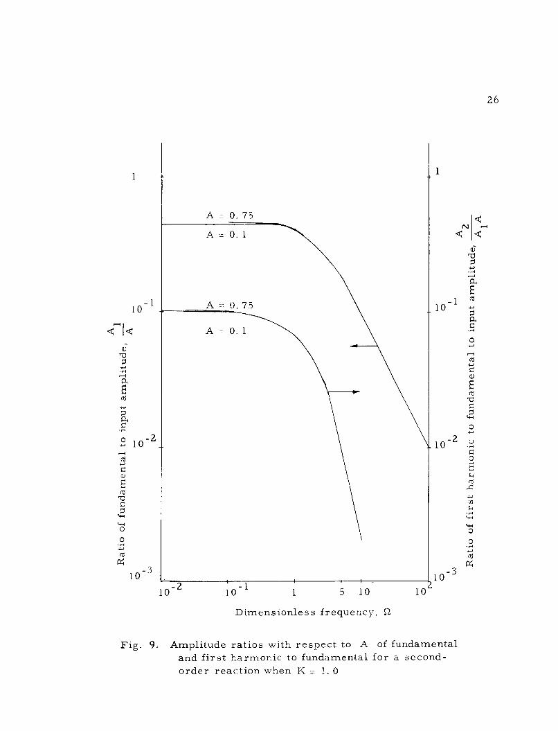
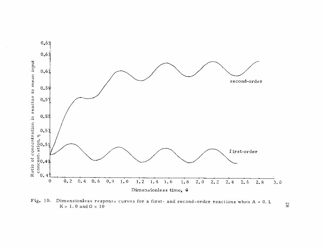
methods. The second -order reaction curve agreed well with the

Fourier series solution and showed the difficulty of observing very

small harmonics when the parameters are S2 = 10, A=0. 1 and K = 1. O.

(See Fig. (10)). The limitations to this method of numerical inte-

gration and other possibilities have been discussed in the theory.

Experimental Considerations

This thesis has been concerned primarily with the theoretical

aspects of frequency- response experiments with chemical reactors.

However, a few comments on the feasibility of conducting experi-

ments are pertinent to this discussion. The experimental task of

producing and analyzing the periodic response and maintaining the

reactor as described in the theory would be difficult at present.

However, with rapid advances being made in instrumentation and

0.6E!

second -order 0.55`

.,

o 0.5:3 0.5-

;-

d ú °0.51 o U - o J o) 0.4(X o ; o gi U

rz 0.4' 0 0.2 0.4 0.6 0.8 1.0 1.2 1.4 1.6 1.8 2.0 2.2 2.4 2.6 2.8 3.0

Dimensionless time, A

Fig. 10. Dimensionless response curves for a first- and second -order reactions when A = 0. 1,

K= 1.0 and S2= 10

ó 0.5'7 u cd a) Ir

0 0.5a-

0

w

a °

0.6

0.6 m

0

first -order

29

analytical techniques, the conduction of experiments as suggested

here is not unreasonable.

The following stipulations must be met:

(1) Input concentration of the reactants must vary in a sinusoidal manner.

(2) Concentration in the reactor must be uniform.

(3) Temperature of the reactor must be constant.

(4) Instruments for continuously measuring the concen- centration must be extremely accurate and have a very small time lag.

(5) The volumetric input flow rate must be equal to the volumetric output flow rate, and both flow rates must be constant.

The theoretical results presented here have demonstrated that

different reaction rate equations do produce a distinctive set of re-

sponse curves. Therefore, assuming that the above mentioned ex-

perimental stipulations can be met, the true reaction rate equation

can be determined by this method.

30

CONCLUSIONS AND RECOMMENDATIONS

This report introduces a method for studying reaction rate

equations. It shows promise because no two different rate equations

have the same response over the complete range of parameter values.

This is especially true at lower frequencies where the higher har-

monics are more pronounced.

In order to increase the scope of this method, additional com-

plex rate equations should be proposed and theoretically analyzed;

then, experiments should be performed to evaluate the practicality

of this method.

31

BIBLIOGRAPHY

1. Black, Harold S. , Stabilized feedback amplifiers. Bell System Technical Journal 13 :1. 1934.

2. Bilous, Olegh, H. D. Block and Edgar L. Piret, Control of con- tinuous flow chemical reactors. A. I. Ch. E. Journal 3:248. 1957.

3. Eigen, M. , Methods for investigation of ionic reaction6s in aqueous solutions with half -times as short as 10 sec. Discussions of the Faraday Society 17:194. 1954.

4. Goheen, Harry E. , Professor of Mathematics. Private Com- munication. Oregon State University, Corvallis, Oregon.

5. Levenspiel, Octave. Chemical reaction engineering. New York, John Wiley and Sons, Inc. , 1962. 501p.

6. Nyquist, H. , Regeneration theory. Bell System Technical Journal 11:126. 1932.

7. Oldenburger, Rufus. Frequency response. New York, Macmillan Company, 1956. 372p.

8. Stelling, P. O. and R. B. M. Elkund, Acceleration of chemical reactions by vibration. Swedish Patent 138, 857. January 27, 1953. (Abstracted in Chemical Abstracts 47:6174h. 1953)

9. Vasil'ev, S. S. and M. S. Selvokhina, The kinetics of nitrogen oxidation in an oscillating discharge. Zhurnal Fizicheskoi Khimi1 32:1299. 1958. (Abstracted in Chemical Abstracts 53:1928 e. 1959)

10. Wight, H. M. , Influence of periodic pressure variations on chain reactions. Planetary Space Science 3:94. 1961.

Ll. Williams, F. A. , Response of a burning solid to small- ampli- tude pressure oscillations. Journal Applied Physics 33: 3153. 1962.

32

12. Wylie, Jr. , C. R. Advanced engineering mathematics. 2nd ed. New York, McGraw -Hill Book Company, Inc. , 1960. 696p.

ak

33

NOMENCLATURE

coefficient of sin (k06) 5..n general periodic steady -state solution of ri

A ratio of amplitude of inlet concentration to mean inlet concentration

Ak dimensionless output of the (k - 1)th harmonic

b mean value of general periodic steady -state solution of ri

c k

coefficient of cos (kS20) in general periodic steady -state solution of ri

CD concentration of reactant D in reactor, moles /ft3

CE concentration in reactor of another reactnt E that influences the rate expression, moles /ft

CD amplitude of inlet concentration of reactant D, moles /ft 3

fi 3

CD mean inlet concentration of reactant D, moles /ft Mi

CE amplitude of inlet concentration of another reactant, E fi that influences the rate expression, moles /ft

CE mean inlet concentration of another reactant, E, that Mí influences the rate expression, moles /ft

em' em+ l' e m + 2

error terms which include truncated and propagated er- rors at m, m + 1 and m + 2, respectively

f(n), f(r',1) dimension less isothermal kinetic rate expressions as a function of 'nand and y, respectively

gD isothermal kinetic rate expression for reactant D as a function of reactants D, E, ... , moles /ft

K, K1, K2 dimensionless kinetic rate constants

Kl

I r

K2' K4

K3' K5

34

third -order rate constant, ft 6 /moles hr 2

first -order rate constant, hr -1

second -order rite constants in mechanism of complex rate equation, ft /moles hr

Lipschitz number evaluated at m + 1 Lm + 1

N an arbitrarily large number in Eq. (18)

S stoichiometric ratio of reactant D to reactant E

t time after reactor started, hr

v., v volumetric input and output flow rates, respectively, ft 3 /hr

o

VR volume of reactor, ft3

Greek Symbols

ratio of concentration of product X in reactor to mean input concentration of reactant D

dimensionless time increment

ratio of concentration of reactant D in reactor to mean inlet concentration of reactant D

lin - 1; %' ñz + 1 in + 2

evaluated at m - 1, m, m + 1 and m + 2, respectively 1 i

in' in + 1 first derivatives of r with respect to O evaluated at m and m + 1 respectively

8 equals tv /VR, dimensionless time

(1)k phase lag of (k - 1)th harmonic

Y

D8

n

35

S2 equals u Vit/v, dimensionless frequency

frequency at which input concentration pulsed, cycles /hr

APPENDICES

APPENDIX A

DIGITAL COMPUTER PROGRAMS

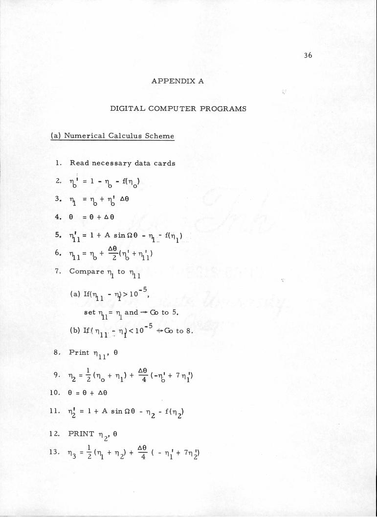
(a) Numerical Calculus Scheme

1. Read necessary data cards

2. y =i - % - f(no)

3. n. = T| + ri1 A01 o o

4. e = e + AG

5. ti* = 1 + A sin £2 6 - ti - f(r) )

6- t\i =tio+ t{ri+r\\]7. Compare n to r\

(a) if(nll - ^>io"5,set ti = ti and -* Go to 5,

(b) If:(ri - r)^<10" *»Goto8.

8. Print r\ , 6

1 AO

io. e = e + AG

11. n' - 1 + A sinne - -n - f(n )

1 2. PRINT r) , 9

1 AG

36

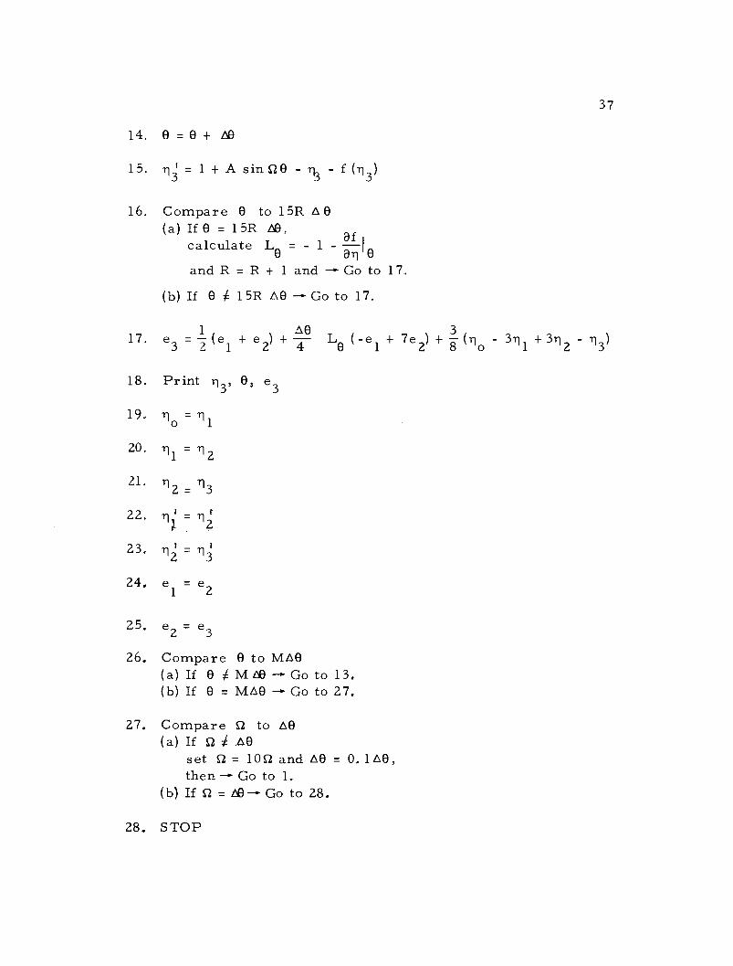
37

14. 0 =0+ oe

15. = 1+A sin SZO -r}3 -f(13)

16. Compare 0 to 15R AO (a) If 0 = 15R A0,

calculate L0 = - 1 -afI

an 0

and R = R + 1 and Go to 17.

(b) If 0 4 15R AO - Go to 17.

17. e3 3

= (el+e2)+ 4 L0(-e1+7e2)+8(rlo- + 2-r13)

18. Print 113, 0, e3

19. 10 =711

20.

21.

22.

23.

24. el = e 2

25. e2 = e3

26. Compare 0 to MAO ( a) If 0 4 M t8 Go to 13, (b) If 8 = MAO Go to 27.

27, Compare S2 to AO

(a) If S2 4 A set S2 = 1052 and AO = 0, 1 A0, then - Go to 1.

(b) If S2 = - Go to 28.

28. STOP

1

T11 =12

38

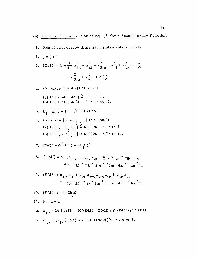
(b) Fourier Series Solution of Eq. (5) for a Second -order Reaction

1. Read in necessary dimension statements and data.

2. j = j + 1

3, (BM2) = 1 - 2 (alk + a2.Q + a3m + a5i + c lk + c 2.2

2 ,2 + c +

c2 + c 4n 5i)

4. Compare 1 + 4K ( BM2) to 0

( a) If 1 + 4K ( BM2) 1 0 - Go to 5.

(b) If 1 + 4K ( BM2) < 0 - Go to 45.

5, bi = ZK( - 1 + 41 + 4K(BM2) )

6. Compare lb. b 1

1,to 0.00001 J

(a) If lb. bj - l

1 0.00001 Go to 7.

(b) If I bj - bj 1 < 0.00001 -; Go to 14.

7. (DM1) = SZ2 + ( 1 + 2b.K)2 J

8. (DM2) = a2.Q c 1k + a3m c

22 + á4n c3m + a5i 4n -a1k c -azec3m-a3mc4n-a4nc5i

(DM3) = a1ka2.Q

+ aa a3ma3ma4n + a4na5i

+ clk c+ c c + c 3m c4n + c4n c5i

10, (DM4) = 1 + 2b,K J

11, k=k+1

12. alk = (A (DM4) - K((DM4) (DM2) + S2 (DM3) ) ) / (DM1)

13. c lk (alk(DM4) - A + K (DM2) )/SZ -- Go to 2,

K

- -

- r -,-

l

9,

*

=

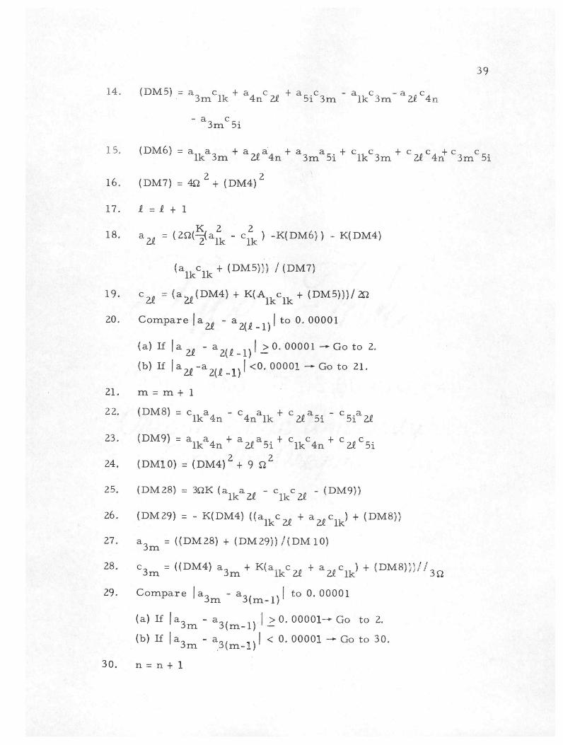
14. (DM5) = a3mclk + d4nc 2Q + a5ic3m - alkc3m- a2F c4n

- a c 3m 5i

15, (DM6) = alka3rn + a 2Q a4n +

16. (DM7) = 4S2 2 + (DM4) 2

17. f = 2 + 1

39

a3ma5i + c1kc3m + c2Qc4ñ c3mc5i

18. a = ( 2S2( ( alk - clk ) -K( DM6) ) - K( DM4)

(alkclk + (DM5))) / (DM7)

19. c 2.2

= ( a ( DM4) + K(Alkclk + (DM5)))/ DM 5) ) ) / 2S2

20. Compare I aa - a2(/ _1)1 to 0. 00001

(a) If I a 2.Q -

a2(1 _1)1> 0. 00001 -- Go to 2.

(b) If I ad -a2(.2

I <0. 00001 --- Go to 21.

21. m = m + 1

22. (DM8) =

23. (DM9) =

clka4n - c4nalk + a5i

alka4n + a2.Qa5i + clkc4n +

24. (DM10) = (DM4) 2 + 9 S22

c5ia2.2

c2Qc5i

25. (DM28) = 3S2K (alkaa - clkc2.2 (DM9))

26. (DM29) = - K(DM4) ((alkc2j2 + a21clk) + (DM8))

27. a3m = ((DM28) + (DM29)) /(DM 10)

= ((DM4) a 3m + K(a c 1k

+ a c ) 2P lk )'` + (DM8);¡// 28. c3m

2Q 3S2

29. Compare I a3m -

a3(m-1)1 to 0. 00001

(a) If I a3m

- a3(m-1) I ? 0. 00001--; Go to 2.

(b) If I a3m - á3(m-1) I

< 0. 00001 -4- Go to 30.

30. n=n+1

-

-

-

40

31. (DM11) = a c, + a c . + a„ cin + ac.c - a.. c_, .Ik 3m 21 21 3m Ik 5i Ik Ik 5i

32. (DM13) = a,.a,, + c,.c5i Ik 5i Ik

33. (DM14) =^(a^ - c^)

34. (DM15) =(DM4)2 + l6n2

35. a. = K( -(DM4) (DM 11) + 4i2((DM14) - (DM13))) / (DM15)4n

36. q4 =((DM4)a4 +K(DMll))/4fi

37. Compare la,, - a,. n.| to 0. 000014n 4(n - 1)'

(a) If la. -a.. ,. | ^- 0. 00001 —Go to 2.4n 4(n - 1)

(b)If|a, - a„, ,.| < 0.00001 —Go to 38.4n 4(n - 1)

38. i = i+ 1

39. (DM16) = a c.,+ a, c_, + a c + a_,c.4n Ik 3m 21 21 3m Ik 4n

40. (DM17) = re. + c-.-c, -a a -a aIk 4n 21 3m Ik 4n 2£ 3m

.

41. (DM 18) =(DM4)2 + 25 fi2

42. a_. = ( - K ((DM 16) (DM4) +5(DM17)J2)) / (DM18)31

43. c _. = ( (DM4) a.. + K(DM 16)) / 5nDl 31

44. Compare Ia_. - ar/. ,.| to 0.000015i 5(i - 1)

(a) If |a_. -a... , J - 0. 00001 —Go to 2.5i 5(i - 1)

(b) If |ac. - ac/. ,. I < 0. 00001 — Go to 45.5i 5(i - 1)

45. Print b., a^, c^, a^, c^, a3m

46. Print c3m> a^, c^, a,.., Cg.. c5(. _„

47. Print c., ,., c-0/ ,v k, i, m, n, i, j — Go to 1.4(n - 1) 3(m - 1)

41

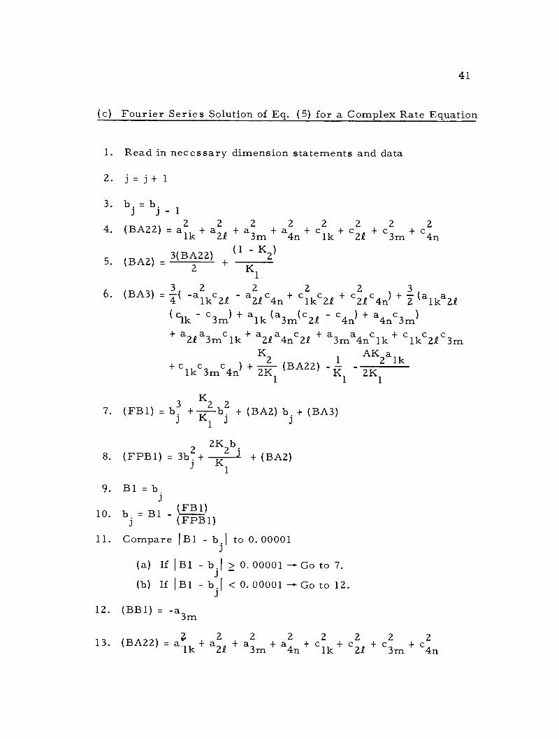
(c) Fourier Series Solution of Eq. (5) for a Complex Rate Equation

1. Read in necessary dimension statements and data

2. j = j + 1

3. b. = b, J J - l

2 2 4. (BA22) = alk + a2Q + a3m +

2

a4n + clk + c2Q + c3m + c4n (1 - K )

5. (BA2) - 3(B222) K

2

1

6. (BA3) - 3 2 2 2 2 3

- ( -a1kc2Q - a2,2 c4n + c1kc2Q + c2,Q c4n) + (a1ka2,Q

(9.k - c3m) + alk (a3m(c21 - c4n) + a4nc3m)

+ a2.Qa3mclk + a2.Qa4nc2.12 + a3ma4nclk + c1kc2.Qc3m K2 AK2alk

+ clkc3mc4n) + 2K1 (BA22) - Kl

K 7. (FB1) = b +

K2 b + (BA2) bj + (BA3)

1

2K b 8. (FPB1) = 3b + K + (BA2)

1

9. B1 =b .l

10. b = B1 - .l

(FB1) (FPB1)

11. Compare 1B1 - b, i to 0. 00001 J

( a) If 1B1 - 13,1 > 0. 00001 Go to 7. - (b) If I B1 - bjI < 0.00001 Go to 12.

12. (BB1) = -a3m

13. (BA22) = a lk + a2Q + a3m + a4n + clk + c2Q + c3m + c4n

2

J

J

2K1

42

14. (BB2) = 2 (2b - 2bjc21 21

+ (BA22) - alk - a21 a4n - c22 c4n

2 -clkc3m 3K (S2a2,Q -4b.+2c2+2-K ) )

1 J 2

15. (BB3) = 4bj (a2.2 clk - a2.Q c3m + a3mc2.Q - a3mc4n+ a4nc3m) 2 2 2

+ a3m(a21 + clk -C ) + 2(a2.Q (a3ma4n+ c2.Q c3m+ c3mc4n)

+ a3mc2.Q a4nc1kc2R c4n+

- a2.2 clkc4n - a4nc2.Q c3m) 42c 2K 0

2

3K 3K (LID jc 1k+ a2/ a3m+a 4ri c lkc2.2

1 1

4 +

c2.2 c3m+ c3m c4n) + 3K1 (a2 .Q

ka, -

a21 c3m+ a3mc2.Q

K - a3mc 4n+ 3m a4nc - A ( 1+K2b.- 2c2Q

) ) J

16. k=k+ 1

17. alk = al(k - 1)

18. clk = c1(k - 1)

19. (FA1) = alk + (BB1)alk +(BB2)alk + (BB3)

20. (FPA1) = 3alk + 2(BB1)alk + (BB2)

21. All = alk (FA1) 22. alk = All- (FPA1)

23. Compare I All - alkl to 0. 00001

(a) If IAll - a1kl Z 0. 00001 -- Go to 19.

(b) If IAll - alkl < 0. 00001 Go to 24.

24.. (BC1) = c3m

K2

clk

-

43

25. (BA22) = al2 2 2 2 2 2 2 2

k+ a 2 + a3m+ a4n+c1k+ cif + c3m+ c4n

2 a

26. (BC2) = 2(2b?+(BA22) - 2 -clk+alka3m+a2Qa4n J

2K

2 a/ +c2c4n 3K (S2alk -SZ2 -K ,2

+ 1 -b.- c2/) 1 2 J

27. (BC3) = 4bj(a1ka2.2+a2.Qa3m+a3ma4n+clk+c2.Qc3m+c3mc4n) a c at

- alkc3m+ 2alk( -a2.Q c4n+ a4nc2Q )+ 2a2 (- 3m

2

+ a3mc2.Q - a3mc4n+ a4nc3m) + 2c2,Q (a3ma4n c3m

2

2K2S2 talk + c3mc4n)

+ 3K1 ( + 2b.alk

- a2/ c3m - a3mc4n

4K 2

+ a 1kc2.Q + a3mc2.Q +a4nc3m) + 3K (alka2.2 + a2.Q a3m

Aa2/ + a3ma4n+

c21 c3m+ c3mc4n 2

28. (FC1) = lk + (BC1) + (BC2) cik clk+ (BC3)

29. (FPC1) = 3cik + 2(BC1) clk + (BC2)

30. C11 = clk

32. Compare IC11 - c1kl to 0.0001

(a) If I C11 C11 - clkl ? 0. 00001 - Go to 28.

(b) If I C11 - clkl < 0. 00001 - Go to 33.

33. Compare k to 4 (a) If k? 4-Go to 34. (b) Ifk<4-Goto 12.

2

g2

34. Compare 1 clk - c1 (k - 1) 1 to 0. 00001

(a) If 1 clk - cl(k - l) 1

0. 00001 - Go to 2.

(b) If 1 c - 1) 1 < 0. 00001 -- Go to 35.

35. (BA22) = alk + a2/ + a3m + a4n + clk + c2.2 + c3m + c4n

36. (BD2) = 2 ( (BA22) - a21 -

2

c2.Q 2 + 2b (b3. - c4n) + a 1 ka3m

c

3K ( a4n K + 1 - 2b. +K n)

1 2 3

2

37. (BD3) = 2 (2bi(alkclk - a1kc3m + a3mclk+ a4nc21 )

+ alk ( a a + c c + c c a3ma4n

lk a3ma4n 22 c3m c3mc4n) )+ a3m( 3m 3

2 ¡ alk c'lk

+ C 1kc2/ +

) + a + a4n ( 2

+ 2 clkc3m)

- clk( a2.2 c3m + a3mc4n + alkc4n )

2

a3mc4n 6

2 2

a4nc3m clk

- + 2 2 + clkc3m + c2. c4n)- alkclk Ac lk

+ alkc3m - a3mclk - a4nc2.Q + 2

38. .2 =.Q +1

39. 2.Q = a 2(.Q - 1)

40. c2/ = c2(1 - 1)

41. (FA2) - a2.2

+ (BD2) a2/ + (BD3)

42. (FPA2) = 3a2 + (BD2)

43. A22 = a2/

44

- cl(k

-

+

2 Z 2 2 2 2 2 2

- )

45

45. Compare 1A22 - a2ß 1 to 0. 00001

(a) If 1A22 - a2ß I ? 0. 00001 --- Go to 41.

(b) If 1A22 - a2ß 1 < 0. 00001 -- Go to 46.

46. (BA22) = alk +a 2/ + a3m a4n+ c lk + c2ß +c3m +c4n

2 a

47. (BE2) = 2 (2b + 2bjc4n + (BA22) - 22ß - c2ß - alka3m

2K c

+ clkc3m + 3K1 (a4n + - 1 + 2n)

2 2

48. (BE3) = 413i ( alk

+ 2 +a lk 3m a

+ a 4n + clkc3m c )

2

alkc4n + 2alk( - + a4nclk+ a2ßc3m) + 2a3m(a2ßclk

a3mc4n - + a4nc3m

+ alkc4n + a4nclk) + 2( - alka4nc3m

clkc4n 2 8 a2ß +clk ( c3mc4n + 2 ) ) + c3mc4n + 3K1

4K ( SZ (2bja2ß + alkclk

- alkc3m - a2ß c4n - a3mclk )

2 2

a1k clk +a a +a a +c c 2 2 2ß 1k 3m 22 4n lk 3m

A +_2

( a1k - a3m + c3m) )

49. (FC2) = c + (BE2) c2P (BE3)

50. (FPC2) = 3c2ß + (BE2)

51. C22=c.2ß

52. c =C22 - (FC2) 2 ß (FPC2)

K2 1 2

+

)

- a2P

lk

Z

- + +

46

53. Compare 1C22 - c I

to 0. 00001

(a) If IC22 - c I ? 0. 00001 -- Go to 49.

(b) If 1C22 - c I

< 0. 00001 Go to 54.

54. Compare to 4 (a) If ,Q ? 4 G to 55. (b) If .Q < 4 Go to 46.

55, Compare I c2/ - c2(1 1 to 0. 00001

(a) If I c - c2(/ I

? 0. 00001 -- Go to 2.

(b) If I c - c2(/ I

< 0. 00001 -- Go to 56.

56. (BA22) = a 2 2 2 2 2 2

+ ale + a3m + a4n + clk + c2P + c3m + c4n

c4n

c 2

57. (BF2) = 3 ( 2b . + (BA22) - a2 3m + a a - c c )

3m 2 2 4n 2Q 4n

+ K2(4b, + K

- 2) 1

j 2

58. (BF3) = 6bß c -a c +a c + a c lk 2Q alkc4n+ a21 clk + a4nclk) -

2 2

+ alk2lk

+ 3alk(a2.Qa4n + c2.Qc4n +

-2 )

3

alk 2

+ 3a2Q (c1kc2.Q + c3mc4n) + 3a4n(c1kc2Q

+ c2.Qc3m) 2

2 3a1kc2Q 6S2 c3m

+ alkclk - 3a2.Qclkc4n

3K2

2 K1

S2 ( - 2b .c -aa4n + lk a1k a2Q lk 4n -cc 3m

2K2 -clkc2)

+ K1 ( a1kc2.Q . - alkc4n + a2.Qclk

A + a4nclk

+ 2 ( - c2/ + c4n) )

.2

1)

+ K1

1)

59. m = m + 1

60. a = a3m 3(m - 1)

61. c = c3m 3(m - 1)

62. (FA3) =a.1 + (BF2) a + (BF3)3m 3m

63. (FPA3) =3a2 + (BF2)3m

64. A33 = a,3m

65 a -A33 (FA3)bb' a3m " A33 (FPA3)

66. Compare |A33 - a„ I to 0. 000013m

(a) If |A33 - a, I > 0. 00001 —Go to 62.3m

(b) If IA33 -a, I < 0. 00001 —Go to 67.3m

222 2222 267. (BA22) = a + a + a + a + c + c + c + c

Ik Zx 3m 4n Ik Zx 3m 4n

2

68. (BG2) =2(2b2+ BA22) - c\ -^- - a..a, +c9,c.j 3m 3 Zx 4n Zx 4n

2K2 1+3K; <K^ "1+2V>

69. (BG3) =f (3b. ( -aika2i +a^t c^ +c^3

- — a (a c + a c a. c_.) ) + 2a.2 Ik 2i Zx Zi 4n — 4n ZV 4n

c

/ v Ik . 2 2 ,(a c +a c +~T -au + cn + 6co»c^2i Ik 3m 2i 3 Ik Ik 2i 4n

,2 _ 2 . , _ . 2a,"3a2i -3c2i)+2a3m(a2iC4n+ K^_

47

48 4K2S2

+ 3K1 (3bja3m +alkclk+ 2 ( alkc4n +a2,Qc1k

a1kc2.Q 4K2 + a4nclk

+ 3 ) ) +3K1 ( - a1ka2Q +alka4n

A + clkc2.2 + clkc4n + 2 (a2.Q

- a4n))

70. (FC3) = c3m + (BG2) cam + (BG3)

71. (FPC3) = 3c3m + (BG2)

72. C 33 = c 3m

74. c =C33 - (FC3) (FPC3)

75. Compare 1C33 - c3ml 3m

to 0. 00001

(a) If IC33 - c3m1 ? 0. 00001 -i Go to 70.

(b) If 1C33 - c3m1

< 0, 00001 - Go to 76.

76. Compare m to 4

(a) If m 4 -- Go to 77. (b) If m < 4 - Go to 56.

77. Compare I c3m - c3(m 1) I to 0. 00001

(a) If 1 c3m - c3(m - 1) 1 0. 00001 - Go to 2.

(b) If I c3m - c3(m 1) I

< 0. 00001 --- Go to 78.

78. (BA22) = a2 + a2 + a2 + a2 + c2 + c2 + c2 + c2 lk 2.Q 3m 4n lk 2.Q 3m 4n

c2 K 79. ( BH2) = 2(3b. +

Z ( ( BA22) - a4n - Z n ) +

K2 (-1 - 1 + 2b.) )

1 2

80. (BH3) = 2(3b (a c +a c +a c 3alk a1ka2Q lk 3m 2/ 2.Q 3m lk) 2 ( 2

?

-

_

1

3m

49

2 2

(c +c1kc22 ) ) + 3a2.2k + alka3m + c1kc3m +

a

3 )

3 2 + 3a3m(clkc2.

+ c2.Qc3m) - 3a1kc2.Qc3m^k 2a21 c3m 2

- a3 2c4n

-

8 Kc4n +

2 (4S2( - 2b

.c4n + alka3m 1 1

2 2

+ 2

c2P

- clkc3m ) ) + 2K2 (alkc3m + a2,2c2.Q

1

Ac 3m

+ am - 3c lk 2

81. n = n + 1

82. a4n - a4(n - 1)

83. c4n - c4(n - 1)

c4n 84. (BH1) - 2 85. (FA4) = a4n + (BH1) a4n + (BH2) a4n + (BH3)

86. (FPA4) = 3a4n + 2(BH1) a4n + (BH2)

87. A44=a4n

88. a4n = A44 - (FA4) ( FPA4)

89. Compare 1A44 - a4n1 to O. 00001

(a) If 1A44 - a4ñ1 ? 0. 00001 -- Go to 85.

(b) If 1A44 - a4n1 < 0. 00001 Go to 90.

2 2 2 2 2 2 2 90. (BA22) = alk + a21 + a3m + a4n + clk + c2P + c3m + c4n

a2.Q

2

- 2

50

2

91. ( BI2) = 2 ( 2b + ( BA22) - a3n - c4n + 3K2 ( K 1

- 1 + 2b ,) )

1 2

92. (BI3) = 2b.( - a2.Q c2.2

- 2alka3m + 2cikc3m) + 2alk J

2 (a21 c3m + a3mc21 - a2.Q c ik) +

c 1kc2.Q + 2( -a2.Q a3mc lk 2

c c 2 +

c1kc2.Q c3m) - a1kc2.Q + 2(a2,Qa3m m c3 +

22 3m

2 3 2 a2.ea3m a4n a3mc2.e 8SZa4n 4K2

+ + ( 6 6 3 3K 3K 1 1 1

2S2(2ba4n + alkc3m +a 2c2 +a

c 3mlk) 2 2

- a2/ +

c2 2 -alka3m

+ c1kc3m +

A 23m

93. (FC4) = c4n + (BI2)c4n + (BI3)

94. (FPC) = 3c42n + (BI2)

95. C44 4n

(FC4) 96. c4n = C44 - ( FPC4)

97. Compare IC44 - c4n1 to O. 00001

(a) If 1C44 - c4n1 ? 0. 00001 -- Go to 93.

(b) If 1C44 - c4n1 < O. 00001 - Go to 98.

98. Compare N to 4 ( a) If N ? 4 -- Go to 78, (b) If N< 4 Go to 99

99. Compare I c4n - c4(n _ 1) I

to 0. 00001

(a) If I c4n - c4(n I

0. 00001 Go to 2.

(b) If I c4n c4(n - 1) I

< O. 00001 -- Go to 100.

+

+

-

] 1

-

51

100. Print bj, alk' c lk' a2.Q' c22 ' a3m' c3m' a4n' c 4 101. Print j, k, Q , m, n

,

52

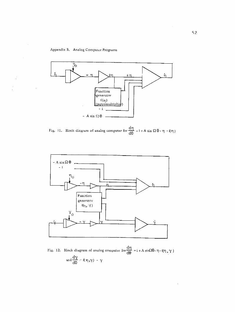
Appendix B. Analog Computer Programs

e +11

Function ?generator

f(n) ( servomultiplie;

- A sin Q O

Fig. 11. Block diagram of analog computer for d8

=1+ A sin S-2 O - 1 - f(TI )

-A sin SZ6

-1

Function generator

f( ?I, Y)

Y

Fig. 12. Block diagram of analog computer for- =1 + A sin 2e -1) - f(T +( )

and dé = f(Tl ,Y) - Y

0

-T1

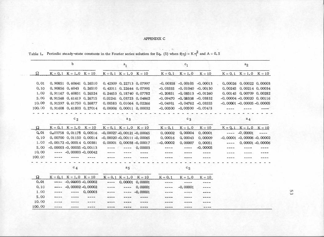
APPENDIX C

Table L. Periodic steady-state constants in the Fourier series solution for Eq. (5) when f(r|) = Kr| and A = 0.5

a K = 0.1 K= 1.0 K= 10 K=0.1 K=1.0 K = 10 K s 0. 1 K = 1.0 K=10

0.01 0.90851 0.60641 0.26510

0.10 0.90856 0.6043 0.26510

1.00 0.91167 0.60851 0.26524

5.00 0.91568 0.61619 0.26715

10.00 0.91597 0.61750 0.26877

100.00 0.91608 0.61803 0.27014

0.42309 0.22713 0.07997 -0.00358 -0.00105 -0.00013

0.42011 0.22644 0.07995 -0.03555 -0.01040 -0.00130

0.24653 0.18740 0.07782 -0.20851 -0.08513 -0.01260

0.02241 0.03723 0.04862 -0.09470 -0.08338 -0.03832

0.00583 0.01064 0.02266 -0.04931 -0.04762 -0.03555

0.00006 0.00011 0.00032 -0.00500 -0.00500 -0.00423

SL K = 0. 1 K=1.0 K = 10 K = 0. 1 K=1.0 K = 10 K = 0.1 K=1.0 K=10

CL01

0.10

1.00

5.00

10,00

100. 00

Q

0.01

0.10

1.00

5.00

10.00

100. 00

0*00758 0.01178 0.00516.

0.00700 0.01150 0.00514

-0.00172-0.00014 0.00381

-0. 00003 -0.00035 -0.00113

-0.00003-0.00042

-0.00027 -0. 00121 -0.00065

-0. 00020 -0. 00111 -0. 00065

0.00001 0.00038-0.00017

0.00003

K = 0.1 K=1.0 K=10 K = 0.1 K = 1.0 K = 10

— -Gi 00003 -0. 00002

—-- -0.00002-0.00002

0.00003

-- 0.00001 0.00001

0.00001

0.00001

0.00002 0.00004 0.00001

0.00016 a 00043 0.00009

-0.00002 0.00007 0.00051

-0.00005

K = 0. 1 K = 1.0 K=10

-0. 00001

K = 0. 1 K=1.0 K = 10

0,00026 0.00022 0.00003

0.00245 0.00214 0.00034

0.00145 a 00709 0.00282

-0. 00004 -0. 00020 0. 00116

-0. 00001 -0. 00005 -0. 00005

K = Q. 1 K=1.0 K=10

-0.00001

-0.00001 -0. 00006 -0. 00002

0. 00001 -0. 00006

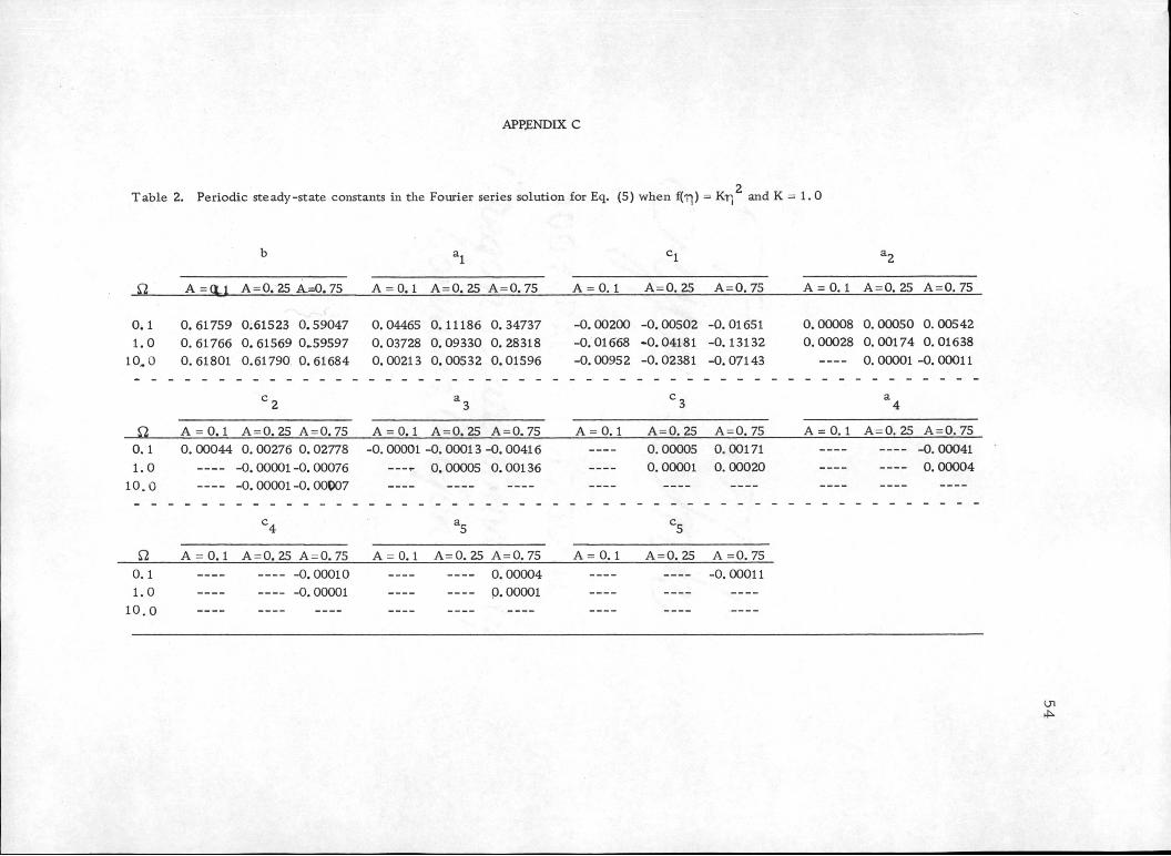
APPENDIX C

Table 2. Periodic steady-state constants in the Fourier series solution for Eq. (5) when f(r>) = Kr, and K = 1. 0

_0_ A=cy A=0. 25 A=0. 75 A = 0.1 A=0. 25 A=0. 75 A = 0. 1 A= 0. 25 A=0. 75 A = 0. 1 A=0. 25 A=0. 75

0.1 0.61759 0.61523 0.59047

1.0 0.61766 0.61569 0.59597

10.0 0.61801 0.61790 0.61684

0.04465 0.11186 0.34737

0.03728 0.09330 0.28318

0.00213 0.00532 0.01596

SL A = 0.1 A = 0. 25 A = 0.75 A = 0.1 A = 0. 25 A = 0.75

0. 1 0. 00044 0. 00276 0. 02778

1.0 -0.00001-0.00076

10.0 -0.00001-0.00007

-0. 00001 -0. 00013 -0. 00416

—— 0.00005 0.00136

a A = 0.1 A = 0. 25 A = 0. 75 A = 0.1 A=0.25A=0.75

0.1

1.0

10.0

0.00010

0.00001

0. 00004

0. 00001

-0.00200 -0.00502 -0.01651

-0.01668 -0.04181 -0.13132

-0.00952 -0.02381 -0.07143

A = 0.1 A = 0. 25 A = 0. 75

0. 00005

0. 00001

0.00171

0. 00020

A =0.1 A = 0. 25 A =0.75

-0.00011

0.00008 0.00050 0.00542

0.00028 0.00174 0.01638

0.00001-0.00011

A = 0.1 A = 0.25 A = 0.75

-0. 00041

0. 00004

4^