Chemistry 362 Dr. Jean M. Standard

Problem Set 4 Solutions

1. The two-dimensional particle in a box model can be used to estimate the energy levels of the porphyrin molecule shown below.

Assume that the two-dimensional box is a square of approximately 7 Å on each side. The conjugated portion of the porphyrin molecule consists of 18 pi electrons. Calculate the energy of the highest occupied molecular orbital (HOMO) and the lowest-unoccupied molecular orbital (LUMO) in Joules. Calculate the wavelength in nanometers of a transition from the HOMO to the LUMO for the porphyrin molecule.

Treating the porphyrin molecule as a two-dimensional box gives energy levels of the form:

€

Enx ,ny = nx2h2

8mL2 + ny

2h2

8mL2 .

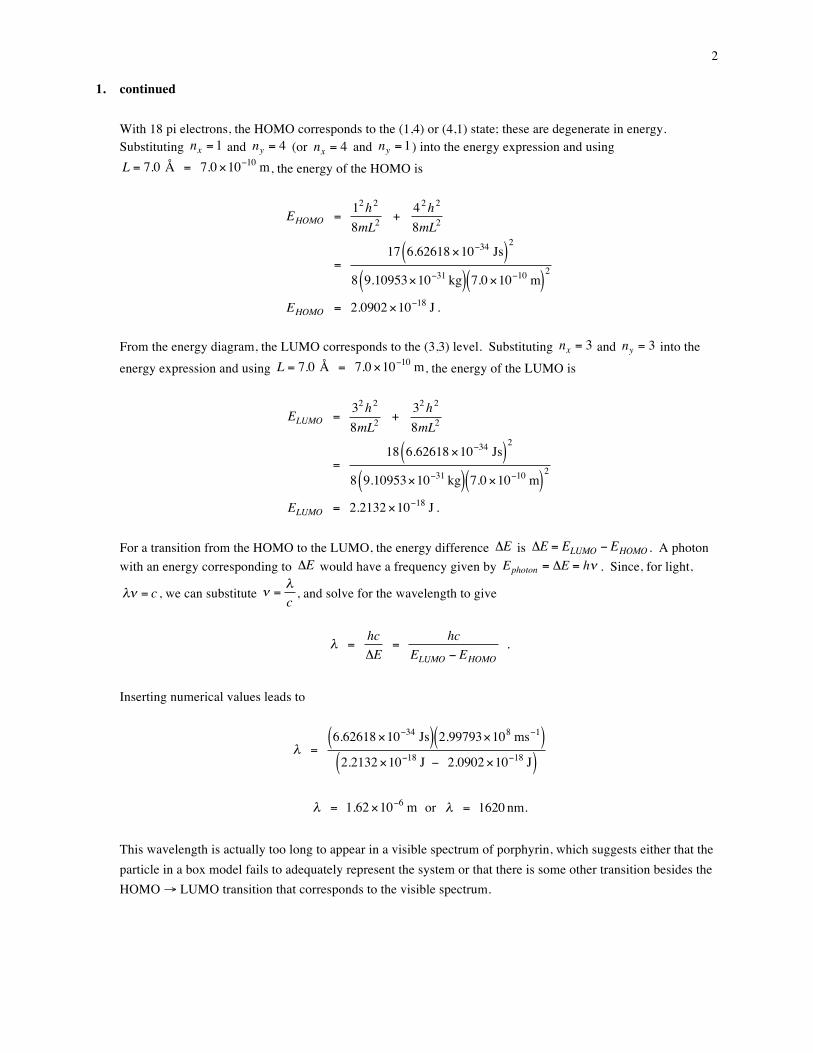
where L is the length of one side. The energy level diagram for this two-dimensional box would look something like that shown below.

aa

NH

NN

HN

(nx, ny)

(1,2) (2,1)

(1,1)

(2,2)

(1,3) (3,1)

(2,3) (3,2)

(1,4) (4,1)(3,3)

(2,4) (4,2)

(3,4) (4,3)

2

1. continued

With 18 pi electrons, the HOMO corresponds to the (1,4) or (4,1) state; these are degenerate in energy. Substituting

€

nx = 1 and

€

ny = 4 (or

€

nx = 4 and

€

ny = 1) into the energy expression and using

€

L = 7.0 Å = 7.0×10−10 m, the energy of the HOMO is

€

EHOMO = 12h2

8mL2 + 42h2

8mL2

= 17 6.62618×10−34 Js( )2

8 9.10953×10−31 kg( ) 7.0×10−10 m( )2

EHOMO = 2.0902×10−18 J .

From the energy diagram, the LUMO corresponds to the (3,3) level. Substituting

€

nx = 3 and

€

ny = 3 into the energy expression and using

€

L = 7.0 Å = 7.0×10−10 m, the energy of the LUMO is

€

ELUMO = 32h2

8mL2 + 32h2

8mL2

= 18 6.62618×10−34 Js( )2

8 9.10953×10−31 kg( ) 7.0×10−10 m( )2

ELUMO = 2.2132×10−18 J .

For a transition from the HOMO to the LUMO, the energy difference

€

ΔE is

€

ΔE = ELUMO − EHOMO . A photon with an energy corresponding to

€

ΔE would have a frequency given by

€

Ephoton = ΔE = hν . Since, for light,

€

λν = c , we can substitute

€

ν =λc , and solve for the wavelength to give

€

λ = hcΔE

= hcELUMO − EHOMO

.

Inserting numerical values leads to

€

λ = 6.62618×10−34 Js( ) 2.99793×108 ms−1( )

2.2132×10−18 J − 2.0902×10−18 J( )

€

λ = 1.62×10−6 m or

€

λ = 1620 nm. This wavelength is actually too long to appear in a visible spectrum of porphyrin, which suggests either that the particle in a box model fails to adequately represent the system or that there is some other transition besides the HOMO → LUMO transition that corresponds to the visible spectrum.

3

2. For the two-dimensional model of porphyrin described in problem 1, determine the wavelength in nanometers of a transition from the HOMO to the LUMO+1 for the porphyrin molecule. Which transition, the HOMO → LUMO or HOMO → LUMO+1 falls in the visible range of the spectrum? The energy of the HOMO is the same as in problem 1, so the only energy that we need to calculate is the LUMO+1 energy. From the energy diagram given in problem 1, the LUMO+1 corresponds to the (2,4) or (4,2) level. Substituting

€

nx = 2 and

€

ny = 4 into the energy expression and using

€

L = 7.0 Å = 7.0×10−10 m, the energy of the LUMO+1 is

€

ELUMO+1 = 22h2

8mL2 + 42h2

8mL2

= 20 6.62618×10−34 Js( )2

8 9.10953×10−31 kg( ) 7.0×10−10 m( )2

ELUMO+1 = 2.4591×10−18 J .

For a transition from the HOMO to the LUMO+1, the energy difference

€

ΔE is

€

ΔE = ELUMO+1 − EHOMO . A photon with an energy corresponding to

€

ΔE would have a frequency given by

€

Ephoton = ΔE = hν . Since, for

light,

€

λν = c , we can substitute

€

ν =λc , and solve for the wavelength to give

€

λ = hcΔE

= hcELUMO+1 − EHOMO

.

Inserting numerical values leads to

€

λ = 6.62618×10−34 Js( ) 2.99793×108 ms−1( )

2.4591×10−18 J − 2.0902×10−18 J( )

€

λ = 5.39×10−7 m or

€

λ = 539 nm. The wavelength of the HOMO → LUMO+1 transition does correspond to a transition in the visible region of the spectrum. The HOMO → LUMO transition calculated in problem 1 does not.

4

3. Consider an electron trapped in a three-dimensional square box of length L on each side.

a. By analogy with the two-dimensional case, give the equation for the quantized energy levels of the particle in a 3D box. What is the form of the wavefunction?

By analogy with the 2D case, we will need three quantum numbers (one for each dimension, nx , ny , and nz ) to describe the energy levels of the particle in a 3D box,

Enx ,ny ,nz  =   nx2h2

8mL2  +  ny

2h2

8mL2    +  nz

2h2

8mL2 ,

where L is the length of one side. Similarly, the wavefunction will be represented as a product of three one-dimensional terms,

ψnx ,ny ,nz (x, y, z)   =   2L!

"#

$

%&

3/2

sin nxπ xL

!

"#

$

%&  sin

nyπ yL

!

"#

$

%& sin nzπ z

L!

"#

$

%& .

b. What is the expression for the energy of the ground state of the electron in the 3D box?

From part (a), the energy levels of the particle in a 3D box are

Enx ,ny ,nz  =   nx2h2

8mL2  +  ny

2h2

8mL2    +  nz

2h2

8mL2 .

The lowest quantum number in each direction is 1, so substituting nx =1 , ny =1 , and nz =1 into the expression yields the ground state energy, E111 ,

E111  =   12h2

8mL2  +  12h2

8mL2    +  12h2

8mL2 ,

or      E111  =   3h2

8mL2 .

c. Give the quantum numbers for the first excited state of the electron in a 3D box. What is the

degeneracy of the first excited state?

The first excited state would correspond to increasing only one of the three quantum numbers from 1 to 2. There are three possible ways to do this: nx, ny, nz( )  =   1, 1, 2( )  or    1, 2, 1( )   or    2, 1, 1( ) . Thus, we say

that the degeneracy of the first excited state is three.

5

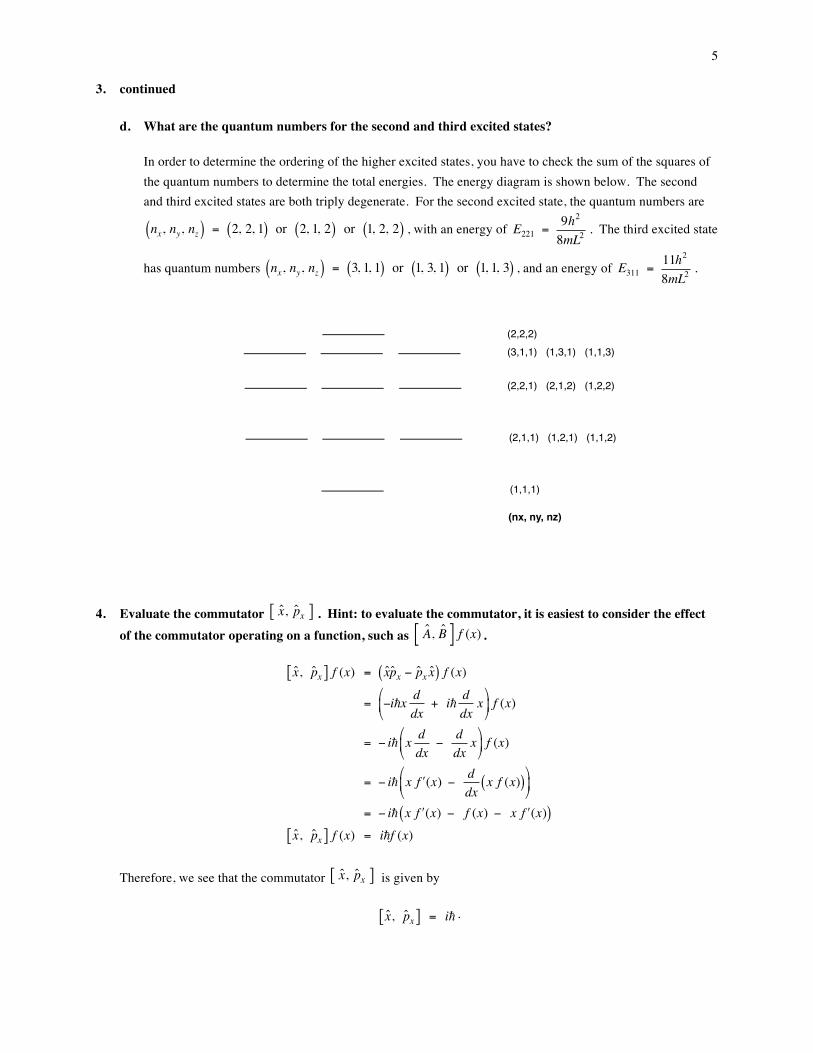
3. continued d. What are the quantum numbers for the second and third excited states?

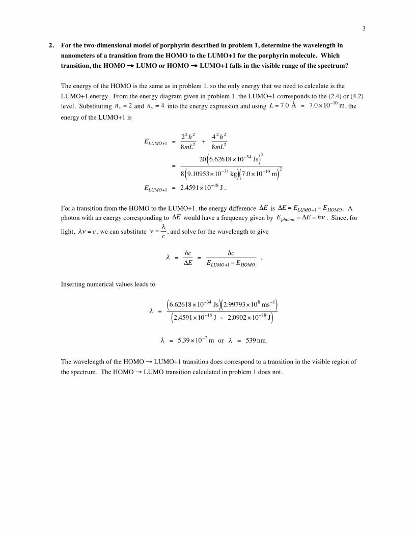
In order to determine the ordering of the higher excited states, you have to check the sum of the squares of the quantum numbers to determine the total energies. The energy diagram is shown below. The second and third excited states are both triply degenerate. For the second excited state, the quantum numbers are

nx, ny, nz( )  =   2, 2, 1( )  or    2, 1, 2( )   or    1, 2, 2( ) , with an energy of E221  =   9h2

8mL2 . The third excited state

has quantum numbers nx, ny, nz( )  =   3, 1, 1( )  or    1, 3, 1( )   or    1, 1, 3( ) , and an energy of E311  =   11h2

8mL2 .

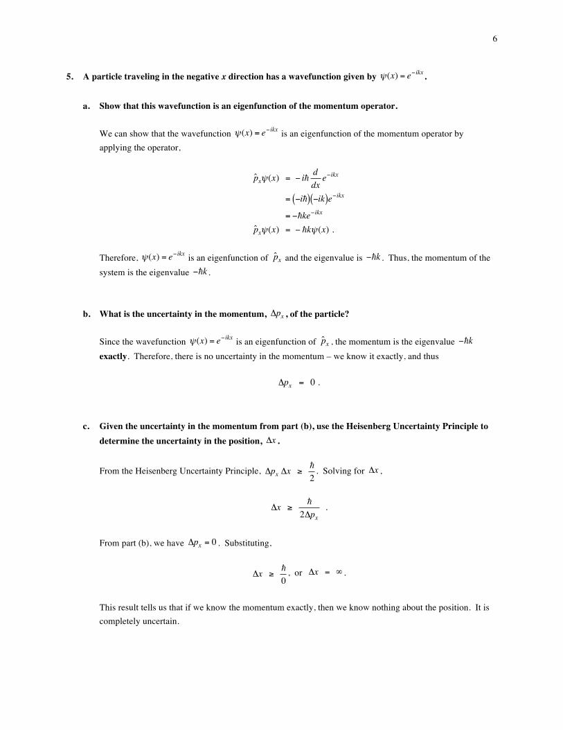
4. Evaluate the commutator

€

ˆ x , ˆ p x[ ] . Hint: to evaluate the commutator, it is easiest to consider the effect of the commutator operating on a function, such as

€

ˆ A , ˆ B [ ] f (x) .

€

ˆ x , ˆ p x[ ] f (x) = ˆ x ̂ p x − ˆ p x ˆ x ( ) f (x)

= −i!x ddx

+ i! ddx

x#

$ %

&

' ( f (x)

= − i! x ddx

− ddx

x#

$ %

&

' ( f (x)

= − i! x ) f (x) − ddx

x f (x)( )#

$ %

&

' (

= − i! x ) f (x) − f (x) − x ) f (x)( )ˆ x , ˆ p x[ ] f (x) = i!f (x)

Therefore, we see that the commutator

€

ˆ x , ˆ p x[ ] is given by

€

ˆ x , ˆ p x[ ] = i! .

(nx, ny, nz)

(2,1,1) (1,2,1) (1,1,2)

(1,1,1)

(2,2,1) (2,1,2) (1,2,2)

(3,1,1) (1,3,1) (1,1,3)

(2,2,2)

6

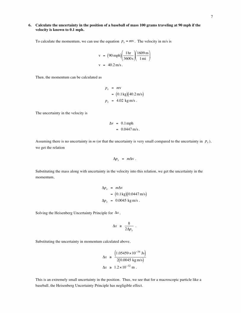
5. A particle traveling in the negative x direction has a wavefunction given by

€

ψ(x) = e−ikx .

a. Show that this wavefunction is an eigenfunction of the momentum operator.

We can show that the wavefunction

€

ψ(x) = e−ikx is an eigenfunction of the momentum operator by applying the operator,

€

ˆ p xψ(x) = − i! ddx

e−ikx

= −i!( ) −ik( )e−ikx

= −!ke−ikx

ˆ p xψ(x) = − !kψ (x) .

Therefore,

€

ψ(x) = e−ikx is an eigenfunction of

€

ˆ p x and the eigenvalue is

€

−!k . Thus, the momentum of the system is the eigenvalue

€

−!k .

b. What is the uncertainty in the momentum,

€

Δpx , of the particle? Since the wavefunction

€

ψ(x) = e−ikx is an eigenfunction of

€

ˆ p x , the momentum is the eigenvalue

€

−!k exactly. Therefore, there is no uncertainty in the momentum – we know it exactly, and thus

€

Δpx = 0 .

c. Given the uncertainty in the momentum from part (b), use the Heisenberg Uncertainty Principle to determine the uncertainty in the position,

€

Δx .

From the Heisenberg Uncertainty Principle,

€

Δpx Δx ≥ !2

. Solving for

€

Δx ,

€

Δx ≥ !2Δpx

.

From part (b), we have

€

Δpx = 0 . Substituting,

€

Δx ≥ !0

, or

€

Δx = ∞ .

This result tells us that if we know the momentum exactly, then we know nothing about the position. It is completely uncertain.

7

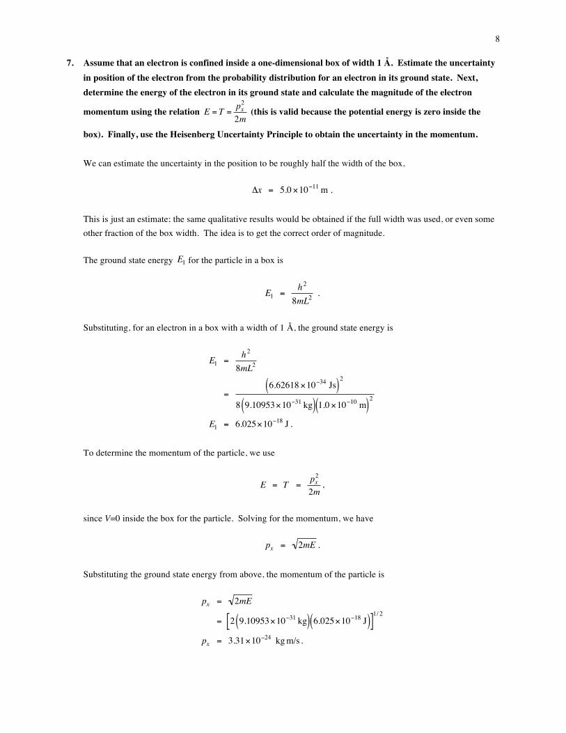
6. Calculate the uncertainty in the position of a baseball of mass 100 grams traveling at 90 mph if the velocity is known to 0.1 mph. To calculate the momentum, we can use the equation

€

px = mv . The velocity in m/s is

€

v = 90 mph( ) 1hr3600s"

# $

%

& '

1609 m1mi

"

# $

%

& '

v = 40.2 m/s .

Then, the momentum can be calculated as

€

px = mv= 0.1kg( ) 40.2 m/s( )

px = 4.02 kg m/s .

The uncertainty in the velocity is

€

Δv = 0.1mph= 0.0447 m/s .

Assuming there is no uncertainty in m (or that the uncertainty is very small compared to the uncertainty in

€

px ), we get the relation

€

Δpx = mΔv . Substituting the mass along with uncertainty in the velocity into this relation, we get the uncertainty in the momentum,

€

Δpx = mΔv= 0.1kg( ) 0.0447 m/s( )

Δpx = 0.0045 kg m/s .

Solving the Heisenberg Uncertainty Principle for

€

Δx ,

€

Δx ≥ !2Δpx

.

Substituting the uncertainty in momentum calculated above,

€

Δx ≥ 1.05459×10−34 Js( )2 0.0045 kg m/s( )

Δx ≥ 1.2×10−32 m .

This is an extremely small uncertainty in the position. Thus, we see that for a macroscopic particle like a baseball, the Heisenberg Uncertainty Principle has negligible effect.

8

7. Assume that an electron is confined inside a one-dimensional box of width 1 Å. Estimate the uncertainty in position of the electron from the probability distribution for an electron in its ground state. Next, determine the energy of the electron in its ground state and calculate the magnitude of the electron

momentum using the relation E = T = px2

2m (this is valid because the potential energy is zero inside the

box). Finally, use the Heisenberg Uncertainty Principle to obtain the uncertainty in the momentum. We can estimate the uncertainty in the position to be roughly half the width of the box,

€

Δx = 5.0×10−11 m . This is just an estimate; the same qualitative results would be obtained if the full width was used, or even some other fraction of the box width. The idea is to get the correct order of magnitude. The ground state energy

€

E1 for the particle in a box is

€

E1 = h2

8mL2 .

Substituting, for an electron in a box with a width of 1 Å, the ground state energy is

€

E1 = h2

8mL2

= 6.62618×10−34 Js( )2

8 9.10953×10−31 kg( ) 1.0×10−10 m( )2

E1 = 6.025×10−18 J .

To determine the momentum of the particle, we use

€

E = T = px2

2m,

since V=0 inside the box for the particle. Solving for the momentum, we have

€

px = 2mE .

Substituting the ground state energy from above, the momentum of the particle is

€

px = 2mE

= 2 9.10953×10−31 kg( ) 6.025×10−18 J( )[ ]1/ 2

px = 3.31×10−24 kg m/s .

9

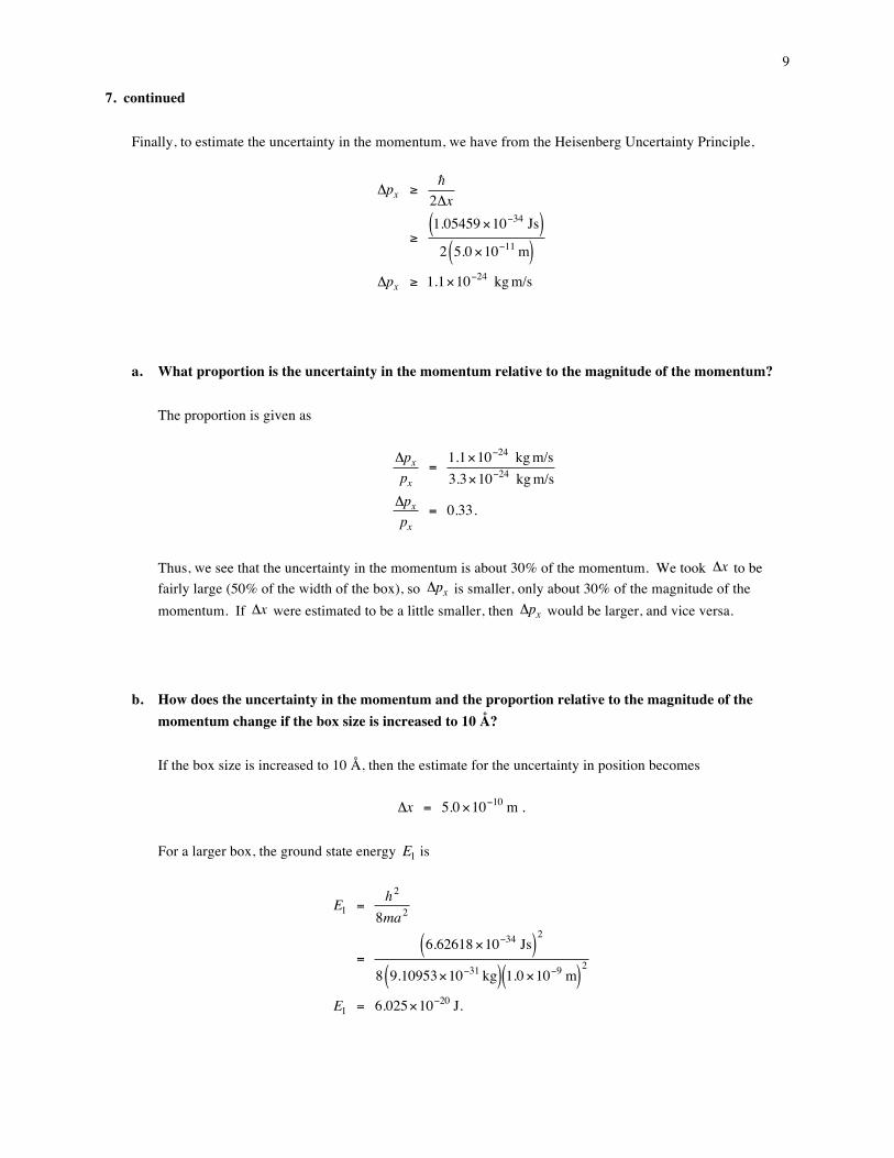
7. continued Finally, to estimate the uncertainty in the momentum, we have from the Heisenberg Uncertainty Principle,

€

Δpx ≥ !2Δx

≥ 1.05459×10−34 Js( )2 5.0×10−11 m( )

Δpx ≥ 1.1×10−24 kg m/s

a. What proportion is the uncertainty in the momentum relative to the magnitude of the momentum? The proportion is given as

€

Δpxpx

= 1.1×10−24 kg m/s3.3×10−24 kg m/s

Δpxpx

= 0.33.

Thus, we see that the uncertainty in the momentum is about 30% of the momentum. We took

€

Δx to be fairly large (50% of the width of the box), so

€

Δpx is smaller, only about 30% of the magnitude of the momentum. If

€

Δx were estimated to be a little smaller, then

€

Δpx would be larger, and vice versa. b. How does the uncertainty in the momentum and the proportion relative to the magnitude of the

momentum change if the box size is increased to 10 Å? If the box size is increased to 10 Å, then the estimate for the uncertainty in position becomes

€

Δx = 5.0×10−10 m .

For a larger box, the ground state energy

€

E1 is

€

E1 = h2

8ma2

= 6.62618×10−34 Js( )2

8 9.10953×10−31 kg( ) 1.0×10−9 m( )2

E1 = 6.025×10−20 J.

10

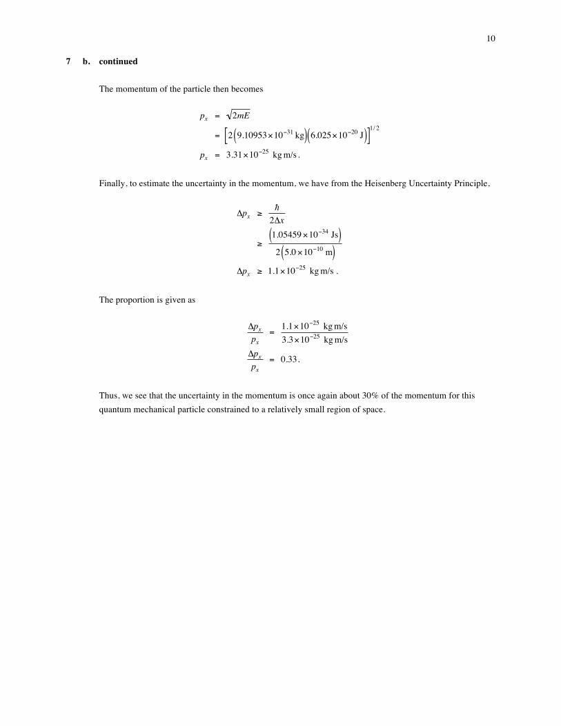
7 b. continued

The momentum of the particle then becomes

€

px = 2mE

= 2 9.10953×10−31 kg( ) 6.025×10−20 J( )[ ]1/ 2

px = 3.31×10−25 kg m/s .

Finally, to estimate the uncertainty in the momentum, we have from the Heisenberg Uncertainty Principle,

€

Δpx ≥ !2Δx

≥ 1.05459×10−34 Js( )2 5.0×10−10 m( )

Δpx ≥ 1.1×10−25 kg m/s .

The proportion is given as

€

Δpxpx

= 1.1×10−25 kg m/s3.3×10−25 kg m/s

Δpxpx

= 0.33.

Thus, we see that the uncertainty in the momentum is once again about 30% of the momentum for this quantum mechanical particle constrained to a relatively small region of space.

11

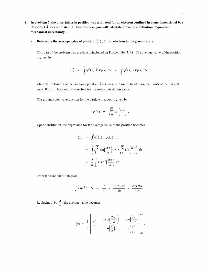
8. In problem 7, the uncertainty in position was estimated for an electron confined in a one-dimensional box of width 1 Å was estimated. In this problem, you will calculate it from the definition of quantum mechanical uncertainty.

a. Determine the average value of position, x , for an electron in the ground state.

This part of the problem was previously included on Problem Set 3, #8. The average value of the position is given by

x =    ψ1*(x)   x̂  ψ1(x) dx

0

a

∫    =     ψ1*(x) x ψ1(x)  dx   

0

  a

∫ ,

where the definition of the position operator,

€

ˆ x = x , has been used. In addition, the limits of the integral are x=0 to x=a because the wavefunction vanishes outside this range. The ground state wavefunction for the particle in a box is given by

ψ1(x)    =     2a sin π x

a⎛

⎝⎜

⎞

⎠⎟  .

Upon substitution, the expression for the average value of the position becomes

x    =     ψ1*(x) x ψ1(x)  dx

0

  a

∫

=     2a sin π x

a⎛

⎝⎜

⎞

⎠⎟ ⋅ x ⋅ 2

a sin π x

a⎛

⎝⎜

⎞

⎠⎟ dx

0

  a

∫

=    2a  x  sin2 π x

a⎛

⎝⎜

⎞

⎠⎟  dx

0

  a

∫ .

From the handout of integrals,

xsin2 bx dx    =    x2

4  ∫ −   xsin2bx

4b   −   cos2bx

8b2 .

Replacing b by πa

, the average value becomes

x = 2a

x2

4 −

xsin 2π xa

⎛

⎝⎜

⎞

⎠⎟

4 πa⎛

⎝⎜

⎞

⎠⎟

− cos 2π x

a⎛

⎝⎜

⎞

⎠⎟

8 πa⎛

⎝⎜

⎞

⎠⎟

2

⎡

⎣

⎢⎢⎢⎢

⎤

⎦

⎥⎥⎥⎥

0

a

.

12

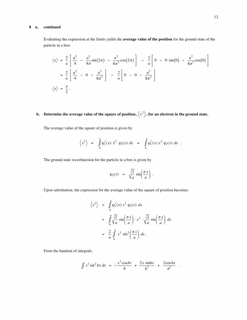
8 a. continued Evaluating the expression at the limits yields the average value of the position for the ground state of the particle in a box:

x = 2a

 a2

4   −   a

2

4πsin 2π( )   −   a

2

8π 2 cos 2π( ) ⎡

⎣⎢

⎤

⎦⎥    −    2

a   0   −   0 ⋅sin 0( )   −    a

2

8π 2 cos 0( ) ⎡

⎣⎢

⎤

⎦⎥

= 2a

 a2

4   −   0   −   a

2

8π 2  ⎡

⎣⎢

⎤

⎦⎥    −    2

a   0   −   0   −   a

2

8π 2  ⎡

⎣⎢

⎤

⎦⎥

x = a2

.

b. Determine the average value of the square of position, x2 , for an electron in the ground state.

The average value of the square of position is given by

x2 =    ψ1*(x)   x̂2  ψ1(x) dx

0

a

∫    =     ψ1*(x) x2 ψ1(x)  dx   

0

  a

∫ .

The ground state wavefunction for the particle in a box is given by

ψ1(x)    =     2a sin π x

a⎛

⎝⎜

⎞

⎠⎟  .

Upon substitution, the expression for the average value of the square of position becomes

x2    =     ψ1*(x) x2 ψ1(x)  dx

0

  a

∫

=     2a sin π x

a⎛

⎝⎜

⎞

⎠⎟ ⋅ x2 ⋅ 2

a sin π x

a⎛

⎝⎜

⎞

⎠⎟ dx

0

  a

∫

=    2a   x2  sin2 π x

a⎛

⎝⎜

⎞

⎠⎟  dx

0

  a

∫ .

From the handout of integrals,

x2 sin2 bx dx∫   =   − x2 cosbxb

 +   2x  sinbxb2   +   2cosbx

b3    .

13

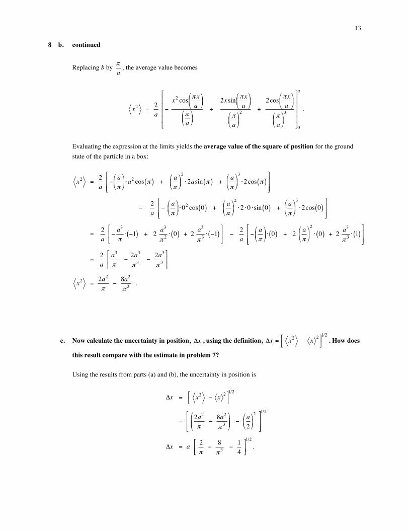
8 b. continued

Replacing b by πa

, the average value becomes

x2 = 2a

− x2 cos π x

a⎛

⎝⎜

⎞

⎠⎟

πa⎛

⎝⎜

⎞

⎠⎟

 +  2xsin π x

a⎛

⎝⎜

⎞

⎠⎟

πa⎛

⎝⎜

⎞

⎠⎟

2  + 2cos π x

a⎛

⎝⎜

⎞

⎠⎟

πa⎛

⎝⎜

⎞

⎠⎟

3

⎡

⎣

⎢⎢⎢⎢

⎤

⎦

⎥⎥⎥⎥

0

a

.

Evaluating the expression at the limits yields the average value of the square of position for the ground state of the particle in a box:

x2 = 2a

−aπ

⎛

⎝⎜

⎞

⎠⎟⋅a2 cos π( )  +  a

π

⎛

⎝⎜

⎞

⎠⎟

2

⋅2asin π( )  + aπ

⎛

⎝⎜

⎞

⎠⎟

3

⋅2cos π( )⎡

⎣⎢⎢

⎤

⎦⎥⎥

                            −    2a

−  aπ

⎛

⎝⎜

⎞

⎠⎟⋅02 cos 0( )  +  a

π

⎛

⎝⎜

⎞

⎠⎟

2

⋅2 ⋅0 ⋅sin 0( )  + aπ

⎛

⎝⎜

⎞

⎠⎟

3

⋅2cos 0( )⎡

⎣⎢⎢

⎤

⎦⎥⎥

=   2a

−a3

π⋅ −1( )  +  2  a

3

π 2 ⋅ 0( )  + 2  a3

π 3 ⋅ −1( )⎡

⎣⎢

⎤

⎦⎥    −   2

a −

aπ

⎛

⎝⎜

⎞

⎠⎟⋅ 0( )  +  2  a

π

⎛

⎝⎜

⎞

⎠⎟

2

⋅ 0( )  + 2  a3

π 3 ⋅ 1( )⎡

⎣⎢⎢

⎤

⎦⎥⎥

=   2a

a3

π  − 2a3

π 3   −  2a3

π 3

⎡

⎣⎢

⎤

⎦⎥ 

x2 =  2a2

π  −  8a

2

π 3   .

c. Now calculate the uncertainty in position, Δx , using the definition, Δx  =    x2   −  x 2⎡⎣

⎤⎦1/2

. How does

this result compare with the estimate in problem 7?

Using the results from parts (a) and (b), the uncertainty in position is

Δx    =      x2   −  x 2⎡⎣

⎤⎦1/2

=     2a2

π  −  8a

2

π 3⎛

⎝⎜⎜

⎞

⎠⎟⎟   −  

a2⎛

⎝⎜⎞

⎠⎟2

 ⎡

⎣⎢⎢

⎤

⎦⎥⎥

1/2

Δx    =  a     2π  −   8

π 3   −  1

4 

⎡

⎣⎢⎤

⎦⎥

1/2

.

14

8 c. continued

Substituting in numerical values, we have

Δx    =  a     2π  −   8

π 3   −  1

4 

⎡

⎣⎢⎤

⎦⎥

1/2

=  a   0.673  −  0.258   −  0.250 [ ]1/2

=    a   0.129 [ ]1/2

Δx    = 0.359a .

So the actual uncertainty is about 36% of the width of the box. In problem 7, we used the uncertainty as 50% of the box, so we were not that far off.