Copyright © UNU-WIDER 2006 * Department of Economics, University of Bristol, UK. This study has been prepared within the UNU-WIDER project on the Millennium Development Goals: Assessing and Forecasting Progress, directed by Mark McGillivray. UNU-WIDER acknowledges the financial contributions to the research programme by the governments of Denmark (Royal Ministry of Foreign Affairs), Finland (Ministry for Foreign Affairs), Norway (Royal Ministry of Foreign Affairs), Sweden (Swedish International Development Cooperation Agency—Sida) and the United Kingdom (Department for International Development). ISSN 1810-2611 ISBN 92-9190-857-6 (internet version)

Research Paper No. 2006/79 Childhood Mortality and Economic Growth Sonia Bhalotra* July 2006

Abstract

This paper investigates the extent to which the decline in child mortality over the last three decades can be attributed to economic growth. In doing this, it exploits the considerable variation in growth over this period, across states and over time. The analysis is able to condition upon a number of economic and demographic variables. The estimates are used to produce a crude estimate of the rate of economic growth that would be necessary to achieve the Millennium Development Goal of reducing the under-5 mortality by two-thirds, from its level in 1990, by the year 2015. The main conclusion is that, while growth does have a significant impact on mortality risk, growth alone cannot be relied upon to achieve the goal.

Keywords: childhood mortality, economic growth, MDGs, India

JEL classification: I12, I31, I32, O15

The World Institute for Development Economics Research (WIDER) was established by the United Nations University (UNU) as its first research and training centre and started work in Helsinki, Finland in 1985. The Institute undertakes applied research and policy analysis on structural changes affecting the developing and transitional economies, provides a forum for the advocacy of policies leading to robust, equitable and environmentally sustainable growth, and promotes capacity strengthening and training in the field of economic and social policy making. Work is carried out by staff researchers and visiting scholars in Helsinki and through networks of collaborating scholars and institutions around the world.

www.wider.unu.edu publications@wider.unu.edu

UNU World Institute for Development Economics Research (UNU-WIDER) Katajanokanlaituri 6 B, 00160 Helsinki, Finland Camera-ready typescript prepared by Adam Swallow at UNU-WIDER The views expressed in this publication are those of the author(s). Publication does not imply endorsement by the Institute or the United Nations University, nor by the programme/project sponsors, of any of the views expressed.

Acknowledgements

I am grateful to Arthur van Soest for many helpful comments, and for inviting me to RAND where this paper was written. I have learnt a lot from Wiji Arulampalam in our discussion of related topics. I would like to thank Mark McGillivray for encouraging me to write this paper and Tony Addison for introducing me to UNU-WIDER.

The Tables and Figures appear at the end of the paper.

1

1 Introduction

A set of time-bound targets for human development were agreed by 189 countries at the Millennium Summit held in New York in September 2000, and these are referred to as the Millennium Development Goals (henceforth MDGs). They represent an unprecedented commitment on the part of both rich and poor countries. One of the eight goals is to reduce under-5 mortality by two-thirds by the year 2015, relative to its level in 1990. This requires an annual rate of decline of about 4.3 per cent p.a.1

This paper is motivated to assess the feasibility of meeting this target in India. India offers an appropriate setting for the analysis as it has one in six of the world’s people, one in four of under-5 deaths, and one in three of the world’s poor. The paper first documents trends in under-5 mortality in India over the period from 1970 to 1998. It then reports estimate of a model of under-5 mortality that includes a rich set of demographic and economic variables. The estimated model parameters can be used to predict mortality in the year 2015 only under what are necessarily arbitrary assumptions. In particular, we would have to assume parameter stability, and we would have to assume a rate of change for every predictor variable (regressor). The analysis is therefore focused on the more specific question of the extent to which economic growth is likely to reduce mortality rates. In particular, it uses the estimated growth elasticity in the recent post-reform era to calculate the rate of growth that would be necessary to achieve the MDG target. It compares this required growth rate with the actual growth rate in the post-reform period.

The analysis investigates variation in the growth elasticity across the Indian states, and over time, considering especially whether it was greater or smaller before the onset of economic reform in the early 1980s. Since childhood mortality is most prevalent amongst poor households, I investigate not just the role of mean income (GDP) but also a potential role for the distribution of income (inequality) in affecting mortality. The paper compares the unconditional growth elasticity with the elasticity obtained conditional upon alternative sets of regressors. The estimates are robust to a range of specification tests, including allowance for dynamics, endogeneity and measurement error.

The main results are as follows. The unconditional growth elasticity of under-5 mortality in India is about -0.7, which means that a 10 per cent increase in GDP is associated with a 7 per cent reduction in mortality. Including state fixed effects pushes the elasticity up to -1.0. Once I also control for year effects, it falls to -0.6. This is consistent with the year effects capturing trend improvements in health technology, the effects of which will tend to be projected upon a trended variable like GDP in a model that does not control for time effects.

I find that higher levels of aggregate income are associated with lower poverty and higher public expenditure on health. However, contrary to expectation, these variables

1 Let M1990 be the under-5 mortality rate in 1990 and let M2015 be the target rate to be achieved by 2015. The total reduction over the 25-year period is (2/3) M1990. So per annum, it is 1-(1/3)1/25=0.0429.

2

do not have large well-determined effects on mortality. Including a measure of public health expenditure and measures of rural and urban poverty in the model does not wipe out the effect of GDP. Controlling for poverty makes little difference to the elasticity. Controlling for government health expenditure results in the GDP elasticity falling to -0.51. These results contradicts the finding in an earlier cross-country analysis of developing country data that GDP has no effect on health indicators once poverty and public expenditure are held constant (Anand and Ravallion 1993).

Estimates of state-specific elasticities show that childhood mortality is responsive to the level of aggregate income (GNP) in only 8 of the 15 major states. Estimates on sub-samples up until and after 1981 indicate that growth was less effective in reducing mortality after 1981, which is when we might date the start of the reform process.

Section 2 summarises causes of childhood death in India, with a view to highlighting mechanisms by which GDP may influence death risk. Section 3 describes related research and outlines the contributions of this paper. The data and descriptive statistics are described in sections 4 and 5 respectively. The estimated equation is set out in section 6, which also discusses the choice of estimator and specification issues. Results are presented in section 7, and conclusions in section 8.

2 Why growth?

In thinking about achieving a target reduction, it is useful to consider what the main causes of under-5 mortality in India are. In contrast to the situation in richer countries, where injuries and accidents are the main cause of childhood death, in poorer countries like India, the main causes of childhood death are poor maternal health, under-nutrition and the prevalence of infectious diseases like malaria, diarrhoea and respiratory infections.2 Most childhood deaths in developing countries are avoidable, and occur for want of household resources, public services and information. So, for instance, increases in household (private) income may be used to improve maternal and child nutrition. Increases in public spending may avert deaths by, for example, improving sanitation, so that less infection is bred, or by increasing the prevalence of skilled midwives and of hospital facilities that might take care of delivery complications. There is a considerable role for information in the production of health by both prevention and cure, and it seems that education makes parents more efficient at acquiring and applying relevant knowledge.

As each of household incomes, public spending and education is likely to have a positive association with the level of aggregate income (GDP), the estimated effect of growth on mortality is expected to capture all of these relationships. Being a reduced form type of effect, it will also capture any interactions between these variables. For

2 The main proximate causes of death, as summarized in Black et al. (2003), are diarrhea, pneumonia, measles, malaria, HIV/AIDS, birth asphyxia, preterm delivery, neonatal tetanus and neonatal sepsis. WHO (1992: Table i) estimates that infectious and parasitic diseases (mainly diarrhea, respiratory diseases like pneumonia and tuberculosis) accounted for 71 per cent of all under-5 deaths in the developing world. Vulnerability to disease is a function of maternal health and child nutritional status- these factors do not appear in classifications such as that of the WHO because they are ‘ultimate’ or underlying rather than proximate causes of death.

3

instance, we may expect the extent to which private or public health spending increases health (or survival chances) to depend upon the level of education of the parent. Household and public spending on health may themselves be complementary. For instance, Jalan and Ravallion (2003) find that the favourable effect of piped water (which depends on public spending) on diarrhoea is lower in poorer households (households with less to spend on child health), especially those with less educated mothers. So, in conclusion, growth in aggregate income provides the resources to make the interventions necessary to reduce mortality. The extent to which growth is effective depends, amongst other things, on the political economy. It is therefore an empirical question, and one on which there is limited evidence as yet (see section 3).

Why analyse the effect of aggregate income (GDP) rather than of a more proximate variable like public expenditure? Because the question of how GDP-growth affects welfare is of wide academic and policy interest. Why is this? One reason is that the evidence on the distributional impact of growth leaves room for concern that the poor do not share equally in its benefits. For an instance of the controversy over the effects of growth on poverty, see Wade (2002) and Bhalla (2002), for example, who offer opposing perspectives. Dollar and Kraay (2002) is an influential study of how pro-poor growth has been over the last four decades in a sample of 92 countries. India-specific studies of the impact of growth on poverty are Besley et al. (2005) and Ravallion and Datt (2002). Research on the effects of growth on mortality is more limited but, as discussed in section 3 below, the few available studies provide what appear to be conflicting results. There is therefore a clear niche for further research on this subject. The other reason that people are interested in growth is probably that the growth elasticity is the natural parameter of interest if the question is ‘how much would mortality would decline, on average, if there were no specific intervention to aid this?’ This is because the level of growth is not directly set by policymakers, while the level of public health expenditure typically is. It is important to emphasise that a focus on the role of growth implies no favour for growth as the instrument for mortality reduction. Indeed, this paper concludes that growth cannot be relied upon to reach a level of mortality consistent with the MDG target.3

3 Related research and contributions

Previous research on mortality in demography has focused on the micro-determinants of mortality, and previous research on mortality in economics is relatively limited (for a useful survey, see Wolpin 1997). This section reviews the evidence from previous research on developing countries that analyses the effect of economic growth on childhood mortality (section 3.1) and that assesses the feasibility of the MDG in health (section 3.2). In section 3.3, I delineate the contributions of this paper.

3 A pragmatic reason that the literature often looks at growth effects rather than at the effects of ‘intermediate’ variables like public expenditure is that it is usually easier to find long and consistent regional time series data on GDP.

4

3.1 The impact of economic growth on childhood mortality

Research on the impact of GDP on mortality in developed countries includes Deaton and Paxson (2001, 2004), Ruhm (2000) and van den Berg et al. (2006). I am aware of three previous studies that seek to estimate the impact of economic growth on mortality in developing countries, and the rest of this section summarises their findings.

Pritchett and Summers (1996) use cross-country panel data for 58 developing countries observed over the period 1960-85. When panel data are available, time-invariant country-specific unobservables can be removed either by first-differencing the data or by including country fixed effects in the model so that the key parameter is estimated on within-country variation. In practice, several authors have taken not annual but five-year differences, or even one long difference (last period minus first period) with a view to reducing measurement error and smoothing over short-term fluctuations (see Durlauf et al. 2005).4 This is also what Pritchett and Summers do, so that the length of their panel is effectively either five or two years. They explain that a further reason for their preferring five-year differences is that the data on under-5 mortality available in international statistics are only collected at 5-yearly intervals. Their fifth-differenced model yields an elasticity of mortality with respect to growth of –0.15, significant at 5 per cent, after controlling for time effects. This falls to –0.12 when education is included in the model. A higher elasticity, of –0.31, is obtained when differencing is replaced by inclusion of country fixed effects. The elasticity is also larger when a single long-difference is taken. As we shall see, the comparable estimate for India is larger, at -0.59. This is similar to the estimate (between –0.5 and –0.6) presented in Kakwani (1993), who uses cross-country data. Pritchett and Summers survey previous estimates of the effect of growth on under-5 or infant mortality, showing that these estimates tend to cluster around the figure of –0.20 (see Hill and King 1992, Subbarao and Raney 1995, Flegg 1982). They caution that these earlier estimates are not strictly comparable with theirs because they are all partial elasticities, emerging from models that condition on variables like infrastructure or health expenditure that are themselves a function of the level of GDP.

Using data for 36 Asian countries for the year 2000, Tandon (2005) estimates an unconditional elasticity (i.e. controlling for neither time not country effects) of –0.7. This is similar to the unconditional elasticity I obtain for India, although Tandon’s elasticity relies on between-country variation, whereas mine relies upon variations across state and time. Tandon does not exploit the panel aspect of his data, and he does not investigate sensitivity of the GDP elasticity to any controls.

The third available study uses Indian data (World Bank 2004).5 Indeed, it uses mortality statistics obtained from the same micro-data source as that used in this paper (see section 3). Probit estimates displayed in the World Bank study indicate the counter-intuitive result that both household living standards and national GDP have a

4 Differencing the data induces autocorrelation in the error term, to address which a GLS or GMM estimator is appropriate. This issue is typically not discussed or addressed.

5 This World Bank report has subsequently been published by its lead author, Anil Deolalikar, as a book by Oxford University Press.

5

positive effect on infant mortality, significant at the 10 per cent level. This result is for infant (under-1) mortality in the five years preceding 1998/9 whereas the results in this paper are for under-5 mortality in the 30 years preceding this date. The results are therefore not directly comparable. Although I could generate results from my analysis for infant deaths in the same 5-year period as the cited study, its results would still not be comparable to those reported in this paper. First, the World Bank study reports a partial effect, obtained conditional upon public health spending and infrastructure, which are themselves functions of GDP. Second, since the model is estimated on cross-sectional data, the effect of GDP is confounded with other, possibly unobservable influences on mortality that, in a panel data model such as estimated in this paper, are captured by state and year effects. The World Bank (2004) study presents an alternative specification of the model using the more aggregative Sample Registration System data on infant mortality for 14 states and 20 years (1980-99). A panel-data regression run on these data, including state fixed effects, yields a more plausible elasticity of mortality with respect to growth of –0.67 (significant at 5 per cent), after controlling for public health expenditure. However, adding a time trend to the model appears to make the GDP effect insignificant.6

3.2 The feasibility of attaining the MDG for mortality in India

I am aware of two previous attempts to assess whether India will achieve the MDG in health. These are described here. The first is more pessimistic than the second, but they are not comparable because they use different approaches, and make different assumptions.

Tandon (2005) documents the annual rate of change in under-5 mortality between 1990 and 2000 in 36 Asian countries. His data show that India ranks 19 of 36, with an annual rate of decline of less than 3 per cent p.a. This is well below the MDG-driven target of 4.3 per cent p.a. that was indicated in section 1 above. In looking at India’s performance, it is useful to note that Bangladesh has done much better despite having slower economic growth than India over this period. It exhibits a rate of decline of under-5 mortality close to 5 per cent p.a., and ranks 6 in 36. Using his unconditional between-country estimate of a GDP-elasticity of –0.7 estimated on cross-country data for the year 2000 (see section 3.1), Tandon estimates that, for the average Asian country in the sample, a rate of growth of GDP of 6 per cent p.a. would be required to achieve the target reduction in under-5 mortality of 4.3 per cent p.a. He acknowledges that, for countries like India that have had mortality declining at less than 4.3 per cent p.a. so far, required growth needs to be even faster in order to catch up. This result is broadly consistent with that in this paper.

The World Bank (2004) report discussed earlier simulates the rate of infant mortality in 2015 under a set of assumptions concerning the rate at which seven significant and policy-amenable predictors will evolve between 1998/9 (the date at which the survey data are gathered) and 2015. These predictors are years of maternal schooling, per

6 What exactly the addition of a trend does to the GDP elasticity cannot be read off Annex Table II.I in the cited report because, in the specification that includes a trend, there is a further change, namely, that GDP is interacted with public health expenditure. The trend and the interaction term are negative and significant but each of GDP and health expenditure become insignificant.

6

capita government expenditure on health and family welfare, population coverage of each of electricity supply, tetanus toxoid immunization for pregnant women, antenatal care and access to toilets, and village-level access to pucca roads. Using the parameters estimated in a multivariate probit model run on micro-data, to predict the change in mortality that would result from changes in each predictor variable, the study concludes that the infant mortality goal, and hence the under-5 mortality goal is achievable in principle. Since this conclusion depends upon the assumed rates at which the named education, health spending and infrastructure or service variables develop, the study performs two related simulations. It isolates the high mortality (and poor) states of Rajasthan, Uttar Pradesh, Madhya Pradesh, Bihar and Orissa from the other (non-poor) states on the grounds that they account for more than half of all childhood mortality. In the first simulation, it takes the levels of the named predictors in these states up to the national average and then, in the second simulation, it takes them up to the average for the non-poor states. The latter procedure yields a rate of decline in the same ballpark as the original simulation, underlining its potential feasibility. The study is careful to point out that actually achieving the target depends, beyond this quantitative analysis, on the composition of public spending and the effectiveness with which public services are delivered.

3.3 Contributions of this paper

With the exception of Pritchett and Summers (1996), no previous research appears to have been primarily concerned with estimating the extent to which economic growth has contributed to mortality reduction in developing countries. This paper extends the work of Pritchett and Summers in a number of ways, summarized here.

Panel data regressions have, in the current context, the important advantage that, by virtue of allowing inclusion of time effects in the model, they allow identification of the effect of GDP as distinct from the effect of other trended variables like health technology. This advantage of panel data comes with a cost. It requires the assumption that technology trends are common across the regions. This is a strong assumption for the sample of 58 developing countries that Pritchett and Summers use. But for the 15 Indian states for which data are pooled in this study, it is fairly plausible to assume technology diffusion and at least some common shocks.

As described in section 3.1, Pritchett and Summers effectively have five or two observations per country. In contrast, I use annual data for a period as long as 30 years. The time effects in my specification are, accordingly, more flexible, and will more effectively capture episodes such as famines or floods that will tend to both reduce GDP and increase mortality. In a model estimated on fifth-differences, it may be difficult to identify transitory shocks like these which may have lasting effects on mortality rates. It is not uncommon in the broader literature to exclude time effects and so to report inflated effects of GDP on human development outcomes. For instance, Ravallion and Datt (1996) appear not to include time effects in their panel data regressions concerning the effect of GDP on poverty and, in a similar analysis, Besley et al. (2005) do not control for time effects in their state-specific models. Deaton and Paxson (2004), using US and UK data, show that omission of time effects in the model tends to inflate the contribution of GDP to mortality reduction. To summarise, the relatively long time series available for the current study assists identification of the impact of GDP growth on mortality, as distinct from the impact

7

of other time-varying factors, many of which may be unobservable to the analyst. The long time series used in this paper has the further advantage that I am able to investigate lags and leads in GDP, and the effects of shocks as well as levels. These investigations are discussed in more detail in Bhalotra (2006).

This paper is rich in the set of covariates it uses. Like Pritchett and Summers, I report estimates of the growth elasticity conditional upon education. However, I also investigate income distribution effects, and attempt to illuminate the mechanisms by which GDP may affect mortality by conditioning upon poverty and public expenditure. Further variants of the model investigate whether the sectoral (agricultural/non-agricultural) composition of growth matters, and whether relative prices or price inflation matter.

In line with Pritchett and Summers, I investigate instrumenting GDP. They use terms of trade shocks as an instrument, whereas I employ a systems estimator and use lags of GDP to instrument its current level. I also investigate over-identifying restrictions associated with rainfall shocks and education. In contrast to Pritchett and Summers, this study corrects the estimated standard errors for heteroskedasticity, clustering and autocorrelation.

4 Data

The mortality data used in this analysis are derived from the second round of the National Family Health Survey conducted in 1998/9; see IIPS and ORC Macro (2000) for details of the survey and sampling strategy. I select data for the 15 major states of India, which (now) account for more than 95 per cent of the country’s population. Over the chosen period, 1970-98, the sample used in the analysis contains 163,907 children of 50,379 mothers. The survey interviewed ever-married women aged 15-49 at the time of the survey. Every mother reported a complete retrospective history of the incidence and timing of live-births and any child deaths. As births in the sample occurred between 1961 and 1999, these data have (unexploited) potential to shed light on trends in fertility, mortality and related demographic change. Issues of possible sample selection in these data are discussed in Bhalotra (2006).

The focus in this study is on under-5 mortality. So I define an indicator variable for child j in family i that is unity if the child is reported to have died before the age of 60 months and zero otherwise. To allow the full 5-year exposure to mortality risk for all children in the sample, children who have not had 60 months exposure (roughly, children born after 1995) are excluded from the analysis. I have aggregated the micro-data from the NFHS to the state level to produce annual mortality rates. These data are merged with a panel of data on real net state domestic product per capita (abbreviated, if inaccurately, as GDP) and other relevant statistics for the 15 Indian states, over the chosen period. These data were assembled by Ozler et al. (1996) and then extended by Besley and Burgess (2002, 2004), who were kind enough to supply me with their database. The merge is done by state and time, where calendar time in the panel is matched to the year of birth of the child in the micro-data (henceforth t). So for children born in 1980 and exposed to the risk of under-5 death during 1980-85, we have matched information on GDP in 1980. In the estimated model, I regress the

8

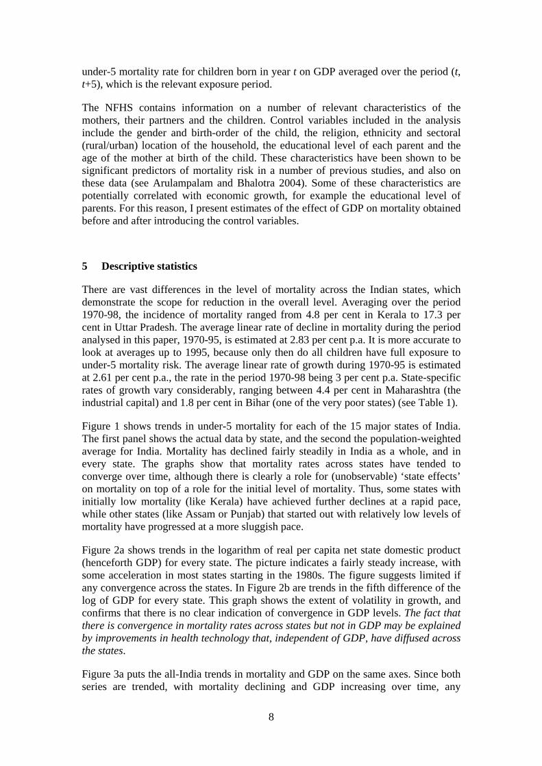
under-5 mortality rate for children born in year t on GDP averaged over the period (t, t+5), which is the relevant exposure period.

The NFHS contains information on a number of relevant characteristics of the mothers, their partners and the children. Control variables included in the analysis include the gender and birth-order of the child, the religion, ethnicity and sectoral (rural/urban) location of the household, the educational level of each parent and the age of the mother at birth of the child. These characteristics have been shown to be significant predictors of mortality risk in a number of previous studies, and also on these data (see Arulampalam and Bhalotra 2004). Some of these characteristics are potentially correlated with economic growth, for example the educational level of parents. For this reason, I present estimates of the effect of GDP on mortality obtained before and after introducing the control variables.

5 Descriptive statistics

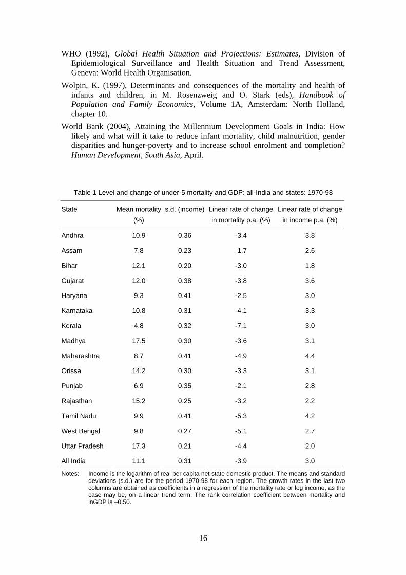
There are vast differences in the level of mortality across the Indian states, which demonstrate the scope for reduction in the overall level. Averaging over the period 1970-98, the incidence of mortality ranged from 4.8 per cent in Kerala to 17.3 per cent in Uttar Pradesh. The average linear rate of decline in mortality during the period analysed in this paper, 1970-95, is estimated at 2.83 per cent p.a. It is more accurate to look at averages up to 1995, because only then do all children have full exposure to under-5 mortality risk. The average linear rate of growth during 1970-95 is estimated at 2.61 per cent p.a., the rate in the period 1970-98 being 3 per cent p.a. State-specific rates of growth vary considerably, ranging between 4.4 per cent in Maharashtra (the industrial capital) and 1.8 per cent in Bihar (one of the very poor states) (see Table 1).

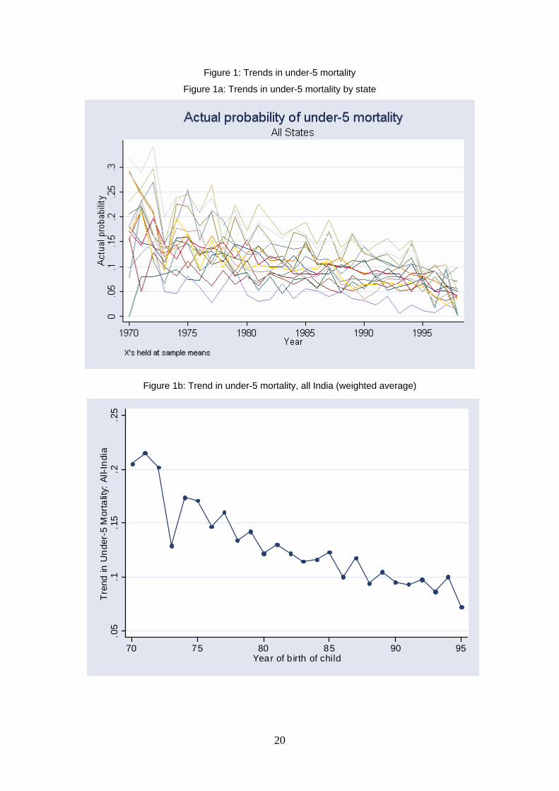
Figure 1 shows trends in under-5 mortality for each of the 15 major states of India. The first panel shows the actual data by state, and the second the population-weighted average for India. Mortality has declined fairly steadily in India as a whole, and in every state. The graphs show that mortality rates across states have tended to converge over time, although there is clearly a role for (unobservable) ‘state effects’ on mortality on top of a role for the initial level of mortality. Thus, some states with initially low mortality (like Kerala) have achieved further declines at a rapid pace, while other states (like Assam or Punjab) that started out with relatively low levels of mortality have progressed at a more sluggish pace.

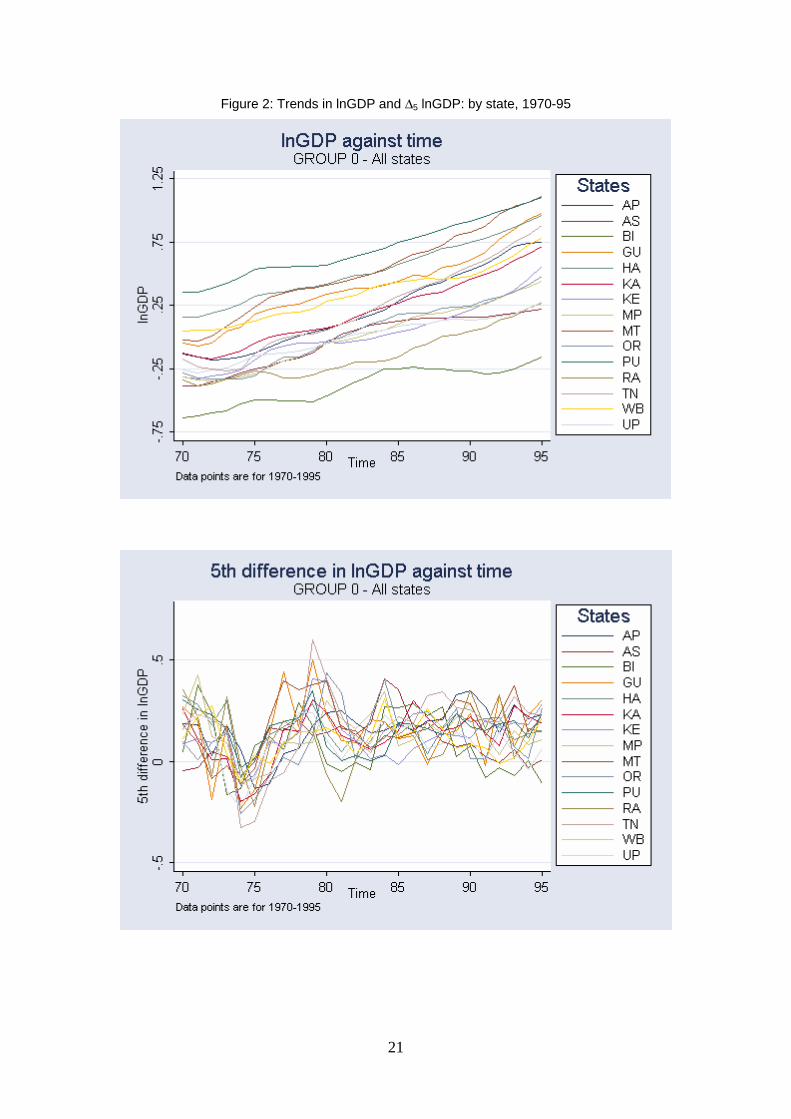
Figure 2a shows trends in the logarithm of real per capita net state domestic product (henceforth GDP) for every state. The picture indicates a fairly steady increase, with some acceleration in most states starting in the 1980s. The figure suggests limited if any convergence across the states. In Figure 2b are trends in the fifth difference of the log of GDP for every state. This graph shows the extent of volatility in growth, and confirms that there is no clear indication of convergence in GDP levels. The fact that there is convergence in mortality rates across states but not in GDP may be explained by improvements in health technology that, independent of GDP, have diffused across the states.

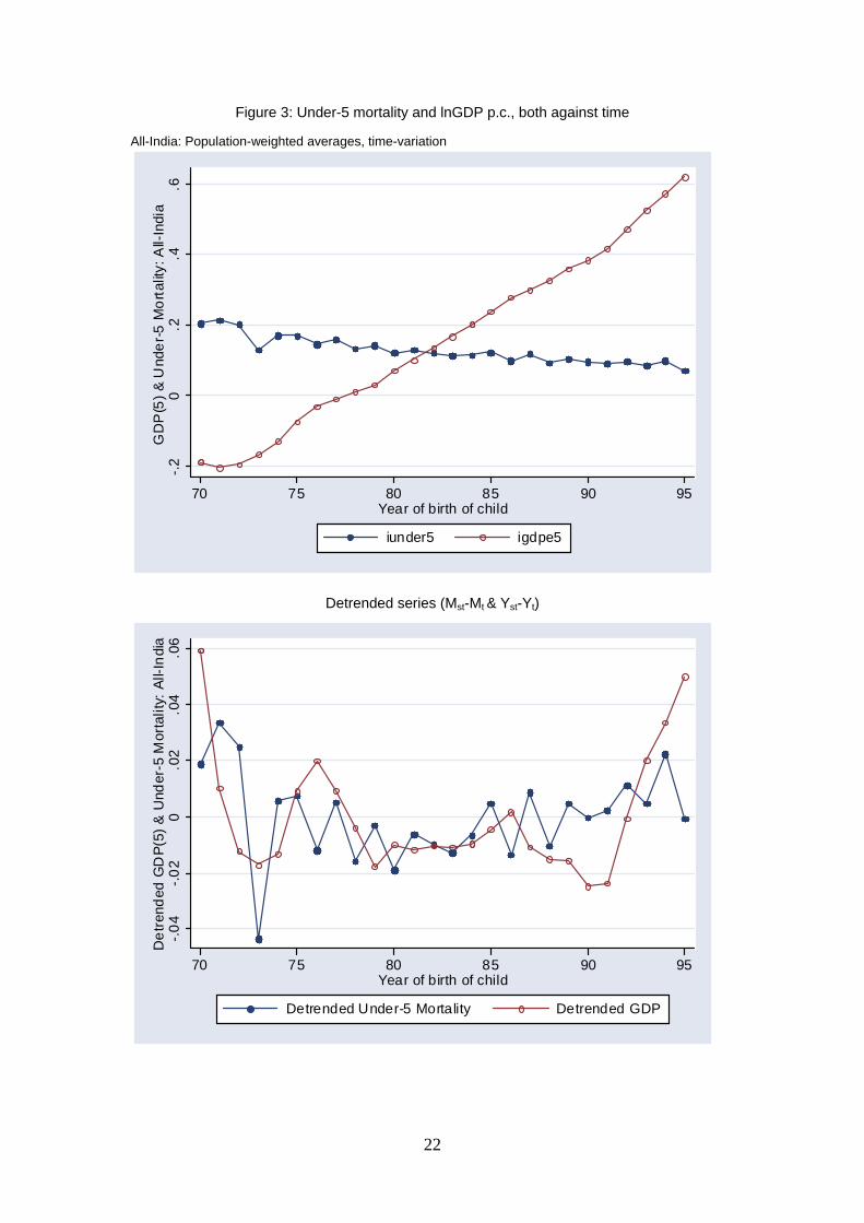
Figure 3a puts the all-India trends in mortality and GDP on the same axes. Since both series are trended, with mortality declining and GDP increasing over time, any

9

correlation between these series will be spurious to the extent that it picks up common trends. For this reason, Figure 3b plots the two time series after de-trending both. This is done by regressing each of mortality and GDP on a set of time dummies and saving the residuals. The plot is of these residuals. This is equivalent to regressing mortality on GDP and a set of time dummies. So what we have in Figure 3b is the relationship that we are really interested in identifying: the relation of growth and mortality after taking out any other trended variables that might otherwise confound the relation. A casual glance at Figure 3b makes it difficult to discern any clear relation. In other words, controlling comprehensively for other trended variables like advances in health technology and services, and for temporal shocks like floods or famines, there is, in the aggregate, no evident relation of growth and mortality.

6 The econometric model

Let M denote the under-5 mortality rate, let Y denote aggregate income (GDP), and let subscripts i, j, s and t denote individual, family, state and year respectively. Then the estimated model may be written as

ln Mst= αs+ αt + β lnYst+ λk ln Zkst + qr ln Xrst + ust (1)

The parameter of interest is β, the elasticity of mortality with respect to GDP.7 The equation includes year and state fixed effects, denoted αt and αs respectively. There are 15 states (s) observed over the course of 25 years (t), 1970-94, giving us a relatively long panel data set. Children born in 1993/4 are exposed to the risk of under-5 death till 1998/9, so the GDP data used extend up until 1998/9. Equation (1) represents the simplest baseline model, but I also investigated dynamics, which previous research in this area appears not to have done. I included the first and second lags of mortality and GDP as additional regressors in the model. As these were insignificant, they were not retained. The equation is estimated by the least squares dummy variables method (or within-groups). Alternative estimators that allow for the endogeneity of GDP are discussed in a companion paper, Bhalotra (2006). I am unable to reject exogeneity of GDP and I show that using instrumental variables does not significantly change the estimated elasticity.

The year fixed effects control comprehensively for aggregate time-variation associated with common improvements in health technology, rainfall variation, terms of trade shocks and so on.State fixed effects control for initial differences in mortality and GDP, and for persistent elements of history, climate, culture (e.g., the status of women) and other institutions (including public service delivery, corruption).

The variables Xr are mostly economic variables and, like GDP, they are defined at the state level. They include inequality, poverty, public spending, relative growth of the agricultural sector, relative prices (rural/urban) and price inflation. The covariates Zk

7 This is what I refer to as the growth elasticity of mortality throughout this paper. As this may be a bit confusing, it is worth clarifying that the relationship is in log-levels, as shown in equation (2). So the level (incidence) of mortality is associated with a level of aggregate income, and economic growth is associated with mortality reduction.

10

are demographic variables that are obtained from the NFHS at the child or family level and then aggregated up to the state level. They include gender, religion, ethnicity, educational level of mother and father, and age of the mother at birth of the index child.

Education and the other demographic variables contribute to controlling for household living standards. The NFHS does not have information on income or consumption at the household level. It has information on housing conditions and ownership of durables which can be used to construct a wealth index (e.g. Filmer and Pritchett 2001). I do not use the wealth information because it pertains to the time of the survey, whereas the births and deaths of children that we are interested in occurred over a long (retrospective) period. To investigate the extent to which education proxies wealth in these data, I regressed the household wealth index on the educational levels of mothers and fathers of children born in the three years before the survey. The R-squared of this regression is 0.37, which I take to mean that parental education is a fairly good proxy for the socio-economic status of the household. While we cannot rule out the possibility that GDP effects in these data are partly proxying omitted household income (see section 2), and we partially investigate this by including the poverty rate in the model, inclusion of the micro-data controls suggests a supply-side (macro) interpretation of the GDP effect. Below, I specifically investigate the role of public expenditure on health.

7 Results

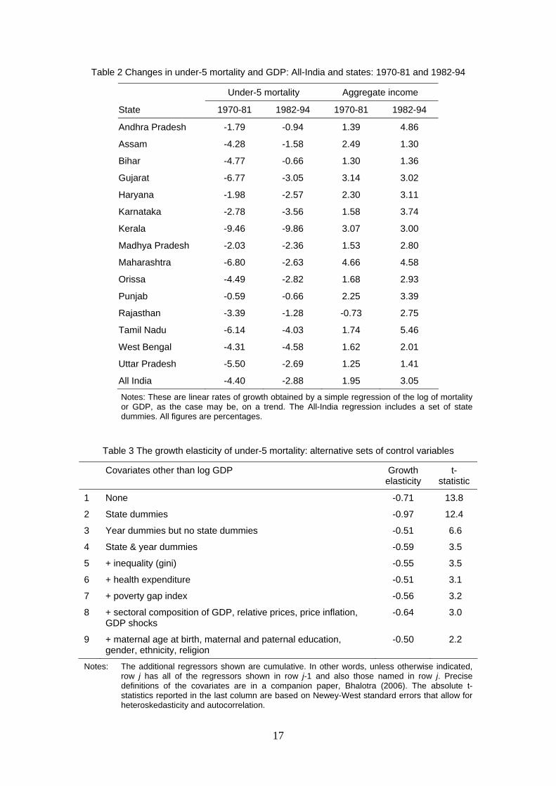
The unconditional elasticity of mortality with respect to aggregate income (GDP) is –0.71, significant at the 1 per cent level.8 Once time and state dummies are included in the model, this falls to –0.59, and remains significant (Table 3). The other rows of Table 3 show that this elasticity is fairly robust to inclusion of other covariates, including public health expenditure and poverty (see section 1).

Precise definitions of the all covariates are in Bhalotra (2006). Here, I summarise the main findings. The state and time dummies are each jointly significant at the 1 per cent level. Conditional on state and time effects, within and between sector inequality, poverty, relative prices (agriculture relative to industry) and inflation are all insignificant. The sectoral composition of GDP is significant. In particular, agricultural growth has a greater mortality-reducing effect than non-agricultural growth. So, at a given level of total GDP, the relative growth rate of the agricultural sector takes a significantly negative coefficient in the mortality equation. In contrast, analyses of the effect of sectoral shifts in GDP on poverty in India find that the greater impact has flowed from non-agricultural growth (see Besley et al. 2005, Ravallion and Datt 2002). Public expenditures on health and family welfare have a significant mortality-reducing effect only at high levels of expenditure. A disaggregate analysis, discussed in more detail in Bhalotra (2006), shows that this effect is significant only in four of the fifteen states, these being Uttar Pradesh, West Bengal, Tamil Nadu and Maharashtra. The only significant compositional effects in the model are secondary-

8 This happens to be almost exactly the same as the unconditional elasticity reported for the UK and the USA in Deaton and Paxson (2004).

11

level education amongst fathers, which reduces child mortality, and belonging to a Scheduled Tribe, which increases mortality.

7.1 Differences in the growth elasticity across the states

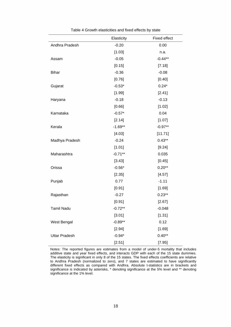
I allow the coefficient on GDP to be state-specific by interacting GDP with state dummies. I find that it is significant in only 8 of the 15 states (see Table 4). In these eight states, the elasticity varies between -0.5 and -0.9, with the exception of Kerala, where the elasticity is a remarkable -1.7.Comparing state GDP effects with state fixed effects, we find that the states that were relatively ineffective in translating growth into lower mortality (i.e. states with a small absolute elasticity) were not those with an inherently high mortality risk (i.e. states with large fixed effects).9 This is encouraging for policy because it suggests that the states in which growth does not significantly reduce mortality can more easily make their growth ‘pro-poor’ (i.e. mortality-reducing) than would be the case if their observed inefficacy were tied to the sorts of persistent historical or institutional factors that state fixed effects tend to capture.

7.2 Was the growth elasticity larger in the post-reform era?

The average growth rate of GDP per capita was barely 1 per cent p.a. in the 1960s and 1970s but, since the early-1980s and especially since about 1993, it has been distinctly higher, averaging 4.8 per cent p.a. between 1993/4 and 1999/00. The upturn in the growth rate coincided with the onset of economic liberalization in India. A gradual process of reform was set in motion in the early to mid-1980s and this accelerated in the 1990s. Whether the reforms caused higher growth, and how, is debatable (see Virmani 2004, Clark and Wolcott 2002, DeLong 2002, Bhalotra 1998) and, in any case, is not the subject of this paper. However, it is interesting to investigate whether the additional growth and the structural change associated with reform altered the growth-elasticity of mortality. For a review of concerns about the impact of structural adjustment on mortality, see Hill and Pebley (1989). Their discussion underlines that the effect can go either way, making this an important question to investigate empirically.

To do this, I split the sample at 1981. A break-point in 1980/1 or 1981/2 is indicated by the analysis in Virmani (2004), who tests for structural breaks in GDP growth in India over the period 1950-2002. Possibly relevant is that the Congress party returned to power in 1980/1, initiating a new approach to economic management in view of growing awareness of the growth-inhibiting constraints of its earlier regime. Table 2 summarises rates of growth of GDP and rates of decline in mortality for the two periods created by a break in 1981. It is clear that, even as the GDP accelerated, mortality decelerated.

Refer to Table 5, where row 1 reports the benchmark estimate of -0.60 from row 4 in Table 3. Rows 2 and 3 show the ‘pre-reform’ and ‘post-reform’ elasticities to be -0.82 and -0.44 respectively, and I am able to reject the null that these are equal at the

9 A similar result is reported in World Bank (2004).

12

10 per cent significance level.10 This result suggests that the Indian reforms were anti-poor (childhood mortality is concentrated amongst the poor: see Victora et al. 2003, for example). In fact, since the mortality rate is bounded, we may expect the elasticity to decrease as the level of mortality decreases even in the absence of any structural change. This is especially the case since, as the incidence of under-5 mortality declines, the fraction of neonatal deaths in all under-5 deaths tends to rise, and neonatal deaths are less closely tied to fluctuations in GDP. All that can be safely concluded is that the post-81 period was not associated with growth becoming evidently more pro-poor than before.

7.3 Simulation to the MDG target

As explained in section 1, given that the MDG for 2015 is benchmarked to the level of mortality in 1990, the annual rate of decline in mortality needs to be 4.3 per cent p.a. over this 25 year period. I estimate the average linear rate of decline of under-5 mortality per annum in India between 1970-95 to have been 2.83 per cent p.a.,11 which implies that, 1995 onwards, a rate of decline faster than 4.3 per cent p.a. will be necessary. We can re-calculate the rate of decline that will be required, benchmarking to a more recent year than 1990. The under-5 mortality rate in 1998 was 9.5 per cent and the target for 2015 is 3.2 per cent (see World Bank 2004: 2). Over the 17-year period between, mortality needs to decline at 6.2 per cent p.a. in order for the target to be met. If mortality were to decline at 2.83 per cent p.a. between 1998 and 2015, the level in 2015 would be 5.83 per cent, which exceeds the target by 2.63 percentage points. These are simple extrapolations, which assume that the predictors of mortality (including GDP) evolve at a constant rate, and that the parameters of the mortality equation are constant over long periods of time. Table 1 shows that GDP-growth rates have varied over time and the previous section shows that the growth-elasticity of mortality has not remained constant over time. The extrapolation exercise is therefore only illustrative.

The more specific question we posed at the start of this paper was: If we were to rely upon GDP growth alone, how far would we be from the MDG target? As mentioned above, the rate of decline of mortality that is necessary between 1998 and 2015 is 6.2 per cent p.a. Using the estimated elasticity of mortality with respect to GDP for the period 1981-94 of –0.44 (Table 5, row 3), we can see that this rate of decline will flow from a rate of GDP growth of 14.1 per cent p.a. Actual GDP growth in the period 1981-94 was 3.1 per cent p.a., and the required growth rate is too high to be feasible. Another way of presenting these data is to say that, if GDP were to continue to grow at 3.1 per cent p.a., then growth alone would generate an annual rate of decline of

10 The regression for 1982-94, like the regression for the full period, 1970-94, allows every child in the sample full exposure to the risk of under-5 mortality, and the GDP variable corresponding for births in 1994 is the average of GDP over 1994-99. To similarly allow for full exposure for every child in the period 1970-81, I re-estimate this model on data for births in 1970-77, with death rates for births in 1977 being modeled as a function of GDP averaged over 1977-81. The pre-reform elasticity is now –1.37 rather than –0.81, and its difference from the post-reform elasticity of –0.44 is significant at the 5 per cent level.

11 I have confirmed that this rate of change is the same for all-India as it for the aggregate of the 15 major Indian states used in this paper (and listed in Table 1).

13

mortality of 1.36 per cent p.a., other things equal. This would result in an under-5 mortality rate of 7.52 per cent in 2015, which is 4.32 percentage points above the target level.

8 Conclusions

Growth does help reduce mortality. The average effect in India is fairly large and quite robust. Yet, growth alone will not deliver mortality reduction at the rate necessary to reach the MDG target. Appropriate policy responses need to recognize that (a) The effectiveness of growth varies across regions, indicating the importance of both the nature of growth and the way in which it is used, and (b) A given level of growth is consistent with different rates of mortality reduction, indicating the importance of other factors that are unrelated to growth. Here is a list of some of the specific findings of this study that are likely to be useful to policy design.

i) Policies that increase the relative growth rate of the agricultural sector will contribute to reducing mortality. After the mid-1970s, agricultural income has grown much more slowly than non-agricultural income in India (e.g. Besley et al. 2005). The analysis in this paper suggests that this has constrained reductions in mortality.

ii) Public health expenditure only has a beneficial effect on mortality at high levels of expenditure. Although this study does not investigate the allocation of public expenditure, it is clear from previous research (e.g. World Bank 2004) that the composition of expenditure and its effective delivery are key to its effectiveness.

iii) Time-varying unobservables that most likely reflect technological change (e.g. medical progress) and improvements over time in health services have contributed significantly to mortality decline, and to the convergence of mortality rates across the Indian states.

iv) Five Indian states account for more than half of all childhood mortality (World Bank 2004). Interventions need to be concentrated in these states. Although this was not specifically investigated in this study, the data show that under-5 death probabilities are higher amongst girls, first-born children and children of scheduled-tribes. Targeting these relatively vulnerable groups will bring down average mortality incidence.

In this study, I interacted GDP with state dummies to obtain state-specific growth elasticities from a panel data model. In work in progress, I replace the state dummies with a vector of variables denoting initial conditions such as female literacy and the initial level of inequality. I will further investigate how the welfare gains from growth may depend upon inequality, media activity and political representation, all of which may be expected to influence the pro-activeness of the state government.

14

References

Anand, S. and M. Ravallion (1993), Human development in poor countries: On the role of private incomes and public services, Journal of Economic Perspectives, 1(3).

Arulampalam, W. and S. Bhalotra (2004), Sibling death clustering in India: genuine scarring vs unobserved heterogeneity. Working Paper 03/552, Department of Economics, University of Bristol. Also forthcoming, Journal of the Royal Statistical Society, Series A.

Besley, T. and R. Burgess (2002), The political economy of government responsiveness: Theory and evidence from India, Quarterly Journal of Economics, 117(4), 1415-52.

Besley, T. and R. Burgess (2004), Can labor regulation hinder economic performance? Evidence from India, Quarterly Journal of Economics, 19(1), 91-134.

Besley, T., R. Burgess and B. Esteve-Volart (2005), Operationalising pro-poor growth: India case study, Mimeograph, Department of Economics, London School of Economics and Political Science.

Bhalla, S. (2002), Imagine There’s No Country: Poverty, Inequality and Growth in the Era of Globalization, Washington DC: Institute for International Economics.

Black, R., S. Morris and J. Bryce (2003), Where and why are 10 million children dying every year? Lancet, 361, 2226-34.

Bhalotra, S. (1998), Changes in utilization and productivity in a deregulating economy, Journal of Development Economics, 57(2), 391-420.

Bhalotra, S. (2006), Health and aggregate wealth: The Indian evidence. Paper presented at LA: RAND, 5 August 2005.

Clark, J. and S. Wolcott (2002), One polity, many countries: Economic growth in India, 1873-2000, in D. Rodrik (ed.), Economic Growth: Analytical Country Narratives, Princeton NJ: Princeton University Press.

Deaton, A. and C. Paxson (2001), Mortality, education, income and inequality among American cohorts, in D. Wise (ed.), Themes in the Economics of Aging, Chicago: University of Chicago Press.

Deaton, A. and C. Paxson (2004), Mortality, income and income inequality over time in Britain and the US, in D. Wise (ed.), Perspectives in the Economics of Aging, Chicago: University of Chicago Press.

DeLong, J. B. (2002), India since Independence: An analytical growth narrative, in D. Rodrik (ed.), Economic Growth: Analytical Country Narratives, Princeton NJ: Princeton University Press.

Dollar, D. and A. Kraay (2002), Growth is good for the poor, Journal of Economic Growth, 7(3), 195-225. Reprinted in A. Shorrocks and R. van der Hoeven (eds) (2004), Growth, Inequality, and Poverty, Oxford: Oxford University Press for UNU-WIDER.

Durlauf, S, P. Johnson and J. Temple (2005), Growth Econometrics, in P. Aghion and S. N. Durlauf (eds) Handbook of Economic Growth Amsterdam: North-Holland, chapter 8 (forthcoming).

15

Filmer, D. and L. Pritchett (2001), Estimating wealth effects without expenditure data – or tears: An application to educational enrollments in states of India, Demography, 38(1), 115-32.

Flegg, A. (1982), Inequality of income, illiteracy and medical care as determinants of infant mortality in underdeveloped countries, Population Studies, 36(3), 441-58.

Jalan, J. and M. Ravallion (2003) Does piped water reduce diarrhoea for children in rural India? Journal of Econometrics, 112(1), 153-73.

Hill, A. and E. King (1992), Women’s education in the Third World: An overview, in E. King and A. Hill (eds), Women’s Education in Developing Countries: Barriers, Benefits and Policy, Baltimore: Johns Hopkins University Press for the World Bank, pp. 1-50.

Hill, K. and A. Pebley (1989), Child mortality in the developing world, Population and Development Review, 15(4), 657-87.

IIPS and ORC Macro (2000), National Family Health Survey (NFHS-2) 1998-9: India. Mumbai: International Institute for Population Sciences.

Kakwani, N. (1993), Performance in living standards: An international comparison, Journal of Development Economics, 41(2): 307-36.

Ozler, B., G. Datt and M. Ravallion (1996), A database on poverty and growth in India, Mimeograph, Washington DC: World Bank.

Pritchett, L. and L. H. Summers (1996), Wealthier is healthier, Journal of Human Resources, 31(4), 841-68.

Ravallion, M. and G. Datt (1996), How important to India’s poor is the sectoral composition of economic growth? World Bank Economic Review, 10(1), 1-25.

Ravallion, M. and G. Datt (2002), Why has economic growth been more pro-poor in some states of India than others? Journal of Development Economics, 68, 381-400.

Rindfuss, R., J. Palmore and L. Bumpass (1982), Selectivity and the analysis of birth intervals from survey data, Asia and Pacific Census Forum, 8(3), 5-16.

Ruhm, C. J. (2000), Are recessions good for your health? Quarterly Journal of Economics, 115(2), 617-50.

Subbarao, K. and L. Raney (1995), Social gains from female education: A cross-national study, Economic Development and Cultural Change, 44(1): 105-28.

Tandon, A. (2005), Attaining Millennium Development Goals in Health: Isn’t Economic Growth Enough? ERD Policy Brief, Series 35, Philippines: Asian Development Bank, March.

van den Berg, G., M. Lindeboom and F. Portrait (2006), Economic conditions early in life and individual mortality, The American Economic Review, 96(1), 290-302.

Victora, C. G., A. Wagstaff, J. A. Schellenberg, D. Gwatkin, M. Claeson and J.-P. Habicht (2003), Applying an equity lens to child health and mortality: more of the same is not enough, Child Survival IV, The Lancet, 362, 19 July.

Virmani, A. (2004), India’s economic growth: From socialist rate of growth to Bharatiya rate of growth, Working Paper 122, New Delhi: Indian Council for Research on International Economic Relations (ICRIER).

Wade, R. (2002), Are global poverty and inequality getting worse? Prospect Magazine, March.

16

WHO (1992), Global Health Situation and Projections: Estimates, Division of Epidemiological Surveillance and Health Situation and Trend Assessment, Geneva: World Health Organisation.

Wolpin, K. (1997), Determinants and consequences of the mortality and health of infants and children, in M. Rosenzweig and O. Stark (eds), Handbook of Population and Family Economics, Volume 1A, Amsterdam: North Holland, chapter 10.

World Bank (2004), Attaining the Millennium Development Goals in India: How likely and what will it take to reduce infant mortality, child malnutrition, gender disparities and hunger-poverty and to increase school enrolment and completion? Human Development, South Asia, April.

Table 1 Level and change of under-5 mortality and GDP: all-India and states: 1970-98

State Mean mortality (%)

s.d. (income) Linear rate of change in mortality p.a. (%)

Linear rate of change in income p.a. (%)

Andhra 10.9 0.36 -3.4 3.8

Assam 7.8 0.23 -1.7 2.6

Bihar 12.1 0.20 -3.0 1.8

Gujarat 12.0 0.38 -3.8 3.6

Haryana 9.3 0.41 -2.5 3.0

Karnataka 10.8 0.31 -4.1 3.3

Kerala 4.8 0.32 -7.1 3.0

Madhya 17.5 0.30 -3.6 3.1

Maharashtra 8.7 0.41 -4.9 4.4

Orissa 14.2 0.30 -3.3 3.1

Punjab 6.9 0.35 -2.1 2.8

Rajasthan 15.2 0.25 -3.2 2.2

Tamil Nadu 9.9 0.41 -5.3 4.2

West Bengal 9.8 0.27 -5.1 2.7

Uttar Pradesh 17.3 0.21 -4.4 2.0

All India 11.1 0.31 -3.9 3.0

Notes: Income is the logarithm of real per capita net state domestic product. The means and standard deviations (s.d.) are for the period 1970-98 for each region. The growth rates in the last two columns are obtained as coefficients in a regression of the mortality rate or log income, as the case may be, on a linear trend term. The rank correlation coefficient between mortality and lnGDP is –0.50.

17

Table 2 Changes in under-5 mortality and GDP: All-India and states: 1970-81 and 1982-94

Under-5 mortality Aggregate income

State 1970-81 1982-94 1970-81 1982-94

Andhra Pradesh -1.79 -0.94 1.39 4.86

Assam -4.28 -1.58 2.49 1.30

Bihar -4.77 -0.66 1.30 1.36

Gujarat -6.77 -3.05 3.14 3.02

Haryana -1.98 -2.57 2.30 3.11

Karnataka -2.78 -3.56 1.58 3.74

Kerala -9.46 -9.86 3.07 3.00

Madhya Pradesh -2.03 -2.36 1.53 2.80

Maharashtra -6.80 -2.63 4.66 4.58

Orissa -4.49 -2.82 1.68 2.93

Punjab -0.59 -0.66 2.25 3.39

Rajasthan -3.39 -1.28 -0.73 2.75

Tamil Nadu -6.14 -4.03 1.74 5.46

West Bengal -4.31 -4.58 1.62 2.01

Uttar Pradesh -5.50 -2.69 1.25 1.41

All India -4.40 -2.88 1.95 3.05

Notes: These are linear rates of growth obtained by a simple regression of the log of mortality or GDP, as the case may be, on a trend. The All-India regression includes a set of state dummies. All figures are percentages.

Table 3 The growth elasticity of under-5 mortality: alternative sets of control variables

Covariates other than log GDP Growth elasticity

t-statistic

1 None -0.71 13.8

2 State dummies -0.97 12.4

3 Year dummies but no state dummies -0.51 6.6

4 State & year dummies -0.59 3.5

5 + inequality (gini) -0.55 3.5

6 + health expenditure -0.51 3.1

7 + poverty gap index -0.56 3.2

8 + sectoral composition of GDP, relative prices, price inflation, GDP shocks

-0.64 3.0

9 + maternal age at birth, maternal and paternal education, gender, ethnicity, religion

-0.50 2.2

Notes: The additional regressors shown are cumulative. In other words, unless otherwise indicated, row j has all of the regressors shown in row j-1 and also those named in row j. Precise definitions of the covariates are in a companion paper, Bhalotra (2006). The absolute t-statistics reported in the last column are based on Newey-West standard errors that allow for heteroskedasticity and autocorrelation.

18

Table 4 Growth elasticities and fixed effects by state

Elasticity Fixed effect

Andhra Pradesh -0.20 0.00

[1.03] n.a.

Assam -0.05 -0.44**

[0.15] [7.18]

Bihar -0.36 -0.08

[0.76] [0.40]

Gujarat -0.53* 0.24*

[1.99] [2.41]

Haryana -0.18 -0.13

[0.66] [1.02]

Karnataka -0.57* 0.04

[2.14] [1.07]

Kerala -1.69** -0.97**

[4.03] [11.71]

Madhya Pradesh -0.24 0.43**

[1.01] [9.24]

Maharashtra -0.71** 0.035

[3.43] [0.45]

Orissa -0.56* 0.20**

[2.35] [4.57]

Punjab 0.77 -1.11

[0.91] [1.69]

Rajasthan -0.27 0.23**

[0.91] [2.67]

Tamil Nadu -0.72** -0.048

[3.01] [1.31]

West Bengal -0.89** 0.12

[2.94] [1.69]

Uttar Pradesh -0.94* 0.40**

[2.51] [7.95]

Notes: The reported figures are estimates from a model of under-5 mortality that includes additive state and year fixed effects, and interacts GDP with each of the 15 state dummies. The elasticity is significant in only 8 of the 15 states. The fixed effects coefficients are relative to Andhra Pradesh (normalized to zero), and 7 states are estimated to have significantly different fixed effects as compared with Andhra. Absolute t-statistics are in brackets and significance is indicated by asterisks, * denoting significance at the 5% level and ** denoting significance at the 1% level.

19

Table 5 Was there a ‘structural break’ in the growth elasticity?

Sample Elasticity t-statistic

1 1970-1994 (entire period) -0.59 3.5

2 1970-1981 (‘pre-reform’) -0.82 2.8

3 1982-1994 (‘post-reform’) -0.44 1.9

Notes: The dependent variable is the log of under-5 mortality, as in Tables 3 and 4. The equations include state and year fixed effects. Standard errors are Newey-West. The elasticities -0.81 and -0.44 are significantly different (F(1,167)=2.7, p>F=0.103).

20

Figure 1: Trends in under-5 mortality

Figure 1a: Trends in under-5 mortality by state

Figure 1b: Trend in under-5 mortality, all India (weighted average)

.05

.1.1

5.2

.25

Tren

d in

Und

er-5

Mor

talit

y: A

ll-In

dia

70 75 80 85 90 95Year of b irth of child

21

Figure 2: Trends in lnGDP and Δ5 lnGDP: by state, 1970-95

22

Figure 3: Under-5 mortality and lnGDP p.c., both against time

All-India: Population-weighted averages, time-variation

-.20

.2.4

.6G

DP

(5) &

Und

er-5

Mor

talit

y: A

ll-In

dia

70 75 80 85 90 95Year of birth of child

iunder5 igdpe5

Detrended series (Mst-Mt & Yst-Yt)

-.04

-.02

0.0

2.0

4.0

6D

etre

nded

GD

P(5)

& U

nder

-5 M

orta

lity:

All-

Indi

a

70 75 80 85 90 95Year of birth of child

Detrended Under-5 Mortality Detrended GDP