Embed Size (px)
Citation preview

“China’s Agricultural Trade: Issues and Prospects”
Edited by Ian Sheldon
Papers presented at an IATRC International Symposium
July 8-9, 2007 Beijing, China
Proceedings Issue
Table of Contents 2
China's Agricultural Trade: Issues and Prospects
TABLE OF CONTENTS
Preface 4 IAN SHELDON Chapter 1: 6 ―China‘s Consumption Driven Growth Path‖ NICHOLAS R. LARDY Chapter 2: 31 ―Are Currency Appreciations Contractionary in China?‖ JIANHUAI SHI Chapter 3: 65 ―A Tale of Two Commodities: China‘s Trade in Corn and Soybeans‖ FRED GALE Chapter 4: 81 ―China‘s Agriculture within the World Trading System‖ GUOQIANG CHENG Chapter 5: 105 ―Integrating China‘s Agricultural Economy into the Global Market: Measuring Distortions in China‘s Agricultural Sector‖ JIKUN HUANG, YU LIU, WILL MARTIN, AND SCOTT ROZELLE Chapter 6: 121 ―Resource Mobility and China‘s Agricultural Trade Policy‖ FUNING ZHONG, JING ZHU, AND ZHENGQIN XIE Chapter 7: 138 ―Long Run Implications of WTO Accession for Agriculture in China‖ KYM ANDERSON, WILL MARTIN, AND ERNESTO VALENZUELA Chapter 8: 159 ―An Assessment of the Economic Effects of COFCO‖ DONALD MACLAREN AND STEVE MCCORRISTON Chapter 9: 183 ―Wage Increases, Labor Market Integration, and the Lewisian Turning Point: Evidence from Migrant Workers‖ FANG CAI, YANG DU, AND CHANGBAO ZHAO Chapter 10: 199 ―Quantitative Evaluation of Agricultural Policy Reforms in China: 1993-2005‖ ANDRZEJ KWIECIŃSKI AND FRANK VON TONGEREN

Table of Contents 3
China's Agricultural Trade: Issues and Prospects
Chapter 11: 222 ―Off-Farm Employment Opportunities and Educational Attainment in Rural China‖ WILLIAM MCGUIRE, BELTON FLEISHER, AND IAN SHELDON Chapter 12: 249 ―Product Quality and the Demand for Food: The Case of Urban China‖ DIANSHENG DONG AND BRIAN GOULD Chapter 13: 280 ―Interactions between Resource Scarcity and Trade Policy: The Potential Effects of Water Scarcity on China‘s Agricultural Economy under the Current TRQ Regime‖ BRYAN LOHMAR AND JAMES HANSEN Chapter 14: 299 ―Genetically Modified Rice, International Trade, and First-Mover Advantage: The Case of India and China‖ GUILLAUME GRUÈRE, SIMON MEVEL, AND ANTOINE BOUËT

Preface 4
China's Agricultural Trade: Issues and Prospects
Preface:
IAN SHELDON
Ohio State University
Preface 5
China's Agricultural Trade: Issues and Prospects
Preface:
China’s Agricultural Trade: Issues and Prospects
In July 2007, at an international symposium organized by the International Agricultural Trade
Research Consortium (IATRC), economists, business professionals and government officials
met in Beijing for two days to discuss the issues and prospects concerning China‘s agricultural
trade. China‘s influence in global agricultural markets has grown substantially and will
continue to grow as the country develops and incomes rise. The IATRC conference in Beijing
provided a forum for experts in the field to share their insight into the current trends in China‘s
agricultural trade, as well as focusing on other key issues that directly or indirectly impact
agricultural trade. As key economic drivers of agricultural production and trade, the
participants discussed China‘s macroeconomic conditions, exchange rates, rural development
and environmental issues, among others. The chapters included in these proceedings provide a
cross-section of many of the major issues and findings from several of the invited and
contributed papers presented at the symposium.
IATRC would like to acknowledge and thank the members of the Organizing Committee,
Colin Carter, Tom Wahl and Lars Brink, for all of their hard work in putting together the
symposium. IATRC also acknowledges and expresses sincere thanks to all of the symposium
sponsors: the Small Farmers Adapting to Global Markets Project, China-Canada Agriculture
Development Program (CCAG); the Department of WTO Affairs, MOFCOM; the Agricultural
Trade Promotion Center, MOA; the Giannini Foundation of Agricultural Economics; the Farm
Foundation; the Ford Foundation; the Economic Research Service (ERS); the IMPACT Center,
Washington State University; and the Ohio Agricultural Research and Development Center,
The Ohio State University. The following organizations are also acknowledged for their
support of the symposium: the China Center for Economic Research (CCER), Peking University;
and the Center for Chinese Agricultural Policy (CCAP), Chinese Academy of Sciences.
Ian Sheldon
IATRC Chair

Lardy Chap.1: China’s Consumption 6
China's Agricultural Trade: Issues and Prospects
Chapter 1:
China’s Consumption Driven Growth Path
NICHOLAS R. LARDY
Peterson Institute for International Economics

Lardy Chap.1: China’s Consumption 7
China's Agricultural Trade: Issues and Prospects
Chapter 1:
China’s Consumption Driven Growth Path*
Introduction
In December 2004 at the annual Central Economic Work Conference, China‘s top political
leadership agreed to fundamentally alter the country‘s growth strategy by rebalancing the
sources of economic growth. In place of investment and export-led development, they
endorsed transitioning to a growth path that relied more on expanding domestic consumption.1
Since then, China‘s top leadership, most notably Premier Wen Jiabao in his speeches to the
annual meetings of the National People‘s Congress in the spring of 2006 and 2007 and at the
Central Economic Work Conference in November- December 2006, has reiterated the goal of
strengthening domestic consumption as a major source of economic growth.2
China‘s decision to rebalance the sources of economic growth is laudable. It increases the
likelihood of China sustaining its strong growth, achieving more rapid job creation, improving
income distribution or at least slowing the pace of rising income inequality, and reducing its
outsized increases in energy consumption of recent years. It also would reduce global economic
imbalances and thus lessen the risk that China would be subject to protectionist pressure,
especially in Europe and the United States.
But at least through the first half of 2007, China‘s economic growth has become even more
imbalanced. Although the growth of investment expenditures has moderated slightly, net
exports of goods and services have soared. China‘s external surplus ballooned to a global
record in 2006 and continued to expand at a breakneck pace in the first half of 2007. Most
importantly, both government and private consumption expenditure as a share of GDP have
* An earlier version of this paper, published as ―China: Rebalancing Economic Growth‖ in The China Balance Sheet in 2007 and Beyond (Washington, D.C.: Center for Strategic and International Studies and Peterson Institute for International Economics, April 2007), is available at: http://www.petersoninstitute.org/publications/papers/lardy0507.pdf. 1 ―Central Economic Work Conference Convenes in Beijing December 3 to 5,‖ People’s Daily, December 6, 2004, 1, available at: http://www.people.com.cn. (accessed July 21, 2006). 2 Wen Jiabao, ―Report on the Work of the Government,‖ People’s Daily, March 14, 2006, http://english.people.com.cn (accessed March 14, 2006). New China News Agency, ―We must concretely grasp eight work items to do well in next year‘s economic work,‖ December 1, 2006 at http://politics.people.com.cn/GB/1024/3907488.html (accessed December 12, 2006). Wen Jiabao, ―Report on the Work of the Government,‖ March 5, 2007.

Lardy Chap.1: China’s Consumption 8
China's Agricultural Trade: Issues and Prospects
continued to fall since 2004. As a consequence, China also is falling short of meeting several of
its key domestic economic objectives.
The Sources of China’s Economic Growth
China has been the fastest growing economy in the world over almost three decades, expanding
at 10% a year in real terms, so real GDP in 2006 was about 13 times the level of 1978, when Deng
Xiaoping launched China on the path of economic reform (National Bureau of Statistics of
China, 2006a, p.24; Xie Fuzhan, 2007). China is now the world‘s fourth largest economy and its
third largest trader and highly likely, within a year, to move up a notch in each category. Given
this stunning long-term success, why would China‘s leadership entertain the idea of shifting to
a new growth paradigm?
In all economies the expansion of output is the sum of the growth of consumption (both
private and government) plus investment, plus net exports of goods and services. Expanding
investment has been an increasingly important driver of China‘s growth. As shown in Figure 1,
investment averaged 36% of GDP in the first decade or so of economic reform, relatively high
by the standard of developing countries generally but not in comparison with China‘s East
Figure 1: Investment as percent of GDP, 1978-2006
20
25
30
35
40
45
78 79 80 81 82 83 84 85 86 87 88 89 90 91 92 93 94 95 96 97 98 99 00 01 02 03 04 05 06
Percent
Source: National Bureau of Statistics of China, China Statistical Yearbook 2006; CEIC

Lardy Chap.1: China’s Consumption 9
China's Agricultural Trade: Issues and Prospects
Asian neighbors when their investment shares were at their highest. But since the beginning of
the 1990s, China‘s average investment rate has been higher and in 1993, and again in 2004-06,
reached 43% of GDP, a level above the experience of China‘s East Asian neighbors in their high
growth periods.3 Rising investment has been fueled by a rise in the national savings rate, which
reached an unprecedented 52% of GDP in 2006.4 Rising investment was particularly important
in 2001-2005, when it contributed just over half of China‘s growth (National Bureau of Statistics
of China, 2006b, p.70), an unusually high share by international standards.
The growth of both household and government consumption (Figures 2 and 3) has been
rapid in absolute terms throughout the reform period, but has lagged the underlying growth of
the economy. As shown in Figure 2, in the 1980s household consumption averaged slightly
more than half of GDP. This share fell to an average of 46% in the 1990s. But after 2000
household consumption as a share of GDP fell sharply—and by 2006 accounted for only 36% of
3 All of the analysis of the expenditure components of GDP, i.e. consumption, investment, and net exports, is based on the revised GDP expenditure data for the years 1978 through 2005 released by the National Bureau of Statistics of China (2006b) in late September 2006. Data for 2006 were released in May 2007. 4 By definition, the national savings rate is equal to investment as a share of GDP plus the current account as a percent of GDP. In China, these were 42.7% and 9.5% of GDP, respectively, in 2006.
Figure 2: Household consumption as percent of GDP, 1978-2006
30
35
40
45
50
55
78 79 80 81 82 83 84 85 86 87 88 89 90 91 92 93 94 95 96 97 98 99 00 01 02 03 04 05 06
Percent
Source: National Bureau of Statistics of China, China Statistical Yearbook 2006; CEIC

Lardy Chap.1: China’s Consumption 10
China's Agricultural Trade: Issues and Prospects
GDP, by far the lowest share of any economy in the world.5 In the United States, household
consumption accounted for 70% of GDP in the same year. In the United Kingdom, the
household consumption share was 60%. In India, it was 61%.
As a result of these trends in household and government consumption, the relative
importance of expanding consumption as a source of growth has diminished substantially,
particularly compared with that of investment. In the first half of the 1980s consumption
growth accounted for almost four-fifths of China‘s economic expansion, whereas in the five-
year period 2001-2005, this share fell by one-half to only two-fifths (National Bureau of Statistics
of China, 2006b, p.70).
5 The declining share of consumption in GDP is due to both a decline in household disposable income as a share of GDP and a decline in consumption as a share of disposable income. Some analysts believe that household consumption, particularly of services, is undercounted by China‘s National Bureau of Statistics and thus the share of household consumption in GDP is biased downwards. If GDP was undercounted by 8% or 12%, and the entire increment was private consumption of services, household consumption would have constituted 42% and 44%, respectively, of GDP in 2005 (Dragoneconomics Research & Advisory, 2007). Even on these alternative assumptions, however, private consumption as a share of GDP would be unusually low by international standards. These adjustments would also lower the investment share of GDP by 3 and 4 percentage points, respectively. The higher consumption and lower investment share of GDP would mean the degree of internal imbalance is less than that reflected in the official data. Note, however, that on these alternative assumptions, China‘s large and growing external imbalance would decline by only a few tenths of a percentage point.
Figure 3: Government consumption as percent of GDP, 1978-2006
10
11
12
13
14
15
16
17
78 79 80 81 82 83 84 85 86 87 88 89 90 91 92 93 94 95 96 97 98 99 00 01 02 03 04 05 06
Percent
Source: National Bureau of Statistics of China, China Statistical Yearbook 2006; CEIC

Lardy Chap.1: China’s Consumption 11
China's Agricultural Trade: Issues and Prospects
In the last two years, the growth of net exports of goods and services has also become, for
the first time in almost a decade, a major source of economic growth. As shown in Figure 4, the
net exports of goods and services in 2005 more than doubled to reach $124 billion and
accounted for one-quarter of the growth of the economy (National Bureau of Statistics of China,
2006b, p.70). In 2006 they expanded further to $209 billion and accounted for about one-fifth of
China‘s growth (State Administration of Foreign Exchange International Balance of Payments
Analysis Small Group, 2007, p.8).
In sum, despite the decision of the Party in 2004 to stimulate domestic consumption
demand, both household and government consumption have continued to fall as a share of
GDP. The government has been more successful in moderating the growth of investment and
thus the contribution of investment to GDP expansion has fallen from the extraordinarily high
levels of 2002-2003. On the other hand net exports of goods and services have soared and their
contribution to economic growth is currently unusually large leading, Premier Wen Jiabao at
the National People‘s Congress in the spring of 2006 to opine that ―we must strive to reduce our
excessively large trade surplus.‖
Figure 4: Net exports of goods and services, 1992-2006
-50
0
50
100
150
200
250
1992 1993 1994 1995 1996 1997 1998 1999 2000 2001 2002 2003 2004 2005 2006
Percent US$ Billion
-4.00
-2.00
0.00
2.00
4.00
6.00
8.00
Percent of GDP (RHS)
Goods and Services Balance (LHS)
Source: National Bureau of Statistics of China, China Statistical Yearbook 2006; International Monetary Fund, International Financial Statistics; CEIC

Lardy Chap.1: China’s Consumption 12
China's Agricultural Trade: Issues and Prospects
Rethinking China’s Growth Strategy
Several factors appear to underlie the December 2004 leadership decision to rebalance the
sources of growth. First, investment-driven growth, or what the Chinese sometimes call
extensive growth, appeared to be leading to less efficient use of resources. By some metrics, as
investment growth accelerated, the efficiency of resource use declined. Multifactor productivity
growth, a critical contributor to economic expansion in all economies, averaged almost 4% per
annum in the first 15 years of economic reform (1978–93) but slowed to only 3% since 1993
(Kuijs and Wang, 2005, p.2). In short, as the investment share of GDP rose, the contribution of
productivity improvements to GDP growth fell. In the words of Martin Wolf (2005), the chief
economics commentator for the Financial Times, the surprising thing about the Chinese economy
in recent years is not, as is so frequently asserted, how fast it is growing but rather, given the
outsized share of output devoted to investment, how slowly it is growing.
The second reason underlying the leadership decision to rebalance the sources of growth is
the desire to increase personal consumption and alleviate, or at least slow, the pace of
increasing income inequality. In 2005, personal consumption in China was 30% less in real
terms than the level that would have been achieved if the household consumption share of GDP
had remained at the 1990 level rather than falling by more than 10 percentage points. India
offers a useful comparison. In 2004 China‘s per capita GDP was two and a half times that of
India. But, because household consumption as a share of GDP was so much lower in China, per
capita consumption exceeded that in India by only two-thirds.6 The ultimate purpose of
economic growth everywhere is improvements in human welfare. By this standard, China is
falling far below potential.
Similarly, it appears that a portion of increasing income inequality in recent years can be
attributed to the highly imbalanced regional pattern of growth. The positive differential in the
pace of growth in coastal provinces compared to the national average has increased along with
the sharply higher pace of growth of foreign trade (particularly exports) that has occurred since
2000.7 Moving away from heavy reliance on export led growth thus is consistent with Hu
6 Calculated on the basis of the Indian Ministry of Statistics and Program Implementation, National Account Statistics, available at: http://mospi.nic.in , IMF, International Financial Statistics; and National Bureau of Statistics of China (2006b, pp. 34, 36, 171). 7 From 1978 through 2000 China‘s trade turnover (imports plus exports) measured in value terms expanded at an average rate of 15 per cent per year. From 2000 through 2006 the pace accelerated to 25 per cent per year.

Lardy Chap.1: China’s Consumption 13
China's Agricultural Trade: Issues and Prospects
Jintao‘s emphasis on, creating a more ―harmonious society,‖ which requires, among other
things, more balanced development between coastal and inland areas.
Third, China‘s extensive pattern of development has generated very modest gains in
employment. Between 1978 and 1993, employment expanded by 2.5% per annum, but between
1993 and 2004, when the investment share of GDP was much higher than in the 1980s,
employment growth slowed to only slightly over 1% (Kuijs and Wang, 2005). The recent more
capital intensive pattern of growth contributed to a slower pace of job creation for the simple
reason that the steel and other investment goods industries employ far fewer workers per unit
of capital than do consumer goods industries, not to mention the even less favorable
comparison with services.
Another reason China‘s leadership wishes to transition to a more consumption-driven
growth path is burgeoning energy consumption and its detrimental effects on the environment.
Investment-driven growth requires the output of machinery and equipment, and the inputs to
produce them, to grow much more rapidly than the output of consumer goods. Rapid growth
of output of investment goods, in turn, increases the demand for energy disproportionately.
China‘s energy elasticity of GDP growth (the number of units of energy required to produce an
additional unit of output) averaged a modest 0.6 in the 1980s and 1990s, leading over time to a
substantial reduction in the amount of energy required to produce each unit of GDP. But this
ratio rose to an average of 1 in 2001-05 (National Bureau of Statistics of China, 2006a, p.147).
Although China continues to achieve energy efficiency gains in the production of virtually all
products, from 2001 through 2005 these gains were no longer sufficient to offset the effect of the
rapid expansion of the most energy intensive sectors of manufacturing, including steel,
chemicals and cement.8
Since two-thirds of China‘s energy comes from coal, the burgeoning demand for energy
generated by capital-intensive growth boosted coal consumption by two-thirds between 2000
and 2005. Coal consumption reached more than 2 billion tons in 2005, almost twice the level of
coal consumption of the United States, even though China‘s economy is only one-sixth the size
of the United States. As a result, China is now the second largest emitter of greenhouse gas and
is home to 16 of the 20 cities with the worst air pollution on the globe. As a result of the massive
8 For example, in 2003 overall efficiency gains were the equivalent of about 30% of the adverse effect on energy efficiency stemming from the structural shift toward the most energy intensive subsectors of the industrial sector (Jin, 2006).

Lardy Chap.1: China’s Consumption 14
China's Agricultural Trade: Issues and Prospects
increase in coal consumption, the State Environmental Protection Agency (SEPA) reported that
rather than cutting sulfur dioxide emissions in 2000–2005 by 10% to 18 million tons as planned,
by 2005 emissions rose to 25.5 million tons, 42% above the goal.9
A fifth factor motivating China‘s leadership to seek a transition to a more consumption-
driven growth pattern is less obvious but still important. Excessive reliance on investment and
net exports to drive growth in recent years threatens to undo some of the progress China has
made over the past six years in developing a commercially oriented banking system. A critical
component of this process has been the injection of almost 4 trillion renminbi (RMB) ($500
billion), mostly from the government, to cover past loan losses and to raise capital adequacy to
meet prudential standards (Ma Guonan, 2006).
Excess investment in some sectors could eventually lead to excess capacity and falling
prices, which could create a new wave of nonperforming loans that would erode the substantial
balance sheet improvements of state-owned banks over the past few years and could push some
city commercial banks, which on average are far weaker, into insolvency. The National
Development and Reform Commission (2006) in its report to the National People‘s Congress
9 Oster, 2006.
Figure 5: Losses of unprofitable industrial enterprises, 1995-2006
0
50
100
150
200
250
1995 1996 1997 1998 1999 2000 2001 2002 2003 2004 2005 2006
RMB bn
Source: National Bureau of Statistics of China, China Statistical Yearbook 2006; CEIC

Lardy Chap.1: China’s Consumption 15
China's Agricultural Trade: Issues and Prospects
acknowledged that ―adverse effects of surplus production capacity in some industries have
begun to emerge. Prices for the products of these industries dropped and inventories grew,
corporate profits shrank and losses mounted, and potential financial risk has increased.‖ This
analysis is supported by the rapid increase in the magnitude of financial losses of unprofitable
industrial enterprises. As shown in Figure 5, after several years of stability, losses have more
than doubled since 2003. Since net profits of all enterprises rose sharply in this period (see
Figure 7) there apparently has been a sharp increase in the dispersion of the profitability of
China‘s industrial firms over the past three years.
The absence of significantly rising non-performing loans in the banking system in the past
few years is not necessarily a sign that all is well, since China has had four consecutive years of
double-digit growth and aggregate corporate profits have been rising. Moreover, based on
China‘s exploding current account surplus in recent years (see Figure 6 and related discussion
below) the RMB appears to be increasingly undervalued, contributing to the growth of profits
in the tradable goods sector, i.e., manufacturing. Distress in the banking system could emerge,
however, either from a slowdown in economic growth over the next few years or from a
significant appreciation of the currency.
A final factor underlining the leadership‘s desire to transition to more consumption-
oriented growth is that excess reliance on a growing trade surplus raises the prospect of a
protectionist backlash in the United States, Europe, and other important markets for Chinese
exports. China‘s central bank was perhaps the first to explicitly acknowledge this factor in its
Report on the Implementation of Monetary Policy Report 2005Q2, in which it candidly stated that
China‘s excessive trade surplus ―will escalate trade frictions‖ (People‘s Bank of China Monetary
Policy Analysis Small Group, 2005, p.28).
In sum, for a variety of reasons China‘s top political leadership and its leading economic
advisory institutions by late 2004 came to the view that sustaining long-term rapid growth
required a significant modification of the underlying growth strategy.
Implications for the Global Economy
China‘s new growth strategy, if realized, would have positive implications not only for China,
but also for the global economy. As shown in Figure 6, China‘s current account surplus has
soared in recent years. In 2006 it reached $249 billion making China, for the first time, the
world‘s largest global current account surplus country. China now is a major contributor to

Lardy Chap.1: China’s Consumption 16
China's Agricultural Trade: Issues and Prospects
global economic imbalances, along with the United States, which has the world‘s largest current
account deficit. China‘s successful transition to a pattern of growth driven more by domestic
consumption demand necessarily entails a reduction of China‘s national saving rate relative to
its investment rate. That, in turn, would reduce China‘s current account surplus. Thus
rebalancing of China‘s economic growth would contribute to a reduction of global economic
imbalances as well.
Promoting Consumption Driven Growth
Promoting domestic demand as a source of economic expansion requires that the growth of
household and/or government consumption increase relative to that of the combined growth of
investment and net exports. Policies to promote consumption fall into three broad categories:
fiscal, exchange rate, and financial. Fiscal policy options include cutting personal taxes,
increasing government consumption expenditures, i.e., government noninvestment outlays, or
introducing a dividend tax on state-owned companies. Appreciation of the RMB would
simultaneously reduce net exports and allow the government greater flexibility in the use of
interest rate policy (Goodfriend and Prasad, 2006). As will be argued below, higher real interest
rates are almost certainly necessary to reduce China‘s excessive rate of investment, which in
Figure 6: Current account balance as percent of GDP, 1994-2006
0
2
4
6
8
10
1994 1995 1996 1997 1998 1999 2000 2001 2002 2003 2004 2005 2006
Percent
Source: National Bureau of Statistics of China, China Statistical Yearbook 2006; State Administration of Foreign Exchange of China Website.

Lardy Chap.1: China’s Consumption 17
China's Agricultural Trade: Issues and Prospects
turn is a prerequisite to a successful transition to a more consumption-driven growth path.
Finally, financial reform could increase interest income received by households, potentially
raising household disposable income and thus consumption.
Fiscal Policy: The most obvious policy choice in economies seeking to stimulate
consumption is to cut personal taxes, thus raising disposable income and personal consumption
expenditures. In addition, governments can increase budgetary expenditures, notably those on
health, education, welfare, and pensions, to add to domestic consumption demand. There is
enormous scope to do so in China, since governments at all levels combined spend only 3% of
GDP on these programs (National Bureau of Statistics of China, 2006b, p.288).10 The low level of
social expenditure is reflected in the very limited share of the population that has health,
unemployment and workers‘ compensation insurance. In 2003, for example, in urban areas only
about one-half of the population was covered by basic health insurance, and in rural areas less
than one-fifth of the population was covered by a cooperative health insurance program
initiated on a trial basis in 2002 (OECD, 2005, p.185). In 2005, only 14% of China‘s workforce
was covered by unemployment insurance, and only 11% were covered by workers‘
compensation (National Bureau of Statistics of China, 2006a, pp. 43, 201). In the same year the
pension scheme covered 131.2 million workers, only 17% of those employed, plus 43.7 million
retirees (National Bureau of Statistics of China, 2006a, pp. 43, 201).
The government has considerable potential to increase its expenditures on healthcare,
unemployment compensation, and pensions without raising taxes on households, which likely
would depress household consumption, offsetting to some degree the increase in government
consumption. The government could simply reduce its own investment expenditures and
reallocate the funds to consumption.11 The government itself directly undertakes about 5% of all
investment, an amount equivalent to a little over 2% of GDP (National Bureau of Statistics of
China, 2006a, p.52). In addition, the government budget provides ―capital transfers,‖ that are
used to finance additional investment expenditures.12 For 2003, the most recent year for which
China‘s National Bureau of Statistics has released the relevant data, these capital transfers were
the equivalent of 8% of all fixed investment (National Bureau of Statistics of China, 2006b, pp.
10 Excluding capital expenditures. 11 This reallocation, of course, would reduce government savings since the latter are defined as current revenues less current, i.e., noninvestment, outlays. 12 Kuijs (2006, p.7) believes these funds are transferred to state-owned enterprises in electric power, water, transport, and other infrastructure sectors.
Lardy Chap.1: China’s Consumption 18
China's Agricultural Trade: Issues and Prospects
88-89). Thus the government‘s direct and indirect investment outlays combined amount to
about 6% of GDP. A reduction in the government‘s direct investment and cutting capital
transfers would free up resources to increase government consumption, i.e., outlays for health,
education, welfare, and pensions. That would contribute significantly to a rebalancing of the
structure of demand, away from investment and toward consumption.
Increased government consumption expenditures would also indirectly contribute to
increasing household consumption as a share of GDP by reducing the household savings rate,
which has increased significantly since the 1980s and has been running at about 25% of
disposable income since 2000 (Kuijs, 2006). One reason for the rise in the savings rate in the
1990s was the reduction in the level of social services provided by the government and state-
owned enterprises. For example, the share of total health outlays borne by individuals on an
out-of-pocket basis increased from around 20% in 1978 to a peak of 60% in 2001 (IMF, 2006,
p.49; National Bureau of Statistics of China, 2005, p.770; 2006b, p.882).
Increased provision of health care, unemployment compensation, and workers‘
compensation through the government budget can be expected to reduce household
precautionary saving. As families gain confidence that the government will provide more of
these services they will reduce their own saving voluntarily, i.e., increase consumption as a
share of their own disposable income. Similarly greater government provision of educational
services and old age support could lead to a reduction in savings associated with lifecycle
events, such as children‘s education and retirement.
In other countries, increased government provision of health services has stimulated an
increase in household consumption (China Economic Research and Advisory Program, 2005).
For example, the introduction of National Health Insurance in Taiwan, which raised the fraction
of the insured population from 57% in 1994 to 97% in 1998, substantially reduced household
uncertainty about future health expenditures and thus stimulated increased consumption
outlays. Households that previously enjoyed no health insurance coverage increased their
consumption expenditures by an average of over 4% (Chou, Liu, and Hammitt, 2002, p.1889).13
Thus, China‘s transition to a more consumption-driven growth path needs to start with
increased government consumption expenditures but with time is likely to be reinforced by
changes in household consumption and saving decisions.
13 Consumption increased by 2.6% in households where one spouse was not in the labor force or unemployed and by 5.7% in households where both spouses worked.

Lardy Chap.1: China’s Consumption 19
China's Agricultural Trade: Issues and Prospects
Finally, corporate tax policy should contribute importantly to the rebalancing of China‘s
sources of economic growth. As shown in Figure 7, from 1999 through 2006, profits of industrial
enterprises in China soared from 3% to over 10% of GDP (National Bureau of Statistics of China,
2005, p. 494; People‘s Bank of China Monetary Policy Analysis Small Group, 2006, p. 33).
Although these profits are subject to China‘s corporate income tax, estimated retained after-tax
earnings of industrial firms in 2006 amounted to 7.8% of GDP, compared with an estimated
1.5% in 1998.14 In addition, industrial firms retain depreciation funds that amount to another
6% to 7% of GDP (Kuijs, Mako, and Zhang , 2005).
Unfortunately, in state-owned firms these funds are not subject to a significant rate of
return test prior to being reinvested. The reason is that the only available legal alternative to re-
investment is low yielding bank deposits. Taking into account the relevant measure of inflation,
14 Before tax profits of industrial firms with annual sales above RMB5 million were RMB 1,900 billion in 2006 (People‘s Bank of China Monetary Policy Analysis Small Group, 2007, p.30). In 2004 the profits of all industrial firms exceeded those of firms with sales of more than RMB5 million by 15%. Assuming this ratio was unchanged in 2006 profits of all industrial firms in 2006 can be estimated at RMB 2,185 billion. China‘s three largest oil producers are subject to a windfall profits tax, which amounted to RMB41.71 billion 2006. Profits also are subject to the corporate income tax. While the statutory rate is 33%, various tax waivers reduce the applied rate to 24% for most domestic enterprises (Zhu Zhe, 2006). Assuming the average corporate tax rate on domestic firms is 24%, after-tax profits can be estimated at RMB 1,628 billion or 7.8% of reported 2007 GDP of RMB20, 941 billion.
Figure 7: Industry profits as percent of GDP, 1999-2006
0
2
4
6
8
10
12
1999 2000 2001 2002 2003 2004 2005 2006
Percent
All industrial enterprises
State-owned and state-controlled industrial enterprises
Source: National Bureau of Statistics of China, China Statistical Yearbook 2006; CEIC

Lardy Chap.1: China’s Consumption 20
China's Agricultural Trade: Issues and Prospects
the real after-tax rate of return on corporate deposits is typically negative.15 Given a negative
real rate of return on deposits, it is rational for enterprise managers to reinvest all retained
profits and depreciation funds—even when the investment projects have slightly negative
anticipated rates of return—or to channel them illegally into potentially higher return stock
investments.
Given the strong upward trend in profits as a share of GDP since 1999 and apparent
upward trend in depreciation funds as a share of GDP as well, retained earnings have become
an increasingly important source of investment financing in China‘s corporate sector and have
contributed to the rising investment share of GDP in recent years.
For a number of years, the authorities have discussed requiring state-owned enterprises to
pay dividends to their owner—the government (Kuijs, Mako, and Zhang, 2005). This policy has
the potential simultaneously to reduce the pace at which investment grows, or at least subject
investment to a more demanding rate of return hurdle, and to provide the government with
additional resources that could be used to enhance government-provided social services.
Exchange Rate Policy: Exchange rate policy should be a third element supporting China‘s
transition to a more consumption-driven growth path for two reasons. First, through its affect
on relative prices, appreciation of the RMB will reduce the growth of exports and increase the
growth of imports, reducing China‘s external imbalance. Second, China‘s highly undervalued
exchange rate constrains the independence of monetary policy. China‘s central bank has had
some success in sterilizing large foreign capital inflows, a key element in its program of
controlling the growth of monetary aggregates and bank credit. But it has generally been
reluctant to raise domestic interest rates since that would reduce the carry costs of foreigners
moving money into China in anticipation of further RMB appreciation. Since lower carry costs
increase the profits to be gained from any RMB appreciation, the authorities fear that raising
domestic interest rates could cause capital inflows to become unmanageably large. Fixed
nominal domestic interest rates on loans in 2002–03, when domestic price inflation was rising,
led to a sharp decline in and ultimately to negative real interest rates on loans. Between the first
15 For example, effective August 19, 2006, the People‘s Bank of China raised the nominal interest rate on a one-year term corporate deposit to 2.52%. The corporate goods price index in August 2006 was up 2.9% compared with August 2005, making the real return –0.38%. Nominal returns on short-term deposits were less than 2.52%, as low as 0.72% for demand deposits, making the real return on deposits of less than one year as low as –2.18%. The most recent adjustment was effective May 19, 2007 when the one-year deposit rate was raised to 3.06%. But the corporate goods price index for May 2007 was up 5.1% compared with May 2006, making the real return -2.04%. The demand deposit rate was left unchanged at 0.72% so by mid May the real return fell to -4.38. In short deposit rates for corporates are becoming increasingly negative in real terms.
Lardy Chap.1: China’s Consumption 21
China's Agricultural Trade: Issues and Prospects
half of 2002 through the third quarter of 2004, the real interest rate on loans fell by 13 percentage
points, from almost 9% to –4%.16 That fueled a very large increase in the demand for bank
loans and thus a sharp increase in capital formation.
A more flexible exchange rate policy would allow the central bank greater flexibility in
setting domestic interest rates and thus increase the potential to mitigate macroeconomic cycles
by raising lending rates to moderate investment booms. That would lead, on average, to a lower
rate of investment. A reduction in the rate of investment is a critical component of the policies to
transition to a more consumption-driven growth path. In the absence of a reduction in
investment, increased consumption demand would lead to inflation.
Financial Reform: The decline in household consumption as a share of GDP, shown in
Figure 2, reflects not only an increase in savings as a share of household disposable income but
also in a decline in the share of disposable income in GDP. Between 1993 and 2003 household
disposable income as a share of GDP fell by 4.8 percentage points.17
Part of the explanation of this decline may be increasing financial repression. China‘s
financial sector has been undergoing far reaching reform for more than a decade, suggesting
that the degree of repression has eased in recent years. However, from the point of view of
households this appears not to be the case. As shown in Figure 8, although household deposits
in the banking system as a share of GDP almost doubled between 1993 and 2003, the stream of
pre-tax interest earnings generated by these savings declined from an average of about 5% in
1992-95 to only 2.2% of GDP in 2003. The declining contribution of interest earnings to
disposable income was even greater since the government introduced a 20% tax on interest
income in 1999. Taking this factor into account, the decline in the contribution of after tax
interest income to household disposable income over this period accounts for two-thirds of the
decline in household disposable income as a share of GDP. More importantly, if interest
earnings after 1995 had grown in line with the stock of household bank deposits and the
government had not introduced a tax on interest income, the contribution of interest income to
household disposable income by 2003 would have been 7.5% of GDP, 5.7 percentage points
greater than the actual contribution.
16 The real interest rate is calculated as the one-year lending rate minus the inflation rate reflected in the corporate goods price index. The latter index is compiled and published by the People‘s Bank of China. 17 Calculated from data in the flow of funds accounts reported in the annual China Statistical Yearbook. These data were first released for 1993 and 2003 is the most recent year available.

Lardy Chap.1: China’s Consumption 22
China's Agricultural Trade: Issues and Prospects
China’s Pursuit of Consumption Driven Growth
Even before the 2004 Central Economic Work Conference, the government sought to raise farm
incomes by reducing the agricultural tax levied on farm income (Ministry of Finance, Ministry
of Agriculture, and State Tax Bureau, 2004). In 2004 the tax, which had been set at 8.4% of
average yields, was eliminated in two provinces and reduced by 3 percentage points in 11
provinces and by 1 percentage point in all other provinces.18 By the end of 2005 the government
had eliminated the tax in 28 provincial-level administrative units and had reduced it to less than
2% in the remaining three provinces, where the tax was eliminated entirely in 2006 (State Tax
Bureau, 2005b). This early initiative was followed in 2006 with a doubling of the amount of
income exempt from the personal income tax levied on wage earners.
The central government also has encouraged local governments to raise the minimum wage
in urban areas, potentially increasing the consumption of low-income workers.
18 In 2004 the tax was eliminated in Jilin and Heilongqiang provinces, cut by 3 percentage points in 11 other grain-growing provinces (Hebei, Inner Mongolia, Liaoning, Jiangsu, Anhui, Jiangxi, Shandong, Henan, Hubei, Hunan, and Sichuan), and reduced by 1 percentage point in all other provinces.
Figure 8: Household savings and interest income, 1992-2003
0
10
20
30
40
50
60
70
80
90
1992 1993 1994 1995 1996 1997 1998 1999 2000 2001 2002 2003
Percent of GDP
0
1
2
3
4
5
6
Percent of GDP
Interest income (RHS)
Outstanding of savings deposits (LHS)
Source: National Bureau of Statistics of China, China Statistical Yearbook 2006; CEIC

Lardy Chap.1: China’s Consumption 23
China's Agricultural Trade: Issues and Prospects
All of these initiatives, however, are modest. Agricultural taxes collected fell from RMB33.7
billion in 2003 to RMB19.79 billion in 2004 and then to only RMB1.279 billion in 2005 (National
Bureau of Statistics of China, 2005, p.281; 2006a, p.75). The tax burden on farmers was reduced
by RMB23.4 billion in 2004 and an additional RMB22 billion in 2005 (Ministry of Finance, 2005;
State Tax Bureau, 2005b). However, RMB23.4 billion is the equivalent of only 1% of rural
consumption expenditure or 0.1% of GDP in 2004. Similarly, the State Tax Bureau (2005a)
reported that raising the personal income tax exemption would reduce the tax take by RMB28
billion in 2006, only 0.13% of GDP.19
Finally, it is unlikely that the increase in minimum wages that went into effect on July 1,
2006 in most administrative jurisdictions had a significant positive effect on household
consumption expenditures. There are two reasons for this. First, the Regulations on the Minimum
Wage of the Chinese Ministry of Labor and Social Security (2003), give local governments
considerable leeway in setting the minimum wage. In practice, in most jurisdictions, the
minimum wage is only about one-fifth to one-quarter the average local wage.20 Second, the
share of the workforce earning the minimum wage appears to be quite small. In Beijing, for
example, minimum wage workers accounted for only 2.4% of the workforce in 2002.21 Given the
low ratio of the minimum wage to the average wage and the small share of the workforce
earning the minimum wage, the 6.5% rise in the capital‘s minimum wage in 2003 could not have
had more than a miniscule effect on the total wage bill.22
In summary, the cuts in taxes on rural and urban incomes instituted by the central
government beginning in 2004 and the increases in minimum wage levels combined raised
household disposable income by less than 0.5% of GDP by 2006 and are unlikely to lead to
significantly higher levels of household consumption expenditures. The cuts in taxes on urban
and rural incomes are too small, and in rural areas they have been at least partially offset by
increases in other taxes that fall partially on farmers.23
19 Based on the preliminary 2006 GDP figure of RMB20, 941 billion reported in January 2007 (Xie Fuzhan, 2007.) 20 In Beijing the minimum wage was 25.5 and 23.5% of the average wage in 2002 and 2003, respectively. In 2004, in Shenzhen, the minimum wage was 18% of the average local wage (China‘s highest). 21 China Statistical Information Net, ―Wages of Beijing Workers and Staff Increase Steadily; Differentials Across Industrial Branches Expand,‖ www.hebei.gov.cn/economy/stat/column_detail.jsp?id=8515&subjectname=%E7%BB%9f (accessed July 10, 2006). 22 In 2002 the share of Beijing‘s wage income earned by minimum wage workers can be estimated as 0.6% of total wage income (0.25 x 0.024). Assuming that it had no effect on the number of minimum wage workers, the increase in the minimum wage would have raised total wage income by 0.04%. 23 For details, see Lardy (2007).

Lardy Chap.1: China’s Consumption 24
China's Agricultural Trade: Issues and Prospects
On the other hand, central government expenditures on selected health, education, and
other social programs have increased quite significantly in the past two years. The centerpiece
of this effort is Premier Wen Jiabao‘s program to create a ―new socialist countryside.‖ The
program entails increased subsidies for grain producers, designed to raise the incomes of some
of China‘s poorest farmers; expanding the coverage of the rural cooperative medical system,
which was first rolled out on a trial basis in 2002; and eliminating educational fees for rural
primary education.
The increase in expenditures on some of these programs is impressive.24 Outlays by the
central government on the rural cooperative medical system rose seven-fold to RMB4.27 billion
in 2006 allowing the number of rural residents covered by the program to more than double to
410 million. The government has pledged to make the program available in 80% of all
administrative units by the end of 2007, an increase of almost seven-fold compared to 2004. The
government has budgeted RMB220 billion ($27.5 billion) over five years (2006-2010) to provide
free rural primary school education, a significant commitment. Expenditures on this initiative in
2006 were RMB36.6 billion, allowing the government to eliminate tuition and miscellaneous
school fees for 52 million students in 12 western provinces. The program will reach a total of 150
million students in 2007 as central and eastern provinces are brought into the program.
Government outlays on health expanded by an average of one-quarter in both 2005 and
2006, a substantial acceleration compared with an annual expansion of only 15% in the previous
four years. In 2007 the government launched a pilot program to provide basic medial insurance
for urban residents who are either unemployed or do not receive medical insurance through
their employers.
Despite the initiatives summarized above, combined government expenditures at the
national and sub-national level on education and public health rose by only 0.3% of GDP
between 2004 and 2006. The apparent contradiction between the large increases in selective
education and health outlays by the central government and the much more modest pace of
increase in total outlays is explained by the overwhelmingly dominant role of provincial and
local governments. In 2005, for example, sub-national governments financed 94% of all
government spending on education and 98% of all government spending on public health.
24 Data in the paragraphs that follow are taken from speeches presented at the National People‘s Congress in Beijing in early March 2007.

Lardy Chap.1: China’s Consumption 25
China's Agricultural Trade: Issues and Prospects
Thus, unless sub-national governments increase the priority they assign to funding education
and health programs, total expenditures on these programs are unlikely to rise significantly.
Corporate tax policy is not yet facilitating a rebalancing of the sources of growth. In
September 2006 Li Rongrong, chairman of China‘s State-Owned Asset Supervision and
Administration Commission (SASAC), announced that the government would begin collecting
such dividends in 2007.25 But until the details of this program are clear it is premature to judge
its effects. First, the magnitude of required dividend payments has not been disclosed. If all
state-owned and state controlled industrial companies were to pay half their after-tax income as
dividends, this would have amounted to 1.5% of GDP in 2006.26 Additional dividends could
also be collected from state-owned firms in the construction and services sectors. However, Mr.
Li indicated that the dividend tax would be imposed only on industrial enterprises directly
administered by SASAC in Beijing, suggesting that the magnitude of dividend payments could
be modest.
More importantly, Mr. Li has argued that dividend payments would not be made to the
Ministry of Finance, where they would be subject to budgetary allocation and thus would
potentially be a source of funding for additional government provided social services. Rather,
he has asserted that dividend payments would be made directly to SASAC, which he says he
would use to finance investment outlays. If this approach were to be adopted, a dividend
policy would not reduce the corporate savings rate and would not contribute to a rebalancing of
the sources of economic growth.
In July 2005 the Chinese authorities revalued the RMB by 2.1% vis-à-vis the United States
dollar and announced that the currency could fluctuate by up to 0.3% per day and that the RMB
would be managed with reference to a basket of currencies, rather than simply being pegged to
the United States dollar. These reforms could have led to an appreciation that would slow the
growth of China‘s external surplus and give the People‘s Bank of China greater flexibility in
adjusting interest rates.
25 Carew (2006). 26 Profits of all industrial firms sector in the first half are estimated to be RMB 2,185 billion (note 14). I assume that 41% accrued to state-owned and state-controlled firms, the share they accounted for in 2005 (National Bureau of Statistics of China, 2005,pp. 491 & 497; 2006b, p.509). Deducting the windfall profits tax of state-owned oil companies and the average corporate income tax of 24% (note 14) results in an estimate of after-tax profits of RMB650 billion or 3.1% of GDP.
Lardy Chap.1: China’s Consumption 26
China's Agricultural Trade: Issues and Prospects
But to date China‘s external surplus has grown at an accelerating rate despite a cumulative
appreciation almost 8% nominally vis-à-vis the dollar and 6% on a real effective exchange rate
(RER) basis. 27
Why have China‘s net exports as a share of GDP almost tripled since 2004 while its
exchange rate, on a real trade-weighted basis has appreciated by about 3% per year? One
hypothesis is that the RER of the RMB, as calculated by the IMF and JP Morgan and other
investment banks, understates China‘s growing competitiveness in international markets. All
of these institutions calculate the real exchange rate by comparing the rate of movement of
consumer prices in China and in its trading partners. For example, if while the nominal effective
exchange rate of the RMB was unchanged China experienced one percentage point more
consumer price inflation than the average of its trading partners, the calculated RER of the RMB
would show an appreciation of 1%.
The problem is that the CPI appears to be a poor measure of the prices of China‘s exports.
Despite an 8% nominal appreciation of the RMB vis-à-vis the United States‘ dollar, from June
2005 through May 2007, the price of Chinese goods imported into the United States fell 1%.28
Available data do not suggest that Chinese exporters cut their profit margins in order to avoid
passing through the RMB appreciation to United States consumers. The most likely explanation
is that productivity growth in China‘s export sector has been sufficiently high that firms
producing exports could absorb the effect of the rising value of the RMB on their export
earnings. Productivity growth over the two year period must have been 9% or about 4.4% per
year in order to allow prices of Chinese exports in the United States to decline by 1% in the face
of a nominal 8% increase in the value of the RMB vis-à-vis the dollar. Over this period, prices in
the United States were rising by about 3% per year. If Chinese prices of export goods were
declining by a little over 4% per year while prices of United States goods were rising by 3%, the
Chinese currency would have needed to appreciate in nominal terms by a little over 7% per
year to maintain the initial level of competitiveness of Chinese exports in the United States
market. But nominal appreciation of the RMB against the United States dollar was only a little
over half that pace so Chinese goods became more competitive. Since the RMB on a nominal
27 An effective exchange rate is a weighted average of the bilateral exchange rates with each of a country‘s trading partners where the weights are the trade shares of each trading partner. A real exchange rate is one adjusted for relative price changes at home and abroad, typically based on consumer price data. JP Morgan‘s index (1994 = 100) of China‘s RER moved from 120.60 in June 2005 to 127.79 in May 2007, an appreciation of 6%. 28 U.S. Department of Labor, Bureau of Labor Statistics, ―Import/Export Price Indexes,‖ available at: http://data.bls.gov/cgi-bin/dsrv, accessed June 18, 2007.

Lardy Chap.1: China’s Consumption 27
China's Agricultural Trade: Issues and Prospects
bilateral basis actually depreciated 2% against the Euro, the increase in Chinese competitiveness
was even greater in Euro-land, now China‘s largest export market.
In short, the Chinese government has not yet used exchange rate policy to help rebalance
economic growth. Appreciation of the RMB has been far too modest, so China‘s external
surplus is now at a global record and continues to expand rapidly. The modest pace of
appreciation reflects continued massive government intervention in the foreign exchange
market, which has meant that the potential for the value of the currency to move by as much as
0.3% per day (0.5% per day starting mid-May 2007) has been entirely theoretical. Indeed, in the
first quarter of 2007 the pace of intervention by the authorities increased dramatically,
suggesting that the misalignment of the currency is increasing rather than decreasing. The
continuing and increasing level of intervention directly contradicts the People‘s Bank of China
July 2005 announcement that emphasized market forces and specifically stated that supply and
demand would play an increasing role in determining the exchange rate.
In the absence of flow of funds data for the years since 2003 it is difficult to know whether
financial reform in recent years has reduced financial repression and allowed households‘
interest income to rise. The interest rate households receive on demand deposits has been
unchanged at 0.72% since February 2002, but inflation as measured by the CPI has ticked up 4
percentage points from -1% in 2002 to 3% in the first half of 2007. The central bank has
increased deposit rates paid by banks on term deposits but by far less than the increase in
inflation. For example, the one-year term deposit rate as of May 2007 was 3.06%, an increase of
only 1.08 percentage points since February 2002. Given the decline in real interest rates
available to households the contribution of interest income to household disposable income as a
percentage of GDP probably has continued to decline since 2003.
Conclusion
China has failed to initiate the transition to more consumption-driven growth - indeed growth
has actually become even more unbalanced since 2004. In 2005-06, the pace of investment
demand moderated slightly, as reflected in a one-half percentage point reduction in investment
as a share of GDP in 2005 and 2006 compared to 2004. But China has become increasingly
dependent on a growing trade surplus to sustain high growth. Net exports jumped from 2.5%
of GDP in 2004 to 7.3% of GDP in 2006 and accounted for almost 1/4 of China‘s economic
growth over the two-year period. Over the same period household and government

Lardy Chap.1: China’s Consumption 28
China's Agricultural Trade: Issues and Prospects
consumption declined by 4.3 percentage points of GDP. Similarly, Premier Wen Jiabao
acknowledged that while energy consumption per unit of GDP fell by 1.2 percentage points that
this was far below the goal of reducing the consumption of energy per unit of output by 4%
annually through 2010.
Government policy has failed to put China onto a new growth path for several reasons.
First, the tax cuts on agricultural and wage income have raised disposable income only
microscopically and thus have little potential to increase household consumption. While
government funding for a few high profile health and education programs increased rapidly,
overall the spending on these programs increased by only 0.3 percentage points of GDP over
the past two years, an amount so modest that it does not yet appear to have led to a reduction in
the precautionary demand for savings on the part of China‘s households. Finally, on the fiscal
front the government has yet to institute a corporate dividend tax and, since the design of the
program has not been revealed, it is not clear that it will contribute to economic rebalancing
when it is levied.
Similarly, RMB appreciation has been so modest (indeed appropriately measured the
currency may have depreciated) that exchange rate policy has not contributed to reducing
China‘s growing external surplus. Moreover, the substantial undervaluation of the currency
continues to limit the independence of monetary policy, effectively precluding the higher real
domestic interest rates that are needed to reduce the implicit subsidy to investment. Indeed,
recent increases in nominal interest rates on corporate loans have been less than the price
increases faced by corporates, so the real corporate borrowing rate has declined and is now very
low in real terms.29 Thus the government depends mainly on administrative intervention by the
central bank to control the growth of bank lending. Equally important, the real interest rate on
corporate bank deposits is increasingly negative, almost insuring that state-owned companies
reinvest all of their retained earnings, even when the projects are not expected to be profitable.
Finally, government imposed interest rates on savings deposits provide ever more
penurious real returns to households, depressing the rate of growth of household disposable
income compared to what would occur in a more liberalized financial environment.
29 Effective May 19, 2007, the central bank raised the benchmark rate on a one-year corporate loan by 18 basis points to 6.57%. The corporate goods price index in May 2007 rose 5.1% over a year ago, making the real lending rate faced by corporate borrowers only 1.5%, an extraordinarily low rate in an economy growing at 11%.

Lardy Chap.1: China’s Consumption 29
China's Agricultural Trade: Issues and Prospects
All of these factors suggest that China‘s transition toward more consumption-driven
growth will require more vigorous government action in all three policy domains—fiscal,
exchange rate and financial.
References
Carew, R. ―China Expects to Collect Dividends by Next Year.‖ Wall Street Journal (September
18, 2006). Available at: http://online.wsj.com (accessed September 18, 2006). China Economic Research and Advisory Programme. ―China and the Global Economy:
Medium-term Issues and Options.‖ (December 2005). Chou, S., J. Liu, and J.K. Hammitt. ―National Health Insurance and Precautionary Saving:
Evidence from Taiwan.‖ Journal of Public Economics 87(2002): 1873–1894. Dragoneconomics Research & Advisory. ―Consumption: a Chinese Puzzle.‖ China Insight 33
(February 13, 2007). Goodfriend, M. and E. Prasad. ―A Framework for Independent Monetary Policy in China.‖ IMF
Working Paper WP/06/11 (May 2006). Available at: www.imf.org/external/pubs/ft/wp/2006/wp06111.pdf (accessed October 6, 2006).
IMF. Regional Economic Outlook: Asia and Pacific. May 2006. Washington DC: IMF. Available at: www.imf.org (accessed August 16, 2006).
Jin, J. ―Managing Energy Demand: The Bridge to Sustainability.‖ China Economic Quarterly 10 (2006): 31.
Kuijs, L. ―How Will China‘s Savings-Investment Balance Evolve.‖ World Bank Research Paper 5 (May 2006). Beijing: World Bank China Office.
Kuijs, L., W. Mako, and C. Zhang. ―SOE Dividends: How Much and to Whom?‖ World Bank Policy Note (October 17, 2005). Washington DC: World Bank. Available at: www.worldbank.org (accessed August 9, 2006).
Kuijs, L. and T. Wang. ―China‘s Pattern of Growth: Moving to Sustainability and Reducing Inequality.‖ World Bank Policy Research Working Paper 3767 (November 2005). Washington DC: World Bank.
Lardy, N.R. ―China: Rebalancing Economic Growth.‖ In The China Balance Sheet in 2007 and Beyond. (April 2007). Washington, DC: Center for Strategic and International Studies and Peterson Institute for International Economics. Available at: http://www.petersoninstitute.org/publications/papers/lardy0507.pdf.
Ma, G. ―Who Foots China‘s Bank Restructuring Bill?‖ In The Turning Point in China’s Economic Development, R. Garnaut and L. Song (eds.). Canberra: Asia Pacific Press at the Australian National University (2006).
Ministry of Finance, Ministry of Agriculture, and State Tax Bureau. ―Notice Concerning Issues in Lowering the Agricultural Tax Rate and Carrying Out the Reform of Eliminating the Agricultural Tax in Trial Points.‖ (June 30, 2004). Beijing. Available at: http://www.mof.gov.cn (accessed July 21, 2006).
Ministry of Finance. Progress in the Work of Reforming Rural Taxes and Fees in 2004 and the Direction for Work in 2005. (March 2, 2005). Beijing. Available at: http://www.mof.gov.cn (accessed July 21, 2006).

Lardy Chap.1: China’s Consumption 30
China's Agricultural Trade: Issues and Prospects
Ministry of Labor and Social Security. Regulations on the Minimum Wage. (December 30, 2003). Beijing. Available at: http://www.trs.molss.gov.cn (accessed June 29, 2006).
National Bureau of Statistics of China. China Statistical Yearbook 2005. Beijing: China Statistics Press, 2005.
National Bureau of Statistics of China. China Statistical Abstract 2006. Beijing: China Statistics Press, 2006a.
National Bureau of Statistics of China. China Statistical Yearbook 2006. Beijing: China Statistics Press, 2006b.
National Development and Reform Commission. 2006. ―Report on the Implementation of the 2005 Plan for National Economic and Social Development and on the 2006 Draft Plan for National Economic and Social Development.‖ (March 5, 2006). Beijing. Available at: http://www.npc.gov.cn.
OECD. China. OECD Economic Surveys, 2005/13 (September 2005). Paris: OECD. Oster, S. ―Pollutant Takes rising Toll in China,‖ Wall Street Journal (August 4, 2006). Available
at: http://online.wsj.com (accessed August 4, 2006). People‘s Bank of China Monetary Policy Analysis Small Group. Report on the Implementation of
Monetary Policy 2005Q2. (August 4, 2005). Beijing. Available at: http://www.pbc.gov.cn. People‘s Bank of China Monetary Policy Analysis Small Group. Report on the Implementation of
Monetary Policy 2006Q2. (August 4, 2006). Beijing. Available at: http://www.pbc.gov.cn (accessed August 9, 2006).
People‘s Bank of China Monetary Policy Analysis Small Group. Report on the Implementation of Monetary Policy 2006Q4. (February 9, 2007). Available at: http://www.pbc.gov.cn (accessed February 9, 2007).
State Administration of Foreign Exchange International Balance of Payments Analysis Small Group. Report on China’s International Balance of Payments in 2006. (May 10, 2007). Available at: http://www.safe.gov.cn/model_safe/tjsj/pic/20070510184938281.pdf (accessed May 10, 2007).
State Tax Bureau. The Adjustment of the Individual Income Tax Will Bring RMB28 Billion in Benefit to Tax Payers. (November 17, 2005a). Beijing. Available at: http://www.mof.gov.cn (accessed July 21, 2006).
State Tax Bureau. The Reduction in and Exemption from the Agricultural Tax Is Estimated to Reduce the Farmers’ Burden by RMB22 Billion. (December 23, 2005b). Beijing. Available at: http://www.mof.gov.cn (accessed July 20, 2006).
Wolf, M. 2005. ―Why Is China Growing So Slowly?‖ Foreign Policy (January–February, 2005). Available at http://www.foreignpolicy.com (accessed August 4, 2005).
Xie, F. 2007. ―China‘s National Economic Development Continued to Guarantee Stable and Fast Economic Development.‖ (January 25, 2007). Available at: http://www.stats.gov.cn (accessed January 25, 2007).
Zhu, Z. ―Unified 25% corporate tax proposed.‖ China Daily (December 25, 2006).

Shi Chap.2: Currency Appreciations 31
China's Agricultural Trade: Issues and Prospects
Chapter 2:
Are Currency Appreciations Contractionary in China?
JIANHUAI SHI
Peking University

Shi Chap.2: Currency Appreciations 32
China's Agricultural Trade: Issues and Prospects
Chapter 2:
Are Currency Appreciations Contractionary in China?
Introduction
In recent years, the renminbi (RMB) exchange rate and China's exchange rate policy have
received extensive attention from the international community. Is the RMB undervalued? If so,
by how much it is undervalued? Should the RMB be allowed to appreciate? These questions
have caused fierce debate both at home and abroad. Though there is no unanimous agreement
as to how much the RMB is undervalued, researchers are unanimous that the RMB is
undervalued. For example, Goldstein (2004) estimates that the RMB was undervalued by 15%-
30% in 2003, according to a simple fundamental equilibrium exchange rate (FEER) model.
Frankel (2004) uses a modified purchasing power parity method to estimate that the RMB was
undervalued by 35% in 2000 and judges that it is undervalued by at least that much at present.
Shi and Yu (2005) use a behavior equilibrium exchange rate (BEER) model to conclude that the
RMB was undervalued by about 12% on average during 2002-2004. Coudert and Couharde
(2005) also use a FEER model to estimate that the RMB was undervalued by 23% in 2003.
No matter whether a currency is under- or overvalued, exchange rate misalignment
certainly results in a distortion that exerts a negative impact on the structure and
macroeconomic performance of an economy. For example, in recent years, the Chinese economy
has been in a state of obvious external and internal imbalance, which certainly has something to
do with undervaluation of the RMB.1 According to the Swan Diagram, a classic framework for
analyzing macroeconomic policy in an open economy, allowing the RMB to appreciate is a
direct and effective method for resolving imbalances of the Chinese economy, but the Chinese
Acknowledgement: First published as Jianhui Shi, 2008, ―Are Currency Revaluations Contractionary in China?‖ Takatoshi Ito and Andrew K Rose (eds.), International Financial Issues in the Pacific Rim, University of Chicago Press,
Chicago. 2008 by the National Bureau of Economic Research. This is a revision of a paper presented at the 17th Annual East Asian Seminar on Economics on ―International Financial Issues around the Pacific-Rim‖, Hawaii, June 22-24, 2006, organized by the National Bureau of Economic Research. I thank Ashvin Ahuja, Dante Canlas, Michael Dooley, Peter Garber, Takatoshi Ito, and Andrew Rose for insightful comments, and Guoqing Song for help in obtaining data used in this research. The views expressed herein are those of the author and do not necessarily reflect the views of the National Bureau of Economic Research.
1 Specifically, external imbalance is evidenced by the large current account surplus and a big growth in foreign exchange reserves; the internal imbalance manifests itself in overheating of the economy and inflationary pressures.

Shi Chap.2: Currency Appreciations 33
China's Agricultural Trade: Issues and Prospects
government seems hesitant to allow it to appreciate (Shi, 2006).23 Instead, it would rather adopt
other measures such as adjusting export tax rebates, relaxing controls on capital outflows, and
adjusting the interest rate or deposit reserve ratio, etc., to deal with external and internal
imbalances of the economy.
Why then, when the RMB is obviously undervalued, and the Chinese economy suffers from
external and internal imbalances, does the Chinese government still resist RMB appreciation?
According to the traditional textbook macroeconomic model, currency appreciations are
contractionary: in the short run, currency appreciation will raise the price of domestic goods
relative to the price of foreign goods (namely, real exchange rate appreciation), causing exports
to drop and the substitution of home-produced goods with imported goods, thereby reducing
aggregate demand.4 So, hesitation by the Chinese government is consistent with traditional
macroeconomic theory. Although the Chinese government has announced that China does not
pursue too large a trade surplus (indicating that Chinese policymakers would like to reduce the
surplus through various means), the Chinese government certainly worries that an RMB
appreciation would be contractionary. This would have a negative impact on China's economic
growth and employment, even pushing the Chinese economy into a long-term recession, as
happened to Japan during the 1990s. In a situation where there is a high rate of unemployment
caused by economic reforms and transition to a market economy, keeping a high rate of
economic growth and maintaining employment are obviously central goals of the Chinese
Government.
Must currency appreciations be contractionary and depreciations expansionary? At least
since Hirschman (1949), economists have realized that appreciations are not necessarily
contractionary, nor are depreciations necessarily expansionary. Following Krugman and Taylor
(1978), a so-called ―contractionary devaluations‖ literature has evolved.5 On the demand side,
the emphasis is on the expenditure-changing effects of exchange rate changes ignored by
2 Under China‘s new exchange rate regime, if the monetary authorities either, reduce the intensity of exchange market intervention, or widen the band within which the RMB exchange rate can float, the market will promote the RMB to appreciate progressively because of the steady expectation of RMB appreciation. 3 In this chapter, the terms ―appreciation‖ and ―revaluation‖ are used interchangeably. 4 This is the expenditure-switching effect of an exchange rate change. 5 This literature is mainly about the exchange rate policy of developing countries. Devaluations are usually included in the stabilization programs of developing countries and balance of payment problems in developing countries generally are due to devaluation pressures. Therefore, the ―contractionary devaluations‖ literature mainly investigates the situation of devaluation. However, many of the channels through which contractionary devaluations work are equally applicable to revaluations.

Shi Chap.2: Currency Appreciations 34
China's Agricultural Trade: Issues and Prospects
traditional macroeconomic theory, providing a series of mechanisms and channels through
which devaluation can cause output to drop. On the supply side, the literature demonstrates the
―contractionary devaluations‖ effect mainly through the influence of devaluation on the cost of
imported intermediate goods, wage costs, and firm's working capital.6 After the 1994 Mexico
currency crisis and the 1997-98 East Asian financial crisis the ―contractionary devaluations‖
literature gained the renewed attention of economists (Kamin and Rogers, 2000). Recent
research emphasizes the importance of balance sheet effects in explaining the economic
recession caused by devaluation during financial crises (Frankel, 2005).
According to the ―contractionary devaluations‖ literature, currency revaluations are likely
to have an expansionary rather than a contractionary impact on the economy in developing
countries. For instance, currency revaluation has a real cash balance effect and a real wealth
effect: it lowers the domestic price level, therefore leading to real cash balance and real wealth
increases, which tend to expand personal spending (Bruno, 1979; Gylfason and Radetzki, 1991).
Currency revaluation also has an income reallocation effect: it tends to transfer real income from
groups with a high marginal propensity to save towards groups with a low marginal
propensity to save, causing total domestic expenditure to expand (Diaz-Alejandro, 1963;
Cooper, 1971; Krugman and Taylor, 1978). This is because revaluation raises real wages through
a reduction in the price level, causing real income to shift from entrepreneurs to labor, with the
latter having a higher marginal propensity to consume. This income reallocation effect may be
quite strong in developing countries, because labor in developing countries usually has limited
wealth and is subject to tight liquidity constraints, so marginal propensities to consume are
nearly equal to one. Moreover, in developing countries new equipment investment usually
includes a large amount of imported capital goods. Consequently, currency revaluation will
lower the domestic prices of those goods, helping to expand investment expenditure and,
therefore, total expenditure (Branson, 1986; van Wijnbergen, 1986).7 Finally, currency
revaluation will lower the domestic prices of imported intermediate goods and raw materials,
such as petroleum and minerals, which, in turn, will lower the production costs of all final
goods (including non-tradable goods). The reduction in marginal costs relative to the price of
final goods will lead to increased output and employment (Bruno, 1979; van Wijnbergen, 1986).
6 See Lizondo and Montiel (1989) for a survey of the ―contractionary devaluations‖ literature. Caves, Frankel and Jones (2002) provide a simple introduction to 10 kinds of ―contractionary devaluations‖ effects. 7 These are the expenditure-changing effects of an exchange rate change.
Shi Chap.2: Currency Appreciations 35
China's Agricultural Trade: Issues and Prospects
Therefore, even if the net effect of revaluation on aggregate demand is contractionary (the
expenditure-switching effect is large enough to dominate the expenditure-changing effect), the
supply-side effect might still result in the revaluation being expansionary.
Regarding the empirical literature, most of the research on the relationship between real
exchange rates and output in developing countries demonstrates that real devaluations have
been contractionary while real appreciations have been expansionary, suggesting that the
channels of the ―contractionary devaluations‖ literature are important in developing countries.
For example, in some early influential research, Edwards (1986) used a reduced form equation
model to study a panel data set of 12 developing countries, finding that devaluations were
contractionary in the short-term, but were expansionary after one year, and were neutral in the
long-term. Gylfason and Radetzki (1991) used a macroeconomic simulation method to find that
for the 12 developing countries studied, devaluations were all contractionary in the short-term
as well as in the medium-term. Kamin and Rogers (2000) used a vector auto-regression (VAR)
model to study the relationship, between the real exchange rate and output in Mexico. They
found that real devaluations were contractionary, while real appreciations were expansionary.
Other recent research, such as Hoffmaister and Vegh (1996) on Uruguay; Moreno (1999) on six
East Asian countries; Akinlo and Odusola (2003) on Nicaragua; and Berument and Pasaogullari
(2003) on Turkey, supports the ―contractionary devaluations‖ hypothesis.
What then is the relationship between the real RMB exchange rate and China‘s output? Are
RMB appreciations contractionary as per the textbook model or expansionary, as suggested by
the ―contractionary devaluations‖ hypothesis? The purpose of this chapter is to study the
effects of the real RMB exchange rate on China's output by applying VAR models to a sample
over the period 1991q1--2005q3. In order to provide a background for the issues to be discussed,
the next section contains a brief historical review of China‘s exchange rate regime, covering
valuation of the RMB real exchange rate, and China‘s output during the past decade; then the
models employed and the data used are described, along with a discussion of the time-series
characteristics of the variables; the following section presents the results of econometric analysis
of the VAR models through impulse-response function graphs and variance decompositions of
forecast errors; and finally the conclusions drawn from this research are summarized.

Shi Chap.2: Currency Appreciations 36
China's Agricultural Trade: Issues and Prospects
A Brief History of RMB Exchange Rate Valuation and China’s Output Fluctuations
In the early-1990s, China implemented a double exchange rate system whereby an official fixed
exchange rate coexisted with a market exchange rate formed in the swap foreign exchange
market. By 1992, up to 80% of foreign exchange transactions were conducted in the swap
foreign exchange market and the market exchange rate essentially reflected the demand for and
supply of foreign exchange. The swap market exchange rate was higher than the official
exchange rate, implying a subsidy to exporters. Consequently, the double exchange rate system
caused unfair competition as well as resource-use distortion and was unfavorable to foreign
direct investors.8 Against these negative effects, the official exchange rate of the RMB was
increasing (devaluing) constantly, from 4.7 yuan per U.S. dollar in 1990, to 5.4 yuan per U.S.
dollar in 1992, and to 5.8 yuan per U.S. dollar by the end of 1993. On January 1, 1994, China
reformed its double exchange rate system by unifying the two exchange rates and established a
single and managed floating exchange rate system based on market supply and demand.
Afterwards, the nominal rate of the RMB went through disconnected modest periods of
appreciation. This continued until 1997 when the East Asian financial crisis occurred.
Under conditions where external demand dropped and the currencies of China‘s principal
trading partners depreciated against the U.S. dollar by a wide margin (except Hong Kong),
market participants generally anticipated that the RMB would follow those currencies and
depreciate. In order to stabilize regional exchange rates and prevent currencies from
competitive devaluation, the Chinese Government announced against market expectation that
RMB would not be devalued. From then on, the RMB exchange rate was fixed at 8.28 yuan per
U.S. dollar, and the so-called managed float became a de facto dollar peg. This system lasted
until July, 2005. On July 21, 2005, China instituted reform of its exchange rate regime by
revaluing the RMB by 2.1% and terminating its peg to the U.S. dollar in favor of a managed
float based on a basket of currencies. Under the new exchange rate regime, the daily fluctuation
of the RMB exchange rate was restricted within 0.3% on both sides. Due to market intervention
conducted by the People's Bank of China (PBOC), the RMB exchange rate has not moved very
much. Figure 1 portrays the track of the RMB nominal exchange rate against the U.S. dollar over
the past 16 years.
8 Under this kind of system, foreign investment had to be converted into RMB according to the official exchange rate first, when foreign investors needed foreign exchange, however, they could only obtain it through the foreign exchange swap market, at the market exchange rate.

Shi Chap.2: Currency Appreciations 37
China's Agricultural Trade: Issues and Prospects
4.000
4.500
5.000
5.500
6.000
6.500
7.000
7.500
8.000
8.500
9.000
03/
90
03/
91
03/
92
03/
93
03/
94
03/
95
03/
96
03/
97
03/
98
03/
99
03/
00
03/
01
03/
02
03/
03
03/
04
03/
05
03/
06
Figure 1: RMB Nominal Exchange Rate (Yuan/US Dollar)
Source: IMF, International Financial Statistics
Figure 2: RMB Real Exchange Rate and Real GDP
4.3
4.4
4.5
4.6
4.7
4.8
4.9
-6
-4
-2
0
2
4
6
1992 1994 1996 1998 2000 2002 2004
REER(left) GDP(right)
Notes: REER stands for an index of the RMB real exchange rate, an increase indicating an appreciation; GDP stands for de-trended real gross domestic product. See the third section for a definition and explanation of the variables

Shi Chap.2: Currency Appreciations 38
China's Agricultural Trade: Issues and Prospects
In contrast to the relative stability of the bilateral nominal rate of the RMB, the real effective
exchange rate (hereafter referred to as the real exchange rate) of the RMB has fluctuated
significantly. As can be seen from Figure 2, the real exchange rate of the RMB has gone through
six stages over the past 10 years:
(1) 1991q1-1993q2: the RMB real exchange rate experienced a large amount of depreciation,
mainly because the nominal rate of RMB exhibited a large devaluation;
(2) 1993q3-1998q1: the RMB real exchange rate experienced a large amount of appreciation,
mainly because of higher inflation in China during the period and also a small amount of
appreciation of the RMB nominal rate. After the East Asian financial crisis, appreciation of the
RMB real exchange rate was due mainly to sharp devaluations in the currencies of some of
China‘s trade partners;
(3) 1998q2-1999q4: the RMB real exchange rate experienced a certain degree of depreciation,
mainly because there appeared to be deflation in China;
(4) 2000q1-2002q1: a certain degree of appreciation of the RMB real exchange rate occurred
in this period. This was due to mild inflation in China and deflation in its trade partners during
this period. In 2002q1, the real exchange rate of the RMB rebounded to the previous level of
1997q4;
(5) 2002q2-2005q1: the RMB real exchange rate experienced a large depreciation. This was
influenced mainly by the fact that the U.S. dollar depreciated against the Euro, the Japanese yen,
and other key currencies, so the RMB also depreciated against those currencies; and
(6) 2005q2 and q3: as a result of appreciation of the U.S. dollar against the Euro and
Japanese yen, the RMB real exchange rate returned to a state of appreciation.
An investigation of the de-trended real output data of China reveals that China‘s real
output also experienced large fluctuations over the same period. As illustrated in Figure 2, the
correlation between the RMB real exchange rate and China‘s cyclical output over the entire
sample period (1991q1-2005q3) is actually not that clear. However, since 2000q1, there has been
an obvious negative correlation: appreciations of the real exchange rate have been associated
with falls in cyclical output, while real depreciations have been followed by expansions in
cyclical output. The relationship between the RMB real exchange rate and China‘s output is in
accord with the forecast of traditional open economy macroeconomics where RMB
appreciations are contractionary, while RMB depreciations are expansionary.
Shi Chap.2: Currency Appreciations 39
China's Agricultural Trade: Issues and Prospects
However, for the observed correlation between the RMB real exchange rate and China‘s
output in Figure 2, two issues still need to be clarified:
(1) Whether the tight correlation between the RMB real exchange rate and China‘s output is
spurious (i.e., whether it is simply reflecting the response of both variables to a third external
variable when the two variables actually have nothing to do with each other). For example, a
change in government spending will influence the real exchange rate while influencing
aggregate demand. Models in the Mundell-Fleming tradition predict that an increase in
government spending raises the real interest rate, leading to an appreciation of the real
exchange rate.9
(2) The nature of the causality between real exchange rates and output, assuming they are
truly relevant. In other words, does a change in the RMB real exchange rate cause the change in
output or, conversely, does a change in output cause the change in the RMB real exchange rate?
In order to answer these questions, a preliminary pair-wise Granger causality test was
conducted in order to examine the Granger causality between the RMB real exchange rate and
China‘s output. The Granger causality tests indicate whether a set of lagged variables has
explanatory power with respect to the other variables. If the computed F-statistics are
significant, we can claim in Granger‘s sense that one variable causes the other variable.
Table 1 reports the results of the Granger causality test. The result of the test for the whole
sample (1991q1-2005q3) shows that, with a 95% level of confidence, the sample data reject the
null hypothesis. This indicates that China‘s output Granger causes the RMB real exchange rate
and the RMB real exchange rate Granger causes output as well.
Because there seems to be a difference in the relationship between the RMB real exchange
rate and China‘s output before and after 2000q1, the whole sample was divided into two sub-
samples (1991q1-1999q4 and 2000q1-2005q3), and two separate Granger causality tests were
conducted. The results were surprising. For the first sub-sample (1991q1-1999q4), the data reject
the null hypothesis with a 99% or higher level of confidence, suggesting that output Granger
causes the real exchange rate and the real exchange rate Granger causes output as well.
However, the second sub-sample (2000q1-2005q3) in which there seems to be a strong
correlation between output and the real exchange rate cannot reject the null hypothesis. This
9 In contrast, the sticky-price inter-temporal models of the New Open Economy Macroeconomics predict a fall in the real interest rate in response to an increase in government spending (Obstfeld and Rogoff, 1995), hence a depreciation of the real exchange rate.

Shi Chap.2: Currency Appreciations 40
China's Agricultural Trade: Issues and Prospects
shows a strange result that output does not Granger cause the real exchange rate; nor does the
real exchange rate Granger cause output. This means that neither variable is helpful in
explaining the movement of the other. One explanation of this unexpected result may be the
small number of observations in the second sub-sample, resulting in a small F-Statistic. Another
explanation may be that there were other variables simultaneously influencing both the RMB
real exchange rate as well as China‘s output, thus limiting the usefulness of the pair-wise
Granger causality test.
Table 1: Pairwise Granger Causality Tests
Sample: 1991Q1--2005Q3
Null Hypothesis: Obs F-Statistic Probability GDP does not Granger Cause REER 55 2.65 0.04 REER does not Granger Cause GDP 2.85 0.03 Subsample: 1991Q1--1999Q4 Null Hypothesis: Obs F-Statistic Probability GDP does not Granger Cause REER 32 3.69 0.02 REER does not Granger Cause GDP 9.38 0.00 Subsample: 2000Q1--2005Q3 Null Hypothesis: Obs F-Statistic Probability GDP does not Granger Cause REER 23 0.86 0.51 REER does not Granger Cause GDP 0.52 0.72
In order to investigate the relationship between the RMB real exchange rate and China‘s output
more precisely, we employ VAR models to control for the influence of variables that may
impact both the RMB real exchange rate and China‘s output, thereby answering the earlier
questions. The estimated VAR models also let us study other interesting issues.
Model and Data
The Models: VAR models are used to study the relationship between the RMB real
exchange rate and China‘s output. The goal is to study whether the correlation indicated in
Figure 2 is spurious and to determine the direction of causality between the real exchange rate
and output. Due to the relatively small sample size, not all variables of interest could be
included within one VAR model, so the modeling strategy of Kamin and Rogers (2000) is
adopted.10
10 Because a VAR model involves estimating quite a lot of parameters, introducing too many endogenous variables will cause serious loss of degrees of freedom, thereby affecting the statistical dependability of the results.

Shi Chap.2: Currency Appreciations 41
China's Agricultural Trade: Issues and Prospects
A basic model is estimated first and then expanded by entering another external variable to
the basic model each time. Following Kamin and Rogers (2000), the basic model includes
China's gross domestic product (GDP), the RMB real effective exchange rate (REER), China's
inflation rate (INFL), and foreign gross domestic product (GDPF). Following the tradition of the
business cycle literature, the gross domestic product data are de-trended so as to focus upon the
growth cycle. Therefore, GDP and GDPF represent the cyclical components of the gross
domestic product (or GDP gap) of China and foreign countries respectively. There are several
considerations when selecting these four variables. GDPF is treated as a proxy for external
shocks to the Chinese economy. GDP and REER are the variables of interest. INFL is the
―intermediate‖ variable in-between the real exchange rate and output, proxying all possible
channels for linking the real exchange rate to output. In contrast to Kamin and Rogers (2000),
GDPF was used instead of the U.S. interest rate as the proxy for external factors. This is because
China still implements capital controls. Therefore, the relationship between the U.S. interest rate
and China‘s interest rate should not be that close. On the other hand, after allowing
convertibility of the RMB for current account transactions and formally joining the World Trade
Organization (WTO), the openness of China's real economy is constantly increasing. The ratio of
foreign trade to GDP in China has now reached a high level of 70%. In this situation, the
business cycles of its trading partners have an important influence on China‘s business cycles
through import and export channels.
The basic model is too parsimonious to allow us to investigate more comprehensively the
influence of variables that affect both the real exchange rate and output; and so it may not be a
particularly efficient means to study the problem of spurious correlation. For example, it
provides little sense of which channels link the real exchange rate to output. Therefore, one
endogenous variable is added to the basic model each time. Additionally, other VAR models
are estimated. This determines whether the final results are robust, while allowing for control of
the size of the VAR model within the appropriate level according to the sample. Government
spending (GOV) and money supply (M2) are entered, respectively, into the basic model to
examine fiscal and monetary channels in the relationship between real exchange rates and
output. In addition, the U.S. interest rate (RUS) is included to allow investigation of the
international financial linkages of the Chinese economy, and examination of the efficiency of
capital controls in China. Therefore, besides the basic model (Model 1), three more VAR models

Shi Chap.2: Currency Appreciations 42
China's Agricultural Trade: Issues and Prospects
are estimated. The models can be expressed in the form of an unrestricted VAR model as
follows:
(1) lk
l l l l l l lt i t-i t t
i=1
Y A Y ε ε o ,Ω l= + , : IID = 1,4,
where,
2
3
4
t t t t t
t t t t t t
t t t t t t
t t t t t t
Y
Y
Y
Y
1 = (GDPF ,INFL ,REER ,GDP )
= (GDPF ,INFL ,GOV ,REER ,GDP )
= (GDPF ,M2 ,INFL ,REER ,GDP )
= (RUS ,GDPF ,INFL ,REER ,GDP ) .
kl indicates the lags of lth VAR model, liA is the parameter matrix of the lth VAR model for
= 1,2,..., li k , ltε is a random residual vector of lth VAR model, lo is the zero mean vector of l
tε ,
and lΩ is a covariance matrix of ltε . According to the AIC criterion and the SC criterion
different numbers of lags are tried for each VAR model, and the optimum number of lags turns
out to be 4 for all four models.
The familiar two-stage approach is used to estimate the VAR models. At the first stage, the
variables are regressed on lags of all the variables in the system. At the second stage, the
Cholesky decomposition technique used by Sims (1980) is employed to orthogonalize the
residuals so as to identify the primitive structural system. The Cholesky decomposition imposes
a recursive contemporaneous causal structure on the VAR models. The model variables are
ordered in a particular sequence, and variables higher in the ordering are assumed to cause
contemporaneous changes in variables lower in the ordering. Variables lower in the ordering
are assumed to affect variables higher in the ordering only with a lag. Because of that,
determining a reasonable order for endogenous variables is an important issue in employing a
VAR model. The variable orders of our four models are selected as above. The rationale for the
orderings is discussed below.
Due to openness of the Chinese economy, GDPF is ordered first because GDPF captures the
external shocks that may have significant contemporaneous effects on Chinese economic
variables such as INFL, REER, and GDP. On the other hand, the outputs of China‘s trade
partners as a whole are unlikely affected contemporaneously by any Chinese economic
variables. For REER, INFL, and GDP, a somewhat different ordering to that of Kamin and
Shi Chap.2: Currency Appreciations 43
China's Agricultural Trade: Issues and Prospects
Rogers (2000) is used.11 Since the RMB nominal exchange rate is stable due to high official
intervention, INFL is ordered prior to REER and GDP by assuming that inflation shocks have a
contemporaneous effect on the RMB real exchange rate and on aggregate demand. In contrast, it
is assumed that prices are sticky in the short run, so that they respond to the real exchange rate
and aggregate demand shocks only with lags. REER is ordered prior to GDP because it is
assumed that real exchange rate shocks have a contemporaneous effect on aggregate demand
through either traditional channels or those indicated by the ―contractionary devaluations‖
literature, while aggregate demand shocks do not contemporaneously affect the real exchange
rate.
In Model 2, GOV is ordered after INFL by assuming that government spending shocks
affect inflation only with a lag. In Model 3, M2 is ordered prior to INFL under the assumption
that as the monetary policy instrument in China, the money supply reacts, not to realized
inflation but to expected inflation. In Model 4, RUS is ordered prior to GDPF because U.S.
interest rate shocks contemporaneously affect world aggregate demand, but due to the relative
independence of the U.S. economy, the U.S. interest rate is unlikely to be contemporaneously
affected by world aggregate demand or any Chinese economic variables.
Data: The data are quarterly and the sample interval is 1991q1--2005q3. 1991q1 is the
earliest time for which quarterly gross domestic product data are available for China. The gross
domestic product data for 2005q4 were collected according to a new statistical method and
without comparability with the data in the past. Therefore, it is excluded from the sample.
Except for the inflation rate, the variables are in real terms: the U.S. real interest rate is obtained
by subtracting the U.S. inflation rate from the nominal interest rate, and other real variables are
drawn from the nominal ones divided by the consumer price index. The base period is 1992.
GDPF is calculated according to the trade-weighted average of the gross domestic product
indices of 14 principal trade partners of China. GDP and GDPF are de-trended gross domestic
products. In the business cycle literature, the Hodrick-Prescott (H-P) filter is widely used to
generate the cyclical components. It is well known, however, that the H-P filter has an end-of-
sample problem, such that at the end of the sample the estimates are particularly unreliable. In
addition, the filter depends on the choice of the ―smoothness parameter,‖ which makes the
resulting cyclical component and its statistical properties highly sensitive to this choice. These
11 Kamin and Rogers (2000) adopt the following ordering: REER→ INFL→ GDP.

Shi Chap.2: Currency Appreciations 44
China's Agricultural Trade: Issues and Prospects
problems become serious when the sample size is small. Because of the relatively small sample,
the H-P filter is not used in this study. Instead, quadratic de-trending was used to construct the
GDP and GDPF data, which is implemented by regressing the logarithm of quarterly real gross
domestic product on a trend and its quadrate. In this study, the regression with a quadratic time
trend is a better fit than one with a linear time trend.
REER is taken from the International Financial Statistics Database of the International
Monetary Fund (IMF), with an increase indicating an appreciation. China‘s inflation rate INFL
is obtained by differencing the logarithm of the consumer price index. GOV measures Chinese
government spending. M2 is China's broad money supply. RUS indicates the U.S. real interest
rate based on three month Treasury bills. Except for INFL and RUS, the variables are in
logarithms.
GDP, GOV, INFL and GDPF are seasonally adjusted. Data from other countries or regions
are taken from the International Financial Statistics Database of IMF. The data for China‘s
variables, except REER, comes from the State Statistics Bureau, the People's Bank of China, the
China Ministry of Finance, and General Customs of China. Taiwan‘s annual GDP data comes
from the IMF World Economic Outlook Database translated into quarterly data.
The Time Series Characteristics of the Data: Because many macroeconomic variables are
not stationary, to avoid spurious regressions, the time-series of relevant variables in the models
need to be tested for stationarity. If the variables turn out to be non-stationary, it then has to be
determined whether long-run steady relations among those endogenous variables exist. The
unit root tests and cointegration tests are chosen for these purposes below.
Table 2: Unit Root Tests
Level First Difference
ADF Test Phillips-Perron Test
ADF Test Phillips-Perron Test
GDP -1.53* -1.45* -1.88* -9.26** REER -1.27* -1.37* -5.56** -5.69** INFL -1.24* -1.89* -12.00** -11.38** GDPF -2.26* -2.64*** -7.00** -7.02** GOV 1.12* 1.21* -6.10** -10.10** M2 0.20* -0.44* -3.91** -6.01** RUS -1.61* -1.87* -6.42** -6.44**
* denotes hypothesis that the variable contains a unit root cannot be rejected at the 10% level of significance *** denotes hypothesis that the variable contains a unit root ca not be rejected at the 5% level of significance ** denotes rejection of hypothesis that the variable contains a unit root at the 1% level of significance

Shi Chap.2: Currency Appreciations 45
China's Agricultural Trade: Issues and Prospects
(i) Unit root tests: Both the augmented Dickey-Fuller (ADF) test and the Phillips-Perron test
are used for unit root tests. Table 2 reports the results of the unit root tests of all relevant
variables in the models. For the level variables, both tests reveal that the presence of a unit root
cannot be rejected, which shows that all of these variables are non-stationary. On the other
hand, the Phillips-Perron test rejects the null hypothesis of presence of a unit root at the 1%
level of significance for the first difference of all variables, while the ADF test rejects the null
hypothesis at the 1% level of significance for the first difference of all variables except GDP. The
ADF test cannot reject the presence of a unit root for the first differenced time series of GDP.
Here, the result of the Phillips-Perron is adopted to test for GDP. Therefore, it can be asserted
that all variables in our models are first order integrated variables, namely variables of I (1).
Table 3: Cointegration Tests for Alternative Specifications
Hypothesized No. of CE(s)
Eigenvalue λ-Trace Statistics λ-Max Statistics
Model 1: Series: GDPF INFL REER GDP None 0.68 94.67* 62.30* At most 1 0.26 32.38* 16.73 At most 2 0.19 15.65* 11.54 At most 3 0.07 4.11* 4.11* Model 2: Series: GDPF INFL GOV REER GDP None 0.70 149.45* 65.79* At most 1 0.56 83.66* 45.72* At most 2 0.35 37.95* 23.93* At most 3 0.17 14.01 10.02 At most 4 0.07 4.00* 4.00* Model 3: Series: GDPF M2 INFL REER GDP None 0.69 137.91* 63.97* At most 1 0.62 73.94* 52.53* At most 2 0.25 21.42 15.68 At most 3 0.10 5.73 5.70 At most 4 0.00 0.03 0.03 Model 4: Series: RUS GDPF INFL REER GDP None 0.70 154.51* 66.46* At most 1 0.67 88.04* 60.79* At most 2 0.27 27.25 17.00 At most 3 0.15 10.25 8.79 At most 4 0.03 1.47 1.47
* denotes rejection of the hypothesis at the 0.05% level of significance Note: Lags interval (in first difference): 1 to 3
(ii) Cointegration tests: Because all of the variables in the models were variables of I (1),
further testing is conducted to determine if there are cointegration vectors for each model. VAR-
Shi Chap.2: Currency Appreciations 46
China's Agricultural Trade: Issues and Prospects
based cointegration tests are implemented using the methodology developed in Johansen
(1995). Table 3 reports the results of Johansen cointegration tests, indicating that there is at least
one cointegration vector for each VAR model. Therefore, non-stationary data are of less concern
in this study. In fact, as elaborated in Sims, Stock, and Watson (1990), when variables are co-
integrated, using a VAR in levels model is specified, and the estimates are consistent. Some
economists suggest that when one really does not know whether there is co-integration or what
the co-integration vector is, the VAR in levels approach is probably better than the approach
that tests for co-integration, estimates co-integrating relationships, and then estimates a vector
error correction (VEC) model (Cochrane, 2005). This suggestion was followed, and the study is
conducted on the relationship between the RMB real exchange rate and China‘s output by using
a VAR in levels model.
Empirical Results
This section comprise two subsections: first the empirical results derived from the VAR in levels
models are presented. Estimation results of the VAR models are given in the form of impulse
response functions and variance decompositions. Based on these, the empirical analysis of the
relationship between the RMB real exchange rate and China‘s output is conducted. Second,
robustness of the results obtained is investigated through adopting a different ordering of
variables using a vector error correction (VEC) model specification and substituting RUS for
GDPF in the first three models as a proxy for external shocks. The goal is to determine whether
the results change significantly with these changes.
Results from the VAR in Levels Model: In a VAR analysis, dynamic interactions between
variables are usually investigated by impulse response functions or forecast error variance
decompositions. In this subsection, empirical results concerning the relationship between the
RMB real exchange rate and China‘s output are obtained by using these two instruments.
(i) Impulse response functions: The impulse response functions (IRFs) display the
responses of a particular variable to a one-time shock in each of the variables in the system.
Figures 3 and 4 plot the IRFs of GDP and REER, respectively, calculated from four VAR models.
Investigation of the IRF graphs yield the results presented below.
First, when a one standard deviation positive (appreciation) shock to REER takes place,
there is an obvious decline in GDP, indicating that RMB real rate shocks have a negative impact
on China‘s output. From the 8th quarter, the contractionary effect is weakened to some extent
Shi Chap.2: Currency Appreciations 47
China's Agricultural Trade: Issues and Prospects
but still obviously exists. After 18 quarters, the impact of an RMB real rate shock on output
turns out to be positive. This effect of an RMB real exchange rate appreciation occurred in all of
the models estimated, supporting the robustness of the result. This result is in contrast to that of
other authors, such as Edwards (1986), as well as Kamin and Rogers (2000). In Edwards, of 12
countries studied, devaluations (revaluations) were contractionary (expansionary) in the short-
term, but after one year, devaluations turned out to be expansionary. In Kamin and Rogers
(2001), devaluations (revaluations) in Mexico were contractionary (expansionary) in the short-
term as well as in the medium-term.
Second, in Model 4, which includes RUS, the contractionary effect of positive shocks to
REER on GDP is significantly less than that in the other models that do not include RUS. The
former was only about half of the latter. On the other hand, shocks to RUS have a remarkable
contractionary effect on GDP, and the magnitude of the effect is even larger than that of REER
shocks.
These two findings seem to indicate that on one hand capital controls in China are less efficient
than originally hypothesized. However, capital flows have a significant impact on the Chinese
economy, which is even larger than the impact of trade (the impact of REER) on the economy.12
In other words, after accounting for the effect of international finance linkages, the effect of
RMB real appreciation on China's real economy may be smaller than originally expected.
Third, a one standard deviation shock to GDP has no obvious impact on REER. After the
3rd quarter, the shock causes REER to rise for some time. This effect of an output shock occurs
in all models estimated, suggesting robustness of the result. Because the measure of the IRF
graphs of REER is only about 1/10 relative to the measure of those of GDP, it can be surmised
that the magnitude of the impact of output shocks on RMB real exchange rate is much less than
the impact of RMB real rate shocks on output.
12 The impact of a rise in RUS on the Chinese economy may function through the following channel: a rise in RUS results in a decline in US demand, which in turn causes the demand for China‘s exports to decline. But because we have entered GDPF in Model 4, the influence of this channel has already been controlled for.

Shi Chap.2: Currency Appreciations 48
China's Agricultural Trade: Issues and Prospects
Figure 3: Impulse Responses of GDP to Cholesky One S.D. shocks ± 2 S.E.
-1.0
-0.5
0.0
0.5
1.0
2 4 6 8 10 12 14 16 18 20
Response to GDPF
-1.0
-0.5
0.0
0.5
1.0
2 4 6 8 10 12 14 16 18 20
Response to INFL
-1.0
-0.5
0.0
0.5
1.0
2 4 6 8 10 12 14 16 18 20
Response to REER
-1.0
-0.5
0.0
0.5
1.0
2 4 6 8 10 12 14 16 18 20
Response to GDP
-1.2
-0.8
-0.4
0.0
0.4
0.8
1.2
2 4 6 8 10 12 14 16 18 20
Response to GDPF
-1.2
-0.8
-0.4
0.0
0.4
0.8
1.2
2 4 6 8 10 12 14 16 18 20
Response to INFL
-1.2
-0.8
-0.4
0.0
0.4
0.8
1.2
2 4 6 8 10 12 14 16 18 20
Response to GOV
-1.2
-0.8
-0.4
0.0
0.4
0.8
1.2
2 4 6 8 10 12 14 16 18 20
Response to REER
-1.2
-0.8
-0.4
0.0
0.4
0.8
1.2
2 4 6 8 10 12 14 16 18 20
Response to GDP
-1.2
-0.8
-0.4
0.0
0.4
0.8
1.2
2 4 6 8 10 12 14 16 18 20
Response to GDPF
-1.2
-0.8
-0.4
0.0
0.4
0.8
1.2
2 4 6 8 10 12 14 16 18 20
Response to M2
-1.2
-0.8
-0.4
0.0
0.4
0.8
1.2
2 4 6 8 10 12 14 16 18 20
Response to INFL
-1.2
-0.8
-0.4
0.0
0.4
0.8
1.2
2 4 6 8 10 12 14 16 18 20
Response to REER
-1.2
-0.8
-0.4
0.0
0.4
0.8
1.2
2 4 6 8 10 12 14 16 18 20
Response to GDP
-1.2
-0.8
-0.4
0.0
0.4
0.8
2 4 6 8 10 12 14 16 18 20
Response to RUS
-1.2
-0.8
-0.4
0.0
0.4
0.8
2 4 6 8 10 12 14 16 18 20
Response to GDPF
-1.2
-0.8
-0.4
0.0
0.4
0.8
2 4 6 8 10 12 14 16 18 20
Response to INFL
-1.2
-0.8
-0.4
0.0
0.4
0.8
2 4 6 8 10 12 14 16 18 20
Response to REER
-1.2
-0.8
-0.4
0.0
0.4
0.8
2 4 6 8 10 12 14 16 18 20
Response to GDP
Mo
de
l_1
Mo
de
l_2
Mo
de
l_3
Mo
de
l_4

Shi Chap.2: Currency Appreciations 49
China's Agricultural Trade: Issues and Prospects
Figure 4: Impulse Responses of REER to Cholesky One S.D. shocks ± 2 S.E.
-.06
-.04
-.02
.00
.02
.04
.06
2 4 6 8 10 12 14 16 18 20
Response to GDPF
-.06
-.04
-.02
.00
.02
.04
.06
2 4 6 8 10 12 14 16 18 20
Response to INFL
-.06
-.04
-.02
.00
.02
.04
.06
2 4 6 8 10 12 14 16 18 20
Response to REER
-.06
-.04
-.02
.00
.02
.04
.06
2 4 6 8 10 12 14 16 18 20
Response to GDP
-.08
-.06
-.04
-.02
.00
.02
.04
.06
2 4 6 8 10 12 14 16 18 20
Response to GDPF
-.08
-.06
-.04
-.02
.00
.02
.04
.06
2 4 6 8 10 12 14 16 18 20
Response to INFL
-.08
-.06
-.04
-.02
.00
.02
.04
.06
2 4 6 8 10 12 14 16 18 20
Response to GOV
-.08
-.06
-.04
-.02
.00
.02
.04
.06
2 4 6 8 10 12 14 16 18 20
Response to REER
-.08
-.06
-.04
-.02
.00
.02
.04
.06
2 4 6 8 10 12 14 16 18 20
Response to GDP
-.06
-.04
-.02
.00
.02
.04
.06
2 4 6 8 10 12 14 16 18 20
Response to GDPF
-.06
-.04
-.02
.00
.02
.04
.06
2 4 6 8 10 12 14 16 18 20
Response to M2
-.06
-.04
-.02
.00
.02
.04
.06
2 4 6 8 10 12 14 16 18 20
Response to INFL
-.06
-.04
-.02
.00
.02
.04
.06
2 4 6 8 10 12 14 16 18 20
Response to REER
-.06
-.04
-.02
.00
.02
.04
.06
2 4 6 8 10 12 14 16 18 20
Response to GDP
-.06
-.04
-.02
.00
.02
.04
.06
2 4 6 8 10 12 14 16 18 20
Response to RUS
-.06
-.04
-.02
.00
.02
.04
.06
2 4 6 8 10 12 14 16 18 20
Response to GDPF
-.06
-.04
-.02
.00
.02
.04
.06
2 4 6 8 10 12 14 16 18 20
Response to INFL
-.06
-.04
-.02
.00
.02
.04
.06
2 4 6 8 10 12 14 16 18 20
Response to REER
-.06
-.04
-.02
.00
.02
.04
.06
2 4 6 8 10 12 14 16 18 20
Response to GDP
Mod
el_
1M
od
el_
2M
od
el_
3M
od
el_
4

Shi Chap.2: Currency Appreciations 50
China's Agricultural Trade: Issues and Prospects
Fourth, the impact of shocks on other variables is in accord with economic predictions. For
example, an increase in the money supply has an obvious expansionary effect and causes real
exchange rate depreciation in the short-term. GDPF shocks have an expansionary effect as well.
An increase in government spending results in RMB real exchange rate appreciation in the first
two quarters, and inflation shocks causes a decline of GDP in the short-term. An important
exception is the effect of INFL shocks on REER, where an increase in inflation causes real
exchange rate depreciation. It might be expected that an increase in inflation causes the RMB
real exchange rate to appreciate because the nominal exchange rate of the RMB has been very
steady since 1997. In addition, an increase in government spending causes GDP to drop in the
first two quarters. One possible explanation of this may be that in the short run, government
spending has a strong crowding-out effect in China.
In sum, the analyses based on IRFs suggest that an RMB real exchange rate appreciation
has a contractionary effect on China‘s output. After controlling for the influence of other
variables, RMB real appreciation still causes GDP to decline, which excludes any spurious
correlation between the RMB real exchange rate and China‘s output. The empirical results also
seem to support the hypothesis that the direction of causality between the RMB real exchange
rate and China‘s output runs from the former to the latter. Finally, external shocks have strong
effects on China‘s output. In particular, U.S. interest rate shocks have a significant impact on
China‘s cyclical output. When the effect of RUS is included in the VAR model, the effect of
REER turns out to be weaker.
(ii) Variance decompositions: The IRFs provide a useful tool with which to assess, the
direction as well as the magnitude of response of a variable to various kinds of shocks.
However, variance decompositions give the fraction of the forecast error variance for each
variable that is attributable to its own shocks and to shocks from the other variables in the
system, which allows one to determine the relative importance of the contribution of different
shocks to the variance of a particular variable. Table 4 provides the results of the variance
decompositions of GDP and the RMB real exchange rate from the four VAR models. The
following results emerge from the variance decompositions.
First, concerning the source of variation in GDP forecast error, for those models that did not
include RUS, ―own shocks‖ is the most important source at horizons of the 1st and 2nd
quarters, while the RMB real exchange rate shock is the second-most important source.

Shi Chap.2: Currency Appreciations 51
China's Agricultural Trade: Issues and Prospects
Beginning in the 3rd quarter, however, RMB real exchange rate shocks become the most
important source of variation in GDP, accounting for 36-70% of the GDP forecast error variance.
In the medium and long-term, ―own shocks‖ is the second-most important source in Model 1,
which accounts for about 24% of the GDP error variance, while the contributions of ―own
shocks‖ in Models 2 and 3 decrease greatly, and account for only about 8% of the GDP error
variance. In contrast, shocks to GDPF and M2 turn out to be the second-most important source
of the contribution of GDP shocks to the error variance of REER is negligible at the horizons of
quarters 1 to 4. Over the medium and long-term horizon, the contribution of GDP shocks to the
error variance of REER is about 30% in Model 1, but drops by a large margin in the other three
models to under 7% in Models 2 and 3, and to about 12% in Model 4. In contrast, shocks to M2,
GDPF and RUS in the other three models all have relatively large contributions to the error
variance of REER. It is worth noting that GOV has very little contribution to the error variance
of REER.
Second, in Model 4, which includes RUS, ―own shocks‖ to GDP are the most important
source of GDP error variance only at the horizons of the 1st, 2nd, and 3rd quarters. Beginning in
the 4th quarter, however, the RUS shocks become the most important and predominant source of
variation in GDP, which accounts for 36%-69% of the GDP error variance. ―Own shocks‖ and
GDPF shocks are the second and the third most important source of the GDP error variance,
which accounts for about 13% and 11%, respectively, in the long-term. In contrast, REER shocks
become the fourth most important source of variation in GDP, which accounts for only 7% in the
long-term. When RUS is included in the VAR model, the power of REER shocks in explaining the
error variance of GDP significantly declines. This result is consistent with the results obtained in
the IRFs analysis.
Third, with respect to the source of variation in the RMB real exchange rate forecast error, ―own
shocks‖ is the most important and source, accounting for 63%-98% of the forecast error variance
at the horizons of quarters 1 to 4 and 40%-70% after 8 quarters. On the other hand, the
contribution of GDP shocks to the error variance of REER is negligible at the horizons of quarters
1 to 4. In the medium and long-term horizon, the contribution of GDP shocks to the error variance
of REER is about 30% in Model 1, but drops by a large margin in the other three models to under
7% in Model 2 and Model 3, and to about 12% in Model 4. In contrast, shocks to M2, GDPF and
RUS in the other three models all have relatively large contributions to the error

Shi Chap.2: Currency Appreciations 52
China's Agricultural Trade: Issues and Prospects
variance of REER. It is worth noting that GOV has very little contribution to the error variance of
REER.
Table 4: Variance Decompositions of GDP and REER from VAR Models
Model_1
T S.E. GDPF INFL REER GDP
1 0.9 0.6 4.6 0.8 2.4 1.4 30.7 97.8 62.3 0.0 2 1.2 0.7 3.3 1.0 2.9 5.1 33.0 93.4 60.8 0.5 3 1.5 0.7 4.9 1.8 2.6 6.1 40.3 89.9 52.2 2.2 4 1.6 0.7 7.1 1.5 2.5 8.6 44.5 83.1 45.9 6.8 8 1.8 1.3 5.0 2.0 3.0 14.8 63.4 65.8 28.5 17.4 12 1.8 1.6 4.4 2.0 4.9 16.5 68.1 53.8 22.6 27.7 20 1.9 1.8 3.9 1.7 8.2 15.2 63.2 49.4 24.8 33.8 Model_2
T S.E. GDPF INFL REER GDP GOV
1 1.0 0.6 8.4 0.8 0.0 0.2 36.7 96.0 47.5 0.0 7.3 3.1 2 1.3 0.6 6. 7 1.0 0.2 1.3 43.2 96.3 43.1 0.0 6.9 1.4 3 1.5 0.7 11.0 2.0 0.3 2.0 50.6 94.3 32.9 0.0 5.1 1.8 4 1.7 0.8 16.0 2.0 0.3 3.2 51.4 91.7 26.7 0.9 5.7 2.4 8 1.8 1.2 16.0 2.1 0.7 6.6 68.0 85.9 12.3 2.6 3.5 2.7 12 1.9 1.4 14.0 4.0 1.7 8.4 72.4 78.8 8.1 6.2 3.9 2.6 20 2.1 1.8 13.0 15.6 3.5 5.2 70.2 68.6 8.4 6.0 5.3 4.7 Model_3
T S.E. GDPF INFL REER GDP M2
1 1.0 0.0 5.8 0.5 1.6 1.4 29.4 96.3 48.2 0.0 15.0 1.8 2 1.3 0.0 3.9 0.3 2.1 6.8 30.7 88.0 37.3 0.3 25.9 4.5 3 1.5 0.0 5.3 0.4 1.8 7.9 36.4 82.3 27.6 0.7 28.9 8.8 4 1.7 0.0 7.3 0.3 1.9 8.7 37.9 78.6 22.5 2.1 30.4 10.2 8 1.8 0.0 6.1 0.5 4.8 12.0 51.5 72.5 9.9 4.3 27.7 10.7 12 1.9 0.1 4.6 3.1 7.5 12.1 54.8 66.8 7.3 6.4 25.8 11.6 20 2.1 0.1 6.5 5.5 9.0 8.9 52.3 59.9 7.8 4.0 24.4 21.6 Model_4
T S.E. GDPF INFL REER GDP RUS
1 0.5 1.0 13.2 2.6 0.7 8.2 12.4 85.3 61.9 0.0 11.8 3.9 2 0.8 1.2 10.5 3.4 0.5 13.3 10.7 77.1 53.5 1.5 24.7 4.7 3 0.9 1.5 14.8 5.5 0.8 12.2 11.2 70.7 42.8 3.7 30.4 7.9 4 1.0 1.7 18.5 4.7 1.1 13.1 9.5 63.9 35.1 6.3 35.8 12.0 8 1.2 1.8 14.8 6.3 0.6 15.1 9.3 54.6 16.3 8.6 58.9 15.4 12 1.4 1.9 10.2 5.6 2.2 16.5 7.8 52.6 11.3 12.1 68.5 13.1 20 1.7 2.0 12.0 4.1 4.1 13.5 6.6 40.4 12.8 11.6 64.6 30.4
Notes: 1. The two columns below a variable give the fraction of the forecast error variance for GDP and REER attributable to shocks to the variable at the given forecast horizon, with the left black column indicating the fraction for GDP. 2. The columns below ―S.E.‖ contain the forecast error of GDP and REER at the given forecast horizon

Shi Chap.2: Currency Appreciations 53
China's Agricultural Trade: Issues and Prospects
In sum, the analyses based on the variance decompositions suggest three conclusions. First,
shocks to the RMB real exchange rate have a large contribution to variation in China‘s output in
the models that do not include the U.S. interest rate and some contribution to the variation in
China‘s output in models that include the U.S. interest rate. This suggests that the possibility of
spurious correlation between the RMB real exchange rate and China‘s output can be excluded.
Second, except for the basic model (Model 1), the shocks to GDP account for a small
contribution in the variation of the RMB real exchange rate, the contribution being negligible at
horizons of 1 to 4 quarters, suggesting reverse causation running from the GDP to the RMB real
exchange rate can be excluded. Third, when the U.S. interest rate is included in the VAR model,
the power of REER shocks in explaining the error variance of GDP significantly declines.
Robustness Analysis: The results obtained in the previous subsection may be specific to the
selected ordering of endogenous variables. Therefore, it is interesting to estimate the VAR models
with different and plausible orderings. In addition, because all variables in our models were
variables of I (1) and there are cointegration vectors for each model, it was worth trying to check
the results obtained from the VAR in the level models with those obtained from the
cointegration-restricted VAR models (i.e., the VEC models). Furthermore, the results of the
previous subsection suggest that the magnitude of the effect of RMB real exchange rate shocks on
China‘s output diminishes markedly when the U.S. interest rate is included in the VAR model.
Therefore, it is also interesting to substitute RUS for GDPF as a proxy for external shocks in the
first three VAR models. This subsection discusses the robustness of the results after investigating
these three points.
(i) Different ordering: In their VAR models, Kamin and Rogers (2000) adopted different
orderings from the ones used in this analysis. Except for GDPF, variables in the four VAR
models are ordered in Kamin and Rogers (2000) as follows:
Model 1: REER→INFL→GDP; Model 2: GOV→REER→INFL→GDP; Model 3:
REER→M2→INFL→GDP; and Model 4: RUS→REER→INFL→GDP.
If the assumption of price stickiness in the short run is relaxed, the above orderings seem
plausible. For example, in Model 1, an appreciation of the real exchange rate shifts demand
away from non-traded goods, resulting in a decrease in the price of non-traded goods and the
general price level for a given level of the nominal exchange rate. The adjustment of the price
level then causes the change of output.

Shi Chap.2: Currency Appreciations 54
China's Agricultural Trade: Issues and Prospects
The four VAR models are re-estimated by adopting the above orderings, generating results
quite similar to those of the previous subsection. Only the impulse response functions of GDP
from the four VAR models using the orderings adopted by Kamin and Rogers (2000) are
presented (Figure 5).
(ii) Results from VEC model: The VEC models to be estimated have the following form:
(2) -1
-1 -=1
Δ = Δ + , : IID = 1,4lk
l l l l l l l l lt t i t i t t
i
Y α ECM + Γ Y ε ε o ,Ω l ,
where l lt tECM β Y1-1 -1= is the error correction term reflecting the long-run equilibrium
relationship between the variables. lβ is the matrix of cointegration vectors. The coefficient
vector lα reflects how fast the deviation from long-run equilibrium is corrected through a series
of partial short-run adjustments. liΓ is a parameter matrix of variables in differences; the
elements of them reflect the short-term effect of the variables on the dependent variable.
The four VEC models are estimated by adopting the same orderings as in the previous
subsection. Investigation of the estimation results of the four VEC models shows that the IRFs
of the VEC models are very similar to those of the VAR models in direction and dynamic path
of responses. The results of variance decompositions are basically similar as well. One
difference, however, is that the effect of various shocks in the VEC models seems more lasting
than that in the VAR models. Taking the response of GDP to the REER shocks as an example,
the contractionary effect of an appreciation of REER is sustained longer before the expansionary
effect appears. Only the results of variance decompositions of GDP and REER, as well as
impulse response functions of GDP from the VEC models (Table 5 and Figure 6) are presented.
(iii) Substitution of RUS for GDPF in VAR model: When RUS is substituted for GDPF in
the VAR models and the first three VAR models of the previous subsection are re-estimated, it
is found that when compared to the situation of the original models using GDPF as a proxy
variable for external shocks:
- the IRFs of three new VAR models are similar to those of Model 4 of the previous
subsection, such that the magnitude of the effect of RMB exchange rate shocks on China‘s
output is diminished, especially in the medium and long-term;
- the expansionary effect of REER shocks appears earlier;

Shi Chap.2: Currency Appreciations 55
China's Agricultural Trade: Issues and Prospects
Figure 5: Impulse Responses of GDP from VARs with Different Ordering
-1.0
-0.5
0.0
0.5
1.0
2 4 6 8 10 12 14 16 18 20
Response to GDPF
-1.0
-0.5
0.0
0.5
1.0
2 4 6 8 10 12 14 16 18 20
Response to REER
-1.0
-0.5
0.0
0.5
1.0
2 4 6 8 10 12 14 16 18 20
Response to INFL
-1.0
-0.5
0.0
0.5
1.0
2 4 6 8 10 12 14 16 18 20
Response to GDP
-1.2
-0.8
-0.4
0.0
0.4
0.8
1.2
2 4 6 8 10 12 14 16 18 20
Response to GDPF
-1.2
-0.8
-0.4
0.0
0.4
0.8
1.2
2 4 6 8 10 12 14 16 18 20
Response to GOV
-1.2
-0.8
-0.4
0.0
0.4
0.8
1.2
2 4 6 8 10 12 14 16 18 20
Response to REER
-1.2
-0.8
-0.4
0.0
0.4
0.8
1.2
2 4 6 8 10 12 14 16 18 20
Response to INFL
-1.2
-0.8
-0.4
0.0
0.4
0.8
1.2
2 4 6 8 10 12 14 16 18 20
Response to GDP
-1.6
-1.2
-0.8
-0.4
0.0
0.4
0.8
1.2
2 4 6 8 10 12 14 16 18 20
Response to GDPF
-1.6
-1.2
-0.8
-0.4
0.0
0.4
0.8
1.2
2 4 6 8 10 12 14 16 18 20
Response to REER
-1.6
-1.2
-0.8
-0.4
0.0
0.4
0.8
1.2
2 4 6 8 10 12 14 16 18 20
Response to M2
-1.6
-1.2
-0.8
-0.4
0.0
0.4
0.8
1.2
2 4 6 8 10 12 14 16 18 20
Response to INFL
-1.6
-1.2
-0.8
-0.4
0.0
0.4
0.8
1.2
2 4 6 8 10 12 14 16 18 20
Response to GDP
-1.2
-0.8
-0.4
0.0
0.4
0.8
2 4 6 8 10 12 14 16 18 20
Response to RUS
-1.2
-0.8
-0.4
0.0
0.4
0.8
2 4 6 8 10 12 14 16 18 20
Response to GDPF
-1.2
-0.8
-0.4
0.0
0.4
0.8
2 4 6 8 10 12 14 16 18 20
Response to REER
-1.2
-0.8
-0.4
0.0
0.4
0.8
2 4 6 8 10 12 14 16 18 20
Response to INFL
-1.2
-0.8
-0.4
0.0
0.4
0.8
2 4 6 8 10 12 14 16 18 20
Response to GDP
Mo
de
l_1
Mo
de
l_2
Mo
de
l_3
Mo
de
l_4
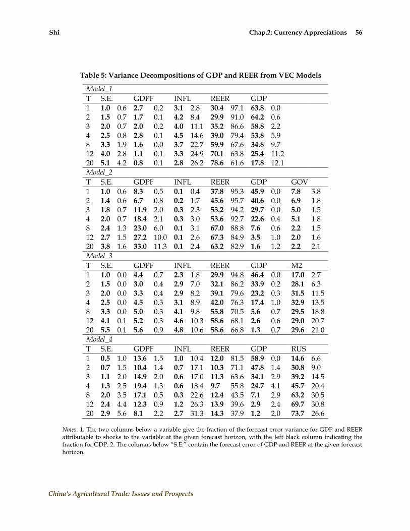
Shi Chap.2: Currency Appreciations 56
China's Agricultural Trade: Issues and Prospects
Table 5: Variance Decompositions of GDP and REER from VEC Models
Model_1
T S.E. GDPF INFL REER GDP
1 1.0 0.6 2.7 0.2 3.1 2.8 30.4 97.1 63.8 0.0 2 1.5 0.7 1.7 0.1 4.2 8.4 29.9 91.0 64.2 0.6 3 2.0 0.7 2.0 0.2 4.0 11.1 35.2 86.6 58.8 2.2 4 2.5 0.8 2.8 0.1 4.5 14.6 39.0 79.4 53.8 5.9 8 3.3 1.9 1.6 0.0 3.7 22.7 59.9 67.6 34.8 9.7 12 4.0 2.8 1.1 0.1 3.3 24.9 70.1 63.8 25.4 11.2 20 5.1 4.2 0.8 0.1 2.8 26.2 78.6 61.6 17.8 12.1 Model_2
T S.E. GDPF INFL REER GDP GOV
1 1.0 0.6 8.3 0.5 0.1 0.4 37.8 95.3 45.9 0.0 7.8 3.8 2 1.4 0.6 6.7 0.8 0.2 1.7 45.6 95.7 40.6 0.0 6.9 1.8 3 1.8 0.7 11.9 2.0 0.3 2.3 53.2 94.2 29.7 0.0 5.0 1.5 4 2.0 0.7 18.4 2.1 0.3 3.0 53.6 92.7 22.6 0.4 5.1 1.8 8 2.4 1.3 23.0 6.0 0.1 3.1 67.0 88.8 7.6 0.6 2.2 1.5 12 2.7 1.5 27.2 10.0 0.1 2.6 67.3 84.9 3.5 1.0 2.0 1.6 20 3.8 1.6 33.0 11.3 0.1 2.4 63.2 82.9 1.6 1.2 2.2 2.1 Model_3
T S.E. GDPF INFL REER GDP M2
1 1.0 0.0 4.4 0.7 2.3 1.8 29.9 94.8 46.4 0.0 17.0 2.7 2 1.5 0.0 3.0 0.4 2.9 7.0 32.1 86.2 33.9 0.2 28.1 6.3 3 2.0 0.0 3.3 0.4 2.9 8.2 39.1 79.6 23.2 0.3 31.5 11.5 4 2.5 0.0 4.5 0.3 3.1 8.9 42.0 76.3 17.4 1.0 32.9 13.5 8 3.3 0.0 5.0 0.3 4.1 9.8 55.8 70.5 5.6 0.7 29.5 18.8 12 4.1 0.1 5.2 0.3 4.6 10.3 58.6 68.1 2.6 0.6 29.0 20.7 20 5.5 0.1 5.6 0.9 4.8 10.6 58.6 66.8 1.3 0.7 29.6 21.0 Model_4
T S.E. GDPF INFL REER GDP RUS
1 0.5 1.0 13.6 1.5 1.0 10.4 12.0 81.5 58.9 0.0 14.6 6.6 2 0.7 1.5 10.4 1.4 0.7 17.1 10.3 71.1 47.8 1.4 30.8 9.0 3 1.1 2.0 14.9 2.0 0.6 17.0 11.3 63.6 34.1 2.9 39.2 14.5 4 1.3 2.5 19.4 1.3 0.6 18.4 9.7 55.8 24.7 4.1 45.7 20.4 8 2.0 3.5 17.1 0.5 0.3 22.6 12.4 43.5 7.1 2.9 63.2 30.5 12 2.4 4.4 12.3 0.9 1.2 26.3 13.9 39.6 2.9 2.4 69.7 30.8 20 2.9 5.6 8.1 2.2 2.7 31.3 14.3 37.9 1.2 2.0 73.7 26.6
Notes: 1. The two columns below a variable give the fraction of the forecast error variance for GDP and REER attributable to shocks to the variable at the given forecast horizon, with the left black column indicating the fraction for GDP. 2. The columns below ―S.E.‖ contain the forecast error of GDP and REER at the given forecast horizon.
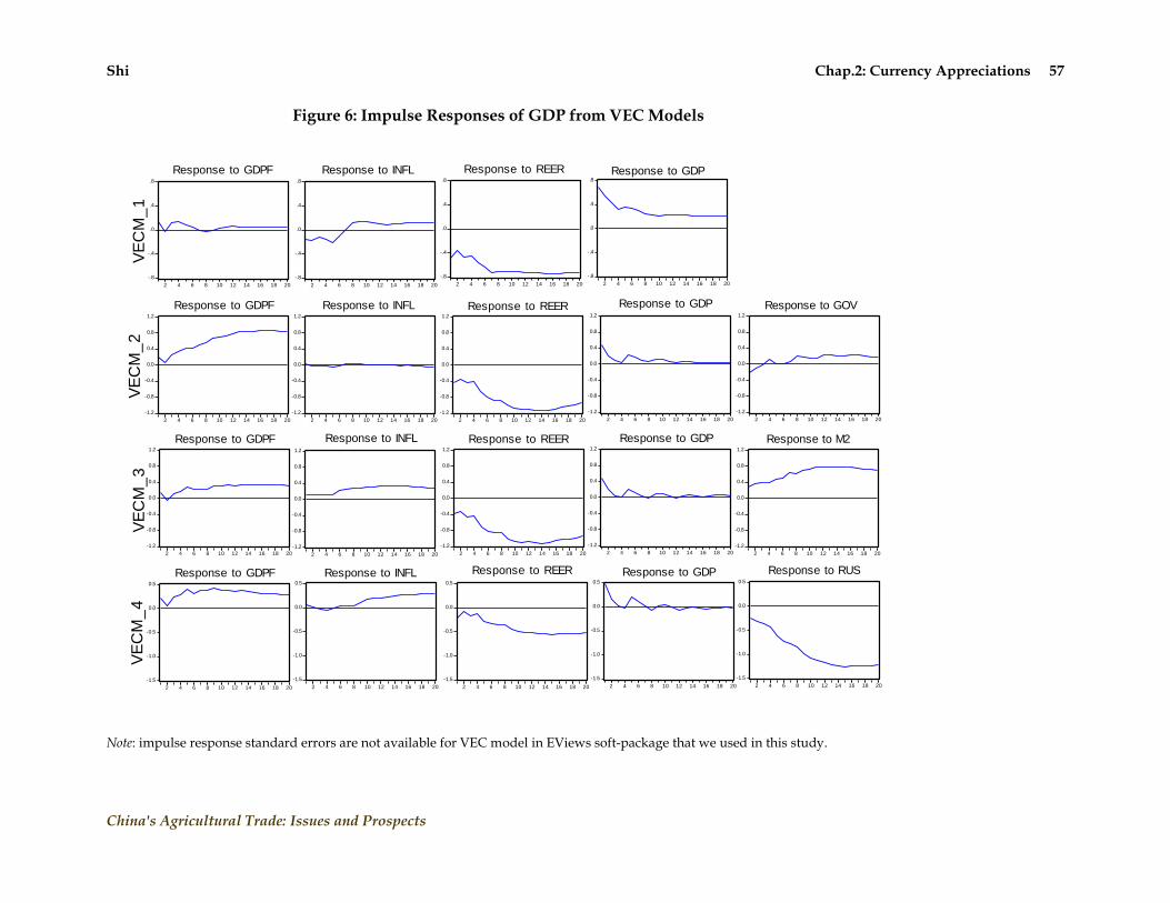
Shi Chap.2: Currency Appreciations 57
China's Agricultural Trade: Issues and Prospects
Figure 6: Impulse Responses of GDP from VEC Models
-.8
-.4
.0
.4
.8
2 4 6 8 10 12 14 16 18 20
Response to GDPF
-.8
-.4
.0
.4
.8
2 4 6 8 10 12 14 16 18 20
Response to INFL
-.8
-.4
.0
.4
.8
2 4 6 8 10 12 14 16 18 20
Response to REER
-.8
-.4
.0
.4
.8
2 4 6 8 10 12 14 16 18 20
Response to GDP
-1.2
-0.8
-0.4
0.0
0.4
0.8
1.2
2 4 6 8 10 12 14 16 18 20
Response to GDPF
-1.2
-0.8
-0.4
0.0
0.4
0.8
1.2
2 4 6 8 10 12 14 16 18 20
Response to INFL
-1.2
-0.8
-0.4
0.0
0.4
0.8
1.2
2 4 6 8 10 12 14 16 18 20
Response to GOV
-1.2
-0.8
-0.4
0.0
0.4
0.8
1.2
2 4 6 8 10 12 14 16 18 20
Response to REER
-1.2
-0.8
-0.4
0.0
0.4
0.8
1.2
2 4 6 8 10 12 14 16 18 20
Response to GDP
-1.2
-0.8
-0.4
0.0
0.4
0.8
1.2
2 4 6 8 10 12 14 16 18 20
Response to GDPF
-1.2
-0.8
-0.4
0.0
0.4
0.8
1.2
2 4 6 8 10 12 14 16 18 20
Response to M2
-1.2
-0.8
-0.4
0.0
0.4
0.8
1.2
2 4 6 8 10 12 14 16 18 20
Response to INFL
-1.2
-0.8
-0.4
0.0
0.4
0.8
1.2
2 4 6 8 10 12 14 16 18 20
Response to REER
-1.2
-0.8
-0.4
0.0
0.4
0.8
1.2
2 4 6 8 10 12 14 16 18 20
Response to GDP
-1.5
-1.0
-0.5
0.0
0.5
2 4 6 8 10 12 14 16 18 20
Response to RUS
-1.5
-1.0
-0.5
0.0
0.5
2 4 6 8 10 12 14 16 18 20
Response to GDPF
-1.5
-1.0
-0.5
0.0
0.5
2 4 6 8 10 12 14 16 18 20
Response to INFL
-1.5
-1.0
-0.5
0.0
0.5
2 4 6 8 10 12 14 16 18 20
Response to REER
-1.5
-1.0
-0.5
0.0
0.5
2 4 6 8 10 12 14 16 18 20
Response to GDP
VE
CM
_1
VE
CM
_2
VE
CM
_3
VE
CM
_4
Note: impulse response standard errors are not available for VEC model in EViews soft-package that we used in this study.

Shi Chap.2: Currency Appreciations 58
China's Agricultural Trade: Issues and Prospects
- with respect to the source of variation in GDP forecast error, in all three new VAR
models, the RUS shocks become the most important and predominant source of variation in
GDP, while, in contrast, REER shocks turn out to be the second, the third, and the fourth most
important sources of the GDP error variance, respectively. The contributions of ―own shocks‖
and M2 to variation in GDP exceed the contribution of REER in the second and third new
models; and
Table 6: Variance Decompositions of GDP from VAR Models with RUS
Model_1
T S.E. RUS INFL REER GDP
1 0.5 6.8 0.1 24.4 68.8 2 0.8 10.1 3.7 23.4 62.8 3 0.9 13.7 6.0 26.2 54.18 4 1.0 18.2 6.4 25.8 49.6 8 1.2 46.9 2.7 26.9 23.6 12 1.4 58.0 2.3 23.4 16.2 20 1.7 55.7 4.7 20.1 19.6 Model_2
T S.E. RUS INFL REER GDP GOV
1 0.6 8.0 0.0 26.6 63.1 2.3 2 0.8 9.8 5.9 23.9 58.7 1.7 3 0.9 13.0 10.3 25.2 49.9 1.5 4 1.0 16.5 11.4 24.3 44.4 3.4 8 1.2 42.8 7.0 23.4 23.7 3.1 12 1.3 59.1 4.7 17.6 16.2 2.4 20 1.6 54.9 7.6 16.5 19.0 2.1
Model_3
T S.E. RUS INFL REER GDP M2
1 0.5 7.8 0.1 22.3 59.6 10.2 2 0.8 8.6 0.8 18.3 48.4 23.9 3 0.9 11.7 2.2 18.9 39.9 27.3 4 1.0 14.5 2.5 18.3 36.3 28.4 8 1.1 42.9 1.6 16.7 20.1 18.7 12 1.3 60.6 1.1 11.7 13.6 13.0 20 1.6 57.9 1.9 12.1 14.3 13.9
Note: 1. The column below a variable gives the fraction of the forecast error variance for GDP that is attributable to shocks to the variable at the given forecast horizon. 2. The column below ―S.E.‖ contains the forecast error of GDP at the given forecast horizon.

Shi Chap.2: Currency Appreciations 59
China's Agricultural Trade: Issues and Prospects
Figure 7: Impulse Responses of GDP from VARs with RUS Substituting for GDPF
-1.2
-0.8
-0.4
0.0
0.4
0.8
2 4 6 8 10 12 14 16 18 20
Response to RUS
-1.2
-0.8
-0.4
0.0
0.4
0.8
2 4 6 8 10 12 14 16 18 20
Response to INFL
-1.2
-0.8
-0.4
0.0
0.4
0.8
2 4 6 8 10 12 14 16 18 20
Response to REER
-1.2
-0.8
-0.4
0.0
0.4
0.8
2 4 6 8 10 12 14 16 18 20
Response to GDP
-1.2
-0.8
-0.4
0.0
0.4
0.8
2 4 6 8 10 12 14 16 18 20
Response to RUS
-1.2
-0.8
-0.4
0.0
0.4
0.8
2 4 6 8 10 12 14 16 18 20
Response to INFL
-1.2
-0.8
-0.4
0.0
0.4
0.8
2 4 6 8 10 12 14 16 18 20
Response to GOV
-1.2
-0.8
-0.4
0.0
0.4
0.8
2 4 6 8 10 12 14 16 18 20
Response to REER
-1.2
-0.8
-0.4
0.0
0.4
0.8
2 4 6 8 10 12 14 16 18 20
Response to GDP
-1.2
-0.8
-0.4
0.0
0.4
0.8
2 4 6 8 10 12 14 16 18 20
Response to RUS
-1.2
-0.8
-0.4
0.0
0.4
0.8
2 4 6 8 10 12 14 16 18 20
Response to M2
-1.2
-0.8
-0.4
0.0
0.4
0.8
2 4 6 8 10 12 14 16 18 20
Response to INFL
-1.2
-0.8
-0.4
0.0
0.4
0.8
2 4 6 8 10 12 14 16 18 20
Response to REER
-1.2
-0.8
-0.4
0.0
0.4
0.8
2 4 6 8 10 12 14 16 18 20
Response to GDP
Mo
de
l_1
Mo
de
l_2
Mo
de
l_3
Shi Chap.2: Currency Appreciations 60
China's Agricultural Trade: Issues and Prospects
(4) The effects of other shocks on GDP are similar between the new models and the original
ones. Figure 7 and Table 6 provide IRFs and variance decompositions of GDP from the three
new VAR models, with RUS replacing GDPF as a proxy variable for external shocks.
In sum, the robustness analysis confirms that the basic result - shocks to the RMB real
exchange rate have a contractionary effect on China‘s output - does not change even if the
orderings of Kamin and Rogers (2000) are adopted or a VEC model specification is used.
However, after including the international finance linkage of the Chinese economy, the effect of
the REER shock on China‘s output and the power of REER shocks in explaining changes in
China‘s output turn out to be relatively small, while U.S. interest rate shocks have a relatively
large effect on China‘s output, such that the magnitude of it exceeds that of RMB exchange rate
shocks.
Conclusion
This chapter investigates the relationship between the RMB real exchange rate and China‘s
output by using the VAR model technique. The empirical analysis reveals several interesting
findings. First, even after the source of spurious correlation is controlled for, RMB real exchange
rate appreciation leads to a decline in China‘s output, suggesting that currency appreciations
have been contractionary in China, as suggested by traditional open economy macroeconomics.
Second, when the international finance linkages of the Chinese economy are accounted
for, the effect of RMB real exchange rate shocks on China‘s output and the power of the shocks
in explaining the change in China‘s output are relatively small, while the effect of U.S. interest
rate shocks on China‘s output is relatively large. The intuition behind this finding is that the
effectiveness of China‘s capital controls has eroded over time and the scales of capital inflows
and outflows have become large enough such that external shocks through international
financial channels have a significant influence on the Chinese economy, which exceeds the
influence of external shocks through international trade channels.
Third, besides shocks to the RMB real exchange rate and the U.S. interest rate, shocks to
domestic money supply and foreign demand have important effects on China‘s output.
However, government spending shocks have less power in explaining changes in China‘s
output.
Shi Chap.2: Currency Appreciations 61
China's Agricultural Trade: Issues and Prospects
The conclusion that currency appreciations are contractionary in China is remarkably
different from those made by similar empirical work on developing countries. The possible
explanations for this difference are outlined below:
- first, in the existing research on the ―contractionary devaluations‖ effect in developing
countries, devaluations usually take place under an abnormal environment of currency or
financial crisis and thus have been associated with economic recession, but RMB devaluations
did not happen in the case of currency or financial crisis until now;
- second, urban economic reform begun in the early 1990s has caused many people to lose
their jobs and traditional benefits, such as healthcare, pensions, and education. In turn, this has
strengthened the motive for precautionary savings in households in urban and township areas.
Therefore, the income reallocation effect as well as the real cash balance and the real wealth
effects of currency appreciation may not play a very great role;
- third, China has absorbed a large amount of foreign direct investment for many years. As
a result, the technological progress and production capacity of China‘s manufacturing industry
have been promoted rapidly, the substitutability of home-produced capital goods (including
those produced by foreign investment enterprises) for imported goods has been strengthened
and, therefore, the effect of the RMB real exchange rate on domestic investment spending is not
clear;
- fourth, one condition under which devaluation can lead to a reduction in national output
is that imports initially exceed exports (Krugman and Taylor, 1978). China‘s trade balance has
been in surplus for more than 10 years, except for 1993, and therefore does not satisfy that
condition;
- finally, because of the characteristics of processing trade in China‘s manufacturing
industry, as well as the administrative controls on prices (especially in the service sector), the
supply-side effect of the RMB exchange rate on output is also uncertain. In short, it seems that
the expenditure-changing effect and supply-side effect of RMB exchange rate changes have not
been that remarkable in practice until now. Therefore, the effect of RMB real exchange rate
shocks on China‘s output is mainly embodied in the expenditure-switching effect as
emphasized by traditional macroeconomic theory. Consequently, appreciations in the RMB are
likely contractionary.

Shi Chap.2: Currency Appreciations 62
China's Agricultural Trade: Issues and Prospects
It is worth pointing out however, that concluding that appreciations have been
contractionary in China does not necessarily mean that China should continue maintaining an
undervalued exchange rate, since the value of the RMB has already caused the Chinese
economy to run into internal and external imbalances in the past several years. Figure 2 (above)
shows that China‘s real GDP has been running above its long-term trend since 2003, and this
kind of deviation is expanding. Indeed, overheating of the Chinese economy is obvious.
Undoubtedly, continuing undervaluation of the RMB will further aggravate imbalances in the
Chinese economy. On the other hand, the conclusion that appreciations have been
contractionary in China implies that relative to other effects of changes in the exchange rate, the
expenditure-switching effect has been predominant in China until now. Hence, it is effective to
use the orthodox Swan Diagram to analyze macroeconomic policy issues in China. According
to the Swan Diagram, allowing the RMB to appreciate will be helpful to the Chinese economy in
realizing internal and external balances (Shi, 2006).
Additionally, in recent years China‘s capital account surplus has increased rapidly along
with increases in the current account surplus. The rapid increase in the ―double surplus‖ has
caused China‘s foreign exchange reserves to expand in an uncontrolled manner. In addition,
the money supply and domestic credit have expanded passively, aggravating overheating of the
Chinese economy and the difficulties for the Chinese government's macroeconomic
management. In particular, as China‘s capital account is gradually liberalized and the
effectiveness of capital controls erodes over time, ―hot money‖ flows into China will expand,
becoming a major reason for rapid expansion of foreign exchange reserves.
The empirical work indicates that the effect of shocks on China‘s output through
international financial channels (as represented by U.S. interest rate shocks) exceeds that of
international trade channels (as represented by RMB real exchange rate shocks), suggesting it is
important for the Chinese authorities to handle the capital inflow problem correctly. The inflow
of ―hot money‖ in recent years is mainly a response to expectation of RMB appreciation, and an
important reason for the persistent existence of these expectations is undervaluation of the
RMB. Therefore, allowing the RMB to appreciate at a faster rate towards its equilibrium will
lessen expectations of RMB appreciation, thus relaxing pressure on the Chinese authorities due
to the rapid increase in foreign exchange reserves.
Shi Chap.2: Currency Appreciations 63
China's Agricultural Trade: Issues and Prospects
References
Akinlo, A.E, and A.F. Odusola. ―Assessing the Impact of Nigeria‘s Naira Depreciation on Output and Inflation,‖ Applied Economics 35 (2003): 691-703.
Berument, H. and M. Pasaogullari. ―Effects of the Real Exchange Rate on Output and Inflation: Evidence from Turkey,‖ The Developing Economies 41(2003): 401–35.
Branson W.H. ―Stabilization, Stagflation, and Investment Incentives: The Case of Kenya, 1979-1980.‖ In Economic Adjustment and Exchange Rates in Developing Countries, S. Edwards and L. Ahamed (eds.). Chicago, IL: Chicago University Press (1986).
Bruno, M. ―Stabilization and Stagflation in a Semi-Industrialized Economy.‖ In International Economic Policy: Theory and Evidence, R. Dornbusch and J.A. Frankel (eds.). Baltimore, MA: John Hopkins University Press (1979).
Caves, R.E., J.A. Frankel, and R.W. Jones. World Trade and Payments: An Introduction. Reading, MA: Addison-Wesley (2002).
Cochrane,J. H. Time Series for Macroeconomics and Finance, Manuscript, University of Chicago (2005).
Cooper, R. N. ―Currency Devaluation in Developing Countries.‖ In Government and Economic Development, G. Ranis (ed.). New Haven, CT: Yale University Press (1971).
Coudert, V. and C. Couharde. ―Real Equilibrium Exchange Rate in China,‖ CEPII Working Paper No. 2005 – 01. Paris: CEPII (2005).
Diaz-Alejandro, C. F. ―A Note on the Impact of Devaluation and the Redistributive Effects,‖ Journal of Political Economy 71(1963): 577–580.
Edwards, S. ―Are Devaluations Contractionary?‖ The Review of Economics and Statistics 68 (1986): 501-508.
Frankel, J. A. ―On the Yuan: The Choice between Adjustment under a Fixed Exchange Rate and Adjustment under a Flexible Rate,‖ IMF Seminar Paper. Dalian, China (May 26–27, 2004).
Frankel, J. A. ―Mundell-Fleming Lecture:Contractionary Currency Crashes in Developing Countries,‖ IMF Staff Papers 52 (2005): 149-192.
Goldstein, M. 2004. ―Adjusting China‘s Exchange Rate Policies,‖ IMF Seminar Paper. Dalian, China (May 26-27, 2004).
Gylfason, T. and M. Radetzki. ―Does Devaluation Make Sense in the Least Developed Countries?‖ Economic Development and Cultural Change 40 (1991): 1–25.
Hirschman, A. O. ―Devaluation and the Trade Balance:A Note,‖ The Review of Economics and Statistics 31 (1949): 50-53.
Hoffmaister, A. W. and C. A. Vegh. ―Disinflation and the Recession-Now-Versus- Recession-Later Hypothesis: Evidence from Uruguay,‖ IMF Staff Papers 43 (1996): 355-394.
Johansen,S. Likelihood-Based Inference in Cointegrated Vector Autoregressive Models. Oxford: Oxford University Press (1995).
Kamin, S. B. and J. H. Rogers. ―Output and the Real Exchange Rate in Developing Countries: An Application to Mexico,‖ Journal of Development Economics 61 (2000): 85–109.
Krugman, P. and L. Taylor. ―Contractionary Effects of Devaluation‖, Journal of International Economics 8 (1978): 445–456.
Lizondo, J.S. and P. J. Montiel. ―Contractionary Devaluation in Developing Countries: An Analytical Overview,‖ IMF Staff Papers 36 (1989): 182–227.
Moreno, R. 1999. ―Depreciations and Recessions in East Asia,‖Federal Reserve Bank of San Francisco Economic Review 3(1999): 27–40.
Shi Chap.2: Currency Appreciations 64
China's Agricultural Trade: Issues and Prospects
Obstfeld, M. and K. Rogoff. ―Exchange Rate Dynamics Redux,‖ Journal of Political Economy, 103 (1995): 624-660.
Shi, J. ―Adjustment of Global Imbalances and Its Impact on China‘s Economy,‖ China and World Economy 14 (2006): 71-85.
Shi, J. and H. Yu. ―Renminbi Equilibrium Exchange Rate and China‘s Exchange Rate Misalignment: 1991-2004,‖ Economic Research Journal 40 (2005): 34-45.
Sims, C. ―Macroeconomics and Reality,‖ Econometrica 48 (1980): 1–48. Sims, C., J. Stock, and M. Watson. ―Inference in Linear Time Series Models with Some Unit
Roots,‖ Econometrica 58 (1990): 113–44. Van Wijnbergen S. V. 1986. ―Exchange Rate Management and Stabilization Policies in
Developing Countries,‖ Journal of Development Economics 23 (1986): 227-247.
Gale Chap.3: A Tale of Two Commodities 65
China's Agricultural Trade: Issues and Prospects
Chapter 3:
A Tale of Two Commodities: China’s Trade in Corn and Soybeans
FRED GALE
Economic Research Service, USDA

Gale Chap.3: A Tale of Two Commodities 66
China's Agricultural Trade: Issues and Prospects
Chapter 3:
A Tale of Two Commodities: China’s Trade in Corn and Soybeans*
Introduction
It was the best of times, and the worst of times. It was a time of great expectations, dashed
hopes, and surprising plot twists. It was the five-year period following China‘s December 2001
accession to the World Trade Organization (WTO).
Nearly all analysts predicted that China‘s agricultural imports would rise sharply after it
joined the WTO. The United States (U.S.) and other agricultural exporting countries anticipated
―the best of times‖ after WTO accession as China lowered barriers, experienced faster growth,
and increased its imports of grains, oilseeds, and livestock products (Lohmar, Hansen, Hsu, and
Seeley, 2002). Many analysts in China anticipated ―the worst of times‖ for the country‘s small
farmers who would be unable to compete with low-priced imported commodities from
developed countries.
At first glance, the projections appear to have been correct. China‘s agricultural imports
(using the United States Department of Agriculture‘s (USDA‘s) definition which excludes fish
and forest products) nearly tripled from $10.5 billion in 2001 to $30.6 billion in 2006 (Figure 1).
However, a closer look reveals that China‘s agricultural trade did not evolve quite as expected.
Most analysts expected a broad-based increase in imports of grains, other field crops, meat, and
dairy products but the growth in imports, has been concentrated in a narrow range of
commodities. It was ―the best of times‖ for U.S. soybean and cotton exporters. Soybeans and
cotton combined accounted for nearly half of the $20 billion increase in China‘s agricultural
imports from 2001 to 2006 (Table 1). Natural rubber and palm oil accounted for another one-
fifth of the import growth. That means 70% of the growth in China‘s agricultural imports came
from just four commodities.1
* The views expressed here are those of the author, and may not be attributed to the Economic Research Service or the
U.S. Department of Agriculture. The author thanks Francis Tuan, Bryan Lohmar, Ed Allen, Steve MacDonald, Rick O‘Meara, William Tierney, and Mary Anne Normile for providing comments on earlier drafts of the paper. 1 Other descriptions of China‘s recent agricultural trade trends can be found in Gale (2005, 2007), Tian (2006), and Bao (2007).

Gale Chap.3: A Tale of Two Commodities 67
China's Agricultural Trade: Issues and Prospects
Figure 1: China’s Agricultural Imports and Exports, 1995-2006
It was ―the worst of times‖ for those predicting that China would import corn and wheat.
Much of the ex ante analysis of WTO impacts focused on the potential for grain imports, yet
cereal imports accounted for less than 2% of China‘s agricultural import growth. Projections of
China‘s transition to corn net importer are consistently pushed further into the future. China‘s
wheat imports also failed to meet expectations.
The surge in agricultural imports has not led to ―the worst of times‖ for Chinese farmers.
The imports that have grown the most are commodities that do not compete directly with
products of most Chinese farmers. Natural rubber and palm oil are tropical products not
produced in significant quantities in China. Vegetable and fruit imports consist mainly of
cassava and tropical fruits from Southeast Asia. Imports of apples and citrus occupy high-end
market niches and do not compete directly with Chinese fruit.
There have been complaints about imports from domestic soybean and cotton growers, but
demand for these commodities has grown so strongly that production and prices for these
commodities did not decline despite the flood of imports. In addition, many Chinese farmers
benefited from improved export opportunities. China‘s agricultural exports grew at a steady
pace, just slightly slower than imports.
0
5
10
15
20
25
30
35
1995 1996 1997 1998 1999 2000 2001 2002 2003 2004 2005 2006
Billion dollars
Imports
Exports
Source: ERS calculations using China Customs Statistics Note: Definition of ―agricultural‖ excludes fish and forest products and includes unprocessed cotton, wool, and animal hides

Gale Chap.3: A Tale of Two Commodities 68
China's Agricultural Trade: Issues and Prospects
Table 1: Composition of China’s Agricultural Import Growth, 2001-06
HS codes Commodity
Change,
2001-06 Share of change
$million %
NA All agricultural* 20,071 100.0
5201 Cotton 4,797 23.9
1201 Soybeans 4,680 23.3
4001 Natural rubber 2,438 12.1
1511 Palm oil 1,871 9.3
1507 Soybean oil 779 3.9
07, 08 Fruits and vegetables 917 4.6
41 Animal hides and skins 761 3.8
5101 Wool 470 2.3
04 Dairy products 346 1.7
10 Cereals 213 1.1
Other agricultural 2,798 13.9
Source: Author‘s calculations using China Customs Statistics reported by World Trade Atlas *Agricultural includes HS codes 01-20, excluding fish and seafood, plus unprocessed animal hides, cotton, and wool Note: Table shows change in calendar-year agricultural imports between 2001 and 2006
Five years after WTO accession, China maintained its self-sufficiency in traditional staple
crops while its reliance on imports of soybeans and cotton increased sharply. Calculations based
on USDA/Foreign Agriculture Service (FAS) estimates show that China‘s ratio of domestic
production to consumption for rice, wheat and corn rose from 80-90% in 2003 to 100% or higher
in 2006 (Table 2). China is also near self-sufficiency in rapeseed. In 2006, China‘s soybean
production met only 35% of its consumption and its cotton production met 75%.
Two Commodities: Corn and Soybeans
The remainder of this chapter looks more carefully at China‘s trade in two commodities—corn
and soybeans—that followed contrasting trends in trade. The corn-soybean story illustrates
how China‘s actual trade patterns do not always follow trends predicted by economists based
on fundamental tariff and price relationships.
Corn and soybeans are both land-extensive crops in which China does not have a
comparative advantage. Both commodities were traditionally staple food grains in China, but
are now used primarily for animal feed and cooking oil. Soybean imports were liberalized in
the 1990s to encourage livestock industry development. Corn remains a strategic commodity
since it is still considered by many policymakers to be a staple grain and is widely grown by

Gale Chap.3: A Tale of Two Commodities 69
China's Agricultural Trade: Issues and Prospects
Chinese farmers (corn output is nearly 10 times soybean output in China). It is the primary crop
in northeastern provinces which were hit hard by economic restructuring in the 1990s.
Table 2: China Self-Sufficiency in Major Crops, 1996-06
Year Rice Wheat Corn Rapeseed Soybeans Cotton
----------------------------%-------------------------
1996 103 103 121 100 92 100
1997 106 113 95 97 95 114
1998 104 101 117 79 76 115
1999 104 104 109 73 62 86
2000 98 90 88 83 58 89
2001 91 86 93 94 54 96
2002 90 86 96 100 47 78
2003 85 83 90 96 45 72
2004 96 90 99 98 43 83
2005 99 96 102 95 37 68
2006 100 103 102 93 35 75
Source: ERS calculations based on USDA/FAS, PSD Note: Table shows ratio of domestic production to domestic consumption. Inventories are not considered in the calculation
Studies conducted in the 1990s found positive rates of protection for both commodities
(Martin, 2003; Huang, Chen, Rozelle, and Tuan, 2003). At the time of WTO accession, China‘s
domestic prices for corn and soybeans were both well above U.S. prices. The price of soybeans
in China‘s main production area (Heilongjiang Province) was 32% above the U.S. farm price
(Figure 2), while the corn price in China‘s corn production areas (Jilin Province) was 47% above
the U.S. farm price (Figure 3). Domestic Chinese prices of corn and soybeans are higher in
coastal areas where many of China‘s feed mills and oilseed-crushing plants are located.
After WTO accession, imports of both soybeans and corn were subject to low tariffs.
Soybean imports were assessed only a 3% tariff with no quota on imports, a regime that was in
place before WTO accession. For corn, China agreed to set annual tariff rate quotas (TRQs) after
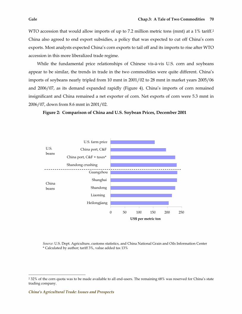
Gale Chap.3: A Tale of Two Commodities 70
China's Agricultural Trade: Issues and Prospects
WTO accession that would allow imports of up to 7.2 million metric tons (mmt) at a 1% tariff.2
China also agreed to end export subsidies, a policy that was expected to cut off China‘s corn
exports. Most analysts expected China‘s corn exports to tail off and its imports to rise after WTO
accession in this more liberalized trade regime.
While the fundamental price relationships of Chinese vis-á-vis U.S. corn and soybeans
appear to be similar, the trends in trade in the two commodities were quite different. China‘s
imports of soybeans nearly tripled from 10 mmt in 2001/02 to 28 mmt in market years 2005/06
and 2006/07, as its demand expanded rapidly (Figure 4). China‘s imports of corn remained
insignificant and China remained a net exporter of corn. Net exports of corn were 5.3 mmt in
2006/07, down from 8.6 mmt in 2001/02.
Figure 2: Comparison of China and U.S. Soybean Prices, December 2001
Source: U.S. Dept. Agriculture, customs statistics, and China National Grain and Oils Information Center * Calculated by author; tariff 3%, value added tax 13%
2 32% of the corn quota was to be made available to all end-users. The remaining 68% was reserved for China‘s state trading company.
0 50 100 150 200 250
Heilongjiang
Liaoning
Shandong
Shanghai
Guangzhou
Shandong crushing plant
China port, C&F + taxes*
China port, C&F
U.S. farm price
US$ per metric ton
U.S.
beans
China
beans

Gale Chap.3: A Tale of Two Commodities 71
China's Agricultural Trade: Issues and Prospects
Figure 3: Comparison of China and U.S. Corn Prices, December 2001
Source: U.S. Dept. Agriculture and China National Grain and Oils Information Center *Calculated by author; tariff assumed 1%, value added tax 13%
Did China protect its corn market from imports? Apart from tariffs, China utilized several
other measures that may have protected domestic commodities. One major policy is the
differential treatment of domestic and imported commodities for assessing the 13-percent value
added tax (VAT). The VAT is assessed on the gross value of imported commodities, but Latner
and Jiang‘s (2007) analysis suggests that domestic commodities are assessed a lower effective
rate due to exemptions for farmers and several categories of farm inputs.3 The VAT policy
affects both corn and soybeans equally and does not explain the divergent trends in trade
between the two commodities. VAT rebates for exports (used mostly for corn) appear to be a de
facto export subsidy. Delays in approving genetically-modified corn events and distribution of
tariff rate quotas in small lots may have constrained corn imports. Domestic policies that
induced farmers to plant more grain beginning in 2004 and good weather increased domestic
3 Imports of several other types of animal feeds including fish meal, bran, distillers dried grains, and rapeseed meal are exempt from VAT (Latner and Jiang, 2007) and the VAT is sometimes waived for other commodities on an ad hoc basis.
0 50 100 150
Jilin
Dalian
Guangzhou
U.S. gulf + freight + taxes*
U.S. gulf + freight*
U.S. gulf
U.S. farm price
US$ per metric ton
U.S.
corn
China corn

Gale Chap.3: A Tale of Two Commodities 72
China's Agricultural Trade: Issues and Prospects
supplies of corn. High ocean freight rates increased C&F prices of U.S. corn in Asia, but this
factor also affected soybeans.
Figure 4: China Net Imports of Soybeans and Corn, 2000-2007
Monthly domestic and border prices were compared over the period from 2002 to 2007 to
assess the degree of protection of the corn and soybean markets. Monthly domestic wholesale
prices by province were obtained from China National Grain and Oils Information Center, and
converted to U.S. dollars at the official exchange rate for the corresponding month. In Figures 5
and 6, domestic prices are shown for a production area - Heilongjiang Province for soybeans
and Jilin for corn - and for a coastal province - Shandong Province for soybeans and Guangdong
for corn. The border price for soybeans was calculated as the average unit value of imported
soybeans reported in China customs statistics. It was not possible to calculate an actual import
price for corn since China imported little or no corn during this period. The unit value of
-20
-10
0
10
20
30
40
2000/01 2001/02 2002/03 2003/04 2004/05 2005/06 2006/07
Million Metric
Tons
Soybeans
Corn
Source: USDA/FAS, PSD Note: Data are for market years October - September

Gale Chap.3: A Tale of Two Commodities 73
China's Agricultural Trade: Issues and Prospects
Taiwan corn imports was used to approximate the price at the Chinese border.4 These border
prices do not include tariffs or VAT.
Domestic prices of both corn and soybeans were above border prices for most months of
the period 2002-07 suggesting a modest level of protection. The border price of soybeans was
consistently below the coastal (Shandong) domestic price, and usually below the price in inland
production areas (Heilongjiang). The monthly differential between the Shandong price and the
border price averaged 21% over the period 2002-07, and it ranged mostly between 10 and 30%.
After adding the tariff and value added tax, the cost of imported soybeans was still slightly
below the domestic price in Shandong in most months. The border (Taiwan) price for corn was
below the coastal (Guangdong) domestic price during most months of the period 2002-07, but
there were periods during 2003 and 2004 when the border price was at or above the domestic
price. After adding the tariff and value added tax, the theoretical price of imported corn was at
or above the Guangdong price during most of 2002-07.
Figure 5: China Soybeans--Domestic and Border Prices, 2002-07
4 A border price was also calculated by adding average shipping costs (U.S. Gulf to East Asia) to the average U.S. Gulf ports price of corn. This measure seemed consistent with the Taiwan unit value.
0
100
200
300
400
500
600
1-02 5-02 9-02 1-03 5-03 9-03 1-04 5-04 9-04 1-05 5-05 9-05 1-06 5-06 9-06 1-07
US$/MT Domestic Coastal
Domestic Production Area
China Border Price
Illinois Farm Price
Source: China National Grain and Oils Information Center; China Customs Statistics

Gale Chap.3: A Tale of Two Commodities 74
China's Agricultural Trade: Issues and Prospects
The co-movements between prices reveal differences in liberalization of the corn and
soybean markets in China. Fluctuations in domestic soybean prices appear very closely
correlated with fluctuations in the border price, an indicator that international market
conditions are transmitted to the China market. Domestic soybean prices in coastal and
production regions of China move almost in unison, suggesting that price changes in one region
are quickly transmitted to other regions. By implication, international market changes are
quickly transmitted to markets in soybean production areas.
Figure 6: China Corn—Domestic and Border Prices, 2002-07
Sources: China National Grain and Oils Information Center and Taiwan Customs Statistics
Price trends for corn suggest that China‘s corn market is more insulated from the world
market. Like domestic soybean prices, domestic corn prices in production areas (Jilin) and
coastal areas (Guangdong) move together very closely, suggesting that domestic markets are
closely integrated. However, domestic corn prices are not as closely linked to trends in
international prices. Sharp peaks in the border price of corn in 2004 and early 2007 are reflected
by contemporaneous—but much less pronounced—peaks in Chinese prices, suggesting that
shocks to the world market do have some impact on the Chinese market. However, during
other periods (2002-03, 2005, and early 2006), there appears to be little co-movement between
0
50
100
150
200
250
2002 2003 2004 2005 2006 2007
US$/MT
Domestic coastal
Domestic production area
Border price (Taiwan)

Gale Chap.3: A Tale of Two Commodities 75
China's Agricultural Trade: Issues and Prospects
Chinese and international corn prices. These recent price trends suggest that the Chinese corn
market is more insulated from the international market than is the soybean market.
One of the major differences between China‘s corn and soybean markets during this period
was government stock-holding. China held large government reserves of corn accumulated
during the 1990s, but it did not hold large soybean reserves. The soybean market was driven by
current-year production and consumption and world prices, but the corn market was
dominated by the problem of disposing of huge corn stocks without depressing domestic
market prices. China sought to create new demand by developing livestock production, starch,
and ethanol industries in corn production areas. The most important means of disposing of corn
stocks was subsidized exports. The relatively stable domestic corn prices in China suggest that
authorities succeeded in stabilizing the domestic corn market. However, stability came at great
financial cost.
Figure 7: China Corn: Domestic and Export Prices, 2002-07
Source: China National Grain and Oils Information Center; China Customs Statistics
China agreed to end subsidies for exports after WTO accession, but corn export sales
continued to be made at prices well below domestic prices after WTO accession (Figure 7).5
5 China now claims to offer only a rebate of VAT and waivers of rail taxes. Only two companies are authorized to export Chinese corn, and they must have quotas awarded by the central government to do so. The export price
0
50
100
150
200
250
2002 2003 2004 2005 2006 2007
US$/MT
Domestic price
FOB export price

Gale Chap.3: A Tale of Two Commodities 76
China's Agricultural Trade: Issues and Prospects
Since 2002, the unit value of corn exports has generally been 10%-20% below the wholesale
price at Dalian in Liaoning Province, the main port for shipments of northeastern corn both to
export markets and corn deficit areas in southern China. On average, the monthly average unit
value of exports was $24 below the domestic price at Dalian. Calculations based on China
customs statistics show that China exported a cumulative total of 42 million metric tons of corn
during 2002-06.6 These figures suggest that the total subsidy cost of corn exports over the period
2002-06 was roughly $1 billion (Table 3). The policy implicitly taxed feed and livestock
producers in southern China, but those costs are difficult to quantify.
Table 3: Estimated Subsidy Cost, Chinese Corn Exports, 2002-06
Unit Total
Cumulative exports Million metric
tons
42
Estimated subsidy per ton* Dollars per
metric ton
24
Estimated total cost** Dollars 1 billion
Source: Author‘s calculations based on data from China Customs Statistics and China National Grain and Oils Information Center *Average difference between value per ton of exports and domestic price at Dalian. ** (Cumulative exports) x (subsidy per ton)
Over the five-year period 2002-06 (calendar years) China‘s net imports of soybeans totaled
105 mmt while exports of corn totaled 42 mmt. This policy has the appearance of supporting
corn prices while allowing soybean prices to fall. In fact, there has been some agitation among
soybean interests to protect local farmers from imported beans. Lan (2006) painted a bleak
scenario of soybean farmers unable to sell their crops, and attributed their problems to
competition from imported soybeans. The Ministry of Agriculture (2006, p. 110) identified the
increase in soybean imports as an adverse effect of WTO accession that prevented prices and
farm incomes from rising.
In fact, soybean imports have not driven down soybean prices—either in absolute terms or
relative to corn. Soybean prices increased faster than corn prices from 2002 to 2004, before
exceeded the domestic price during 2004 when subsidized exports were suspended due to tight domestic grain market conditions. 6 The cumulative corn export total for the decade from 1997 to 2006 was 74 million metric tons.

Gale Chap.3: A Tale of Two Commodities 77
China's Agricultural Trade: Issues and Prospects
falling during 2004-06 (Figure 8). Over the entire 2002-2007 period there was no long-term
decline in soybean prices. By comparison, corn prices were relatively stable over that period.
According to cost of production survey data collected by the National Development and
Reform Commission Department of Price (2006), farm profits from both corn and soybean rose
in 2003-05 (Figure 9).
Figure 8: Comparison of Domestic Soybean and Corn Prices, Monthly 2002-07
Chinese farmers did not abandon soybeans or corn after WTO accession. Soybean area
remained at slightly less than 10 million hectares, and China‘s planted area in corn rose to an
historical high in 2005 of 26.4 million hectares, exceeding the previous historical high reached in
1999 (Figure 10). The rise in corn area did not result in a large decline in soybean area.7
7 Planting intentions surveys indicate that there was a shift in area from corn to soybeans in 2007.
0
100
200
300
400
500
600
1-01 7-01 1-02 7-02 1-03 7-03 1-04 7-04 1-05 7-05 1-06 7-06 1-07
US$/MT
Soybeans
Corn
Source: China National Grain and Oils Information Center
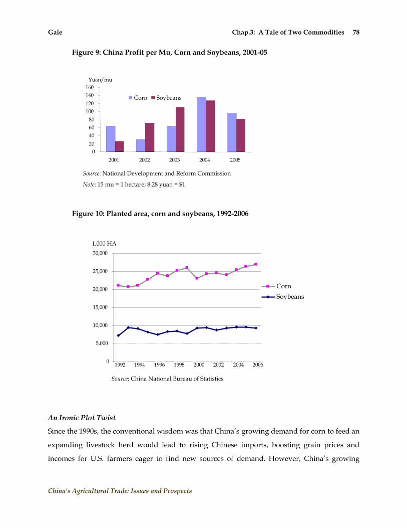
Gale Chap.3: A Tale of Two Commodities 78
China's Agricultural Trade: Issues and Prospects
Figure 9: China Profit per Mu, Corn and Soybeans, 2001-05
Figure 10: Planted area, corn and soybeans, 1992-2006
An Ironic Plot Twist
Since the 1990s, the conventional wisdom was that China‘s growing demand for corn to feed an
expanding livestock herd would lead to rising Chinese imports, boosting grain prices and
incomes for U.S. farmers eager to find new sources of demand. However, China‘s growing
0
20
40
60
80
100
120
140
160
2001 2002 2003 2004 2005
Yuan/mu
Corn Soybeans
Source: National Development and Reform Commission
Note: 15 mu = 1 hectare; 8.28 yuan = $1
0
5,000
10,000
15,000
20,000
25,000
30,000
1992 1994 1996 1998 2000 2002 2004 2006
1,000 HA
Corn
Soybeans
Source: China National Bureau of Statistics

Gale Chap.3: A Tale of Two Commodities 79
China's Agricultural Trade: Issues and Prospects
demand emerged in the form of soybean imports that grew beyond most forecasters‘
expectations. China‘s corn imports have not yet materialized.
In 2006 and 2007, ―the best of times‖ finally emerged for U.S. corn producers. The Illinois
farm price for corn surpassed $3.50 per bushel in 2007, up from less than $2 per bushel at the
time of China‘s WTO accession. The new source of corn demand emerged not in China, but in
the United States, in the form of the U.S. ethanol boom.
The irony is that new demand for corn in the U.S. affected the China market, not the other
way around. Prior to the ethanol boom, China‘s corn prices were rising gradually in 2005 and
2006, reflecting a tightening of Chinese corn markets as corn stocks diminished and industrial
demand for corn expanded. Several Chinese feed and starch companies imported 62,000 metric
tons of U.S. corn in the first half of 2006 to test the mechanism for importing grain. No further
purchases were made after the sharp rise in U.S. prices in Sept-Nov 2006 made corn imports
more expensive. A corresponding jump in Chinese domestic corn prices in Oct-Dec 2006
(despite a good corn harvest in China) followed the spike in U.S. prices. Rising corn prices
boosted feed costs, contributing to record pork prices in May 2007 and stoked concerns about
food price ―inflation‖ in China. Partly as a result of the jump in Chinese corn prices, Chinese
policymakers declared a moratorium on new grain-based ethanol and starch production
projects.
An Unfinished Story
China has so far defied the forecasters and remained surprisingly self sufficient in food despite
lowering trade barriers while at the same time maintaining stable domestic markets. There is
still a lot we don‘t know about China. The level of grain stocks is unknown. The influence of
food security on trade policy is unclear. Livestock statistics are sketchy and animal inventories
and production numbers are probably overstated (Gale, Tuan, Fabiosa, and Zhang, 2007). The
impacts of poultry and swine diseases on livestock inventories and feed demand are not well
understood. China has defied modelers‘ acreage constraints by achieving a substantial boost in
grain plantings in 2004 and 2005 while converting farmland to urban uses without substantially
reducing acreage of other major crops.
Of course, the story is not finished. Stories like this one take decades, not years, to run their
course. Will China deplete its grain inventories? Will food safety problems and environmental
degradation force China to cut back on chemical use and sacrifice yields? Will China approve
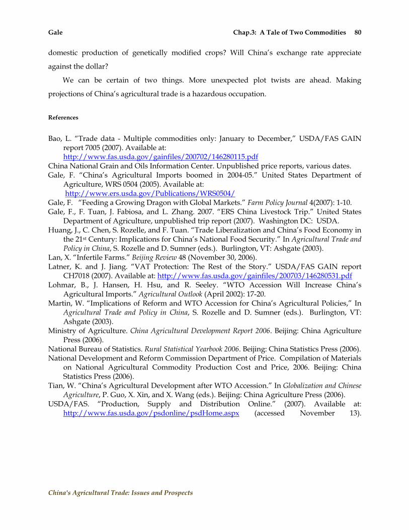
Gale Chap.3: A Tale of Two Commodities 80
China's Agricultural Trade: Issues and Prospects
domestic production of genetically modified crops? Will China‘s exchange rate appreciate
against the dollar?
We can be certain of two things. More unexpected plot twists are ahead. Making
projections of China‘s agricultural trade is a hazardous occupation.
References
Bao, L. ―Trade data - Multiple commodities only: January to December,‖ USDA/FAS GAIN
report 7005 (2007). Available at: http://www.fas.usda.gov/gainfiles/200702/146280115.pdf
China National Grain and Oils Information Center. Unpublished price reports, various dates. Gale, F. ―China‘s Agricultural Imports boomed in 2004-05.‖ United States Department of
Agriculture, WRS 0504 (2005). Available at: http://www.ers.usda.gov/Publications/WRS0504/
Gale, F. ―Feeding a Growing Dragon with Global Markets.‖ Farm Policy Journal 4(2007): 1-10. Gale, F., F. Tuan, J. Fabiosa, and L. Zhang. 2007. ―ERS China Livestock Trip.‖ United States
Department of Agriculture, unpublished trip report (2007). Washington DC: USDA. Huang, J., C. Chen, S. Rozelle, and F. Tuan. ―Trade Liberalization and China‘s Food Economy in
the 21st Century: Implications for China‘s National Food Security.‖ In Agricultural Trade and Policy in China, S. Rozelle and D. Sumner (eds.). Burlington, VT: Ashgate (2003).
Lan, X. ―Infertile Farms.‖ Beijing Review 48 (November 30, 2006). Latner, K. and J. Jiang. ―VAT Protection: The Rest of the Story.‖ USDA/FAS GAIN report
CH7018 (2007). Available at: http://www.fas.usda.gov/gainfiles/200703/146280531.pdf Lohmar, B., J. Hansen, H. Hsu, and R. Seeley. ―WTO Accession Will Increase China‘s
Agricultural Imports.‖ Agricultural Outlook (April 2002): 17-20. Martin, W. ―Implications of Reform and WTO Accession for China‘s Agricultural Policies,‖ In
Agricultural Trade and Policy in China, S. Rozelle and D. Sumner (eds.). Burlington, VT: Ashgate (2003).
Ministry of Agriculture. China Agricultural Development Report 2006. Beijing: China Agriculture Press (2006).
National Bureau of Statistics. Rural Statistical Yearbook 2006. Beijing: China Statistics Press (2006). National Development and Reform Commission Department of Price. Compilation of Materials
on National Agricultural Commodity Production Cost and Price, 2006. Beijing: China Statistics Press (2006).
Tian, W. ―China‘s Agricultural Development after WTO Accession.‖ In Globalization and Chinese Agriculture, P. Guo, X. Xin, and X. Wang (eds.). Beijing: China Agriculture Press (2006).
USDA/FAS. ―Production, Supply and Distribution Online.‖ (2007). Available at: http://www.fas.usda.gov/psdonline/psdHome.aspx (accessed November 13).
Cheng Chap.4: China’s Agriculture within the World Trading System 81
China's Agricultural Trade: Issues and Prospects
Chapter 4:
China’s Agriculture within the World Trading System
GUOQIANG CHENG
Institute of Market Economy Development Research Center of the State Council of China

Cheng Chap.4: China’s Agriculture within the World Trading System 82
China's Agricultural Trade: Issues and Prospects
China’s Agriculture within the World Trading System
Chapter 4:
Introduction
China is a large and developing country with a population of 1.3 billion, where agriculture has
been always considered a strategic industry that could stabilize the nation and pacify the
people. China‘s market-oriented rural reform, launched in 1978, has become a historical turning
point of its agricultural development. The reform broke the limitations of the traditional system,
accelerated rural economic development and accomplished the achievement of feeding nearly
21% of the world‘s population with less than 9% of the world‘s arable land. Moreover, rural
reform promoted overall reform of China‘s economic system and boosted fast growth of the
Chinese economy. Since its accession to the WTO, China has increased the openness of its
agricultural sector. There have been significant changes in the relationship between China‘s
agriculture and the world market. Within the world trading system, as a large producer and a
large consumer of agricultural products, China may be adversely affected by the international
market, but it may also exert a tremendous impact on the international market.
China’s Agriculture: Growth and Structural Changes
Agriculture and China’s Economic Growth: As a fundamental sector of its national
economy, China‘s agriculture has made a tremendous contribution to China‘s economic growth.
In 1978, China‘s agriculture accounted for 28.1% of GDP and provided 70.5% of the
employment opportunities (Figure 1). The reform initiated in that year greatly promoted
China‘s economic growth. China‘s GDP grew by an average annual rate of 9.7% in real terms
from 1978 to 2006. The growth of the agricultural sector (4.5%) was not as high as that of
industry (11.6%) and the service sector (10.3%) (NBSC), but as the foundation of the national
economy, its stable growth has sustained China‘s rapid economic growth and smooth
development during the reform and opening-up.
With rapid development of industrialization and urbanization, the Chinese economy has
experienced tremendous structural changes. The contribution of agriculture to the national
economy has been decreasing for many years (Table 1 and Figure 1). Up to 2006, the share of
agriculture in Chinese GDP dropped to 11.8% and the percentage of the workforce engaged in
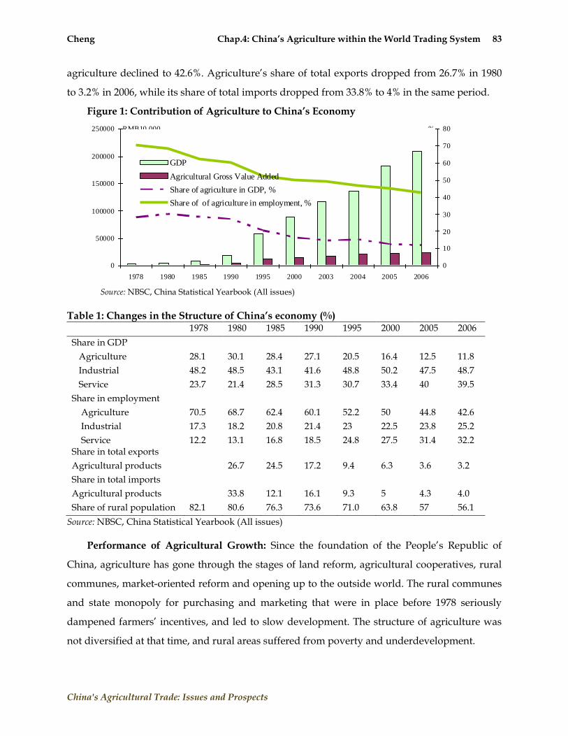
Cheng Chap.4: China’s Agriculture within the World Trading System 83
China's Agricultural Trade: Issues and Prospects
agriculture declined to 42.6%. Agriculture‘s share of total exports dropped from 26.7% in 1980
to 3.2% in 2006, while its share of total imports dropped from 33.8% to 4% in the same period.
Figure 1: Contribution of Agriculture to China’s Economy
0
50000
100000
150000
200000
250000
1978 1980 1985 1990 1995 2000 2003 2004 2005 2006
0
10
20
30
40
50
60
70
80
GDP
Agricultural Gross Value Added
Share of agriculture in GDP, %
Share of of agriculture in employment, %
%RMB10,000
Source: NBSC, China Statistical Yearbook (All issues)
Table 1: Changes in the Structure of China’s economy (%)
1978 1980 1985 1990 1995 2000 2005 2006
Share in GDP
Agriculture 28.1 30.1 28.4 27.1 20.5 16.4 12.5 11.8
Industrial 48.2 48.5 43.1 41.6 48.8 50.2 47.5 48.7
Service 23.7 21.4 28.5 31.3 30.7 33.4 40 39.5
Share in employment
Agriculture 70.5 68.7 62.4 60.1 52.2 50 44.8 42.6
Industrial 17.3 18.2 20.8 21.4 23 22.5 23.8 25.2
Service 12.2 13.1 16.8 18.5 24.8 27.5 31.4 32.2 Share in total exports
Agricultural products 26.7 24.5 17.2 9.4 6.3 3.6 3.2
Share in total imports
Agricultural products 33.8 12.1 16.1 9.3 5 4.3 4.0
Share of rural population 82.1 80.6 76.3 73.6 71.0 63.8 57 56.1
Source: NBSC, China Statistical Yearbook (All issues)
Performance of Agricultural Growth: Since the foundation of the People‘s Republic of
China, agriculture has gone through the stages of land reform, agricultural cooperatives, rural
communes, market-oriented reform and opening up to the outside world. The rural communes
and state monopoly for purchasing and marketing that were in place before 1978 seriously
dampened farmers‘ incentives, and led to slow development. The structure of agriculture was
not diversified at that time, and rural areas suffered from poverty and underdevelopment.
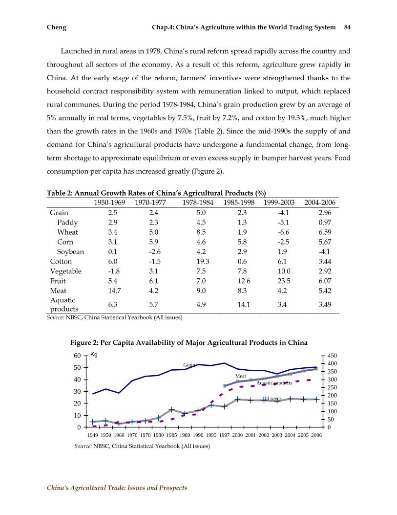
Cheng Chap.4: China’s Agriculture within the World Trading System 84
China's Agricultural Trade: Issues and Prospects
Launched in rural areas in 1978, China‘s rural reform spread rapidly across the country and
throughout all sectors of the economy. As a result of this reform, agriculture grew rapidly in
China. At the early stage of the reform, farmers‘ incentives were strengthened thanks to the
household contract responsibility system with remuneration linked to output, which replaced
rural communes. During the period 1978-1984, China‘s grain production grew by an average of
5% annually in real terms, vegetables by 7.5%, fruit by 7.2%, and cotton by 19.3%, much higher
than the growth rates in the 1960s and 1970s (Table 2). Since the mid-1990s the supply of and
demand for China‘s agricultural products have undergone a fundamental change, from long-
term shortage to approximate equilibrium or even excess supply in bumper harvest years. Food
consumption per capita has increased greatly (Figure 2).
Table 2: Annual Growth Rates of China’s Agricultural Products (%)
1950-1969 1970-1977 1978-1984 1985-1998 1999-2003 2004-2006
Grain 2.5 2.4 5.0 2.3 -4.1 2.96
Paddy 2.9 2.3 4.5 1.3 -5.1 0.97
Wheat 3.4 5.0 8.5 1.9 -6.6 6.59
Corn 3.1 5.9 4.6 5.8 -2.5 5.67
Soybean 0.1 -2.6 4.2 2.9 1.9 -4.1
Cotton 6.0 -1.5 19.3 0.6 6.1 3.44
Vegetable -1.8 3.1 7.5 7.8 10.0 2.92
Fruit 5.4 6.1 7.0 12.6 23.5 6.07
Meat 14.7 4.2 9.0 8.3 4.2 5.42
Aquatic products
6.3 5.7 4.9 14.1 3.4 3.49
Source: NBSC, China Statistical Yearbook (All issues)
Figure 2: Per Capita Availability of Major Agricultural Products in China
0
10
20
30
40
50
60
1949 1950 1960 1970 1978 1980 1985 1989 1990 1995 1997 2000 2001 2002 2003 2004 2005 2006
0
50
100
150
200
250
300
350
400
450
Grain
Meat
Aquatic products
Oil seeds
Kg
Source: NBSC, China Statistical Yearbook (All issues)

Cheng Chap.4: China’s Agriculture within the World Trading System 85
China's Agricultural Trade: Issues and Prospects
Since 1999, due to structural changes in the supply of and demand for agricultural
products, there has been a trend of low production of grain. The annual rate of reduction of
grain production reached 4.1% (Table 2). However, since 2004, the Chinese central government
has issued four key documents about supporting agriculture and rural development. These
documents have led to tremendous changes in agricultural production. For example, over the
period 2004 to 2006, grain production increased at the rate of 2.96% annually. Output of wheat
and corn also increased dramatically. Only soybean production decreased and rice production
remained unchanged.
So what are the causes of the growth of China‘s agriculture? Many studies have shown that
changes in agriculture since 1978 can be attributed to institutional innovations including the
household contract responsibility system with remuneration linked to output at the early stage
of the reform (Fan, 1991; Lin, 1992), as well as technological progress (Huang and Rozelle, 1996;
Fan and Pardey, 1997). Moreover, other factors also contributed to these changes such as
increased investment in agriculture, improved infrastructure for farmland, water conservancy
and irrigation facilities, market-oriented reform of agricultural product pricing and distribution
mechanisms and greater openness of the agricultural sector to the outside world.
Figure 3: Changes in the Structure (%) of China’s Agriculture
80
Crops, 50.8
15
Livestock, 32.2
1.6 Aquatic products, 10.4
3.4 Forestry, 3.8
0%
10%
20%
30%
40%
50%
60%
70%
80%
90%
100%
1978 1990 2000 2006
Source: NBSC, China Statistical Yearbook (All issues)
Structural Changes in the Agricultural Sector: Accompanying rapid development of the
agricultural sector, rapid growth of the national economy, urbanization and growth in
disposable income, there has been an increasing demand for meat products, aquatic products,
fruits and vegetables. The structure of agriculture has also undergone great changes. In terms of
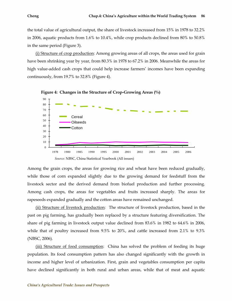
Cheng Chap.4: China’s Agriculture within the World Trading System 86
China's Agricultural Trade: Issues and Prospects
the total value of agricultural output, the share of livestock increased from 15% in 1978 to 32.2%
in 2006, aquatic products from 1.6% to 10.4%, while crop products declined from 80% to 50.8%
in the same period (Figure 3).
(i) Structure of crop production: Among growing areas of all crops, the areas used for grain
have been shrinking year by year, from 80.3% in 1978 to 67.2% in 2006. Meanwhile the areas for
high value-added cash crops that could help increase farmers‘ incomes have been expanding
continuously, from 19.7% to 32.8% (Figure 4).
Figure 4: Changes in the Structure of Crop-Growing Areas (%)
0
10
20
30
40
50
60
70
80
90
1978 1980 1985 1990 1995 2000 2001 2002 2003 2004 2005 2006
Cereal
Oilseeds
Cotton
Source: NBSC, China Statistical Yearbook (All issues)
Among the grain crops, the areas for growing rice and wheat have been reduced gradually,
while those of corn expanded slightly due to the growing demand for feedstuff from the
livestock sector and the derived demand from biofuel production and further processing.
Among cash crops, the areas for vegetables and fruits increased sharply. The areas for
rapeseeds expanded gradually and the cotton areas have remained unchanged.
(ii) Structure of livestock production: The structure of livestock production, based in the
past on pig farming, has gradually been replaced by a structure featuring diversification. The
share of pig farming in livestock output value declined from 83.6% in 1982 to 64.6% in 2006,
while that of poultry increased from 9.5% to 20%, and cattle increased from 2.1% to 9.3%
(NBSC, 2006).
(iii) Structure of food consumption: China has solved the problem of feeding its huge
population. Its food consumption pattern has also changed significantly with the growth in
income and higher level of urbanization. First, grain and vegetables consumption per capita
have declined significantly in both rural and urban areas, while that of meat and aquatic
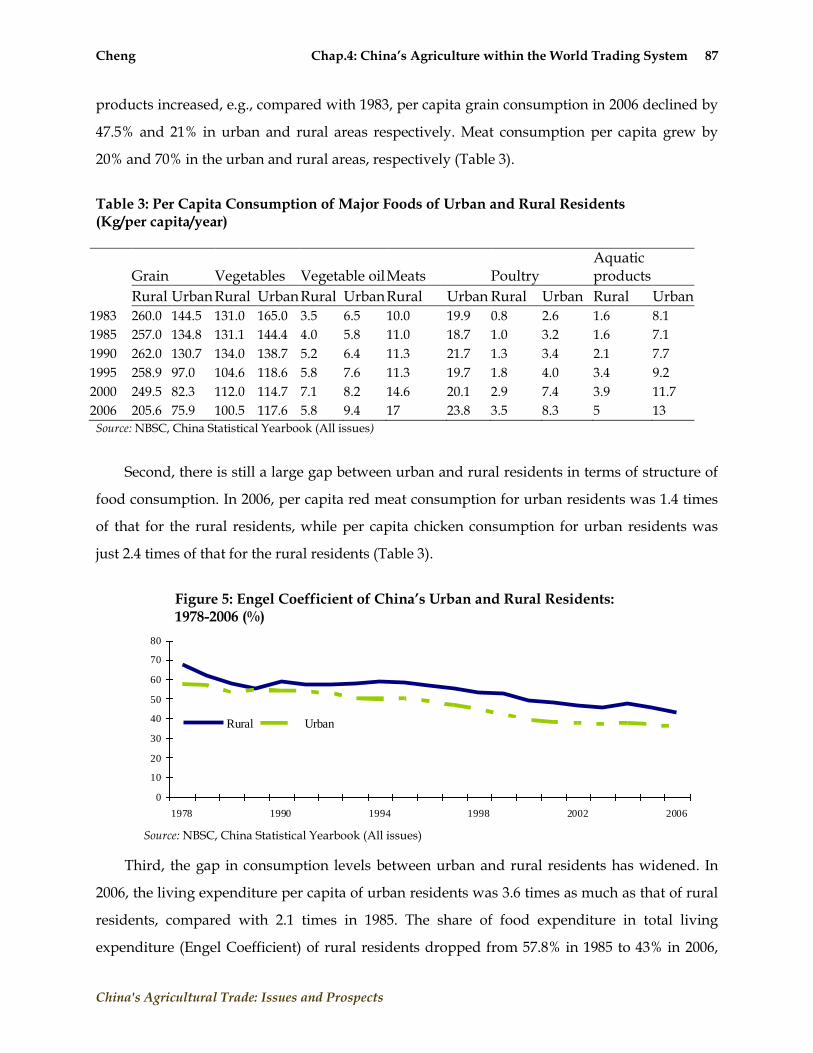
Cheng Chap.4: China’s Agriculture within the World Trading System 87
China's Agricultural Trade: Issues and Prospects
products increased, e.g., compared with 1983, per capita grain consumption in 2006 declined by
47.5% and 21% in urban and rural areas respectively. Meat consumption per capita grew by
20% and 70% in the urban and rural areas, respectively (Table 3).
Table 3: Per Capita Consumption of Major Foods of Urban and Rural Residents (Kg/per capita/year)
Grain Vegetables Vegetable oil Meats Poultry Aquatic products
Rural Urban Rural Urban Rural Urban Rural Urban Rural Urban Rural Urban
1983 260.0 144.5 131.0 165.0 3.5 6.5 10.0 19.9 0.8 2.6 1.6 8.1
1985 257.0 134.8 131.1 144.4 4.0 5.8 11.0 18.7 1.0 3.2 1.6 7.1
1990 262.0 130.7 134.0 138.7 5.2 6.4 11.3 21.7 1.3 3.4 2.1 7.7
1995 258.9 97.0 104.6 118.6 5.8 7.6 11.3 19.7 1.8 4.0 3.4 9.2
2000 249.5 82.3 112.0 114.7 7.1 8.2 14.6 20.1 2.9 7.4 3.9 11.7
2006 205.6 75.9 100.5 117.6 5.8 9.4 17 23.8 3.5 8.3 5 13
Source: NBSC, China Statistical Yearbook (All issues)
Second, there is still a large gap between urban and rural residents in terms of structure of
food consumption. In 2006, per capita red meat consumption for urban residents was 1.4 times
of that for the rural residents, while per capita chicken consumption for urban residents was
just 2.4 times of that for the rural residents (Table 3).
Figure 5: Engel Coefficient of China’s Urban and Rural Residents: 1978-2006 (%)
0
10
20
30
40
50
60
70
80
1978 1990 1994 1998 2002 2006
Rural Urban
Source: NBSC, China Statistical Yearbook (All issues)
Third, the gap in consumption levels between urban and rural residents has widened. In
2006, the living expenditure per capita of urban residents was 3.6 times as much as that of rural
residents, compared with 2.1 times in 1985. The share of food expenditure in total living
expenditure (Engel Coefficient) of rural residents dropped from 57.8% in 1985 to 43% in 2006,

Cheng Chap.4: China’s Agriculture within the World Trading System 88
China's Agricultural Trade: Issues and Prospects
and that of urban residents dropped from 53.3% to 35.8% (Figure 5). In 2006, food expenditure
per capita of urban residents was 3.7 times as much as that of rural residents, compared with 2
times in 1985 (NBSC, 2007).
China’s Agriculture and the World Trade System
Benefits from Global Economic Integration: China is now in the process of transition from
a planned economy toward a market-oriented economy, from a closed economy toward being
integrated with the global economy. China‘s agriculture has not only undergone rapid
development and significant restructuring, but also has gradually opened up to the outside
world and further integrated into the world trade system.
Table 4: China’s Agricultural Trade* - 1992-2006
Unit 1992 1995 2000 2001 2005 2006
Agricultural Gross Value Added (current value)
RMB billion
580 1199.3 1462.8 1541.2 2307 2470
Agricultural Gross Value Added (current value)**
USD billion
105.3 143.6 176.7 186.1 281.6 309.8
Agricultural exports USD billion
11.3 14.4 15.6 16.1 27.6 31.03
Agricultural imports USD billion
5.3 12.2 11.2 11.8 28.7 31.99
Ag Net Exports USD billion
6.0 2.2 4.4 4.3 -1.10 -0.96
Share in total trade
Share in total exports % 13.3 9.7 6.3 6.1 3.6 3.2
Share in total imports % 6.6 9.2 5.0 4.9 4.3 4.0
Ratio to AGVA
Exports % 10.8 10.0 8.8 8.7 9.8 10.0
Imports % 5.0 8.5 6.3 6.4 10.2 10.3
Imports and exports % 15.8 18.5 15.2 15.0 20.0 20.3
Source: China Customs Statistics from the General Administration of Customs; NBSC: China Statistical Yearbook (All issues) * Agricultural products in the table are defined by ―WTO definition + fishery‖, i.e., food + agricultural raw materials ** Calculated according to the official exchange rate of RMB against US dollar
With the fast development of China‘s foreign trade, China‘s trade in agricultural products
has also grown rapidly. Exports of agricultural products increased from less than US$11.3
billion in 1992 to US$31.03 billion in 2006, with an average annual growth rate of 7.5%. Imports
rose from US$5.3 billion to US$31.99 billion, with an average annual growth rate of 13.7% (Table
4). China has become the fifth largest agricultural exporter, after the US, EU, Canada and Brazil,

Cheng Chap.4: China’s Agriculture within the World Trading System 89
China's Agricultural Trade: Issues and Prospects
and the fourth largest agricultural importer, following the EU, US, and Japan. China now plays
a significant role in the world agricultural products market.
Despite rapid growth of China‘s trade in agricultural products, the share of agricultural
exports in total exports has shown a downward trend. The share of agricultural exports in total
exports declined from 13.3% in 1992 to 3.2% in 2006, while that of imports fell from 6.6% to 4%.
In some other countries, however, agricultural exports account for a significant portion in their
total trade volume. For example, the exports of agricultural products in New Zealand account
for 50% of its total of exports. For other countries, the share of agriculture in total exports is 20%
in Chile, 28% in Brail, 17.2% in Australia, 11% in Thailand, 7.2% in Canada, and 7.5% in the US.
The growth of trade in China‘s agricultural products indicates that participating in
international competition and sharing the benefits of global integration have played an
important role in China‘s economic development. First, agricultural exports still make great
contributions to China‘s foreign exchange reserves. From 1992 to 2003, China‘s cumulative
foreign trade surplus reached US$242.65 billion, and the cumulative net value of agricultural
exports reached US$51.33 billion, accounting for 21.2% of the total surplus, of which US$2.62
billion of the net value was achieved in 1992. This figure accounts for over 60% of the trade
surplus for the whole country. The net agricultural exports in 2003 reached US$2.35 billion,
9.2% of the total trade surplus. However, since 2004, China‘s agriculture began to witness a
trade deficit, ending the contribution of agricultural trade to foreign exchange reserves.
Second, agricultural exports play an important role in creating employment opportunities
for farmers, increasing their income, restructuring agriculture, and enhancing agricultural
competitiveness. Some studies have found that China‘s export multiplier of agricultural
products reached 1.66 in 2002, which means that US$1 of agricultural products exported could
create an additional US$1.66 worth of economic activities. Every US$10,000 of such exports can
directly and indirectly create nearly 28 jobs (Cheng, 2004a). Table 5 indicates that labor-
intensive agricultural products accounted for more than 76% of China‘s total agricultural
exports, and the share is still rising. This is significant in that it enables China to enjoy its
comparative advantage in agriculture and increase its agricultural competitiveness.
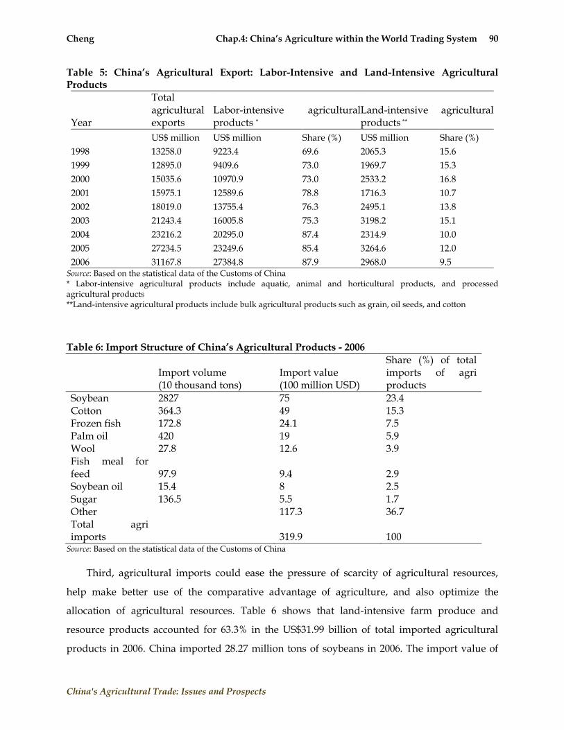
Cheng Chap.4: China’s Agriculture within the World Trading System 90
China's Agricultural Trade: Issues and Prospects
Table 5: China’s Agricultural Export: Labor-Intensive and Land-Intensive Agricultural Products
Year
Total agricultural exports
Labor-intensive agricultural products *
Land-intensive agricultural products **
US$ million US$ million Share (%) US$ million Share (%)
1998 13258.0 9223.4 69.6 2065.3 15.6
1999 12895.0 9409.6 73.0 1969.7 15.3
2000 15035.6 10970.9 73.0 2533.2 16.8
2001 15975.1 12589.6 78.8 1716.3 10.7
2002 18019.0 13755.4 76.3 2495.1 13.8
2003 21243.4 16005.8 75.3 3198.2 15.1
2004 23216.2 20295.0 87.4 2314.9 10.0
2005 27234.5 23249.6 85.4 3264.6 12.0
2006 31167.8 27384.8 87.9 2968.0 9.5 Source: Based on the statistical data of the Customs of China * Labor-intensive agricultural products include aquatic, animal and horticultural products, and processed agricultural products **Land-intensive agricultural products include bulk agricultural products such as grain, oil seeds, and cotton
Table 6: Import Structure of China’s Agricultural Products - 2006
Import volume (10 thousand tons)
Import value (100 million USD)
Share (%) of total imports of agri products
Soybean 2827 75 23.4 Cotton 364.3 49 15.3 Frozen fish 172.8 24.1 7.5 Palm oil 420 19 5.9 Wool 27.8 12.6 3.9 Fish meal for feed 97.9 9.4 2.9 Soybean oil 15.4 8 2.5 Sugar 136.5 5.5 1.7 Other 117.3 36.7 Total agri imports 319.9 100
Source: Based on the statistical data of the Customs of China
Third, agricultural imports could ease the pressure of scarcity of agricultural resources,
help make better use of the comparative advantage of agriculture, and also optimize the
allocation of agricultural resources. Table 6 shows that land-intensive farm produce and
resource products accounted for 63.3% in the US$31.99 billion of total imported agricultural
products in 2006. China imported 28.27 million tons of soybeans in 2006. The import value of

Cheng Chap.4: China’s Agriculture within the World Trading System 91
China's Agricultural Trade: Issues and Prospects
US$7.5 billion accounted for 23.4% of the total value of imported agricultural products. The
volume of imported soybean oil (15.5 million tons) is 1.8 times more than the domestic output.
This means that 80% of the demand for soybean oil has to be met by the imports. Cotton
imports reached 3.643 million tons, worth US$4.9 billion, accounting for 15.3% of total
agricultural imports. In addition to soybeans and cotton, China also imports resource products
such as frozen fish, palm oil, fish meal and wool.
Degree of Participation in the World Trade System: China‘s economy has integrated into
the world economy to a large extent. China not only benefits from globalization, but has also
become a driving force in world economic growth, from which other countries benefit. China
has become the largest destination of foreign direct investment. The degree of reliance of
China‘s economy on foreign trade has now reached 67%.1
The correlation of China‘s agriculture with the world market is increasing, the ratio of total
agricultural imports and exports to agricultural gross value added (AGVA) increasing from
15.8% in 1992 to 20.3% in 2006, which indicates deeper integration into the world trading
system. However, compared with China‘s economy as a whole, the degree of reliance of
agriculture on trade was not that high. The ratio of China‘s agricultural exports to its AGVA is
only 10%, whereas that of the U.S. is 41.1%, the EU 34% and Russia 36%.2,3 For some leading
exporters of agricultural products, such as Canada, Australia, Brazil and Thailand, the degree of
reliance on agricultural trade stood as high as 99%-175%, which means the agricultural sector of
these countries rely very heavily on the international market. Trade liberalization in
international agricultural products is of great importance to their agricultural development. It is
obvious that China‘s agricultural growth depends much more on domestic demand and
agricultural resources are mainly used in producing major agricultural products, such as grain,
for domestic consumption. In contrast, the degree of reliance on imports of agricultural
products relative to AGVA has increased gradually from 5% in 1992 to 10.03% in 2006. China
was the eighth largest importer of agricultural products in the early 1990s. Now it has become
the fourth largest importer of agricultural products following the EU, the US and Japan. China
is now the largest importer of soybeans, cotton, palm oil, wool, barley and sugar in the world.
1 Share of total trade value in GDP. 2 Due to the inclusion of forest gross value-added in the domestic AGVA, the degree of reliance of agriculture on trade is underestimated. The true degree is estimated to range from 10 to 20%. 3 Estimation based on ―World Development Index‖ of the World Bank (2006).
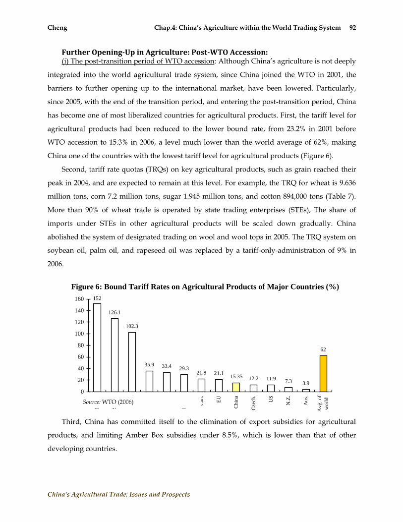
Cheng Chap.4: China’s Agriculture within the World Trading System 92
China's Agricultural Trade: Issues and Prospects
Further Opening-Up in Agriculture: Post-WTO Accession: (i) The post-transition period of WTO accession: Although China‘s agriculture is not deeply
integrated into the world agricultural trade system, since China joined the WTO in 2001, the
barriers to further opening up to the international market, have been lowered. Particularly,
since 2005, with the end of the transition period, and entering the post-transition period, China
has become one of most liberalized countries for agricultural products. First, the tariff level for
agricultural products had been reduced to the lower bound rate, from 23.2% in 2001 before
WTO accession to 15.3% in 2006, a level much lower than the world average of 62%, making
China one of the countries with the lowest tariff level for agricultural products (Figure 6).
Second, tariff rate quotas (TRQs) on key agricultural products, such as grain reached their
peak in 2004, and are expected to remain at this level. For example, the TRQ for wheat is 9.636
million tons, corn 7.2 million tons, sugar 1.945 million tons, and cotton 894,000 tons (Table 7).
More than 90% of wheat trade is operated by state trading enterprises (STEs), The share of
imports under STEs in other agricultural products will be scaled down gradually. China
abolished the system of designated trading on wool and wool tops in 2005. The TRQ system on
soybean oil, palm oil, and rapeseed oil was replaced by a tariff-only-administration of 9% in
2006.
Figure 6: Bound Tariff Rates on Agricultural Products of Major Countries (%)
152
126.1
102.3
35.9 33.4 29.321.8 21.1
15.35 12.2 11.97.3 3.9
62
0
20
40
60
80
100
120
140
160
No
rw.
Sw
itz.
Icel
.
Po
l.
Jap
an
Hu
ng
.
Can
.
EU
Ch
ina
Cze
ch.
US
N.Z
.
Au
s.
Av
g.
of
wo
rld
Third, China has committed itself to the elimination of export subsidies for agricultural
products, and limiting Amber Box subsidies under 8.5%, which is lower than that of other
developing countries.
Source: WTO (2006)

Cheng Chap.4: China’s Agriculture within the World Trading System 93
China's Agricultural Trade: Issues and Prospects
Table 7: China’s Tariff Rate Quotas on Agricultural Products - 2006
Quota (10,000 tons)
In-quota tariff rate (%)
STE share (%)
Non-STE share (%)
Out-of-quota tariff rate (%)
Wheat 963.6 1% 90% 10% 65
Corn 720 1-10% 60 40 65
Rice 532 1-9% 50 50 65
Sugar 194.5 15% 70 30 50
Cotton 89.4 1% 33 67 40
Wool 28.7 1% 38 Source: MOFCOM
(ii) Why limited impacts during the transition period of WTO accession? What puzzles
many observers is that bulk agricultural products, such as grain, where foreign countries have
an advantage, did not flood into China‘s market as expected. And the common concern that
China‘s agriculture would be seriously affected did not come true. We think there are several
reasons for this.
First, the Chinese Government has attached great importance to issues concerning
agriculture, rural areas and farmers. It has taken a series of more direct and effective policies
and measures in response to the situation since WTO accession. These favorable agricultural
policies and measures have promoted strategic restructuring of the rural economy, enhanced
agricultural competitiveness, and helped the sustained and steady growth of agriculture and
the rural economy.
Second, the impact of international competition on China‘s agriculture did not show up
initially due to the lagged effect of WTO accession.
Third, price fluctuations in domestic and international markets eased import pressure. For
example, the price for grain in the international market went up by 25-30% in 2002 because
major grain production countries had suffered serious problems. However, from 1997 to mid-
2003, China‘s domestic grain price had been low for seven consecutive years. Price conditions
were not favorable for the entry of grain from other countries. One additional thing needs to be
pointed out - in recent years, China‘s farmers have actually sacrificed their own economic
benefits in order to keep domestic grain prices at a low level, preventing the domestic market
from being affected by foreign competition.
(iii) Challenges in the post-transition period of WTO accession: Since the end of the
transition period, China‘s agriculture has entered a new phase of liberalization and it will
Cheng Chap.4: China’s Agriculture within the World Trading System 94
China's Agricultural Trade: Issues and Prospects
become integrated into the global economy. Some factors favorable to domestic agriculture will
disappear and some adverse factors are gradually emerging. The pressure of international
competition on China‘s agriculture will escalate. Particularly, China‘s traditional small-scale
agriculture, characterized by decentralized plantation, will not be able to compete with modern
foreign large-scale agriculture. The situation is unlikely to change for a long time. Also,
developed countries have given high subsidies and protection to their agriculture, which distort
the international trading environment. This unfavorable environment is also unlikely to change
in the near future. China‘s agriculture will face the effect and challenges of WTO accession for
some time, the impact and challenges emerging gradually after the transition period in terms of
five aspects.
First, the pressure of agricultural imports is increasing gradually. In recent years, there has
been a sharp increase in imports of soybeans and cotton. For example, soybean imports are 1.8
times more than domestic output. Cotton imports are four times more than the import quota.
The degree of reliance on cotton imports has reached over 40%. This has affected domestic
production and income growth to a large extent, causing much concern.
It is important to notice that the TRQs for grain imports have reached 22.16 million tons per
year, accounting for 15% of total grain output. According to Chinese statistics, if converted into
raw grain (including conversion of the soybean oil TRQ into equivalent amounts of soybeans),
the TRQs will stand at 41.07 million tons, equivalent to 8-9% of total domestic grain
consumption. This will have several key effects: grain imports will exceed the self-sufficiency
level set by the policy that 95% of grain should be domestically produced; the high level of
imports will pose a challenge to the control target of keeping a tightened balance of grain
supply and demand, and maintaining a high grain price. Grain imports will dampen domestic
prices, directly damaging the interests of grain-growing farmers and consequently influencing
the growth of grain output. Finally, it will affect the exercise of China‘s agriculture-supporting
policies, especially the current policy in favor of grain production.
Second, a trade deficit in agricultural products will become common in the future. In 2004,
it reached US$4.64 billion for the first time. China continued to witness a trade deficit in
agricultural products in 2005 through 2006. In light of the characteristics of supply and demand
for China‘s agricultural products and its natural endowments, it is preliminarily estimated that
China‘s reliance on agricultural imports will increase in the future. Agricultural trade will be

Cheng Chap.4: China’s Agriculture within the World Trading System 95
China's Agricultural Trade: Issues and Prospects
characterized by a large transactions volume (both imports and exports). A trade deficit will
likely become common, which could be a potential factor affecting the balance of payments.
Third, it will be more difficult to avoid and manage risks due to the international market.
With all industries open to the outside, China will face more and more risks and challenges
from international markets and it will be harder to avoid and reduce these risks, especially in
the agricultural products market. For example, at the end of April 2004, soybean prices in the
international market fluctuated drastically. The market risk immediately spread to China‘s
market through multinationals‘ marketing chains. As a result, the domestic soybean crushing
business suffered losses as high as RMB 5 billion.
Fourth, the environment for international agricultural product trade will become
increasingly complex. China will enter a period of frequent trade frictions. Technical barriers to
trade, anti-dumping rules, and specific safeguard mechanisms will become the major barriers to
China‘s agricultural exports.4 New barriers such as ―public opinion barriers‖ are also
emerging.5 Developed countries continue to provide subsidies to agriculture, which distort
international agricultural trade. The Doha Development Agenda that aims to establish new
rules of international trade, including trade in agriculture, is facing a dilemma. All these will
affect China‘s comparative advantage and expansion of agricultural exports in the coming
years.
In the near future, this will not only affect China‘s competitive advantage in increasing its
agricultural exports, but will also impose more pressure on China‘s domestic market for
agricultural products as a result of the likely steep increase in imports. In the context that the
rural population has not yet moved to urban areas in great numbers, this will bring about issues
of employment and income for a great number of farmers, which will intensify the nationwide
issues of economic reform, development and social stability in China.
Challenges and Key Problems in the Future
Since the late-1990s, China‘s agriculture has entered a new phase of development. The
interaction of supply and demand for agricultural products has undergone significant change,
4 According to the Protocol on China‘s Accession to the WTO, within 12 years of China‘s WTO entry, January 11, 2001 to December 11, 2013, when the products with China as the place of origin are exported to the territory of any WTO member, if the export volume increases sharply and thus causes ―serious damage‖ or ―serious damage threat‖ to related industries of the WTO members, the WTO members may separately take protection measures against the relevant Chinese products. 5 In recent years, some countries, including Japan, intentionally ―demonized‖ China‘s agricultural products through media such as newspapers and TV programs. This had a negative effect on China‘s agriculture and is therefore called a ―public opinion barrier‖.

Cheng Chap.4: China’s Agriculture within the World Trading System 96
China's Agricultural Trade: Issues and Prospects
achieving an historic transition from chronic shortage to approximate equilibrium or even
excess supply in bumper harvest years. With income growth, and significant changes in
consumption tastes and preferences, consumers demand agricultural products in greater
quantity and of higher quality. Agricultural development was constrained by resources in the
past and is now constrained by both resources and markets. Since WTO accession in 2001,
China‘s agriculture has become integrated into the global economy, where it faces competition
from home and abroad. Both the environment and conditions of China‘s agricultural
development have undergone profound and significant changes.
In the next few years, China will enter a new stage when its per capita GDP will increase
from US$1,000 to US$3,000, a stage characterized by accelerated industrialization, urbanization
and modernization. International experience indicates that it is not only a stage of strategic
opportunities, but also a stage of challenges and conflicts. In such a critical period, it is
important to solve the key issues concerning agriculture, rural areas and farmers and continue
to give play to the role of agriculture and the rural economy as a pillar for the national
economy. These issues not only have a bearing on increases in farmers‘ incomes, improvement
of agriculture efficiency and development of rural areas, but also have a direct impact on
China‘s grasp of strategic opportunities. They are of great significance for China‘s national
economy and social development. However, agriculture is still the weakest link in China‘s
national economy. A number of deep-seated problems restricting the development of
agriculture and the rural economy have not been fundamentally solved. In the foreseeable
future, China, as a major developing country, will face more and more pressure and challenges
in agriculture development. These pressures and challenges are as follows.
First, an increase in population and the resulting growth in demand for grain will place
great pressure on China‘s agriculture. China‘s population reached 1.314 billion by the end of
2006 and is expected to reach 1.345 billion by 2010. If calculated according to current grain
consumption patterns, demand for grain will be no less than 500 million tons by 2010. China‘s
grain production capacity is 470 million tons at present. It is quite difficult in terms of both
material conditions and technology to expand capacity to 500 million tons in 5 years. How to
ensure food security for a huge population will become an unavoidable strategic issue for
China‘s agriculture.

Cheng Chap.4: China’s Agriculture within the World Trading System 97
China's Agricultural Trade: Issues and Prospects
Second, the problem of rigid constraints on agricultural resources will become increasingly
prominent. The national situation in China is characterized by an enormous population with
insufficient arable land. Currently China‘s arable land per capita is less than 1.5 Mu (equivalent
to 0.1 hectare), amounting for only 43% of the world‘s average. The conflict between insufficient
arable land and the increasing population will exist for a long time. China‘s per capita
availability of water resources is only one fourth of the world‘s average. Drought and serious
water shortages have become bottlenecks to agricultural development in northwest, north and
central China. In the future, the problem of insufficient agricultural resources will become more
prominent and will directly threaten China‘s food security and agricultural products supply.
Third, it will be difficult for China to increase its agricultural competitiveness in the short
term. The gap between China and the major agricultural trading countries in terms of
technology, product quality and overall competitiveness will remain unchanged in the short
term. Also, China‘s inadequate agricultural investment, insufficient rural funds, continuous
outflow of production resources, and flawed marketing and service system for agriculture, as
well as an unsatisfactory agriculture-supporting policy will not change much for some time. It
is difficult for China to increase its agricultural competitiveness in the short term. Therefore,
China has to give full play to its advantages in global competition and choose a proper
development strategy.
Fourth, institutional problems limiting agricultural and rural development will begin to
emerge. In the context of accelerated urbanization and industrialization, some deep-seated
problems will develop in a society where there is a large gap between rural and urban areas.
For example, the gap between incomes, public services and social security will widen further
and there will be a sharp contrast in the outlook of urban and rural areas. Since the market for
input exchange between urban and rural areas has not been established, institutional barriers to
the transfer of the rural labor force will remain. It will be difficult to expand the channels for
increasing farmer‘s incomes and to create jobs for farmers. There is still a long way before
fundamental changes can be made to the stratified rural-urban structure that restricts
development of China‘s agriculture and rural areas.
Further Integrating into the World Trade System: Strategic Alternatives
It can be seen from the above analysis that in the world trade system, China is a large
developing country in terms of both population and agriculture; and it is facing far more

Cheng Chap.4: China’s Agriculture within the World Trading System 98
China's Agricultural Trade: Issues and Prospects
complex strategic problems than other countries. China‘s agriculture will continuously share
the enormous benefits of economic globalization and further integrate into the world trade
system. Meanwhile, China must also choose the correct development strategies, and take active
measures to meet various challenges from international competition.
Adhere to the Food Security Strategy of Relying Mainly on Domestic Supply: In order to
feed 21% of the world‘s population, China has always placed a high priority on promoting
grain production in terms of policy-making. Over the past few decades, the Chinese
government has never changed its food security strategy, characterized by solving the grain
issue mainly through domestic production. The strategy has also remained the same at the
various stages of agricultural development, either in the period of rural reform started in 1978,
or in the new phase of agricultural development since 1998 that has featured significant changes
in the supply and demand for agricultural products, and strategic restructuring of agriculture
and the rural economy. In the early 1990s, there were great concerns over China‘s ability to
support its population (Brown, 1995). The Chinese government issued a white paper on the
grain issue in 1996, and the debates on China‘s food security strategy have not ended.
Generally, questions over China‘s current food security strategy mainly come from the
perspectives of market efficiency or trade efficiency, which suggest that the strategy and related
policies are very costly. Various ideas have been proposed for improvement, including
liberalizing trade and making better use of the international grain market (World Bank, 1997;
2004), reducing the number of the grain varieties targeted by the food security policy, and a
transition from the commitment to ―food security‖ to ―rations security‖ only (CCICED, 2004).
We believe that China must adhere to the established food security strategy, i.e., meeting
demand for food based on domestic production and importing appropriate amounts of grain
from the international market.
The issue of food security in a country with huge population is complicated. Currently
China‘s grain production as well as consumption account for approximately 25% of the world‘s
total. The world‘s grain trade volume totals some 200 million tons, which represents only 40%
of China‘s grain consumption. If China‘s grain output declined by one percentage point, it
would have to import nearly 5 million tons to make up the shortage, which is 2.5% of the
world‘s grain trade volume. If China gave up its food security strategy based on domestic
production, it is difficult to forecast the implications for world trade in grain and the grain

Cheng Chap.4: China’s Agriculture within the World Trading System 99
China's Agricultural Trade: Issues and Prospects
market. Also, it is questionable whether China has enough purchasing power to guarantee the
supply of grain. Will China be able to bear the consequent adjustment and social cost? Will
other grain importers, especially those developing countries suffering from grain shortages, be
able to tolerate and adjust to the consequent changes in the world‘s grain supply-and-demand
relationship? We argue that food security in a country with a huge population is more than
simply an economic and trade issue. This helps one understand why China still gives high
policy priority to agriculture when it is doing its utmost to promote the market economy system
and further opening-up.6
The conditions for relying on grain trade in China have not been met yet. ―Based on
domestic production‖ does not indicate isolation from the global market. Since the 1980s, China
has been exploring ways to make better use of the international grain market. In the mid-1980s
and in the early and mid-1990s, the country imported grain in large quantities. In 2004, China
imported as much as 9.753 million tons of grain. However, putting aside the worries about
instability in the international grain market and other non-economic risks, technically speaking,
the country is basically not prepared to rely on the international market for grain. For example,
there are problems such as slow development of the domestic market, unsound grain markets,
underdeveloped trade associations, separate national markets and lack of risk management
mechanisms and tools.7 China has neither grain monopoly companies like those in the US,
France and Germany, nor trade organizations such as the Canadian and Australian Wheat
Boards, nor import administrative mechanisms such as those in Japan and South Korea.
Potential major players in the international market are still at the formative stages in China.
Besides, the country‘s current trading infrastructure is not capable of importing large quantities
of grain.
Should the rate of self-sufficiency of grain in China be adjusted? In the framework of the
WTO, the grain policy measures China could use are mainly concentrated on domestic
supports, consisting of non-trade distorting Green Box measures, such as promotion of research
and extension, development of agricultural infra-structure and non-production related direct
6 In the No.1 Document issued by the CPC Central Committee in 2004, the policy highlighted the importance of securing grain production while increasing farmers‘ income. The No.1 Document issued by the CPC Central Committee in 2005 expressly called for strengthening the overall agricultural (grain) production capacity. 7 For example: China lifted the embargo on imported soybeans as early as 1996. Due to lack of risk control experience and tools, fluctuating international market prices, and other factors, Chinese soybean businesses suffered combined losses of at least RMB 5 billion in 2004 (Cheng, 2004b).

Cheng Chap.4: China’s Agriculture within the World Trading System 100
China's Agricultural Trade: Issues and Prospects
subsidies as well as Amber Box measures, such as limited price support and input subsidies.8 In
terms of import controls, China has no other choice except TRQ administration. Therefore, the
so-called ―appropriate grain imports‖ essentially treats the committed grain TRQ as the bottom
line. As mentioned earlier, however, the grain TRQ is likely to surpass the target of a 95% self-
sufficiency rate.
Technically speaking, the coverage of food security policies should be analyzed in specific
contexts. That is to say that self-sufficiency rate targets differ from one category of grain to
another. For instance, China treats soybeans as one variety of grain, which differs from the grain
classification defined by international organizations such as the Food and Agriculture
Organization (FAO). Specifically, China liberalized soybean imports as early as in 1996 and
annual average imports over the past 7 years have reached 20 million tons, which means that
the self-sufficiency rate for soybeans was only 40%.9 If soybeans are included as one of the
grain-varieties, it is not helpful to overall judgment of the food security situation in China.
In this context, there are some possible policy suggestions. First, soybeans should be
excluded from the category of grains and should no longer be one of the grain varieties targeted
by the country‘s food security policy. Second, self-sufficiency rates should be based on specific
categories of grain. In principle, China has a comparative advantage and export potential in
rice, but due to high domestic demand and limited world supply, the country‘s rice production
should be targeted at maintaining the balance between domestic supply and demand. On the
other hand, China has less comparative advantage in wheat and corn production. If the wheat
and corn TRQs, 9.63 and 7.2 million tons respectively, are filled, the import volume will be
equivalent to 11% and 6% of domestic output respectively.10 Should self-sufficiency rate targets
for wheat and corn be adjusted accordingly? Third, further research should be conducted on
whether the scope of food security needs to be adjusted. For example, if ―rations security‖ is the
major concern, it is justifiable to liberalize corn imported as feedstuff, especially as it is a raw
material for biofuels production. However, ―rations security‖ does not reflect the existing
definition of ―food security‖. In major corn producing regions such as Jilin Province, corn is
directly related to increases in farmers‘ incomes, so without steady sources of income, the food
8 According to China‘s WTO entry commitments, the country may grant Amber Box subsidies that are equivalent to 8.5% of total agricultural output or of the output of a specific category of agricultural products. 9 Starting in 1996, soybean imports were subject to a single tariff rate of 3%. 10 According to the definitions of the WTO, a TRQ is an import opportunity that may not be used based on market conditions.

Cheng Chap.4: China’s Agriculture within the World Trading System 101
China's Agricultural Trade: Issues and Prospects
security of these farmers cannot be guaranteed. Under the circumstances that developed
countries grant high subsidies to corn producers and cross-border grain traders monopolize
global trading, what concerns many observers is that large quantities of corn imports could
change the current North-to-South Grain flow pattern. A likely pattern is that that North China
will not be able to export corn and South China will import corn in large quantities. The clear
losers will be farmers who live on corn production.
Develop an Agricultural Trade Strategy Promoting Further Integration of China’s
Agriculture into the World Trade System: It should be noted that promoting China‘s further
integration into the world trading system will place Chinese agriculture under more pressure
from international competition. At the same time, it will also help the country‘s agriculture
better enjoy the tremendous benefits brought by globalization. The key question is: what
strategy should China adopt for its agriculture to further integrate into the world trading
system? For quite a long time into the future, China‘s labor-intensive farm products such as
aquatic products, livestock, horticulture and processed products will have a substantial
comparative advantage in the world market. However, for land-intensive agricultural products
such as grain, cotton and oilseeds, it is the other way round. Obviously, under the pre-condition
of adhering to its food security strategy based mostly on domestic production, China should
adopt an agricultural trade strategy based on its comparative advantage. The essence of this
strategy includes the following.
First, improve the efficiency of resource allocation by promoting strategic restructuring of
agriculture. China has a huge population, and the per capita resource availability is relatively
low. Furthermore, with an increasing population, the problem of a relative shortage of
resources tends to become intensified. Implementing a strategy based on comparative
advantage could make best use of China‘s labor, expand the export of labor-intensive
agricultural products, facilitate the concentration of agricultural resources toward high-value
farm products, promote the strategic restructuring of agriculture, optimize the allocation of
resources and increase the overall productivity of China‘s agriculture. While adhering to the
national food security policy based on domestic production, an overall plan should be
developed in terms of the utilization of agricultural resources at home and abroad. An
appropriate amount of farm products should be imported, and a long-term strategic mechanism

Cheng Chap.4: China’s Agriculture within the World Trading System 102
China's Agricultural Trade: Issues and Prospects
that makes use of international resources as a supplement to China‘s serious shortage of land
and water resources should be established.
Second, releasing rural employment pressures should be a strategic starting point. China‘s
rural surplus labor stands at 120-200 million at present, and will be growing in the future. 11
Employment of farmers is the core difficulty in terms of the issues concerning agriculture, rural
areas and farmers. This requires a shift in China‘s export strategy of farm products, from
―contribution to foreign exchange‖ to ―contribution to employment‖. As far as China is
concerned, solving the issues of employment and incomes of the rural population will be more
significant in political terms than in economic terms for quite some time in the future – given
that China is at that stage of economic transition, where political interest in social stability is
more important than that of foreign exchange earnings. This will also reflect the idea of making
use of China‘s comparative advantage in labor-intensive farm products.
Third, increase China‘s agricultural competitiveness in the international market. One way
to enhance the international competitiveness of China‘s agriculture is to develop self-patented
know-how or introduce foreign technologies so as to improve the quality of products and their
technical intensification. While taking advantage of its comparative advantage characterized by
low labor costs, China must accelerate technical innovation and structural upgrading, deepen
the processing of agricultural products and optimize the trading structure of farm products
through introduction and development of new products. The combination of comparative
advantage based on labor-intensive production and core competence characterized by
technological innovation and structural upgrading would ensure the sustainable export growth
of China‘s agricultural products and dynamic comparative advantage.
Key Measures in the Near Future: Expand China‘s agricultural exports that have a
comparative advantage through several measures. First, a systematic plan to promote
agricultural exports should be made and greater support to agricultural exports should be
granted, so as to increase the competitive edge of China‘s agriculture in coping with the
increasingly complicated international trading environment and to offset the adverse effects of
unfair trade practices. Second, set up a multi-dimensional, orderly and effective system of
support and services for agricultural exports by combining product quality improvement with
penetration of technical barriers; encourage corporate entities to carry out technical upgrading
11 Research team under the Ministry of Agriculture of China: Research on the Issue of China‘s Rural Employment and Utilization of Surplus Labour in the Early 21st Century, Rural Economy in China, May 2000.

Cheng Chap.4: China’s Agriculture within the World Trading System 103
China's Agricultural Trade: Issues and Prospects
with branding strategies; combine comparative and late-comer advantages with the
establishment of core competence; combine a market diversification strategy with exploration of
key markets; combine export environment improvement with better export support and
services. Thirdly, take specific and effective strategic measures to tailor agricultural exports to
the international market
Take effective measures to prevent and offset the impact of sharp increases in agricultural
imports on the domestic market. These measures include, building a system to monitor
agricultural imports and give warning of industry damage and a subsequent response
mechanism, making full use of trade remedies such as anti-dumping measures, countervailing
and safeguard measures and developing an emergency mechanism to cope with high
agricultural subsidies in other countries.
Participate actively in the WTO Doha Round negotiations in an attempt to establish fair and
justifiable international trade rules. China should actively participate in the Doha Agricultural
Negotiations and play the role of a large developing country in order to make the result of the
negotiations more favorable to China. There are two things to be noted in particular. First,
China should demand that the developed countries reduce or even eliminate their domestic
agricultural subsidies and export subsidies. And most importantly, developed country
members should be prevented from utilizing the Doha Agricultural Negotiations to legalize
their agricultural protection policies in the framework of the WTO. Second, key agricultural
products such as grain, which are related to China‘s food security, rural employment and
farmers‘ incomes, should be included in the scope of special products for developing countries
that are exempt from reduction commitments, with a view to establishing a fair and justifiable
international economic environment for solving the issues concerning agriculture, rural areas
and farmers in China.
References Brown, L. R. Who Will Feed China? New York: W.W. Norton (1995). CCICED ―A New Framework for the Nation‘s Food Security Policy,‖ Policy Briefing (October
2004). Cheng, G. ―Chinese Agricultural Export: Growth, Structure and Contribution,‖ Management
World 10 (2004a). Cheng, G. ―Issues of the Development of China‘s Soybean Industry,‖ DRC Discussion Paper
(2004b).
Cheng Chap.4: China’s Agriculture within the World Trading System 104
China's Agricultural Trade: Issues and Prospects
Fan S. ―Effects of Technological Change and Institutional Reform on Production Growth in China‘s Agriculture,‖ American Journal of Agricultural Economics 73 (1991): 266-275.
Fan, S. and P. Pardey, 1997. ―Research Productivity and Output Growth in China‘s Agriculture,‖ Journal of Development Economics 53 (1997): 115-137.
General Administration of Customs, China Customs Statistics, issues from 1992 to 2006. Huang, J. and S. Rozelle. ―Technological Change: The Re- Discovery of the Engine of
Productivity Growth in China's Rice Economy,‖ Journal of Development Economics 49(1996): 337-369.
Lin, J.Y., 1992. ―Rural Reforms and Agricultural Growth in China,‖ American Economic Review 82 (1992): 34-51.
Ministry of Foreign Trade and Economic Cooperation. ―Compilation of the Legal Instruments on China's Accession to the World Trade Organization.‖ Beijing (2001).
National Bureau of Statistics of China. China Statistics Yearbook. Beijing: China Statistics Press, issues from 1985 to 2006.
World Bank. China in 2020. Washington DC: World Bank (1997). World Bank. ―China‘s Food Security,‖ Discussion Paper (2004). World Bank. World Development Indicators CD Rom. Washington DC: World Bank (2006). WTO. International Trade Statistics. Geneva: WTO (2006).

Huang et al. Chap.5: Measuring Distortions in China’s Agricultural Sector 105
China's Agricultural Trade: Issues and Prospects
Chapter 5:
Integrating China’s Agricultural Economy into the Global Market: Measuring Distortions in China’s Agricultural Sector
JIKUN HUANG1
YU LIU2
WILL MARTIN3 SCOTT ROZELLE4
1 Center for Chinese Agricultural Policy
2 China Center for Agricultural Policy 3The World Bank
4Stanford University

Huang et al. Chap.5: Measuring Distortions in China’s Agricultural Sector 106
China's Agricultural Trade: Issues and Prospects
Chapter 5:
Integrating China’s Agricultural Economy into the Global Market:
Measuring Distortions in China’s Agriculture Sector*
Introduction
Although there has long been an interest in the agricultural economy, it is quite surprising to
many that the agricultural sector of China actually has a record that is impressive in many
dimensions. Growth rates of gross domestic product, agricultural gross value added and food
per capita increased substantially between the early-1980s and the mid-2000s. Indeed,
agriculture‘s performance over the past two to three decades was more impressive than any
other country in South and Southeast Asia. Markets have boomed. The structure of agriculture
has fundamentally shifted. Despite having the largest population in the world and high income
growth (which has had a wrenching change on the nation‘s consumption bundle), since the
early-1980s China has been a net exporter of food in all but one year.
While the performance of the agricultural economy is well documented, there is less
understanding about the environment within which this growth occurred. In particular, there
have not been many studies of the external economy‘s environment that created some of the
incentives for producers. In the past, there has been work on the nature of the distortions to
China‘s agricultural economy, for example, Huang, Rozelle and Chang (2004), OECD (2005),
Orden et al. (2007). Unfortunately, these previous studies have only been partial. For example,
Huang et al. (2004) only looked at distortions in a single year; Orden et al. (2007) examined only
six years between 1995 and 2001. The OECD (2005) examined only a small set of commodities
and made a number of simplifying assumptions about some of the most important
commodities, such as pork meat and poultry. In part perhaps because of the partial nature of
these studies, they have come to a number of different conclusions.
*Acknowledgement: First published as Jikun Huang, Yu Liu, Will Martin and Scott Rozelle, 2007. ―Integrating
China‘s Agricultural Economy into the Global Market,‖ Ross Garnaut and Ligang Song (eds), China—Linking Markets for Growth, Asia Pacific Press, ANU E Press and Social Sciences Academic Press (China), The Australian National University, Canberra:118–132. The authors are grateful for helpful comments from workshop participants and for funding from World Bank Trust Funds provided by the governments of Ireland, Japan, the Netherlands (BNPP) and the United Kingdom (DfID), and Chinese Academy of Agricultural Sciences (KSCX2-YW-N-039).

Huang et al. Chap.5: Measuring Distortions in China’s Agricultural Sector 107
China's Agricultural Trade: Issues and Prospects
The purpose of this chapter is to examine the extent of China‘s agriculture integration into
the world market through estimations of indicators of direct and indirect interventions by
China‘s government in agriculture from 1981 to 2005. The main part of our analysis examines
the differences in prices between international prices and domestic wholesale prices at the
border, i.e., Nominal Rates of Assistance. We also consider distortions in the domestic economy
by examining the differences between farm-gate and border prices.
The wide scope of the goals and objectives, like other studies, also necessitate certain
limitations. First, the absence of data precludes us from examining the entire agricultural sector.
Instead, we examine commodities that account for nearly two-thirds of the gross value output
in all of the study years. Second, although we are able to judge from the price trends and an
understanding of domestic marketing and pricing, and trade policy reforms, the source of the
shifts in the distortions of the agricultural economy, we cannot identify the exact source of
changes. Also, although we use a revised exchange rate series in coming up with what we
believe are the correct values at which we convert international values into the domestic
currency, in a way that is useful in making any comparison with prices in China‘s domestic
economy, we do not analyze the effect of these assumptions. This is done elsewhere (Martin,
Huang and Rozelle, 2006).
The chapter is organized as the follows. In the next section, we discuss our quantitative
approach and sources of data. The results of the distortion analysis are presented in the third
section. The final section concludes.
Methodology and Data Sources
In this chapter, we have utilized the approach specified in Anderson, Martin, Sandri and
Valenzuela (2006). The approach is broadly based on comparisons between domestic and
international prices. During the reform era these price comparisons provide indicators of the
incentives for production, consumption and trade, and of the income transfers associated with
interventions.
Our approach essentially creates two measures of distortions for each major commodity in
the agricultural economy. The first measure in our analysis is the Nominal Rate of Assistance
(NRA). NRAs are used to compare the prices of commodities in the domestic economy (at the
port) with the international prices of commodities at the border (that is, cif at the port for
importable goods; fob at the port for exportable ones). Quality adjustments to the border prices

Huang et al. Chap.5: Measuring Distortions in China’s Agricultural Sector 108
China's Agricultural Trade: Issues and Prospects
have been made before we estimated NRAs. Conceptually, with NRAs we are trying to measure
the extent of distortions due to tariffs, exchange rate distortions, and other non-tariff barriers—
at the border.
Because of barriers within the domestic economy, the extent of protection (or dis-
protection) that is afforded by trade policies may not be the same as the real rate of protection to
farmers. Since we have independent observations on the prices obtained by farmers in local
markets we are able to estimate the nominal rate of assistance at the farm level taking into
account both border distortions and domestic distortions affecting farmer returns (NRAf‘s).
NRAf‗s are calculated after allowing for quality adjustment, tax or subsidies, transport, storage
and handling costs in moving commodities from the farm to the wholesale level. Differences
between NRAs and NRAf‘s arise from subsidy or transfer payments that cause the prices
received by farmers to differ from what they would receive under competitive internal market
conditions.
While NRAs (and NRAf‘s) only measure differences in output prices, there may also be
distortions on the input side. To capture these, it is possible to provide measures taking into
account direct subsidies and differences between the international prices of inputs and the
prices that farmers pay for these inputs. While these forms of protection (or taxation) are
important in many countries, and particularly in OECD countries, we find that they are
generally relatively small and so we focus on the NRA and NRAf measures when examining
distortions to producers.
Exchange rate distortions present particular measurement problems and require detailed
analysis if price-comparison-based measures are not to be misleading. The assumption and
methods that were used to generate our exchange rate series are in described in Appendix Table
A1. For documentation of our complete domestic and international price series, see Martin et al.
(2006).
In compiling our data we necessarily had to make choices on the coverage of the
commodities included in the study. Overall we have included 11 commodities: rice, wheat,
maize, soybeans, cotton, pork, milk, poultry, fruit (using apples as a representative product),
vegetables (using tomatoes as a representative product) and sugar (both sugar-beet and
sugarcane). Over the study period, these commodities accounted for between 75% (in the late-
1980s) and 60% (during the early-2000s) of the total value of agricultural output in China.

Huang et al. Chap.5: Measuring Distortions in China’s Agricultural Sector 109
China's Agricultural Trade: Issues and Prospects
Because decisions on production and consumption in China‘s domestic market were only
gradually being allowed to respond to domestic prices, and because we do not have access to
reliable data on the secondary market exchange rates prior to 1978, we focus on data for the
period beginning in 1980.
The data used in our study come from a number of sources, depending on the time period
of analysis and the commodity. Commodity balance data (production, utilization trade and
others) are from Center for Chinese Agricultural Policy‘s (CCAP) CAPSiM database, which are
mainly from the Ministry of Agriculture (production), National Bureau of Statistics of China
(NSBC) (consumption and others) and Ministry of Commerce (trade). Domestic prices are from
several different ministries. Specifically, farm-gate output prices come from the cost of
production surveys conducted by National Development and Reform Commission (NDRC).
Wholesale and retail prices of most products are from the Center for Price Monitoring, NDRC,
the Ministry of Agriculture (China Agricultural Development Report), and the Department of
Rural Survey under the NSBC. When wholesale and retail prices for some commodities in some
years are not available, price margins from farm-gate to wholesale and retail are estimated.
Much of the data on margins, transportation costs and other transaction costs are from an
extensive set of surveys by Huang and Rozelle during the 1990s and the early-2000s, surveys
which also served to establish which commodity price series provided appropriate bases for
price comparisons. Some of this was previously reported in Rozelle et al. (2000) and Huang et
al. (2004), which provided information on substantial quality differences between some
imported and domestic commodities and resulting biases in price comparisons as a measure of
protection. For more recent years, survey teams from the CCAP interviewed traders in 10 cities
around China in 2006. The complete data series are in the appendices of Huang et al. (2007).
The international price data (fob and cif) for all commodities except milk are the unit values
of exports or imports with adjustments for quality. These data are from the Ministry of
Commerce and China‘s Customs Administration. For the border price of milk, because no
import prices for milk are available, we use the farm gate price of milk in New Zealand adjusted
by international transportation and insurance rates to create a series for the international price
of milk (cif) that we refer to as the ―reference price.‖
Results

Huang et al. Chap.5: Measuring Distortions in China’s Agricultural Sector 110
China's Agricultural Trade: Issues and Prospects
The Role of Domestic Price and Marketing Policy: Before examining the role of
distortions at the border, it is useful to examine the relationship between the available domestic
price-series for farm and retail prices for the major grain crops (Table 1). The importance (and
role) of China‘s domestic price and marketing policy for rice and wheat (the three largest crops
in China) can be seen by comparing the state-set urban retail price and the state-set rural farm-
gate procurement price with the rural retail price (a free market price) before 1993 when the
urban grain rationing system was formally abolished. Until 1993, urban retail grain prices were
generally substantially below the price on the free market in rural areas, despite the costs
associated with transferring grain to urban areas. This was a consequence of a procurement
price system designed to provide urban residents with relatively inexpensive food. Only urban
residents could buy grain at these low prices and only with ration coupons that were available
in limited quantities.
Table 1: Rural Retail Price, Urban Retail Price and Farm-Gate Sales Price of Rice and Wheat in China, 1980-2005
1980-1993 1994-2001 2002-2005
Rice (in milled rice equivalent)
Farm-gate price 1375 1889 1939 Rural retail price 2069 2145 2112 Urban retail price 989 2144 2112
Wheat Farm-gate price 1126 1305 1268 Rural retail price 1700 1433 1325 Urban retail price 920 1433 1325
Sources: Computed by the authors based on various sources Note: the prices are yuan/ton in real 2005 yuan. Using the years of 1993 and 2001 as time division points because the former is the year of ending grain ration policy in urban area and the later is the year before China joined WTO
In addition, the marketing and procurement system may have been the source of additional
distortions. The relatively low selling price of grain at the farm-gate by farmers shows that
China‘s food system in the 1980s was set up to transfer income from rural to urban areas (Table
1, column 1). The amount that farmers received for mandatory deliveries was far below the free
market price. However, there is some question about the effects on incentives for production
and consumption given the infra-marginal nature of many of these transfers (Sicular, 1988). This
is because after the mid-1980s, farmers were able to sell additional amounts at higher market
prices once they had met their obligation to deliver a fixed quota quantity at the low purchasing

Huang et al. Chap.5: Measuring Distortions in China’s Agricultural Sector 111
China's Agricultural Trade: Issues and Prospects
price. If a farmer sold more grain than was required by his/her delivery quota, and the above
quota price was determined by market forces, there may have been less of a distortion.
Ultimately, however, even such policies are not fully decoupled from incentives, with
seemingly infra-marginal transfers away from rural households, for instance, giving their
members an incentive to move out of agriculture. These linkages have been shown by Wang,
Rozelle and Huang (1999). Therefore, the distortions created by domestic marketing and
procurement systems may have distorted incentives relative to international prices.
From 1994, however, changes to China‘s domestic marketing and procurement system
appear to have eliminated this additional layer of regulation for producers of rice and wheat
(Table 1, columns 2 and 3). In the early-1990s the urban price began to rise above the farm-gate
price; urban and rural retail prices also moved much closer together (Huang et al., 2007). This
reflects the phasing out of the implicit taxation of farmers through the grain procurement
system. The gap between urban and rural retail prices essentially disappeared after 1994 (Table
1). And the gap between the rural retail price and the farm price declined, possibly suggesting
an improvement in marketing efficiency (Park et al., 2002). With the disappearance of the
distortions from the marketing and procurement system, the remaining distortions after the
mid-1990s reflect only trade policies and not trade and domestic policies.
Nominal Rates of Assistance for China’s Main Agricultural Commodities: All NRAs and
NRAf‘s are computed at adjusted exchange rates (the estimated equilibrium exchange rates,
Appendix Table A1) since we believe this measure is the right one to use to calculate the true
rate of protection. In Martin et al. (2006) we report how the measures of distortions vary when
using official and adjusted exchange rates.
(i) Distortions to the grain economy before mid-1990s: The distortions to the rice economy
of China in the 1980s and early 1990s are characterized by two important features (Table 2, row
1). First, the NRA of rice, an exportable commodity, is negative between 1980 and 1993.
Averaging -23%, the negative NRAs show that China was highly competitive in international
rice markets during these years. Trade policy, however, kept exporters from shipping large
quantities of rice onto world markets and kept the free market price of rice in China‘s port cities
below the world price. Clearly this demonstrates China‘s commitment to keeping domestic
prices low. Even if there had been no other distortions in the rice economy, producers would
have faced prices below world market prices.

Huang et al. Chap.5: Measuring Distortions in China’s Agricultural Sector 112
China's Agricultural Trade: Issues and Prospects
The second feature demonstrates how domestic marketing and procurement placed a
greater tax on farmers and insulated the domestic price of rice from the world market price
even if trade policy had been liberalized (Table 2, rows 1 and 4). Because of China‘s marketing
policy that lasted through the mid-1990s, the state‘s artificially low procurement price kept the
price received by farmers systematically below the free market price of rice as seen by the
NRAf‘s. Because of this the tax on rice farmers averaged -42%. Rice producers were among the
most heavily taxed farmers in China—given the large share of the crop‘s sown area and large
negative rates of dis-protection. Importantly, our analysis shows how the state used trade and
procurement policy to tax its rice farmers.
Table 2: Nominal Rates of Assistance (NRA) and Nominal Rates of Assistance for Farmers (NRAf) in Cereal Sector in China, 1980-2005
1980-1993 1994-2001 2002-2005
NRA Rice -23 -4 -6 Wheat 47 25 0 Maize -1 7 16 NRAf Rice -42 -8 -9 Wheat 10 24 1 Maize -28 6 11 Source: Authors‘ estimates
Unlike rice, the NRA measures show that trade policy offered high rates of protection for
wheat farmers in China between 1980 and the mid-1990s (Table 2, rows 2 and 5). During the
period 1980-1993 the free market price of wheat in China‘s port cities was 47% higher than the
international price of wheat (cif, China‘s port cities). Unlike rice, which China produced
competitively during the 1980s, wheat producers—who have been shown to produce at a
higher cost than many other producers in other countries (Huang and Ma, 2000)—received
strong protection from trade policy. This policy on its own, unlike that for rice would not be
consistent with providing inexpensive food for consumers. It would, however, be consistent
with a policy of food self-sufficiency since it would encourage greater production by keeping
out imports and keeping domestic prices high.
Domestic marketing policies, however, were working in the opposite direction of trade
policies. The trends of the NRAf‘s show how the forced deliveries of wheat quotas insulated
farmers from the high rates of protection (Table 2, row 5). Although there was still positive
Huang et al. Chap.5: Measuring Distortions in China’s Agricultural Sector 113
China's Agricultural Trade: Issues and Prospects
protection for wheat farmers in most years between 1980 and 1994 the rates were lower
(averaging about 10%). These figures—along with those for rice—show that at least for China‘s
staple food crops, leaders were not trying to use prices to encourage food security.
The story of maize is a mix of those for rice and wheat (Table 2, rows 3 and 6). In
considering row 3, trade policy was providing very little protection for maize over the period
1980-1993, with an average of -1% for this period. Like the case of both rice and wheat,
procurement policy depressed the price of maize to China‘s farmers. Measured at farm-gate
level, maize farmers were taxed by 28% between 1980 and 1993.
(ii) Distortions to the grain economy after mid-1990s: After 1994, our distortions analysis
shows that China‘s international trade and domestic marketing policies have changed strikingly
(Table 2, columns 2 and 3). It is apparent from the way the differences in the estimates of NRAs
and NRAf‘s narrow that China‘s reformers were able to eliminate the procurement policies that
had been taxing rice, wheat and maize farmers (either by reducing the tax imposed by trade
policy as in the case of rice or reducing the protection as in the case of wheat). In other work,
Huang et al. (2006) show that the elimination of the procurement quota contributed
significantly to a reduction in the implicit tax burden shouldered by farmers.
The liberalization of domestic markets in the mid-1990s was accompanied by a
liberalization of trade policy, at least in the case of China‘s major food grains such as rice and
wheat. After the mid-1990s the taxation and subsidization of rice and wheat were clearly being
phased out as the NRAs for rice steadily rose (became less negative) and the NRAs for wheat
fell. Likely in part in preparation for its accession to the WTO, China‘s leaders liberalized trade
for its main food grains to such an extent that between 1995 and 2001 most of the protection for
the crops was eliminated. Since 2001, the NRAs for both rice and wheat have been almost zero.
Interestingly, the case of maize is a bit different than that for other crops (Table 2, row 3).
While NRAs moved towards zero in the case of maize, in a number of years after 2000, the NRA
for maize has been positive (not shown by the average figures in Table 2). This indicates that at
least in some years national leaders have been protecting maize producers. In part, as discussed
in Rozelle and Huang (2004), this may in part be due to the rise of the lobby from Jinin province
that has been successful in gaining protection for the producers of its most important crop.
(iii) Edible oils and cotton: The biggest difference between the analysis of distortions of
grain crops and for cash crops (at least for soybeans and cotton) is that domestic marketing

Huang et al. Chap.5: Measuring Distortions in China’s Agricultural Sector 114
China's Agricultural Trade: Issues and Prospects
policy has historically played less of a role. Although in some counties in China there was a
procurement delivery quota for soybean producers, it was not as widespread as that for grain
(in many counties soybeans were not procured by the state procurement system). In addition,
the implicit tax on soybeans in places in which soybean quotas were collected was lower than
that for the staple grain crops, there is little difference between the graphs for NRAs and NRAf‘s
(Huang et al., 2007). The same is true for cotton—except in the case of cotton through the mid-
1990s free market procurement of cotton by private traders was not allowed. When reform
finally came to the cotton industry in the mid-1990s, leaders did not move to a two-tier pricing
system, but instead allowed for both private trade and commercialized government cotton
procurement stations. As a result, the measures of distortion for the NRAs and NRAfs of cotton
are nearly the same (Huang et al., 2007). In fact, the same is true for all of the rest of the
commodities (livestock; horticulture and milk and sugar). As a result, the discussion in the rest
of this section—for all three periods—focuses on trade policy.
The trends in the NRAs after 1995 show the strong commitment to trade liberalization for
soybeans (Table 3, row 1). Beginning in the late 1990s and continuing through to 2005 the
protection for soybeans fell from around 25 to about 10%. This falling protection, in fact, should
not be a surprise given the integration of China into world soybean markets and the monotonic
rise in imports (which exceeded 25 million tons in 2005). The story of soybeans—and the fall in
protection and almost full liberalization—stands in sharp contrast to that of maize which
enjoyed increasing protection.
Table 3: Nominal Rates of Assistance for Farmers (NRAf) for Soybean, Cotton and Sugar-Crops in China, 1980-2005
1980-1993 1994-2001 2002-2005
Soybean na 24 12
Cotton -31 -6 -1
Sugar-crops 33 28 23 Source: Authors‘ estimates Note: The figures for sugar-crops are sugar output weighted average of sugarcane and sugar-beet
The distortion analysis for cotton, in some sense, produces results similar to those for rice
(Table 2, row 2). The combination of trade and monopoly procurement policies kept domestic
cotton prices lower than world market prices in the 1980s and early-1990s. Clearly it appears
that China‘s planners were taxing cotton farmers to supply its emerging textile industries with

Huang et al. Chap.5: Measuring Distortions in China’s Agricultural Sector 115
China's Agricultural Trade: Issues and Prospects
relatively inexpensive raw materials. It is no wonder with such high implicit taxes on cotton
that the lack interest by many suppliers (and serious insect problems) led to stagnant and even
falling area in many regions (NBSC, 2004).
After 1994, however, with the liberalization of domestic markets (mostly) and increased
trade liberalization (somewhat) there has clearly been a shift in the level of distortions faced by
cotton producers (Table 2, row 2). Although there were years in which there was fluctuation,
since the mid-1990s the NRAf has been gradually falling to nearly zero. In recent years, despite
the fact that national leaders could impose tariff rate quotas (TRQs) on cotton after a certain
amount is imported, in fact, trade officials essentially have left the level of imports in most years
to be determined by the market.
(iv)Livestock and horticultural commodities: With the exception of milk, the patterns of
distortions to China‘s livestock and horticultural sectors are quite similar (Table 4). In 1980-1993
there was heavy implicit taxation on pork and vegetables. In part, as noted by Huang et al.
(2004), this situation was created by China‘s grain-first policy. Although China can
competitively produce livestock and horticultural commodities, producers were neither
encouraged to produce or export these commodities on a large scale. Part of this was due to
China‘s own barriers, such as the quotas on exports into Hong Kong. Another part of the price
gap shown in these figures reflects trade barriers facing China in export markets. While there
quite possibly were grounds for some of the barriers (for example, foot and mouth disease is
widespread in China), even if a claim was blatantly false it could not be adjudicated effectively
since China was not part of WTO. As a consequence, China‘s livestock and horticultural
producers produced commodities far below the world market price and were neither inclined
nor able to increase exports into global markets.
Since the mid-1990s the gap between domestic and world prices of livestock producers has
fallen, but the trends are not clear for horticultural sector. Emerging markets and relaxation of
grain-first policies (often called agricultural structural adjustment policies inside China)
allowed producers to greatly expand livestock and horticultural production in large part to
meet the rising demand inside China (Rosen, Huang and Rozelle, 2004). At the same time
China‘s accession to the WTO and the appearance of an export-oriented segment of the
livestock and horticultural industries has increased the interest in and feasibility of participating
in international markets. In response, the price gap measures have been falling. It should be

Huang et al. Chap.5: Measuring Distortions in China’s Agricultural Sector 116
China's Agricultural Trade: Issues and Prospects
noted, however, that the NRAfs are all still negative. If anything, China‘s presence in global
food markets has given rise to more stringent rules and regulations on the import of livestock
and horticultural commodities from China.
Table 4: Nominal Rates of Assistance for Farmers (NRAf) in Livestock and Horticulture Sectors in China, 1980-2005
1980-1993 1994-2001 2002-2005
Milk 73 17 24 Poultry -11 -28 -19
Pork -57 -19 -8 Vegetable -50 -22 -23 Fruit -19 -29 -28
Source: Authors‘ estimates
(v) Milk and sugar: The story for milk and sugar is in some sense the opposite of that for
livestock and horticultural commodities. During the 1980s and early-1990s, the NRAfs for milk
and sugar were positive and large (Table 3, row 3 and Table 4, row 1). Those for milk averaged
70% in 1980-1993. Those for sugar were above 33% in the same period. After the mid-1990s,
protection has been lowered, and NRAfs for milk and sugar were falling (to around 20-25% for
the period 2002-2005).
Conclusions and Implications
The main finding of this chapter is that the nature of policy intervention in China‘s agriculture
has changed dramatically over the past 25 years, transforming the agricultural sector from one
characterized by high distortions to one that is relatively liberal and more integrated into the
world market. In the 1980s and early-1990s (or the early reform period) there were distortions in
both external and domestic policies that isolated domestic producers and consumers from
international markets. Importantly during the early reform period domestic marketing and
pricing policies actually served to make the prices that domestic producers and consumers
faced almost independent from the effects of trade policy. Because of this, even in the case of a
exportable commodity, e.g., rice, a commodity that enjoyed little protection at the border from
tariffs (meaning that the international price of rice and the free market price of rice were nearly
identical), domestic pricing and marketing policies did not allow producers to reap the profits
from international-level prices and instead forced farmers to sell much of their surplus to the
state at an artificially low price. Hence, domestic policies levied a tax on farmers even though
there was little protection at the border. Similar dynamics characterized importable

Huang et al. Chap.5: Measuring Distortions in China’s Agricultural Sector 117
China's Agricultural Trade: Issues and Prospects
commodities such as wheat and soybeans where, despite fairly high rates of protection from
trade policies, producers were receiving much less protection than they would have had there
been a free domestic market for the importable, while consumers were being implicitly taxed.
In contrast, since the early-1990s (the late reform period), liberalization of domestic markets
has reduced the distortions from domestic policies (as the market gradually has replaced the
state as the primary mechanism for allocating resources and has became the basis of farmer
production and marketing decisions). At the same time, especially in the case of importable
commodities, trade policy has become more liberalized, with distortions from border measures
falling substantially. As a result, we find that in recent years (that is, after China joined WTO at
the end of 2001) China‘s agriculture is much less distorted in two ways. First, the differences
between international and domestic market prices have narrowed considerably for many
commodities due to trade policy liberalization. Second, the elimination of domestic policy
distortions mean that when trade liberalization allows for the increased import or export of
agricultural commodities, prices in China‘s domestic market change and farmers are directly
affected by them.
Despite the finding that considerable liberalization has occurred due to policy reforms in
both domestic and external policies, there are still distortions to agriculture in the mid-2000s, 25
years after the beginning of reforms. In some cases, these remaining distortions arise from
tariffs on importable commodities and non-tariff trade barriers of other countries on China‘s
exportable commodities. While low by international comparisons, China is still providing a
degree of protection for a number of importable commodities, e.g., maize, sugar and milk.
With this analysis, we have shown that China‘s agriculture economy has become one of the
least distorted in the world. Clearly, the combination of domestic marketing reforms and
international trade liberalization has greatly freed up the decision making environment for
producers. In such an environment phenomena such as rapid structural change from grain to
more labor intensive commodities and the rise of a horticulture and livestock-based export
economy become more understandable. When farmers face less distortion they tend to move
into those commodities in which they have a comparative advantage.

Huang et al. Chap.5: Measuring Distortions in China’s Agricultural Sector 118
China's Agricultural Trade: Issues and Prospects
References
Anderson, K., W. Martin, D. Sandri, and E. Valenzuela. ―Methodology for Measuring
Distortions to Agricultural Incentives.‖ Working Paper, Development Research Group (2006). Washington DC: World Bank.
Huang, J., Y. Liu, W. Martin, and S. Rozelle. ―Distortions to Agricultural Incentives in China, 1981 to 2005.‖ Working Paper (2007). Washington DC: World Bank.
Huang, J. and H. Ma. ―International Comparison of Agricultural Prices.‖ International Trade 10(2000):20-24.
Huang, J., S. Rozelle, and M. Chang. ―The Nature of Distortions to Agricultural Incentives in China and Implications of WTO Accession.‖ World Bank Economic Review 18(2004): 59-84.
Huang, J., S. Rozelle, and H. Wang. ―Fostering or Stripping Rural China: Modernizing Agriculture and Rural to Urban Capital Flows.‖ The Developing Economies XLIV(2006): 1-26
Martin, W., J. Huang, and S. Rozelle. ―Exchange Rates and Agricultural Distortions in China‘s Agriculture, 1981 to 2004.‖ Working Paper (2006). Washington, DC: World Bank.
Ministry of Agriculture. China’s Agricultural Yearbook, various issues. Beijing: China Agricultural Press.
Ministry of Agriculture. China Agricultural Development Report. Beijing: China Agricultural Press.
Ministry of Commerce. China Foreign Trade Yearbook, various issues. Beijing: China Foreign Economic and Trade Press.
National Development and Reform Commission, Price Department. Agricultural Production Cost and Revenue Materials Compilation, various issues. Beijing: China Statistical Press.
National Development and Reform Commission, Center for Price Monitoring. National Major Commodity (Service) Price Monitoring Data Compilation. Unpublished, Beijing: NDRC.
NBSC (National Bureau of Statistics of China). Statistical Yearbook of China, various issues from 1981 to 2006. Beijing: China Statistical Press.
NBSC (National Bureau of Statistics of China). China Yearbook of Agricultural Price Survey, various issues. Beijing: China Statistical Press.
OECD. OECD PSE/CSE database. OECD. OECD Review of Agricultural Policies: China. Paris: OECD (2005). Office of Tariff Regulation, the State Council. Import and Export Tariff Regulation of the People's
Republic of China, 1996, 1997 and 1998. Beijing: Law Press. Office of Tariff Regulation, the State Council. Import Tariff and Export Tariff Rebate Compilation.
Beijing: Economic and Scientific Press (2005). Orden, D., F. Cheng, H. Nguyen, U. Grote, M. Thomas, K. Mullen and D. Sun. ―Agricultural
Producer Support Estimates for Developing Countries: Measurement Issues and Evidence from India, Indonesia, China, and Vietnam.‖ Research Report No. 152 (2007). Washington DC: International Food Policy Research Institute.
Park, A., H. Jin, S. Rozelle, and J, Huang. ―Market Emergence and Transition: Arbitrage, Transition Costs, and Autarky in China‘s Grain Market.‖ American Journal of Agricultural Economics 84 (2002):67-82.
Rosen, D., J. Huang, and S. Rozelle. ―Roots of Competitiveness: China‘s Evolving Agriculture Interests.‖ Policy Analysis in International Economics, 72 (2004). Washington DC: Institute for International Economics.

Huang et al. Chap.5: Measuring Distortions in China’s Agricultural Sector 119
China's Agricultural Trade: Issues and Prospects
Rozelle, S. and J. Huang. ―China‘s Maize Economy: Supply, Demand and Trade.‖ Report for the US Grains Council (2004). Beijing.
Rozelle, S. and J. Huang. ―China‘s Soybean Economy: Supply, Demand and Trade.‖ Report for the American Soybean Association (2005). Beijing.
Rozelle, S., A. Park, J. Huang, and H. Jin. ―Bureaucrat to Entrepreneur: The Changing Role of the State in China‘s Transitional Commodity Economy.‖ Economic Development and Cultural Change 48(2000): 227-252.
Sicular, T. ―Plan and Market in China‘s Agricultural Commerce.‖ Journal of Political Economy 96 (1988): 283-307.
Wang, D., Scott Rozelle, and J. Huang. ―The Impact of Procurement Quota on Agricultural Production in China‘s Agriculture,‖ Working Paper (1999). Beijing: Center for Chinese Agricultural Policy, Chinese Academy of Agricultural Sciences.

Huang et al. Chap.5: Measuring Distortions in China’s Agricultural Sector 120
China's Agricultural Trade: Issues and Prospects
Appendix Table A1: Raw Numbers for Exchange Rate Analysis, China, 1980-2005
Year Official
ratea
Secondary market
rateb
Retention ratec
Discount to secondary
market rate
Estimated equilibrium
exchange rated
1980 1.50 1.95 0.20 1.95 1.95
1981 1.71 2.05 0.20 2.05 2.80
1982 1.89 2.27 0.20 2.27 2.80
1983 1.98 2.39 0.20 2.39 2.80
1984 2.33 2.69 0.20 2.69 2.80
1985 2.94 3.05 0.25 3.05 2.95
1986 3.45 4.03 0.25 4.03 3.81
1987 3.72 4.40 0.44 4.40 5.29
1988 3.72 6.50 0.44 6.50 5.79
1989 3.77 6.60 0.44 6.60 4.94
1990 4.78 6.60 0.44 6.60 5.44
1991 5.32 6.60 0.80 6.60 5.84
1992 5.52 6.92 0.80 6.92 7.12
1993 5.76 8.28 0.80 8.28 8.41
1994 8.62 8.70 0.80 8.70 8.69
1995 8.35 n. a. n. a. n. a. 8.35
1996 8.31 n. a. n. a. n. a. 8.31
1997 8.29 n. a. n. a. n. a. 8.29
1998 8.28 n. a. n. a. n. a. 8.28
1999 8.28 n. a. n. a. n. a. 8.28
2000 8.28 n. a. n. a. n. a. 8.28
2001 8.28 n. a. n. a. n. a. 8.28
2002 8.28 n. a. n. a. n. a. 8.28
2003 8.28 n. a. n. a. n. a. 8.28
2004 8.28 n. a. n. a. n. a. 8.28
2005 8.19 n. a. n. a. n. a. 8.19
Notes: a NBSC; b Huang and David (1995); c The proportion of foreign currency actually sold by all exporters at the parallel market rate; d see Anderson et al. (2006) on the exchange rate methodology and Huang et al. (2007)

Zhong et al. Chap.6: Resource Mobility and Agricultural Trade Policy 121
China's Agricultural Trade: Issues and Prospects
Chapter 6:
Resource Mobility and China’s Agricultural Trade Policy
FUNING ZHONG1 JING ZHU1
ZHENGQIN XIE2
1 Nanjing Agricultural University 2 Nanjing University of Finance and Economics

Zhong et al. Chap.6: Resource Mobility and Agricultural Trade Policy 122
China's Agricultural Trade: Issues and Prospects
Chapter 6:
Resource Mobility and China’s Agricultural Trade Policy
Introduction
Agricultural trade policy in China has been under re-assessment since China‘s accession to the
WTO. Over the past decades, China has protected part of its agricultural sector through various
policy instruments. Production support and border measures have been successful in
promoting domestic agricultural production and protecting some producers from foreign
competitors. However, such results have been achieved at the price of inefficient resource
allocation and loss of trade benefits for the overall economy. After China joined the WTO, the
question of whether the same set of trade policies should be carried out has been under heated
discussion. Analysis from the point of view of comparative advantage and the benefits of free
trade suggests a more open trade policy and increasing government support toward labor-
intensive agricultural products (Huang et al., 2005; Zhong, 2003); whereas concerns from the
view of food security and the future growth of agricultural production lead to a preference for
policies towards strong protection, especially for land-intensive agricultural products such as
grain.
In this chapter we attempt to provide analysis from another important perspective:
resource mobility in agricultural production, and to argue that protection for sectors with low
resource mobility is needed during a period of transition. At the same time, greater effort needs
to be made to improve the mobility of these resources, which will lead to less trade protection in
the future and more gains from trade.
Resource mobility is one of the important assumptions of trade theory. In the Ricardian and
Heckscher–Ohlin models, free trade between two nations is always believed to bring mutual
benefit to both parties, because it leads to specialization of production and more efficient
resource allocation. Therefore, both nations‘ welfare will increase after an exchange of goods
produced at lower costs. However, if some factors of production are assumed to be tied to a
particular industry and are immobile, resources in the import-competing industry that cannot
move will receive lower rates of return, as depicted in the specific-factor model.

Zhong et al. Chap.6: Resource Mobility and Agricultural Trade Policy 123
China's Agricultural Trade: Issues and Prospects
Agricultural production resources are less mobile compared to other industries. Relocation
of resources may result in heavy losses, and there are long time-lags. High transaction costs
may inhibit the transfer of welfare. Under such circumstances, the economic and social impacts
of welfare changes, which result from freer trade, cannot be neglected. Support for protection is
grounded in the time period required for structural adjustment.
The specific-factors model provides a very important and useful analytical framework for
understanding the contradictions between conventional trade theory and practice. It has also
been applied in many empirical research studies (Burgon, 2001; Brecher and Choudhri, 1994;
Cassing and Ochs, 1978). However, the structure of the model as well as its application usually
reflects the situation in developed countries, in particular the industrial sector, which is
substantially different from the situation in the agricultural sector in developing countries such
as China.
The specific-factors model contains three factors of production: labor, capital, and land.
Labor is assumed to be a homogenous and mobile resource that can be used in either of two
sectors, manufacturing and food production, whereas capital is assumed to be low in mobility.
Labor is assumed to be mobile mainly because the time it takes labor to move between
geographic locations is limited. One influential study found that when a US state hits economic
difficulties, workers quickly begin leaving for other states, and within 6 years the
unemployment rate falls back to the national average (Blanchard and Katz, 1992). Labor is
generally classified as homogenous and can transfer from one sector to another. It is further
assumed that workers who have received highly specific training (a minority of the labor force)
are less mobile as compared to workers who have general skills (a majority of the labor force).
Capital is assumed to be low in mobility because it is hard to change the use of large machinery
equipment and even buildings: a lifetime of 15–20 years for a typical specialized machine and
50 years for office buildings are commonplace.
The situation is substantially different in the agricultural sector of developing countries:
capital is more mobile than labor. There are few large-scale machines or production-specific
capital investments. Capital investments for agricultural production are usually small, with
production tools or equipment used for one kind of crop production applicable for other kinds
of crop production as well. Labor movement, in contrast, is constrained by institutional,
cultural, educational, ethical, traditional and other constraints, both in the case of intra-sector

Zhong et al. Chap.6: Resource Mobility and Agricultural Trade Policy 124
China's Agricultural Trade: Issues and Prospects
and inter-sector movement (Cai, 2005). Moreover, labor is not homogeneous and cannot
transfer from the food to manufacturing sector as easily as in the case described in the specific-
factors model. On the contrary, due to the lower level of education in rural areas, only a small
group of farmers who are either better educated or trained are relatively mobile while the
majority, having received a low level of education and training, are relatively immobile (Zhao,
1997).
There is another important difference between the agricultural sector of developed
countries and that of developing countries, which deserves attention in policy discussions. In
developed countries, the owners of land, capital and labor used in agricultural production, are
usually not the same group of people. The immobility of one of two production resources (in
the specific-factors model, the sector-specific physical assets), may hurt only that specific group
of owners if an outside shock occurs. By contrast, in developing countries farmers are usually
both the labor and capital supplier to their own land, that is, they are the owner of, and all of
their profit comes from the return to, all three factors – land, labor and capital – in agricultural
production. Therefore, farmers are more vulnerable and may be hurt in multifaceted ways by
shocks in agricultural production. Compared to producers in developed countries, farmers in
developing countries are not only a much larger group, but also are far more vulnerable
because of their much lower and volatile income, and hence deserve more attention in policy
analysis. It is, therefore, necessary to carry out further research that better reflects the situation
and experience of the agricultural sector of developing countries. This chapter takes a
preliminary step towards analyzing resource mobility in Chinese agriculture production, the
constraints to mobility, and its implications for trade policies. The basic objective is to identify
the rationale of protection in the short run and to establish alternative measures to improve
resource mobility in the long run. Such measures aim to improve the welfare of farmers in
China who face heavy pressures from free trade and globalization.
Resource Mobility in Chinese Agriculture
Various production resources are required in the agricultural sector: (1) natural resources such
as land, climate, soil, and water; (2) capital inputs, such as machinery, seed, and fertilizer; (3)
human resources, including the quantity and quality of agricultural labor; and (4) institutional
arrangements such as government interventions in infrastructure that facilitate agricultural
Zhong et al. Chap.6: Resource Mobility and Agricultural Trade Policy 125
China's Agricultural Trade: Issues and Prospects
production and marketing. Because of different constraints and barriers to movement, the
mobility of these production resources varies widely across regions and production lines.
Natural Resources: Land is the most important resource in agricultural production. Unlike
other industries, agricultural production, especially crop production, cannot be carried out
without land. Land is physically fixed, and it is incapable of moving among regions. As a result,
the productivity of land for a particular crop is subject to specific climate, topography, soil and
water conditions attached to the location. Furthermore, as a productive input, land is also fixed
in a time dimension, and is incapable of moving among seasons. Farmers have to grow different
crops during different seasons in a year, or rotate different crops in sequence if they want to
maximize returns. In this sense, even if one type of agricultural production enjoys comparative
advantage and has good prospects for export expansion, a farmer cannot expand this
production significantly without acquiring additional land. If the comparative advantage is
attached to a specific location, then farmers in this area may not be able to expand their
production as a whole. Although technological innovation would help to improve land
productivity to a certain extent, the output would still be constrained by land limitations,
especially in the short run and without significant increases in costs.
In a populous developing country such as China, where even marginal land has been
cultivated, any expansion of farm produce with comparative advantage to meet export demand
cannot be done by cultivating new land. Rather, it can only be realized by shifting certain
cultivated land from its existing usage. However, a climate favorable to production of one crop
or animal cannot be extended to other places, so the expansion of agricultural production to
cover larger areas and/or other locations may not enjoy the same comparative advantage, at
least not to the same extent. Therefore, a certain combination of land, soil and climatic
characteristics determine whether a region is favorable to producing certain agricultural
products, and is producing at a lower cost with comparative advantage. Even if the same
products can be produced in other regions, they can hardly be produced at a comparable cost
due to the difference in other natural conditions.
China is vast in land and diverse in natural conditions in different regions. Therefore, each
region produces products that best reflect its natural endowment. In this study, we separate the
country into six agricultural regions according to natural conditions and the resultant pattern of
agricultural production. Each region, because of its natural endowment, is favorable to

Zhong et al. Chap.6: Resource Mobility and Agricultural Trade Policy 126
China's Agricultural Trade: Issues and Prospects
producing certain kinds of agricultural production in comparison with other regions of the
country.
Region 1 is the Northwest Region, which includes Inner Mongolia, Ningxia, Gansu,
Qinghai, Xinjiang and Tibet. Production of sheep wool is concentrated in this region, accounting
for 60% of the national total, and that of beetroot has increased from 20 to 80% of the national
total in less than 30 years. Region 2 is the Northeast Region consisting of Heilongjiang, Jilin and
Liaoning. This region is a major producer of grain crops with 40 to 50% of the country‘s
soybeans and 30% of the country‘s corn being produced in this region. Region 3 is the North
Region, including Beijing, Tianjin, Hebei, Henan, Shandong, Shanxi and Shaanxi. Wheat
production in this region is more than 60%of the national total, with cotton production ranging
from 30 to 60% of the national total. Rapeseed production is concentrated in this region,
involving 25 to 45% of sown area, while production of silkworm cocoons amounts to more than
20% of the national total. Region 5 is the Southeast Region, which includes Zhejiang, Shanghai,
Fujian, Jiangxi, Hunan, Guangdong, Guangxi and Hainan. In addition to rice, tropical crops
dominate in this region, with around 80% of sugar cane and 50% of rice in China being
produced in this region. Region 6 is the Southwestern region, which includes Sichuan,
Chongqing, Yunnan and Guizhou. The production of tobacco in this region, measured in share
of sown areas, is more than double that of the country in past decades. At the same time, pig
meat production in this region accounts for more than 20% of the national total.
From the above description we may conclude that, because of the constraints of natural
resources in climate, topography, water, and soil condition, agricultural production in different
parts of China varies to a great extent. Table 1 is a summary of major agricultural products in
the six regions and their output relative to the national total. It can be seen from the table that in
each region there are some agricultural products with high levels of production. The differences
in natural conditions and the immobility of land resources lead to production concentrations
located in different parts of the country, making it difficult to transfer other production
resources among products, other than land itself.
Capital: In economic theory, capital is usually treated as investment in fixed assets that
may be used in production for a long time. It provides more or less the same service during its
lifespan, while its value is gradually transferred to products over time. However, in many
theoretical and empirical studies, capital is also treated as a production resource, and is then
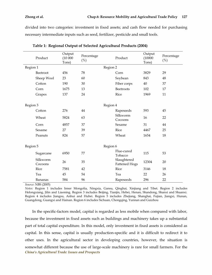
Zhong et al. Chap.6: Resource Mobility and Agricultural Trade Policy 127
China's Agricultural Trade: Issues and Prospects
divided into two categories: investment in fixed assets; and cash flow needed for purchasing
necessary intermediate inputs such as seed, fertilizer, pesticide and small tools.
Table 1: Regional Output of Selected Agricultural Products (2004)
Product Output (10 000 Tons)
Percentage (%)
Product Output (10000 Tons)
Percentage (%)
Region 1 Region 2
Beetroot 456 78 Corn 3829 29
Sheep Wool 23 60 Soybean 843 48
Cotton 190 30 Fiber corps 40 37
Corn 1675 13 Beetroots 102 17
Grapes 137 24 Rice 1969 11
Region 3 Region 4
Cotton 276 44 Rapeseeds 593 45
Wheat 5824 63 Silkworm Cocoons
16 22
Corn 4857 37 Sesame 31 44
Sesame 27 39 Rice 4467 25
Peanuts 824 57 Wheat 1654 18
Region 5 Region 6
Sugarcane 6950 77 Flue-cured Tobacco
115 53
Silkworm Cocoons
26 35 Slaughtered Fattened Hogs
12304 20
Rice 7581 42 Rice 3146 18
Tea 45 54 Tea 22 26
Bananas 584 96 Rapeseeds 296 22
Source: NBS (2005) Notes: Region 1 includes Inner Mongolia, Ningxia, Gansu, Qinghai, Xinjiang and Tibet. Region 2 includes Helongxiang, Jilin and Liaoning. Region 3 includes Beijing, Tianjin, Hebei, Henan, Shandong, Shanxi and Shaanxi. Region 4 includes Jiangsu, Anhui and Hubei. Region 5 includes Zhejiang, Shanghai, Fujian, Jiangxi, Hunan, Guangdong, Guangxi and Hainan. Region 6 includes Sichuan, Chongqing, Yunnan and Guizhou
In the specific-factors model, capital is regarded as less mobile when compared with labor,
because the investment in fixed assets such as buildings and machinery takes up a substantial
part of total capital expenditure. In this model, only investment in fixed assets is considered as
capital. In this sense, capital is usually production-specific and it is difficult to redirect it to
other uses. In the agricultural sector in developing countries, however, the situation is
somewhat different because the use of large-scale machinery is rare for small farmers. For the

Zhong et al. Chap.6: Resource Mobility and Agricultural Trade Policy 128
China's Agricultural Trade: Issues and Prospects
majority of agricultural producers in developing countries, small-scale agricultural tools are
usually used in production of various agricultural products. At the same time flexible capital
inputs, such as fertilizer and pesticides, which can be easily switched from production of one
crop to another, take up a larger share of the total capital inputs. Figure 1 shows the ratio of the
amount of tractor use in the United States to that of China, and the ratio of the amount of
fertilizer use in China to that of the United States. The figure shows clearly that China uses as
much as two times more fertilizer, and five to six times fewer tractors than the United States in
agricultural production.
Figure 1: Shares of Tractors and Fertilizer, China versus the USA
Source: FAO (2003)
Table 2 lists the proportion of different crop-specific production resources – fertilizer and
pesticides, machinery, and labor – in total inputs per unit of crop output in different countries
for the year 2000. It can be seen clearly that, for each unit of output of these agricultural
products, expenditure on flexible inputs such as fertilizer and pesticides are usually higher in
China than in other countries, especially developed countries, while investment in the relatively
immobile input machinery is much lower.
It could be inferred, therefore, that in Chinese agricultural production, the mobility of
capital is relatively high in comparison with that in developed countries, and there is not much
difficulty in transferring from the production of one product to another. However, the
constraint faced by farmers is the limited availability of capital. Consequently, the capital
0.0
1.0
2.0
3.0
4.0
5.0
6.0
7.0
1999 2000 2001 2002
Tractor: USA/China
1.65
1.70
1.75
1.80
1.85
1.90
1.95
2.00
2.05
2.10
Fertilizer: China/USA
Tractor Fertilizer

Zhong et al. Chap.6: Resource Mobility and Agricultural Trade Policy 129
China's Agricultural Trade: Issues and Prospects
constraints they might face in switching production are less an issue of mobility than that of
insufficiency of capital available.
Table 2: Proportion of Inputs in Agricultural Production in Different Countries (2000)
Crop Country Cost proportion of various inputs
Fertilizers & Pesticide % Machinery % Labor %
Wheat
China 22 16 35
USA 20 18 6
Canada 36 30 11
Corn China 23 10 46
USA 21 30 9
Soybean China 11 10 46
USA 14 27 8
Rapeseed China 19 6 54
Canada 41 28 9
Indica rice China 16 9 43
Thailand 29 24 37
Japonica rice China 20 16 36
USA 17 26 9
Source: Huang and Ma (2000)
Human Resources: Labor is another important production resource in the agricultural
sector in developing countries that deserves serious consideration when analyzing resource
reallocation. Mobility of labor is critically important in connection with open trade policy,
because compared with other economic or efficiency considerations, it is much more difficult to
find a satisfactory solution when labor is affected by foreign competition.
The mobility of agricultural labor should be analyzed from two different perspectives: as a
shift from one kind of production to another within the agricultural sector, and from
agricultural to non-agricultural production.
(i) Within the Agricultural Sector: consider first the case in which farmers engaged in one
kind of production switch to another kind of agricultural production. In China, as in many
other developing countries, obstacles to production changes exist to a varying extent. Natural
conditions, production concentration, and technology accessibility are the most obvious.
● Natural conditions and production concentration - as explained in the previous section,
the choice of production is to a large extent determined by the landscape and climate of a
region. Switching from one production type to another may or may not be feasible. Other than

Zhong et al. Chap.6: Resource Mobility and Agricultural Trade Policy 130
China's Agricultural Trade: Issues and Prospects
that, switching from one large-scale production type to another relatively new and unfamiliar
production type usually involves very high transitional costs and possibly a very slow
transition. Take Guangxi province in Region 5 as an example. Because of the favorable climate
and soil conditions, sugarcane production is prevalent and important in the region. More than
12 million farmers make a living from sugarcane production, and another 100,000 from sugar
processing. Tax from sugarcane is also the major source of local government revenue in a
significant number of counties in the region. It is, therefore, very difficult in this province to
shift sugar production to another kind of agricultural production within a short period, either
because of the large number of farmers or because of the local financial dependence. That aside,
shifting to new production might also be less profitable due to unfavorable natural conditions.
● Technological accessibility - this is another very important constraint for Chinese
farmers in switching from one production type to another. Deep-rooted traditions and rich
experience in one production activity make learning and dissemination of new technology
difficult, especially when farmers maintain low levels of education and rely heavily on skills
passed down from generation to generation. The agricultural technological extension services,
in contrast, are still weak in their capacity to provide sufficient support, with only 15 technical
personnel to every 10,000 farmers in the country compared with that of 100 in Japan and 200 in
the Netherlands. The insufficiency of agricultural extension services makes it risky for farmers
to switch to unfamiliar production that requires the adoption of new technology.
In addition to the lack of technological support, farmers also face the risk of fake new
varieties and inputs such as pesticides, fertilizers etc., which makes farmers even more afraid of
switching to unfamiliar production activities. In Shanxi province, 177 households in Pingyao
County bought a new variety of watermelon seeds in the hope of making a good profit for the
year. However, after months of hard work on 500 mu of their land, what was waiting for them
was no harvest at all. It turned out that the seeds were not qualified varieties but had been
illegally sold on the black market. The illegal selling was not punished, and the farmers were
not fully compensated and had to bear most of the loss themselves. The lack of a well-
established and functioning legal system to resolve disputes adds another obstacle to farmers‘
ability to switch to new types of production.
(ii) From Agricultural to Non-agricultural Sector: the mobility of labor in the agricultural
sector in China is both constrained by its quantity and low quality, as well as by institutional

Zhong et al. Chap.6: Resource Mobility and Agricultural Trade Policy 131
China's Agricultural Trade: Issues and Prospects
barriers. The immobility becomes more apparent when migration from rural to
urban/industrial sectors is considered.
In terms of quantity, there are various estimates of the ―floating population‖ (rural laborers
seeking city jobs) ranging from 90 to 140 million, depending on the source. But the actual
amount of surplus labor is much greater than these estimates, because underemployment in the
agricultural sector is prevalent. In contrast, non-farm job opportunities are extremely limited
compared with the amount of rural surplus labor, and the situation is worsening due to the
continuous laying-off of workers in cities in recent years. The official unemployment rate in
urban areas reached 7–8% in 2002, which is believed to be an underestimate by many
researchers and does not take unemployed rural immigrants into consideration, making it more
difficult for rural laborers to move to urban areas. Moreover, both the reform of state-owned
enterprise and government policy for attracting foreign investment are capital and technology-
intensive. The capital and technology-intensive development strategy adopted in the industrial
sectors has dampened labor absorption capability during decades of economic growth. At
present, the employment elasticity of GDP growth is 0.1 in China, compared with an average of
0.3–0.4 in other developing countries.
In terms of quality, the education level of rural laborers is generally lower compared with
their urban counterparts. Survey data show that about 20–30% of migrants from rural to urban
areas have received only primary school education or lower and only 10–20% received
education at the senior high school level or above. In contrast, most employers in cities have
explicit requirements for education, usually above junior high school, and many require a
certain level of employment experience and/or training. The incompatibility of supply and
demand in the labor market makes the transition of labor movement from rural to urban areas
even harder.
Other barriers also affecting the mobility of rural laborers in China are as follows:
● Household registration system - rural migrants have long been constrained by the
household registration system, which prevents them from staying in cities for long periods of
time and/or looking for jobs. Even after the relaxation and deregulation of many of the
restrictions on migrants, certificate requirements and discriminatory treatment in practice still
make it very difficult for immigrants to stay and work in cities for long periods of time.

Zhong et al. Chap.6: Resource Mobility and Agricultural Trade Policy 132
China's Agricultural Trade: Issues and Prospects
● Lack of social safety nets - farmers moving into cities are in desperate need of rights that
protect basic working and living conditions, as well as the right to basic education for the next
generation. At present, migrants employed in cities are paid the lowest and work under the
poorest conditions, and their children of school age cannot be enrolled in a local school without
the payment of a large sum of money.
● Lack of financial capability and necessary information - some surveys show that most
rural migrants are farmers with a household income of above average for their rural locality.
Lack of basic necessary financial support prevents a large number of extremely poor farmers
from migrating in search of better opportunities. Migrants must usually be self-reliant or use
their limited connections with friends in the target urban area to find urban jobs. Job
information services for migrant farmers are still far from adequate. All these obstacles hamper
the ability of rural laborers to move to the urban sectors.
Institutional Arrangements: There are many other institutional arrangements in the
transitional period that greatly restrict the mobility of labor, especially that from rural to urban
areas. Social security programs are examples of such institutional arrangements. Pension, health
care, and subsidized housing, were all established under the planned economy and attached to
a specific region and/or industry, or even to individual enterprises or institutions. Although
many reforms have been implemented in social security programs, the Chinese labor force in
the urban/industry sectors must still go to their individual employer to obtain such benefits.
The design of such programs was probably for convenience and subject to financial constraints
at the time, but it has worked against mobility of the labor force, preventing full integration of
the labor market.
Because China has not yet established a nationwide social security system, pension and
health-care programs are usually run only in the urban/industrial sectors, and are region-
and/or industry-, or even enterprise-specific. It is difficult for ordinary factory workers to
transfer their accounts or benefits when moving to other places. Because those already-
employed workers are not able to leave their existing positions, no vacancies are available to
others, and the situation is even harder for new immigrants from the rural areas. The existing
social security programs are designed to protect current employees, subject to financial resource
constraints in each region, industry, or enterprise. Naturally, it excludes outsiders, but rural

Zhong et al. Chap.6: Resource Mobility and Agricultural Trade Policy 133
China's Agricultural Trade: Issues and Prospects
immigrants are affected much more heavily because most such programs are region- and/or
industry-specific, and thus benefit local residents.
The expected benefits from pension and health care, as well as some other social security
programs, are also based on the ownership status of the respective employer. Benefits provided
to civil servants are different to those enjoyed by employees of public institutions such as
universities and research institutes, or to those enjoyed by employees of state-owned enterprise,
or by employees of private enterprise. Therefore, the existing social security programs that have
restricted labor mobility to a significant extent partly contribute to the low level of integration in
the labor market.
Another, and probably most severe, obstacle to labor mobility is the cost of housing. The
nature of subsidies in urban housing makes it similar to a social security program. For a long
time before the mid-1990s, the Chinese government provided virtually free housing to state
employees through their employers, and to other urban residents through state housing
agencies. Of course housing conditions varied greatly across regions, industries, and
institutions. But the costs for existing residents were kept very low even when the housing
market emerged in the 1990s. When the privatization of residential housing in the mid-1990s
commenced, most apartments were sold to existing residents at a nominal price, which was
usually equivalent to 5–10% or less of their market value. Because housing costs have never
been reflected in wage reforms, all those who entered the job market now face major problems
if they have no housing or cannot share housing, say, with their parents who were beneficiaries
of the housing reform.
The current market price for a two-bedroom apartment in a big city is approximately equal
to 20 times the annual salary for a factory worker, or even higher, depending on location and
other conditions. Urban youth with higher education may earn a higher income and receive
help from their parents who purchased housing after the reform, but rural immigrants with a
lower education cannot find decent housing for themselves in cities. Without permanent
housing, immigrants cannot claim local residential status nor can they enjoy some of the basic
social security programs, and their children are denied access to low-cost public primary school
education.
The above examples demonstrate that the Chinese labor force is divided into a variety of
categories: by region, by industry, by ownership etc. However, the deepest division is between
Zhong et al. Chap.6: Resource Mobility and Agricultural Trade Policy 134
China's Agricultural Trade: Issues and Prospects
urban and rural residents, because the latter enjoy very few social security benefits. Naturally,
such a division in social program coverage has been an important barrier to labor mobility, and
has worked against immigrants from rural to urban areas. The continuous reforms in social
security programs and related institutions will gradually narrow the gap between categories,
and finally lead to an integrated labor market. However, this is likely to be a long process, and
the immobility of rural laborers and their resultant low incomes will continue to be an
important subject of public policy, including trade policy, during the transitional period.
Agricultural Resource Mobility and Trade Policy in China
As in many other developing countries, China‘s agricultural trade policy has been reworked to
accommodate domestic issues and to serve the national development goal of industrialization.
China was a net grain exporter in the 1950s, although grain output was not high enough to meet
domestic demand. But due to the compulsory food procurement and rationing system aimed at
mobilizing all available agricultural resources to speed up industrialization, grain was exported
to earn foreign exchange, which in turn was used to import necessary industrial products. The
famine of the late-1950s to the early-1960s turned China into a net grain importer with the
quantity controlled at the minimum level by the state. Because agricultural production was
controlled by the state and aimed at grain self-sufficiency, such trade was not a mechanism to
improve resource allocation efficiency, and had not taken into account resource mobility at all.
From the early-1980s onward, net grain imports were increased to more than 15 million
metric tons, over 4% of total domestic consumption, although domestic production was also
experiencing significant growth in China following the 1979 reform. The objective of the
increased imports, under the State plan, was twofold: (1) to improve production incentives in
the urban/industrial sector with increases in the food supply, and (2) to release production
resources for more sugar and cotton production, as sugar and cotton are necessary materials for
domestic processing factories, and are also more profitable to produce domestically than to
import. In this case, a share of the imported grain was allocated to producers of major cash
crops such as cotton and sugar, reducing the burden of grain production for their own
consumption. Although the substitution of sugar and cotton for grain production was aimed at
saving foreign exchange and to promote industrialization, it improved resource allocation
efficiency in the agricultural sector as a whole, and it also raised the income of farmers who
were permitted to shift all or part of their grain production to cash crops. However, this kind of

Zhong et al. Chap.6: Resource Mobility and Agricultural Trade Policy 135
China's Agricultural Trade: Issues and Prospects
resource reallocation was not fully realized, because major cash crop producers were still
required to produce grain for their own consumption, and other farmers were still under
compulsory mandates for grain production. Self-sufficiency remained a top priority for the
country and was implemented via the State under the compulsory procurement program. Thus
the production resources and mobility of farmers were still largely suppressed.
Reforms in the agricultural market that took place in the 1980s and 1990s and which
gradually increased farmers‘ decision-making power and allowed for improvement in their
resource allocation, was an important approach to increasing both agricultural supply and farm
income. In the late-1990s, the low income of farmers, which was due to immobility of their
production resources and inability to switch to other forms of production, was dealt with
directly by government policy. For the first time, the State established protective prices that
were above the market level for some selected grain crops, for example corn produced in
Northeast China and indica rice in Central China. Farmers in the two regions had few
alternatives other than to engage in corn or rice production, where immobility of production
resources resulted from long-term concentration of corn and rice production, respectively.
Protective prices and associated government subsidies were introduced in recognition of the
immobility of resources in these regions, and as compensation for farmers who suffered low
prices as a result of domestic and international competition.
The goal of agricultural production and trade policy in China has changed remarkably,
shifting from ensuring production to improving farm incomes. The subsidy to corn producers
in Northeast China, while providing trade protection from international competition, is in fact
aimed more at improving farmer‘s welfare than at increasing the domestic output. It implies
that, if corn producers improve their production resource mobility and can be shifted out of
corn production to make a profit, the policy would be terminated even if output would be
lower. As such, protective trade policy could in fact be reconsidered in comparison to other
policy alternatives, such as policy measures to improve farmers‘ resource mobility, which might
come at lower cost.
Conclusion and Policy Implications
This chapter examines the mobility of different production resources in Chinese agriculture:
natural resources, capital inputs, human resources and institutional arrangements. The analysis
shows that most production resources in Chinese agriculture are low in mobility. Natural

Zhong et al. Chap.6: Resource Mobility and Agricultural Trade Policy 136
China's Agricultural Trade: Issues and Prospects
variation in climate, soil and water leads to concentration of production in different regions; a
low level of education and lack of accessibility to technology make the conversion of production
within the agricultural sector difficult; a large amount of surplus rural labor and the slow
growth of urban job opportunities result in limited inter-sector migration of rural human
resources; and existing institutional arrangements further add to the difficulties present in
human resource movement.
The low resource mobility in Chinese agricultural production has significant policy
implications. On the one hand, preference for policies that protect certain crops in certain areas,
and where production is concentrated and producers have little alternative for other sources of
income, is legitimate and necessary, at least in the short run. When compared with farmers in
developed countries, agricultural producers in China are not only a much larger group, but are
also more vulnerable because of their much lower and volatile income. This also has significant
implications for disadvantaged groups, such as those in poverty and women. As studies and
surveys show, rural labor migrants consist mainly of males who come from families of middle-
income and above. Women and poor farmers have less mobility, and are more vulnerable to
income shock. Therefore, trade protection for a transitional period of time is necessary to avoid
social instability and allow time for readjustment.
On the other hand, policy instruments should be explored and implemented to improve
resource mobility in the Chinese agricultural sector. Investment in rural education and skill
training, in transportation and communication infrastructures, could be expanded. In particular,
policy alternatives to improve resource mobility should be explored, as well as alleviation of
poverty in the transitional period. Further market-oriented reform to eliminate all institutional
barriers and the establishment of social security nets for rural people would also be effective
measures to improve resource mobility in the agricultural sector. The ongoing ―Development of
New Rural Society in China‖, which is aimed at providing better production, living and
development conditions for farmers, is a good start.
From the perspective of policymaking, the costs of protecting a specific sector should be
compared with the potential costs of improving mobility of relevant resources, especially that of
laborers. The comparison might be useful in assessing whether protection of production or
improvement of resource mobility is more preferred in the short run. It is anticipated that, in the
long term, government policy to improve resource mobility in the agricultural sector and to

Zhong et al. Chap.6: Resource Mobility and Agricultural Trade Policy 137
China's Agricultural Trade: Issues and Prospects
implement a gradual pro-open policy will prove to be more beneficial for both the rural
population and the economy as a whole. It is also of significant importance to enhancing farm
income, as well as in reducing trade disputes.
References
Blanchard, O. and L. Katz. ―Regional Evolution.‖ Brooking Papers on Economic Activity ?(1992): 1–
75. Brecher, R. and E. Choudhri. ―Pareto Gains from Trade, Reconsidered: Compensating for Jobs
Lost.‖ Journal of International Economics 36(1994): 223–238. Burgon, B. ―Globalization and Welfare Compensation: Disentangling the Ties that Bind
International Organizations.‖ International Organization 55(2001): 509–551. Cai, F. ―Analysis of Institutional Barriers to Migration of Rural Surplus Labor.‖ Economics
Information 1(2005): 35–39. Cassing, J. and J. Ochs. ―International Trade, Factor Market Distortions, and the Optimal
Dynamic Subsidy: Comment.‖ American Economic Review 681978): 950–955. FAO. FAOSTAT. Rome: FAO (2003). (Available from http://faostat.fao.org) Huang, J. and H. Ma. ―Production Costs of Major Farm Commodities in China: International
Comparison and Difference.‖ Chinese Rural Economy 5 (2000): 17–21. Huang, J., Z. Xu, N. Li and S. Rozelle. ―Trade Liberalization and China‘s Agriculture, Poverty
and Equality.‖ Issues in Agricultural Economy 7(2005): 9–14. National Bureau of Statistics of China. China Statistical Yearbook. Beijing: China Statistics Press,
2005. National Bureau of Statistics of China. Chinese Agricultural Statistical Yearbook. Beijing: China
Statistics Press, various years. Zhao, Y. ―Rural Labor Migration and the Role of Education.‖ Economic Research 2 (1997): 37–42. Zhong, F. ―Attack or Defense: Strategic Choice of the Focus of Agricultural Support Policy.‖
Issues in Agricultural Economy 1 (2003): 55–59.

Anderson et al. Chap.7: Long Run Implications of WTO Accession 138
China's Agricultural Trade: Issues and Prospects
Chapter 7:
Long Run Implications of WTO Accession for Agriculture in China
KYM ANDERSON WILL MARTIN
ERNESTO VALENZUELA
The World Bank
Anderson et al. Chap.7: Long Run Implications of WTO Accession 139
China's Agricultural Trade: Issues and Prospects
Long Run Implications of WTO Accession for Agriculture in China
Chapter 7:
Introduction
In recent years, a standard approach to evaluating the welfare effects of trade agreements has
been widely used. This approach begins by assessing the applied rate of protection in place
before the agreement. It then examines the commitments made under the agreement—
commitments such as tariff bindings made under World Trade Organization (WTO)
agreements, or commitments made under preferential arrangements. Where these
commitments are below the initially applied rates—the most-favored-nation (MFN) tariffs in
the case of WTO commitments, or the applied rates under regional arrangements—it is
assumed the applied rates will be reduced to respect the commitments. After comparing the
bound and applied tariffs at the finest possible level of product disaggregation, the tariffs are
aggregated to the level needed for quantitative analysis.
This approach seems a substantial improvement over the simpler approach widely used in
earlier evaluations of trade reforms (see, for example, Brandão and Martin, 1993) and still used
in studies such as Polaski (2006) where the stylized nature of the tariff reduction is captured in a
measure such as a 36 percent cut in applied tariff rates. While policy agreements are sometimes
described in simplified terms such as this, the devil is frequently in the details, and the impact
on applied tariffs is likely to be quite different from the description when these details are taken
into account (see Hathaway and Ingco, 1995). Now that data on applied tariffs and bindings are
available on an ad valorem basis for standardized commodities at the six-digit level of the
Harmonized System, it can take into account a great deal of information that was ignored in
earlier studies. This broad approach was used in (Anderson and Martin, 2006), and is now
incorporated in the tariff analysis feature of software programs such as WITS
(www.wits.worldbank.org).
A key challenge for this type of analysis lies in the counterfactual, i.e., what would applied
tariffs have been in the absence of the agreement? Here, there are two particularly interesting
cases for analysis of agricultural trade reforms. The first is the short-run impact of the tariff

Anderson et al. Chap.7: Long Run Implications of WTO Accession 140
China's Agricultural Trade: Issues and Prospects
reductions on variables such as agricultural output, trade levels and farm incomes. The second
is the potential long term implications of these commitments.
The standard approach to specifying the counterfactual level of protection is appropriate
for short-run analysis, although there is frequently some ambiguity. Ianchovichina and Martin
(2004) for instance, assumed that most of the tariff reductions associated with China‘s accession
to the WTO, were actually undertaken before China joined the WTO, as China sought to
establish her bona fides for the market-oriented WTO system. A similar ambiguity arises in
analyses of the Doha negotiations with Europe‘s pre-announced liberalization of agricultural
trade policies. Should such policies be treated as part of the counterfactual, even though they
are not locked in through WTO commitments and hence are potentially reversible?
For analyses of longer-run impacts, the specification of the counterfactual is even more
challenging. We know that the appropriate counterfactual depends on secular changes in both,
the level of protection of the type analyzed by Anderson and Hayami (1986) and in the
variability of that protection over time (Francois and Martin, 2004). It also depends on the
important questions raised in recent research by Melitz (2003) and Kehoe and Ruhl (2003): to
what extent would a more liberal regime result in growth of exports and imports at the
extensive margin—that is through the emergence of new varieties and new products - as
distinct from through increases in the quantities of goods initially traded?
In the case of China‘s accession to the WTO, it is particularly important to recognize that,
prior to accession to the WTO, most of the important agricultural trade barriers in China were
implemented through measures such as state trading, import and export quotas and licenses
(Ianchovichina and Martin, 2004), rather than through trade taxes. Tariff rates for imports of
many commodities were high, while the protection actually delivered appears to have been
very low or negative for many of these commodities (see Huang, Liu, Martin and Rozelle, 2007).
Studies such as that by Schmidhuber (2001), which use initial applied tariff rates, tend to
overstate the short-run impact of liberalization by overstating the amount of protection actually
delivered to domestic producers. In this chapter, we draw on new estimates of protection
actually delivered to producers and consumers in 2004, as provided by Huang, Liu, Martin and
Rozelle (2007).
In the long run, however, there is a risk that our standard approach to welfare evaluation
may understate the benefits of reform. In the absence of commitments such as those China

Anderson et al. Chap.7: Long Run Implications of WTO Accession 141
China's Agricultural Trade: Issues and Prospects
made under the WTO, it seems reasonable from the experience of other East Asian economies to
assume that farm protection might have risen substantially for political-economic reasons. It
also seems likely that this protection would have varied more from year to year, potentially
increasing the cost of protection by a substantial margin (Francois and Martin, 2004). Further,
the more liberal approach embodied under the WTO is likely to result in an expansion in the
range of products traded. Our empirical focus in this chapter is on the first of these weaknesses
in the standard approach, although we address also the other two in a less formal manner.
To do this, we take advantage of new assessments of levels and trends in agricultural
protection in China and other East Asian economies emerging from a new World Bank project
on global agricultural distortions (Anderson, 2008). The estimates for the higher-income East
Asian countries update and expand on earlier estimates of agricultural protection in the region
(Anderson and Hayami, 1986), and estimates for the other 80 countries included in the analysis
allow us to put it in a broader context. New estimates for that project for China (Huang et al.,
2007) allow us to examine the stance of China‘s agricultural policies back to the early-1980s,
when China‘s current generation of farmers first became thoroughly responsive to market
prices.
In this chapter, we consider first the relationship between national agricultural trade
policies and multilateral trade rules. Then, we consider the evolution of agricultural trade
distortions in China during the reform era, and place this evolution in the context of the
experience of other East Asian economies whose rapid economic growth first occurred when
WTO rules on agricultural trade were weak or ineffective. With this as background, we examine
what might be the driving forces behind these changes in protection. Then we consider the
nature of the commitments on agricultural trade policies associated with China‘s accession to
the WTO. Finally, we re-examine empirically the long run impact of China‘s accession to the
WTO, using the GTAP model of the global economy. In doing so, we consider the implications
for China of alternative policy options for dealing with the very real problems of transition
associated with China‘s rapid industrialization and the inevitable relative decline of agriculture
that will continue to accompany its rapid economic growth.
Agricultural Trade Policy and the GATT
The key principles of the multilateral trading system—non-discrimination, transparency, the
use of tariffs rather than non-tariff measures for protection, and disciplines on the level of

Anderson et al. Chap.7: Long Run Implications of WTO Accession 142
China's Agricultural Trade: Issues and Prospects
protection —are just as relevant to agriculture as to other merchandise trade. Unfortunately,
however, these principles were severely compromised during the evolution of the multilateral
trading system. For farm products nontariff barriers were allowed, tariffs were essentially
unrestrained, and even export subsidies were permitted.
A consequence of these developments was a progressive deterioration in international
markets for agricultural products, a situation characterized by Johnson (1991) as one of
―Agriculture in Disarray‖. High and rising protection, and the use of domestic and export
subsidies, reduced the trend level of international agricultural prices and increased their
volatility (Tyers and Anderson, 1992). Much of the protection and market insulation provided
by the major industrial countries was wasted—seeking merely to offset the adverse impacts of
distortions in other markets on world prices. Further, the pattern of distortions was regressive
from the point of view of global farm income distribution. Farmers in rich countries—and
especially larger farmers—were heavily protected while farmers in poor countries were taxed
(Krueger, Schiff and Valdes, 1988). It was clear to any dispassionate observer that reform was
needed in both rich and poor countries. Given the strong political-economic support for
agricultural protection in the industrial countries, it seemed that the only feasible approach to
reducing these barriers would be through international negotiations. A negotiated outcome
provided at least the hope of finding a better alternative to continuation of the sporadic trade
wars that had come to characterize agricultural trade in the absence of multilateral disciplines.
This recognition contributed to the decision of GATT contracting parties to include
agriculture in the Uruguay Round negotiations. Despite the well-known difficulties in reaching
agreements for this sector, one was reached by 1994 (GATT, 1994) that provided a framework
for managing international trade in agriculture, including replacement of non-tariff barriers by
tariff measures and the introduction of disciplines on export subsidies and domestic support.
While it had limited success in reducing protection from the levels that it had attained in richer
countries (Hathaway and Ingco, 1996), it appears to have contributed to restraining the
increases in protection in the industrial countries that had previously seemed to be inexorable
(OECD, 2006).
Since the Uruguay Round, the procedures for accession to the multilateral trading system
appear to have become considerably more rigorous for developing countries (Martin, 2007).
This was particularly the case for China, whose accession to WTO was a major event both for

Anderson et al. Chap.7: Long Run Implications of WTO Accession 143
China's Agricultural Trade: Issues and Prospects
China and for the WTO membership, and who undertook reforms that generated substantial
benefits both for China and her major trading partners (Bhattasali, Li and Martin, 2004). Some
have noted that these reforms involved major changes in agricultural tariffs, but this ignores the
fact that most of the protection (and taxation) of China‘s agriculture prior to accession arose
from non-tariff measures such as state trading. Detailed analysis by Huang, Rozelle and Min
(2004) takes this into account and shows that the reductions in applied protection to agriculture
in China were much smaller than would be implied by the changes in tariffs required by
accession.
The Evolution of China’s Agricultural Distortions
While it is well known that trade and pricing policies in poor countries have tended to tax
farmers, the evidence on this issue has been much less clear cut for China than for other
countries. Some studies examining this issue with price comparisons based on official exchange
rates have tended to suggest that farmers in China were protected during the early reform
years. However, during the socialist period, a key objective was to accelerate the rate of
industrial development, and policy came to finance part of that through direct and indirect
transfers from agriculture (Mao Zedong, cited in Lardy, 1983, p.17).
During the planning era, the prices of agricultural products also appear to have been
depressed to allow food to be sold at low prices to urban consumers—a pattern consistent with
that observed in other low income countries (Pinstrup-Andersen, 1988). Guo Shutian estimates
the ‗scissors difference‘—the extent to which the agricultural sector was taxed by the prices of
agricultural goods being set below their market values and the prices of industrial goods being
set above what would have been their free-market level. That policy involved total taxation of
agriculture of an estimated 26 percent in 1957 and 27 percent in 1978, primarily from direct
taxation of the prices of agricultural goods (reported in Yao, 1994, p.138).
Once adjustments are made for the dual exchange rate regime that prevailed from the
early-1980s until unification of the exchange rate in 1994, however, it is possible for a
comparison of China‘ domestic prices with international prices to be used to make inferences
about the implications of China‘s trade and pricing policies for agricultural incentives. Such
comparisons are important because agricultural trade was managed using a wide range of non-
transparent policies, including state trading, licensing and quotas as well as tariffs. During this

Anderson et al. Chap.7: Long Run Implications of WTO Accession 144
China's Agricultural Trade: Issues and Prospects
period, the household responsibility system was in effect, so price incentives affected not only
the real incomes of producers and consumers but also actual production decisions.
Huang et al. (2007) provide estimates of protection and taxation for 11 commodities: rice,
wheat, maize, soybeans, cotton, pork, milk, poultry, fruit (using apples as a representative
product), vegetables (using tomatoes as a representative product) and sugar (both sugar-beet
and sugarcane) between 1981 and 2005. Over their study period, these commodities accounted
for between 75% (in the late-1980s) and 60% (during the early-2000s) of the total value of
agricultural output in China. A summary of their key results is given in Table 1.
Table 1: Nominal Rates of Assistance to Agricultural Industries, China, 1981-2005
Crop 1981-84 1985-89 1990-94 1995-99 2000-05
Exportables* -51.3 -46.4 -21.0 -0.7 -0.2
Rice -54.2 -34.0 -30.4 -6.6 -7.2
Fruits -24.6 -9.4 -18.0 0.0 0.0
Vegetables -37.8 -57.5 -44.6 0.0 0.0
Poultry 27.1 -27.1 -27.6 0.0 0.0
Pork -75.5 -48.8 -34.4 0.0 0.0
Import-competing* -22.0 12.1 -5.3 19.5 7.5
Wheat 5.0 22.3 11.3 30.2 4.0
Soybeans 2.8 1.3 4.7 29.5 16.3
Sugar 43.7 44.7 11.7 26.6 29.4
Milk 153.9 58.3 -4.3 18.3 24.8
Mixed trade status*
Maize -32.8 -16.1 -25.1 5.3 12.6
Cotton -30.2 -34.6 -26.2 -3.6 0.7
Weighted average of above products* -47.4 -41.7 -19.9 -0.1 0.6
Standard deviationa 79.5 53.1 24.6 19.5 15.6
Coverage as % of value of total agricultural production (at undistorted prices) 84.6 89.3 88.4 82.2 69.1
Source: Huang et al. (2007) * Nominal Rates of Assistance to farmers plus product-specific input subsidies weighted using the value of output at undistorted prices. Mixed trade status products included in exportable or import-competing groups depending upon their trade status in the particular year a The standard deviation shown is the simple 5-year average of the annual standard deviation around the weighted mean
Anderson et al. Chap.7: Long Run Implications of WTO Accession 145
China's Agricultural Trade: Issues and Prospects
A striking feature of Table 1 is the extent to which producers were directly taxed by
agricultural and trade policies in the early reform era. This was particularly the case for staple
foods such as rice and maize. Taxation of rice reduced returns to farmers by over 50% relative to
world price levels. Cotton prices were also strongly depressed, partly because of a desire to
have low cost inputs for the processing sector. Returns to other labor-intensive agricultural
products such as vegetables and pork were also depressed, partly as a consequence of
restrictions on exports. Returns to import-competing agricultural products were much less
seriously depressed, and some of these products, such as sugar and milk, had quite high levels
of positive protection. For these products, the goal of self-sufficiency, or at least concerns about
vulnerability if grain imports reached double-digit shares of consumption, appear to have
resulted in much lower levels of taxation. Protection to agricultural exportables and to maize
and cotton remained strongly negative in the late-1980s, while protection to imported
commodities became slightly positive.
In the first half of the 1990s, there were very important changes, including the abolition of
the system of compulsory procurement of grains. The weighted average rate of taxation fell by
half in this period to just below 20%. However, key commodities such as rice, maize and cotton
still had negative rates of assistance. In the late-1990s, the taxation of rice diminished greatly,
and taxation of a range of other exportable goods disappeared as export restrictions on these
goods were removed.1 Taxation of import-oriented agriculture disappeared completely, to be
replaced by significant agricultural protection. In part, this reflected the phase-out of the
obligation for farmers to deliver a substantial amount of their output at below-market prices
under the production quota system. Incentives for maize protection became positive in this
period, with export subsidies applying in at least some years (Huang, Rozelle and Min, 2004).
Between 2000 and 2005, direct protection to agriculture became, on average, essentially zero,
with protection to both importable and exportable goods reaching low levels.
1 Prices for these goods still tended to be below world prices, but this was more a consequence of foreign barriers, than of barriers imposed by China, which were the focus of this study.

Anderson et al. Chap.7: Long Run Implications of WTO Accession 146
China's Agricultural Trade: Issues and Prospects
Figure 1: Nominal Rates of Assistance to Rice, Wheat and Maize, China, 1981-2005 (%) Panel A. Rice
Panel B. Wheat
Panel C. Protection to Maize, Conditional on Trade Status, %
Source: Huang et al. (2007)
RICE
-70
-60
-50
-40
-30
-20
-10
0
10
80 85 90 95 00 05
%
NRAf
NRA
WHEAT
-40
-20
0
20
40
60
80
100
80 85 90 95 00 05
% NRAf
NRA
MAIZE
-60
-50
-40
-30
-20
-10
0
10
20
30
40
80 85 90 95 00 05
% NRAf
NRA

Anderson et al. Chap.7: Long Run Implications of WTO Accession 147
China's Agricultural Trade: Issues and Prospects
Annual movements in the protection rates applied to key commodities are given in Figure
1, taken from Huang et al. (2007). The Nominal Rates of Assistance for farmers (NRAf) for rice
in Panel A shows the extent of taxation to farm returns for rice. When the obligation to make
quota deliveries at below-market prices applied, the depressed procurement prices accounted
for a substantial amount of the reduction in farm returns. While these prices were to some
degree decoupled from the marginal incentives to producers (Sicular, 1988), they were not fully
decoupled in that they did influence the incentives for farm households to stay in agriculture.
The graphs in Figure 1 show the sharpness of the change in policies in the mid-1990s, when
the procurement system was abolished and prices were allowed to rise much closer to world
levels. While protection to rice was, on average, still negative, the rates of protection were very
low. For wheat, market prices had always been above world prices, but farm prices were, until
the abolition of the procurement system, below world prices. Following its abolition, protection
rates at the farm level were, on average, slightly positive. For maize, protection rates at the farm
level became positive after 1994, despite the fact that maize is generally an exportable. This was
partly due to the presence of export subsidies on maize and on cotton, which were ruled out by
China‘s WTO commitments.
Figure 2: Nominal Rates of Assistance to Agricultural and Non-Agricultural Tradeables, and
Relative Rates of Assistancea - China, 1981-2005 (%)
Source: Huang et al. (2007)
a The relative rate of assistance is calculated as RRA = 100[(100+NRAag)/(100+NRAnonag) - 1], where NRAag and NRAnonag are the nominal rates of assistance to agricultural and non-agricultural tradeables, respectively
-80
-60
-40
-20
0
20
40
60
82 85 88 91 94 97 00 03
NRA ag
NRA nonag
RRA
Anderson et al. Chap.7: Long Run Implications of WTO Accession 148
China's Agricultural Trade: Issues and Prospects
Another important influence on the incentive environment for China‘s agriculture is
protection to the non-agricultural sector. Protection to non-agricultural sectors imposes an
implicit tax on the agricultural sector by competing resources away from agriculture. Indeed
Krueger, Schiff and Valdés (1988) found this indirect taxation of agriculture, to be a greater
burden on developing-country agriculture than direct taxation of the type observed above for
rice in China. As part of the process of WTO accession, protection rates to both agriculture and
manufacturing were reduced substantially, and these reductions were locked-in through tariff
bindings. The relative rate of assistance (RRA) depicted in Figure 2 provides a simple summary
measure combining the effects of direct and indirect incentives. From the figure, it is clear that
the combined effect of reductions in direct taxation and indirect taxation through protection to
other sectors outweighed the effect of reductions in protection to protected agricultural sectors
in the late-1990s and early-2000s, and improved the overall incentives for agricultural
production in China.
The trends in China‘s agricultural protection have important implications for the estimating
the impact of WTO accession. Even though formal tariff rates on many agricultural
commodities were high, the rates of applied protection were generally low, as we have seen.
Further, WTO commitments generally affected only imported commodities and those subject to
prohibited export subsidies.
China’s WTO Accession Commitments
China‘s WTO accession commitments were extraordinarily comprehensive, covering tariffs,
non-tariff barriers, services trade reform and a wide range of regulatory aspects of trade,
including introduction of an automatic right to trade in goods, as distinct from the positive-list
approach that had previously prevailed. An important feature of the agreement was an
emphasis on non-discrimination and transparency. As noted by Kehoe and Ruhl (2003), the
effect of such comprehensive reforms, which create many market opportunities, and create
greater confidence in the stability of the trade regime, may well have impacts that go well
beyond the effects of the changes in trade barriers. However, estimating the impact of these
barriers provides a useful lower-bound initial estimate.
While China‘s trade regime for non-agricultural commodities included a plethora of non-
tariff measures, their protective impact appears to have been relatively small by the time of
China‘s accession, at perhaps around 5 percent of the value of trade (Ianchovichina and Martin,

Anderson et al. Chap.7: Long Run Implications of WTO Accession 149
China's Agricultural Trade: Issues and Prospects
2004). Given the uncertainty about the distribution of this protection across commodities, we
focus on the impacts of tariff protection in order to obtain a lower-bound estimate of the impact
of accession. The estimates of tariff protection in 1995 used in this analysis are presented in
Table 2.
Table 2: Estimates of Tariff Protection in China, 1995 and 2001 (%)
1995 2001 Post-accessionb
Agriculture
Rice –5.0 –3.3 –3.3
Wheat 25.0 12.0 12.0
Feed-grains 20.0 32.0 32.0
Vegetables and fruits –10.0 –4.0 –4.0
Oilseeds 30.0 20.0 3.0
Sugar 44.0 40.0 20.0
Plant-based fibers 20.0 17.0 20.0
Livestock and meat –20.0 –15.0 –15.0
Dairy 30.0 30.0 11.0
Processed food 20.1 26.2 9.9
Beverages and tobacco 137.2 43.2 15.6
Total 4.8 7.6 3.6
Manufacturing
Extractive industries 3.4 1.0 0.6
Textiles 56.0 21.6 8.9
Apparel 76.1 23.7 14.9
Light manufactures 32.3 12.3 8.4
Petrochemicals 20.2 12.8 7.1
Metals 17.4 8.9 5.7
Automobiles 123.1 28.9 13.8
Electronics 24.4 10.3 2.3
Other manufactures 22.0 12.9 6.6
Total 25.3 13.5 6.9
Total merchandise tradea 24.3 13.3 6.8
Services
Trade and transport 1.9 1.9 0.9
Construction 13.7 13.7 6.8
Communications 9.2 9.2 4.6
Commercial services 29.4 29.4 14.7
Other services 24.5 24.5 12.7
Total 10.3 10.3 5.2
Source: Ianchovichina and Martin (2004) a Estimates are based on trade weights for the respective years b Applied rates at the end of the implementation period were estimated as the lesser of the bindings and 2001 applied rates
Examination of the estimates of weighted average protection rates for 1995, 2001 and after
accession presented in Table 2 suggests that substantial merchandise trade liberalization

Anderson et al. Chap.7: Long Run Implications of WTO Accession 150
China's Agricultural Trade: Issues and Prospects
occurred in China over the period 1995–2001. Weighted average protection dropped
substantially for wheat, beverages and tobacco, textiles, apparel, light manufactures,
petrochemicals, metals, automobiles, and electronics. Analysis by Huang et al. (2007) suggests
that some agricultural commodities such as vegetables and fruits, livestock and meat, and rice
faced negative protection prior to accession, generally as a result of restrictions on exports.
Protection on these commodities rose (or negative protection fell) over the period 1995–2001.
Accession did not lead to a significant fall in protection on most agricultural commodities after
2001. Indeed import protection remained unchanged for most commodities except oilseeds,
sugar, and dairy products.
Protection continued to fall for all other merchandise commodities, with especially big cuts
for processed food, beverages and tobacco, automobiles, electronics, and other manufactures. A
key element of China‘s accession agreement was the abolition of agricultural export subsidies.
This required some significant changes. Huang, Rozelle, and Min (2004) estimate that there was
a 32 percent export subsidy on feed-grains and a 10 percent export subsidy on plant-based
fibers (particularly cotton) in 2001.
China’s Agricultural Protection in an International Context
As we have seen, there have been substantial changes in China‘s agricultural distortions since
the early-1980s, with most of these changes reducing the disprotection facing farmers. The
changes have included reductions in taxation on exported products, reductions in protection to
import-competing goods, and reductions in the taxation of farmers imposed through the
procurement system. Much of the experience of China has been very specific to the national
context of reform and appears very different from the evolution of policy in other East Asian
countries. There are, for instance, major differences in the way that key policies have been used.
The parallels between China‘s policies and those of neighboring economies seem limited on
issues like the use and abolition of the commune system; the introduction of the household
responsibility system; the use and abolition of procurement quotas; and the importance of state
trading.
Another major difference has been in policies to promote technical change and changes in
the composition of exports, which have allowed China to maintain the growth of agricultural
output and to avoid dramatic increases in the import volume of key products such as grains.

Anderson et al. Chap.7: Long Run Implications of WTO Accession 151
China's Agricultural Trade: Issues and Prospects
Despite the differences between China‘s situation and that of her neighbors, there are also
important similarities. As noted by Anderson and Hayami (1986), and Lindert (1991) the
political-economy of trade policy tends to change in similar ways as countries develop. In
countries as poor as China was in 1981, urban consumers care a great deal about the price of
food and are relatively well organized (Pinstrup-Andersen, 1988). Farmers by contrast, are
numerous but poorly organized. They also tend to be subsistence-oriented, selling only a
relatively small share of their output in the market. Agricultural products tend to be exports,
and hence easily taxed through direct border taxes or, as in the case of China, through state
trading enterprises. The result tends to be a policy of taxation of agriculture of the type evident
in our earlier discussion of China. Historically, import substitution policies and exchange rate
distortions have resulted in protection of the non-agricultural sector, and hence additional,
indirect taxation of agriculture.
As economies develop and incomes grow, many of these elements change. Food becomes a
smaller share of the expenditure of urban people. As countries become more urbanized, the
urban community becomes more diverse in its interests and more difficult to organize. Farmers
become more commercial in orientation, selling a larger share of their output in the market,
which makes output prices more important to their real incomes. Further, they tend to use more
purchased intermediates, which increases the leverage of an output price change on their net
income. Finally, the share of the population engaged in farming tends to decline, making
farmers easier to organize. Consistent with the theory of collective action (Olson, 1971),
commodities where production is concentrated in particular regions or where processing
networks lower the cost of communication and organization are more likely to receive high
rates of protection.
However, the relationship between incomes and agricultural protection rates is not
automatic, and appears to vary somewhat by region. Figure 3 plots the level of agricultural
protection against the log of the level of income for a wide range of countries. The tendency for
protection rates to increase with rising incomes is strongest in East Asia, particularly Northeast
Asia, perhaps partly because the sample contains countries which have achieved relatively high
levels of income and partly because these economies have relatively limited agricultural
endowments and hence concerns about self-sufficiency in key food products. What is clear from
Figure 3(b) is that, despite China‘s very different political history, its pattern of protection is

Anderson et al. Chap.7: Long Run Implications of WTO Accession 152
China's Agricultural Trade: Issues and Prospects
Figure 3: Nominal Rate of Assistance to Agriculture (NRA) and Real GDP per capita
(a) All Developing Countries -1
-.5
0.5
11
.5
NR
A
6 7 8 9 10Ln real GDP per capita
East Asia R^2 = 0.48 South Asia R^2 = 0.03
Africa R^2 = 0.03 LAC R^2 = 0.04
ECA R^2 = 0.12
Developing countries
(b) East Asian Economies
-.5
0.5
11
.5
NR
A
7 8 9 10Ln real GDP per capita
China Japan Korea Taiwan
North East Asia
Source: Anderson (2008)

Anderson et al. Chap.7: Long Run Implications of WTO Accession 153
China's Agricultural Trade: Issues and Prospects
consistent with that of the other North-East Asian economies, including – like the Republic of
Korea and Taiwan (China) – a phase of negative protection and a rising trend.2 While the
evidence of this pattern in China is only available for 25 years, it is certainly suggestive of a
potential common pattern.
To the extent that there are common factors driving the evolution of agricultural protection
in the four economies depicted in Figure 3(b), a key difference is the point at which WTO
disciplines began to affect agricultural protection levels. In Japan, protection had grown
seemingly without limit during its period of high growth, and only towards the end of the
sample is there a suggestion of a slowdown in the rate of growth. In Korea, protection rates
appear to have begun to plateau in the latter years, possibly under the influence of the relatively
mild WTO disciplines to which Korea was subject as a member of the WTO. In China and
Taiwan (China), the WTO disciplines negotiated at accession contributed—as discussed above
and in Ianchovichina and Martin (2004)—to reducing protection to some degree. But more
importantly in view of Figure 3, they have introduced disciplines on future increases in
protection in China.
There do not appear to be any respectable efficiency arguments for such protection. One
distributional argument is that agricultural protection increases in the early stages of
development partly in response to an emerging gap between rural and urban incomes during
the course of rural development (Hayami, 2007), but protection is inferior to many policy
options that target directly such income differentials. Further, the observed pattern of protection
has the undesirable feature of taxing farmers in poor countries, where their incomes are low
relative to the rest of the economy, and subsidizing them in rich countries, where the income
and wealth levels of farmers are frequently above national average levels (Gardner and Sumner,
2007).
Re-assessing the Longer Term Impact of WTO Accession
In the light of Figure 3(b), the question arises as to how valuable WTO accession commitments
are in limiting China‘s protection growth. When Japan joined the GATT in 1955 and Korea in
1967, few commitments to limit agricultural protection were made by new members. Japan‘s
and Korea‘s average nominal rates of agricultural protection at the time of joining have been
estimated recently to be 17% and 8% percent, respectively, compared with more than 100%
2 Results in Anderson and Hayami (1986), point to a phase of negative protection in Japan at a much earlier stage. For a theoretical analysis as to why it should not be surprising for China‘s polity to follow this path, see Shea (2006).

Anderson et al. Chap.7: Long Run Implications of WTO Accession 154
China's Agricultural Trade: Issues and Prospects
today (Hayami and Honma, 2007). China‘s average agricultural protection at the time it joined
in late 2001 was even closer to zero (Figure 2). In assessing the impact of WTO accession on
China‘s agriculture, to what extent should analysts take into account that binding its tariffs and
subsidies at low levels potentially foregoes the losses that would have occurred had there been
no such bindings?
To obtain a better idea of the longer-run benefits of WTO accession, what is needed is to
project the rates of protection that might have prevailed in the absence of WTO accession into
the future (based on the estimates underlying Figure 3), and then to evaluate the effects of
lowering this protection to actual post-WTO rates through that time period and discounting
those increasing benefits back to the present.
To make an initial assessment of the potential longer-term, advantages of China‘s WTO
commitments, we begin by examining a scenario under which China‘s protection rates grow
over the period to 2030 in a manner consistent with the international experience. Based on this
evidence, we estimate a potential configuration of protection rates in the absence of the WTO
agreement. These estimates are presented in Table 3.
These estimates tend to be higher in products such as dairy products, where China does not
have a comparative advantage, and where farmers are likely to become well organized. They
are also quite high on products such as livestock products, in line with the experience of other
North East Asian economies, even though China currently has a strong comparative advantage
in the more labor-abundant agricultural commodities.
To gain a rough idea of the implications of agricultural trade reform we considered two
simple scenarios using the GTAP model of the global economy3. In the first of these simulations,
we examined the implications of China‘s reforms between 1995—the start of the serious
liberalization in preparation for WTO accession—and 2004, when trade policy for agriculture
reached a much more liberal stance. From this point, we considered the impact of raising
protection to the levels postulated in Table 3. This gives us two very crude estimates of the
value of agricultural liberalization—one from an historical benchmark dataset, and another
from a counterfactual level of protection based on projected future trends in protection. The
results for economic welfare are presented in Table 4.
3 We double the Armington elasticities to capture the long run nature of changes in protection.

Anderson et al. Chap.7: Long Run Implications of WTO Accession 155
China's Agricultural Trade: Issues and Prospects
Table 3: Potential Protection Rate Scenario in the Absence of WTO Commitments
CHINA NRAs 2030
Paddy rice
100
Processed rice 100
Wheat 80
Cereals 80
Fruits & vegetables 50
Oilseeds 10
Oils & fats 10
Sugar raw 150
Sugar processed 150
Plant-based fibers 40
Crops nec 65
Livestock 150
Meat products 150
Other animal products 20
Other meat products 20
Wool & silk-worm 40
Milk raw 200
Dairy 200
Table 4: Estimated Impacts of Reforms from Different Levels of Agricultural Protection (welfare-measure in 2004 US levels) 1995-2004 Counterfactual
$m $m
Primary Agriculture 385 1330
Processed Agriculture 1589 2276
National Total 20053 20125
From Table 4, it appears that the contribution of agricultural trade reform to the overall
welfare gain between 1995 and 2004 was relatively small. Agricultural liberalization accounted
for less than 10% of the total gains from the entire package of reforms in agriculture and non-

Anderson et al. Chap.7: Long Run Implications of WTO Accession 156
China's Agricultural Trade: Issues and Prospects
agricultural tariffs. This reflects, in part, the small share of trade in China‘s agriculture, and its
relatively small share in output, if not in employment. When we consider the situation from the
counterfactual identified in Table 3, the importance of agricultural trade reform increases very
substantially. In this situation, close to 20% of the gains from trade reform come from reducing
agricultural trade distortions.
It is important to recall that the snapshot of protection in Table 3 would likely be part of a
secular change in the pattern of protection. If the pattern observed in other countries were to be
followed in China, then protection rates could go considerably higher than indicated in Table 3.
In this case, the costs of protection are likely to rise even more rapidly, given that the cost of
protection rises with the square of the rate of protection. As shown in Table 4, we project that
the cost of protection to primary agriculture would increase by a factor of 3.5 with protection
rising from its 1995-2004 counterfactual to our projected rates for 2030, while the cost for
processed agriculture would rise by a factor of one and a half.
The true costs of protection to agricultural staples are larger than they appear because so
much of it is provided in forms that create variations in protection over time. As shown by
(Francois and Martin, 2007), changes in the square of the rate of protection, or in the inter-
temporal variance of protection, have equi-proportionate impacts on the cost of protection. If
we adjusted the cost of protection to primary agriculture for this factor as well, the increase in
the cost from the original estimate would be almost five fold.
Conclusions
In this chapter, we have focused on the importance of the counterfactual in assessing the
importance of agricultural trade reform. The conventional practice of choosing the initial tariff
as the point of departure for assessing the consequences of an agreement appears to be a useful
initial rule of thumb. However, there are important reasons to doubt its relevance in the case of
China‘s agricultural commitments.
The recent study by Huang et al. (2007) provides information on the trends in protection in
China‘s agriculture, highlighting the fact that most parts of the sector have traditionally been
taxed, rather than supported by policy. Related work by Sandri (2007), drawing on the range of
international-experience in Anderson (2008), has examined some of the key trends in protection.
Based on this, we create a projection of protection to agriculture in China in the absence of WTO
commitments. Given the relatively low rates of protection prevailing in 1995, we find that the

Anderson et al. Chap.7: Long Run Implications of WTO Accession 157
China's Agricultural Trade: Issues and Prospects
welfare benefits of agricultural reform contributed a relatively small part of the overall welfare
gain during this period. If, protection to agriculture should in the absence of WTO
commitments would have followed an upward path similar to that in neighboring countries,
then the relative importance of agricultural trade reform would likely increase considerably.
References
Anderson, K., (ed.). Distortions to Agricultural Incentives: A Global Perspective. Basingstoke:
Palgrave-Macmillan (2008). Anderson, K. and Y. Hayami. The Political Economy of Agricultural Protection: East Asia in
International Perspective. Boston, MA: Allen and Unwin (1986). Anderson, K. and W. Martin., (eds.). Agricultural Trade Reform and the Doha Development Agenda.
Basingstoke: Palgrave-Macmillan (2006). Bhattasali, D., Li, S., and W. Martin., (eds.). China and the WTO: Accession, Policy Reform and
Poverty Reduction Strategies. Oxford: Oxford University Press (2004). Brandão, A. and W. Martin. ―Implications of Agricultural Trade liberalization for the
Developing Countries.‖ Agricultural Economics 8(1993): 313-43. Francois, J. and W. Martin. ―Commercial Policy, Bindings and Market Access.‖ European
Economic Review 48(2004): 665-79. Gardner, B. and D. Sumner. ―U.S. Agricultural Policy Reform in 2007 and Beyond.‖ In The 2007
Farm Bill and Beyond, B. Gardner and D. Sumner (eds.). Washington DC: American Enterprise Institute (2007).
GATT. The Results of the Uruguay Round of Multilateral Trade Negotiations. Geneva: GATT Secretariat (1994).
Hathaway, D., and M. Ingco. ―Agricultural Liberalization and the Uruguay Round.‖ In The Uruguay Round and the Developing Countries, W. Martin and L.A. Winters (eds.). New York: Cambridge University Press (1996).
Hayami, Y. ―An Emerging Agricultural Problem in High-Performing Asian Economies.‖ Policy Research Working Paper No. 4312 (2007). Washington, DC: World Bank.
Hayami, Y. and M. Honma. ―Distortions to Agricultural Incentives in Japan, Korea and Taiwan (China).‖Mimeo (2007). Washington DC: World Bank.
Huang, J., S. Rozelle, and C. Min. ―The Nature of Distortions to Agricultural Incentives in China and Implications of WTO Accession.‖ In China and the WTO: Accession, Policy Reform and Poverty Reduction Strategies, D. Bhattasali, S. Li, and W. Martin (eds.). Oxford: Oxford University Press (2004).
Huang, J., Y. Liu, W. Martin, and S. Rozelle. ―Distortions to Agricultural Incentives in China.‖ Mimeo (2007). Washington DC: World Bank.
Ianchovichina, E. and W. Martin. ―Economic Impacts of China‘s Accession to the WTO.‖ In China and the WTO: Accession, Policy Reform and Poverty Reduction Strategies, D. Bhattasali, S. Li, and W. Martin (eds.). Oxford: Oxford University Press (2004).
Johnson, D.G. World Agriculture in Disarray. New York: St Martin‘s Press (1991). Kehoe, T. and K. Ruhl. ―How Important is the New Goods Margin in International Trade?‖
Federal Reserve Bank of Minneapolis Staff Report No. 324. (2003).

Anderson et al. Chap.7: Long Run Implications of WTO Accession 158
China's Agricultural Trade: Issues and Prospects
Krueger, A., M. Schiff, and A. Valdés. The Political Economy of Agricultural Pricing Policy. Baltimore: Johns Hopkins University Press (1991).
Lardy, N. Agriculture in China’s Modern Economic Development. Cambridge: Cambridge University Press (1983).
Lindert, P. ―Agriculture and the State.” In Historical Patterns of Agricultural Protection, P. Timmer (ed.). Ithaca, NY: Cornell University Press (1991).
Martin, W. ―Some Development Implications of WTO Accession‖. Paper presented to the Annual Meetings of the American Economic Association. Boston, MA (2006).
Melitz, M. ―The Impact of Trade on Intra-Industry Reallocations and Aggregate Industry Productivity.‖ Econometrica 71(2003):1695-1725.
OECD. OECD Agricultural Policies at a Glance. Paris: Organization for Economic Cooperation and Development (2006).
Olson, M. The Logic of Collective Action. Cambridge, MA: Harvard University Press (1971). Pinstrup-Andersen, P., (ed.). Food Subsidies in Developing Countries: Cost, Benefits, and Policy
Options. Baltimore: Johns Hopkins University Press (1988). Polaski, S. Winners and Losers: Impact of the Doha Round on Developing Countries. Washington DC:
Carnegie Endowment for International Peace (2006). Sandri, D. ―Forecasting China‘s NRA in 2030 by GTAP categories.‖ Mimeo (2007). Washington
DC: World Bank. Schmidhuber, J. ―Changes in China‘s Agricultural Trade Policy Regime: Impacts on
Agricultural Production, Consumption, Prices, and Trade.‖ In China’s Agriculture in the International Trading System, Organization for Economic Co-operation and Development. Paris: OECD Proceedings (2001).
Shea, E.Y.P. 2006. ―An Optimization Model of China‘s Dual-Track Grain Procurement Policy.‖ Mimeo (2006). Hong Kong: Hong Kong Polytechnic University.
Sicular, T. ―Plan and Market in China‘s Agricultural Commerce.‖ Journal of Political Economy 96(1988): 283-307.
Tyers, R. and K. Anderson. Disarray in World Food Markets: A Quantitative Assessment. Cambridge: Cambridge University Press (1992).
Yao, S. Agricultural Reforms and Grain Production in China. London: Macmillan (1994).

MacLaren and McCorriston Chap.8: Economic Effects of COFCO 159
China's Agricultural Trade: Issues and Prospects
Chapter 8:
An Assessment of the Economic Effects of COFCO
DONALD MACLAREN1
STEVE MCCORRISTON2
1University of Melbourne
2University of Exeter

MacLaren and McCorriston Chap.8: Economic Effects of COFCO 160
China's Agricultural Trade: Issues and Prospects
An Assessment of the Economic Effects of COFCO
Chapter 8:
Introduction
State trading enterprises (STEs) are widely used by many significant exporters and importers of
agricultural commodities including, inter alia, Canada, Australia, Japan, South Korea and India,
as well as by many other, though smaller, participants in agricultural trade. Added to this list is
China which has a long history in the use of state trading to manage both agricultural imports
and exports with the aim of meeting the domestic objectives of the Chinese government. In this
context, seen as an instrument of agricultural policy, state trading is no different from the use of
alternative measures of intervention in the agricultural sector that have been pursued by most
countries around the world, including OECD countries. However, in recent years, state trading
has been placed on the agenda of the current World Trade Organization (WTO) Doha Round
negotiations with an explicit attempt made to deal with state trading enterprises in exporting
countries. In addition, across many countries, the role of state trading has been part of the
domestic reform agenda with de-regulation of STEs being pursued in both developed and
developing countries. However, in most cases, the de-regulation of state trading has involved
reducing the role that STEs play in the domestic and international markets rather than
removing them outright. Examples of this process of (partial) de-regulation include Australia,
Japan and Indonesia among others.
It is in this overall context that we analyze the role of state trading in China. State trading,
principally in the form of the China National Cereals, Oils and Foodstuffs Import and Export
Company (COFCO), has been the main mechanism through which the State Development and
Planning Commission (SDPC) sought to achieve a balance between supply and demand in
domestic markets for many agricultural commodities. While the state also played an important
role in the domestic procurement and marketing of domestically produced commodities, with
respect to international markets, COFCO had exclusive rights to import grains (wheat, maize
and rice) and, to a lesser extent, vegetable oils (soybean, palm, canola and mustard) and sugar,
and it also had exclusive rights over exports of rice, maize and soybeans.
MacLaren and McCorriston Chap.8: Economic Effects of COFCO 161
China's Agricultural Trade: Issues and Prospects
However, reflecting developments elsewhere, the role of state trading in China has both
changed and, with China‘s accession to the WTO in 2001, the pressure for further reform has
also increased. First, on the domestic front, since the mid-1990s, the role of the state in the
procurement and marketing of key agricultural commodities has undergone important reforms
that have allowed increased competition in the domestic market. As we discuss below,
developments in the domestic market are important for assessing the impact of state trading on
international markets. Second, while domestic de-regulation largely left the exclusive rights of
COFCO over imports and exports untouched, the role of state trading in international markets
was a key issue in China‘s accession to the WTO in 2001. Although the Accession Protocol
confirmed the continuing existence of COFCO, part of the negotiations on China‘s accession
were aimed largely at tempering the impact of COFCO on world markets. By and large, the
principal means to achieve this outcome was to permit a greater role for private firms to
compete over imports by restricting the share of the TRQ that could be accounted for by
COFCO.
In general terms, the overall concern with the use of state trading enterprises as a
mechanism of government policy, is two-fold. First, from an international perspective, state
trading acts in a manner similar to other but more transparent policy instruments in that it
inhibits market access and unfairly increases competition on export markets. In other words,
STEs act in a manner similar to import tariffs and export subsidies. Second, with respect to the
issue of de-regulation, increasing the role of the private sector is perceived to be desirable as a
means to increase welfare. Put differently, even if the STE remains in some form and even if it
retains its exclusive rights in some markets (say for example over imports while it is excluded
from procurement in the domestic market), the increased competitiveness in the procurement
and marketing of agricultural commodities would be welfare enhancing. By and large, research
that has formally addressed these issues has been thin, even though they are important issues in
the context of the WTO reforms and domestically on de-regulation in both developed countries
(e.g. Australia and Japan) and developing/emerging economies (e.g. India and China). In a
series of recent papers, we have analyzed several of these issues covering both the trade
distorting aspects of STEs and the welfare consequences of the partial de-regulation of state
trading.

MacLaren and McCorriston Chap.8: Economic Effects of COFCO 162
China's Agricultural Trade: Issues and Prospects
The purpose of this chapter is to analyze the potential impact of COFCO on agricultural
markets by drawing on this recent research. The chapter is organized as follows. First, we
summarize the key factors that determine the trade distorting effect of STEs on international
markets. We also analyze the possibility that partial de-regulation of state trading enterprises
may not necessarily be welfare enhancing. Second, we review the major developments relating
to the role of the state in domestic markets and trade covering both the major domestic reforms
since the late 1990s and the accession of China to the WTO in 2001. Third, we draw on more
recent research to evaluate the potential impact of COFCO on international markets. Finally, we
summarize and conclude.
Recent Research on the Economic Effects of STEs
Despite the prominent role played by STEs in agricultural trade, the analysis of state trading
beyond describing and summarizing the extent of state trading (or the focus on specific STEs
such as the Canadian Wheat Board) is largely underdeveloped. As such, even though state
trading as a negotiating issue has arisen in the current WTO round, and de-regulation of state
marketing authorities has been undertaken across many (particularly developing) countries and
continues to be part of the domestic debate on de-regulation, few insights have emerged from
academic research on the factors that are likely to determine the trade distorting effect of STEs
or the consequences of partial reform. In a series of articles, we have investigated the potential
consequences of STEs, covering both importing/exporting and developed/developing
countries and we draw upon this research as a means to provide insights into the potential
consequences of COFCO on world markets and the likely effects of reform (McCorriston and
MacLaren, 2005a,b; 2007a,b,c).
State trading is essentially the manipulation of market structure to varying degrees to meet
some (or a range of) government objective(s). Such manipulation in an open economy context
clearly affects exporters who wish to gain market access to importing countries or who may face
‗unfair‘ competition in export markets. Underlying our focus on the potential impact of state
trading on world markets, we measure the trade distorting effect that arises from this
manipulation of market structure. The idea of a trade distorting equivalent measure can be
related to earlier writing on state trading (notably Meade, 1955; and Lloyd, 1982) and to the
focus of policymakers who draw the parallel that state trading acts in a manner similar to other
more obvious trade distorting instruments and, therefore, they are a legitimate concern of trade
MacLaren and McCorriston Chap.8: Economic Effects of COFCO 163
China's Agricultural Trade: Issues and Prospects
negotiators in the WTO. In light of this, we define the trade distorting equivalents of an STE as
follows. For an importing country, the tariff equivalent of the STE is the tariff that would have
to be paid to the given number of private firms (n) to achieve the same level of imports that
arises with the STE. For an export country, the trade distorting effect of the STE is the export
subsidy that would have to be paid to the private firms (n) that would achieve the same level of
exports as that by the STE. These tariff and subsidy equivalent effects can be positive or
negative and we highlight below the factors that will likely determine the sign as well as the
magnitude of these effects. Finally, this definition accords with the focus of the WTO definition
of STEs that relates to the trade effect that arises from them. Specifically, to re-iterate the
Understanding on the Interpretation of Article XVII (of GATT 1994) on STEs:
‗Governmental and non-governmental enterprises, including marketing boards, which have been granted exclusive or special rights or privileges, including statutory or constitutional powers, in the exercise of which they influence through their purchases or sales the level or direction of imports or exports‘ (WTO, 1995:25).
There are two key points to note about this definition and how they relate to our
framework. First, the focus is on exclusive rights not ownership – the designation of these
exclusive rights can vary markedly across countries and commodity regimes. Second, it is the
potential impact of these exclusive rights on market access and export competition that raises
concerns about STEs (at least in the WTO context).1
There are three key advantages that arise from these definitions of the trade distorting
effects of STEs and the framework that is used to measure them. First, by focusing on the trade
distorting effect, we have a readily identifiable measure of the potential effect of any particular
STE. Second, the framework used is sufficiently flexible to allow different perceptions of the
underlying benchmark to be addressed in a single model. For example, one of the many of the
arguments used for sustaining the use of STEs is that the state marketing authority will be
replaced by a small number of private firms that can exert oligopsonistic/oligopolistic power
on suppliers and consumers. Indeed this has been the outcome that has arisen after reform in
many developing countries. Alternatively, others may argue that the presence of the STE
prohibits the emergence of a competitive private sector and therefore that sustaining the use of
1 Of course, from the perspective of issues of domestic de-regulation, the concern about STEs may relate to (i) efficiency of the STE relative to the role of private firms and/or (ii) the potential impact of the STE on re-distribution between interests groups or (iii) the use of the STE to raise much needed government revenue.

MacLaren and McCorriston Chap.8: Economic Effects of COFCO 164
China's Agricultural Trade: Issues and Prospects
the STE damages both domestic producers and consumers alike. We can be rather neutral on
the issue of the underlying benchmark but allow it to account for different perceptions of the
non-STE environments while addressing the trade distorting effect of STEs.
Third, an important point to remember about the STE landscape is that STEs are
characterized by their heterogeneity. STEs not only differ in terms of geography (covering both
developed and developing/emerging economies), agricultural importers as well as exporters,
but also in terms of the exclusive rights that apply to them (see WTO definition above). In some
cases, STEs have exclusive rights over domestic procurement and sales as well as trade; in other
cases, they may co-exist with private firms at least in some segment of the market. The
framework that we have used can be employed to account for various patterns of exclusive
rights that apply to STEs. Drawing on this research, we summarize briefly the key factors that
will likely determine the trade distorting effect of STEs, both on the export and import side of
world trade.
The Competitiveness of the Underlying Benchmark: For simplicity, imagine an export
country with a small number of private firms, greater than one, that can procure from domestic
suppliers, and then sell the commodity on to domestic consumers and to the export market. In
this case, the private firms can exert some degree of market power vis-à-vis consumers and
buying power vis-à-vis farmers. But against this, and assuming the country to be ‗large‘, they
may not be able to take full advantage of the potential to price discriminate between the
domestic and international markets which would be more effective with a single firm. Suppose
now that an STE is imposed in this country and assume for present purposes that this STE has
monopoly/monopsony rights in both the domestic and export market and it is profit
maximizing. In this context, the STE can exert greater market power against both domestic
producers and consumers and can more effectively price discriminate between the domestic
and export markets. Comparing the two cases, domestic sales go down and domestic
consumers pay higher prices. Whether exports increase will depend on the effect of the single
firm in the procurement market and the allocation of this procurement between the domestic
and export markets. If the impact of the STE is to reduce (increase) export sales, then its effect is
equivalent to the case where the private firms are subject to an export tax (subsidy).
Alternatively, suppose that the initial benchmark is characterized by a large number of
private firms. Here, the firms can neither exert market power in the domestic market nor price

MacLaren and McCorriston Chap.8: Economic Effects of COFCO 165
China's Agricultural Trade: Issues and Prospects
discriminate between the domestic and export market. If an STE is now imposed, the move
from a competitive market to monopoly/monopsony will increase the degree of market power
in the domestic market and provide more effective price discrimination between the domestic
and export markets. However, the greater ability to price discriminate has to be outweighed by
lower procurement in the domestic market. While the private firms cannot exert buying power,
their procurement of the commodity will lead to larger export sales; the STE can exert buying
power, but lower procurement may reduce export sales. So, the effect of the STE may be
equivalent to an export subsidy or a tax, the effect which arises being contingent on various
parameters of the market. However, this comparison is restricted to the case of a profit
maximizing STE. But as we note below, the size of this effect also depends on the objectives of
the STE which may not necessarily be to maximize profits.
An analogous case carries over to the import country. However, in this case, the STE is
more capable of fully exploiting the potential to price discriminate in the procurement of
agricultural commodities between the domestic and import markets where in the latter market
it can more effectively exploit the country's terms of trade effects assuming once again that the
country is ‗large‘. However, as above, the trade distorting effect (in this case, the tariff
equivalent) will depend on the marginal effect of the STE, i.e., relative to the characteristics of
the benchmark that one would expect to emerge if the STE did not exist. But unless the
underlying benchmark was characterized by a single private firm (in which case the marginal
effect of the STE would be zero), the probable outcome is that the STE is equivalent to an import
tariff. But this representation is too simplistic and the trade distorting effect of STEs will also
depend on other factors that arise as we alter this simple model.
The Nature of Exclusive Rights: In the above example, the STEs have rights to operate
exclusively in both the domestic and the import/export market. But this is only true of some
STEs. In many cases, the exclusive rights of the STE apply only to the export or import market
while the domestic market is characterized by the existence of private firms (whether in
coexistence with the STE or not). This characterization has an important bearing on the
outcome. For example, in the export case, the STE cannot price discriminate between the
domestic and export market while, in the import case, the STE can only exploit its market
power vis-à-vis purchases from the world market. This affects not only the size of the trade
distorting effect that arises from the STE but it may even lead to a change in the sign of the trade

MacLaren and McCorriston Chap.8: Economic Effects of COFCO 166
China's Agricultural Trade: Issues and Prospects
distorting effect, i.e., the STE may be equivalent to an export tax or import subsidy. In fully
addressing the size and sign of the trade distorting effect of any specific STE, the important
point is that in capturing the nature of exclusive rights that apply to the STE, full account has to
be taken of the interactions between the domestic and import/export markets, and the role of
exclusive rights that apply (and therein the role of the private sector that may be allowed to
coexist with the STE).
The Objectives of the STE: Essentially STEs are instruments of government policy that are
part of a package of measures used to meet the overall objectives of the government. For
example, and in fairly simplistic terms, in developed countries, the overall aim of government
may be to increase the incomes of producers, while in developing/emerging economies, it may
be to promote food security for consumers. In the context of state trading, the STE, even though
it may be a single entity in the market, may not necessarily aim to maximize profits. This
difference from a private firm is important because, while we can reasonably assume that
private firms aim to maximize profits, the STE may maximize a (weighted) social welfare
function where the weights reflect the overall bias of government policy towards domestic
producers/consumers. This objective has an important bearing on the trade distorting effect of
STEs since the relative weights on producer and consumer welfare will influence how much it
procures and sells on the domestic market and hence its capability in ‗fully‘ price discriminating
between the domestic and world markets and/or exploiting its terms of trade effects. So, for
example, in the export case with exclusive rights on both the domestic and export markets, if we
have a producer surplus maximizing STE, it will procure more from the domestic agricultural
sector compared with a small number of private firms. Since it procures more but is still biased
against the interests of domestic consumers, it will export relatively more to the world market.
The combination of exclusive rights and the bias in the welfare function towards producers
leads the STE to export ‗significantly‘ more to the world market. In this case, the export subsidy
equivalent will be considerably higher relative to an uncompetitive benchmark. However, as
the number of private firms in the benchmark increases, the export subsidy equivalent will fall
as the higher amount of domestically procured output tends to the same level that a ‗high‘
number of domestic firms would procure. Taken together, the important point to note here is
that it is not just the number of entities that compete in the market that matters but also
differences in the objectives between private firms and the STE. The departure from the sole

MacLaren and McCorriston Chap.8: Economic Effects of COFCO 167
China's Agricultural Trade: Issues and Prospects
motivation to maximize profits has an important bearing on the trade distorting effects of an
STE.
State Trading and Other Instruments of Government Policy: Governments use an array
of instruments to meet their objectives of which state trading may be only one. Indeed,
reflecting the concerns associated with state trading, while economists are quite capable of
measuring the distortions associated with more traditional policy instruments, state trading is
less transparent and its effects more difficult to measure. But yet the effect of state trading
depends on the interaction within this array of policy instruments. For example, if the
government uses a floor or guaranteed price to support farmers‘ incomes, this has a bearing on
the trade distorting effect of an STE. To see this, assume we have the import country case, and
that in the private sector benchmark, there are a small number of private firms. These firms
have the potential to exploit producers. However, if the government employs a floor price, this
essentially removes (or, more accurately, diminishes) the possibility of firms exerting market
power. Thus the marginal effect of the STE (and hence the measure of the trade distorting effect
that arises from this) will depend on what other instruments the government is employing. If
the floor price also applies in the state trading environment, this too will affect the outcome as
in this case, it raises the STE‘s procurement costs and its ability to price discriminate between
the domestic and export/import markets. In sum, it is not just the competitiveness of the
underlying benchmark that matters but also what else the government is likely to do (or does
do) even if the STE were removed altogether.
The Partial De-Regulation of STEs: As noted above, there is pressure both in the WTO
context and domestically across many countries that STEs should be de-regulated. At face
value, this pressure is often associated with the outright removal of STEs and full reliance on
the private sector in domestic procurement and sales and trade. Yet, in many cases where the
STE has been de-regulated, the reforms undertaken have typically been partial in nature.
Reforms to state trading in Australia, China, Japan and Indonesia are a few key examples. Often
when de-regulation occurs, and perhaps reflecting the political sensitivity of the sectors in
which they operate, the reforms have often been associated with keeping the STE in place and
instituting reforms that may include one or a combination of the following changes: changes to
the nature of exclusive rights that apply to the STE; changing the objectives of the STE (e.g.
becoming more focused on maximizing profits); allowing a greater role for the private sector

MacLaren and McCorriston Chap.8: Economic Effects of COFCO 168
China's Agricultural Trade: Issues and Prospects
but in combination with greater use of other policy instruments (e.g. removing the exclusive
rights for the STE to procure in the domestic market but using floor prices also, or using import
tariffs). There are two issues that arise from this: first, de-regulating the role of the STE may
change the size (even direction) of the trade distorting effect associated with it; and second,
such partial de-regulation may not necessarily be welfare enhancing.
To highlight some of these effects, consider Figures 1 and 2 below. Here we calibrate the
theoretical models used elsewhere with assumed values for the parameters to illustrate the
various effects discussed above. In Figure 1, we highlight the case of the importing country and
consider the effects of the private firm benchmark, the nature of the welfare function of the STE,
the nature of exclusive rights and the role of domestic price support. The definition of the tariff
equivalent effect is as given above.
-200
-150
-100
-50
0
50
100
n
Figure 1: Tariff Equivalent of an STE with Varying Exclusive Rights and Objectives
SD, WM SD, PB IO, PB IO, PB, PS
SD,WM: single desk STE with joint exclusive rights and welfare maximizing
SD, PB: single desk STE with joint exclusive rights and producer surplus maximizing
IO, PB: import rights only and producer surplus maximizing
IO,PB,PS: import rights only, producer surplus maximizing and domestic price support
te: specific tariff equivalent

MacLaren and McCorriston Chap.8: Economic Effects of COFCO 169
China's Agricultural Trade: Issues and Prospects
Consider, first of all, the bottom line (denoted SD, WM) which represents the case where
we have an STE which aims to maximize social (not interest group) welfare and the STE has
sole rights in the domestic (both sales and procurement) and over imports.2 The figure shows
that compared with a small number of private firms, the effect of the STE would be equivalent
to an import subsidy, i.e., the STE would import more than would have arisen with a highly
imperfectly competitive benchmark. The assumption of a welfare maximizing STE is, however,
unrealistic as most governments tend to direct agricultural policy to certain groups. In the
figure, we therefore show the effect of an STE that reflects a government bias towards
producers. This is the assumption that characterizes all of the three additional lines in Figure 1.
Since they all lie above the x-axis, they highlight that the trade distorting effect of the STE is
equivalent to an import tariff. In other words, the presence of the STE reduces market access.
Note the factors that will likely determine the size of this tariff equivalent effect. First, as the
underlying benchmark becomes more competitive (n rises), the trade distorting effect of the STE
increases in all cases. Second, the magnitude of the trade distorting effect for a given n will
depend on the characterization of exclusive rights. The two cases considered here are where the
STE has exclusive rights over imports and domestic procurement and sales (denoted SD, PB)
and, alternatively, where the STE has exclusive rights over imports but competes with the
private sector in the domestic market (denoted IO, PB). With the data used for this example, the
presence of the private sector increases the trade distorting effect of the STE albeit only
marginally. Finally, when the government uses an additional instrument (in this case price
support), the trade distorting effect due to the presence of the STE falls significantly (line
denoted IO, PB, PS). Taken together, the figure highlights that while a state trading enterprise
has the potential to affect market access in a manner similar to a more traditional import tariff,
the magnitude of this effect will depend on a range of offsetting factors.
Figure 2 reports the results of a similar exercise this time focusing on the trade distorting
effect of an STE involved in the export market. Here we consider four cases, one where we have
a welfare maximizing STE with exclusive rights in both the domestic and export markets and, in
the other three cases, where we assume that the STE's objective is biased towards raising
producer welfare. First, the STE has joint exclusive rights over exports, domestic procurement
and domestic sales (labeled as SD, WM); second, where the same set of exclusive rights apply
2 SD refers to single desk which we use to refer to the STE that has exclusive rights in both the domestic markets and sole responsibility for trade.

MacLaren and McCorriston Chap.8: Economic Effects of COFCO 170
China's Agricultural Trade: Issues and Prospects
but where the objective of the government is biased towards producers (labeled SD, PB); third,
where the STE‘s objective is biased towards producers but the STE has exclusive rights over
exports only and coexists with the private sector and where the private sector accounts for sales
to domestic consumers (labeled as LF, PB)3; and finally, where the STE has joint exclusive rights
in the domestic and export markets, the STE‘s objective is to increase producer welfare but the
government also uses price support (labeled as SD, PB, PS). As is evident from the figure, the
trade distorting effect of the STE may be positive or negative. Specifically, when the state
trading enterprise has joint rights and there is no other government intervention, the trade
distorting effect of the STE is similar to an export subsidy with the size of this export subsidy
being greater when the underlying market structure is less competitive. However, the presence
of the price support turns the effect of the STE to be equivalent to an export tax, i.e., the STE
with price support would export less than the private sector with price support. Finally, the
trade distorting effect of an STE that has exclusive rights over exports only would serve to act in
a manner equivalent to an export tax. Taken together, the figure highlights the importance of
the interaction between exclusive rights, the use of other government instruments and the
assumptions about the competitiveness of the underlying market structure.
Finally, in both the import and export cases, it is possible that the government's objective
function may be biased towards consumers. This possibility will make the trade distorting effect
lie between the welfare maximizing and producer biased cases: in the import case, giving rise to
a possible import subsidy effect and, in the export case, giving rise to an export tax effect. In
essence, as the weight on producer welfare decreases but that on consumer welfare increases,
the trade distorting effects turn from an import tariff/export subsidy to an import
subsidy/export tax. The case of a profit maximizing STE lies between these two effects and
could give rise to either of these effects contingent on other aspects of the environment in which
they operate (e.g., the use of domestic price support policies). Note that the sign of the trade
distorting effect will give some indication of the likely consequences to (competing) exporters.
In the import case, if the trade distorting effect is negative, then market access increases because
of the STE; in the export case, a negative export subsidy also implies gains to competing
3 LF refers to the use of licensed firms. Note, that there may be more than one licensed firm and we would still be consistent with the WTO definition of a state trading enterprise. In the case that we report in the figure, we restrict LF to equal 1.

MacLaren and McCorriston Chap.8: Economic Effects of COFCO 171
China's Agricultural Trade: Issues and Prospects
exporters from the existence of the STE. However, a positive import tariff will reduce market
access and a positive export subsidy will imply increased competition on export markets.
-100
-50
0
50
100
150
n
Figure 2: Export Subsidy Equivalent of an STE with Varying Exclusive Rights and Objectives
SD,WM SD, PB SD,PB,PS LF, PB
SD,WM: single desk with joint exclusive rights and welfare maximizing
SD, PB: single desk with joint exclusive rights and producer surplus maximizing
SD,PB, PS: single desk with joint exclusive rights, producer surplus maximizing and domestic price
support
LF, PB: licensed firm(s) and producer surplus maximizing
se: specific export subsidy equivalent
Taken together, this discussion draws out the main characteristics to consider when
determining the effect of state trading enterprises on world markets. Furthermore, it gives
important insights into what to look for in measuring the potential impact of any specific STE.
Therefore, we use this framework to investigate the potential effect of COFCO on world
markets. Before doing so, we provide an overview of the major developments in the use of state
trading in China and summarize the principal changes brought about following China's
accession to the WTO in 2001.

MacLaren and McCorriston Chap.8: Economic Effects of COFCO 172
China's Agricultural Trade: Issues and Prospects
The Role of State Trading in China
The use of state trading in China has its origins in the central planning of the Chinese economy
since 1949. With central planning, all foreign trade was controlled, with exports and imports set
to meet annual plans, the overall objective of these plans being to promote self-sufficiency.
Although there have been recent changes to the involvement of the state in international trade,
the use of STEs and, even though the reliance of state trading particularly with respect to
agricultural trade came under focus in China‘s accession negotiations to the WTO, state trading
still dominates the policy landscape for agricultural imports and exports.
Under central planning, the China National Cereals, Oils and Foodstuffs Import and Export
Corporation (CEROILS) had almost complete control over the main agricultural imports and
exports. Now known as COFCO, the purpose of this organization was to balance domestic
supply and demand through the management of exports and imports, to promote food security,
to stabilize prices and generally to meet the government‘s objectives with regard to the
agricultural sector.4,5 The determination of the level of imports and exports arises via a complex
hierarchical process, with COFCO essentially acting as the agent over trade volumes and prices
for decisions taken elsewhere. In essence, the State Planning and Development Commission
(SPDC), in consultation with the Ministry of Foreign Trade and Economic Cooperation
(MOFTEC) and the State Council determine the level of import requirements and volumes
available for export, having consulted with central and regional authorities on domestic
requirements. However, to ensure imports and exports met with the requirements of the central
planning process, COFCO was given exclusive rights over imports and exports, which in turn
gave it monopsony and monopoly power over Chinese agricultural trade.6
Although the state plays a dominant role in trade, state involvement has also been a key
characteristic of the domestic marketing environment vis-à-vis the government‘s Grain Bureau
which exerted control over procurement and distribution in the marketing of grain which, in
turn, identified grain availability and requirements across Chinese provinces. Over the last
decade or so, there have been a series of reforms (at times reducing the role of the state, at
4 It should be noted that COFCO is a highly-diversified company with investments in hotel and leisure facilities, real estate, agro-industrialized projects as well as investments abroad as part of its overall portfolio. 5 The objectives and use of state trading have been reiterated under the Foreign Trade Law (2004). Specifically, the state may subject certain goods to state trading to ensure stable domestic supply, to stabilize prices, to safeguard food safety, and to protect the environment and exhaustible resources. 6 Note that while for a period licensed firms could also be involved in exports, the allocation of export licenses was determined centrally and it still fitted with the definition of a state trading enterprise since the use of licensed firms can still be classified as the application of exclusive rights.

MacLaren and McCorriston Chap.8: Economic Effects of COFCO 173
China's Agricultural Trade: Issues and Prospects
others increasing it), but the state continues to play an important role in the domestic market
despite more recently the potential for non-state firms to participate in the procurement and
marketing of grain. As discussed below, attempts to increase the presence of non-state firms in
international trade of agricultural commodities has also been a feature of recent developments
following China‘s accession to the WTO.
The dominant role of COFCO in agricultural trade extends over a number of key
commodities. On the import side, COFCO has had exclusive rights to import grains (wheat,
maize and rice), vegetable oils (soybean, palm, canola, and mustard) and sugar. As part of the
WTO Accession Protocol, some diminution of these exclusive rights has arisen with the
allocation of some portion of the tariff arte quotas (TRQs) (introduced in 1996) to non-state
firms. 7,8 On the export side, COFCO has exclusive rights over rice, maize and soybeans.
Though, for a period, the administration of export licenses permitted non-state firms to
participate in the exports of key commodities, this licensing process has been rescinded with
COFCO now having exclusive rights over exports. Taken together, COFCO dominates China‘s
agricultural exports and imports and as such has the potential to impact on market access and
to affect competition on export markets. It should be noted in passing that state trading in China
covers (or has covered) a wide range of agricultural and non-agricultural commodities
including tea, tobacco, cotton, silk, oil, peanuts, petroleum, coal and chemical fertilizers,
tungsten ore, antimony and silver.
To give some impression of the importance of COFCO in China‘s international trade, Table
1 reports average values for imports and exports of the key agricultural commodities controlled
by COFCO as listed above for the period 1990-2005. The importance of COFCO is particularly
obvious for exports and imports of grain especially wheat and rice imports and exports of
maize.9 For some state traded commodities, the share of China‘s imports and exports can
account for a significant proportion of world trade in specific commodity markets. For example,
7 The guaranteed access to the quotas for the state trading enterprises varies across commodities as we highlight below. Most commodities are subject only to an ad valorem tariff. For example, for feed grains (including barley) the rates average around 3%, for vegetables around 10%, for fruits around 11% and for dairy products around 10%. For meat products, the bound rates are somewhat higher, being between 12% and 20% for beef and for pig-meat, and 15% for lamb (ABARE 2006). 8 For the within-quota imports, the tariff is generally low and of ‗nuisance‘ value while the out-of-quota tariff is generally prohibitive. For example, on wheat imports, the within-tariff quota is 1%; the out-of-quota tariff is 65%. As such, we largely set aside the role of tariffs in discussion of imports where state trading predominates. 9 The average values for the imports of palm oil are particularly high due to substantial increases in the value of imports between 2002 and 2005, which considerably exceeded the average values for the period 1990 to 2002.
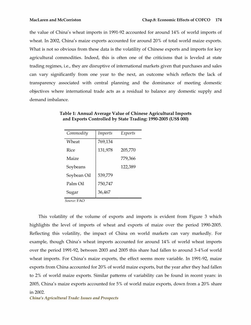
MacLaren and McCorriston Chap.8: Economic Effects of COFCO 174
China's Agricultural Trade: Issues and Prospects
the value of China‘s wheat imports in 1991-92 accounted for around 14% of world imports of
wheat. In 2002, China‘s maize exports accounted for around 20% of total world maize exports.
What is not so obvious from these data is the volatility of Chinese exports and imports for key
agricultural commodities. Indeed, this is often one of the criticisms that is leveled at state
trading regimes, i.e., they are disruptive of international markets given that purchases and sales
can vary significantly from one year to the next, an outcome which reflects the lack of
transparency associated with central planning and the dominance of meeting domestic
objectives where international trade acts as a residual to balance any domestic supply and
demand imbalance.
Table 1: Annual Average Value of Chinese Agricultural Imports
and Exports Controlled by State Trading: 1990-2005 (US$ 000)
Commodity Imports Exports
Wheat 769,134
Rice 131,978 205,770
Maize 779,366
Soybeans 122,389
Soybean Oil 539,779
Palm Oil 750,747
Sugar 36,467
Source: FAO
This volatility of the volume of exports and imports is evident from Figure 3 which
highlights the level of imports of wheat and exports of maize over the period 1990-2005.
Reflecting this volatility, the impact of China on world markets can vary markedly. For
example, though China‘s wheat imports accounted for around 14% of world wheat imports
over the period 1991-92, between 2003 and 2005 this share had fallen to around 3-4%of world
wheat imports. For China‘s maize exports, the effect seems more variable. In 1991-92, maize
exports from China accounted for 20% of world maize exports, but the year after they had fallen
to 2% of world maize exports. Similar patterns of variability can be found in recent years: in
2005, China‘s maize exports accounted for 5% of world maize exports, down from a 20% share
in 2002.

MacLaren and McCorriston Chap.8: Economic Effects of COFCO 175
China's Agricultural Trade: Issues and Prospects
Figure 3: China’s Wheat Imports and Maize Exports: 1990-2005 (US$ 000)
0
500
1000
1500
2000
2500
1990 1992 1994 1996 1998 2000 2002 2004
US$ m
Maize Exports
Wheat Imports
Given the dominant role played by COFCO in Chinese agricultural trade for major
commodities, it is of no surprise that state trading was an important issue in the negotiations
concerning China‘s accession to the WTO in the late 1990s. The intended outcome was to ensure
that the activities of state trading enterprises were consistent with GATT Article XVII, with the
Accession Protocol stating:
1. China shall ensure that import purchasing procedures of state trading enterprises are fully transparent, and in compliance with the WTO Agreement, and shall refrain from taking any measure to influence or direct state trading enterprises as to the quantity, value, or country of origin of goods purchased or sold, except in accordance with the WTO Agreement.
2. As part of China's notification under the GATT 1994 and the Understanding on the Interpretation of Article XVII of the GATT 1994, China shall also provide full information on the pricing mechanisms of its state trading enterprises for exported goods. (WTO, 2001, p. 5)
As part of the accession process, China agreed to relinquish part of the TRQs to non-state-
firms. The aim of this was to reduce the dominance of COFCO across various commodity
sectors, the specific mechanism being to allocate a specified share (but less than 100%) of the
TRQ to COFCO. The agreed shares of imports to be allocated are: 90% for wheat, 71–60%for
maize, 50%for rice, 42–10% for vegetable oils, 70% for sugar 33% for cotton and zero% for wool
(WTO, 2001, Schedule CLII, Part I, Section 1–B, p. 61-66). However, it should be noted that the
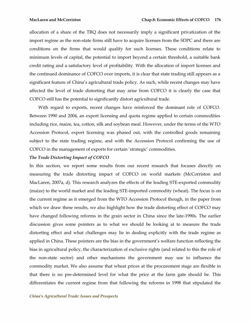
MacLaren and McCorriston Chap.8: Economic Effects of COFCO 176
China's Agricultural Trade: Issues and Prospects
allocation of a share of the TRQ does not necessarily imply a significant privatization of the
import regime as the non-state firms still have to acquire licenses from the SDPC and there are
conditions on the firms that would qualify for such licenses. These conditions relate to
minimum levels of capital, the potential to import beyond a certain threshold, a suitable bank
credit rating and a satisfactory level of profitability. With the allocation of import licenses and
the continued dominance of COFCO over imports, it is clear that state trading still appears as a
significant feature of China‘s agricultural trade policy. As such, while recent changes may have
affected the level of trade distorting that may arise from COFCO it is clearly the case that
COFCO still has the potential to significantly distort agricultural trade.
With regard to exports, recent changes have reinforced the dominant role of COFCO.
Between 1990 and 2004, an export licensing and quota regime applied to certain commodities
including rice, maize, tea, cotton, silk and soybean meal. However, under the terms of the WTO
Accession Protocol, export licensing was phased out, with the controlled goods remaining
subject to the state trading regime, and with the Accession Protocol confirming the use of
COFCO in the management of exports for certain ‗strategic‘ commodities.
The Trade Distorting Impact of COFCO
In this section, we report some results from our recent research that focuses directly on
measuring the trade distorting impact of COFCO on world markets (McCorriston and
MacLaren, 2007a, d). This research analyzes the effects of the leading STE-exported commodity
(maize) to the world market and the leading STE-imported commodity (wheat). The focus is on
the current regime as it emerged from the WTO Accession Protocol though, in the paper from
which we draw these results, we also highlight how the trade distorting effect of COFCO may
have changed following reforms in the grain sector in China since the late-1990s. The earlier
discussion gives some pointers as to what we should be looking at to measure the trade
distorting effect and what challenges may lie in dealing explicitly with the trade regime as
applied in China. These pointers are the bias in the government‘s welfare function reflecting the
bias in agricultural policy, the characterization of exclusive rights (and related to this the role of
the non-state sector) and other mechanisms the government may use to influence the
commodity market. We also assume that wheat prices at the procurement stage are flexible in
that there is no pre-determined level for what the price at the farm gate should be. This
differentiates the current regime from that following the reforms in 1998 that stipulated the

MacLaren and McCorriston Chap.8: Economic Effects of COFCO 177
China's Agricultural Trade: Issues and Prospects
price that farmers would receive for grain and a quota to be delivered to the state sector via the
Grain Bureaus.
With respect to the bias of agricultural policy, it is of course difficult to attach a precise
weight or measure to this. As noted above, the use of state trading in China reflects a range of
objectives including food security, ensuring food supplies and stabilizing markets. However, it
appears that in recent years, the bias of agricultural policy in China has tilted towards favoring
producers. This is reflected in recent Producer Support Equivalent (PSE) measures for China. In
the mid-1990s, the aggregate PSE measures were negative reflecting a bias towards consumers;
more recently, the bias has switched to producers with the average PSE measure now positive.
However, for wheat the PSE (CSE) is negative (positive) though for maize, the PSE (CSE) is
positive (negative). Reflecting this, we assume a ‗mild‘ bias towards consumers (producers) for
the wheat (maize) sectors in the results we derive below.
Modeling the nature of exclusive rights and the role of the private sector poses some
challenges for addressing issues in the wheat sector. There are three aspects of this that need to
be considered. First, the reforms in the wheat marketing sector in recent years have allowed for
non-state enterprises to procure and distribute domestically produced wheat. Moreover, given
the nature of these enterprises, their objective function will likely differ from that of COFCO as,
not being explicit instruments of government policy, their interests will lie in maximizing
profits. Second, the mechanics of the TRQ system under the WTO Accession Protocol allocates a
share of the TRQ away from COFCO. As noted in the discussion above, to qualify for an import
license, the enterprise has to fulfill certain criteria. This potentially differentiates them from non-
state enterprises in the domestic market that will not qualify or not be allocated a license for
whatever reason. To capture this, we differentiate these licensed firms (which can still procure
from the domestic market) from those that can only participate in the domestic but not import
market. Therefore, in our set-up, we have three types of enterprises that co-exist: the non-state
domestic enterprises; the licensed firms that can procure from the domestic market and imports;
and the state sector that plays a role in the domestic market and via COFCO which acts as the
agent in procuring and distributing imports.
However, there is a third issue which we attempt to incorporate, namely, the
administration of import licenses in the presence of COFCO and the hierarchical nature of
decision making in China. One aspect of the hierarchical decision-making is that the State

MacLaren and McCorriston Chap.8: Economic Effects of COFCO 178
China's Agricultural Trade: Issues and Prospects
Development and Planning Council, determines jointly the level of imports and domestic
procurement. This captures the idea that COFCO‘s purchases are not independent of the
decisions made by the SDPC in determining requirements in the domestic market. When it
comes to the import licenses of the non-state firms, once given a license, they freely determine
how much to import to maximize profits which is contingent on their decisions in the domestic
wheat sector. The alternative to this scenario is one involving a more subtle way of modeling
the imports of non-state firms. Specifically, since the state allocates these licenses and as the
share of the TRQ that is specifically allocated between the non-state enterprises and COFCO has
already been determined, the non-state firms are not free to import how much they choose, as
they have already been allocated some proportion of the total quota and therefore related to
what the SDPC would determine. As such, if they import, the license determines how much
they will import and the profit maximizing decision in the domestic market takes the import
allocation as given. As we show below, characterizing the decision process in this way has an
important effect on determining the trade distorting effect of COFCO.
Details of the data used to calibrate the model and the assumptions regarding the
competitiveness of the underlying benchmark can be found in McCorriston and MacLaren
(2007d). In brief, the model was calibrated using wheat sector data for 2005/06. We assumed
that China has some degree of market power in procuring imports, i.e., it is a large country in
the international wheat market. Domestic and imported wheat are assumed to be relatively
homogeneous and that the underlying private sector benchmark was fairly but not ‗too‘
competitive.10
Table 2 reports the results for the potential trade distorting effect of COFCO in the world
wheat market. The two cases reported reflect the different assumptions about the decision-
making process and the impact that this has on the imports of the licensed enterprises. It is clear
that, whatever assumption is used, the tariff equivalent effect of COFCO is negative, reporting
an import subsidy equivalent as high as US$29 per tonne in the restricted case, which is around
14% of the world price for that year. The non-restricted case reports a lower import subsidy
equivalent: although the licensed firms can potentially import more under this ‗unrestricted‘
regime, total imports are lower as, in this case, we have to account for the strategic interaction
between COFCO and the licensed firms (and also between the latter) that would not otherwise
10 In the framework we use, all these assumptions can be readily varied. The sensitivity of the results to these assumptions can be found in McCorriston and MacLaren (2007d).

MacLaren and McCorriston Chap.8: Economic Effects of COFCO 179
China's Agricultural Trade: Issues and Prospects
exist in the ‗restricted‘ regime. Varying the assumptions used in calibrating the model does not
change the overall picture even though it changes the magnitude of the tariff equivalent. More
important is the assumption of the bias in government policy. Reflecting the PSE/CSE values
for China in the wheat sector, we have assumed a bias towards consumers. However, switching
the bias towards producers and away from consumers would result in a positive tariff
equivalent equal to US$316 per tonne. The overall conclusion is that COFCO distorts market
access, the magnitude of this effect is potentially significant, and the impact of COFCO on the
world wheat market reflects the bias in government policies.
Table 2: Trade Distorting Impact of COFCO in the Wheat Market
Tariff Equivalent Effect -restricted case -$US 28.9/tonne
-non-restricted case $US17.8/tonne China: net welfare effect1 -restricted case 0.12 -non-restricted case 0.43 Exporters‘ welfare1 -restricted case 16.1 -non-restricted case 9.8 1 Percentage change from private firm benchmark
All trade distortions affect welfare and the same is true of state trading. Table 2 therefore
reports the welfare effects associated with the trade distorting effect of COFCO. There are two
main results to note. First, in the restricted case, net welfare for China is slightly increased (by
0.12%) compared with what would have arisen if COFCO did not exist. This increase reflects
the increase in consumer surplus which is associated with the increase in imports arising from
the import subsidy equivalent. In addition, reflecting the negative trade distorting effect and
therefore the increase in market access associated with it, welfare for exporters is higher (by
16%) compared with the private firm benchmark. Second, in the unrestricted case, net welfare
in China is higher by 0.43% and exporters' welfare higher by around 10% the latter reflecting

MacLaren and McCorriston Chap.8: Economic Effects of COFCO 180
China's Agricultural Trade: Issues and Prospects
the relatively lower negative tariff equivalent effect.11 Note that driving the sign of the trade
distorting effect and therefore the implications for welfare in China and that of third country
exporters is the bias of government policies. If the bias of these policies were to change to favor
producers, the trade distorting effect would change sign resulting in a positive trade distorting
effect, restricted market access, lower welfare for exporters and net welfare benefits for China.
Of course, as with all trade instruments, the net welfare effects hide the internal re-distributive
effects which are substantial.12
Table 3: Trade Distorting Effect of COFCO in the Maize Market
Subsidy equivalent effect US$14.2/tonne China: net welfare effect1 -5.4 Competing exporters‘ welfare1 -0.3 Importers‘ welfare1 23.6
1 Percentage change from private firm benchmark
Finally, Table 3 reports results from McCorriston and MacLaren (2007a) relating to
COFCO's presence in the world maize market. Reflecting the positive (negative) PSE (CSE)
measures in the Chinese maize sector, we assume a bias in the welfare towards producers.
Resulting from this, the subsidy equivalent is positive amounting to around 13% of the world
price. This is clearly a significant subsidy equivalent effect which affects competing exporters.
Reflecting this, their welfare falls by –0.3% while net welfare for China also falls by –5.4%.
Importing countries would nevertheless benefit from this positive subsidy equivalent, welfare
in the importing countries rising by around 23%.13
Taken together, these results relating to the use of state trading in China confirm that in
both import and export markets COFCO has a significant potential to distort trade. However,
the extent to which it does so and, in turn, the impact this has on welfare in China and in the
11 Note that the net welfare effects for China include the re-distribution between producers, marketing firms‘ profits and consumers while, for the exporting countries affected by the tariff equivalent, we assume no domestic consumption. 12 We report a larger array of results including the effects on producers, consumers and profits in McCorriston and MacLaren (2007d). 13 Again, this relatively large figure reflects no net domestic transfers where the gains to one group are diluted by the losses to another.
MacLaren and McCorriston Chap.8: Economic Effects of COFCO 181
China's Agricultural Trade: Issues and Prospects
rest of the world will reflect China‘s priorities with respect to the direction of its agricultural
policy objectives and the role that China plays in world markets. The hierarchical nature of
decision-making in China also has an important bearing in addressing the impact of COFCO on
world markets.
Finally, there are three important caveats to bear in mind when reviewing the results. First,
these results are indicative of the potential of COFCO to distort agricultural markets, rather
than being definitive. But the framework does highlight the factors that will determine these
effects. Second, the evidence from the OECD data on PSE measures suggests the bias in Chinese
agricultural policy has been changing in recent years. Given that the bias in the welfare function
is one of the key determinants of the impact of state trading, on-going developments in the
direction of policy objectives of the central government in China will have an important bearing
on the effect of COFCO on international markets. Finally, as is evident from Figure 3, China‘s
imports and exports from the world market are highly variable between years, reflecting among
other factors variability in domestic supply and demand imbalance. As such, one should expect
the potential impact of COFCO on world markets to also vary significantly from year to year.
Summary and Conclusions
The use of state trading in China in the form of COFCO has been a key feature of the
agricultural policy landscape in China for many years and as such is an important instrument
for the Chinese government in managing commodity markets and meeting its overall
objectives. Given the prevalence of state trading and the impact China can have on world
markets, it was of no surprise that the use of state trading was an important issue in China‘s
accession negotiations to the WTO. State trading nevertheless persists for key agricultural
commodities and applies to both imports and exports. Despite attempts in the WTO Accession
Protocol to limit (or diminish) the influence of state trading, COFCO still has significant
potential to control both imports and exports of several commodities.
In general, there is an absence of theoretical work that formally addresses the impact of
STEs on world markets. In this paper, we have drawn on some of our recent research to
highlight the factors that are likely to influence the effects that STEs have on world markets. We
have recently extended this body of research to deal with some of the explicit issues that arise
with respect to COFCO including aspects that specifically relate to the WTO Accession Protocol.
Our results confirm more casual expectations that COFCO does have the potential to distort
MacLaren and McCorriston Chap.8: Economic Effects of COFCO 182
China's Agricultural Trade: Issues and Prospects
world markets and, in turn, welfare for both China and other countries. In large part, the sign of
this trade distorting effect will reflect the overall bias in Chinese agricultural policy towards
producers and consumers as well as the terms of trade effects that arise due to China‘s size on
commodity markets. In sum, the manipulation of market structure via the use of state trading is
just another instrument of government policy, albeit one which requires a different focus to
measure the trade distorting and welfare effects that arise from it. Nevertheless, the impact of
state trading enterprises on trade is at least as significant, if not more so, than that of the more
obvious policy instruments.
References
ABARE . Agriculture in China: Developments and Significance for Australia. Research Report No.
06.2 (March 2006). Canberra: ABARE Lloyd, P. (1982) ―State Trading and the Theory of International Trade.‖ In State Trading in
International Markets, M.M. Kostecki (ed.). London: Macmillan Press (1982). McCorriston, S. and D. MacLaren. “The Trade-Distorting Impact of State Trading Enterprises in
Importing Countries.‖ European Economic Review 49(2005a): 1693-1715. McCorriston, S. and D. MacLaren. ―Single-Desk State Trading Exporters.‖ European Journal of
Political Economy 21(2005b): 503-524. McCorriston, S. and D. MacLaren. ―Do State Trading Exporters Distort Trade?‖ European
Economic Review 51(2007a): 225-246. McCorriston, S. and D. MacLaren. ―De-Regulation as (Welfare Reducing) Trade Reform: The
Case of the Australian Wheat Board.‖ American Journal of Agricultural Economics 89(2007b): 637-650.
McCorriston, S. and D. MacLaren. ―(Partial) De-Regulation of State Trading Importers.‖ Mimeo (2007c).
McCorriston, S. and D. MacLaren. ―Not So Liberal Trade Reform: State Trading and China‘s Accession to the WTO.‖ Mimeo (2007d).
Meade, J.E. Trade and Welfare. Oxford University Press: Oxford (1955). WTO. The Results of the Uruguay Round of Multilateral Trade Negotiations: The Legal Texts. Geneva:
The World Trade Organization (1995). WTO. Accession of the People’s Republic of China, Decision of 10 November, 2001. WT/L/432.
Geneva: World Trade Organization (2001).
Cai et al. Chap.9: The Lewisian Turning Point 183
China's Agricultural Trade: Issues and Prospects
Chapter 9:
Wage Increases, Labor Market Integration, and the Lewisian Turning Point: Evidence from Migrant Workers
FANG CAI1
YANG DU1
CHANGBAO ZHAO2
1 Institute of Population Studies and Labor Economics, Chinese Academy of Social Sciences
2 Research Center of Rural Economy, Ministry of Agriculture

Cai et al. Chap.9: The Lewisian Turning Point 184
China's Agricultural Trade: Issues and Prospects
Chapter 9:
Wage Increases, Labor Market Integration, and the Lewisian Turning
Point: Evidence from Migrant Workers*
Introduction
Development and integration of labor markets are key components that indicate the move
towards a market system. China‘s transition from an administered labor system to a labor
market is unique, not only because it is the largest economy in the world to experience such a
process, but because it has adopted a typically Chinese style of gradual change. Three elements
of China‘s labor market integration are important. First, it has been carried out with an
emphasis on incremental reforms, while not entirely negating the importance of shock reform.
Second, economic globalization has stimulated the process of labor market integration. Third,
the move towards a labor market parallels the transformation from a dual economy to one that
is integrated.
For a long time, China has been perceived as being a dual economy, evidenced by
unlimited labor supply. Thanks to low labor costs, labor-intensive industries have grown up
quickly, which has earned China the title of ―factory to the world‖. With fast growth in non-
agricultural sectors, the rural labor force has served as a source of labor to support
industrialization. However, a new trend has arisen in recent years, challenging the inherent idea
of an unlimited labor supply in China. Labor shortages are widely reported in various regions,
with some debate about whether China has entered an era of limited labor supply.
Mass rural-to-urban migration flows have brought about changes in the labor market. First,
rural migration workers have become an important component in urban labor markets and a
factor contributing to labor market integration. According to statistics from the National Bureau
of Statistics, more than 130 million migrants worked in urban areas in 2006, and labor mobility
encourages information flows across regions and economic sectors and leads to labor market
integration. Second, previously stagnant wages for migrant workers have started increasing. As
a result of large migration flows, non-agricultural sectors have soaked up the available labor in
*The authors would like to thank Wu Zhigang for assistance in processing data.
Cai et al. Chap.9: The Lewisian Turning Point 185
China's Agricultural Trade: Issues and Prospects
rural areas, in particular, those who are young and well-educated. For that reason, employers
that demand new participants have had to raise wage offers in order to attract workers. That is
why there have been significant wage changes for migrant workers in recent years. Finally,
faced with a Lewisian turning point, China needs to change the direction of its labor market
policies. For example, China ought to give up those temporary instruments designed to
suppress labor supply, widely used when labor market dislocation took place in urban areas in
the 1990s.
In this chapter, labor market reform and labor mobility of migration workers will be
discussed, followed by an analysis of the pattern of wage changes of migrant workers in recent
years, which provides some evidence for a Lewisian turning point. Then the results of using
regression-based inequality decomposition are used to disentangle the individual characteristics
that affect wage variations, as well as the contribution of regional factors to wage inequality.
Evidence of regional wage convergence suggests that the labor market has become more
integrated in recent years.
Employment Reform and Labor Mobility
Like related institutional arrangements in China, labor policy under the planned system
resulted in two kinds of inefficiencies. First, the inherent lack of labor supervision and lack of an
incentive mechanism in the micro-management system led to low technical efficiency. Second,
the distorted allocation of labor, capital, and other resources between regions and sectors led to
low allocative efficiency. Accordingly, the subsequent incentive mechanism, and allocation
system reforms have improved technical and allocative efficiencies, and have become dominant
drivers of the high economic growth that has occurred during the post-reform period in China.
Changes in labor policy have played an important role during the whole process of reform,
contributing directly and indirectly to efficiency improvements.
China‘s gradual institutional changes have embodied two initiatives: a ―bottom-up‖
initiative and one that is ―top-down.‖ In the first case, once the political climate at large began
to change, producers who had previously suffered under the strict constraints of the old system,
and who could see the potential gains from the new system, actively encouraged reform. In the
second case, government examined the way in which the old institutions constrained
productivity, as well as the potential efficiency gains of new institutions, and after comparing
the costs and benefits of institutional change, it implemented policy reform on its own initiative.

Cai et al. Chap.9: The Lewisian Turning Point 186
China's Agricultural Trade: Issues and Prospects
The formation of labor markets in China came about similarly: the implementation of the
Household Responsibility System (HRS) meant that rural laborers were released from
engagement in the agricultural sector, and began migrating between villages and towns and
even across provinces. When a large number of migrant workers found jobs in urban sectors,
competition began between the state-owned sector and the non-state sector, forcing the former
to consider reforming the labor recruitment and hiring system. Partly as a response to this, and
partly because of the problem of low productivity, the government gradually relaxed its labor
policy. Since policymaking is, after all, a function of government and since it is a decisive force
in the liberalization of a labor market, the intention and the extent of reforms of government
labor allocation policies have determined and are determining the pace of labor market
formation.
In the process of institutional change, playing the role of supplier of institutions,
government is also a rational agent, taking into consideration economic and political aspects in
its decision-making. Whether or not to abolish an old policy while adopting a new one depends,
not only on the revealed efficiency gains, but must also be restrained by the costs and benefits of
this change. The terms ―cost‖ and ―benefit‖ here refers to economic and political effects.
Increasingly deeper reform brings about an expansion in the market as a principal force behind
resource allocation. To avert conflict between traditional government methods and market
forces, the Chinese government has duly adjusted its policies in response to market
development. Labor policy reforms have depended directly on the overall extent of market
maturity. While on the one hand, the development of the labor market makes up a key part of
the economic reform as a whole, on the other, it goes only as far as the reach of overall reform.
As discussed above, during the process of labor policy reform, the Chinese government
and other players interacted with one another by following the rationale of political economy.
As part of marketization, the reform of labor policy and the implementation of other related
reforms have been/are being conditioned on each other. Following this framework, the
deregulation of labor mobility has been embodied mainly in rural-to-urban migration,
characterized as gradual abolition of the hukou system.
Since the beginning of the 21st century, the gradual reform of hukou has been characterized
by a bottom-up process. That is, relaxation of hukou control began in small towns and gradually
extended to medium-sized towns and big cities. The hukou system reform in more than 20,000
Cai et al. Chap.9: The Lewisian Turning Point 187
China's Agricultural Trade: Issues and Prospects
small towns was characterized by ‗minimum criteria and complete opening-up‘. In 2001, after
years of experimentation in some regions, the Ministry of Public Security initiated action to
reform the hukou system in small towns. In most small towns, the minimum requirement for
receiving local hukou is that the applicants must have a permanent source of legal housing in the
locality. This was considered one of the greatest and most complete steps in hukou reform since
the system was formed in 1958. Hukou relaxation in some medium-sized cities, and even in
some larger cities and provincial capitals, has been characterized by ‗abolishing quotas and
conditioned entry‘. The threshold for settling in those cities with hukou status has been lowered
substantially. This approach to reforming the hukou system meets the needs of a maturing labor
market(s) and corresponds with gradualism. Hukou relaxation, especially in large cities such as
Beijing and Shanghai has been characterized by ‗lifting up the threshold and opening the gate‘.
These cities have actively encouraged the arrival of intellectuals and professionals while
imposing strict criteria of entry on ordinary migrant workers. In short, lifting the threshold
means narrowing the doorway. By comparison, hukou reform in those cities has not made much
progress.
The reforms in urban employment, social security, and welfare provision have created an
institutional climate for rural-to-urban migration. Such reforms include the expansion of urban
non-state sectors, the removal of rationing, the privatization of the housing distribution system,
and changes in employment policies and the social security system. These reforms have
reduced the costs of migrating to, working, and living, in cities. In the late-1990s, while the
urban employment ‗iron rice-bowl‘ was broken, rural workers began to enter the urban labor
market on a massive scale. It is becoming more common and much easier for rural laborers to
seek work and live in cities, even though the hukou system still functions. In short, labor
mobility motivated by reforms to the hukou system, and other institutions deterring migration,
has not only been an important part of economic development; it has also been and is a
significant part of the process of transition towards market forces. This transition has been
conditioned on the reforms in a much wider sphere. In this respect, the allocation of the labor
force across sectors and among regions is based increasingly on market forces. The
characteristics of migration in transitional China reflect that of marketization as a whole. The
procedure of labor market reforms in both rural and urban areas is summarized in Table 1.

Cai et al. Chap.9: The Lewisian Turning Point 188
China's Agricultural Trade: Issues and Prospects
Table 1: Labor Market Reforms in China
Time Rural Labor Market Urban Labor Market
Early 1980s Household Responsibility System (HRS) released laborers from agriculture, and Township and Village Enterprises (TVEs) reallocated them
To deal with the returned sent-down youth and new entrants of job market, three channels of employment combined
Late 1980s
Allowance of long distance trading of agricultural products; legitimizing of city work for farmers by bringing staple food for city stay
Reforms for permanent workers of State-Owned Enterprises (SOEs) by contracting and internal reallocation
Early 1990s
Migration tide, relaxation of hukou system – government‘s selling blue stamp of local hukou
Staffs and workers of SOEs and government departments jumping into the sea; abolition of rationing
Late 1990s
Mass migration, three ways of reforming hukou system from small towns to large cities
Breaking of iron-rice-bowl and rebuilding the social security system in the labor market shock period
Since this Century
Local autonomy for reforming hukou system; government‘s efforts in improving migration conditions
Further development of labor market characterized by diversification and informalization of employment; pilot programs of social security system

Cai et al. Chap.9: The Lewisian Turning Point 189
China's Agricultural Trade: Issues and Prospects
Due to the dual economic system implemented in China, there is significant segmentation
between rural and urban labor markets. The two markets have different levels of regulation,
leading to migrant and local workers being employed in two separate labor markets within the
same city. Governments tend to have less regulation for migrant workers, protecting them less
than local workers. For this reason, employment and wage formation for migrant workers are
determined mainly by market forces. Since the mid-1980s, migrant workers have been the major
component of labor flows between urban and rural areas and across regions. This group of
workers can be defined as those whose behavior was the first to be marketized in China. The
following features of migrant workers, reflects the mechanism of labor market integration
across regions.
First, as already mentioned, migrant workers have become a major component of the urban
labor market. Rural-to-urban migration began in the 1980s, and since then migration has
continued to increase. On the one hand, this has been because a fast-growing economy creates
increasing labor demands in non-agricultural sectors; on the other hand, the urban labor market
tends to be friendlier to migrant workers. Since China‘s entry into the World Trade
Organization (WTO), the labor-intensive industries in which China has a comparative
advantage have grown, intensifying the demand for the agricultural labor force. As
demonstrated in Table 2, migrant workers in the urban labor market provide an important
human resource that supports rapid economic growth. In 2006, the ratio of migrant workers to
urban employees was 46.7%. Therefore, regional labor market integration can be understood by
examining the employment and wage levels of migrant workers.
Table 2: Number of Migrant Workers in the Urban Labor Market
Year (1)Migrant workers
(thousand) (2) Urban employment
(thousand) Ratio of 1/2
(%)
2000 78,490 212,740 36.9 2001 83,990 239,400 35.1 2002 104,700 247,800 42.3 2003 113,900 256,390 44.4 2004 118,230 264,760 44.7 2005 125,780 273,310 46.0 2006 132,120 283,100 46.7
Sources: The size of the migrant workforce from National Bureau Statistics (NBS), Yearbook of Rural Household Survey (various years); data on urban employment are from NBS, Yearbook of Labor Statistics in China (various years)

Cai et al. Chap.9: The Lewisian Turning Point 190
China's Agricultural Trade: Issues and Prospects
China’s Lewisian Turning Point
As a result of China‘s economic growth and demographic change, the country is approaching a
turning point at which labor shortages and wage increases occur. As part of this process, the
speed of labor market integration will increase as well. Through integration into the global
division of labor, China‘s labor-intensive manufacturing sector has boomed, and world-wide
employment opportunities have been seized. As a result, more than 100 million rural laborers
have migrated to urban jobs, and laid-off and unemployed workers have been re-employed in
an economy with high growth rates. With economic development, the pattern of factor
endowments in China is being restructured, implying the coming of a historical turning point.
According to population predictions, the desirable population structure that has brought
about a demographic dividend in the past three decades will disappear within the next decade.
At this point, the dependant population ratio (the ratio of the population aged younger than 16
and older than 64 with respect to those aged between 16 and 64) will stop decreasing and begin
increasing. When comparing the growth rates of labor forces in other countries, it becomes clear
that within two decades China will have no advantage in labor supply (United Nations, 2005).
In fact, the outcome of demographic transition has already appeared in the labor market where
the coming Lewisian turning point is characterized by the following two stylized facts. The first
is quantity adjustment evidenced by labor shortage and exhaustion of the supply of young
workers. The second is price adjustment evidenced by rising wages and wage convergence
among various groups of workers.
In 2003, a shortage of migrant workers was first reported in coastal areas, which are the
most developed regions in China. At that time, the shortage was not taken seriously because the
common understanding of the issue was that it was a transitory and structural phenomenon
that would disappear with labor market adjustment. However, shortages have affected other
regions since then, indicating that labor shortages are a long-term issue rather than a temporary
one. This is explained by the demographic changes and workforce reallocation in rural China.
In 2005, out of a rural labor force estimated at 485 million, approximately 200 million changed
jobs by either leaving their home townships or shifting to non-agricultural sectors. The
agricultural sector requires about 178 million workers, creating a surplus of about 100 million
workers, half of whom are over 40 years old. This fact is significantly different from what

Cai et al. Chap.9: The Lewisian Turning Point 191
China's Agricultural Trade: Issues and Prospects
scholars have long believed, and it marks the coming of a Lewisian turning point (Cai and
Wang, 2008).
In addition to quantity response in the labor market, wage increases are also significant.
According to surveys conducted by the Ministry of Agriculture, from 2004 to 2006, annual
growth rates of monthly earnings for migrant workers was 2.8%, 6.5%, and 11.5%, respectively
(Cai, 2007). The Ministry of Labor and Social Security reported a growth rate of 17.9% in
monthly earnings for migration workers in 2006 (Cai, 2007).
Looking at a more detailed breakdown of wage changes, the trend of wage dynamics
among various groups also indicates the coming Lewisian turning point. In Figure 1, the wage
changes by education attainment in the past few years are displayed. In 2003, the wage gap
between skilled and unskilled workers was quite substantial and converged in the following
years. Because the shortage was for low-skilled workers who had accomplished junior high
school, this group of workers had the most significant and stable wage increase, the annual
growth rate being 9%. Similarly, for workers whose education attainments were primary
schooling or below, the annual growth rate was 8.1%. Wage increases of low-skilled workers,
implies that labor shortages are not a transitory or structural phenomenon but are instead
caused by an imbalance between aggregate demand for and supply of labor.
Figure 1: Wage Trend of Workers by Education Attainment
Source: Authors‘ calculation from Research Center of Rural Economy (RCRE) data
924
888
1037
687
728
787
853 794
756 728
877 878
1094 1015
1098
1116
600
700
800
900
1000
1100
1200
2003 2004 2005 2006
Prim. and below Jr. High School Sr. High School Above Sr.HS
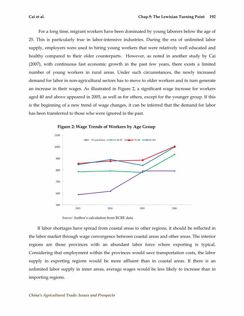
Cai et al. Chap.9: The Lewisian Turning Point 192
China's Agricultural Trade: Issues and Prospects
For a long time, migrant workers have been dominated by young laborers below the age of
25. This is particularly true in labor-intensive industries. During the era of unlimited labor
supply, employers were used to hiring young workers that were relatively well educated and
healthy compared to their older counterparts. However, as noted in another study by Cai
(2007), with continuous fast economic growth in the past few years, there exists a limited
number of young workers in rural areas. Under such circumstances, the newly increased
demand for labor in non-agricultural sectors has to move to older workers and in turn generate
an increase in their wages. As illustrated in Figure 2, a significant wage increase for workers
aged 40 and above appeared in 2005, as well as for others, except for the younger group. If this
is the beginning of a new trend of wage changes, it can be inferred that the demand for labor
has been transferred to those who were ignored in the past.
Figure 2: Wage Trends of Workers by Age Group
Source: Author‘s calculation from RCRE data
If labor shortages have spread from coastal areas to other regions, it should be reflected in
the labor market through wage convergence between coastal areas and other areas. The interior
regions are those provinces with an abundant labor force where exporting is typical.
Considering that employment within the provinces would save transportation costs, the labor
supply in exporting regions would be more affluent than in coastal areas. If there is an
unlimited labor supply in inner areas, average wages would be less likely to increase than in
importing regions.
500
600
700
800
900
1000
1100
2003 2004 2005 2006
25 and below 26-30 31-40 40+

Cai et al. Chap.9: The Lewisian Turning Point 193
China's Agricultural Trade: Issues and Prospects
However, as depicted in Figure 3, average wages in central and western China have also
grown steadily. Additionally, the wage gap between coastal areas and interior regions has been
shrinking in the past few years. In 2003, the ratio of average wages for migrants in interior areas
to those in coastal areas was 0.75 while the ratio went up to 0.86 in 2006. The disappearing gap
not only indicates a more integrated labor market among regions, but reflects the fact that labor
in exporting regions has been put to good use.
Figure 3: Wage Trends of Workers by Region
Source: Authors‘ calculation from RCRE data
Wage Convergence of Migrants
In a previous study, aggregated wage data on sub-sectors in manufacturing were used to
analyze the deviation of average wages by province and found that markets were integrated
between regions (Cai and Du, 2004). Although industrial factors that affect wages were
controlled for, the study could not reflect the impact of purely regional effects since, with
aggregated data, it is impossible to control for individual characteristics. Hence, data at a micro
level can be used, and it is expected that the impact of regional factors on labor market
integration since China‘s WTO entry can be observed.
Data
Data in this chapter were collected by the Research Center of Rural Economy (RCRE), in the
Ministry of Agriculture. In the past decade, the center has consistently surveyed 20,000
households, distributed throughout 300 villages. In each household, a basic form was filled out
0
200
400
600
800
1000
1200
2003 2004 2005 2006
other regions coastal region

Cai et al. Chap.9: The Lewisian Turning Point 194
China's Agricultural Trade: Issues and Prospects
that included information such as level of education, age, gender, and health status. Since 2003,
a complementary labor survey has been done in order to gain more information about labor
migration. From the individuals surveyed, information about the destinations to which
migrants go to work can be collected. Combining the household and individual data,
information on individual characteristics, wages, and working places can be obtained in order
to begin to understand the impacts that geographic factors have on wage inequality.
Inequality Measures and Decomposition: Regional Effects
In general, the disparities of individual earnings can be attributed to factors in three categories.
The first is individual characteristics, including human capital and demographic characteristics
such as age and gender. The second is industrial and occupational features. Even in
industrialized countries, where labor markets function very well, earning disparities between
industries exist and persist: workers in different industries with similar individual
characteristics can earn different incomes. The third factor is regional. Regional disparities do
not easily disappear when labor mobility between regions does not occur. The market
mechanism plays an active role in the market for migrant workers, and the industrial and
occupational distribution of migrant workers concentrates in a few industries and occupations.
It is, therefore, plausible to explore the role of regional effects of market integration when
individual features of particular markets are controlled for.
Table 3: Income Inequality Measures: 2004-2006
2003 2004 2005 2006
Percentile ratios p90/p10 4.469 4.444 4.436 4.232 p90/p50 2.083 2.222 2.096 2.081 p10/p50 0.466 0.500 0.472 0.492 p75/p25 2.143 2.143 2.013 2.083
General entropy GE(-1) 0.299 0.285 0.236 0.232 GE(0) 0.240 0.226 0.192 0.189 Theil 0.270 0.246 0.204 0.196 GE(2) 0.436 0.377 0.282 0.258 Gini 0.374 0.360 0.334 0.332
Atkinson indices A(0.5) 0.119 0.110 0.093 0.091 A(1) 0.214 0.202 0.175 0.172 A(2) 0.374 0.363 0.321 0.317
Source: Authors‘ calculations
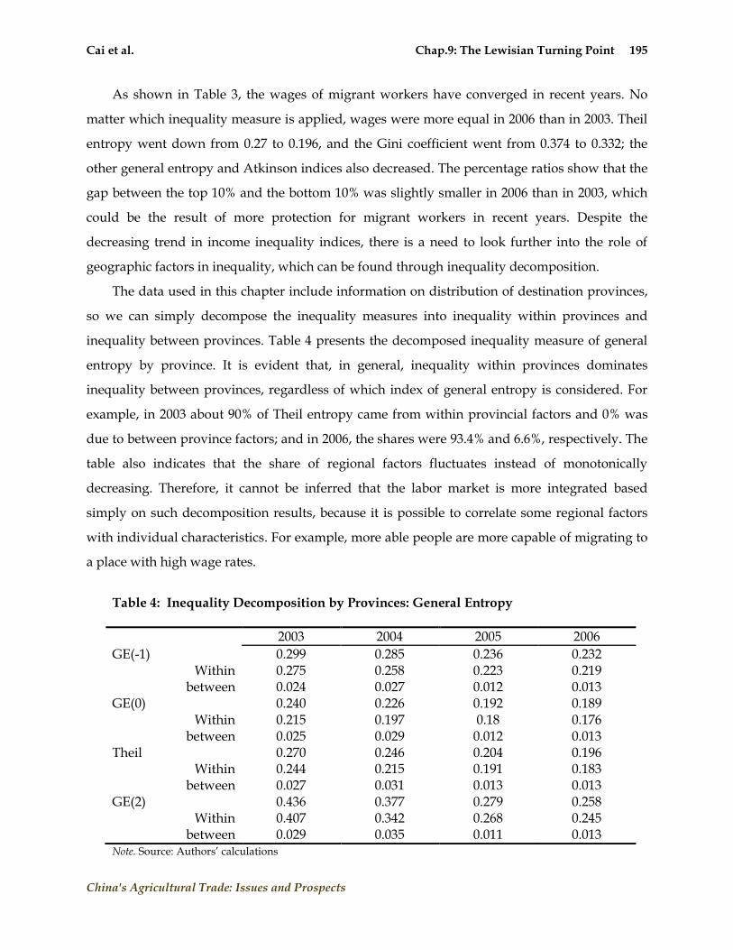
Cai et al. Chap.9: The Lewisian Turning Point 195
China's Agricultural Trade: Issues and Prospects
As shown in Table 3, the wages of migrant workers have converged in recent years. No
matter which inequality measure is applied, wages were more equal in 2006 than in 2003. Theil
entropy went down from 0.27 to 0.196, and the Gini coefficient went from 0.374 to 0.332; the
other general entropy and Atkinson indices also decreased. The percentage ratios show that the
gap between the top 10% and the bottom 10% was slightly smaller in 2006 than in 2003, which
could be the result of more protection for migrant workers in recent years. Despite the
decreasing trend in income inequality indices, there is a need to look further into the role of
geographic factors in inequality, which can be found through inequality decomposition.
The data used in this chapter include information on distribution of destination provinces,
so we can simply decompose the inequality measures into inequality within provinces and
inequality between provinces. Table 4 presents the decomposed inequality measure of general
entropy by province. It is evident that, in general, inequality within provinces dominates
inequality between provinces, regardless of which index of general entropy is considered. For
example, in 2003 about 90% of Theil entropy came from within provincial factors and 0% was
due to between province factors; and in 2006, the shares were 93.4% and 6.6%, respectively. The
table also indicates that the share of regional factors fluctuates instead of monotonically
decreasing. Therefore, it cannot be inferred that the labor market is more integrated based
simply on such decomposition results, because it is possible to correlate some regional factors
with individual characteristics. For example, more able people are more capable of migrating to
a place with high wage rates.
Table 4: Inequality Decomposition by Provinces: General Entropy
2003 2004 2005 2006
GE(-1) 0.299 0.285 0.236 0.232 Within 0.275 0.258 0.223 0.219
between 0.024 0.027 0.012 0.013 GE(0) 0.240 0.226 0.192 0.189
Within 0.215 0.197 0.18 0.176 between 0.025 0.029 0.012 0.013
Theil 0.270 0.246 0.204 0.196 Within 0.244 0.215 0.191 0.183
between 0.027 0.031 0.013 0.013 GE(2) 0.436 0.377 0.279 0.258
Within 0.407 0.342 0.268 0.245 between 0.029 0.035 0.011 0.013
Note. Source: Authors‘ calculations

Cai et al. Chap.9: The Lewisian Turning Point 196
China's Agricultural Trade: Issues and Prospects
Regression Based Decomposition
To further examine the components of income inequality, and following Morduch and Sicular
(2002), Theil entropy was decomposed, using the following linear earning regression model:
29
t t t t t t t t t t t t ti 0 1 i 2 i 3 i 4 i j j i
j=1
E = α +α edu +α sex +α age +α heath + β d + ε ,
where the left-hand side variable is monthly earnings of a migrant, and the first four right-hand
side variables are individual characteristics, including years of schooling, gender, age, and self-
reported health status. Except for an error term, the last two terms include the sum of provincial
dummies. Unlike typical earnings equations that use a log of wages as a dependent variable, for
the purpose of decomposing the inequality index, in this case Theil entropy, the advantage of a
semi-log equation is sacrificed, since the main goal in this research is to look at the role of
geographic factors in wage inequality instead of returns to human capital.
Table 5 presents some of the regression results on individual characteristics. The provincial
dummies were not included in order to save space, while the effects of specific provinces were
not of interest here. The regression results were generally consistent with traditional
predictions, i.e., educated, healthy, male, and aged labor has a relatively better economic
performance in the labor market.
Table 5: Regression Results of Linear Wage Equation: 2003-2006
2003 2004 2005 2006
Years of schooling 37.63 (3.08)
29.66 (3.17)
20.11 (3.27)
34.94 (2.71)
Gender (1= male) 197.44 (15.96)
197. 86 (15.56)
54.33 (15.81)
231.78 (13.84)
Age 10.41 (0.71)
10.02 (0.69)
6.93 (0.69)
9.35 (0.60)
Self-reported health Status
-59.97 (12.72)
-74.94 (12.70)
-17.37 (13.30)
-108.19 (11.21)
Provincial dummies yes yes yes yes
R2 (adj-R2) 0.13 (0.12)
0.15 (0.15)
0.061 (0.056)
0.12 (0.12)
No. of observations 8372 7986 6040 10094 Notes: 1. Standard errors in parentheses; 2. Health status is self-reported in five ranks, where one is healthier than five

Cai et al. Chap.9: The Lewisian Turning Point 197
China's Agricultural Trade: Issues and Prospects
Using the information on the right-hand side variables, it is possible to decompose Theil
entropy into regional effects, which are the sum of provincial effects, individual effects,
constants, and residuals, the results being presented in Table 6. The main interest in this chapter
is to look at the contribution of regional factors to inequality when individual characteristics are
controlled for. In 2003, 28% of wage inequality could be explained through regional factors,
while the share was 20.3% in 2006. A monotonic decreasing trend of regional inequality was
also found for the years following China‘s entry into the WTO entry. Although only a few
observations were available, due to a very short time-series, the first row of Table 6 shows that
regional labor markets have become integrated, at least for migrant workers.
Table 6: Theil Decomposition Based on Regression
Components of inequality 2003 2004 2005 2006
Theil Entropy 0.270 0.246 0.204 0.196
Regional factors (%) 28.08 26.10 22.84 20.31
Individual factors (%) -63.88 -52.92 -33.03 -44.49
Constant (%) -11.16 -26.22 -60.89 -41.06
Residual (%) 146.96 153.04 171.08 165.24
Total (%) 100 100 100 100 Source: Authors‘ calculations
Conclusion
By looking at wage changes in various dimensions, this chapter has explored evidence for a
coming Lewisian turning point in recent years. An analysis of the data for migrant workers
shows that the pattern of stagnant wages lasting for a decade has been broken. Meanwhile, the
pattern of wage changes supports the argument that China is drawing near to a Lewisian
turning point that is the result of fast economic growth and demographic transition.
Average wages among regions converged. The trend is indicated by both measurement of
inequality of wages and by inequality decomposition. Controlling for individual characteristics
that affect wages reveals that regional factors contributed less and less to total inequality of
wages. This suggests that the labor market is more and more integrated among regions. It is
evident that labor market reforms that lead to large flows of labor drive the process of labor
market integration.
Labor market reform is, however, far from complete. In addition, the coming Lewisian
turning point further challenges institutional reforms. Abolition of the various institutional

Cai et al. Chap.9: The Lewisian Turning Point 198
China's Agricultural Trade: Issues and Prospects
obstacles that hinder the development of a labor market will not only enhance migration flows,
it will make it a rational movement as well by helping to create the developmental climate and
job opportunities for labor mobility, which in turn will produce favorable conditions for the
abolition of the hukou system. The Chinese government, which has specific development goals
for the next two decades, should grasp every opportunity to push institutional reforms and to
encourage labor migration once its importance is fully realized.
References
Cai, F., and Y. Du. ―Labor Market Integration: Evidence from Wage Convergence in
Manufacturing.‖ China Update. Asia Pacific Press (2004). Cai, F., (ed.). The Coming Lewisian Turning Point and Its Policy Implications. Reports on China‘s
Population and Labor, No. 8 (2007). Beijing: Social Science Academic Press. (2007). Cai, F. and M. Wang. ―A Counterfactual Analysis on Unlimited Surplus Labor in Rural China.‖
China and World Economy 16(2008):51-65 Fan, G., and X. Wang. Indices of Marketisation in China: 2000. Beijing: Economic Science Press
(2001). Morduch, J. and T. Sicular. ―Rethinking Inequality Decomposition, with Evidence from
Rural China.‖ Economic Journal, 112(2002), 93-106. United Nations. World Population Prospects: The 2004 Revision. Department of Economic and
Social Affairs, Population Division. New York: United Nations (2005).

Kwieciński and von Tongeren Chap.10: Agricultural Policy Reforms in China 199
China's Agricultural Trade: Issues and Prospects
Chapter 10:
Quantitative Evaluation of Agricultural Policy Reforms in China: 1993-2005
ANDRZEJ KWIECIŃSKI
FRANK VON TONGEREN
OECD
Kwieciński and von Tongeren Chap.10: Agricultural Policy Reforms in China 200
China's Agricultural Trade: Issues and Prospects
Chapter 10:
Quantitative Evaluation of Agricultural Policy
Reforms in China: 1993-2005*
Introduction
This chapter discusses agricultural policy developments in China in qualitative terms and
provides a quantitative evaluation of policy reforms using the indicators of agricultural support
developed by the Organization for Economic Cooperation and Development (OECD), including
the Producer Support Estimate (PSE), Consumer Support Estimate (CSE), General Services
Support Estimate (GSSE) and Total Support Estimate (TSE). The method employed is fully
consistent with that applied to OECD members and other non-member countries, and hence
provides a sound basis for international comparison. Appendices provide an overview of the
OECD indicators of support and discuss specific methodological issues related to constructing
measures of support for the Chinese agricultural sector.
Background: Developments in the Agricultural Policy Framework
A wide range of government reports, statements, and planning documents underline that the
agricultural sector is viewed as very important for the Chinese economy in general and has a
high profile in policy making. The agricultural policy framework has been evolving in line with
China‘s gradual transition from a centrally planned economy towards a socialist market
economy since 1978. While the principal economic objective of creating a market-based
economy appears to have consistently underpinned agricultural policy trends, it is clear that the
reform process has not been completely smooth – occasionally, reforms appear to have been set
aside in order to allow measures dealing with unforeseen events to be implemented. Like all
national governments, the Chinese leadership has a multi-faceted set of objectives and is faced
with the task of developing policies to be applied in an uncertain future. China‘s policy-
implementation process has been relatively flexible, in the sense that broadly-defined central
government policies have been implemented in a variety of ways, according to the capacity and
* This paper has been prepared with statistical and research support from Ms. Florence Mauclert from the same Directorate and draws heavily on OECD (2005; 2007). Background data and policy information were provided by Mr. Guoqiang Cheng, Deputy Director General in the Development Research Center of the State Council, Beijing, China, and by Mr. Xiande Li, professor in the Institute of Agricultural Economics, CAAS, Beijing, China.

Kwieciński and von Tongeren Chap.10: Agricultural Policy Reforms in China 201
China's Agricultural Trade: Issues and Prospects
needs of the sub-national government bodies responsible for policy implementation. The
following three sections focus on the evolution of agricultural policy objectives in China during
the period 1990-2005, on specific agricultural policy measures applied to achieve these
objectives, and on major policy initiatives for the future.
Agricultural Policy Objectives and their Evolution
In general, the reforms of agricultural policies and institutions were directed towards increasing
the role of markets. These reforms were further stimulated by WTO accession negotiations
started before 1990 and concluded at the end of 2001. However, changes in domestic
circumstances and in world market conditions led to reprioritizing of measures in order to
achieve the broad reform objectives. Moreover, further reforms to improve market institutions,
such as enforceable contracts, transparent information, and open bargaining among several
buyers and sellers, are still needed. Generally, the period 1990-2005 can be divided into two
sub-stages in terms of major priorities and types of measures implemented.
1990 to 1997: In this period, the principal agricultural policy objective was to increase
agricultural production, especially that of food grains, and to ensure food security. While the
central government was responsible for food security, important responsibility was devolved to
provincial governments, in particular within the Governor‘s Grain-Bag Responsibility System
(GGBRS) introduced in 1995. Under the GGBRS, provincial governments were to ensure the
availability of adequate supplies of food grains within provincial boundaries.
In line with the general economic policy initiative towards a market-oriented economy, this
period was also characterized by substantial deregulation of agricultural marketing and a
significant lessening of controls on the prices of agricultural products and on marketing
channels. However, while affordable food and stable prices were a policy objective throughout
this period, the objective became even more important in times of rising prices. For example,
following the liberalization of price controls in the early-1990s, inflation and rising food prices
in 1994 and 1995 resulted in a strengthening of government controls on prices and marketing
channels, followed again by a more gradual easing of regulation as prices stabilized.
1998 to 2005: This period was characterized by the adoption of policies supporting rural
income, representing a fundamental shift in the government‘s agricultural policy agenda. The
new policy direction was clearly spelled out in the document issued in 1998 by the Central
Committee of the Communist Party of China (CCCPC): ―The decision of the CPC Central

Kwieciński and von Tongeren Chap.10: Agricultural Policy Reforms in China 202
China's Agricultural Trade: Issues and Prospects
Committee on several major issues in agriculture and rural work.‖ The decision firmly made
the reduction of taxation of farmers and the improvement of their incomes as the guiding
principles of governmental policy until 2010. Agriculture began to be supported with the aim of
maintaining and improving the incomes of those dependent on farming. Food security
remained an important policy objective, while policies addressing food safety achieved a higher
profile in this period. As a result of growing urban affluence and relatively stable food prices,
food marketing and price controls became less important. The competitiveness of China‘s
agricultural production became a higher priority, in particular since China‘s WTO accession in
December 2001.
Major floods in the southern parts of China in 1998 gave renewed impetus to agro-
environmental policies. The floods highlighted land clearing and land usage practices which
contributed to the severity of the floods, prompting the ―grain for green‖ policy response (see
below). At the same time, continuing pressure on the main northern river systems increased
concerns over falling water tables and increasing desertification. These concerns underpin the
continuation of the Comprehensive Agricultural Development Program which provides
funding for soil and water conservation projects throughout China. Currently, improving
farmers‘ incomes and narrowing the urban–rural income gap are top priorities for the Chinese
government, while food security, or food-grain self sufficiency, still remains a principal policy
focus. High level policy documents, including the ―No. 1 Documents‖ between 2004 and 2007,
clearly outline these policy objectives, while proposing policy measures that include reduced
taxation of farmers, direct subsidies to grain farmers, measures to maintain farm land in
agricultural production, and measures to improve the adoption of technology in the agricultural
sector.
Key Agricultural Policy Measures and their Evolution
In accordance with the OECD approach, agricultural policy measures employed by the Chinese
government between 1995 and 2005 can be divided into producer support measures, general
services, and consumer support measures. In turn, producer support measures cover both
domestic and trade policy measures. This section provides a short overview of these measures
with a focus on those applied in the most recent years.
Kwieciński and von Tongeren Chap.10: Agricultural Policy Reforms in China 203
China's Agricultural Trade: Issues and Prospects
Domestic Policy Measures:
(i) State pricing: before 2004, state pricing accompanied by a state procurement system was
in place for major agricultural commodities. Since 2004, centrally set state pricing only applies
to tobacco, which remains under a state monopoly.
(ii) Minimum prices for grains: in May 2004, China allowed qualified non-state firms to buy
and sell grains on the open market. Private firms which meet certain criteria were also
permitted to engage in grain processing and storage activities. The government regulates the
grain market through national grain stocks, state trading enterprises (STEs) for foreign trade
transactions in grains, and minimum purchase prices. The minimum prices were first
announced in 2004 for early indica rice and japonica rice. In 2005 the coverage was extended to
include middle and late indica rice and again in 2006 to include wheat. Within the system,
domestic prices for grains are allowed to fluctuate relatively freely and the government
purchases for national stocks intensify when market prices fall below the minimum levels, as
happened in the summer of 2006.
(iii) Input subsidies: charges for water, electricity, and transport tend to be lower for
farmers, but the level of subsidy is difficult to assess, as the cost of provision is different across
various users. To lower prices of fertilizers, fertilizer producers have been given access to lower
priced inputs, such as electricity. In addition, export taxes, temporary exemptions from value
added tax (VAT), and caps on sales prices are occasionally used to curb rises in fertilizer prices.
Since 2002, farmers have been subsidized for the cost of purchasing improved quality soy seed.
In 2004 and 2005, this scheme was extended to include subsidies for purchasing improved seed
for production of wheat, corn, rice, and soybeans. The government also provides a small
subsidy for the purchase of farm machinery.
(iv) Credit subsidies: until the end of the 1990s, preferential loans were provided mostly to
state marketing organizations to fund the purchase and storage of key agricultural products. In
the 2000s, most of these programs were discontinued with the exception of grains. However, in
February 2006, the Agricultural Development Bank of China (ADBC), the so called ―policy
bank‖ implementing government programs, announced that commercial rates would also be
applied to the grain marketing enterprises. Preferential rates are now applied for loans targeting
rural population and poverty alleviation. In 2006, the rates were just above half the commercial
rates.

Kwieciński and von Tongeren Chap.10: Agricultural Policy Reforms in China 204
China's Agricultural Trade: Issues and Prospects
(v) Direct payments: initiated as a trial in 2002, and implemented nationally since 2004.
Farmers engaged in growing grains receive a direct budgetary financed subsidy based on the
current area of land they sow to rice, wheat, or corn. The rates may vary across provinces, but
on average they were at CNY 10 (USD 1.2) per mu (1/15 ha) in 2004 and since then increased to
CNY 12-14 per mu in 2007. While politically popular, the role of these subsidies in supporting
farm incomes is minor (Gale et al., 2005).
(vi) Payments for returning farmland to forests: also known as the ―grain for green‖
program, commenced in 1999. Farmers cultivating ecologically vulnerable land received a cash
subsidy and a grain allocation in kind for each mu they retired from agricultural production.
Subsidized seedlings were also available for afforestation. In 2004, payments in kind were
converted to cash equivalents. The period for which ―retired‖ land is subsidized is set at 2 years
for land returned to pasture, 5 years for land converted to ―economic‖ forests, and 8 years for
land converted to ―ecological‖ forests.
(vii) Agricultural taxes: until 2004, farmers were required to pay agricultural taxes either in
cash or in kind. In addition, they also paid various fees to local governments and collectives and
provided ―labor accumulation‖ for the construction of communal facilities. Agricultural tax
reform was initiated as a trial in 2000 and was phased in across rural China beginning in 2004.
In 2005, 28 provinces exempted farmers from agricultural taxes, and at the beginning of 2006 the
government announced that the tax was totally eliminated.
Trade Policy Measures:
(i) Tariffs: the simple average import tariff for agro-food products fell from 45% in 1992 to
15% in 2005, remaining at that level under the agreed terms of China‘s accession to the WTO.
(ii) VAT on imports: the rate for imports of agricultural goods is 13%, 4 percentage points
below the rate generally applied to other products. Depending on the market situation, VAT
exemptions have been applied sporadically to a wide range of agriculture-related imports, such
as grains, seeds, breeding animals, fertilizers and pesticides, some feed components, and cotton.
However, if there is a domestic oversupply of a given commodity, the VAT exemption on
imports is removed (WTO, 2006).
(iii) Tariff rate quotas (TRQs): first introduced for major grain and oilseed commodities in
1996. Under the terms of China‘s WTO accession, China can apply TRQs to wheat, maize, rice,
soybean oil, palm oil, rape oil, sugar, wool, wool tops, cotton, and chemical fertilizers. At the

Kwieciński and von Tongeren Chap.10: Agricultural Policy Reforms in China 205
China's Agricultural Trade: Issues and Prospects
beginning of 2006 the government announced the elimination of the TRQ on vegetable oils,
implementing tariff-only arrangements instead. China‘s TRQ system includes criteria for
allocating the import quotas to STEs and non-STEs.
(iv) State trading: dominating until the mid-1990s. Its role has been diminishing since then,
but it is still important for exports and imports of key commodities, in particular those covered
by TRQs. The continued use of state trading to import and export selected commodities allows
the government to influence their domestic prices.
(v) Export subsidies: prior to becoming a member of the WTO, China provided export
subsidies for maize and rice. In line with its WTO accession commitments, China is not allowed
to apply export subsidies.
(vi) Export taxes: under its WTO accession agreements, China maintains the right to apply
export taxes, but such taxes are not applied, with the exception of such commodities as raw
hides and skins of goats and, occasionally, fertilizers.
(vii) VAT rebates on exports: all exporters are entitled to a VAT rebate at the time of
exportation. Rebates vary across commodities and thus appear to have been used to manage
exports of certain products, including agricultural products. With few exceptions, the rebate
rates are lower than the VAT rates actually paid, mainly for budgetary reasons (WTO, 2006).
(viii) Export quotas: China imposes quotas that are both global (i.e., irrespective of
destination) and destination-specific. In 2004, global export quotas applied to exports were
subject to state and ―designated‖ trading such as cotton, grains, silk, and tea. At the beginning
of 2005, export quotas and licensing for silk and silk products were eliminated.
General Services - Provided to the Agricultural Sector as a Whole:
(i) Agricultural infrastructure: investment in agriculture-related projects is a major tool for
the government to achieve development targets and is by far the largest component in the
government‘s budgetary support for agriculture. The government has continued to accept
primary responsibility for pollution control, land rehabilitation, transport and irrigation
infrastructure maintenance, and development.
(ii) Research and development: government funding for this element of agricultural
support is relatively small and tending to decrease.
(iii) Agricultural schools: government funding for agricultural schools is also a small
expenditure item, but unlike research funding, agricultural school funding has been increasing.

Kwieciński and von Tongeren Chap.10: Agricultural Policy Reforms in China 206
China's Agricultural Trade: Issues and Prospects
(iv) Inspection services: while China has funded food inspection services throughout the
period 1990–2005, in the latter part of that period, food safety became a higher priority concern
of policymakers. Not only has expenditure on inspection services increased, China has also
undertaken significant work to upgrade food safety standards.
(v) Public stockholding: China mainly engages in public stockholding of food grains. In line
with China‘s food security policies, the government at national and sub-national levels is active
in maintaining buffer stocks of food grains.
Consumer Support Measures:
(i) Food price subsidies: since 1992, China has paid subsidies to urban consumers to offset
price increases of staple food products. Although some of the subsidies are still paid, there has
been a significant decline in the level of budgetary expenditure on them.
Major Policy Initiatives for the Future
Rural Development Policies: The strong growth of the Chinese economy has been
accompanied by a divergence between rural and urban incomes. Real rural incomes rose more
than threefold between 1980 and 2000, representing an annual rate of about 6%. This led to a
remarkable fall in the number of people living below the absolute poverty line (World Bank
definition of USD 1 per day per person at the purchasing power rate) from about 490 million at
the end of the 1970s, to 88 million in 2002. However, of those defined as poor, some 99% live in
rural areas (OECD, 2005). At the end of the 1990s and at the beginning of the 2000s, the rate of
growth slowed to below 5% and as urban incomes continued to grow at higher rates, the rural-
urban income gap increased. In 2004 and 2005, the rates of rural income growth accelerated to
6.8% and 6.2%, respectively, which was just sufficient to stabilize the level of the gap. The rural-
urban income divide is further emphasized by strong differences in access to education, health
and social security systems, finance institutions, and even drinking water and basic sanitary
facilities.
Chinese policymakers have devoted significant attention to rural development issues and
developed a policy framework that gives agriculture a clear role in rural development. For the
four consecutive years of 2004-07, ―No. 1 Documents‖ the top priority documents adopted
jointly at the beginning of each year by the CCCPC and the government, concentrated on
agriculture and countryside. In particular, Document No. 1 for 2006 outlined a new rural
development strategy. As the publication of this document coincided with the first year of the
Kwieciński and von Tongeren Chap.10: Agricultural Policy Reforms in China 207
China's Agricultural Trade: Issues and Prospects
11th Five Year Plan, the priorities set there were further developed in the plan and their
implementation will be extended until 2010. The plan sets three important objectives: ensure
adequate supply of grains and other agricultural products; steady increase of farmers‘ incomes;
and the harmonious development of rural society. The following measures are envisaged to
achieve these objectives:
- speeding up the development of rural infrastructure such as roads, electricity and water
supply, water conservation, communication, rural schools and clinics, and sanitation systems.
In particular, it is planned that the problem of unsafe drinking water for 100 million rural
habitants will be resolved and that 1.2 million km of roads will be constructed or renovated by
2010.
- improving access to basic public services in rural areas through the gradual extension of 9-
year compulsory education and the development of a cooperative healthcare system. In
addition, a social security system for farmers would be established to include poverty relief and
assistance and a rural pension system for elderly people. Since 2006, 9-year compulsory
education in western rural areas has been exempted from tuition, and free compulsory
education in all rural areas is to be achieved by 2010. In 2006, both central and local
governments substantially increased subsidies for medical care in rural areas. Currently, a rural
cooperative healthcare system covers 40% of the rural population, and it is planned that by 2010
the system will cover the whole rural population.
- making efforts to raise farmers‘ incomes. This will include enhancements for the
development of agricultural production capacity, encouraging the development of village and
township enterprises, and speeding up the migration of rural labor to urban areas. The plan
assumes a 5% yearly growth rate of real farmer income and a transfer of 25 million rural
workers to urban areas.
- improving capacity for increased grain production. Hard goals to be achieved by 2010
include grain output of 500 million metric tons (mmt) (including soybeans) and not less than
103.3 million hectares sown to grains. For this purpose, the government will enhance the direct
subsidy policies for grain producers and reinforce the construction of farmland water
conservancy, drainage, and irrigation systems.

Kwieciński and von Tongeren Chap.10: Agricultural Policy Reforms in China 208
China's Agricultural Trade: Issues and Prospects
- deepening institutional reforms in rural areas. These will include setting up rural self-
governance mechanisms and developing farmers‘ autonomous organizations, such as
cooperative economic organizations and professional associations.
These policy initiatives will have to seek a balance between the grain self-sufficiency
objective and rural development at large, which includes off-farm activities. For example,
easing rural-urban migration might reduce under-employment in some parts, but it can also
lead to a fall in grain production as it affects the labor allocation decisions of farm households. 1
Biofuel Policies: China‘s growing dependence on energy imports has led policymakers to
seek opportunities to diversify sources of energy. Biofuel production, including ethanol and
biodiesel, is planned to increase from around 1 mmt in 2005 to 12 mmt in 2020, which should
then satisfy up to 15% of China‘s transportation energy needs. China‘s stated objectives of
biofuel development are: to improve the welfare of rural citizens, to strengthen energy security
and reduce oil dependence, and to mitigate emissions harmful to the environment.
Biofuel development is subject to strict central government regulation and control. The
National Development and Reform Commission (NDRC), regulates both the supply of and
demand for biofuels. To ensure adequate control, only state-owned enterprises are involved in
biofuel production. Fuel ethanol producers, benefit from a number of financial incentives:
refund of VAT; exemption from a 5% consumption tax; a profit guarantee of
CNY 100 (USD 12.5) per metric ton; preferential supplies of grain stocks; and compensations of
losses due to adjustment, transportation, or sales. In 2006, the subsidy per metric ton of fuel
ethanol amounted to CNY 1 373 (USD 172) at a total budgetary cost of CNY 1.5 billion
(USD 188 million) (Latner et al., 2006).
Until May 2006, all financial incentives were limited to fuel ethanol, at which time the
Ministry of Finance outlined the creation of a special fund to encourage the development of
renewable energy resources, including biomass energy, which has been extended beyond fuel
ethanol to also include biodiesel.
However, food security concerns may become a limiting factor for the development of
biofuels. Currently, fuel ethanol is produced mostly from maize (80% of fuel ethanol production
in 2005), but in the future, inputs (feedstock sources) will also include sugar, oilseeds, sweet
1 For example, Kuiper and van Tongeren (2006) found in a case study of one village in Jiangxi province that off-farm
employment and migration of some family members leads to less intensive rice production and a drop in village marketed surplus of grains.

Kwieciński and von Tongeren Chap.10: Agricultural Policy Reforms in China 209
China's Agricultural Trade: Issues and Prospects
sorghum, wheat, and cassava. While the NDRC asserts that the targeted biofuel production will
not threaten China‘s grain security, it will affect production mix and, most likely, will contribute
to increased imports of the above-mentioned inputs (Latner et al., 2006).
Measurement of Support to Agriculture
Methodology: This section provides a quantitative assessment of the evolution of
agricultural support in China for the period 1993-2005. The evaluation is based on indicators of
agricultural support developed by the OECD, including the PSE, CSE, GSSE and TSE. While
Appendix 1 provides basic definitions of indicators discussed in this chapter, a detailed
description of the PSE methodology applied by OECD as well as detailed PSE databases for
OECD members and for a number of non-members, including for China, is available from
www.oecd.org/agr/support. 2
The methodology applied in this chapter is fully consistent with that applied for OECD and
other non-member countries. Appendix 2 provides basic information on how this has been
done. It also discusses some data limitations which should be seen in the context of more
general problems with China‘s agricultural statistics (OECD, 2005).
As for other transition or developing economies, the results have to be interpreted carefully
bearing in mind recognized limitations with respect to policy and commodity coverage, as well
as data availability. In addition, the macroeconomic and institutional framework within which
agricultural policy measures have been applied may have an impact on the results. Thus, the
market price support (MPS) element may capture the effects not only of agricultural policies as
such, but also macroeconomic policies (in particular through the exchange rate) and of
imperfect price transmission from the border to the farm gate level. In the case of China, with
very stable exchange rates, the impact of macroeconomic factors on the variability of the MPS is
weak. However, other factors such as inefficiencies of the downstream sector, a large share of
agricultural production consumed on farms (Tian et al., 2002), weak price transmission
compared to mature market economies, and data collection systems lagging behind the changes
in the economy, may distort the measured level of support.
2 Click on ―Statistics‖; click on ―Producer and Consumer Support Estimates, OECD Database 1986-2005; select
―China‖.

Kwieciński and von Tongeren Chap.10: Agricultural Policy Reforms in China 210
China's Agricultural Trade: Issues and Prospects
Results:
(i) Producer Support Estimate: The share of transfers from policies in gross farm revenues
in China, as measured by the %PSE, fluctuated within a range of minus 13% to plus 6% between
1993 and 1998. After falling to minus 2% in 1999, indicating net taxation of agriculture, it
increased to an average of 8% between 2003 and 2005. A comparison of producer support for
China and selected OECD and non-OECD countries, including principal world players,
indicates that China has a relatively low level of producer support.
Table 1: Evolution of Producer Support (% PSE) and Consumer Support (% CSE) in China and Selected countries: 1993-2005
Source: OECD PSE/CSE databases, 2006 Notes: 1. 1990-1994: EU12; 1995-2003: EU15; 2004 on: EU25; n.c.: not calculated ; 2. %PSE denotes transfers as percentage of gross farm receipts, measured at farm gate prices, %CSE denotes the tax (if negative) or subsidy (if positive) on consumers as percentage of consumption expenditures measured a farm gate prices
The average of 8% is above that in countries with the lowest support (New Zealand, Brazil,
Australia), but much lower than the OECD average (29%) and far below that in Japan and
Korea (58% and 62%, respectively), who are the closest OECD neighbors and main export
1993 1994 1995 1996 1997 1998 1999 2000 2001 2002 2003 2004 2005
Producer support estimates (% PSE)
Australia 11 11 7 7 7 7 6 5 4 6 5 5 5 Brazil n.c. n.c. -8 -3 -4 4 -1 4 3 4 5 4 6 China -13 1 6 2 2 1 -2 4 6 7 10 7 8 Japan 58 63 62 58 54 58 60 60 56 58 59 58 56 Korea 73 73 72 64 63 56 65 67 62 65 61 63 63 Mexico 30 23 -5 5 15 18 18 24 19 26 19 12 14 New Zealand 2 2 3 2 2 2 2 1 1 2 2 2 3 Russia -29 -4 14 18 27 19 1 5 14 18 16 19 15 South Africa n.c. 12 17 9 12 9 8 6 2 8 7 8 9 Turkey 23 14 13 16 25 26 22 21 3 20 28 25 25 United States 18 15 10 14 14 22 26 24 22 18 15 16 16 EU(1) 38 37 36 33 34 37 39 34 32 35 36 33 32 OECD 35 34 31 29 29 33 35 33 29 31 30 29 29
Consumer support estimates (% CSE)
Australia -10 -7 -3 -4 -4 -4 -3 -2 -2 -2 -2 -2 -2
Brazil n.c. n.c. 6 6 7 0 4 -2 0 -1 -1 -1 -3 China 15 0 -6 1 0 2 5 -1 -3 -5 -7 -2 -4 Japan -52 -54 -54 -50 -48 -53 -55 -52 -48 -52 -53 -51 -48 Korea -71 -69 -71 -63 -61 -53 -62 -63 -58 -64 -58 -58 -61 Mexico -25 -11 18 6 -8 -12 -14 -20 -14 -22 -13 -7 -8 New Zealand -5 -6 -7 -6 -5 -4 -4 -2 0 -5 -8 -8 -9 Russia 62 44 7 -5 -15 -7 6 1 -7 -10 -7 -11 -8 South Africa n.c. -13 -18 -10 -13 -8 -8 -6 -1 -5 -5 -6 -8 Turkey -23 -8 -8 -11 -22 -27 -22 -21 -1 -17 -26 -21 -21 United States 2 4 7 4 4 -2 -1 1 1 5 8 7 11 EU(1) -27 -26 -23 -20 -20 -24 -28 -20 -18 -22 -21 -19 -17 OECD -28 -27 -24 -21 -20 -24 -27 -23 -19 -22 -21 -19 -17

Kwieciński and von Tongeren Chap.10: Agricultural Policy Reforms in China 211
China's Agricultural Trade: Issues and Prospects
markets for agro-food products. The cost to consumers, as measured by the %CSE, increased
slightly from an average of 2% in 1995-97 to 4% in 2003-05 (Table 1).
(ii) Composition of the PSE: The PSE can be decomposed into its main components: first,
MPS, which is created through all kinds of measures that bring domestic prices above/below
their opportunity cost, and second, support provided through budgetary expenses.
As is seen in Figure 1, changes in the level of producer support in China are determined
predominantly by the evolution of MPS, reflecting fluctuations in the levels of domestic prices
relative to world prices. Budgetary support has almost constantly been growing in absolute
terms. However, within budgetary support, a large part is provided through input subsidies
(OECD, 2007). Both MPS and input subsidies are known to be the most trade distorting and
least efficient channels of providing agricultural assistance. In particular, low transfer efficiency
means that only a small part of support is effectively received by producers. The stimulus to
output, and hence input demand, created through market price support means that much of
this increase is paid to input suppliers. In the case of input subsidies, an even larger portion of
the support leaks away to input suppliers and hence does not reach the farmer.
Figure 1: Composition of Producer Support Estimate, USD billion, 1993-2005
-20-18-16-14-12-10
-8-6-4-202468
1012141618202224262830323436
1993 1994 1995 1996 1997 1998 1999 2000 2001 2002 2003 2004 2005
MP
S a
nd
Bud
get
ary
Sup
po
rt, B
illi
on
U
SD
-20-18-16-14-12-10-8-6-4-2024681012141618202224262830323436
% P
SE
Market Price Support (left scale) Budgetary Support (left scale) % Producer Support Estimate (right scale)
Source: OECD PSE/CSE databases, 2006

Kwieciński and von Tongeren Chap.10: Agricultural Policy Reforms in China 212
China's Agricultural Trade: Issues and Prospects
As outlined above, the Chinese government pays special attention to grain policies and the
adequate supply of grains is a major driver of agricultural policies in general (OECD, 2005).
Therefore, the volatility in the level of support, in particular in the 1990s, was to a large extent
created by relative changes in the domestic and international prices for grains. For example,
China‘s government raised state procurement prices sharply between 1994 and 1996, but the
increase in world market prices, represented by prices at the Chinese border, was even stronger.
This resulted in a fall in the support for the Chinese producers to 2% in 1996. In turn, a fall in
world market prices for grains in 1997 and 1998 was fully transmitted to China‘s domestic
markets. As a result, the level of support stabilized as measured by the PSE. Partial grain
market reforms in mid-1998 combined with the pressure of huge grain stocks accumulated in
the previous years, contributed to the fall in grain prices on China‘s domestic markets in 1999,
particularly for wheat and rice. As a result, the level of support fell again to minus 2%. Since
then, the level of support has increased, which may seem paradoxical taking into account
China‘s accession to WTO in 2001 and a continued fall in the level of import tariffs.
It should be noted, however, that up to the end of the 1990s, prices for basic crops (cereals,
soybeans and cotton) were fixed by the government at relatively low (close to the world market)
levels, that state trading played a key role in foreign trade transactions, and that domestic grain
supplies were secured by the grain quota system. Therefore, the level of tariffs, even if much
higher than in the post-WTO accession period, had very limited impact on trade flows and on
the level of domestic prices in China. Tariffs were at most a source of budgetary revenues, but
their impact on trade flows and prices was outweighed by the other more direct domestic
market intervention instruments. The situation started to change at the end of the 1990s, when
grain surplus encouraged the government to discontinue grain quotas and to engage in the
process of continued liberalization of domestic grain markets. China‘s WTO commitments
allowed private enterprises to participate to a growing extent in foreign trade transactions (even
if for the most sensitive grains the share of private traders remains small), and registration
procedures for enterprises active in foreign trade transactions have been substantially
simplified.
Within such a framework, tariffs, even if falling, started to play a more active role in the
determination of domestic prices, in particular for imports. This could be one reason that,
within the context of falling grain production in China between 1999 and 2003, as well as the

Kwieciński and von Tongeren Chap.10: Agricultural Policy Reforms in China 213
China's Agricultural Trade: Issues and Prospects
growing expectation that China would become a net importer of grains, the level of measured
support for China‘s producers tended to increase between 1999 and 2003. Coincidently, this
happened at the same time as the declared switch in policy objectives from the maximization of
agricultural production to policies supporting rural incomes (OECD, 2005).
(iii) Total Support Estimate: The TSE is the broadest indicator of support, representing the
sum of transfers to agricultural producers (the PSE), expenditure for general services (the
GSSE), and direct budgetary transfers to consumers.
The aggregate TSE in China reached USD 47 billion per year in 2003-2005. The TSE
expressed as a percentage of GDP, indicates the cost that the support to the agricultural sector
places on the overall economy. Between 1993 and 1998, the Chinese percentage TSE fluctuated
between -2.3% and 2.9% and then, after falling to 0.6% in 1999, it increased to an average of
2.45% between 2003 and 2005 (Table 2). This suggests a relatively high burden of the
agricultural support on the Chinese economy. In fact, this cost was one of the highest, next to
Turkey and Korea, compared to other important agricultural producers and much higher than
the OECD average (Figure 2). This means that for a relatively poor country with a large
agricultural sector, even if the level of agricultural support as measured by the PSE is low, the
cost of support to the economy can be relatively high.
Table 2: Total Support to Chinese Agriculture
Source: OECD PSE/CSE databases, 2006 Notes: p: provisional
Another factor contributing to China‘s high percentage TSE, even though China‘s
percentage PSE is low, is the high relative importance of general services in total support
(Table 2). This is a positive factor in that general services in the areas of rural infrastructure,
advisory services, training, research and development, and inspection services can improve
long-term productivity or expand the sector‘s production capacity, since the distorting effects
1993 1994 1995 1996 1997 1998 1999 2000 2001 2002 2003 2004 2005
Total Support Estimate (TSE), billion CNY -81.5 63.3 174.6 100.0 111.3 125.0 54.6 204.2 276.9 289.3 379.1 356.8 428.9 of which: Producer Support Estimate (PSE) -127.1 13.9 117.3 40.5 41.8 31.1 -44.8 87.8 151.2 173.8 254.2 216.1 291.8 General Services (GSSE) 42.7 46.9 54.9 57.5 67.6 92.2 96.8 114.1 125.0 115.3 124.8 140.6 137.0 Transfers to consumers from taxpayers 3.0 2.5 2.4 2.0 1.9 1.8 2.7 2.3 0.7 0.2 0.1 0.1 0.1
Total Support Estimate in: billon USD -10.5 7.3 20.9 12.0 13.4 15.1 6.6 24.7 33.5 34.9 45.8 43.1 52.4 billion Euro -12.1 6.2 16.0 9.5 11.8 13.5 6.2 26.7 37.4 37.0 40.5 34.7 42.0
TSE as share of GDP, % -2.3 1.3 2.9 1.4 1.4 1.5 0.6 2.1 2.5 2.4 2.8 2.2 2.3

Kwieciński and von Tongeren Chap.10: Agricultural Policy Reforms in China 214
China's Agricultural Trade: Issues and Prospects
on production and trade are generally much lower than other forms of support.3 The share of
GSSE in the total was still relatively high at 35% in 2003-2005, but lower compared to 47% in
1995-97, reflecting a growing importance of measures providing support to producers (the PSE
component). However, even the share over 2003-05 compares favorably to the OECD average at
18% in the same period. Only in countries with the least distorting policies, such as Australia
and New Zealand were the average shares were at or above 35% (OECD, 2006).
Figure 2: Total Support Estimate in China and Selected Countries, 2003-2005 (average % of GDP)
0.00 0.50 1.00 1.50 2.00 2.50 3.00 3.50 4.00 4.50
Australia
New Zealand
Brazil
Canada
United States
Mexico
OECD
EU
Japan
Russia
China
Korea
Turkey
Source: OECD PSE/CSE databases 2006 Notes: EU15 for 2003 ; EU25 2004 on
(iii) Commodity Profile of Producer Protection: While China‘s aggregate producer support is
low, the level of protection as measured by the Nominal Protection Coefficient (NPC) varies
significantly across commodities. There is a clear distinction between the levels of protection for
imports and exports (Figure 3). For major imports, such as cotton, sugar, and soybeans, the
average level of prices received by producers was more than 10% higher than those received in
the world market in 2003-05 (i.e., the NPC was above 1.1). In contrast, for the majority of
3 Support for general services to agriculture does not depend on individual farmer‘s production decisions regarding output or use of factors of production, and does not directly affect farm receipts.

Kwieciński and von Tongeren Chap.10: Agricultural Policy Reforms in China 215
China's Agricultural Trade: Issues and Prospects
exports, such as pig meat, beef and veal, eggs, poultry, peanuts, and apples, the NPC was equal
to 1, reflecting no explicit policies supporting livestock, fruit, and vegetable producers.
Grains do not fit into this general picture, as domestic prices for exportable maize and rice
were higher, and domestic prices of importable wheat were lower than world prices. One
possible explanation is the dominant role of state trading in grain transactions, even if the role
of private traders increased in line with China‘s WTO commitments. Trade flows in grains are
still not driven by profits and relative price levels but rather by the government decisions
reflecting concerns over food security and the level of grain stocks.
Figure 3: Chinese NPC by Commodity, 2003-2005 (average)
0.80 0.90 1.00 1.10 1.20 1.30 1.40 1.50 1.60 1.70
Wheat
Sheepmeat
All commodities
Rapeseed
Soybean
Milk
Rice
Maize
Sugar
Cotton
Source: OECD PSE/CSE databases, 2006 Notes: In the case of eggs, poultry, pig meat, beef and veal, apples and peanuts the NPCs amounted to one
Conclusions
Applying the OECD methodology to measuring support of agriculture yields a sound basis for
international comparison of Chinese agricultural policies. The level of support for agriculture is
low compared to other countries, including OECD members and some important non-members.
As measured by the PSE, the amount of support provided to Chinese farmers has been low, and
sometimes negative, during the 1990‘s, but has gradually been rising. This rise reflects changes
in policy priorities, which gradually shifted from the objective of grain self sufficiency and low

Kwieciński and von Tongeren Chap.10: Agricultural Policy Reforms in China 216
China's Agricultural Trade: Issues and Prospects
consumer prices towards supporting farm household incomes. However, during the period
analyzed, the impact of various agricultural and trade policy policies on gross farm revenues in
China was relatively small.
Although the contribution of support to farmer‘s incomes is low compared to many other
countries, the total support to China‘s agricultural sector (measured by the TSE) places a
relatively high cost on the Chinese economy, which is much higher than the OECD average.
This is partly due to the economic importance of agriculture in a relatively poor economy and
partly due to large budgetary expenditures on general services.
The share of producer support (the PSE) in the total support to the agricultural sector (the
TSE) started to increase in the 2000s, but the share of general services in the total is still very
high, mostly due to large investments in agricultural infrastructure. The high share of general
services can be viewed as a positive feature of China‘s policy, as such support is provided
through measures characterized by relatively low production-distortions. General services also
contribute to broader policy goals related to rural development. Modern research and extension
services, food safety agencies, and agricultural price information services which provide
widespread benefits to producers and consumers throughout the economy will be of crucial
importance for the future of rural areas.
In the 1990s China‘s government was still applying a large number of distortive policies
such as grain quotas, government fixed prices for selected crops, and state trading. But domestic
prices, including those set by the government, were usually fixed at levels close to world prices.
Budgetary support for producers was low. As a result, the level of support, as measured by the
percentage PSE, although fluctuating, was generally low.
The level of support in the 2000s increased, but remained far below the OECD average. The
increase in support may mean that, within the context of retreating state intervention in
markets, producer prices started to adjust to reflect market conditions as well as border
protection, in particular for imported commodities. Therefore, even as border protection
declined, tariffs and other border measures started to have a stronger impact on domestic prices
compared to the 1990s. At the same time, budgetary support tended to increase, which
contributed to a rise in the level of support.
While China‘s producer support is low, the level of domestic prices relative to border prices
varies significantly across commodities. The highest levels of domestic prices are found for

Kwieciński and von Tongeren Chap.10: Agricultural Policy Reforms in China 217
China's Agricultural Trade: Issues and Prospects
import-competing commodities, such as cotton, sugar, milk, and soybeans, as well as some
export commodities such as maize and rice. The distortions on grain markets are still high,
mostly due to state trading, which continues to drive a wedge between domestic and world
prices.
The mix of measures used to support China‘s farmers is dominated by market price support
and input subsidies, categories known to be amongst the least efficient and most trade
distorting ways of providing agricultural assistance. In particular, low transfer efficiency means
that only a small part of support is effectively received by producers.
References
Cheng, G. ―Updates for OECD PSE database,‖ Report submitted to OECD (2006). Gale, F., B. Lohmar, and F. Tuan. ―China‘s New Farm Subsidies.‖ Washington DC: Economic
Research Service, USDA (2005). Available at: www.ers.usda.gov/publications/WRS0501/WRS0501.pdf. Huang, J., S. Rozelle, and M. Chang. ―The Nature of Distortions to Agricultural Incentives in
China and Implications of WTO Accession.‖ In China and the WTO: Accession, Policy Reform, and Poverty Reduction Strategies, D. Bhattasali, S. Li and W.J. Martin (eds.). Washington DC: The World Bank and Oxford University Press (2004).
Kuiper, M. and F. van Tongeren. ―Growing Together or Growing Apart? A Village Level Study of the Impact of the Doha Round on Rural China,‖ World Bank Policy Research Working Paper No. 3696 (2005).
Latner, K., C. O‘Kray, J. Jiang. ―People‘s Republic of China: Bio-fuels, an Alternative Future for Agriculture.‖ GAIN Report CH6049. Washington DC: Foreign Agricultural Service/USDA (August 8, 2006).
Li, X. ―Report on Main Policy Developments in China.‖ Report submitted to OECD (2006). NBSC, China Statistical Yearbook, various editions. OECD. OECD Review of Agricultural Policies in China. Paris: OECD (2005). OECD. Agricultural Policies in OECD Countries. At a Glance. Paris: OECD (2006). OECD. Agricultural Policies in Non-OECD Countries. Monitoring and Evaluation. Paris: OECD
(2007). Tian, Weiming, Z. Liqin and Z. Zhangyue. ―Experience and Issues in Measuring the Level of
Agricultural Support in China.‖ In Agricultural Policies in China after WTO Accession. Paris: OECD (2002).
WTO. Trade Policy Review, Report by the Secretariat, People's Republic of China. WT/TPR/S/161. Geneva: WTO (28 February, 2006).

Kwieciński and von Tongeren Chap.10: Agricultural Policy Reforms in China 218
China's Agricultural Trade: Issues and Prospects
Appendix 1: OECD Indicators of Support to Agriculture: Definitions
Producer Support Estimate (PSE) measures the annual monetary transfers to farmers from three broad categories of policy measures that: ● Maintain domestic prices for farm goods at levels higher (and occasionally lower) than those
at the country‘s border (market price support).
● Provide payments to farmers based on, for example, the quantity of a commodity produced,
the amount of inputs used, the number of animals kept, the area farmed, an historical reference
period, or farmers‘ revenue or income (budgetary payments).
● Provide implicit budgetary support through lowering farm input costs, for example for
investment credit, energy, and water (budgetary revenue foregone).
The measurement of support resulting from agricultural policies is based on how policies are actually implemented – and not on the intended objectives or impacts of those policies. A crucial point to emphasize is that the estimates of support not only comprise budget payments that appear in government accounts (which is often the popular understanding of support), but also budgetary revenues foregone, and the gap between domestic and world market prices for farm goods - market price support. The latter element represents in many countries the largest component of the PSE, but has been decreasing as a share of overall support in many countries in recent years. Consumer Support Estimate (CSE) is the annual monetary transfers to consumers from policy measures that: ● Maintain domestic prices paid by first consumers (measured at the farm gate) at levels
higher (an implicit tax on consumers) or lower (an implicit subsidy to consumers) than those on
world markets at the country‘s border. It is the mirror image of market price support to farmers.
● Provide subsidies to keep prices of commodities consumed by certain groups in the economy
lower than would otherwise be the case, such as cheap food for poor people, public institutions
and some processors.
● In general the CSE is negative because the implicit tax on consumers from market price
support more than offsets that from consumer food subsidies.
General Services Support Estimate (GSSE) is the annual monetary transfers to agriculture but not to individual producers that provide budgetary-financed expenditures for the provision of such services as research, development, training, inspection, marketing, and promotion. Total Support Estimate (TSE) is the overall monetary cost of the transfers in a country from policy measures calculated by adding the PSE, the taxpayer cost of consumption subsidies (in

Kwieciński and von Tongeren Chap.10: Agricultural Policy Reforms in China 219
China's Agricultural Trade: Issues and Prospects
CSE) and the provision of general services (GSSE), and by subtracting associated import tariff receipts (budget revenues). Nominal Protection Coefficient (NPC) is the ratio between producer and border prices. Nominal Assistance Coefficient (NAC) is the ratio between farm receipts (including support) and those generated in the market without support.
The PSE indicators are expressed in both absolute monetary terms (in national currencies, in US dollars and in Euros) and in relative terms – in the case of the %PSE as a percentage of the value of gross farm receipts (including support payments) in each country for which the estimates are made. The %PSE shows the amount of support to farmers irrespective of the sectoral structure and inflation rate of a country, making this indicator the most widely acceptable and useful indicator for comparisons of support across countries and time.
The main purpose of the calculations is to show the estimates and composition of support each year, and to compare the trends across countries and through time, in order to monitor and evaluate the extent to which OECD countries are making progress in policy reform to which all OECD governments are committed.
Appendix 2: China’s PSEs: What and How? Period covered: 1993–2005 Products covered: wheat, maize, rice, rapeseed, soybeans, peanuts, apples, sugar, cotton, milk, beef and veal, pig meat, sheep meat, poultry, eggs. These 15 commodities accounted for about 80% of the total value of gross agricultural output (GAO) in China in 1994-95, but this share fell to 53% in 2002 and then increased to 60% on average in 2003-05. Changes in the shares reflect restructuring in China‘s agriculture (switch from grains and other traditional PSE products to fruits and vegetables), changes in relative prices, and, most likely, an overestimation of fruit and vegetable production in China in more recent years. An attempt has been made to include such products as tea, tobacco and oranges (0.7-1.0% of GAO each), but insufficient price information and quality gaps made it impossible to assess the level of support for these commodities. Market Price Support Exchange rate CNY/USD: weighted average for 1993 to reflect two exchange rates then applied for trade transactions: official and secondary. As exporters were obliged to sell 20% of foreign currencies earned at official rate and 80% they could sell at secondary markets, the weighted average was calculated as follows: (0.8x8.28)+(0.2x5.76)=7.776. Following the devaluation of the CNY at the beginning of 1994, official rate was used for trade transactions. Therefore, for the period 1994-2005 official exchange rates were applied for the price gap calculations. Producer prices: unit values of above mentioned agricultural commodities sold by rural households through different marketing channels. Data originate from the yearly rural household surveys conducted by the NDRC in various regions.

Kwieciński and von Tongeren Chap.10: Agricultural Policy Reforms in China 220
China's Agricultural Trade: Issues and Prospects
External reference prices: FOB prices for exports and CIF prices for imports registered at the Chinese border. Marketing margins: estimated on the basis of price gaps between domestic wholesale and farm gate prices for a given commodity. Available technical coefficients were used when needed (e.g. to convert paddy to milled rice; sugar cane to sugar or live weight to slaughter weight). As data on wholesale prices were not sufficient to assess the level of margin, this source was supplemented for almost all products by phone interviews with various traders in China. A marketing margin for a given commodity was expressed as a percentage of a farm gate price. While it was assumed that the percentage margin remained at the same level over the whole period, its equivalent in absolute terms varied depending on the level of farm gate price in a given year. The absolute value of the margin in a given year was subtracted from the border reference price. Transportation costs: (between China‘s border and domestic wholesale markets): assessed on the basis of phone interviews with traders and expressed as a percentage of the border reference price. These percentages have been converted into absolute values and added to the CIF price for imports and subtracted from the FOB price for exports. Quality adjustments: all efforts have been made to select such products traded by China whose quality corresponds best to products produced domestically (like with like comparisons). In most cases identifiable quality gaps reflected in price differences were small, 1-5% of the reference price. Therefore, quality adjustments have not been made with the exception of wheat. In the case of wheat, there have been two tendencies: a share of higher quality wheat in the overall wheat production has been growing, but at the same time the share of high quality durum wheat in total wheat imports has also been increasing (until 2003). Therefore, the CIF import price of wheat on the Chinese border has been adjusted by the same coefficient of 0.85 for the whole period under analysis. The coefficient has been calculated on the basis of detailed price survey conducted in October 2001 (Huang, Rozelle and Min, 2004). Price gap estimates: for all the above mentioned products, relevant data have been collected and price gaps calculated. But, as for selected exportable products such as peanuts, apples, beef and veal, pig meat, poultry and eggs; no export subsidies and no other market price policy supporting or taxing producers have been identified, in line with the OECD methodology applied for other countries; the price gaps for these products have been set at zero. Budgetary Support Budgetary information for the period 1993-2005 originates from the Ministry of Finance. In addition, expenditures for different programs have been checked with partial information from China Statistical Yearbooks 2003-06.
While all budgetary expenditures from various government bodies and at various levels of government administration should be accounted in the Ministry of Finance reporting, it is difficult to verify if this is the case. A general problem is that publicly available budgetary data, including on expenditures related to agricultural policy, tend to be strongly aggregated and do not allow precise assessment of the amounts actually spent on various policy measures and

Kwieciński and von Tongeren Chap.10: Agricultural Policy Reforms in China 221
China's Agricultural Trade: Issues and Prospects
thereby evaluate their effectiveness. Moreover, more detailed information is not available for free and is released with long delays.
It is particularly difficult to disaggregate payments for investments in agriculture-related infrastructural projects. This is by far the largest component in government‘s budgetary support for agriculture and a major tool for the government to achieve development targets. Expenditures include those for pollution control, land rehabilitation, water and soil reservation, transport, and irrigation infrastructure maintenance and development. The coverage of payments within a given program is so large that it is impossible to separate precisely: ● PSE-type payments from those which could be classified as General Services; and
● Support to agriculture from support to rural areas in general, including for non-agricultural
activities in rural areas.
On the basis of available information and in consultation with the Chinese experts, the overall amount budgeted for rural infrastructure has been distributed in the following way: 50% of the total has been allocated to General Services in the category infrastructure; 25% of the total has been allocated to category called payments based on on-farm investment; and the remaining 25% of the total has been excluded from the PSE and GSSE calculations under the assumption that this part represents expenditures not serving agriculture.

McGuire et al. Chap.11: Off-Farm Employment Opportunities and Educational Attainment 222
China's Agricultural Trade: Issues and Prospects
Chapter 11:
Off-Farm Employment Opportunities and Educational Attainment in Rural China
WILLIAM MCGUIRE BELTON FLEISHER
IAN SHELDON
Ohio State University

McGuire et al. Chap.11: Off-Farm Employment Opportunities and Educational Attainment 223
China's Agricultural Trade: Issues and Prospects
Chapter 11:
Off-Farm Employment Opportunities and Educational
Attainment in Rural China
Introduction
The objective of this chapter is to investigate the relationship between the growth of off-farm
employment opportunities and educational attainment in rural China. Since the beginning of
the reform era in the late-1970‘s off-farm employment has surged and education levels have
risen dramatically. However, a persistent gap has formed between rural and urban areas, both
in terms of income and educational achievement. Despite the existence of positive returns to
education in the off-farm labor market (Yang, 1997; Johnson and Chow, 1997), rural children
spend significantly less time in school than their urban counterparts. (Connelly and Zheng,
2003; Zheng, 2007) In a recent study de Brauw and Giles (2006) suggest that the increased
incidence of rural-urban migration, which has accompanied the growth of off-farm
employment, may be partly to blame for discouraging enrollment in upper middle school in
rural areas. If this is true, then the growth of off-farm employment opportunities may actually
harm long-term development prospects in rural areas by discouraging investment in human
capital.
The research reported here examines how a child‘s potential earnings and ability to
participate in the off-farm labor market influence the household‘s willingness to allocate their
children‘s time to education. Income and participation in each of three major sectors of the
rural economy are modeled using data taken from the rural sample of the China Household
Income Project (CHIP). We estimate the returns to education and the influence of these returns
on the allocation of time to education by young household members. By performing this task,
we gain insight into the relationship between employment opportunities and the likelihood of
dropping out of school.
Background
Figure 1 shows the growth of the rural off-farm labor force over time. According to the figure,
28% of the rural labor force was employed off the farm when the CHIP surveys were taken in
1995. de Brauw et al. (2002) corroborate this observation, reporting that approximately 32% of

McGuire et al. Chap.11: Off-Farm Employment Opportunities and Educational Attainment 224
China's Agricultural Trade: Issues and Prospects
the contemporary rural labor force (corresponding to some 154 million rural laborers nationally)
was employed off-farm in 1995. Many of these workers were employed in local Township and
Village Enterprises (TVEs), but TVEs have not grown fast enough to absorb China‘s enormous
rural labor force. This is partly due to an urban bias in the provision of credit services by
China‘s state-owned financial system (Woo, 2001).
Figure 1: Rural Off-Farm Employment as a Proportion of the total Rural Labor Force
Source: China SSB
Rural-urban migration has become the fastest growing component of off-farm labor in rural
China (de Brauw et al., 2002). Before the reform era, internal migration in China was strictly
controlled by an internal passport system known as hukou (Chan and Zhang, 1999). Each
person was assigned a registration status based on their place of birth, and it was nearly
impossible to live or work in an area without local hukou. In 1988, the hukou system was
reformed to allow rural residents to apply for temporary work permits in urban areas (de
Brauw and Giles, 2006). These permits made it possible for migrants to work in urban areas,
but they still did not qualify for the subsidized health care or education benefits provided to
residents with urban hukou. Workers with rural hukou were also often relegated to transient and
labor intensive occupations such as construction when they reached the cities.

McGuire et al. Chap.11: Off-Farm Employment Opportunities and Educational Attainment 225
China's Agricultural Trade: Issues and Prospects
Hukou restrictions have led to a circular pattern of internal migration, wherein migrants
tend to return home periodically only to leave again once they are no longer needed in farm
work or local employment. It is difficult to find precise measurements of the incidence of
internal migration in China, but according to de Brauw et al. (2002), 54 million of the 154 million
rural laborers who found work off the farm in 1995 found it outside their own village. More
recently, Omelaniuk (2005) put the number of internal migrants in China above 100 million.
The reform era has also seen several important changes in China‘s educational policy. In
1986, the National People‘s Congress (NPC) passed China‘s first compulsory education law
(NPC, 2005). All children were required to complete a minimum of nine years of formal
schooling beginning at age six. Some leeway was given to areas where the local level of
development made it difficult to provide comprehensive public education, and it is still not
clear how strictly the law was enforced in more remote rural areas. Local governments became
responsible for ensuring that all children within their jurisdiction achieved the state-mandated
level of education, but these localities were also not allowed to charge tuition. To make up for
the lack of funds, rural schools charged ―fees‖ instead of tuition and rural households were still
forced to fund their child‘s compulsory education. The result has been persistent rural-urban
inequality in China‘s educational system (Zheng, 2007). While 75% of primary school students
are enrolled in rural schools, these schools receive only 50% of total government expenditures
on primary education. Despite the passage of the compulsory education law, the average
education level of the rural work force in 2000 was 7.33 years, 28% lower than the average
education level of the urban work force. The relatively high cost of education imposed on rural
households is a likely a cause of lagging educational attainment among rural households
compared to those in urban areas.
Literature Review
The existing literature provides some evidence for the existence of positive returns to education
in every sector of China‘s rural economy, but these returns have not yet been fully incorporated
into the study of rural educational attainment. Much of the prior research on the relationship
between employment and education in rural China focuses on the role of education in the
determination of earnings and participation in a given sector. Many studies have examined the
role of education as a determinant of migration, with inconclusive results. Liang, Chen and Gu.
(2002) and Zhao (1999a) found a positive relationship between the probability of migration and

McGuire et al. Chap.11: Off-Farm Employment Opportunities and Educational Attainment 226
China's Agricultural Trade: Issues and Prospects
education, However, Zhao (1999b) reports that the household‘s average level of schooling is
negatively related to the probability that that household would produce a migrant, despite the
fact that migrants tended to have a higher level of education than the general rural population.
Zhao (2002), Meng (1996), and Rozelle, Li, Shen and Hughart (1999) all report no significant
relationship between education and the probability of migration.
Few studies have actually attempted to calculate the rate of return to education for migrant
labor. Zhao (1997), however, calculates a full rate of return to education for migrant labor by
multiplying the additional income expected in the migrant destination by the marginal
contribution of education to the probability of migration. This quantity is then divided by the
opportunity cost of the time spent on education, yielding a benefit-cost ratio for educational
investment with respect to migration. Because migrant earnings can seldom be observed
directly, Zhao (1997) uses the prevailing urban wage rate to calculate expected migrant income.
This method ignores the fact that temporary migrants rarely hold the same kinds of jobs as
workers with urban hukou.
The relationship between education and participation in the local wage earning sector has
received less attention than has the relationship between schooling and migration, but there is a
consensus that higher levels of education are positively associated with the probability of
participating in the local wage earning sector (Zhang and Li ,2001; de Brauw et al., 2002; and
Knight and Song, 2003), and several studies have found positive returns to education in the
local wage earning sector (Yang, 1997; Johnson and Chow, 1997). Parish et al. (1995) report
positive returns to education in the local wage earning sector both in terms of increased
likelihood of participation and higher wages. de Brauw and Rozelle (2006) report a similar
result and improve upon the method used in Parish et al. (1995) by using the Heckman two-step
procedure to correct for negative selectivity bias leading to underestimation of the returns to
education in local employment.
In order to estimate the influence of growth in off-farm employment on the household
demand for education it is necessary to estimate the return to schooling in on-farm
employment, which so far we have assumed, is lower than in off-farm employment.
Empirically, it is difficult to estimate the returns to education in household farming because an
individual‘s contribution to household farm income cannot be observed directly. Several
studies have addressed this problem by using either the average household level of education
McGuire et al. Chap.11: Off-Farm Employment Opportunities and Educational Attainment 227
China's Agricultural Trade: Issues and Prospects
or the education level of a household ―manager‖ as their measurement of human capital. Yang
(1997) found positive returns to household manager education in household farming while Li
and Zhang (1998) found positive returns to both the average household level of schooling and
the household manager‘s level of schooling.
Yang (1997) found that the returns to household manager education in household farming
were actually higher than the returns to individual education in the local wage earning sector.
The author attributes this result to the household head‘s increased ability to efficiently allocate
household resources between farm and off-farm employment, given that he found that the
average level of schooling of farm households had no significant effect on household farm value
added. Li and Zhang (1998) found significantly lower returns to education than those found in
Yang (1997). The returns to household head education and average level of education never
exceeded one percent across several different econometric specifications.
Several studies of countries other than China have explored the role of income and
participation in a particular sector of the economy as a determinant of educational attainment.
Kochar (2004) models household schooling decisions in rural India as a function of the rate of
return to education in the urban labor market. Parents choose either a high or a low level of
education for their child based on the difference between the probability weighted sums of the
returns to high and low education in the urban and rural labor markets. Empirical difficulties
preclude calculating the return to education in the rural labor market, but the study finds that
higher urban rates of return encourage parents to choose higher levels of schooling for their
children. Migration is treated very simplistically, ignoring considerations of distance and the
importance of migrant networks. Furthermore, the study ignores the returns to education in
farming and the local wage earning sector.
Brown and Park (2001) examine the effects of poverty, school quality and intra-household
bargaining on school enrollment decisions and school performance in rural China. They use of
the proportional hazards model with cross-sectional survey data to study education decisions in
rural China, but the theoretical model focuses more on household budget constraints and the
dynamics of intra-household bargaining than on the effects of off-farm employment
opportunities. The study models the education decision as the outcome of bargaining between
the mother and the father and it specifies a simple rate of return to human capital without
specifying from which sector(s) this rate was derived.

McGuire et al. Chap.11: Off-Farm Employment Opportunities and Educational Attainment 228
China's Agricultural Trade: Issues and Prospects
Cox and Ureta (2003) use a proportional hazards model is used to study education
decisions in rural El Salvador, but no compelling theoretical model is presented to explain the
determinants of household demand for education. The study focuses mainly on budget
constraints and demographic characteristics of households and individuals as determinants of
the education decision. The study makes special reference to the role of migration in education
decisions, but only insofar as remittances provide extra income for households to fund
education.
Cox and Ureta‘s (2003) discussion of the advantages and disadvantages of using
proportional hazards models to study education with cross-sectional data is particularly
informative. Hazard models calculate the contribution of each covariate to the risk of an
individual dropping out of the sample at a given grade level conditional upon the individual
having completed the previous grade level. They automatically correct for the incidence of
censored observations, which can become a serious problem at higher education levels. Hazard
models also permit the inclusion of individuals who have not yet completed their education,
which avoids some sample-selection problems. One major drawback of using the proportional
hazards model with cross-sectional data is that it forces the researcher to assume that none of
the covariates included in the regression have changed over time. For example, the model
would attribute the same set of conditions to an individual who dropped out of ninth grade in
the current period and someone who had dropped out of ninth grade four years earlier. This
problem can be addressed by using a panel data set instead of a cross-section,
de Brauw and Giles (2006), model the effect of the local migrant network on educational
attainment explicitly. The local labor market is ignored and it is assumed that positive returns
to education only exist in the migrant labor market. The results show that larger migrant
networks tend to discourage enrollment in upper middle school, suggesting that increased
migration might alleviate income inequality between rural and urban areas in the short run, but
also may contribute to educational inequality between rural and urban communities in the long
run.
Data
The data used in the empirical analysis come from the rural sample of the 1995 China CHIP.
The CHIP was conducted as a joint effort between the China Academy of Science, the Institute
of Economics, the Asian Development Bank and the Ford Foundation. The original purpose of

McGuire et al. Chap.11: Off-Farm Employment Opportunities and Educational Attainment 229
China's Agricultural Trade: Issues and Prospects
the survey was to measure the composition and distribution of income in both rural and urban
areas, so it represents a rich source of data on incomes as well as individual, household and
community characteristics. The rural sample includes 7,998 households comprising 34, 739
individuals. Surveys were conducted in 113 counties spread out over 19 provinces.
Figure 2: Distribution of Laborers in Each Sector by Education Level
The data summarized in Figure 2 show that education levels in all three labor categories
tend to cluster around five, eight and twelve years. These levels correspond to the end of
elementary school, lower middle school and upper middle school respectively. The distribution
of local wage earners and migrant workers seem to be more concentrated around the higher
levels of schooling, while farmers cluster around lower levels. The positive relationship
between the level of education and participation in non-farm work suggests that the returns to
education are lowest in farming. It appears that workers participating in the local wage earning
sector tend to be slightly more educated than migrant workers. A higher proportion of the
migrant labor force left school after lower middle school, while a higher proportion of local
wage graduated from upper middle school.

McGuire et al. Chap.11: Off-Farm Employment Opportunities and Educational Attainment 230
China's Agricultural Trade: Issues and Prospects
Table 1 shows the correlation between the proportion of the local labor force engaged in a
particular kind of off-farm employment and several measures of the local level of education.
Taken together, these correlations support the hypothesis that the returns to education are
higher in off-farm employment and highest of all in the local wage earning sector. The
correlations indicate that the incidence of migrant labor is negatively related to local levels of
education while the size of the local wage earning sector is positively related to local levels of
education. The results are strongest at the province level.
Table 1: Correlations between Off-Farm Employment and Educational Attainment
These correlations may be spurious; it may simply be that households in more developed
areas, where the local labor market is larger, are better able to afford education, while
households in poorer areas with large numbers of migrant workers pull their children out of
school earlier because of binding budget constraints. Deriving the true relationship between
local employment opportunities and education requires more sophisticated empirical analysis
controlling for various individual, household and community characteristics.
Analysis
We assume that the head of the household maximizes a multi-period household utility function
such that time is allocated to education until the marginal benefits equal the marginal costs,
where the marginal benefits are defined as the increase in future income resulting from an
additional year of schooling and the marginal costs are the direct costs of tuition, books, etc. and
forgone labor income opportunities. In any given period t, a worker earns income by allocating

McGuire et al. Chap.11: Off-Farm Employment Opportunities and Educational Attainment 231
China's Agricultural Trade: Issues and Prospects
time among three sectors: farming (f), local wage earning (l) and migrant labor (M). Income in a
given period can be expressed as,
(1) f l Ma t f t a,t a,t f l,t a,t a,t l M,t a,t a,t M Mw t w H + t w H , t w H ,, ,= × , × + ×Z Z Z .
Total labor income (wa) is determined by the time allocated to each sector (tf, tl, tM), the
unique returns to education paid in each sector ( f , l ,M ), the individual‘s current level of
education (Ha,t) and a vector of sector-specific determinants Z. We assume that workers know
how much work-time they will allocate to each sector in any given period, but that the
household head is uncertain as to how the child will allocate his work-time in the future. The
existence of unique returns to education and labor in each sector suggests that labor is not free
to move between each sector; otherwise the returns in each sector would have been equalized.
The high incidence of migrant labor in conjunction with differences in returns among
employment sectors further suggests that there is excess supply of labor to local wage earning
jobs, which must then be rationed according to some non-price mechanism. The household
head calculates a child‘s expected future earnings as,
(2)
, , ,E = E × , + E × , + E ×f l Mc,t ft c t c,t f l t c t c,t l M,t c,t c,t M Mw t w H t w H t w H ,Z Z Z .
The expectations parameter on child income (wc) in (2) reflects the household head‘s
perception of the child‘s possible labor force outcomes. When the household head decides how
much time to allocate to education in a given period, he must do so based on the child‘s
potential earnings in each sector as well as his expectation of the child‘s ability to allocate time
to each sector. Based upon these expectations, the household head will allocate the child‘s time
to balance the marginal increase in future expected earnings and the child‘s forgone expected
earnings. This implies that modeling the household‘s education decision first requires
modeling the relationship between education, income, and participation in each sector.
Off-Farm Employment: Income in the local wage earning sector will be estimated using the
Heckman two-step procedure as in de Brauw and Rozelle (2006). Here, the local wage earning
sector refers exclusively to employment in a local TVE. The Heckman procedure corrects for
possible selection bias and separates each determinant‘s effect on earnings from its effect on the
probability of participation. The first step in the Heckman procedure involves estimating a
probit function for participation.
The probit function used to estimate participation in the local wage earning sector is,
McGuire et al. Chap.11: Off-Farm Employment Opportunities and Educational Attainment 232
China's Agricultural Trade: Issues and Prospects
(3) 1 2 1 2 3=α+β +β +γ +γ +γSchYrs Female PartyinHH LandPerCap FlatLandZ
4 1 2 3+γ +δ +δ +δ +εFK PerCap Impov MigPctLF LWEPctLF .
Definitions and summary statistics for each of the variables are presented in Table 2.1 The
probit function is used to calculate an Inverse Mill‘s Ratio (IMR), which is then used as a
regressor in the income equation to correct for selection bias. Estimating the probit function is
roughly analogous to estimating E[tl] from equation 2, but instead of estimating the contribution
of each variable to the length time allocated to a given sector, it estimates each variable‘s
contribution to the likelihood of allocating positive time to a given sector. Estimating tl directly
be more informative, but the large number of censored observations for tl precludes a reliable
OLS estimate. Therefore, a tobit function is estimated using the same set of regressors described
in (3). This function allows us to observe each variable‘s effect on time allocated to local wage
earning. These results are also reported in Table 2.
In the second step of the Heckman procedure, an income equation is estimated using the
IMR derived from the probit estimation. The income equation estimated for the local wage
earning sector is,
(4) .21 2 3 4 1 1ln( ) =α+ τ + τ + τ + τ + j +ω +εDW SchYrs Exp Exp Female PartyinHH λ
Based on Figure 2, years of schooling should be positively associated with income and
participation in the local wage earning sector. We would also expect off-farm work experience
to be positively related to income, and a quadratic term is included to capture diminishing
returns to experience. We include a dummy variable for gender to capture any bias against
females in terms of both income and participation in the local wage earning sector. Communist
Party membership should increase the likelihood of local wage earning employment and
income thanks to the social network it creates. Party membership is likely one of the non-price
rationing mechanisms used to distribute the scarce local wage earning jobs. Per capita land and
agricultural capital are included along with a dummy variable for land quality (FlatLand) to
capture the effect of higher household farming productivity.
1 Due to inconsistencies in the data reported in the survey, many local wage earners had to be eliminated from the sample. The summary statistics presented in Table 2 may not be representative of the sample as a whole, but they do accurately represent the sample used for estimation.

McGuire et al. Chap.11: Off-Farm Employment Opportunities and Educational Attainment 233
China's Agricultural Trade: Issues and Prospects
Table 2: Definitions and Summary Statistics for the Off-Farm Income and Participation Model Variables
Variable Name Definition
Local Wage Earners Migrants
Avg Std
Dev Avg Std
Dev
SchYrs Individual's total years spent in school 6.84 2.75 7.13 2.57 Exp Years since individual took off-farm
employment as their main job 3.88 5.50 2.07 3.16
Female Is the individual female? (1/0) 0.29 0.45 0.27 0.45
PartyinHH Is there a Communist Party member in the
household? (1/0) 0.28 0.45 0.16 0.37
LandPerCap Household land not used for homestead
divided by total household population 1.31 1.11 1.49 1.33
FlatLand Is the land on which the household sits flat? (1/0)
0.70 0.46 0.35 0.48
KFPerCap Total current value of household physical agricultural capital divided by total household population
196.29 322.83 271.79 438.86
Impov Has the county been designated as
impoverished? (1/0) 0.09 0.29 0.32 0.47
MigPctLF Percent of the local labor force reporting migrant activity
5.12 5.75 12.33 9.01
LWEPctLF Proportion of the local labor force reporting participation in local wage earning (%)
32.46 24.69 8.83 9.16
DW Total wage income divided by days allocated to local wage earning
32.52 78.72
R Total income remitted by an individual to the household divided by days allocated to migrant labor
4.96 9.26
These land-related variables reflect the opportunity cost of time spent working in an off-farm
sector and should be negatively related to participation in local wage earning. The dummy
variable Impov is included to capture the local level of development. More developed areas

McGuire et al. Chap.11: Off-Farm Employment Opportunities and Educational Attainment 234
China's Agricultural Trade: Issues and Prospects
should have better developed and higher paying local wage earning sectors, so this variable
should be positively related to participation in local wage earning. The last two variables
included in the probit function measure the size of the county‘s local wage earning sector and
migrant networks. The size of the local migrant network represents the opportunity cost of
working in the local wage earning sector and should be negatively related to participation.
Assuming that local wage earning jobs are rationed, then the estimated coefficient on the IMR
(ω1 ) should be negative, indicating that there exist unobserved variables increasing the
likelihood of selection as well as a lower than average reported daily wage.
The econometric results are presented in Table 3. The significant, negative coefficient
estimate on the IMR is evidence that negative selection bias was present in this sample. This
selectivity bias probably reflects the non-price rationing of local wage employment. Education
and experience were positively related to income. The estimated return to education in a local
non-farm job is approximately two percent. This is significantly lower than the results found in
de Brauw and Rozelle (2006). The presence of a party member in the household was negatively
related to income but positively related to participation. The positive coefficient on party
membership in both the probit and tobit functions suggests that the negative coefficient on
party membership in the income equation is the result of a specification error. Females
participated in local wage earning less frequently than men, but gender had no significant effect
on earnings. The indicators of household farm productivity, with the exception of land quality,
were negatively related participation with the exception of the FlatLand. This may be because
areas with higher quality land are more likely to be developed and thus more likely to offer
greater off-farm employment opportunities. The explicit measure of the size of the local wage
earning sector (LWEPctLF) was positively associated with participation in the local wage
earning sector. The same is true for the size of the local migrant network (MigPctLF), but the
coefficient estimated in the tobit function was insignificant.
Migrant Labor: Workers employed as migrant laborers also earn wage income, and under
ideal circumstances the Heckman procedure would also be applied to this sector. However,
migrant income is not observed directly in the CHIP data set. The best available proxy for
migrant income is the amount of money each migrant remitted back to their household.

McGuire et al. Chap.11: Off-Farm Employment Opportunities and Educational Attainment 235
China's Agricultural Trade: Issues and Prospects
Table 3: Estimation Results for Local Wage Earning Income and Participation
Local Wage Earning
DV=ln(DW) Probit Tobit
SchYrs 0.02
(2.05)*
0.001 (3.88)**
9.63 (4.15)**
Exp 0.06
(4.73)**
Exp2 -0.002
(-4.13)**
Female -0.05
(0.69) -0.03
(-13.62)** -196.55
(-12.69)**
PartyinHH
-0.19
(-2.71)** 0.009
(3.90)** 63.04 (3.93)
LandPerCap
-0.002
(-2.74)** -22.24
(-3.49)** FlatLand
0.003
(1.76)+ 34.05
(2.05)* KFPerCap
-.000008 (-3.13)+
-0.06 (-3.23)**
Impov
0.001 (0.41)
-4.88 (-0.21)
MigPctLF
0.0003 (1.80)+
1.87 (1.31)
LWEPctLF
0.002
(21.95)** 12.05
(19.73)**
-0.41
(-
5.39)**
P> chi2 = 0
Psuedo
R2=.10
T-statistics are shown in parentheses. **,*,+ represent significance at the 1, 5, and 10% levels respectively Includes province level dummies (not shown). Probit estimate reports marginal effects. Dependent variable in the income equation is average income remitted daily.
This is not a perfect substitute for migrant income, especially since it forces us to assume that,
all migrants of equal levels of education remit an equal proportion of their income. However,
using remittances instead of income may actually be more appropriate if we assume that the

McGuire et al. Chap.11: Off-Farm Employment Opportunities and Educational Attainment 236
China's Agricultural Trade: Issues and Prospects
household head maximizes the income of the household under his control. If this is the case,
then his maximization problem would include remitted income rather than total migrant
income.
Using remittances instead of income presents several other empirical problems. When
estimating a normal income equation, one could plausibly exclude anyone who reported
positive time allocated to a wage earning sector but zero income derived from that sector.
However, it would not be legitimate to exclude individuals who report positive time allocated
to migration but zero remittances. These individuals may have earned positive income but
chose not to send any of it home. Unfortunately, it is impossible to distinguish individuals who
genuinely remitted no income from individuals who filled out the survey incorrectly, and
approximately 50 percent of self-reported migrants reported no remittances. This represents a
significant source of error. The high incidence of zero remittances also means that income
cannot be estimated using the semi-log specification in (4).
The migrant income equation estimated using the Heckman procedure. The probit
function for migrant labor force participation is estimated as,
(5)
Z 1 2 1 2 3
4 1 2 3
= α +β +β + γ + γ + γ
+γ +δ +δ +δ + ε.F
SchYrs Female PartyinHH LandPerCap FlatLand
K PerCap Impov MigPctLF LWEPctLF
Again, a tobit model is estimated to more accurately show the effect of each variable on the
individual‘s tM.
The IMR derived from the probit function is included as a regressor in the income
equation,
(6)
.21 2 3 4 1=α+ τ + τ + τ + τ +ω +εDR SchYrs Exp Exp Female λ
The hypothesized signs of the estimated coefficients are similar to those for the local labor
market participation equation. Schooling is expected to be positively related to both income
and participation while females are expected to spend less time and earn less income as
migrants. The indicators of household agricultural productivity should be negatively related to
migrant labor force participation, as should household Party membership. If Party members
are better able to find scarce local employment for their family members, then households with
a Party member should be less likely to produce a migrant. Off-farm employment experience
should raise income. Individuals from impoverished counties should be more likely to migrate
because their home villages present fewer opportunities to earn income. The size of the local

McGuire et al. Chap.11: Off-Farm Employment Opportunities and Educational Attainment 237
China's Agricultural Trade: Issues and Prospects
migrant labor force (MigPctLF) should be positively related to participation in that sector,
reflecting migrant network effects. The size of the local wage earning sector (LWEPctLF) should
be negatively related to participation in the migrant labor force because it represents an
opportunity cost of time spent migrating.
The econometric results for the migrant labor equations are presented in Table 4. The
estimation results for the participation functions mostly conformed to expectations. Schooling
and the size of the local migrant labor force was positively related to participation in migrant
labor. Individuals in households with higher potential agricultural productivity spent less time
migrating, as did individuals in counties with larger local wage earning sectors. Party
membership and the local level of development had no significant effect on time allocated to
migration.
The estimated income function produced several counterintuitive results. Gender and off-
farm experience appears to have no effect on the level of remittances. Surprisingly, an
individual‘s level of schooling is negatively related to the amount remitted. Evaluated at the
mean, an additional year of schooling lowers remittances by .02%, but schooling is positively
associated with migrant labor force participation. Furthermore, a simple OLS regression on the
sample of migrants who reported positive income yields an insignificant, but still negative,
coefficient estimate for years of schooling. These counter-intuitive results suggest that using
remittances to proxy for income is not a good idea.
Household Farming: Despite the rapid growth of off-farm employment in recent years,
household farming remains an important source of income for many households. Of the 7, 998
households included in the CHIP rural sample, only 71 households derived no income from
household farming. Estimating the returns to education in farming should allow us predict
how households with high agricultural productivity will allocate time to education. Estimating
an income function at the household level is not the ideal way to derive the returns to education
in household farming, but the data set does report each individual‘s contribution to farm
income. Including the average level of education among all household farm laborers may
provide a general idea of the relationship between education and farm income, but it is
problematic to calculate a return to education that can be readily compared to the returns
calculated in the off-farm sectors.
Table 4: Estimation Results for Migrant Income and Participation

McGuire et al. Chap.11: Off-Farm Employment Opportunities and Educational Attainment 238
China's Agricultural Trade: Issues and Prospects
Migrant Labor
DV = DR Probit Tobit
SchYrs -0.20
(-2.36)*
0.01 (16.09)**
25.03 (16.33)**
Exp -0.07
(-0.51)
Exp2 0.007
(0.98)
Female -0.55
(-1.05) -0.06
(-17.50)** -145.88
(-15.86)**
PartyinHH
-0.006 (-1.33)
-4.58 (-0.41)
LandPerCap
-0.003
(-2.00)* -8.22
(-2.19)** FlatLand
-0.008 (1.95)+
-19.94 (-1.96)*
KFPerCap
-.000004 (-1.15)
-0.01 (1.09)
Impov
0.0007 (0.16)
-1.07 (-0.10)
MigPctLF
0.006
(21.90)** 15.66
(21.05)** LWEPctLF
-0.001
(-3.00)** -1.35
(-2.60)**
-3.63 (4.75)**
P> chi2 = 0 Psuedo R2=.05
T-statistics are shown in parentheses. **,*,+ represent significance at the 1, 5, and 10% levels Includes province level dummies (not shown). Probit estimate reports marginal effects. Dependent variable in the income equation is average daily income remitted.
Inclusion of the total days allocated to farming by household members in the farm value added
McGuire et al. Chap.11: Off-Farm Employment Opportunities and Educational Attainment 239
China's Agricultural Trade: Issues and Prospects
equation introduces endogeneity into the value added function. Households expecting higher
returns to labor are likely to allocate more time to farming. To control for this endogeneity,
farm income is estimated using two-stage least squares. The first stage estimates the expected
days allocated to farming using the number of household workers, the presence of a Party
member in the household, LWEPctLF and MigPctLF as instruments. Including the number of
household workers controls for the size of the household labor force while Party membership,
LWEPctLF and MigPctLF represent household members‘ off-farm employment opportunities.
The two-stage value added function is specified as,
Farm Income:
(7) ,
1 2 3
4 5 F 6 1
ln( ) = α +ψ +ψ +ψ
+ψ +ψ K +ψ +ς + ε
V FarmDays AvgSchYrs Land
FlatLand PctLandIrr Impov
where time is allocated according to,
(8)
1 2 3 4
5 6 7 1 3
4
FarmDays = α +φ +φ +φ +φ
+φ +φ +φ + ς + ς
+ς + ε.
FAvgSchYrs Land FlatLand K
Workers PartyinHH PctLandIrr Impov MigPctLF
LWEPctLF
Summary statistics for each variable are presented in Table 5. We would expect the direct
inputs of farming, including time, land, irrigation, agricultural capital and land quality to be
positively related to farm value added and time allocated to farming. Following Yang (1997)
and Li and Zhang (1998), education is expected to be positively related to farm income (holding
constant the amount of time allocated). Figure 2 shows that farmers tend to be the least
educated workers, so we would expect households with higher levels of education to allocate
more time to other sectors. The development dummy (Impov) should be negatively related to
value added but positively related to participation in farming. This would reflect lower prices
for agricultural output sold in local markets and the absence of alternative employment
opportunities. Party membership and the size of both local off-farm sectors measure the
household‘s off-farm employment opportunities, so they should be negatively related to the
time allocated to farming.
The estimation results are presented in Table 6. Average schooling is positively related to
value added, but the estimated return is only 0.5%. This is not directly comparable to the two
percent return found in the local wage earning sector, but it suggests that the returns paid to
individual years of schooling on the farm are much lower than the returns paid in the local
wage earning sector. The negative coefficient on the household‘s average level of schooling in

McGuire et al. Chap.11: Off-Farm Employment Opportunities and Educational Attainment 240
China's Agricultural Trade: Issues and Prospects
the time allocation function further suggests that the returns to education are higher off the
farm, though the estimate is insignificant. All of the agricultural inputs included in the model
were positively related to both farm income and time allocated to farming.
Table 5: Definitions and Summary Statistics for the Farm Income and Participation Model Variables
Variable Definition Avg St Dev V Total household farm value added in a year
including the value of crops consumed by the household (Yuan)
7132.05 4695.67
FarmDays Total household days allocated to farming 330.61 221.85
AvgSchYrs Average years of schooling among household members working on the household farm
5.82 2.41
Land Household land not used for homestead 7.18 6.13
FlatLand Is the land on which the household sits flat? (1/0) 0.46 0.50
KF Current value of household agricultural capital (100 Yuan)
12.29 20.82
Impov Has the county been designated as impoverished? (1/0) 0.23 0.42
Workers Number of household members working on the household farm
2.71 1.12
PartyinHH Is there a Communist Party member in the household? (1/0)
0.16 0.37
MigPctLF Proportion of the local labor force reporting migrant activity (%)
7.28 6.74
LandPctIrr Percent of the household‘s farmland that is irrigated 0.51 0.50
LWEPctLF Proportion of the local labor force reporting participation in local wage earning (%)
11.75 13.82
Although the estimation results mostly conformed to expectations, there is a potential
source of bias built into the model. Twelve percent of the households included in the sample
substituted hired labor for household labor. The amount paid to these laborers was netted out
of gross farm income, but the hours contributed by hired laborers were not reported in the
survey. This would artificially inflate the annual farm value added of households that did not
hire labor. This could be resolved by subtracting the imputed opportunity cost of the time
household members spent farming from annual value added, but household farming‘s role as
an occupation of last resort makes it difficult to find the appropriate opportunity cost of a
household farm worker‘s time.

McGuire et al. Chap.11: Off-Farm Employment Opportunities and Educational Attainment 241
China's Agricultural Trade: Issues and Prospects
Table 6: Estimation Results for Farm Income and Participation
DV = ln(V) DV = FarmDays
FarmDays 0.0009
(16.33)**
AvgSchYrs 0.005 (2.10)*
-0.54 (-0.64)
Land 0.03 (22.42)**
3.22 (8.03)**
LandPctIrr 0.08 (5.48)**
16.49 (3.64)**
FlatLand 0.16 (11.26)**
17.83 (3.83)**
KF 0.003 (9.40)**
0.45 (4.43)**
Impov -0.20 (-11.63)**
43.04 (7.91)**
Workers 95.22 (53.18)**
PartyinHH -11.93 (-2.23)*
MigPctLF .05 (0.14)
LWEPctLF -3.74 (-18.18)**
Adj r2 0.27 0.41
T-statistics are shown in parentheses. **,*,+ represent significance at the 1, 5, and 10 percent levels Includes province level dummies (not shown). Dependent variable in the income equation is annual farm value-added. Dependent variable in the time allocation equation is total days allocated to household farming by household members.
Education: Positive returns to education were found in both household farming and the
local wage earning sector, and our analysis shows that the returns to education are lower in
household farming than in local wage earning. However, the returns to education in the
migrant labor market are still unknown. Education is positively associated with the likelihood
of participation in both local wage earning and migration, but negatively associated with time
allocated to farming. This suggests that the returns to education are higher in the migrant labor
market than in household farming, but it is still not clear whether higher returns to education
are received by migrants or local wage earners. Figure 2 shows that local wage earners tend to

McGuire et al. Chap.11: Off-Farm Employment Opportunities and Educational Attainment 242
China's Agricultural Trade: Issues and Prospects
be more educated than migrants, suggesting that the returns to migrant education fall
somewhere between those paid to local wage earners and household farmers, but we can not
know the actual size of these returns without more data on migrant income.
Assuming that the returns to education are highest in the local wage earning sector,
followed by the migrant labor market and household farming, we would expect individuals
with relatively higher potential earnings and expected time allocation to local wage earning to
spend the most time in education. Similarly, individuals with relatively higher potential
earnings and expected time allocation to household farming should spend the least amount of
time in education. Individuals with higher expected earnings and time allocation in the migrant
labor sector would spend more time in education than a potential farmer but less time than a
potential local wage earner.
These expectations cannot be translated directly into hypothesized signs on coefficients in
an education demand function because the potential benefits of an additional year of education
depend on an individual‘s subjective discount rate. However, prior research suggests that the
discounted returns to education in areas with large migrant networks are such that students are
more likely to drop out at the lower middle school level (de Brauw and Giles, 2006). This
implies that higher potential earnings and expected participation in the migrant labor sector
would have a negative effect on educational attainment at the lower middle school level and
above. Assuming that the returns to education are lower in household farming than in migrant
labor, we would expect the opportunity cost effect for potential farmers to dominate at even
earlier ages.. Higher potential earnings and expected participation in household farming would
have a negative effect on educational attainment beginning in elementary school. If the returns
to education in the local wage earning sector are higher than those paid in the migrant labor
market, then it may be that the returns to education in local wage earning are sufficiently high
to encourage investment in education through the end of upper middle school.
These hypotheses can be tested using a proportional hazards model as in Brown and Park
(2002) and Cox and Ureta (2003). The general form of the hazard model is:
(9) ih t h t0( ) = ( )exp( ).βV
The term hi(t) in equation (9) represents the individual‘s probability (hazard) of dropping
out of the sample at time t as a function of the baseline hazard function h0(t) and a vector of

McGuire et al. Chap.11: Off-Farm Employment Opportunities and Educational Attainment 243
China's Agricultural Trade: Issues and Prospects
covariates (V) with their corresponding estimated coefficients (β). The estimation of the
baseline hazard function will account for the natural tendency of individuals to drop out
around the fifth, ninth and twelfth years, net the estimated effect of the covariates. Using the
proportional hazards model forces us to assume that the covariates do not change over time.
This could be a significant source of error. In order to adjust for this error, all individuals who
dropped out school more than four years before the survey was taken were eliminated from the
sample.
An individual‘s potential earnings and participation in each sector is incorporated into the
education model by including the determinants of participation and income from the previous
section as covariates. Some of the determinants, such as education level and years of off-farm
labor experience, cannot be used in the model. Other variables, such as gender, have the same
relationship with participation and income in more than one sector. Identifying the effect of
earnings opportunities in a given sector requires finding significant, positive determinants of
either income or participation in only one sector. If such a positive determinant of income or
participation increases an individual‘s hazard of leaving school, the returns to education in that
sector are too low to induce household investment in education. Similarly, if a positive
determinant of income in a given sector decreases an individual‘s hazard of leaving school, then
the returns to education in this industry are sufficiently high to induce household investment in
education.
The size of the local wage earning sector and Party membership will be used to identify the
effect of local wage earning opportunities. The size of the local migrant network will be used to
identify the effect of migrant labor opportunities. Per capita household levels of the agricultural
inputs KF and Land along with FlatLand and LandPctIrr will be used to identify the effect of
potential household farming employment. The model will also include, the individual‘s
gender, net household income, average parental level of schooling and the local level of
development, though they cannot be used to identify the effect of employment in a particular
sector.

McGuire et al. Chap.11: Off-Farm Employment Opportunities and Educational Attainment 244
China's Agricultural Trade: Issues and Prospects
Table 7: Summary Statistics and Definitions for the Education Model Variables
Summary statistics for each variable are presented in Table 7. The determinants of income
and participation in farming and migrant labor should increase the risk of dropping out of
school while the determinants of income and participation in local wage earning should
decrease the risk of dropping out. Females and individuals in impoverished regions should be
more likely to drop out of school. The parents‘ average level of schooling and net household
income should decrease the hazard of dropping out.
The estimation results are presented in Table 8. Column (1) presents the results for grades
one through twelve combined. The estimation results indicate that a one percentage point
increase in the proportion of the local labor forced engaged in migrant labor increases the risk of
dropping out of school by approximately two percent. The size of the local wage earning sector
appears to have no significant effect on the risk of dropping out, but party membership
decreases the risk of dropping out by 16%. The results for the household farming variables
were mixed. Most of the farming variables had a positive effect on the risk of dropping out, but
only the per capita level of agricultural capital had a significant effect. As predicted, females
were more likely to drop out and higher levels of parental schooling reduced the risk of
dropping out.
Variable Definition Avg St Dev
SchYrs Individual's total years spent in school 5.79 2.88
Impov Has the county been designated as impoverished? (1/0) 0.22 0.41
NetHHInc Net household income in 1995 (Yuan) 7503.02 6168.92
AvgPrntSch Average schooling level of parents 5.65 2.44
KF/Capita Current value of physical agricultural capital divided by the household population
314.72 516.10
Land/Capita Land not used for homestead divided by household population
1.61 1.31
LandPcntIrr Percent of the household‘s farmland that is irrigated 0.47 1.37
FlatLand Is the surrounding land flat? (1/0) 0.48 0.50
MigPctLF Percent of the local labor force reporting migrant activity 7.53 6.94
PartyinHH Is there a Communist Party member in the household? (1/0) 0.17 0.38
LWEPctLF Percent of the local labor force reporting participation in the local wage earning sector
11.16 12.59
Female Is the individual female? (1/0) 0.46 0.50

McGuire et al. Chap.11: Off-Farm Employment Opportunities and Educational Attainment 245
China's Agricultural Trade: Issues and Prospects
Table 8: Estimation Results for the Proportional Hazards Education Model
The estimation results may have been weaker than expected because the sample included
individuals from lower grade levels, where drop-outs are relatively scarce. Table 9 shows the
drop-out rate for a given interval of school years. According to the table, drop-outs tend to
occur between grades five and ten. Examining this subset of the student population may yield
more precise estimates. Column (2) presents the results for the education model using only
individuals in grades five through ten. The estimation results closely resemble those for the
whole sample. Higher levels of parental schooling reduced the risk of dropping out while
females were more likely to drop out. The size of the local wage earning sector still had an
(1) (2)
Years 1-12 Years 5-10
Impov 0.977 (-0.31)
0.983 (-0.20)
NetHHInc 1.000 (-0.92)
1.00 (-0.13)
AvgPrntSch 0.906 (-8.87)**
0.915 (-7.30)+
KFPerCapita 1.000 (2.18)*
1.000 (1.54)
LandPerCapita 1.006 (0.25)
1.035 (1.44)
LandPcntIrr 0.980 (-1.29)
0.988 (-0.67)
FlatLand 1.07 (1.11)
1.136 (1.91)+
MigPctLF 1.018 (3.55)**
1.024 (4.58)**
PartyinHH 0.840 (-2.51)*
0.87 (-1.81)+
LWEPctLF 0.997 (-0.87)
0.998 (-0.50)
Female 1.32 (5.42)**
1.287 (4.56)**
P>chi2 = 0.00 P>chi2 = 0.00
Z-statistics are shown in parentheses. **,*,+ represent significance at the 1, 5, and 10% levels Estimations included province level dummies (not shown)

McGuire et al. Chap.11: Off-Farm Employment Opportunities and Educational Attainment 246
China's Agricultural Trade: Issues and Prospects
insignificant effect on the risk of dropping out, but Party membership reduced the risk of
dropping out by 13%. The results for the farm-related variables were still weak; only FlatLand
had a significant effect on the risk of dropping out. Most importantly, a one percentage point
increase in the size of the local migrant labor force increased the risk of dropping out by 2.4%.
Table 9: Drop-Outs by School Year for the Education Hazard Model
Conclusions
The analysis presented here suggests that positive returns to education exist in every sector of
the rural economy. The returns to education could only be calculated directly for household
farming and local wage earning, but the strong positive correlation between education and
participation in both of the off-farm labor markets suggests that the returns to education are
higher in the off-farm sectors than on the farm. The estimated hazard ratios in the educational
attainment model indicate that individuals with higher potential earnings and expected
participation in migrant labor market to drop out of school earlier. Household farm
productivity and potential local wage employment appeared to have no effect on educational
attainment, but the error inherent in using a hazard model with cross-sectional data may be
clouding the results.
These results could have serious implications for the long-term development of China‘s
rural areas. As the migrant labor force grows, the growth of local migrant networks could
School Year Interval Drop-Outs
1 2 28
2 3 30
3 4 27
4 5 28
5 6 121
6 7 118
7 8 127
8 9 480
9 10 474
10 11 30
11 12 51

McGuire et al. Chap.11: Off-Farm Employment Opportunities and Educational Attainment 247
China's Agricultural Trade: Issues and Prospects
create a preemptive ―brain drain‖ effect, whereby the high opportunity cost of migrant labor
income discourages households from investing in higher levels of education. While migrant
labor may be appealing as a mechanism for overcoming rural-urban income inequality in the
short-run, its negative effect on the growth of human capital may impede the development of
China‘s rural areas.
References
Brown, P. H. and A. Park. ―Education and Poverty in Rural China.‖ Economics of Education
Review 21(2002): 523-541. Chan, K. W. and L. Zhang. ―The Hukou System and Rural-Urban Migration in China: Processes
and Changes.‖ The China Quarterly 160(1999): 818-855. Connelly, R. and Z. Zhen. ―Determinants of School Enrollment and Completion of 10 to 18 Year
Olds in China.‖ Economics of Education Review 22(2003): 379-88. Cox, A. and Ureta, M. International Migration, Remittances, and Schooling: Evidence from El
Salvador. Cambridge, MA: National Bureau of Economic Research (2003). de Brauw, A., J. Huang, S. Rozelle, L. Zhang, and Y. Zhang. ―The Evolution of China‘s Rural
Labor Markets during the Reforms.‖ Journal of Comparative Economics 30(2002): 329-353. de Brauw, A. and J. Giles. ―Migrant Opportunity and the Educational Attainment of Youth in
Rural China.‖ IZA Discussion Paper No. 2326 (September 12, 2006). Bonn, Germany: Institute for the Study of Labor.
de Brauw, A. and S. Rozelle. ―Reconciling the Returns to Education in Off-Farm Wage Employment in Rural China.‖ (2006).
Available at: http://www.williams.edu/Economics/papers/debrauweducationpaper.pdf Johnson, E. and G. Chow. ―Rates of Return to Schooling in China.‖ Pacific Economic Review
2(1997): 101-113. Knight, J. and L. Song. ―Chinese Peasant Choices: Migration, Rural Industry or Farming.‖
Oxford Development Studies 31(2003): 123-147. Kochar, A. ―Urban Influences on Rural Schooling in India.‖ Journal of Development Economics,
74(2004): 113-136. Li, T. and J. Zhang. ―Returns to Education under Collective and Household Farming in China.‖
Journal of Development Economics 56(1998): 307-335. Liang, Z., Y.P. Chen, and Y. Gu. ―Rural Industrialization and Internal Migration in China.‖
Urban Studies 39(2002): 2175-2187. Lin, J.Y. ―Rural Reforms and Agricultural Growth in China.‖ American Economic Review
82(1992): 34-51. Meng, X. ―An Examination of Wage Determination in China's Rural Industrial Sector.‖ Applied
Economics 28(1996): 715-724. National People‘s Congress of China. ―Compulsory Education Law of the People‘s Republic of
China.‖ (2005). Available at: http://www.edu.cn/20050114/3126820.shtml Omelaniuk, I. ―Best Practices to Manage Migration: China.‖ International Migration 43(2005):
189-206. Parish, W., X. Zhe, and F. Li. ―Nonfarm Work and Marketization of the Chinese Countryside.‖
China Quarterly 143(1995): 697-730.
McGuire et al. Chap.11: Off-Farm Employment Opportunities and Educational Attainment 248
China's Agricultural Trade: Issues and Prospects
Rozelle, S., L. Guo, M. Shen, and A. Hughart. Leaving China‘s Farms: Survey Results of New Paths and Remaining Hurdles to Rural Migration. China Quarterly 158(1999): 367-393.
Woo, T.W. ―China‘s Rural Enterprises in Crisis: The Role of Inadequate Financial Intermediation.‖ Prepared for conference on Financial Sector Reform in China, (2001). Boston, MA: Kennedy School of Government, Harvard University.
Yang, D. T. ―Education and Off-Farm Work.‖ Economic Development and Cultural Change 45(1997): 613-632.
Zhang, X. and G. Li. ―Does Guanxi Matter to Nonfarm Employment?‖ EPTD Discussion Paper No. 74 (June 2001). Washington DC: International Food Policy Research Institute.
Zhao, Y. ―Labor Migration and Returns to Rural Education in China.‖ American Journal of Agricultural Economics 79(1997): 1278-1287.
Zhao, Y. ―Labor Migration and Earnings Differences: The Case of Rural China.‖ Economic Development and Cultural Change 47(1999a): 767-782.
Zhao, Y. ―Leaving the Countryside: Rural-To-Urban Migration Decisions in China.‖ American Economic Review 89(1999b): 281-286.
Zhao, Y. ―Causes and Consequences of Return Migration: Recent Evidence from China. Journal of Comparative Economics 30(2002): 376-394.
Zheng, G. ―From a Welfare to a Mixed-Plural Education System: Chinese Welfare Education and Investment in Human Capital.‖ In Market Development in China: Spillovers, Growth and Inequality, B.M. Fleisher, H. Li, and S. Song (eds.). Northampton, MA: Edward Elgar (2007).

Dong and Gould Chap.12: Product Quality and Demand for Food 249
China's Agricultural Trade: Issues and Prospects
Chapter 12:
Product Quality and the Demand for Food: The Case of Urban China
DIANSHENG DONG
BRIAN GOULD
University of Wisconsin
Dong and Gould Chap.12: Product Quality and Demand for Food 250
China's Agricultural Trade: Issues and Prospects
Product Quality and the Demand for Food:
The Case of Urban China
Chapter 12:
Introduction
Eating patterns of the Chinese have been undergoing significant change due to a variety of
factors including: a change in the degree of government participation in the food system,
increased affluence of urban households and China‘s recent admittance into the WTO (Gale,
2003; Wang, 1997). As China continues to develop there is general consensus that there will be
movement of the Chinese diet away from the traditional (Gao, et al., 1996; Guo, et al., 2000).
With rising incomes it is projected that the Chinese population will diversify their diets away
from staples such as rice and wheat flour, to one containing more livestock products (Shono, et
al., 2000; Gale, 2003). Besides changes in the quantity of products purchases, Hsu, et.al (2001)
note that it is important to recognize that demand for product quality will become an
increasingly important component of the food purchase process. For example, with higher
incomes, one would anticipate an increase in the demand for ready-to-eat at convenience,
nutritionally enhanced, and alternatively packaged foods.
With Chinese markets becoming more open to foreign sources of raw and processed food
products and anticipated annual GDP growth rates of about 10%, it is important that food
manufacturers and traders obtain a better understanding of the determinants of food
expenditures in China. Such information is valuable to potential exporters of agricultural
products as well as to multinational firms looking to expand into the Chinese market. The
expansion of McDonalds, Pizza Hut and Wal-Mart into the Chinese market provides examples
where information as to the evolving structure of local food demands is essential to more
effectively targeting their marketing efforts.
The changing pattern of food consumption in urban China can be obtained from Figure 1.
From this figure we see that over the last two decades the consumption of poultry and beef
have nearly tripled and doubled, respectively. The consumption of pork is nearly the same as in
1981 while grain consumption has decreased by more than 45%. Per capita fruit consumption
has increased by 25% over the 1993-2000 periods.

Dong and Gould Chap.12: Product Quality and Demand for Food 251
China's Agricultural Trade: Issues and Prospects
Figure 1: Recent Patterns of Per Capita Food Consumption in Urban China, 1981-2000
Source: China Statistical Yearbook, various years Note: 1981 Kg. values in parentheses. Detailed fruit consumption data only available since 1993
Dong and Gould Chap.12: Product Quality and Demand for Food 252
China's Agricultural Trade: Issues and Prospects
There are a variety of methods that can be used to quantify the determinants of food
demand in China. Banks et al. (1996) assert that a demand system approach based on some
underlying utility function is preferred over single equation approaches given their theoretical
consistency. In the present analysis we use the quadratic almost ideal demand system
(QUAIDS) of Banks et al. (1996; 1997) and Moro and Sckokai (2000). The data which form the
foundation of our empirical model are based on a dataset that encompasses yearly food
purchases by a sample of urban Chinese households. Our empirical demand system is defined
over 12 aggregate commodities.
Cross-sectional surveys of food purchase behavior often contain purchase quantity and
expenditure information. Division of observed expenditures by quantity (here referred to as
unit-value) is often used as an estimate of a commodity‘s price (Gould, 1996; Yen et al., 2003).
Previous analyses have recognized that this method of calculating price reflects not only
differences in market prices faced by each household but also in endogenously determined
commodity quality (Theil, 1953; Houthaker, 1952; Deaton, 1988; 1997; Cox and Wohlgenant,
1986; and Nelson, 1991). For example, observed differences in the price paid for cheese may
reflect not only local market conditions but also product form. That is, households purchasing
cheese in block form would be expected to pay a lower price than households purchasing
cheese that is pre-sliced or shredded, ceteris paribus, given the additional value-added
encompassed in the latter product forms.
As Nelson (1991) notes, the portion of product price determined by market forces is
obviously beyond the control of the consumer whereas the quality portion is endogenous to the
purchase process. To assist in differentiating between these two forces, Nelson (1991) presents a
review of the consumer purchase process from the perspective of both elementary goods and
composite commodities where an elementary good is relatively homogeneous while a composite
commodity encompasses a set of elementary goods that vary according to characteristic(s) such
as flavor, fat content, packaging, or product form. An example of an elementary good would be
2% milk purchased in a half gallon size package. In contrast, the category fluid milk represents
a composite commodity that encompasses a set of fluid milk-based elementary goods such as
the above.
In this analysis we develop a model structure where we differentiate between the
exogenous market component of observed unit-values and the portion that is due to the

Dong and Gould Chap.12: Product Quality and Demand for Food 253
China's Agricultural Trade: Issues and Prospects
household endogenous quality decisions. Our econometric model consists of a system of
expenditure shares derived from the indirect utility function associated with the QUAIDS
model specification. We augment this share system with a series of unit-value equations that
contain market level variables. Household characteristics which represent reduced form
impacts on endogenous unit-values are also included in the estimated unit-value equations. We
use the results of Deaton (1988; 1997) to convert the estimated ―unit-value‖ elasticities to the
traditionally interpreted price elasticities.
Econometric Model
When developing empirical models of food (and non-food) demand, previous research has
provided evidence of the importance of allowing for complex nonlinear relationships between
the level of total expenditures and such demand (Atkinson, et al., 1990; Lewbel, 1991; Hausman,
et al., 1995). To this end, empirical demand systems have been developed that allow for
extended expenditure (income) effects. QUAIDS is an example of such a system where
expenditure shares are quadratic in the logarithm of total expenditures. This specification is
based on a generalization of preferences represented by the Price Independent Generalized
Logarithmic (PIGLOG) structure. Under the original specification, PIGLOG demand systems
arise from indirect utility functions that are themselves linear in the logarithm of total
expenditures (Muellbauer, 1976). An example of these PIGLOG specifications is the ubiquitous
Almost Ideal Demand System (AIDS) specification of Deaton and Muellbauer (1980).
QUAIDS is based on the following indirect utility (IU) function:
(1)
-1-1
ln - ln[ ( )]ln = + ( )
( )
m a pIU λ p
b p,
where the first term within the square brackets is the indirect utility function of a PIGLOG
demand system, m is total expenditures, and p, is observed price. To assure that the
homogeneity property holds for this indirect utility function, a(p) is assumed to be
homogeneous of degree 1 in p, and b(p) and λ(p) are differentiable and homogeneous of degree
0 in p.
The functions ln[a(p)] and b(p) are the translog and Cobb-Douglas price aggregator
functions found in the traditional AIDS formulations:
(2) n
=1 =1 =1
1ln ( ) = + ln + ln ln
2
n n
0 i i ij i ji i j
a p α p γ p p ,

Dong and Gould Chap.12: Product Quality and Demand for Food 254
China's Agricultural Trade: Issues and Prospects
(3) i
nβi
i
b p p=1
( ) = ,
where j , iβ , and ijγ are unknown parameters and n the number commodities in the system.
To complete the specification following Banks et al. (1997), λ(p) is defined as:
(4) =1
( ) = lnn
i ii
λ p λ p ,
where n
ii=1
λ = 0 .
From (1)-(4), by applying Roy‘s Identity, the QUAIDS expenditure shares (wi) can be
represented via the following:
(5)
n
ii i ij j j
j=1
λm mw α + γ p + β +
a p b p a p
2
= ln ln ln( ) ( ) ( )
.
Our use of household-level data requires that we recognize the heterogeneous nature of
food preferences. The use of demand systems that account for such heterogeneity has had a
long history starting with the efforts of Barten (1964) and extended by Pollack and Wales (1981),
Heien and Pompelli (1988), Gould et al. (1991), Blundell et al. (1993) and Perali (1993). Lewbel
(1985) provides the conceptual framework for incorporating demographic characteristics into a
demand system. As noted by Perali (1993), the use of demographic translating has the effect of
impacting the underlying cost function via fixed or subsistence level costs while demographic
scaling changes the relative slope of a household‘s budget constraint by modifying the effective
prices via changes in demographic characteristics.
Following Lewbel (1985) and Perali (1993), household expenditure (m*) can be represented
as a function of household utility, U, prices, p, and an S-vector of demographic characteristics, d:
*m f C U h p d p d= [ ( , ( , )), , ] , where C is a well-behaved expenditure function, h(.) and f(.) are
continuous functions that have first and second derivatives that exist everywhere except
possibly in a set of measure zero. The modifying function h(.) is assumed to generate non-
negative modified prices for every commodity and a positive modified price for at least one.
As noted above, there are a number of approaches that can be used in the specification of
h(.). For the present analysis and recognizing our use of unit-values instead of market prices, we
allow for demographic translating via the system outlined by Perali (1993):
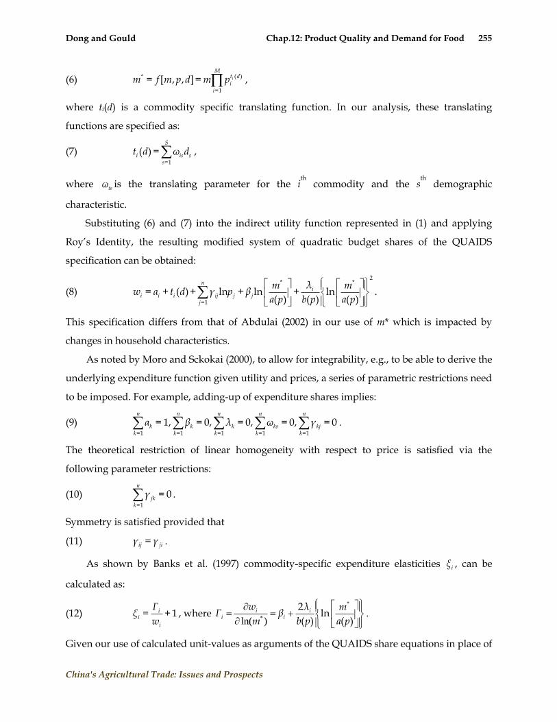
Dong and Gould Chap.12: Product Quality and Demand for Food 255
China's Agricultural Trade: Issues and Prospects
(6) ( )*
=1
= [ , , ]= i
Mt di
i
m f m p d m p ,
where ti(d) is a commodity specific translating function. In our analysis, these translating
functions are specified as:
(7) =1
( ) =S
i is ss
t d ω d ,
where isω is the translating parameter for the ith
commodity and the sth
demographic
characteristic.
Substituting (6) and (7) into the indirect utility function represented in (1) and applying
Roy‘s Identity, the resulting modified system of quadratic budget shares of the QUAIDS
specification can be obtained:
(8)
2* *
=1
= + ( )+ ln + ln + ln( ) ( ) ( )
ni
i i i ij j jj
λm mw α t d γ p β
a p b p a p.
This specification differs from that of Abdulai (2002) in our use of m* which is impacted by
changes in household characteristics.
As noted by Moro and Sckokai (2000), to allow for integrability, e.g., to be able to derive the
underlying expenditure function given utility and prices, a series of parametric restrictions need
to be imposed. For example, adding-up of expenditure shares implies:
(9) =1 =1 =1 =1 =1
= 1, = 0, = 0, = 0, = 0n n n n n
k k k ks kjk k k k k
α β λ ω γ .
The theoretical restriction of linear homogeneity with respect to price is satisfied via the
following parameter restrictions:
(10) =1
= 0n
jkk
γ .
Symmetry is satisfied provided that
(11) =ij jiγ γ .
As shown by Banks et al. (1997) commodity-specific expenditure elasticities iξ , can be
calculated as:
(12) = + 1ii
i
Γξ
w, where
*ln( )
i ii i
w λ mΓ β
m b p a p
*2ln
( ) ( ).
Given our use of calculated unit-values as arguments of the QUAIDS share equations in place of
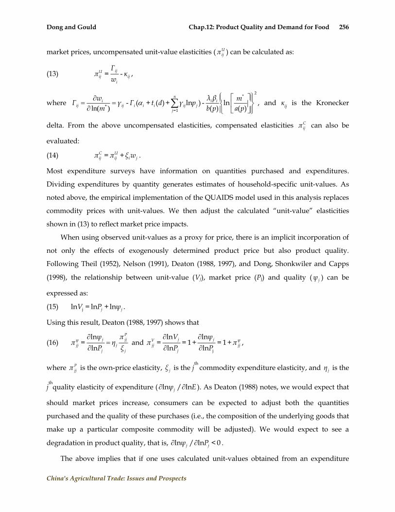
Dong and Gould Chap.12: Product Quality and Demand for Food 256
China's Agricultural Trade: Issues and Prospects
market prices, uncompensated unit-value elasticities ( Uijπ ) can be calculated as:
(13) = -ijU
ij ij
i
Γπ κ
w,
where *ln( )
n
i iiij ij i i i ij j
j
λ βw mΓ γ Γ t d γ p
m b p a p
2*
=1
- ( + ( )+ ln ) - ln( ) ( )
, and κij is the Kronecker
delta. From the above uncompensated elasticities, compensated elasticities Cijπ can also be
evaluated:
(14) C Uij ij i jπ π ξ w= + .
Most expenditure surveys have information on quantities purchased and expenditures.
Dividing expenditures by quantity generates estimates of household-specific unit-values. As
noted above, the empirical implementation of the QUAIDS model used in this analysis replaces
commodity prices with unit-values. We then adjust the calculated ―unit-value‖ elasticities
shown in (13) to reflect market price impacts.
When using observed unit-values as a proxy for price, there is an implicit incorporation of
not only the effects of exogenously determined product price but also product quality.
Following Theil (1952), Nelson (1991), Deaton (1988, 1997), and Dong, Shonkwiler and Capps
(1998), the relationship between unit-value (Vj), market price (Pj) and quality ( jψ ) can be
expressed as:
(15) jln = ln +lnj jV P ψ .
Using this result, Deaton (1988, 1997) shows that
(16)
Pj jjψ
jj j
j j
ψ ππ η
P ξ
ln=
ln and
j j ψVjj jj
j
V ψπ π
P Pj
ln ln= = 1+ = 1+
ln ln,
where Pjjπ is the own-price elasticity, jξ is the j
th commodity expenditure elasticity, and jη is the
jth
quality elasticity of expenditure ( ln / lnjψ E ). As Deaton (1988) notes, we would expect that
should market prices increase, consumers can be expected to adjust both the quantities
purchased and the quality of these purchases (i.e., the composition of the underlying goods that
make up a particular composite commodity will be adjusted). We would expect to see a
degradation in product quality, that is, ln / ln < 0j jψ P .
The above implies that if one uses calculated unit-values obtained from an expenditure

Dong and Gould Chap.12: Product Quality and Demand for Food 257
China's Agricultural Trade: Issues and Prospects
survey in the estimation of commodity demand elasticities and interprets them as such, these
demand elasticities incorporate both exogenous price and quality effects. Under the most usual
conditions, such elasticities tend to overstate the price elasticity in absolute magnitude if the
product of the price and quality elasticities is smaller than the expenditure elasticity. The above
relationships provide the framework for adjusting these ―demand‖ elasticities to control for
such quality effects.
Following Deaton (1997), from (16) the relationship between the own unit-value elasticity
ln( )=
ln( )
jUjj
j
d Qπ
d V and own-price elasticity
ln( )=
ln( )
jPjj
j
d Qπ
d P is:
(17) = =1+ / 1 - /
P Ujj jjU P
jj jjP Uj jj j j jj j
π ππ π
η π ξ η π ξ.
Dong, Shonkwiler and Capps (1998) and Dong and Gould (2000) incorporate the above into
a model originally formulated by Wales and Woodland (1980) to account for selectivity bias in
estimating a conditional commodity expenditure equation for a composite good while at the
same time endogenizing unit-value. Under their two-equation model, a unit-value regression
equation is formulated along with conditional expenditure functions where expenditure and
unit-value equation error terms are assumed to be normally distributed and correlated.
Parameters of the expenditure and price equations are estimated within a single likelihood
function encompassing all observations.
Deaton (1997) provides a general framework for incorporating product quality within an
empirical demand system. His methodology involves augmenting a system of utility-based
share equations with an associated set of unit-value equations. In his original specification, both
sets of dependent variables (i.e., expenditure shares and commodity unit-values) are dependent
on unobserved prices. Given the size of our empirical model and the complexity of the
functional form used, instead of using his method for solving for unobserved prices, we use
observed unit-values in the share equations and a set of market level variables in the unit-value
equations as instrumental variables for unobserved market prices. We then use the relationships
shown in (18) to transform the estimated unit-value elasticities ( Uijπ ) to price elasticities ( P
ijπ ).
We augment the QUAIDS share equations shown in (8) with the following unit value
equations:

Dong and Gould Chap.12: Product Quality and Demand for Food 258
China's Agricultural Trade: Issues and Prospects
(18) jln = +R D
*0j rj r dj d j
r=1 d=1
V τ τ R + τ D +υ ,
where the τ * ‘s and τ ‘s are coefficients to be estimated and Rr is the rth
regional dummy variable
used to capture the exogenous market price effects on observed unit-values.1 The vector of
variables represented by Dd corresponds to the set of demographic characteristics (including the
logarithm of total FAH expenditures) used as instruments for the unobserved product quality.
The share equations represented by (8) and the unit-value equations represented by (18)
represent our complete simultaneous system. It should be noted that only the expenditure share
equations have endogenous variables as arguments (i.e., lnVj). As noted by Greene (2003)
expressing all equations in a reduced form results in a likelihood function that is the same as the
seemingly unrelated regression equation where we assume all error terms to be related via a
multivariate normal distribution. A Full-Information Maximum Likelihood estimator is used to
obtain parameter values.
Chinese Urban Household Food Expenditure Data
The data used in this study are the same as used by Gould and Villarreal (2006) that are
obtained from an annual household expenditure survey conducted by the State Statistical
Bureau (SSB). These data encompass household expenditures for urban households in the
provinces of Jiangsu, Shandong, Guangdong, Heilongjiang and Henan for the year 2001. We use
an urban sample to avoid issues associated with the consumption of home produced foods. The
first three provinces are located on the China Sea. Jiangsu and Quangdong are the most
prosperous provinces given their location close to Shanghai and Hong Kong, respectively
(Table 1). The latter two provinces are the poorest of the five. Both are located in the interior
with Heilongjiang being the most north and Henan located west of Shandong. In addition to
food purchase quantity and value, household and member demographic characteristics are also
included in this data set. A total of 3,650 households were used to estimate the parameters of
our food system (Table 2).
1 This implies that when estimating the share equations we use predicted unit values instead of observed unit values or unobserved market prices.

Dong and Gould Chap.12: Product Quality and Demand for Food 259
China's Agricultural Trade: Issues and Prospects
Table 1: Allocation of Food Expenditures across Food Commodity Group, Expenditure Decile and Region
Entire Sample
Lowest Decile
Highest Decile
Jiangsu Shandong Guangdong Henan Heilongjiang
Beef 8.6 7.1 11.4 8.4 8.0 11.4 7.6 9.4 Pork 10.4 11.7 9.5 10.9 9.5 10.2 12.7 11.1
Poultry 5.7 3.9 14.5 6.3 6.0 9.7 5.7 3.0
Seafood/Fish 7.9 4.5 11.3 11.1 7.3 14.1 3.0 5.8
Vegetables 11.3 13.8 4.5 10.8 9.8 11.4 12.6 13.6
Rice 5.0 6.9 8.8 6.3 2.0 4.9 4.4 7.1
Other Grain 7.6 13.4 5.9 3.4 9.2 4.2 14.1 9.6
Fruit 7.8 7.8 4.2 5.7 7.9 7.9 7.6 10.6
Dairy 5.0 3.2 5.9 5.3 6.9 4.6 4.1 4.8
Eggs 4.1 6.6 1.9 3.4 5.4 1.7 6.2 4.9
Fats/Oils 3.4 5.1 2.5 3.1 2.7 2.4 5.4 4.3
Other Food 15.4 16.1 15.8 16.3 17.7 13.6 16.6 15.8
Total Food Expend. (Yuan)
6,356 2,043 16,476 6,426 5,071 13,083 4,128 4,435
Food-at-Home (FAH) Expend.
(Yuan)
5,135 1,790 11,604 5,335 4,242 9,234 3,660 3,983
Household Income(Yuan)
23,661 10,931 56,990 22,961 20,588 47,446 15,884 16,612
Income as % of All Urban Chinese
116.1 53.6 279.7 112.7 101.0 232.8 67.1 70.2
Food Expend. As % of Income
26.8 18.7 28.9 28.0 24.6 27.6 26.0 26.7
FAH* as % of Income
21.7 17.4 19.7 23.2 20.6 19.5 23.0 24.0
Sample Size 3650 365 365 800 650 600 600 1000 *Note: During June 2001, 1 $US = 8.28 Yuan. In 2001, the average urban household income across all Chinese provinces was 20,378 yuan (National Bureau of Statistics, 2003). The decile categories in the above table are defined relative to total food expenditures.
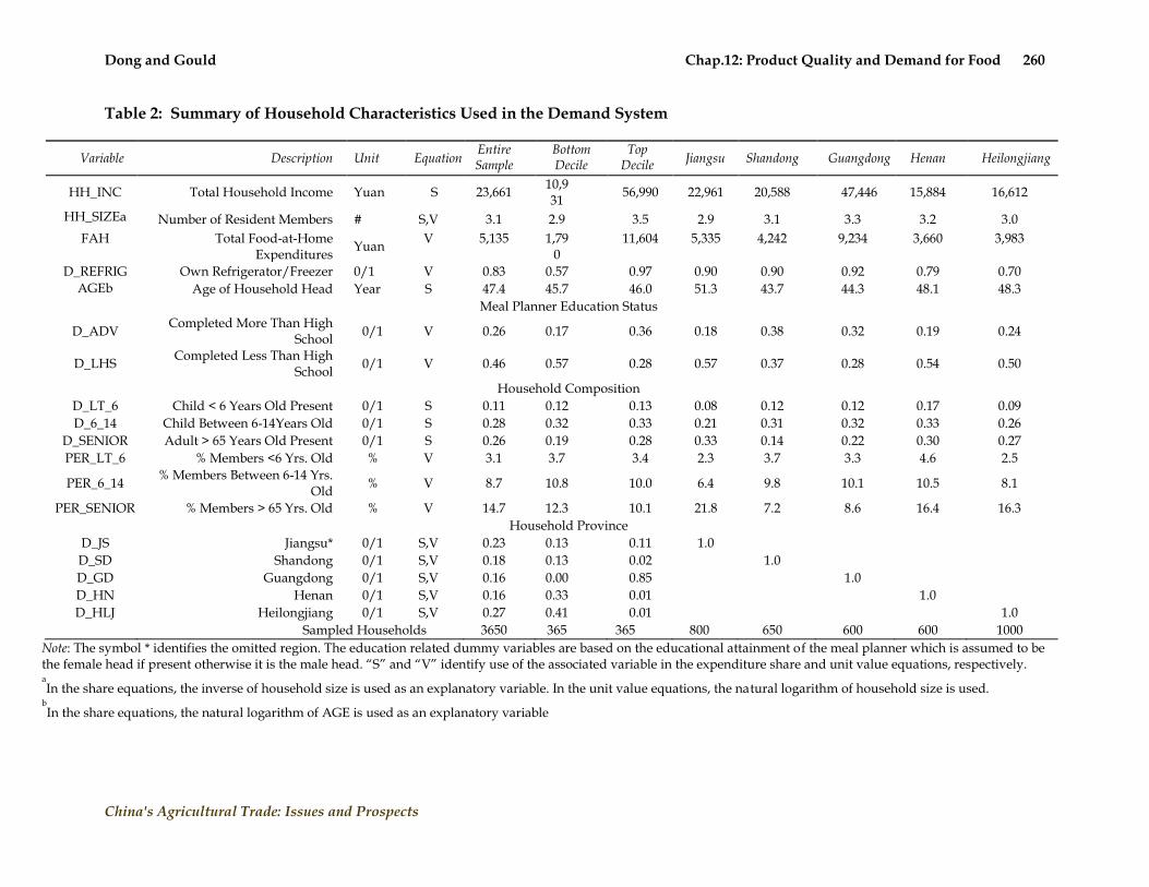
Dong and Gould Chap.12: Product Quality and Demand for Food 260
China's Agricultural Trade: Issues and Prospects
Table 2: Summary of Household Characteristics Used in the Demand System
Variable Description Unit Equation Entire Sample
Bottom Decile
Top Decile
Jiangsu Shandong Guangdong Henan Heilongjiang
HH_INC Total Household Income Yuan S 23,661 10,931
56,990 22,961 20,588 47,446 15,884 16,612
HH_SIZEa Number of Resident Members # S,V 3.1 2.9 3.5 2.9 3.1 3.3 3.2 3.0
FAH Total Food-at-Home Expenditures
Yuan V 5,135 1,79
0 11,604 5,335 4,242 9,234 3,660 3,983
D_REFRIG Own Refrigerator/Freezer 0/1 V 0.83 0.57 0.97 0.90 0.90 0.92 0.79 0.70
AGEb Age of Household Head Year S 47.4 45.7 46.0 51.3 43.7 44.3 48.1 48.3
Meal Planner Education Status
D_ADV Completed More Than High
School 0/1 V 0.26 0.17 0.36 0.18 0.38 0.32 0.19 0.24
D_LHS Completed Less Than High
School 0/1 V 0.46 0.57 0.28 0.57 0.37 0.28 0.54 0.50
Household Composition
D_LT_6 Child < 6 Years Old Present 0/1 S 0.11 0.12 0.13 0.08 0.12 0.12 0.17 0.09
D_6_14 Child Between 6-14Years Old 0/1 S 0.28 0.32 0.33 0.21 0.31 0.32 0.33 0.26
D_SENIOR Adult > 65 Years Old Present 0/1 S 0.26 0.19 0.28 0.33 0.14 0.22 0.30 0.27
PER_LT_6 % Members <6 Yrs. Old % V 3.1 3.7 3.4 2.3 3.7 3.3 4.6 2.5
PER_6_14 % Members Between 6-14 Yrs.
Old % V 8.7 10.8 10.0 6.4 9.8 10.1 10.5 8.1
PER_SENIOR % Members > 65 Yrs. Old % V 14.7 12.3 10.1 21.8 7.2 8.6 16.4 16.3
Household Province
D_JS Jiangsu* 0/1 S,V 0.23 0.13 0.11 1.0
D_SD Shandong 0/1 S,V 0.18 0.13 0.02 1.0
D_GD Guangdong 0/1 S,V 0.16 0.00 0.85 1.0
D_HN Henan 0/1 S,V 0.16 0.33 0.01 1.0
D_HLJ Heilongjiang 0/1 S,V 0.27 0.41 0.01 1.0
Sampled Households 3650 365 365 800 650 600 600 1000
Note: The symbol * identifies the omitted region. The education related dummy variables are based on the educational attainment of the meal planner which is assumed to be the female head if present otherwise it is the male head. ―S‖ and ―V‖ identify use of the associated variable in the expenditure share and unit value equations, respectively. aIn the share equations, the inverse of household size is used as an explanatory variable. In the unit value equations, the natural logarithm of household size is used.
bIn the share equations, the natural logarithm of AGE is used as an explanatory variable

Dong and Gould Chap.12: Product Quality and Demand for Food 261
China's Agricultural Trade: Issues and Prospects
In the expenditure survey, households maintain detailed daily expenditure diaries related
to the purchase of food and nonfood items over the entire survey year. The daily diaries are
then summarized by county statistical offices and aggregate results for each expenditure item
and household reported to the SSB. The annual nature of these diaries is in contrast to other
developing country surveys that typically encompass 1-2 weeks of purchases (Dong et al., 2004;
Sabates et al., 2001). The brevity of the data collection period in these other setting usually
results in the censoring of food expenditures. Such censoring represents a significant
econometric problem when estimating disaggregated food demand systems (Dong et al., 2004;
Perali and Chavas, 2000; Yen et al., 2003). Given the annual nature of the expenditure diaries
used here, even with the development of our 12 food demand system, commodity censoring
was not a problem.
For our analysis we adopt commodity group definitions similar to the categories used by
Gao et al. (1996), in their analysis of Chinese household food purchase behavior. These food
categories include beef/mutton (BF), pork (PK), poultry (PLT), fish/seafood (SFD), vegetables
(VEG), fruits (FRT), rice (RIC), other grain products (OGR), dairy products (DA), eggs (EGG),
food fats and oils (FAT), and other foods for at-home consumption (OTH).2
Table 2 provides an overview of food purchase patterns of our sampled households. Mean
annual household income ranges from 15,884 yuan/household in Henan province to 47,446
yuan in Guongdong. In spite of this wide range there is little variation in the mean share of
household income allocated to food. The minimum mean food share is 24.6% for households in
Shandong province. This compares to 28.0% for households in Jiangsu province. In contrast,
there are some significant differences in the allocation of average household food budgets
across specific food categories. For example, Guongdong, the more affluent province, relies the
least on grain-based commodities (7.0% of total food expenditures) while households in Henan
rely the most (17.0% of expenditures). For the 5 provinces included in this analysis, the sample
mean income is 16.1% greater than the mean household income across all urban Chinese
households. Again the relative value of this value varies across province, from slightly more
than 66% for our sample of households from Henan province to more than 230% for our sample
2 A detailed listing of the commodities contained in these categories can be obtained from the authors upon request. For those rare occasions were a household did not report purchasing a particular commodity category, the average unit-value for that commodity in that households particular city/county were used in the econometric model. FAFH is not included in the current analysis given the difficulty with defining the unit-value of FAFH purchases. For an example of a study that includes FAFH in a food demand system, see Perali and Chavas (2000).

Dong and Gould Chap.12: Product Quality and Demand for Food 262
China's Agricultural Trade: Issues and Prospects
of urban Guangdong households.
Besides data sorted by region of residence, we also present food purchase characteristics for
households contained in the highest and lowest total food expenditure deciles. Not
surprisingly, the most significant difference can be seen with respect to the importance of FAFH
as a food source. Slightly less than one-third of total food expenditures by households in the
highest expenditure decile, is spent on FAFH. This compares to only 7% for households in the
lowest expenditure decile. More than 35% of FAH expenditures is associated with beef, pork or
poultry for the highest decile households. This compares to less than 23% for households in the
lowest decile. The lowest decile households also spend relatively more on vegetables compared
to high decile households.
We account for household heterogeneity in the estimated expenditure share equations by
including a set of demographic characteristics in the translating functions, ti(p). Table 2
provides an overview of these characteristics along with the household characteristics used in
the unit-value equations. Besides the wide range in household income across region noted in
Table 1, there is a parallel pattern obtained with respect to the percent of households owning
refrigerators and/or freezer appliances (D_REFRIG) and meal planner education (D_ADV,
D_LHS).
Approximately 17% of the sampled households indicated they did not own a refrigerator or
freezer. The ownership of refrigerated storage has previously been shown to be important
determinants of food choice in other developing country settings (Gould and Villarreal, 2002).
The presence of refrigerated storage can impact not only the purchase choice of perishable
versus nonperishable commodities but also their frequency of purchase (Blundell and Meghir,
1987). Given our survey encompasses an entire year of purchase history; infrequency-of-
purchase is not felt to be an important issue. Only 70% of sampled households in Heilongjiang
province possessed refrigerated storage. This compares to more than 92% of the sampled
households in Guangdong province. Less than 60% of households had refrigerated storage
facilities in the lowest expenditure decile compared to more than 97% in the highest decile.
Previous analyses have also shown that educational attainment of the main meal planner
has an impact on food choice and nutritional quality of the resulting diets (Sabates et al., 2001).
That is, we hypothesize a positive relationship between meal planner education and diet
quality. Overall, approximately 46% of the household meal planners did not have a high school
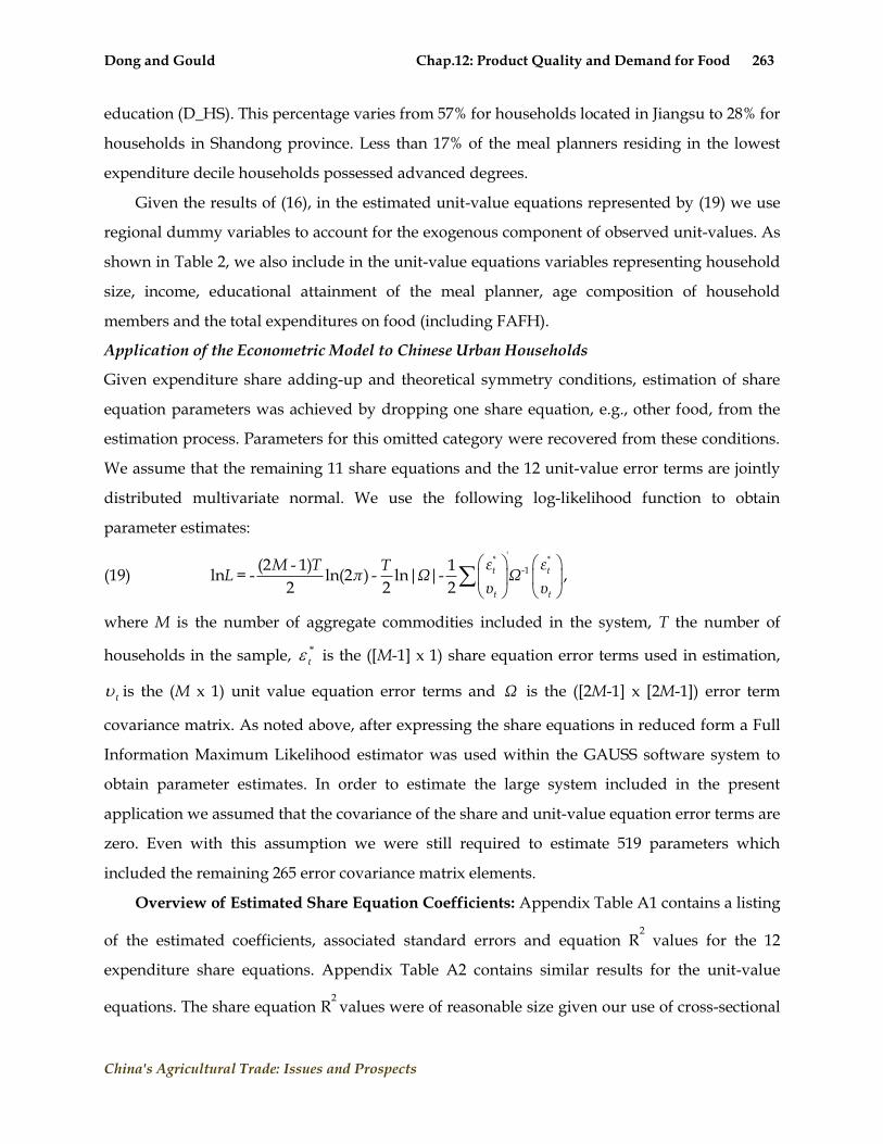
Dong and Gould Chap.12: Product Quality and Demand for Food 263
China's Agricultural Trade: Issues and Prospects
education (D_HS). This percentage varies from 57% for households located in Jiangsu to 28% for
households in Shandong province. Less than 17% of the meal planners residing in the lowest
expenditure decile households possessed advanced degrees.
Given the results of (16), in the estimated unit-value equations represented by (19) we use
regional dummy variables to account for the exogenous component of observed unit-values. As
shown in Table 2, we also include in the unit-value equations variables representing household
size, income, educational attainment of the meal planner, age composition of household
members and the total expenditures on food (including FAFH).
Application of the Econometric Model to Chinese Urban Households
Given expenditure share adding-up and theoretical symmetry conditions, estimation of share
equation parameters was achieved by dropping one share equation, e.g., other food, from the
estimation process. Parameters for this omitted category were recovered from these conditions.
We assume that the remaining 11 share equations and the 12 unit-value error terms are jointly
distributed multivariate normal. We use the following log-likelihood function to obtain
parameter estimates:
(19)
'
-1(2 - 1) 1ln = - ln(2 ) - ln| |-
2 2 2
* *t t
t t
ε εM T TL π Ω Ω
υ υ,
where M is the number of aggregate commodities included in the system, T the number of
households in the sample, *
t is the ([M-1] x 1) share equation error terms used in estimation,
t is the (M x 1) unit value equation error terms and Ω is the ([2M-1] x [2M-1]) error term
covariance matrix. As noted above, after expressing the share equations in reduced form a Full
Information Maximum Likelihood estimator was used within the GAUSS software system to
obtain parameter estimates. In order to estimate the large system included in the present
application we assumed that the covariance of the share and unit-value equation error terms are
zero. Even with this assumption we were still required to estimate 519 parameters which
included the remaining 265 error covariance matrix elements.
Overview of Estimated Share Equation Coefficients: Appendix Table A1 contains a listing
of the estimated coefficients, associated standard errors and equation R2 values for the 12
expenditure share equations. Appendix Table A2 contains similar results for the unit-value
equations. The share equation R2
values were of reasonable size given our use of cross-sectional

Dong and Gould Chap.12: Product Quality and Demand for Food 264
China's Agricultural Trade: Issues and Prospects
data ranging from 0.029 for pork to 0.436 for other grains. It was not surprising that the R2
values for the unit-value equations tended to be larger than the share equation values given the
use of lnV as the dependent variable. The range in unit value R2 values was from 0.082 for dairy
products to 0.688 for the fruit commodity.
As shown in Appendix Table A1, there are 11 demographic-related coefficients in each
share equation resulting in 132 share equation demographic related parameters. Approximately
two-thirds of these coefficients were statistically significant at the 0.01 level. There appears to be
significant regional differences in the structure of food demand as 40 of the 48 provincial
dummy variable coefficients were statistically significant. Compared to the impact of region on
food demand structure we found less of an impact of household age composition. Less than a
third of the age related dummy variable coefficients were found to be statistically significant.
Not surprisingly, for dairy products we see that having children in the household positively
impacts the share of total expenditures allocated to dairy products. Having adults over the age
of 65 in the household only impacted expenditures on fruits (-) and rice (+).
We included household head age (AGE) as an explanatory variable in the share equations
to capture some of the age-related cohort effects in food choice. From Appendix Table A1, we
see that head age is negatively related to the share of total food expenditures allocated to beef,
poultry, fruits and dairy products. We also find some evidence that household income impacts
food choice. The estimated coefficients associated with household income in the share equation
were statistically significant except in for the poultry equations. The level of food expenditure
shares associated with beef, fruit, and dairy products were positively related to household
income.
We hypothesized that refrigerator ownership would have a positive impact on the share
of relative expenditures spend on commodities considered to be perishable. Except for the other
foods category, the commodities where a positive impact of refrigerator ownership was for
commodity groups that could be considered being composed of perishable foods (e.g., beef,
seafood, fruit, and dairy products).
From Appendix Table A1 we see that a majority of price related coefficients are
significantly different from zero (i.e., 65 out of 78). The beef and poultry commodities had the
least number of statistically significant price coefficients. The price coefficients associated with
the dairy products (10 out of 12) and other food categories (12 out of 12) had the largest number

Dong and Gould Chap.12: Product Quality and Demand for Food 265
China's Agricultural Trade: Issues and Prospects
of statistically significant coefficients.
Overview of the Estimated Coefficients in the Unit Value Equations: Appendix Table
A2 contains the estimated coefficients associated with the unit-value equations. As noted above
we use the regional dummy variables to provide an estimate of exogenous market prices (i.e.,
lnPj). There are significant regional differences in commodity prices as reflected in 40 of the 48
estimated regional dummy coefficients being statistically significant from the base region,
Shandong. Market prices in Guangdong and Jiangsu provinces are tend to be higher versus
those in Henan and Heilongjiang provinces. This result is not surprisingly given the relative
income levels in these provinces (Table 1).
We initially hypothesize a negative relationship between household size and observed unit
values reflecting a household‘s ability to obtain economies of scale when purchasing larger
quantities. Dong and Gould (2000) found such an effect in their analysis of purchases of pork
and poultry purchases. We do not find evidence of this in the present application with
significant negative values obtained in the fats and oils and other food commodity groupings.
There appears to be some relationship between education level and unit-value. This
suggests that more educated households exhibited an increased demand for quality, ceteris
paribus. Household composition appears to matter in terms of the demand for food quality.
Unit-values for 5 of the 12 commodities are impacted by the percentage of household members
that are older than 65 years. The beef commodity shows a positive unit-value relationship
compared to negative values obtained in the vegetable, fruit, other grain and dairy product unit
value equations. All of the unit value coefficients associated with the PER_LT_6 and PER_6_14
variables were positive, indicating increased demand for quality. Again, this may be reflecting a
cohort effect where younger households being accustomed to purchasing better quality food.
Evaluation of the Structure of Food Demand: From (12) expenditure elasticities ( j ) are
calculated using the mean values of the exogenous variables and displayed in Table 3. Banks et
al. (1997) note that given the expression for the expenditure elasticities shown in (12) a positive
iβ coefficient in combination with a negative iλ value implies for relatively low expenditure
levels, the ith
commodity could be considered a luxury and a necessity for relatively high
expenditure levels. Only the pork commodity exhibits this structure. It was surprising that
dairy products did not fall into this category given the historically low levels of dairy product
expenditures in the past and rapid increases in such expenditures recently.

Dong and Gould Chap.12: Product Quality and Demand for Food 266
China's Agricultural Trade: Issues and Prospects
Table 3: Uncompensated Unit-Value and Expenditure Elasticities
Quantity Change
BF PK PLT SFD VEG FRT RI OG DA EG FAT OTH
Pri
ce C
han
ge
BF -0.968 0.095 -0.008 0.022 -0.012 -0.015 0.014 -0.022 -0.042 -0.013 -0.026 -0.167
PK 0.071 -0.579* 0.018 -0.110 0.053 -0.094 -0.022 -0.026 -0.126 0.041 0.013 -0.515
PLT -0.011 0.045 -0.876* 0.021 0.020 -0.040 -0.160 0.011 0.045 0.063 -0.037 -0.211
SFD 0.027 -0.140 0.017 -0.608* -0.075 0.044 -0.122 0.041 -0.022 -0.073 -0.009 -0.057
VEG -0.005 0.056 0.013 -0.052 -0.678* -0.046 0.010 -0.124 -0.040 -0.063 0.023 -0.049
FRT 0.001 -0.104 -0.017 0.048 -0.063 -0.704* -0.126 0.033 0.066 -0.094 -0.040 0.277
RI 0.021 -0.058 -0.183 -0.193 0.025 -0.185 -0.603* 0.126 -0.116 0.285 0.153 -0.241
OG 0.001 0.000 0.026 0.046 -0.180 0.029 0.074 -1.019 0.096 -0.061 -0.087 0.436
DA -0.067 -0.235 0.054 -0.040 -0.101 0.070 -0.114 0.102 -0.405* -0.065 -0.049 -0.339
EG -0.020 0.114 0.090 -0.138 -0.171 -0.180 0.338 -0.117 -0.070 -0.737* 0.002 -0.052
FAT -0.073 0.037 -0.066 -0.023 0.069 -0.102 0.225 -0.209 -0.081 -0.001 -0.713* -0.275
OTH -0.036 -0.216 -0.043 -0.037 -0.058 0.043 -0.085 0.093 -0.064 -0.025 -0.028 -0.510*
Expenditure Elasticity
1.142 1.277 1.130 0.977 0.954 0.722 0.968 0.639 1.191 0.941 1.215 0.966
Note: The above elasticities were evaluated at the mean values of the exogenous variables. For the unit value elasticities, shaded values identify those that are statistically different from 0 with a 0.01 Pr(Type I Error). For the expenditure elasticities a shaded value identifies elasticities statistically different from 1.0. For own unit value elasticities, a ―*‖ indicates a value statistically different from -1.0 at the 0.01 significance level

Dong and Gould Chap.12: Product Quality and Demand for Food 267
China's Agricultural Trade: Issues and Prospects
When evaluated at these mean values of the exogenous variables we find that beef, pork, dairy
products and fats and oils have expenditure elasticities significantly greater than 1.0. Given the
relative increase in per capita fruit consumption in recent history, it is surprising that the
estimated fruit expenditure elasticity is significantly less than 1.0.
Table 3 also contains a summary of the estimated uncompensated (Marshallian) unit-value
elasticities, Uijπ , via (14). All own unit-value elasticities were found to be significantly less than
zero and all except for the other grains commodity were inelastic. Surprisingly, dairy products
exhibited the most own unit-value inelastic structure. In terms of the cross price effects we
found a mixture of gross complements and substitutes. Of the 132 cross unit-value elasticities,
77 were found to be statistically different from 0. The large number of significant relationships
reinforces the need for us to disaggregate our analysis of food purchases versus the more ad hoc
single equation approaches. Of the statistically significant cross unit-value elasticities all exhibit
inelastic relationships. The relationship between demands for other food commodities due to a
change in unit-value of the other grains commodity shows the largest substitution relationship
with a cross-price elasticity of 0.436. The next largest substitute relationship was between the
demand for rice in reaction to changes in the egg unit value. An example of a complementary
relationship can be seen for the impact on other food demand resulting from the pork unit
value, -0.515.
Differentiation of Unit Value and Price Elasticities: Deaton (1988; 1997) provides the
theoretical framework for differentiating the effects on food choice of changes in endogenously
determined unit values versus exogenous market prices. As noted above, Table 3 contains
elasticity measures that incorporate quality effects. To isolate the quality effects of price
changes, Table 4 provides a summary of alternative elasticity measures used to correctly
evaluate the own-price impacts on commodity demand.
Similar to the interpretations of Prais and Houthaaker (1955), Cramer (1973) and Deaton
(1997) we interpret the elasticity of unit value to a change in total expenditures (FAH), as a
measure of the quality elasticity, e.g.
j j
j
ψ Vη = =
E FAH
ln ln
ln ln. These elasticity values are displayed
in the first column of Table 4. They are relatively small but much larger than those obtained by
Myrland et al. (2003) in their analysis of the demand for salmon (0.002) which was based on a
similar methodology as used here but applied to a single commodity.

Dong and Gould Chap.12: Product Quality and Demand for Food 268
China's Agricultural Trade: Issues and Prospects
Table 4: Comparison of Various Elasticity Measures
Commodity
Quality
( j )
[1]
Unit Value
(U
jj )
[2]
Own Price (P
jj ) Unit-Value Own Price (V
jj ) Quality Own Price ( jj )
Base [3]
2X [4]
3X [5]
Base [6]
2X [7]
3X [8]
Base [9]
2X [10]
3X [11]
BF 0.093 (0.021)
-0.968 (0.021)
-0.898 (0.025)
-0.837 -0.784 0.927 (0.016)
0.864 0.810 -0.073 (0.016)
-0.136 -0.190
PK 0.059 (0.005)
-0.579 (0.060)
-0.564 (0.057)
-0.550 -0.536 0.974 (0.004)
0.949 0.926 -0.026 (0.004)
-0.051 -0.074
PLT 0.139 (0.013)
-0.880 (0.046)
-0.794 (0.039)
-0.723 -0.664 0.902 (0.010)
0.822 0.754 -0.098 (0.010)
-0.178 -0.246
SFD 0.250 (0.015)
-0.608 (0.028)
-0.526 (0.020)
-0.464 -0.414 0.865 (0.013)
0.763 0.682 -0.135 (0.013)
-0.237 -0.318
VEG 0.287 (0.013)
-0.678 (0.022)
-0.563 (0.016)
-0.482 -0.421 0.831 (0.008)
0.710 0.621 -0.169 (0.008)
-0.290 -0.379
FR 0.254 (0.015)
-0.704 (0.033)
-0.564 (0.024)
-0.471 -0.404 0.802 (0.015)
0.669 0.574 -0.198 (0.015)
-0.331 -0.426
RIC 0.071 (0.007)
-0.603 (0.086)
-0.577 (0.079)
-0.554 -0.532 0.957 (0.008)
0.918 0.882 -0.043 (0.008)
-0.082 -0.118
OGR 0.140 (0.016)
-1.019 (0.035)
-0.833 (0.029)
-0.704 -0.610 0.817 (0.020)
0.691 0.598 -0.183 (0.020)
-0.309 -0.402
DA 0.180 (0.017)
-0.405 (0.055)
-0.382 (0.049)
-0.361 -0.342 0.942 (0.009)
0.891 0.845 -0.058 (0.009)
-0.109 -0.155
EGG 0.032 (0.006)
-0.737 (0.072)
-0.719 (0.068)
-0.702 -0.685 0.975 (0.005)
0.952 0.930 -0.025 (0.005)
-0.048 -0.070
FAT 0.113 (0.011)
-0.713 (0.065)
-0.669 (0.057)
-0.630 -0.595 0.938 (0.009)
0.883 0.835 -0.062 (0.009)
-0.117 -0.165
OTH 0.311 (0.014)
-0.510 (0.038)
-0.438 (0.030)
-0.384 -0.342 0.859 (0.008)
0.753 0.670 -0.141 (0.008)
-0.247 -0.330
Note: The terms ―2X‖ and ―3X‖ refer to estimates based on values of the Quality Elasticity, ?j, being 2 and 3 times as large as the values displayed in column (1). Standard deviations are in parentheses. Standard deviations are not presented for the 2X and 3X simulations as they required an assumption concerning the associated standard deviation of the underlying coefficients.

Dong and Gould Chap.12: Product Quality and Demand for Food 269
China's Agricultural Trade: Issues and Prospects
Dong and Gould (2000) in their double-hurdle model of pork and poultry purchases by
Mexican households obtain similar values as those reported in Table 4, 0.060 and 0.10,
respectively. In the analysis of food demand in urban households in Pakistan (1984-85), Deaton
(1997) obtained a relatively large value for his aggregate meat category, 0.242 when compared
to the estimated values obtained for our beef, pork and poultry commodities.
The second column of Table 4 repeats the value of the own unit value elasticities previously
reported in Table 3. The next 3 columns use the results of (17) to summarize our estimates of the
own-price elasticities, Pjjπ under alternative expenditure elasticity scenarios. Similar the results
of Deaton (1997) the relatively small quality elasticities result in small differences in Ujjπ versus
Pjjπ values. The P
jjπ values shown under the Base column correspond to the values obtained
using the quality elasticities obtained from the estimated unit value equations. Only for the fruit
and other grains commodities do we see a major difference between the unit-value versus price
based elasticity measures. Next to the Base model we present our estimates of the own price
elasticity if the quality elasticity had been double (2X) or triple (3X) the estimated value.
Given our estimates of Pjjπ we use (17) to generate estimates of the relationship between
observed unit-values and unobserved market prices, e.g.,
ln=
ln
jPjj
j
Vπ
P. These estimates are
provided in columns 6-8 of Table 4 based on the same quality elasticity values used in the
evaluation of the price elasticities. We would expect that 0< Vjjπ <1. The higher the number the
lower the role quality plays in determining observed unit-values. The range in values was from
0.975 for eggs to 0.817 and 0.802 for the other grains and fruit categories, respectively. The
relatively large value for eggs is not surprising given the egg commodity is composed of mostly
a single fundamental good, chicken eggs which is fairly standardized. In contrast, the other
grains category is composed of a number of different types of fundamental goods some with
very little valued added characteristics such as raw small grains versus others that embody
significant value added, e.g., breads and bakery items. The relatively high Vjjπ values for the
meat categories and for dairy products were surprising given the variety of product forms and
degree of processing associated with composite commodities. Similar to the analysis of Pjjπ we
also examine the sensitivity of Vjjπ to alternative quality elasticity.

Dong and Gould Chap.12: Product Quality and Demand for Food 270
China's Agricultural Trade: Issues and Prospects
Given the definition of unit-values and the relationship between observed unit-values,
product price and quality noted in (15), the quality own price elasticity
jψjj
j
ψπ =
P exhibits the
opposite pattern of the above unit-value own price elasticity. That is, the quality of the Other
Grain and Fruit commodities responded the most to changes in unit-values.
We verify the theoretical results of Deaton (1988; 1997) by finding that for all commodities,
a price increase, ceteris paribus, will result not only in a reduction in quantity purchased but
also a reduction in the quality of the composite commodity bundle. If the quality elasticity for
the Fruit commodity had been 0.508 versus the actual value of 0.254, the quality own-price
elasticity is projected to increase in absolute value from 0.198 to 0.331.
Summary
This research utilizes a generalization of the Quadratic Almost Ideal Demand System (QUAIDS)
to quantify the structure of food demand of urban households in 5 Chinese provinces. We
extend previous research via the estimation of a disaggregated demand system while at the
same time accounting for the endogenous decision as to product quality. By capturing the joint
nature of the quantity and quality decisions we are able to examine the impact of quality when
market prices change. As predicted, increases in market prices result in changes in purchase
patterns such that overall commodity quality is reduced.
The results presented in this chapter show that there are statistically significant
substitution effects between foods. The utilization of the QUAIDS specification was important
as a likelihood ratio test indicated that this specification added significant explanatory power to
the model versus the traditional AIDS specification. Using the QUAIDS specification we obtain
reasonable unit value and price elasticity estimates when compared to other analyses of food
demand by Chinese households.
Our method for examining the impacts of product quality results in a set of elasticity
measures that indicate that product quality is relatively inelastic with respect to changes in
market prices. The analysis presented here is based on demand characteristics for the sample as
a whole. A more detailed analysis should examine how the demand for quality varies across
households in different income deciles, expenditure deciles, region of residence, etc. We also
need to provide estimated cross-price elasticities using the estimated cross unit-value
elasticities. These values will enable us to answer the question as to whether the similarity of the

Dong and Gould Chap.12: Product Quality and Demand for Food 271
China's Agricultural Trade: Issues and Prospects
own price and own unit-value elasticities carries over to cross price effects.
An extension of the current model would be to examine the sensitivity of our results to
changes in the method by which we endogenize product quality. That is, in the estimated
QUAIDS share equations we use predicted simultaneously determined unit values instead of
unobserved commodity market prices as explanatory variables. This is in contrast to the
methodology proposed by Deaton (1997) whereby both the system of share equations and unit
value equations use the unobserved commodity market prices as explanatory variables. He
applies this methodology to a Linear Approximate AIDS-based system. Our use of the much
more nonlinear QUAIDS model greatly complicates the implementation of Deaton‘s (1997)
framework. In the future, we will undertake the task of incorporating his methodology within
the QUAIDS structure.
There is no doubt that China is becoming more of an important market for U.S. food
manufacturers and marketers. As domestic income levels improve the demand for specific
foods will change not only in terms of the amount demanded but also in terms of product
quality. U.S. firms desiring to access the Chinese food market need to recognize this demand for
product quality. The current analysis indicates that there is a quantity versus quality tradeoff
but to this point such a relationship varies across commodity but in general is relatively minor.
Future research, using more recent food expenditure data, will be used to evaluate whether
product quality adjusts to commodity price changes becomes more important.
References Abdulai, A. ―Household Demand for Food in Switzerland: A Quadratic Almost Ideal Demand
System,‖ Swiss Journal of Economics and Statistics 138(2002): 1-18. Atkinson, A.B., J. Gomulka, and N.H. Stern. ―Spending on Alcohol: Evidence from the Family
Expenditure Sur vey 1970-1983,‖ Economic Journal 100(1990): 808-827. Banks, J., R. Blundell, and A. Lewbel. ―Tax Reform and Welfare Measurement: Do We Need
Demand System Estimation,‖ Economic Journal 106(1996): 1227-1241. Banks, J., R. Blundell, and A. Lewbel. ―Quadratic Engel Curves and Consumer Demand,‖
Review of Economics and Statistics 79(1997): 527-539.
Barten, A.P. 1964. ―Family Composition, Prices and Expenditure Patterns.‖ In the 16th
Symposium of the Colston Society, P.G. Hart, G. Mills, and J.K. Whittaker (eds.). London: Econometric Analysis for National Economic Planning.
Blundell, R.W., and C. Meghir. ―Bivariate Alternatives to the Tobit Model,‖ Journal of Econometrics 34(1987): 179-200.
Blundell, R. P. Pashardes, and G. Weber. ―What Do We Learn about Consumer Demand from Micro Data?‖ American Economic Review 83(1993): 570-597.

Dong and Gould Chap.12: Product Quality and Demand for Food 272
China's Agricultural Trade: Issues and Prospects
Cox, T.L.,and M.K. Wohlgenant. ―Prices and Quality Effects in Cross-Sectional Demand Analysis,‖ American Journal Agricultural Economics 68(1986): 908–919.
Cramer, J.S. ―Interaction of Income and Price in Consumer Demand,” International Economic Review 14(1973):351-363.
Deaton, A. ―Quality, Quantity, and Spatial Variation of Price,‖ American Economic Review 78(1988):418-430.
Deaton, A. The Analysis of Household Surveys: A Microeconometric Approach to Development Policy. Baltimore: Johns Hopkins University Press (1997).
Deaton, A. and J. Muellbauer. ―An Almost Ideal Demand System,‖ American Economic Review 70(1980): 312-336.
Dong, D. and B.W. Gould. ―Quality versus Quantity in Mexican Household Poultry and Pork Purchases,‖ Agribusiness: An International Journal 16(2000): 33-356.
Dong, D., B.W. Gould, and H.M. Kaiser. ―Food Demand in Mexico: An Application of the Amemiya-Tobin Approach to the Estimation of a Censored Food System,‖ American Journal of Agricultural Economics 86(2004): 1094-1107.
Dong, D., J.S. Shonkwhiler, and O. Capps. ―Estimation of Demand Functions Using Cross-Sectional Household Data: The Problem Revisited,‖ American Journal Agricultural Economics 80(1998): 466–473.
Gale, F. ―China‘s Growing Affluence: How Food Markets are Responding,‖ Amber Waves. Washington DC: Economic Research Service, USDA (2003).
Gao, X.M, E.J.Wailes, and G.L. Cramer. ―A Two-Stage Rural Household Demand Analysis: Microdata Evidence from Jiangsu Province, China,‖ American Journal of Agricultural Economics 78(1996): 604-13.
Gould, B.W. ―Factors Affecting U.S. Demand for Reduced-Fat Fluid Milk,‖ Journal of Agricultural and Resource Economics 21(1996): 68–81.
Gould, B.W., T.L. Cox, and F. Perali. ―Demand for Food Fats and Oils: The Role of Demographic Variables and Government Donations,‖ American Journal of Agricultural Economics 73(1991): 212-221.
Gould, B.W., and H.J. Villarreal. ―Adult Equivalence Scales and Food Expenditures: An Application to Mexican Beef and Pork Purchases,‖ Applied Economics 34(2002): 1075-88.
Gould, B.W., and H.J. Villarreal. ―An Assessment of the Current Structure of Food Demand in Urban China,‖ Agricultural Economics 34(2006): 1-16.
Greene, W. Econometric Analysis. New York: Prentice Hall (2003). Guo, X., T.A. Mroz, B.M. Popkin, and F. Zhai. ―Structural Change in the Impact of Income on
Food Consumption in China, 1989-1993,‖ Economic Development and Cultural Change 48(2000): 737-60.
Hausman, J.A., W.K. Newey, and J.L.Powell. ―Nonlinear Errors in Variables: Estimation of Some Engel Curves,‖ Journal of Econometrics 65(1995): 205-233.
Heien, D. and G. Pompelli. ―The Demand for Beef Products: Cross-Section Estimation of Demographic and Economic Effects,‖ Western Journal of Agricultural Economics 13(1988): 37-44.
Houthaker, H.S. ―Compensated Changes in Quantities and Qualities Consumed,‖ Review of Economic Studies 19(1952): 155–64.
Hsu, H.H., W.S.Chern, and F. Gale. ―How Will Rising Income Affect the Structure of Food
Demand?‖ In F. Gale, ed. China’s Food and Agriculture: Issues for the 21st Century, F. Gale
(ed.). Washington DC: Economic Research Service, USDA (2001).

Dong and Gould Chap.12: Product Quality and Demand for Food 273
China's Agricultural Trade: Issues and Prospects
Lewbel, A. ―A Unified Approach to Incorporating Demographic or Other Effects into Demand Systems,‖ Review of Economic Studies 70(1985): 1-18.
Moro, D. and P. Sckokai. ―Heterogeneous Preferences in Household Food Consumption in Italy,‖ European Review of Agricultural Economics 27(2000): 305-323.
Muellbauer, J. ―Community Preferences and the Representative Consumer,‖ Econometrica 44(1976): 525-543.
Myrland, O., D. Dong, and H.M. Kaiser. ―Quantity and Quality Effects of Generic Advertising: Salmon in Norway,‖ Agribusiness: An International Journal 23(2006): 85-100.
National Bureau of Statistics (2003). Available at: http://www.stats.gov.cn/. Nelson, J. ―Quality Variation and Quantity Aggregation in Consumer Demand for Food,‖
American Journal Agricultural Economics 73(1991): 1204–12. Perali, F. Consumption, Demographics and Welfare Measurement: Metric and Policy Applications to
Colombia, Ph.D. Dissertation. Madison: University of Wisconsin (1993). Perali, F. and J.P. Chavas. ―Estimation of Censored Demand Equations from Large Cross-
Section Data,‖ American Journal of Agricultural Economics 82(2000): 1022-1037. Pollak, R. and T. Wales. ―Demographic Variables in Demand Analysis‖ Econometrica 49(1981):
1533-45. Prais, S.J., and H.S. Houthakker. The Analysis of Family Budgets. Cambridge: Cambridge
University Press (1955). Sabates, R., B.W. Gould, and H.J. Villarreal. ―Household Composition and Food Expenditures:
A Cross Country Comparison,‖ Food Policy 26(2001): 571-586. Shono, C. N. Suzuki, and H.M. Kaiser. ―Will China‘s Diet Follow Western Diets?‖
Agribusiness:An International Journal 16(2000): 271-79. Theil, H. ―Qualities, Prices and Budget Inquiries,‖ Review of Economic Studies 19(1953): 129-147. Wang, Z. ―China and Taiwan Access to the World Trade Organization: Implications for U.S.
Agriculture and Trade,‖ Agricultural Economics 17(1997): 239-264. Wales, T.J. and A.D. Woodland. ―Sample Selection and the Estimation of Labor Supply
Functions,‖ International Economic Review 21(1980): 437-468. Yen, S., B. Lin, and D.M. Smallwood. ―Quasi- and Simulated-Likelihood Approaches to
Censored Demand Systems: Food Consumption by Food Stamp Recipients in the United States,‖ American Journal of Agricultural Economics 85(2003): 458-478.

Dong and Gould Chap.12: Product Quality and Demand for Food 274
China's Agricultural Trade: Issues and Prospects
Appendix: Additional Tables
Table A1: Summary of Share Equation Estimated Coefficients, Associated Standard Errors and Equation R2
Variable
BF PK PLT SFD VEG FR RIC
Coeff. S.E. Coeff. S.E. Coeff. S.E. Coeff. S.E. Coeff. S.E. Coeff. S.E. Coeff. S.E.
Price Coefficients ( ij )
BF 0.0033 0.0020 0.0086 0.0021 -0.0005 0.0013 0.0023 0.0017 -0.0007 0.0015 -0.0004 0.0015 0.0011 0.0017
PK 0.0469 0.0068 0.0026 0.0029 -0.0119 0.0032 0.0070 0.0032 -0.0081 0.0029 -0.0031 0.0041
PLT 0.0077 0.0028 0.0014 0.0020 0.0015 0.0020 -0.0018 0.0018 -0.0099 0.0022
SFD 0.0335 0.0024 -0.0065 0.0022 0.0036 0.0021 -0.0104 0.0025
VEG 0.0392 0.0027 -0.0061 0.0019 0.0013 0.0024
FR 0.0231 0.0028 -0.0101 0.0021
RIC 0.0215 0.0047
Expenditure Coefficients ( ii , ))
ln(m) 0.0147 0.0064 0.0370 0.0074 0.0083 0.0051 -0.0074 0.0057 -0.0063 0.0045 -0.0276 0.0045 -0.0028 0.0044
(ln(m))2 -0.0014 0.0014 -0.0058 0.0016 -0.0004 0.0011 0.0056 0.0011 0.0007 0.0010 0.0043 0.0010 0.0011 0.0010
(Continued)
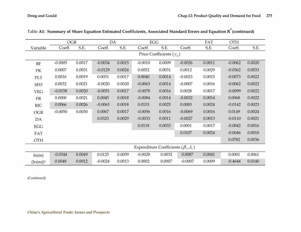
Dong and Gould Chap.12: Product Quality and Demand for Food 275
China's Agricultural Trade: Issues and Prospects
Table A1: Summary of Share Equation Estimated Coefficients, Associated Standard Errors and Equation R2 (continued)
Variable
OGR DA EGG FAT OTH
Coeff. S.E. Coeff. S.E. Coeff. S.E. Coeff. S.E. Coeff. S.E.
Price Coefficients ( ij )
BF -0.0005 0.0017 -0.0034 0.0015 -0.0010 0.0009 -0.0026 0.0011 -0.0062 0.0020
PK 0.0007 0.0031 -0.0129 0.0024 0.0052 0.0031 0.0012 0.0029 -0.0362 0.0033
PLT 0.0016 0.0019 0.0031 0.0017 0.0040 0.0014 -0.0023 0.0015 -0.0073 0.0022
SFD 0.0032 0.0021 -0.0020 0.0020 -0.0063 0.0014 -0.0007 0.0016 -0.0062 0.0022
VEG -0.0158 0.0020 -0.0051 0.0017 -0.0078 0.0016 0.0028 0.0017 -0.0099 0.0022
FR 0.0000 0.0021 0.0045 0.0018 -0.0084 0.0014 -0.0032 0.0014 0.0068 0.0022
RIC 0.0066 0.0026 -0.0063 0.0018 0.0153 0.0025 0.0083 0.0024 -0.0142 0.0023
OGR -0.0050 0.0030 0.0067 0.0017 -0.0056 0.0016 -0.0069 0.0016 0.0149 0.0024
DA 0.0323 0.0029 -0.0033 0.0011 -0.0027 0.0013 -0.0110 0.0021
EGG 0.0118 0.0033 0.0001 0.0017 -0.0042 0.0016
FAT 0.0107 0.0024 -0.0046 0.0018
OTH 0.0782 0.0036
Expenditure Coefficients ( ii , )
ln(m) -0.0344 0.0049 0.0125 0.0059 -0.0028 0.0032 0.0087 0.0041 0.0001 0.0061
(ln(m))2 0.0048 0.0012 -0.0024 0.0013 0.0002 0.0007 -0.0007 0.0009 -0.4644 0.0140
(Continued)

Dong and Gould Chap.12: Product Quality and Demand for Food 276
China's Agricultural Trade: Issues and Prospects
Table A1: Summary of Share Equation Estimated Coefficients, Associated Standard Errors and Equation R2 (continued)
Variable
BF PK PLT SFD VEG FR RIC
Coeff. S.E. Coeff. S.E. Coeff. S.E. Coeff. S.E. Coeff. S.E. Coeff. S.E. Coeff. S.E.
Demographic Characteristics ( isi , )
Intercept 0.0619 0.0106 0.0421 0.0117 0.0451 0.0084 0.0003 0.0106 0.0688 0.0091 0.0768 0.0097 0.0419 0.0094
1/HH_SIZE
0.0076 0.0062 0.0279 0.0071 0.0051 0.0050 0.0062 0.0060 -0.0038 0.0048 0.0040 0.0050 -0.0143 0.0046
Ln(HH_INC)
0.0026 0.0010 -0.0047 0.0012 -0.0007 0.0008 -0.0040 0.0010 -0.0033 0.0008 0.0082 0.0009 -0.0095 0.0008
D_SENIOR
-0.0020 0.0013 0.0015 0.0013 0.0004 0.0009 -0.0005 0.0011 0.0007 0.0010 -0.0040 0.0012 0.0035 0.0010
D_LT_6 -0.0008 0.0017 -0.0026 0.0018 -0.0035 0.0013 -0.0008 0.0017 -0.0051 0.0014 -0.0001 0.0016 -0.0043 0.0016
D_6_14 0.0012 0.0011 -0.0003 0.0012 -0.0017 0.0009 -0.0018 0.0011 -0.0022 0.0010 0.0009 0.0011 -0.0026 0.0010
D_REFRIG
0.0039 0.0012 -0.0018 0.0014 -0.0008 0.0010 0.0019 0.0015 -0.0021 0.0010 0.0036 0.0012 -0.0021 0.0010
D_ GD 0.0072 0.0022 -0.0075 0.0028 0.0142 0.0017 0.0188 0.0019 0.0078 0.0020 -0.0096 0.0022 0.0176 0.0027
D_JS 0.0013 0.0017 0.0005 0.0020 0.0003 0.0013 0.0143 0.0015 0.0045 0.0015 -0.0075 0.0016 0.0214 0.0021
D_HN -0.0029 0.0016 0.0083 0.0018 -0.0027 0.0012 -0.0188 0.0025 0.0109 0.0014 0.0031 0.0016 0.0058 0.0021
D_HLJ 0.0057 0.0016 0.0014 0.0020 -0.0169 0.0014 -0.0091 0.0018 0.0148 0.0014 0.0118 0.0015 0.0221 0.0020
Ln(AGE) -0.0099 0.0027 0.0053 0.0027 -0.0073 0.0021 0.0032 0.0026 0.0093 0.0022 -0.0074 0.0023 0.0064 0.0022
R2 0.088 0.029 0.291 0.385 0.081 0.195 0.231
(Continued)

Dong and Gould Chap.12: Product Quality and Demand for Food 277
China's Agricultural Trade: Issues and Prospects
Table A1: Summary of Share Equation Estimated Coefficients, Associated Standard Errors and Equation R2 (continued)
Variable
OGR DA EGG FAT OTH
Coeff. S.E. Coeff. S.E. Coeff. S.E. Coeff. S.E. Coeff. S.E.
Demographic Characteristics ( isi , )
Intercept 0.0285 0.0099 0.0171 0.0105 0.0382 0.0054 0.0162 0.0063 0.5632 0.0132
1/HH_SIZE -0.0488 0.0058 0.0294 0.0062 0.0001 0.0031 -0.0008 0.0035 -0.0125 0.0067
Ln(HH_INC) -0.0070 0.0009 0.0117 0.0010 -0.0021 0.0005 -0.0066 0.0006 0.0154 0.0011
D_SENIOR 0.0009 0.0012 -0.0003 0.0013 0.0005 0.0006 0.0007 0.0007 -0.0015 0.0015
D_LT_6 -0.0028 0.0014 0.0101 0.0016 -0.0002 0.0008 0.0002 0.0009 0.0099 0.0019
D_6_14 0.0012 0.0011 0.0037 0.0012 0.0001 0.0006 -0.0014 0.0006 0.0030 0.0013
D_REFRIG -0.0068 0.0010 0.0042 0.0015 -0.0017 0.0006 -0.0031 0.0006 0.0047 0.0014
D_ GD -0.0087 0.0025 -0.0201 0.0023 -0.0120 0.0016 0.0010 0.0015 -0.0089 0.0025
D_JS -0.0252 0.0018 -0.0076 0.0015 -0.0079 0.0008 0.0031 0.0010 0.0027 0.0017
D_HN 0.0156 0.0014 -0.0120 0.0018 -0.0025 0.0006 0.0087 0.0008 -0.0134 0.0018
D_HLJ -0.0046 0.0015 -0.0090 0.0016 -0.0045 0.0008 0.0057 0.0010 -0.0174 0.0018
Ln(AGE) 0.0110 0.0024 -0.0099 0.0024 0.0011 0.0013 0.0018 0.0015 -0.0036 0.0031
R2 0.436 0.144 0.332 0.186 0.073
Note: The values that are shaded identify coefficients that are statistically significant at the 0.01 level.

Dong and Gould Chap.12: Product Quality and Demand for Food 278
China's Agricultural Trade: Issues and Prospects
Table A2: Summary of Unit Value Estimated Coefficients, Associated Standard Errors and Equation R2
Variable
BF PK PLT SFD VEG FR RIC
Coeff. S.E. Coeff. S.E. Coeff. S.E. Coeff. S.E. Coeff. S.E. Coeff. S.E. Coeff. S.E.
Demographic Characteristics
Intercept 2.9264 0.082 2.1889 0.0191 2.1824 0.0515 1.4680 0.0602 -0.4922 0.0496 -0.2459 0.0598 0.5713 0.0289
Ln(HH_SIZE)
0.0444 0.0349 0.0232 0.009 0.0368 0.0235 0.0967 0.0284 0.0785 0.0228 0.0327 0.0254 -0.0095 0.0130
Ln(FAH) 0.0925 0.0213 0.0589 0.0048 0.1394 0.0127 0.2501 0.0150 0.2868 0.0126 0.2538 0.0150 0.0713 0.0074
ADVANCE
0.0417 0.0232 0.0171 0.0053 0.0271 0.0139 0.0583 0.0167 0.0159 0.0141 0.0518 0.0167 -0.0057 0.007
LHS 0.0228 0.0207 -0.0137 0.0049 -0.0629 0.0126 -0.0855 0.0158 -0.1047 0.0134 -0.0761 0.0145 -0.0277 0.0069
PER_6_14
0.0357 0.0632 0.0144 0.0147 0.1282 0.0361 0.1049 0.0454 0.2692 0.0394 0.2186 0.0454 0.0259 0.0196
PER_SENIOR
0.0813 0.0294 -0.0112 0.008 -0.0276 0.0204 0.0091 0.0251 -0.1019 0.0205 -0.0979 0.0226 -0.0138 0.0137
PER_LT_6
0.1981 0.1041 0.0039 0.0227 0.0299 0.0580 0.1891 0.0779 0.3602 0.0572 0.4665 0.0743 0.0714 0.0316
D_ GD 0.5244 0.0323 0.3159 0.0078 0.1452 0.0264 0.2228 0.0267 0.5178 0.0282 1.0053 0.0270 0.3383 0.0105
D_JS 0.4695 0.0260 0.0352 0.0070 -0.1192 0.0204 0.1196 0.0207 0.1887 0.0210 0.0253 0.0212 -0.0612 0.0137
D_HN -0.1713
0.0317 0.0075 0.0074 -0.1402 0.0187 -0.1525 0.0224 -0.2152 0.0227 -0.2704 0.0236 -0.0108 0.0110
D_HLJ -0.2442
0.0287 -0.0223 0.0063 -0.2170 0.0156 -0.0807 0.0196 0.0074 0.0181 0.3117 0.0216 -0.0151 0.0108
R2 0.373 0.624 0.295 0.356 0.599 0.688 0.527
(Continued)

Dong and Gould Chap.12: Product Quality and Demand for Food 279
China's Agricultural Trade: Issues and Prospects
Table A2: Summary of Unit Value Estimated Coefficients, Associated Standard Errors and Equation R2 (continued)
Variable
OGR DA EGG FAT OTH
Coeff. S.E. Coeff. S.E. Coeff. S.E. Coeff. S.E. Coeff. S.E.
Demographic Characteristics
Intercept 0.6386 0.0633 4.1023 0.0704 1.3766 0.0236 1.7807 0.0385 3.8278 0.0562
Ln(HH_SIZE)
-0.0353 0.0284 -0.0315 0.0287 0.0134 0.0102 -0.0107 0.0165 -0.1433 0.0243
Ln(FAH) 0.1403 0.0157 0.1798 0.0174 0.0322 0.0059 0.1125 0.0106 0.3106 0.0139
ADVANCE 0.0440 0.0159 0.0254 0.0195 0.0138 0.0060 0.0249 0.0106 0.0740 0.0147
LHS -0.1265 0.0149 -0.0598 0.0171 -0.0002 0.0058 -0.0326 0.0097 -0.0071 0.0134
PER_6_14 0.3443 0.0439 0.1388 0.0468 -0.0039 0.0169 0.0126 0.0275 -0.0009 0.0425
PER_SENIOR
-0.1310 0.0255 -0.0503 0.0245 -0.0119 0.0098 -0.0023 0.0146 0.0365 0.0207
PER_LT_6 0.3410 0.0695 0.3258 0.0761 0.0648 0.0259 0.0370 0.0471 0.1610 0.0655
D_ GD 0.8306 0.0276 -0.1597 0.0306 0.3160 0.0096 0.1965 0.0154 -0.2222 0.0221
D_JS 0.3246 0.0216 -0.0314 0.0285 0.1086 0.0092 -0.1777 0.0117 -0.1423 0.0186
D_HN -0.1289 0.0283 -0.0085 0.0265 0.0287 0.0102 -0.0493 0.0123 0.0639 0.0224
D_HLJ 0.0989 0.0221 -0.0782 0.023 0.0196 0.0093 -0.3862 0.0136 -0.0095 0.0187
R2 0.567 0.082 0.484 0.556 0.265
Note: The values that are shaded identify coefficients that are statistically significant at the 0.01 level.

Lohmar and Hansen Chap.13: Water Scarcity and China’s Agricultural Economy 280
China's Agricultural Trade: Issues and Prospects
Chapter 13:
Interactions between Resource Scarcity and Trade Policy: The Potential Effects of Water Scarcity on China’s
Agricultural Economy under the Current TRQ Regime
BRYAN LOHMAR JAMES HANSEN
United States Department of Agriculture,
Economic Research Service, Washington, DC

Lohmar and Hansen Chap.13: Water Scarcity and China’s Agricultural Economy 281
China's Agricultural Trade: Issues and Prospects
Chapter 13:
Interactions between Resource Scarcity and Trade Policy: The Potential Effects of Water Scarcity on China’s
Agricultural Economy under the Current TRQ Regime*
Introduction
China is facing acute problems managing water resources. Falling ground-water tables and
disruption of surface-water deliveries to important industrial and agricultural regions have
raised concern that a more dramatic crisis is looming unless effective water conservation
policies can be put into place rapidly. Water shortages are confined to a relatively limited
geographic area in northern China which is a major production area for wheat, corn and
cotton.1 China is among the world‘s largest producers and consumers of these crops and
current production levels in northern China rely heavily on supplemental irrigation. A variety
of policies to improve water management and encourage conservation are being established in
China but to date there is little macro-level evidence that these policies are effective. The
success or failure of water management reforms could have significant implications for China‘s
production, consumption and international trade in these commodities.
This chapter provides an overview of how water scarcity could affect China‘s agricultural
production and trade. It provides both a detailed description of water scarcity issues in China
augmented by results from modeling scenarios of water shortages in northern China under
current trade policies. The chapter identifies the areas in northern China where available water
resources are most overexploited, the nature of the threat to water resources for agriculture, and
the crops most vulnerable to reductions in irrigation in that region. We review, and briefly
comment on, the limited research on the impact of water scarcity on agricultural production
and trade in China to date. To contribute to the research findings, we use the Economic
Research Service (ERS) China model to examine scenarios of falling irrigation water availability
in northern China and estimate the effect this will have on China‘s overall production,
* The views expressed are those of the authors and do not necessarily correspond to the views or policies of Economic Research Service, United States Department of Agriculture. 1 Southern China and far northeastern China have relatively abundant water resources, except during infrequent periodic droughts.

Lohmar and Hansen Chap.13: Water Scarcity and China’s Agricultural Economy 282
China's Agricultural Trade: Issues and Prospects
consumption and trade of wheat, corn and cotton. The ERS China model is a detailed
agricultural partial equilibrium dynamic simulation model and is part of the Country-
Commodity Linked System (CCLS) of 38 countries and regions used for annual United States
Department of Agriculture‘s (USDA) Long-term projections.
Our findings indicate that China‘s large agricultural economy has substantial capacity to
adapt to production decreases in the water-short north by increasing production in other parts
of China, decreasing consumption as well as increasing imports. Under China‘s current trade
regime of tariff-rate quotas (TRQs) for these commodities, declining production in northern
China will increase prices and increase demand for imports, but the demand for imports will be
partially offset by increased production in less water-stressed parts of China. Higher prices will
also induce consumption decreases as China still has many low-income consumers who are
price sensitive. Thus, even under scenarios of large decreases in irrigated area in the north,
imports rise much less than the induced production shortfalls. The role of China‘s TRQ regime
for imports is critical in maintaining relatively inelastic import demand that serves to drive
prices up as production declines in the north yet reduce demand for imports as a means to
adjust to production shortfalls.
Water Scarcity and Irrigated Agriculture in China
China, overall, is moderately well endowed with water but the water is unevenly distributed
geographically. As with arable land, China‘s total water resources are close to those of the
United States, roughly 2,800 billion cubic meters (bm3) of total exploitable water resources per
year (FAO). However, having a much larger population, China‘s per-capita water resources are
roughly 2,200 m3, about one quarter that of the United States, which is close to the world
average. Still, China‘s overall per capita water endowment is well above water scarce
endowment levels which tend to range between 1,500-1,700 m3 per capita for moderate water
scarcity (Liu, 1998). Similar to the United States, China‘s water is disproportionately
distributed: areas south of and including the Chang (Yangtze) River Basin, and in the far
northeast, contain about 90% of China‘s water. The productive agricultural areas in northern
China, however, possess only about one tenth the world levels of water per capita and are well
below international standards for water scarcity on a per capita basis. Agriculture is most
threatened by water scarcity in the area commonly referred to as the North China Plain, the
productive grain belt centered in northern Henan and Shandong and southern Hebei Provinces.
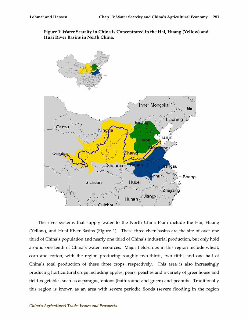
Lohmar and Hansen Chap.13: Water Scarcity and China’s Agricultural Economy 283
China's Agricultural Trade: Issues and Prospects
Figure 1: Water Scarcity in China is Concentrated in the Hai, Huang (Yellow) and Huai River Basins in North China.
The river systems that supply water to the North China Plain include the Hai, Huang
(Yellow), and Huai River Basins (Figure 1). These three river basins are the site of over one
third of China‘s population and nearly one third of China‘s industrial production, but only hold
around one tenth of China‘s water resources. Major field-crops in this region include wheat,
corn and cotton, with the region producing roughly two-thirds, two fifths and one half of
China‘s total production of these three crops, respectively. This area is also increasingly
producing horticultural crops including apples, pears, peaches and a variety of greenhouse and
field vegetables such as asparagus, onions (both round and green) and peanuts. Traditionally
this region is known as an area with severe periodic floods (severe flooding in the region

Lohmar and Hansen Chap.13: Water Scarcity and China’s Agricultural Economy 284
China's Agricultural Trade: Issues and Prospects
occurred as late as the 1960s), but increasing water diversions for agriculture, industry and
urban domestic use has greatly reduced river flows and the potential for floods. Year-to-year
rainfall variability, coupled with the concentration of the region‘s rainfall in the late summer
months (roughly 70%of rainfall in the North China Plain falls in July, August and September),
leaves open the possibility of local flooding during this period despite the stresses caused by the
heavy exploitation of water resources.
The Hai River Basin is an area where water shortages are most severe. The Hai River Basin,
centered on Hebei Province, refers to a number of tributaries that flow into a short sea channel
in Tianjin known as the Hai River (Figure 1, green area). Underlying this surface water
structure is a complex set of overlapping aquifers, with varying recharge rates. Major urban
areas in the Hai River Basin are drawing down the groundwater table to an extent that many
have experienced land subsidence as a result.2 On top of rising urban demand, irrigated area
has increased over the last 40 years due to widespread establishment of tube-wells powered by
electric or diesel pumps. The number of tube-wells in China grew from 150 thousand in 1965 to
more than 2.3 million by the late 1970s, with most of these concentrated on the North China
Plain (Shi, 2000), and this number has most likely risen dramatically since that time. The
expansion of irrigation not only has allowed for higher yields, but also allows farmers to double
crop, generally winter wheat followed by corn. The Hai River Basin became a major wheat-
producing region as irrigated area increased. Extensive irrigation, coupled with urban and
industrial demand for water, have drawn down the water tables throughout the basin at
increasing rates, exceeding three meters per year in some rural regions in the 1990s (Wang and
Huang, 2002). Exploitation of the groundwater is most severe in the central part of the Basin,
and saltwater intrusion and poor drainage are causing salinization in the center and eastern
parts of the region. Surface water is also over-exploited. Cangzhou, a downstream prefecture
in Hebei Province, receives less than 10%of the surface water deliveries received in the 1970s
(Lohmar and Crook, 2002). Similar examples of overexploited surface water resources can be
found throughout the basin.
Water resources in the Yellow River Basin also show signs of over-exploitation. The Yellow
River meanders from its headwaters on the edge of the Tibetan Plateau in Qinghai Autonomous
Region, turns north through the steppe and desert provinces and autonomous regions of Gansu,
2 In addition to Beijing (population 13 million) and Tianjin (population 9 million), there are three other cities with urban populations over 1 million and five with urban populations between 500,000 and 1 million in the basin.

Lohmar and Hansen Chap.13: Water Scarcity and China’s Agricultural Economy 285
China's Agricultural Trade: Issues and Prospects
Ningxia and Inner Mongolia, turns south along the Shaanxi and Shanxi Provincial border, then
turns east again and towards the ocean through northern Henan and Shandong Provinces
(Figure 1, in yellow). A few large upstream irrigation districts in Gansu, Ningxia and Inner
Mongolia developed over the last few decades now draw off large amounts of water to irrigate
agricultural areas that are substantially less productive than downstream areas. Upstream
areas increasingly exploit their access to water for industrial development as well. Since the
early-1970s, water in the Yellow River has often been drawn off to such an extent that the river
did not flow into the ocean for part of the year. In 1997 and 1998, over-exploitation was
particularly acute, the river did not reach the ocean for over 220 days in both years, and the dry
stretch reached as far as 700 kilometers inland (Liu, 1998; Liu, 1999). When this happens,
farmers in the productive downstream provinces of Shandong and Henan are denied surface
water for part of the irrigation season. Since 1999, however, the river has been more tightly
managed so that it does not run dry, but downstream sluice gates leading to irrigation districts
may be abruptly closed when the river flow reaches a minimum threshold in those areas (this
minimum threshold is often referred to as environmental flow).
The Huai River Basin also suffers from poor drainage and acute pollution, in addition to
over-exploitation and water shortages during dry periods. For roughly 700 years prior to 1857,
the Yellow River flowed to the East China Sea through this region, and built up large deposits
of silt, ultimately causing it to change course for its current route through Shandong to the
north. However, the silt deposits left by the Yellow River obstructed the drainage from the
tributaries that remained primarily the Huai River, but also the many smaller rivers and
tributaries in the basin. Thus, much of the drainage in this region does not flow directly into the
ocean. Instead the main water flow is into Hongze Lake, where it then is diverted south to the
Yangtze River. In the past few decades, a man-made channel has been built to divert some
Huai River water directly to the East China Sea, and some gets diverted to the former Grand
Canal, which serves to bring water from the Yangtze to more arid northern Jiangsu (and will
ultimately comprise the eastern route of China‘s South-North water transfer program). Because
of the siltation, drainage as well as water shortages are a problem in this basin, and periodic
floods still occur after incidences of severe rainfall. However, even in normal years, water
resources in this region are heavily taxed by the large population and extensive irrigation, and
surface water sources may dry-up or become unusable for irrigation.

Lohmar and Hansen Chap.13: Water Scarcity and China’s Agricultural Economy 286
China's Agricultural Trade: Issues and Prospects
Irrigation in this region allows farmers to not only increase yields but also plant two crops a
year. Precipitation on the North China Plain is unevenly distributed throughout the year, with
70% of the rainfall arriving in the three-month period from July-September. Single season corn
and summer sown cotton can be grown in this period without supplemental irrigation. With
irrigation, however, farmers can grow a second crop in the spring, usually winter wheat, and
still realize satisfactory yields. Winter wheat is irrigated roughly 4-5 times, once in the fall after
planting, then 3-4 times in the spring when rainfall is low, and is harvested in June. If rainfall is
still low after planting corn in late June, and if water is available, farmers may also irrigate corn
or whatever second crop they choose to grow, to get the seedlings started, but the bulk of corn
production occurs during the period with adequate rainfall. Spring-sown cotton in the North
China Plain also relies on supplemental irrigation in the spring, but can withstand a dry spell
before the rainy season.
Understanding these features of China‘s water issues is important for understanding how
water scarcity may affect China‘s agricultural economy. Water scarcity in China is extremely
localized. Most of China has sufficient water, and some of China has too much water so that
flooding and drainage issues take priority over conservation. But in areas in and around the
North China Plain, water resources are scarce on both a per capita and per land basis. Largely
because of the regional aspect of water scarcity in China, increasingly stressed water resources
affects some crops more than others. For example, China‘s overall production of rice and
soybeans is less sensitive to water stress because only a small percentage of those crops are
produced in water-stressed regions. But major shares of China‘s wheat, corn, and cotton crops
are produced in the regions facing water scarcity, thus are more exposed to a deterioration of
the water availability for agriculture. Moreover, even among these crops there are important
differences, with some crops being more or less vulnerable to disruptions in supplemental
irrigation than others. Since the primary growing season for winter wheat is in the spring, and
the primary rainfall season is in the late summer (July-September), wheat relies heavily on
supplemental irrigation. Other crops, such as corn and cotton, grow primarily during the late-
summer, intensive-rainfall, months and are less sensitive to supplemental irrigation unless there
are droughts, which occur with some frequency in the region.

Lohmar and Hansen Chap.13: Water Scarcity and China’s Agricultural Economy 287
China's Agricultural Trade: Issues and Prospects
Estimation of the Implications for Agriculture
There are a few published estimates of how water shortages will affect agricultural production
in China (Table 1). Modeling approaches vary in these estimates and include a hydro-climatic
approach (Heilig et al., 2000), a hydrological-economic approach with varying water prices
(Rosegrant and Cai, 2002), extrapolation of water use and water efficiency trends (Yang and
Zender, 2000), and results from a simulation model using econometrically estimated parameters
(Huang et al., 2007). In addition, the results vary widely, even within the same study. For
example, Heilig et al. predict that at current levels of water use efficiency, China‘s grain
production will fall short of projected demand by 156 million metric tonnes (mmt) in 2025, but
that with increased efficiency, grain production can exceed projected demand by 22 mmt in that
year. Rosegrant and Cai‘s (2002) results show a more moderate effect. They predict that China
will import 47.2 mmt of grain in 2025 as a baseline and this figure rises to 56.7 mmt under a
scenario where water prices are tripled. Under a scenario where water use efficiency increases
in addition to the higher water prices, imports fall back to below the baseline, to 46.3 mmt.
Huang et al. find that with prices rising to level 50% greater than the current marginal value of
water in agriculture, wheat production in north China will fall by nearly 20 mmt.
While these studies provide insight into how China‘s agricultural sector may respond to
water shortages, there are a number of shortcomings with the analysis. A primary shortcoming
with most previous work is that they often take China as a whole (Heilig et al., 2000; Rosegrant
and Cai, 2002), but water scarcity is very much a regional phenomenon. Moreover, most
studies provide long-term projections (more than 20 years) of China‘s agricultural supply and
demand which have been unreliable in the past. For example, projections made in past decades
predicted that China would import corn, and none predicted that China would still be
exporting corn in 2007.

Lohmar and Hansen Chap.13: Water Scarcity and China’s Agricultural Economy 288
China's Agricultural Trade: Issues and Prospects
Table 1: Previous Studies into the Effects of Water Scarcity on China’s Agricultural Trade
Reference Modeling Approach Conclusions
Brown and Heilwell (1998)
Cites modeling sponsored by the US National Intelligence Council
China imports 175 mmt grain by 2025, and over 200 mmt by 2030
Heilig, Fischer and Van Velthuizen (2000)
Use hydro-climatic model to show that agricultural production is sustainable at current levels and with current technology, but will not keep up with increases in demand.
Find China will produce roughly 156 mmt less than estimated demand in 2025 with current irrigation levels, but has a maximum production potential of 22 mmt above the estimated demand in 2025 if irrigation is expanded.
Yang and Zender (2001)
Extrapolate from current trends of water use and increases in water use efficiency.
Recommends China import 10 mmt of wheat to relieve over-exploitation of water
Rosegrant and Cai (2002)
Use hydrological-economic model linked to IFPRI‘s IMPACT model to estimate how changes in water prices and water use efficiency in China affect international trade.
Find that China will import 56.7 mmt of grain in 2025 if water prices are tripled, 9.5 mmt higher than the baseline of 47.2 mmt (without raising water prices). Imports fall to 46.3 mmt if water use efficiency increases and water prices rise.
Lohmar and Hansen Chap.13: Water Scarcity and China’s Agricultural Economy 289
China's Agricultural Trade: Issues and Prospects
An additional, and related, shortcoming in some of these studies is that they aggregate
grains, concealing different trends in food grains, feed grains and other crops. Rising incomes
and urbanization are generating more diversified diets in China, increasing the consumption of
livestock products, while decreasing per capita consumption of food grains like rice and wheat.
Thus, demand for feed grains such as corn is expected to rise dramatically over the next few
decades as China‘s per capita consumption of livestock products increases with income. Corn,
however, is less threatened by unreliable irrigation because it is grown in the rainy season,
while wheat relies heavily on supplemental irrigation. In addition, studies have not addressed
the effects of water scarcity on cotton, also an important crop in north China. Demand for
cotton in China has increased dramatically after the Multi-Fiber Arrangement (MFA) ended at
the end of year 2004, but cotton is rarely considered in estimates of water scarcity and
agricultural trade.
In our model, we add parameters to address some of these issues described above. In order
to see how regional water scarcity might affect China‘s overall agricultural economy, we
estimated the effects of a decrease in irrigated area in northern China using the China model
that is incorporated into the ERS CCLS. The CCLS is a partial equilibrium model of the world
agricultural economy used to provide the annual USDA Long-term projections. The model
solves for international supply and demand for 24 commodities in 38 countries and regions, and
a major part of the CCLS is a model of China‘s agricultural economy. Using the China model
allows us to determine how international markets for each crop are affected by water shortage
scenarios. The China model is disaggregated into six regions. We focus on the northern region
which includes five agricultural provinces (Hebei, Henan, Shandong, Shanxi, Shaanxi and Inner
Mongolia) and two metropolitan centers (Beijing and Tianjin). This region is where agricultural
production is most threatened by water scarcity.
The scenarios focus on wheat, corn and cotton production in northern China. We make
assumptions regarding the difference between irrigated and non-irrigated yields for these three
crops during an average rainfall year in northern China. These assumptions are based on
interviews carried out by the authors over the last 5 years, as well as econometric findings from
data collected in this region by the Chinese Academy of Sciences (CAS). We used findings
The assumptions on irrigated and non-irrigated yields, as well as on irrigated area by crop in this region, are derived from a five-year collaboration between USDA-ERS, China‘s Ministry of Water Resources, the Center for Chinese Agricultural Policy (CCAP), the Australian Bureau of Agricultural and Resource Economics, and the

Lohmar and Hansen Chap.13: Water Scarcity and China’s Agricultural Economy 290
China's Agricultural Trade: Issues and Prospects
from survey work in Northern China, also conducted by CAS, on the irrigated area by crop to
calculate an adjusted weighted average of the yields that matches the yields for each crop used
in the base year of the 2007 USDA Long-term projections.
Using the modified model, we estimated a series of scenarios by reducing the amount of
irrigated land in northern China over the projection period. The 4 scenarios estimated the
effects of a decline in total irrigated land in northern China of 10, 20, 30 and 40% over the 10-
year projection period. These scenarios are intended to approximate the effect of a reduction in
water allocated to agriculture over the period, and estimate how agriculture will change in the
region if water for irrigation is reduced. The model provides estimates of total irrigated crop
production in northern China, total non-irrigated crop production in northern China,
production in other regions of China, price changes, consumption, imports and exports. By
comparing the results of these scenarios to the 2007 USDA Long-term projections for year
2015/2016, we estimate how falling irrigation in northern China might affect China‘s broader
agricultural economy.
The 2007 USDA Long-term projections were generated based on policies currently in place.
The forecasts assume the continuation of China‘s TRQ import regime for the three commodities.
China‘s TRQ regime was adopted upon WTO accession in 2001 and sets a share of each quota
aside for non state-trading enterprises, with the remainder of the TRQ under the control of
China‘s state-owned import-export companies (heretofore, state-trading enterprises). For
example, for wheat the TRQ amount is 9.8 mmt, but 90% of this is set-aside for state-trading
enterprises. This unique TRQ regime is modelled by assuming differing import elasticities for
state and non-state shares. For the non-state share of the TRQ, the import response to domestic
price changes is more elastic than the import response for the state-share of the TRQ. We also
assume the non-state and state shares of the TRQ are filled sequentially. As prices increase,
imports occur first with the more-elastic non-state share. When the non-state share of the TRQ
fills, import demand becomes less elastic as state enterprises begin to import. Once the TRQ
fills, imports face higher over-quota tariffs of 40% for corn and cotton and 65% for wheat,
compared to in-quota tariffs of just 1%for the three commodities (Lohmar et. al, 2002).4
University of California at Davis. CCAP conducted extensive fieldwork and data collection in this region, and USDA-ERS received access to these data as part of our participation in the collaboration. 4 Recently, China has been importing cotton at level above the TRQ but charging a sliding scale tariff rather than the above quota tariff of 40%. The sliding scale tariff starts at 5%, and goes higher as imports increase.
Lohmar and Hansen Chap.13: Water Scarcity and China’s Agricultural Economy 291
China's Agricultural Trade: Issues and Prospects
We provide important insights into how water scarcity might affect China‘s overall
agricultural economy by modeling how production changes in one region affect another region
in China. We find that water scarcity may induce significant production declines in northern
China, but the effects of these declines will be partially offset by supply response in other
regions, reducing the demand for imports. This happens, at least in part, because of China‘s
TRQ regime and the extent to which it discourages imports.5
Results
The results from the modeling indicate that production declines in northern China due to
reduced irrigation may raise domestic prices and induce increased production in other regions
of China under the TRQ regime. Higher prices would also reduce consumption of these
commodities. The extent to which water scarcity in China results in higher domestic prices
depends on China‘s import policies, which dampens import response and cause prices to rise
more than under less restrictive import regimes.
Wheat: Because of the reliance on supplemental irrigation in northern China, wheat is the
crop that is most affected by declining access to irrigation. Figure 2 shows the effect of four
different scenarios on production in northern China, production in other parts of China,
national consumption and net imports of wheat. Model results were produced for scenarios in
which irrigated area falls 10, 20, 30 and 40%. The production of wheat in northern China falls
by only 2.1 mmt when irrigated area falls by 10% (about 2.3% of China‘s total wheat production
estimated by USDA Long-term projections for the crop year 2015/6). However, production falls
by nearly 18.3 mmt when irrigated area falls by 40%. For the most part, we anticipate that
farmers will simply go out of wheat production when they lose access to irrigation, but some
(very few) farmers will maintain rain-fed wheat production when irrigation access is lost.
The production shortfalls in northern China cause prices to rise and this, in turn, causes
wheat production in other regions to increase. Thus, the total decline in wheat production in
China is smaller than the decline in the North China Plain and adjacent water scarce regions.
For example, when irrigated area declines by 10%in northern China, the production in the north
falls by 4.5 mmt, but production in other parts of China increases by 2.1 mmt, resulting in
China‘s total wheat production falling by only 2.4 mmt (Figure 2). With the larger 40% fall in
irrigated area, production in the north falls by 18.3 mmt, but increases in other areas by 6.4
5 Subsequent research will examine the welfare effects of increasing water scarcity under China‘s TRQ, and compare to scenarios with more liberal trade regimes.
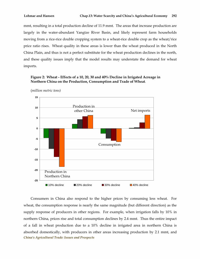
Lohmar and Hansen Chap.13: Water Scarcity and China’s Agricultural Economy 292
China's Agricultural Trade: Issues and Prospects
mmt, resulting in a total production decline of 11.9 mmt. The areas that increase production are
largely in the water-abundant Yangtze River Basin, and likely represent farm households
moving from a rice-rice double cropping system to a wheat-rice double crop as the wheat/rice
price ratio rises. Wheat quality in these areas is lower than the wheat produced in the North
China Plain, and thus is not a perfect substitute for the wheat production declines in the north,
and these quality issues imply that the model results may understate the demand for wheat
imports.
Figure 2: Wheat - Effects of a 10, 20, 30 and 40% Decline in Irrigated Acreage in Northern China on the Production, Consumption and Trade of Wheat. (million metric tons)
-25
-20
-15
-10
-5
0
5
10
15
10% decline 20% decline 30% decline 40% decline
Production in other China
Consumption
Net imports
Production in Northern China China
Consumers in China also respond to the higher prices by consuming less wheat. For
wheat, the consumption response is nearly the same magnitude (but different direction) as the
supply response of producers in other regions. For example, when irrigation falls by 10% in
northern China, prices rise and total consumption declines by 2.4 mmt. Thus the entire impact
of a fall in wheat production due to a 10% decline in irrigated area in northern China is
absorbed domestically, with producers in other areas increasing production by 2.1 mmt, and
Lohmar and Hansen Chap.13: Water Scarcity and China’s Agricultural Economy 293
China's Agricultural Trade: Issues and Prospects
consumers decreasing consumption by 2.4 mmt, and together these offset the 4.5 mmt
production decline in northern China. Larger irrigated area declines in northern China,
however, bring about much larger production declines and the combined effects of production
and consumption do not cover these declines. When production in north China falls by 18.3
mmt under the scenario of 40% decline in irrigated acreage, consumption falls by 6.4 mmt. This
again is about the same as the rise in production in other regions (also rounded to 6.4 mmt) but
together only comprise 12.8 mmt. The remaining shortfall is made up by (net) imports, which
increase by 6.4 mmt as well.
The responses of producers in other regions, consumers and imports are due largely to
restrictive trade policies that impede imports and allow domestic prices to rise well above the
prices on international markets. Wheat has the most restrictive import policies of the three
crops we address, with 90% of the TRQ set aside for state-trading enterprises. But the 2007
USDA Long-term projections for China‘s wheat imports in 2015/16 are 3.28 mmt, above the
non-state share of the TRQ, so any additional imports due to water scarcity occur at the more
restrictive state-trading portion of the TRQ. This causes prices for wheat to rise fairly rapidly as
irrigated acreage declines in northern China, and this explains why producers in other regions
increase production and consumers reduce consumption of wheat. When irrigated acreage in
northern China declines by 10%, wheat prices will rise by 19.2% above the baseline projections.
When irrigation in northern China declines by 40%, wheat prices will rise by 62.5% above the
baseline prices.
Corn: The response of the corn market is similar to wheat, but not as pronounced (Figure
3). Like wheat, corn production declines in northern China as irrigated land becomes scarce,
but to a lesser extent. Moreover, as with wheat, production in other regions in China rises,
consumption declines, and these changes dampen China's overall import response. In the
scenario representing the smallest impact, a 10% fall in irrigated area, corn production in
northern China declines by 2.9 mmt, but, similar to wheat, the response of consumers and
producers in other areas results in a non-significant change in imports. Under this scenario,
production in other regions increases by 1.4 mmt and consumption falls by 1.3 mmt, leaving the
remaining 200,000 mt to net imports, roughly half coming from a reduction in exports.

Lohmar and Hansen Chap.13: Water Scarcity and China’s Agricultural Economy 294
China's Agricultural Trade: Issues and Prospects
Figure 3: Corn - Effects of a 10, 20, 30 and 40% Decline in Irrigated Acreage in Northern China on the Production, Consumption and Trade of Corn.
(million metric tons)
-15
-10
-5
0
5
10
10% decline 20% decline 30% decline 40% decline
Production in northern China
Production in other China
Consumption
Net imports
Consumption and production of corn are very responsive to the price changes induced by
the production shortfall in northern China. This leaves corn imports much less responsive to
large production shortfalls on the North China Plain. When irrigated acreage decreases by 40%,
corn production in northern China decreases by 10.9 mmt, but producers in other areas increase
production by 5.4 mmt, and consumption declines by 4.9 mmt, so net imports are only 700,000
mt above baseline predictions when water scarcity in northern China is most acute.
Not only does corn production decrease less than wheat, but prices rise less as well. The
lower price response of domestic corn that results from larger regional domestic production
shocks is largely due to the price-responsiveness of consumption and production. Corn prices
rise by 6.7% under the "10% decline in irrigated area" scenario, and rise by 23.8% under the
assumption, "irrigated acreage falls by 40% in northern China", far less than the 19.2% and
62.5% rise in wheat prices under those scenarios. This is because there are very productive
regions in the far northeast that can move into corn production as prices rise (generally by
Lohmar and Hansen Chap.13: Water Scarcity and China’s Agricultural Economy 295
China's Agricultural Trade: Issues and Prospects
replacing soybeans or japonica rice with corn). Also, the demand for livestock products, the
primary user of corn in China, is more price elastic than the demand for staple grains such as
wheat, so the livestock market shrinks somewhat as corn prices rise and this reduces demand
for corn. Livestock producers also likely find substitutes for corn in their feed rations for meat
production as prices rise.
Cotton: As with wheat and corn, increasing water scarcity induces a decline in cotton
production in northern China (Figure 4). But unlike the other two commodities, this decline is
matched largely by imports. As irrigated area falls by 10% in northern China, cotton
production in the region falls by 255,600 mt. This induces a price increase of only 2.6%, causing
consumption to fall by only 76,000 mt. Moreover, since there is little capacity to expand cotton
production in China, production outside of northern China increases by only 15,600 mt. Thus
net imports take up most of the gap by increasing 164,000 mt. Looking at the more severe
scenario of a 40% decline in irrigated area, we find the same pattern: production in the north
falls by 989,000 mt, inducing prices to rise 10.1%, production in other regions to increase by
69,000 mt, consumption to fall by 285,000 mt, and net imports to rise by 634,400 mt.
China‘s cotton market relies more heavily on imports than corn or wheat and is protected
less, resulting in a larger import response as production falls in northern China. In recent years,
China has allowed cotton imports well beyond the TRQ to enter the country at sliding-scale
tariffs that are lower than the stated above-quota tariff of 40%. This is because the demand for
cotton in China surged after the end of the MFA in 2004, allowing China‘s exports of textiles to
boom.
Other Crops: The effects on the wheat, corn and cotton markets from scenarios of declining
irrigation in northern China have second-order spillover effects in other markets. For example,
rice production declines under these scenarios, about 742,000 mt in the ―40% decline‖ scenario.
The decline in rice production is likely due to producers in water-abundant areas substituting
wheat and corn for rice when the prices for these commodities rise. Still, the decline is small
compared to China‘s overall rice crop, only 0.5% of total estimated rice production in 2015/16.
Livestock markets are also affected under these scenarios, likely due to rising corn prices.
Under the severe ―40% decline‖ scenario, pork production declines 1.4% and poultry
production declines 4.4%. The decline in livestock production also induces a decline in soybean
production and imports, by 2.7% and 1.0% respectively. The decline in soybean production also

Lohmar and Hansen Chap.13: Water Scarcity and China’s Agricultural Economy 296
China's Agricultural Trade: Issues and Prospects
may be due to expanding corn production in the northeast region.
Figure 4: Cotton - Effects of a 10, 20, 30 and 40% Decline in Irrigated Acreage in Northern China on the Production, Consumption and Trade of Cotton. (thousand metric tons)
-1500
-1000
-500
0
500
1000
10% decline 20% decline 30% decline 40% decline
Production in northern China
Production in other China
Consumption
Net imports
Caveats: These scenario results provide a snapshot of how China‘s agricultural economy
might adapt to declining water availability for agriculture in and around the productive North
China Plain. However, there are important caveats that should be stated. One is that the nature
of the modeling does not take into account the possibility of increased water use efficiency in
agriculture. It is unclear exactly how increased water use efficiency might affect the water
scarcity problems in north China, particularly in areas using groundwater. Some argue that
water tables are continuing, and will continue, to fall even as water is used more efficiently in
agriculture (Kendy et al., 2003), while others argue that there is substantial capacity to use water
more effectively and curb the deterioration of water resources (Lohmar et al. 2003). The way we
model declining irrigated acreage might be viewed as a ―worst case scenario‖ for the future of
irrigated agriculture in China.

Lohmar and Hansen Chap.13: Water Scarcity and China’s Agricultural Economy 297
China's Agricultural Trade: Issues and Prospects
A second caveat is that while these scenarios look at a sustained deterioration in water
availability for agriculture in China, they do not reflect the effect of periodic droughts.
Droughts in this region can last more than one year and can have devastating effects on crop
production. Corn and cotton are especially vulnerable to droughts since they are often grown in
rainfed areas that have no access to irrigation or less secure access to surface water irrigation
that itself could be affected by a drought. In much of the region, wheat can only be grown with
supplemental irrigation so is produced only where there are secure sources of water, such as
ample ground water, making it less vulnerable to droughts. In areas that receive water from the
Yellow River, the dry periods tend to be in the latter part of the summer growing season. Spring
season flows are relatively secure as the river carries the snowmelt from the Tibetan Plateau.
Thus, surface water in the basin is more secure for wheat production in the spring than it is for
corn and cotton in the late summer.
Conclusion
Over-exploitation of water resources and the changes brought about to adapt to limited water
resources will almost certainly induce changes in China‘s agricultural production patterns.
Increasing urban demand for water as well as demand for environmental flows, such as those to
maintain the Yellow River flows to the ocean, will limit the amount agriculture can continue to
draw off the water system in the important grain producing areas of northern China. But many
of these areas have seen dramatic increases in grain production due to the establishment of
irrigation systems over the last 50 years. With irrigation now threatened and policy no longer
focused on providing cheap irrigation to maintain grain self-sufficiency, changes in agricultural
production are likely to occur. Given China‘s size and importance in the world food system,
these changes will likely affect international markets.
China‘s size, however, also serves to dampen the effects of declines in production in the
northern region on international markets. Because China is such a large producer and
consumer of the crops affected by water shortages in the northern region, there is substantial
capacity for response by domestic consumption and producers in other regions to the shortfalls
in production in the north. Moreover, the magnitude of the changes on international markets
depends on a variety of factors. The success and effectiveness of water policy changes currently
being promoted will make a difference. Trade policy also clearly matters. With more
liberalized trade policies, China‘s adjustment to production shortfalls in the north will more

Lohmar and Hansen Chap.13: Water Scarcity and China’s Agricultural Economy 298
China's Agricultural Trade: Issues and Prospects
likely be via importing ―virtual water‖ – water embodied in crops. Under such circumstances,
prices will increase less, consumers will consume more, and production in other areas will
change less, resulting in an overall welfare gain.
References
Brown, L. and B. Heilwell. ―China‘s Water Shortage Could Shake World Food Security,‖ World
Watch (July/August, 1998). Available at: www.worldwatch.org/mag/1998/98-4a.html. FAO, FAOSTAT, AquaSTAT website. Available at: http://faostat.fao.org/site/544/default.aspx]. Heilig, G., G. Fischer, and H. Van Velthuizen. ―Can China Feed Itself? An Analysis of China‘s
Food Prospects with Special Reference to Water Resources‖, International Journal of Sustainable Development and World Ecology 7(2000): 155-172.
Huang, Q., S. Rozelle, R. Howitt, J. Wang, and J. Huang. ―Irrigation Water Pricing Policy in China,‖ Working Paper (2007). Minneapolis St. Paul: Department of Applied Economics, University of Minnesota.
Kendy, E., D. Molden, T. Steenhuis, C. Liu, and J. Wang. ―Policies Drain the North China Plain: Agricultural Policy and Groundwater Depletion in Luancheng County, 1949-2000,‖ Research Report No. 71 (2003). Colombo, Sri Lanka: International Water Management.
Liu, C. ―Environmental Issues in China‘s South-North Water Transfer Projects,‖ China Quarterly 158(1998): 68-93.
Liu, J. ―Utilization of Land and Water Resources in China: Resource Endowments and Institutional Arrangements.‖ In Agriculture in China and OECD Countries: Past Policies and Future Challenges, Paris: OECD (1999).
Lohmar, B., J. Wang, S. Rozelle, J. Huang and D. Dawe. China’s Agricultural Water Policy Reforms: Increasing Investment, Resolving Conflicts and Revising Incentives, Agricultural Information Bulletin No. 782. Washington DC: Economic Research Service, USDA (2003).
Lohmar, B., J. Hansen, R. Seeley and H. Hsu. ―WTO Accession will Increase China‘s Agricultural Imports,‖ Agricultural Outlook, No. 270. Washington DC: Economic Research Service, USDA (2002).
Lohmar, B. and F. Crook. ―2002 USDA-MOA Scientific Exchange on Water Resources and Agricultural Production, Trip Report.‖ Washington DC: Economic Research Service, USDA (2002).
Rosegrant, M., and X. Cai. ―Market Adaptations to Increased Water Prices in China: the Impact on Water Demand and Rice Production.‖ Paper presented to the 2002 International Rice Conference (September 16-20, 2002). Beijing, China.
Shi, Y. (2000) ―Groundwater Development in China.‖ Paper for the Second World Forum (17–22 March, 2000). The Hague, Netherlands.
Wang, J. and J. Huang. Effective Water Management Institutions in the Fuyang River Basin, China. Final Research Report submitted to International Water Management Institute and Asian Development Bank (2002).
Yang, H., and A. Zender. ―China‘s Regional Water Scarcity and Implication for Grain Supply and Trade,‖ Environment and Planning A 33(2001): 79-95.
Gruère et al. Chap.14: Genetically Modified Rice 299
China's Agricultural Trade: Issues and Prospects
Chapter 14:
Genetically Modified Rice, International Trade, and First-Mover Advantage: The Case of India and China
GUILLAUME GRUÈRE
SIMON MEVEL ANTOINE BOUËT
International Food Policy Research Institute

Gruère et al. Chap.14: Genetically Modified Rice 300
China's Agricultural Trade: Issues and Prospects
Chapter 14:
Genetically Modified Rice, International Trade, and First-Mover
Advantage: The Case of India and China*
Introduction
During the last decade, a number of Asian countries have been actively developing programs of
research on genetically modified (GM) crops (Runge and Ryan, 2004). Some of these countries
have developed biosafety regulatory frameworks, but until now only a few have approved one
or more GM crops. Empirical studies have shown that the introduction of Bt cotton in China
and India have generated income gains for farmers overall (e.g., Bennett et al., 2004, Pray et al.,
2002). But these two countries only approved the large scale production of GM cotton, in part
because unlike other GM crops, the main products of cotton are not used for food, and thus are
not subject to food safety approval and labeling regulations in major importing countries. In
particular, neither Japan nor the European Union (EU) directly regulates textile products
derived from GM cotton.
In fact, most Asian countries that have invested in research and regulations on GM food
crops are confronted with three possible alternatives: 1) allowing the production of GM food
crops with the risk of losing potential exports, 2) rejecting the commercialization of any GM
food crop, 3) producing both GM and non-GM food crops separately at a marketing cost. At the
same time, they have to take into account the potential opportunity cost of rejecting the
technology when other competitors adopt it (Elbehri and MacDonald, 2004; Berwald et al.,
2006). In the last few years, China has been conducting field trials of different varieties of GM
rice but has delayed a decision on its formal approval. At the same time, India has been actively
conducting public research on GM rice, but many officials appear reluctant to see its
introduction. India‘s rice exports to sensitive markets are significant, but non-GM rice
segregation could help preserve its exports while allowing the rest of the country to use GM rice
* The authors wish to thank Rowena Valmonte-Santos, Liang You, Cynthia Rossi, and Purvi Mehta-Bhatt, for their
help and contributions at various stages of the first phase of the project on productivity modeling. They would also like to thank all the participants to the meetings in the five cities in India. This research was supported by the South Asia Biosafety Program, a program managed by the International Food Policy Research Institute and funded by the United States Agency for International Development. Views expressed in this article are the authors‘ alone.

Gruère et al. Chap.14: Genetically Modified Rice 301
China's Agricultural Trade: Issues and Prospects
to increase its agricultural productivity, and therefore help feed a large and fast-growing
population.
This chapter provides an integrated ex-ante economic assessment of these strategies
focusing on the case of GM rice resistant to biotic and abiotic stresses in India with or without
GM rice introduction in China. More specifically, this chapter has three main objectives. First,
we assess the impact of large importers´ regulations on the economic effects of GM rice
adoption in India. Second, we evaluate the opportunity cost of GM/non-GM rice segregation
under the external constraints previously defined. Third, we analyze the economic effects of
GM rice adoption in India before or after China. In 2006, for the first time, India‘s total GM
cotton area surpassed China‘s (James, 2006), despite the fact that India was a technology
follower on Bt cotton. In this situation, it is relevant to ask whether India would gain or lose to
jump ahead of China, and whether China would lose if India was a first-mover on GM rice.
Our approach is based on a multi-sector, multi-country, computable general equilibrium
(CGE) model. We build our CGE model on previous studies measuring the international
economic effects associated with the adoption of GM crops by improving the productivity
assumptions and the representation of trade related regulations of GM food. In particular, we
derive the expected effects of GM rice in India using spatially disaggregated primary and
secondary data on constraints and technology potentials. At the same time, we use the
assumptions of Huang et al. (2004) to model the adoption of GM rice in China, which are also
based on regionally disaggregated estimates of productivity effects. These assumptions help us
estimate the economic effects of adopting GM rice in these two countries under specific trade
regulations and derive the opportunity cost of segregation of GM and non-GM rice in India,
with or without China‘s adoption of GM rice.
The chapter is organized as follows. In the next section we briefly review the literature.
Then, we describe the methodology employed to derive productivity shifts with the adoption of
GM rice in India. Following this, we explain the specificities of our trade model and present our
scenarios. The results of the simulations are then presented and discussed. Finally, we close the
chapter with a few policy conclusions.
Previous Literature on GM Rice and International trade
Previous authors have used multi-country CGE models to simulate the introduction of GM
crops. All models use versions of the GTAP database (Hertel, 1997) that includes vertical and

Gruère et al. Chap.14: Genetically Modified Rice 302
China's Agricultural Trade: Issues and Prospects
horizontal linkages in the economy to examine the effects of GM technology adoption on
multiple sectors and regions. The papers and approaches differ by their assumptions about the
productivity effects of the technology, the rates of adoption, and according to the scenarios they
choose to represent trade policies, consumer perceptions, and market assumptions. In this
section, we focus on the CGE studies measuring the effect of GM rice adoption in developing
countries, and we compare the results they obtain for India and China.1
Of the fourteen published CGE studies on GM crop introduction in developing countries
(Smale et al., 2006), only five studies examine the effects of GM rice introduction in Asian
countries. Two studies analyze the global effect of GM rice adoption, two studies focus on
China, and one compares the effect of different GM rice varieties in eight Asian countries.
Overall, these studies use similar approaches to modeling GM rice introduction, with
productivity shocks in the regions of adoption. But they use different versions of the GTAP
database, different sector and regional desegregations, and distinct assumptions concerning
adoption rates, specific productivity effects and policies. We summarize the main differences in
approach and assumptions and present the findings of these five studies in Table 1.
First, Anderson, Jackson and Nielsen (2004) provide an analysis of GM rice and golden rice
(nutritionally enhanced rice) adoption in multiple countries, using factor-biased productivity
shifts and running various trade scenarios. Their results show that golden rice would provide a
much bigger boost to countries adopting it than other types of GM rice due to its assumed effect
on labor productivity in all sectors. They also show that a ban of GM products in Europe and
selected Asian countries would result in large net losses globally, even if countries like China
and India would only be affected marginally and would still gain from GM rice adoption.
Anderson and Yao (2004) focus on China, and study the introduction of GM rice and
cotton. They simulate the adoption of GM rice in North America, the Southern Cone of South
America (Argentina, Uruguay, Chile), and South-East Asia with or without China. The results
show that the global benefits with GM rice would double if China adopts it, with China‘s gains
exceeding $1.1 billion per year. Two subsequent scenarios study the effects of GM food bans a)
in Western Europe, and b) in Western Europe and North East Asia. The first case would reduce
Chinese gains by $400 million while the second would divide by 3 the total welfare effects of
1 A few other studies use partial equilibrium modeling approaches to model the introduction of GM crops. For the case of drought resistant rice, see Annou, Fuller and Wailes (2005), with plausible productivity shocks, and a better representation of the global rice market, but without trade restrictions.

Gruère et al. Chap.14: Genetically Modified Rice 303
China's Agricultural Trade: Issues and Prospects
Table 1: Summary of Applied General Equilibrium Analyses of GM Rice Introduction
Article GTAP version
Productivity assumptions GM rice adoption Scenarios Welfare effects Global China India
Anderson, Jackson and Nielsen (2004)
GTAP 5.4- 1997
Factor-biased productivity gains: For non-golden GM rice: 6% land, 8% labor, 5% chemical input. For golden rice: 2% unskilled labor efficiency gains in all sectors. Other crops: 5% Hicks-neutral shifts.
GM rice, coarse grains: 45% in USA & Canada, 30% in Argentina, 45% others (regular GM or golden rice). Oilseeds: 75% in USA, Canada and Argentina
a) China, South+ SE Asia adopt golden rice, Argentina, USA, Canada adopt GM oilseeds and coarse grains b) + ban in EU, Japan, Korea c) like a) with Bt rice d) same with coarse grains, oilseeds in Asia and ban of rice in EU, Japan, Korea
1997 USD a)$17438m b)$12060m c)$4379m d)-$5452m
1997 USD a)$7209m b)$7346m c)$871m d)$1001m
1997 USD a)$2528m b)$2528m c)$458m d)$696m
Anderson and Yao (2004) GTAP 4-1995 projected to 2005
5% Hicks-neutral productivity shift in all adopting countries
100% (implicit) in North America, South American Cone, South East Asia
GM rice Adoption a) Without China b) With China
1995 USD a)$804m b) $2019m
1995 USD a)$4m b)$1110m
1995 USD a)-18m b)-$23m
Huang et al. (2004)
GTAP 5- 1997 projected to 2001- 2010
Factor-biased productivity shifts: Dynamic changes in yields (from 6 to 7.03%), dynamic changes in pesticide costs (-52 to -65%), labor costs (-7.2 to -9.1%) and constant seed cost premium (50%).
Dynamic differentiation within China, national rate from 2% in 2002 to 40% in 2005 and 95% in 2010
a) Progressive adoption of Bt rice in China from 2002 to 2010 b) with ban in EU, Japan, Korea and SE Asia c) with labeling of GM food
Not provided
1997 USD a) $4155m b)-5% in total gainsa c) -25% in total gainsa
Not provided
Anderson and Jackson (2005)
GTAP 5.4- 1997
5% Hicks neutral productivity shifts with GM rice or wheat in all adopting countries, 6% with oilseeds, 7.5% for coarse grains. 2% increase in all unskilled labor productivity with golden rice.
GM rice, wheat, coarse grains: 45% in USA and Canada, 30% in Argentina, 45% in others (GM and golden rice).Oilseeds: 75% in USA, Canada & Argentina
Selected scenarios: a) USA, Argentina, Canada, China and India adopt rice, wheat, coarse grains and oilseeds. b) same with EU moratorium c) all countries adopt no ban
1997 USD a)$4308m b)-$892m c)$7506m
1997 USD a)$841m b)$833m c)$899m
1997 USD a)$669m b)$654m c)$669m
Hareau et al. (2005) GTAP model not specified
Factor-biased shocks by trait and favorable and unfavorable land. Yield changed between 0 and 7.43%, for HT: seed cost (+15%) and labor cost (-15 to 30%)
Full adoption of Bt rice, drought resistant rice, limited adoption of HT rice in eight countries of Asia
Adoption of: a) Bt rice b) Drought resistant rice c) Herbicide tolerant (HT) rice
1997 USD a)$2278m b)$2522m c)$2169m
1997 USD a)$441m b)$230m c)$190m
1997 USD a)$522m b)$674m c)$487m
Source: Cited references Note: a: In this case, total gains include GM rice and GM cotton adoption, and amount to $5,249m in 2010

Gruère et al. Chap.14: Genetically Modified Rice 304
China's Agricultural Trade: Issues and Prospects
GM crops. Overall the results show first that China would largely benefit from GM rice, and
second, that as long as it keeps open access in the region it would largely benefit. Interestingly,
the results for GM rice in India are negative, mostly because of a deterioration of its terms of
trade with the price of rice declining.
Huang et al. (2004) provide an assessment of the effects of Bt rice and Bt cotton introduction
in China, with significant improvements in productivity assessment and regulatory effects, but
without explicitly accounting for adoption in any other country. They use dynamic factor-
biased productivity shifts and adoption rates for GM rice. Their results show that China would
gain about $4.3 billion at a 95% adoption rate from the use of Bt rice by 2010. Total gains with Bt
rice and Bt cotton would only be reduced by 5% with a ban of GM rice in EU and OECD Asian
countries. However they estimate that the introduction of GM food labeling could reduce the
gains with Bt cotton and Bt rice by 25%.
Anderson and Jackson (2005) study the effect of GM food crop adoption in Sub-Saharan
Africa, including rice, but they also include the effect of GM rice adoption in India and China.
They vary the elasticity of substitution between GM and non-GM to account for consumer
aversion in OECD countries to all first-generation GM crops and increase consumer preference
for golden rice in developing countries. They find that GM adopting countries largely benefit
from GM rice and that trade restrictions are not significant compared to the potential gains for
Sub-Saharan Africa. For India and China, they estimate that the gains from GM crop adoption
would exceed $650 and $830 million, respectively, and they find that trade restrictions would
not make much difference.
Lastly, Hareau et al. (2005) evaluate the effects of three different GM rice events (Bt rice
resistant to stem borer, herbicide tolerant and drought tolerant) in eight countries of Asia. They
use factor-biased productivity shifts, accounting for intra-national differences in land type,
providing, therefore, a convincing approach to productivity modeling. Their results show that if
the benefits of the three technologies are similar overall (over $2billion/year), the distribution of
benefits highly depend on the particular trait and type of land. However they do not account
for the possible effect of trade restrictions.
To sum up, Table 1 shows there is a large variance in results across studies. For instance
China would gain between $200 million and $4 billion by adopting non-golden GM rice. This
variance can largely be explained by the differences in assumptions, particularly on

Gruère et al. Chap.14: Genetically Modified Rice 305
China's Agricultural Trade: Issues and Prospects
productivity, but also by the modifications made to the model and differences in scenarios. At
the same time, the effects of trade regulations on the benefits of GM rice seem to be relatively
small for China. At the same time, India is used as a side country in four of the five studies, and
there is an even larger variance in results for India across studies.
In this chapter we build on previous analysis by proposing an incremental improvement in
two regards. First, as explained in the next section, we provide regionally based productivity
effects in the country we focus on (following Hareau et al., 2005; or Huang et al., 2004). Second,
as explained later in the chapter, we provide a more complex representation of international
market regulations with trade filters, selective trade bans and segregation. At the same time, we
focus on GM rice adoption in India, a large country that has not been the focus of previous
work in this area and we analyze the effect of its adoption of GM rice before or after China.
Productivity Modeling
We model GM technology introduction with factor-biased productivity shifts in three
dimensions: changes in yield, chemical use and labor productivity, using spatially
disaggregated estimates of technology potential and adoption rates combined into national
aggregate effects of technology in India. We also use expert data to formulate scenarios of
adoptions accounting for plausible differences across types of land and overtime. This overall
process is intended to help reduce uncertainties and replace what may appear as arbitrary
productivity shifts by more consistent and plausible ones. In this section, we briefly explain the
successive steps of the method used to derive our assumed productivity shifts in the four
countries of study.
Collection of Expert and Secondary Data on Constraints and Technology Potential: We
conducted a series of focus group meetings with scientific, agricultural and regulatory experts
in India in July 2005 on the potential effects of biotechnology improvements providing
resistance to biotic and abiotic stresses. In total, eight meetings were hold in five Indian cities
(Delhi, Bombay, Bangalore, Hyderabad and Calcutta). In each of these meetings we discussed
the status of research, agricultural constraints for rice and other crops, the potential of
biotechnology to address these constraints, and other issues related to regulatory approval and
consumer acceptance of transgenic crops. We also asked the participants to these meetings to fill
out questionnaires in order to elicit subjective estimates of potential yield and input effects of

Gruère et al. Chap.14: Genetically Modified Rice 306
China's Agricultural Trade: Issues and Prospects
future new technologies (as done for rice in Evenson et al., 1996). In parallel, we obtained
existing national studies of rice productivity constraints and technology potential.2
Obtaining Range of Potential Technology Yield Effects in Affected Areas:3 We focus on
four types of traits: insect resistance (more specifically Bt resistance to the stem borer), disease
resistance (bacterial blight), drought resistance and salt tolerance. Each GM rice variety is
modeled based on its effect on yields, use of chemical inputs (mainly pesticides), and its effect
on labor. We would have liked to include the cost of seeds as a third factor, but we later realized
that we did not have relevant data to incorporate it into our trade model. We justify the
exclusion of seed premiums by choosing exogenous adoption rates that reflect partial adoption
due to seed price differences. As a consequence, our results will be inclusive of the benefits of
developers and not only producers (unlike Huang et al., 2004).
Combining expert estimates on constraints and productivity potential and secondary data
on yield constraints, we derived expected yield effects in rain fed versus irrigated land and in
each water basin region of India.4 Triangular distributions of yield constraints (or yield gap) and
of the potential effects of using transgenic crops from the questionnaires and meetings are
aggregated by taking the ―minmin‖ and ―maxmax‖ values and by averaging the most likely
values (excluding clear outliers). We compute average ranges of potential effects by averaging
over the most likely values of yield constraints (or yield gap) from different data sources, with
the minimum and maximum values retained. The ratio of expected yield effects on yield
constraints derived from experts‘ data is used as a proxy for the expected efficacy of the
technology. This efficacy rate is multiplied by the yield gap associated with the constraint to
obtain the range of most likely yield effects of the technology.
Affected Land and Production Type by Water Basin Projection: The resulting yield effect
is multiplied by the production share for each sub-region represented by a particular type of
land (irrigated or rain fed) and water basin in India in order to obtain a weighted average of the
total yield effects for India. To do so, we used 2015 projections of irrigated and rain fed areas by
water basins in India from a baseline simulation of the IMPACT-Water model developed at the
International Food Policy Research Institute (IFPRI). IMPACT-Water is a multi-market partial
2 The complete list of sources can be obtained from the authors. 3 In this section, we focus on the derivations of the yield effect. The derivations of the input effects were mostly based on a combination of primary and secondary data per crop/trait combination, but did not involve triangular distributions. 4 In this subsection we describe more specifically the derivation of yield effects, for which we use triangular distributions, but our derivations of the input effects also follow the same general procedure.

Gruère et al. Chap.14: Genetically Modified Rice 307
China's Agricultural Trade: Issues and Prospects
equilibrium model of agricultural production and trade at the water basin level that projects the
evolution of land and agriculture. The combination of yield effect by sub-region and share of
each sub-region generates national average yield effects of each rice technology assuming a
100% adoption rate.
Figure 1: Spatial Drought Risk Indicator in India
Source: IFPRI (2005)
Figure 2: Salinity Risk Indicator in India
Source: IFPRI (2005)

Gruère et al. Chap.14: Genetically Modified Rice 308
China's Agricultural Trade: Issues and Prospects
For the case of rice resistant to abiotic stresses, i.e. drought and salt tolerant rice, we also
estimate the share of affected areas in each sub-region in order to account for the fact that not all
land is affected by drought or soil salinity constraints. To do so, we used categorical indicators
of drought and salinity constraints (see Figures 1 and 2) by areas of production, type of land,
and water basin based on a satellite imagery and agricultural study developed by the spatial
team of IFPRI.5The measure of drought is based on the annual variation (around a three decade
average) of the length-of-growing-period computed for each of the 30 years from 1961-1990
(Fischer et al., 2002). The soil salinity index is based on a Fertility Capability Classification
approach (Smith et al., 1998; Sanchez et al., 1982) applied to the mapping units of the FAO Soil
Map of the World (FAO, 1995). The results allowed dividing the land into 10 types of categories
of risk based on the share of saline land in each spatial unit.
By filtering these indicators with production area in each spatial unit, we obtained the
share of affected areas in each sub-region. We then built categorical yield responses to the risk
of drought or salinity. For instance, in the case of drought, the IFPRI spatial team was able to
classify delimited areas of land in four categories: no risk, low risk, medium risk and high risk.
We attributed probability of risk for each category (using a linear approximation) to obtain
expected damage due to drought in a particular sub-region. The output is a weighted average of
damage in each sub-region representing the national effect of abiotic stress resistant crops with
a 100% adoption rate among producers affected.
Adoption: Expert Data and Secondary Data on High Yield Varieties Adoption: In this
study, we assume that producers in rain fed areas will not have the same adoption rate as
producers in irrigated areas. Generally speaking, producers in irrigated areas tend to have a
better access to new technologies, but at the same time, rain fed producers may benefit more
from certain technologies.
In addition, regional differences matter, and in a country like India, certain States tend to be
the first to provide and adopt new technologies and have a higher proportion of technology
adopters. To account for this fact, we corrected the production share of each Indian region by a
proportional factor linked to historical data of the adoption of high yielding varieties of rice
obtained from IndiaStat. Instead of assuming that a GM crop will be adopted in all regions the
5 The detailed mapping methodology, using an entropy approach to spatial disaggregation is explained in detail in You and Wood (2006). Abiotic stress indicators were developed by Liang You, Stan Wood, and Cynthia Rossi, following a methodology explained in detail in IFPRI (2005) for India.

Gruère et al. Chap.14: Genetically Modified Rice 309
China's Agricultural Trade: Issues and Prospects
same way, we let certain region be relatively larger adopters of the crop. The adoption rate in
each sub-region is then multiplied by each yield and area factors to obtain a total expected yield
effect of the technology in 2010, 2015 and 2020.
Obtaining Land Type Aggregate Effect and National Effects: The aggregate national
effect of the technology is computed with the following formula:
(1)
.lt w lw lw lwl w
α β σ y λ .
The subscript l stands for type of land: irrigated or rain fed, the subscript w for the water
basin, and t for time; α is the exogenous adoption rate per type of land (for abiotic stress it
represents the adoption among producer affected) and period, β the proportional spatial
correction of adoption rate based on observed rates of adoption of high yielding varieties in
each water basin, σ is the share of production of the crop in the sub-region, y is the yield effect in
each sub-region, and λ is the share of production under rain fed or irrigated affected by a
specific abiotic stress. Fourteen water basins are used to represent India.
Table 2: Absolute Productivity Effects and Initial Adoption assumed for India
India % Yield effects % Input effects % Adoption initial Technology Min ML Max Chemicals Labor IR RF Total
DR Rice 0.30 2.58 6.69 0 0 24.55 18.4 22.43 ST Rice 0.37 1.97 3.76 0 0 9.95 4.06 7.91 Bt Rice 0.30 1.03 2.13 -9.5 -2.31 60 10 27.6 VR Rice 0.11 0.43 0.87 -0.97 -0.4 30 5 13.8
Source: Authors. Note: ML: most likely, DR: drought resistant, ST: salt tolerant, VR: virus/disease resistant, IR: irrigated, RF: rain fed
Assumptions for the Major Technologies in India and China: The assumptions derived
from this process for India are presented in absolute terms in Table 2. This table presents the
assumed effects of each GM rice technology projected in 2015, which are the ones we use in our
simulation model.6 The parameters presented in these tables include minimum, most likely and
maximum value of the total yield effect, the total chemical effects, and the total labor effects at
the national level under the initial adoption rate presented in the last three columns. For
instance, the introduction of drought resistant rice in India (first row of Table 2) at an initial
6 We also derived the effects and adoption for each crops in 2010 and 2020, but we did not use them in the simulations presented in this chapter. We plan to use them later by adopting a dynamic modeling approach.

Gruère et al. Chap.14: Genetically Modified Rice 310
China's Agricultural Trade: Issues and Prospects
adoption rate of 22.43%, corresponding to 24.55% of irrigated land and 18.4% of rain fed land in
2015 would most likely result in a 2.58% increase in total rice production in India.
To translate these data into usable inputs in the multi-market, CGE model, we computed
the hypothetical yield and input effects at 100% adoption level. To do so, we divided the
estimated aggregate national effects by the estimated national adoption rates (computed as a
weighted average of the adoption rate for irrigated and rain fed land). We then added the
estimated aggregate national effects for each trait and divided them by the total adoption rate
for each crop. These parameters are presented for reference in the first row of Table 3, but it is
important to note that they are not necessarily meaningful, even if they are directly derived
from estimated adoption and yield and input effects following the methodology described in
this section. 7 In the case of China, in absence of primary data, we use the assumptions made by
Huang et al. (2005) for 2010, while moderating the initial adoption rate. The parameters are
shown in relative terms in the second row of Table 3.
Table 3: Relative Productivity Effects and Initial Adoption Rates assumed for China and India
Country % Yield effects
% Input effects % Adoption
Chemicals Labor
India 8.38 -14.59 -3.78 71.74
China* 7.03 -65 -9.1 80 *Source: Huang et al. (2004)
Trade Modeling and Scenarios
A modified version of the MIRAGE model (Bchir et al., 2002) is used to simulate a range of
scenarios on the productivity effect, trade restrictions and segregation options.8 This model is
based on the GTAP 6.1 database, which represents the world as of 2001. For this application, we
divide the economy into 21 regions, including GM producing countries, sensitive importing
countries and other important countries, and 19 sectors, including the relevant production
sectors, as well as the chemical sector. The MIRAGE model includes an updated representation
of trade policies and unilateral, bilateral and multilateral trade preferential agreements (using
MAcMap-HS6; 2001 data).
We first modify the MIRAGE model by dividing the rice sector into GM and non-GM
7 For example, it does not make sense to consider the effects of 100% national adoption of a drought resistant variety when the productivity effects of such variety will only be effective in 10% of the land. 8 The MIRAGE model was developed at the Centre d‘Etudes Prospectives et d‘Informations Internationales (CEPII) in Paris. Full description of the model is available at the CEPII website (www.cepii.fr).

Gruère et al. Chap.14: Genetically Modified Rice 311
China's Agricultural Trade: Issues and Prospects
substitutes for all GM adopting countries. Second, with this structure, the model is changed to
allow for the use of specific productivity shocks only on GM products in each GM sector for
each adopting countries. The model is also modified to allow for the selective ban of GM
and/or non-GM imports going towards the final consumption in selected countries only from
GM producing nations. This is done to reflect the current effects of labeling policies, which have
allowed certain products to get into sensitive countries (animal feed in the EU, soy oil in Japan),
but not others (Gruere, 2006). Furthermore, the model allows for blocking of imports from GM
producing countries going towards both final and intermediate consumption of rice in certain
scenarios. Lastly, the model is changed to allow for the introduction of a segregation cost for
non-GM going from GM adopting countries to sensitive importing ones.
To calibrate the model, we use the assumed parameters provided in the previous section
regarding the productivity shocks and the proposed adoption rates. However because of the
relative aggregated level of the chemical sector GTAP database, we make adjustments on the
chemical input shock. In particular we reduce the productivity shock proportionally to account
for the share of pesticide costs into the aggregated GTAP chemical sector for GM rice in the two
adopting countries. More specifically, we use a two-step approach, first deriving the share of
fertilizer in chemical use from FAOSTAT 2001, and secondly using general data on the share of
insecticides in total pesticide use at the continental level (Yudelman et al., 1998).
After this data adjustment, under each set of scenarios, the model is calibrated to
incorporate the assumed productivity shock in the GM adopting nations. This process results in
adaptation of the models to the productivity shock and adoption rates allowing the balance of
factors and sectors in the economy as represented in the model. Then under each scenario, we
run the model only once to simulate a comparative static shock and the relevant trade
restrictions. We use a perfect competition representation of the economy for simplification.
Further refinements of our simulations could include modeling dynamics and imperfect
competition.
We define three distinct sets of scenarios. The first (Set C) only includes China as a GM rice
adopter. In our consultation meetings, we found that Indian scientific and regulatory experts
believe that India will only adopt GM rice if China adopts it first. The second (Set I) makes India
the leading adopter of GM rice. The third (Set CI) represents the case of the adoption of GM rice

Gruère et al. Chap.14: Genetically Modified Rice 312
China's Agricultural Trade: Issues and Prospects
in the two countries. Each set of scenarios comprise eight individual scenarios, as shown in
Table 4.
Scenario 0 is run as a benchmark without GM production. Scenario 1 simulates a
productivity shock associated with the adoption of GM rice and no trade restriction, i.e.,
assuming all countries import and consume GM and non-GM rice with no differentiation.
Scenario 2 includes the same productivity shock with trade restrictions and no segregation.
More specifically, we distinguish two sub-scenarios 2a and 2b. Sub-scenario 2a represents the
short run effect of the adoption of unapproved GM rice varieties, namely the ban of GM and
non-GM crops in sensitive countries. Sub-scenario 2b represents current trade restrictions on
GM imports in sensitive countries. Current marketing regulations, private standards and
consumer reactions act as a trade filter. Products to be used for final consumption are not
purchased or approved, but products for intermediate consumption (such as animal feed) are
allowed because the final products are still used and are not necessarily subject to labeling
requirements (e.g. meat in the EU, for more on labeling, see Gruere and Rao, 2007).
Table 4: Features of Each Scenario for GM Adopting Countries under each Set Scenario number and title
Productivity shock on GM
crops
Ban towards the intermediate
consumption in sensitive
countriesa of
Ban towards the final consumption
in sensitive countriesa of
Segregation of non-GM product exported
towards sensitive countriesa
Non-GM GM Non-GM GM
0. Base No No No No No No
1. Productivity shock
Yes No No No No No
2a. Import ban, no segregation
Yes Yes Yes Yes Yes No
2b. Import filter, no segregation
Yes No No Yes
Yes No
3a-i. Import ban, costless segregation
Yes No Yes No Yes Yes
3a-ii. Import ban, 5% cost segregation
Yes No Yes No Yes Yes
3b-i. Import filter, costless segregation
Yes No No No Yes Yes
3b-ii. Import filter, 5% cost segregation
Yes No No No Yes Yes
Note: a :The sensitive countries are the European Union, Rest of Europe, Japan, South Korea and Australia-New Zealand

Gruère et al. Chap.14: Genetically Modified Rice 313
China's Agricultural Trade: Issues and Prospects
Lastly, scenario 3 allows for the segregation of non-GM exports from GM adopting
countries to sensitive importing countries. Three sub-scenarios are proposed to study the
implication of different segregation costs and types of trade restrictions; 3a-i is ran with costless
segregation (as a benchmark) but ban of GM in final and intermediate consumption of sensitive
countries (based on scenario a), 3a-ii is the same with a 5% basic segregation cost, 3b-i is based
on scenario 2b with costless segregation of non-GM, and 3b-ii adds a 5% segregation cost.
Results
We present the results in terms of welfare effects, defined as the equivalent variation (or real
income) between each scenario and the base (0) for each set. Both absolute values in millions of
dollars and percentage of total real income per year are shown for each region in each scenario.
We also provide additional data on production, imports, exports and prices in the Appendix
(see Tables A1, A2, A3, and A4) to explain the results.9
Set C: Table 5 shows the results for the Set C. In this case, China is the only country to
adopt GM rice. The United States approved the use of herbicide tolerant rice in 2006, but it is
not cultivated because of fears of export losses. Iran has reportedly approved the cultivation of
Bt rice, and could be the only country producing GM rice at a small scale (James, 2006). We
decided to neglect limited potential GM rice production in these two countries, in order to
isolate the shock with the adoption of GM rice in China (and/or India in other sets). It is
commonly believed that GM rice will be available in world markets only if it is first released in
China.
The productivity shock generates global welfare gains exceeding $5.6 billion, most of which
are attributed to China ($4.6 billion). The introduction of an import ban in sensitive countries
(scenario 2a) reduces global gains by about $1.3 billion, most of which is due to a reduction in
welfare gains in these particular countries. In contrast, an import filter in sensitive countries
reduces global gains by only $300 million. This means that, with the adoption of GM rice, rice
exports from China to sensitive countries will be more largely directed towards intermediate
than towards final consumption. The introduction of segregation with an import ban (scenarios
3a-i and 3a-ii) results in significant increases in global gains (from $460 to 600million), even with
9 The price indicator can be misleading since it is just a weighted average of numerous price evolutions which does not reflect well the eventual unequal distribution of prices. MIRAGE export prices are determined by products, country of origin, and country of destination and there is no single world price for a commodity.

Gruère et al. Chap.14: Genetically Modified Rice 314
China's Agricultural Trade: Issues and Prospects
Table 5: Change in Welfare Effects under Each Scenario with GM Rice Adoption in China ($ million/year and % total)
GM rice adopted in bold regions Set C
1. Productivity shock
2a. Import ban, no segregation
2b. Import filter, no segregation
3a-i. Import ban, costless segregation
3a-ii. Import ban, 5% segregation cost
3b-i. Import filter, costless segregation
3b-ii Import filter, 5% segregation cost
Region $ million % $ million % $ million % $ million % $ million % $ million % $ million %
Australia and New Zealand -3.931 -0.001 -1.964 -0.001 -3.781 -0.001 -2.958 -0.001 -2.840 -0.001 -3.881 -0.001 -3.860 -0.001
China 4631.580 0.596 4607.905 0.593 4623.713 0.595 4617.701 0.594 4615.728 0.594 4626.803 0.596 4625.692 0.595
Japan 441.544 0.014 -293.716 -0.010 155.614 0.005 36.312 0.001 -31.578 -0.001 281.734 0.009 232.040 0.008
South Korea 171.091 0.059 -154.111 -0.053 146.833 0.051 8.038 0.003 -23.123 -0.008 158.080 0.055 142.878 0.049
Rest of Asia 13.547 0.002 13.498 0.002 14.202 0.003 13.362 0.002 14.062 0.003 13.878 0.002 14.450 0.003
Indonesia 2.728 0.003 3.146 0.003 2.810 0.003 2.945 0.003 3.012 0.003 2.771 0.003 2.820 0.003
Philippines 3.910 0.006 3.004 0.005 3.698 0.006 3.424 0.005 3.313 0.005 3.792 0.006 3.719 0.006
Bangladesh 0.457 0.001 0.304 0.001 0.437 0.001 0.376 0.001 0.420 0.001 0.446 0.001 0.492 0.001
India -0.195 0.000 0.543 0.000 -0.032 0.000 0.212 0.000 -1.431 0.000 -0.105 0.000 -1.620 0.000
Canada 6.015 0.001 6.311 0.001 6.159 0.001 6.169 0.001 6.227 0.001 6.091 0.001 6.141 0.001
United States 73.624 0.001 74.402 0.001 74.761 0.001 73.979 0.001 73.609 0.001 74.251 0.001 73.925 0.001
Mexico 3.161 0.001 2.498 0.001 3.006 0.001 2.807 0.001 2.721 0.001 3.074 0.001 3.016 0.001
Rest of Latin America 28.967 0.006 31.867 0.006 29.828 0.006 30.523 0.006 30.964 0.006 29.441 0.006 29.742 0.006
Argentina -0.051 0.000 0.172 0.000 -0.030 0.000 0.070 0.000 0.092 0.000 -0.041 0.000 -0.029 0.000
Brazil -0.140 0.000 0.033 0.000 -0.083 0.000 -0.040 0.000 -0.010 0.000 -0.109 0.000 -0.083 0.000
European Union 206.655 0.003 -0.406 0.000 129.536 0.002 89.921 0.001 53.499 0.001 162.154 0.003 134.016 0.002
Rest of Europe 26.825 0.004 9.708 0.001 18.455 0.003 17.123 0.003 15.109 0.002 22.058 0.003 20.404 0.003
North Africa and Middle East 31.349 0.004 29.892 0.004 31.380 0.004 30.521 0.004 30.573 0.004 31.354 0.004 31.470 0.004
Rest of Sub-Saharan Africa 46.272 0.029 45.449 0.028 46.267 0.029 45.771 0.028 45.724 0.028 46.258 0.029 46.248 0.029
South Africa 1.491 0.002 1.334 0.002 1.489 0.002 1.411 0.002 1.388 0.002 1.490 0.002 1.477 0.002
Tanzania and Uganda 0.553 0.004 0.496 0.004 0.548 0.004 0.521 0.004 0.520 0.004 0.550 0.004 0.551 0.004
World 5685.449 0.023 4380.366 0.018 5284.807 0.022 4978.186 0.020 4837.978 0.020 5460.087 0.022 5363.487 0.022 Source: Authors‘ results from simulations

Gruère et al. Chap.14: Genetically Modified Rice 315
China's Agricultural Trade: Issues and Prospects
a 5% cost of segregation. Similar relative compensating welfare effects are observed with
costless or costly segregation scenarios based on import filters (3b-i and 3b-ii). Costly
segregation scenarios (at 5%) result in a small decline in global welfare compared to costless
segregation, mainly because of a reduction in welfare gains in sensitive countries largely due to,
the increase in import prices they face.
Therefore, at the global level, one can conclude that the introduction of GM rice would
result in gains of about $5billion/year, most of which would go to China. Trade restrictions in
sensitive countries in the short run (ban) would result in reduced global gains, mostly because
of smaller gains in these importing countries. Trade restriction in sensitive countries in the long
run (filter) would result in much smaller reductions in welfare gains. Segregation of non-GM
rice can help compensate for trade losses. Costly segregation leads to market segmentation and
a price increase for rice imports in sensitive countries.
China‘s gains are almost identical across scenarios, ranging from $4608 to $4631 million
annually. The decomposition of welfare (Table A1) shows that China only receives small
allocative efficiency gains and terms of trade gains. Most of its welfare gains come from other
sources, including technical gains.10 With the introduction of GM rice (scenario 1), China
increases its production by 20%, increases its exports by 27% and reduces its imports by 47%,
but these relative changes vary across scenarios. In particular, under trade restriction and no
segregation (scenarios 2a and 2b), China does neither produces nor exports as much, which may
explain its reduction in total gains. In fact with an import ban on rice in sensitive countries,
China exports 12% less rice than in the base. In contrast, when adding segregation to an import
ban, China exports much more rice than in the base (40 to 60%), mostly non-GM rice going
towards sensitive countries, as it is taking advantage of a good price for non-GM. As a
consequence, whether costly or costless, segregation helps in offsetting the relative reduction in
welfare gains with a trade ban. In the long run, assuming sensitive countries‘ regulations act as
trade filters allowing intermediate consumption, segregation also provides small relative gains
to China even at 5% additional costs; in particular, the production of rice reaches +20% with
lower export increases.
In Set C, India is not producing GM rice. As a rice exporter to sensitive countries, India
would lose about $0.2 million/yr from the free adoption of GM rice in China. Results show that
10 In the three sets, the welfare decomposition does not change significantly across scenarios.

Gruère et al. Chap.14: Genetically Modified Rice 316
China's Agricultural Trade: Issues and Prospects
India produces only a little less and exports 5.7% less rice in scenario 1 (Table A3). With a trade
ban or trade filter on GM rice in sensitive countries, India‘s gains or losses are insignificant.
India incurs slightly larger losses with costly segregation in sensitive countries, as its total rice
exports decline by 8 to 9% compared to the base. India obtains small gains under the total ban
scenario (2a), probably gaining market shares. Overall, none of the effects of GM rice
introduction in China is significant in terms of India‘s total real income. In fact, other countries
are more affected than India by China‘s adoption of GM rice. In relative terms, the largest
average gains occur in Sub-Saharan Africa, a region that imports rice. South Korea gains more
in relative terms for the three scenarios with trade filters than with trade bans, as it imports
some rice for intermediate consumption from China. Only two regions experience small losses
across all scenarios, Australia-New Zealand, a small competitor, and Brazil, but as with India,
these losses are insignificant in relative terms.
Set I: In the second set, India is the only producer of GM rice. This more hypothetical
scenario helps to isolate the effect of GM rice adoption under trade restrictions in India.
Moreover, it provides an insight into the effect of India preceding China in adopting GM rice.
The welfare results of this set of scenarios are provided in Table 6. Global welfare gains exceed
$3.5 billion annually. The almost entire gains occur in India ($3.2 b). Global gains are highest in
scenario 1, with only productivity shocks. Trade restrictions in sensitive countries reduce the
overall gains by about 2 to 6%. The use of costless segregation partially compensates this
relative reduction in gains for both trade ban and trade filter. But with 5% costs of segregation,
global welfare gains decline to a lower level than the ones with trade restrictions and no
segregation. Therefore, it is clear that, if India is the only adopter of GM rice, the cost of
segregation, rather than the type of restriction, is an important factor in the outcome.
India gains over $3.25 billion in real income with GM rice adoption. Although these gains
are smaller than the one in China in Set C, they are larger in relative terms. Most of these gains
come from improvements in technical and allocative efficiency (Table A1). As an important
exporter, the adoption of GM rice in India results in a larger drop in average world price than in
the case of China (-0.8% instead of -0.6% in Set C), which may partially explain the small drop in
India‘s terms of trade (-0.01% of total real income). Because India is exporting a significant share
of rice towards sensitive countries, trade restrictions affect its outcome relatively more than
China in Set C, but these reductions still remain quite small in absolute terms (about $21 million

Gruère et al. Chap.14: Genetically Modified Rice 317
China's Agricultural Trade: Issues and Prospects
Table 6: Change in Welfare Effects ($ million/yr and % total) under each Scenario with GM Rice Adoption in India
GM rice adopted in bold regions Set I
1. Productivity Shock
2a. Import ban, no segregation
2b. Import filter, no segregation
3a-i. Import ban, costless segregation
3a-ii. Import ban, 5% segregation cost
3b-i. Import filter, costless segregation
3b-ii Import filter, 5% segregation cost
Region $ million % $ million % $ million % $ million % $ million % $ million % $ million %
Australia and New Zealand -1.184 0.000 -1.720 -0.001 -1.685 -0.001 -1.438 0.000 -1.300 0.000 -1.417 0.000 -1.287 0.000
China 5.042 0.001 4.740 0.001 4.902 0.001 4.892 0.001 2.895 0.000 4.973 0.001 3.055 0.000
Japan 33.837 0.001 6.421 0.000 23.799 0.001 20.369 0.001 -57.507 -0.002 28.845 0.001 -48.126 -0.002
South Korea 8.815 0.003 0.233 0.000 8.095 0.003 4.562 0.002 -29.519 -0.010 8.452 0.003 -25.027 -0.009
Rest of Asia -14.421 -0.003 -8.695 -0.002 -12.887 -0.002 -11.992 -0.002 -11.360 -0.002 -13.742 -0.002 -13.395 -0.002
Indonesia 5.883 0.006 6.186 0.006 5.945 0.006 6.008 0.006 6.081 0.006 5.909 0.006 5.968 0.006
Philippines 1.849 0.003 1.597 0.003 1.790 0.003 1.737 0.003 1.615 0.003 1.822 0.003 1.714 0.003
Bangladesh 2.904 0.008 3.372 0.009 3.069 0.008 3.101 0.008 3.137 0.008 2.976 0.008 2.996 0.008
India 3262.894 0.875 3243.777 0.870 3256.189 0.873 3254.683 0.873 3253.050 0.872 3259.908 0.874 3258.959 0.874
Canada 2.682 0.001 2.915 0.001 2.775 0.001 2.776 0.001 2.839 0.001 2.722 0.001 2.776 0.001
United States 23.573 0.000 20.031 0.000 22.905 0.000 22.000 0.000 21.769 0.000 23.267 0.000 23.183 0.000
Mexico 1.530 0.000 1.317 0.000 1.471 0.000 1.433 0.000 1.333 0.000 1.502 0.000 1.412 0.000
Rest of Latin America -0.471 0.000 1.143 0.000 -0.098 0.000 0.205 0.000 0.667 0.000 -0.308 0.000 0.059 0.000
Argentina -1.519 -0.001 -1.461 -0.001 -1.557 -0.001 -1.490 -0.001 -1.462 -0.001 -1.536 -0.001 -1.514 -0.001
Brazil -0.728 0.000 -0.523 0.000 -0.686 0.000 -0.636 0.000 -0.609 0.000 -0.709 0.000 -0.690 0.000
European Union 114.210 0.002 -42.832 -0.001 50.905 0.001 43.686 0.001 5.022 0.000 85.108 0.001 52.245 0.001
Rest of Europe 7.904 0.001 3.103 0.000 5.773 0.001 5.639 0.001 3.375 0.001 6.896 0.001 4.745 0.001
North Africa and Middle East 68.884 0.009 70.764 0.009 69.755 0.009 69.596 0.009 69.646 0.009 69.247 0.009 69.245 0.009
Rest of Sub-Saharan Africa 28.929 0.018 29.263 0.018 29.244 0.018 29.027 0.018 28.957 0.018 29.059 0.018 28.989 0.018
South Africa 11.214 0.013 11.209 0.013 11.221 0.013 11.201 0.013 11.190 0.013 11.214 0.013 11.204 0.013
Tanzania and Uganda 0.951 0.007 0.991 0.007 0.970 0.007 0.966 0.007 0.965 0.007 0.959 0.007 0.956 0.007
World 3562.778 0.015 3351.829 0.014 3481.894 0.014 3466.325 0.014 3310.781 0.014 3525.148 0.014 3377.465 0.014 Source: Authors‘ results from simulations
Gruère et al. Chap.14: Genetically Modified Rice 318
China's Agricultural Trade: Issues and Prospects
or 0.6% of total gains with trade ban compared to scenario 1). With GM rice, India
increases its production by about 20% and reduces its imports by over 50% (Table A4).
Changes in rice exports vary across scenarios, from + 17.7% in the most restrictive
scenarios 2a and 2b to +26% in scenario 1 and +39% in scenario 3a-i.
In the short run, with sensitive countries banning all rice imports from India, India
still gains over $3.243 billion annually. Segregation of non-GM rice can increase these
gains by a small amount ($10 million), even with 5% costs. With segregation, Indian rice
exports would increase by over 30% compared with the base scenario with no GM rice,
most of which will be non-GM rice going towards sensitive countries because of the
better price they can fetch there.
In the long run, with trade filters in sensitive countries, the same pattern occurs on a
smaller scale. A trade filter reduces the gains to India by $7 million/year, of which
costless segregation compensates $3 million/year, thanks to an increase of rice export by
about 12% relative to the base. India can still benefit from segregation with 5% costs,
increasing its exports by 5% and obtaining an additional $2 million/year compared to
no segregation.
In Set I, China does not adopt GM rice, despite being more advanced in the
technology. China has been testing GM rice in the field for the last few years, yet it still
has not decided to approve or reject its commercialization. Results for this set of
scenarios show that, if India becomes a technology leader through introducing GM rice,
China would not lose in welfare overall. In fact it would gain a very small amount ($3-5
million annually). The main consequence of India‘s adoption of GM rice is a reduction of
Chinese rice exports by 4 to 12%. Rice production in China decreases by an insignificant
amount, while imports increase by about 1%. The welfare results do not change
significantly across scenarios, even if the segregation for Indian rice with 5% costs would
result in slightly smaller gains.
Among other countries, the largest relative gains occur in the Rest of Sub-Saharan
Africa and South Africa. Because of the increased competitiveness of India and the
decline in average prices, exporters like the Rest of Asia (the leading rice exporting
region), Argentina, Australia and Brazil consistently incur losses across scenarios, even
if all losses are very small in relative terms. Sensitive Asian importers lose with costly

Gruère et al. Chap.14: Genetically Modified Rice 319
China's Agricultural Trade: Issues and Prospects
segregation schemes and account for a large share of the differences in global gains
across scenarios.
Set CI: The results for the Set CI, with GM rice introduction in China and India, are
presented in Table 7. Global gains amount to a little less that the addition of the two
amounts obtained in the previous sets, reaching $9.2 billion under scenario 1. These
gains vary between $7.7 and 9 billion across scenarios with trade restrictions. As in the
previous cases, most of the gain occurs in countries adopting GM rice, but the
differences across scenarios are mostly due to the variation of welfare in sensitive
countries. Trade ban and trade filter for rice produced in China and India without
segregation result in a reduction of global gains by 16 and 7%, respectively. The
difference between the two demonstrates once again the relative importance of rice
going from China and India towards the intermediate consumption of sensitive
countries. In the short run, segregation would help recuperate 38 to 48% of the welfare
gain reduction due to a trade ban. In the long run, segregation of non-GM rice for final
consumption increases global gains by an insignificant amount in relative terms, but still
compensating for 27 to 46% of the reduction in global gains with trade filters.
China gains $4.6 billion annually (corresponding to 0.6% of total real income) from
introducing GM rice, an amount almost identical to the one obtained in Set C. The
decomposition of welfare is exactly the same as the one in Set C. Therefore, the adoption
of GM rice in India does not result in any significant loss for China, even if the average
price index of rice decreases by over 1.3% instead of 0.5% compared to the base. Overall,
China increases its rice production by 18 to 20%, and decreases its imports by over 46%
(Table A5). China‘s exports changes vary across scenarios, contributing to the small
changes in welfare. In the short run, a ban of rice in sensitive countries results in an
increase of Chinese rice exports by 8% compared to 21% in scenario 1, but the reduction
of total welfare gains is still limited to about $34 million/year. Segregation of non-GM
rice translates into relatively less rice production and a large relative increase in rice
exports (up to 51% compared to the base), mostly of non-GM rice directed towards
sensitive countries. Costly segregation slightly reduces the non-GM exports but is still
beneficial compared to no segregation. In the long run, applying a trade filter in
sensitive countries, results in a similar increase of exports of 7%. Segregation of non-GM

Gruère et al. Chap.14: Genetically Modified Rice 320
China's Agricultural Trade: Issues and Prospects
rice partially compensates for the small reduction in welfare gains, and is translated by
export increases up to 30% compared to the base. Most of these exports are non-GM rice
going towards sensitive countries.
In average, India gains $3.253 billion annually (or 0.872% of total real income) with
the adoption of GM rice, a total only remotely inferior to the one with India adopting
alone ($3 million lower). The decomposition of welfare remains the same, with a small
loss in terms of trade, but relative technical and allocative efficiency gains (Table A1).
India increases its production of rice by 16 to 20%, and its imports decrease by over 51%.
Like China, changes in exports vary across scenarios. In the short run, a trade ban in
sensitive countries results in a loss of $18 million/year. Segregation of non-GM rice
towards sensitive countries provides a significant compensation (around
$11million/year), based on a relative large increase in exports of non-GM rice towards
sensitive countries. In the long run, import filters in sensitive countries only result in a
reduction of gains by $6 million per year compared to scenario 1. With segregation,
India regains about $3-4 million, thanks to increased exports of non-GM rice towards
sensitive countries.
Among other countries, African countries are the only one with consistent and
relatively significant gains with the adoption of GM rice in India and China because of
the price decrease. Australia-New Zealand, Argentina, and Brazil incur small losses, as
rice exporters. At the same time, the largest rice exporters, located in the Rest of Asia
region, do not incur net welfare losses, but obtain insignificant gains despite reducing
their production of rice by about 2% and their exports of rice by more than 13%. Brazil,
Bangladesh, Indonesia and the Philippines increase their total rice imports in all
scenarios, therefore contributing to the absorption of the rice production increase in
India and China. The three Asian countries in this group obtain small gains overall,
while Brazil incurs losses.
Lastly, the results for sensitive importers vary largely across scenarios. Japan, South
Korea and the EU import more rice in the scenarios with a GM ban and segregation, but
not in other scenarios. Apart from Australia and New Zealand, only Japan and South
Korea lose with GM rice under scenario 3a-ii, with a 5% segregation cost and ban of GM
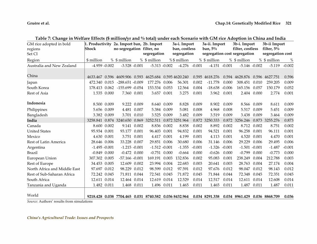
Gruère et al. Chap.14: Genetically Modified Rice 321
China's Agricultural Trade: Issues and Prospects
Table 7: Change in Welfare Effects ($ million/yr and % total) under each Scenario with GM rice Adoption in China and India
GM rice adopted in bold regions Set CI
1. Productivity Shock
2a. Import ban, no segregation
2b. Import filter, no segregation
3a-i. Import ban, costless segregation
3a-ii. Import ban, 5% segregation cost
3b-i. Import filter, costless segregation
3b-ii Import filter, 5% segregation cost
Region $ million % $ million % $ million % $ million % $ million % $ million % $ million %
Australia and New Zealand -4.959 -0.002 -3.528 -0.001 -5.313 -0.002 -4.276 -0.001 -4.151 -0.001 -5.146 -0.002 -5.119 -0.002
China 4633.467 0.596 4609.906 0.593 4625.684 0.595 4620.240 0.595 4618.276 0.594 4628.876 0.596 4627.751 0.596
Japan 472.340 0.015 -288.651 -0.009 177.276 0.006 56.301 0.002 -11.778 0.000 308.451 0.010 259.205 0.009
South Korea 178.413 0.062 -155.699 -0.054 153.534 0.053 12.564 0.004 -18.638 -0.006 165.156 0.057 150.179 0.052
Rest of Asia 1.535 0.000 7.360 0.001 3.657 0.001 3.275 0.001 3.962 0.001 2.404 0.000 2.774 0.001
Indonesia 8.500 0.009 9.222 0.009 8.640 0.009 8.828 0.009 8.902 0.009 8.566 0.009 8.611 0.009
Philippines 5.656 0.009 4.481 0.007 5.384 0.009 5.081 0.008 4.968 0.008 5.517 0.009 5.451 0.009
Bangladesh 3.382 0.009 3.701 0.010 3.525 0.009 3.482 0.009 3.519 0.009 3.438 0.009 3.464 0.009
India 3258.841 0.874 3240.650 0.869 3252.511 0.872 3251.964 0.872 3250.333 0.872 3256.246 0.873 3255.276 0.873
Canada 8.600 0.002 9.141 0.002 8.836 0.002 8.838 0.002 8.892 0.002 8.712 0.002 8.751 0.002
United States 95.934 0.001 93.177 0.001 96.403 0.001 94.832 0.001 94.521 0.001 96.258 0.001 96.111 0.001
Mexico 4.630 0.001 3.751 0.001 4.417 0.001 4.199 0.001 4.113 0.001 4.520 0.001 4.470 0.001
Rest of Latin America 28.646 0.006 33.228 0.007 29.851 0.006 30.680 0.006 31.146 0.006 29.229 0.006 29.495 0.006
Argentina -1.495 -0.001 -1.215 -0.001 -1.512 -0.001 -1.355 -0.001 -1.326 -0.001 -1.501 -0.001 -1.487 -0.001
Brazil -0.849 0.000 -0.472 0.000 -0.751 0.000 -0.664 0.000 -0.626 0.000 -0.799 0.000 -0.773 0.000
European Union 307.302 0.005 -57.166 -0.001 169.191 0.003 132.836 0.002 95.083 0.001 238.249 0.004 212.788 0.003
Rest of Europe 34.453 0.005 12.609 0.002 23.994 0.004 22.683 0.003 20.641 0.003 28.763 0.004 27.174 0.004
North Africa and Middle East 97.697 0.012 98.229 0.012 98.599 0.012 97.591 0.012 97.676 0.012 98.047 0.012 98.143 0.012
Rest of Sub-Saharan Africa 72.242 0.045 71.811 0.044 72.541 0.045 71.872 0.045 71.844 0.044 72.348 0.045 72.351 0.045
South Africa 12.611 0.014 12.464 0.014 12.619 0.014 12.529 0.014 12.517 0.014 12.611 0.014 12.608 0.014
Tanzania and Uganda 1.482 0.011 1.468 0.011 1.496 0.011 1.465 0.011 1.465 0.011 1.487 0.011 1.487 0.011
World 9218.428 0.038 7704.465 0.031 8740.582 0.036 8432.964 0.034 8291.338 0.034 8961.429 0.036 8868.709 0.036 Source: Authors‘ results from simulations

Gruère et al. Chap.14: Genetically Modified Rice 322
China's Agricultural Trade: Issues and Prospects
rice. Therefore, in most cases, sensitive countries gain overall from the adoption of GM
rice.
Discussion
The results of our international economy-wide simulations vary across regions and
scenarios, but they share a number of similarities, that can help us draw a few general
lessons. First, our simulations show that the adoption of GM rice by India and/or China
would result in significant economic gains in these countries and globally in the
presence or absence of trade restrictions in certain sensitive countries. Only a few
regions experience net losses with the adoption of GM rice, and these losses are
relatively insignificant, except perhaps in sensitive countries with trade bans or when
segregation results in a 5% additional trade cost for their non-GM rice imports.
However, these developed countries have adopted restrictive policies in the presence of
positive consumer willingness to pay to avoid GM food products, so these relatively
small real income losses might not be actual welfare losses. At the same time, under our
assumptions, the model shows that adopting GM rice in China and India results in
significant economic gains, based on technical efficiency gains, and associated with large
increases in rice production and large reduction of imports.
Table 8: Relative Effects of Trade Restriction on Total Gains from GM Rice Adoption for Selected Countries in the Three Sets of Scenarios
Set C I CI
Scenarios 1 vs. 2a 1 vs. 2b 1 vs. 2a 1 vs. 2b 1 vs. 2a 1 vs. 2b
China 0.51% 0.17% 0.51% 0.17% India 0.59% 0.21% 0.56% 0.19% World 23% 7.0% 5.9% 2.3% 16.4% 5.2% Source: Simulation results
Secondly, our simulations show that trade regulations would affect the gains from
GM rice adoption, but that this effect is insignificant compared to the gains with the
adoption of GM rice. A complete import ban of rice from GM producing countries in
sensitive countries results in lower gains for an exporter like India. Similarly, applying a
trade filter that allows only products for intermediate consumption to enter sensitive
countries, reflecting the effects of current labeling regulations on GM food, slightly
reduces the gains of exporting GM adopting countries. Yet, even with these barriers,
China or India would largely gain from the adoption of GM rice, because their relative

Gruère et al. Chap.14: Genetically Modified Rice 323
China's Agricultural Trade: Issues and Prospects
loss with trade restrictions is very small compared to the productivity gains they
experience domestically. To emphasize this result, Table 8 shows the relative change in
gains from GM rice under the most restrictive scenarios of each set. Even if globally, the
gains are reduced by up to 23% overall (in the first set), we find that the reduction in
gains for India or China is less or equal to 0.6% of the overall gains they obtain with GM
rice. This means that for each 100 dollars of real income gains with GM rice, China or
India would risk losing 60 cents due to the possible ban in import-sensitive countries.
Table 9: Opportunity Cost of Segregation of non-GM Rice for Adopting and
Sensitive Countries ($ million/year)
$million/year Country Segregation of non-GM rice for final consumption only
Segregation of non-GM rice for final and intermediate
consumption
SET C I CI C I CI
China 3.1 0.1 2.9 9.8 0.2 10.3
India -0.1 3.7 3.7 -0.3 10.9 11.3
Total GM producers 3.1 3.7 6.6 9.8 10.9 21.6
Australia-NZ -0.1 0.3 0.2 -1 0.3 -0.8
Japan 126.1 5.0 131.2 330 14 345
South Korea 11.3 0.4 11.6 162.2 4.3 168.3
EU 32.6 34.2 69.1 90.3 86.5 190
Rest of Europe 3.6 1.1 4.8 7.4 2.5 10
Total sensitive countries 173.5 41 216.9 588.9 107.6 712.5
Global 175.3 43.3 220.9 597.8 114.5 728.5 Source: Authors‘ derivations
Thirdly, the use of segregation for non-GM crops can help offset some of these
relatively minor losses for GM rice adopters, even at a 5% costs. Estimates of the
opportunity costs of segregation are reported for selected countries in Table 9. We can
draw several conclusions from these derivations. First, these results show that GM
producing countries have a positive but relatively limited opportunity cost of
segregation, ranging from $3 to 4million/year for final rice product to about $7 million
per year for rice going towards intermediate consumption. Second, segregation would
be as valuable for China as for India, even if segregation would be globally much more
valuable when China adopts than when India adopts GM rice. Third, we find that
segregation of non-GM rice for intermediate consumption would matter more than
segregation of non-GM rice for final consumption.

Gruère et al. Chap.14: Genetically Modified Rice 324
China's Agricultural Trade: Issues and Prospects
More generally, we find that most of the global benefits of segregation would occur
in importing sensitive countries themselves. For instance, when the two countries adopt
GM rice, segregating non-GM rice for final consumption results in global gains of $221
million per year, of which $217 million would occur in sensitive countries and only $6.6
million in China and India. Similarly, under the same set, the segregation of non-GM
rice for final and intermediate consumption results in increased gains of about $728m
per year, of which $712 million would go to sensitive countries and only $21 million to
GM rice adopters. Consequently, these results suggest that the adoption of GM rice in
India or China may not necessarily require high investment by traders willing to keep
their market in sensitive countries. Because the immediate cost of bans will largely be
borne by importers, they will have a clear incentive to invest in segregation or at least to
make sure GM rice is approved and the import bans are replaced by trade filters.
Fourth, we find that India and China can act independently on GM rice, because
they do not share competing interests. The gains to China remain the same if India
adopts GM rice or if it does not, despite the relative price decline with both countries
adopting. Similarly, the gains to India remain the same, whether China adopts or not.
But the order of leadership makes a small difference. If China leads the world by
adopting GM rice, India would incur very small losses in rice export, and suffer a small
and relatively insignificant decline in real income if it does not follow China. On the
other hand, if India adopts GM rice first, China would actually gain a small and
relatively insignificant welfare amount, even if it slightly reduces its exports of rice. We
would expect the same type of effect with other net exporting or small exporting and
importing countries: large exporters will loss from a rival adopting a productivity
enhancing technology, while small exporters and importers will not necessarily lose and
may even gain from it.
Overall, we obtain larger gains for GM rice in India or globally than previous studies.
For China, our results can be compared to the ones of Huang et al. (2004). Our slightly
larger results likely come from the fact that unlike Huang et al. (2004), we do not
explicitly reduce the gains from GM crops due to the price of seeds. Therefore the gains
presented here include the returns to the developers and adopting producers together.
For India, our results are much larger than the ones in other studies. The difference may
come from the selected productivity shock, the adoption rate, or the scenarios. Because

Gruère et al. Chap.14: Genetically Modified Rice 325
China's Agricultural Trade: Issues and Prospects
we impose factor-biased productivity shocks with large efficiency gains in certain critical
sectors, our results may be different from the imposition of a Hicks-neutral 5% shock
with GM rice. Moreover, as we combine the effects of different traits, the total effect of
GM rice in our model is quite large compared to only Bt rice or drought resistant rice.
Hareau et al. (2005) also differentiate traits but they do not impose a shock on the
chemical or labor factor for Bt rice.
Despite the differences with previous studies, we believe that our results are likely
to be robust for India, in particular because they rely on primary and secondary data on
productivity potential rather than generalized parameters. Still, like any ex-ante
simulation exercise, the results depend on the assumptions of the model and scenarios.
One of the critical factors is the yield effect. To verify the validity of the results we ran
four sets of additional simulations (for scenarios 1, 2a, 3a-i and 3a-ii) using the minimum
and maximum values for yields in India presented in Table 2. The results are shown in
Table A6 in the Appendix. As expected, the welfare effects are consistently lower for
India with the minimum yield effects than with the most likely yield effects. The welfare
effects are also consistently larger for India with maximum yield gains, which means
that the price decline with this higher rice production is still compensated by larger
gains for India overall. At the same time, the relative differences across scenarios are
proportionally similar to the ones with most likely gains. India gains most under
scenario 1 and least under scenario 2a, and segregation of non-GM rice compensates for
the small reduction in gains with rice trade bans.
Table 10: Welfare Gains per percent Actual Adoption of GM Rice in each Scenario ($ million)
SET Country 1 2a 2b 3a-i 3a-ii 3b-i 3b-ii
C China 57.9 57.6 57.8 57.7 57.7 57.8 57.8
I India 45.5 45.2 45.4 45.4 45.3 45.4 45.4
CI China 57.9 57.6 57.8 57.8 57.7 57.9 57.8
India 45.4 45.2 45.3 45.3 45.3 45.4 45.4 Source: Authors‘ derivations
A second critical factor is the adoption rate. To provide a consistent idea of the
welfare gains experienced by the countries in our study, we divided the total annual real
income gains by the final adoption rates (presented in Table 3). The results are shown in

Gruère et al. Chap.14: Genetically Modified Rice 326
China's Agricultural Trade: Issues and Prospects
million dollars per year per percentage of adoption in Table 10. We find that the gains
are fairly homogeneous across scenarios. China gains just under $58 million for each
percentage point of Bt rice in total rice production, while India gains above $45 million
for each percentage point of the GM rice with our combination of traits. The difference
between the two countries is mainly due to the total value of rice production and in the
assumptions we made in the two countries. In any case, these result show that GM rice
would be largely beneficial even at a lower adoption rate.
Conclusions
Many developing countries have delayed the adoption of GM crops for fear of losing
export markets in the EU and other countries with stringent regulations on the approval
and marketing of GM food. Yet, previous trade studies have shown that despite the
presence of these importing countries´ regulations, the production of relevant GM crops
in developing countries is still expected to provide significant net welfare gains
(Anderson and Jackson, 2005).
In this paper we study the potential effects of introducing GM rice in India with or
without China. We focus on four types of GM rice resistant to biotic and abiotic stresses,
such as drought resistant rice and use a multi-country, CGE model to simulate their
introduction in India. We build on previous international simulation models by
improving the representation of the productivity shocks with GM rice taking into
account regional and land type disparities and by using an updated representation of
the world market, accounting for the short run and long run effects of import approval
and labeling policies in sensitive countries. We also allow for the possibility of
segregation for non-GM rice products going towards sensitive importing countries.
First, the results of our simulations show that the gains associated with the partial
adoption of our combination of traits for GM rice in India are quite significant,
accounting for about 0.9% of total real income or over $3.2 billion annually. Our results
show that a 1% increase in the adoption of GM rice in India, combining different traits in
different regions, would result in total welfare gains exceeding $45 million per year,
with or without trade blocks in sensitive countries. Similarly, using the assumptions
made by Huang et al. (2004), we find that a 1% increase in Bt rice in China would result
in gains exceeding $57 million per year.

Gruère et al. Chap.14: Genetically Modified Rice 327
China's Agricultural Trade: Issues and Prospects
Second, we find that these results largely exceed any type of potential trade losses
for India. In India like in China, with GM rice, even at partial adoption rates, the losses
with trade restrictions does not exceed 0.6% of the total gains with GM rice adoption.
Provided it is adopted, GM rice would also result in large production increases, which
could result in relative welfare gains in countries of Sub-Saharan Africa or rice
importing countries of Asia. At the same time, we find that segregation can help reduce
a significant share of the potential welfare gain reductions due to trade losses for GM
rice adopters that want to keep export opportunities in sensitive countries. Our results
also show that the opportunity cost of segregation for non-GM rice is much larger for
sensitive importing countries than exporting countries adopting GM rice. This suggests
that importers will likely have the incentive to invest into segregation chains for non-
GM supplies to mitigate their expected losses due to the introduction of GM crops in
exporting countries.
Therefore, our results demonstrate that some of the perceived trade losses related to
the use of GM rice, a major food crop in Asia are exaggerated in the current market
situation. It is certain that trade barriers could multiply with the adoption of trade
distorting regulations in a larger set of countries. For instance, India is exporting more
rice towards North African and the Middle East than towards Europe, and some of these
countries could decide to enforce strict import policies. But a large share of the economic
losses with these possible restrictions would likely incur in these particular countries.
Still, in the current regulatory environment, where enforced regulations are
concentrated in a few importers, India and China are bound to largely gain from
adopting GM rice. Because India and China have very large population bases with high
consumption rates, any increase in rice productivity will most likely overcome any
potential trade losses.
Third, we find that there is no significant first mover-advantage for GM rice in India
and China even if India would be slightly better off leading than following on the
adoption of GM rice. China and India would gain as much by adopting GM rice if the
other adopts it than if it does not. At the same time, India might incur small losses if
China adopts GM rice at a significant level, because of its potential loss in
competitiveness, while China would not lose and would potentially gain a little if it
waited for India to be first. If we consider our assumptions to be relatively conservative

Gruère et al. Chap.14: Genetically Modified Rice 328
China's Agricultural Trade: Issues and Prospects
(e.g., with weighted average of yield effects from different data sources), it is possible
that India would be better off leading in technology adoption, but our results are not
sufficient to warrant that conclusion. Still, our main conclusion is that China and India
would largely gain from GM rice adoption, even when faced with trade restrictions in
sensitive countries. China faces even less potential economic risk than India, and should
be encouraged to move ahead, given its technology edge in GM rice. Such a move would
clearly encourage India to follow, provided GM rice can be approved by its biosafety
authorities.
Even if our simulations are based on improvements in assumptions and scenarios,
they are still subject to a number of limitations. First, like in any ex-ante simulation, the
productivity effects are still largely uncertain and their level affects the results
significantly. A sensitivity analysis on the yield factors showed that larger yield gains
result in higher welfare gains, but that the losses with trade remain relatively small
compared to the gains with GM technology. More sensitivity analysis, particularly on
the input factors would help to provide a more complete picture of the range of possible
effects of GM rice in India. Second, our simulation would gain by using a dynamic
rather than comparative static framework. Local expert meetings and elicitation
provided some insight into the potential evolution of adoption in India. Accounting for
the crop/trait specific regulatory lag, extension lags and adoption dynamics would help
improve the plausibility of our results and allow us to introduce more strategic
considerations. If not, the use of a more recent representation of the economy would at
least provide a better overview of the situation. Third, despite our effort to reduce
potential biases linked to the over-aggregation of the GTAP database with the use of
proportional factors for agricultural chemical, our model would be better served with
structural differentiation within the chemical sector.
More generally, it is necessary to keep in mind that the results of our global
simulations, like the ones of other papers, do not account for the positive or negative
effects of technology adoption on the environment and other potential externalities they
may generate on other activities of the economy. On the one hand, the reduction of
chemical inputs may provide benefit for farmers‘ health and/or the environment, on the
other hand, secondary or non-target pest resistance building may affect other types of
crop production and potential gene flows could affect natural biodiversity. Our implicit

Gruère et al. Chap.14: Genetically Modified Rice 329
China's Agricultural Trade: Issues and Prospects
assumption throughout the chapter is that the varieties of GM rice we consider are only
released after assessment and approval by the biosafety regulatory authorities in India
and China, on the conclusion that their potential risks are negligible or at least
manageable under particular practices. Naturally any possible external costs incurred in
adopting countries would have to be compared with the large expected income gains we
found in these two countries.
References
Anderson, K. and L.A. Jackson. ―Some Implications of GM Food Technology Policies for Sub-Saharan Africa,‖ Journal of African Economies 14 (2005): 385-410.
Anderson, K., L.A. Jackson, and C.P. Nielsen. ―Genetically Modified Rice Adoption: Implications for Welfare and Poverty Alleviation,‖ World Bank Policy Research Working Paper No. 3380. Washington, DC: World Bank (2004)
Anderson, K. and S. Yao. ―China, GMOs and World Trade in Agricultural and Textile Products,‖ Pacific Economic Review 8 (2003): 157-69.
Annou, M.M, F.H. Fuller, and E.J. Wailes. ―Innovation Dissemination and the Market Impacts of Drought-Tolerant, Genetically Modified Rice,‖ International Journal of Biotechnology 7(2005):113-127.
Bchir, M.H., Y.Decreux, J-L. Guerin, and S. Jean. ―MIRAGE, a Computable General Equilibrium for Trade Policy Analysis,‖ Working Paper No. 2002-17. Paris: Centre d‘Etudes Prospectives et d‘Informations Internationales (2002).
Bennett, R.M., Y. Ismael, U. Kambhampati, and S. Morse. ―Economic Impact of Genetically Modified Cotton in India,‖ AgBioForum 7 (2004): 96-100.
Berwald, D., C.A. Carter, and G.P. Gruere. ―Rejecting New Technology: The Case of Genetically Modified Wheat,‖ American Journal of Agricultural Economics 88 (2006):432-447.
Elbehri, A. and S. MacDonald. ―Estimating the Impact of Transgenic Bt Cotton on West and Central Africa: A General Equilibrium Approach,‖ World Development 32 (2004): 2049-64.
Evenson, R.E., R.W. Herdt, and M. Hossain. Rice Research in Asia: Progress and Priorities. Wallington: CAB International (1996).
Fischer, G., H. van Velthuizen, M. Shah, and F. Nachtergaele. ―Global Agro-ecological Assessment for Agriculture in the 21st Century: Methodology and Results,‖ No. RR-02-02. Laxenburg: Institute for Applied Systems Analysis (2002).
Gruere, G.P. ―An Analysis of Trade Related International Regulations of Genetically Modified Food and their Effects on Developing Countries,‖ EPTD Discussion Paper No. 147. Washington, DC: International Food Policy Research Institute (2006).
Gruere, G.P. and S.R. Rao. ―A Review of International Labeling Policies to Evaluate India's Proposed Rules,‖ AgBioForum 10 (2007): 51-64.
Hareau, G., G.W. Norton, B.F. Mills, and E. Peterson. ―Potential Benefits of Transgenic Rice in Asia: A General Equilibrium Analysis,‖ Quarterly Journal of International Agriculture 44 (2005): 205-21.

Gruère et al. Chap.14: Genetically Modified Rice 330
China's Agricultural Trade: Issues and Prospects
Huang, J., R. Hu, H. van Meijl, and F. van Tongeren. ―Biotechnology Boosts to Crop Productivity in China: Trade and Welfare Implications,‖ Journal of Development Economics 75 (2005): 27-54.
Hertel, T. W. (ed). Global Trade Analysis: Modeling and Applications. New York: Cambridge University Press (1997).
International Food Policy Research Institute. ―An Economic Analysis of Domestic and International Biosafety and Marketing Regulations for Agricultural Biotechnology in India and Bangladesh,‖ Unpublished Donor Report. Washington, DC: International Food Policy Research Institute (April September 2005).
James, C. ISAAA. ―Global Status of Commercialized Biotech/GM Crops: 2006,‖ ISAAA Brief No. 35-2006 (2006).
Paarlberg, R.L. ―The Real Threat to GM Crops in Poor Countries: Consumer and Policy Resistance in Rich Countries,‖ Food Policy 27 (2002): 247-50.
Pray, C., J. Huang, R. Hu, and S. Rozelle. ―Five Years of Bt Cotton in China - The Benefits Continue,‖ The Plant Journal 31 (2002): 423-30.
Runge, C.F. and B. Ryan. ―The Global Diffusion of Plant Biotechnology: International Adoption and Research in 2004,‖ Minneapolis-St.Paul, MN: University of Minnesota, Center for International Food and Agricultural Policy (2004).
Sánchez, P.A, W. Couto, and S.W. Buol. ―The Fertility Capability Soil Classification System: Interpretation, Applicability and Modification,‖ Geoderma 27 (1982): 283–309.
Smale, M., P. Zambrano, J. Falck-Zepeda, and G. Gruere. ―Parables: Applied Economics Literature about the Impacts of Genetically Engineered Varieties in Developing Economies,‖ EPTD Discussion Paper No. 158. Washington, DC: International Food Policy Research Institute (October 2006).
Smith, C., R. Yost, J. Benites, and F. Nachtergaele. ―Fertility Capability Classification (FCC) System - 3rd Approximation: The Algorithm and an Application.‖ Paper No. 862 in 16th World Congress of Soil Science, A. Ruellan (ed.). Montpellier: International Society of Soil Science (1988).
You, L. and S. Wood. ―An Entropy Approach to Spatial Disaggregation of Agricultural Production,‖ Agricultural Systems 90 (2006): 329-347.
Yudelman, M., A. Ratta, and D. Nygaard. ―Pest Management and Food Production: Looking to the Future,‖ 2020 Food Agriculture and the Environment Discussion Paper No. 25. Washington, DC: International Food Policy Research Institute (1998).

Gruère et al. Chap.14: Genetically Modified Rice 331
China's Agricultural Trade: Issues and Prospects
Appendix: Additional Tables
Table A1: Decomposition of the Welfare Gains for Scenario 1 under each Set (% of total real income)
SET Country Real income Allocation efficiency
gains
Terms of trade gains
Other gains
C China 0.60 0.04 0.03 0.53
India 0.00 0.00 0.00 0.00
I China 0.00 0.00 0.00 0.00
India 0.88 0.14 -0.01 0.74
CI China 0.60 0.04 0.03 0.53
India 0.87 0.14 -0.01 0.75 Source: Results from simulations
Table A2: % Change in Average World Price of Rice Under Different Scenarios
Scenario China India India + China
1 -0.634 -0.826 -1.502
2a -0.383 -0.665 -1.067
2b -0.587 -0.797 -1.423
3a-i -0.568 -0.811 -1.419
3a-ii -0.520 -0.764 -1.348
3b-i -0.634 -0.831 -1.504
3b-ii -0.597 -0.792 -1.453
Source: Results from simulations.
Table A3: % Changes in Production, Export and Import Volumes of Rice for Set C Scenarios in Selected Countries
Country % change in 1 2a 2b 3a-i 3a-ii 3b-i 3b-ii
China Production 20.1 18.2 19.9 18.9 18.8 19.9 19.9
Exports 27.3 -11.7 13.7 56.7 41.0 36.9 23.6
Imports -46.9 -47.6 -47.1 -47.3 -47.3 -47.0 -47.1
India Production -0.4 0.0 -0.4 -0.2 -0.6 -0.4 -0.8
Exports -5.7 -1.9 -4.7 -3.6 -7.7 -5.1 -9.0
Imports -1.3 -1.9 -1.3 -1.6 -1.9 -1.3 -1.5
Japan Production -2.1 1.8 -1.5 0.0 0.4 -1.7 -1.5
Exports -2.8 -4.2 -3.0 -3.6 -3.7 -2.9 -2.9
Imports -4.2 0.7 -2.9 11.7 8.8 1.4 -1.5
EU Production -6.8 5.4 -5.9 0.0 2.6 -6.3 -4.5
Exports -5.0 -5.5 -3.7 -5.5 -5.9 -4.3 -4.6
Imports -7.1 3.8 -4.8 8.2 3.8 -2.7 -7.4
Rest of Asia Production -1.7 -1.1 -1.6 -1.4 -1.3 -1.6 -1.6
Exports -8.5 -6.4 -7.8 -7.4 -7.0 -8.1 -7.8
Imports -1.9 -3.2 -2.1 -2.7 -2.7 -2.0 -2.0 Source: Results from simulations

Gruère et al. Chap.14: Genetically Modified Rice 332
China's Agricultural Trade: Issues and Prospects
Table A4: % Changes in Production, Export and Import Volumes of Rice for Set I Scenarios in Selected Countries
Country % change in 1 2a 2b 3a-i 3a-ii 3b-i 3b-ii
China Production -0.1 0.0 -0.1 -0.1 -0.3 -0.1 -0.3
Exports -5.8 -4.9 -4.9 -4.3 -11.3 -5.4 -12.3
Imports 1.0 0.9 1.0 0.9 0.8 1.0 0.8
India Production 21.0 17.0 20.8 19.0 18.6 20.9 20.7
Exports 26.1 17.7 17.7 39.3 31.3 30.5 23.1
Imports -50.7 -50.9 -50.9 -50.9 -51.0 -50.8 -50.8
Japan Production -0.3 -0.1 -0.2 -0.2 0.2 -0.2 0.2
Exports -2.5 -2.4 -2.4 -2.3 -2.5 -2.4 -2.6
Imports 0.4 0.9 0.3 0.9 -2.1 0.6 -2.4
EU Production -7.1 6.5 -6.1 -1.2 1.6 -6.6 -4.6
Exports -5.8 -5.6 -5.6 -7.3 -7.7 -5.7 -6.0
Imports -4.7 11.8 -5.0 11.8 7.0 0.1 -5.1
Rest of Asia Production -1.2 -0.9 -1.2 -1.1 -1.0 -1.2 -1.1
Exports -7.3 -6.8 -6.8 -6.5 -6.1 -7.0 -6.7
Imports -1.6 -1.5 -1.5 -1.5 -1.6 -1.6 -1.7 Source: Results from simulations
Table A5: % Changes in Production, Export and Import Volumes of Rice for Set CI Scenarios in Selected Countries
Country % change in 1 2a 2b 3a-i 3a-ii 3b-i 3b-ii
China Production 19.8 18.0 19.6 18.8 18.6 19.7 19.6
Exports 20.6 7.6 7.6 51.4 35.8 30.5 17.6
Imports -46.4 -46.6 -46.6 -46.8 -46.9 -46.5 -46.6
India Production 20.2 16.6 20.0 18.7 18.2 20.1 19.9
Exports 19.7 12.1 12.1 35.4 27.3 24.7 17.6
Imports -51.3 -51.5 -51.5 -51.7 -51.8 -51.4 -51.4
Japan Production -2.3 1.7 -1.7 -0.1 0.2 -2.0 -1.7
Exports -5.1 -5.1 -5.1 -5.7 -5.8 -5.1 -5.2
Imports -3.7 -2.5 -2.5 12.7 9.8 2.1 -0.8
EU Production -12.7 13.3 -10.9 -1.2 1.5 -11.9 -10.5
Exports -10.4 -8.8 -8.8 -12.0 -12.3 -9.6 -9.8
Imports -9.8 -8.9 -8.9 21.9 16.8 -0.7 -6.1
Rest of Asia Production -2.8 -1.8 -2.7 -2.4 -2.3 -2.7 -2.7
Exports -15.1 -14.0 -14.0 -13.4 -13.0 -14.6 -14.3
Imports -3.3 -3.4 -3.4 -4.0 -4.1 -3.4 -3.4 Source: Results from simulations

Gruère et al. Chap.14: Genetically Modified Rice 333
China's Agricultural Trade: Issues and Prospects
Table A6: Change in Welfare Effects with GM Rice Adoption in India and China, under Minimum, Most Likely and Maximum Yield Effects for India in the Case of Selected Scenarios ($ million/year)
Set CI 1. Productivity shock 2a. Import ban, no segregation 3a-i. Import ban, costless
segregation 3a-ii. Import ban, 5%
segregation cost
Region Minimum Most likely Maximum Minimum
Most likely Maximum Minimum
Most likely Maximum Minimum
Most likely Maximum
Australia and NZ -4.624 -4.959 -5.280 -3.082 -3.528 -3.963 -3.903 -4.276 -4.616 -3.763 -4.151 -4.512
China 4633.076 4633.467 4633.918 4609.292 4609.906 4610.572 4619.637 4620.24
0 4620.903 4617.649 4618.276 4618.966
Japan 462.008 472.340 483.624 -294.727 -288.651 -282.297 46.955 56.301 67.048 -20.450 -11.778 -1.929
South Korea 175.953 178.413 181.170 -157.071 -155.699 -154.217 10.187 12.564 15.419 -20.836 -18.638 -16.022
Rest of Asia 5.346 1.535 -1.509 10.523 7.360 4.956 7.138 3.275 0.023 7.730 3.962 0.816
Indonesia 6.677 8.500 10.354 7.343 9.222 11.138 6.997 8.828 10.679 7.063 8.902 10.763
Philippines 5.079 5.656 6.255 3.936 4.481 5.045 4.503 5.081 5.685 4.395 4.968 5.567
Bangladesh 2.407 3.382 4.436 2.656 3.701 4.826 2.500 3.482 4.527 2.527 3.519 4.576
India 2287.077 3258.841 4200.295 2272.197 3240.650 4178.408 2280.720 3251.96
4 4193.407 2279.559 3250.333 4191.185
Canada 7.820 8.600 9.453 8.328 9.141 10.027 8.058 8.838 9.683 8.107 8.892 9.742
United States 87.591 95.934 104.467 85.323 93.177 101.220 86.563 94.832 103.374 86.324 94.521 102.980
Mexico 4.193 4.630 5.119 3.343 3.751 4.209 3.764 4.199 4.690 3.683 4.113 4.600
Rest of L. America 28.715 28.646 28.593 33.126 33.228 33.346 30.782 30.680 30.548 31.224 31.146 31.042
Argentina -1.020 -1.495 -1.986 -0.745 -1.215 -1.701 -0.880 -1.355 -1.847 -0.851 -1.326 -1.817
Brazil -0.629 -0.849 -1.076 -0.282 -0.472 -0.668 -0.449 -0.664 -0.892 -0.415 -0.626 -0.848
European Union 273.696 307.302 343.115 -69.058 -57.166 -44.103 100.990 132.836 171.042 66.467 95.083 129.370
Rest of Europe 32.081 34.453 37.138 11.009 12.609 14.473 20.478 22.683 25.334 18.552 20.641 23.144
N. Africa and M. East 76.043 97.697 119.926 76.151 98.229 120.912 75.875 97.591 119.797 75.901 97.676 119.954
Rest of S-S Africa 63.554 72.242 81.054 62.989 71.811 80.781 63.157 71.872 80.690 63.112 71.844 80.686
South Africa 9.115 12.611 16.037 8.944 12.464 15.916 9.026 12.529 15.955 9.011 12.517 15.948
Tanzania and Uganda 1.166 1.482 1.805 1.143 1.468 1.801 1.147 1.465 1.788 1.146 1.465 1.789
World 8155.321 9218.428 10256.905 6671.335 7704.465 8710.683 7373.246 8432.96
4 9473.238 7236.13
4 8291.338 9325.999 Source: Results from simulations