Open Journal of Civil Engineering, 2015, 5, 289-298 Published Online September 2015 in SciRes. http://www.scirp.org/journal/ojce http://dx.doi.org/10.4236/ojce.2015.53029

How to cite this paper: Aidara, M.L.C., Ba, M. and Carter, A. (2015) Choice of an Advanced Rheological Model for Modeling the Viscoelastic Behavior of Hot Mixtures Asphalt (HMA) from Sénégal (West Africa). Open Journal of Civil Engineering, 5, 289-298. http://dx.doi.org/10.4236/ojce.2015.53029

Choice of an Advanced Rheological Model for Modeling the Viscoelastic Behavior of Hot Mixtures Asphalt (HMA) from Sénégal (West Africa) Mouhamed Lamine Chérif Aidara1, Makhaly Ba1, Alan Carter2 1UFR Engineering sciences, Thiès University, Thiès, Sénégal 2School of Superior Technologies (ETS), Director of Pavement Bituminous Materials Laboratory (LCMB), Montreal, Canada Email: mouhamedlamine.aidara@univ-thies.sn Received 3 July 2015; accepted 25 August 2015; published 28 August 2015

Copyright © 2015 by authors and Scientific Research Publishing Inc. This work is licensed under the Creative Commons Attribution International License (CC BY). http://creativecommons.org/licenses/by/4.0/

Abstract The main purpose of this article is to choose among advanced rheological models used in the French rational design, one that best represents the viscoelastic behavior of asphalt mixtures mixed with aggregates of Senegal. The model chosen will be the basis for the development of computational tools for stress and strain for Senegal. However, the calibration of these models needs complex modulus test results. In opposition to mechanical models the complex modulus can directly characterize the viscoelastic behavior of bituminous materials. Here determination is performed in the laboratory by using several types of tests divided into two groups: homogeneous tests and non-homogeneous tests. The choice of model will be carried out by statistical analysis through the least squares method. To this end, a study was carried out to “Laboratory of Pavement and Bituminous Materials” (LCMB) with asphalt concrete mixed with aggregate from Senegal named basalt of Diack and quartzite of Bakel. In this study, the test used to measure the complex modulus is the Canadian test method LC 26-700 (Determination of the complex modulus by ten-sion-compression). There mainly exist two viewing complex modulus planes for laboratory test results: the Cole and Cole plane and the Black space. The uniqueness of the data points in these two areas means that studied asphalt concretes are thermorheologically simple and that the prin-ciple of time-temperature superposition can be applied. This means that the master curve may be drawn and that the same modulus value can be obtained for different pairs (frequency- tempera-ture). These master curves are fitted during the calibration process by the advanced rheological models. One of the most used software in the French rational design for the visualization of com-plex modulus test results and calibration of rheological models developed tools is named Vis-co-analysis. In this study, its use in interpreting the complex modulus test results and calibration

M. L. C. Aidara et al.

290

models shows that, the studied asphalt concretes are thermorheologically simple, because they present good uniqueness of their Black and Cole and Cole and Black diagrams. They allow a good application of the principle of time temperature superposition. The statistical analysis of calibra-tion models by the least squares method has shown that the three studied models are suitable for modeling the linear viscoelastic behavior of asphalt mixtures formulated with the basalt of Diack and the quartzite of Bakel. Indeed their calibration has very similar precision values of “Sum of Squared Deviation” (SSD) about 0.185. However, the lower precision value (0.169) is obtained with the 2S2P1D model.

Keywords Complex and Dynamic Modulus, Viscoelastic, Huet, Huet-Sayegh, 2S2D1P, Visco-Analyse, Sum of Squared Deviation

1. Introduction Asphalt concretes behavior is linear viscoelastic to low deformations and low cycles of loading [1]. This beha-vior is intermediate between the behavior of a perfect elastic solid and that of a Newtonian liquid [2]. In a linear viscoelastic behavior, the material properties are assumed independents of the applied stress or strain levels. The analysis of the linear viscoelastic behavior is done either by using the rheological models, or complex modulus, or creep compliance. These three methods are linked. In fact the conversion from creep compliance to the me-chanical model is possible by the method of successive residuals, and the change from the complex modulus to creep compliance by the Fourier transforms [2]. The complex modulus E* is defined as a complex number that links stress to strain for a linear viscoelastic material subjected to a sinusoidal loading [3]. The absolute value of the complex modulus is commonly referred to as the “dynamic” modulus |E*| [4]. The phase angle φ characte-rizes the deviation between stress and strain of a viscoelastic material. The |E*| is an approximation of the elastic modulus of a viscoelastic material, which can be used for pavement design when the laws of elasticity are em-ployed. When the laws of viscoelasticity are applied, the mechanical models are used. In pavement design, the asphalt concrete layer can be considered as elastic or viscoelastic materials. The MEPDG [5] and the Alizé- LCPC software’s [6] consider asphalt concretes as elastic materials, characterized by dynamic modulus and Poisson ratio. Software which uses viscoelastic behavior needs to calibrate viscoelastic analogic model like the Huet, the Huet-Sayegh and the 2S2P1D models by complex modulus laboratory test results. In this study these models will be calibrated with results from complex modulus test (LC 26-700) performed with six asphalt con-cretes. The goodness of fit is measured statistically by the least squares method through the “Sum of Squared Deviation” (SSD).

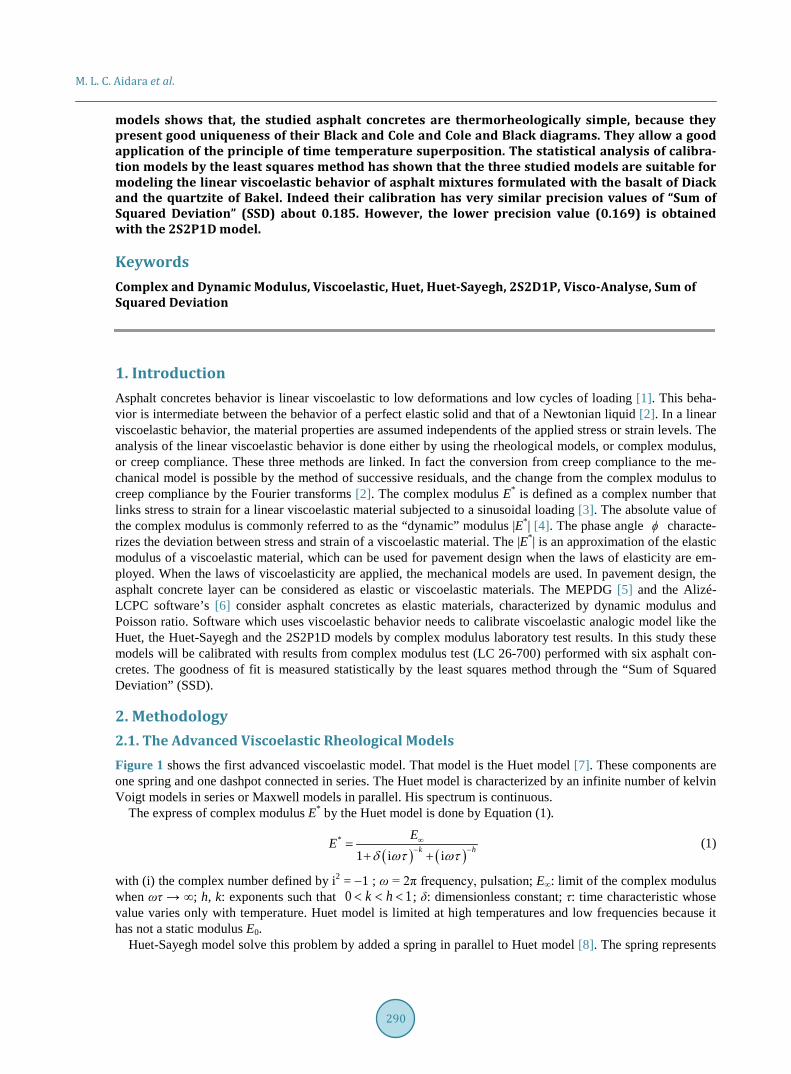
2. Methodology 2.1. The Advanced Viscoelastic Rheological Models Figure 1 shows the first advanced viscoelastic model. That model is the Huet model [7]. These components are one spring and one dashpot connected in series. The Huet model is characterized by an infinite number of kelvin Voigt models in series or Maxwell models in parallel. His spectrum is continuous.

The express of complex modulus E* by the Huet model is done by Equation (1).

( ) ( )*

1 i ik hEE

δ ωτ ωτ∞

− −=+ +

(1)

with (i) the complex number defined by i2 = −1 ; ω = 2π frequency, pulsation; E∞: limit of the complex modulus when ωτ → ∞; h, k: exponents such that 0 1k h< < < ; δ: dimensionless constant; τ: time characteristic whose value varies only with temperature. Huet model is limited at high temperatures and low frequencies because it has not a static modulus E0.

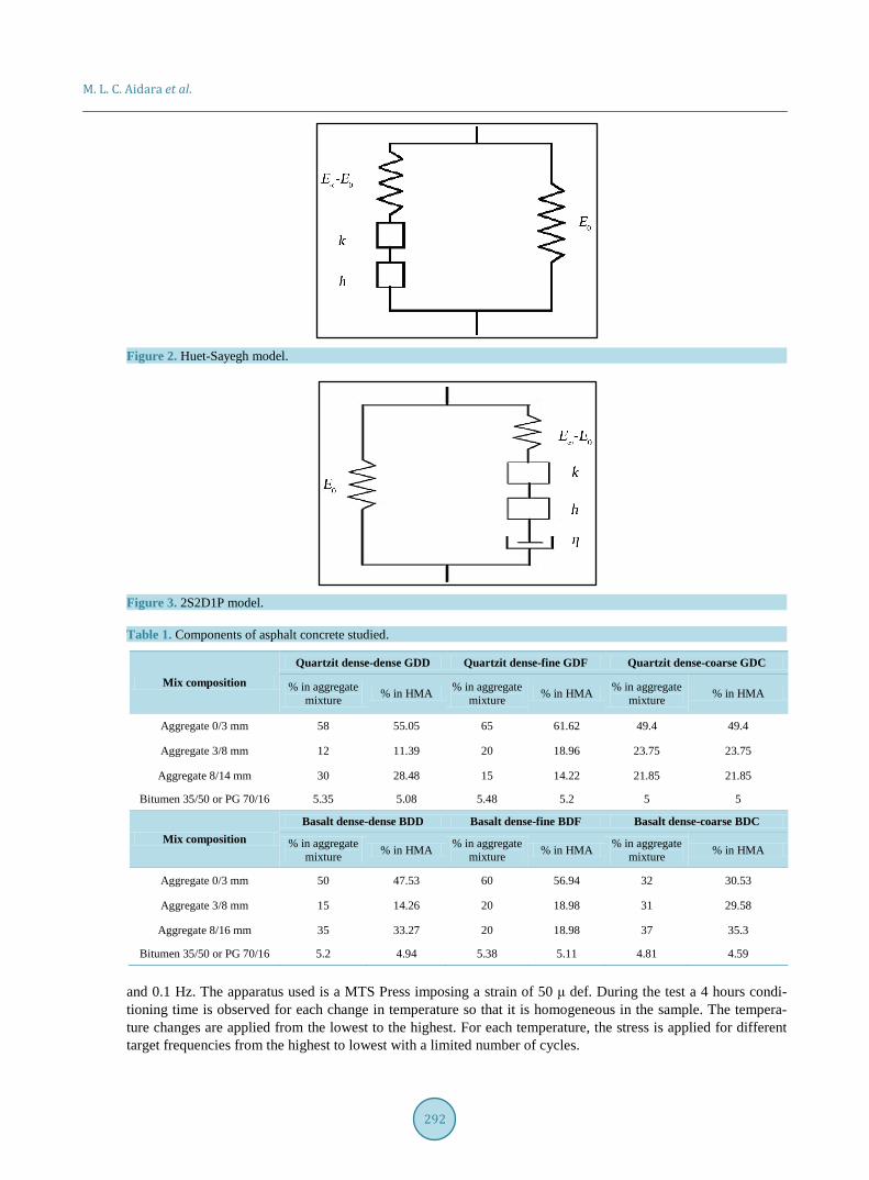
Huet-Sayegh model solve this problem by added a spring in parallel to Huet model [8]. The spring represents

M. L. C. Aidara et al.

291

Figure 1. Huet model.

the static modulus [9] (Figure 2). Equation (2) shows the express of complex modulus by the Huet-Sayegh model.

( ) ( )* 0

01 i ik h

E EE Eδ ωτ ωτ

∞− −

−= +

+ + (2)

with (i) the complex number defined by i2 = −1; ω = 2π frequency, pulsation; E∞: limit the complex modulus when ωτ → ∞; E0 the static modulus of spring; h, k: exponents such that 0 1k h< < < ; δ: dimensionless con-stant; τ: time characteristic whose value varies only with temperature. As Huet model, Huet-Sayegh model is characterized by a continuous spectral.

Di Benedetto and colleagues [10] developed the 2S2P1D model. The model is obtained by added a linear dashpot in series to Huet-Sayegh model (Figure 3). The 2S2P1D model improves the Huet-Sayegh model at high temperatures and low frequencies [9].

Equation (3) shows the express of complex modulus by the 2S2P1D model.

( )( ) ( ) ( )

* 00 1i

1 i i ik hE EE Eωτ

δ ωτ ωτ ωβτ∞

− − −

−= +

+ + + (3)

where (i) is the complex number defined by i2 = −1; *ω = 2π frequency pulse; k, h are exponents such that 0 1k h< < < ; E0 (“static module”) when the module ωτ → 0; E∞ (“glassy modulus”) when the module ωτ → ∞; τ: time characteristic, whose value depends only on the temperature; β: dimensionless constant; η: viscosity Newtonian; ( )0E Eη βτ∞= − . When ωτ → 0, then ( ) ( )*

0 0i iE E E Eωτ ω βτ∞→ + − .

2.2. Complex Modulus Test and Results Visualization The complex modulus test is used to measure the dynamic modulus |E*| of asphalt concrete named “Hot Mixture Asphalt” (HMA) at different temperatures and loading frequencies. The test can be conducted in a uniaxial or triaxial condition in either compression or tension. However, the majority of tests during the past years were in compression [12]. When the test is conducted in compression, the specimen experiences creep, in addition to the dynamic response. In the analysis of results, the creep response is typically ignored and the dynamic modulus is taken as the ratio of the amplitude of the dynamic stress to the amplitude of the dynamic strain. The tension/ compression test on cylindrical specimen belongs to the homogeneous tests, i.e. it makes it possible to obtain directly the linear viscoelastic behavior through the complex modulus. The principle of this test consists in soli- citing in traction and compression a cylindrical specimen in a continuous way according to a sinusoidal signal (traction/compression) centered on zero and applied according to the axial direction of the specimen. In the case of a complex modulus test, a low number of cycles are applied to various frequencies [13]. Complex modulus tests were performed using the Direct Traction-Compression (DTC) test on cylindrical samples according to Canadian and European standards (LC 26-700 and NF EN 12697-26, respectively). Six mixtures (Table 1) were studied (BDC, BDD BDF, GDC, GDD and GDF). Each formula undergoes measurements at temperatures of 0˚C, 10˚C, 20˚C, 30˚C, 40˚C and 55˚C and for each temperature the frequencies are 10 Hz, 5 Hz, 1 Hz, 0.3 Hz

M. L. C. Aidara et al.

292

Figure 2. Huet-Sayegh model.

Figure 3. 2S2D1P model. Table 1. Components of asphalt concrete studied.

Mix composition

Quartzit dense-dense GDD Quartzit dense-fine GDF Quartzit dense-coarse GDC

% in aggregate mixture % in HMA % in aggregate

mixture % in HMA % in aggregate mixture % in HMA

Aggregate 0/3 mm 58 55.05 65 61.62 49.4 49.4

Aggregate 3/8 mm 12 11.39 20 18.96 23.75 23.75

Aggregate 8/14 mm 30 28.48 15 14.22 21.85 21.85

Bitumen 35/50 or PG 70/16 5.35 5.08 5.48 5.2 5 5

Mix composition Basalt dense-dense BDD Basalt dense-fine BDF Basalt dense-coarse BDC

% in aggregate mixture % in HMA % in aggregate

mixture % in HMA % in aggregate mixture % in HMA

Aggregate 0/3 mm 50 47.53 60 56.94 32 30.53

Aggregate 3/8 mm 15 14.26 20 18.98 31 29.58

Aggregate 8/16 mm 35 33.27 20 18.98 37 35.3

Bitumen 35/50 or PG 70/16 5.2 4.94 5.38 5.11 4.81 4.59

and 0.1 Hz. The apparatus used is a MTS Press imposing a strain of 50 μ def. During the test a 4 hours condi-tioning time is observed for each change in temperature so that it is homogeneous in the sample. The tempera-ture changes are applied from the lowest to the highest. For each temperature, the stress is applied for different target frequencies from the highest to lowest with a limited number of cycles.

M. L. C. Aidara et al.

293

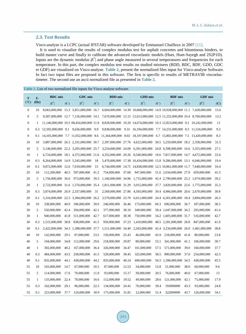
2.3. Test Results Visco-analyse is a LCPC (actual IFSTAR) software developed by Emmanuel Chailleux in 2007 [11].

It is used to visualize the results of complex modulus test for asphalt concretes and bituminous binders, to build master curve and finally to calibrate the advanced viscoelastic models (Huet, Huet-Sayegh and 2S2P1D). Inputs are the dynamic modulus |E*| and phase angle measured in several temperatures and frequencies for each temperature. In this part, the complex modulus test results on studied mixtures (BDD, BDC, BDF, GDD, GDC et GDF) are visualized on Visco-analyse. Table 2, present the normalized files input for Visco-analyse Software. In fact two input files are proposed in this software. The first is specific to results of METRAVIB viscoelas- timeter. The second use an ascii normalized file as presented in Table 2.

Table 2. List of two normalized file inputs for Visco-analyse software.

T (˚C)

F. (Hz)

BDC mix GDC mix BDD mix GDD mix BDF mix GDF mix

|E*| δ(˚) |E*| δ(˚) |E*| δ(˚) |E*| δ(˚) |E*| δ(˚) |E*| δ(˚)

0 10 8,063,000,000 15.3 5,851,000,000 16.7 6,604,000,000 14.39 10,668,000,000 14.9 10,028,000,000 11.1 7,428,000,000 15.6

0 5 9,587,000,000 12.7 7,126,000,000 14.1 7,670,000,000 12.15 12,613,000,000 12.5 11,255,000,000 10.4 8,760,000,000 13.2

0 1 11,146,000,000 10.5 08,454,000,000 11.9 8,828,000,000 10.20 14,674,000,000 10.3 12,823,000,000 9.2 10,242,000,000 11

0 0.3 12,592,000,000 9.1 9,636,000,000 9.9 9,838,000,000 9.31 16,194,000,000 7.7 14,231,000,000 8.3 11,516,000,000 9.3

0 0.1 14,105,000,000 7.7 11,052,000,000 8.6 11,364,000,000 8.02 18,107,000,000 6.7 15,802,000,000 7.5 13,420,000,000 8.3

10 10 3,887,000,000 26.3 2,331,000,000 30.7 2,397,000,000 27.76 4,622,000,000 30.5 5,259,000,000 18.2 2,358,000,000 31.5

10 5 5,146,000,000 22.2 3,205,000,000 25.7 3,254,000,000 24.09 6,391,000,000 24.8 6,398,000,000 16.6 3,355,000,000 27.1

10 1 6,724,000,000 18.1 4,372,000,000 21.6 4,352,000,000 20.26 8,540,000,000 19.6 7,817,000,000 14.7 4,672,000,000 22.6

10 0.3 8,264,000,000 14.9 5,545,000,000 18 5,470,000,000 17.38 10,434,000,000 15.8 9,286,000,000 13.1 6,046,000,000 19.4

10 0.1 9,872,000,000 12.6 7,018,000,000 15 6,744,000,000 14.71 14,838,000,000 12.5 10,861,000,000 11.7 7,648,000,000 16.4

20 10 112,200,000 40.5 597,000,000 41.2 754,000,000 37.68 947,000,000 51.6 2,034,000,000 27.9 659,000,000 41.5

20 5 1,756,000,000 36.6 973,000,000 39.3 1,166,000,000 34.96 1,715,000,000 45.4 2,799,000,000 25.2 1,074,000,000 39.2

20 1 2,722,000,000 31.6 1,576,000,000 35.4 1,811,000,000 31.29 3,015,000,000 37.7 3,820,000,000 22.6 1,775,000,000 35.3

20 0.3 3,874,000,000 26.9 2,337,000,000 31 2,569,000,000 27.86 4,593,000,000 30.4 4,906,000,000 20.6 2,670,000,000 30.8

20 0.1 5,316,000,000 22.3 3,384,000,000 26.2 3,579,000,000 23.70 6,611,000,000 24.4 6,301,000,000 18.4 3,894,000,000 26.3

30 10 338,000,000 40.9 186,000,000 39.9 246,000,000 36.46 173,000,000 60.3 696,000,000 36.7 187,000,000 38.3

30 5 550,000,000 42.4 294,000,000 42.1 377,000,000 38.10 349,000,000 58.4 1,047,000,000 34.2 293,000,000 41.4

30 1 940,000,000 41.8 511,000,000 42.7 617,000,000 38.38 750,000,000 54.2 1,605,000,000 31.7 516,000,000 42.7

30 0.3 1,515,000,000 38.8 838,000,000 41.5 950,000,000 37.23 1,410,000,000 48.5 2,281,000,000 28.8 847,000,000 41.9

30 0.1 2,422,000,000 34.3 1,388,000,000 37.7 1,511,000,000 34.40 2,563,000,000 41.4 3,234,000,000 26.0 1,461,000,000 38.8

40 10 142,000,000 29.5 87,000,000 23.5 150,000,000 25.43 46,000,000 45.9 218,000,000 41.8 80,000,000 23.8

40 5 194,000,000 34.8 112,000,000 29.6 218,000,000 29.87 80,000,000 53.1 341,000,000 41.1 106,000,000 30.7

40 1 302,000,000 40.2 167,000,000 36.4 326,000,000 34.47 161,000,000 57.5 571,000,000 39.0 160,000,000 37.7

40 0.3 484,000,000 43.5 258,000,000 41.5 529,000,000 38.45 325,000,000 58.5 890,000,000 37.0 254,000,000 42.3

40 0.1 835,000,000 44.1 438,000,000 44.2 835,000,000 40.24 690,000,000 56.5 1,396,000,000 34.5 438,000,000 45.5

55 10 103,000,000 14.7 67,000,000 10.5 87,000,000 12.53 34,000,000 15.8 51,000,000 38.0 60,000,000 9.6

55 5 114,000,000 17.6 70,000,000 11.9 93,000,000 15.17 39,000,000 20.5 76,000,000 40.0 67,000,000 13

55 1 133,000,000 22.4 78,000,000 16.6 112,000,000 19.52 49,000,000 28.6 121,000,000 42.1 75,000,000 17.9

55 0.3 162,000,000 29.1 96,000,000 22.5 134,000,000 24.41 70,000,000 39.4 193000000 43.3 93,000,000 24.8

55 0.1 223,000,000 37.7 124,000,000 30.9 175,000,000 31.81 12,000,000 51.4 322000000 43.7 126,000,000 34.1

M. L. C. Aidara et al.

294

In the first columns we find the temperatures number, the frequencies number. Data are then rows in temper-atures blocks. For each line we find successively, temperature, frequency, dynamic modulus and phase angle. The units are ˚C, Hz, Pa and degree.

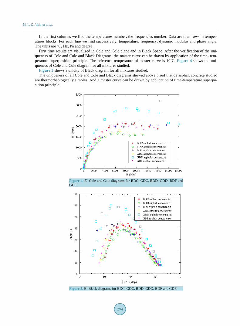
First time results are visualized in Cole and Cole plane and in Black Space. After the verification of the uni-queness of Cole and Cole and Black Diagrams, the master curve can be drawn by application of the time- tem-perature superposition principle. The reference temperature of master curve is 10˚C. Figure 4 shows the uni-queness of Cole and Cole diagram for all mixtures studied.

Figure 5 shows a unicity of Black diagram for all mixtures studied. The uniqueness of all Cole and Cole and Black diagrams showed above proof that de asphalt concrete studied

are thermorheologically simples. And a master curve can be drawn by application of time-temperature superpo- sition principle.

Figure 4. E* Cole and Cole diagrams for BDC, GDC, BDD, GDD, BDF and GDF.

Figure 5. E* Black diagrams for BDC, GDC, BDD, GDD, BDF and GDF.

M. L. C. Aidara et al.

295

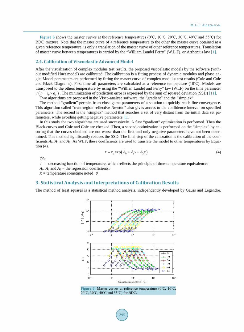
Figure 6 shows the master curves at the reference temperatures (0˚C, 10˚C, 20˚C, 30˚C, 40˚C and 55˚C) for BDC mixture. Note that the master curve of a reference temperature to the other the master curve obtained at a given reference temperature, is only a translation of the master curve of other reference temperatures. Translation of master curve between temperatures is carried by the “William Landel Ferry” (W.L.F). or Arrhenius law [1].

2.4. Calibration of Viscoelastic Advanced Model After the visualization of complex modulus test results, the proposed viscoelastic models by the software (with-out modified Huet model) are calibrated. The calibration is a fitting process of dynamic modulus and phase an-gle. Model parameters are performed by fitting the master curve of complex modulus test results (Cole and Cole and Black Diagrams). First time all parameters are calculated at a reference temperature (10˚C). Models are transposed to the others temperature by using the “Willian Landel and Ferry” law (WLF) on the time parameter ( )0 Taτ τ τ= × . The minimization of prediction error is expressed by the sum of squared deviation (SSD) [11]. Two algorithms are proposed in the Visco-analyse software, the “gradient” and the “simplex”. The method “gradient” permits from close game parameters of a solution to quickly reach fine convergence.

This algorithm called “trust-region reflective Newton” also gives access to the confidence interval on specified parameters. The second is the “simplex” method that searches a set of very distant from the initial data set pa-rameters, while avoiding getting negative parameters [11].

In this study the two algorithms are used successively. A first “gradient” optimization is performed. Then the Black curves and Cole and Cole are checked. Then, a second optimization is performed on the “simplex” by en-suring that the curves obtained are not worse than the first and only negative parameters have not been deter-mined. This method significantly reduces the SSD. The final step of the calibration is the calibration of the coef-ficients A0, A1 and A2. As WLF, these coefficients are used to translate the model to other temperatures by Equa-tion (4).

( )0 0 1 2exp A A x A xτ τ= + + (4)

Où: τ = decreasing function of temperature, which reflects the principle of time-temperature equivalence; A0, A1 and A2 = the regression coefficients; X = temperature sometime noted θ .

3. Statistical Analysis and Interpretations of Calibration Results The method of least squares is a statistical method analysis, independently developed by Gauss and Legendre.

Figure 6. Master curves at reference temperature (0˚C, 10˚C, 20˚C, 30˚C, 40˚C and 55˚C) for BDC.

M. L. C. Aidara et al.

296

Method is used to compare the experimental data, usually tainted by measurement errors with a mathematical model meant to describe these data [14]. In our case the models studied are complex functions predicting the complex modulus of asphalt concretes (Huet model, Huet-Sayegh model and 2S2P1D model).

The method consists of a prescription (initially empirical) which is the function ( ),f x θ which describes “best” data is the one that minimizes the quadratic sum of the deviations of measurements with the predictions of ( ),f x θ . For example, if we have N measurements, (yi) i = 1, N the “optimal” parameters θ within the meaning of

the least squares method are those which minimize the quantity [14]: where ri(θ) are the residues to the model, i.e. the differences between the measurement points (yi) and the model (x; θ).

S(θ) or (SSD) presented in Equation (5) can be considered as a measure of the distance between the experi- mental data and the theoretical model that predicts such data. Prescription least squares command that this dis- tance is minimal [14].

( ) ( )( ) ( )2

1 1;

N N

i i ii i

S y f x rθ θ θ= =

= − =∑ ∑ (5)

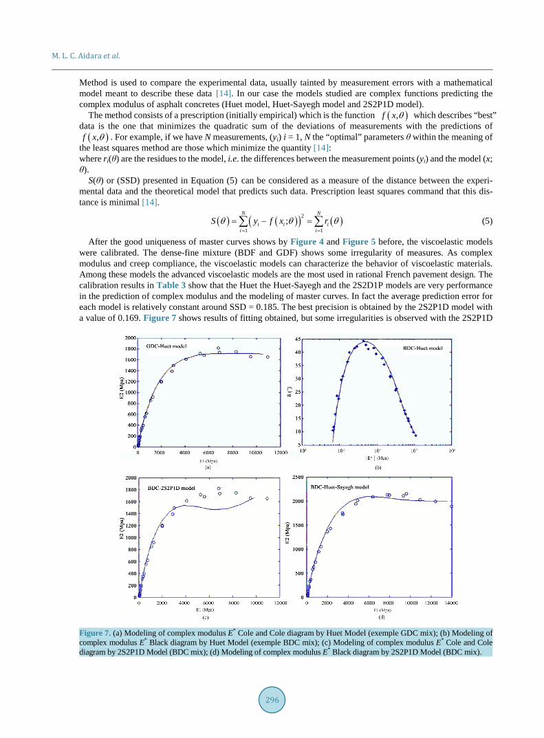
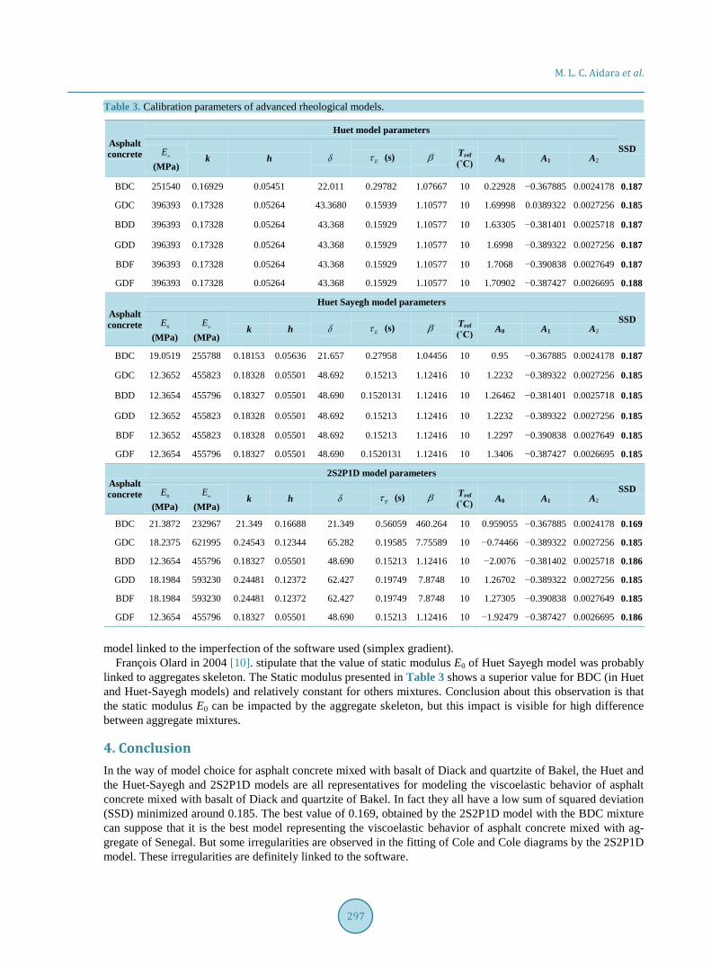
After the good uniqueness of master curves shows by Figure 4 and Figure 5 before, the viscoelastic models were calibrated. The dense-fine mixture (BDF and GDF) shows some irregularity of measures. As complex modulus and creep compliance, the viscoelastic models can characterize the behavior of viscoelastic materials. Among these models the advanced viscoelastic models are the most used in rational French pavement design. The calibration results in Table 3 show that the Huet the Huet-Sayegh and the 2S2D1P models are very performance in the prediction of complex modulus and the modeling of master curves. In fact the average prediction error for each model is relatively constant around SSD = 0.185. The best precision is obtained by the 2S2P1D model with a value of 0.169. Figure 7 shows results of fitting obtained, but some irregularities is observed with the 2S2P1D

Figure 7. (a) Modeling of complex modulus E* Cole and Cole diagram by Huet Model (exemple GDC mix); (b) Modeling of complex modulus E* Black diagram by Huet Model (exemple BDC mix); (c) Modeling of complex modulus E* Cole and Cole diagram by 2S2P1D Model (BDC mix); (d) Modeling of complex modulus E* Black diagram by 2S2P1D Model (BDC mix).

M. L. C. Aidara et al.

297

Table 3. Calibration parameters of advanced rheological models.

Asphalt concrete

Huet model parameters

SSD E∞ (MPa)

k h δ Eτ (s) β Tref (˚C) A0 A1 A2

BDC 251540 0.16929 0.05451 22.011 0.29782 1.07667 10 0.22928 −0.367885 0.0024178 0.187

GDC 396393 0.17328 0.05264 43.3680 0.15939 1.10577 10 1.69998 0.0389322 0.0027256 0.185

BDD 396393 0.17328 0.05264 43.368 0.15929 1.10577 10 1.63305 −0.381401 0.0025718 0.187

GDD 396393 0.17328 0.05264 43.368 0.15929 1.10577 10 1.6998 −0.389322 0.0027256 0.187

BDF 396393 0.17328 0.05264 43.368 0.15929 1.10577 10 1.7068 −0.390838 0.0027649 0.187

GDF 396393 0.17328 0.05264 43.368 0.15929 1.10577 10 1.70902 −0.387427 0.0026695 0.188

Asphalt concrete

Huet Sayegh model parameters

SSD 0E

(MPa) E∞

(MPa) k h δ Eτ (s) β Tref

(˚C) A0 A1 A2

BDC 19.0519 255788 0.18153 0.05636 21.657 0.27958 1.04456 10 0.95 −0.367885 0.0024178 0.187

GDC 12.3652 455823 0.18328 0.05501 48.692 0.15213 1.12416 10 1.2232 −0.389322 0.0027256 0.185

BDD 12.3654 455796 0.18327 0.05501 48.690 0.1520131 1.12416 10 1.26462 −0.381401 0.0025718 0.185

GDD 12.3652 455823 0.18328 0.05501 48.692 0.15213 1.12416 10 1.2232 −0.389322 0.0027256 0.185

BDF 12.3652 455823 0.18328 0.05501 48.692 0.15213 1.12416 10 1.2297 −0.390838 0.0027649 0.185

GDF 12.3654 455796 0.18327 0.05501 48.690 0.1520131 1.12416 10 1.3406 −0.387427 0.0026695 0.185

Asphalt concrete

2S2P1D model parameters

SSD 0E

(MPa) E∞

(MPa) k h δ Eτ (s) β Tref

(˚C) A0 A1 A2

BDC 21.3872 232967 21.349 0.16688 21.349 0.56059 460.264 10 0.959055 −0.367885 0.0024178 0.169

GDC 18.2375 621995 0.24543 0.12344 65.282 0.19585 7.75589 10 −0.74466 −0.389322 0.0027256 0.185

BDD 12.3654 455796 0.18327 0.05501 48.690 0.15213 1.12416 10 −2.0076 −0.381402 0.0025718 0.186

GDD 18.1984 593230 0.24481 0.12372 62.427 0.19749 7.8748 10 1.26702 −0.389322 0.0027256 0.185

BDF 18.1984 593230 0.24481 0.12372 62.427 0.19749 7.8748 10 1.27305 −0.390838 0.0027649 0.185

GDF 12.3654 455796 0.18327 0.05501 48.690 0.15213 1.12416 10 −1.92479 −0.387427 0.0026695 0.186

model linked to the imperfection of the software used (simplex gradient).

François Olard in 2004 [10]. stipulate that the value of static modulus E0 of Huet Sayegh model was probably linked to aggregates skeleton. The Static modulus presented in Table 3 shows a superior value for BDC (in Huet and Huet-Sayegh models) and relatively constant for others mixtures. Conclusion about this observation is that the static modulus E0 can be impacted by the aggregate skeleton, but this impact is visible for high difference between aggregate mixtures.

4. Conclusion In the way of model choice for asphalt concrete mixed with basalt of Diack and quartzite of Bakel, the Huet and the Huet-Sayegh and 2S2P1D models are all representatives for modeling the viscoelastic behavior of asphalt concrete mixed with basalt of Diack and quartzite of Bakel. In fact they all have a low sum of squared deviation (SSD) minimized around 0.185. The best value of 0.169, obtained by the 2S2P1D model with the BDC mixture can suppose that it is the best model representing the viscoelastic behavior of asphalt concrete mixed with ag-gregate of Senegal. But some irregularities are observed in the fitting of Cole and Cole diagrams by the 2S2P1D model. These irregularities are definitely linked to the software.

M. L. C. Aidara et al.

298

Acknowledgements The authors would like to acknowledge Professor Meissa FALL (RIP) for his guidance and valuable input in this research project; and the “Mapathé NDIOUCK Enterprise” for supporting the high price shipping of aggregates from Senegal to Canada.

References [1] Di Benedetto, H.V. and Corté, F. (2005) Materials (Vol. 2) (H. Science, Éd.). Lavoisier, Lyon. [2] Huang, Y.H. (2004) Pavement Analysis and Design. PEARSON, Prentice Hall, Kentucky. [3] Carter, A. and Perraton, D. (2002) Measurement of Complex Modulus Asphalt Concretes. 2nd Material Specialty

Conference of the Canadian Society for Civil Engineering, Montréal. [4] Yoder, E.J. and Witczak, M.W. (1975) Principle of Pavement Design. 2nd Edition, John Wiley & Sons, Hoboken, 711

p. http://dx.doi.org/10.1002/9780470172919 [5] NCHRP, TRB, NRC (2004) Guide for Mechanistic—Empirical Design—For New and Rehabilitated Pavement Structure.

ARA, Inc, ERES Consultants Division, Illinois. [6] LCPC—SETRA (1994) Conception and Pavement Design. Technical Guid. [7] Huet, C. (1963) Etude par une méthode d’impédance du comportement viscoélastique des matériaux hydrocarbonés.

Thèse de Docteur Ingénieur, Faculté des Sciences de l’université de Paris, Paris, 69 p. [8] Sayegh, G. (1965) Variation des modules de quelques bitumes purs et bétons bitumineux. Thèse de Doctorat

d’Ingénieur, Faculté des Sciences de l’université de Paris. [9] Olard, F. and DiBenedetto, H. (2002) General 2S2P1D Model and Relation between the Linear Viscoelastic Behaviors

of Bituminous Binders and Mixes. Road Materials and Pavement Design. [10] Olard, F. (2004) Thermomechanical Behavior of Asphalt Mixtures at Low Temperature. Unpublished Doctoral Disser-

tation. [11] Chailleux, E. (2007) User Manual of Visco-Analysis Software. LCPC. [12] Papagiannakis, A.T. and Masad, E.A. (2007) Pavement Design and Materials. John Wiley and Sons, Inc., Hoboken, NJ,

552 p. [13] Touhara, R. (2012) Studies of Fatigue Resistance of Asphalt Mixtures. Master Thesis, Superior School of Technology,

Montreal. [14] Techno Sciences. http://www.techno-science.net/?onglet=glossaire&definition=6004