CIRJE Discussion Papers can be downloaded without charge from:

http://www.cirje.e.u-tokyo.ac.jp/research/03research02dp.html

Discussion Papers are a series of manuscripts in their draft form. They are not intended for

circulation or distribution except as indicated by the author. For that reason Discussion Papers may

not be reproduced or distributed without the written consent of the author.

CIRJE-F-778

Choice of Collateral Currency

Masaaki FujiiGraduate School of Economics, University of Tokyo

Akihiko TakahashiUniversity of Tokyo

December 2010

Choice of Collateral Currency ∗

Masaaki Fujii†, Akihiko Takahashi‡

First version: 19 April 2010Current version: 7 December 2010

Abstract

Collateral has been used for a long time in the cash market and we have alsoexperienced significant increase of its use as an important credit risk mitigation toolin the derivatives market for this decade. Despite its long history in the financialmarket, its importance for funding has been recognized relatively recently followingthe explosion of basis spreads in the crisis. This paper has demonstrated the impact ofcollateralization on derivatives pricing through its funding effects based on the actualdata of swap markets. It has also shown the importance of the ”choice” of collateralcurrency. In particular, when a contract allows multiple currencies as eligible collateralas well as its free replacement, the paper has found that the embedded ”cheapest-to-deliver” option can be quite valuable and significantly change the fair value of a trade.The implications of these findings for risk management have been also discussed.

Keywords : swap, collateral, derivatives, Libor, currency, OIS, EONIA, Fed-Fund, CCS,basis, risk management, HJM, FX option, CSA, CVA, term structure

∗Forthcoming in Risk Magazine. This research is supported by CARF (Center for Advanced Researchin Finance) and the global COE program “The research and training center for new development inmathematics.” All the contents expressed in this research are solely those of the authors and do notrepresent the view of any institutions. The authors are grateful to Yasufumi Shimada, a manager ofShinsei Bank, and also Fujii’s former colleagues of Morgan Stanley, especially those in Tokyo office forfruitful discussions. The contents of the paper do not represent any views or opinions of Shinsei Bank norMorgan Stanley. The authors are not responsible or liable in any manner for any losses and/or damagescaused by the use of any contents in this research.

†Graduate School of Economics, The University of Tokyo‡Graduate School of Economics, The University of Tokyo

1

1 Introduction

Collateralization in the OTC (over-the-counter) market has continued to grow at a rapidpace over the past decade. According to ISDA (International Swaps and DerivativesAssociation), about 70% of the trade volumes for all the OTC trades were collateralizedat the end of 2009, which was merely 30% in 2003 [4]. A stringent collateral managementwill also be a crucial issue for successful installation of central clearing houses.

The role of collateralization is mainly twofold: 1) reduction of the counterparty creditrisk, and 2) change of funding costs of trades. The first one has been well recognized andstudied extensively. Although it is not as obvious as the first one, the second effect is alsoimportant. Recently, the latter effect has gained strong attention among practitioners,since they have experienced significant difference between Libors and funding costs ofcollateralized trades. The work of Johannes & Sundaresan (2007) [5] was the first focusingon the cost of collateralization, which studied the effect on swap prices based on empiricalanalysis. As a more recent work, Piterbarg (2010) [6] discussed the general option pricingusing the similar formula to take the funding cost of collateral into account.

The impacts of collateralization are the most significant in interest rate and long datedFX markets, where they affect various types of basis spread and also FX forward. In previ-ous two works Fujii, Shimada & Takahasi (2009)[1, 2], we have extended the formula usedin [5, 6] to the situation where the payment and collateral currencies are different, which iscrucial to handle multi-currency products. Based on the result, we have presented system-atic procedures of curve construction in the presence of collateral and multiple currencies,and also their no-arbitrage dynamics in an HJM (Heath-Jarrow-Morton) framework.

In this article, we have constructed the collateralized swap curves consistently withthe actual market data, and demonstrated the importance of collateralization in pricingof derivatives 1. It is well-known among market participants that the existence of largebasis spreads in cross currency swap (CCS) market is reflecting differences in funding costsamong various currencies. Hence, it is a natural question to ask what is the impact onderivative pricing from different choice of collateral currency. In fact, by making use of theinformation in CCS markets, we have found that the choice of the collateral currency hasnon-negligible impact on derivative prices. This finding gives rise to another interestingtwist. When the relevant CSA (credit support annex, which specifies all the details ofcollateral agreement) allows multiple choices of collateral currency and free replacementamong them, a payer of the collateral has the ”cheapest-to-deliver” (CTD) option. Wehave demonstrated the embedded option can significantly change the effective discountingfactor and hence the fair value of the trade, especially when the CCS market is volatile.

2 Pricing under the collateralization

This section reviews [1], our results on pricing derivatives under the collateralization. Letus make the following simplifying assumptions about the collateral contract.

1. Full collateralization (zero threshold) by cash.2. The collateral is adjusted continuously with zero minimum transfer amount.

1All the market data used in this article were taken from the Bloomberg.

2

Actually, daily margin call is now quite popular in the market, which makes the above as-sumptions a reasonable proxy for the reality. Since the assumptions allow us to neglect theloss given default of the counterparty, we can treat each trade/payment separately with-out worrying about the non-linearity arising from the netting effects and the asymmetrichandling of exposure.

We consider a derivative whose payoff at time T is given by h(i)(T ) in terms of currency”i”. We suppose that currency ”j” is used as the collateral for the contract. Note thatinstantaneous return (or cost when it is negative ) by holding the cash collateral at timet is given by

y(j)(t) = r(j)(t) − c(j)(t) , (2.1)

where r(j) and c(j) denote the risk-free interest rate and the collateral rate of the currencyj, respectively. A common practice in the market is to set c(j) as the overnight (ON) rateof currency j. Distinction between the theoretical risk-free rate and the market ON rateis required for unified treatment of different collaterals and also for calibration to a crosscurrency basis, which will become clearer in later discussions. If we denote the presentvalue of the derivative at time t by h(i)(t) (in terms of currency i), collateral amountposted from the counterparty is given by

(h(i)(t)/f (i,j)

x (t)), where f

(i,j)x (t) is the foreign

exchange rate at time t representing the price of the unit amount of currency j in termsof currency i. These considerations lead to the following calculation for the collateralizedderivative price,

h(i)(t) = EQi

t

[e−∫ T

t r(i)(s)dsh(i)(T )]

+ f (i,j)x (t)EQj

t

[∫ T

te−∫ s

t r(j)(u)duy(j)(s)

(h(i)(s)

f(i,j)x (s)

)ds

],

where EQi

t [·] is the time t conditional expectation under the risk-neutral measure of cur-rency i, where the money-market account of currency i is used as the numeraire. Byaligning the measure in the above formula, it is easy to see that

X(t) := e−∫ t0 r(i)(s)dsh(i)(t) +

∫ t

0e−∫ s0 r(i)(u)duy(j)(s)h(i)(s)ds (2.2)

is a Qi-martingale under appropriate integrability conditions. This tells us that the processof the option price can be written as

dh(i)(t) =(r(i)(t) − y(j)(t)

)h(i)(t)dt + dM(t) (2.3)

with some Qi-martingale M .As a result, we have the following theorem:

Theorem 1 2 Suppose that h(i)(T ) is a derivative’s payoff at time T in terms of currency”i” and that currency ”j” is used as the collateral for the contract. Then, the value of thederivative at time t, h(i)(t) is given by

h(i)(t) = EQi

t

[e−∫ T

t r(i)(s)ds(e∫ T

t y(j)(s)ds)

h(i)(T )]

(2.4)

= D(i)(t, T )ET i

t

[e−∫ T

t y(i,j)(s)dsh(i)(T )]

, (2.5)2Although we are dealing with continuous processes here, we obtain the same result as long as there is

no simultaneous jump of underlying assets when the counterparty defaults.

3

wherey(i,j)(s) = y(i)(s) − y(j)(s) (2.6)

with y(i)(s) = r(i)(s) − c(i)(s) and y(j)(s) = r(j)(s) − c(j)(s). Here, we have defined thecollateralized zero-coupon bond of currency i as

D(i)(t, T ) = EQi

t

[e−∫ T

t c(i)(s)ds]

. (2.7)

We have also defined the ”collateralized forward measure” T i of currency i, for which ET i

t [·]denotes the time t conditional expectation where D(i)(t, T ) is used as its numeraire 3.

As a corollary of the theorem, we have

h(t) = EQt

[e−∫ T

t c(s)dsh(T )]

= D(t, T )ETt [h(T )] (2.8)

when the payment and collateral currencies are the same. This is consistent with theresult of Piterbarg (2010) [6]. In addition, by setting h(T ) = 1, it is easily seen by (2.5)that ET i

t

[e−∫ T

t y(i,j)(s)ds]

is the ratio of two discount bonds, i.e. a relative value of thediscount bond collateralized in a different currency j in terms of the one collateralized inits payment currency i.

3 Curve Construction in Single Currency

In this section, we will construct the relevant yield curves in a single currency market. Forthe details of the procedures, see [1, 3]. Here, we briefly summarize the set of formulasneeded to strip the relevant discounting factors and forward Libors;

OISN

N∑n=1

∆nD(0, Tn) = D(0, T0) − D(0, TN ) ,

IRSM

M∑m=1

∆mD(0, Tm) =M∑

m=1

δmD(0, Tm)ETm [L(Tm−1, Tm; τ)] ,

N∑n=1

δnD(0, Tn)(ETn [L(Tn−1, Tn; τS)] + TSN

)=

M∑m=1

δmD(0, Tm)ETm [L(Tm−1, Tm; τL)] .

These are the consistency conditions to give the market quotes of various swaps 4. Wehave denoted the market observed OIS (Overnight Index Swap) rate, IRS (Interest RateSwap) rate and TS (Tenor Swap) spread respectively as OISN , IRSM and TSN , wherethe subscripts represent the lengths of swaps. {Tn}n≥0 are the reset/payment times ofeach instrument. We distinguish day-count fraction of fixed and floating legs by ∆ andδ, which are not necessarily the same among different instruments. L(Tm−1, Tm; τ) is theLibor with tenor τ whose reset and payment times are Tm−1 and Tm, respectively. Inthe third formula, we have distinguished the two different tenors by τS and τL (> τS). IfτS = 3m and τL = 6m, for example, then N = 2M to match the length of two legs.

3Notice the difference from the usual forward measure where the numeraire is not collateralized.4If payments are compounded in TS, the formula becomes slightly more complicated. However, the

effect from compounding is negligibly small and does not cause any meaningful change to the result.

4

Figure 1: USD zero rate curves of Fed-Fund rate, 3m and 6m Libors.

In Fig. 1, we have given examples of calibrated yield curves for USD market on2009/3/3 and 2010/3/16, where ROIS, R3m and R6m denote the zero rates for OIS (Fed-Fund rate), 3m and 6m forward Libor, respectively. ROIS(·) is defined as ROIS(T ) =− ln(D(0, T ))/T . For the forward Libor, the zero-rate curve Rτ (·) is determined recur-sively through the relation

ETm [L(Tm−1, Tm; τ)] =1

δm

(e−Rτ (Tm−1)Tm−1

e−Rτ (Tm)Tm− 1

). (3.1)

In the actual calculation of D(0, ·), we have used the Fed-Fund vs 3m-Libor basis swap,where the two parties exchange 3m Libor and the compounded Fed-Fund rate with spread,which seems more liquid and a larger number of quotes available than the usual OIS. InFig. 2, one can see the historical behavior of the spread between 1yr IRS and OIS forUSD, JPY and EUR, where the underlying floating rates of IRS are 3m-Libor for USDand EUR and 6m-Libor for JPY.

Remarks: In the above calculations, we have assumed that the conditions given inthe previous section are satisfied, and also that all the instruments are collateralized bythe cash of domestic currency or its payment currency. Cautious readers may worryabout the possibility that the market quotes contain significant contributions from marketparticipants who use a foreign currency as collateral. However, the induced changes inIRS/TS quotes are very small and impossible to distinguish from the bid/offer spreads innormal circumstances, because the correction appears both in the fixed and floating legswhich keeps the market quotes almost unchanged 5.

5As for cross currency swaps, the change can be a few bps, which can be comparable to the marketbid/offer spreads.

5

Figure 2: Difference between 1yr IRS and OIS. Underlying floating rates are 3m-Libor forUSD and EUR, and 6m-Libor for JPY.

4 Curve Construction in Multiple Currencies

4.1 Calibration Procedures

In this section, we will discuss how to make the term structure consistent with CCS (crosscurrency swap) market. The current market is dominated by USD crosses where 3m USDLibor flat is exchanged with 3m Libor of a different currency with additional basis spread.The most popular type of CCS is called MtMCCS in which the notional of USD leg isreset at the start of every calculation period of Libor while the notional of the other legis kept constant throughout the contract period 6.

We consider a MtMCCS of (i, j) currency pair, where the leg of currency i (intended tobe USD) needs notional refreshments. We assume that the collateral is posted in currencyi, which seems common in the market.

The value of j-leg of a T0-start TN -maturing MtMCCS is calculated as

PVj = −D(j)(0, T0)ET j0

[e−∫ T00 y(j,i)(s)ds

]+ D(j)(0, TN )ET j

n

[e−∫ TN0 y(j,i)(s)ds

]+

N∑n=1

δ(j)n D(j)(0, Tn)ET j

n

[e−∫ Tn0 y(j,i)(s)ds

(L(j)(Tn−1, Tn; τ) + BN

)], (4.1)

where the basis spread BN is available as a market quote. In [2], we have assumed thatall of the {y(k)(·)} and hence {y(i,j)(·)} are deterministic functions of time to make thecurve construction simpler. Here, we slightly relax the assumption allowing randomness

6As for the details of MtMCCS and a different type of CCS, see [2, 3].

6

of {y(i,j)(·)}. As long as we assume that {y(i,j)(·)} is independent from the dynamics ofLibors and collateral rates, the procedures of bootstrapping given in [2] can be applied inthe same way 7. Under this assumption, we obtain

PVj = −D(j)(0, T0)e−∫ T00 y(j,i)(0,s)ds + D(j)(0, TN )e−

∫ TN0 y(j,i)(0,s)ds

+N∑

n=1

δ(j)n D(j)(0, Tn)e−

∫ Tn0 y(j,i)(0,s)ds

(ET j

n [L(j)(Tn−1, Tn; τ)] + BN

). (4.2)

Here, we have defined, y(j,i)(t, s), the forward rate of y(j,i)(s) at time t as 8

e−∫ T

t y(j,i)(t,s)ds = EQj

t

[e−∫ T

t y(j,i)(s)ds]

. (4.3)

Note that non-zero correlations among {y(i,k)}i,k themselves do not pose any difficulty oncurve construction.

On the other hand, the present value of i-leg in terms of currency j is given by

PVi = −N∑

n=1

EQi

[e−∫ Tn−10 c(i)(s)dsf (i,j)

x (Tn−1)]

/f (i,j)x (0)

+N∑

n=1

EQi[e−∫ Tn0 c(i)(s)dsf (i,j)

x (Tn−1)(1 + δ(i)

n L(i)(Tn−1, Tn; τ))]

/f (i,j)x (0)

=N∑

n=1

δ(i)n D(i)(0, Tn)ET i

n

[f

(i,j)x (Tn−1)

f(i,j)x (0)

B(i)(Tn−1, Tn; τ)

], (4.4)

where

B(i)(t, Tk; τ) = ET i

kt

[L(i)(Tk−1, Tk; τ)

]− 1

δ(i)k

(D(i)(t, Tk−1)D(i)(t, Tk)

− 1

), (4.5)

which represents a Libor-OIS spread. Since we found no persistent correlation between FXand Libor-OIS spread in historical data, we have treated them as independent variables.Even if a non-zero correlation exists in a certain period, the expected correction seemsnot numerically important relative to the typical size of bid/offer spreads for MtMCCS(about a few bps at the time of writing). Since 3-month timing adjustment of FX is safelynegligible, an approximate value of i-leg is obtained as

PVi ≃N∑

n=1

δ(i)n D(i)(0, Tn)

D(j)(0, Tn−1)D(i)(0, Tn−1)

e−∫ Tn−10 y(j,i)(0,s)dsB(i)(0, Tn; τ), (4.6)

where we have used the following result of the forward FX collateralized with currency i:

f (i,j)x (t, T ) = f (i,j)

x (t)D(j)(t, T )D(i)(t, T )

e−∫ T

t y(j,i)(t,s)ds . (4.7)

7In practice, it would not be a problem even if there is a non-zero correlation as long as it does notmeaningfully change the model implied quotes compared to the market bid/offer spreads.

8Since we are assuming the independence from the collateral rate, the measure change within the samecurrency gives no difference.

7

Using Eqs. (4.2) and (4.6), the term structure of {y(j,i)(0, ·)} can be extracted from theequality PVi = PVj , a consistency condition for the observed market spread.

Under the above approximation, (i, j)-MtMCCS par spread is expressed as

BN =

N∑

n=1

δ(i)n D

(i)Tn

D(j)Tn−1

D(i)Tn−1

e−∫ Tn−10 y(j,i)(0,s)dsB

(i)Tn

−N∑

n=1

δ(j)n D

(j)Tn

e−∫ Tn0 y(j,i)(0,s)dsB

(j)Tn

−

N∑n=1

D(j)Tn−1

e−∫ Tn−10 y(j,i)(0,s)ds

(e−∫ Tn

Tn−1y(j,i)(0,s)ds − 1

)]/

N∑n=1

δ(j)n D

(j)Tn

e−∫ Tn0 y(j,i)(0,s)ds , (4.8)

where we have shortened the notations as D(k)(0, T ) = D(k)T and B(k)(0, T ; τ) = B

(k)T .

4.2 Historical Behavior

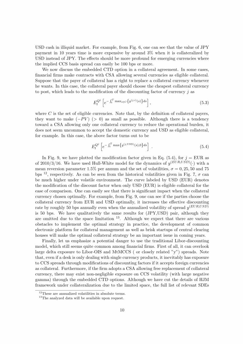
Now, let us check the historical behavior of Ry(EUR,USD) and Ry(JPY,USD) given in Fig. 3to 5 9. Here, the spread Ry is defined as

Ry(j,i)(T ) = −ln(EQj

[e−∫ T0 y(j,i)(s)ds

])T

=1T

∫ T

0y(j,i)(0, s)ds . (4.9)

In Fig. 3, we have shown historical behaviors of basis spreads of 5y MtMCCS, correspond-ing Ry(X,USD)(5y), and difference of R3m(5y) − ROIS(5y) between the two currency pairsdenoted by ∆Libor-OIS(5y; USD, X) 10. Here, ”X” stands for either EUR or JPY. Asexpected from Eq. (4.8), Ry(X,USD)(5y) + ∆Libor-OIS(5y; USD, X) well agrees with the5y MtMCCS spread with typical error smaller than a few bps. From the figure, we ob-serve that a significant portion of the movement of CCS spreads stems from the changeof y(i,j), rather than the difference of Libor-OIS spread between two currencies. In fact,the level (difference)-correlation between Ry and CCS spread is quite high, which is about93% (69%) for EUR and about 70% (48%) for JPY for the historical series used in thefigure. On the other hand, the same quantities between ∆Libor-OIS and CCS spread aregiven by −56% (3%) for EUR and 9% (4%) for JPY.

The 3m-roll historical volatilities of y(EUR,USD) instantaneous forwards, which areannualized in absolute terms, are given in Fig. 7. In a calm market, they tend to be 50bps or so, but they were more than a percentage point just after the market crisis, whichis reflecting a significant widening of the CCS basis spread to seek USD cash in illiquidmarket. Except the CCS basis spread, y does not seem to have persistent correlationswith other market variables such as OIS, IRS and FX forwards.

5 Implications for Derivatives Pricing and Summary

We now consider implications of collateralization for derivatives pricing. It is straight-forward to see when payment and collateral currencies are the same. As in Eq. (2.8),

9Due to the lack of OIS data for JPY market, we have only a limited data for (JPY,USD) pair. Wehave used Cubic Monotone Spline for calibration although the figures are given in linear plots for ease.

10It can be interpreted as the difference of Libor-OIS spread between USD and X.

8

Figure 3: Ry(EUR,USD)(5y), Ry(JPY,SD)(5y), difference of Libor-OIS spreads, and corre-sponding quotes of 5y-MtMCCS.

discounting rate is now determined by collateral (or ON) rate rather than Libors. Hence,in the presence of the current level of Libor-OIS spread of (10 ∼ 20)bps, the conventionalLibor discounting method results in significant underestimation of the value of future pay-ments, which can even be a few percentage points for long maturities. Considering themechanism of collateralization, financial firms need to hedge the move of OIS in additionto Libors. In particular, the risk of floating-rate payments needs to be checked carefully,since the overnight rate can move in the opposite direction to Libor as was observed inthis financial crisis. In Fig. 8, the present values of Libor floating legs with final principal(= 1) payment

PV =N∑

n=1

δnD(0, Tn)ETn [L(Tn−1, Tn; τ)] + D(0, TN ) (5.1)

are given for various maturities. If traditional Libor discounting is used, the stream ofLibor payments has the constant present value ”1”, which is obviously wrong from ourresults. This point is very important in risk-management point of view, since financial firmsmay overlook the quite significant interest-rate risk exposure when they use traditionalinterest rate models in their system.

If a trade with payment currency j is collateralized by foreign currency i, an additionalmodification to the discounting factor appears (See theorem1 with h(T ) = 1.) 11:

e−∫ T

t y(j,i)(t,s)ds = EQj

t

[e−∫ T

t y(j,i)(s)ds]

. (5.2)

From Figs. 5 and 6, one can see that posting USD as collateral tends to be expensive fromthe view point of collateral payers, which is particularly the case when everyone seeking

11Here, we are assuming independence of y from reference assets.

9

USD cash in illiquid market. For example, from Fig. 6, one can see that the value of JPYpayment in 10 years time is more expensive by around 3% when it is collateralized byUSD instead of JPY. The effects should be more profound for emerging currencies wherethe implied CCS basis spread can easily be 100 bps or more.

We now discuss the embedded CTD option in a collateral agreement. In some cases,financial firms make contracts with CSA allowing several currencies as eligible collateral.Suppose that the payer of collateral has a right to replace a collateral currency wheneverhe wants. In this case, the collateral payer should choose the cheapest collateral currencyto post, which leads to the modification of the discounting factor of currency j as

EQj

t

[e−∫ T

t maxi∈C{y(j,i)(s)}ds], (5.3)

where C is the set of eligible currencies. Note that, by the definition of collateral payers,they want to make (−PV ) (> 0) as small as possible. Although there is a tendencytoward a CSA allowing only one collateral currency to reduce the operational burden, itdoes not seem uncommon to accept the domestic currency and USD as eligible collateral,for example. In this case, the above factor turns out to be

EQj

t

[e−∫ T

t max{y(j,USD)(s),0}ds]

. (5.4)

In Fig. 9, we have plotted the modification factor given in Eq. (5.4), for j = EUR asof 2010/3/16. We have used Hull-White model for the dynamics of y(EUR,USD)(·) with amean reversion parameter 1.5% per annum and the set of volatilities, σ = 0, 25, 50 and 75bps 12, respectively. As can be seen from the historical volatilities given in Fig. 7, σ canbe much higher under volatile environment. The curve labeled by USD (EUR) denotesthe modification of the discount factor when only USD (EUR) is eligible collateral for theease of comparison. One can easily see that there is significant impact when the collateralcurrency chosen optimally. For example, from Fig. 9, one can see if the parties choose thecollateral currency from EUR and USD optimally, it increases the effective discountingrate by roughly 50 bps annually even when the annualized volatility of spread y(EUR,USD)

is 50 bps. We have qualitatively the same results for (JPY,USD) pair, although theyare omitted due to the space limitation 13. Although we expect that there are variousobstacles to implement the optimal strategy in practice, the development of commonelectronic platform for collateral management as well as brisk startups of central clearinghouses will make the optimal collateral strategy be an important issue in coming years.

Finally, let us emphasize a potential danger to use the traditional Libor-discountingmodel, which still seems quite common among financial firms. First of all, it can overlooklarge delta exposure to Libor-OIS and MtMCCS ( or closely related ”y”) spreads. Notethat, even if a desk is only dealing with single currency products, it inevitably has exposureto CCS spreads through modifications of discounting factors if it accepts foreign currenciesas collateral. Furthermore, if the firm adopts a CSA allowing free replacement of collateralcurrency, there may exist non-negligible exposure on CCS volatility (with large negativegamma) through the embedded CTD options. Although we have cut the details of HJMframework under collateralization due to the limited space, the full list of relevant SDEs

12These are annualized volatilities in absolute terms.13The analyzed data will be available upon request.

10

could be provided upon request. We emphasize that every building block of the frameworkis market observable, i.e. collateral rate c(i), Libor-OIS sprad B(i), y(i,j) spread, and f

(i,j)x

for each currency and pairs, where the unobserved risk-free rate is embedded in c and y.See [2] for related discussions.

References

[1] Fujii, M., Shimada, Y., Takahashi, A., 2009, ”A note on construction of multiple swapcurves with and without collateral,” CARF Working Paper Series F-154, available athttp://ssrn.com/abstract=1440633.

[2] Fujii, M., Shimada, Y., Takahashi, A., 2009, ”A Market Model of Interest Rates withDynamic Basis Spreads in the presence of Collateral and Multiple Currencies”, CARFWorking Paper Series F-196, available at http://ssrn.com/abstract=1520618.

[3] Fujii, M., Shimada, Y., Takahashi, A., 2010, ”On the Term Structure of Interest Rateswith Basis Spreads, Collateral and Multiple Currencies”, based on the presentationsgiven at ”International Workshop on Mathematical Finance” at Tokyo, JapaneseFinancial Service Agency, and Bank of Japan.

[4] ISDA Margin Survey 2009 & 2010,Market Review of OTC Derivative Bilateral Collateralization Practices.

[5] Johannes, M. and Sundaresan, S., 2007, ”The Impact of Collateralization on SwapRates”, Journal of Finance 62, 383410.

[6] Piterbarg, V. , 2010, ”Funding beyond discounting : collateral agreements and deriva-tives pricing” Risk Magazine.

11

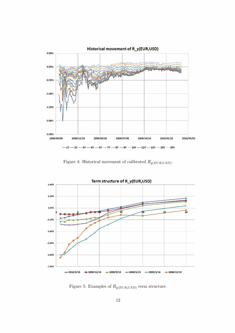
Figure 4: Historical movement of calibrated Ry(EUR,USD).

Figure 5: Examples of Ry(EUR,USD) term structure.

12

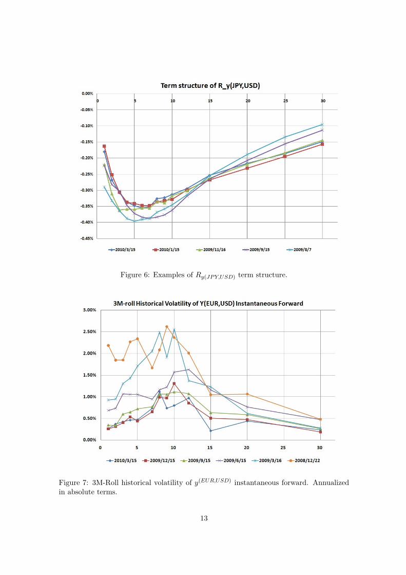
Figure 6: Examples of Ry(JPY,USD) term structure.

Figure 7: 3M-Roll historical volatility of y(EUR,USD) instantaneous forward. Annualizedin absolute terms.

13

Figure 8: Present value of USD Libor stream with final principal (= 1) payment.

Figure 9: Modification of EUR discounting factors based on HW model for y(EUR,USD) asof 2010/3/16. The mean-reversion parameter is 1.5%, and the volatility is given at eachlabel.

14