Choice under Uncertainty

Jonathan Levin

October 2006

1 Introduction

Virtually every decision is made in the face of uncertainty. While we often rely on

models of certain information as you’ve seen in the class so far, many economic

problems require that we tackle uncertainty head on. For instance, how should in-

dividuals save for retirement when they face uncertainty about their future income,

the return on different investments, their health and their future preferences? How

should firms choose what products to introduce or prices to set when demand is

uncertain? What policies should governments choose when there is uncertainty

about future productivity, growth, inflation and unemployment?

Our objective in the next few classes is to develop a model of choice behavior

under uncertainty. We start with the von Neumann-Morgenstern expected utility

model, which is the workhorse of modern economics. We’ll consider the foundations

of this model, and then use it to develop basic properties of preference and choice

in the presence of uncertainty: measures of risk aversion, rankings of uncertain

prospects, and comparative statics of choice under uncertainty.

As with all theoretical models, the expected utility model is not without its

limitations. One limitation is that it treats uncertainty as objective risk – that is,

as a series of coin flips where the probabilities are objectively known. Of course, it’s

hard to place an objective probability on whether Arnold Schwarzenegger would

be a good California governor despite the uncertainty. In response to this, we’ll

discuss Savage’s (1954) approach to choice under uncertainty, which rather than

assuming the existence of objective probabilities attached to uncertain prospects

1

makes assumptions about choice behavior and argues that if these assumptions are

satisfied, a decision-maker must act as if she is maximizing expected utility with

respect to some subjectively held probabilities. Finally we’ll conclude by looking

at some behavioral criticisms of the expected utility model, and where they lead.

A few comments about these notes. First, I’ll stick pretty close to them in

lectures and problem sets, so they should be the first thing you tackle when you’re

studying. That being said, you’ll probably want to consult MWG and maybe

Kreps at various points; I certaintly did in writing the notes. Second, I’ve followed

David Kreps’ style of throwing random points into the footnotes. I don’t expect

you to even read these necessarily, but they might be starting points if you decide

to dig a bit deeper into some of the topics. If you find yourself in that camp, Kreps

(1988) and Gollier (2001) are useful places to go.

2 Expected Utility

We start by considering the expected utility model, which dates back to Daniel

Bernoulli in the 18th century and was formally developed by John von Neumann

and Oscar Morgenstern (1944) in their book Theory of Games and Economic Be-

havior. Remarkably, they viewed the development of the expected utility model

as something of a side note in the development of the theory of games.

2.1 Prizes and Lotteries

The starting point for the model is a set X of possible prizes or consequences. In

many economic problems (and for much of this class), X will be a set of monetary

payoffs. But it need not be. If we are considering who will win Big Game this

year, the set of consequences might be:

X = {Stanford wins, Cal wins, Tie}.

We represent an uncertain prospect as a lottery or probability distribution over

the prize space. For instance, the prospect that Stanford and Cal are equally likely

to win Big Game can be written as p = (1/2, 1/2, 0) . Perhaps these probabilities

2

depend on who Stanford starts at quarterback. In that case, there might be two

prospects: p or p0 = (5/9, 3/9, 1/9), depending on who starts.

We will often find it useful to depict lotteries in the probability simplex, as

shown in Figure 1. To understand the figure, consider the depiction of three-

dimensional space on the left. The point p is meant to represent (1/2, 1/2, 0)

and the point p0 to represent (5/9, 3/9, 1/9). In general, any probability vector

(p1, p2, p3) can be represented in this picture. Of course, to be a valid probability

vector, the probabilities have to sum to 1. The triangle represents the space of

points (p1, p2, p3) with the property that p1 + p2 + p3 = 1. The right hand side

picture simply dispenses with the axes. In the right figure, p and p0 are just as

before. Moving up means increasing the likelihood of the second outcome, moving

down and left the likelihood of the third outcome and so on.

p1

p2

p3

1

1

1

0p p

p1=1

p2=1

p3=1

p’ p’

Figure 1: The Probability Simplex

More generally, given a space of consequences X , denote the relevant set oflotteries over X as P = ∆(X ). Assuming X = {x1, ..., xn} is a finite set, a lotteryover X is a vector p = (p1, ..., pn), where pi is the probability that outcome xi

occurs. Then:

∆(X ) = {(p1, ..., pn) : pi ≥ 0 and p1 + ...+ pn = 1}

3

For the rest of this section, we’ll maintain the assumption that X is a finite set.It’s easy to imagine infinite sets of outcomes – for instance, any real number

between 0 and 1 – and later we’ll wave our hands and behave as if we had

developed the theory for larger spaces of consequences. You’ll have to take it

on faith that the theory goes through with only minor amendments. For those of

you who are interested, and relatively math-oriented, I recommend taking a look

at Kreps (1988).

Observe that given two lotteries p and p0, any convex combination of them:

αp+(1−α)p0 with α ∈ [0, 1] is also a lottery. This can be viewed simply as statingthe mathematical fact that P is convex. We can also view αp + (1 − α)p0 more

explicitly as a compound lottery, summarizing the overall probabilities from two

successive events: first, a coin flip with weight α, 1 − α that determines whether

the lottery p or p0 should be used to determine the ultimate consequences; second,

either the lottery p or p0. Following up on our Big Game example, the compound

lottery is: first the quarterback decision is made, then the game is played.

p

p2=1

p3=1p’

p1=1

αp + (1-α)p’

α

1-α

p

p’

Figure 2: A Compound Lottery

Figure 2 illustrates the idea of a compound lottery as a two-stage process, and as

a mathematical fact about convexity.

4

2.2 Preference Axioms

Naturally a rational decision-maker will have preferences over consequences. For

the purposes of the theory, however, the objects of choice will be uncertain prospects.

Therefore we will assume that the decision-maker has preferences over lotteries on

the space of consequences, that is preferences over elements of P.We start by assuming that the decision maker’s preference relation º on P

is complete and transitive. We then add two additional axioms: continuity and

independence.

Definition 1 A preference relation º on the space of lotteries P is continuousif for any p, p0, p00 ∈ P with p º p0 º p00, there exists some α ∈ [0, 1] such that

αp+ (1− α)p00 ∼ p0.

An implication of the continuity axiom (sometimes called the Archimedean

axiom) is that if p is preferred to p0, then a lottery “close” to p (a short distance

away in the direction of p00 for instance) will still be preferred to p0. This seems

eminently reasonable, though there are situations where it might be doubtful.

Consider the following example. Suppose p is a gamble where you get $10 for sure,

p0 is a gamble where you nothing for sure, and r is a gamble where you get killed

for sure. Naturally p should be strictly preferred to q, which is strictly preferred to

r. But this means that there is some α ∈ (0, 1) such that you would be indifferentbetween getting nothing and getting $10 with probability α and getting killed with

probability 1− α.

Given that preferences are complete, transitive and continuous, they can be

represented by a utility function U : P → R, where p º p0 if and only if U(p) ≥U(p0). Our next axiom, which is more controversial, will allow us to say a great

deal about the structure of U . This axiom is the key to expected utility theory.

Definition 2 A preference relation º on the space of lotteries P satisfies inde-pendence if for all p, p0, p00 ∈ P and α ∈ [0, 1], we have

p º p0 ⇔ αp+ (1− α)p00 º αp0 + (1− α)p00.

5

The independence axiom says that I prefer p to p0, I’ll also prefer the possibility

of p to the possibility of p0, given that the other possibility in both cases is some

p00. In particular, the axiom says that if I’m comparing αp + (1 − α)p00 to αp0 +

(1 − α)p00, I should focus on the distinction between p and p0 and hold the same

preference independently of both α and p00. This axiom is sometimes also called

the substitution axiom: the idea being that if p00 is substituted for part of p and

part of p0, this shouldn’t change my ranking.

Note that the independence axiom has no counterpart in standard consumer

theory. Suppose I prefer {2 cokes, 0 twinkies} to {0 cokes, 2 twinkies}. Thisdoesn’t imply that I prefer {2 cokes, 1 twinkie} to {1 coke, 2 twinkies}, even thoughthe latter two are averages of the first two bundles with {2 cokes, 2 twinkies}.The independence axiom is a new restriction that exploits the special structure of

uncertainty.

2.3 Expected Utility

We now introduce the idea of an expected utility function.

Definition 3 A utility function U : P → R has an expected utility form (or is

a von Neumann-Morgenstern utility function) if there are numbers (u1, ..., un) for

each of the N outcomes (x1, ..., xn) such that for every p ∈ P, U(p) =Pn

i=1 pi · ui.

If a decision maker’s preferences can be represented by an expected utility

function, all we need to know to pin down her preferences over uncertain outcomes

are her payoffs from the certain outcomes x1, ..., xn.

Crucially, an expected utility function is linear in the probabilities, meaning

that:

U(αp+ (1− α)p0) = αU(p) + (1− α)U(p0). (1)

It is not hard to see that this is in fact the defining property of expected utility. If

a utility function is linear in the probabilities, so that (1) holds for every p, p0 and

α, then it must have an expected utility form (try proving this).

In standard choice theory, a big deal is made about the fact that utility functions

are ordinal. A decision maker with utility function U and one with utility function

6

V = g ◦ U for some increasing function g have the same preferences. The same

is not true of expected utility. Expected utility do satisfy the weaker property,

however, that they are preserved by affine (increasing linear) transformations.

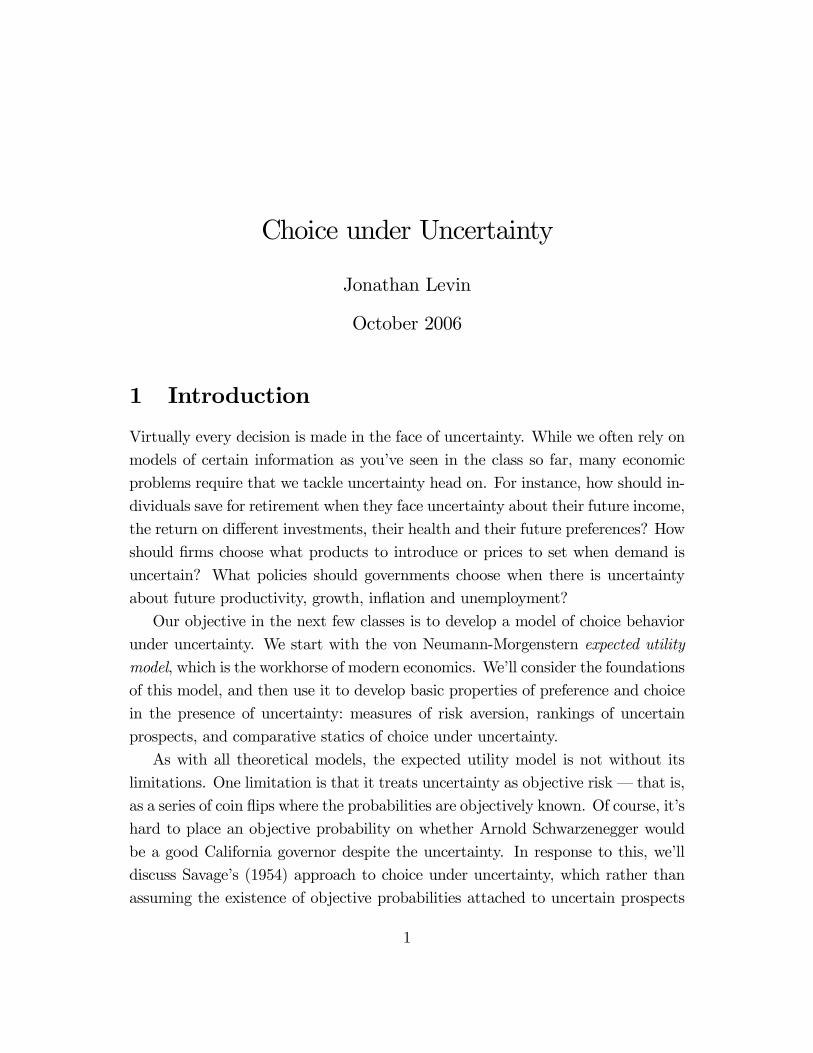
Proposition 1 Suppose that U : P → R is an expected utility representation of thepreference relation º on P. Then V : P → R is an expected utility representationof º if and only if there are scalars a and b > 0 such that V (p) = a+ bU(p) for all

p ∈ P.

Proof. Suppose U is an expected utility representation of º, and U(p) =P

i piui.

(⇐) Suppose V = a + bU . Because b > 0, if U(p0) ≥ U(p), then clearly

V (p0) ≥ V (p), so V also represents º. Moreover, V has an expected utility form

because, if we define vi = a+ bui for all i = 1, ..., n, then:

V (p) = a+ bU(p) = a+ b ·nXi=1

piui =nXi=1

pi(a+ bui) =nXi=1

pivi.

(⇒) Suppose V is an expected utility representation of º. Let p, p ∈ P be

lotteries such that p º p º p for all p ∈ P. (The fact there there is a “best” and“worst” lottery follows immediately from the fact that we have assumed a finite

number of lotteries. With an infinite number of lotteries, we’d need to be a bit

more clever to ensure best and worst lotteries or work around their absence.) If

p ∼ p, then both U and V are constant over P and the result is trivial. So assumep  p. Then given p ∈ P, there exists some λp ∈ [0, 1] such that:

U(p) = λpU(p) + (1− λp)U(p).

Therefore:

λp =U(p)− U(p)

U(p)− U(p).

Now, because p ∼ λpp+ (1− λp)p, we have:

V (p) = V (λpp+ (1− λp)p)

= λpV (p) + (1− λp)V (p).

Defining

a = V (p)− U(p)b and b =V (p)− V (p)

U(p)− U(p),

it is easy to check that V (p) = a+ bU(p). Q.E.D.

7

2.4 A Representation Theorem

Our next result says that a complete and transitive preference relation º on Pcan be represented by a utility function with an expected utility form if and only

if it satisfies the two axioms of continuity and independence.1 To the extent that

one accepts the continuity and independence axioms (not to mention completeness

and transitivity) as a description of how people should (or do) behave, this is

remarkable.

Theorem 1 (von Neumann and Morgenstern, 1947) A complete and transitive

preference relation º on P satisfies continuity and independence if and only if it

admits a expected utility representation U : P → R.

The idea is actually pretty straightforward. Let’s suppose there are just three

possible outcomes x1, x2 and x3, so that lotteries can be represented in the two-

dimensional simplex. We now draw indifference curves in the simplex. (See Figure

3 below.)

If the decision-maker’s preferences can be represented by an expected utility

function, the linearity of expected utility means that her indifference curves must

be parallel straight lines. Why? Because if U(p) = U(p0) then the fact that

U(αp+(1−α)p0) = αU(p)+(1−α)U(p0)means that U must be constant on the lineconnecting p and p0. This same linearity property also implies that the indifference

curves must be parallel. Conversely if U were not linear in the probabilities,

the indifferences curves would not be parallel straight lines. That is, given a

utility representation, having indifference curves that are parallel straight lines is

equivalent to having an expected utility representation.

The idea behind the theorem is that given the other axioms, the independence

axiom is also equivalent to having indifference curves that are parallel straight

lines, and hence equivalent to having preferences that are representable by a vN-M

expected utility function.

1Remember that X is finite. In that case where X is infinite, this statement needs (in additionto some technical stuff) a small amendment. To get expected utility, we need one extra axiom:

the sure thing principle. It essentially says that if p is concentrated on a subset B ⊂ X , and everycertain outcome in B is preferred to q, then p is preferred to q.

8

Why is independence the same as parallel straight indifference curves? Well, if

p ∼ p0, then by independence p ∼ αp + (1 − α)p0 ∼ p0, so the indifference curves

must be straight lines. Moreover, if indifference curves are not parallel, then we

must have situation as in Figure 3, where p0 ∼ p and but 12p0 + 1

2p00 Â 1

2p + 1

2p00.

Thus the independence axiom implies that indifference curves are parallel straight

lines.

x1x3

x2

x1x3

x2

Increasing preference

p’

p

Increasing preference

p’’

p

p’

Figure 3: Independence implies Parallel Linear Indifference Curves

A Formal Proof. I’ll leave it to you to check that if U is an expected utility

representation of º, then º must satisfy continuity and independence, and insteadfocus on the harder part of the proof.

Let º be given and assume it satisfies continuity and independence. We will

construct an expected utility function U that represents º. As above, let p, p ∈ Pbe the most and least preferred lotteries in P. If p ∼ p, then any constant function

represents º and the result is trivial, so assume p  p.

Step 1. As a preliminary step, observe that if 1 > β > α > 0, then by the

independence axiom:

p  βp+ (1− β)p  αp+ (1− α)p  p.

9

Why is this? For the first inequality, write the left hand side as βp + (1 − β)p.

Because p  p, the independence axiom immediately generates the inequality. For

the second inequality, write the left hand side as (β−α)p+αp+(1− β)p and the

right hand side as (β − α)p + αp + (1 − β)p, and again invoke independence. A

similar argument works for the third inequality.

Step 2. Now, I claim that for any p ∈ P, there exists a unique λp such that:

λpp+ (1− λp)p ∼ p. (2)

Because p º p º p, some such λp exists as a consequence of continuity. The

previous step means it is unique.

Step 3. Finally, I claim that the utility function U(p) = λp is an expected

utility representation of º. To see that U represents º, observe that:

p º q ⇔ λpp+ (1− λp)p º λqp+ (1− λq)p ⇔ λp ≥ λq.

To see that U has an expected utility form, we want to prove that for any α ∈ [0, 1]and p, p0 ∈ P :

U(αp+ (1− α)p0) = αU(p) + (1− α)U(p0).

We know that:

p ∼ U(p)p+ (1− U(p))p

p0 ∼ U(p0)p+ (1− U(p0))p.

Therefore, by the indepedence axiom (twice), and by re-arranging terms (noting

that the second and third expressions represent the same point in the probability

simplex):

αp+ (1− α)p0 ∼ α¡U(p)p+ (1− U(p))p

¢+ (1− α)p0

∼ α¡U(p)p+ (1− U(p))p

¢+ (1− α)

¡U(p0)p+ (1− U(p0))p

¢∼ (αU(p) + (1− α)U(p0)) p+ (1− αU(p)− (1− α)U(p0)) p.

Therefore, using the definition of U :

U(αp+ (1− α)p0) = αU(p) + (1− α)U(p0),

which completes the proof. Q.E.D.

10

2.5 Digression: Expected Utility and Social Choice

An interesting by-product of the development of expected utility theory was a new

justification for utilitarianism proposed by Vickrey, Arrow and especially Harsanyi

(1955). The idea of utilitarian social decisions, dating back at least to Jeremy

Bentham, is that society should try to maximizeP

i Ui, where U1, ..., Un were

the utility functions of the different individuals in the society. Clearly such an

approach pre-supposes both that individual utilities are cardinal and that they are

interpersonally comparable. That is, one can say that Mr. A should give Mr. B a

dollar because the dollar matters more to to B than it does to A.

The idea that individual utilities are cardinal and comparable came under heavy

fire in the 1930s, notably from Lionel Robbins at the London School of Economics.

In response, Abraham Bergson (1938, written while he was a Harvard undergradu-

ate!) proposed that even if one could not defend the utilitarian approach, it might

still make sense to maximize a welfare function W (U1, ..., Un), where W would be

increasing in all its arguments. Bergson argued that this approach does not re-

quire cardinality or interpersonal comparability. It does presume the existence of a

complete and transitive social preference over alternatives,2 and also some notion

of Pareto optimality: if Mr. A can be made better off without hurting anyone else,

this is a good thing.

After expected utility theory appeared in the 1940s, Harsanyi (1955) suggested

refining Bergson’s approach by defining social preferences over uncertain outcomes

rather than just sure outcomes. Harsanyi showed that if both individuals and

society have preferences that satisfy the vN-M axioms, then (subject to a weak

“individualistic” assumption about social preferences), social choices should be

made according to some social welfare functionP

aiUi, where each Ui is a vN-M

individual utility. In this case, the utilities are cardinal (as we have seen above)

but not interpersonally comparable. Harsanyi argued, however, that this problem

could be overcome by re-scaling using the ai’s. Thus the vN-M approach provided

a way to resurrect classical utilitarianism.

2If you know some social choice theory, and are familiar with Condorcet’s Paradox (i.e. the

idea that majority voting can lead to cycles), you will know that even transitivity of socialpreferences is not a trivial assumption.

11

Harsanyi’s basic line of thinking was social judgments should be made “behind

the veil of ignorance.” One should imagine being placed with equal probability

in the position of any individual in society, and evaluate social alternatives from

that viewpoint. If one’s preferences regarding social policies from this position of

uncertainty follow the vN-M axioms, this leads one to the utilitarian approach.

3 Risk Aversion

We’re now going to study expected utility in the special case where prizes are in

dollars. To this end, assume that the prize space X is the real line, or some intervalof it. A lottery is represented by a cumulative distribution function F (·), whereF (x) is the probability of receiving less than or equal to x dollars.

If U is an expected utility representation of preferences, then for all F ,

U(F ) =

Zu(x)dF (x).

MWG refer to u as the Bernoulli utility function and U as the von Neumann-

Morgenstern utility function. We’ll adopt this terminology and also go ahead and

make the fairly natural assumption that u is increasing and continuous.

3.1 Money Lotteries and Risk Aversion

Let’s define δx to be a degenerate lottery that gives x for certain.

Definition 4 A decision-maker is (strictly) risk-averse if for any non-degeneratelottery F (·) with expected value EF =

RxdF (x), the decision-maker (strictly)

prefers δEF to F .

Risk-aversion says that:Zu(x)dF (x) ≤ u

µZxdF (x)

¶for all F .

This mathematical expression goes by the name Jensen’s inequality. It is the

defining property of concave functions. From this, it follows that:

12

Proposition 2 A decision-maker is risk-averse if and only if u is concave.

Figure 4(a) gives some graphical intuition. Consider a lottery that is equally

likely to pay 1 or 3, and compare it to a lottery that pays 2 for certain. Evidently,

if u is concave, the certain outcome is better. If u is linear, they give the same

expected utility. If u is convex, the risky prospect gives higher expected utility.

x1 2 3

u(2)u(F)

x

u(2)u(p)

(a) (b)

c(F,u)

Figure 4: Illustration of Risk-Aversion

3.2 Measuring Risk Aversion

For a risk-averse decision-maker, getting EF for sure is weakly preferred to the

lottery F and perhaps strictly preferred. This raises the question of exactly how

many certain dollars F is worth.

Definition 5 The certain equivalent c(F, u) is the amount of dollars such that:

u(c(F, u)) =

Zu(x)dF (x).

13

Figure 4(b) represents the certain equivalent on the x-axis. Note that whenever u

is concave c(F, u) ≤ EF .

Certain equivalents provide an intuitive way to measure the degree of risk-

aversion. Suppose we have two decision-makers, one with Bernoulli utility function

u and one with Bernoulli utility function v. It seems quite natural to say that u is

more risk-averse than v if for all lotteries F , c(F, u) ≤ c(F, v).

Of course, this is not the only way to think about one decision-maker being

more risk-averse than another. Arrow (1971) and Pratt (1964) offered another way

to think about measuring risk aversion, based on the local curvature of the utility

function.

Definition 6 For any twice differentiable Bernoulli utility function u(·), theArrow-Pratt coefficient of absolute risk aversion is A(x) = −u00(x)/u0(x).

Our next result shows the equivalence of several definitions of “more risk-

averse”.

Proposition 3 (Pratt, 1964) The following definitions of u being “more risk averse”than v are equivalent:

1. Whenever u prefers a lottery F to some certain outcome δx, then v does as

well.

2. For every F , c(F, u) ≤ c(F, v).

3. The function u is “more concave” than v: there exists some increasing con-

cave function g such that u = g ◦ v.

4. For every x, A(x, u) ≥ A(x, v).

Proof. The equivalence of (1) and (2) should be pretty clear. Now, because u andv are both monotone, there must be some increasing function g such that u = g◦v.For the rest:

(2)⇔ (3). Using the definition of c(·, ·) and substituting for u = g ◦ v :

u(c(F, u)) ≤ u(c(F, v)) ⇔Z

g(v(x))dF (x) ≤ g

µZv(x)dF (x)

¶14

The second inequality is Jensen’s and hold if and only if g is concave.

(3)⇔ (4). By differentiating:

u0(x) = g0(v(x))v0(x)

and

u00(x) = g00(v(x))v0(x)2 + g0(v(x))v00(x)

Dividing the second expression by the first, we obtain:

A(x, u) = A(x, v)− g00(u(x))

g0(u(x))v0(x).

It follows that A(x, u) ≥ A(x, v) for all x if and only if g00 ≤ 0. Q.E.D.

3.3 Risk Preferences and Wealth Levels

An important issue that comes up often in economic modelling is how risk prefer-

ences change with wealth. Suppose that Bill Gates and I are identical, but for the

extra $50 billion in his savings account. It seems natural that simply by virtue of

this one difference, if I would prefer a certain risky gamble to, say, $100 for sure,

then Bill would also prefer the risky gamble. This is captured by the notion of

decreasing absolute risk-aversion.

Definition 7 The Bernoulli utility function u(·) has decreasing (constant, in-creasing) absolute risk-aversion if A(x, u) is a decreasing (constant, increas-ing) function of x.

Let F ⊕x denote the lottery F with the certain amount x added to each prize.

The implications of DARA should be pretty clear from Proposition 2 above. If my

preferences satisfy DARA and I prefer F to some certain amount x, then I will

prefer F ⊕ z to the certain amount x+ z for any z > 0. Or, put another way, if I

prefer F to x for some initial wealth level z, I’ll prefer F to x for any higher initial

wealth level z0.

A second useful way to make comparisons across wealth levels has to do with

proportionate gambles. Let t be some non-negative random variable with cdf F .

15

Given x ≥ 0, a proportionate gamble pays tx. Intuitively, you start with initialwealth x and the gamble pays a random rate of return t.

We can define a certain equivalent for rates of return, t̂ = cr(F, x, u) such that:

u(t̂x) =

Zu(tx)dF (x).

Then t̂ is the certain rate of return such that the agent is just indifferent between

t̂x for sure and the gamble that pays tx when t is distributed as F .

Getting back to comparisons across wealth, we might ask the following question.

Suppose I’m willing now to take a gamble that will cost me 10% of my wealth with

probability 1/2 but will double my wealth with equal probability. Would I also

take this gamble if I was richer? The answer to this question hinges on the notion

of relative risk aversion.

Definition 8 For any twice differentiable Bernoulli utility function u(·), the co-efficient of relative risk aversion at x is R(x) = −xu00(x)/u0(x).

Proposition 4 An agent exhibits decreasing relative risk aversion, i.e. R(x) is

decreasing in x, if and only if cr(F, x, u) is increasing in x.

You can consult MWG for a proof. Note that under DRRA, we get a positive

answer to the question posed a moment ago. If I’m willing to invest 10% of my

wealth in some risky asset, I’d be willing to do the same (i.e. invest 10% of my

wealth in this risky asset) if I were richer.

Note the relation between relative and absolute risk aversion, R(x) = xA(x).

Consider wealth levels x > 0. This means that if an agent has decreasing relative

risk aversion, he must have decreasing absolute risk aversion. By the same token,

if an agent has increasing absolute risk aversion, he must have increasing relative

risk aversion. This is intuitive. Suppose I’m unwilling to invest a fixed amount of

money, say $20, in a risky lottery and this $20 corresponds to 1% of my wealth.

If I have increasing absolute risk aversion, I’d be unwilling to invest this same $20

even if I were wealthier. And if I were wealthier, this $20 would correspond to

less than 1% of my wealth, so I certainly wouldn’t be willing to invest 1% of my

wealth.

We’ll return to absolute and relative risk aversion when we do applications.

16

4 Comparing Risky Prospects

Now that we’ve looked a bit a basic properties of utility functions and made some

comparisons, let’s take a shot at trying to compare different lotteries.

4.1 First Order Stochastic Dominance

A natural question is when one lottery could be said to pay more than another.

This leads to the idea of first order stochastic dominance.

Proposition 5 The distribution G first order stochastically dominates the distri-

bution F if for every x, G(x) ≤ F (x), or equivalently if for every nondecreasing

function u : R→ R,Ru(x)dG(x) ≥

Ru(x)dF (x).

The proposition asserts the equivalence of two similar, but logically distinct

ideas: first, the purely statistical notion that for any x, G is more likely than F

to pay more than x; second, the preference-based notion that any decision-maker

who prefers more to less will necessarily prefer G to F .

Proof. Assuming differentiability, we can integrate by parts:Zu(x)dG(x) = u(x)G(x)|x=∞x=−∞ −

Zu0(x)G(x)dx.

Therefore (being a bit casual and assuming u(x)(G(x)− F (x))→ 0 as x→∞):Zu(x)dG(x)−

Zu(x)dF (x) =

Zu0(x) [F (x)−G(x)] dx.

As u0 ≥ 0, then if F ≥ G for all x, the expression is clearly positive. On the other

hand, if F (x) < G(x) in the neighborhood of some x, we can pick a nondecreasing

function u that is strictly increasing only in the neighborhood of x and constant

elsewhere, so the expression won’t be positive for every nondecreasing u. Q.E.D.

There is at least one other nice characterization of first order stochastic domi-

nance. Suppose we start with the lottery F and construct the following compound

lottery. First we resolve F . Then, if the resolution of F is x, we hold a sec-

ond lottery that can potentially increase, but will never decrease x. Here’s an

17

example: suppose under F the outcome is either 1 or 3 with equal probability.

Suppose whenever the outcome is 3 we add a dollar with probability 1/2. This is

demonstrated in Figure 5 below and is pretty clearly a good thing for anyone with

nondecreasing utility. Now, if we let G denote the distribution of the outcome of

the compound lottery, then G will first order stochastically dominate F . In fact,

the reverse is true as well. If G first order stochastically dominates F , we can start

with F and construct G as a compound lottery where the second stage always

results in upward shifts.

x0

1

2

3

4

1/2

1/2

F(•) G(•)

1/2

1/4

1/4

1 2 3 4

F(•)

0

1/2

1G(•)

Figure 5: A First Order Stochastic Dominance Shift

4.2 Second Order Stochastic Dominance

A second natural question about lotteries is when one lottery is “less risky” than

another. In order to separate differences in risk from differences in expected return,

we will focus on comparing distributions F and G with the same expected payoff,

or same mean.

Proposition 6 Consider two distributions F and G with the same mean. The

distribution G second order stochastically dominates the distribution F if for every

18

x,R x−∞G(y)dy ≤

R x−∞ F (y)dy, or equivalently if for every concave function u :

R→ R,Ru(x)dG(x) ≥

Ru(x)dF (x).

Proof. We want to prove the equivalence of the two definitions. To keep thingssimple, let’s assume u is differentiable and also that there is some x for which

F (x) = G(x) = 1 (this can be relaxed). Recall from above that after integrating

by parts: Zu(x)dG(x)−

Zu(x)dF (x) =

Zu0(x) [F (x)−G(x)] dx. (3)

Now, because F and G have the same mean, another integration by parts implies:ZxdF (x) =

ZxdG(x) ⇔

ZF (x)dx =

ZG(x)dx.

So if we take the first expression, integrate by parts a third time(!), and do some

cancelling, we get:

−Z

u00(x)

∙Z x

−∞F (y)dy −

Z x

−∞G(y)dy

¸dx.

Now u00 ≤ 0, so ifR x−∞ F (y)dy ≥

R x−∞G(y)dy, then clearly the whole expression is

positive and all concave u prefer G to F . Conversely, suppose in the neighborhood

of some x,R x−∞ F (y)dy <

R x−∞G(y)dy. We can take u to be linear below and above

x and strictly concave in the neighborhood of x, so that the expression is negative

and u is a concave utility that prefers F to G.3 Q.E.D.

3Both this proof and the one above rely heavily on integration by part. This is, however, a

general way to prove stochastic dominance theorems that doesn’t require differentiability. Theidea is that given a class of utility functions U (e.g. all non-decreasing functions, all concavefunctions, etc.), it is often possible to find a smaller set of “basis” functions B ⊂ U such thatevery function u ∈ U can be written as a convex combination of functions in B. (If the set B isminimal, the elements of B are “extreme” points of U – think convex sets.) It is then the casethat

RudG ≥

RudF for all u ∈ U if and only if

RudG ≥

RudF for all u ∈ B, so one can focus

on the basis functions to establish statistical conditions on G and F . You can try this yourselffor first order stochastic dominance: let B be the set of “step” functions: i.e. functions equal to0 below some point x and equal to 1 above it. For more, see Gollier (2001); this was also the

topic of Susan Athey’s Stanford dissertation.

19

Rothschild and Stiglitz (1970) introduced a clever way of thinking about “more

risk” in terms of changes to a distribution G that add risk.4 Starting with a

distribution G, we construct the following compound lottery. After G is resolved,

say with outcome x, we add to x some mean-zero random variable. Rothschild

and Stiglitz refer to this as a “mean-preserving spread” because while the new

compound lottery (let’s call it F ) has the same mean, its distribution will be more

“spread out”. Figure 5 has an example. The distribution G is equally likely to

result in a payoff of 1 or 3 dollars. To construct F , whenever the outcome is 3,

we add or subtract a dollar with equal probability. The result is a new lottery

where the probability is more spread out – also note that F and G satisfy the

second-order stochastic dominance statistical property in the above proposition.

x0

1

2

3

4

1/2

1/2

G(•) F(•)

1/2

1/4

1/4

1 2 3 4

F(•)

0

1/2

1 G(•)

Figure 6: A Mean Preserving Spread

It’s pretty easy to check, using Jensen’s inequality, that guys with concave

utility won’t like mean-preserving spreads. Somewhat harder, but still possible,

4Actually, to be historically accurate, all of the second order stochastic dominance ideas wereworked out long before, in a book by Hardy, Littlewood and Polya (1934). Rothschild and Stiglitzhit on them independently and their paper brought these ideas to the attention of economists.

20

is to show that whenever G second order stochastically dominates F , F can be

obtained from G through a sequence of mean preserving spreads. So this provides

an alternative characterization of second order stochastic dominance.

5 Applications and Comparative Statics

Now that we’ve developed some basic properties of utility functions and lotteries,

we’re going to look at two important examples: insurance and investment. In the

process, we’ll try to point out some important comparative statics results for choice

problems under uncertainty.

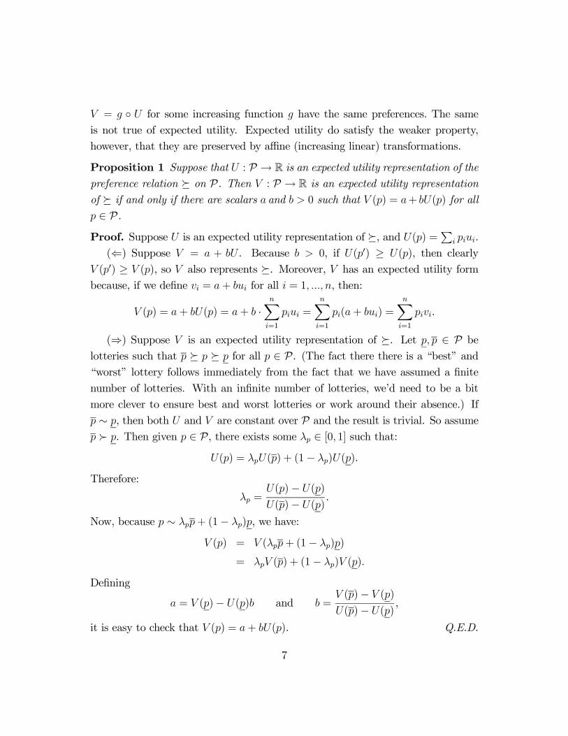
5.1 The Demand for Insurance

Consider an agent with wealth w, who faces a probability p of incurring a loss L.

She can insure against this loss by buying a policy that will pay out in the event

the loss occurs. A policy that will pay a in the event of loss costs qa dollars. How

much insurance should she buy?

Writing this as an optimization problem under uncertainty:

maxa

pu(w − qa− L+ a) + (1− p)u(w − qa).

Denoting the objective function by U(a), the first order condition is:

dU

da= pu0(w − qa− L+ a)(1− q)− (1− p)u0(w − qa)q = 0.

Assuming u is concave (so our consumer is risk-averse), this is necessary and suffi-

cient for a solution. The first order condition simply says that the marginal benefit

of an extra dollar of insurance in the bad state times the probability of loss equals

the marginal cost of the extra dollar of insurance in the good state.

We say that insurance is actuarily fair if the expected payout of the insurance

company just equals the cost of insurance, that is if q = p. We might expect a

competitive insurance market to deliver actuarily fair insurance. In this event, the

first-order condition simplifies to:

u0(w − qa− L+ a) = u0(w − qa),

21

meaning that the consumer should fully insure and set a = L. In this case, she

is completely covered against loss. This result – that a risk-averse consumer will

always fully insure if insurance prices are actuarily fair – turns out to be quite

important in many contexts.

What happens if the price of insurance is above the actuarily fair price, so

q > p. Assuming an interior solution, the optimal coverage a∗ satisfies the first

order condition:u0(w − qa− L+ a)

u0(w − qa)=(1− p)q

p(1− q)> 1.

Therefore a∗ < L– the agent does not fully insure. Or, put another way, the agent

does not equate wealth in the two states of loss and no loss. Because transferring

wealth to the loss state is costly, she makes due with less wealth there and more

in the no loss state.

What about comparative statics? There are a number of interesting parameters

to look at, including wealth, the size and probability of the loss, and the price of

insurance. Let’s consider wealth. Intuitively, one’s level of insurance should depend

on one’s risk aversion, so if a consumer has DARA preferences, she should insure

less as she gets wealthier. For a formal analysis, observe that:

d2U

dadw= pu00(w − qa− L+ a)(1− q)− (1− p)u00(w − qa)q.

This can’t be clearly signed, so apparently we can’t use Topkis’ Theorem to prove a

comparative static result. Note, however that we can make a more local argument.

If d2U/dadw is positive when evaluated at a∗(w), then a∗(w0) > a∗(w) for all w0 >

w. (Think about why this is true – you will see this method of proof again

shortly.)

Using the fact that the first order condition holds at a = a∗(w):

d2U

dadw

¯̄̄̄a=a∗(w)

= pu0(w − qa− L+ a)(1− q)

∙u00(w − qa− L+ a)

u0(w − qa− L+ a)− u00(w − qa)

u0(w − qa)

¸,

meaning that:

d2U

dadw

¯̄̄̄a=a∗(w)

sign= [A(w − qa)−A(w − qa− L+ a)] .

22

If q > p, we can restrict attention to insurance levels a < L. We then have the

following result.

Proposition 7 If p = q, the agent will insure fully a∗ = L for all wealth levels. If

p < q, the agent’s insurance coverage a∗(w) will decrease (increase) with wealth if

the agent has decreasing (increasing) absolute risk aversion.

A more subtle comparative static concerns what happens when the price of

insurance goes up. There is an immediate effect that suggests that the demand for

insurance will go up. But there is also an income effect. A higher price of insurance

makes the agent poorer, which could make him either more or less risk averse. Try

proving that, assuming q > p, an increase in price will always decrease the demand

for insurance if the agent has constant or increasing absolute risk aversion, but

might actually increase demand if the agent has decreasing absolute risk aversion.

5.2 The Portfolio Problem

Consider an agent with wealth w who has to decide how to invest it. She has two

choices: a “safe” asset that pays a return r and a risky asset that pays a random

return z, with cdf F . She has an increasing and concave utility function u. If she

purchases a of the risky asset and invests the remaining w − a in the safe asset,

she will end up with az + (w − a)r.

How should she allocate her wealth? Her optimization problem is:

maxa

Zu(az + (w − a)r)dF (z).

The first order condition for this problem is:Zu0(a(z − r) + wr)(z − r)dF (z) = 0.

First, note that if the agent is risk-neutral, so that u(x) = αx for some constant

α, the marginal returns to investment become αwr+αa(E(z)−r). These are eitheralways positive (if E(z) > r) or always negative. That is, a risk-neutral investor

cares only about the expected rate of return. She optimally puts all her wealth

into the asset with highest expected return.

23

Assuming now that u00 < 0, it is easily seen that the agent’s optimatization

problem is strictly concave so the first order condition characterizes the solution.

This leads to an important observation: if the risky asset has a positive rate of

return (i.e. above r), a risk-averse investor will still invest some amount in it. To

see this, note that at a = 0, the marginal return to investing a bit more in the

risky asset is, assuming E(z) > r:

u0(wr)

Z(z − r)dF (z) > 0,

So the optimal investment in the risky asset is some amount a∗ > 0.

This result has a number of consequences. For example, in the insurance prob-

lem above the same argument implies that if insurance prices are above their ac-

tuarily fair levels, a risk-averse agent will not fully insure. Why? Well, buying full

insurance is like putting everything in the safe asset – one gets the same utility

regardless of the outcome of uncertainty. Starting from this position, not buying

the last dollar of insurance has a positive rate of return, even though it adds risk.

By the argument we’ve just seen, even the most risk-averse guy still wants to take

at least a bit of risk at positive returns and hence will not fully insure.

5.3 Comparative Statics in the Portfolio Problem

Let’s consider the following question: does an agent who is less risk-averse invest

more in the risky asset. Consider the two problems:

maxa

Zu(a(z − r) + wr)dF (z)

and

maxa

Zv(a(z − r) + wr)dF (z).

A sufficient condition for agent v to invest more in the risky asset than u is

that: Zu0(a(z − r) + wr)(z − r)dF (z) = 0

⇒Z

v0(a(z − r) + wr)(z − r)dF (z) ≥ 0.

24

(Again, think about why this is true – it can be argued directly using the fact

that v is concave, or via the single-crossing property and the Milgrom-Shannon

Monotonicity Theorem.)

Now, if u is more risk-averse than v, then v = h ◦ u for some nondecreasingconvex function h. Given this, the second equation above can be re-written:Z

h0(u(a(z − r) + wr)) · u0(a(z − r) + wr)(z − r)dF (z) ≥ 0

Is this indeed the case? Yes! The first term h0(·) is positive and increasing inz, while the second set of terms is negative when z < r and positive when z > r.

So multiplying by h0(·) puts more weight on the positive terms and less on thenegative term. Therefore the product of the two terms integrates up to more than

the second term alone, or in other words, to more than zero.

Proposition 8 If u is more risk-averse than v, then in the portfolio problem u

will optimally invest less in the risky asset than v for any initial level of wealth.5

A related result is that if u exhibits decreasing absolute risk aversion, an agent

with preferences represented by u will invest more in the risky asset the greater is

her initial wealth. To show this result, we want to show that whenever the first

order condition above holds for some wealth level w, the derivative of the left hand

side with respect to w is positive. That is, we want to know whether:Zr

µu00(a(z − r) + wr)

u0(a(z − r) + wr)

¶· u0(a(z − r) + wr)(z − r)dF (z) ≥ 0.

As before, the second term is negative for z < r and positive for z > r. The

first term now is negative, so the inequality will hold whenever this first term is

decreasing in z. This is exactly DARA.

Proposition 9 An agent with decreasing (constant, increasing) absolute risk-aversionwill invest more (same, less) in the risky asset at higher levels of wealth.

5Interestingly, Ross (1981) has pointed out that this result depends crucially on the fact thatthe less risky asset has a certain return. If both assets are risky, with one less risky than theother, a much stronger condition is needed to guarantee that v will invest more in the riskierasset than u for equal levels of wealth.

25

There are many variants on these results. For example, the homework asks you

to work out the implication of decreasing/increasing relative risk aversion in the

portfolio problem. Also, given that the results we’ve stated so far tell us something

about how changes in risk preferences affect optimal investment, we might also like

to know how changes in the distribution of the risky asset affect optimal investment.

Unfortunately, the answer to this question turn out not to be as clear-cut as one

might hope. A first-order or second-order stochastic dominance shift in z does not

increase optimal investment for every nondecreasing and concave utility function.

I’m not going to take you into details, but you may see a question related to this

on the homework as well.

Notice that our treatment of comparative statics in these problems is somewhat

less satisfying than our producer theory treatment for two reasons. First, we have

generally relied on more assumptions; and second, we have not found “robust”

conditions for monotonicity. For a treatment of the second issue, I recommend you

take a look at Milgrom (1994).

6 Subjective Probability

There is a key issue in the analysis so far that we have not highlighted. All of

the uncertainty we’ve been talking about to date has been well-defined objective

risk. That is, we started with the existence of certain lotteries, i.e. the set P, andpreferences over these lotteries. In effect this means that two guys could look at a

lottery p ∈ P and agree that it was going to result in certain outcomes with certainwell-defined probabilities. Sometimes this makes sense. Suppose we have a coin

that is precisely evenly weighted. Flipped in ideal conditions, we could probably

all agree that it will come up Heads with probability 1/2 and Tails with probability

1/2.

Real-world uncertainty, however, is often not so clearly delineated. Returning

to the Big Game example from the first lecture, what is the probability that Stan-

ford will win? There may be a Vegas line on the game, but that line doesn’t reflect

some objective truth about the world – it is simply the opinion of a bookmaker.

Most situations are like this. For instance, what is the probability that Microsoft

26

stock will go up today? That global warming will result in New York being un-

derwater in 500 years? That there is life on other planets? Evidently, this kind of

uncertainty doesn’t fit in the von Neumann-Morgenstern world.

What is to be done? Well, let’s keep going with the Big Game example, stip-

ulating that there are no well-defined objective probabilities concerning who will

win. Suppose I head for the Vegas sportsbook, and the book is offering bets that

pay different amounts in the event that Stanford wins, that Cal wins and that there

is a tie. We can think about each bet as being a mapping from possible “states

of the world” (the event that Stanford wins, that Cal wins, that there is a tie)

into consequences (here dollar payoffs, but one could imagine other consequences).

Formally, we denote the states of the world by S and the set of consequences byX . A bet (or an act in the language of decision theorists) is a function f : S → X .Now suppose I’m faced with enough bets/acts that we can completely infer my

preferences over all possible acts. We might naturally think about what kinds of

axioms my preferences over acts should satisfy. Remarkably, it turns out that if my

preferences over acts satisfy a set of properties somewhat similar in spirit to the vN-

M axioms (i.e. completeness, transitivity, something like continuity, the sure thing

principle, and two axioms that have something of the flavor of substitution), then

despite the lack of objective probabilities (and modulo some non-trivial technical

issues), I must choose among acts as if I had in mind a probability distribution

p : S → R+ over all the states of the world, and a utility function u : X → Rmapping consequences into utils, so that if I was comparing two acts f and g:

f º g ⇔Xs∈S

u(f(s))p(s) ≥Xs∈S

u(g(s))p(s).

This line of argument, and the representation theorem for choice behavior when

there is subjective uncertainty, is due to Savage (1954). It is one of the signal

achievements in the development of choice theory. Unfortunately it’s also pretty

hard to prove, so we’re not going to skip the details.6

6You can consult Kreps (1988) for a flavor of the argument, although he doesn’t do the heavylifting. For that, you’ll need to go to the source or for instance, the textbook by Fishburn (1970).In Kreps and MWG, you can also find a representation theorem due to Anscombe and Aumann

(1963) that is somewhere between vN-M and Savage. Anscombe and Aumann imagine a world

27

The key point to understand is that Savage’s theorem doesn’t assume the

existence of probabilities. Instead it derives them from preferences over acts. So

it provides a justification for expected utility analysis even in situations where the

uncertainty isn’t sharply and objectively delineated.

Let me finish with two small points about these ideas.

1. Given that Savage doesn’t assume the existence of probabilities, you might

be wondering about about the set of states, as these are assumed to be

known at the outset. For really complicated situations – say, considering

the implications of global warming – it seems unlikely that a decision-maker

could come up with an exhaustive list of possible future states of the world.

In his book, Savage cautioned that for this reason the theory was really

intended for “small worlds” where the possible states were imaginable. His

caveats on this front, however, are routinely ignored in economic analysis.

2. Another point worth noting is that Savage’s theory is about single person

decision problems. If we imagine a situation where two Savage guys, A andB,

are faced with uncertainty, there’s no particular reason why when they form

their subjective probabilities these probabilities should be the same (as would

naturally be the case in a vN-M world where the probabilities are objectively

specified). Nevertheless, in economic modelling, it is standard to assume

that, if they have access to the same information, agents will form common

subjective probabilities. This is called the common prior assumption, and

is often identified with Harsanyi’s (1968) development of Bayesian games.

Essentially it holds that “differences in opinion are due to differences in

information.” You will encounter it often, starting next term. In my opinion,

it is a weak point in the economics of uncertainty and even if you like the

Savage model of probabilistic decision-making, you would be wise to treat

the common prior assumption with some skepticism.

where there are both objective lotteries and uncertain prospects without objective probabilities.They make the vN-M assumptions plus some others and use the objective lotteries as a steptoward deriving subjective probabilities. Like Savage, the upshot is a representation theorem forsubjective expected utility.

28

7 Behavioral Criticisms

The expected utility representation of preferences is central to much of modern

economic theory. One can argue that as a normative description of how people

should behave under uncertainty it is perhaps reasonable, but as a descriptive

theory of how people do in fact behave it has been the target of long and sustained

critisism. We’re going to look at a few main sources of debate now.

7.1 The Independence Axiom

One common concern with expected utility theory is that there are dozens of ex-

perimental results showing that people’s behavior often violates the independence

axiom. The most famous such result is due to Maurice Allais (1953). Here’s a

version of Allais’ experiment, adopted from Kahneman and Tversky (1979).

Problem 1 Choose between two lotteries. The first pays $55, 000 with probability.33, $48, 000 with probability .66, and 0 with probability .01. The second

pays $48, 000 for sure.

Problem 2 Choose between two lotteries. The first pays $55, 000 with proba-bility .33 and nothing with probability .67. The second pays $48, 000 with

probability .34 and nothing with probability .66.

A typical response to these two problems is to choose the certain payoff in the first

case and take the first lottery in the second case. This pattern of choices, however,

violates the independence axiom. Normalizing u(0) = 0, the first choice implies

that:

u(48) > .33u(55) + .66u(48) ⇔ .34u(48) > .33u(55),

while the second choice implies the reverse inequality.

Kahneman and Tversky explain the experimental result as a certainty effect :

people tend to overvalue a sure thing. Their paper has many other examples that

also lead experimental subjects to violate the independence axiom.

These experimental violations of the independence axiom have generated an

enormous literature devoted to finding alternative models for choice under uncer-

tainty that do not impose linearity in the probabilities (linear indifference curves).

29

Some of these models have axiomatic foundations; others simply assume a function

form for U(p) that is more complicated than the expected utility form, for instance

U(p) =P

i uig(pi) where g is some non-linear function.7 The more flexible mod-

els can explain not just Allais’ experiments, but a number of other problematic

phenomena as well.

7.2 Risk-Aversion

A second concern about the expected utility model has to do with risk aversion.

As we saw before, in the expected utility model, risk aversion is synonymous with

concavity of the utility function, or decreasing marginal utility. Many researchers,

however, have argued that this does not provide a reasonable way to think about

aversion to medium sized risks. The reason is that turning down medium sized

risks implies a high degree of curvature to the utility function, so much so that

aversion to medium risks must imply implausible aversion to larger risks.

Rabin (2000) gives some numerical examples that bring this point home.

Example 1 Suppose that from any initial wealth, an expected utility maximizer

would turn down a 50/50 chance to loses $1000 or gains $1050. Then this

person must also always turn down a 50/50 bet of losing $20, 000 and gaining

any sum.

Example 2 Suppose that from any initial wealth, an expected utility maximizer

would turn down a 50/50 lose $100, gain $110 gamble. She must also turn

down a 50/50 lose $1000, gain $10, 000, 000, 000 gamble.

Rabin argues that you should find this very troubling. He concludes that we

should probably abandon expected utility as an explanation for risk-aversion over

7Machina (1987) is a very readable introduction. He emphasizes a point made in his M.I.T.dissertation (Machina, 1982) that that many of the basic concepts from the expected utilitymodel (for example, stochastic dominance) carry through to a much larger class of non-expectedutility models. The idea is that just as in calculus a smooth function can be locally approximatedby linear functions, a “smooth” utility function U : P → R can be locally approximated by anexpected utility function. If all of the local approximations have a certain property, often U willhave the property as well.

30

modest stakes. He suggests that in reality people tend to assign extra weight to

losses as opposed to gains. Thus faced with a 50/50 chance of losing $100 or gaining

$110, people focus on the losing part. When the gamble becomes lose $1000, gain

$10 billion, the pain of losing doesn’t scale up as it does in expected utility theory,

so this gamble can look pretty great even if the first one looks crummy.

This argument leads to a theory of loss aversion, suggested by Kahneman and

Tversky (1979). An interesting aspect of loss-aversion is that people’s preferences

depend on a reference point – the point from which gains and losses are evaluated.

This has proved somewhat hard to operationalize in models, partly for reasons we

will touch on momentarily concerning the choice of reference point.

7.3 Risk versus Uncertainty

An old idea in the economics literature, dating back at least to Frank Knight, is

that a distinction should be drawn between risk (i.e. situations where it might be

possible to assign probabilities) and uncertainty (i.e. situations where one is just

clueless). According to this definition, the von Neumann-Morgenstern theory deals

clearly with risk. Also, while Savage’s theory does not assume known probabilities,

it is nevertheless a model of risk in this sense – people at least behave as if they

are assigning probabilties. In his dissertation, Daniel Ellsberg (1961) proposed a

clever experiment that casts some doubt on whether all uncertainty can in fact be

reduced to risk.

Ellsberg’s Experiment An urn contains 300 balls; 100 are red and 200 are somemix of white and blue. We are going to draw a ball at random.

1. You will receive $100 if you correctly guess the ball’s color. Would you

rather guess red or white?

2. You will receive $100 if you correctly guess a color different than that

of the ball. Would you rather guess red or white?

It turns out that people typically have a strict preference for red in both cases.

This, however, violates Savage’s conclusion that people behave as if they had as-

signed probabilities to each event. Suppose the subject chooses as if she has as-

31

signed a probability to the ball that is drawn being white. If the probability is

greater than 1/3, she must pick (white, red). If that probability is less than 1/3,

she must pick (red, white). Picking (red, red) implies a subjective probability on

white that is both strictly less than and strictly greater than 1/3.

Just as Allais’ experiment generated a large literature trying to relax the vN-M

axioms and obtain more flexible preference representations, so too has Ellsberg’s

experiment generated a literature that attempts to weaken the Savage axioms and

obtain preferences representations that permit Ellsberg-type behavior.

7.4 Framing Effects

The following experiment is due to Kahneman and Tversky, and is a classic.

Decision 1 The U.S. is preparing for an outbreak of an unusual Asian disease,which is expected to kill 600 people. Two alternative programs to combat

the disease have been proposed. The exact scientific estimates of the conse-

quences of these programs are as follows:

If program A is adopted, 200 people will be saved.

If program B is adopted, there is a 2/3 probability that no one will be saved, and

a 1/3 probability that 600 people will be saved.

Decision 2 The U.S. is preparing for an outbreak of an unusual Asian disease,which is expected to kill 600 people. Two alternative programs to combat

the disease have been proposed. The exact scientific estimates of the conse-

quences of these programs are as follows:

If program C is adopted, 400 people will die with certainty.

If program D is adopted, there is a 2/3 probability that 600 people will die, and

a 1/3 probability that no one will die.

Kahneman and Tversky found that 72% of subjects chose A over B, while 78%

chose D over C. Therefore a majority of subjects preferred A to B and D to C.

But note that A and C are identical, as are B and D so these are really the same

chice problem restated in different ways!

32

Going back to our earlier discussion, one way to explain this is via a reference

point theory. The first question is asked so the reference point is that everyone

will die. The second question is asked so the reference point is that no one will

die. Of course, this is not the only way to think about this experiment (and there

are many others of its ilk). Another possibility is just that the way a question is

asked triggers subjects to start thinking about the answer in a different way – for

instance, perhaps the second question makes one focus on trying to save everyone.

Some researchers (e.g. Machina, 1987) take the view that framing is not that

big a deal. We just need to accurately model the frames. Unfortunately, I find

myself looking at Kreps’ (1988) concluding observation that not much progress

has been made on actually doing this modelling, and now, 15 years later, agreeing

completely. This remains an open and tough problem for research.

References

[1] Allais, Maurice, “Le Comportement de l’Homme Rationnel devant le Risque,

Critique des Postulates et Axiomes de l’Ecole Américaine,” Econometrica,

1953.

[2] Anscombe, F. and R. Aumann, “A Definition of Subjective Probability,” An-

nals of Math. Statistics, 1963.

[3] Arrow, Kenneth, Essays on the Theory of Risk Bearing, 1971.

[4] Bergson, Abram, “AReformulation of Certain Aspects of Welfare Economics,”

Quarterly J. Econ., 1938.

[5] Ellsberg, Daniel “Risk, Ambiguity and the Savage Axioms,” Quarterly J.

Econ., 1961.

[6] Gollier, Christian, The Economics of Risk and Time, MIT Press, 2001.

[7] Hardy, G.H., J.E. Littlewood and G. Polya, Inequalities, 1934.

[8] Harsany, John C., “Cardinal Welfare, Individualistic Ethics, and Interpersonal

Comparisons of Utility,” J. Pol. Econ., 1955.

33

[9] Kreps, David M., Notes on the Theory of Choice, Boulder, CO: Westview

Press, 1988.

[10] Machina, Mark “Expected Utility Theory without the Independence Axiom,”

Econometrica, 1982.

[11] Machina, Mark “Choice Under Uncertainty: Problems Solved and Unsolved,”

J. of Econ. Perspectives, Summer 1987, pp. 121-154.

[12] Milgrom, P. “Comparing Optima: Do Simplifying Assumptions Affect Con-

clusions,” J. Political Economy, 1994, pp. 607—615.

[13] Pratt, J. “Risk Aversion in the Small and in the Large,” Econometrica, 1964.

[14] Ross, S. “Some Stronger Measures of Risk Aversion in the Small and in the

Large,” Econometrica, 1981.

[15] Rabin, Matt, “Risk Aversion and Expected Utility: A Calibration Theorem,”

Econometrica, 2001.

[16] Rothschild, M. and J. Stiglitz, “Increasing Risk: I. A Definition,” J. Econ.

Theory, 1970.

[17] Savage, Leonard, The Foundations of Statistics, New York: Wiley, 1954.

[18] Tversky, Amos and Daniel Kahneman, “Prospect Theory: An Analysis of

Decisions under Risk,” Econometrica, 1979.

[19] Von Neumann, John and Oscar Morgenstern, Theory of Games and Economic

Behavior, Princeton, NJ: Princeton University Press, 1944.

34