Embed Size (px)
Citation preview
2009:01
Choquet and Sugeno Integrals
Muhammad Ayub
Thesis for the degree Master of Science (two years) in Mathematical Modelling and Simulation
30 credit points (30 ECTS credits)
February 2009 Blekinge Institute of Technology School of Engineering Department of Mathematics and Science Supervisor: Professor Elisabeth Rakus-Andersson
3
DEDICATION
To my Brother Ilyas Khan (more than my life), Parents and family, who is everything for me.
4
ABSTRACT
In real word many problems, most of criteria have interdependent or interactive characteristics,
which cannot be evaluated by additive measures exactly .For the human subjective evaluation
processes it will be more better to apply Choquet and Sugeno integrals model together with the
definition of −λ fuzzy measure, in which the property of additivity is not necessary. My thesis
presents the application of fuzzy integrals as tool for criteria aggregation in the decision
problems.
Finally, this research gives the examples of evaluating medicine with illustrations of hierarchical
structure of −λ Fuzzy measure for Choquet and Sugeno integrals model.
Keywords: Choquet and Sugeno integrals, −λ Fuzzy measure
5
ACKNOWLEDGEMENT
In the name of Allah who is the most gracious and merciful. We are thankful to our creator who
blessed us with abilities to complete this thesis. First and foremost, I would like to thank my
supervisor Dr. Elisabeth Rakus-Andersson for her guidance and patience through out of this
thesis period. Her supportive and kind attitude makes it possible for me to complete it. I
acknowledge her contributions to enhance my knowledge on the subject. I am also thankful to all
my friends especially Muhammad Sajid Iqbal and Azhar Ali Mian for sparing their time to
review my thesis. I am also grateful all publishers and authors as their scientific literature helped
me while working on my thesis.
Finally, I must thank my family who has provided love and support through my study. Their love
always remains the key source of motivation for me.
6
TABLE OF CONTENTS
Chapter 1: Riemann and Lebesque Integrals
1.1 Definition of Partition of an Interval 13
1.2 Definition of Riemann Integral 14
1.3 Definition of Sigma-Algebra 15
1.4 Definition of a Measureable Set 15
1.5 Definition of Lebesque Integral 15
1.6 Characteristic and Simple Function 16
1.7 Definition of Lebesque integral for a simple function 16
1.8 The General Definition of Lebesque Integral 17
1.9 Riemann and Lebesque Approaches 18
Chapter 2: Fuzzy Set
2.1 Fuzzy Sets 19
2.2 Definition of a Fuzzy Set 19
2.3 The Notation for Fuzzy Set 19
2.4 Special Continuous membership Functions 22
Chapter 3: Fuzzy Measure Choquet and Sugeno Integrals
3.1 Measure 26
3.2 Definition of Fuzzy Measure (Monotonic) 26
3.3 Definition of the Additive Measure 26
3.4 Sugeno Fuzzy Measure 26
3.5 Definition of Possibility Measure (Zedeh, 1978) 27
3.6 Definition of s-Decomposable Measure (Weber 1984) 27
3.7 Definition of Sugeno λ -Fuzzy Measure 27
3.8 Definition of Fuzzy Measure (Discrete Case) 28
7
3.9 Discussion on Fuzzy Measure 29
3.10 Definition of Choquet Integral 34
3.11 Sugeno Integral 43
Chapter 4: The Difference between Choquet -Sugeno Integral and Classical Integrals
4.1 Measure 48
4.2 Signed Measure 48
4.3 Recall the Definition of Fuzzy Measure 49
4.4 Integration 50
4.5 Choquet Integration 51
4.6 Sugeno Integral [Sugeno 1974] 51
4.7 Difference 52
Chapter 5: Practical Applications of Choquet and Sugeno Integrals
5.1 Arithmetic Mean 53
5.2 Median 53
5.3 Ordering Weighted Averaging Operator 53
5.4 Weighted Minimum and Maximum 54
5.5 Fuzzy Measure 54
5.6 Identification of fuzzy−λ Measure 55
5.7 Singleton Fuzzy Measure Ratio Standard 56
5.8 Fuzzy Integration and its Properties 56
5.9 Application of Choquet Integral 58
5.10 Fuzzy integral versus Traditional Method 61
5.11 The Application of Choquet and Sugeno Integral in Medical Diagnosis 63
REFERENCES 79
8
Introduction
Our tools for information of aggregation are the weighted average method for example, a linear
integral or Lebesque integral (1966). These methods consider that the information sources
involved are non-interactive or independent and, hence their weighted effects are viewed as
additivity, but in real world in many problems ,this approach is not realistic.
For the development of these problems, Sugeno (1974) introduced the concept of fuzzy measure
and fuzzy integral, Sugeno replaced the additively requirement of normal (classical) measures
with weaker requirement of monotonic (w.r.t set conclusion) and continuity. Sugeno gave
fuzzy−λ measures that satisfying the additive−λ axiom and it is the particular case of fuzzy
measure. fuzzy−λ measureshas great importance in practical applications. fuzzy−λ measures
has many applications in artificial intelligence, neural network, image processing etc. A quite
different definition was proposed by Sugeno and Murofushi (1989& 1991), using a functional
defined by Choquet in capacity theory (Choquet 1953).The Choquet integral is based on
fuzzy−λ measures is provided the computational scheme for aggregation information
according to Chen(1998).[4]The definition of Sugeno integral based on max and min ,the
maxmin− integral calculation can only determine some interval at which the measure values
are possibly located, on the hand the unique solution is obtained if the Choquet integral is used.
Chapter 1: Riemann and Lebesque Integrals
Riemann Integral
Overview
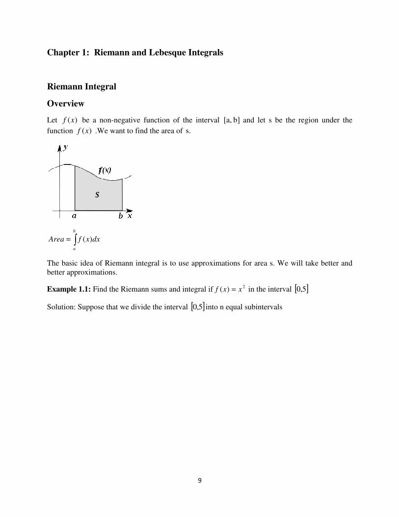
Let )(xf be a non-negative function of the interval
function )(xf .We want to find the area of
∫=b
a
dxxfArea )(
The basic idea of Riemann integ
better approximations.
Example 1.1: Find the Riemann sums and integral if
Solution: Suppose that we divide the interval
9
Riemann and Lebesque Integrals
negative function of the interval b] [a, and let s be the region under the
.We want to find the area of s.
The basic idea of Riemann integral is to use approximations for area s. We will take better and
Find the Riemann sums and integral if 2)( xxf = in the interval [0
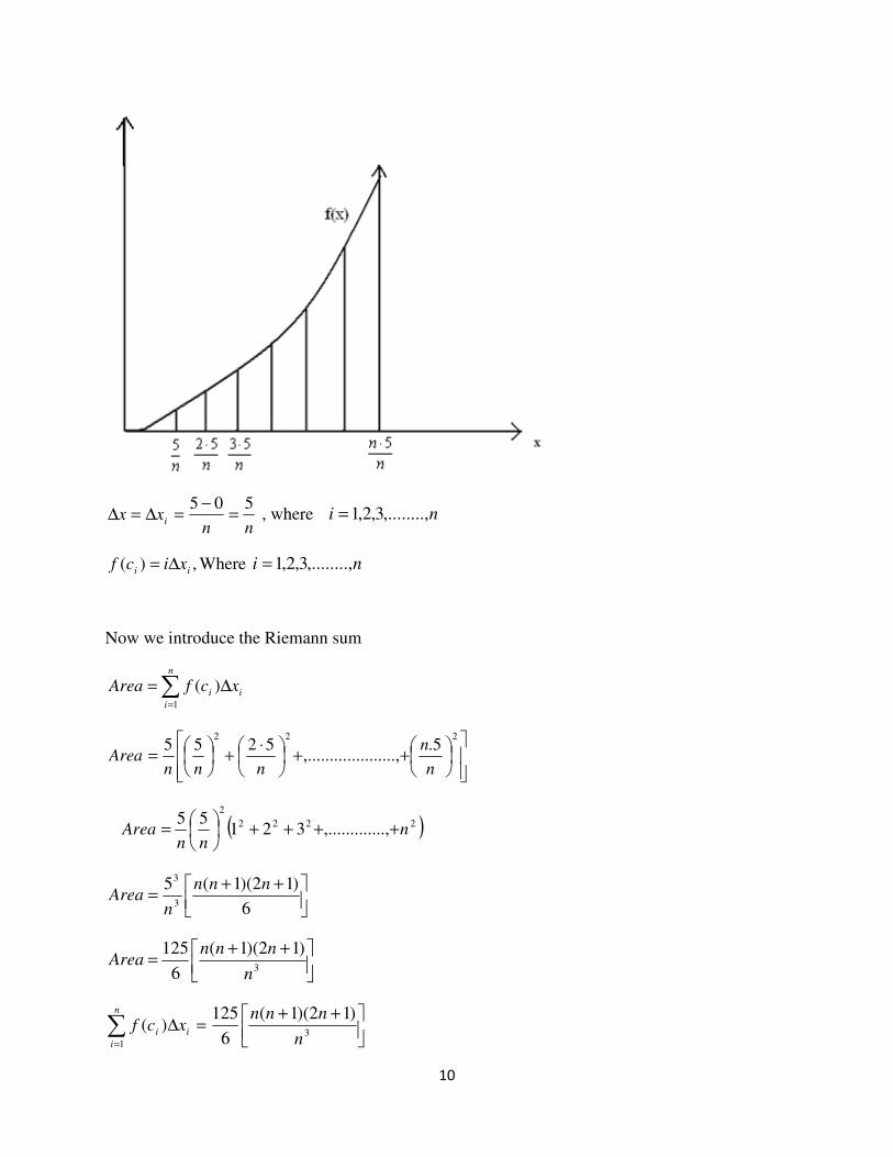
Solution: Suppose that we divide the interval [ ]5,0 into n equal subintervals
and let s be the region under the
ral is to use approximations for area s. We will take better and
]5,0
10
nnxx i
505=
−=∆=∆ , where ni ,........,3,2,1=
,)( ii xicf ∆= Where ni ,........,3,2,1=
Now we introduce the Riemann sum
i
n
i
i xcfArea ∆=∑=
)(1
++
⋅+
=
2225.
.,..........,.........5255
n
n
nnnArea
( )2222
2
....,,.........32155
nnn
Area ++++
=
++=
6
)12)(1(53
3nnn
nArea
++=
3
)12)(1(
6
125
n
nnnArea
=∆∑=
i
n
i
i xcf )(1
++3
)12)(1(
6
125
n
nnn
11
This is a Riemann sums
Now we introduce the Riemann integral
i
n
i
in
xcf ∆∑=
∞→)(lim
1
=∆∑=
∞→i
n
i
in
xcf )(lim1
++
∞→ 3
)12)(1(lim
6
125
n
nnn
n
∫ =b
a
dxxf3
125)(
Example 1.2: 2)( xxf = in the interval [ ]5,0
Suppose that we divide the interval [ ]5,0 into five rectangles
From the above example we know that
=∆∑=
i
n
i
i xcf )(1
++3
)12)(1(
6
125
n
nnn
So we take 5=n
55)(5
1
=∆= ∑=
i
i
i xcfArea
∫ ==5
0
2666.41dxxArea
100)( ⋅−= eapproximatActualError Percent
333.13=Error Percent
Now if we divide the interval [ ]5,0 into 10 rectangles then
++=∆∑
=3
1
)12)(1(
6
125)(
n
nnnxcf i
n
i
i
So we will take 10=n
∫ =b
a
dxxf )(
12
125.48)(10
1
=∆= ∑=
i
i
i xcfArea
100)( ⋅−= eapproximatActualError Percent
4584.6=Error Percent
According to the above example which explains the idea of Riemann sums, we observe that
when the area becomes smaller and smaller we will get better condition of approximation.
13
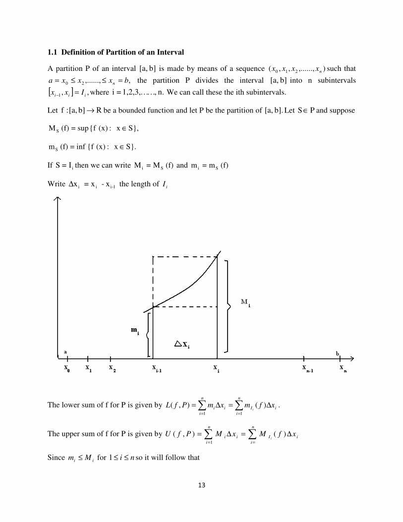
1.1 Definition of Partition of an Interval
A partition P of an interval b] [a, is made by means of a sequence ),......,,,( 210 nxxxx such that
,,......,20 bxxxa n =≤≤= the partition P divides the interval b] [a, into n subintervals
[ ] ,,1 iii Ixx =− where n. ,……1,2,3,=i We can call these the ith subintervals.
Let Rb] [a, :f → be a bounded function and let P be the partition of b]. [a, Let PS∈ and suppose
S}, x:(x) {f sup=(f) MS ∈
S}. x:(x) {f inf=(f) mS ∈
If iI=S then we can write (f) M=M Si and (f) m=m Si
Write x- x= x 1-iii∆ the length of iI
The lower sum of f for P is given by i
n
i
I
n
i
ii xfmxmPfLi
∆=∆= ∑∑==
)(),(11
.
The upper sum of f for P is given by i
n
i
Ii
n
i
i xfMxMPfUi
∆=∆= ∑∑==
)(),(1
Since ii Mm ≤ for ni ≤≤1 so it will follow that
14
),(),( PfUPfL ≤ for all bounded f and for all partitions P.
We approximate the area under the curve by choosing the partitions P progressively finer.
Definition
A partition 1P is called refines of a partition P if every point of P is a point in 1P .
Example if ( )5,4,3,2,1,01 =P and )5,3,2,0(=P then 1P is called refines of P
Theorem1.1: If 1P refines P then ).,(),(),(),( 11 PfUPfUPfLPfL ≤≤≤
From this theorem follows that ),(inf),(sup PfUPfL Pp ≤ )2(
Where the inf and sup are taken over all partitions P
Definition: A function [ ] Rbaf →,: is a Riemann integrable if the inequality of equation (2) is
valid for .f Now we are coming to the proper definition of Riemann sums and the integral.
1.2 Definition of Riemann Integral
Consider a continuous function f(x) between x=a and x=b , we want to divide the closed interval
[a, b] into n intervals.
Let ax =0 and bxn = definen
abxi
−=∆ and iii xxx −=∆ +1 for ,,,.........3,2,1 ni = this is the
partition of interval [ ]ba, into n subintervals [ ]1, +ii xx each with length .x∆
1
0
1, )( +=
+ ∆=∑ i
n
i
iuppern xxfS
i
n
i
ilowern xxfS ∆=∑=
)(0
,
uppern
b
a
lowern SdxxfS ,, )( ≤≤ ∫
i
n
i
i
b
an
xxfdxxf ∆= ∑∫=
∞→)(lim)(
0
15
1.3 Definition of Sigma-Algebra
Suppose X is a nonempty set and F is a the power set of a set X then F is called sigma-algebra
if it has the following properties
1 F contains the set X as an element
2 If E is a subset of F then complement of E is also a subset of F.
3 The union of countable sets in F is also in F.
Example 1.3: }3,2,1{=X
{ }}3,2,1{},3,2{},3,1{},2,1{},3{},2{},1{,φ=F
FX ∈ F∈}1{ F∈⇒ }2,1{
F∈=∪ }3,2,1{}3,2{}3,2,1{
1.4 Definition of a Measureable Set
A measure m is a function defined on sigma-algebra F over a set X and taking values in the
closed interval [ ]∞,0 such that the following properties are satisfied.
1 0)( =φm
2 If ,.........,, 321 EEE is a countable sequence of pair wise disjoint sets in F then
3 )()(11
∑∞
=
∞
=
=i
i
i
i EmEm U .
Then (X, F, m) is called measureable space and the members of F are called measureable sets.
1.5 Definition of Lebesque Integral
A new method was presented by Lebesque in 1902, as a new approach to the domain of the
function in comparison the Riemann integral. He chose to make partition of the range. Thus, for
each interval in the partition, rather than asking for the value of the function between the end
points in the x-axis, we asked how much of the domain is mapped by the function to some value
between two end points of the y-axis. In the Lebesque integral define we consider the closed
interval [c, d] and the partition P of ranges such that nyyyy ≤≤≤≤ ..........210 .Let cy =0 and
dyn = define as n
cdy
−=∆ and 1−−=∆ iii yyy so the upper and the lower sums will be defined
as
{ }ii
n
i
i yxfyxmyPfL <≤∆= −=
∑ )(:(),( 1
1
16
{ }ii
n
i
i yxfyxmyPfU ≤<∆= −=
∑ )(:(),( 1
1
),(),( PfUPfL ≤
∫ ≤≤E
PfUdxxfPfL ),()(),(
{ }))((lim)(1
iii
n
i
in
E
yxfymydxxf ≤≤= −=
∞→∑∫
1.6 Characteristic and Simple Function [15]
Let us consider any set A. The function
is called characteristic function of A .A finite linear combination of characteristic functions
)()( xXaxsiEi∑=
is simple function if all sets iE are measurable.
1.7 Definition of Lebesque Integral for a Simple Function [15]
If )()( xXaxsnAn∑= is simple function )( nAm and is finite for all n, then the Lebesque integral
of s is defined as
)()( nn Amadxxs∫ ∑=
If E is a measurable set then we define
dxxsxXdxxsE
E )()()(∫ ∫=
Example1.4: If 2)( =xf over the closed interval [ ]3,2 the constant function can be written as a
simple function
).(2)( xXxf R=
17
Then the Lebesque integral over [ ]3,2 will be
[ ]
[ ] dxxXdxxf )(2)( 3,2
3,2
∫∫ =
[ ])3,2(2m=
)23(2 −=
Theorem: If f is bounded on [a, b] such that f is Riemann integrable then it is Lebesque
integrable on [a, b] but the reverse is not always true
Example1.5: Consider a Dirichlet function
Then g (x) is Lebesque integrable but not Riemann integrable because
Let us consider a partition 1.,,.........0: 210 =<<<= nxxxxP of interval [ ]1,0 .Then it is easy to
check that
SUP of 1)( =xf [ ]ii xxx ,1−∈ and inf of 0)( =xf [ ]ii xxx 1−∈
Hence the upper and lower Riemann sums of g(x) with respect to P satisfied
1),( =fPU and 0),( =fPL
then )(xg is not Riemann integrable.
1.8 The General Definition of Lebesque Integral
Suppose that f(x) is a measureable function define on both positive and negative parts of ).(xf
Then
).0),(max()( xfxf =+
).0),(max()( xfxf −=−
So we can write
−+ −= fff
Then the Lebesque integral will be
fdxxfE E
()(∫ ∫+=
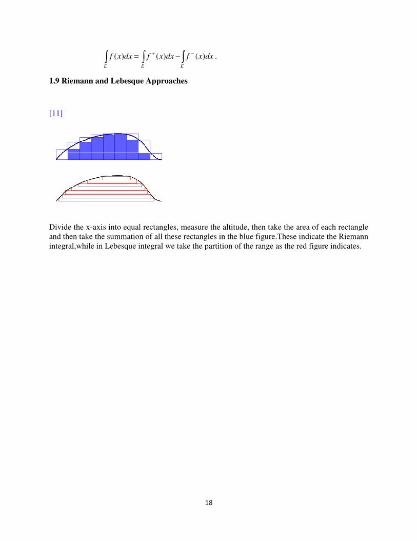
1.9 Riemann and Lebesque Approaches
[11]
Divide the x-axis into equal rectangles, measure the altitude, then take the area of each rectangle
and then take the summation of all these rectangles in the blue figure.These indicate the Riema
integral,while in Lebesque integral we take the partition of the range
18
dxxfdxxE
)()( ∫−− .
pproaches
axis into equal rectangles, measure the altitude, then take the area of each rectangle
and then take the summation of all these rectangles in the blue figure.These indicate the Riema
integral,while in Lebesque integral we take the partition of the range as the red figure indicates.
axis into equal rectangles, measure the altitude, then take the area of each rectangle
and then take the summation of all these rectangles in the blue figure.These indicate the Riemann
as the red figure indicates.
19
Chapter 2: Fuzzy Set
2.1 Fuzzy Sets
If we use the expression ``a set`` then we can say that the collection of well defined distinct
objects is called set. Define d}, c, b, {a, =A since we can count number of elements then A is
called finite set .If we cannot count the number of elements then the set is called an infinite set
for example ..}……7 5, 3, {1,=B
Consider a function {0,1},:A →Xχ which is called a characteristic function of the crisp set A if
and only if ∀ Xx ∈ we have
In fuzzy set theory the classical sets are called crisp sets for the reason that we can differentiate
between fuzzy set and the classical set, in fuzzy set theory the above characteristic function is
converted to a membership function if we assign every Xx ∈ a value from the unit interval
1] [0, instead of the set [ ]21}. {0,
2.2 Definition of a Fuzzy Set
A set { })(,(:),( xxyxA Aµ= , Xx ∈ is called a fuzzy set where )(xAµ is the membership
function of a fuzzy set A and is defined as [ ]1,0: →XAµ , the value of )(xAµ is called the
membership degree of X .
Every element Xx ∈ has thus a membership degree [ ]1,0)( ∈= xy Aµ .
2.3 The Notation for Fuzzy Set
The discrete set is define as
n
nAAA
x
x
x
x
x
xA
)(...,,.........
)()(
2
2
1
1 µµµ+++=
where nxxx ,........,, 21 are members of A
and )(...,),........(),( 21 nAAA xxx µµµ are the membership degrees of nXXXX ,.....,,, 321 .
20
The sign ""+ has a symbolic character as a joint of the set’s elements.
For continuous fuzzy set, a fuzzy set A can be defined as
∫=X
x
xA
)(µ
or
∑∈Xx
A
x
x)(µ
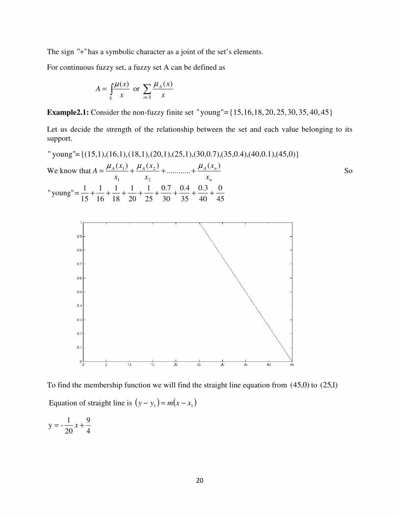
Example2.1: Consider the non-fuzzy finite set 45} 40, 35, 30, 25, 20, 18, 16, {15, = young""
Let us decide the strength of the relationship between the set and each value belonging to its
support.
(45,0)}(40,0.1),(35,0.4),(30,0.7),(25,1),(20,1),1), (18, (16,1),{(15,1), =young" "
We know thatn
nAAA
x
x
x
x
x
xA
)(............
)()(
2
2
1
1 µµµ+++= So
45
0
40
0.3
35
0.4
30
0.7
25
1
20
1
18
1
16
1
15
1 =young"" ++++++++
To find the membership function we will find the straight line equation from )0,45( to )1,25(
Equation of straight line is ( ) ( )11 xxmyy −=−
4
9
20
1-y += x
21
Membership Function
1)("" == xy youngµ if 250 <≤ x and 4
9
20
1-)(y "" +== xxyoungµ if 4525 ≤≤ x
By using the same way, we can also find the memberships for “middle-aged” and “old-aged”
people.
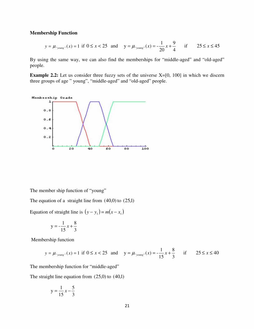
Example 2.2: Let us consider three fuzzy sets of the universe X=[0, 100] in which we discern
three groups of age ” young”, “middle-aged” and “old-aged” people.
The member ship function of “young”
The equation of a straight line from )0,40( to )1,25(
Equation of straight line is ( ) ( )11 xxmyy −=−
3
8
15
1-y += x
Membership function
1)("" == xy youngµ if 250 <≤ x and 3
8
15
1-)(y "" +== xxyoungµ if 4025 ≤≤ x
The membership function for “middle-aged”
The straight line equation from )0,25( to )1,40(
3
5
15
1y −= x

22
3
5
15
1)(y "" −== − xxagedmiddleµ if 4025 ≤≤ x
Similarly we can find 3
13
15
1)(y "" +−== − xxagedmiddleµ if 6550 ≤≤ x
1)(y "" == − xagedmiddleµ if 5040 ≤≤ x
The member ship function for “old-aged” people
The straight line equation from 1) (65, to0) (50,
3
10
15
1y −= x
3
10
15
1)(y "" −== − xxagedoldµ if 65x50 ≤≤ and 65 xif 1=y ≥
2.4 Special Continuous Membership Functions
Now we are introducing the formula for continuous functions, the s-class function ) ,, s(x, γβα
with parameter , and , γβα
γβαγα
β << and 2
= where+
Example 2.3: Now we are using the above formula, draw the graph of the s-function
45= and 25= with γα
The graph of )45,35,25,(Xs will be
23
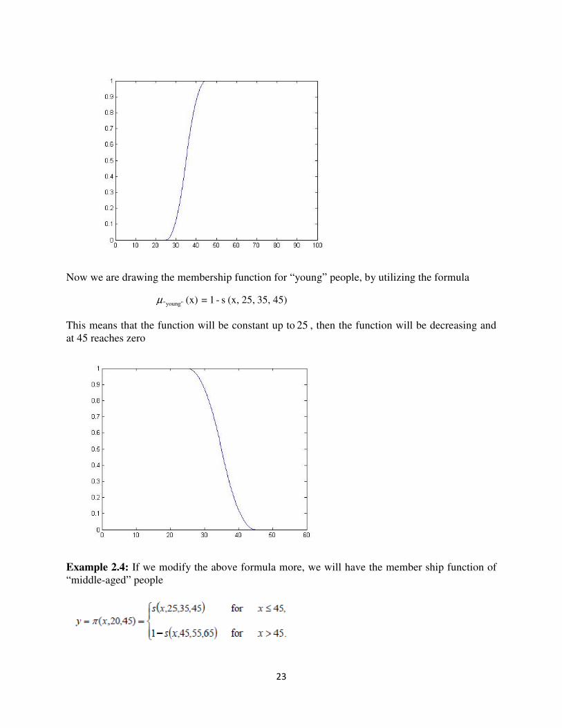
Now we are drawing the membership function for “young” people, by utilizing the formula
45) 35, 25, (x, s -1=(x)young""µ
This means that the function will be constant up to 25 , then the function will be decreasing and
at 45 reaches zero
Example 2.4: If we modify the above formula more, we will have the member ship function of
“middle-aged” people
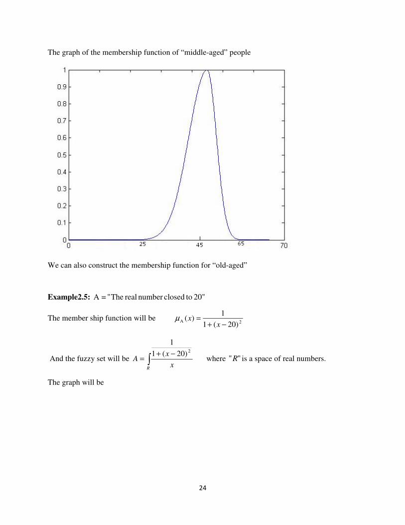
24
The graph of the membership function of “middle-aged” people
We can also construct the membership function for “old-aged”
Example2.5: 20" toclosednumber real The" =A
The member ship function will be 2A
)20(1
1)(
−+=
xxµ
And the fuzzy set will be ∫−+
=R
x
xA
2)20(1
1
where ""R is a space of real numbers.
The graph will be
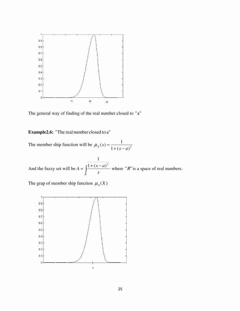
25
The general way of finding of the real number closed to a""
Example2.6: a" toclosednumber real The"
The member ship function will be 2A
)(1
1)(
axx
−+=µ
And the fuzzy set will be ∫−+
=R
x
axA
2)(1
1
where ""R is a space of real numbers.
The grap of member ship function )(XAµ
26
Chapter 3: Fuzzy Measure Choquet and Sugeno Integrals
Fuzzy Measure
3.1 Measure
Measure is one of the most important concepts in mathematics, as well as the i-e,concept of
integration w. r. t a given measure. In the classical definition of measure we use additive
property. Additivity is very effective in many applications, but in many real world problems we
do not require measure with respect to the additive feature, for example in fuzzy logic, artificial
intelligence, data mining, decision making theory etc, a large amount of open problems for
example the efficiency of a set of workers is being measured, we use the definition of non
additive measure.
The fuzzy measure does not require additivity in most cases, in fuzzy measure we require
monotonicity related to inclusion of sets.
3.2 Definition of Fuzzy Measure (Monotonic) [5]
Suppose that ) F, (X, µ is a measureable space, a fuzzy measure is a function ][0,F: ∞→µ such
that the following properties are held
1 0=)(φµ
2 B)((A) then BA and FBA, If µµ ≤⊆∈
3 then..............AAAA and FA If 4321n ⊆⊆⊆∈ )lim()(lim nn
nn
AA∞→∞→
= µµ
3.3 Definition of the Additive Measure
Let us consider m) F, (X, to be a measure space .An additive measure m is a function
][0,F :m ∞→ i-e defined on sigma-algebra F over a set X and taking values in the interval
] [0, ∞ such that the following properties are satisfied
1 0= )( m φ
2 If ..………,E ,E ,E 321 is a countable sequence of pair wise disjoint subsets of F
)m(E=) E( mthen 1i
i
1i
i ∑∞
=
∞
=
U
Example of additive measure is a well known example of Lebesque measures, he generalize the
concept of length of a segment.
3.4 Sugeno Fuzzy Measure [5]
A Sugeno fuzzy measure is a function [0,1]F: →µ such that
27
1 0)( =φµ
2 If BA ⊆ then )()( BA µµ ≤ , then..............AAAA and FA If 4321n ⊆⊆⊆∈
)lim()(lim nn
nn
AA∞→∞→
= µµ
3.5 Definition of Possibility Measure (Zedeh, 1978)
Let m) F, (X, be a measureable space .A possibility measure is a function [0,1]F :m →
,satisfying the following condition
1 0= )( m φ
2 1=m(X)
3 m(B) m(A) then BA If ≤⊆
4 { })(sup)( iIi
Ii
i AmAm ∈
∈
=U
Definition of conormst − or normss −
conormst − or normss − are associative, commutative, and monotonic two-placed functions s
that map from [ ] [ ]1,01,0 × into [ ]1,0 .These properties are formulated with the following
conditions:
1. 1)1,1( =s ; ),())(,0()0),(( XXsXsAAA
µµµ == Xx ∈
2. ))((),(())((),(( XsXsXsXsDCBA
µµµµ ≤ if )(()(( XsXsCA
µµ ≤
and )(()(( XsXsDB
µµ ≤
3. ))(()(())(()(( XsXsXsXsABBA
µµµµ ≤=≤
4. ))(()),((),((())(((),(((),(( XXXsXsXsXsCBACBA
µµµµµµ =
3.6 Definition of s-Decomposable Measure (Weber 1984)
Weber defined the s-Decomposable measure by giving a general concept of fuzzy -λ measure
and the possibility measures.
Suppose that s is a t-conorm then for any measureable space m), F, (X, a ledecomposab-s
measure is a function [0,1]F :m → such that
1 0= )( m φ
2 1=m(X)
3 For all disjoint subsets m(B))S(m(A),=m(AUB) F,BA, ∈
3.7 Definition of Sugeno λ -Fuzzy Measure
Let }x………,x,x,{x =X n321 be a finite set and consider ),(-1,∞∈λ an λ -measure is a
function [0,1]2:gX →λ such that it satisfied the following condition
28
1 1=(X)g λ
2 φλ λλλλλ =BA with (B)(A)gg +(B) g +(A) g =B) (A Ug then 2BA, If X ∩∈
Moreover, let X be a finite set, { }nxxxX .,,........., 21= and )(XP be the class of all subsets of X
the fuzzy measure ()( λgXg = { }).,,........., 21 nxxx can be formulated as (Leszczyński et al.,
1985)
(λg { }).,,........., 21 nxxx =n
n
i
n
i
n
ii
i
n
i
i gggggg ................ 21
11
1 112
1 12
1
−−
= +==
+++ ∑ ∑∑ λλ
=
−+∏
=
n
i
ig1
1)1(1
λλ
where ),1( ∞−∈λ
(λg { } λ).,,........., 21 nxxx =∏=
−+n
i
ig1
1)1( λ
(λg { } 1).,,........., 21 +λnxxx =∏=
n
i 1
)1( igλ+ by definition (λg { } 1).,,........., 21 =nxxx
And ( )∏=
+n
1i
i 1g=1+ λλ
Now we evaluate the value of λ
According to the fundamental theorem regarding the λ-fuzzy measure (Leszczyński et al., 1985),
λ -value has three cases, as follows:
(i) 0. < < 1- then g(X)> g Ifn
1i
i λ∑=
(ii) 0. = then g(X)= g Ifn
1i
i λ∑=
(iii) 0. then g(X) g Ifn
1i
i ><∑=
λ
3.8 Definition (Discrete Case)
A fuzzy measure µ on finite set X is a function [0,1]2: X →µ satisfying the following axioms
1 0)( =φµ
2 (B)(A) then BA If µµ ≤⊆
3 1)( =Xµ
29
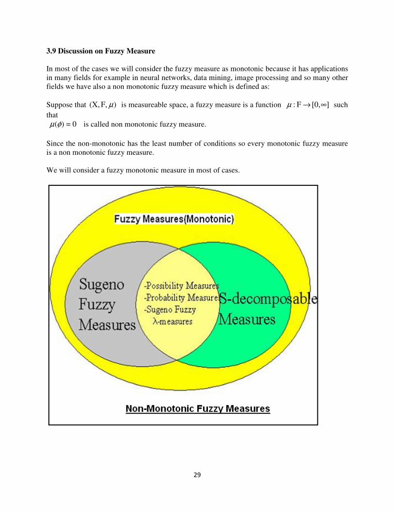
3.9 Discussion on Fuzzy Measure
In most of the cases we will consider the fuzzy measure as monotonic because it has applications
in many fields for example in neural networks, data mining, image processing and so many other
fields we have also a non monotonic fuzzy measure which is defined as:
Suppose that ) F, (X, µ is measureable space, a fuzzy measure is a function ][0,F: ∞→µ such
that
0=)(φµ is called non monotonic fuzzy measure.
Since the non-monotonic has the least number of conditions so every monotonic fuzzy measure
is a non monotonic fuzzy measure.
We will consider a fuzzy monotonic measure in most of cases.
30
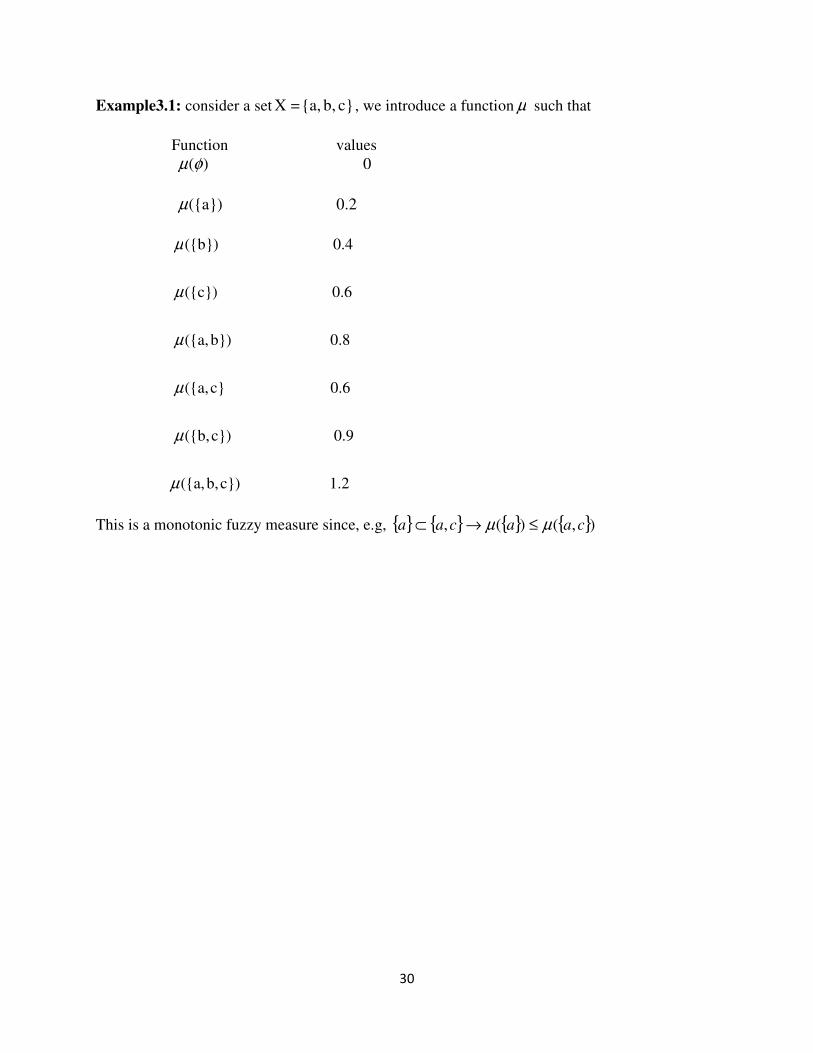
Example3.1: consider a set c} b, {a, =X , we introduce a function µ such that
Function values
0 )(φµ
0.2 ({a}) µ
1.2 c})b,({a,
0.9 c})({b,
0.6 c}({a,
0.8 b})({a,
0.6 ({c})
0.4 ({b})
µ
µ
µ
µ
µ
µ
This is a monotonic fuzzy measure since, e.g, { } { } { } { }),()(, caacaa µµ ≤→⊂
31
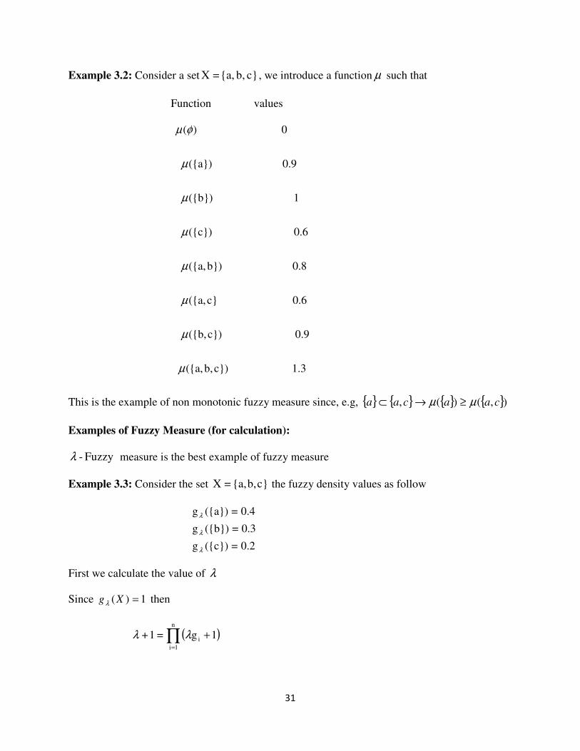
Example 3.2: Consider a set c} b, {a, =X , we introduce a function µ such that
Function values
1.3 c})b,({a,
0.9 c})({b,
0.6 c}({a,
0.8 b})({a,
0.6 ({c})
1 ({b})
0.9 ({a})
0 )(
µ
µ
µ
µ
µ
µ
µ
φµ
This is the example of non monotonic fuzzy measure since, e.g, { } { } { } { }),()(, caacaa µµ ≥→⊂
Examples of Fuzzy Measure (for calculation):
Fuzzy -λ measure is the best example of fuzzy measure
Example 3.3: Consider the set c}b,{a,=X the fuzzy density values as follow
0.2=({c})g
0.3=({b})g
0.4=({a})g
λ
λ
λ
First we calculate the value of λ
Since 1)( =Xgλ then
( )∏=
+n
1i
i 1g=1+ λλ
32
1)+1)(0.2+1)(0.3+(0.4=1+ λλλλ
0=0.1 -0.26+0.024 23 λλλ
The roots of the above equation will be
} 0.3719 {0,-11.87, =λ
But )(-1,∞∈λ
So we will take 0.3719 =λ
For g 0 =λ is additive measure
If 0.3719 =λ then
0.2=({c}) g
0.3=({b}) g
0.4=({a}) g
λ
λ
λ
0.6298=({c}) g ({a}) g+({c}) g +({a}) g =c})({a, g
0.7446=({b}) g ({a}) g+({b}) g +({a}) g =b})({a, g
λλλλλ
λλλλλ
λ
λ
0.5223=({c}) g ({b}) g +({c}) g +({b}) g =c})({b, g λλλλλ λ
1=(X) gλ
For 0.3719 =λ this is fuzzy measure because for example
(X) g b}{a, g then Xb}{a, If
b}{a, g {a} g then b}{a,{a} If
≤⊆
≤⊆
Similarly we can take all other cases
33
Example3.4: Calculation of λ -fuzzy measure for set the students in bth of complex analysis.
Let X= {a(those students who got 5 grade in complex analysis), b(those students who got 4 grade
in complex analysis), c= (those students who got 3 grade in complex analysis)}
Solution Let the associated densities are
0.5=({a})gg1 λ=
0.4=({b}gg 2 λ=
0.3=({c})gg3 λ=
First we calculate the value of λ
We know that
( )∏=
+n
1i
i 1g=1+ λλ
1)+1)(0.3+1)(0.4+(0.5=1+ λλλλ
0=0.20.47+0.06 23 λλλ +
And the roots of the above equation will be
} 0.4335- 5,{0,-23.066 =λ
But ),1( ∞−∈λ
So we will take 4335.0−=λ
If 0=λ then the measure is additive measure
If 4335.0−=λ then
0.3=({c}) g
0.4=({b}) g
0.5=({a}) g
λ
λ
λ
34
0.7350=({c}) g ({a}) g+({c}) g +({a}) g =c})({a, g
0.8133=({b}) g ({a}) g+({b}) g +({a}) g =b})({a, g
λλλλλ
λλλλλ
λ
λ
0.6480=({c}) g ({b}) g +({c}) g +({b}) g =c})({b, g λλλλλ λ
1=(X) gλ
For 4335.0−=λ the above problem represent a fuzzy measure
3.10 Definition of Choquet Integral
Let us suppose that � be a fuzzy measure on X , then Choquet integral of a function
] [0,X:f ∞→ w.r.t fuzzy measure g is defined
( ) )()()(dg f(c)1
1 i
n
i
ii Agxfxf∑∫=
−−= where XAi ⊂ for ni ,.....,3,2,1=
where )}f(x..,…),f(x, )f(x ),f(x { n321 are the ranges and they are defined as
where )f(x..…)f(x )f(x )f(x n321 ≤≤≤≤ and 0)( 0 =xf
( ) )()()(dg f(c)1
1 i
n
i
ii Agxfxf∑∫=
−−= is an equation is called Choquet integral.
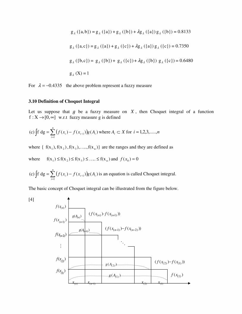
The basic concept of Choquet integral can be illustrated from the figure below.
[4]
( 1)( )ng A −
)(nx )1( −nx
)2(x )1(x
( 2)( )nf x −
OM
(1)( )g A
(2)( )g A
( ) ( -1)( ( )- ( ))n nf x f x
(1)( )f x
(2) (1)( ( ) ( ))f x f x−
( 1) ( 2)( ( ) ( ))n nf x f x− −−
( )( )ng A
( )( )nf x
( 1)( )
nf x
−
(2)( )f x
(1)( )f x
35
Explanation of Choquet Integral w.r.t figure above
Let }x..,…,x, x, x{ =X n321 be n objects with ranges )}f(x..,…),f(x, )f(x ),f(x { n321 such
that )f(x..…)f(x )f(x )f(x n321 ≤≤≤≤
Now the measurements of these objects are )( 1Ag )( 2Ag ................. )( nAg
The area of first rectangle )( 1xf= ⋅ )( 1Ag where { }( )nxxxxgAg ,......,,)( 3211 =
The area of second rectangle ( ) )()()( 212 Agxfxf ⋅−= where { }( )nxxxgAg ,......,)( 322 =
The area of third rectangle ( ) )()()( 323 Agxfxf ⋅−= where { }( )nxxxgAg ,......,)( 433 =
The area of nth rectangle ( ) )()()( 1 nnn Agxfxf ⋅−= − where { }( )nn xgAg =)(
The sum of these areas will be
)()( 1xffdgc =∫ ⋅ )( 1Ag ( ) )()()( 212 Agxfxf ⋅−+ ( ) +⋅−+ )()()( 212 Agxfxf
( ) )()()(.............. 1 nnn Agxfxf ⋅−+ −
( ) )()()(dg f(c)1
1 i
n
i
ii Agxfxf∑∫=
−−=
36
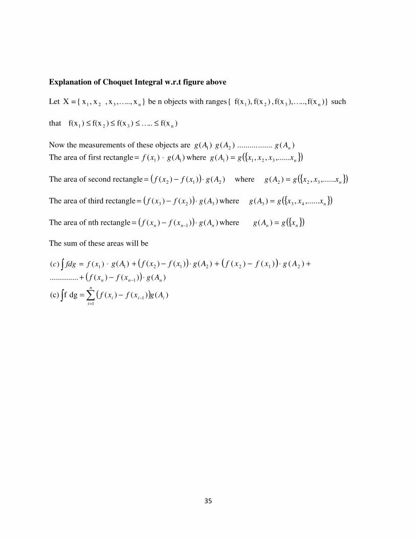
Example3.5: Consider a set }x,x,{x =X 321 where the ranges are defined as
0.5= )(x f 0.3,= )(x f 0.2,= )(x f 221 , such that the fuzzy measure (monotonic) is defined as
Function values
0 )(φµ
0.2 })({x 1µ
1.2 })x,x,({x
0.9 })x,({x
0.6 }x,({x
0.8 })x,({x
0.5 })({x
0.4 })({x
321
31
32
21
3
2
µ
µ
µ
µ
µ
µ
The Choquet integral for this problem is defined as
( ) )()()(d f(c)3
1
1 i
i
ii Axfxf µµ ∑∫=
−−=
)( 1xf= ⋅ { } +),,( 321 xxxµ ( ) { }( ) ( ) { }( )3233212 )((,)(( xxfxfxxxfxf µµ ⋅−+⋅−
37
0.50.3)-(0.5+0.60.2)-(0.3+1.20.2 = ⋅⋅⋅ 4.0d f(c) =∫ µ
This is the Choquet integral for monotonic fuzzy measure
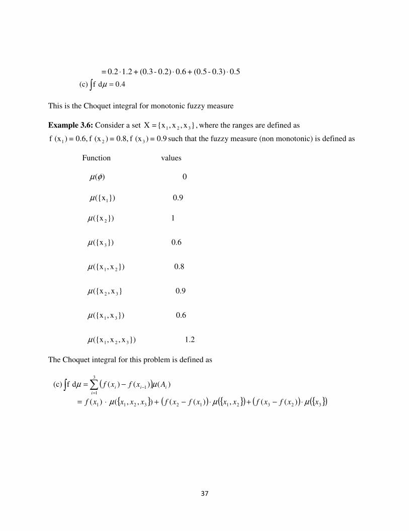
Example 3.6: Consider a set , }x,x,{x =X 321 where the ranges are defined as
0.9= )(x f 0.8,= )(x f 0.6,= )(x f 321 such that the fuzzy measure (non monotonic) is defined as
Function values
0 )(φµ
0.9 })({x 1µ
1.2 })x,x,({x
0.6 })x,({x
0.9 }x,({x
0.8 })x,({x
0.6 })({x
1 })({x
321
31
32
21
3
2
µ
µ
µ
µ
µ
µ
The Choquet integral for this problem is defined as
( ) )()()(d f(c)3
1
1 i
i
ii Axfxf µµ ∑∫=
−−=
)( 1xf= ⋅ { } +),,( 321 xxxµ ( ) { }( ) ( ) { }( )3232112 )((,)(( xxfxfxxxfxf µµ ⋅−+⋅−
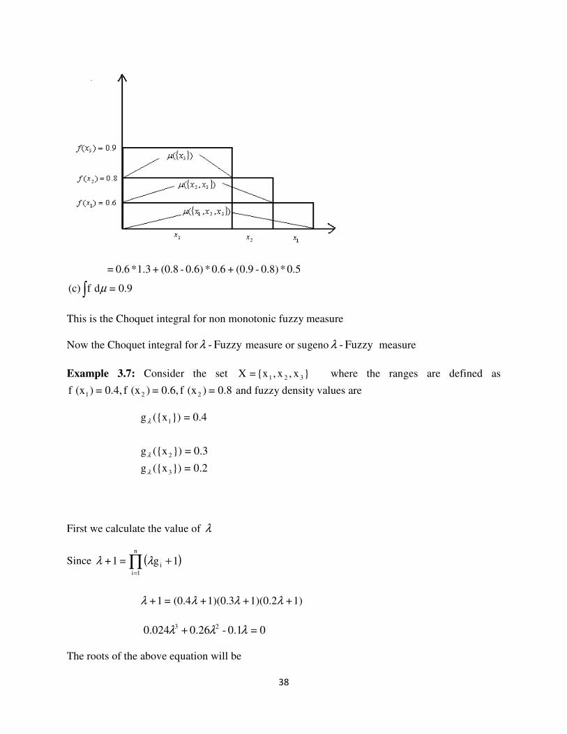
38
0.9= d f(c)
0.5*0.8)-(0.9+0.6*0.6)-(0.8+1.3*0.6 =
∫ µ
This is the Choquet integral for non monotonic fuzzy measure
Now the Choquet integral for Fuzzy-λ measure or sugeno Fuzzy-λ measure
Example 3.7: Consider the set }x,x,{x =X 321 where the ranges are defined as
0.8= )(x f 0.6,= )(x f 0.4,= )(x f 221 and fuzzy density values are
0.2=})({xg
0.3=})({xg
0.4=})({xg
3
2
1
λ
λ
λ
First we calculate the value of λ
Since ( )∏=
+n
1i
i 1g=1+ λλ
1)+1)(0.2+1)(0.3+(0.4=1+ λλλλ
0=0.1-0.26+0.024 23 λλλ
The roots of the above equation will be
39
} 0.3719 {0,-11.87, =λ
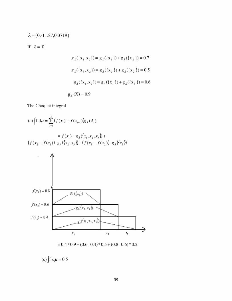
If 0 =λ
= })x,({x 21λg 0.7}) ({xg +}) ({xg 21 =λλ
= })x,({x 23λg 0.5}) ({xg +}) ({xg 23 =λλ
= })x,({x 31λg 0.6}) ({xg +}) ({xg 31 =λλ
0.9=(X) gλ
The Choquet integral
( ) )()()(d f(c)3
1
1 i
i
ii Agxfxf λµ ∑∫=
−−=
)( 1xf= ⋅ { } +),,( 321 xxxgλ
( ) { }( ) ( ) { }( )3233212 )((,)(( xgxfxfxxgxfxf λλ ⋅−+⋅−
0.5= d f(c)
0.2*0.6)-(0.8+0.5*0.4)-(0.6 +0.9*0.4 =
∫ µ
40
then0.3719 = If λ If
0.4}) ({xg 1 =λ
0.3}) ({xg 2 =λ
0.4}) ({xg 1 =λ
= })x,({x 21λg 0.7446=}) ({x})g ({xg}) ({xg +}) ({xg 2121 λλλλ λ+
= })x,({x 32λg 0.5223=}) ({x})g ({xg}) ({xg +}) ({xg 2323 λλλλ λ+
= })x,({x 31λg 0.7323=}) ({x})g ({xg}) ({xg +}) ({xg 3131 λλλλ λ+
1=(X) g λ
The Choquet integral will be
( ) )()()(d f(c)3
1
1 i
i
ii Agxfxf λµ ∑∫=
−−=
)( 1xf= ⋅ { } +),,( 321 xxxgλ ( ) { }( ) ( ) { }( )3233212 )((,)(( xgxfxfxxgxfxf λλ ⋅−+−
0.5445= d f(c)
0.2*0.6)-(0.8+0.5223*0.4)-(0.6 +1*0.4 =
∫ µ
41
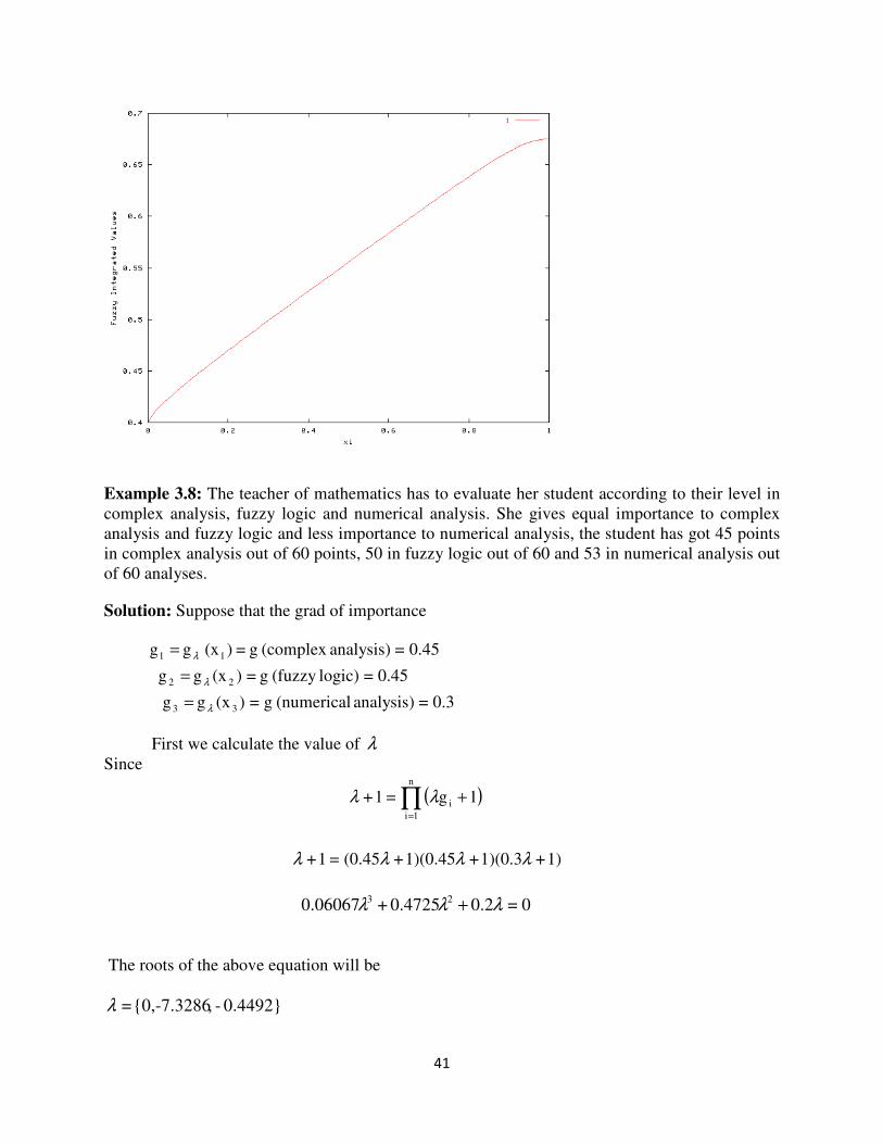
Example 3.8: The teacher of mathematics has to evaluate her student according to their level in
complex analysis, fuzzy logic and numerical analysis. She gives equal importance to complex
analysis and fuzzy logic and less importance to numerical analysis, the student has got 45 points
in complex analysis out of 60 points, 50 in fuzzy logic out of 60 and 53 in numerical analysis out
of 60 analyses.
Solution: Suppose that the grad of importance
0.3=analysis) (numerical g=)(xg g
0.45=logic)(fuzzy g =)(xg g
0.45=analysis)(complex g = )(x g g
33
22
11
λ
λ
λ
=
=
=
First we calculate the value of λ
Since
( )∏=
+n
1i
i 1g=1+ λλ
1)+1)(0.3+1)(0.45+(0.45=1+ λλλλ
0=0.20.4725+0.06067 23 λλλ +
The roots of the above equation will be
} 0.4492- ,{0,-7.3286 =λ
42
But ),1( ∞−∈λ
So we will take 4492.0−=λ
If 0=λ then the measure is additive measure
If 4492.0−=λ then
0.3=})({x g
0.45=})({x g
0.45=})({x g
3
2
1
λ
λ
λ
0.6894=})({x g })({x g+})({x g +})({x g =})x,({x g
0.8090=})({x g })({x g+})({x g +})({x g =})x,({x g
313131
211121
λλλλλ
λλλλλ
λ
λ
0.6894=})({x g })({x g +})({x g +})({x g =})x,({x g 323232 λλλλλ λ
1=(X) gλ
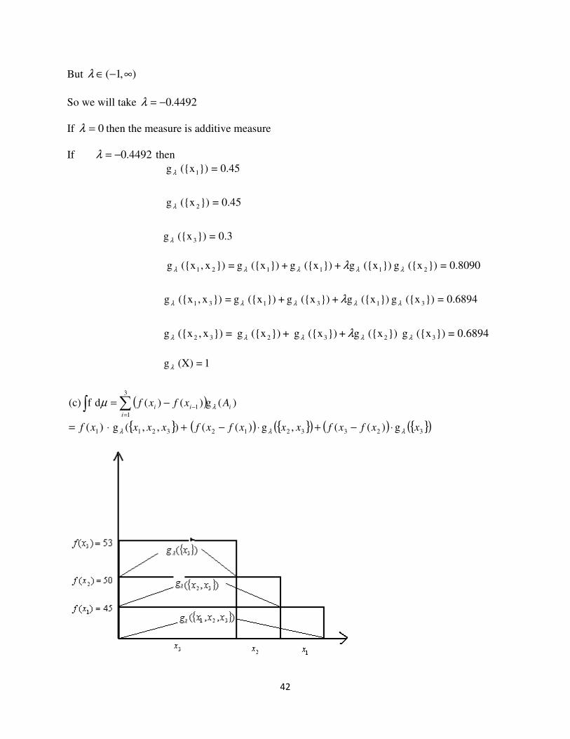
( ) )(g)()(d f(c)3
1
1 i
i
ii Axfxf λµ ∑∫=
−−=
)( 1xf= ⋅ { } +),,(g 321 xxxλ ( ) { }( ) ( ) { }( )3233212 g)((,g)(( xxfxfxxxfxf λλ ⋅−+⋅−
43
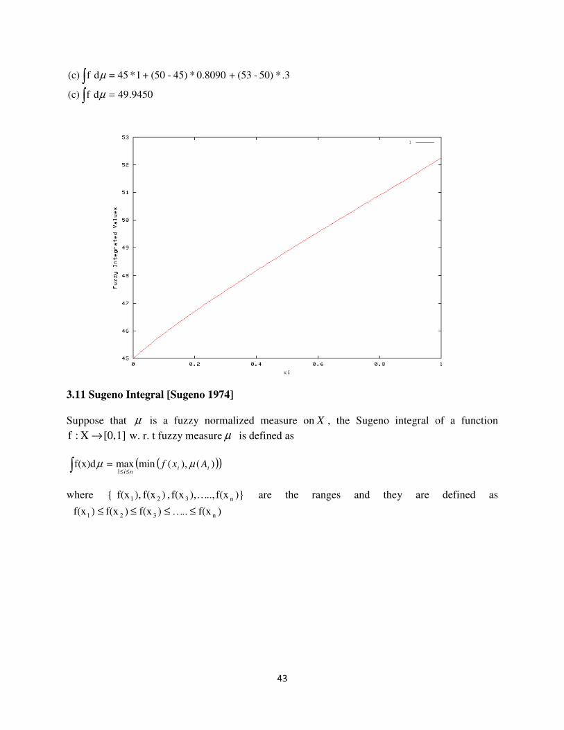
.3*50)-(53+0.8090*45)-(50 +1*45 = d f(c)∫ µ
9450.49d f(c) =∫ µ
3.11 Sugeno Integral [Sugeno 1974]
Suppose that µ is a fuzzy normalized measure on X , the Sugeno integral of a function
1] [0, X:f → w. r. t fuzzy measure µ is defined as
∫ µf(x)d ( )( ))(),(minmax1
iini
Axf µ≤≤
=
where )}f(x..,…),f(x, )f(x ),f(x { n321 are the ranges and they are defined as
)f(x..…)f(x )f(x )f(x n321 ≤≤≤≤
44
Example3.9: Consider a set }x,x,{x =X 321 and the ranges are defined as
0.5= )(x f 0.3,= )(x f 0.2,= )(x f 321 , such that the fuzzy measure (monotonic) is defined as
Function values
0 )(φµ
0.2 })({x 1µ
1.2 })x,x,({x
0.9 })x,({x
0.6 }x,({x
0.8 })x,({x
0.5 })({x
0.4 })({x
321
31
32
21
3
2
µ
µ
µ
µ
µ
µ
To normalize the fuzzy measures, we are dividing all of them by the largest value in measure.
Function values
0 )(φµ
0.16667 })({x 1µ
1 })x,x,({x
0.75 })x,({x
0.5 }x,({x
0.6667 })x,({x
0.416666 })({x
0.333333 })({x
321
31
32
21
3
2
µ
µ
µ
µ
µ
µ
45
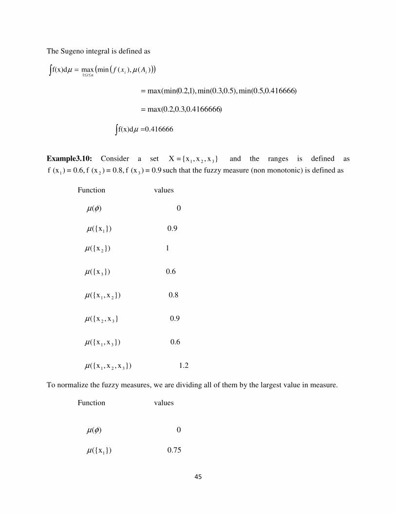
The Sugeno integral is defined as
∫ =µf(x)d ( )( ))(),(minmax1
iini
Axf µ≤≤
)416666.0,5.0min(),5.0,3.0min(),1,2.0max(min(=
)4166666.0,3.0,2.0max(=
416666.0f(x)d∫ =µ
Example3.10: Consider a set }x,x,{x =X 321 and the ranges is defined as
0.9= )(x f 0.8,= )(x f 0.6,= )(x f 321 such that the fuzzy measure (non monotonic) is defined as
Function values
0 )(φµ
0.9 })({x 1µ
1.2 })x,x,({x
0.6 })x,({x
0.9 }x,({x
0.8 })x,({x
0.6 })({x
1 })({x
321
31
32
21
3
2
µ
µ
µ
µ
µ
µ
To normalize the fuzzy measures, we are dividing all of them by the largest value in measure.
Function values
0 )(φµ
0.75 })({x 1µ
46
1 })x,x,({x
0.5 })x,({x
0.8333 }x,({x
0.66667 })x,({x
0.5 })({x
.83333 })({x
321
31
32
21
3
2
µ
µ
µ
µ
µ
µ
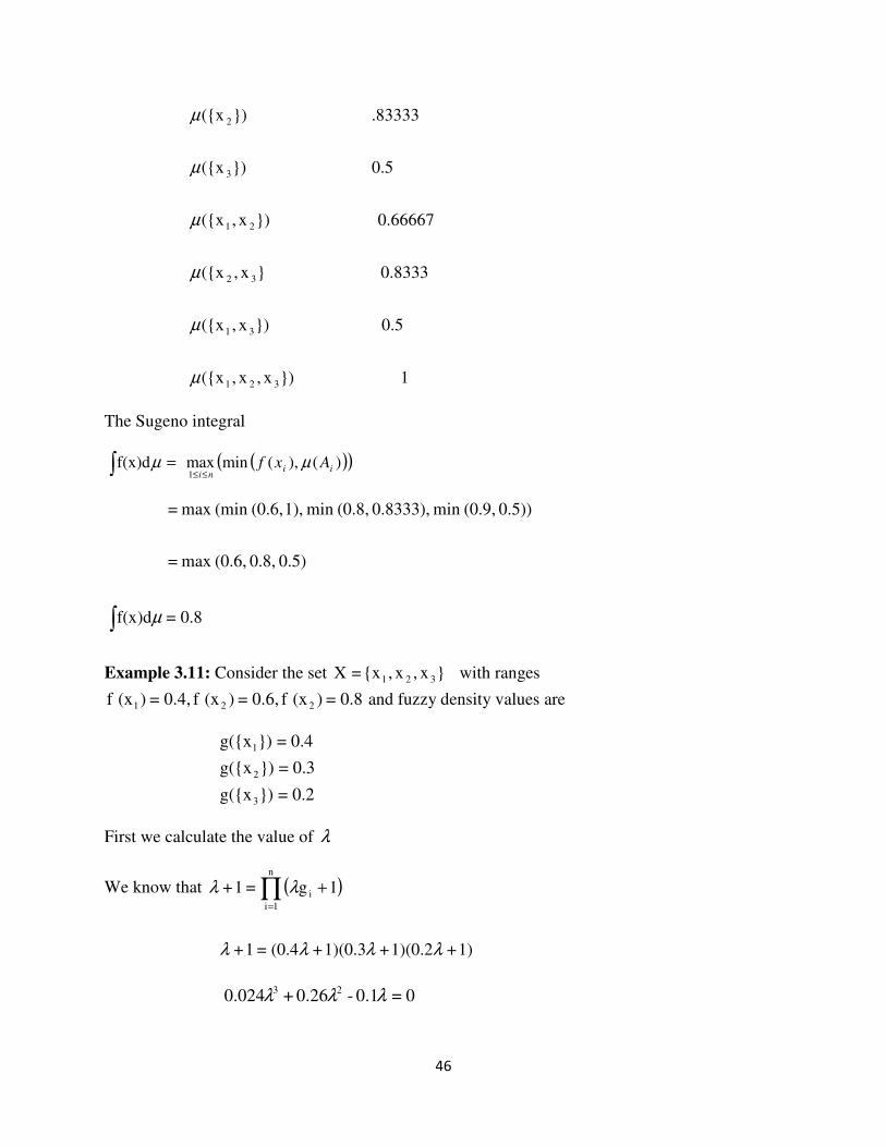
The Sugeno integral
∫ =µf(x)d ( )( ))(),(minmax1
iini
Axf µ≤≤
0.8= f(x)d
0.5) 0.8, (0.6,max =
0.5)) (0.9,min 0.8333), (0.8,min 1), (0.6,(min max =
∫ µ
Example 3.11: Consider the set }x,x,{x =X 321 with ranges
0.8= )(x f 0.6,= )(x f 0.4,= )(x f 221 and fuzzy density values are
0.2=})g({x
0.3=})g({x
0.4=})g({x
3
2
1
First we calculate the value of λ
We know that ( )∏=
+n
1i
i 1g=1+ λλ
1)+1)(0.2+1)(0.3+(0.4=1+ λλλλ
0=0.1-0.26+0.024 23 λλλ
47
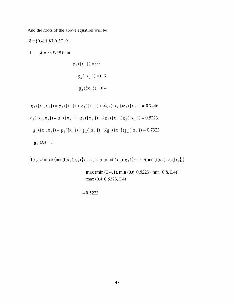
And the roots of the above equation will be
} 0.3719 {0,-11.87, =λ
then0.3719 = If λ
0.4}) ({xg 1 =λ
0.3}) ({xg 2 =λ
0.4}) ({xg 1 =λ
= })x,({x 21λg 0.7446=}) ({x})g ({xg}) ({xg +}) ({xg 2121 λλλλ λ+
= })x,({x 32λg 0.5223=}) ({x})g ({xg}) ({xg +}) ({xg 2323 λλλλ λ+
= })x,({x 31λg 0.7323=}) ({x})g ({xg}) ({xg +}) ({xg 3131 λλλλ λ+
1=(X) g λ
{ } { } { }( ))(),min(f(x),,(),min(f(x(),,,(),min(f(xmaxf(x)d 333223211 xgxxgxxxg λλλµ∫ =
0.5223 =
0.4) 0.5223, (0.4,max =
0.4)) (0.8,min 0.5223), (0.6,min 1), (0.4,(min max =
48
Chapter 4: The Difference between Choquet -Sugeno Integral and Classical
Integrals
4.1 Measure
A measure on X is a non-negative additive set function define on X2 i-e
+→ R2 :f X a normalize measure is called probability measure.
4.2 Signed Measure
A measureable space ( ),, FX that is, a set X with sigma algebra F on it, an extended signed
measure is a function { }−∞∞∪→ ,: RFg such that the following properties are satisfied
1. 0)( =φg
2. ∑∞
=
∞
==
∪
11
)(n
nni
AgAg for any sequence of .,.........,...,,, 321 nAAAA of disjoint sets in .F
A finite signed measure is defined in the same way, but it is only allowed to take )( finite Real
values.
A probability measure is a measure, and a measure is a signed measure
49
4.3 Recall the Definition of Fuzzy Measure [14]
A monotonic fuzzy measure is a function +→ R2 :f X such that it is monotonic and vanishes at
empty set and non monotonic fuzzy measure is a function defines on X2 and vanishes at empty
set.
An additive fuzzy measure is a measure and an additive non monotonic fuzzy measure is signed
measure.
The difference between fuzzy measure and a measure is that, the fuzzy measure is non additive
and additive measures but the measure is additive only this means that every measure is fuzzy
measure but it reverse is not true similarly every signed measure is non monotonic fuzzy
measure but every non monotonic fuzzy measure is not necessarily signed measure.
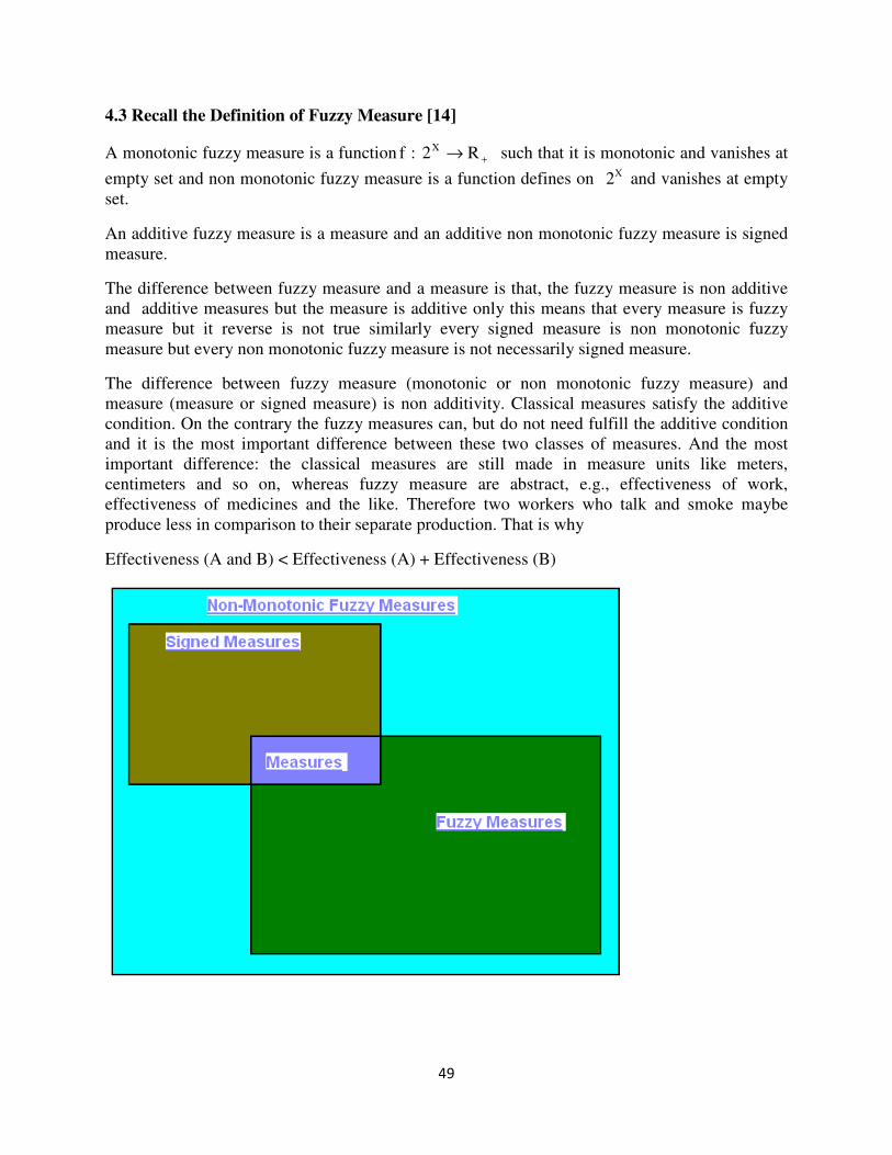
The difference between fuzzy measure (monotonic or non monotonic fuzzy measure) and
measure (measure or signed measure) is non additivity. Classical measures satisfy the additive
condition. On the contrary the fuzzy measures can, but do not need fulfill the additive condition
and it is the most important difference between these two classes of measures. And the most
important difference: the classical measures are still made in measure units like meters,
centimeters and so on, whereas fuzzy measure are abstract, e.g., effectiveness of work,
effectiveness of medicines and the like. Therefore two workers who talk and smoke maybe
produce less in comparison to their separate production. That is why
Effectiveness (A and B) < Effectiveness (A) + Effectiveness (B)
50
Example 4.1: Let φ=∩ BA i.e. A and B are two disjoint sets
Then the measure will be
(B) m+ (A) m = B)(A m ∪
The fuzzy measure will be
( ) )()( BABA µµµ +<∪
OR
( ) )()( BABA µµµ +>∪
( ) )()( BABA µµµ +=∪
To compensate these inequality Sugeno define measurefuzzy -λ which is defined as
( ) )()()()( BABABA µλµµµµ ++=∪ where ),1( ∞−∈λ
4.4 Integration
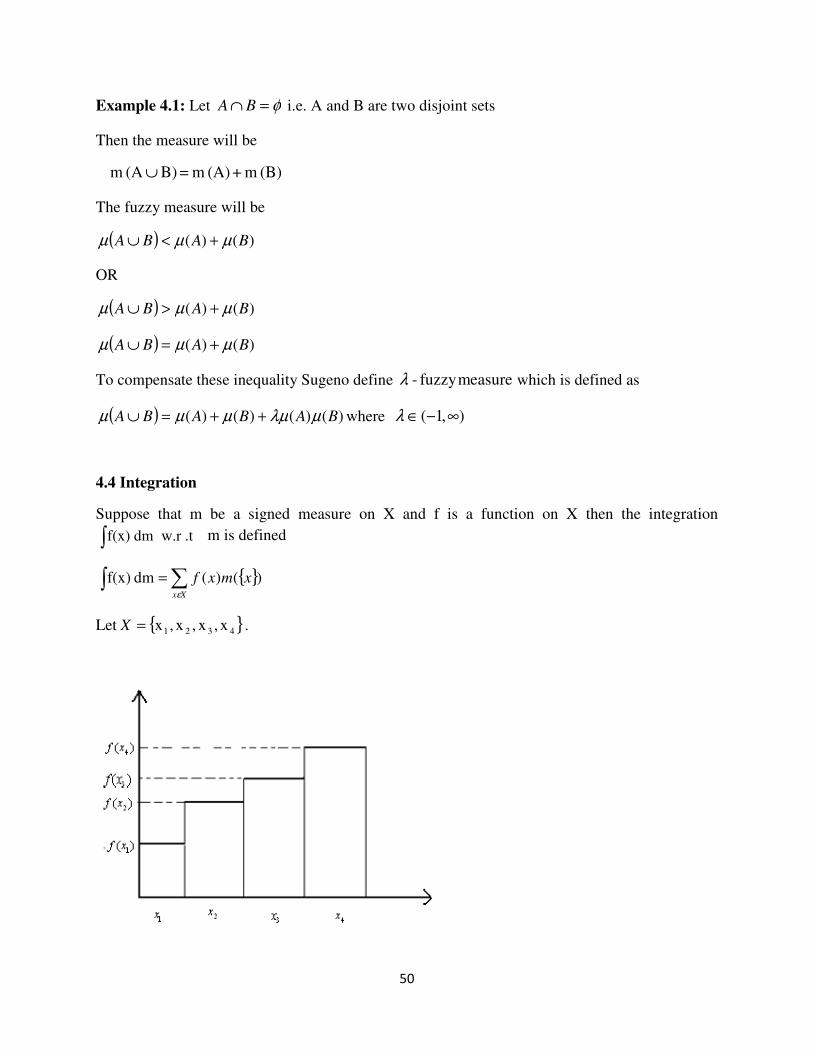
Suppose that m be a signed measure on X and f is a function on X then the integration
.t w.r dm f(x)∫ m is defined
{ })()(dm f(x) ∑∫ =Xx
xmxfε
Let { }4321 x,x,x,x=X .
51
Obviously { } === ∑∫∫ )()(dm f(x))(XxX
xmxfdmxfε
{ } { } { } { })()()()()()()()( 44332211 xmxfxmxfxmxfxmxf +++
Fuzzy integrations (Recall the definition of Choquet and Sugeno integral )
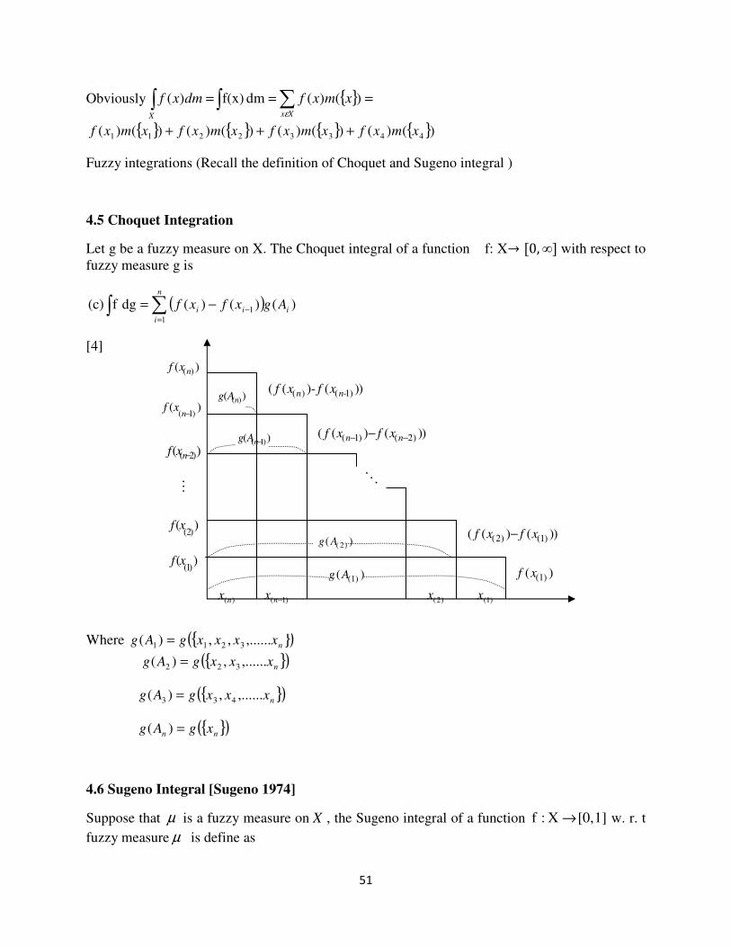
4.5 Choquet Integration
Let g be a fuzzy measure on X. The Choquet integral of a function f: X� �0,∞� with respect to
fuzzy measure g is
( ) )()()(dg f(c)1
1 i
n
i
ii Agxfxf∑∫=
−−=
[4]
Where { }( )nxxxxgAg ,......,,)( 3211 =
{ }( )nxxxgAg ,......,)( 322 =
{ }( )nxxxgAg ,......,)( 433 =
{ }( )nn xgAg =)(
4.6 Sugeno Integral [Sugeno 1974]
Suppose that µ is a fuzzy measure on X , the Sugeno integral of a function 1] [0, X:f → w. r. t
fuzzy measure µ is define as
( 1)( )ng A −
)(nx )1( −nx )2(x
)1(x
( 2)( )nf x −
OM
(1)( )g A
(2)( )g A
( ) ( -1)( ( )- ( ))n nf x f x
(1)( )f x
(2) (1)( ( ) ( ))f x f x−
( 1) ( 2)( ( ) ( ))n nf x f x− −−
( )( )ng A
( )( )nf x
( 1)( )
nf x
−
(2)( )f x
(1)( )f x
52
∫ =µf(x)d ( )( ))(),(minmax1
iini
Axf µ≤≤
where )}f(x..,…),f(x, )f(x ),f(x { n321 are the ranges and they are defined as
)f(x..…)f(x )f(x )f(x n321 ≤≤≤≤
4.7 Difference
The difference between classical integrals and fuzzy integrals, in classical integrals (integration
w.r.t measure) we have measure or signed measure but in fuzzy integrals we have fuzzy measure
(monotonic or non monotonic) the main difference between them is non-additively, in fuzzy
integrals we have additive and non additive but in classic integral we have additive only.
53
Chapter 5: Practical Applications of Choquet and Sugeno Integrals
Practical applications of Choquet and Sugeno integrals in multicriteria decision making and
human evaluation processes.
Some traditional aggregation operator
5.1 Arithmetic Mean
Consider we have the set of data { }nxxxX .,,........., 21= then the arithmetic mean is defined as
∑=
=n
i
ixn
X1
1
5.2 Median
The median is another typical operator, this is not counting the values of objects ix
themselves but only their ordering ,median is defined the middle value of the given objects
med ( ).,,........., 21 nxxx2
)1( += nx where n is odd
med (
+=
+122
212
1).,,........., nnn xxxxx where n is even
where nxxx ≤≤ .,.........21 we have arrange the elements in increasing order
5.3 Ordering Weighted Averaging Operator
This operator has been introduced by yager, which is defined as
)(
1
21 ),.......,( i
n
i
in awaaaFOWA ∑=
==
where )()2()1( ......... naaa ≤≤ and 1
1
=∑=
n
i
iw
Properties of OWA
54
(1) monotonic i-e ),.......,( 21 naaaF ),.......,( 21 nbbbF≥ if forba ii ≥ ni .....3,2,1=
(2) bounded i-e ≤),.......,( 21 naaaMin ≤),.......,( 21 naaaF ),.......,( 21 naaaMax
(3) symmetric
(4) idempotent aaaaF n =),.......,( 21 if all aai =
(5) If all weights equal to n
1, then OWA will becomes arithmetic mean.
5.4 Weighted Minimum and Maximum
They have been introduced by (Dubois, D., and Prade, H., 1985) in the frame work of possibility
theory ,that are denoted by ∨∧ and ,and define as
=),.......,(min 21,......,, 21 nwww aaan
� 1 � ������ � ∨ ia
where ia are the objects and iw their weights of
importance .
=),.......,(max 21,......,, 21 nwww aaan
� ������ ∧ ia
where the weights are normalized as 1Vn
1I=
=iw
All the above operators are very important, and we can present common solutions for the
aggregation step, [8] all these operators are idempotent, continuous, and monotonically non-
decreasing these are the basic operators for any problem of aggregation, we are calling them
aggregation operators. But all these operators have some drawbacks because all large families do
not possess all desirable properties, small families seem to be too restrictive, so that we are
unable to model in some understandable way to interaction between criteria. We are introducing
fuzzy integrals as new aggregation operators which are without these drawbacks.
Fuzzy integrals and fuzzy−λ measure for human evaluation processes and decision making.
5.5 Fuzzy Measure
A fuzzy measure of the set X is a function: [ ]1,02: →Xg such that the following condition are
satisfied
(1) 0)( =φg
(2) 1)( =Xg (1) and (2) is also called boundary condition
(3) If XBA ∈⊆ then )()( BgAg ≤ this property is called monotonicity
where )(Ag is indicates the weights of importance for a set A .A fuzzy measure is called additive
if )()()( BgAgBAg +=∪ whenever φ=∩ BA ,super additive if )()()( BgAgBAg +≥∪
whenever φ=∩ BA and sub additive if )()()( BgAgBAg +≤∪ whenever φ=∩ BA .
55
Where X is finite, but however in practical applications it is enough to consider the universal set
X finite. Let λg is a fuzzy−λ measure, this is a special kind of measure define on X2 of a finite
set X (Sugeno, 1974) is satisfying the following additional condition.
)()()()()( BgAgBgAgBAg λλλλλ λ++=∪ for all XBA ∈, whenever φ=∩ BA where
),1( ∞−∈λ
Moreover, let X be a finite set, { }nxxxX .,,........., 21= and )(XP be the class of all subsets of X
the fuzzy measure ()( λgXg = { }).,,........., 21 nxxx can be formulated as(Leszczyński et al., 1985)
(λg { }).,,........., 21 nxxx =n
n
i
n
i
n
ii
i
n
i
i gggggg ................ 21
11
1 112
1 12
1
−−
= +==
+++ ∑ ∑∑ λλ
=
−+∏
=
n
i
ig1
1)1(1
λλ
where ),1( ∞−∈λ
(λg { } λ).,,........., 21 nxxx =∏=
−+n
i
ig1
1)1( λ
(λg { } 1).,,........., 21 +λnxxx =∏=
n
i 1
)1( igλ+ by definition (λg { } 1).,,........., 21 =nxxx
1+λ =∏=
n
i 1
)1( igλ+
According to the fundamental theorem regarding the λ-fuzzy measure (Leszczyński et al.,
1985), λ -value has three cases, as follows:
(i) 0. < < 1- then (X)g> g Ifn
1i
i λλ∑=
(ii) 0. = then (X)g= g Ifn
1i
i λλ∑=
(iii) 0. then (X)g g Ifn
1i
i ><∑=
λλ
5.6 Identification of fuzzy−λ Measure
To identify the fuzzy measure uniquely we must specify the weights and the standard of
identification, there are so many methods to identify the fuzzy measure but here we will use,
singleton fuzzy measure ratio standard.
56
5.7 Singleton Fuzzy Measure Ratio Standard [9]
To identify the fuzzy measure such that
nwwwwngggg ........:::})({:.......:})2({:})2({:})1({ 321=λλλλ
therefore, this standard marks point of each input`s single influence to the output.
5.8 Fuzzy Integration and its Properties
Definition: Let us suppose that � be a fuzzy measure on X , then Choquet integral of a function
]1 [0,X:f → w.r.t fuzzy measure g is defined as
( ) )()()(dg f(c)1
1 i
n
i
ii Agxfxf∑∫=
−−= where XAi ⊂ for ni ,.....,3,2,1=
where )}f(x..,…),f(x, )f(x ),f(x { n321 are the ranges and they are defined as
where )f(x..…)f(x )f(x )f(x n321 ≤≤≤≤ and 0)( 0 =xf
( ) )()()(dg f(c)1
1 i
n
i
ii Agxfxf∑∫=
−−= is an equation is called Choquet integral.
Definition of Sugeno Integral [Sugeno 1974]: Suppose that µ is a fuzzy measure on X , the
Sugeno integral of a function 1] [0, X:f → w. r. t fuzzy measure µ is defined as
∫ =µf(x)d ( )( ))(),(minmax1
iini
Axf µ≤≤
where )}f(x..,…),f(x, )f(x ),f(x { n321 are the ranges and they are defined as
)f(x..…)f(x )f(x )f(x n321 ≤≤≤≤
Properties of Fuzzy Integrals [8]
(1) The Choquet and Sugeno integrals are monotonically non decreasing, idempotent and
continuous operators this means that the fuzzy integral is always comprised between max
and min.
(2) If the fuzzy measure is an additive then the Choquet integral is converted into weighted
arithmetic mean, whose weights iw are { })( ixg
(3) The choquet integral is suitable for positive linear transformation. The Sugeno integral
does not share this property but satisfies a similar property with min and max replacing
product and sum. In this sense, it can be said that the Choquet integral is sutiable for
57
cardinal aggregation, where the number has real meaning, while the Sugeno integral is
more suitable for ordinal aggregation, where only order make sense.
(4) Any OWA operator with weights nwwww ,......,,, 321 is a Choquet integral whose fuzzy
measure g is defined as
∑−
=−=
1
0
,)(i
j
jnwAg for all A such that iA = , where A is the number of elements in the set A .
⇒ The Choquet integral encompasses both properties the weight arithmetic sums and OWA
operators.
Which is said to be ""orthogonal ,this implies that ,shows its strong expressive power, since we
can mix arbitrary the kinds of operators.
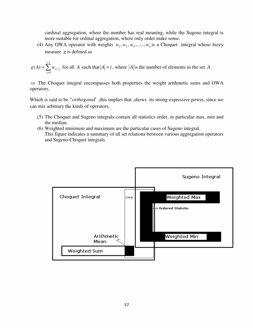
(5) The Choquet and Sugeno integrals contain all statistics order, in particular max, min and
the median.
(6) Weighted minimum and maximum are the particular cases of Sugeno integral.
This figure indicates a summary of all set relations between various aggregation operators
and Sugeno-Choquet integrals.
58
5.9 Application of Choquet Integral
Example 5.1: The teacher of mathematics has to evaluate her students according to their level in
complex analysis, fuzzy logic and numerical analysis. She gives equal importance to complex
analysis and fuzzy logic and less importance to numerical analyses.
The points are given on a scale from 0 to 60.
Students analysisComplex logicFuzzy analysis Numerical
1C 45 50 40
2C 56 35 50
3C 39 58 55
4C 58 38 57
Suppose that the grades of importance is given by
{ } { }{ } { }{ } { } 0.3=)analysis numerical( g=)x(g
0.45=)logicfuzzy ( g =)x(g
0.45=)analysiscomplex ( g = )x( g
3
2
1
λ
λ
λ
By the example 3.8
4492.0−=λ
0.6894 =})x,({x g
0.8090 =})x,({x g
31
21
λ
λ
0.6894 =})x,({x g 32λ
and
{ } 1),,()(g 321 == xxxgX λλ
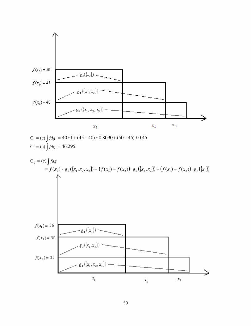
Construction of Choquet Integral
λ∫= fdg(c)C1 )( 3xf= ⋅ { } +),,( 321 xxxgλ ( ) { }( )2131 ,)()( xxgxfxf λ⋅−
( ) { }( )212 )()( xgxfxf λ⋅−+
59
∫= fdg(c)C1= 45.0)4550(8090.0)4045(140 ∗−+∗−+∗
∫= fdg(c)C1295.46=
∫= fdg(c)C 2 )( 2xf= ⋅ { } +),,( 321 xxxgλ ( ) { }( )2323 ,)()( xxgxfxf λ⋅− ( ) { }( )121 )()( xgxfxf λ⋅−+
60
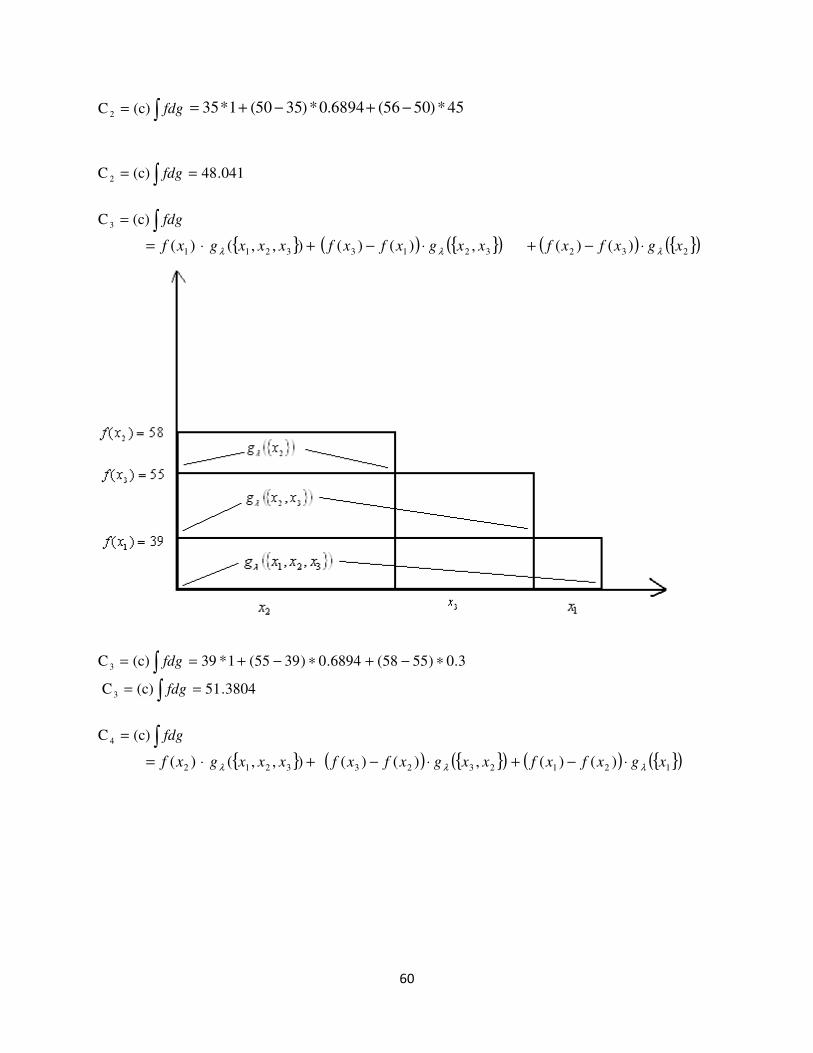
∫= fdg(c)C 245*)5056(6894.0*)3550(1*35 −+−+=
041.48(c)C 2 == ∫ fdg
∫= fdg(c)C 3
)( 1xf= ⋅ { } +),,( 321 xxxgλ ( ) { }( )3213 ,)()( xxgxfxf λ⋅−
( ) { }( )232 )()( xgxfxf λ⋅−+
3.0)5558(6894.0)3955(1*39(c)C 3 ∗−+∗−+== ∫ fdg
3804.51(c)C 3 == ∫ fdg
∫= fdg(c)C 4
)( 2xf= ⋅ { } +),,( 321 xxxgλ ( ) { }( )2323 ,)()( xxgxfxf λ⋅− ( ) { }( )121 )()( xgxfxf λ⋅−+
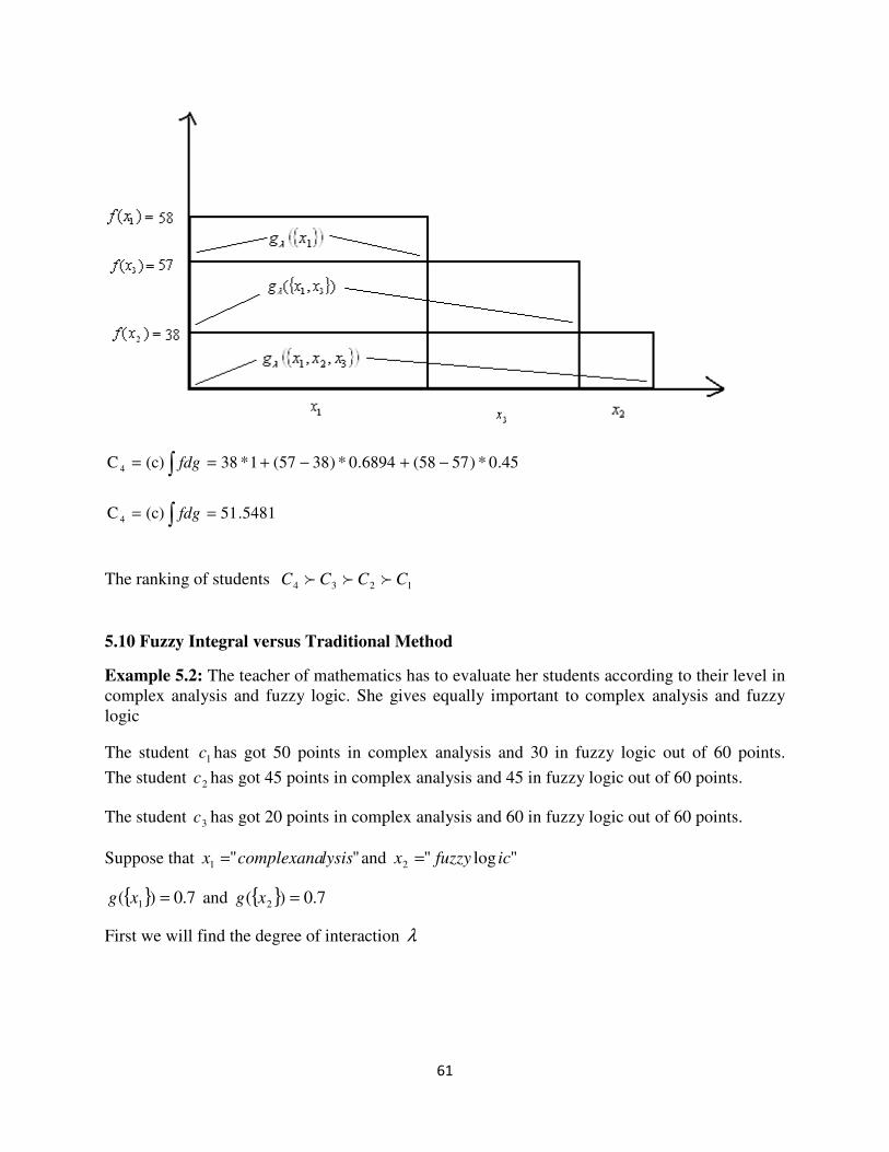
61
45.0*)5758(6894.0*)3857(1*38(c)C 4 −+−+== ∫ fdg
5481.51(c)C 4 == ∫ fdg
The ranking of students 1234 CCCC fff
5.10 Fuzzy Integral versus Traditional Method
Example 5.2: The teacher of mathematics has to evaluate her students according to their level in
complex analysis and fuzzy logic. She gives equally important to complex analysis and fuzzy
logic
The student 1c has got 50 points in complex analysis and 30 in fuzzy logic out of 60 points.
The student 2c has got 45 points in complex analysis and 45 in fuzzy logic out of 60 points.
The student 3c has got 20 points in complex analysis and 60 in fuzzy logic out of 60 points.
Suppose that ""1 lysiscomplexanax = and "log"2 icfuzzyx =
{ } 7.0)( 1 =xg and { } 7.0)( 2 =xg
First we will find the degree of interaction λ
62
According to mathematical reasoning if 1> )(xg2
1i
i∑=
λ then 0, < < 1- λ According to
mathematical reasoning if 1> )(xg2
1i
i∑=
λ then 0, < < 1- λ λ is also called the degree of
interaction.
1+λ = ∏=
n
i 1
)1( igλ+
1+λ = 2)17.0( +λ
λ = 81632.0−
And so 1}),({ 21 =xxgλ
Choquet Integral
447.0*)3050(30*1)(:1 =−+=∫ dgxfC
4545*1)(:2 ==∫ dgxfC
487.0*)2060(20*1)(:3 =−+=∫ dgxfC
The ranking of the above model
3C f 2C f .1C
Now we are introducing weight sum or additive model
1C : 40)7.07.0(
7.0*50
)7.07.0(
7.0*30 =
++
+
2C : 45)7.07.0(
7.0*45
)7.07.0(
7.0*45 =
++
+
3C : 40)7.07.0(
7.0*60
)7.07.0(
7.0*20 =
++
+
2C f 3C = 1C
According to mathematical reasoning if { } { } 1>)()( 11 xgxg + then λ 0< ⇒overestimation in the
grades of importance if we use additive model, then { }
{ } { })()(
)(
21
1
xgxg
xg
+<
{ }{ }),(
)(
21
1
xxg
xg and
63
{ }{ } { })()(
)(
21
2
xgxg
xg
+<
{ }{ }),(
)(
21
2
xxg
xg, and we get an underestimation over evaluation if we use
additive or weight sum model.
Thus if we use λ 0< ,then the criteria relation have the substitutive effect ,impulse we can
enhance the criteria, if we choose the professional skills then the Choquet integral is far more
better than a traditional evaluation method.
5.11 The Application of Choquet and Sugeno Integral in Medical Diagnosis
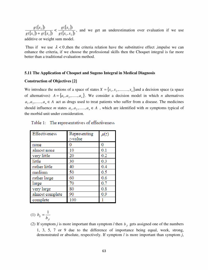
Construction of Objectives [2]
We introduce the notions of a space of states { }nxxxX ,,........., 21= and a decision space (a space
of alternatives) { }naaaA ,......,, 21= . We consider a decision model in which n alternatives
Aaaa n ∈,......,, 21 act as drugs used to treat patients who suffer from a disease. The medicines
should influence m states Aaaa n ∈,......,, 21 , which are identified with m symptoms typical of
the morbid unit under consideration.
(1) jl
ljb
b1
=
(2) If symptom j is more important than symptom l then jlb gets assigned one of the numbers
1, 3, 5, 7 or 9 due to the difference of importance being equal, week, strong,
demonstrated or absolute, respectively. If symptom l is more important than symptom j,
64
we will assign the value of jlb .Having obtained the above judgments an mm× matrix
m
ljjlbB 1,)( == is constructed.
(3) For example 5.4 we will construct the above judgments of )2()2( +×+ mm matrix2
1,)(+== m
ljjlbB
The weights Wwww n ∈,......,, 21 are decided as components of the eigenvector corresponding to
the largest in magnitude eigen value of the matrix B.
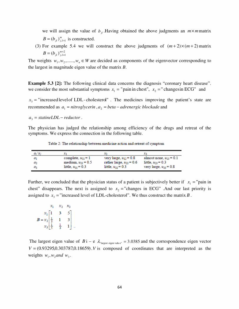
Example 5.3 [2]: The following clinical data concerns the diagnosis “coronary heart disease”.
we consider the most substantial symptoms =1x ,chest"in pain " =2x ” ECG"in changes and
=3x l"cholestero-LDL of level increased" . The medicines improving the patient’s state are
recommended as rinnitroglycea =1 , adrenergicbetaa −=2 blockade and
reductorstatineLDLa −=3 .
The physician has judged the relationship among efficiency of the drugs and retreat of the
symptoms. We express the connection in the following table.
Further, we concluded that the physician status of a patient is subjectively better if =1x ”pain in
chest” disappears. The next is assigned to =2x ”changes in ECG” .And our last priority is
assigned to =3x ”increased level of LDL-cholesterol”. We thus construct the matrix B .
The largest eigen value of B i – e 0385.3"eeigen valulargest " =λ and the correspondence eigen vector
)18659.0,303787.0,93295.0(=V .V is composed of coordinates that are interpreted as the
weights andww 21, 3w .
65
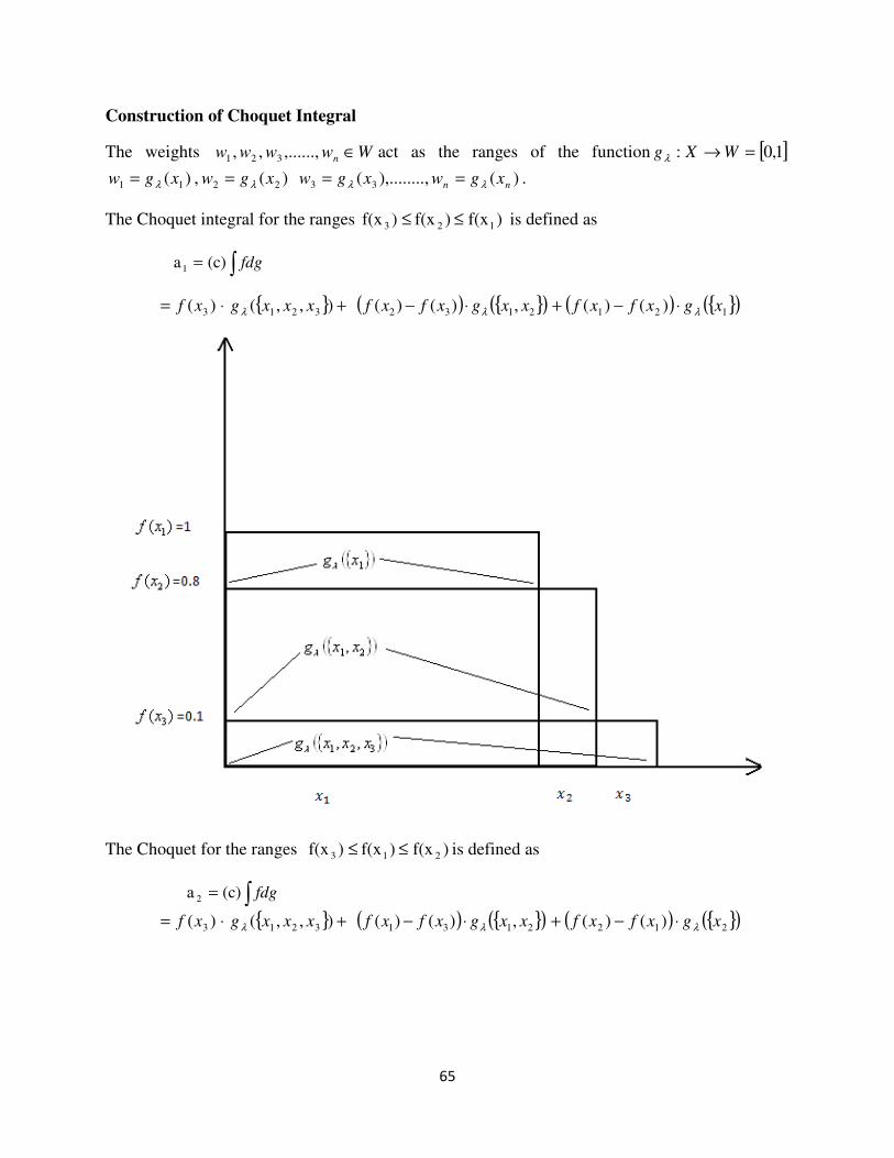
Construction of Choquet Integral
The weights Wwwww n ∈,......,,, 321 act as the ranges of the function [ ]1,0: =→ WXgλ
)( 11 xgw λ= , )( 22 xgw λ= )(,),........( 33 nn xgwxgw λλ == .
The Choquet integral for the ranges )f(x )f(x )f(x 123 ≤≤ is defined as
∫= fdg(c)a1
)( 3xf= ⋅ { } +),,( 321 xxxgλ ( ) { }( )2132 ,)()( xxgxfxf λ⋅− ( ) { }( )121 )()( xgxfxf λ⋅−+
The Choquet for the ranges )f(x )f(x )f(x 213 ≤≤ is defined as
∫= fdg(c)a 2
)( 3xf= ⋅ { } +),,( 321 xxxgλ ( ) { }( )2131 ,)()( xxgxfxf λ⋅− ( ) { }( )212 )()( xgxfxf λ⋅−+
66
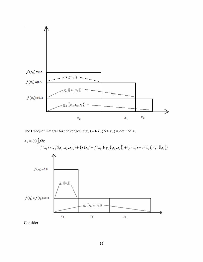
The Choquet integral for the ranges )f(x )f(x )f(x 321 ≤= is defined as
∫= fdg(c)a 3
)( 1xf= ⋅ { } +),,( 321 xxxgλ ( ) { }( )3212 ,)()( xxgxfxf λ⋅− ( ) { }( )323 )()( xgxfxf λ⋅−+
Consider

67
0.18659=})({xg
0.303787=})({xg
0.93295=})({xg
3
2
1
λ
λ
λ
First we calculate the value of λ )n interactio of degree(
Since ( )∏=
+n
1i
i 1g=1+ λλ
1)+1)(0.18659+71)(0.30378+(0.93295=1+ λλλλ
0=0.423290.5141+0.05287 23 λλλ +
And the roots of the above equation will be
0.9082}- {0,-8.81, =λ
But ),1( ∞−∈λ
We will take =λ 0.9082- only, because 0=λ is additively.
If =λ 0.9082- then
= })x,({x 21λg 0.979386=}) ({x})g ({xg}) ({xg +}) ({xg 2121 λλλλ λ+
= })x,({x 32λg 0.438924=}) ({x})g ({xg}) ({xg +}) ({xg 2323 λλλλ λ+
= })x,({x 31λg 0.961496=}) ({x})g ({xg}) ({xg +}) ({xg 3131 λλλλ λ+
1=(X) g λ
∫= fdg(c)a1 )( 3xf= ⋅ { } +),,( 321 xxxgλ ( ) { }( ) ( ) { }( )1212132 )()(,)()( xgxfxfxxgxfxf λλ ⋅−+⋅−
0.97=
0.93295*0.8)-(1+0.9793*0.1)-(.8 +1*0.1 =
∫= fdg(c)a 2 )( 3xf= ⋅ { } +),,( 321 xxxgλ ( ) { }( ) ( ) { }( )2122131 )()(,)()( xgxfxfxxgxfxf λλ ⋅−+⋅−
68
0.52=
0.303*0.5)-(.6+0.96149*0.3)-(0.5 +1*0.3 =
∫= fdg(c)a 3 )( 1xf= ⋅ { } +),,( 321 xxxgλ ( ) { }( ) ( ) { }( )3233212 )()(,)()( xgxfxfxxgxfxf λλ ⋅−+⋅−
0.39=
0.1866*0.3)-(.8+0 +1*0.3 =
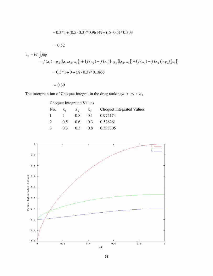
The interpretation of Choquet integral in the drug ranking 321 aaa ff
0.3933050.80.30.33
0.5262610.30.60.52
0.9721740.10.811
Values IntegratedChoquet xxxNo.
Values IntegratedChoquet
321
69
The Sugeno integral in the drug order
Construction of Sugeno integral
{ }( )( ) { }( )( ) { }( )( )( )∫ == 1121232131 ),(min,,),(min,,,),(minmax xgxfxxgxfxxxgxffdga λλλλ
{ }( )( ) { }( )( ) { }( )( )( )∫ == 2221132132 ),(min,,),(min,,,),(minmax xgxfxxgxfxxxgxffdga λλλλ
{ }( )( ) { }( )( ) { }( )( )( )∫ == 3323232113 ),(min,,),(min,,,),(minmax xgxfxxgxfxxxgxffdga λλλλ
( ))93295,.1min(),979386.0,8.0min(),1,1.0min(max1 =a
( )93295.0,8.0,1.0max1 =a
93295.01 =a
( ))93295.0,6.0min(),979386.0,5.0min(),1,3.0min(max2 =a
( )303787.0,5.0,3.0max2 =a
5.02 =a
( ))18659.0,8.0min(),438942.0,3.0min(),1,3.0min(max3 =a
=3a ( )18659.0,3.0,3.0max
3.03 =a
The interpretation Sugeno integral in the drug ranking 321 aaa ff .
Choquet and Sugeno integrals of fuzzy decision process in a choice of optimal medicines.
Construction of Objectives [3]
We introduce the notions of a space of states { }nxxxX ,,........., 21= and a decision space (a space
of alternatives) { }naaaA ,......,, 21= . We consider a decision model in which n alternatives
Aaaa n ∈,......,, 21 act as drugs used to treat patients who suffer from a disease. The medicines
should influence m states Aaaa n ∈,......,, 21 , which are identified with m symptoms typical of
the morbid unit under consideration.
The drugs-decisions constitute n elements in supports of fuzzy sets KK ,
2,+m 1,+m m, ,… 1, =k determined as some criteria-objectives, which restrict the set A [13].
70
Hence, we can treat each set KK
as a fuzzy subset of A, i.e., [ ]1,0: →AK K ,
2.+m 1,+m m, ,… 1, =k [3](More explanation)
In the model of accepting the most optimal medicine ia n, ,… 1, = i we assume that the first m
restriction sets m ,… 1, = j ,K j, are defined by
"=jK onan,......,a of influence 1
n1
1j a
concerningeffect s'......
aconcerningeffect s'
" xsymptom naa++= (1)
In spite of drug effectiveness, which definitely is the most important factor in the appreciation of
drug action, we can introduce other substantial elements assisting drug decision making like side
effects of medicines or their prices. We thus form the next fuzzy set.
=+1mK ofeffect side" naa ,.....,1 "positivelydecision thesupporting =
n
n
1
1
aa ofeffect side-1
........a
a ofeffect side-1++ (2)
in which a physician estimates the strength of all side effects of the drugs. The side effects of
drugs n, ,… 1, = i ,a i are rather unfavorable occurrences; therefore their lack in ia should be
emphasized by the larger membership value as-signed to ai as an indication of a safe medicine
consumption. For the purpose of enlarging membership values of these medicines that have not
extensive side effects we use the complement operation 1–estimation of side effects.
The last constraint
=+2mK ”estimation of price availability for =",.....,1 naa
n
n
1
1
aa ofty availabili price
........a
a ofty availabili price++
(3)
is added in order to enlarge a number of decisive indications.
Not all symptoms retreat after the cure has been carried out. One can only sometimes soothe
their negative effects by, for example, the lowering of an excessive level of the indicator, the
relief of pain, and the like.
Let us find a practical way of determining effectiveness of drugs as mathematical expressions,
which should take place in the first m objectives. To simplify the symbols we assume that each
symptom , where X is a space of symptoms (states), is understood as the result of the treatment of
the symptom after the cure with the drugs na,......,a 1 has been carried out.
Example 5.4 [3]: We have obtained the clinical data, which concerns the diagnosis “coronary
heart disease”. We consider the most substantial symptoms x1
= “pain in chest”, x2
= “changes in
EKG” and x3
= “increased level of LDL-cholesterol”. The recommended medicines that can
71
improve the patient’s state are listed as a1
= nitroglycerin, a2
= beta-adrenergic blockade, a3
=
acetylsalicylic acid (aspirin) and a4
= statine LDL-reductor.
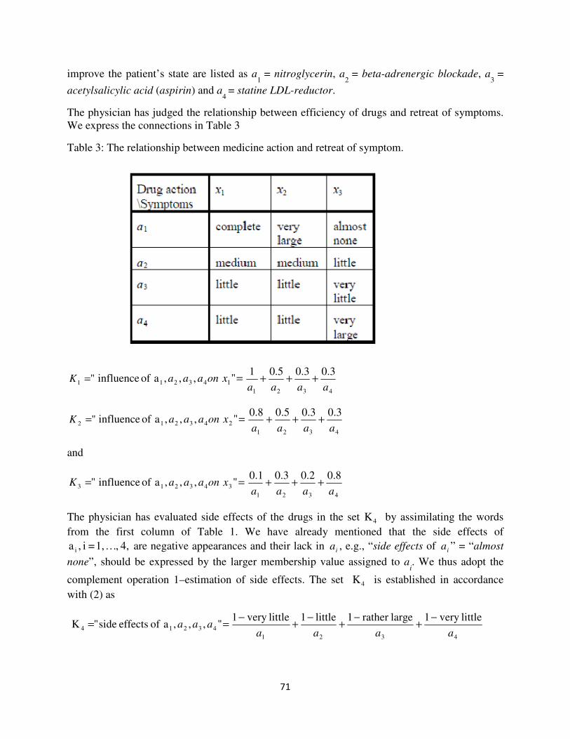
The physician has judged the relationship between efficiency of drugs and retreat of symptoms.
We express the connections in Table 3
Table 3: The relationship between medicine action and retreat of symptom.
"1 =K onaaa 4321 ,,,a of influence ="1x4321
3.03.05.01
aaaa+++
"2 =K onaaa 4321 ,,,a of influence ="2x4321
3.03.05.08.0
aaaa+++
and
"3 =K onaaa 4321 ,,,a of influence ="3x4321
8.02.03.01.0
aaaa+++
The physician has evaluated side effects of the drugs in the set K 4 by assimilating the words
from the first column of Table 1. We have already mentioned that the side effects of
4, ,… 1, = i ,a i are negative appearances and their lack in ia , e.g., “side effects of ia ” = “almost
none”, should be expressed by the larger membership value assigned to ai. We thus adopt the
complement operation 1–estimation of side effects. The set K 4 is established in accordance
with (2) as
4321
43214
littlevery 1largerather 1little 1littlevery 1",,,a of effects side" K
aaaaaaa
−+
−+
−+
−==
72
4321
43214
0.210.610.3 10.21",,,a of effects side" K
aaaaaaa
−+
−+
−+
−==
4321
43214
8.00.47.00.8",,,a of effects side" K
aaaaaaa +++==
The prices of all medicines are not at the least inconvenient for patients to purchase them. If we
note that the large value of a membership degree corresponds to a rather cheap and available
medicine we can state the set K5
by examining (3) as
== ",,,aty availabili price" K 43215 aaa4321
8.00.98.00.8
aaaa+++
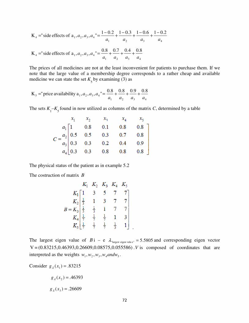
The sets K1–K
5 found in now utilized as columns of the matrix C, determined by a table
The physical status of the patient as in example 5.2
The costruction of matrix B
The largest eigen value of B i – e 5805.5"eeigen valulargest " =λ and corresponding eigen vector
0.055586) 0.08575, 0.26609, 0.46393, (0.83215, = V .V is composed of coordinates that are
interpreted as the weights 54321 ,,, andwwwww .
Consider 83215.)( 1 =xgλ
46393.)( 2 =xgλ
26609.)( 3 =xgλ
73
08575.)( 4 =xgλ
055586.)( 5 =xgλ
Since 1+λ = ∏=
n
i 1
)1( igλ+
so )1055586)(.108575)(.126609.0)(146393.0)(183215.0(1 +++++=+ λλλλλλ
0704166.0957524.02139099.0018085.000494. 2345 =++++ λλλλλ
{ } 0.9046- 3.5974i, - 8.3819- , 3.5974i + 8.3819- 18.9410,- 0,=λ
Since ),1( ∞−∈λ
We will take only 9046.0−=λ
If 9046.0−=λ then
{ } 946897.0),( 21 =xxgλ
{ } 897991.0),( 31 =xxgλ
{ } 618389.),( 32 =xxgλ
{ } 853412.0),( 41 =xxgλ
{ } 51373.0),( 42 =xxgλ
{ } 331224.0),( 43 =xxgλ
{ } 845955.0),( 51 =xxgλ
{ } 496225.0),( 52 =xxgλ
{ } 308319.0),( 53 =xxgλ
{ } 137034.0),( 54 =xxgλ
{ } 985067.0.),,( 321 =xxxgλ
{ } 959198.0),,( 421 =xxxgλ
{ } 914086.0),,( 431 =xxxgλ
74
{ } 656174.0),,( 432 =xxxgλ
{ } 954871.0),,( 521 =xxxgλ
{ } 908424.0),,( 531 =xxxgλ
{ } 642882.0),,( 532 =xxxgλ
{ } 866086.0),,( 541 =xxxgλ
{ } 543487.0),,( 542 =xxxgλ
{ } 370158.0),,( 543 =xxxgλ
{ } 994407.0),,,( 4321 =xxxxgλ
{ } 991122.0),,,( 5321 =xxxxgλ
{ } 966553.0),,,( 5421 =xxxxgλ
{ } 92371.0),,,( 5431 =xxxxgλ
{ } 678767.0),,,( 5432 =xxxxgλ
{ } 1),,,,( 54321 =xxxxxgλ
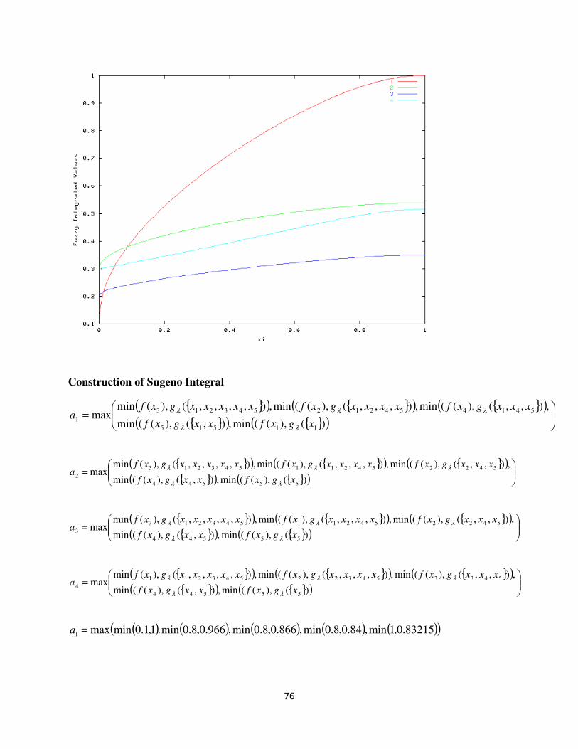
Now construction of Choquet integral
∫= fdg(c)a1
)( 3xf= ⋅ { } +),,,,( 54321 xxxxxgλ ( ) { }( )542134 ,,,)()( xxxxgxfxf λ⋅−
( ) { }( )141 )()( xgxfxf λ⋅−+
∫= fdg(c)a1= 83215.02.0966553.07.011.0 ∗+∗+∗
∫= fdg(c)a1943.0=
∫= fdg(c)a 2)( 3xf= ⋅ { } +),,,,( 54321 xxxxxgλ ( ) { }( )542132 ,,,)()( xxxxgxfxf λ⋅−
( ) { }( ) { })())()((,)()( 5454524 xgxfxfxxgxfxf λλ −+⋅−+
∫= fdg(c)a 2 0.055586*.1+.137034*.2+.966553*.2+.3=
5263.0a 2 =
75
∫= fdg(c)a 3
)( 3xf= ⋅ { } +),,,,( 54321 xxxxxgλ ( ) { }( )542132 ,,,)()( xxxxgxfxf λ⋅−
( ) { }( ) { })())()((,)()( 5454524 xgxfxfxxgxfxf λλ −+⋅−+
∫= fdg(c)a 3 0.055586*.5+.137034*.1+.966553*.1+1.2∗=
3382.0a 3 =
∫= fdg(c)a 4
)( 1xf= ⋅ { } +),,,,( 54321 xxxxxgλ ( ) { }( )54314 ,,)()( xxxgxfxf λ⋅−
∫= fdg(c)a 4 370158.05.013.0 ∗+∗=
0.4851 a 4 =
The interpretation of Choquet integral in the drug ranking 3421 aaaa fff
0.4850770.80.80.80.30.34
0.3381520.90.40.20.30.33
0.5262740.80.70.30.50.52
0.9430290.80.80.10.811
Values IntegratedChoquet x x x x No.
Values IntegratedChoquet
54321x
76
Construction of Sugeno Integral
{ }( ) { }( ) { }( ){ }( ) { }( )
=
)(),((min,),(),((min
,),,(),((min,),,,(),((min,),,,,(),(minmax
11515
541454212543213
1xgxfxxgxf
xxxgxfxxxxgxfxxxxxgxfa
λλ
λλλ
{ }( ) { }( ) { }( ){ }( ) { }( )
=
)(),((min,),(),((min
,),,(),((min,),,,(),((min,),,,,(),(minmax
55544
542254211543213
2xgxfxxgxf
xxxgxfxxxxgxfxxxxxgxfa
λλ
λλλ
{ }( ) { }( ) { }( ){ }( ) { }( )
=
)(),((min,),(),((min
,),,(),((min,),,,(),((min,),,,,(),(minmax
55544
542254211543213
3xgxfxxgxf
xxxgxfxxxxgxfxxxxxgxfa
λλ
λλλ
{ }( ) { }( ) { }( ){ }( ) { }( )
=
)(),((min,),(),((min
,),,(),((min,),,,(),((min,),,,,(),(minmax
55544
543354322543211
4xgxfxxgxf
xxxgxfxxxxgxfxxxxxgxfa
λλ
λλλ
( ) ( ) ( ) ( ) ( )( )83215.0,1min,84.0,8.0min,866.0,8.0min,966.0,8.0min.1,1.0minmax1 =a
77
)83215.0,8.0,8.0,8.0,1.0max(1 =a
83215.01 =a
( ) ( ) ( )( ) ( )05586.0,8.0min,137034.0,7.0min(,453.0,5.0min,966.0,5.0min,1,3.0minmax2 =a
)05586.0,1347034.0,453.0,5.0,3.0max(2 =a
5.02 =a
( ) ( ) ( )( ) ( )05586.0,9.0min,137034.0,4.0min(,453.0,3.0min,966.0,3.0min,1,2.0minmax3 =a
)05586.0,137034.0,3.0,3.0,2.0max(3 =a
3.03 =a
( ) ( ) ( )( ) ( )05586.0,8.0min,137034.0,8.0min(,370158.0,8.0min,678.0,3.0min,1,3.0minmax4 =a
)05586.0,137034.0,370158.0,3.0,3.0max(4 =a
370158.04 =a
The interpretation of Sugeno integral in the drug ranking 3421 aaaa fff
78
Conclusion
In typical multi-attribute evaluation process, each attribute must be independent from each other.
Therefore the characteristics that have interaction among the criteria in real system cannot be
solved by the concept of tradition additives measure alone. This review has shown the richness
of these new tools for aggregation, the Sugeno-Choquet integrals. Consequently the hierarchical
structure evaluation system of human subjective decision making by using fuzzy−λ measures
and Choquet-Sugeno integrals. I hope that this will encourage mathematician to use this
technique in multi-criteria decision making.
79
RERENCES
[1] Elisabeth Rakus-Andersson: Fuzzy and Rough Techniques in Medical Diagnosis and
Medication, Springer-Verlag, Berlin Heidelberg, 2007.
[2] Elisabeth Rakus-Andersson, Claes Jogreus: The Choquet and Sugeno Integrals as Measures
of Total Effectiveness of Medicines. In: Theoretical Advances and Applications of Fuzzy
Logic and Soft Computing (Proceedings of IFSA 2007, Cancun, Mexico), eds: Oscar
Castillo, Patricia Melin, Oscar Montiel Ross, Roberto Sepulveda Cruz, Witold Pedrycz,
Janusz Kacprzyk, Springer-Verlag, Advances in Soft Computing 42, 2007, pp. 253-262.
[3] Rakus-Andersson Elisabeth : Minimization of Regret versus Unequal Multi-objective Fuzzy
Decision Process in a Choice of Optimal Medicines. Proceedings of the XIth
International
Conference IPMU 2006 – Information Processing and Management of Uncertainty in
Knowledge-based Systems, vol. 2, Edition EDK, Paris-France, 2006, pp 1181-1189
[4] Yu-Ping Ou Yanga, Chin-Tsai Lin
b, Chie-Bein Chen
c, Gwo-Hshiung Tzeng
*
aCivil Aeronautics Administration Ministry of Transportation and Communications, No.340
Tung Hwa N.RD. Taipei, Taiwan bYuanpei University of Science and Technology, No. 306, Yuanpei St., Hsinchu 300,
Taiwan cInstitute of International Business, National Dong Hwa University, 1, Sec. 2,Da Hsueh Rd.,
Shou-Feng, Hualien,Taiwan *Institute of Management of Technology and Institute of Traffic and Transportation,
National Chiao Tung University, 1001 Ta-Hsueh Road, Hsinchu 300, Taiwan
[5] Luis Garmendia Facultad de Informática, Dep. Sistemas Informáticos y
Programación,Universidad Complutense of. Madrid, Spain, E-mail:[email protected],
Web Page: www.fdi.ucm.es/profesor/lgarmend
[6] M.Sugeno and K.Ishii Department of systems science, Tokyo Institute of ,4259 Nagatsuta,
Midori-ku, Yokyohama,227 Japan 1983
[7] Murofushi, T. and Sugeno, M. (1991), “A theory of fuzzy measures. Representation, the
Choquet integral and null sets,” Journal of Mathematical Analysis and Applications, Vol.
159, pp. 532-549.
[8] Michel Grabisch Thomson-CSE Central Research Laboratory, Domaine de Corbeville,
91404 Orsay cedex, France1995
[9] Eiichiro Takahagi Visiting Fellow, University of Bristol, UK (Until August 2005) School of
Commerce, Senshu University, Japan Email: [email protected] March 8, 2005
80
[10] L.A.ZADEH department of Electrical Engineering and Electronics Research Laboratory,
University of California, Berkeley, California 1965
[11] Bartle, Robert G. (1995). The elements of integration and Lebesgue measure. Wiley
Classics Library. New York: John Wiley & Sons Inc.. xii+179
[12] Bourbaki, Nicolas (2004). Integration. I. Chapters 1–6. Translated from the 1959, 1965
and 1967 French originals by Sterling K. Berberian. Elements of Mathematics (Berlin).
Berlin: Springer-Verlag. xvi+472. ISBN 3-540-41129-1. MR2018901
[13] Bourbaki, Nicolas (2004). Integration. I. Chapters 1–6. Translated from the 1959, 1965
and 1967 French originals by Sterling K. Berberian. Elements of Mathematics (Berlin).
Berlin: Springer-Verlag. xvi+472. ISBN 3-540-41129-1. MR2018901
[14] Lee, K. M. and Leekwang, H. (1995), “Identification of λ -fuzzy measure by genetic
algorithms,” Fuzzy Sets and Systems, Vol. 75, No. 3, pp. 301-309.
[15] Interactive Real Analysis, ver. 1.9.5(c) 1994-2007, Bert G. Wachsmuth Mar 26, 2007


![[halshs-00267932, v1] A decade of application of the ... · Sugeno integrals in multi-criteria decision aid ... and practical tools we have now at our dispos al for ... complexity](https://img.pdfslide.net/doc/110x75/5bdc2cbe09d3f248078d53c5/halshs-00267932-v1-a-decade-of-application-of-the-sugeno-integrals-in.jpg)