A Numerical Tool for Flow Simulationin a Wankel Motor

Rolf Rannacher and Vincent Heuveline

Institut rur Angewandte Mathematik, Universitiit Heidelberg,INF 294, 69120 Heidelberg, GermanyE-mail: vincent.heuveline(Qiwr.uni-heidelberg.deE-mail: rolf.rannacher(Qiwr.uni-heidelberg.de

Abstract. We describe the main steps in the development of a new numericaltool for simulating gas flow and heat transfer in a rotary engine ("Wankel motor").Our approach comprises a 2D/3D grid generator for the Wankel motor geometry,an implicit finite element discretization for coping with the stiff pressure-velocitycoupling and robust multigrid solvers on strongly distorded meshes. These compo­nents are implemented within a new FE-software package named Hi-Flow++ whichis presently under development.

1 Description of the Project

The aim of this project is to construct a numerical tool for the simulationof gas flow and heat transfer in a rotary engine ("Wankel motor", Fig. 1).Particular numerical difficulties are caused by the extreme geometry changesand the inherent stiffness due to "low-Mach-number" flow conditions. Thelatter requires the use of an implicit solution approach which is orientated bythe incompressible limit case. Many commercial codes are inefficient undersuch conditions since they are mostly based on explicit methods which maybe appropriate at higher Mach number but fail for Ma -+ 0 and on highlyanisotropic meshes.The first results of this project are the implementation of a 2D/3D grid

generator for the Wankel motor geometry and the various components for aNavier-Stokes solver adapted to this special configuration. This particularlycomprises a finite element discretization of higher order, an implicit pressure­velocity coupling as well as the treatment of strongly varying anisotropicmeshes. To this end, a new finite element software package, Hi-Flow++, hasbeen developed which is particularly designed for flow problems on locallyrefined and possibly distorded meshes in 2D as well as 3D geometries. Atthe moment, the 2D version of the code has been completed which solvesbesides various model equations in particular the stationary compressibleNavier-Stokes equations in the low-Mach-number approximation. The cur­rent steps in this project are the extension to nonstationary flows and theimplementation of the basic ingredients for the 3D solver. For the latter themain components like mesh handling, assembling of system matrices, meshtransfer operations and mesh-point renumbering have already been realized.

W. Jäger et al. (eds.), Mathematics - Key Technology for the Future© Springer-Verlag Berlin Heidelberg 2003

34 R. Rannacher and V. Heuveline

1.1 The Wankel Motor

Unlike the conventional combustion engines with reciprocating piston motion,the Wankel Rotary Combustion Engine (RCE) is based on the continuousrotation of the so-called rotor [BEN,AB]. It has four phases in its combustioncycle: intake, compression, power and exhaust.

Fig. 1. Four combustion phases: intake, compression, power and exhaust

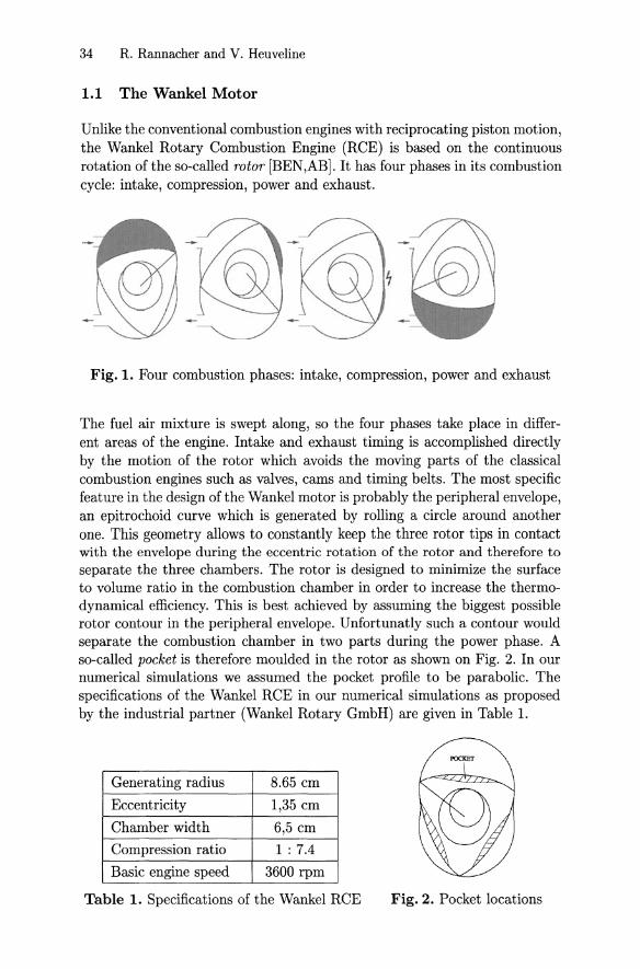
The fuel air mixture is swept along, so the four phases take place in differ­ent areas of the engine. Intake and exhaust timing is accomplished directlyby the motion of the rotor which avoids the moving parts of the classicalcombustion engines such as valves, cams and timing belts. The most specificfeature in the design of the Wankel motor is probably the peripheral envelope,an epitrochoid curve which is generated by rolling a circle around anotherone. This geometry allows to constantly keep the three rotor tips in contactwith the envelope during the eccentric rotation of the rotor and therefore toseparate the three chambers. The rotor is designed to minimize the surfaceto volume ratio in the combustion chamber in order to increase the thermo­dynamical efficiency. This is best achieved by assuming the biggest possiblerotor contour in the peripheral envelope. Unfortunatly such a contour wouldseparate the combustion chamber in two parts during the power phase. Aso-called pocket is therefore moulded in the rotor as shown on Fig. 2. In ournumerical simulations we assumed the pocket profile to be parabolic. Thespecifications of the Wankel RCE in our numerical simulations as proposedby the industrial partner (Wankel Rotary GmbH) are given in Table 1.

Generating radius 8.65 cm

Eccentricity 1,35 cm

Chamber width 6,5 cm

Compression ratio 1:7.4

Basic engine speed 3600 rpm

Table 1. Specifications of the Wankel RCE Fig. 2. Pocket locations

Flow Simulation in the Wankel Motor 35

The maximum rotation velocity of this prototype is approximatly Vmax ~

30 m/s which corresponds to a flow behavior in the low-Mach-number rangeas Mamax < 0.1 in this case. Accordingly acoustic waves may be neglectedwhich is achieved by the "low-Mach-number" approximation of the compress­ible Navier-Stokes equations.

1.2 The Mathematical Model

The flow in the rotary engine is described by the compressible Navier-Stokesequations in the "low-Mach-number" approximation. Here, the pressure pis split into a thermodynamic part Pth which is constant in space and ahydrodynamic part Phyd, while only the latter one is used in the equationof state (see e.g. [MAJ]). Due to the temporal variation of the domain, thethermodynamic pressure is time dependent, too. We denote by Dt := Ot+v,V'the material derivative. The whole system of equations written in primitivevariables takes the following form:

T- 1DtT - V'·v

pDtV - V'. (J.UT) + V'Phyd

pCpDtT - V' {XV'T) - OtPhyd - J..l!7: V'v

= pthlatpth

Pfe

= OtPth

(1)(2)

(3)

where !7 := (V'v+ V'vT) - ~(V' ·v)l, cp, >., fe, and J..l represent the shear­

stress tensor, the heat capacity, the heat conductivity, the volume forces andthe dynamic shear viscosity, respectively. The equation of state is given by

(4)

The time derivative of Pth is obtained by first averaging the continuityequation (1) in space and then substituting D tT by using (4), whereas theheating due to Phyd and J..l!7: V'v is neglected. This leads to the followingscalar ODE for Pth :

where Pth(O) = Po is a given initial value. Our numerical approach to sys­tem (1)-(3) is based on its "variational" formulation which will be brieflydescribed below. Let, (.,.) denote the usual L2-scalar product on [l. fur­ther, Hl([l) is the space of L2-functions with generalized (in the sense ofdistributions) first-order derivatives in L2([l). This is the only notation frommathematical theory of function spaces we are going to use in this paper.The variational formulation of the stationary form of the system (1)­

(3) is obtained by multiplying the equations by appropriate test functions{X, ,¢, 7f} =: ¢ and integrating over the domain [l. This leads us to define

36 R. Rannacher and V. Heuveline

the stationary semi-linear form a(·;·) by

a(u;¢) := (T-1v·VT,X) - (V·v,X)

+ (p(v·V)v,'lj;) + (j.LVV, V'lj;) - (Phyd - ~j.LV·v, V·'lj;) - (P!e,'lj;)+ (pcpv·VT,1r) + ()..VT, V1r) - (j.L(j:VV,1r).

In the diffusive terms, we have used integration by parts. Neumann-typeboundary conditions are implicitly represented by the variational formulation,while Dirichlet boundary conditions have to be explicitly imposed on thesolution. The variational form of system (1)-(3) then reads in short terms:Find u(t) := {T(t), V(t),Phyd(t)} E V +Ub, such that u(O) = Uo and

(QOtU, ¢) + a(u; ¢) = F(¢) V¢ E V. (6)

where Q is a suitable coefficient matrix multiplying the time derivatives. Theright-hand side F(·) contains the slave variable Pth given by the relation(5), while P is determined through the modified gas law (4). The termUb represents prescribed boundary data. The function space V in whichU - Ub is sought is the tensor product of certain subspaces of H 1([]) fortemperature and velocity while the space for the hydrodynamic pressure isL2 ([]) . If Dirichlet conditions for the velocity are imposed along the entireboundary, the hydro-dynamic pressure is only defined modulo a constant andthe corresponding pressure-space is L2 ( []) / R.

2 The Solution Approach

2.1 The Galerkin Finite Element Discretization

Our Navier-Stokes solver uses a fully implicit approach for solving the "low­Mach-number" approximation of the compressible Navier-Stokes system (6)(for a detailed description we refer to [BBR], [BR]).The Galerkin finite element method is defined on quadrilateral/hexahedral

meshes 7 h = {K} covering the domain t'l. The trial and test spaces Vh C Vconsist of continuous, piecewise polynomial vector functions (so-called Qp­elements) for all unknowns,

Vh = {{T,v,p} E C(t'l)1+dH IT,vIK E Q~+d,pIK E Qs},

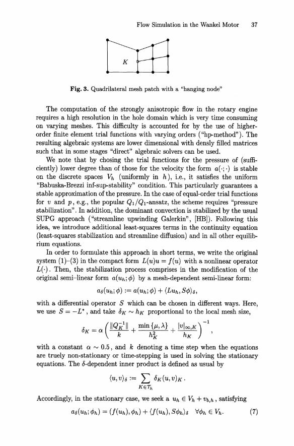
where s = 1 for r = 2, and s = r - 2 for r ~ 3. Here, Qr is the spaceof (isoparametric) tensor-product polynomials of degree r (for a detailed de­scription of this standard construction process see [BS]). In order to facilitatelocal mesh refinement and coarsening, we allow the cells in the refinementzone to have nodes which lie on faces of neighboring cells (Fig. 3). The degreesof freedom corresponding to such "hanging nodes" are eliminated from thesystem by interpolation inforcing global conformity (Le., continuity acrossinterelement boundaries) for the finite element functions. For simplicity, wedo not allow varying polynomial order accross hanging nodes.

Flow Simulation in the Wankel Motor 37

K

Fig. 3. Quadrilateral mesh patch with a "hanging node"

The computation of the strongly anisotropic flow in the rotary enginerequires a high resolution in the hole domain which is very time consumingon varying meshes. This difficulty is accounted for by the use of higher­order finite element trial functions with varying orders ("hp-method"). Theresulting algebraic systems are lower dimensional with densly filled matricessuch that in some stages "direct" algebraic solvers can be used.We note that by chosing the trial functions for the pressure of (suffi­

ciently) lower degree than of those for the velocity the form a(·;·) is stableon the discrete spaces Vh (uniformly in h), i.e., it satisfies the uniform"Babuska-Brezzi inf-sup-stability" condition. This particularly guarantees astable approximation of the pressure. In the case of equal-order trial functionsfor v and p, e.g., the popular Ql/Q1-ansatz, the scheme requires "pressurestabilization" . In addition, the dominant convection is stabilized by the usualSUPG approach ("streamline upwinding Galerkin", [HB]). Following thisidea, we introduce additional least-squares terms in the continuity equation(least-squares stabilization and streamline diffusion) and in all other equilib­rium equations.In order to formulate this approach in short terms, we write the original

system (1)-(3) in the compact form L(u)u = f(u) with a nonlinear operatorL(·). Then, the stabilization process comprises in the modification of theoriginal semi-linear form a(uh; </J) by a mesh-dependent semi-linear form:

a6(uh; </J) := a(uh; </J) + (LUh, S</J)6,

with a differential operator S which can be chosen in different ways. Here,we use S = -L*, and take 8K '" hK proportional to the local mesh size,

1: _ (11QK111 min{JL,A} IVloo,K)-l

UK - a k + h'k + hK

'

with a constant a '" 0.5, and k denoting a time step when the equationsare truely non-stationary or time-stepping is used in solving the stationaryequations. The 8-dependent inner product is defined as usual by

(U,V)6:= L 8K(u,V)K.KE/h

Accordingly, in the stationary case, we seek a Uh E Vh + Vb,h , satisfying

38 R. Rannacher and V. Heuveline

Clearly, this ansatz is "consistent" in the sense that the additional termsvanish at the exact solution. This modification serves several purposes: itstabilizes the pressure in the low-Mach-number approximation, it stabilizesthe possibly strong convection in the flow, and finally it enhances local massconservation. This leads to a stable scheme for a wide range of flow conditions.

2.2 Solution of the Algebraic Systems

The nonlinear algebraic system (7) is solved by the damped Newton method.Denoting the derivative of a(·;·) taken at a discrete function Uh E Vh bya'(uh;', '), the arising linear systems have the form

Here, w~ is the correction and r~ the equation residual of the precedingapproximation u~. The updates u~+l := u~ + w~ are carried until con­vergence. The linear subproblems (8) are solved by the GMRES methodwith preconditioning by a multigrid iteration. This multigrid component usesblockwise Gauss-Seidel or ILU smoothing in which the physical unknownsare implicitly coupled on the cell level. For a description of the details of thisapproach, we refer to [BR]. In computing really nonstationary flows this tidecoupling may be lifted by "operator splitting" due to the better conditioningin this case.

2.3 Tests of Solver Components

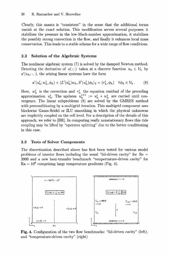
The discretization described above has first been tested for various modelproblems of interior flows including the usual "lid-driven cavity" for Re =2000 and a new heat-transfer benchmark "tempertature-driven cavity" forRa = 106 comprising large temperature gradients (Fig. 4).

v= l6x'(1 -x)' adiabatic / v =0

V(O,y) = 0 v(l,y) =0

TIwt = 960K

v=oT""d ~ 240K

v=o

0.5U====ad:zi.=b.='i=C/=V<::==O===:::zI

x

Fig. 4. Configuration of the two flow benchmarks: "lid-driven cavity" (left),and "temperature-driven cavity" (right)

Flow Simulation in the Wankel Motor 39

Discretization by higher-order finite elements. Table 2 shows somerepresentative results for the simple test case "lid-driven cavity" , while thosefor the harder test case "heat-driven cavity" are presented in Table 3. Itturns out that higher-order finite elements have good potential for accuratelycomputing interior flows even in the presence of strong layers. The solution ofthe algebraic problems is the bottleneck in using higher-order finite elementswithin implicit flow solvers. This problem is tackled by using hierarchicalmultilevel techniques with blockwise smoothers. However, further develop­ment is necessary at this point to reach fully satisfactory solution efficiency.

I FE ansatz I Fr(Uh) I #cells I #dofs I #entries I CPU IQ2/Q1 -0.08657 16,384 14,8739 5,994,249 2,100 sQ3/Q1 -0.08657 4,096 78,723 4,537,737 1,620 sQ4/Q2 -0.08657 1,024 37,507 3,237,897 3,240 sQ6/Q4 -0.08657 256 23,043 3,701,769 4,620 sQ8/Q6 -0.08658 64 10,851 2,779,785 5,400 s

Table 2. Efficiency of higher-order finite elements for solving the "lid-driven cavity"problem with Re = 2000 (error rv 1%)

CPU IQ2/Q1 8.843 16,384 214,788 12,069,136 12,324 sQ3/Q1 8.859 4,096 115,972 9,558,544 8,765 sQ4/Q2 8.871 1,024 54,148 6,587,904 7,484 sQ5/Q3 8.893 256 22,084 3,707,536 6,843 s

I FE ansatz I N(Uh) I #cells I #dofs I # entries I

Table 3. Accuracy of higher-order finite elements for solving the "temperature­driven cavity" problem with Ra = 106 (error rv 1%)

~,I

\

:.~~

......·.­........·~·...............·....

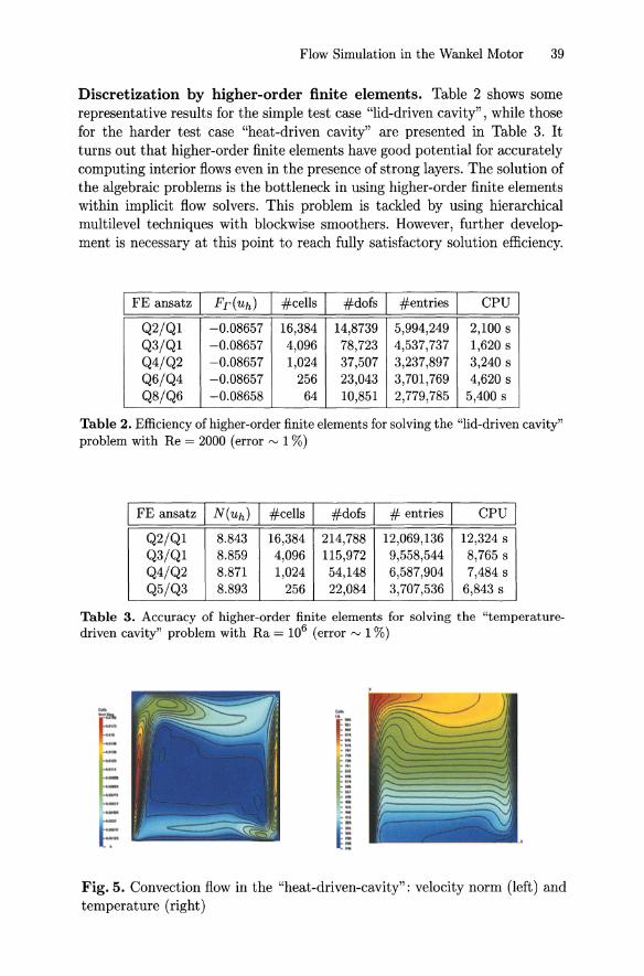
Fig. 5. Convection flow in the "heat-driven-cavity": velocity norm (left) andtemperature (right)

40 R. Rannacher and V. Heuveline

The time stepping. The simulation of the fully nonstationary flow behaviorin the rotary engine, at first, requires a geometric description of the chambermovement. This is obtained in terms of a transformation <P~' between thetime-dependent domains,

Instead of working on a fixed domain, we consider a variational formulationand discretization on the deforming domain, nt, i.e. the L2-scalar productsin (6) are considered on !tt (see [LTD. The discretization is applied in twosteps: A spatial semi-discretization of (6) leads to a set of ordinary differentialequations which is solved by using a stiffiy-stable time stepping scheme like,for example the implicit Euler, the damped Crank-Nicholson, or the second­order Fractional-Step-O scheme. Compared to the usual formulation on afixed domain here an additional term has to be added in the variationalformulation (6) which represents the time-variation of the domain nt . Afterspatial semi-discretization this results in the ODE system

for all <Ph E Vh, with the so-called "mesh-velocity operator" N(t). Thisoperator corresponds to the matrix

where IJtt := <I>;l , with Jacobian DlJtt , and {4>di=l,. .. ,1 is a basis of the finiteelement space on the mesh for nt ,. In order to cope with (time dependent)local singularities arising at the intake and exhaust, we use local mesh refine­ment in these areas (Fig. 7). The mesh refinement is driven by local "errorindicators" derived heuristically from properties of the computed solution.

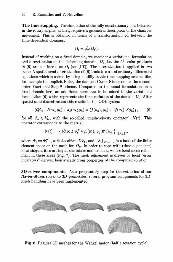
3D-solver components. As a preparatory step for the extension of ourNavier-Stokes solver to 3D geometries, several program components for 3D­mesh handling have been implemented:

Fig. 6. Regular 3D meshes for the Wankel motor (half a rotation cycle)

Flow Simulation in the Wankel Motor 41

- a mesh generator for the Wankel motor configuration (see Fig. 6),- administration of locally refined meshes,- assembling of system matrices,- mesh transfer operations for multigrid and mesh numbering.

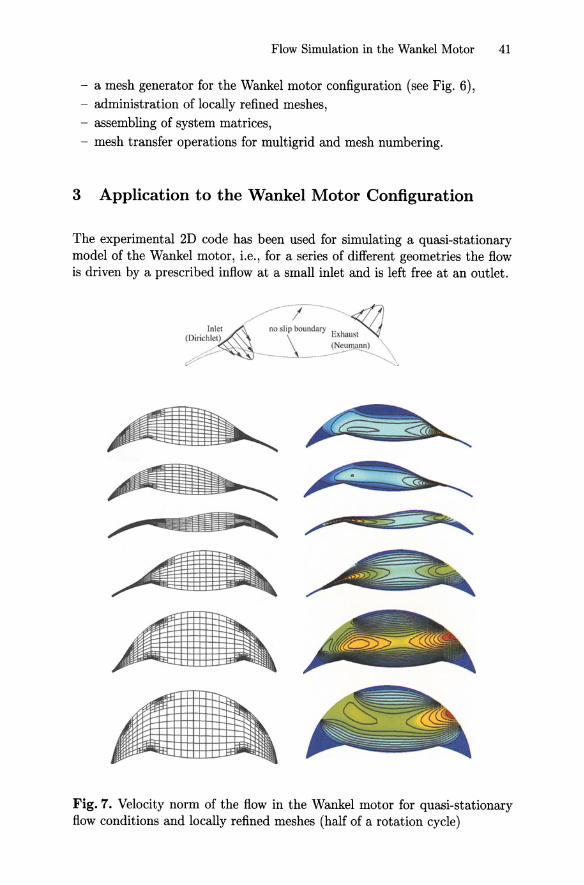
3 Application to the Wankel Motor Configuration

The experimental 2D code has been used for simulating a quasi-stationarymodel of the Wankel motor, Le., for a series of different geometries the flowis driven by a prescribed inflow at a small inlet and is left free at an outlet.

Inlet(Dirichlet)

/ ..... Ino lip boundary E~hausl

( eu ann)--

Fig. 7. Velocity norm of the flow in the Wankel motor for quasi-stationaryflow conditions and locally refined meshes (half of a rotation cycle)

42 R. Rannacher and V. Heuveline

4 Conclusion and Outlook

We have described the main components of a new numerical tool for simu­lating gas flow and heat transfer in a rotary engine. The method is basedon the low-Mach-number approximation of the compressible Navier-Stokesequations and uses a least-squares stabilized finite element discretization ofvariable order. For the sake of robustness the approach is fully implicit andlargly exploits multi-level techniques. At first, a "stationary" flow solver hasbeen developed for interior flows in simple geometries. The natural convectionin a box under strong temperature gradients is a prototypical test case. Then,similar computations have been performed for the (still stationary) "Wankelmotor" in 2D. The next step is the integration of this quasi-stationary solvercomponent into a time-stepping scheme for computing really nonstationaryflows following the variation of the domain. Subsequently, a first 3D versionof the code will be compiled.

References

[AB] J. Abraham, D. Ramoth, J. Mannisto, 3-D steady-state wall heat flux andthermal analysis of a stratified-charge rotary engine, SAE, Society of AutomativeEngineers, Technical Paper Series, Nr. 910706, 1991.

[BEN] W.-D. Bensinger, Rotationskolben- Verbrennungsmotoren, Springer-Verlag,1973.

[BBR] R. Becker, M. Braack, R. Rannacher: Numerical simulation of laminarflames at low Mach number by adaptive finite elements, Combust. Theory Mod­elling. 3, 503-534, 1999.

[BR] M. Braack, R. Rannacher, Adaptive finite element methods for low-Mach­number flows with chemical reactions, Lecture Series 1999-03, 30th Computa­tional Fluid Dynamics, The von Karman Institute, Belgium, 1999.

[BS] S. C. Brenner and R. L. Scott (1994), The Mathematical Theory of FiniteElement Methods, Springer, Berlin-Heidelberg-New York.

[HB] T. J. R. Hughes and A. N. Brooks, Streamline upwind/Petrov-Galerkin for­mulations for convection dominated flows with particular emphasis on the in­compressible Navier-Stokes equation, Comput. Meth. Appl. Mech. Engrg., 32,pp. 199-259, 1982.

[HRS] P. Houston, R. Rannacher, E. Siili: A posteriori error analysis for stabilisedfinite element approximations of transport problems, Preprint 99-26, SFB 359,University of Heidelberg, to appear in J. Comput. Mech. (1999).

[LT] P. Lesaint and R. Touzani: Approximation of the heat equation in a variabledomain with application to the Stefan problem, SIAM J. Numer. Anal. 26, 366­379 (1989).

[MAJ] A. Majda, Compressible fluid flow and systems of conservation laws in sev­eral space varables Springer-Verlag, New York, 1984.

[Rl] R. Rannacher: Adaptive finite element methods for flow problems, Proc. 88thInt. Symp. on Comput. Fluid Dynamics, Bremen, Sept. 5-10, 1999, to appear inJ. Japan Society of CFD.

[R2] R. Becker, M. Braack, R. Rannacher: Adaptive finite element methods forflow problems, Proc. Foundations of Computational Mathematics 99, CambridgeUniversity Press 2000