Graz University of Technology

Christina Gsaxner, BSc

Automatic urinary bladdersegmentation in CT images using

deep learning

MASTER’S THESISto achieve the university degree of

Diplom-IngenieurinMaster’s degree programme: Biomedical Engineering

submitted to

Graz University of Technology

Supervisor

Univ.-Prof. Dipl.-Ing. Dr.techn. Dieter Schmalstieg

Institute of Computer Graphics and Vision8010 Graz, Inffeldgasse 16/II

Advisor

Dr.rer.physiol. Dr.rer.nat. Jan Egger

Graz, October 2017

Affidavit

I declare that I have authored this thesis independently, that I have notused other than the declared sources/resources, and that I have explicitlyindicated all material which has been quoted either literally or by contentfrom the sources used. The text document uploaded to TUGRAZonline isidentical to the present masters thesis.

Date Signature

Eidesstattliche Erklarung

Ich erklare an Eides statt, dass ich die vorliegende Arbeit selbststandig ver-fasst, andere als die angegebenen Quellen/Hilfsmittel nicht benutzt, unddie den benutzten Quellen wortlich und inhaltlich entnommenen Stellen alssolche kenntlich gemacht habe. Das in TUGRAZonline hochgeladene Textdoku-ment ist mit der vorliegenden Masterarbeit identisch.

Datum Unterschrift

i

Abstract

We present an approach for fully automatic urinary bladder segmentation inCT images with artificial neural networks in this thesis. Automatic medi-cal image analysis has become an invaluable tool in the different treatmentstages of diseases. Especially medical image segmentation plays a vital role,since segmentation is often the initial step in an image analysis pipeline.Since deep neural networks have made a large impact on the field of imageprocessing in the past years we use two different deep learning architec-tures to segment the urinary bladder. Both of these architectures are basedon pre-trained classification networks that are adapted to perform semanticsegmentation. Since deep neural networks require a large amount of trainingdata, specifically images and corresponding ground truth labels, we further-more propose a method to generate such a suitable training data set fromPositron Emission Tomography/Computed Tomography image data. This isdone by applying thresholding to the Positron Emission Tomography data forobtaining a ground truth and by utilizing data augmentation to enlarge thedataset. In this thesis, we discuss the influence of data augmentation on thesegmentation results, and compare and evaluate the proposed architecturesin terms of qualitative and quantitative segmentation performance. The re-sults presented in this thesis allow concluding that deep neural networks canbe considered a promising approach to segment the urinary bladder in CTimages.

Keywords: Image Segmentation, Deep Learning, Convolutional Neural Net-works, Urinary Bladder, Computed Tomography

ii

Kurzfassung

In dieser Arbeit wird eine Methode zur vollautomatischen Harnblasenseg-mentierung in Computertomographiebildern mit kunstlichen neuronalen Net-zen vorgestellt. Die automatisierte Analyse von medizinischen Bilddatenhat sich als wertvolles Instrument in verschiedensten Behandlungsstadienvon Krankheiten etabliert. Vor allem die Segmentierung von medizinischenBildern spielt dabei eine wichtige Rolle, da sie oft den ersten Schritt in einerBildanalysepipeline darstellt. Da tiefe, neuronale Netze in den letzten Jahrensehr erfolgreich im Bereich der Bildverarbeitung angewandt wurden, wer-den auch in dieser Arbeit ”Deep Learning” Algorithmen zur Harnblasenseg-mentierung verwendet. Genauer werden zwei unterschiedliche Architekturensolcher Netze vorgestellt, die auf vortrainierten Klassifizierungsnetzwerkenberuhen, welche fur semantische Bildsegmentierung adaptiert werden. Dasolche Netze eine große Anzahl an Daten benotigen, um von ihnen zu ler-nen, wird in dieser Arbeit ebenfalls ein Ansatz zur Generierung eines solchenDatensatzes aus Positronenemmissionstomopgraphie/Computertomographie-Bilddaten vorgestellt. Dabei wird durch ein Schwellenwertverfahren, welchesauf die Positronenemmissionstomographie Bilder angewandt wird, eine Ref-erenzsegmentierung gewonnen. Zusatzlich soll durch Augmentation der Bilderder Datensatz vergroßert werden. Der Einfluss von augmentierten Datenauf das Ergebnis der Segmentierung wird in der Arbeit diskutiert. Auer-dem werden die vorgestellten Netzwerkarchitekturen bezuglich ihrer quali-tativen und quantitativen Segmentierungsergebnissen ausgewertet und ver-glichen. Die Arbeit kommt zu dem Schluss, dass tiefe neuronale Netze einenvielversprechenden Ansatz zur Segmentierung der Harnblase in CT Bilderndarstellen.

Schlusselworter: Bildsegmentierung, Deep Learning, Convolutional NeuralNetwork, Harnblase, Computertomographie

iii

Acknowledgements

I would like to start by thanking my supervisor from the Graz University ofTechnology, Univ.-Prof. Dipl.-Ing. Dr.techn. Dieter Schmalstieg, for givingme the opportunity to carry out this work in his department and for providingthe resources and environment to complete this thesis. Furthermore, I owemy gratitude to my advisor, Dr.rer.physiol. Dr.rer.nat. Jan Egger, for hisguidance, advice and enthusiasm throughout the course of my work. He notonly shared his expertise in the field of medical imaging and image process-ing, but also gave me insight into research and scientific working in general.His support opened opportunities I’m sure I will benefit from throughout mycareer. I also want to express my thanks to Dr. Dr. Jurgen Wallner fromthe Medical University of Graz for providing me with medical insight in thetopics covered in this thesis.

This acknowledgement would not be complete without thanking my family,especially my parents, for their unconditional understanding and support, foralways believing in me and for giving me the opportunity to pursue a master’sdegree. I’m also grateful for my friends, who always make me laugh andprovided diversion whenever university got too stressful. Thanks to them,I will always look back at my years at university with pleasure. Lastly, Iam particular grateful to my boyfriend Andreas, who has been by my sidethroughout my entire student time with all it’s ups and downs, and wasalways there for me.

iv

Contents

1 Introduction 11.1 Motivation . . . . . . . . . . . . . . . . . . . . . . . . . . . . . 11.2 Objective . . . . . . . . . . . . . . . . . . . . . . . . . . . . . 2

2 Medical Background 32.1 The Urinary Bladder and Prostate . . . . . . . . . . . . . . . 3

2.1.1 Anatomy and Functionality . . . . . . . . . . . . . . . 32.1.2 Prostate Cancer . . . . . . . . . . . . . . . . . . . . . . 52.1.3 Urinary Bladder Cancer . . . . . . . . . . . . . . . . . 62.1.4 Other relevant Pathologies . . . . . . . . . . . . . . . . 7

2.2 Medical Imaging Techniques . . . . . . . . . . . . . . . . . . . 72.2.1 Computed Tomography . . . . . . . . . . . . . . . . . 72.2.2 Positron Emission Tomography (PET) . . . . . . . . . 92.2.3 Combined PET/CT . . . . . . . . . . . . . . . . . . . 10

3 Technical Background 123.1 Artificial Neural Networks . . . . . . . . . . . . . . . . . . . . 12

3.1.1 The Perceptron . . . . . . . . . . . . . . . . . . . . . . 123.1.2 Multilayer Neural Networks . . . . . . . . . . . . . . . 133.1.3 Activation Functions . . . . . . . . . . . . . . . . . . . 143.1.4 Training a Neural Network . . . . . . . . . . . . . . . . 163.1.5 Regularization . . . . . . . . . . . . . . . . . . . . . . . 183.1.6 Convolutional Neural Networks (CNNs) . . . . . . . . 19

3.2 Medical Image Segmentation . . . . . . . . . . . . . . . . . . . 223.2.1 Common Segmentation Methods in Medical Imaging . 233.2.2 Deep Learning Artificial Neural Networks for Image

Segmentation . . . . . . . . . . . . . . . . . . . . . . . 253.3 MeVisLab . . . . . . . . . . . . . . . . . . . . . . . . . . . . . 26

3.3.1 Visual Programming . . . . . . . . . . . . . . . . . . . 273.3.2 Creation of Macro Modules . . . . . . . . . . . . . . . 27

3.4 TensorFlow . . . . . . . . . . . . . . . . . . . . . . . . . . . . 293.4.1 Tensors . . . . . . . . . . . . . . . . . . . . . . . . . . 293.4.2 Computation Graphs and Sessions . . . . . . . . . . . 293.4.3 Training with Tensorflow . . . . . . . . . . . . . . . . . 303.4.4 TensorBoard . . . . . . . . . . . . . . . . . . . . . . . . 323.4.5 TensorFlow-Slim . . . . . . . . . . . . . . . . . . . . . 34

v

4 Related Work 354.1 Automatic Urinary Bladder Segmentation . . . . . . . . . . . 354.2 Neural Networks for Image Classification and Segmentation . . 36

4.2.1 VGG Classification Network . . . . . . . . . . . . . . . 364.2.2 ResNet Classification Network . . . . . . . . . . . . . . 374.2.3 Fully Convolutional Networks for Semantic Segmenta-

tion (FCNs) . . . . . . . . . . . . . . . . . . . . . . . . 394.2.4 Atrous Convolution for Semantic Segmentation . . . . 41

5 Methods 435.1 Dataset and Preprocessing . . . . . . . . . . . . . . . . . . . . 435.2 Generation of Image Data . . . . . . . . . . . . . . . . . . . . 44

5.2.1 The DataPreperation Macro Module . . . . . . . . . . 465.3 Image Segmentation using Deep Neural Networks . . . . . . . 52

5.3.1 Working with TFRecords files . . . . . . . . . . . . . . 535.3.2 Creating TFRecords files for Training and Testing . . . 545.3.3 Segmentation Networks using TF-Slim and pre-trained

Classification Networks . . . . . . . . . . . . . . . . . . 545.3.4 Bilinear Upsampling . . . . . . . . . . . . . . . . . . . 585.3.5 Training the Segmentation Networks . . . . . . . . . . 585.3.6 Testing the Segmentation Networks . . . . . . . . . . . 615.3.7 Evaluation Metrics . . . . . . . . . . . . . . . . . . . . 62

6 Results and Evaluation 656.1 Generation of Training and Testing Data . . . . . . . . . . . . 656.2 Training and Testing . . . . . . . . . . . . . . . . . . . . . . . 676.3 Image Segmentation Results . . . . . . . . . . . . . . . . . . . 68

7 Discussion 727.1 Conclusion and Future Outlook . . . . . . . . . . . . . . . . . 76

A Dataset Overview 86

B Loss Development during Training 87

C Seperate Segmentation Results 88

vi

List of Figures

1 Location of the urinary bladder in the male and female pelvis 32 Anatomy of the male urinary bladder and prostate in frontal

and sagital view . . . . . . . . . . . . . . . . . . . . . . . . . . 43 Measuring principle of CT . . . . . . . . . . . . . . . . . . . . 84 Detection Principle of PET . . . . . . . . . . . . . . . . . . . 95 3D image data obtained from CT, PET and combined PET/CT

of the torso and part of the head . . . . . . . . . . . . . . . . 116 An artificial neuron . . . . . . . . . . . . . . . . . . . . . . . . 137 A multilayer perceptron . . . . . . . . . . . . . . . . . . . . . 158 Non-linear, sigmoidal activation functions . . . . . . . . . . . . 159 Graphical interpretation of an error function in two dimensions 1710 Error backpropagation . . . . . . . . . . . . . . . . . . . . . . 1911 Convolution and pooling . . . . . . . . . . . . . . . . . . . . . 2012 Rectified Linear Unit (ReLU) activation function . . . . . . . 2113 Convolutional neural network with two convolution and pool-

ing layers . . . . . . . . . . . . . . . . . . . . . . . . . . . . . 2214 Graphical interpretation of thresholding and classification . . . 2515 Basic module types and module connectors of MeVisLab . . . 2716 Example network in MeVisLab . . . . . . . . . . . . . . . . . 2817 Visualization of the development of sum-of-squares error dur-

ing training a linear regression model in TensorBoard . . . . . 3318 Graph visualization in TensorBoard . . . . . . . . . . . . . . . 3319 VGG 16 architecture . . . . . . . . . . . . . . . . . . . . . . . 3620 Comparison between ResNet building blocks . . . . . . . . . . 3821 Basic ResNet architecture with 34 layers . . . . . . . . . . . . 3822 Transition from image classification to image segmentation in

CNNs . . . . . . . . . . . . . . . . . . . . . . . . . . . . . . . 3923 FCN architectures . . . . . . . . . . . . . . . . . . . . . . . . . 4024 Atrous convolution . . . . . . . . . . . . . . . . . . . . . . . . 4125 General Network for loading, processing and visualizing PET

and CT data, implemented in MeVisLab . . . . . . . . . . . . 4626 The internal network of the DataPreperation macro module . 4727 Panel of the DataPreperation macro module . . . . . . . . . . 4928 Network Graphs for FCN and upsampled ResNet visualized

with TensorBoard . . . . . . . . . . . . . . . . . . . . . . . . . 5729 Comparison between normal convolution and transposed con-

volution . . . . . . . . . . . . . . . . . . . . . . . . . . . . . . 5930 Graphical interpretation of Hausdorff distance . . . . . . . . . 64

vii

31 Examples of overlays between CT data and generated groundtruth labels . . . . . . . . . . . . . . . . . . . . . . . . . . . . 65

32 Example for an augmented dataset . . . . . . . . . . . . . . . 6633 Histograms of evaluation metrics . . . . . . . . . . . . . . . . 6934 Qualitative segmentation result overlays for images scaled to

256×256 . . . . . . . . . . . . . . . . . . . . . . . . . . . . . . 7035 Qualitative segmentation result overlays for images with res-

olution 512×512 . . . . . . . . . . . . . . . . . . . . . . . . . . 7136 Development of the cross entropy loss during training . . . . . 8737 Segmentation results for images scaled to 256×256. . . . . . . 8838 Segmentation results for images with original resolution of

512×512. . . . . . . . . . . . . . . . . . . . . . . . . . . . . . . 89

viii

List of Tables

1 Parameters for data augmentation . . . . . . . . . . . . . . . . 502 Created TFRecords files for training and testing . . . . . . . . 553 Comparison of training and inference times . . . . . . . . . . . 674 Segmentation evaluation results for images rescaled to 256×256 685 Segmentation evaluation results for images of resolution 512×512 686 Used datasets obtained from RIDER PET/CT . . . . . . . . . 86

ix

1 Introduction

1.1 Motivation

Since imaging modalities like computed tomography (CT) are widely usedin diagnostics, clinical studies and, treatment planning and evaluation, au-tomatic algorithms for image analysis have become an invaluable tool inmedicine. Image segmentation algorithms are of special interest, since seg-mentation plays a vital role in various medical applications [1]. Typically,segmentation is the first step in a medical image analysis pipeline and there-fore incorrect segmentation affects any subsequent steps heavily. However,automatic medical image segmentation is known to be one of the more com-plex problems in image analysis [2]. Therefore, to this day delinearationis often done manually or semi-manually, especially in regions with limitedcontrast and for organs or tissues with large variations in geometry. Thisis a tedious task, since it is time consuming and requires a lot of empiri-cal knowledge. Furthermore, the process of manual segmentation is proneto errors and since it is highly operator dependent, not reproducible, whichemphazises the need for accurate, automatic algorithms. One up-to-datemethod for automatic image segmentation is the usage of deep neural net-works. In the past years, deep learning approaches have made a large impactin the field of image processing and analysis in general, outperforming thestate of the art in many visual recognition tasks, e.g. in [3]. Artificial neu-ral networks have also been applied successfully to medical image processingtasks such as segmentation. Therefore, in this thesis we propose an approachto automatic urinary bladder segmentation in CT images using deep learning.

Currently there are two main applications for segmentation of the urinarybladder. In clinical practice, it is used in radiation treatment planning. Thedelineation of organs at risk and target tissue is an important step in planningradiation therapy. The urinary bladder is considered such an organ at riskthat should be protected against high doses of radiation in e.g. treatment ofprostate cancer, which is the second most common cancer in men worldwideand the most common cancer in Europe for men [4], [5]. Furthermore, seg-mentation of the urinary bladder is a key step in computer-aided detectionof urinary track abnormalities, such as bladder cancer, since the segmentedbladder defines the search region for further detection steps. Bladder cancercurrently ranks fourth in the most common cancers in men [6]. Additionalapplications include the measurement of parameters such as bladder wallthickness or bladder volume, which are critical indexes for many bladder-related conditions [7].

1

1.2 Objective

The goal of this thesis is to examine, implement and compare deep neuralnetwork models for semantic segmentation of medical image data, specifi-cally CT scans of the urinary bladder. Deep Neural Networks usually re-quire a large amount of labelled training data to specify all connections inthe network. This is often problematic when working with medical imagedata. Compared to general image databases, which frequently offer millionsof labelled entries, open medical image databases are generally small, oftenconsisting of only one or a couple of patient datasets. Furthermore, for thesegmentation task at hand a ground truth, e.g. images of the already seg-mented urinary bladder, are required as labels. Since segmentation is such atime consuming task, large medical image databases that contain already seg-mented images for a specific task are basically impossible to find. Therefore,a method for generating suitable training and testing data needs to be found.

In short, there are two main objectives pursued in this thesis:

1. Create a suitable dataset for training and testing artificial neural net-works from an open medical image database;

2. Use the generated data to train and test different deep neural networkarchitectures for semantic segmentation.

2

2 Medical Background

This chapter provides medical background information about the topics dis-cussed in this thesis. In the first section, an outline of the anatomy andfunctionality of the urinary bladder and prostate is given. Furthermore, im-portant pathologies of these organs, like bladder and prostate cancer, and howtheir detection and treatment could benefit from automatic urinary bladdersegmentation are presented to provide further insight in the motivation be-hind this thesis. Section 2.2 explains relevant medical imaging techniques.Since medical data for this thesis was obtained from combined Positron Emis-sion Tomography/Computed Tomography (PET/CT), both modalities arefirst described individually before the concept behind combined PET/CT isoutlined. The purpose of this section is to clarify the characteristics as wellas advantages of disadvantages of these techniques.

2.1 The Urinary Bladder and Prostate

2.1.1 Anatomy and Functionality

The urinary bladder is a hollow smooth muscle organ that is located at thepelvic floor. It acts as a receptacle for urine and it’s capacity is approxi-mately 350-500 ml. In males, it lies below the peritoneal cavity, betweenthe pubis and the rectum, in females, the vagina and the uterus intervenesbetween. Figure 1 shows sagittal sections through the male and female pelvisto illustrate the position of the urinary bladder.

Figure 1: Location of the urinary bladder in the male and female pelvis. 1:peritoneal cavity, 2: urinary bladder, 3: pubic bone, 4: rectum, 5: prostate,6: uterus, 7: vagina. Adapted from [8].

The anatomy of the urinary bladder is outlined in figure 2. The bladderis often described to have a pyramidal shape. The apex of the pyramid

3

points forward and forms a fibrous cord, the median umbilical ligament. Theposterior surface of the bladder is called the base or fundus and contains thetrigone, which is named after its triangular shape. Urine is transported intothe urinary bladder through the ureters, which enter the trigone through twoorifices. It exits the bladder through the urethra, which is directly connectedto the neck of the urinary bladder. The muscle coat of the bladder is calleddetrusor muscle and is a composite of interlacing, disorganized muscle fibres.At the bladder neck, the detrusor is thickened to form the internal urethralsphincter. In the male, the prostate gland lies between the internal andexternal sphincter, in the female, the external sphincter lies just below thebladder neck. The inner walls are coated with a thick mucous membrane, thatare thrown into folds when the bladder is empty and allow for the expansionof the bladder. This membrane is lined with transitional cells making upthe urothelium or uroepithelium, which is a tissue type highly specific to theurinary tract [9] [8].

Figure 2: Anatomy of the male urinary bladder and prostate in frontal andsagital view. 1: detrusor muscle, 2: base or fundus of the bladder, 3: bladderneck, 4: internal urethral sphincter, 5: prostate, 6: urethra, 7: uretal orifices,8: trigone of the bladder, 9: median umbilical ligament, 10: apex of thebladder. Adapted from [10].

The prostate is a compound tubuloalveolar exocrine gland of the male re-productive system. It surrounds the urethra and lies between the bladderneck and the urogenital diaphragm. In healthy individuals, it has approxi-mately the size of a walnut. It comprises multiple lobes, that contain glandsproducing a secretion that is added to the seminal fluid [8].

4

2.1.2 Prostate Cancer

Prostate cancer is the most common cancer in northern and western Euro-pean males, and the second most common cancer in men worldwide. In theEuropean Union, 345.000 new cases were estimated in 2012, which accountedfor 24% of all new cancers in this year. It is especially common in more devel-oped countries, with about 68% of cases occurring in Europe, North Americaand Australia and New Zealand. Much of these variations in incidence ratesmight stem from differences in screenings, with regions with higher screeningdensity having significantly higher incidence rates. However, the detectedtumors are often clinically insignificant [11], [4].

The majority of prostate cancers (95%) are adenocarcinomas. Adenocarcino-mas are cancerous tumours that occur in tissue that has glandular origin orcharacteristics. For diagnosis, there are three major tools: prostate-specificantigen screening of blood serum, digital rectal examination and transrectalultrasonography. The tumor is staged and graded based on values obtainedfrom these examinations, then treated accordingly [11].

External beam radiation therapy plays a critical part in the treatment of bothlocalized and advanced diseases. It uses high energy radiation, like x-rays orgamma rays, to kill cancer cells, an therefore shrink tumours. It effectivelydamages the DNA of cells, causing them to stop dividing or to die. However,the radiation also damages normal cells. Modern 3D-conformal radiother-apy (3D-CRT) systems are able to apply large target doses, while excludingadjacent normal tissue from the high dose region. Through segmentationof organs in the target region, toxicities in the rectum and bladder can beminimized while treating prostate cancer. Intensity modulated radiotherapy(IMRT) poses a further technological advancement that allows improved cov-erage of the clinical target volume while minimizing the volume of bladderand rectal tissue exposed to high radiation doses. In 3D-CRT and IMRT,3D image data obtained by computed tomography is used to segment tu-mours and normal tissue. However, the delineation is mostly done manuallyand comes with uncertainties. Therefore, margins extending into normal tis-sue are usually added to the planning target volume to decrease the rist ofmissing tumour cells. Obviously, the inclusion of healthy tissue limits theapplicable radiation dose. Hence, accurate, reliable segmentation of tumoursand organs at risk is crucial for effective radiation therapy [11], [12].

5

2.1.3 Urinary Bladder Cancer

Cancer in the urinary bladder is the ninth most common cancer in the world,with 430,000 new cases diagnosed in 2012. Men are four times more likely toget bladder cancer than women, with bladder cancer being the fourth mostcommon type of cancer in men. As prostate cancer, it is more common in de-veloped countries, with highest incidence in Northern America and Europe.Cancer occurance is often related to tobacco smoking [4]. Over 90% of blad-der cancers are transitional cell carcinoma. It arises from the transitionalcells making up the urothelium.

Medical imaging modalities, especially computed tomography, play a big rolein detecting and staging bladder cancer. CT scans of the kidney, ureters andbladder is known as CT urogram. In these scans, radiologists can detecttumours in the urinary tract and gain detailed information, like their size,shape and position. However, the interpretation of CT urograms is tediousand time consuming, as each individual slice has to be evaluated for lesions.Furthermore, the process leads to a substantial variability between radiolo-gists in the detection of cancer, and there is also the chance of missing smalllesions due to the large workload. Computer aided detection (CAD) mightaid radiologists in finding lesions in the bladder. The first step in a CADsystem is to define a search region for further detection, specifically to seg-ment the urinary bladder. By excluding non-bladder structures for the searchprocess, the possibility of false positive detections is decreased. Therefore,accurate bladder segmentation is a critical component in the computer aideddetection of bladder cancer [6].

In the treatment of urinary bladder cancer, radiation therapy, again, playsa critical part. However, since the urinary bladder is an organ which showssignificant variations in size and position between patients and even withinpatients between individual therapy sessions, which limits the allowed radi-ation dose and results in large amounts of healthy tissue receiving the sameradiation dose. Therefore, a technique called adaptive ratiotherapy is usedto re-optimize the plan during treatment to account for deformations of thetarget. Usually, a cone beam CT is taken before every treatment to select theoptimal plan for the day. For quick and accurate plan selection, automaticsegmentation of the urinary bladder in these CT scans is desirable [13].

6

2.1.4 Other relevant Pathologies

Segmentation of the urinary bladder can also aid in the measurement of pa-rameters such as bladder wall thickness or bladder volume. These parametersare critical indexes for many bladder-related issues [7]. For example, bladderwall thickness can be a useful parameter in the evaluation of benign prostatichyperplasia, a non-cancerous enlargement of the prostate [14] and has beenshown to be a useful predictor for bladder outlet obstruction and destrusoroveractivity [15]. Furthermore, focal bladder wall thickening is a sign forbladder cancer. Measuring bladder volume can be useful to look for urinaryretention.

2.2 Medical Imaging Techniques

2.2.1 Computed Tomography

Computed Tomography (CT) is an X-ray imaging modality. It uses thesame principles of generation, interaction and detection as conventional X-ray, however, the generation of a sliced view of the body is enabled throughcomputed reconstruction of X-ray attenuation inside the patient.

The basic measurement principle behind computed tomography relies on therectilinear propagation and attenuation of X-rays through the patient. X-rays are generated by a X-ray tube and measured by an opposing detectorarray. The human body is inhomogeneous, consisting of regions with varyingcompositions and densities. Consequently, X-ray attenuation differs for eachregion. To image the inside of the human body, the spatial distribution ofattenuation coefficients is reconstructed in CT imaging. For this reconstruc-tion, various projections of the object are taken. Each projection consists ofmultiple beams, often in a fan-shape, and is characterized by it’s projectionangle. By backprojecting these projections taken at various angles all aroundthe object, a sliced view can be obtained. The measurement principle of CTis outlined in figure 3.

The spatial distribution of the attenuation coeficients is measured in Hounsfieldunits (HU)

Ii,j = 1000

(µ(xi, yi)

µw− 1

)HU (1)

where Ii,j is the resulting pixel value in the image matrix, µ(xi, yi) is the at-tenuation coefficient on the corresponding position, and µw is adjusted so asto give water a pixel value of zero. A normal CT contains Hounsfield values

7

Figure 3: Measuring principle of CT. The object is radiographed with a fan-shaped x-ray beam. X-rays are attenuated inside the object and a detectorarray measures the remaining intensity. The intensity profile is then con-verted into an attenuation profile, also called projection. This is repeated formultiple angles as x-ray tube and detector array rotate around the object.

between -1024 HU (Air) and 3071 HU (Bone). Theoretically, the Hounsfieldscale can be extended to even higher or lower values, but restricting the greyvalues to a range of 4096 allows 12 Bit representation. Since soft tissue con-tains mainly water, it usually ranges between -100 HU (tissue with fat) and100 HU (blood clot). However, only 30-40 gray values can be discriminatedby the human eye. To obtain high contrast, windowing has to be applied todisplay gray values that cover the structures and tissues of interest. Evenwith windowing, the contrast for soft tissue is still limited in CT scans [16].

A limitation of CT usage is it’s high radiation dose, often delivering morethan a hundred times the radiation dose of conventional X-ray scans. Al-ternative methods like magnetic resonance imaging (MRI) do not use anyionizing radiation, while offering comparable, if not better, image quality.Still, utilization of computed tomography has increased over the past severaldecades [17]. CT systems are widely available, much cheaper than MRI sys-tems and scanning times are short. Furthermore, CT scanners are still the

8

best modality to image bone. That is why CT scanning is still as relevant asever.

2.2.2 Positron Emission Tomography (PET)

The following chapter is based on my master’s project report in [18].

Positron Emission Tomography (PET) imaging is based on measuring radi-ation emitted by a so called radiotracer injected into the patient. Naturallyoccuring biologically active molecules, like glucose, water or ammonia, arelabelled with positron-emitting radioisotopes with short half-lives such as11C, 15O and 18F. The so formed compounds are called radiopharmaceu-ticals or radiotracers. The organism can not distinguish them from theirnon-radioactive pendants and therefore, radiotracers partake in the normalmetabolism. This allows non-invasive imaging of functional and metabolicalprocesses.

Figure 4: Detection Principleof PET. A detector ring ar-ray measures detection coinci-dences and the point of anni-hilation is determined along astraight line between these de-tector elements

Radiotracers are chosen to accumulate inregions relevant for specific screening, likeinflammatory sites or tumour cells. Al-though many radiotracers have been devel-oped, the most commonly used is fluorine-18-labelled fluorodeoxyglucose (18F-FDG)[19]. Metabolically active lesions show ahigher glucose metabolism than surroundingregions. For example, the high rate of celldivision in cancer or the immune response toinfections requires glucose. FDG moleculesact like glucose during their initial reactionswithin cells, but their altered structure pre-vents further metabolism, which causes 18F-marked glucose to accumulate in these areas[20]. A downside of using 18F-FDG is, thatnormal uptake of FDG occurs in all sitesof the body which may cause confusion ininterpreting PET images. Such a physio-logical uptake of FDG usually appears inthe brain, heart, active skeletal muscle andother areas with naturally high glucose levels and consumption [21]. Fur-thermore, FDG is not, like glucose, reabsorbed in the proximal tubules ofthe kidney, which leads to accumulation of the radioactive trace in the urine.

9

This causes high FDG activity in the urinary bladder, even if the patientempties his bladder before the scan [22].

The basic principle behind PET systems is the detection of annihilationgamma rays following the decay of positrons. Positrons emitted by a radio-tracer interact with electrons in the tissue, resulting in annihilation of theparticles into a pair of 511-keV gamma photons that are emitted at approx-imately 180 relative to each other. These photon rays are detected by a de-tector array surrounding the patient. If a coincidence between two opposingdetector elements is registered within a short time period (usually a coupleof nanoseconds), the point of the annihilation event can be localized along astraight line of coincidence between the detector elements [23]. An illustra-tion of this detection principle can be seen in figure 4. While PET imagesusually offer a good contrast, spatial resolution is rather low. Positrons travelsome distance in the subject before annihilation, regions of high radiotraceruptake are blurred. Other factors to consider are the intrinsic spatial reso-lution of the detector and noncolinearity (deviations from the 180 emissionangle). Therefore, spatial resolution in PET images is limited to 2-6 mm [24].

PET scanners usually measure the in vivo radioactivity concentration in[kBq/ml], which is directly linked to the radiotracer concentration in thetissue. However, there are many factors besides the tissue uptake of thetracer influencing this measure. The most significant sources of variationare the amount of injected radiotracer and the patient size. Therefore, thestandardized uptake value (SUV) is commonly used as a measure for traceruptake. The basic expression for SUV is

SUV =r

(a′/w)(2)

where r is the radioactivity concentration a′ is the amount of injected radio-tracer and w is the weight of the patient [25].

2.2.3 Combined PET/CT

A combined Positron emission tomography/Computed Tomography (PET/CT)system unites the functionality of PET and CT into a single device with ashared operating system. While functional imaging with PET provides in-formation about metabolic activities inside a patient, anatomical context isnot obtained, which makes the task of anatomical registration difficult. Byadding CT to PET, patients can be scanned with both modalities at the sametime without moving the patient, which allows for the correct anatomical lo-calization and quantification of tracer uptake. It also provides additional

10

diagnostic information, like accurate tumour size. Furthermore, CT data isused for attenuation correction of PET emission data. From the viewpointof a radiologist, malignancies show up with higher sensitivity, since metabol-ical changes already show up where morphological change is still very little.In effect, the addition of PET to CT provides a metabolic contrast agent.Figure 5 highlights the advantage of a combined PET/CT scan for the three-dimensional case.

(a) CT data (b) PET data (c) combined PET/CT

Figure 5: 3D image data obtained from CT, PET and combined PET/CTof the torso and part of the head. While CT data in (a) shows importantanatomical structures, the contrast for soft tissue, in example in the abdom-inal region, is poor. PET data in (b) only shows metabolical active regions,without providing anatomical context, making it impossible to accuratelylocalize lesions. In the co-registered PET/CT scan in (c), it is possible toproperly assign active regions anatomically. The urinary bladder, a lesion inthe left lung and parts of the brain are highlighted via the PET data.

Most applications of PET/CT exams are related to oncology, since PET/CTsystems enable a much better differentiation between healthy tissue and tu-mour tissue than single PET or CT scans. Especially in areas with highanatomical structure densitiy, like the head, neck and abdomen, this is veryuseful. Furthermore, PET/CT studies can help with the planning of biopsies,interventional procedures and radiation therapy [16], [23].

11

3 Technical Background

In this chapter, technical background information about subjects relevant tothis thesis is given. The first section focuses on the principles of artificialneural networks. Basic concepts like neurons, layers and activation functionsare explained. Then, this section goes into greater detail about how neuralnetworks are trained by the minimization of an error function and error back-propagation. Lastly, basic principles of convolutional neural networks, likeconvolutional layers and pooling layers, as well as their importance in im-age processing, are presented. In the second section, some popular conceptsin medical image segmentation are explained. Furthermore, this section pro-vides and overview of image segmentation with deep learning artificial neuralnetworks. It’s purpose is to show how the deep learning approach proposedin this thesis could improve upon other state of the art methods. The lasttwo sections give an introduction to two important software tools used forthis thesis to give a better understanding about the presented methods. Themedical imaging framework MeVisLab, as discussed in section 3.3, was usedfor the generation of training and testing data. Implementation of deep learn-ing neural networks, their training and evaluation was performed using themachine learning software library TensorFlow, which is described in section3.4.

3.1 Artificial Neural Networks

In machine learning, artificial intelligence (AI) systems acquire their ownknowledge from raw data, rather than using information input by a humanuser. One algorithmic approach to this problem is the usage of artificial neu-ral networks (ANNs), which are inspired by the human brain. The brain isa complex network made up of a large number of simple elements (neurons)that are connected via synapses to form complex networks that are able toprocess complex high-level information. Contrary to biological neural net-works, where neurons can connect to any other neuron, ANNs consist ofdiscrete layers with specific connections and directions of information prop-agation [26], [27].

3.1.1 The Perceptron

The basic building block of ANNs are artificial neurons, often referred to asnodes. An outline of its function can be seen in figure 6. It processes inputswith a set of three rules. First, the inputs xi are multiplied with individualweights wi, then, the weighted inputs are summed up (sometimes a bias b

12

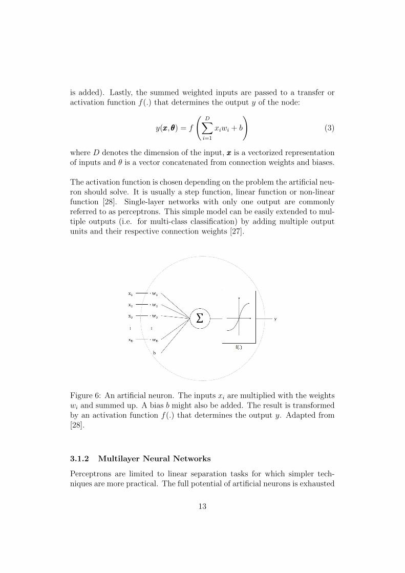
is added). Lastly, the summed weighted inputs are passed to a transfer oractivation function f(.) that determines the output y of the node:

y(xxx,θθθ) = f

(D∑i=1

xiwi + b

)(3)

where D denotes the dimension of the input, xxx is a vectorized representationof inputs and θ is a vector concatenated from connection weights and biases.

The activation function is chosen depending on the problem the artificial neu-ron should solve. It is usually a step function, linear function or non-linearfunction [28]. Single-layer networks with only one output are commonlyreferred to as perceptrons. This simple model can be easily extended to mul-tiple outputs (i.e. for multi-class classification) by adding multiple outputunits and their respective connection weights [27].

Figure 6: An artificial neuron. The inputs xi are multiplied with the weightswi and summed up. A bias b might also be added. The result is transformedby an activation function f(.) that determines the output y. Adapted from[28].

3.1.2 Multilayer Neural Networks

Perceptrons are limited to linear separation tasks for which simpler tech-niques are more practical. The full potential of artificial neurons is exhausted

13

when so-called hidden layers are introduced between the input and outputlayer. While the design of the input and output layer are usually consid-ered fixed (the number of input nodes is dependent on the dimensions of theinput and the number of output nodes determines the number of classes),the amount of hidden layers and artificial neurons in each layer is dependenton application. Hidden layers have to be designed to be able to model alluseful patterns in the input, while not over-fitting the data. Each hiddenlayer consists of several nodes that are connected to the nodes of the nextlayer in a specific way.

The most simple architecture of a multilayer network is the multilayer per-ceptron. It consists of one hidden layer and each layer is fully connectedto the next one. A graphical representation can be seen in figure 7. Itscomposition function can be written as:

y(xxx,θθθ) = f (2)

(M∑j=1

w(2)kj f

(1)

(D∑i=1

w(1)ji xi + b(1)

)+ b(2)

)(4)

where M is the number of nodes in the hidden layer and the subscript de-notes the layer number. Note that the input layer is usually not counted,making the multilayer perceptron a 2-layer neural network. A network likethe multi-layer perceptron in figure 7 is referred to as feed-forward neuralnetwork (FNN). FNNs propagate information from input to output in onlyone direction. The other main group of networks are recurrent neural net-works (RNNs) that allow for information to flow in the opposite direction.

3.1.3 Activation Functions

Usually, the same type of non-linear, sigmoidal activation function is appliedto the hidden layers. The most commonly used functions are either thelogistic sigmoid function

f(x) = σ(x) =1

1 + e−x(5)

or the hyperbolic tangent function

f(x) = tanh(x) =ex − e−x

ex + e−x(6)

A plot of these functions can be observed in figure 8. The major differencebetween these two activations is the range of output values. While the logis-tic sigmoid function results in values between [0, 1], the hyperbolic tangent

14

Figure 7: A multilayer perceptron. It has one hidden layer and all layers arefully connected, meaning that each node of a layer connects with all nodesof the next layer.

function yields values in the range of [−1, 1]. Because of its zero-centeredoutput, tanh activation functions are usually preferred [27].

(a) logistic sigmoid (b) hyperbolic tangent

Figure 8: Non-linear, sigmoidal activation functions. The logistic sigmoid in(a) maps input values to a range of [0, 1], the hyperbolic tangent function in(b) to values between [−1, 1].

For output layers, the activation function depends on the problem beingsolved. While for binary classification, sigmoidal output funcitons as seen inequations 5 and 6 are appropriate, linear activation functions are chosen for

15

regression problems. For multi-class problems, a softmax activation functionof the form

p(Ck|xxx) =eak∑j e

aj(7)

withak = ln p(x|Ck)p(Ck) (8)

is commonly used. Here, p(Ck|xxx) is the posterior probability for class Ck,p(x|Ck) are the class-conditional densities and p(Ck) are the class priors.The softmax function is the generalization of the logistic sigmoid to K > 2classes. Its name comes from the fact that it represents a smoothed version ofthe max function [29]. The outputs of a softmax funciton is the probabilityof an input xxx belonging in a class Ck, which are values between 0 and 1that add up to 1. Therefore, the output of a softmax layer can be seen as aprobability distribution.

3.1.4 Training a Neural Network

The fundamental problem in learning a neural network is the determinationof network parameters. The connection weights an biases of each node to-gether make up the parameter vector θθθ, which defines the overall behaviourof the network. Identification of the optimal parameters for a given problemcan be formulated as the minimization of an error function E(θθθ).

The error function is a measure of discrepancy between the desired outputand the actual output of the model. Its choice depends, similar to that ofthe activation function, on the type of problem being solved. For regression,a sum-of-squares error function

E(θθθ) =1

2

N∑i=1

(y(xi, θθθ)− ti)2 (9)

where N is the number of observations x1, ..., xN and t1, ..., tN are the corre-sponding target values, is used. A cross-entropy function is used for binaryclassification. It has the form

E(θθθ) = −N∑i=1

(ti ln(yi)(1 + ti) ln(1− yi)) (10)

where yi denotes y(xi, θθθ). The cross-entropy error function can be generalizedto multi-class problems with K classes using

E(θθθ) = −N∑i=1

K∑k=1

tki ln yk(xi, θθθ) (11)

16

[29].

The error function can be viewed as a surface sitting over the parameterspace defined by the vector θθθ, as seen in figure 9. It is a smooth and contin-uous, but also a non-linear, non-convex function. Therefore, the parameterset θθθ that minimizes the function can not be computed analytically, becausethe function possesses local minima besides the global minimum [27].

Therefore, computation of the minimizing parameter vector is usually doneiteratively, recalculating the parameter vector in each step:

θθθ(τ+1) = θθθ(τ) + ∆θθθ(τ) (12)

τ is the current iteration step and ∆θθθ(τ) is the update of the parameter vectorin this step.

Figure 9: Graphical interpretation ofan error function E(θ) in two dimen-sions. It can be viewed as a surfaceover the parameter space defined bythe vector θθθ. Point θθθA shows a localminimum, θθθB is the global minimum.The local gradient of the error functionis given by the vector ∇EEE and can becalculated in every point, like in θθθC .Adapted from [29].

The most common way to calculatethe update is by using gradient in-formation:

θθθ(τ+1) = θθθ(τ) − η∇E(θθθ(τ)) (13)

η is called learning rate. This pro-cedure is called gradient descent al-gorithm. The gradient of the errorfunction ∇E(θθθ) always points intothe direction of greatest rate of in-crease of the function. By movingin the opposite direction, the erroris therefore reduced. Since E(θθθ) is asmooth, continuous function, a vec-tor θθθ for which the gradient vanishesexists [27], [29]. The learning rateη is used to control the length ofeach step taken in the current direc-tion. This prevents over-correctionof the current variables, which couldlead to divergence. So to speak, thelearning rate determines how fast anetwork changes established param-eters for new ones. Often a decay function is used for the learning rate, sobig steps are taken in the beginning of the algorithm, then learning rate is

17

gradually decreased to make smaller steps.

There are two different approaches for timing the update of the parametervector. In batch gradient descent, the parameters are updated based on thegradients ∇E evaluated over the whole training set. In stochastic gradientdescent, the gradient is calculated for one sample in each iteration step andthe parameters are updated accordingly. In deep networks, stochastic gradi-ent descent is more commonly used [30].

The gradient of the error function for a network with L layers is given by

∇E(ΘΘΘ) =

[∂E

∂ΘΘΘ(1)· · · ∂E

∂ΘΘΘ(l)· · · ∂E

∂ΘΘΘ(L)

], (14)

where the superscript denotes the layer index. For the gradient descentalgorithm, this gradient needs to be calculated in every update step. Tocompute this efficiently, error backpropagation is usually used. The ideabehind error backpropagation is to propagate the resulting error from theoutput layer back to the input layer [31]. For this, a so-called error messageδ(l) is calculated for every layer 1, ..., l, ..., L. The error message of each nodecan be seen as a measure for the contribution of said node to the outputerror. Since the states and desired outputs for hidden layers are not known,error terms can not be calculated but have to be estimated by propagatingthe error messages backwards through the network. Layer l receives an errormessage δ(l+1) from layer l + 1 and updates it using

δ(l) = f ′(zzz(l)) ·[(ΘΘΘ(l+1))ᵀδ(l+1)

](15)

where zzz(l) is the input vector of layer l and f ′(.) is the inverse of the activationfunction, and passes it on to layer l− 1. Furthermore, the activation of layerl aaa(l) is used to calculate the gradient of the error function with respect tothe parameters of the current layer:

∂E(ΘΘΘ)

∂ΘΘΘ(l)= δ(l)aaa(l). (16)

This is repeated for every layer [27]. The basic concepts of error backpropa-gation are illustrated in figure 10.

3.1.5 Regularization

As already mentioned, the number of hidden units in an ANN is a parameterwhich significantly influences the performance of the network, since it also

18

Figure 10: Error backpropagation. The error message δ is propagated fromoutput to input and updated in every layer. In each layer, the partial deriva-tives with respect to the parameters ΘΘΘ(l) are calculated using the error mes-sage. Together, these partial derivatives make up the gradient of the errorfunction ∇E.

controls the number of trainable parameters. It has to be chosen to find abalance between over- and underfitting. If the number of hidden layers andparameters is to small, the model won’t work accurately. If it is too big, itwill lose its ability to generalize beyond the training data and become toospecialized [29].

The most common way to avoid overfitting is regularization. For this ap-proach, a regularization term is added to the error function. This is often aquadratic term, resulting in a regularized error function of the form

E(ΘΘΘ) = E(ΘΘΘ) +λ

2ΘΘΘᵀΘΘΘ. (17)

λ is called the regularization coefficient and can be used to model the com-plexity of the resulting network. By minimizing this regularized error func-tion, one encourages the network parameters (weights and biases) to adoptsmall values, therefore the regularization term is often referred to as weightdecay [32].

3.1.6 Convolutional Neural Networks (CNNs)

In the multi-layer networks discussed in the previous sections, inputs werein vector form and network layers were fully connected. However, this is notpractical for image data. Each pixel in the input image counts as one inputdimension. If each of these inputs were connected to a hidden layer witha few 100 hidden units, an image of size 200 ×200 would already result in

19

several 40,000 weights per neuron and over 4,000,000 weights for the wholelayer. Training all these weights would require a large amount of trainingdata and memory. Furthermore, a lot of information is gained from the topol-ogy of the input, in example local correlations among neighbouring pixels.This information is destroyed when vectorizing image data. Therefore, con-volutional layers are introduced into the network architecture. These layersforce the network to extract local features by restricting the receptive fieldsof hidden units to a certain neighbourhood of the input. Such features couldbe oriented edges, end-points or corners [33].

Figure 11: Convolution and pooling. An 8×8 image is convolved with a3×3 filter kernel to make up a feature map. For a stride of 1 and withzero padding, the feature map has the same dimensions as the input. Thefeature map is then pooled using a receptive field of size 2× and a stride of2, resulting in a 4×4 feature map. By using several different filter kernels,three-dimensional feature maps are obtained. Adapted from [29].

Each unit of a convolutional layer receives inputs from a small neighbourhoodof units in the previous layer. This neighbourhood is also called receptivefield. Sets of neurons whose receptive fields are located at different partsof the image are grouped together to have identical weight vectors (”weightsharing”). As an output, these sets produce so-called feature maps. A convo-lutional layer consists of several such unit sets, therefore, the output of theselayers is a three dimensional volume where width and height are dependenton width and height of the input, and the depth is equivalent to the numberof neuron sets in the layer. This process can also be understood as convolv-ing the input with several different filter kernels, each kernel contributing one

20

feature map to the output. The filters are defined by their values, given bythe weights of the network, and their size, defined by the size of the receptivefields. Besides the number of filters, there are two more parameters that in-fluence the size of the feature map. Firstly, the stride is the number of pixelsby which the kernel slides over the input image in each step. A larger strideresults in reduced width and height of the feature map, a stride of 1 wouldleave widht and height unchanged. Secondly, zero-padding is sometimes ap-plied to the borders of the image to allow for the application of the filter tobordering pixels. Since in convolutional layers many neurons share the sameweights, the number of parameters to train is greatly reduced. Furthermore,if the input image is shifted, the feature maps will shift in the same waybut remain otherwise unchanged. This makes the network invariant to smallshifts [33], [29].

Figure 12: Rectified Linear Unit(ReLU) activation function. It isequal to thresholding the values atzero, setting all negative values tozero.

Since convolution is a linear operation,but the data a CNN should learn ismostly non-linear, non-linearity mustbe introduced via a suitable activationfunction. Convolutional layers can usenon linear activation functions such asthe hyperbolic tangent or logistic sig-moid, but another type of activationfunction has been found to perform bet-ter, namely the Rectified Linear Unit(ReLU) function

f(x) = ReLU(x) = max(0, x), (18)

which can be seen in figure 12.

Subsequently, another new type of layer is introduced, the pooling layer. Itspurpose is to downsample an input feature map by reducing the width andheight of each map, but leaving the depth unchanged. Similar to the convo-lution layer, each unit of the pooling layer is connected to a receptive field ofunits from the previous layer. There are several variants for pooling, such asmax pooling where the maximal value inside a receptive field is taken, or av-erage or mean pooling, where the average/mean value is calculated. Poolinghas the purpose of decreasing the feature dimensions and therefore, furtherreduce the number of parameters (weights, biases) of the network. Further-more, it makes the network invariant to small scaling. Image 11 shows anillustration of convolving and pooling layers applied to an input image [27].

21

In a convolutional neural networks, several convolutional and pooling layerscan be applied successively. The deeper the network becomes (the morehidden layers it has), the better the ability of the network to extract usefulfeatures. The outputs of such a network are high level, low dimensionalfeatures of the input that finally have to be classified. Fully connected layerswith appropriate activation functions, as discussed in the previous sections,are usually used for this task. A typical neural network architecture can beseen in figure 13

Figure 13: Convolutional neural network with two convolution and poolinglayers. The input image of dimension 8×8 is convolved with three kernelsto produce a 3×8×8 feature map. Width and height are reduced in the firstpooling layer to the dimension 3×4×4. The feature map is then convolvedand pooled for a second time in the same manner. The output layer is fullyconnected and produces a vector of 24×1×1. Adapted from [33].

3.2 Medical Image Segmentation

Segmentation is the process of subdividing an image in its constituent re-gions or objects. For non-trivial, natural images, automatic segmentation isone of the most challenging tasks in image processing. Since segmentation isoften the first step in computerized image analysis algorithms, it’s accuracyis determining the success of subsequent steps. Therefore, segmentation al-gorithms must be very precise. Generally, there are two basic approaches toautomatic image segmentation:

1. Discontinuity-based approaches aim to find sharp, local changes of in-tensities in images, such as edges, and partition the image based onthose discontinuities.

22

2. Similarity-based approaches partition an image into regions that aresimilar according to a pre-defined criterion. Intensity is a criterionthat is most often used, but other characteristics like colour or texturemight be used as well [34].

In medical image processing, segmentation plays an important role in manyapplications, such as the quantification of tissue volumes, the study of anatom-ical structures, the localization of pathologies, treatment planning (especiallyradiotherapy planning), computer-integrated surgery and computer aided di-agnosis.

3.2.1 Common Segmentation Methods in Medical Imaging

Medical image data is very hard to segment automatically due to its com-plexity. Anatomical structures usually have a large variability in shape andlocation, and medical images are prone to artefacts and noise, furthermoretheir resolution is often limited. Therefore, in clinical practise, segmentationis mostly done manually or semi-manually. Manual segmentation is usuallyperformed by one or more physicians who delineate regions of interest sliceby slice using simple drawing tools. This process obviously has many short-comings: First of all, the workload for individual physicians is huge sincedelineation is very time consuming, which in turn leads to errors. Further-more, results are not reproducible. This, as well as the growing size andnumber of medical image data, has led to the increasing importance of auto-matic segmentation algorithms for the delineation of anatomical structuresor other regions of interest.The following section provides an overview over common medical image seg-mentation methods found in recent literature and is adapted from [1], whichthe reader might refer to for in-depth information.

• ThresholdingThresholding based methods create a binary partitioning of the imagebased on intensity values. In the thresholding procedure, the inten-sity histogram of an image is usually used to find an intensity valuethat best separates the desired classes from one another. This value iscalled the threshold. An example for this can be seen in figure 14(a).Subsequently, all pixels with intensity values below the threshold aregrouped to one class (frequently labelled background) and the remain-ing pixels belong to the object. Thresholding is widely used due to itssimplicity, however, it requires structures to have distinct contrastingintensities. Furthermore, it does not take spatial information into ac-count, which makes it sensitive to noise and intensity inhomogeneities

23

which are often present in medical image data. Therefore, thresholdingis seldom used alone. It is, however, often used as an initial step forfurther processing operations.

• Region GrowingRegion growing methods, in their simplest form, usually start froma seed point inside a region of interest, and then progressively includeneighbouring pixels which satisfy a predefined similarity criterion. Usu-ally, a fixed interval around a certain intensity is chosen as a criterion,which makes this approach similar to thresholding, but with the consid-eration of spatial information. Region growing is also most commonlyused within a more complex segmentation pipeline. One disadvantageof region growing is that, in general, user input in form of a seed pointis required for every region to extract.

• Classifiers and ClusteringClassifier algorithms assign a certain label to an image or an imagepatch. For this, the classifier must be trained using image data withknown labels. Usually, multidimensional features, which are abstract,reduced representations of images (i.e. edge directions), are calculated.Then the classifier is chosen in a way that best separates the featurespace into the desired categories. This can be seen in figure 14(b). Theclassifier can then be used to decide in which category a new image orimage patch belongs. A downside of classifiers is, that they use handcrafted features. This means that the user must decide which type offeatures best represent the information he wants to extract to obtainthe best results.Clustering algorithms are very similar in their functionality to classi-fier methods, but they do not require training data. These algorithmsgroup similar instances together, based on previously extracted fea-tures. Clustering methods, however, can’t assign predefined labels tothese groups.

• Deformable ModelsDeformable models use parametric curves or surfaces that are deformedby internal or external influences. For this, an initial model is placednear the boundary one wants to delineate. Then external influencesdrive the model towards the desired boundary, while internal con-straints ensure that the model stays smooth.

24

(a)

(b)

Figure 14: Graphical interpretation of thresholding and classification. (a)Finding a threshold based on the image histogram. The threshold T is chosenin a way that best separates the intensity values in an image. (b) Seperatinga 2D-feature space with a linear classifier. First, features with known labels(circles, triangles) are seperated. This classifier can then be used to assignunlabelled objects to one of the two classes.

3.2.2 Deep Learning Artificial Neural Networks for Image Seg-mentation

Deep learning algorithms using ANNs have made a large impact on the fieldof automatic image analysis in the past years, outperforming state of the artmethods in many visual recognition tasks. They possess various advantagesover the established methods discussed before. Deep learning approachesdon’t require user interaction, like a seed point in region growing or a initialmodel like with deformable models. Furthermore, contrary to classifiers orclustering, no hand crafted features are needed. Deep ANNs learn multiplelayers of representation. Input data can be represented in many ways, butcertain representations are better suited to learn a task of interest (e.g. clas-sification). Deep learning algorithms attempt to find the best representationof images by learning complex relationships amongst the input data. Usually,many layers of non-linear data processing are used in the course of this [35].

Convolutional neural networks are commonly used for classification tasks,where input data (e.g. an image) is assigned to a single class label. How-ever, in many recognition tasks, especially in biomedical imaging, localizationshould be considered in the output, i.e. a label prediction should be madeat every pixel. The CNNs as discussed in chapter 3.1 are not applicableon semantic segmentation since they produce low dimensional, non spacial

25

feature maps which don’t allow pixel-wise labelling. An early idea to transi-tion from classification to segmentation was to classify each pixel based on apatch around that pixel [36]. However, this approach is rather slow and has atrade-off between localization accuracy and context depending on the patchsize [37]. A better solution to this problem is the application of fully convo-lutional neural networks (FCNs) as proposed by Long et al. in [38]. Thesenetworks take an arbitrary sized input and produce a segmented output ofcorresponding size. Contrary to traditional classification networks, FCNsuse only convolution and pooling layers combined with non-linear activationfunctions, and no fully connected layers. FCNs will be discussed in greaterdetail in section 4.2. A further development in semantic segmentation usingCNNs is the Encoder-Decoder Convolutional Neural Network (ED-CNN),like SegNet in [39] or U-Net in [37]. In an ED-CNN, the contracting path(encoder) is followed by a expansive path (decoder) that performs upsam-pling in many steps, using the stored pooling indices. This way, contextinformation is propagated to higher resolution layers. Both paths are moreor less symmetric, yielding a u- or v-shaped architecture. Higher level fea-tures from the encoder path can be combined with upsampled outputs fromthe decoder path to produce a more precise result.

3.3 MeVisLab

The following section follows my masters’ project report in [18] and is adaptedfrom the MeVisLab Getting Started Guide [40], the MeVisLab ReferenceManual [41] as well as [42] and [43].

MeVisLab is a modular framework for the development of medical imageprocessing algorithms and visualization of medical data. The framework of-fers a wide range of features, from basic image processing algorithms likefilters and transformations, to more advanced medical imaging modules, inexample for segmentation or registration. Development can be done on threelevels. A visual level using graphical programming enables the creation ofimage processing networks via the inclusion of processing, visualization andinteraction modules. On a scripting level, macro modules can be createdusing Python scripting to control interactions between network modules, thegraphical user interface (GUI) and internal parameters. Lastly, new modulescan be programmed and integrated using the C++ class library. Further-more, the MeVisLab Definition Language (MDL) allows the design of GUIs.Visual programming and setting up macro modules will be explained in moredetail in the following sections. Since module programming in C++ was notpart of this project, no further information will be provided about it.

26

3.3.1 Visual Programming

Visual programming using modules integrated in the MeVisLab frameworkand connections between modules is the most basic form of implementingalgorithms in MeVisLab. Three basic module types distinguished by theircolors, are available. They are shown in figure 15. Blue modules representalgorithms from the MeVis Image Processing Library (ML). They containpage-based, demand-driven processing functions. Open Inventor modules (ingreen) provide visual, three dimensional scene graphs or scene objects. Fi-nally, a brown color indicates macro modules, which represent a combinationof other module types, connected by a specific hierarchy and scripted inter-actions. Most modules have connectors, the bottom ones indicating moduleinputs and the top ones module outputs.

Figure 15: Basic module types and module connectors of MeVisLab. Ablue color indicates ML modules, green modules are Open Inventor modulesand a brown color marks macro modules. Connectors can have the form oftriangles (ML images), half circles (Open Inventor scenes) or rectangles (datastructure pointers).

Modules can be connected in two basic ways. By connecting the moduleconnectors, image data or Open Inventor information is transported betweenmodules. Each connector shape defines a certain type: Triangles indicate thetransportation of ML images, half circles of Inventor scenes and squares ofpointers to data structures. These connector types can also be seen in figure15. The second way to connect modules is via parameter connection. Withthis, any field of a module can be connected to a compatible field. This allows,for example, the synchronization of parameters between different modules.Figure 16 shows an example for a fully connected network in MeVisLab.ML, Open Inventor and macro modules are used. Data connections as wellas parameter connections are shown.

3.3.2 Creation of Macro Modules

A macro module is a combination of several other modules that allows theimplementation of hierarchies and scripted interactions between modules. To

27

Figure 16: Example network in MeVisLab. All three types of modules areused. Blue and green lines indicate connetions between module connectors(data connections), grey arrows indicate parameter connections.

implement a macro module in MeVisLab, several files are necessary:

1. The module definition file (*.def). This file contains some generalinformation about the module, like name, author and date of creation.It is also possible to define a genre and keywords of the module to makeit easier to find for other users.

2. The MeVisLab Definition Language (MDL) script file (*.script). Thisfile defines the interface of the module, like input-, output- and param-eter fields. Furthermore, the graphical user interface (GUI) can bemanipulated here.

3. The Python script files (*.py). Here, functions and interactions be-tween modules can be implemented using Python scripting.

4. The internal network (*.mlab). This file contains the internal networkstructure of the macro module.

For creating macro modules, MeVisLab provides a tool named Project Wiz-ard, which sets up all required files and their connections.

28

3.4 TensorFlow

TensorFlow is a platform independent open-source software library for nu-merical computation, mostly used for machine learning. It is both an in-terface for expressing machine learning algorithms, as well as an implemen-tation for executing these algorithms. This section explains basic conceptsof TensorFlow and is adapted from the TensorFlow whitepaper [44] and theTensorFlow developement guide [45].

3.4.1 Tensors

All data within a TensorFlow program is represented as a tensor, as the namesuggests. Tensors can be thought of as multi-dimensional arrays or lists thatare passed between operations. A tensor is characterized by its rank, whichdescribes the dimensionality of the tensor, its shape and its data type, e.g.signed or unsigned integer types, IEEE float and double types or string type.

3.4.2 Computation Graphs and Sessions

In TensorFlow, programs are divided into two phases:

1. The construction phase

2. The execution phase

In the construction phase, a computation graph is assembled. The nodesof the graph represent operations, and information is passed between nodesalong the edges of the graph in the form of tensors. Operations are abstractcomputations, in example ”add” or ”matrix multiply”. Usually, computa-tion graphs are started using operations that don’t require inputs, e.g. atf.constant:

1 const1 = tf.constant (3.0, dtype = tf.float)

2 const2 = tf.constant (4.0, dtype = tf.float)

3 print(const1 , const2)

which would produce the output

Tensor("Const :0", shape =(), dtype=float32) Tensor("Const_1 :0", shape =(),

dtype=float32)

It can be seen from this simple example, that constant1 is not an actualvalue, but a node that outputs a tensor. It is important to note that acomputation graph doesn’t compute anything, but is rather a descriptionof computations and operations. Computations are done in the executionphase by launching the graph in a session. Within the session, the graph istranslated to executable operations which can be distributed across different

29

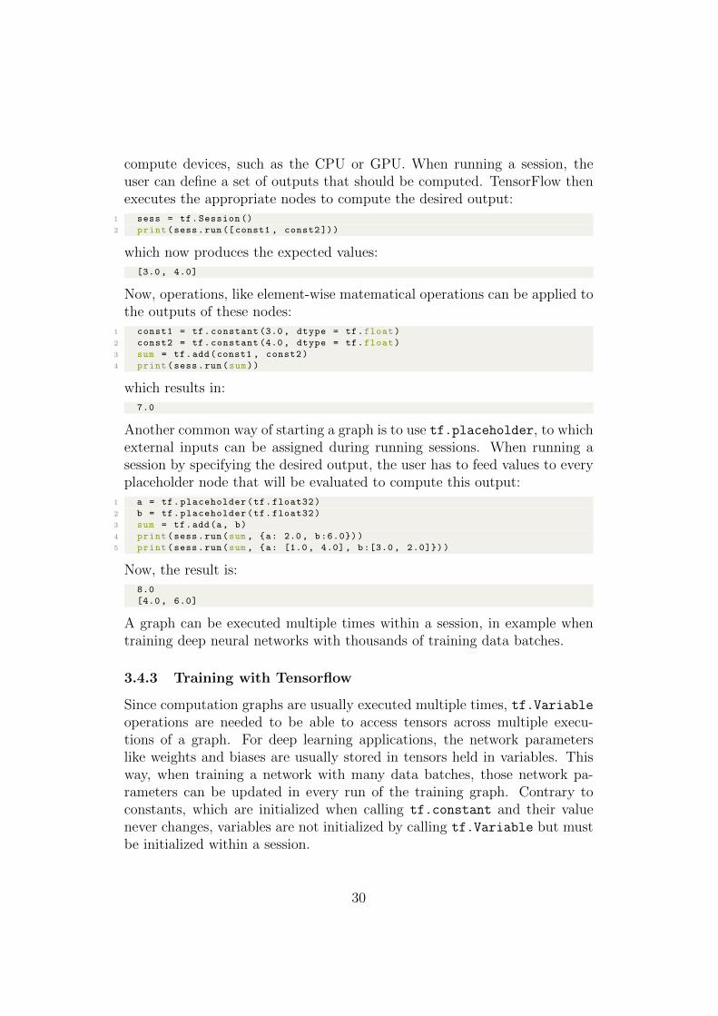
compute devices, such as the CPU or GPU. When running a session, theuser can define a set of outputs that should be computed. TensorFlow thenexecutes the appropriate nodes to compute the desired output:

1 sess = tf.Session ()

2 print(sess.run([const1 , const2 ]))

which now produces the expected values:[3.0, 4.0]

Now, operations, like element-wise matematical operations can be applied tothe outputs of these nodes:

1 const1 = tf.constant (3.0, dtype = tf.float)

2 const2 = tf.constant (4.0, dtype = tf.float)

3 sum = tf.add(const1 , const2)

4 print(sess.run(sum))

which results in:7.0

Another common way of starting a graph is to use tf.placeholder, to whichexternal inputs can be assigned during running sessions. When running asession by specifying the desired output, the user has to feed values to everyplaceholder node that will be evaluated to compute this output:

1 a = tf.placeholder(tf.float32)

2 b = tf.placeholder(tf.float32)

3 sum = tf.add(a, b)

4 print(sess.run(sum , {a: 2.0, b:6.0}))

5 print(sess.run(sum , {a: [1.0, 4.0], b:[3.0, 2.0]}))

Now, the result is:8.0

[4.0, 6.0]

A graph can be executed multiple times within a session, in example whentraining deep neural networks with thousands of training data batches.

3.4.3 Training with Tensorflow

Since computation graphs are usually executed multiple times, tf.Variableoperations are needed to be able to access tensors across multiple execu-tions of a graph. For deep learning applications, the network parameterslike weights and biases are usually stored in tensors held in variables. Thisway, when training a network with many data batches, those network pa-rameters can be updated in every run of the training graph. Contrary toconstants, which are initialized when calling tf.constant and their valuenever changes, variables are not initialized by calling tf.Variable but mustbe initialized within a session.

30

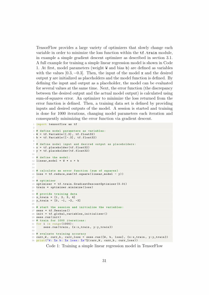
TensorFlow provides a large variety of optimizers that slowly change eachvariable in order to minimize the loss function within the tf.train module,in example a simple gradient descent optimizer as described in section 3.1.A full example for training a simple linear regression model is shown in Code1. At first, model parameters (weight W and bias b) are defined as variableswith the values [0.3,−0.3]. Then, the input of the model x and the desiredoutput y are initialized as placeholders and the model function is defined. Bydefining the input and output as a placeholder, the model can be evaluatedfor several values at the same time. Next, the error function (the discrepancybetween the desired output and the actual model output) is calculated usingsum-of-squares error. An optimizer to minimize the loss returned from theerror function is defined. Then, a training data set is defined by providinginputs and desired outputs of the model. A session is started and trainingis done for 1000 iterations, changing model parameters each iteration andconsequently minimizing the error function via gradient descent.

1 import tensorflow as tf

2

3 # define model parameters as variables:

4 W = tf.Variable ([.3], tf.float32)

5 b = tf.Variable ([-.3], tf.float32)

6

7 # define model input and desired output as placeholders:

8 x = tf.placeholder(tf.float32)

9 y = tf.placeholder(tf.float32)

10

11 # define the model:

12 linear_model = W * x + b

13

14

15 # calculate an error function (sum of squares)

16 loss = tf.reduce_sum(tf.square(linear_model - y))

17

18 # optimizer

19 optimizer = tf.train.GradientDescentOptimizer (0.01)

20 train = optimizer.minimize(loss)

21

22 # provide training data

23 x_train = [1, 2, 3, 4]

24 y_train = [0, -1, -2, -3]

25

26 # start the session and initialize the variables:

27 sess = tf.Session ()

28 init = tf.global_variables_initializer ()

29 sess.run(init)

30 # train for 1000 iterations:

31 for i in range (1000):

32 sess.run(train , {x:x_train , y:y_train })

33

34 # evaluate training accuracy

35 curr_W , curr_b , curr_loss = sess.run([W, b, loss], {x:x_train , y:y_train })

36 print("W: %s b: %s loss: %s"%(curr_W , curr_b , curr_loss))

Code 1: Training a simple linear regression model in TensorFlow

31

Running this program displays the final model parameters as well as the finalloss:

W: [ -0.9999969] b: [ 0.99999082] loss: 5.69997e-11

3.4.4 TensorBoard

TensorBoard is suite of visualization tools for inspecting and understandingTensorFlow graphs and sessions. It is designed to enable easier understand-ing, debugging and optimization of TensorFlow programs.

TensorBoard requires a log file, called a summary, from which it reads data tovisualize. While creating the TensorFlow graph, the user can annotate nodeswith summary operations which will export information about the node theyare attached to. Like any other node, a summary operation needs to be runwithin a session to actually generate data. The collected summary data canthen be written to a log directory, from which TensorBoard acquires all theinformation it needs for visualization. A popular application for TensorBoardis to monitor the development of the loss during training. For the linearregression model above, a summary node can be added with the followingline:

tf.summary.scalar(’sum_of_squared_differences ’, loss)

Then, all summary nodes are merged and a summary file writer is defined:

merged = tf.summary.merge_all ()

train_writer = tf.summary.FileWriter("path/to/log/folder", sess.graph)

and within the session, this file writer is run:

for i in range (1000):

sess.run(train , {x:x_train , y:y_train })

summary = sess.run(merged , {x:x_train , y:y_train })

train_writer.add_summary(summary , i)

Now, a log file will be created in the specified folder. When opening this filewith TensorBoard, the progress of loss during training can be observed andmanipulated using different visualization tools, as seen in figure 17.

TensorBoard also enables the visual inspection of the constructed graphs bydisplaying all operation nodes and how tensors are passed between them.The example for the linear regression model graph in figure 18 (a) shows,that even for simple models those graphs contain numerous nodes, makingvisualization confusing. Therefore, TensorFlow allows to name nodes, and toscope nodes together, defining a hierarchy in the graph. Figure 18 (b) showsa graph of the same linear regression model, but this time, nodes are namedand grouped together using name scopes.

32

Figure 17: Visualization of the development of sum-of-squares error duringtraining a linear regression model in TensorBoard. Development is shown for1000 training iterations. It can be seen how the error quickly decreases withevery iteration.

(a) Unedited Graph of a linear regressionmodel (b) Graph of a linear regression model,

structured by using name scopes andnamed nodes

Figure 18: Graph visualization in TensorBoard. Image (a) shows an uneditedgraph, which can get confusing quickly. (b) shows the same graph, structuredusing name scopes and with some named nodes, which makes understandingthe graph easier. Nodes in one name scope are displayed collapsed, but scopescan be expanded to reveal their inner structure, like the sum of squareddifferences error scope in this example.

33

3.4.5 TensorFlow-Slim

TensorFlow-Slim (TF-Slim) is a high-level library for defining, training andevaluating complex models in TensorFlow. It is designed to make program-ming with TensorFlow simpler and to improve the readability of code by

• the usage of argument scoping, allowing the user to define default ar-guments for specific operations, reducing repetitive code,

• providing high level functions for defining layers, variables, regularizers,losses etc,

• providing network definitions for popular computer vision models, e.g.VGG-Net or ResNet, including pre-trained parameters in the form ofmodel checkpoints.

Since TensorFlow is very low-level, defining complex models can result incomplicated scripts with a lot of boilerplate code. TF-Slim offers an easyway around this and can also be mixed with native TensorFlow and otherTensorFlow frameworks.

34

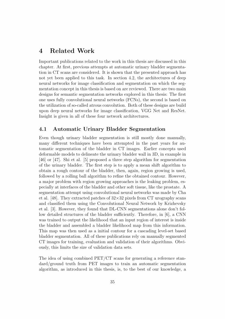
4 Related Work

Important publications related to the work in this thesis are discussed in thischapter. At first, previous attempts at automatic urinary bladder segmenta-tion in CT scans are considered. It is shown that the presented approach hasnot yet been applied to this task. In section 4.2, the architectures of deepneural networks for image classification and segmentation on which the seg-mentation concept in this thesis is based on are reviewed. There are two maindesigns for semantic segmentation networks explored in this thesis: The firstone uses fully convolutional neural networks (FCNs), the second is based onthe utilization of so-called atrous convolution. Both of these designs are buildupon deep neural networks for image classification, VGG Net and ResNet.Insight is given in all of these four network architectures.

4.1 Automatic Urinary Bladder Segmentation

Even though urinary bladder segmentation is still mostly done manually,many different techniques have been attempted in the past years for au-tomatic segmentation of the bladder in CT images. Earlier concepts useddeformable models to delineate the urinary bladder wall in 3D, in example in[46] or [47]. Shi et al. [5] proposed a three step algorithm for segmentationof the urinary bladder. The first step is to apply a mean shift algorithm toobtain a rough contour of the bladder, then, again, region growing is used,followed by a rolling ball algorithm to refine the obtained contour. However,a major problem with region growing approaches is the leaking problem, es-pecially at interfaces of the bladder and other soft tissue, like the prostate. Asegmentation attempt using convolutional neural networks was made by Chaet al. [48]. They extracted patches of 32×32 pixels from CT urography scansand classified them using the Convolutional Neural Network by Krizhevskyet al. [3]. However, they found that DL-CNN segmentations alone don’t fol-low detailed structures of the bladder sufficiently. Therefore, in [6], a CNNwas trained to output the likelihood that an input region of interest is insidethe bladder and assembled a bladder likelihood map from this information.This map was then used as a initial contour for a cascading level-set basedbladder segmentation. All of these publications rely on manually segmentedCT images for training, evaluation and validation of their algorithms. Obvi-ously, this limits the size of validation data sets.

The idea of using combined PET/CT scans for generating a reference stan-dard/ground truth from PET images to train an automatic segmentationalgorithm, as introduced in this thesis, is, to the best of our knowledge, a

35

new approach. Furthermore, advanced deep learning techniques for semanticsegmentation, relying on fully convolutional neural networks and upsamplingof coarse feature maps instead of patch-wise classification, have not yet beenapplied to the problem of urinary bladder segmentation in CT images, as faras we know.

4.2 Neural Networks for Image Classification and Seg-mentation

4.2.1 VGG Classification Network

Figure 19: VGG 16 architecture. The network consists of five convolutionblocks, each containing several convolutions, and followed by a max poolinglayer. After the stack of convolutional layers, three fully connected layers areapplied. The last layer uses a softmax activation function to map the outputof the network to probabilities.

The very deep convolutional networks for large-scale image recognition [49],developed by the Visual Geometry Group of the University of Oxford (hence,the short term VGG-Net) were a runner-up in ImageNet Large Scale VisualRecognition Competition (ILSVRC) 2014 and have since then been used forvarious tasks such as object detection and image segmentation. The CNNis trained on fixed-size 224×224 RGB images. Convolution layers use filterswith a kernel size of 3×3 and a stride and pad of one pixel. Therefore, thespatial resolution of a convolution layer input is preserved after the convolu-tion. Pooling is carried out by max-pooling layers over a 2×2 pixel window,

36

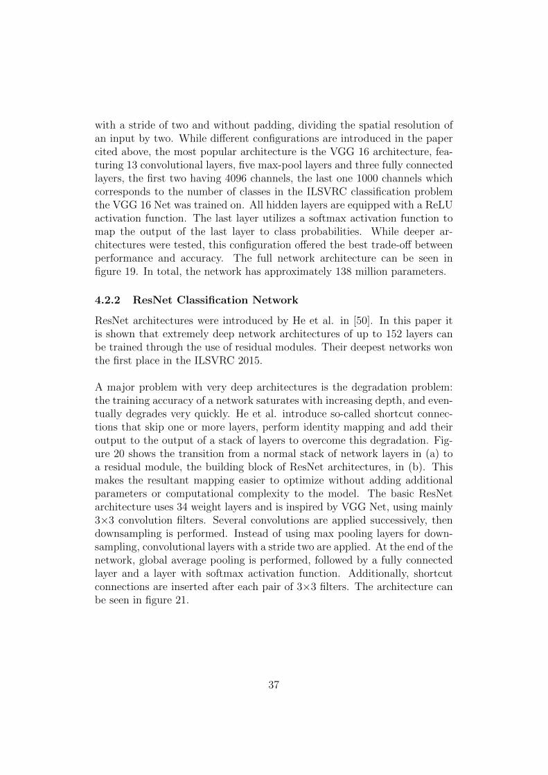
with a stride of two and without padding, dividing the spatial resolution ofan input by two. While different configurations are introduced in the papercited above, the most popular architecture is the VGG 16 architecture, fea-turing 13 convolutional layers, five max-pool layers and three fully connectedlayers, the first two having 4096 channels, the last one 1000 channels whichcorresponds to the number of classes in the ILSVRC classification problemthe VGG 16 Net was trained on. All hidden layers are equipped with a ReLUactivation function. The last layer utilizes a softmax activation function tomap the output of the last layer to class probabilities. While deeper ar-chitectures were tested, this configuration offered the best trade-off betweenperformance and accuracy. The full network architecture can be seen infigure 19. In total, the network has approximately 138 million parameters.

4.2.2 ResNet Classification Network

ResNet architectures were introduced by He et al. in [50]. In this paper itis shown that extremely deep network architectures of up to 152 layers canbe trained through the use of residual modules. Their deepest networks wonthe first place in the ILSVRC 2015.

A major problem with very deep architectures is the degradation problem:the training accuracy of a network saturates with increasing depth, and even-tually degrades very quickly. He et al. introduce so-called shortcut connec-tions that skip one or more layers, perform identity mapping and add theiroutput to the output of a stack of layers to overcome this degradation. Fig-ure 20 shows the transition from a normal stack of network layers in (a) toa residual module, the building block of ResNet architectures, in (b). Thismakes the resultant mapping easier to optimize without adding additionalparameters or computational complexity to the model. The basic ResNetarchitecture uses 34 weight layers and is inspired by VGG Net, using mainly3×3 convolution filters. Several convolutions are applied successively, thendownsampling is performed. Instead of using max pooling layers for down-sampling, convolutional layers with a stride two are applied. At the end of thenetwork, global average pooling is performed, followed by a fully connectedlayer and a layer with softmax activation function. Additionally, shortcutconnections are inserted after each pair of 3×3 filters. The architecture canbe seen in figure 21.

37

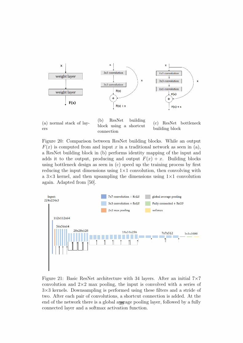
(a) normal stack of lay-ers

(b) ResNet buildingblock using a shortcutconnection

(c) ResNet bottleneckbuilding block

Figure 20: Comparison between ResNet building blocks. While an outputF (x) is computed from and input x in a traditional network as seen in (a),a ResNet building block in (b) performs identity mapping of the input andadds it to the output, producing and output F (x) + x. Building blocksusing bottleneck design as seen in (c) speed up the training process by firstreducing the input dimensions using 1×1 convolution, then convolving witha 3×3 kernel, and then upsampling the dimensions using 1×1 convolutionagain. Adapted from [50].

Figure 21: Basic ResNet architecture with 34 layers. After an initial 7×7convolution and 2×2 max pooling, the input is convolved with a series of3×3 kernels. Downsampling is performed using these filters and a stride oftwo. After each pair of convolutions, a shortcut connection is added. At theend of the network there is a global average pooling layer, followed by a fullyconnected layer and a softmax activation function.

38

To implement even deeper networks, building blocks are modified to a bot-tleneck design for faster training. This design uses three layers instead oftwo, where the dimension of the input is first reduced by a 1×1 convolution,then convolved with a 3×3 kernel, and then dimensions are restored with an-other 1×1 convolution. This building block can be seen in figure 20 (c). Thebest performing ResNet uses 152 layers, grouped together in such three-layerbottleneck blocks.

4.2.3 Fully Convolutional Networks for Semantic Segmentation(FCNs)

The FCNs introduced by Long et al. in [38] made a large impact on seman-tic segmentation with neural networks by providing end-to-end, pixel-to-pixelsegmentation networks. The basic idea behind this approach is to transformestablished classification networks to fully convolutional networks, suitablefor semantic segmentation. They achieved best results with the VGG 16 net-work. For this, fully connected layers are transformed into convolution layers,which allows the network to output a spacial heatmap. This is illusrated infigure 22. However, these output maps are considerably downsampled fromthe input image because of pooling layers, making the output very coarse. Itcan be seen from figure 19, that in case of VGG 16 Net, an input image isdownsampled by a factor of 32 after the last max pooling layer.

Figure 22: Transition from image classification to image segmentation inCNNs. In the classification network, the last layer is fully connected, in thesegmentation network, this layer is transformed to an additional convolu-tional layer. This enables the network to output a heatmap for the object ofinterest. Adapted from [38].

39

To map these coarse outputs to dense predictions, learnable upsampling lay-ers, which resample the image to its original size, are proposed. For up-sampling, not only the features from the last downsampling layer are used.Instead, so-called skip connections are introduced to use convolutional fea-tures from different layers in the network, which have different scales. Sinceshallower layers produce bigger feature maps where more spatial informationis preserved, this helps capturing finer details from the original image. Up-sampling layers are learned for each of these skip connections individually.The approach from Long et al. resulted in three network architectures. Thebasic FCN 32s architecture simply upsamples the feature map obtained fromthe adapted VGG 16 network by a factor of 32. For the FCN 16s architec-ture, the two times upsampled VGG 16 feature map is combined with thefeatures from the fourth pooling layer of VGG 16 and then upsampled byfactor 16. The best performing architecture is their FCN 8s architecture,where the combination of upsampled VGG 16 features and fourth poolinglayer results is combined with features obtained from the third pooling layerof VGG 16 and then upsampled by a factor of eight. An illustration of thesearchitectures can be seen in figure 23.

Figure 23: FCN architectures. The input image is downsampled by maxpooling layers, getting coarser from layer to layer. In the FCN 32s, theoutput of the last pooling layer is upsampled by factor 32 in a single step.In FCN 16s, features from the last layer and pool4 layer are combined andthen upsampled by factor 16. For FCN 8s, predictions from pool3 layer areinlcuded. Adapted from [38].

40

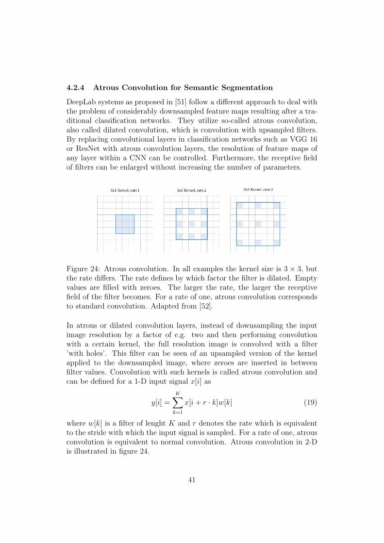
4.2.4 Atrous Convolution for Semantic Segmentation

DeepLab systems as proposed in [51] follow a different approach to deal withthe problem of considerably downsampled feature maps resulting after a tra-ditional classification networks. They utilize so-called atrous convolution,also called dilated convolution, which is convolution with upsampled filters.By replacing convolutional layers in classification networks such as VGG 16or ResNet with atrous convolution layers, the resolution of feature maps ofany layer within a CNN can be controlled. Furthermore, the receptive fieldof filters can be enlarged without increasing the number of parameters.

Figure 24: Atrous convolution. In all examples the kernel size is 3 × 3, butthe rate differs. The rate defines by which factor the filter is dilated. Emptyvalues are filled with zeroes. The larger the rate, the larger the receptivefield of the filter becomes. For a rate of one, atrous convolution correspondsto standard convolution. Adapted from [52].

In atrous or dilated convolution layers, instead of downsampling the inputimage resolution by a factor of e.g. two and then performing convolutionwith a certain kernel, the full resolution image is convolved with a filter’with holes’. This filter can be seen of an upsampled version of the kernelapplied to the downsampled image, where zeroes are inserted in betweenfilter values. Convolution with such kernels is called atrous convolution andcan be defined for a 1-D input signal x[i] as

y[i] =K∑k=1

x[i+ r · k]w[k] (19)

where w[k] is a filter of lenght K and r denotes the rate which is equivalentto the stride with which the input signal is sampled. For a rate of one, atrousconvolution is equivalent to normal convolution. Atrous convolution in 2-Dis illustrated in figure 24.

41

This convolution allows the construction of many layered networks withoutdecreasing resolution, and since only non-zero values have to be accountedfor in convolutions, the number of filter parameters does not increase. How-ever, computing feature maps at the original image resolution is not veryefficient, therefore, hybrid approaches are mostly used. Atrous convolutionlayers are applied in a way to downsample the original image by a factor ofeight in total (compared to a factor of 32 in VGG Nets or ResNets), followedby bilinear interpolation to recover feature maps of the original image res-olution. Compared to approaches using fractionally strided convolution forupsampling, no new parameters are learned within the network, which leadsto faster training.

42

5 Methods

This chapter discusses the methods with which underlying ideas were set intopractice. The first section describes the used Reference Image Database toEvaluate Therapy Response as well as the image data obtained from it. Sec-tion 5.2 explains how suitable training and testing data was generated fromthis image data using a macro module implemented in MeVisLab. The macromodule generates ground truth labels from PET image data and applies dataaugmentation. The implementation of deep neural networks for image seg-mentation using the TensorFlow library under Python is outlined in section5.3. At first, the TensorFlow-own file format TFRecords, and how it is usedto process input data efficiently, is introduced. Next, the implemented seg-mentation network architectures are described, which were created using theTF-Slim library and pre-trained classification networks. Lastly, the processof training, testing and evaluating these networks is demonstrated.

5.1 Dataset and Preprocessing

The implemented methods were trained and tested on the Reference ImageDatabase to Evaluate Therapy Response (RIDER) [53]. RIDER is a col-lection of Computed Tomography, Magnetic Resonance Imaging (MRI) andPET/CT data.

The RIDER PET/CT dataset provides serial patient studies (without meta-data) as well as data from multi-vendor and multi-parameter calibrationphantoms. It consists of de-identified Digital Imaging and Communicationsin Medicine (DICOM) serial PET/CT lung cancer patient data and pro-vides serial scans of 28 lung cancer patients (a total of 65 scans), as well asdata from studies with a long half-life calibration phantom. As radiotracer,fluorine-18-labelled fluorodeoxyglucose was used in all PET scans. The pub-lic database can be downloaded from the National Cancer Imaging Archive(NCIA) at [54].

To obtain an overview of the database, the DICOM datasets were loadedinto the medical image visualization software 3DSlicer [55]. For each patient,several CT and PET scans with different scanning and visualization param-eters are available. For this project, CT scans with a resolution of 512×512and a slice thickness of 2.5 mm were selected. The chosen PET scans have aresolution of 128×128 pixel and a slice thickness of 3.27 mm, and use stan-dardized uptake values to measure radiotracer uptake. Patient data withvery high noise levels in either the CT or PET data or with unusually low

43

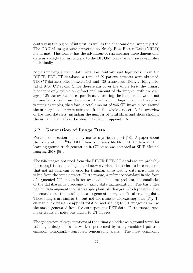
contrast in the region of interest, as well as the phantom data, were rejected.The DICOM images were converted to Nearly Raw Raster Data (NRRD)file format. This format has the advantage of representing three dimensionaldata in a single file, in contrary to the DICOM format which saves each sliceindividually.

After removing patient data with low contrast and high noise from theRIDER PET/CT database, a total of 29 patient datasets were obtained.The CT datasets offer between 148 and 358 transversal slices, yielding a to-tal of 8754 CT scans. Since these scans cover the whole torso the urinarybladder is only visible on a fractional amount of the images, with an aver-age of 25 transversal slices per dataset covering the bladder. It would notbe sensible to train our deep network with such a large amount of negativetraining examples, therefore, a total amount of 845 CT image slices aroundthe urinary bladder were extracted from the whole dataset. A full overviewof the used datasets, including the number of total slices and slices showingthe urinary bladder can be seen in table 6 in appendix A.

5.2 Generation of Image Data

Parts of this section follow my master’s project report [18]. A paper aboutthe exploitation of 18F-FDG enhanced urinary bladder in PET data for deeplearning ground truth generation in CT scans was accepted at SPIE MedicalImaging 2018 [56].

The 845 images obtained from the RIDER PET/CT database are probablynot enough to train a deep neural network with. It also has to be consideredthat not all data can be used for training, since testing data must also betaken from the same dataset. Furthermore, a reference standard in the formof segmented CT images is not available. The first problem, the small sizeof the databases, is overcome by using data augmentation. The basic ideabehind data augmentation is to apply plausible changes, which preserve labelinformation, to the existing data to generate new, additional training data.These images are similar to, but not the same as the existing data [57]. Toenlarge our dataset we applied rotation and scaling to CT images as well asthe masks generated from the corresponding PET data. Furthermore, zero-mean Gaussian noise was added to CT images.

The generation of segmentations of the urinary bladder as a ground truth fortraining a deep neural network is performed by using combined positronemission tomography-computed tomography scans. The most commonly

44

used radiotracer, 18F-FDG, accumulates in the urinary bladder, therefore,the bladder always shows up in these PET scans. Contrary to CT, PETimages exhibit high contrast and are therefore comparably easy to segmentautomatically. We automatically segment PET images using a simple thresh-olding approach to generate binary masks of the urinary bladder that matchCT data acquired from the same patients at the same time.

At first, the available 29 patient datasets containing a total of 845 imageslices showing the urinary bladder were split into training and testing data.A standard for this split commonly found in literature is 80% training data,20% testing data. Loosely following this guideline, 630 images were used fortraining and 215 images were reserved for testing, corresponding to 21 and8 patient datasets, respectively. Next, the 21 patient datasets for trainingwere processed with the proposed MeVisLab network to obtain individual,augmented CT slices as well as corresponding ground truth labels. For the 8datasets reserved for testing, only a ground truth label was created and noaugmentation was applied. To additionally be able to analyse the effect ofdata augmentation, a training dataset containing only the 630 unaugmented,original images and labels as well as a dataset with only transformed imagedata (without noise) was put together.

The necessary steps for data generation were implemented with the medi-cal imaging framework MeVisLab. The corresponding Macro module andPython source code is freely available under [58]. The general network con-structed in MeVisLab can be seen in figure 25.

The purpose of this network is to load, process and visualize the given inputdata using modules already integrated in the MeVisLab framework, as wellas a self-implemented macro module.

Corresponding PET and CT image data is loaded into the module in integertype for CT images and double type for PET data using the itkImageFileRe-ader. This module permits accessing file formats supportet in the InsightSegmentation and Registration Toolkit (ITK), like the NRRD files gener-ated in the first step. These three-dimensional images are then fed into theDataPreperation macro module. This self-implemented module is the cen-trepiece of the data generation step in this thesis. It calculates binary masksfrom the PET data, performs data augmentation as specified by the userand saves the created training data. It will be explained in greater detail insection 5.2.1. Furthermore, the PET data is segmented using the Threshold

module and the threshold calculated within the DataPreperation module.

45

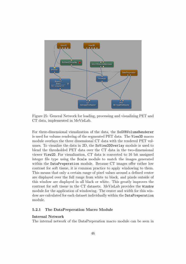
Figure 25: General Network for loading, processing and visualizing PET andCT data, implemented in MeVisLab.

For three-dimensional visualization of the data, the SoGVRVolumeRenderer

is used for volume rendering of the segmented PET data. The View3D macromodule overlays the three dimensional CT data with the rendered PET vol-umes. To visualize the data in 2D, the SoView2DOverlay module is used toblend the thresholded PET data over the CT data in the two-dimensionalviewer View2D. For visualization, CT data is converted to 16 bit unsignedinteger file type using the Scale module to match the images generatedwithin the DataPreperation module. Because CT images offer rather lowcontrast for soft tissue, it is common practice to apply windowing to them.This means that only a certain range of pixel values around a defined centerare displayed over the full range from white to black, and pixels outside ofthis window are displayed in all black or white. This greatly improves thecontrast for soft tissue in the CT datasets. MeVisLab provides the Window

module for the application of windowing. The center and width for this win-dow are calculated for each dataset individually within the DataPreperationmodule.

5.2.1 The DataPreperation Macro Module

Internal NetworkThe internal network of the DataPreperation macro module can be seen in

46

Figure 26: The internal network of the DataPreperation macro module.

figure 26. Generally, the network consists of two groups, one for CT and onefor PET image processing. In this section, the MeVisLab Image ProcessingLibrary (ML) Modules used and their purpose are explained.

• PET image processing:First, general information about the input image is extracted via theInfoPET module. This module provides information like image size,image type, maximal and minimal pixel value, etc. The Reformat

module reformats the PET dataset to the local coordinate system ofthe CT dataset using trilinear interpolation. This step is necessarybecause the PET and CT datasets do not have the same dimensions.The reformated image is then fed into the SubImagePET module. Thismodule allows the extraction of subregions from input images. Byiterating over the z-coordinate of a dataset and leaving the other pa-rameters unchanged, individual transversal slices can be selected andmanipulated. Next, the extracted PET slices are segmented by the ap-

47

plication of the Threshold module. A fixed threshold is calculated foreach dataset within the Python script. Every pixel above the thresholdis considered foreground, all other pixels are labelled as background.The output of this module is a binary image of the urinary blad-der. Data augmentation of the binary masks is performed using theAffineTransformation2DPET module. This module enables the ap-plication of several affine transformations in 2D. Translation, rotation,shearing and scaling can be entered, however, for this macro module,only rotation and scaling are enabled. Before saving the image, it isconverted to 8 bit unsigned integer and scaled to a range between 0and 255 using the ScalePET module. At last, the produced slices aresaved in TIFF format using the ImageSavePET module.

• CT image processing:Again, image information is obtained using the InfoCT module. Transv-ersal slices are extracted from the three-dimensional image data usingthe SubImageCT module. The CT images are converted and scaled to 16bit unsigned integer right away, because the AffineTransformation2Dmodule requires a datatype of 16 bit unsigned integer or lesser towork. In the AffineTransformation2DCT, the same transformationsas with the PET masks are applied to the CT slices. Additionally,the AddNoise module enables the addition of noise from various dis-tributions to the input image. In this project, uniformly distributed,zero-mean Gaussian and Salt and Pepper noise can be chosen. Even-tually, windowing is applied to the CT images to improve contrast forthe urinary bladder. Then again, the slices are saved as TIFF usingthe ImageSaveCT module.

MDL Script and PanelThe MDL Script DataPreperation.script consists of three main sections:

• The interface section defines the inputs (CT and PET image data)and outputs (no outputs are used for this module) of data connections.Furthermore, the parameters fields of the implemented macro moduleare declared here. The fields declared in the interface section can eitherbe independent script fields or they can be defined as aliases for internalfields of the internal network.

• The commands section defines the scripting file containing the func-tions to be executed upon the activation of certain fields. Also, thecommands for calling these functions are defined.

48

• The window section can be used to create a panel for the macro module,as seen in figure 27.

Figure 27: Panel of the DataPreperation macro module.

The DataPreperation module’s panel is shown in figure 27. It is used to setthe desired parameters and to monitor the progress of the file export. In theexport section of the panel, the user can enter or browse to the desired exportpaths to which the created images and labels will be saved. Furthermore, thefile name can be specified. It is also possible to choose between exporting allslices of the dataset or to only select certain slices.

The data augmentation section of the panel is for choosing the desired dataaugmentation steps and parameters. For rotation, the user can specify themaximal angle (in degrees) to which the images will be rotated. Furthermore,the number of rotations performed on each slice can be entered. The algo-rithm will then produce images that are rotated to equally distributed angles

49

between the negative and positive maximal rotation angle. When choosingscaling, the user can enter the desired maximal scale factor as well as thenumber of scaling steps performed in x- and y-direction. The algorithm willcalculate scale factors in a range defined by the maximal scale factor aroundone and will apply these scalings to the input images. If noise should beapplied to the input images, the number of slices generated can be speci-fied. Other parameters depend on the noise type. For uniform noise, themaximal noise amplitude can be entered. For zero-mean Gaussian noise, onemust define the maximal standard deviation and for salt and pepper noise,the maximal noise density is used as an input. An overview over all inputparameters, their default values and their minimal and maximal values isshown in table 1. Minimal, maximal and default values were chosen such tolimit the user to parameters that produce meaningful outputs.

By pressing the Calculate button, the number of images and labels createdwith the given parameters and for the specified slices are pre-calculated. Thisallows an easy overview over the amount of data obtained. Once all the pa-rameters are entered and the user is satisfied with the number of created data,the algorithm can be started by pressing the Export button. Progress of thedata export can be monitored via the progress bar at the bottom of the panel.

Table 1: Parameters for data augmentation. This table shows all parametersspecifiable by the user, as well as their default, minimal and maximal values.

Augmentation Type Parameter Default Minimum Maximum

RotationMaximal Rotation Angle 20 0 180Number of Rotations per Slice 3 1 9

Scaling

Maximal Scale Factor 0.1 0.05 0.15Number of Scalings in x-Direction 3 0 5Number of Scalings in y-Direction 3 0 5

Noise

Number of Noisy Slices 2 1 6

Uniform Maximal Amplitude 1500 500 2500zero-mean Gaussian Maximal Standard Deviation 500 100 1000Salt and Pepper Maximal Density 0.2 0.05 0.5

50

Python ScriptWithin the Python script, interactions between module fields, inputs, panelfields and outputs can be defined. This section gives an overview of the mostimportant functions implemented in the DataPreperation.py file.

When pressing the Export button on the panel, the function that is called isthe setThreshold() function. This function calculates the threshold T forsegmenting PET data and passes it to the Treshold module. The thresholdis defined as a fixed percentage, in this case 20%, of the maximal SUV withinthe dataset:

T = SUVmax · 0.2 (20)

The next function to be executed is the setWindow() function, which calcu-lates a suitable window center c for contrast enhanced visualization of softtissue in the CT data. For this, the following formula was derived:

c =65535

|Imin|+ Imax· 2800 (21)

where Imin and Imax are the minimal and maximal intensity value of the inputimage, respectively. As already mentioned, a CT contains Hounsfield valuesbetween -1024 HU and 3071 HU and the window center for soft tissue usuallylies around 0 HU. Our input images, however, have variable intensity rangesaround -3000 to +3000 and are already scaled to 16 bit unsigned integer,ranging between 0 and 65535. Therefore, these conversions have to be made.The factor 2800 was determined empirically to obtain optimal contrast forthe urinary bladder.

Next, the functions exportCT(field) and exportPET(field) are called.These functions check whether the export path specified by the user isvalid and then iterates over the slices to export, calling the main functionaugmentAndSafe for each slice. Furthermore, the progress bar is updated inthis function. The augmentAndSafe(...) performs the augmentation stepsspecified by the user and safes the generated data to the export directory. Theparameter name defines, whether PET or CT images are processed. Rotationangles, scaling factors and noise levels are determined using the respectivefunctions. Then, the algorithm loops over all these values and passes themto the corresponding fields in the AffineTransformation2D and Addnoise

modules. The file name is assembled by concatenating the input parame-ters and the transformation parameters, then the images or labels are saved.

51

The angles to which the input image should be rotated are calculated in thegetRotationAngles() function. If rotation is disabled, the rotation angleswill be set to zero. The function getScales returns all scaling factors towhich an image will be transformed. It returns scaling factors of one, if scal-ing is disabled. In the function getNoiseLevels, noise type and noise levelsare determined. For uniformly distributed noise, a range of noise amplitudesadded to the input image is returned. In case of gaussian noise, a range ofstandard deviations is calculated. For salt and pepper noise, a variation ofdifferent densities is returned. If the adding of noise is disabled, noise typeis set to none and all parameters are set to zero.

The function switchNoiseType() enables the input of different noise param-eters in the module panel, depending on which noise type was selected. Ifthe user activates the Calculate button in the panel, the function calcSlice

Number() is called to display the number of total slices generated from bothPET and CT data.

5.3 Image Segmentation using Deep Neural Networks

Algorithms for image segmentation using deep neural networks were imple-mented using TensorFlow 1.3 under Python 3.5. The code is divided up intoseveral files:

• tf records.py: Contains functions for creating and reading from theTensorFlow recommended file format TFRecords. Those functions areused to transform image data into a file format that is easy and fast toprocess in TensorFlow.

• make tfrecords dataset.py: This script can be used to put togethera TFRecords dataset from a directory of image files.

• networks.py: Includes the model definitions for the implemented im-age segmentation networks. These functions can be run in training ortesting mode.

• upsampling.py: Contains tools for creating bilinear upsampling fil-ters used for upsampling the predictions made by the networks usingtransposed convolution.

• FCN training.py and ResNet training.py: These scripts are used fortraining the deep neural network models defined in networks.py.

52

• FCN testing.py and ResNet testing.py: These scripts can be usedfor testing the previously trained deep neural networks.

• metrics.py: Provides metrics for evaluating the segmentation resultsby calculating similarity measures between network prediction and groundtruth.

5.3.1 Working with TFRecords files

There are two main ways of providing a TensorFlow program for training adeep neural network with data:

1. Feeding: The computation graph is constructed using placeholders,then data is loaded using python code and fed into the graph duringthe session.

2. Reading from files: The user provides a list of file names from which afile queue is created. The data is then read and decoded from this filequeue, during which batching and shuffling can be performed.

Since loading image data is a time-consuming operation, data is provided inthis project via reading from files. The standard, recommended TensorFlowformat for this is a TFRecords file. A TFRecords file represents a sequenceof binary strings, which enables the user to store images and ground truthannotations in a single binary file which is efficient to read. This way, theTFRecords file has to be created only once, and can then be used during ex-perimenting with and fine tuning the network without having to open imagedata individually each time.

Tools for writing and reading TFRecords files are found in the file tf records

.py. Writing image and label data into a TFRecords file is performed withthe function write to tfrecords(image path, label path, tfrecords

filename, height, width). The first step is to gather the filenames ofeach image specified in image path and label path. Those images are thenopened, resized to a resolution specifiable by the height and width param-eters, and converted to string. An Example called protocol buffer is puttogether from the data one wishes to store. Properties of the data set, likeimages, labels and image size, are stored within the protocol buffer as proto-cols called Features. Features have one of three base types: bytes, float orint64. The example buffer is then serialized and written to a TFRecords filespecified by tfrecords filename.

53

To read image data from the previously created TFRecords file, the functionread and decode(tfrecords filename) was created. The name of a suit-able TFRecords file is passed to this function in tfrecords filename fromwhich records are read and decoded by taking the serialized examples andmapping the features back to tensor values. At first, image and label datais parsed in string format, then this raw data is decoded to unsigned integer8. Since image dimensions are lost when converting image data to string,images and labels have to be reshaped to their original dimensions. For this,image height and width are parsed from the TFRecords file as integer values.

5.3.2 Creating TFRecords files for Training and Testing

The file make tfrecords dataset.py contains a script for writing image datato TFRecords using the function described above. Paths to image and cor-responding label data must be provided. Furthermore, the user can specifythe target resolution of images and labels. This script was used to produceseveral TFRecords files used for further training and testing. From each rawimage dataset TFRecords files containing images and labels downsampledby a factor of two to a resolution of 256×256 were created. Furthermore,two TFRecords files were generated from the unaugmented and transformedtraining data. Due to the unsatisfactory performance of training data withadditional noise in the case of downsampled images and the long trainingtimes, we refrained from training our networks with fully augmented imagesat their full resolution.

Testing data was also converted to TFRecords files with one file containingdownsampled images of resolution 256×256 and one file with original imageresolution. Table 2 provides an overview over the created files. It shows thefilenames of the TFRecords files, the augmentations applied, the resolutionas well as the total number of labelled images within the dataset.

5.3.3 Segmentation Networks using TF-Slim and pre-trained Clas-sification Networks

Neural networks for complex tasks like image segmentation need to be largeand deep, resulting in many thousands of parameters. This means that train-ing such networks requires huge datasets and a lot of computational power,and the training process might still require days or even weeks to complete.Therefore, pre-trained models were used for the segmentation task at hand.The TF-Slim API contains a set of standard model definitions implemented

54

Table 2: Created TFRecords files for training and testing.

File Name Augmentations Image Resolutions Number of Images

Training NoAug 256.tfrecords none 256x256 630

Training NoAug 512.tfrecords none 512x512 630

Training TransAug 256.tfrecords rotation, scaling 256x256 17010

Training TransAug 512.tfrecords rotation, scaling 512x512 17010

Training FullAug 256.tfrecords rotation, scaling, noise 256x256 34020

Testing 256.tfrecords none 256x256 215

Testing 512.tfrecords none 512x512 215

with TF-Slim as well as checkpoints for pre-trained parameters. An overviewof the implemented models, corresponding code and links to the model check-points can be found at [59]. The models were trained on the ILSVRC-2012dataset for image classification. The TF-slim model library contains imple-mentations of VGG 16 and ResNet V2, which are adapted for segmentationtasks, as explained in section 4.2.

The model definitions of the implemented segmentation networks are foundin the file networks.py. The implementation of these models is based onthe implementation found in [60]. The first network definition, FCN(...)

uses a pre-trained version VGG 16, which is already implemented in a fullyconvolutional way in the TF-slim model library, which means that the lastthree fully connected layers are also implemented as convolutional layers. Bycalling the vgg.vgg 16(...) function using ’SAME’ padding, a map of un-scaled log probabilities of the classes (logits), downsampled by a factor of 32,is returned. Furthermore, a dictionary called end points is obtained, whichcontains the logits of each network layer. These coarse feature maps are thenupsampled using bilinear interpolation and skip connections, resulting in aFCN 8s architecture as described by Long et al. in [38]. In the first step,logits of the last layer are upsampled by factor two. Features produced bythe pool4 layer of the VGG 16 classification network are extracted from theendpoints and combined with the upsampled final logits. The combination isonce again upsampled by a factor of two, and then combined with the featuresobtained from the pool3 layer. As a last step, this combination is upsampledby a factor of eight, to produce an output of the same size as the originalinput to the classification network. This output represents the final unscaledlog probabilities of the FCN 8s model and is returned by the function. Notethat while upsampling filters could be defined as a learnable variable, theyare kept fixed in this model, since Long et al. stated in their paper that

55

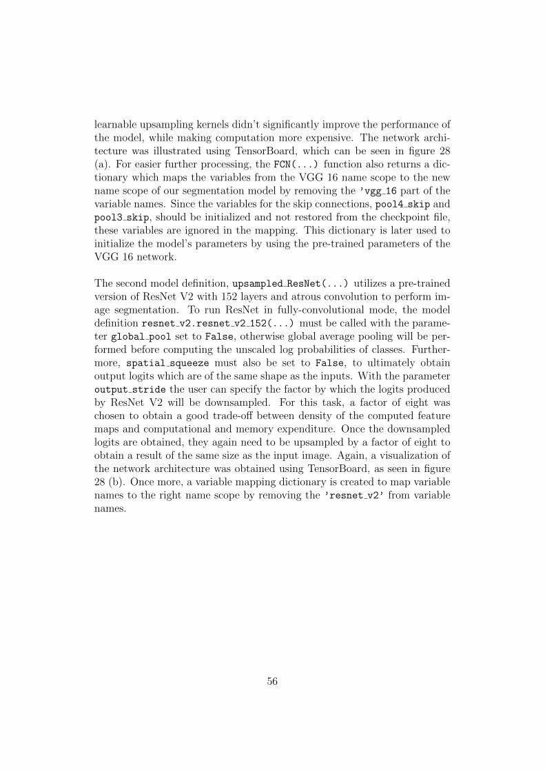
learnable upsampling kernels didn’t significantly improve the performance ofthe model, while making computation more expensive. The network archi-tecture was illustrated using TensorBoard, which can be seen in figure 28(a). For easier further processing, the FCN(...) function also returns a dic-tionary which maps the variables from the VGG 16 name scope to the newname scope of our segmentation model by removing the ’vgg 16 part of thevariable names. Since the variables for the skip connections, pool4 skip andpool3 skip, should be initialized and not restored from the checkpoint file,these variables are ignored in the mapping. This dictionary is later used toinitialize the model’s parameters by using the pre-trained parameters of theVGG 16 network.

The second model definition, upsampled ResNet(...) utilizes a pre-trainedversion of ResNet V2 with 152 layers and atrous convolution to perform im-age segmentation. To run ResNet in fully-convolutional mode, the modeldefinition resnet v2.resnet v2 152(...) must be called with the parame-ter global pool set to False, otherwise global average pooling will be per-formed before computing the unscaled log probabilities of classes. Further-more, spatial squeeze must also be set to False, to ultimately obtainoutput logits which are of the same shape as the inputs. With the parameteroutput stride the user can specify the factor by which the logits producedby ResNet V2 will be downsampled. For this task, a factor of eight waschosen to obtain a good trade-off between density of the computed featuremaps and computational and memory expenditure. Once the downsampledlogits are obtained, they again need to be upsampled by a factor of eight toobtain a result of the same size as the input image. Again, a visualization ofthe network architecture was obtained using TensorBoard, as seen in figure28 (b). Once more, a variable mapping dictionary is created to map variablenames to the right name scope by removing the ’resnet v2’ from variablenames.

56

(a) FCN architecture (b) upsampled ResNet architecture

Figure 28: Network Graphs for FCN and upsampled ResNet visualized withTensorBoard. Figure (a) shows the implemented FCN architecture, which isbased on a pre-trained VGG 16 network and upsampling with skip connec-tions. Figure (b) shows our upsampled ResNet architecture, which is basedon a pre-trained ResNet V2 152 network. The layers of this network arecondensed within 4 building blocks.

57

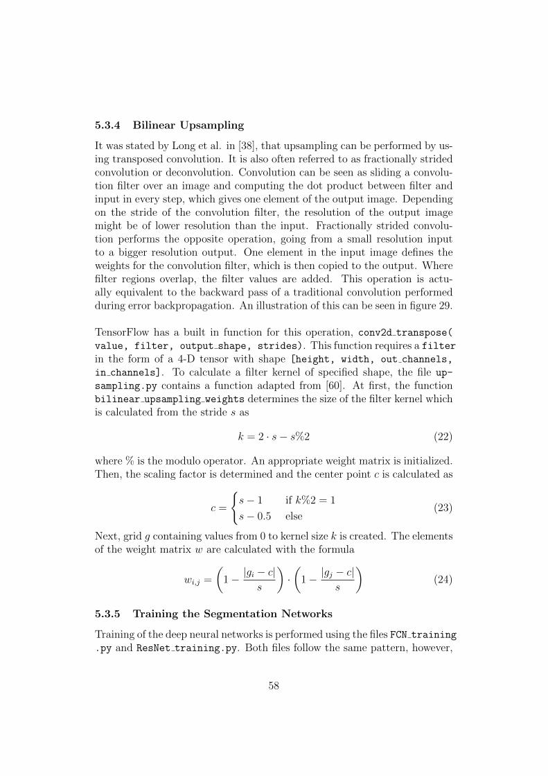
5.3.4 Bilinear Upsampling

It was stated by Long et al. in [38], that upsampling can be performed by us-ing transposed convolution. It is also often referred to as fractionally stridedconvolution or deconvolution. Convolution can be seen as sliding a convolu-tion filter over an image and computing the dot product between filter andinput in every step, which gives one element of the output image. Dependingon the stride of the convolution filter, the resolution of the output imagemight be of lower resolution than the input. Fractionally strided convolu-tion performs the opposite operation, going from a small resolution inputto a bigger resolution output. One element in the input image defines theweights for the convolution filter, which is then copied to the output. Wherefilter regions overlap, the filter values are added. This operation is actu-ally equivalent to the backward pass of a traditional convolution performedduring error backpropagation. An illustration of this can be seen in figure 29.

TensorFlow has a built in function for this operation, conv2d transpose(

value, filter, output shape, strides). This function requires a filterin the form of a 4-D tensor with shape [height, width, out channels,

in channels]. To calculate a filter kernel of specified shape, the file up-

sampling.py contains a function adapted from [60]. At first, the functionbilinear upsampling weights determines the size of the filter kernel whichis calculated from the stride s as

k = 2 · s− s%2 (22)

where % is the modulo operator. An appropriate weight matrix is initialized.Then, the scaling factor is determined and the center point c is calculated as

c =

{s− 1 if k%2 = 1

s− 0.5 else(23)

Next, grid g containing values from 0 to kernel size k is created. The elementsof the weight matrix w are calculated with the formula

wi,j =

(1− |gi − c|

s

)·(

1− |gj − c|s

)(24)

5.3.5 Training the Segmentation Networks

Training of the deep neural networks is performed using the files FCN training

.py and ResNet training.py. Both files follow the same pattern, however,

58

Figure 29: Comparison between normal convolution and transposed convo-lution. Both operations use a 3×3 kernel and a stride of two. Traditionalconvolution determines the output value as the dot product between filterand input, by moving the filter kernel for two pixels in every step, the inputis downsampled by factor two. For transposed convolution, the input valuedetermines the filter values that will be written to the output. Where fil-ters overlap, the values are summed up. The stride defines the movement ofthe filter kernel in the output image, and therefore influences the factor ofupsampling.

since networks are trained from different checkpoint files, there are some dif-ferences between training a fully convolutional network and an upsampledResNet network. While the FCN architecture requires a VGG 16 checkpointto work, a ResNet V2 152 checkpoint is needed for the upsampled ResNetarchitecture. Segmentation is performed into two classes, background andforeground (urinary bladder), so the number of classes is chosen accordingly.Batch size is chosen as 1 as it was in the original architectures. A largerbatch size would result in tensor sizes exceeding GPU memory. A batch sizeof 1 means that each image will be processed individually and no batch nor-malization is performed. Then, images and labels are loaded from a specifiedTFRecords training data file.

Next, random batching of the obtained image data is performed. The func-

59

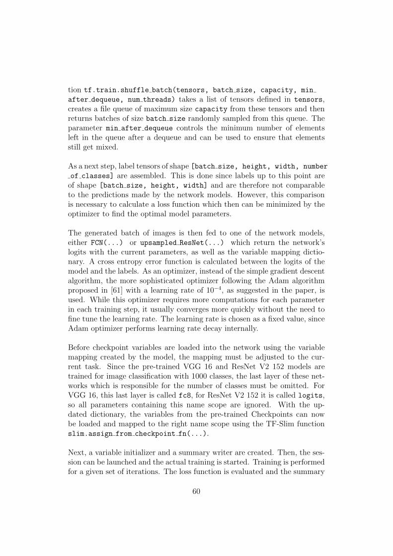
tion tf.train.shuffle batch(tensors, batch size, capacity, min

after dequeue, num threads) takes a list of tensors defined in tensors,creates a file queue of maximum size capacity from these tensors and thenreturns batches of size batch size randomly sampled from this queue. Theparameter min after dequeue controls the minimum number of elementsleft in the queue after a dequeue and can be used to ensure that elementsstill get mixed.

As a next step, label tensors of shape [batch size, height, width, number

of classes] are assembled. This is done since labels up to this point areof shape [batch size, height, width] and are therefore not comparableto the predictions made by the network models. However, this comparisonis necessary to calculate a loss function which then can be minimized by theoptimizer to find the optimal model parameters.

The generated batch of images is then fed to one of the network models,either FCN(...) or upsampled ResNet(...) which return the network’slogits with the current parameters, as well as the variable mapping dictio-nary. A cross entropy error function is calculated between the logits of themodel and the labels. As an optimizer, instead of the simple gradient descentalgorithm, the more sophisticated optimizer following the Adam algorithmproposed in [61] with a learning rate of 10−4, as suggested in the paper, isused. While this optimizer requires more computations for each parameterin each training step, it usually converges more quickly without the need tofine tune the learning rate. The learning rate is chosen as a fixed value, sinceAdam optimizer performs learning rate decay internally.

Before checkpoint variables are loaded into the network using the variablemapping created by the model, the mapping must be adjusted to the cur-rent task. Since the pre-trained VGG 16 and ResNet V2 152 models aretrained for image classification with 1000 classes, the last layer of these net-works which is responsible for the number of classes must be omitted. ForVGG 16, this last layer is called fc8, for ResNet V2 152 it is called logits,so all parameters containing this name scope are ignored. With the up-dated dictionary, the variables from the pre-trained Checkpoints can nowbe loaded and mapped to the right name scope using the TF-Slim functionslim.assign from checkpoint fn(...).

Next, a variable initializer and a summary writer are created. Then, the ses-sion can be launched and the actual training is started. Training is performedfor a given set of iterations. The loss function is evaluated and the summary

60

is updated in each step. Every 100th iteration, the current loss is printedto allow easy monitoring of the training process. Furthermore, the currentmodel parameters are saved to the checkpoints directory every 1000th step,as well as after training has finished.

5.3.6 Testing the Segmentation Networks

For testing the neural network models, the files FCN testing.py and ResNet

testing.py are provided. Similar to the scripts for training, both files havethe same structure and only differ in the used model definition and check-point files. After defining the paths to checkpoint files and the testing data,once again, image data is read and decoded from the specified TFRecordsfile. This time, random batching is not performed. However, since the neuralnetwork model definitions require a tensor of shape [batch size, height,

width, depth] to work, an additional dimension has to be added to the im-age and label tensors. Afterwards, inference is performed to obtain unscaledlog probabilities of classes. To obtain a binary prediction, meaning a tensorcontaining zeroes and ones, from these logits, tf.argmax is applied. For cal-culating normalized probabilities of classes, the softmax function tf.softmax

is used. Next, the similarity metrics true positive rate, true negative rate anddice coefficient are calculated. Those metrics will be discussed in more detailin the next section. Before starting the session, variables and checkpointsaver are initialized.

Within the session, parameters trained in the previous step are loaded intothe model. Vectors for calculating the evaluation metrics are initialized andthe number of iterations performed, corresponding to the size of the testingdataset, is specified. The current image, label, prediction, scaled probabil-ities as well as the Dice coefficient are evaluated at every testing iteration.The Hausdorff distance similarity metric is calculated within the session us-ing numpy arrays instead of Tensors, which proved to be more efficient sincethe numpy library already contains many operations needed for calculation.Note that Hausdorff distance is only calculated for samples where both pre-diction and label are not empty, e.g. containing at least one pixel belongingto the foreground. Metric values are stored in their corresponding vectors.Images, corresponding labels and predictions are saved in jpeg file formatto a specifiable directory. Furthermore, the option to display a sample ofinput images, their corresponding label and the prediction made by the seg-mentation network is implemented here. After the testing loop is finished,the mean of true positive rate (TPR), true negative rate (TNR), Dice co-efficient (DSC) and Hausdorff distance (HD) are calculated. Furthermore,

61

histograms of TPR, TNR, DSC and HD are created. Histograms of theseevaluation metrics are useful for evaluating per-image scores of the dataset.Per-image scores are important because measures averaged over the wholetesting dataset are not suitable to distinguish between algorithms that per-form mediocre on all images and algorithms that perform very well on someimages, but very bad on others [62].

5.3.7 Evaluation Metrics

To evaluate the results achieved with the proposed neural networks, sev-eral metrics that are commonly applied for measuring similarity between theground truth and the segmentation result when working with medical imagedata are calculated. True Positive Rate, True Negative Rate and Dice co-efficient are metrics commonly found in literature. However, these metricsmight be a poor measure for images with a lot of background and small ob-ject segments. Therefore, the Hausdorff distance is additionally measured. Itis also a useful estimate when the boundary delineation of the segmentationis of special interest, as it is the case in this thesis. However, it should benoted that Hausdorff distance is very sensitive to outliers [63]. Functions forcalculating evaluation metrics are found in the file metrics.py

True Positive Rate and True Negative RateThe true positive rate (TPR), commonly referred to as sensitivity, measuresthe amount of positive pixels (foreground pixels) in the ground truth that arealso identified as positives by the segmentation algorithm. The true negativerate (TNR), also called specificity, on the other hand, measures the portionof negative pixels (background pixels) in the ground truth segmentation thatare correctly identified as such by the algorithm. The measures are definedas

TPR =TP

TP + FN(25)

and

TNR =TN

TN + FP(26)

where

• TP are the true positives, meaning pixels which are correctly classifiedto the foreground

• FN are false negatives, pixels that are incorrectly classified to the back-ground

62

• TN are true negatives, pixels which are correctly assigned to back-ground

• FP are false positives, meaning pixels that are incorrectly identified asforeground [64].

Calculation of TPR and TNR can be performed with the functions tpr(label,prediction) and tnr(label, prediction), respectively.

Dice CoefficientThe Dice coefficient [65], also called Sorensen-Dice coefficient (DSC), is themost used metric for validating medical image segmentation. It is an overlapbased metric. For a ground truth segmentation Sg and a predicted segmen-tation Sp, the DICE can be calculated as

DSC =2|Sg ∩ Sp||Sg|+ |Sp|

(27)

where |Sg ∩ Sp| is the intersection between ground truth segmentation andpredicted segmentation. This intersection corresponds to the true positivesTP . |Sg| and |Sp| denote the total amount of pixels classified to foregroundin the ground truth and the prediction, respectively. The DSC takes valuesbetween 0 and 1, where 1 equals a perfect match. DSC calculation is imple-mented in the function DSC coeff(label, prediction).

Hausdorff DistanceThe Hausdorff distance (HD) is a spatial distance based similarity measure,which means that the spatial position of pixels are taken into consideration.The Hausdorff distance between two point sets A and B is defined as

HD(A,B) = max(h(A,B), h(B,A)) (28)

where h(A,B) is the directed Hausdorff distance. It describes the maximaldistance of point set A to the closest point in point set B. It’s mathematicaldefinition is

h(A,B) = maxa∈A

minb∈B‖a− b‖ (29)

where a and b are points of point set A and B respectively and ‖...‖ is a norm,in example `2 norm to calculate Euclidian distance between the two points.A graphical representation of the Hausdorff distance and directed Hausdorffdistance can be seen in figure 30. The Euclidian distance can be calculatedby

‖a− b‖2 =

√∑i

(ai − bi)2 (30)

63

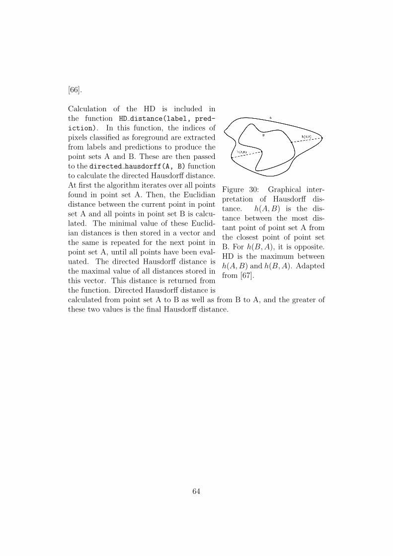
[66].

Figure 30: Graphical inter-pretation of Hausdorff dis-tance. h(A,B) is the dis-tance between the most dis-tant point of point set A fromthe closest point of point setB. For h(B,A), it is opposite.HD is the maximum betweenh(A,B) and h(B,A). Adaptedfrom [67].

Calculation of the HD is included inthe function HD distance(label, pred-

iction). In this function, the indices ofpixels classified as foreground are extractedfrom labels and predictions to produce thepoint sets A and B. These are then passedto the directed hausdorff(A, B) functionto calculate the directed Hausdorff distance.At first the algorithm iterates over all pointsfound in point set A. Then, the Euclidiandistance between the current point in pointset A and all points in point set B is calcu-lated. The minimal value of these Euclid-ian distances is then stored in a vector andthe same is repeated for the next point inpoint set A, until all points have been eval-uated. The directed Hausdorff distance isthe maximal value of all distances stored inthis vector. This distance is returned fromthe function. Directed Hausdorff distance iscalculated from point set A to B as well as from B to A, and the greater ofthese two values is the final Hausdorff distance.

64

6 Results and Evaluation

In this chapter, we present the results of our experiments. It starts withsome examples taken from the training datasets to document the agreementbetween image data and generated labels, as well as the effects of data aug-mentation. In the second section 6.2, training and testing times using thetwo different architectures and different training datasets are evaluated. Seg-mentation results obtained from the various models described in this thesisare presented in section 6.3. Quantitative results are given in the form ofvarious segmentation evaluation scores as well as their histograms to allowper-image evaluation. Furthermore, examples of qualitative segmentationresults are shown.

6.1 Generation of Training and Testing Data

To illustrate the agreement between the ground truth labels obtained fromthresholding the PET data and corresponding CT images, overlays betweenCT images and generated labels were produced. Some examples of theseoverlays can be seen in figure 31.

(a) (b) (c)

(d) (e) (f)

Figure 31: Examples of overlays between CT data and generated groundtruth labels. The underlying CT images are shown in greyscale, while theground truth labels obtained from PET segmentation are added in red.

65

By applying data augmentation with the default parameters specified in ta-ble 1 to the original 630 training images, a total amount of 34,020 augmentedimages and labels were obtained. This equals a magnification factor of theoriginal dataset by 54. A magnification factor of 27 was achieved by thetransformation, specifically the combination of rotations and scaling of theinput images. The amount of transformed data was then doubled by theaddition of zero-mean Gaussian noise on each image slice. The remainingnoise types included in the DataPreperation MeVisLab macro module havenot yet been explored. By fully exploiting the maximal parameters definedin table 1, a magnification factor of up to 1350 could be achieved, whichwould result in a total of 850,500 augmented image slices. However, sincesuch large amounts of data are hard to handle with the available resources,such a large dataset was not created. A sample taken from the augmentedtraining data is shown in figure 32.

(a) Original (b) Rotated andscaled

(c) Added noise

Figure 32: Example for an augmented dataset. Image (a) shows the originalCT image and ground truth label without augmentations. Image (b) showsthe dataset after applying a rotation of 20◦ and scaling to a scale factorof 0.9 in x-direction and 1.1 in y-direction to both the CT image and thebinary mask. In image (c), zero-mean Gaussian noise with a standard devi-ation of 500 was added to the transformed image. The binary mask remainsunchanged by the addition of noise.

66

6.2 Training and Testing

Training was performed for 34,020 iterations (corresponding to the size of thelargest training data set) on a server equipped with a NVIDIA Tesla K20Xmwith 5 GB memory size. Testing was executed using a NVIDIA GeForceGTX 960 with 2 GB of memory.

On average, FCN models took 21 hours to train with images with a resolu-tion of 256×256, while upsampled ResNet architectures took an average of39 hours of training time with the same datasets. For images at their originalresolution, training an FCN architecture required 71 hours on average, whilefor a ResNet architecture, 115 hours were needed. Table 3 gives a comparisonover the time required to train our network models with the stated trainingdata. Furthermore, the average time needed to perform inference, which isthe average time needed to calculate a prediction for a single input imagefrom the training dataset, is stated.

Table 3: Comparison of training and inference times. Training time is givenin hours needed to complete the training process, inference time is averagedover all testing samples and given in milliseconds.

Network Model Image Resolution Training DataTraining Time av. inference time

(hours) (ms)

FCN

256×256

no augmentation 24 9.7transformed images 14 9.9

fully augmented images 25 9.8

512×512no augmentation 56 18.4

transformed images 86 17.7

upsampled ResNet

256×256

no augmentation 62 108.2transformed images 27 108.6

fully augmented images 28 108.0

512×512no augmentation 99 219.4

transformed images 130 222.6

A visualization of the development of cross-entropy loss during training ob-tained from TensorBoard can be seen in appendix B, figure 36.

67

6.3 Image Segmentation Results

Table 4 shows the results of segmentation evaluation for models trained withdifferent training datasets at a resolution of 256×256. Table 5 presents thesame metrics for segmentation results obtained from models with images attheir original resolution. True positive rate, true negative rate, Dice coeffi-cient, each in percent, and Hausdorff distance, in pixels, averaged over all215 training datasets are listed.

Table 4: Segmentation evaluation results for images rescaled to 256×256.This Table compares evaluation metrics for FCN and upsampled ResNetarchitectures trained using unaugmented training data, transformed trainingdata (rotation, scaling) and fully augmented training data (transformationsand zero-mean Gaussian noise).

Network Model Training Datamean TPR mean TNR mean DSC mean HD

(%) (%) (%) (pixel)

FCN

no augmentation 82.7 99.9 77.6 6.9transformed images 85.0 99.9 80.4 6.1fully augmented images 79.2 99.9 77.6 6.7

upsampled ResNet

no augmentation 80.7 99.9 73.5 7.9transformed images 82.5 99.9 76.9 6.3

fully augmented images 79.7 99.9 76.7 7.7

Table 5: Segmentation evaluation results for images of resolution 512×512.This Table compares evaluation metrics for FCN and upsampled ResNet ar-chitectures trained using unaugmented training data and transformed train-ing data (rotation, scaling).

Network Model Training Datamean TPR meanTNR mean DSC mean HD

(%) (%) (%) (pixel)

FCNno augmentation 80.9 99.9 77.6 13.3

transformed images 83.1 99.9 81.9 11.9

upsampled ResNetno augmentation 68.7 99.9 71.1 23.9

transformed images 86.5 99.8 67.1 16.9

To visualize per-image evaluation scores of our models, the Histograms infigure 33 of evaluation metrics (true positive rate, true negative rate, Dicecoefficient and Hausdorff distance) were plotted.

68

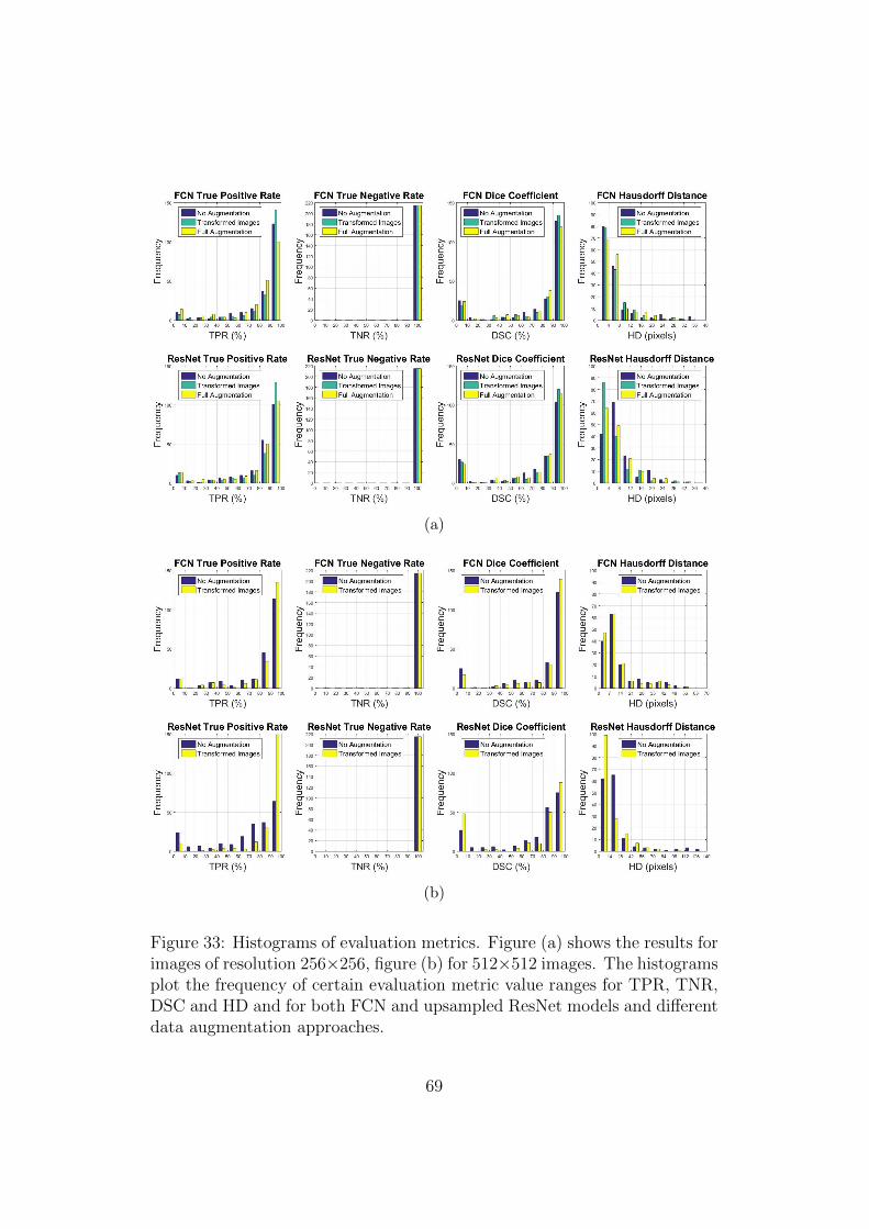
(a)

(b)

Figure 33: Histograms of evaluation metrics. Figure (a) shows the results forimages of resolution 256×256, figure (b) for 512×512 images. The histogramsplot the frequency of certain evaluation metric value ranges for TPR, TNR,DSC and HD and for both FCN and upsampled ResNet models and differentdata augmentation approaches.

69

Figures 34 and 35 show several representative examples of the obtained seg-mentation results for images downsampled to a resolution of 256×256 andimages at original resolution of 512×512, respectively. For better illustra-tion, original image data was overlaid with the contour of the ground truthin green as well as the prediction made by our deep networks in red. Originalimage, label and prediction data is shown in appendix C, figures 37 and 38.

Sample (a) Sample (b) Sample (c) Sample (d) Sample (e)

FCN trained

with

unaugmented

data

FCN trained

with

transformed

data

FCN trained

with fully

augmented data

ResNet trained

with

unaugmented

data

ResNet trained

with

transformed

data

ResNet trained

with fully

augmented data

Figure 34: Qualitative segmentation result overlays for images scaled to256×256. Ground truth labels are shown by the contours in green, the pre-dictions made by the deep learning models are overlaid in red.

70

Sample (a) Sample (b) Sample (c) Sample (d) Sample (e)

FCN trained

with

unaugmented

data

FCN trained

with

transformed

data

ResNet trained

with

unaugmented

data

ResNet trained

with

transformed

data

Figure 35: Qualitative segmentation result overlays for images with resolu-tion 512×512. Ground truth labels are shown by the contours in green, thepredictions made by the deep learning models are overlaid in red.

71

7 Discussion

Agreement between Image Data and Ground Truth

Concerning the evaluation of agreement between CT data and the groundtruth labels generated from PET data, it can be observed that agreement isgenerally good, but not perfect. Examples are shown in figure 31. However,accuracy differs from dataset to dataset and even within individual slices. Itcan be observed that accuracy is worse in images were the urinary bladderonly covers a small area surface of the image, like in image 31 (d) and (f).This is due to the nature of PET imaging, which has low spatial resolutionand therefore, object boundaries might appear blurred. This is especiallyproblematic when objects are small.

Figure 31 also shows some of the unique challenges one is confronted withwhen automatically segmenting the urinary bladder in CT images. It canbe noted that size and position of the urinary bladder is varying betweenpatients. In some image slices, for example in figure 31 (c), the shape of theurinary bladder highly differs from it’s conventional, round form. Further-more, low contrast between the bladder and surrounding soft tissue, as seenin figure 31 (b), poses a big difficulty. This especially occurs at the ambiguousbladder-prostate interface, as shown in figure 31 (e). It also becomes evidentthat not all CT data offers the same quality. In example, images 31 (c) and(f) show noticeable streak artefacts. Those artefacts are commonly found inCT scans and appear between dense objects like bone or metal due to beamhardening. Furthermore, since feature maps are significantly downsampledwithin our network architectures, images with a small area surface of theurinary bladder, as seen in figure 31 (f) might pose a problem, since smalldetails could be lost as a result of downsampling.

Influence of Data Augmentation on Segmentation Performance

Segmentation evaluation results in tables 4 and 5 show that the application ofdata augmentation in the form of scaling and rotation to the original datasetdoes improve segmentation performance significantly. For mean TPR andDSC an increase of 2.3% and 2.8%, respectively, was achieved with the FCNarchitecture and training and testing images with resolution of 256×256. Fordata with resolution 512×512 a similar increase of 2.1% mean TPR and 4.3%mean DSC was achieved. With the upsampled ResNet architecture the cor-responding enhancement was 1.8% and 3.5% with downsampled images or17.8% TPR and a decrease of 4% DSC with original image resolution. Av-erage Hausdorff distance was decreased by 0.8 pixels and 1.4 pixels in FCN

72

models, as well as 1.6 pixels and 7 pixels using upsampled ResNet for the256×256 and 512×512 datasets, respectively. The mean true negative rateexhibited very high values regardless of the used network model and shows nosignificant variations between different training data sets. Although trans-formation of training data did increase segmentation performance, it can benoted that segmentation results obtained from the network trained with theoriginal dataset consisting of only 630 images and labels are also quite satis-factory for models trained with downsampled image resolution. This showsthat when using pre-trained networks, one can achieve passable results withonly a small amount of training data.

From the evaluation scores achieved with models trained with fully aug-mented data in table 4, it can be seen that the addition of noise to thetransformed training dataset does not improve the performance of of our pro-posed networks. In fact, all metrics show a worse performance of networkstrained with artificially noisy training data compared to networks trainedwith only transformed training data. Using the FCN architecture, meanTPR even showed higher results when the network was only trained with630 un-augmented training sets, with a TPR of 82.7% compared to 79.2%achieved with the fully augmented training set. The same is true for the up-sampled ResNet architecture, although to a lesser extend, with an achievedTPR of 80.7% using un-augmented data compared to 79.7% using fully aug-mented data. One explanation for this could be that the applied Gaussiannoise is not meaningful in the presented context. Therefore, the networklearns spurious patterns that are not present in the training data. Anotherreason for the decrease in performance might be that the added noise is notstrong enough. This results in the model seeing very similar images repeat-edly, which might lead to overfitting. The model starts to fit too specific tothe training set and loses it’s ability to generalize to the new examples foundin the testing set. Since we didn’t obtain satisfactory results with the noisytraining data, network architectures were not trained with this data at it’soriginal resolution of 512×512.

Segmentation Results

The comparison of our FCN and upsampled ResNet architectures trainedwith differently augmented datasets in table 4 shows that in case of imagesrescaled to 256×256, best results can be achieved with the FCN architecturetrained with images that are augmented with scaling and rotation. This net-work resulted in the highest true positive rate (85.0%) and Dice coefficient(80.4%) as well as the lowest Hausdorff distance (6.1 pixels). The true nega-

73

tive rate at 99.9% is the same for all tested models. The very high specificityindicates that our models are very accurate when it comes to correctly la-belling background. However, this measure is highly dependent on segmentsize. Images with a lot of background, as it is the case in our examples,naturally show a higher TNR. Regardless of the used training data, the FCNarchitecture outperforms the upsampled ResNet architecture in all evalua-tion metrics. Moreover, the comparison of training and inference times intable 3 shows that our FCN architecture is significantly faster. On average,it took 21 hours to train our FCN models with images of resolution 256×256,while it took 39 hours to train the upsampled ResNet models with the samedatasets. When calculating a prediction from a single input image, our FCNmodels show an average inference time of 9.8 ms, which is over 10 times fasterthan the average inference time of the upsampled ResNet architectures withan average inference time of 108.3 ms.

Inspecting the evaluation results using images at their original resolution of512×512 in table 5, again, the FCN architecture generally performs betterin terms of our evaluation metrics. Especially Dice coefficient is notablyhigher at 81.9% for FCN than for ResNet at 67.1% for our best performingmodels. Also, the Hausdorff distance is shorter by 5 pixels, indicating thatour upsampled ResNet architecture produces more outliers. Only in termsof true positive rate, the ResNet architecture achieved better results with aTPR of 86.5 % compared to 83.1% for the FCN architecture. Again, trainingand inference times are also considerably lower for FCNs than for upsampledResNets.

Looking at per-image evaluation of our models illustrated by histograms infigure 33, it is evident that frequency distribution of our evaluation met-rics is similar for FCN and upsampled ResNet. It is still recognizable thatFCN performance is in general slightly better than upsampled ResNet perfor-mance. Looking at the True Positive Rate, it can be seen that most testingimages by far were segmented with a TPR between 90% and 100%. There isalso a significant amount of testing sets with a TPR between 80% and 90%,which can also be considered a good result. However, a not negligible num-ber of images resulted in a very low TPR between 0% and 10%. The sameis even more clear when looking at the Dice coefficient. While most testingimages resulted in a DSC of 80% or higher, up to more than 25 images fromour testing dataset were segmented with a DSC between 0% and 10%. Af-ter inspecting our qualitative segmentation results, it became apparent thatmost of these incorrectly segmented images are false positives. Our modelsfrequently produced a prediction for testing datasets in which the CT im-

74

age did not show a segment of the urinary bladder and correspondingly, theground truth label was empty. Additionally, a couple of false negatives wereproduced, primarily in image slices were the urinary bladder had a small areasurface plus the image possessed rather low soft tissue contrast. Looking atHausdorff distance distribution, it can be seen that most testing datasetsresulted in a HD of zero to four pixels. After that, frequency exponentiallydecreases. However, Hausdorff distance reaches very high values for up to 40pixels in some images which indicates that our models sometimes produceoutliers in the segmentation.

The qualitative segmentation results for images scaled to 256×256 shown infigure 34 illustrate that for input images with good soft tissue contrast, alarge, homogeneous area surface and a regular shape of the urinary blad-der, as seen in sample (a), all network models perform well. In sample (b),contrast between the urinary bladder and surrounding tissue is not ideal,moreover, the bladder itself includes varying grey values, meaning that thearea surface is not homogeneous. It is evident that while our FCN archi-tecture has no trouble in detecting the urinary bladder in these images, theupsampled ResNet architecture performs poorly. Apparently the upsampledResNet models are more sensitive against contrast and grey values. How-ever, it can be seen from sample (c), that the ResNet models are better inadapting to distinct shapes. Sample (d) is interesting because our generatedground truth annotation does not follow the very unusual shape of the blad-der very well in this example. While the ResNet models seem to fit betterto the ground truth label, the segmentation predicted by the FCN models,especially the network trained with transformed data, seems to correspondbetter to the actual outline of the bladder. Sample (e) shows, that despiteour initial concerns, the proposed models are able to identifying the urinarybladder when only a small portion of it is visible in a slice, as long as con-trast is good. In fact, the predictions made by our models in some cases evenfollow the outline of the urinary bladder better than our underlying groundtruth segmentation.

The same observations can be made when looking at the qualitative segmen-tation results for images of higher resolution in figure 35. For input imagesof high quality, both architectures perform well. FCN does better when seg-menting images with low contrast and inhomogeneous grey values as seenin sample (b), while ResNet adapts better to unusual shapes as in sample(c). Again, sample (d) allows for some very interesting observations. Here,our upsampled ResNet architecture does a very good job in detecting theurinary bladder, even recognising the small, detached portion of the bladder

75

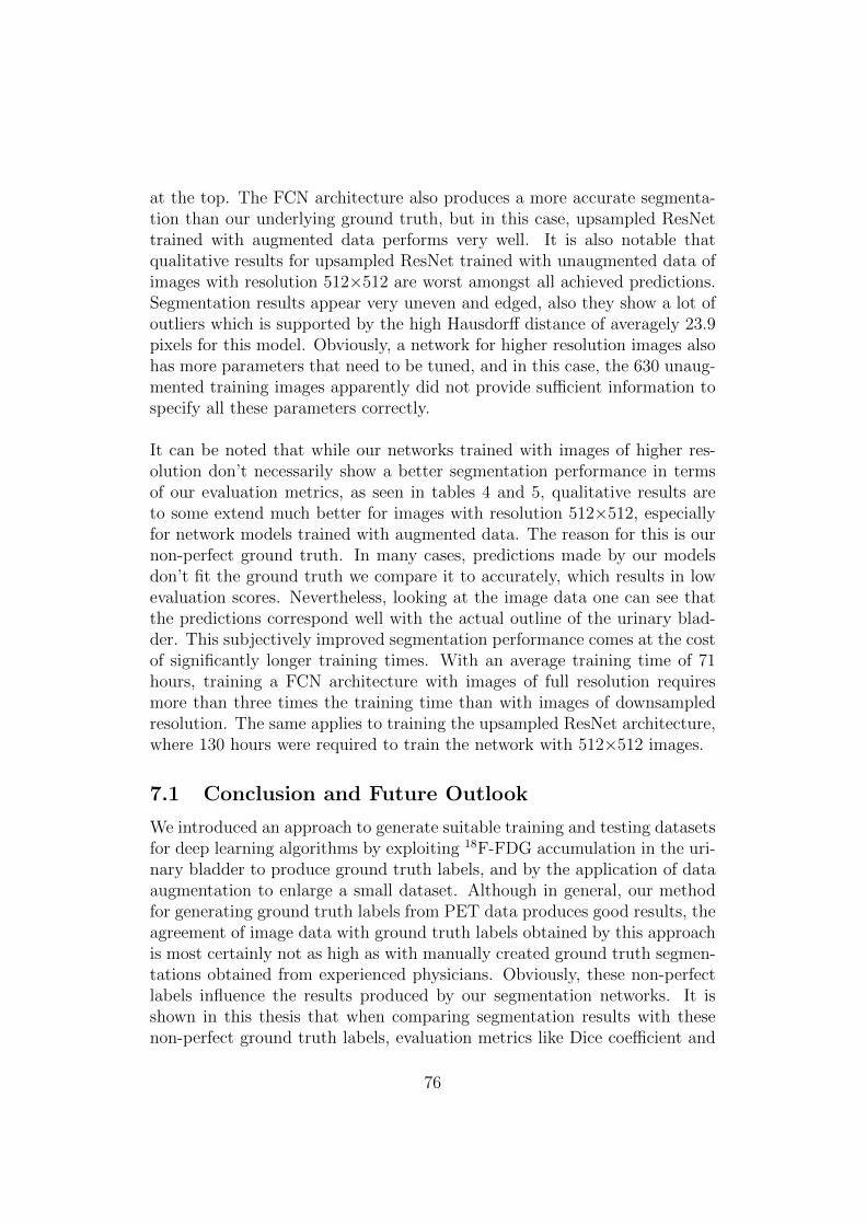
at the top. The FCN architecture also produces a more accurate segmenta-tion than our underlying ground truth, but in this case, upsampled ResNettrained with augmented data performs very well. It is also notable thatqualitative results for upsampled ResNet trained with unaugmented data ofimages with resolution 512×512 are worst amongst all achieved predictions.Segmentation results appear very uneven and edged, also they show a lot ofoutliers which is supported by the high Hausdorff distance of averagely 23.9pixels for this model. Obviously, a network for higher resolution images alsohas more parameters that need to be tuned, and in this case, the 630 unaug-mented training images apparently did not provide sufficient information tospecify all these parameters correctly.

It can be noted that while our networks trained with images of higher res-olution don’t necessarily show a better segmentation performance in termsof our evaluation metrics, as seen in tables 4 and 5, qualitative results areto some extend much better for images with resolution 512×512, especiallyfor network models trained with augmented data. The reason for this is ournon-perfect ground truth. In many cases, predictions made by our modelsdon’t fit the ground truth we compare it to accurately, which results in lowevaluation scores. Nevertheless, looking at the image data one can see thatthe predictions correspond well with the actual outline of the urinary blad-der. This subjectively improved segmentation performance comes at the costof significantly longer training times. With an average training time of 71hours, training a FCN architecture with images of full resolution requiresmore than three times the training time than with images of downsampledresolution. The same applies to training the upsampled ResNet architecture,where 130 hours were required to train the network with 512×512 images.

7.1 Conclusion and Future Outlook

We introduced an approach to generate suitable training and testing datasetsfor deep learning algorithms by exploiting 18F-FDG accumulation in the uri-nary bladder to produce ground truth labels, and by the application of dataaugmentation to enlarge a small dataset. Although in general, our methodfor generating ground truth labels from PET data produces good results, theagreement of image data with ground truth labels obtained by this approachis most certainly not as high as with manually created ground truth segmen-tations obtained from experienced physicians. Obviously, these non-perfectlabels influence the results produced by our segmentation networks. It isshown in this thesis that when comparing segmentation results with thesenon-perfect ground truth labels, evaluation metrics like Dice coefficient and

76

true positive rate do not suffice to assess model performances, instead, quali-tative evaluation by comparison with the underlying image data is preferable.Again, manually created ground truth labels would be beneficial to calculatemore representative evaluation scores. However, since already segmentedmedical image data is very rare and databases are generally very small, ourmethod is promising for creating a good starting position for training andtesting. In future work, it would be interesting to re-train our networkswith one or two accurately, manually segmented image datasets to analysewhether the segmentation performance increases, and to compare segmenta-tion results with manually created labels.

We demonstrated that training data augmentation in the form of transfor-mations, like rotation and scaling, can significantly improve the performanceof segmentation networks, however, the addition of zero-mean Gaussian noiseto the training data did not result in an enhanced performance in our case.Subsequent work could go into further exploring the effects of data augmen-tation on the segmentation results, by generating even bigger augmenteddatasets and by applying different noise types to the original image data.

Furthermore, we implemented and compared two different well-known deeplearning models for semantic image segmentation and tested them on our cre-ated datasets. Our qualitative results show that the proposed segmentationmethods can accurately segment the urinary bladder in CT images and are inmany cases more accurate than the ground truth labels obtained from PETimage data. It is shown that the used FCN architecture generally performsbetter in terms of evaluation metrics than the proposed ResNet architecture.We achieved the best segmentation performance with our FCN network whichwas trained with transformed image data. A proposal for future work is theimplementation of post-processing algorithms. In many publications, includ-ing in [51] by Che et al., fully-connected conditional random fields are usedto accurately recover object boundaries that are smoothed within the deepneural network. In our case, this might especially improve performance incases were the urinary bladder has irregular, distinct shapes.

Semantic image segmentation using deep learning algorithms is an ongoingtopic of research. Therefore, new network architectures for semantic seg-mentation are frequently introduced. Most of these architectures are basedon the approaches used in this thesis and rely on a deep contracting path,followed by a symmetric expansive path that performs upsampling in manysteps, for example U-Net [37], SegNet [39] or, more recently, the networksintroduced in [68]. One final proposal for future work is to apply such incom-

77

ing architectures to our dataset. However, unless pre-trained networks canbe usefully integrated in these architectures, larger image datasets and morecomputational power are probably required to train such networks efficiently.

78

References

[1] Dzung L Pham, Chenyang Xu, and Jerry L Prince. Current methods inmedical image segmentation 1. Annual review of biomedical engineering,2(1):315–337, 2000. 1, 23

[2] Isaac Bankman. Handbook of medical image processing and analysis.academic press, 2008. 1

[3] Alex Krizhevsky, Ilya Sutskever, and Geoffrey E Hinton. Imagenet clas-sification with deep convolutional neural networks. In Advances in neuralinformation processing systems, pages 1097–1105, 2012. 1, 35

[4] World cancer research fund international. http://www.wcrf.org/. Ac-cessed: 2017-10-09. 1, 5, 6

[5] Feng Shi, Jie Yang, and Yue-min Zhu. Automatic segmentation of blad-der in ct images. Journal of Zhejiang University-Science A, 10(2):239–246, 2009. 1, 35

[6] Kenny H Cha, Lubomir Hadjiiski, Ravi K Samala, Heang-Ping Chan,Elaine M Caoili, and Richard H Cohan. Urinary bladder segmentationin ct urography using deep-learning convolutional neural network andlevel sets. Medical physics, 43(4):1882–1896, 2016. 1, 6, 35

[7] Zhen Ma, Renato Natal Jorge, and Joao Manuel RS Tavares. A compari-son between segmentation algorithms for urinary bladder on t2-weightedmr images. Computational Vision and Medical Image Processing: Vip-IMAGE 2011, page 371, 2011. 1, 7

[8] Omar Faiz, Simon Blackburn, and David Moffat. Anatomy at a Glance,volume 66. John Wiley & Sons, 2011. 3, 4

[9] Richard Cohan. Imaging and urodynamics of the lower urinary tract,2012. 4

[10] Heinz Feneis and Wolfgang Dauber. Pocket Atlas of Human Anatomy.Thieme, 2000. 4

[11] Sergio Bracarda, Ottavio de Cobelli, Carlo Greco, Tommaso Prayer-Galetti, Riccardo Valdagni, Gemma Gatta, Filippo de Braud, and GeorgBartsch. Cancer of the prostate. Critical reviews in oncology/hematol-ogy, 56(3):379–396, 2005. 5

79

[12] Michael J Zelefsky, Zvi Fuks, Laura Happersett, Henry J Lee, C CliftonLing, Chandra M Burman, Margie Hunt, Theresa Wolfe, ES Venkatra-man, Andrew Jackson, et al. Clinical experience with intensity mod-ulated radiation therapy (imrt) in prostate cancer. Radiotherapy andOncology, 55(3):241–249, 2000. 5

[13] Xiangfei Chai, Marcel van Herk, Anja Betgen, Maarten Hulshof, andArjan Bel. Automatic bladder segmentation on cbct for multiple planart of bladder cancer using a patient-specific bladder model. Physics inmedicine and biology, 57(12):3945, 2012. 6

[14] Oliver W Hakenberg, Clemens Linne, Andreas Manseck, and Manfred PWirth. Bladder wall thickness in normal adults and men with mild lowerurinary tract symptoms and benign prostatic enlargement. Neurourologyand urodynamics, 19(5):585–593, 2000. 7

[15] Carlo Manieri, Simon St C Carter, Gianfranco Romano, Alberto Truc-chi, Marco Valenti, and Andrea Tubaro. The diagnosis of bladder outletobstruction in men by ultrasound measurement of bladder wall thick-ness. The Journal of urology, 159(3):761–765, 1998. 7

[16] Arnulf Oppelt. Imaging systems for medical diagnostics. Publicis MCD,2005. 8, 11

[17] Rebecca Smith-Bindman, Jafi Lipson, Ralph Marcus, Kwang-Pyo Kim,Mahadevappa Mahesh, Robert Gould, Amy Berrington De Gonzalez,and Diana L Miglioretti. Radiation dose associated with common com-puted tomography examinations and the associated lifetime attributablerisk of cancer. Archives of internal medicine, 169(22):2078–2086, 2009.8

[18] Christina Gsaxner. Exploit 18f-fdg enhanced urinary bladder in pet datafor deep learning ground truth generation in ct scans, 2017. ProjectReport. 9, 26, 44

[19] Evelina Miele, Gian Paolo Spinelli, Federica Tomao, Angelo Zullo, Fil-ippo De Marinis, Giulia Pasciuti, Luigi Rossi, Federica Zoratto, andSilverio Tomao. Positron emission tomography (pet) radiotracers inoncology–utility of 18f-fluoro-deoxy-glucose (fdg)-pet in the manage-ment of patients with non-small-cell lung cancer (nsclc). Journal ofExperimental & Clinical Cancer Research, 27(1):52, 2008. 9

80

[20] Prantika Som, Harold L Atkins, et al. A fluorinated glucose analog,2-fluoro-2-deoxy-d-glucose (f-18): nontoxic tracer for rapid tumor de-tection. J Nucl Med, 21(7):670–675, 1980. 9

[21] Sazilah Ahmad Sarji. Physiological uptake in fdg pet simulating disease.2006. 9

[22] Justin K Moran, Hyo B Lee, and M Donald Blaufox. Optimizationof urinary fdg excretion during pet imaging. The Journal of NuclearMedicine, 40(8):1352, 1999. 10

[23] Miles N Wernick and John N Aarsvold. Emission tomography: the fun-damentals of PET and SPECT. Academic Press, 2004. 10, 11

[24] William W Moses. Fundamental limits of spatial resolution in pet. Nu-clear Instruments and Methods in Physics Research Section A: Accel-erators, Spectrometers, Detectors and Associated Equipment, 648:S236–S240, 2011. 10

[25] Paul E Kinahan and James W Fletcher. Positron emission tomography-computed tomography standardized uptake values in clinical practiceand assessing response to therapy. In Seminars in Ultrasound, CT andMRI, volume 31, pages 496–505. Elsevier, 2010. 10

[26] Ian Goodfellow, Yoshua Bengio, and Aaron Courville. Deep Learning.MIT Press, 2016. http://www.deeplearningbook.org. 12

[27] Shaohua Kevin Zhou, Hayit Greenspan, and Dinggang Shen. DeepLearning for Medical Image Analysis. Academic Press, 2017. 12, 13,15, 17, 18, 21

[28] Andrej Krenker, Andrej Kos, and Janez Bester. Introduction to theartificial neural networks. INTECH Open Access Publisher, 2011. 13

[29] Christopher M Bishop. Pattern recognition. Machine Learning, 128:1–58, 2006. 16, 17, 19, 20, 21

[30] Yann A LeCun, Leon Bottou, Genevieve B Orr, and Klaus-RobertMuller. Efficient backprop. In Neural networks: Tricks of the trade,pages 9–48. Springer, 2012. 18

[31] David E Rumelhart, Geoffrey E Hinton, and Ronald J Williams. Learn-ing representations by back-propagating errors. Cognitive modeling,5(3):1, 1988. 18

81

[32] Yoshua Bengio. Practical recommendations for gradient-based trainingof deep architectures. In Neural networks: Tricks of the trade, pages437–478. Springer, 2012. 19

[33] Yann LeCun, Yoshua Bengio, et al. Convolutional networks for images,speech, and time series. The handbook of brain theory and neural net-works, 3361(10):1995, 1995. 20, 21, 22

[34] C Rafael Gonzalez and Richard Woods. Digital image processing. 2002.23

[35] Li Deng and Dong Yu. Deep learning: Methods and applications. Tech-nical report, May 2014. 25

[36] Dan Ciresan, Alessandro Giusti, Luca M Gambardella, and JurgenSchmidhuber. Deep neural networks segment neuronal membranes inelectron microscopy images. In Advances in neural information process-ing systems, pages 2843–2851, 2012. 26

[37] Olaf Ronneberger, Philipp Fischer, and Thomas Brox. U-net: Convo-lutional networks for biomedical image segmentation. In InternationalConference on Medical Image Computing and Computer-Assisted Inter-vention, pages 234–241. Springer, 2015. 26, 77

[38] Jonathan Long, Evan Shelhamer, and Trevor Darrell. Fully convolu-tional networks for semantic segmentation. In Proceedings of the IEEEConference on Computer Vision and Pattern Recognition, pages 3431–3440, 2015. 26, 39, 40, 55, 58

[39] Vijay Badrinarayanan, Ankur Handa, and Roberto Cipolla. Segnet:A deep convolutional encoder-decoder architecture for robust semanticpixel-wise labelling. arXiv preprint arXiv:1505.07293, 2015. 26, 77

[40] Mevislab getting started guide. http://mevislabdownloads.mevis.

de/docs/current/MeVisLab/Resources/Documentation/Publish/

SDK/GettingStarted.pdf. Accessed: 2017-10-09. 26

[41] Mevislab reference manual. http://mevislabdownloads.mevis.de/

docs/current/MeVisLab/Resources/Documentation/Publish/SDK/

MeVisLabManual.pdf. Accessed: 2017-10-09. 26

[42] Jan Egger, Junichi Tokuda, Laurent Chauvin, Bernd Freisleben,Christopher Nimsky, Tina Kapur, and William Wells. Integration of theopenigtlink network protocol for image-guided therapy with the medical

82

platform mevislab. The international Journal of medical Robotics andComputer assisted Surgery, 8(3):282–290, 2012. 26

[43] Jan Egger, Markus Gall, Jurgen Wallner, Pedro Boechat, AlexanderHann, Xing Li, Xiaojun Chen, and Dieter Schmalstieg. Htc vivemevislab integration via openvr for medical applications. PloS one,12(3):e0173972, 2017. 26

[44] Martın Abadi, Ashish Agarwal, Paul Barham, Eugene Brevdo, ZhifengChen, Craig Citro, Greg S. Corrado, Andy Davis, Jeffrey Dean,Matthieu Devin, Sanjay Ghemawat, Ian Goodfellow, Andrew Harp, Ge-offrey Irving, Michael Isard, Yangqing Jia, Rafal Jozefowicz, LukaszKaiser, Manjunath Kudlur, Josh Levenberg, Dan Mane, Rajat Monga,Sherry Moore, Derek Murray, Chris Olah, Mike Schuster, JonathonShlens, Benoit Steiner, Ilya Sutskever, Kunal Talwar, Paul Tucker, Vin-cent Vanhoucke, Vijay Vasudevan, Fernanda Viegas, Oriol Vinyals, PeteWarden, Martin Wattenberg, Martin Wicke, Yuan Yu, and XiaoqiangZheng. TensorFlow: Large-scale machine learning on heterogeneous sys-tems, 2015. Software available from tensorflow.org. 29

[45] Tensorflow developement guide. https://www.tensorflow.org/get_

started/. Accessed: 2017-10-09. 29

[46] Benjamin Haas et al. Automatic segmentation of thoracic and pelvic ctimages for radiotherapy planning using implicit anatomic knowledge andorgan-specific segmentation strategies. Physics in medicine and biology,53(6):1751, 2008. 35

[47] Maria Jimena Costa, Herve Delingette, and Nicholas Ayache. Automaticsegmentation of the bladder using deformable models. In BiomedicalImaging: From Nano to Macro, 2007. ISBI 2007. 4th IEEE Interna-tional Symposium on, pages 904–907. IEEE, 2007. 35

[48] Kenny H Cha, Lubomir M Hadjiiski, Ravi K Samala, Heang-Ping Chan,Richard H Cohan, and Elaine M Caoili. Comparison of bladder seg-mentation using deep-learning convolutional neural network with andwithout level sets. In SPIE Medical Imaging, pages 978512–978512. In-ternational Society for Optics and Photonics, 2016. 35

[49] Karen Simonyan and Andrew Zisserman. Very deep convolutional net-works for large-scale image recognition. arXiv preprint arXiv:1409.1556,2014. 36

83

[50] Kaiming He, Xiangyu Zhang, Shaoqing Ren, and Jian Sun. Deep resid-ual learning for image recognition. In Proceedings of the IEEE conferenceon computer vision and pattern recognition, pages 770–778, 2016. 37, 38

[51] Liang-Chieh Chen, George Papandreou, Iasonas Kokkinos, Kevin Mur-phy, and Alan L Yuille. Deeplab: Semantic image segmentation withdeep convolutional nets, atrous convolution, and fully connected crfs.arXiv preprint arXiv:1606.00915, 2016. 41, 77

[52] Liang-Chieh Chen, George Papandreou, Florian Schroff, and HartwigAdam. Rethinking atrous convolution for semantic image segmentation.arXiv preprint arXiv:1706.05587, 2017. 41

[53] Samuel G Armato, Charles R Meyer, Michael F McNitt-Gray, GeoffreyMcLennan, Anthony P Reeves, Barbara Y Croft, and Laurence P Clarke.The reference image database to evaluate response to therapy in lungcancer (rider) project: A resource for the development of change-analysissoftware. Clinical Pharmacology & Therapeutics, 84(4):448–456, 2008.43

[54] National cancer imaging archive. http://www.cancerimagingarchive.net/. Accessed: 2017-10-09. 43

[55] Jan Egger, Tina Kapur, Andriy Fedorov, Steve Pieper, James V Miller,Harini Veeraraghavan, Bernd Freisleben, Alexandra J Golby, Christo-pher Nimsky, and Ron Kikinis. Gbm volumetry using the 3d slicermedical image computing platform. Scientific reports, 3, 2013. 43

[56] Christina Gsaxner, Birgit Pfarrkirchner, Lydia Lindner, Jurgen Wallner,Dieter Schmalstieg, and Jan Egger. Exploit 18f-fdg enhanced urinarybladder in pet data for deep learning ground truth generation in ct scans.2018. 44

[57] Sebastien C Wong, Adam Gatt, Victor Stamatescu, and Mark D Mc-Donnell. Understanding data augmentation for classification: whento warp? In Digital Image Computing: Techniques and Applications(DICTA), 2016 International Conference on, pages 1–6. IEEE, 2016. 44

[58] cgsaxner at github. https://github.com/cgsaxner. Accessed: 2017-10-16. 45

[59] Tensorflow-slim image classification library. https://github.com/

tensorflow/models/tree/master/research/slim. Accessed: 2017-10-09. 55

84

[60] Daniil Pakhomov, Vittal Premachandran, Max Allan, Mahdi Azizian,and Nassir Navab. Deep residual learning for instrument segmentationin robotic surgery. arXiv preprint arXiv:1703.08580, 2017. 55, 58

[61] Diederik Kingma and Jimmy Ba. Adam: A method for stochastic opti-mization. arXiv preprint arXiv:1412.6980, 2014. 60

[62] Gabriela Csurka, Diane Larlus, Florent Perronnin, and France Meylan.What is a good evaluation measure for semantic segmentation?. InBMVC, volume 27, page 2013. Citeseer, 2013. 62

[63] Abdel Aziz Taha and Allan Hanbury. Metrics for evaluating 3d med-ical image segmentation: analysis, selection, and tool. BMC medicalimaging, 15(1):29, 2015. 62

[64] Kai Ming Ting. Sensitivity and Specificity, pages 901–902. Springer US,Boston, MA, 2010. 63

[65] Lee R Dice. Measures of the amount of ecologic association betweenspecies. Ecology, 26(3):297–302, 1945. 63

[66] Ralph Tyrrell Rockafellar and Roger J-B Wets. Variational analysis,volume 317. Springer Science & Business Media, 2009. 64

[67] Filippo Molinari, Guang Zeng, and Jasjit S Suri. A state of the art reviewon intima–media thickness (imt) measurement and wall segmentationtechniques for carotid ultrasound. Computer methods and programs inbiomedicine, 100(3):201–221, 2010. 64

[68] Gabriel L Oliveira, Claas Bollen, Wolfram Burgard, and Thomas Brox.Efficient and robust deep networks for semantic segmentation. The In-ternational Journal of Robotics Research, page 0278364917710542, 2017.77

85

A Dataset Overview

Table 6: Used datasets obtained from RIDER PET/CT. The name of thedatasets, the used PET and CT data as well as the number of total slicesand the number of slices showing the urinary bladder are stated.

RIDER Dataset PET CT Total Slices Bladder Slices

1284094278 PET FDG SUV CT 2.5MM STD 358 40

1542248368 PET FDG SUV CT 2.5MM STD 351 35

1887858289 PET FDG SUV CT 2.5MM STD 354 35

1940675042 PET FDG SUV CT 2.5MM STD 354 40

2069446030 PET FDG SUV CT 2.5MM STD 291 25

2112049538 PET FDG SUV CT 2.5MM STD 295 30

217238498-1 PET FDG SUV CT 2.5MM STD 293 20

217238498-2 PET FDG SUV CT 2.5MM STD 291 25

2189009649 PET FDG SUV CT 2.5MM STD 293 20

2310941115 PET FDG SUV CT 2.5MM STD 291 30

2414443006-1 PET FDG SUV CT 2.5MM STD 293 25

2414443006-2 PET FDG SUV CT 2.5MM STD 298 25

2479814957 PET FDG SUV CT 2.5MM STD 298 35

2491061956 PET FDG SUV Recon 2: CTAC 2.5 THICK 291 25

2609389147-1 PET FDG SUV CT 2.5MM STD 292 35

2609389147-2 PET FDG SUV CT 2.5MM STD 291 25

2609389147-3 PET FDG SUV CT 2.5MM STD 297 25

2610856938 PET FDG SUV CT 2.5MM STD 294 25

2624615528 PET FDG SUV CT 2.5MM STD 358 65

2736200846 PET FDG SUV CT 2.5MM STD 338 25

2766484014 PET FDG SUV CT 2.5MM STD 295 20

2779755504 PET FDG SUV CT 2.5MM STD 304 20

2852173628 PET FDG SUV CT 2.5MM STD 295 25

2871069045 PET FDG SUV CT 2.5MM STD 291 25

3117097391 PET FDG SUV CT 2.5MM STD 303 25

3270637687 PET FDG SUV CT 2.5MM STD 296 20

3640513565 PET FDG SUV CT 2.5MM STD 306 30

5572739776 PET FDG SUV CT 2.5MM STD 295 35

6525572907 PET FDG SUV Recon 2: CTAC 2.5 THICK 148 35

86

B Loss Development during Training

(a)

(b)

Figure 36: Development of the cross entropy loss during training. Figure(a) displays the development of loss for training with images of resolution256×256, while figure (b) shows the same for 512×512 image resolution. Lossdevelopment is shown over the whole training process (34,020 iterations).

87

C Seperate Segmentation Results

Input Image

Ground Truth

FCN trained

with

unaugmented

data

FCN trained

with

transformed

data

FCN trained

with fully

augmented data

ResNet trained

with

unaugmented

data

ResNet trained

with

transformed

data

ResNet trained

with fully

augmented data

Figure 37: Segmentation results for images scaled to 256×256.

88

Input Image

Ground Truth

FCN trained

with

unaugmented

data

FCN trained

with

transformed

data

ResNet trained

with

unaugmented

data

ResNet trained

with

transformed

data

Figure 38: Segmentation results for images with original resolution of512×512.

89