Embed Size (px)
Citation preview
Class Notes for I547/N547
Christopher Raphael
April 6, 2010

2

Chapter 1
Preliminaries
1.1 Sampled Audio
Sound is created by moving objects, such as a tuning fork that vibrates back and forth after it is struck. The motionof the tuning fork creates changes in air pressure around the tuning fork. This time-varying air pressure propagatesthrough the air in all directions. If this time-varying pressure reaches some other object (like your eardrum) it willcause that object to move in the same way as the tuning fork originally did — only a little later in time due to thetime it takes the “signal” to propagate through the medium (usually air for us). Thus we can think of sound aseither time-varying pressure, or as time-varying displacement (movement).
Sampled audio represents sound as a sequence of numbers that are evenly spaced measurements of pressure (ordisplacement).
!"#$%&' () *+ ,-./012345Analog to DigitalConversion
Digital to AnalogConversion
The two most relevant parameters of the sampling process are the sample rate and bit depth:
sample rate The sampling rate (SR) is the number of samples per unit time. This is usually measured in Hz =cycles (samples) per second, or kHz = 1000s of samples per second. For instance
1. Audio on a compact disc is sampled at 44.1 kHz.
2. Audio on DAT = digital audio tape is often sampled at 48 kHz.
3. Internet telephony usually has sample rates around 8 kHz.
As the sample rate decreases, the sound quality degrades. While the converse of this is also true, there arearguments that say that, for humans, there is no point in having sampling rates much larger than 40 kHz.
bit depth Samples are usually represented on a computer as integers (fixed point) as opposed to floating point. Thebit depth is the number of bits alloted to each sample. The most common sample representation is as signedintegers. For instance, if our bit depth is 4 then our sample values go from
3

4 CHAPTER 1. PRELIMINARIES
1000 = −81001 = −7
......
...1111 = −10000 = 00001 = 1
......
...0111 = 7
The reason we interpret 1111 as -1 for a signed integer is that when we add 0001 = 1 to 1111 = -1 (ignoringthe carry) we get 0. Similarly for the other negative signed integers.
Typical bit depth = 16. There are some representation schemes such as “mulaw” that use non-evenly-spacedsamples, though we won’t use this in our treatment. Sound quality degrades as the bit depth increases.
Examples
The “Audio quality” experiments on the class web page,http://www.music.informatics.indiana.edu/courses/I547
show the opening of the 2nd movement of the Mozart oboe concerto with different bit depths and sampling rates.
1.2 The Sine Wave
The unit circle is the circle with radius 1 centered at the “origin” (0,0).Imagine we start at the point (1,0) and move counterclockwise around the circle making one full cycle each second
(that is, we move at at rate of 1Hz). At every time we observe the projection of our position onto the x-axis
(−1,0) (1,0)
(0,1)
(0,−1)
projection onto x axis
1.2. THE SINE WAVE 5
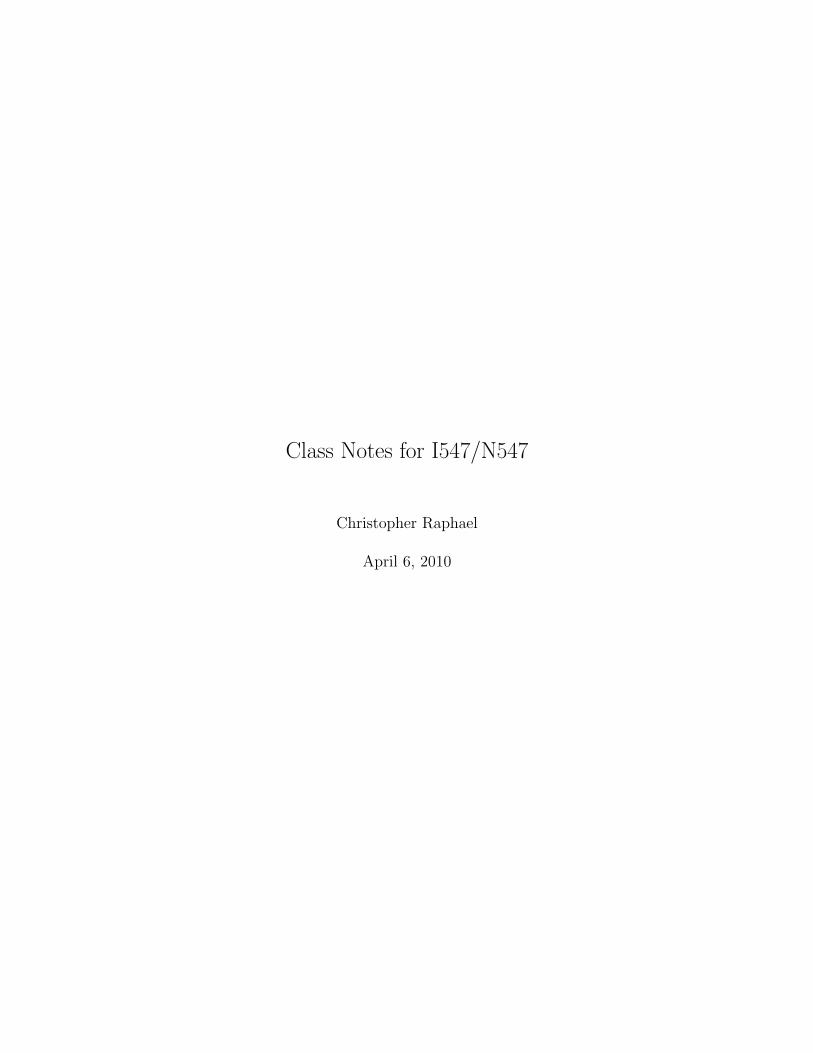
We could think of the projection as a function of the arc length traveled around the circle, rather than time. Thisprojection, as a function of the arc length traveled is the cosine function cos(t).
cos(t) = signed projection onto x axis after traveling arc length of t around unit circle
If we imagine the projection onto the y axis, analogously, we get the sine function.
(−1,0) (1,0)
(0,1)
(0,−1)
proj onto y axis
sin(t) = signed projection onto y axis after traveling arc length of t around unit circle
Note: since the projection onto the x axis starting at (1,0) (t = 0), is the same as the projection onto the y axisstarting at (0,1) t = π/2. we have cos(t) = sin(t+ π/2). That is, the sine and cosine functions are the same exceptfor a shift in time, as shown below:

6 CHAPTER 1. PRELIMINARIES
This discussion can be summarized in a single picture showing that the point on the unit circle making an angleof t with the x axis has coordinates (x = cos(t), y = sin(t)).
(cos(t),sin(t))
cos(t)
sin(t)
t
1.2.1 What Does Sine Sound Like? (simple sine.r)
A sine wave is a “pure” tone.
Frequency
sin(t) complete its cycle (period) every 2π (every trip around circle), so if t measures seconds, sin(2πt) oscillates onceevery second. Similarly, sin(2π2t) oscillates twice every second and
sin(2πft) oscillates f times per second.

1.2. THE SINE WAVE 7
We say that the frequency of sin(2πft) is f Hz = f cycles per second.Using the simple sine.r R program on the web page, listen to sine wave with the the following frequencies:
sin(2π440t) a sine at 440 Hz. This is the “A” that musicians often tune to.
sin(2π450t) a sine at 450 Hz. a little “higher” than before.
sin(2π430t) a sine at 430 Hz. a little “lower than before.
sin(2π880t) 880 = 2× 440 Hz. an octave above 440 Hz.
sin(2π1760t) 1760 = 2× 880 Hz. 2 octaves above 440 Hz.
Amplitude
The following figure shows sin(2πft) vs. 2 sin(2πft)
0 5 10 15
−2
−1
01
2
t
2 *
x
For positive a, a sin(2πft) oscillates between −a and +a. Construct the a sin(2πft) for a = 1, .1, .01, . . . usingthe simple sine.r program and listen to the sounds. You will hear the sounds becoming quieter and quieter.
Phase
The figure below shows a sin(2πft) vs a sin(2πft+ 1).

8 CHAPTER 1. PRELIMINARIES
0 5 10 15
−1.
0−
0.5
0.0
0.5
1.0
t
x
For any φ, a sin(2πft+ φ) is sine “shifted” earlier (to the left) by π radians. We will call φ the phase of the sinewave. Listen to a sin(2πft+ φ) for φ = 0, 1. There is no difference in the sound of the sine as we change the phase.
1.2.2 Periodicity
Have observed that sines at freqs. f and 2f sound similar (e.g. differ by octave). While we will never completelyexplain why this happens, we will observe some ways in which these two sine waves are similar from a mathematicalperspective.
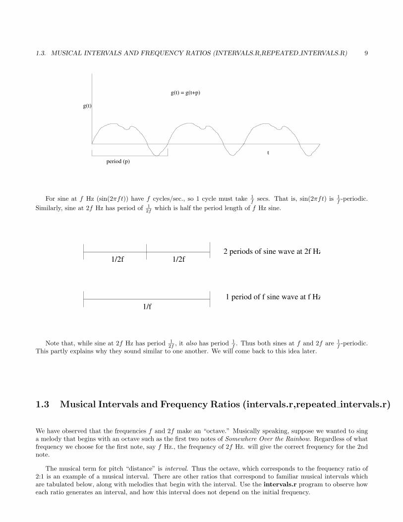
If a function repeats same shape over and over, it is said to be periodic. The period is the time for the functionto repeat. That is
g(t) = g(t+ p)
says that g is periodic with period p, or, more briefly, g is p-periodic. A an example of a periodic function is shownbelow.
1.3. MUSICAL INTERVALS AND FREQUENCY RATIOS (INTERVALS.R,REPEATED INTERVALS.R) 9
period (p)t
g(t)
g(t) = g(t+p)
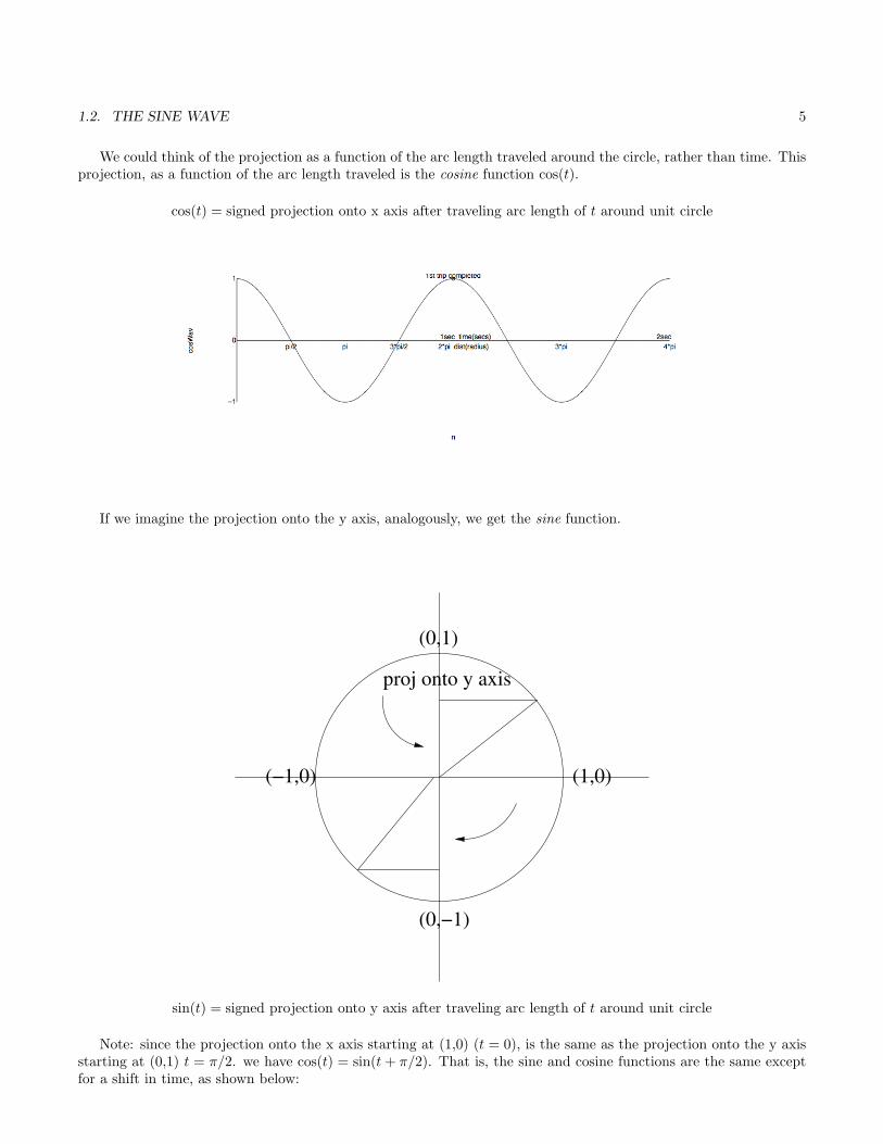
For sine at f Hz (sin(2πft)) have f cycles/sec., so 1 cycle must take 1f secs. That is, sin(2πft) is 1
f -periodic.Similarly, sine at 2f Hz has period of 1
2f which is half the period length of f Hz sine.
1/f
1/2f 1/2f
1 period of f sine wave at f Hz.
2 periods of sine wave at 2f Hz.
Note that, while sine at 2f Hz has period 12f , it also has period 1
f . Thus both sines at f and 2f are 1f -periodic.
This partly explains why they sound similar to one another. We will come back to this idea later.
1.3 Musical Intervals and Frequency Ratios (intervals.r,repeated intervals.r)
We have observed that the frequencies f and 2f make an “octave.” Musically speaking, suppose we wanted to singa melody that begins with an octave such as the first two notes of Somewhere Over the Rainbow. Regardless of whatfrequency we choose for the first note, say f Hz., the frequency of 2f Hz. will give the correct frequency for the 2ndnote.
The musical term for pitch “distance” is interval. Thus the octave, which corresponds to the frequency ratio of2:1 is an example of a musical interval. There are other ratios that correspond to familiar musical intervals whichare tabulated below, along with melodies that begin with the interval. Use the intervals.r program to observe howeach ratio generates an interval, and how this interval does not depend on the initial frequency.

10 CHAPTER 1. PRELIMINARIES
Ratio Interval Example2/1 (2:1) Octave Somewhere over the Rainbow3/2 (3:2) Perfect Fifth Also Sprach Zarathustra (a.k.a. theme from 2001)4/3 (4:3) Perfect Fourth Here comes the Bride5/4 (5:4) Major Third Kumbayah (1 2 3 in major)6/5 (6:5) Minor Third Chopin Funeral March (1 2 3 in minor)
Now consider the repeated intervals.r program. In this program we construct a sequence of sine waves begin-ning with an arbitrary frequency for the first note and getting the subsequent frequencies by multiplying the previousfrequency by the constant c = 1.414. What do we hear?
First note that every time we multiply the frequency by c the pitch moves up by the same interval. The musicalname for this interval is an augmented fourth. By the construction of the program, the frequencies of the notes mustbe
f, cf, c2f, c3f . . .
We can also hear that traversing two augmented 4ths brings us 1 octave above where we began (note that everyother note is the “same.”) Thus we have c2 = 2, hence c =
√2 ≈ 1.414. Thus multiplying a frequency by
√2 moves
the pitch up an augmented fourth.We could also let c = 3
√2 = 21/3 (the “third root” of 2). When we generate the series of pitches with frequencies
f, cf, c2f, c3f, . . . we hear that each note is a Major 3rd above its predecessor (remember Kumbayah: 3√
2 ≈ 5/4).We also see that traversing this interval 3 times brings us one octave above where we began since the frequencies aref, 21/3f, 22/3f, 23/3f = 2f, . . .. This follows from the rules for exponents since (21/3)k = 2k×1/3 = 2k/3. Thus theMajor 3rd splits the octave into 3 equal pieces.
If we continue this experiment dividing the octave into 4, 5, 6, . . . equal pieces we get
Ratio Interval Example21/2 Augmented 4th Maria or The Simpsons21/3 Major 3rd Kumbayah21/4 Minor 3rd (Chopin Funeral March or 1 2 3 in minor scale)21/5 #$%!& ugh!21/6 Major 2nd (1 2 in major scale)
Equal Temperament
Recall that the simple ratio for the major 3rd was 5/4. All things being equal, simple ratio intervals are oftenpreferred by musicians as the most “correct” tuning (more on this later). However, there is also a problem withsimple ratio intervals. Suppose we begin at a particular frequency and construct a series of pitches by moving up bya simple ratio major 3rd (by 5/4). In this case we have
f,54f,
2516f,
12564
f 6= 2f
If f corresponds to the note C, then we would get the notes C, E, G#, C, with the problem that the 2nd C is notquite twice the frequency of the first C.
Every scheme for generating a collection of frequencies for pitches following simple ratios runs up against aproblem of this kind. The most common answer to this problem is the notion of equal temperament (ET). The goalof equal temperament is to split the octave into 12 equal pieces. In Western music history the decision to divide theoctave into 12 pieces preceded the notion of equal temperament. Really, ET could be applied to any number of notesin the octave, though we will see an interesting connection between 12 and ET. We have learned that, in order to get

1.3. MUSICAL INTERVALS AND FREQUENCY RATIOS (INTERVALS.R,REPEATED INTERVALS.R) 11
12 equal musical intervals, we must have the same frequency ratio between each pair of frequencies. This is easilyaccomplished by the sequence:
f, 21/12f, 22/12f, 23/12f, . . . , 212/12f = 2f︸ ︷︷ ︸octave above f
where the initial frequency, f , is chosen arbitrarily (say A = 440 Hz).The main advantage of ET is that every “version” of the same interval (e.g. a minor third) sounds the same. For
instance, say
f︸︷︷︸C
, 21/12f︸ ︷︷ ︸C#
, 22/12f︸ ︷︷ ︸D
, 23/12f︸ ︷︷ ︸E[
, 24/12f︸ ︷︷ ︸E
, 25/12f︸ ︷︷ ︸F
, 26/12f︸ ︷︷ ︸F]
, . . .
Then we have
E[C
=23/12f
f= 23/12
EC]
=24/12f
21/12f= 23/12
FD
=25/12f
22/12f= 23/12
......
...
Of course, this argument holds for any interval, not just the minor third. A consequence of this tuning is that allthe different keys “sound” the same, as far as the intervals are concerned.
All of this discussion is based on the number the number 21/12 = 12√
2. It is often useful to know the value of thisconstant:
21/12 = 12√
2 ≈ 1.059
In other words, the frequencies of a half step (any half step) differ by about 6%. If you understand the argumentleading to ET tuning, then you also see, by identical reasoning, that your money will double in 12 years if compoundedat 6% annually.
Frequency vs. Midi
The Musical Instrument Digital Interface (MIDI) protocol associates a number with every possible musical pitch.The scheme assigns the numbers
......
...59 = B below middle C60 = middle C61 = C] above middle C
......
...
From this scheme we see that “tuning A” (A above middle C) is midi pitch 69. A common reference for this note isA = 440 Hz. If we let f(m) be the frequency of the ETT midi pitch using A = 440 Hz, we get
f(m) = 440× 2m−69
12
as a useful formula. From this formula we see that f(69) = 440 and that
f(m+ i)m
=440× 2
m+i−6912
440× 2m−69
12
= 2i12

12 CHAPTER 1. PRELIMINARIES
Simultaneous Sounds
= f(t) glass
CRASH!= g(t)
microphone
Consider the picture in which we have two sound sources:
1. A person singing f(t)
2. A glass falling of a table and breaking g(t)
Both sources generate sound (f(t) and g(t)) that will propagate through the room. If we measure the result of bothsounds at some point, say where the microphone is located, we get a signal h(t). How does h(t) relate to f(t) andg(t)?
Amazing Fact #1
h(t) = f(t) + g(t)
See the class web page for a demonstration of this.
Perfect Intervals (stability test.r)
We have observed that sine waves at frequencies f and 2f make an octave. We also have observed that both are1/f -periodic. Presumably the “simplicity” and “stability” of the octave comes from this shared periodicity. Theprogram stability test.r plays an interval followed by both notes sounding together. Use the program to see howintervals formed by simple ratios of integers (2:1, 3:1, 3:2, 4:3, etc.) sound stable and simple when played together.Why?
Consider sine waves at 2f and 3f .
• The sine at 2f has a period of 12f , but is also 1
f -periodic.
• The sine at 3f has a period of 13f , but is also 1
f -periodic.
So both have 1f periodicity leading to stability of the perfect fifth. Note that when the sines are summed (both
pitches played together) the sum is 1f -periodic
Similarly, sines at 3f and 4f both are 1f -periodic leading to the stability of the perfect fourth. The same argument
applies to other perfect intervals (though this terminology is not usual) such as 5/4 (major third) and 6/5 (minorthird).
1.3. MUSICAL INTERVALS AND FREQUENCY RATIOS (INTERVALS.R,REPEATED INTERVALS.R) 13
Clearly, from a musical standpoint as we look at the frequency ratio n+1n the interval becomes less stable. The
way to understand this is to keep the lower note fixed at freq. f , so the upper note is n+1n f . In this case
f = n× f
nn+ 1n
f = (n+ 1)× f
n
are both nf -periodic. So as n increases the length of the common period gets longer. It seems that it is the length of
this common period (the period of the sum) that relates to stability.
There is an interesting “dual” to this argument. If we keep the frequency ratio n+1n fixed (i.e. keep the musical
interval fixed) and let f decrease, the common period length, nf , increases. In other words. A fixed dyad (two notessounding at once) has a longer joint period as the lower note decreases. This corresponds to the conventional musicalwisdom that the same interval becomes increasing more “opaque” and “dissonant” as we go lower. While it may bedifficult to describe the way this sounds to us, this observation is the reason for the common way of voicing chordswith large intervals near the bottom and smaller ones near the top.
Relation to Equal Temperament (et beats.r)
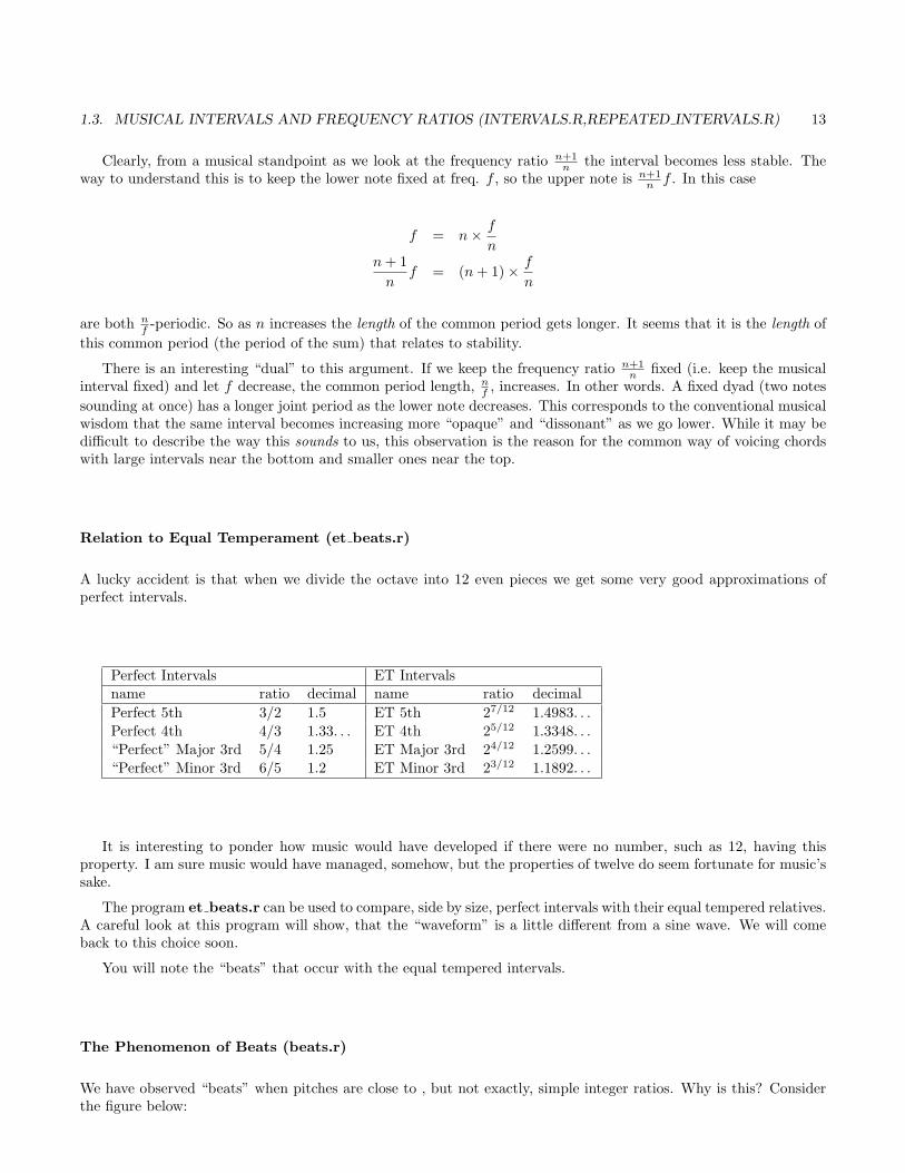
A lucky accident is that when we divide the octave into 12 even pieces we get some very good approximations ofperfect intervals.
Perfect Intervals ET Intervalsname ratio decimal name ratio decimalPerfect 5th 3/2 1.5 ET 5th 27/12 1.4983. . .Perfect 4th 4/3 1.33. . . ET 4th 25/12 1.3348. . .“Perfect” Major 3rd 5/4 1.25 ET Major 3rd 24/12 1.2599. . .“Perfect” Minor 3rd 6/5 1.2 ET Minor 3rd 23/12 1.1892. . .
It is interesting to ponder how music would have developed if there were no number, such as 12, having thisproperty. I am sure music would have managed, somehow, but the properties of twelve do seem fortunate for music’ssake.
The program et beats.r can be used to compare, side by size, perfect intervals with their equal tempered relatives.A careful look at this program will show, that the “waveform” is a little different from a sine wave. We will comeback to this choice soon.
You will note the “beats” that occur with the equal tempered intervals.
The Phenomenon of Beats (beats.r)
We have observed “beats” when pitches are close to , but not exactly, simple integer ratios. Why is this? Considerthe figure below:
14 CHAPTER 1. PRELIMINARIES
watch the dot
441 Hz
440 Hz
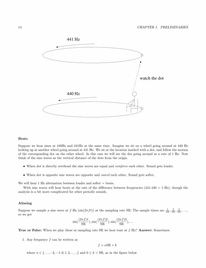
Beats
Suppose we hear sines at 440Hz and 441Hz at the same time. Imagine we sit on a wheel going around at 440 Hzlooking up at another wheel going around at 441 Hz. We sit at the location marked with a dot, and follow the motionof the corresponding dot on the other wheel. In this case we will see the dot going around at a rate of 1 Hz. Nowthink of the sine waves as the vertical distance of the dots from the origin.
• When dot is directly overhead the sine waves are equal and reinforce each other. Sound gets louder.
• When dot is opposite sine waves are opposite and cancel each other. Sound gets softer.
We will hear 1 Hz alternation between louder and softer = beats.With sine waves will hear beats at the rate of the difference between frequencies (441-440 = 1 Hz), though the
analysis is a bit more complicated for other periodic sounds.
Aliasing
Suppose we sample a sine wave at f Hz (sin(2πft)) at the sampling rate SR. The sample times are 1SR ,
2SR ,
3SR , . . . ,
so we get
sin((2πf)1
SR), sin(
(2πf)2SR
), sin((2πf)3
SR), . . .
True or False: When we play these at sampling rate SR we hear tone at f Hz? Answer: Sometimes.
1. Any frequency f can be written as
f = nSR + k
where n ∈ . . . ,−2,−1, 0, 1, 2, . . . , and 0 ≤ k < SR, as in the figure below

1.3. MUSICAL INTERVALS AND FREQUENCY RATIOS (INTERVALS.R,REPEATED INTERVALS.R) 15
2SRSR0 f
k
With f written this way the sampled values are
sin(
2π(nSR + k)1SR
), sin
(2π(nSR + k)2
SR
), sin
(2π(nSR + k)3
SR
), . . . ,
or, since the sine is 2π periodic,
sin(2πk1SR
), sin(2πk2SR
), sin(2πk3SR
), . . . ,
so f = nSR + k sounds the same as the frequency k:
nSR + k ⇐⇒ k
2. For f = SR− k get
sin(
2π(SR− k)1SR
), sin
(2π(SR− k)2
SR
), sin
(2π(SR− k)3
SR
), . . . ,
or
sin(2π(−k)1
SR), sin(
2π(−k)2SR
), sin(2π(−k)3
SR), . . . ,
soSR− k ⇐⇒ −k ⇐⇒︸︷︷︸
sin(−x)=− sin(x)
k
Thus the apparent frequency is given by
0
"true" frequency
apparentfrequency
SR/2 SR 2SR
SR/2

16 CHAPTER 1. PRELIMINARIES
Consequence: Can’t produce freq greater than SR/2 = “Nyquist” freq.
Since human hearing goes up to about 20 kHz a sampling of about 40 kHz (or 44.1 kHz) can represent the rangeof frequencies we can hear.
Sum of Sins and Periodicity (sum of sines.r, rand timbre.r)
If we add 2 sines waves differing by octave we get
g(t) = a1 sin(2πft+ φ1) + a2 sin(2π2ft+ φ2)
1/f
1/2f 1/2f
period of sine with freq f
2 periods of sine with freq 2f
1. Both sines are 1/f -periodic.
2. Sum of 1/f -periodic functions is 1/f -periodic.
so g(t) is 1/f -periodic. What do we hear?
1. Since the period of g(t) is 1/f we hear freq f .
2. Since the waveform is changed, we hear different tone color or timbre.
This is demonstrated in sum of sines.r. This idea generalizes to
g(t) = a1 sin(2πft+ φ1) + a2 sin(2π2ft+ φ2) + . . .+ an sin(2πnft+ φn)
Here, by similar reasoning, we still hear frequency f . This is demonstrated with the program rand timbre.r.This program creates sums of sine waves whose frequencies are integer multiples of some “base” frequency f . Theamplitudes of the sine waves are randomly chosen, as are the phases. You will hear that the sounds are all at thesame pitch, while the timbre changes.
Returning to the et beats.r program, recall that we observed beats for some “imperfect” intervals, such as theimperfect 5th associated with the ratio 27/12. In this example we create our tones by summing together sine wavesat integral multiples of the fundamental freqency, as described above. In the case of the imperfect 5th, since theratio is approximately 3/2, the 2nd harmonic of the higher note is almost the same frequency as the 3rd harmonic ofthe lower note. Thus we will hear beating between these sine waves.
Glissando
The 1st homework asked you to create a “pitch vibrato,” requiring a smooth transition over a range of frequencies.How do we do this?
We have observed that f(t) = sin(2πft) is a constant frequency at f Hz.

1.3. MUSICAL INTERVALS AND FREQUENCY RATIOS (INTERVALS.R,REPEATED INTERVALS.R) 17
Q: What is constant about sin(2πft)?
A: The “argument” to the sine, 2πft, has constant derivative:
d
dt2πft = 2πf = const.
We see in the above case that for sin(g(t)) the frequency at time t, f(t), is given by
f(t) =ddtg(t)2π
as described in the following figure:
g(t)
t2ff
If, for g(t) in this figure we take sin(g(t)) the frequency will double (jump an octave) when the rate of change(slope) of g(t) doubles.
The above equation holds more generally, however. For any function g(t), the sound sin(g(t)) will be a sine wavewhose pitch at time t is f(t) as above. Thus, if we want to create a function sin(g(t)) that has a certain time-varyingpitch, f(t), we just need to “undo” this equation by integrating:
g(t) = 2π∫ t
0
f(τ)dτ
Pitch Vibrato (pitch vibrato.r)
Suppose we want our frequency function to be
f(t) = f0 + ∆ sin(2πvt)
as would be appropriate for pitch vibrato. Here f0 is the base frequency we will move around, v is the rate of thevibrato in Hz., and ∆ is the width of the vibrato — that is the pitch will change in the range f0 ±∆. Our sound
18 CHAPTER 1. PRELIMINARIES
function will be sin(g(t)) where we get g(t) by integration as above:
g(t) = 2π(f0t−∆
2πvcos(2πvt)) = 2πf0t−
∆v
cos(2πt)
Thus our pitch vibrato is
s(t) = sin(2πf0t−∆v
cos(2πvt))
We can try this out with the program pitch vibrato.r.
Smooth Glissando (linear freq.r)
Suppose we want a sine tone with a linear increase in frequency:
f(t) = rt
To create this we want sin(g(t)) where we get g(t) by integrating the frequency function times 2π. That is,
g(t) = 2πr
2t2
so our sound function will be s(t) = sin(2π r2 t2). We can hear this sound with the program linear freq.r, though it
would be a good idea to try to predict what we will here first. The actual sound departs from expectation in twoways:
1. While the frequency increases at a constant rate, r, the musical pitch does not increase at a constant rate.This is because our perception of pitch difference is “logarithmic” — that is, to have constant pitch change,the frequency much change by a constant factor for each unit of time.
2. Of course, the pitch will not continue to go up and up, due to the aliasing issue we have introduced. Ratherwe will observe the triangular up and down motion frequency as we say when we first introduced the idea ofaliasing.
Uniform Glissando (uniform gliss.r)
Suppose we want to create a glissando that increases at a uniform rate in musical terms. To be definite, say we beginat frequency f0 at time t = 0 and rise one half step per second. In that case our frequency function, f(t), will have
f(0) = f020/12
f(1) = f021/12
f(2) = f022/12
......
...
To interpolate between these points in a smooth way we take
f(t) = f02t/12
which has exponential increase in frequency. More generally, say we wanted our frequency to traverse an octave everyT seconds. The our frequency function would be
f(t) = f02t/T
Using the usual integration argument, the associated sine function would be
sin(g(t)) = sin(2πf0T2t/T
log 2)
1.3. MUSICAL INTERVALS AND FREQUENCY RATIOS (INTERVALS.R,REPEATED INTERVALS.R) 19
f/2
f
2f
T
freq
1st harmonic
2nd harmonic
T
amp
1
1st harmonic
2nd harmonic
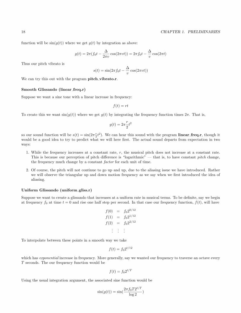
Figure 1.1: The evolution of frequencies (left) and amplitudes (right) of the two harmonics in the never-endingglissando.
Never-Ending Glissando (never ending gliss.r)
Suppose we construct a sound made up of two harmonics beginning at frequencies f0 and 2f0 as in the figure. Overthe course of T seconds both harmonics will drop one octave while retaining their precise 2:1 ratio. Thus, ratherthan appearing as two different sounds, we will hear a single sound whose timbre is richer than that of a sine wave.As this happens the amplitudes of these harmonics will also change, with the 1st harmonic decreasing linearly from1 to 0 while the 2nd harmonic increase from 0 to 1. The resulting sound will be given by h1(t) + h2(t) where
h1(t) = (1− t/T ) sin(−2πTf02−t/T
log 2)
h2(t) = (t/T ) sin(−2πT2f02−t/T
log 2)
This situation is illustrated in Figure 1.1. Observe the following
1. At t = 0 we have a single sine wave at frequency f0 with amplitude 1.
2. At t = T we have exactly the same situation.
Thus we could concatenate any number of copies of h1(t)+h2(t) to get a sound that appears to continually decreasewithout ever becoming low.
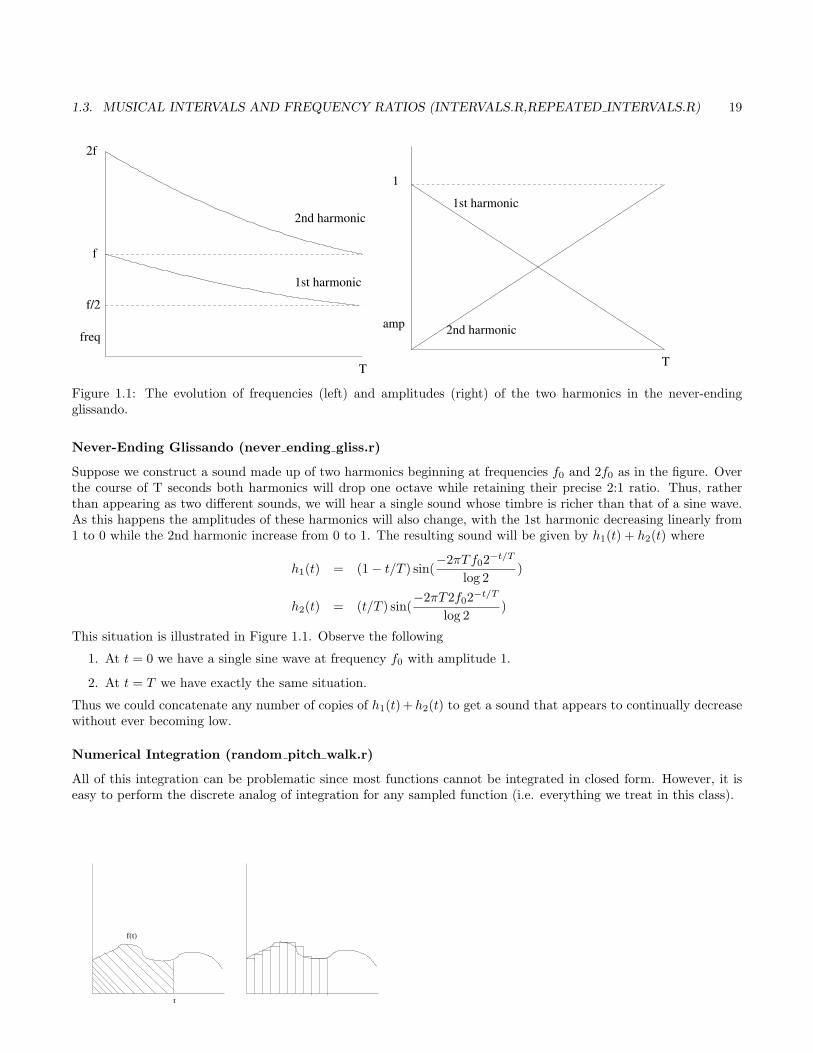
Numerical Integration (random pitch walk.r)
All of this integration can be problematic since most functions cannot be integrated in closed form. However, it iseasy to perform the discrete analog of integration for any sampled function (i.e. everything we treat in this class).
t
f(t)
20 CHAPTER 1. PRELIMINARIES
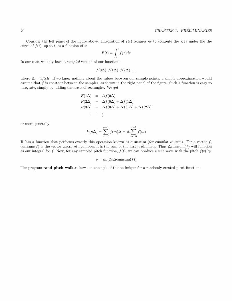
Consider the left panel of the figure above. Integration of f(t) requires us to compute the area under the thecurve of f(t), up to t, as a function of t:
F (t) =∫ t
0
f(τ)dτ
In our case, we only have a sampled version of our function:
f(0∆), f(1∆), f(2∆), . . .
where ∆ = 1/SR. If we knew nothing about the values between our sample points, a simple approximation wouldassume that f is constant between the samples, as shown in the right panel of the figure. Such a function is easy tointegrate, simply by adding the areas of rectangles. We get
F (1∆) = ∆f(0∆)F (2∆) = ∆f(0∆) + ∆f(1∆)F (3∆) = ∆f(0∆) + ∆f(1∆) + ∆f(2∆)
......
...
or more generally
F (n∆) =n−1∑m=0
f(m)∆ = ∆n−1∑m=0
f(m)
R has a function that performs exactly this operation known as cumsum (for cumulative sum). For a vector f ,cumsum(f) is the vector whose nth component is the sum of the first n elements. Thus ∆cumsum(f) will functionas our integral for f . Now, for any sampled pitch function, f(t), we can produce a sine wave with the pitch f(t) by
y = sin(2π∆cumsum(f))
The program rand pitch walk.r shows an example of this technique for a randomly created pitch function.

Chapter 2
Fourier Analysis
We have seen that
g(t) = a1 sin(2πft+ φ1) + a2 sin(2π2ft+ φ2) + . . .+ an sin(2πnft+ φn)
is periodic with period 1/f so g(t) sounds at f Hz. As we varied the amplitudes a1, . . . , an we saw that the timbreor color of the sound changed.
Amazing Fact #2
Any 1f -periodic function, g(t), can be approximated as well as we like by
g(t) ≈ a1 sin(2πft+ φ1) + a2 sin(2π2ft+ φ2) + . . .+ an sin(2πnft+ φn)
by choosing the number of terms, n, and the coefficients, a1, . . . , an and the phases φ1, . . . , φn appropriately. Infact, if t takes only a finite number of values, 0
SR ,1SR , . . . ,
N−1SR then the approximating in the equation becomes an
equality.
Q: How do we get the a’s and the φ’s?
A: Fourier Analysis
Complex Numbers
Re
Im z
Re(z)
Im(z)
Arg(z)
Mod(z)
−i
i
1−1
21

22 CHAPTER 2. FOURIER ANALYSIS
Complex numbers are numbers z = a + bi where i =√−1. Students first encountering complex numbers often
question the use of such numbers which don’t seem to represent anything familiar in the world we know. Just asnegative numbers have natural interpretations in terms of debt (having a negative amount of money) or position (+in one direction and - in the opposite), complex numbers have concrete interpretations in some cases. One of themost compelling of these is the subject we are about to study.
Complex numbers can be visualized as points in the complex plane where the horizontal axis denotes the realpart of the number and the vertical axis denotes the imaginary part. That is, if z = a+ bi is a complex number thenthe point with coordinates (a, b) is the graphical representation of z. A complex number has 4 attributes that willbe important to us. The “real part” of z is denoted by Re(z). With z as above Re(z) = a. Similarly the “imaginarypart” of z, Im(z) = b (the imaginary part is a real number). A complex number, z makes an angle with the realaxis which we denote as Arg(z) and has a length Mod(z) =
√a2 + b2. These quantities are illustrated in the figure
above. The R program handles complex numbers and uses the same notation of Re,Im,Mod,Arg.We will occasionally refer to the polar representation of a complex number. Suppose we define eiθ as the number
on the unit circle of the complex plane making angle θ with the real axis, as in the figure below. This may not seemlike it has anything to do with the familiar view of the exponential function, so just take it as a definition for now.If we multiply this number by a real constant r, then reiθ “points” in the same direction as eiθ but has length r. Inother words, if z is a complex number with Mod(z) = r and Arg(z) = θ, then z = reiθ. Sometimes this is called the“polar” representation of z, since it is essentially polar coordinates.
e
θ
i θ
e i θr
One can do many things with complex numbers that we are used to doing with real numbers. For instance,complex numbers can be added, just like two dimensional vectors. That is, if z1 = a1 + b1i and z2 = a2 + b2i thenz1 + z2 = (a1 +a2)+ (b1 + b2)i. More unusual is multiplication for complex numbers, which is most intuitive in polarform. If z1 = r1e
iθ1 , and z2 = r2eiθ2 then z1z2 = r1r2e
i(θ1+θ2). Note that the moduli are multiplied while the anglesare added. Thus the familiar rule of exey = ex+y holds for complex numbers too.
Adding Sines of Identical Frequency
Some kinds of calculations are easier with complex numbers. Here is an example. Suppose you have two cosines atthe same frequency, f , but with different amplitudes and phases: a1(t) = a1 cos(2πft + φ1) and a2 cos(2πft + φ2).

23
What is the result when we add these together. In polar complex notation we have
a1 cos(2πft+ φ1) + a2 cos(2πft+ φ2) = Re(a1e2πift+iφ1) + Re(a2e
2πift+iφ2)= Re(a1e
2πift+iφ1 + a2e2πift+iφ2)
= Re((a1eiφ1 + a2e
iφ2)e2πift)= Re(aeiφe2πift)= a cos(2πft+ φ)
In words, we add the complex numbers a1eiφ1 and a2e
iφ2 associated with the amplitudes and phases of the originalcosines. The result, expressed in polar form, gives the amplitude and phase of the resulting cosine. Note that theresult has the same frequency f . See the figure below:
a e
a e
a eip
11
2ip
2
ip
Finite Fourier Transform
Suppose we have a sampled function (a waveform) consisting of N points, f(0), f(1), . . . , f(N − 1) where N is even.We will represent f as a sum of cosine waves that oscillate 0, 1, . . . , N/2 times over the N points. Examples of suchcosine function are given in Figure 2.1. Note that the cosine that oscillates 0 times is just function that is identicallyequal to 1, while the cosine that oscillates N/2 times alternates back and forth between 1 and -1.
To be precise, we will use the functions cn(j) for n = 0, 1, . . . , N/2 defined by
cn(j) = cos(2πnjN
)
for j = 0, 1, . . . , N − 1. In representing f we will allow the shifting and scaling of these functions. That is, we let
cn,an,φn(j) = an cos(
2πnjN
+ φn)
for j = 0, 1, . . . , N − 1. Then we represent f as
f = c0,a0,φ0 + c1,a1,φ1 + . . .+ cN/2,aN/2,φN/2
=N/2∑n=0
cn,an,φn
for some collection of amplitudes an and phase shifts φn. Pictorially, this is represented as follows

24 CHAPTER 2. FOURIER ANALYSIS
0 1 2 3 4 5 6
−1.0
−0.5
0.0
0.5
1.0
0 1 2 3 4 5 6
−1.0
−0.5
0.0
0.5
1.0
0 1 2 3 4 5 6
−1.0
−0.5
0.0
0.5
1.0
0 1 2 3 4 5 6
−1.0
−0.5
0.0
0.5
1.0
0 1 2 3 4 5 6
0.6
0.8
1.0
1.2
1.4
0 1 2 3 4 5 6
−1.0
−0.5
0.0
0.5
1.0
Figure 2.1: The discrete cosine vectors used in representing an N -point function (waveform). Pictures in “reading”order are the cosines that oscillate 1,2,3,4,0, and N/2 times. Note that the cosine that oscillates 0 times is justconstant at 1, while the one the oscillates N/2 times oscillates back and forth between 1 and -1.

25
!"# $%&' ()*+,-./ 0123 4567 89:; <=>? @ABC DEFG HIJK LMNO PQRS TU
VWXYZ[\]^_`abcdefghijklmnopqrstuvwxyz|
~ ¡¢£ ¤¥¦§¨©ª« ¬®¯ °±²³ ´µ¶· ¸¹º» ¼½¾¿ ÀÁÂà ÄÅ ÆÇÈÉ ÊËÌÍ ÎÏÐÑ
ÒÓ
0th cosine (constant)
1st cosine (oscillates once)
2nd cosine (oscillates twice)
N/2th cosine (alternates)
=+
f
The key to getting this representation is the Finite Fourier Transform (FFT).
Definition of FFT
In this document we abbreviate the Finite Fourier Transform as FFT. “FFT” is also commonly used as an abbreviationfor “Fast Fourier Transform” which is an algorithm that is used to implement the Finite Fourier Transform. Sinceboth refer to the same mathematical construction, if there is any confusion it is usually harmless.
The FFT of f = (f(0), . . . , f(N − 1)), is a complex-valued N -vector F = (F (0), F (1), . . . , F (N − 1)) given by
F (n) =N−1∑j=0
f(j)e−2πinj
N
for n = 0, 1, . . . , N − 1. We will denote the relationship between a f and its finite Fourier transform, F , as
fFFT←→ F
We will come back to this definition later, but first let’s discuss its consequences.
Interpretation of FFT
If f = (f(0), f(1), . . . , f(N − 1)) and F is the FFT of f :
fFFT←→ F
then we can recover the amplitudes and phases of the cosines used in our reconstruction of f . That is
φn = Arg(F (n))
an =
Mod(F (n))
N/2 for n = 1, . . . , N/2− 1Mod(F (n))
N for n = 0, N/2
FFT in R
R computes the FFT of an N -vector, f , as
> F = fft(f);
Each of the N components of F is a complex number. R handles complex numbers in a wide variety of calculations,and nearly any calculation where complex numbers make sense such as addition, multiplication, etc. Usually, if oneis going to plot the complex numbers corresponding to the FFT it is better to plot some real-valued attribute suchas their amplitude, (Mod(F)), or phases, (Arg(F)). While R can compute an FFT for any length vector, the FFTalgorithm works most efficiently when the length is a power of 2. We will always choose this length to be a power of2, since it costs us nothing.
Due to the 1-based indexing of the R program, F (n) for n = 1, . . . , N gives the phase and amplitude for thecosine that oscillates n − 1 times in N points. This is yet another argument for the inferiority of 1-based indexing,but the issue is easy enough to deal with.

26 CHAPTER 2. FOURIER ANALYSIS
Understanding the Meaning of the FFT (sine id 1.r,sine id 2.r, sawtooth.r)
As a first example we will construct a function which we know consists of a single cosine using the R programsine id 1.r. This program allows one to vary the frequency and phase of the cosine, though the frequency (inoscillations per N points) must be integral. When we compute the FFT of this one-cosine function, all values of theFFT are 0 = 0 + 0i except for the component corresponding to our cosine. That is, if our cosine is at frequency n,then only F (n+ 1) will be nonzero. We then can recover the amplitude and phase as
> amp = Mod(F(n+1))/(N/2)> ph = Arg(F(n+1))
The program sine id 2.r does the same thing, but now we take a function formed as the sum of 3 such cosines,again with integral frequency, having different amplitude and phase. Looking at a plot of this function, as theprogram does, it is hard for us to imagine how it was constructed, but the FFT has no difficulty in “resolving” thefunction into its constituent cosines. Again the three FFT components “light up” and from these we can recover theamplitudes and phases as before.
The R program sawtooth.r shows a more interesting example. In this case we can take f to be any N -pointfunction we want, such as a sawtooth waveform, or even something generated in a random fashion. The programloops through all possible frequencies, from 0, to N/2, and adds in the appropriate cosine wave for the currentfrequency, scaled and shifted as prescribed by the appropriate FFT component. Reading directly from the code, thisis accomplished by
> yhat = yhat + Mod(Y[i])*cos((i-1)*t + Arg(Y[i])) # add in new cosine
In this example yhat is the “accumulator” that holds the sum from the “currently visited” frequencies. In this lineof code we add to the accumulator the scaled and shifted cosine which oscillates i− 1 times (remember the 1-basedindexing of R). Each time through the loop we display the current approximation to our target function. As we movethrough the iterations we can see the approximation getting better and better until it is indistinguishable from thetarget.
The two examples in the program — the “sawtooth” function and the randomly generated function show twodifferent views of the FFT. In the first example we take a periodic function which is a “sawtooth” or up and downtriangle shape. We use the FFT to represent a single period of this function in terms of sine waves that oscillateintegral numbers of times over the period. For those familiar with the idea of the “Fourier Series,” this is a discreteapproximation of the series. The next example takes a randomly generated function. It seems rather odd to thinkof this as a period of pitched sound, though we could view it that way. If we regard it as a generic wave form(not necessarily periodic), we see that we can still approximate it in terms of cosines. Thus, the FFT works as adecomposition for any discrete function, such as a sound file.
Arbitrary Sine Waves (arbitrary sine.r)
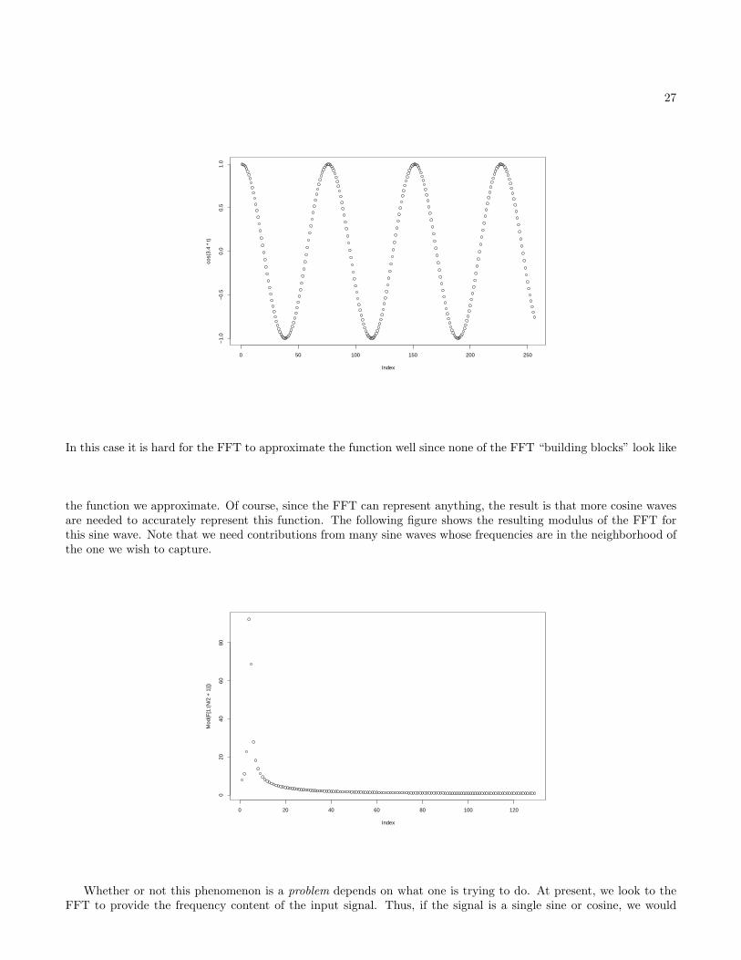
The FFT represents a waveform in terms of cosines that oscillate an integral number of times per FFT-length. Whatif we analyze a sine or cosine that doesn’t “match” any of our FFT frequencies, as in the following figure? Note that,over the 256 points we will examine (our FFT length) the sine wave ends up with a different phase than it starts with.
27
0 50 100 150 200 250
−1.
0−
0.5
0.0
0.5
1.0
Index
cos(
3.4
* t)
In this case it is hard for the FFT to approximate the function well since none of the FFT “building blocks” look like
the function we approximate. Of course, since the FFT can represent anything, the result is that more cosine wavesare needed to accurately represent this function. The following figure shows the resulting modulus of the FFT forthis sine wave. Note that we need contributions from many sine waves whose frequencies are in the neighborhood ofthe one we wish to capture.
0 20 40 60 80 100 120
020
4060
80
Index
Mod
(F[1
:(N
/2 +
1)]
)
Whether or not this phenomenon is a problem depends on what one is trying to do. At present, we look to theFFT to provide the frequency content of the input signal. Thus, if the signal is a single sine or cosine, we would

28 CHAPTER 2. FOURIER ANALYSIS
like to see this more accurately reflected in the FFT. We can accomplish this by windowing the data — multiplyingour input by a function that trails off to zero at both endpoints. There are many possible choices of windows and ahuge amount of literature on the effects of this choice. This topic will not concern us in this class, so we will use thecommon “Hann,” or “raised cosine” window for all of our experiments. This window is given by
h(j) =1 + cos( 2πj
N − π)2
j = 0, . . . , N −1. and is depicted below. Superimposed on the figure is the effect of multiplying the signal consideredabove with the Hann window.
0 50 100 150 200 250
−1.
0−
0.5
0.0
0.5
1.0
Index
hann
* f
Finally, we show below the effect on the FFT. Note that the frequency content is less spread out, which is moreconsistent with our perception of this signal.
0 20 40 60 80 100 120
010
2030
4050
60
Index
Mod
(F[1
:(N
/2 +
1)]
)
29
Usually real-audio samples are windowed before Fourier transforms are taken.
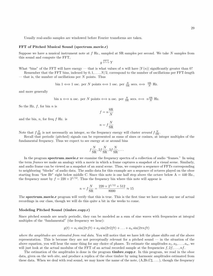
FFT of Pitched Musical Sound (spectrum movie.r)
Suppose we have a musical instrument note at f Hz., sampled at SR samples per second. We take N samples fromthis sound and compute the FFT,
yFFT←→ Y
What “bins” of the FFT will have energy — that is what values of n will have |Y (n)| significantly greater than 0?Remember that the FFT bins, indexed by 0, 1, . . . , N/2, correspond to the number of oscillations per FFT-length
— that is, the number of oscillations per N points. Thus
bin 1⇐⇒ 1 osc. per N points⇐⇒ 1 osc. per NSR secs.⇐⇒ SR
N Hz.
and more generally
bin n⇐⇒ n osc. per N points⇐⇒ n osc. per NSR secs.⇐⇒ nSR
N Hz.
So the Hz, f , for bin n is
f = nSRN
and the bin, n, for freq f Hz. is
n = fN
SRNote that f N
SR is not necessarily an integer, so the frequency energy will cluster around f NSR .
Recall that periodic (pitched) signals can be represented as sums of sines or cosines, at integer multiples of thefundamental frequency. Thus we expect to see energy at or around bins
fN
SR, 2f
N
SR, 3f
N
SR, . . .
In the program spectrum movie.r we examine the frequency spectra of a collection of audio “frames.” In usingthe term frames we make an analogy with a movie in which a frame captures a snapshot of a visual scene. Similarly,and audio frame can be viewed as a snapshot of an aural scene. Thus, we compute a sequence of FFTs correspondingto neighboring “blocks” of audio data. The audio data for this example are a sequence of octaves played on the oboestarting from “low B[” right below middle C. Since this note is one half step above the octave below A = 440 Hz.,the frequency must by f = 220× 21/12. Thus the frequency bin where this note will appear is
n = fN
SR=
220× 21/12 × 5128000
≈ 15
The spectrum movie.r program will verify that this is true. This is the first time we have made any use of actualrecordings in our class, though we will do this quite a bit in the weeks to come.
Modeling Pitched Sound (timbre copy.r)
Since pitched sounds are nearly periodic, they can be modeled as a sum of sine waves with frequencies at integralmultiples of the “fundamental” (the frequency we hear):
g(t) = a1 sin(2πft) + a2 sin(2π2ft) + . . .+ an sin(2πnft)
where the amplitudes are estimated from real data. You will notice that we have left the phase shifts out of the aboverepresentation. This is because they are not perceptually relevant for a pitched sound — in the situation of theabove equation, you will hear the same thing for any choice of phases. To estimate the amplitudes a1, a2, . . . , an, wewill just look at the actual modulus of the FFT of an actual recorded sample at the frequencies f, 2f, . . . , nf .
The estimation of the amplitudes is done in the program timbre copy.r. In this program, we read in the oboedata, given on the web site, and produce a replica of the oboe timbre by using harmonic amplitudes estimated fromthese data. When we deal with real sound, we may know the name of the note, (A,B[,C], . . . ), though the frequency
30 CHAPTER 2. FOURIER ANALYSIS
is only known approximately. Thus, the program looks at a range of FFT “bins” in the neighborhood of the positionwhere each harmonic (multiple of the fundamental f ) should lie. For the kth harmonic, we estimate ak to be
ak = maxn∈N(kf)
|G(n)|
where N(kf) is a neighborhood of the kth harmonic (± 3 bins in the program) and G is the FFT of our sound g.We would get similar sounding results if we looked at the sum of the |G(n)| over each neighborhood, or, perhaps,√∑
|G(n)|2In performing this estimation we have created a simple model for the data. Model-based approaches are flexible:
we can apply this model to other notes, produce notes of any length, add vibrato and glissando, etc. Consider thisapproach as compared to one that works directly with the sampled sound. A purely sample-based approach is muchmore limited, since it can only play the exact samples back (with minor modifications) and can thus create only asmall range of variation.
Noise (white noise.r, colored noise.r)
We can think of noise as sound that is not pitched, and thus has no “singable” tone — more formal definitions arepossible, of course, nearly all involving some notion of randomness in the data. The Fourier transform can also beused to capture the perceptual characteristics of noisy sounds, as well as pitched sounds.
When samples are chosen randomly and independently the result is often deemed “white” noise. While we willnot define “independence” in a formal sense here, we mean that each sample is chosen without regard for the othersamples, as would be the case with a random number generator. The term “white” is used in analogy with light.When all frequencies of light are present, as in light that comes from the sun, the light looks white in color. Wecan see from the program white noise.r that independent random numbers produce energy at at all frequencies,though the contribution at each frequency is random. The program also plays the associated sound, which soundssomething like the ocean, or a huge volume of rushing water.
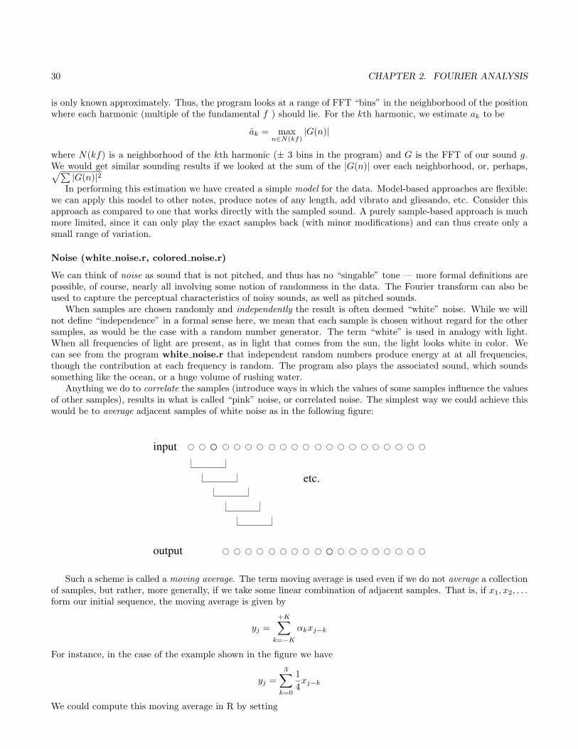
Anything we do to correlate the samples (introduce ways in which the values of some samples influence the valuesof other samples), results in what is called “pink” noise, or correlated noise. The simplest way we could achieve thiswould be to average adjacent samples of white noise as in the following figure:
!!""##$$ %%&&''(())** ++,,
--..//00 11223344 55667788 99::;;<< ==>>??@@AABB CCDDEEFF GGHHIIJJ KKLLMMNNOOPPQQRR
etc.
output
input
Such a scheme is called a moving average. The term moving average is used even if we do not average a collectionof samples, but rather, more generally, if we take some linear combination of adjacent samples. That is, if x1, x2, . . .form our initial sequence, the moving average is given by
yj =+K∑
k=−K
αkxj−k
For instance, in the case of the example shown in the figure we have
yj =3∑k=0
14xj−k
We could compute this moving average in R by setting
31
> N = 8192> x = rnorm(N)> y = rep(0,N)> for (j in 1:N-4) y[j] = mean(x[j:(j+4)]);
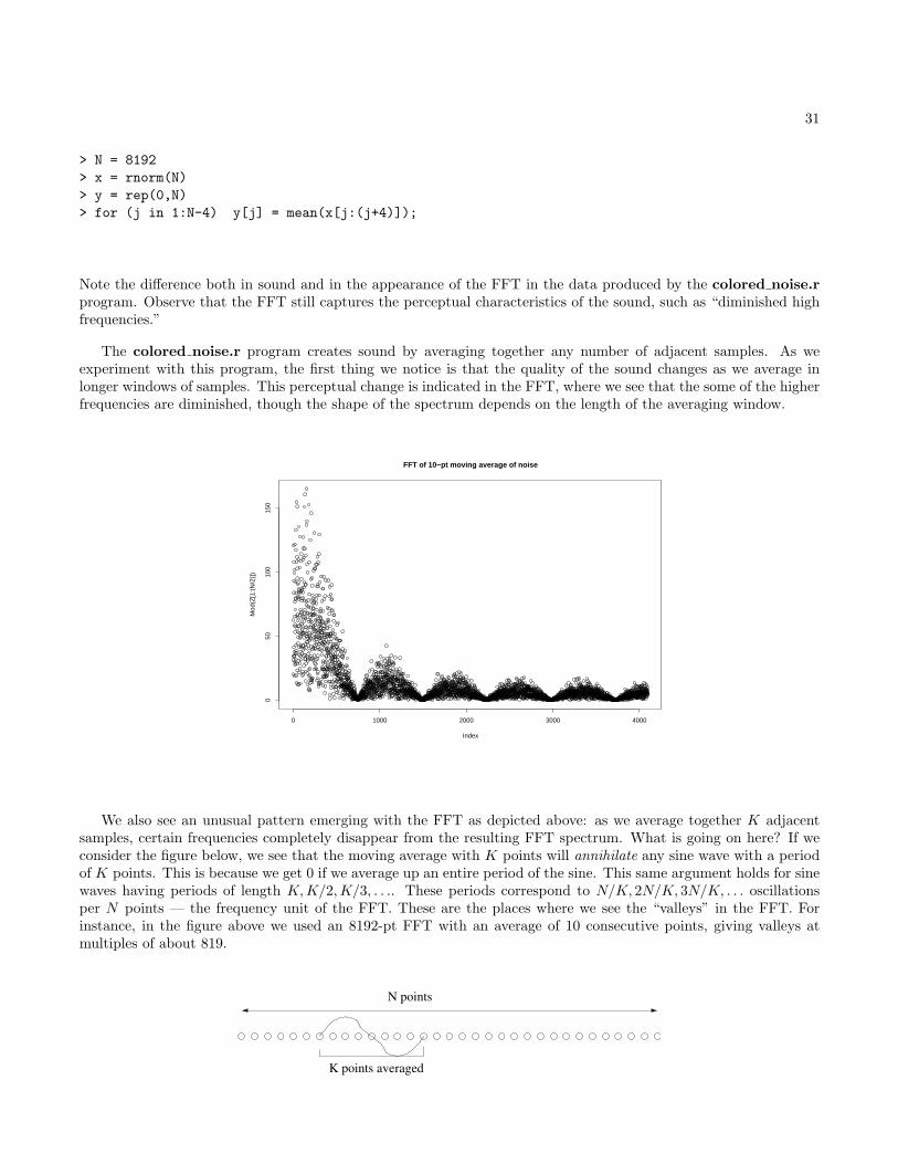
Note the difference both in sound and in the appearance of the FFT in the data produced by the colored noise.rprogram. Observe that the FFT still captures the perceptual characteristics of the sound, such as “diminished highfrequencies.”
The colored noise.r program creates sound by averaging together any number of adjacent samples. As weexperiment with this program, the first thing we notice is that the quality of the sound changes as we average inlonger windows of samples. This perceptual change is indicated in the FFT, where we see that the some of the higherfrequencies are diminished, though the shape of the spectrum depends on the length of the averaging window.
0 1000 2000 3000 4000
050
100
150
FFT of 10−pt moving average of noise
Index
Mod
(Z[1
:(N
/2)]
)
We also see an unusual pattern emerging with the FFT as depicted above: as we average together K adjacentsamples, certain frequencies completely disappear from the resulting FFT spectrum. What is going on here? If weconsider the figure below, we see that the moving average with K points will annihilate any sine wave with a periodof K points. This is because we get 0 if we average up an entire period of the sine. This same argument holds for sinewaves having periods of length K,K/2,K/3, . . .. These periods correspond to N/K, 2N/K, 3N/K, . . . oscillationsper N points — the frequency unit of the FFT. These are the places where we see the “valleys” in the FFT. Forinstance, in the figure above we used an 8192-pt FFT with an average of 10 consecutive points, giving valleys atmultiples of about 819.
!!""##$$ %%&&''(( ))**++,, --..//00 11223344 55667788 99::;;<< ==>>??@@ AABB
N points
K points averaged

32 CHAPTER 2. FOURIER ANALYSIS
Filtering
Suppose we have two vectors, a “long” one, x = (x0, x1, . . . , xN−1) and a “short” one a = (a0, . . . , aL). We can usethe vector a to generate a new sequence from x called y, by letting
yj = a0xj + a1xj−1 + a2xj−2 + . . . , aLxj−L
A simple example of this is the “averaging” operation we have already seen. In this case a = ( 1L+1 ,
1L+1 , . . . ,
1L+1 ).
This operation is known as filtering, convolution, or moving average. As notation for this operation we will write
y = a ∗ x
where
(a ∗ x)(j) =L∑l=0
alxj−l (2.1)
=∑
(l,k):l+k=j
alxk (2.2)
The filtering operation has an interesting relation to the FFT, as follows:
Amazing Fact # 3
If we are careful in the definition of the filtering operation, the effect of filtering in the “time domain” by a is thatof multiplying by the FFT of a in the “frequency domain.” That is, if x FFT←→ X and a FFT←→ A then
a ∗ x FFT←→ A ·X (2.3)
A little care is needed in interpreting this equation. Since we are dealing with the finite Fourier transform here,we must be more precise about the meaning of the convolution. In particular, we need a “circular” convolution.The definition of the circular convolution is almost identical to the one already presented. The difference is thatwe interpret the addition and subtraction in 2.1 and 2.2 as being modulo N (remainder when divided by N), whereN is the length of the sequences. In these equations we treat a also as an N -length sequence where most of thecomponents of a may be 0. While it is circular convolution that transforms exactly into the product of the Fouriertransforms, this is approximately true if we don’t bother with the circular aspect of the convolution.

33
!
"#$% &'
()*+,-./0123
N−2N−1 0 1
2
x
amultiply and add ....
While we don’t emphasize the mathematical aspects of this course, the convolution relation of Eqn. 2.3 is easyto verify as follows:
FFT(a ∗ x)(n) =N−1∑j=0
(a ∗ x)je−2πijn
N
=N−1∑j=0
∑l+k=j
alxke−2πijn
N
=N−1∑l=0
N−1∑k=0
alxke−2πiln
N e−2πikn
N
=N−1∑l=0
ale−2πiln
N
N−1∑k=0
xke−2πikn
N
= A(n)X(n)
Understanding Filtering (noise filter.r)
Let’s consider applying the averaging filter
a = (1L,1L, . . . ,
1L
)︸ ︷︷ ︸L components
to some white noise, x, as before, with xFFT←→ X. We have already seen that white noise has a flat (and random)
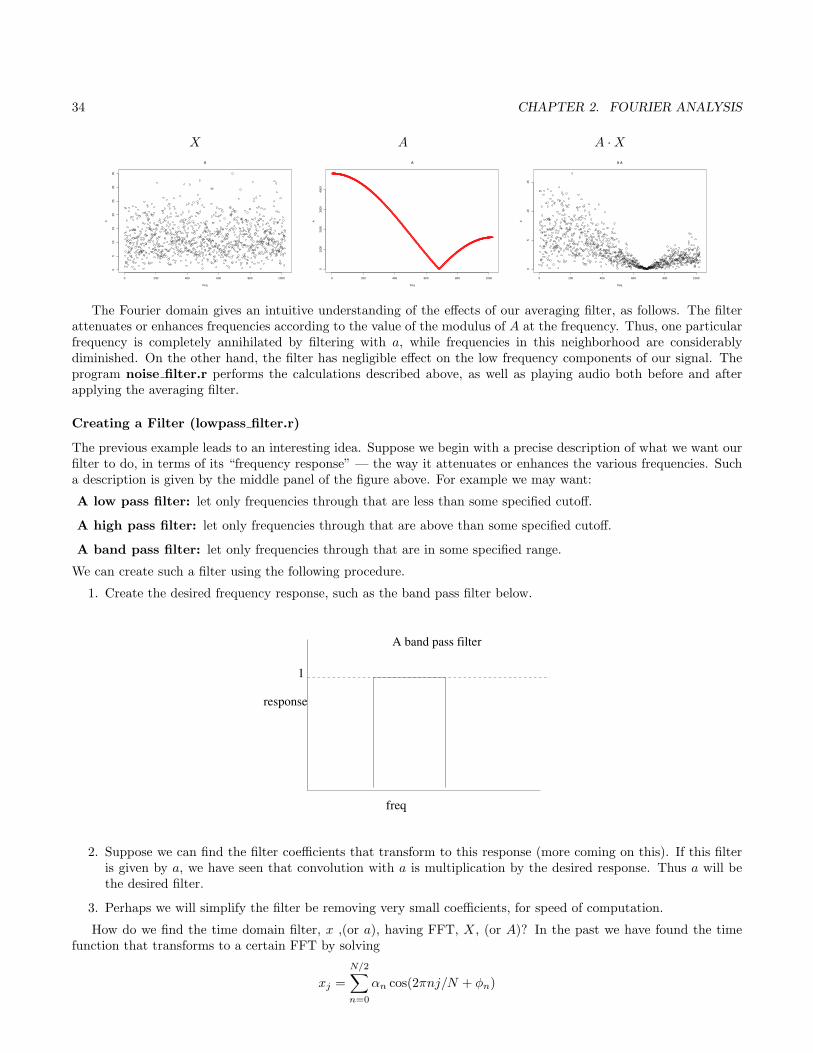
spectrum, as in the left panel of the figure below. The middle panel of the figure shows the modulus of A — thetransform of our filter, a. In constructing A we simply “pad” a with zeros to make it the same length as x beforetransforming — this corresponds to the identical filter operation, but leaves A comparable with X. We have learnedthe effect of filtering (convolving) the noise, x, with our averaging filter, a, in frequency domain is the product A ·X,as given in the right panel of the figure.
34 CHAPTER 2. FOURIER ANALYSIS
X A A ·X
0 200 400 600 800 1000
05
1015
2025
3035
X
freq
X
0 200 400 600 800 1000
010
0020
0030
0040
00
A
freq
A
0 200 400 600 800 1000
05
1015
X A
freq
Z
The Fourier domain gives an intuitive understanding of the effects of our averaging filter, as follows. The filterattenuates or enhances frequencies according to the value of the modulus of A at the frequency. Thus, one particularfrequency is completely annihilated by filtering with a, while frequencies in this neighborhood are considerablydiminished. On the other hand, the filter has negligible effect on the low frequency components of our signal. Theprogram noise filter.r performs the calculations described above, as well as playing audio both before and afterapplying the averaging filter.
Creating a Filter (lowpass filter.r)
The previous example leads to an interesting idea. Suppose we begin with a precise description of what we want ourfilter to do, in terms of its “frequency response” — the way it attenuates or enhances the various frequencies. Sucha description is given by the middle panel of the figure above. For example we may want:
A low pass filter: let only frequencies through that are less than some specified cutoff.
A high pass filter: let only frequencies through that are above than some specified cutoff.
A band pass filter: let only frequencies through that are in some specified range.
We can create such a filter using the following procedure.
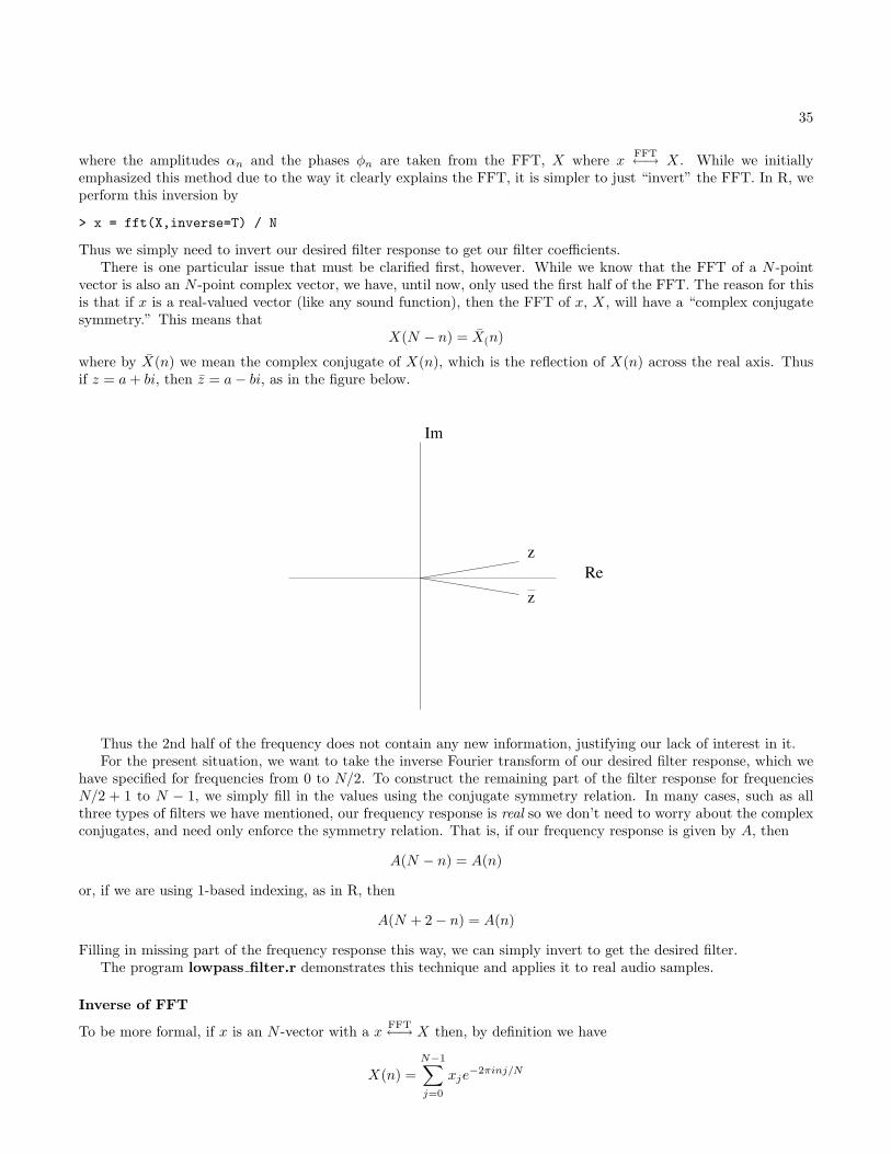
1. Create the desired frequency response, such as the band pass filter below.
freq
response
1
A band pass filter
2. Suppose we can find the filter coefficients that transform to this response (more coming on this). If this filteris given by a, we have seen that convolution with a is multiplication by the desired response. Thus a will bethe desired filter.
3. Perhaps we will simplify the filter be removing very small coefficients, for speed of computation.
How do we find the time domain filter, x ,(or a), having FFT, X, (or A)? In the past we have found the timefunction that transforms to a certain FFT by solving
xj =N/2∑n=0
αn cos(2πnj/N + φn)
35
where the amplitudes αn and the phases φn are taken from the FFT, X where xFFT←→ X. While we initially
emphasized this method due to the way it clearly explains the FFT, it is simpler to just “invert” the FFT. In R, weperform this inversion by
> x = fft(X,inverse=T) / N
Thus we simply need to invert our desired filter response to get our filter coefficients.There is one particular issue that must be clarified first, however. While we know that the FFT of a N -point
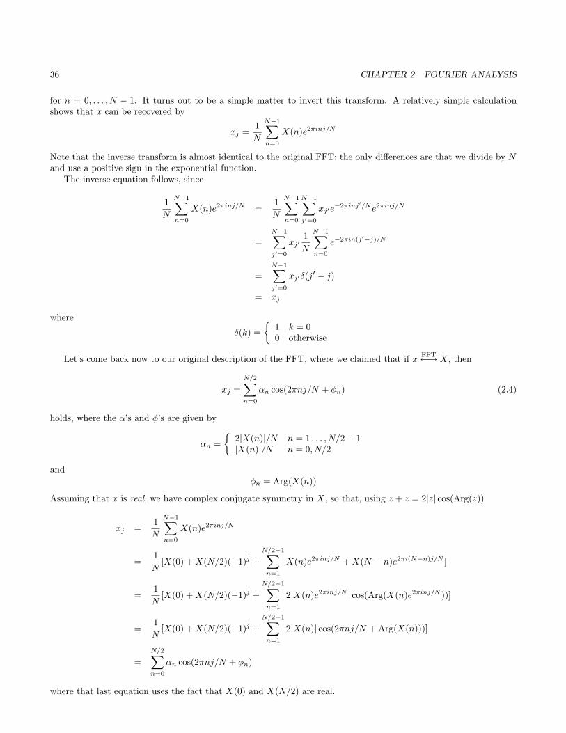
vector is also an N -point complex vector, we have, until now, only used the first half of the FFT. The reason for thisis that if x is a real-valued vector (like any sound function), then the FFT of x, X, will have a “complex conjugatesymmetry.” This means that
X(N − n) = X(n)
where by X(n) we mean the complex conjugate of X(n), which is the reflection of X(n) across the real axis. Thusif z = a+ bi, then z = a− bi, as in the figure below.
z
zRe
Im
Thus the 2nd half of the frequency does not contain any new information, justifying our lack of interest in it.For the present situation, we want to take the inverse Fourier transform of our desired filter response, which we
have specified for frequencies from 0 to N/2. To construct the remaining part of the filter response for frequenciesN/2 + 1 to N − 1, we simply fill in the values using the conjugate symmetry relation. In many cases, such as allthree types of filters we have mentioned, our frequency response is real so we don’t need to worry about the complexconjugates, and need only enforce the symmetry relation. That is, if our frequency response is given by A, then
A(N − n) = A(n)
or, if we are using 1-based indexing, as in R, then
A(N + 2− n) = A(n)
Filling in missing part of the frequency response this way, we can simply invert to get the desired filter.The program lowpass filter.r demonstrates this technique and applies it to real audio samples.
Inverse of FFT
To be more formal, if x is an N -vector with a x FFT←→ X then, by definition we have
X(n) =N−1∑j=0
xje−2πinj/N
36 CHAPTER 2. FOURIER ANALYSIS
for n = 0, . . . , N − 1. It turns out to be a simple matter to invert this transform. A relatively simple calculationshows that x can be recovered by
xj =1N
N−1∑n=0
X(n)e2πinj/N
Note that the inverse transform is almost identical to the original FFT; the only differences are that we divide by Nand use a positive sign in the exponential function.
The inverse equation follows, since
1N
N−1∑n=0
X(n)e2πinj/N =1N
N−1∑n=0
N−1∑j′=0
xj′e−2πinj′/Ne2πinj/N
=N−1∑j′=0
xj′1N
N−1∑n=0
e−2πin(j′−j)/N
=N−1∑j′=0
xj′δ(j′ − j)
= xj
where
δ(k) =
1 k = 00 otherwise
Let’s come back now to our original description of the FFT, where we claimed that if x FFT←→ X, then
xj =N/2∑n=0
αn cos(2πnj/N + φn) (2.4)
holds, where the α’s and φ’s are given by
αn =
2|X(n)|/N n = 1 . . . , N/2− 1|X(n)|/N n = 0, N/2
andφn = Arg(X(n))
Assuming that x is real, we have complex conjugate symmetry in X, so that, using z + z = 2|z| cos(Arg(z))
xj =1N
N−1∑n=0
X(n)e2πinj/N
=1N
[X(0) +X(N/2)(−1)j +N/2−1∑n=1
X(n)e2πinj/N +X(N − n)e2πi(N−n)j/N ]
=1N
[X(0) +X(N/2)(−1)j +N/2−1∑n=1
2|X(n)e2πinj/N | cos(Arg(X(n)e2πinj/N ))]
=1N
[X(0) +X(N/2)(−1)j +N/2−1∑n=1
2|X(n)| cos(2πnj/N + Arg(X(n)))]
=N/2∑n=0
αn cos(2πnj/N + φn)
where that last equation uses the fact that X(0) and X(N/2) are real.

37
Autoregression (ar sine.r, ar.r)
We have seen that we can modify sounds in a wide variety of ways by filtering
y︸ ︷︷ ︸modified sound
= a︸ ︷︷ ︸filter
∗ x︸ ︷︷ ︸original sound
We saw that the result of filtering, in frequency domain, was to multiply the transform of the original sound by thetransform of the filter. Thus some frequencies are suppressed while others are enhanced. A related idea is that ofautoregression (AR).
A sequence is autoregressive if each value of the sequence is computed as a linear combination of its L predecessors:
yj = a1yj−1 + a2yj−2 + . . .+ aLyj−L (2.5)
The term autoregression comes from the way the signal is “regressed” (linearly modeled) on itself.What kinds of sequences can be constructed this way? An interesting example is the 2nd order (using two
predecessors) autoregressive (AR) sequence
yj = 2 cos(θ)yj−1 − yj−2
We will not prove this, though it is easy to verify that the solution to this sequence is given by
yj = a sin(θj + φ)
This is true no matter what the initial conditions of the sequence are — that is, no matter how we set y0 and y1. Inthis case we have no time units associated with the sample points, so it only makes sense to express the frequencyin terms of phase advance per sample. Phase advance per sample is known as angular frequency, so the above sinewave has angular frequency θ. This 2nd order model is demonstrated in the program ar sine.r.
The program also shows that a slight modification to the above equation:
yj = 2r cos(θ)yj−1 − r2yj−2
gives sequences of the formyj = arj sin(θj + φ)
These are exponentially decaying sines at angular frequency θ when r < 1 and exponentially increasing sines whenr > 1. One can show that a pure AR model like Eqn. 2.5 will give a signal that is a sum of exponentially decayingor increasing sine waves.
A common variation on this model is to suppose that we don’t have perfect prediction or regression and say thesequence can only be approximated by a linear combination of the last several values. That is
yj = a1yj−1 + a2yj−2 + . . .+ aLyj−L + εj
where ε0, ε1, ε2, . . . is a a sequence of 0-mean white noise. Thus the model assumes that the approximation is correcton average, since the noise is 0-mean. Such a model is said to be driven by the noise sequence ε.
An interesting variation on this is to assume that autoregression is driven by a known sequence, x:
yj = a1yj−1 + a2yj−2 + . . .+ aLyj−L + xj
Thus, x0, x1, x2, . . . is our input sequence (think of our original audio) and y0, y1, y2, . . . is the resulting output ormodified sequence. We can write this by letting a0 = 1, giving
a0yj − a1yj−1 − a2yj−2 − . . .− aLyj−L = xj
or equivalentlya ∗ y = x
where a = (1,−a1,−a2, . . . ,−aL). Taking the FFT of both sides gives A · Y = X and thus
Y =X
A

38 CHAPTER 2. FOURIER ANALYSIS
Note the similarity with our original filtering problem. With our first treatment of filtering the resulting sequencehad transform that was the original transform times the filter transform. Here we divide by the filter transform. Thisis really considerably different from before. If we can find a filter whose transform is near 0 for some frequency θ, theeffect of using the filter as an autoregressive filter will be to greatly amplify frequencies near θ. This is demonstratedin the program ar.r.
Chapter 3
Time-Frequency Sound Representations
Spectrogram (spectrogram.r)
Suppose we have a single instrument that plays three different pitches in succession. In the first rendition, y, thethree notes are played in ascending order, while in a second rendition, z they are played in descending order. Sincethe frequency content of y and z are similar, their Fourier transforms will also be similar (at least in modulus). Butthey sound completely different. In this way, the Fourier transform fails us, by failing to represent the way frequencycontent evolves over time.
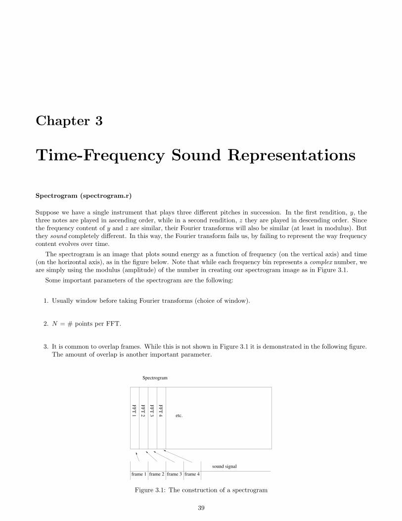
The spectrogram is an image that plots sound energy as a function of frequency (on the vertical axis) and time(on the horizontal axis), as in the figure below. Note that while each frequency bin represents a complex number, weare simply using the modulus (amplitude) of the number in creating our spectrogram image as in Figure 3.1.
Some important parameters of the spectrogram are the following:
1. Usually window before taking Fourier transforms (choice of window).
2. N = # points per FFT.
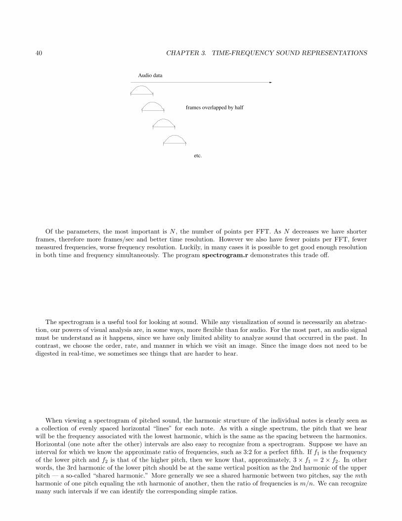
3. It is common to overlap frames. While this is not shown in Figure 3.1 it is demonstrated in the following figure.The amount of overlap is another important parameter.
FFT 1
FFT 2
FFT 3
FFT 4
frame 1 frame 2 frame 3 frame 4
Spectrogram
sound signal
etc.
Figure 3.1: The construction of a spectrogram
39
40 CHAPTER 3. TIME-FREQUENCY SOUND REPRESENTATIONS
frames overlapped by half
etc.
Audio data
Of the parameters, the most important is N , the number of points per FFT. As N decreases we have shorterframes, therefore more frames/sec and better time resolution. However we also have fewer points per FFT, fewermeasured frequencies, worse frequency resolution. Luckily, in many cases it is possible to get good enough resolutionin both time and frequency simultaneously. The program spectrogram.r demonstrates this trade off.
The spectrogram is a useful tool for looking at sound. While any visualization of sound is necessarily an abstrac-tion, our powers of visual analysis are, in some ways, more flexible than for audio. For the most part, an audio signalmust be understand as it happens, since we have only limited ability to analyze sound that occurred in the past. Incontrast, we choose the order, rate, and manner in which we visit an image. Since the image does not need to bedigested in real-time, we sometimes see things that are harder to hear.
When viewing a spectrogram of pitched sound, the harmonic structure of the individual notes is clearly seen asa collection of evenly spaced horizontal “lines” for each note. As with a single spectrum, the pitch that we hearwill be the frequency associated with the lowest harmonic, which is the same as the spacing between the harmonics.Horizontal (one note after the other) intervals are also easy to recognize from a spectrogram. Suppose we have aninterval for which we know the approximate ratio of frequencies, such as 3:2 for a perfect fifth. If f1 is the frequencyof the lower pitch and f2 is that of the higher pitch, then we know that, approximately, 3 × f1 = 2 × f2. In otherwords, the 3rd harmonic of the lower pitch should be at the same vertical position as the 2nd harmonic of the upperpitch — a so-called “shared harmonic.” More generally we see a shared harmonic between two pitches, say the mthharmonic of one pitch equaling the nth harmonic of another, then the ratio of frequencies is m/n. We can recognizemany such intervals if we can identify the corresponding simple ratios.

41
For instance, in the above figure the 2nd and 4th notes clearly have a 3:2 ratio so we see that the 2nd note is aperfect 5th higher than the 4th note. Similarly the 4th harmonic of the 3rd note is close to the 5th harmonic of the4th note, thus these notes have the frequency relationship of 5:4 and constitute a major third.
We can also recognize the traits of noisy sounds from a spectrogram in terms of high and low frequency contentand, perhaps more important, the time evolution of these traits. The spectrogram.r program can be used toexamine the variety of percussion sounds on the course web page and, perhaps, even to identify them. We willdiscuss this in detail in class.
Time-Frequency Sound Representations
The spectrogram is created by plotting just the amplitude or modulus of each time-frequency bin as brightness.While this corresponds quite naturally to much of what we hear in sound — time evolving frequency energy — thespectrogram discards the important information of the phase. In fact, there may be many time functions that wouldproduce the same, or nearly the same, spectrogram, so it is not possible to recover the time domain signal from
42 CHAPTER 3. TIME-FREQUENCY SOUND REPRESENTATIONS
a spectrogram. This is unfortunate since, though the spectrogram domain seems like an natural place to performmodifications of our sound, we have no way to convert these processed images back into sound. This can be remediedwith the time-frequency sound representation we discuss here.
The short time Fourier transform (STFT) is analogous to the spectrogram, except that we retain a complexnumber for each time-frequency bin. Thus the picture of the STFT is identical to Figure 3.1, except we do notdiscard the phase information.
Stated informally, let w(j) be our N -point window function where we regard w(j) = 0 for j 6∈ 0, . . . , N − 1.Let x0, x1, . . . be our signal. Let H be the hop size (the number of samples between STFT “frames.”) If X is theSTFT of x, we will write
xSTFT←→ X
where X = X(t, n) is given by X(t, ·) = FFT (w× tth frame of x) — that is, the tth column of X is the FFT of thewindowed tth frame of the signal.
More formally,
X(t, n) =N−1∑j=0
x(tH + j)w(j)e−2πijn
N
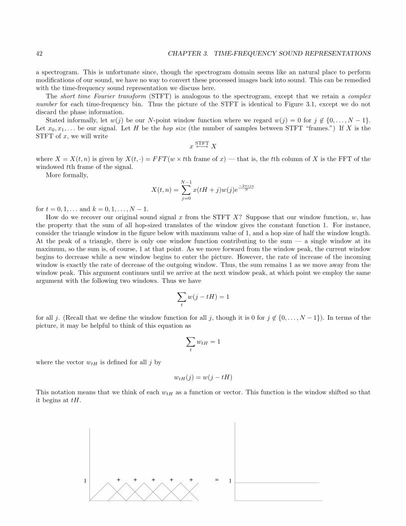
for t = 0, 1, . . . and k = 0, 1, . . . , N − 1.How do we recover our original sound signal x from the STFT X? Suppose that our window function, w, has
the property that the sum of all hop-sized translates of the window gives the constant function 1. For instance,consider the triangle window in the figure below with maximum value of 1, and a hop size of half the window length.At the peak of a triangle, there is only one window function contributing to the sum — a single window at itsmaximum, so the sum is, of course, 1 at that point. As we move forward from the window peak, the current windowbegins to decrease while a new window begins to enter the picture. However, the rate of increase of the incomingwindow is exactly the rate of decrease of the outgoing window. Thus, the sum remains 1 as we move away from thewindow peak. This argument continues until we arrive at the next window peak, at which point we employ the sameargument with the following two windows. Thus we have∑
t
w(j − tH) = 1
for all j. (Recall that we define the window function for all j, though it is 0 for j 6∈ 0, . . . , N − 1). In terms of thepicture, it may be helpful to think of this equation as∑
t
wtH = 1
where the vector wtH is defined for all j by
wtH(j) = w(j − tH)
This notation means that we think of each wtH as a function or vector. This function is the window shifted so thatit begins at tH.
11 + + + + + =
43
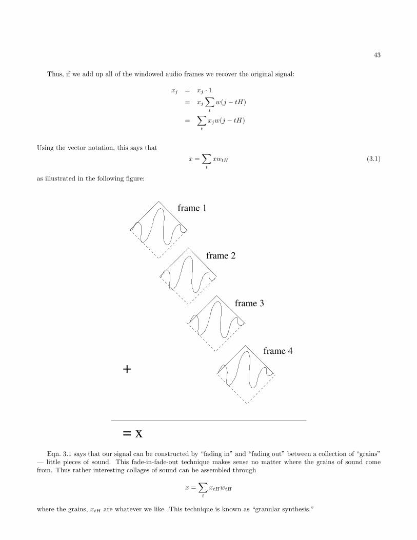
Thus, if we add up all of the windowed audio frames we recover the original signal:
xj = xj · 1
= xj∑t
w(j − tH)
=∑t
xjw(j − tH)
Using the vector notation, this says that
x =∑t
xwtH (3.1)
as illustrated in the following figure:
+
= x
frame 1
frame 2
frame 3
frame 4
Eqn. 3.1 says that our signal can be constructed by “fading in” and “fading out” between a collection of “grains”— little pieces of sound. This fade-in-fade-out technique makes sense no matter where the grains of sound comefrom. Thus rather interesting collages of sound can be assembled through
x =∑t
xtHwtH
where the grains, xtH are whatever we like. This technique is known as “granular synthesis.”
44 CHAPTER 3. TIME-FREQUENCY SOUND REPRESENTATIONS
Inverting the STFT (stft.r)
Suppose thatx
STFT←→ X
and that the STFT is constructed using the window length N , hop size H, and window function w having theproperty ∑
t
w2(j − tH) = 1
for all j. Equivalently, we could write this as ∑t
w2tH = 1
where we mean the constant vector 1 on the right. For example, consider our favorite (and only) Hann window
w(j) =
1+cos(2πj/N−π)
2√
3/2j = 0, 1, . . . , N − 1
0 otherwise
where we have added a constant of√
3/2 in the denominator. The program hanning translate.r demonstratesthat the Hann window has this property when H = N/4, though it is easy to verify by direct computation usingbasic properties of sine and cosine. By the definition of the STFT, we know that
FFT−1(X(t, ·)) = (tth frame of x)w
so thatFFT−1(X(t, ·))w = (tth frame of x)w2
From this it follows that
xj = xj∑t
w2(j − tH)
=∑t
xjw(j − tH)︸ ︷︷ ︸inverse of X(t, ·) shifted to tH
w(j − tH)
=∑t
1N
N−1∑n=0
X(t, n)e2πi(j−tH)n
N w(j − tH)
This formula simply says that, to recover x, we simply take the inverse FFT’s of each column of X, multiply theseagain by our window function, and add these up, treating the tth inverse FFT as a N -length sequence beginning attH.
Writing this in our vector notation, this reads
x =∑t
1N
(FFT−1X(t, ·))tHwtH
where, in both cases, the tH subscript means shifting by tH. Thus we simply overlap and add the shifted andwindowed inverse Fourier transforms.
This process is demonstrated in the R program stft.r. In this program we define two functions, one for the STFTand one for the inverse STFT. The program demonstrates that we can recover the original time sequence by playthe audio that is recovered using the inversion formula.
STFT Applications 1: Compression (compression.r)
The STFT gives a representation of an audio signal, x, as
xj =∑t,n
1NX(t, n)e2πin(j−tH)/Nw(j − tH)

45
through our inversion formula. Writing eiθ = cos(θ) + i sin(θ), we can express x as
x(j) =∑t,n
1N
Re(X(t, n))︸ ︷︷ ︸αtn
cos(2πn(j − tH)/N)w(j − tH)︸ ︷︷ ︸φtn(j)
+− 1N
Im(X(t, n))︸ ︷︷ ︸βtn
sin(2πn(j − tH)/N)w(j − tH)︸ ︷︷ ︸ψtn(j)
=∑t,n
αtnφtn(j) + βtnψtn(j)
Thus x is expanded in terms of the basis functions φtn, ψtn.These basis functions are simply windowed sinusoids as in the figure below, occurring at various places in
the time domain as given by t (the functions φtn and ψtn are shaped like those depicted, but are offset by tH.)
0 200 400 600 800 1000
−0.5
0.00.5
1.0
Index
cos(5
* t) * w
0 200 400 600 800 1000
−1.0
−0.5
0.00.5
1.0
Index
cos(10
* t) *
w
0 200 400 600 800 1000
−1.0
−0.5
0.00.5
1.0
Index
cos(15
* t) *
w
0 200 400 600 800 1000
−1.0
−0.5
0.00.5
1.0
Index
cos(20
* t) *
w
Such a representation has interesting applications in signal denoising. Viewed in terms of the representationabove, many of the αtn, βtn coefficients of an audio file will be negligibly small. Setting such coefficients to zerowill have the effect of denoising the signal since most of these coefficients may, in fact, be due to unwanted noise.
Similarly, the above basis representation can be used as a means for audio compression. We can approximateour signal by retaining only the largest p percent of the coefficients, and assuming the others are 0. Of course, ourcompressed audio file would need to give both the (t, n) locations we choose to retain, as well as the associatedcoefficients. The quality of the signal will degrade as p decreases to 0, but there may be usable audio representationsalong the way that require significantly less storage than the original audio representation. Both of these possibilities,denoising and compression, are demonstrated in the R program compression.r.
STFT Applications 2: Desoloing
Suppose we begin with a recording x of a soloist with accompaniment, such as a violin soloist with orchestra, or avocal soloist with rock band. Such a signal could be represented as a sum of these two parts:
x = s+ o
where x, s, o are audio vectors with s and o the solo and accompaniment parts of the “signal.” (Remember that theresult of these two sources is additive). We would like to decompose x into s and o, thus recovering an accompaniment,

46 CHAPTER 3. TIME-FREQUENCY SOUND REPRESENTATIONS
o that could be used for Karaoke or other purposes, and recovering a recording of the soloist s in isolation. How canwe do this?
An equivalent problem statement is to decompose the STFT, X, as
X(t, n) = S(t, n) +O(t, n)
where S(t, n) and O(t, n) are the solo and accompaniment STFTs. This problem (in either domain) is known asblind source separation and is quite difficult.
One possible approach is to classify each time-frequency point (t, n) as either solo or accompaniment. We couldrepresent this classification by a function
1S(t, n) =
1 if (t, n) classified as solo0 otherwise
where S is the set of (t, n) points classified as solo. We then could approximate our solo and orchestra decompositionby
S = 1SXO = 1ScX
where Sc is the complement (everything else) of S Such an approach is known as masking where 1S is the mask thatis applied to recover the solo part.
In this case it is clear that we haveX = S + O
essentially by definition. We can recover our approximations of solo and accompaniment by
sSTFT←→ S
oSTFT←→ O
Thus this approach phrases source separation as a binary classification problem where we classify each (t, n) pointas solo or accompaniment. Such an approach may work reasonably well when the majority of (t, n) are primarilythe result of either the solo or the accompaniment. Time-frequency points where both sources make significantcontributions are known as collision points. In general, it is very difficult to separate such points into their twocontributions.
An alternative to the blind (no prior knowledge) approach uses a score-match between the audio data and thesymbolic representation of the music — this is an alignment between a score and an audio file indicating where inthe audio file the various score events occur. We will discuss the problem of estimating such a correspondence laterin this class. With such a representation, we know the times of each of the solo notes, as well as the approximatefundamental frequencies for these notes, as specified in the score. Thus we know the approximate (t, n) time-frequencypoints that correspond to the solo. In performing source separation we could either work directly from the scorematch to estimate S, or try to combine both the score match and other attributes of the audio data itself to estimateS. This latter approach is demonstrated at http//:xavier.informatics.indiana.edu/˜craphael/cmj07 on bothartificially mixed, and real recordings.
The Importance of Phase (phase scramble.r, robot whisper.r)
We have claimed that some situations allow us to vary phase in our sound representation with little or no perceptualchange. Such an example is the additive synthesis model for a pitched sound
x(t) = α1 sin(2πft+ φ1) + α2 sin(2π2ft+ φ2) + . . .+ αn sin(2πnft+ φn)
=n∑k=1
αk sin(2πkft+ φk)
In this model we get no perceivable change in sound as we choose different values for the phases φk. This isdemonstrated by the phase scramble.r program, which repeatedly uses the additive synthesis model with the same

47
amplitudes, but randomly chosen phases. The same is true of the extension of this idea to a sound with time-varyingpitch, f(t):
x(t) =n∑k=1
αk sin(2πk∫ t
0
f(τ)dτ + φk).
In contrast, the choice of the phase in our STFT time-frequency representation, plays a crucial role in determiningthe nature of the corresponding sound. One very simple example is when we take an STFT of actual sound, set allthe phases to 0, and invert the STFT. That is
xSTFT←→ X
X(t, n) = |X(t, n)|+ 0i
xSTFT←→ X
The original and resulting audio can be heard through the program robot whisper.r. While the original audiomay have a variety of time-varying pitch content, the “roboticized” audio comes across at a single pitch. This issomething like the difference between regular speech and monotone speech. Why does this happen?
Let us first suppose that our sound is pitched (perhaps with several pitches) and completely steady state, notchanging in pitch, amplitude, or timbre. In this case the spectrogram of the sound would appear as a collection ofcompletely straight horizontal lines corresponding to the frequencies present in the signal. Since the frequency contentis constant over our frames, and we have set all phases to 0, the “columns” of our STFT, X(t, ·), for t = 0, 1, . . . areidentical. Suppose we let
v = w · FFT−1X(t, ·)
be the inverse FFT of one of these columns (they are all the same), multiplied by our window function.Our STFT inversion algorithm tells us we must reconstruct the time signal by adding together shifted copies of
v:x =
∑t
vtH
where, as usual, vtH(j) = v(j − tH). Suppose, to be definite, H = N/4 and let v1, v2, v3, v4 be the frame v dividedinto 4 equal pieces of length H. Now when we overlap add, the process looks as depicted below:
. . . . . .v v v v
v vv v
v vv v
v
vvvv
v
1
11
1
11
22
22
2
33
33
44
4
v v vvv
v
2 33
44
4
+v v v v v v+ + + + + +
H
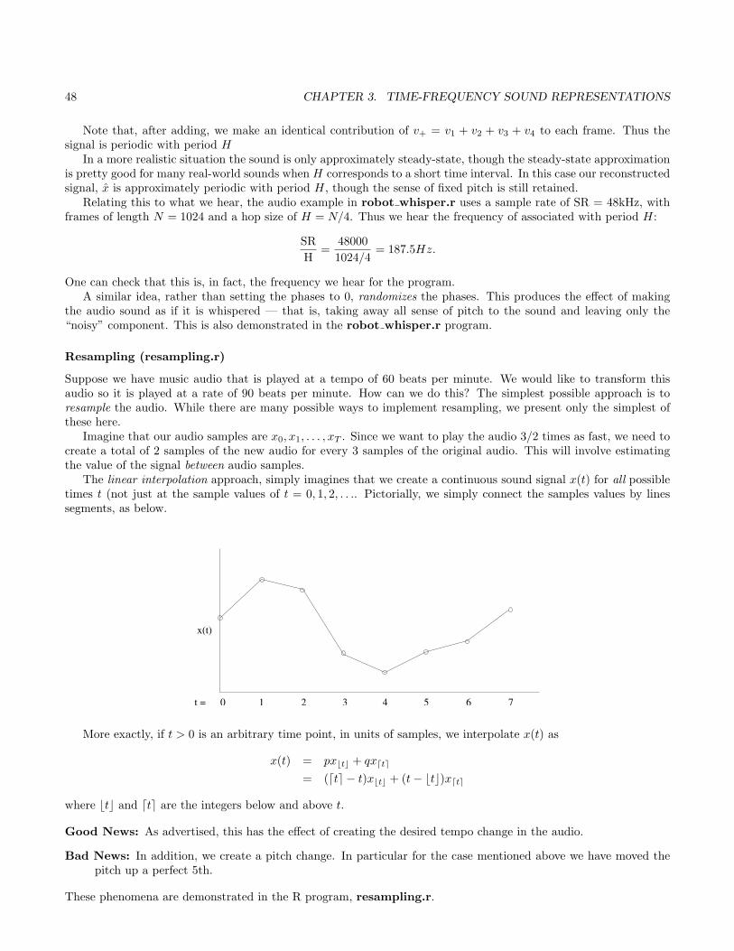
48 CHAPTER 3. TIME-FREQUENCY SOUND REPRESENTATIONS
Note that, after adding, we make an identical contribution of v+ = v1 + v2 + v3 + v4 to each frame. Thus thesignal is periodic with period H
In a more realistic situation the sound is only approximately steady-state, though the steady-state approximationis pretty good for many real-world sounds when H corresponds to a short time interval. In this case our reconstructedsignal, x is approximately periodic with period H, though the sense of fixed pitch is still retained.
Relating this to what we hear, the audio example in robot whisper.r uses a sample rate of SR = 48kHz, withframes of length N = 1024 and a hop size of H = N/4. Thus we hear the frequency of associated with period H:
SRH
=480001024/4
= 187.5Hz.
One can check that this is, in fact, the frequency we hear for the program.A similar idea, rather than setting the phases to 0, randomizes the phases. This produces the effect of making
the audio sound as if it is whispered — that is, taking away all sense of pitch to the sound and leaving only the“noisy” component. This is also demonstrated in the robot whisper.r program.
Resampling (resampling.r)
Suppose we have music audio that is played at a tempo of 60 beats per minute. We would like to transform thisaudio so it is played at a rate of 90 beats per minute. How can we do this? The simplest possible approach is toresample the audio. While there are many possible ways to implement resampling, we present only the simplest ofthese here.
Imagine that our audio samples are x0, x1, . . . , xT . Since we want to play the audio 3/2 times as fast, we need tocreate a total of 2 samples of the new audio for every 3 samples of the original audio. This will involve estimatingthe value of the signal between audio samples.
The linear interpolation approach, simply imagines that we create a continuous sound signal x(t) for all possibletimes t (not just at the sample values of t = 0, 1, 2, . . .. Pictorially, we simply connect the samples values by linessegments, as below.
72 3 4 5 61
x(t)
0t =
More exactly, if t > 0 is an arbitrary time point, in units of samples, we interpolate x(t) as
x(t) = pxbtc + qxdte
= (dte − t)xbtc + (t− btc)xdte
where btc and dte are the integers below and above t.
Good News: As advertised, this has the effect of creating the desired tempo change in the audio.
Bad News: In addition, we create a pitch change. In particular for the case mentioned above we have moved thepitch up a perfect 5th.
These phenomena are demonstrated in the R program, resampling.r.

49
We see now that what seemed to be a simple notion — just changing the tempo of the audio — becomes somewhatmurky from a scientific perspective. That is, we are trying to change the rate of the audio at the note level (tempo),while not changing the rate of audio at the period level (pitch). Thus the goal of audio time-stretching is perceptuallyclear, but not well-posed from a scientific standpoint. We will proceed bravely, without having clearly articulatedour goal.
The Shannon Sampling Theorem
This section on the Shannon theorem constitutes a brief digression from the main thrust of our course. This theoremis one of the main results of any serious introductory class to signal processing, and it is too good to completely leaveout. Though it might not have many direct applications for our purposes, other than resampling, it is a gem that isworth knowing.
Linear interpolation allows us to take a sequence x0, x1, . . . and to produce a function x(t) that “agrees” withthe sampled values, yet gives a value for all t. While linear interpolation methods may work reasonably well for avariety of situations, such as small changes of playback rate and pitch, such techniques can function quite poorly inother cases, such as resampling to lower sampling rate. A surprising fact is that there is a “correct” way to recoverthe continuous-time signal, x(t), from its samples, known as the Shannon Sampling Theorem.
The hypothesis of the Shannon Theorem deals with a time signal, x(t), before it has been sampled. Recall thatif we have a sampling rate of SR, then the highest frequency we can represent is the so-called Nyquist frequency,SR/2. The Shannon theorem assumes that the original signal, x(t), has no frequency content above SR/2. If it did,we know the sampling procedure would produce aliasing. Assuming this criterion is met, we can recover the originalsignal, x(t), exactly only knowing the samples . . . , x−2, x−1, x0, x1, x2, . . .. This is done according to the formula
x(t) =∞∑
j=−∞xjφ(t− j) (3.2)
where φ(t) is known as the sinc function, and defined by
φ(t) =sin(πt)πt
Though it may not be clear from the definition, the right way to define φ(0) is by φ(0) = limt→0 φ(t) = 1. The sincfunction is shown in the figure below:
−5 0 5
−0.20.0
0.20.4
0.60.8
1.0
t
f
−7 −6 −5 −4 −3 −2 −1 0 1 2 3 4 5 6 7
Note that φ(t) is 1 at 0 and is 0 at all of the other integral values of t, thus using Eqn. 3.2 for integral j′ we mustget
x(j′) =∞∑
j=−∞xjφ(j′ − j) = xj′
That is, x(t) is consistent with the sampled values, which is comforting. Pictorially, Eqn. 3.2 says that we reconstructthe original function x(t) by adding up scaled sinc functions at the sample locations, where we use the sample valuesas the scaling constants, as shown below.

50 CHAPTER 3. TIME-FREQUENCY SOUND REPRESENTATIONS
−5 0 5
−10
12
34
5
t
f1
−5 0 5
−10
12
34
5
t
f1 + f2 +
f3
The upper figure shows the situation in which all of our samples are 0 except for the ones collected at 0, 1 and2, where we have the sample values 5,4, and 3. We reconstruct by putting a sinc function at the locations 0,1 and 2,scaled by the sample values, as shown in the top panel of the figure. Our reconstruction is the sum of these functions,shown in the bottom panel.
The Shannon theorem gives a more principled alternative to resampling by linear interpolation. Linear interpo-lation makes the unrealistic assumption that the our time function continues linearly between sample values. TheShannon theorem tells us exactly how the unseen parts of the function behave, only by considering the sampledvalues. Better results can be achieved by using (or approximating) the continuous time values given by the Shannontheorem when resampling.
Phase Vocoder (phase vocoder.r)
Consider the following experiment in which we try to make continuous sound out of a single FFT spectrum. To dothis, we take our FFT and replicate it over and over to produce our STFT. We then use the usual inversion formulato construct the actual sound. This experiment is demonstrated in the R program phase vocoder motivation.r.Clearly it doesn’t work, though it would be a good idea to try to understand why.
It is easiest to visualize the problem when our sound consists of a single sine wave, though not necessarily one ofthe FFT analysis frequencies. In particular, we assume that our sine wave is not periodic over H samples. In thiscase our reconstruction of the signal will be the sum of the windowed sinusoid, overlapped as in the picture below.

51
ba
To understand the effect of the situation we make a brief digression. Suppose we have a sum of two sine waveseach of the same frequency, but with different amplitudes and phases:
x(t) = a1 sin(2πft+ φ1) + a2 sin(2πft+ φ2)
It is well-known that the result is also a sine wave of frequency f , with an amplitude and phase having a simplerelation to the a1, a2, φ1, φ2. The result can be visualized using the “parallelogram” rule. That is, if we add thevector with length a1 and angle φ1 to the vector with length a2 and phase φ2, we get a new vector whose length andangle are the amplitude and phase of the resulting sine wave. This is demonstrated in the picture below.
a
a
1
2
φ
φ
φ
2
1
a
From the picture we see that when we add two sine waves that have identical phases, then the amplitudes add.Otherwise there is some degree of cancellation between the sines and the resulting amplitude will be less than the

52 CHAPTER 3. TIME-FREQUENCY SOUND REPRESENTATIONS
sum of the amplitudes.In terms of our original picture, consider the two time points a and b, indicated by the vertical lines. At a our
overlap and add only involves a single sine wave, since we are at the center of the window and H = N/2. Thus inthe neighborhood of a we would see a sine wave of the original amplitude. At the point b we are adding together twosine waves each scaled by 1/2 due to the Hann window. Since our signal is not H-periodic, the two sines will havedifferent phase. Thus, when we combine them at point b there will be some cancellation, resulting in a decrease inthe resulting amplitude. Of course, the amount of interference we vary smoothly as we move between a and b.
If we look at the result from a more global perspective, we will see the resulting overlap add process oscillatingbetween higher and lower resulting amplitudes as we move through the regions of various degrees of cancellation.The result will be a sine wave whose amplitude varies periodically with period given by the hop size H, as in thepicture below. Clearly this is not what we want.
0 500 1000 1500 2000 2500
−1.0−0.5
0.00.5
1.0
Index
s * u
This is the picture of what we heard in the audio produced by phase vocoder motivation.r. Luckily, there isa simple way to fix this problem, as follows.
Suppose we compute the STFT for our original (non H-periodic) sinusoidal signal, x(t). There is, of course,nothing interesting happening as far as the amplitude of the individuals FFTs are concerned, each showing a peakaround the relevant frequency, f . However, we will see a different phase in each of the frames, as indicated below.
Phase
Moreover, since our frequency is constant, the difference in phase between adjacent frames will also be a constant.We’ll call this phase difference ∆φ, measured in radians. Thus, if we wanted to avoid cancellation when our overlappedframes are added, we would offset each successive frame by ∆φ over the previous frame. Thus, for our single sinusoid,the frames would be
x0(t) = w(t) sin(2πft)x1(t) = w(t− 1H) sin(2πft+ ∆φ− 1H)x2(t) = w(t− 2H) sin(2πft+ 2∆φ− 2H)x3(t) = w(t− 3H) sin(2πft+ 3∆φ− 3H)
......

53
The idea of the phase vocoder is to use this same argument for each of the FFT frequencies, and for eachwindowed “grain” of sound. For the phase vocoder, we take a “snapshot” of sound for each overlapped frame as anFFT. However, rather than saving the actual phase for each analysis frequency, we save the difference in phase. Weretain the original modulus for each FFT, exactly as before. Said more precisely, if
xSTFT←→ X
defined as before, we construct the modified STFT, X, by
X(t, n) = |X(t, n)|ei∆φ(t,n)
where
∆φ(t, n) =
Arg(X(t, n)) if t = 0Arg(X(t, n))−Arg(X(t− 1, n)) otherwise
That is, for each row of the STFT we construct our modified STFT simply by substituting phase differences foractual phase.
It is a simple matter to invert X. All we need to do is to convert the modified STFT, X, to the regular STFT,X, by undoing the differencing. That is, if φ0, φ1, φ2, . . . are the sequence of phases we encounter on a particular rowof the X, then the corresponding row of X will have φ0, φ1 − φ0, φ2 − φ1, φ3 − φ2, . . .. We reconstruct the originalphase simply by “integrating” (performing the cumsum) on this sequence. This gives
φ0 = φ0
φ1 = φ0 + (φ1 − φ0)φ2 = φ0 + (φ1 − φ0) + (φ2 − φ1)φ3 = φ0 + (φ1 − φ0) + (φ2 − φ1) + (φ3 − φ2)
......
Using this idea we rewrite our STFT routine to compute the modified STFT, X, instead of the straight STFT,X. To recover audio from X, we simply need to perform cumsum on each of the rows of X and then continuewith the regular STFT inversion. This modified STFT and its inverse are given as functions in the R programphase vocoder.r.
Why would we want to add this extra and, perhaps, seemingly pointless step to our definition of the STFT?Returning to our original goal of creating audio by replicating a single frame over and over, suppose we replicateover and over the first column of X rather than the first column of X. Once we do this we no longer have problemwith changing amounts of cancellation between our audio frames during the inversion process. More generally, themodified view of the STFT guarantees that, for each analysis frequency, each new frame continues the phase fromwhere the previous frame left off. Thus, we can now construct an STFT by piecing together STFT frames in anymanner we like.
Phase Vocoder Examples
The program phase vocoder.r shows two simple examples in which we perform:
time stretching by either replicating or deleting some of the STFT frames
random assembly since the phase vocoder is designed to create phase discontinuity, even randomizing the orderof STFT frames will produce continuous sounding audio.
In addition we will do two examples in class that are not computed in R, and do not have corresponding programson the class website. The first of these shows a real-time implementation of phase vocoding that allows a personto play through an audio file, continually changing the play rate. When the play rate is 1, we get the originalaudio, nearly exactly as it was, courtesy of the STFT inversion formula. As the rate changes, we assemble frames bycalculating our current position, in frames, according to the play rate. For instance, if the play rate is .5, we wouldadvance 1/2 a frame for each output frame. That is, we would repeat each frame twice. Using this idea it is possibleto move through the audio at any rate, including 0 (stalling the sound at a particular point), or a negative rate

54 CHAPTER 3. TIME-FREQUENCY SOUND REPRESENTATIONS
(moving backwards through the audio file). It is interesting to note that, while we retain phase continuity throughour phase vocoding procedure, we introduce other undesirable elements into the sound. For instance as we slowdown the playback rate, we also slow down the reverberation decay of the room, the attack time, the vibrato rate,and other musical attributes that normally do not depend on tempo. These can produce unrealistic sounding audio,though are often not noticeable at play rate near 1.
A second example we will show in class is called the “Oracle.” With the Oracle, we take a recording of a soloinstrument playing in isolation. Using score following, as will be discussed, we can approximate the audio positionsof all of the notes in the soloist’s score. We will do the same for a recording of the orchestral accompaniment tothe soloist. Even though these two performances were made with no knowledge whatsoever of each other, we canuse phase vocoding to match the timing of the orchestra performance to to soloist, thereby generating an orchestralaccompaniment after the fact.
To do this, suppose that k indexes the score positions at which we have have coincident notes between the soloand orchestra parts. From our score match, we can compute the solo times for these events, s1, s2, . . ., as well asthe orchestra times for the events, o1, o2, . . .. Note that these sequences only contain the musical positions havingcoincident solo and orchestra notes. In the figure below we have plotted the points (sk, ok) and interpolated betweenthem to produce the function u(t).
s s s s
o
o
oo1
2
3
4
1 2 3 4t
u(t)
If we measure the sk and ok in units of the STFT hop size, H, then the function u(t) in the figure showshow we need to warp the orchestra recording to match the accompaniment. Specifically, we will create our warpedversion of the orchestra, X, by
X(t, n) = X(u(t), n)
where X is the straight STFT of the orchestra performance. If u(t) is not an integer for some t, we just round it tothe nearest integer and take the corresponding frame of the orchestra STFT. We will get our accompaniment audioby taking the inverse STFT of X. We will demonstrate several examples of this procedure in class.

Chapter 4
Recognition of Audio and Applications
Score Alignment
The problem of score alignment seeks a correspondence between a musical score and an audio performance of thatscore. For this problem we assume that the musical score is represented in a symbolic format, giving, say, the MIDIpitches of the score and the corresponding onset times, in beats or some other unit of musical time. The scoremay have an approximate tempo, but we assume the performer has considerable latitude in playing the music. Forinstance, a simple score format representing “Mary had a Little Lamb” format may look like the following, wherewe have used whole notes as the unit of musical time. This is often a reasonable unit to use since a quarter (or half,eighth, sixteenth, etc.), is one quarter (or half, eighth, sixteenth) of a whole note, regardless of the meter.
onset MIDI0/4 641/4 622/4 603/4 624/4 645/4 646/4 648/4 629/4 6210/4 62
Our score alignment could be thought of as a third column to this table giving the onset time of the notes intime units such as seconds. This score match is depicted in the figure below.
audio data
55

56 CHAPTER 4. RECOGNITION OF AUDIO AND APPLICATIONS
There are two different kinds of score alignment problems, having different kinds of applications: Offline alignmentworks using the complete audio file. Thus the algorithm can consider both past and future music data in trying todetermine the onset time of a particular note. On the other hand, online alignment, also known as score following,processes the audio data as it comes in, with no potential to consider future music data. This is the appropriatetechnique when some real-time response to the incoming audio is desired.
What follows is a brief list of possible applications of these problems, though there are many possible additions.
Offline Alignment
Random Audio Access This allows one to hear or see the audio at any position in the music, specified in musicalunits. Think of all the times you have searched for a particular place in a piece of music.
Editing Digital Audio The usual process of making an audio recording may involve some splicing together ofvarious performances or fixing isolated problems individual tracks. A score alignment allows one to easilyidentify the section of audio corresponding to a particular note or event for further processing.
Coordination of Media Sometimes we may want to align music with some other possible medium, such as videoor more audio. The “Oracle” was an example of aligning two different audio performances, in that case a soloand orchestra. For instance, we may want to create an animated dance video that synchronizes to prerecordedmusic. The score alignment gives the precise times at which the various video events must occur. Anotherexample would be warping video of a conductor to follow a performance.
Quantitative Description of Performance We may want to give a performer or musicologist precise feedbackregarding the tuning, timing, or some other aspect of performance. For instance, there has been a good deal ofinterest in studying timing and the way it relates to musical expression. Another example is a tuning system,designed to show a musician places where tuning inaccuracies occur in the context of a musical score.
Database Collections Sampled sound is now a fundamental element of many (perhaps most) synthetic instru-ments. Generally, sampled audio is obtained by having a musician play a collection of notes in a highlycontrolled environment — typically such data is in short supply. Score alignment could be used to mine largequantities of sample data from preexisting recordings.
Online Alignment (Score Following)
Musical Accompaniment Systems These are programs that provide flexible live accompaniment to a musicianthat synthesizes the missing parts. More on this in what follows.
Content-Based Audio Processing Programs such as Autotune have been highly successful in recent years incorrecting the tuning in a performance. Live implementations are possible, but made difficult by the uncertaintyof knowing the actual note the performer is aiming for. Score following makes the note identifications muchsimpler.
New Music Applications Similar in spirit to the above, but different in the kinds of applications, one may wishto apply audio effects in a selective score-dependent way. For instance one could harmonize, distort, modify asequence of notes differently, in real time. This can prove a powerful tool for new music.
Supertitles or other media such as lights can be coordinated with live performance automatically.
Automatic Page Turners could make the keyboard player’s life much easier by turning pages as required.
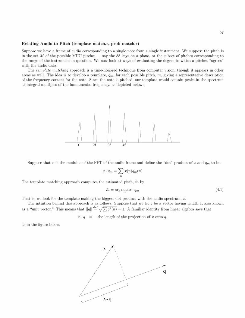
57
Relating Audio to Pitch (template match.r, prob match.r)
Suppose we have a frame of audio corresponding to a single note from a single instrument. We suppose the pitch isin the set M of the possible MIDI pitches — say the 88 keys on a piano, or the subset of pitches corresponding tothe range of the instrument in question. We now look at ways of evaluating the degree to which a pitches “agrees”with the audio data.
The template matching approach is a time-honored technique from computer vision, though it appears in otherareas as well. The idea is to develop a template, qm, for each possible pitch, m, giving a representative descriptionof the frequency content for the note. Since the note is pitched, our template would contain peaks in the spectrumat integral multiples of the fundamental frequency, as depicted below:
2ff 3f 4f
Suppose that x is the modulus of the FFT of the audio frame and define the “dot” product of x and qm to be
x · qm =∑n
x(n)qm(n)
The template matching approach computes the estimated pitch, m by
m = arg maxm
x · qm (4.1)
That is, we look for the template making the biggest dot product with the audio spectrum, x.The intuition behind this approach is as follows. Suppose that we let q be a vector having length 1, also known
as a “unit vector.” This means that ||q|| def=√∑
q2(n) = 1. A familiar identity from linear algebra says that
x · q = the length of the projection of x onto q.
as in the figure below:
x q
q
x
.

58 CHAPTER 4. RECOGNITION OF AUDIO AND APPLICATIONS
As can be seen from the figure, the dot product gets larger as the vectors “point” in similar directions. Thus ifwe scale all of our templates to have unit length (q′m = qm
||qm|| ), then choosing the best template match from Eqn. 4.1is the same as looking for the template qm that points most nearly in the same direction as x. For this argument tomake sense, we must normalize our templates to all have length 1 before using the template match procedure. Thisapproach is demonstrated in the R program template match.r.
A variant on this approach is described by the following simple probabilistic model, though first we introduce alittle background in probability.
Suppose we have an experiment that can occur in N ways, 1, 2, . . . , N. Let p1, p2, . . . , pN be the probabilitiesof these outcomes having
1. pn ≥ 0
2.∑n pn = 1
Suppose we observe a sequence of J independent trials of the experiment with outcomes x1, x2, . . . , xJ , say x1 =3, x2 = 5, x3 = 4 . . .. The probability of this particular sequence is then
P (x1, . . . , xJ) = px1px2 . . . , pxJ= p#1′s
1 p#2′s2 . . . p#N′s
N
Now we view our actual spectrum x as a histogram, so that x contains x(1) observations of frequency 1, x(2)observations of frequency 2, etc. We also view our template qm (scaled to sum to 1) as a probability distribution, sothat if pitch m is sounding, x is regarded as a random sample from qm. Thus the probability of observing x when mis sounding is
P (x|qm) = qm(1)x(1)qm(2)x(2) . . . qm(N)x(N)
With this probabilistic model, the maximum likelihood strategy is to choose the model, qm giving the greatestlikelihood to the data. That is
m = arg maxm
P (x|qm)
= arg maxm
N∏n=1
qm(n)x(n)
= arg maxm
N∑n=1
x(n) log qm(n)
= arg maxm
x · log qm
Observe that this is very much like our template matching approach except we take the dot product with the logof our template, rather than the template itself. This approach is demonstrated in the R program prob match.r.The probabilistic approach has the advantage that we can choose our templates qm in a principled way: If we believedthe assumptions of the model, a natural estimate for qm would be just the average of a number of spectra that weregenerated by pitch m.
Dynamic Programming
A graph is a construction from computer science and discrete mathematics composed of a collection of nodes andedges. The nodes are places we might visit in the graph, while we can only travel between nodes that are connectedby edges. A particular kind of graph is called a trellis — while more general definitions are possible, we call a grapha trellis if each of the nodes lives at a level: 0, 1, 2, . . . , n and all edges connect nodes at successive levels. Such atrellis graph is depicted below.

59
12
7
5
6
3
209
5432
10751
58
The graph in the figure is known as a weighted graph since each of the edges has an associated cost. A commonproblem one considers with such a graph is to find the minimal cost path from the start (leftmost node) to the end(rightmost node), where the cost of the path is the sum of the arc costs traversed along the path. This optimalpath is computed using a technique known as dynamic programming, which relies on a single simple, yet powerful,observation as follows:
For each node, n, in the trellis, the best scoring path to the node is a best scoring path to a node,m, at the previous level, plus the arc (m,n).
This is clearly true since if we were to consider a suboptimal path from the start to m plus the arc (m,n), clearlythis achieves a worse score than the optimal path to m plus (m,n). This idea is illustrated in the following figurewhere the optimal path to a node a level n is seen to be an extension of an optimal path to a node an level n:
opt path
opt path
opt path
start
n n+1
The observation leads directly to an algorithm for computing the optimal path. Let c(i, j) be the cost realized ingoing from node i to node j. Let m(i) be the cost of the optimal path from the start to node i and set m(start) = 0.Then, reasoning from our “key observation,” we see that the score of the optimal path to node j must be the best ofthe optimal paths to the predecessors, i, of j with (i, j) concatenated onto these optimal paths. Put algorithmically,we can compute the score of the optimal path from start to end by letting
m(j) = mini∈pred(j)
m(i) + c(i, j)

60 CHAPTER 4. RECOGNITION OF AUDIO AND APPLICATIONS
where pred(j) is the predecessors of j — the collection of notes that are connected to j “from the left.” We willcompute the costs m(j) from left to right in our graph. Then, when these optimal costs are all computed, m(end)will be the optimal cost from start to end.
Of course, we really wanted to find the optimal path, not just its cost. A simple addition to our algorithm solvesthis problem. Let
a(j) = arg mini∈pred(j)
m(i) + c(i, j)
so that a(j) is the optimal predecessor of node j. When we have computed a(j) and m(j) for all trellis nodes, wecan then “trace back” the optimal path by following the optimal predecessors back from the end node. That is, theoptimal path (in reverse order) is given by:
end, a(end), a(a(end)), a(a(a(end))), . . . , start
In the following simple example we have filled in the circles of each node j with the optimal cost to j, m(j), andhave indicated the optimal predecessors of each node with an arrow that points backward along the appropriate arc.
3
4
1
2
36
561
32
43
571
37
4
1
2 7
1
4
4
3 6
7
8
7
One last comment. We have presented DP as a tool for finding the minimal cost path through a trellis graph.However, if each arc has some sort of “score” attached to to, and we wish to find the highest scoring path, we simplyreplace minima by maxima in the expressions for a(j) and m(j).
Dynamic Programming Approach to Score Following
Suppose we have a score made out of three notes: C,E,G. We will ignore the rhythm associated with the notes andconsider the 5-state graph as follows:
start C E G end
We think of this graph as describing the possible sequences of frame labellings we are willing to consider. Notethat every sequence that this graph can generate looks like
start, . . . , start, C, . . . , C,E, . . . , E,G, . . . , G, end, . . . , end
This same graph can also be represented as a trellis graph where the tth layer of the trellis corresponds to the possiblelabellings of the tth audio frame. This graph is shown in the figure below.

61
Frame 1 Frame 2 Frame 3
start
C
E
G
end
If we label the rows of the trellis as start, C,E,G, end, as indicated in the figure, then the paths through ourtrellis graph create the same sequences of frame labellings is in our original 5-state graph. This is the crux of thematter and why the approach we are presenting is so far superior to the frame-by-frame labeling approach we firstintroduced: The trellis graph constrains the possible sequences of frame labels to be meaningful sequences for scorealignment.
We now want to cast our score matching problem as a search for the optimal path through our trellis graph, andto do this we must assign scores to the arcs of the trellis. To do this, the score we will give an arc that terminatesin a node in row r at column t will be
logP (X(t, ·)|model r)
where model 2,3,4 are the C,E,G models while models 1,5 is a rest model. (In this latter case of a rest we may modelthe spectrum as a sample from a uniform distribution in which all frequencies are equally likely.)
Now we can find the most likely path through this graph using dynamic programming, as discussed before. Ifl1, l2, . . . , lT is a labeling of the entire collection of T frames, then we are looking for the best scoring labeling ofsequences from the 5-state model, where the score of a labeling is
T∑t=1
logP (X(t, ·)|lt)
Implementation
This idea can be implemented with a pair of 5 × T arrays, one we will call the Score array and the other the Predarray. For these arrays
Score[j,t ] is the score of the optimal path through the trellis ending in state j at frame t.
Pred[j,t ] is index (in 1 . . . , 5) of the optimal predecessor of state (j, t).
In terms of our previous discussion, Score[j,t] is the number we wrote inside the circle representing a trellis node,while Pred[j,t] is the arrow that pointed backward to the previous optimal state.
Since this algorithm is especially important to us, we present here the R code needed to compute both the Scoreand Pred arrays. We begin by initializing the 1st column of the Score array so that
Score[j, 1] =
0 if j = 1−∞ otherwise
meaning that we force the path to begin in the start state. Then the following algorithm would fill in the remainingcolumns of the array in succession:
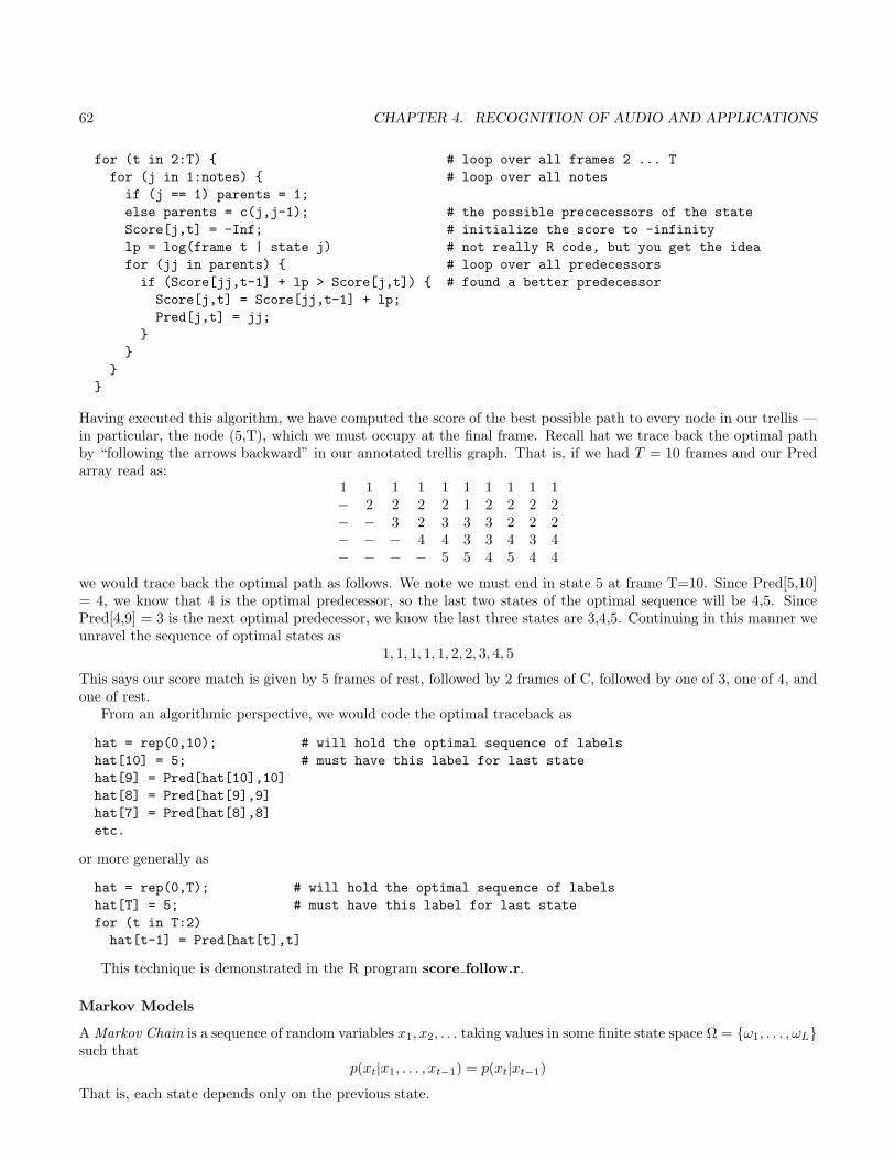
62 CHAPTER 4. RECOGNITION OF AUDIO AND APPLICATIONS
for (t in 2:T) # loop over all frames 2 ... Tfor (j in 1:notes) # loop over all notesif (j == 1) parents = 1;else parents = c(j,j-1); # the possible prececessors of the stateScore[j,t] = -Inf; # initialize the score to -infinitylp = log(frame t | state j) # not really R code, but you get the ideafor (jj in parents) # loop over all predecessorsif (Score[jj,t-1] + lp > Score[j,t]) # found a better predecessorScore[j,t] = Score[jj,t-1] + lp;Pred[j,t] = jj;
Having executed this algorithm, we have computed the score of the best possible path to every node in our trellis —in particular, the node (5,T), which we must occupy at the final frame. Recall hat we trace back the optimal pathby “following the arrows backward” in our annotated trellis graph. That is, if we had T = 10 frames and our Predarray read as:
1 1 1 1 1 1 1 1 1 1− 2 2 2 2 1 2 2 2 2− − 3 2 3 3 3 2 2 2− − − 4 4 3 3 4 3 4− − − − 5 5 4 5 4 4
we would trace back the optimal path as follows. We note we must end in state 5 at frame T=10. Since Pred[5,10]= 4, we know that 4 is the optimal predecessor, so the last two states of the optimal sequence will be 4,5. SincePred[4,9] = 3 is the next optimal predecessor, we know the last three states are 3,4,5. Continuing in this manner weunravel the sequence of optimal states as
1, 1, 1, 1, 1, 2, 2, 3, 4, 5
This says our score match is given by 5 frames of rest, followed by 2 frames of C, followed by one of 3, one of 4, andone of rest.
From an algorithmic perspective, we would code the optimal traceback as
hat = rep(0,10); # will hold the optimal sequence of labelshat[10] = 5; # must have this label for last statehat[9] = Pred[hat[10],10]hat[8] = Pred[hat[9],9]hat[7] = Pred[hat[8],8]etc.
or more generally as
hat = rep(0,T); # will hold the optimal sequence of labelshat[T] = 5; # must have this label for last statefor (t in T:2)hat[t-1] = Pred[hat[t],t]
This technique is demonstrated in the R program score follow.r.
Markov Models
A Markov Chain is a sequence of random variables x1, x2, . . . taking values in some finite state space Ω = ω1, . . . , ωLsuch that
p(xt|x1, . . . , xt−1) = p(xt|xt−1)
That is, each state depends only on the previous state.

63
Often a Markov chain is depicted with a state graph showing the states as nodes in a graph with directed(with arrow) edges showing transition probabilities. The sum of the probabilities of all edges leaving a statemust be 1. If we denote sun by S and rain by R, a sequence generated by this Markov chain would look likeSSSSSRRRRRRRRRRRSSSSSSSRRRR
rain sun
.1
.1
.9 .9
To make our definition more clear, consider the case of four random variables x1, x2, x3, x4. No matter what kindof dependence these variables have, it is always true that
p(x1, x2, x3, x4) = p(x1)p(x2|x1)p(x3|x1, x2)p(x4|x1, x2, x3)
In the case of a Markov Chain, these factors simply to:
p(x1, x2, x3, x4) = p(x1)p(x2|x1)p(x3|x2)p(x4|x3)
More generally, if x1, x2, . . . , xN is a Markov chain, then
p(x1, . . . , xT ) = p(x1)p(x2|x1)p(x3|x2) . . . p(xT |xT−1)
= p(x1)T∏t=2
p(xt|xt−1)
As a result of this, we see that in order to define a Markov chain we need
1. The initial distribution p(x1)
2. The transition probability matrix Q where Qij = p(xn+1 = ωj |xn = ωi)
For instance, in the “Rain and Sun” Markov chain introduced above, we would have two states Ω = ω1, ω2 =Rain,Sun where
Q =(Q11 Q12
Q21 Q22
)=
(p(ω1|ω1) p(ω2|ω1)p(ω1|ω2) p(ω2|ω2)
)=
(.9 .1.1 .9
)
Hidden Markov Models
Suppose we have a Markov chain, x = x1, x2, x3, . . ., but do not observe x directly. Instead, each time we visit astate, the state “outputs” a random observation from some distribution associated with the state.
As an example, consider the following figure that describes an observed sequence of coin flips. In this examplethere are two coins, a “fair” coin, F, and an “biased coin, B. The fair coin gives equal probability to H (heads) andT (tails), but the biased coin gives probability .8 to H (and .2 to T). The coin flipper flips the current coin and thenmakes a random choice of which coin to use next. In doing this, she stays with the current coin with probability .9and switches to the other coin with probability .1.

64 CHAPTER 4. RECOGNITION OF AUDIO AND APPLICATIONS
.9.9
.1
.1
H T TH
.5 .5 .2.8
BF
An observed sequence from the coin may looking something like the following.
THHTHHTTHHTT︸ ︷︷ ︸fair?
HHHTHHTHHHHHHH︸ ︷︷ ︸biased?
THTHHTH . . .︸ ︷︷ ︸fair?
In hidden Markov model problems (HMMs), the inference problem is usually to give meaning to the observations byuncovering the sequence of hidden states. This meaning (here which coin is operating) is annotated in the equationabove for the particular sequence of flips.
More formally, we assume that each observation, yn, depends only on the current state, xn. We will write x andy for the entire sequences of states and observables: x = (x1, x2, . . . , xT ), y = (y1, y2, . . . , yT ). Thus
p(y|x) = p(y1, . . . , yT |x1, . . . , xT )= p(y1|x1, . . . , xT )p(y2|y1, x1, . . . , xT ) . . . p(yT |y1, . . . , yT−1, x1, . . . , xT )= p(y1|x1)p(y2|x2) . . . p(yT |xT )
Putting this together with the factorization of the Markov chain, x, gives
p(x, y) = p(x)p(y|x)= p(x1)p(x2|x1)p(x3|x2) . . . p(xT |xT−1)×p(y1|x1)p(y2|x2)p(y3|x3) . . . p(yT |xT )
= p(x1)p(y1|x1)︸ ︷︷ ︸f(x1)
p(x2|x1)p(y2|x2)︸ ︷︷ ︸f(x1,x2)
p(x3|x2)p(y3|x3)︸ ︷︷ ︸f(x2,x3)
. . . p(xT |xT−1)p(yT |xT )︸ ︷︷ ︸f(xT−1,xT )
Usually in an HMM the y’s are observed and hence are known to us. On the other hand, the x’s are unobserved,and hence unknown. Thus, we can think of this factorization as a product of functions where the first, f(x1), justdepends on the first state variable, the 2nd, f(x1, x2), depends on the first two state variables, the third, f(x2, x3),depends on the next two state variables, etc. This view of the factorization will be important to us in what follows.
HMMs for Recognition (coin hmm.r)
Suppose we have an HMM, (x, y), with p(x, y) as before. We observe y = (y1, y2, . . . , yT ) and want to find the mostlikely state sequence given our observations. That is, we seek x = (x1, x2, . . . , xT ) where
x = arg maxx
p(x|y)
Note that since p(x|y) = p(x,y)p(y) and y is fixed, we have
x = arg maxx
p(x|y)
= arg maxx
p(x, y)
= arg maxx1,...,xT
[p(x1)p(y1|x1)]︸ ︷︷ ︸f(x1)
[p(x2|x1)p(y2|x2)]︸ ︷︷ ︸f(x1,x2)
. . . [p(xT |xT−1)p(yT |xT )]︸ ︷︷ ︸f(xT−1,xT )
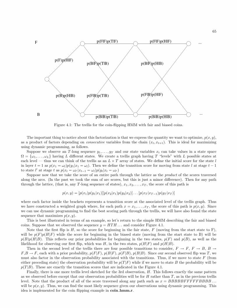
65
p(B)p(H|B)
p(F)p(H|F)
p(F|F)p(T|F)
p(B|B)p(H|B)
p(F|F)p(H|F)
p(B|B)p(T|B)
p(F|B)p(T|B)
p(B|F)p(T|B) p(B|F)p(H|B)
p(F|B)p(H|F)
...
...
F
B
Figure 4.1: The trellis for the coin-flipping HMM with fair and biased coins.
The important thing to notice about this factorization is that we express the quantity we want to optimize, p(x, y),as a product of factors depending on consecutive variables from the chain (xt, xt+1). This is ideal for maximizingusing dynamic programming, as follows.
Suppose we observe an T -long sequence y1, . . . , yT and our state variables xt can take values in a state spaceΩ = ω1, . . . , ωL having L different states. We create a trellis graph having T “levels” with L possible states ateach level — thus we can think of the trellis as an L × T array of states. We define the initial score for the state lin layer t = 1 as p(x1 = ωl)p(y1|x1 = ωl). Then we define the transition score for moving from state l at stage t− 1to state l′ at stage t as p(xt = ωl′ |xt−1 = ωl)p(yt|xt = ωl′)
Suppose now that we take the score of an entire path through the lattice as the product of the scores traversedalong the arcs. (In the past we took the sum of arc scores, but this is just a minor difference). Then for any paththrough the lattice, (that is, any T -long sequence of states), x1, x2, . . . , xT , the score of this path is
p(x, y) = [p(x1)p(y1|x1)][p(x2|x1)p(y2|x2)] . . . [p(xT |xT−1)p(yT |xT )]
where each factor inside the brackets represents a transition score at the associated level of the trellis graph. Thuswe have constructed a weighted graph where, for each path x = x1, . . . , xT , the score of this path is p(x, y). Sincewe can use dynamic programming to find the best scoring path through the trellis, we will have also found the statesequence that maximizes p(x, y).
This is best illustrated in terms of an example, so let’s return to the simple HMM describing the fair and biasedcoins. Suppose that we observed the sequence y = HTH . . . and consider Figure 4.1.
Note that the first flip is H, so the score for beginning in the fair state, F (moving from the start state to F),will be p(F )p(H|F ) while the score for beginning in the biased state (moving from the start state to B) will bep(B)p(H|B). This reflects our prior probabilities for beginning in the two states, p(F ) and p(B), as well as thelikelihood for observing our first flip, which was H, in the two states, p(H|F ) and p(H|B).
Then in the second level of the trellis there are four possible transitions to consider, F → F , F → B, B →F ,B → F , each with a prior probability, p(F |F ), p(B|F ), p(F |B), p(B|B). Since our second observed flip was T , wemust also factor in the observation probability associated with the transitions. Thus, if we move to state F (fromeither preceding state) the observation probability will be p(T |F ) while if we move to state B the probability will bep(T |B). These are exactly the transition scores that are indicated in the Figure 4.1.
Finally, there is one more trellis level sketched for the 3rd observation, H. This follows exactly the same patternas we observed before except that our observation probabilities will be for H rather than T , as in the previous trellislevel. Note that the product of all of the score traversed along any path such as x = BBBBBFFFFFBBBB . . .will be p(x, y). Thus, we can find the most likely sequence given our observations using dynamic programming. Thisidea is implemented for the coin flipping example in coin hmm.r.
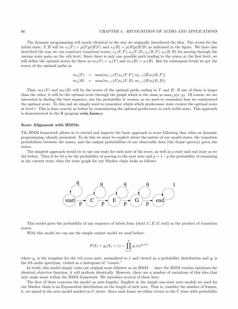
66 CHAPTER 4. RECOGNITION OF AUDIO AND APPLICATIONS
The dynamic programming will nearly identical to the way we originally introduced the idea. The scores for theinitial state, F,B will be s1(F ) = p(F )p(H|F ) and s1(B) = p(B)p(H|B) as indicated in the figure. We have alsodescribed the way we can construct transition scores, sn(F, F ), sn(F,B), sn(B,F ), sn(B,B) for moving through thevarious state pairs on the nth level. Since there is only one possible path leading to the states at the first level, wewill define the optimal scores for these as m1(F ) = s1(F ) and m1(B) = s1(B). But for subsequent levels we got thescores of the optimal paths as
mn(F ) = max(mt−1(F )sn(F, F ),mt−1(B)st(B,F ))mn(B) = max(mt−1(F )sn(F,B),mt−1(B)st(B,B))
Thus, mT (F ) and mT (B) will be the scores of the optimal paths ending in F and B. If one of these is largerthan the other, it will be the optimal score through the graph which is the same as maxx p(x, y). Of course, we areinterested in finding the best sequence, not the probability it creates, so we need to remember how we constructedthe optimal score. To this end we simply need to remember which which predecessor state creates the optimal scoreat level t. This is done exactly as before by remembering the optimal predecessor to each trellis state. This approachis demonstrated in the R program coin hmm.r.
Score Alignment with HMMs
The HMM framework allows us to extend and improve the basic approach to score following that relies on dynamicprogramming, already presented. To do this we must be explicit about the nature of our model states, the transitionprobabilities between the states, and the output probabilities of our observable data (the frame spectra) given thestates.
The simplest approach would be to use one state for each note of the score, as well as a start and end state as wedid before. Then if we let p be the probability of moving to the next note and q = 1− p the probability of remainingin the current state, then the state graph for our Markov chain looks as follows:
start C E G endp p pp
q q q q 1
This model gives the probability of any sequence of labels from start, C,E,G, end as the product of transitionscores.
With this model we can use the simple output model we used before:
P (Yt = yt|Xt = r) =N∏n=1
qr(n)yt(n)
where qr is the template for the rth score note, normalized to 1 and viewed as a probability distribution and yt isthe tth audio spectrum, viewed as a histogram of “counts.”
In truth, this model simply casts our original score follower as an HMM — since the HMM version optimizes theidentical objective function, it will perform identically. However, there are a number of variations of this idea thatonly make sense within the HMM framework. We introduce several of these here.
The first of these concerns the model on note lengths. Implicit in the simple one-state note models we used forour Markov chain is an Exponential distribution on the length of each note. That is, consider the number of frames,L, we spend in the note model marked as C above. Since each frame we either return to the C state with probability

67
q or move on with probability p, we have
P (L = 1) = p
P (L = 2) = qp
P (L = 3) = q2p
......
...P (L = l) = ql−1p
This distribution is often called “Exponential” or “Geometric.” While it may be convenient from a mathematicalperspective, it is certainly not a reasonable model for an actual note length. Imagine a musician who decides at arate of 30 times a second if she will continue to the next note by flipping a biased coin. While this model does capturethe uncertain nature of the situation, the particular kind of uncertainty modeled doesn’t seem musically reasonable.
A more plausible model chains together a collection of m states as in the figure below:
q q
pp p
q
p
q
...
m states
In calculating the distribution on the number of frames spent in this model, let us consider the probabilityP (L = l) — the probability we spend l frames in this model. For L = l to occur, the lth transition must move usout of the model, which happens with probability p. For the remaining l − 1 transitions, m− 1 must move betweenstates (p) while the remaining l−m must state within a state (q). Thus the probability of any particular path that
spends l frames in the model will be p× pm−1 × ql−m = pmql−m. There are (l − 1m− 1 ) such paths since, of the last
l − 1 transitions, we can choose m − 1 of them to be p transitions with the remaining ones q transitions. Thus wehave
p(L = l) =(
l − 1m− 1
)pmql−m
l = m,m + 1, . . . This distribution is known as the “Negative Binomial” distribution. A simple calculation showsthat the mean of this distribution is m/p and the variance is mq/p2. We can choose the number of states in themodel, m, and the parameter p, so that the resulting mean and variance model our belief about this note lengthdistribution. For instance, the mean value could be the length of the note in frames, using the nominal tempo.Better yet, the mean and variance can be estimated from past examples. Estimating the parameters m and p in thisway, by matching the model moments (mean and variance) to the empirical of observed moments, is known as themethod of moments. This is the strategy we employ in practice.
Another improvement is to include features other than our spectrogram. For instance, note attacks are oftensignaled by a sudden burst of energy in the audio data. For repeated pitches, there is virtually no way to identify noteboundaries without identifying some kind of onset event. To do this, we could create a feature that measures this“burstiness” and add on an extra state or two to the beginning of our note model to model this attack. Presumablywhen we visit the attack state, we expect to see more burstiness in the data, while we anticipate less in the remainingstates. This would be captured by using a different output distribution on the burstiness feature for the start of thenote than is used for the other states.

68 CHAPTER 4. RECOGNITION OF AUDIO AND APPLICATIONS
An additional improvement performs the score match not with the optimal path, as we have used until now, butusing the so called forward-backward labeling. While we will omit the details, for a HMM one can compute
p(xt = s|y1, . . . yT )
That is, the distribution on the tth state variable given all of the observable data. This probability distributionrepresents our knowledge about where we are in the Markov model at the tth frame of audio data, having observedall of the audio data. We can then recognize the onset of the kth note as the frame that is most likely to be in thefirst state of the note:
ok = arg maxtp(xt = startk|y1, . . . , yT )
Such a scheme performs better for score following.There are numerous other improvements that can be made to the score alignment HMM, however, in an attempt
to avoid getting bogged down with details, we won’t describe these here. Instead, we will present in class a numberof actual examples of score alignment on highly challenging audio data. This gives a sense of what is possible in thisdomain.
Online Score Following
As we have seen, not all inference with Hidden Markov models is necessarily based on the most likely state sequencex = arg maxx p(x|y). For example, in the filtering problem we compute the distribution on the current state variablegiven the past observations:
p(xt|y1, y2, . . . , yt)
This so-called filtered probability expresses what we know about the current state of the Markov chain given whatwe have seen so far. In some cases we might be reasonably certain about what state we are in — in this case thefiltered distribution will concentrate most of its mass on a single state. In other cases we may be highly uncertain ofthe whereabouts of the chain — in this case the filtered probability may be quite spread out. The ability to makethis distinction is an advantage of probabilistic modeling, since we may be more inclined to take action when we arecertain, yet prefer to wait when we are less certain (remember the boy who cried “wolf”).
If we letαt(i) = p(xt = i|y1, . . . , yt)
we can compute αt through the following recursion:
α1(i) =p(x1 = i)p(y1|x1 = i)∑i′ p(x1 = i′)p(y1|x1 = i′)
(4.2)
αt+1(i) =
∑j αt(j)p(xt+1 = i|xt = j)p(yt+1|xt+1 = i)∑
i′∑j αt(j)p(xt+1 = i′|xt = j)p(yt+1|xt+1 = i′)
(4.3)
In this expression for αt+1(i) the denominator is just the normalizing constant needed to make the expression aprobability distribution — though both i′ and j appear in this expression, these variables are just summation indicesand not actual variables like i in the numerator.
To see the correctness of the formula, note that by simple rules of probability
αt+1(i) = p(xt+1 = i|y1, . . . , yt, yt+1)
= p(xt+1 = i, yt+1|y1 . . . , yt)p(y1, . . . , yt)p(y1, . . . , yt+1)
∝ p(xt+1 = i, yt+1|y1, . . . , yt) (viewed as a function of i)
=∑j
p(xt+1 = i, xt = j, yt+1|y1, . . . , yt)
=∑j
p(xt = j|y1, . . . , yt)p(xt+1 = i|xt = j, y1, . . . , yt)p(yt+1|xt = j, xt+1 = i, y1, . . . , yt)
=∑j
αt(j)p(xt+1 = i|xt = j)p(yt+1|xt+1 = i)

69
Since αt+1(i) is a probability distribution it must sum to 1. Thus if we divide the right-hand-side by theappropriate constant to make it sum to 1 we have equality rather than just proportionality. Eqn. 4.3 simply addsappropriate denominator to make this happen.
To imagine this formula in action in the score following context, consider an HMM with Markov chain as in thefollowing figure:
Rest
Note1
Note 2
Note 3
Each iteration of the forward algorithm (the calculation of the αt probabilities) advances one step by computing
αt+1(i) =
∑j αt(j)QjiRiyt+1
normalizing constant
where, in our simplified notation, Qji is the transition probability of going from state j to state i and Riyt+1 is theprobability of observing the t+ 1th frame of data, yt+1 given we are in state i.
We will initialize our model with p(x1 = init rest) = 1 so that for the first frame of audio α1(i) concentrates allof its probability mass on the initial rest state. Imagine now that we start by receiving a sequence of frames that areconsistent with the rest state. This means that Riyt is high when i is the rest state but lower otherwise. In this case,even though the αt probabilities generate hypotheses that move forward through the state graph, after multiplyingby the data probability, only the hypothesis of the rest state will have any significant amount of probability mass.Thus αn(i) will continue concentrating its probability mass on the rest state as long as our audio data are consistentwith the rest assumption.
Eventually we will see audio data that is consistent with the first note of the piece. When this first happens thestate at the start of the 1st note will have significant probability after the forward iteration is computed. As wecontinue to get audio data consistent with the first note, probability mass begins to propagate through the first note.Since the first two transitions of the note are deterministic (have probability 1) we know that two frames later all ofthe probability mass will have moved forward to the first state with the self-loop of note 1. As we continue to getaudio data consistent with the 1st note, this mass propagates forward through the chain of self-loops. Since all ofthese state have the same observation probability, this propagation only depends on the transition probabilities. If pis the probability of moving forward, p percent of the probability mass of each state moves to the next state in eachiteration. One can think of this as a “bulge” that moves through the sequence of states until, after the appropriatenumber of frames, it begins “knocking on the door” of the next note. Thus the model is poised to recognize the

70 CHAPTER 4. RECOGNITION OF AUDIO AND APPLICATIONS
next note after the first note has sounded for the appropriate amount of time. During this period if we get modestevidence of the 2nd note, probability mass will easily slide into the 2nd note model. However, if the audio dataconfirms that we are still in the first note, the probability mass that sneaks into the 2nd note will be decreased tonothing by the output probabilities.
Thus probability mass continues to move through our network of state, most easily transitioning from one noteto the next after an appropriate amount of time spent in the current note, but always bound to be consistent withthe audio data.
Our score follower provides a running commentary on the audio data, pinpointing the onsets of notes and commu-nicating these estimates during the performance. This works as follows. Suppose we have observed notes 1, 2, . . . , k−1and are currently waiting to see the kth note. We continue computing the forward probabilities until
p(xt ≥ startk|y1, . . . , yt)
is sufficiently large where startk is the first state of the kth note. That is, we wait until we are reasonably certainthat we have passed the onset of the kth note. Note that this computation is easily done using the α probabilities —we simply add up all α probabilities for states that are beyond the start of the kth note. Eventually this probabilitywill be large enough for us to be confident that the kth note has sounded — say that t∗ is the time (frame) at whichthis level of certainty occurs.
At this point we look backwards in time (look at t ≤ t∗) and for each such frame compute
p(Xt = startk|y1, . . . , yt∗)
Note that we are using all of the data up to t∗ to do this. While we haven’t discussed the mechanics of thiscomputation, it is easy to do with HMMs. Intuitively, this is exactly what we want to do. Having determined thatthe onset of the kth note is in the past, let’s look backward to see where we think it began. While many estimationtechniques are possible, we choose the frame t where the note is most likely to begin. That is we estimate the onsetof the kth note by
ok = arg maxt≤t∗
P (Xt = startk|y1, . . . , yt∗)
In class we will show a real-time demonstration of the way in which this calculation works. It is important to notethat there will always be latency built into this estimation problem, since we can’t detect a note until we alreadyhave some evidence for its existence.
Musical Accompaniment Systems
A musical accompaniment system is a program that provides an accompaniment to a live player in a piece of musicfor soloist and accompanying ensemble. Our particular flavor of the problem deals with non-improvisatory “classical”music such as a concerto for violin and orchestra.
The problem can be motivated by the familiar “Music Minus One” play-along records that provide (mostly)orchestral accompaniments to familiar solo repertoire. While these records are a nice introduction to the experienceof the orchestral soloist, they do not capture the experience very faithfully. Common musical thinking dictates thatthe orchestra should follow the soloist, which, of course, cannot happen with a recorded accompaniment. One canthink of the musical accompaniment system as trying to turn this around so the orchestra follows the soloist.
There are three principal ingredients to such as system:
1. Real time score following
2. Phase vocoded audio output (or midi output)
3. Accompaniment control (the brain of the system).
We have already talked about real time or online score following. We have also talked about phase vocoding,which can be used to generate an audio accompaniment by warping the playback rate to match the soloist. Of course,there are other ways that the accompanying sound can be generated. The final component is a musical brain thatuses the note onset times provided by the score follower to drive the performance of the accompaniment. While thissubject doesn’t obviously fit into a class on audio, it doesn’t seem to belong in any other class I can think of either.So I will discuss it here.
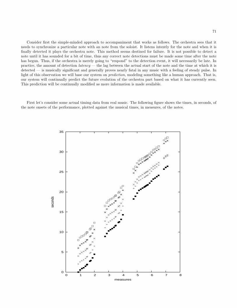
71
Consider first the simple-minded approach to accompaniment that works as follows. The orchestra sees that itneeds to synchronize a particular note with an note from the soloist. It listens intently for the note and when it isfinally detected it plays the orchestra note. This method seems destined for failure. It is not possible to detect anote until it has sounded for a bit of time, thus any correct note detections must be made some time after the notehas begun. Thus, if the orchestra is merely going to “respond” to the detection event, it will necessarily be late. Inpractice, the amount of detection latency — the lag between the actual start of the note and the time at which it isdetected — is musically significant and generally proves nearly fatal in any music with a feeling of steady pulse. Inlight of this observation we will base our system on prediction, modeling something like a human approach. That is,our system will continually predict the future evolution of the orchestra part based on what it has currently seen.This prediction will be continually modified as more information is made available.
First let’s consider some actual timing data from real music. The following figure shows the times, in seconds, ofthe note onsets of the performance, plotted against the musical times, in measures, of the notes.
0
5
10
15
20
25
30
35
0 1 2 3 4 5 6 7 8
seco
nds
measures

72 CHAPTER 4. RECOGNITION OF AUDIO AND APPLICATIONS
In the figure each of the performances are “stacked” vertically for easy comparison. If such a performance wereplayed completely in time, with each actual note length proportional to the note value given in the score, then thepoints would lie on a line. Clearly this is not the case. This particular example shows a common syndrome inmusical performance: the tempo is gradually increased over the first several notes to “ease into” the basic tempo,while the tempo slows down at the end of the phrase. This non-metronomic aspect makes it particularly difficult tofollow such a musical interpretation. However, one can also see that there is a good deal of commonality between theperformance, so that we may hope to learn from past performances in predicting the timing evolution of the currentperformance.
Here is a possible model for the musical timing in a piece of music. We let tk denote the time, in seconds, thatthe kth note begins and sk be the tempo, in seconds per beat, for the kth note.
sk+1 = sk + σk
tk+1 = tk + lksk + τk
In the model above, lk is the length of the kth note in beats, thus the product lksk is the time, in seconds, allotedto the kth note according to the local tempo, sk. The variables σk and τk allow the model to be more flexible andto capture human aspects of interpretation. For instance, if σk > 0 this means that the tempo (in secs/beat) isincreasing at the kth note, thus we are slowing down. Similarly, a negative value of σk denotes a local speeding upof tempo. The τk variables capture variations in note length that cannot be explained by tempo, such as in the caseof a single note that is elongated without any decrease in tempo, as in an agogic accent.
More formally the pair σk, τk are modeled as Gaussian variables:
τk ∼ N(µτk, ρ2τk
)
σk ∼ N(µσk, ρ2σk
)
where τk, σk are a collection of independent random variables. In this notation N(µ, ρ2) denotes a normal distri-bution with mean µ and variance ρ2. With this modeling, µτk
gives the average tempo change at a particular notewhile ρ2
τkexpressed the repeatability of this tempo change — is it nearly the same way every time (small ρ2
τk) or is
it more variable from time to time (large ρ2τk
). Similar interpretations can be made of the mean and variance of theσk distribution.
The above model describe the time evolution of a single musical voice with a time varying tempo, “driven” bya collection of random variables. We now wish to treat the solo and accompaniment parts together. To this end,we will employ the model just discussed on the composite rhythm — the rhythm achieved by overlaying the musicalparts. For instance, consider the two rhythms for solo and accompaniment described below:
Solo
Accomp
3 3
This musical notation means that there are three evenly spaced notes in the solo part for every two evenly spacednotes in the accompaniment. In such a situation the two parts play some of the notes together (every 3rd note forthe solo and every 2nd note for the accompaniment), while the others are not synchronous. This rhythm is expressedin our model by the following graph structure.

73
Listen
Composite
Updates
Accomp
The expression of a probability distribution as a directed (with arrows) acyclic (no circuits) graph is a commonway of expressing a probability distribution. The meaning of such a graph is essentially a factorization of the jointprobability distribution on all variables. That is, the joint distribution is expressed as a product of conditionaldistributions, one for each graph node, in which the variables associated with the graph node depend only on their“parents” in the graph.
In interpreting this graph, the middle layer is the collection of time and tempo (tk, sk) variables for the compositerhythm describes by the model. The layer labeled as “update” are the random variables σk, τk that “drive” themodel. The top layer of variables are the observed onset times estimated by the score following module while thelowest layer in the graph are the onset times of the accompaniment notes.
Our model facilitates a number of calculations that will be of interest to us, which we describe here. Each ofthese requires we compute the distribution on some of the unobserved variables of the model, given that we haveobserved other variables in the model. The mechanics of these computations will remain outside the scope of thiscourse, though they are standard calculations for probabilistic graphical models and Bayesian belief networks.
The first problem is one problem we have already seen: given the complete solo performance, performed inisolation, how do we construct an orchestral accompaniment that fits to this. When discussed before we showedhow phase vocoding could be used to warp and existing orchestral performance to fit the solo performance. Here wediscuss the computation of the times at which the orchestra should play its notes. When we are given the soloist’stimes in our model we depict this by darkening in the circles corresponding to the observations, as below.
Listen
Composite
Updates
Accomp
Given this information we can compute the conditional distribution on each of the variable corresponding toorchestra times. These times depend on the observed solo times, the raw score information, which is embedded inthe model, and the nature of the “update” variables that capture the expression exhibited in past performances. Wehave already seen an application of this idea in our section of phase vocoding.
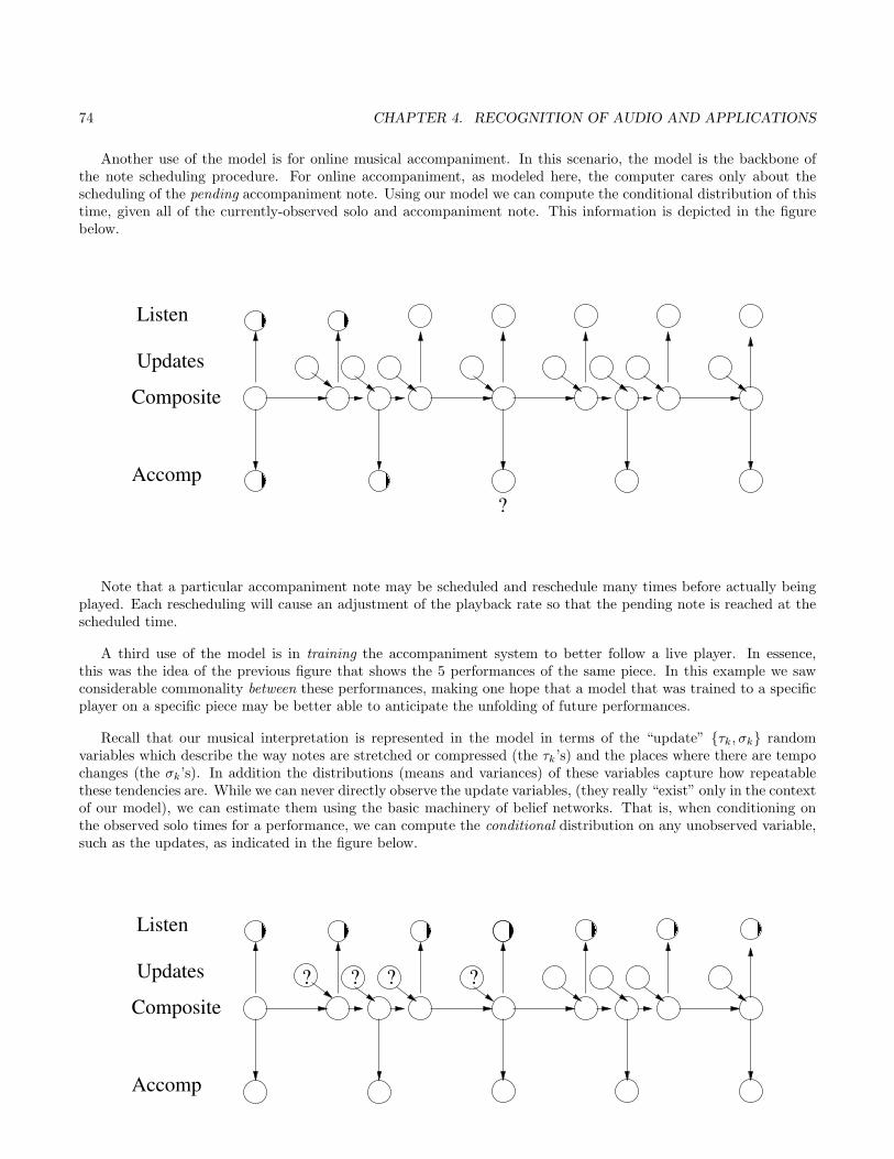
74 CHAPTER 4. RECOGNITION OF AUDIO AND APPLICATIONS
Another use of the model is for online musical accompaniment. In this scenario, the model is the backbone ofthe note scheduling procedure. For online accompaniment, as modeled here, the computer cares only about thescheduling of the pending accompaniment note. Using our model we can compute the conditional distribution of thistime, given all of the currently-observed solo and accompaniment note. This information is depicted in the figurebelow.
Listen
Composite
Updates
Accomp?
Note that a particular accompaniment note may be scheduled and reschedule many times before actually beingplayed. Each rescheduling will cause an adjustment of the playback rate so that the pending note is reached at thescheduled time.
A third use of the model is in training the accompaniment system to better follow a live player. In essence,this was the idea of the previous figure that shows the 5 performances of the same piece. In this example we sawconsiderable commonality between these performances, making one hope that a model that was trained to a specificplayer on a specific piece may be better able to anticipate the unfolding of future performances.
Recall that our musical interpretation is represented in the model in terms of the “update” τk, σk randomvariables which describe the way notes are stretched or compressed (the τk’s) and the places where there are tempochanges (the σk’s). In addition the distributions (means and variances) of these variables capture how repeatablethese tendencies are. While we can never directly observe the update variables, (they really “exist” only in the contextof our model), we can estimate them using the basic machinery of belief networks. That is, when conditioning onthe observed solo times for a performance, we can compute the conditional distribution on any unobserved variable,such as the updates, as indicated in the figure below.
Listen
Composite
Updates
Accomp
?? ? ?

75
While we cannot observe the updates directly, we can compute their conditional mean times and use this asa substitute for direct knowledge. For instance, a natural estimate of the mean and variance of for one of thesevariables, say τk, would be to take the empirical mean and variance of the collection τk estimates (the conditionalmeans) taken over a collection of performances. The estimation technique we will employ is a variation on this ideaknown as the EM algorithm, though we will not present the details here.
We will demonstrate in class the results of this kind of training technique in an actual performance situation.
New Music for Acoustic Instrument and Electronica
Music Transcription (Signal to Score)
The goal of music transcription is to transform an audio signal into a score-like symbolic representation as below:
In the most ambitions version of this problem we would like to recover the pitches, rhythms, instruments, voices,etc. for a piece of polyphonic music such as an orchestra, rock band, percussion ensemble, etc.
Possible applications of transcription include:
1. Create searchable, analyzable, printable symbolic database of any music genre. Searchability here may appealto a music listener or librarian who wants to find a particular fragment of music — in essence, this seeks to be“Google for music.” The analyzable aspect may appeal to a musicologist who wants to be more quantitativein the study of music than previous eras have allowed. The printable aspect will likely appeal to performs whowould like to play the music. It is worth mentioning an argument against this approach, however. Opticalcharacter recognition for music is likely a much easier problem (though still quite challenging) This may be afaster way to assemble the desired symbolic databases for music that exists in printed form.
2. Capturing unnotated and improvisatory music, such as jazz or musics that are transmitted through an auraltraditions.
3. This problem is a terrific intellectual challenge related to deep cognitive questions, (like how to model music).
4. Your answer here.
It is possible that the short term successes of transcription will be less important that those of score following, thoughthere is much to offer here too.
Simply trying to pose the problem of transcription is a challenging task. The main difficulty here is in finding asimplification that allows practical solution, but not so simplified that the solutions are useless. In general this is animportant aspect of much applied work. Here are some possible candidates:
1. Monophonic audio to score (as in “query by humming”).
2. Audio to piano roll representation (discrete pitch and continuous start and stop times for notes).
3. Single instrument to score (piano, guitar, mbira, etc.)
4. Audio to chord sequence
5. rhythm transcription given onset times.

76 CHAPTER 4. RECOGNITION OF AUDIO AND APPLICATIONS
Of these the easiest is monophonic piano roll transcription in which we seek to partition an audio stream into segmentslabeled with a pitch or a rest. We will discuss this problem in a little more detail here.
To begin, recall the methods we discussed for the pitch recognition of a single frame. These were templatematching, in which we seek the pitch or rest label tk giving the best match to an audio frame s:
k = arg maxk
s · tk
or our maximum likelihood technique in which we sought the model tk giving the highest probability to that data.This turned out to be the same as solving
k = arg maxk
s · log tk
We saw that this technique performed okay for single frames but still made plenty of mistakes. The idea here is thatnow we seek a sequence of frame labels. How can we restrict our attention to sequences that make musical sense, or,at least, how can we bias our approach to favor musically plausible sequences.
For instance, suppose we run a frame recognizer and find it produces the sequence:
CC]CCBCCCCCC]DE[DDDC]DDDD . . .
It is, of course, impossible to have notes composed of single frames. A more likely interpretation would be
CCCCCCCCCCC|DDDDDDDDDD . . .
HMM Approach (hmm mono recog.r)
Suppose we begin with a known note length probability distribution, in frames. Possible examples are given belowwhere we assume a uniform distribution on note length, a more realistic distribution when both tempo and notevalue are known, and a third example that uses a multi-modal (several modes = peaks) trying to model the situationwhen we don’t know the note value.
len
p(len)
all lengths in range =’ly likely
assuming constant note valueand known tempo
a multi−model model for knowntempo but unknown note value
1/16 1/8 3/16

77
In all of these cases it is easy to build a model that captures the note length. If the note length distribution, inunits of frames, is given by q(l), with q(l) possibly equal to 0 for some values and with maximal value lmax, then wecan construct the distribution through a collection of states s1, s2, . . . , slmax where state sl represents the situationin which the note is greater than l frames long. Thus we will only allow transitions from state sl and states sl+1 andslmax with the transition probabilities
p(sl+1|sl) = p(len ≥ l + 1|len ≥ l)
=∑k>l+1 q(k)∑k>l q(k)
and
p(slmax |sl) = 1− p(sl+1|sl)
The topology of this model is depicted below.
1 2 3 4 5 lmax
Once we have constructed such a note length model, we build a different instance of it for every possible pitch.Denoting these first and last states of these models in the diagrams below, we can form a “completely connected”graph that allows every possible pitch to follow every possible pitch as depicted below.
60
...
61
62
63 ...
...
...
...
78 CHAPTER 4. RECOGNITION OF AUDIO AND APPLICATIONS
With the model in place, dynamic programming can be used to find the most likely path, given the data, usinga data model such as the one already presented. A demonstration of this approach can be found in the programhmm mono recog.r.
Polyphonic Transcription
Polyphonic transcription tries to automatically represent music consisting of several independent parts. This problemseems to be more difficult than monophonic transcription by orders of magnitude.
For one, in monophonic transcription there are only a small number of possible note hypotheses, since a mono-phonic instrument only produces a small number of notes, say around 50. Furthermore, the audio signatures ofmany of these notes are quite dissimilar from one another, making certain distinctions easy to make. In polyphonictranscription, on the other hand, several notes may sound at once, leading to a large number of possible “chords” or“simultaneities.” For example, if four instruments each play one of 50 notes, we have 50× 50× 50× 50 = 6, 250, 000possible configurations. To make matters worse, many of these are virtually indistinguishable using the kinds oftechniques we have discussed. For instance, if both the notes C4 (middle C) and C5 sound at the same time, we onlyobserve energy lying in the harmonic series of C4 — the C5 contribution is a subset of C4. There are many differentcombinations of pitches that lead to identical frequency signatures, sometimes known as “homonyms.” This termsusually refers to two words that sound alike but are spelled differently, such as aisle, I’ll and isle, but is also aptwith pitch recognition. Perhaps, more to the point, many of these pitch configurations may not be identical, but arequite close to on another, making subtle distinctions quite challenging.
Due to the difficulty with polyphonic recognition, it is not surprising that a good deal of effort has focused onsimpler problems that may be someday be pieces of a larger solution. Chord Identification is one example of thisthat has received a fair amount of attention in recent years. The idea here is simply to take a single audio spectrum,presumed to come from a single pitch configuration, and to identify the constituent pitches. A typical approach herewould iteratively assemble a chord hypothesis in a “greedy” manner. That is, given an audio magnitude spectrum,s, we search for the single note spectrum tk maximizing some measure of closeness s · log tk. We can let
k1 = arg maxk
s · log tk
Then we proceed to try all other notes that can be added to k1. We can approximate the effect of two simultaneousnotes simply by averaging their magnitude spectra: (tk + tk′)/2. While the effect of two simultaneous notes is notreally additive, it is difficult to come up with a more reasonable assumption due to the unknown nature of theinterference between harmonics. Thus we could seek a 2nd pitch k2 by
k2 = arg maxk
s · log(tk1 + tk)/2
The general idea is to continue adding in more pitches until we can no longer improve the data score.In practice, approaches like this may perform acceptably in some cases, but generally fall far short of “solving”
the problem. In fact, there are no present approaches to polyphonic music recognition that seem all that promisingif human abilities are the measure of success. There are several reasons why this may be the case.
One possibility is that we simply have not found the right way to represent the data. The spectrogram is anintuitively appealing representation, since, at first, it seems to capture so much of what we hear. Certainly oneaspect of human hearing follows frequency content over time. However, the spectrogram fails to represent the phaseinformation between frames that may be crucial to how we actually hear: musical sounds are so often objects thatevolve continuously in amplitude, frequency, and phase. Perhaps a representation that decomposes the originalsound into such continuously-varying building blocks may prove more useful for recognizing music. At any rate, thequestion of the basic data representation remains open.
Another school of thought looks at the great amount of human knowledge we bring to music recognition. Muchof this knowledge understands musical behaviors that “make sense” and are thus likely explanations. Repetition is aprime example of this kind of knowledge. A voice or musical part that moves back and forth between two pitches islikely to continue doing so. There are many generalizations of the notion of repetition, and all of these are integralto the kinds of expectations people have about how music will evolve. Other examples of human understanding andexpectation happen on bigger time scales. For instance, much music is tonal, meaning that there is a certain mostimportant note, and usually a corresponding “scale” of pitches. This creates strong beliefs in the listener about whatnotes makes sense in a tonal context. Perhaps music recognition that simultaneously recognizes such a tonal context

79
— say the key — may give better results. The same can be said about rhythmic considerations which also produceexpectations on the listener’s part. The simplest such example would be meter. Metered music decomposes musicinto units called measures where every measure contain the same amount musical time (beats). Typically thereare patterns that appear at the same position in the measure as well. Simultaneously recognizing such high-levelrhythmic notions may also improve our ability to transcribe music.
While simultaneously recognizing such musical structure may lead to better results, it also carries an addedcomputation burden with it. While I personally believe this may well be the key to producing better recognitionresults, it would be fair to say there is not much evidence to back up this belief. Clearly, the polyphonic recognitionproblem remains open, and may continue so for a long time.
Precise Estimation of Pitch
As we have discussed, a Fourier transform of a pitched sound produces peaks around the harmonics. Both the lowestpeak and the spacing between the peaks give the “fundamental” frequency, which we hear as the pitch of the sound.For instance, the figure below shows a typical magnitude spectrum for a pitched sound, with a “blowup” of the regionaround the fundamental peak.
f 2f 3f etc
kblowup around fundamental peak
complete spectrum
From this picture we would be inclined to estimate the pitch of the sound by taking the “bin,” k, giving themaximum amplitude,
k = arg maxk|X(k)|
where X(k) is the Fourier transform, and estimating the frequency, in Hz, by
kcycles
FFT length= k
cyclesN/SR secs
=k · SRN
cyclessec
Since k is an integer, our estimate is only accurate to SR/N Hz. For example, if we choose a sampling rate of 8kHz with 1024 points per FFT, our estimate would be accurate to 8000
1024 ≈ 8 Hz. What if we need a more accurateestimate?
Autocorrelation (autocor.r)
The autocorrelation looks at the “dot product” of the signal with shifted copies of itself. More precisely, theautocorrelation at “lag” r, for r = 0, 1, . . . , computes the dot product of the signal and the signal shifted by rsamples. That is, if the signal is x0, x1, . . . , xN−1 the autocorrelation is given by
a(r) =1N
∑n
xnxn+r

80 CHAPTER 4. RECOGNITION OF AUDIO AND APPLICATIONS
for r = 0, . . . , N − 1. As with the discrete convolution discussed before, we take n+ r to mean the sum modulo N .The autocorrelation is useful for detecting periodicities in the signal. To see this note that when a signal has
period r samples, then a(r) will be a dot product of the signal with itself. By the same reasoning employed fortemplate matching, a(r) will be the maximal value of the autocorrelation (along with a(0), a(2r) etc.). Thus we findperiodicities by looking for peaks of the autocorrelation.
To find the frequency in Hz suggested by the autocorrelation, a, suppose
r = arg maxr>0
a(r)
Then the frequency of the signal will be
rsamplescycle
=r
SR
secscycle
=SR
r
cyclessec
Thus the possible frequency estimates are SR/r for r = 1, 2, 3, . . . , N . Notice that the autocorrelation does notproduce uniform frequency resolution, with better resolution for low frequencies with longer period (large r). However,both the autocorrelation and the Fourier method described above suffer from the discrete nature of the estimate,either in terms of frequency bins, or lag.
While we will not give an explanation, there is an interesting connection between the autocorrelation, a(r) andthe FFT X. That is, if we let
aFFT←→ A
xFFT←→ X
then we have A(k) = X(k)X(k) = |X(k)|2, where X denotes complex conjugate. The FFT of the autocorrelation isthe squared modulus of the signal FFT.
Estimating Frequency using the Definition
Suppose we have a sampled sinusoid that oscillates at 1 cycle per FFT length. Imagine that we compute the STFTusing a hop size of N/H where N is the FFT length. For each computed FFT, we will see a strong peak at bin 1;but what will happen with the phase at this peak? Since the signal oscillates at 1 cycle per N points, we will see thephase advancing by increments of 2π
H each FFT. From this one can see that the phase advance per hop is directlyproportional to the frequency of the signal. Thus we could compute the frequency by computing the phase advanceper hop, divided by the time associated with the hop. In other words, frequency is the rate of change or derivativeof phase divided by 2π:
2πf(t) =d
dtφ(t)
We can use this idea to estimate frequency directly from this definition. Suppose we observe a peak in our signalat bin k. We have already seen that a crude estimate of the frequency is k SRN Hz. To get a more precise estimatesuppose that the next FFT is computed after “hopping” N samples. If the frequency were exactly k cycles perFFT length, we would see the same phase at the adjacent FFT for bin k. However, a more accurate estimate of thenumber of cycles traversed would be k + (φ2(k)− φ1(k))/2π where φ1(k) and φ2(k) are the phases for bin k on thetwo transforms. This leads to the frequency estimate
f =k + (φ2(k)− φ1(k))/2π
N/SR
In interpreting this formula, the difference φ2(1)−φ1(1) is always taken to be a number in (−π, π] — In other words,we assume that k is the best integer approximation to the number of cycles traversed between frames.
This same idea can be extended to the case with hop size N/H, and, in fact the estimation is usually more accurateas H increases. Suppose k is the bin containing a peak for two adjacent overlapping FFTs with hop N/H. If k werethe exact frequency (in cycles per FFT length) we would expect the phase to advance by 2πk/H between the twoframes. Thus, a more precise estimate of the phase traversed in this time window is 2πk+ (φ2(k)−φ1(k))− 2πk/H.This leads to the frequency estimate
f =2πk/H + ((φ2(k)− φ1(k))− 2πk/H)π−π
2π(N/H)/SR

81
Here we denote the “principal argument” (∆)π−π as the angle ∆ viewed as lying in the range (−π, π]. That is
(∆)π−π = ((∆ + π) mod 2π)− π