Chronicle of a Decline Foretold: Has China Reached the Lewis Turning Point?

Mitali Das and Papa N’Diaye

WP/13/26

© 2013 International Monetary Fund WP/13/26

IMF Working Paper

Research Department and Asia and Pacific Department

Chronicle of a Decline Foretold: Has China Reached the Lewis Turning Point?

Prepared by Mitali Das and Papa N’Diaye

Authorized for distribution by Steven Phillips and Steven Barnett

January 2013

Abstract

China is on the eve of a demographic shift that will have profound consequences on its economic and social landscape. Within a few years the working age population will reach a historical peak, and then begin a precipitous decline. This fact, along with anecdotes of rapidly rising migrant wages and episodic labor shortages, has raised questions about whether China is poised to cross the Lewis Turning Point, a point at which it would move from a vast supply of low-cost workers to a labor shortage economy. Crossing this threshold will have far-reaching implications for both China and the rest of the world. This paper empirically assesses when the transition to a labor shortage economy is likely to occur. Our central result is that on current trends, the Lewis Turning Point will emerge between 2020 and 2025. Alternative scenarios—with higher fertility, greater labor participation rates, financial reform or higher productivity—may peripherally delay or accelerate the onset of the turning point, but demographics will be the dominant force driving the depletion of surplus labor.

JEL Classification Numbers: C3, C18, J11, J2, J61, O17

Keywords: Excess labor supply, Lewis Turning Point, Population aging, Demographics

Author’s E-Mail Address: mdas@imf.org; pndiaye@imf.org

This Working Paper should not be reported as representing the views of the IMF. The views expressed in this Working Paper are those of the author(s) and do not necessarily represent those of the IMF or IMF policy. Working Papers describe research in progress by the author(s) and are published to elicit comments and to further debate.

2

Contents Page

I. Introduction ............................................................................................................................3 

II. Recent Developments ............................................................................................................5 

III. Empirical Framework ..........................................................................................................7 

IV. Results................................................................................................................................10 

V. Scenario Analysis ................................................................................................................12 A. Baseline Scenario ....................................................................................................12 B. Increase in the Fertility Rate ...................................................................................15 C. Higher Labor Force Participation Rates ..................................................................16 D. Financial Sector Reform .........................................................................................16 E. Product Market Reform ...........................................................................................16 

VI. Conclusion .........................................................................................................................17 

References ................................................................................................................................19  Appendix: Derivation of Empirical Framework ......................................................................18 

3

I. INTRODUCTION

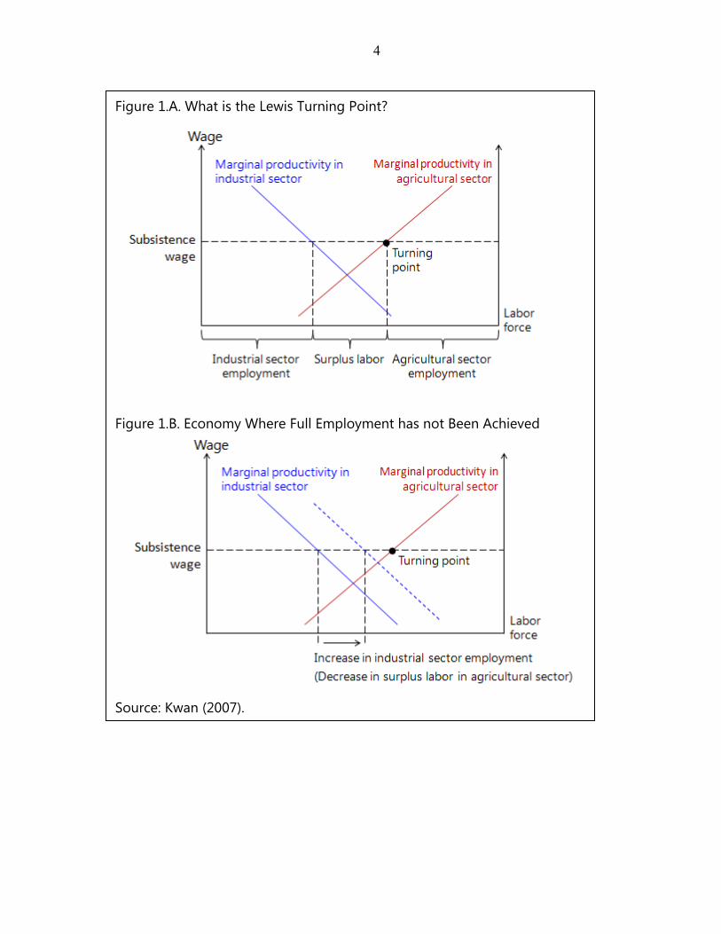
China’s large pool of surplus rural labor has played a key role in maintaining low inflation and supporting China’s extensive growth model. In many ways, China’s economic development echoes Sir Arthur Lewis’ model, which argues that in an economy with excess labor in a low productivity sector (agriculture in China’s case), wage increases in the industrial sector are limited by wages in agriculture, as labor moves from the farms to industry (Lewis, 1954). Productivity gains in the industrial sector, achieved through more investment, raise employment in the industrial sector and the overall economy. Productivity running ahead of wages in the industrial sector makes the industrial sector more profitable than if the economy was at full employment and promotes higher investment. As agriculture surplus labor is exhausted, industrial wages rise faster, industrial profits are squeezed, and investment falls. At that point, the economy is said to have crossed the Lewis Turning Point (LTP) (Figure 1). Anecdotal evidence of rapid nominal wage increases and episodic labor shortages have raised questions about whether the era of cheap Chinese labor is coming to an end and whether China has reached the LTP. China’s crossing the LTP would have consequences for both China and the rest of the world. For China, this would mean that the current extensive growth model that relies so heavily on factor input accumulation could not be sustained and that China would need to invest less, but in better, capital. This would imply switching to a more ‘intensive” growth model with a greater reliance on improving total factor productivity (TFP), which in essence means accelerating the implementation of the government’s agenda to rebalance growth away from investment toward private consumption. Successfully rebalancing China’s growth pattern would yield significant positive external spillovers to the rest of the world, potentially raising output particularly in those countries within the supply chain (mainly emerging Asia) and commodity exporters, and somewhat more limited spillovers to advanced economies (IMF, 2011). Moreover, rising labor costs—whose impact will be felt on prices and corporate profit margins in China—will have implications for trade, employment and price developments in key trading partners. Against this backdrop, this paper presents estimates of China’s excess labor supply using a general procedure developed in Rosen and Quandt (1978, 1986) and Rudebusch (1986). The empirical model attributes an explicit role to population composition, labor force participation and the productivity—characteristics of the Chinese labor market most likely to be relevant in an analysis of excess supply. The remainder of the paper is organized as follows: Section II provides a brief overview of recent trends in China’s labor market; Section III presents the empirical framework; baseline results are given in Section IV; Section V presents scenario analysis around a central baseline forecast of future trend in the labor market; and Section VI concludes.

4

Figure 1.A. What is the Lewis Turning Point?

Figure 1.B. Economy Where Full Employment has not Been Achieved

Source: Kwan (2007).

5

II. RECENT DEVELOPMENTS

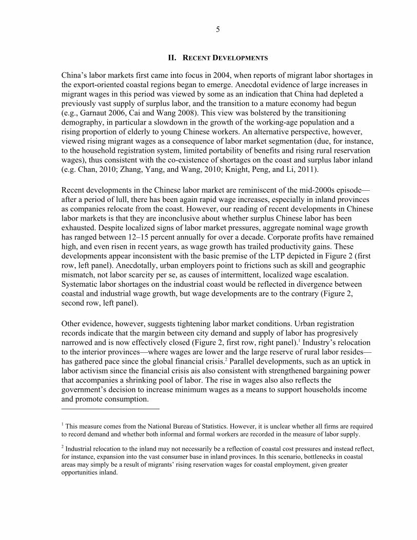
China’s labor markets first came into focus in 2004, when reports of migrant labor shortages in the export-oriented coastal regions began to emerge. Anecdotal evidence of large increases in migrant wages in this period was viewed by some as an indication that China had depleted a previously vast supply of surplus labor, and the transition to a mature economy had begun (e.g., Garnaut 2006, Cai and Wang 2008). This view was bolstered by the transitioning demography, in particular a slowdown in the growth of the working-age population and a rising proportion of elderly to young Chinese workers. An alternative perspective, however, viewed rising migrant wages as a consequence of labor market segmentation (due, for instance, to the household registration system, limited portability of benefits and rising rural reservation wages), thus consistent with the co-existence of shortages on the coast and surplus labor inland (e.g. Chan, 2010; Zhang, Yang, and Wang, 2010; Knight, Peng, and Li, 2011). Recent developments in the Chinese labor market are reminiscent of the mid-2000s episode—after a period of lull, there has been again rapid wage increases, especially in inland provinces as companies relocate from the coast. However, our reading of recent developments in Chinese labor markets is that they are inconclusive about whether surplus Chinese labor has been exhausted. Despite localized signs of labor market pressures, aggregate nominal wage growth has ranged between 12–15 percent annually for over a decade. Corporate profits have remained high, and even risen in recent years, as wage growth has trailed productivity gains. These developments appear inconsistent with the basic premise of the LTP depicted in Figure 2 (first row, left panel). Anecdotally, urban employers point to frictions such as skill and geographic mismatch, not labor scarcity per se, as causes of intermittent, localized wage escalation. Systematic labor shortages on the industrial coast would be reflected in divergence between coastal and industrial wage growth, but wage developments are to the contrary (Figure 2, second row, left panel). Other evidence, however, suggests tightening labor market conditions. Urban registration records indicate that the margin between city demand and supply of labor has progresively narrowed and is now effectively closed (Figure 2, first row, right panel).1 Industry’s relocation to the interior provinces—where wages are lower and the large reserve of rural labor resides—has gathered pace since the global financial crisis.2 Parallel developments, such as an uptick in labor activism since the financial crisis ais also consistent with strengthened bargaining power that accompanies a shrinking pool of labor. The rise in wages also also reflects the government’s decision to increase minimum wages as a means to support households income and promote consumption. 1 This measure comes from the National Bureau of Statistics. However, it is unclear whether all firms are required to record demand and whether both informal and formal workers are recorded in the measure of labor supply.

2 Industrial relocation to the inland may not necessarily be a reflection of coastal cost pressures and instead reflect, for instance, expansion into the vast consumer base in inland provinces. In this scenario, bottlenecks in coastal areas may simply be a result of migrants’ rising reservation wages for coastal employment, given greater opportunities inland.

6

Figure 2. Labor Market Developments

-10

0

10

20

-10

0

10

20

2000Q1 2002Q1 2004Q1 2006Q1 2008Q1 2010Q1 2012Q1

Unit labor cost* (4Qma, yoy growth)Nominal average wages (4Qma, yoy growth)

Unit Labor Cost and Nominal Wages

* Imputed total wages for 2011Q4.

0.6

0.7

0.8

0.9

1

1.1

2001 2002 2003 2004 2005 2006 2007 2008 2009 2010 2011

City Labor: Demand/Supply

5

10

15

20

25

5

10

15

20

25

2008Q1 2008Q3 2009Q1 2009Q3 2010Q1 2010Q3 2011Q1 2011Q3

Coastal

Interior

Wage Growth: Coastal vs. Interior(In percent)

-10

-5

0

5

10

15

20

1950 1960 1970 1980 1990 2000 2010 2020 2030 2040 2050

Growth of Working Age Population(In percent)

0

0.2

0.4

0.6

0.8

1955 1965 1975 1985 1995 2005 2015 2025 2035 2045

Dependency Ratio

-80000 -60000 -40000 -20000 0 20000 40000 60000 80000

0-4

10-14

20-24

30-34

40-44

50-54

60-64

70-74

80+

85-89

95-99 Female

Male

Population Pyramid, 2030

7

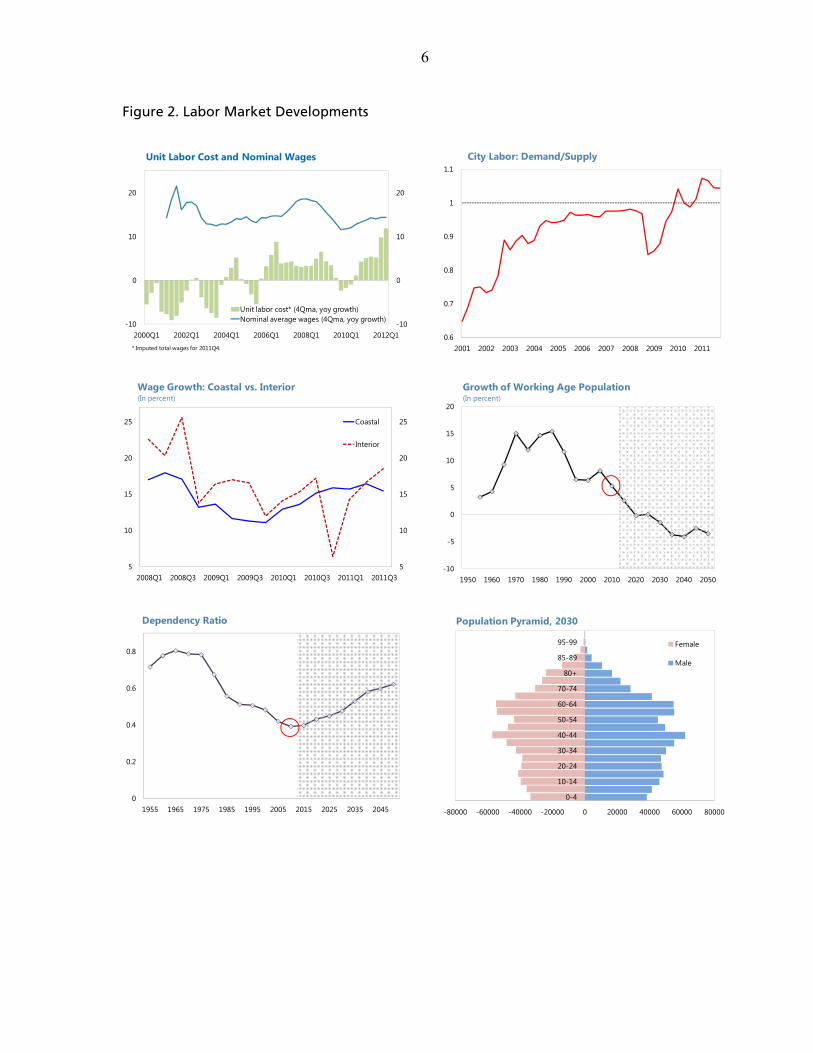
Thus overall, labor market developments paint a mixed picture about excess labor: wage developments do not suggest exhaustion of surplus labor, while employment, industrial relocation and some policies signal tightening conditions. Demographics, on the other hand, more forcefully suggest an imminent transition to a labor-shortage economy. China is poised to undergo a profound demographic shift within the next decade, driven by the mutually reinforcing phenomena of declining fertility and aging. The UN projects that growth of the working age (15–64) population will turn negative around 2020 (Figure 2, second row, right panel). This forecast potentially understates prospects of a labor shortage, as industry employees are predominantly young (Garnaut, 2006); the growth rate of the core 20-39 subpopulation, for example, shrank to zero in 2010 (Figure 3), and is projected to decline faster than the overall working age population through 2035. Population data also show that after a protracted period of “demographic dividends,” the share of dependents—those aged 0–14 and > 64 years of age in China’s population troughed in 2010, and will rise to nearly 50 percent by 2035 (Figure 2, third row, left panel). Because the looming demographic changes are large, irreversible and inevitable in the medium run, they will be key to the evolution of excess labor in China. Other factors could, however, be pivotal in accelerating or slowing this process. More progress in hukou reform could spur rural labor to move the city. Training rural workers to meet the skill requirements of industrial jobs could decongest urban labor bottlenecks. While the Chinese primary sector holds nearly half of the labor force, agricultural value added was only about one-fifth of 2011 GDP. Raising agricultural productivity—by raising mechanization to comparators’ levels, for instance—could result in a sizable release of rural workers that could partially offset shortfalls in urban labor demand. In summary, the combined implications of demographics, labor developments and policies suggest that China likely is on the eve of the LTP, but give little indication about when the transition will occur. Against this background, the next section attempts to gauge China’s excess labor supply and project its likely evolution.

III. EMPIRICAL FRAMEWORK

To quantify excess labor supply in China, a first step is to identify the appropriate analytical framework. One approach (e.g. Lucas and Rapping 1969, Barro and Grossman 1971) is the conventional simultaneous equation model. This approach assumes the labor market is in equilibrium, i.e., that real wages clear the labor market and unemployment results from labor market frictions, such as mismatch, preferences (i.e. inter-temporal substitution) and government policies. An alternative framework is the disequilibrium approach, which assumes that the observed real wage does not clear the labor market (Quandt and Rosen, 1978). Instead, in this approach the observed quantity of employment is the minimum of the notional supply

150

250

350

450

550

650

1950

1960

1970

1980

1990

2000

2010

2020

2030

2040

2050

25-39 years of age

Source: UN Population Database and Staff Estimates

Figure 3. Demographic Pressures

8

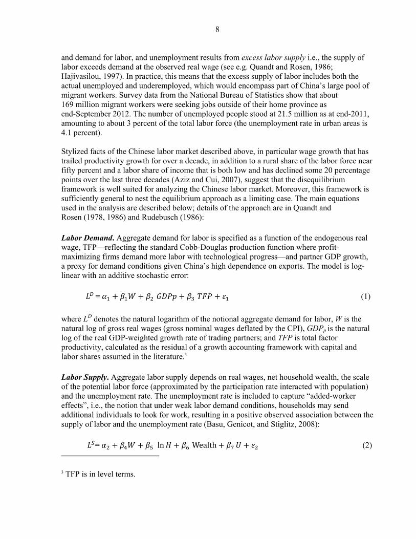
and demand for labor, and unemployment results from excess labor supply i.e., the supply of labor exceeds demand at the observed real wage (see e.g. Quandt and Rosen, 1986; Hajivasilou, 1997). In practice, this means that the excess supply of labor includes both the actual unemployed and underemployed, which would encompass part of China’s large pool of migrant workers. Survey data from the National Bureau of Statistics show that about 169 million migrant workers were seeking jobs outside of their home province as end-September 2012. The number of unemployed people stood at 21.5 million as at end-2011, amounting to about 3 percent of the total labor force (the unemployment rate in urban areas is 4.1 percent). Stylized facts of the Chinese labor market described above, in particular wage growth that has trailed productivity growth for over a decade, in addition to a rural share of the labor force near fifty percent and a labor share of income that is both low and has declined some 20 percentage points over the last three decades (Aziz and Cui, 2007), suggest that the disequilibrium framework is well suited for analyzing the Chinese labor market. Moreover, this framework is sufficiently general to nest the equilibrium approach as a limiting case. The main equations used in the analysis are described below; details of the approach are in Quandt and Rosen (1978, 1986) and Rudebusch (1986):

Labor Demand. Aggregate demand for labor is specified as a function of the endogenous real wage, TFP—reflecting the standard Cobb-Douglas production function where profit-maximizing firms demand more labor with technological progress—and partner GDP growth, a proxy for demand conditions given China’s high dependence on exports. The model is log-linear with an additive stochastic error:

 =          (1)

where LD denotes the natural logarithm of the notional aggregate demand for labor, W is the natural log of gross real wages (gross nominal wages deflated by the CPI), GDPp is the natural log of the real GDP-weighted growth rate of trading partners; and TFP is total factor productivity, calculated as the residual of a growth accounting framework with capital and labor shares assumed in the literature.3

Labor Supply. Aggregate labor supply depends on real wages, net household wealth, the scale of the potential labor force (approximated by the participation rate interacted with population) and the unemployment rate. The unemployment rate is included to capture “added-worker effects”, i.e., the notion that under weak labor demand conditions, households may send additional individuals to look for work, resulting in a positive observed association between the supply of labor and the unemployment rate (Basu, Genicot, and Stiglitz, 2008):

=     ln   Wealth   (2) 3 TFP is in level terms.

9

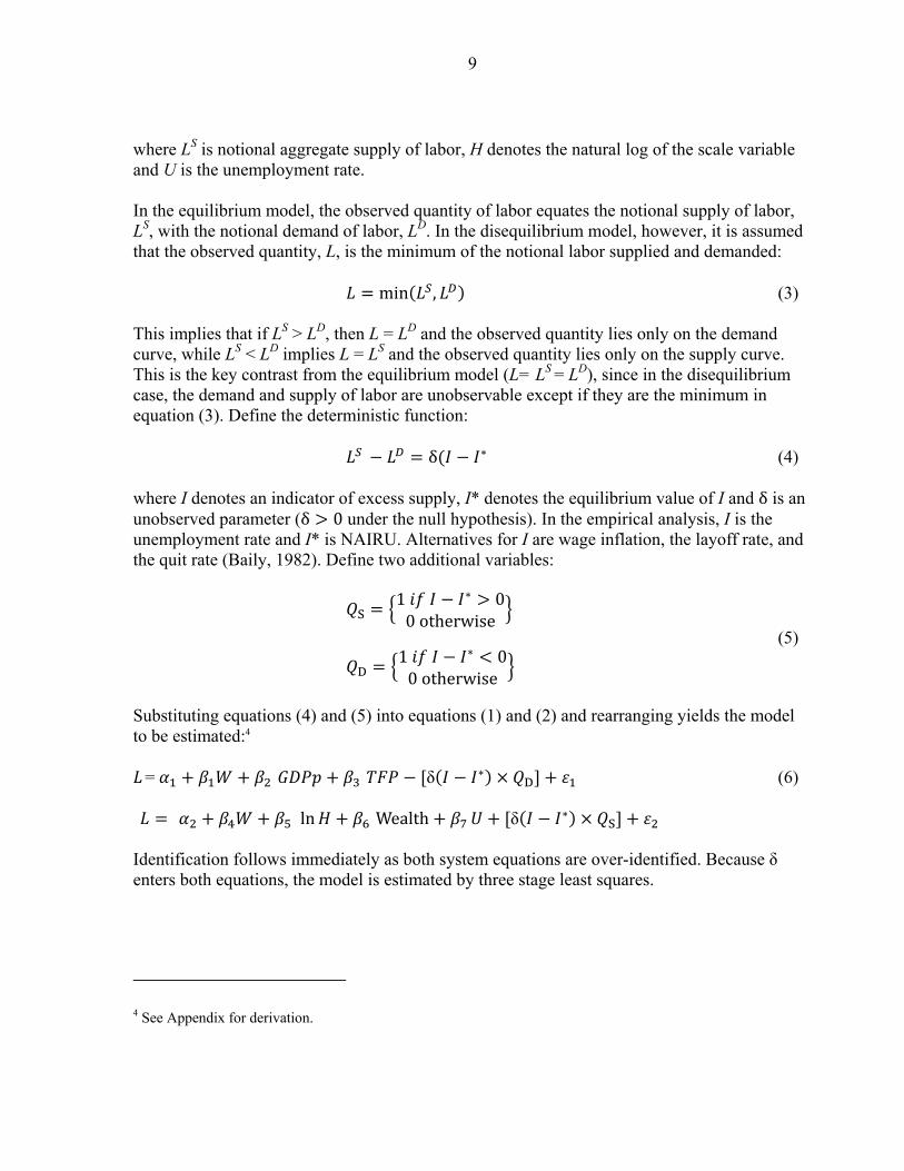
where LS is notional aggregate supply of labor, H denotes the natural log of the scale variable and U is the unemployment rate. In the equilibrium model, the observed quantity of labor equates the notional supply of labor, LS, with the notional demand of labor, LD. In the disequilibrium model, however, it is assumed that the observed quantity, L, is the minimum of the notional labor supplied and demanded:

min , (3) This implies that if LS > LD, then L = LD and the observed quantity lies only on the demand curve, while LS < LD implies L = LS and the observed quantity lies only on the supply curve. This is the key contrast from the equilibrium model (L= LS = LD), since in the disequilibrium case, the demand and supply of labor are unobservable except if they are the minimum in equation (3). Define the deterministic function:   δ (4) where I denotes an indicator of excess supply, I* denotes the equilibrium value of I and δ is an unobserved parameter (δ 0 under the null hypothesis). In the empirical analysis, I is the unemployment rate and I* is NAIRU. Alternatives for I are wage inflation, the layoff rate, and the quit rate (Baily, 1982). Define two additional variables:

S1    00 otherwise

(5)

D1    00 otherwise

Substituting equations (4) and (5) into equations (1) and (2) and rearranging yields the model to be estimated:4  =        δ D (6)

        ln   Wealth   δ S Identification follows immediately as both system equations are over-identified. Because δ enters both equations, the model is estimated by three stage least squares.

4 See Appendix for derivation.

10

IV. RESULTS

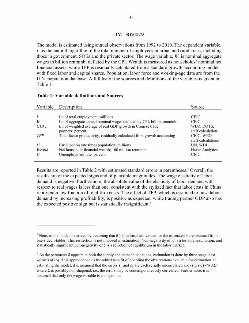
The model is estimated using annual observations from 1992 to 2010. The dependent variable, L, is the natural logarithm of the total number of employees in urban and rural areas, including those in government, SOEs and the private sector. The wage variable, W, is nominal aggregate wages in billion renminbi deflated by the CPI. Wealth is measured as households’ nominal net financial assets, while TFP is residually calculated from a standard growth accounting model with fixed labor and capital shares. Population, labor force and working-age data are from the U.N. population database. A full list of the sources and definitions of the variables is given in Table 1. Table 1: Variable definitions and Sources Variable Description Source L

Ln of total employment; millions

CEIC

W Ln of aggregate annual nominal wages deflated by CPI; billion renminbi CEIC GDPp Ln of weighted average of real GDP growth in Chinese trade

partners; percent WEO, DOTS, staff calculation

TFP Total factor productivity, residually calculated from growth accounting CEIC, WEO, staff calculations

H Participation rate times population; millions UN, WDI Wealth Net household financial wealth; 100 million renminbi Haver Analytics U Unemployment rate; percent CEIC

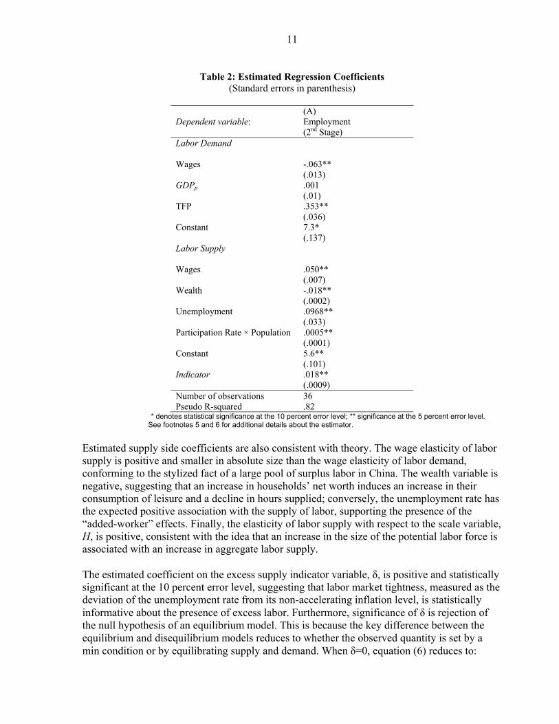
Results are reported in Table 2 with estimated standard errors in parentheses.5 Overall, the results are of the expected signs and of plausible magnitudes. The wage elasticity of labor demand is negative. Furthermore, the absolute value of the elasticity of labor demand with respect to real wages is less than one, consistent with the stylized fact that labor costs in China represent a low fraction of total firm costs. The effect of TFP, which is assumed to raise labor demand by increasing profitability, is positive as expected, while trading partner GDP also has the expected positive sign but is statistically insignificant.6

5 Note, as the model is derived by assuming that δ ≥ 0, critical test valued for the estimated δ are obtained from one-sided t-tables. This restriction is not imposed in estimation. Non-negativity of δ is a testable assumption, and statistically significant non-negativity of δ is a rejection of equilibrium in the labor market.

6 As the parameter δ appears in both the supply and demand equations, estimation is done by three stage least squares of (6). This approach yields the added benefit of doubling the observations available for estimation. In estimating the model, it is assumed that the errors and are each serially uncorrelated and ( , ~N(0,Σ) where Σ is possibly non-diagonal, i.e., the errors may be contemporaneously correlated. Furthermore, it is assumed that only the wage variable is endogenous.

11

Table 2: Estimated Regression Coefficients (Standard errors in parenthesis)

Dependent variable:

(A) Employment (2nd Stage)

Labor Demand

Wages -.063** (.013)

GDPp .001 (.01)

TFP .353** (.036)

Constant 7.3* (.137)

Labor Supply

Wages .050** (.007)

Wealth -.018** (.0002)

Unemployment .0968** (.033)

Participation Rate × Population .0005** (.0001)

Constant 5.6** (.101)

Indicator .018** (.0009)

Number of observations 36 Pseudo R-squared .82

* denotes statistical significance at the 10 percent error level; ** significance at the 5 percent error level. See footnotes 5 and 6 for additional details about the estimator.

Estimated supply side coefficients are also consistent with theory. The wage elasticity of labor supply is positive and smaller in absolute size than the wage elasticity of labor demand, conforming to the stylized fact of a large pool of surplus labor in China. The wealth variable is negative, suggesting that an increase in households’ net worth induces an increase in their consumption of leisure and a decline in hours supplied; conversely, the unemployment rate has the expected positive association with the supply of labor, supporting the presence of the “added-worker” effects. Finally, the elasticity of labor supply with respect to the scale variable, H, is positive, consistent with the idea that an increase in the size of the potential labor force is associated with an increase in aggregate labor supply. The estimated coefficient on the excess supply indicator variable, δ, is positive and statistically significant at the 10 percent error level, suggesting that labor market tightness, measured as the deviation of the unemployment rate from its non-accelerating inflation level, is statistically informative about the presence of excess labor. Furthermore, significance of δ is rejection of the null hypothesis of an equilibrium model. This is because the key difference between the equilibrium and disequilibrium models reduces to whether the observed quantity is set by a min condition or by equilibrating supply and demand. When δ=0, equation (6) reduces to:

12

 =         ɛ (7)

         ln   Wealth   ɛ

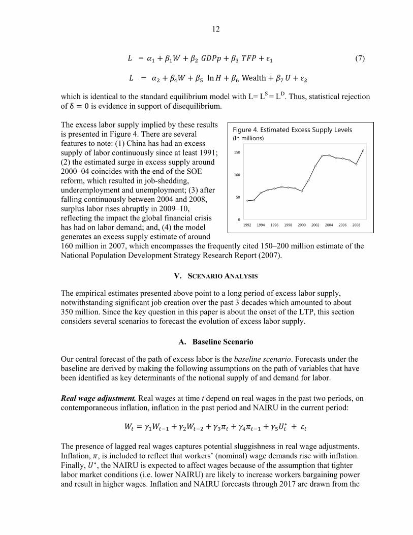
which is identical to the standard equilibrium model with L= LS = LD. Thus, statistical rejection of δ 0 is evidence in support of disequilibrium. The excess labor supply implied by these results is presented in Figure 4. There are several features to note: (1) China has had an excess supply of labor continuously since at least 1991; (2) the estimated surge in excess supply around 2000–04 coincides with the end of the SOE reform, which resulted in job-shedding, underemployment and unemployment; (3) after falling continuously between 2004 and 2008, surplus labor rises abruptly in 2009–10, reflecting the impact the global financial crisis has had on labor demand; and, (4) the model generates an excess supply estimate of around 160 million in 2007, which encompasses the frequently cited 150–200 million estimate of the National Population Development Strategy Research Report (2007).

V. SCENARIO ANALYSIS

The empirical estimates presented above point to a long period of excess labor supply, notwithstanding significant job creation over the past 3 decades which amounted to about 350 million. Since the key question in this paper is about the onset of the LTP, this section considers several scenarios to forecast the evolution of excess labor supply.

A. Baseline Scenario

Our central forecast of the path of excess labor is the baseline scenario. Forecasts under the baseline are derived by making the following assumptions on the path of variables that have been identified as key determinants of the notional supply of and demand for labor. Real wage adjustment. Real wages at time t depend on real wages in the past two periods, on contemporaneous inflation, inflation in the past period and NAIRU in the current period:

    The presence of lagged real wages captures potential sluggishness in real wage adjustments. Inflation, , is included to reflect that workers’ (nominal) wage demands rise with inflation. Finally, , the NAIRU is expected to affect wages because of the assumption that tighter labor market conditions (i.e. lower NAIRU) are likely to increase workers bargaining power and result in higher wages. Inflation and NAIRU forecasts through 2017 are drawn from the

Figure 4. Estimated Excess Supply Levels (In millions)

0

50

100

150

1992 1994 1996 1998 2000 2002 2004 2006 2008

13

IMF World Economic Outlook (WEO), and both variables are assumed to grow at the 2017 rate thereafter. Household net wealth. The evolution of net financial wealth (NFW) is derived from a standard wealth accumulation equation where net wealth increase each period due to interest payments on the stock, and the new flow from household saving:

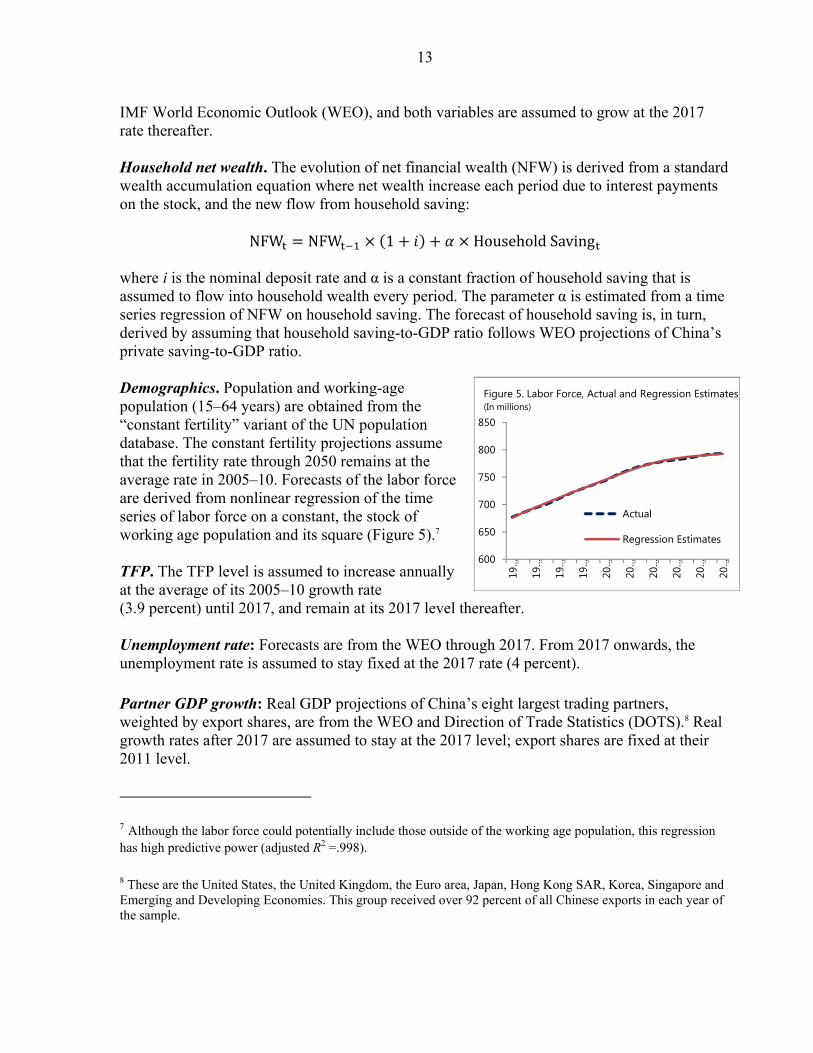
NFW NFW 1 Household Saving where i is the nominal deposit rate and α is a constant fraction of household saving that is assumed to flow into household wealth every period. The parameter α is estimated from a time series regression of NFW on household saving. The forecast of household saving is, in turn, derived by assuming that household saving-to-GDP ratio follows WEO projections of China’s private saving-to-GDP ratio. Demographics. Population and working-age population (15–64 years) are obtained from the “constant fertility” variant of the UN population database. The constant fertility projections assume that the fertility rate through 2050 remains at the average rate in 2005–10. Forecasts of the labor force are derived from nonlinear regression of the time series of labor force on a constant, the stock of working age population and its square (Figure 5).7 TFP. The TFP level is assumed to increase annually at the average of its 2005–10 growth rate (3.9 percent) until 2017, and remain at its 2017 level thereafter. Unemployment rate: Forecasts are from the WEO through 2017. From 2017 onwards, the unemployment rate is assumed to stay fixed at the 2017 rate (4 percent). Partner GDP growth: Real GDP projections of China’s eight largest trading partners, weighted by export shares, are from the WEO and Direction of Trade Statistics (DOTS).8 Real growth rates after 2017 are assumed to stay at the 2017 level; export shares are fixed at their 2011 level. 7 Although the labor force could potentially include those outside of the working age population, this regression has high predictive power (adjusted R2 =.998).

8 These are the United States, the United Kingdom, the Euro area, Japan, Hong Kong SAR, Korea, Singapore and Emerging and Developing Economies. This group received over 92 percent of all Chinese exports in each year of the sample.

600

650

700

750

800

850

19…

19…

19…

19…

20…

20…

20…

20…

20…

20…

Actual

Regression Estimates

Figure 5. Labor Force, Actual and Regression Estimates (In millions)

14

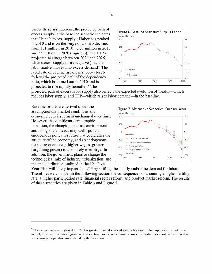
Under these assumptions, the projected path of excess supply in the baseline scenario indicates that China’s excess supply of labor has peaked in 2010 and is on the verge of a sharp decline: from 151 million in 2010, to 57 million in 2015, and 33 million in 2020 (Figure 6). The LTP is projected to emerge between 2020 and 2025, when excess supply turns negative (i.e., the labor market moves into excess demand). The rapid rate of decline in excess supply closely follows the projected path of the dependency ratio, which bottomed out in 2010 and is projected to rise rapidly hereafter. 9 The projected path of excess labor supply also reflects the expected evolution of wealth—which reduces labor supply, and TFP—which raises labor demand—in the baseline. Baseline results are derived under the assumption that market conditions and economic policies remain unchanged over time. However, the significant demographic transition, the changing external environment and rising social needs may well spur an endogenous policy response that could alter the structure of the economy, and an endogenous market response (e.g. higher wages, greater bargaining power) is also likely to emerge. In addition, the government plans to change the technological mix of industry, urbanization, and income distribution outlined in the 12th Five-Year Plan will likely impact the LTP by shifting the supply and/or the demand for labor. Therefore, we consider in the following section the consequences of assuming a higher fertility rate, a higher participation rate, financial sector reform, and product market reform. The results of these scenarios are given in Table 3 and Figure 7.

9 The dependency ratio (less than 15 plus greater than 64 years of age, in fraction of the population) is not in the model; however, the working-age ratio is captured in the scale variable since the participation rate is measured as working-age population normalized by the labor force.

Figure 6. Baseline Scenario: Surplus Labor (In millions)

-300

-200

-100

0

100

200

-300

-200

-100

0

100

200

1992 2002 2012 2022

Actual

Baseline

2030

Figure 7. Alternative Scenarios: Surplus Labor (In millions)

-300

-200

-100

0

100

200

-300

-200

-100

0

100

200

1992 2002 2012 2022

Actual

1. High Fertility Scenario

2. Higher Participation Rate

3. Financial Reform

4. Product Market Reform

Baseline

2030

( )

15

B. Increase in the Fertility Rate

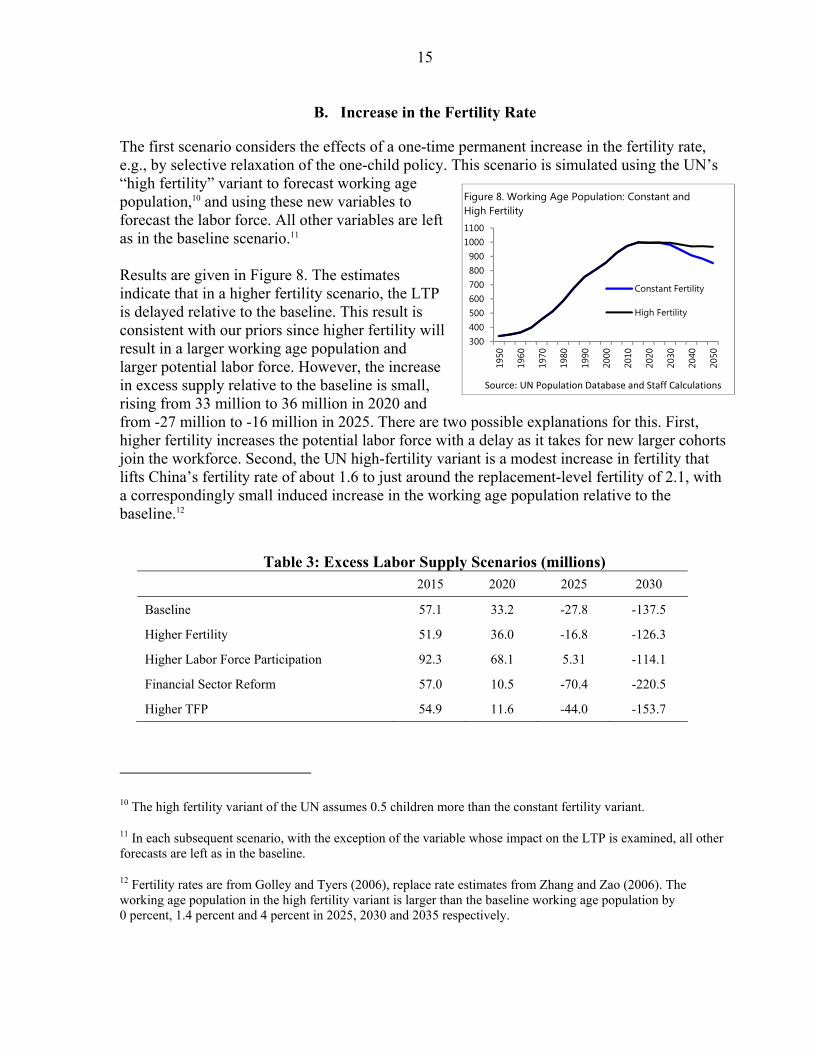
The first scenario considers the effects of a one-time permanent increase in the fertility rate, e.g., by selective relaxation of the one-child policy. This scenario is simulated using the UN’s “high fertility” variant to forecast working age population,10 and using these new variables to forecast the labor force. All other variables are left as in the baseline scenario.11 Results are given in Figure 8. The estimates indicate that in a higher fertility scenario, the LTP is delayed relative to the baseline. This result is consistent with our priors since higher fertility will result in a larger working age population and larger potential labor force. However, the increase in excess supply relative to the baseline is small, rising from 33 million to 36 million in 2020 and from -27 million to -16 million in 2025. There are two possible explanations for this. First, higher fertility increases the potential labor force with a delay as it takes for new larger cohorts join the workforce. Second, the UN high-fertility variant is a modest increase in fertility that lifts China’s fertility rate of about 1.6 to just around the replacement-level fertility of 2.1, with a correspondingly small induced increase in the working age population relative to the baseline.12

Table 3: Excess Labor Supply Scenarios (millions) 2015 2020 2025 2030

Baseline 57.1 33.2 -27.8 -137.5

Higher Fertility 51.9 36.0 -16.8 -126.3

Higher Labor Force Participation 92.3 68.1 5.31 -114.1

Financial Sector Reform 57.0 10.5 -70.4 -220.5

Higher TFP 54.9 11.6 -44.0 -153.7

10 The high fertility variant of the UN assumes 0.5 children more than the constant fertility variant.

11 In each subsequent scenario, with the exception of the variable whose impact on the LTP is examined, all other forecasts are left as in the baseline.

12 Fertility rates are from Golley and Tyers (2006), replace rate estimates from Zhang and Zao (2006). The working age population in the high fertility variant is larger than the baseline working age population by 0 percent, 1.4 percent and 4 percent in 2025, 2030 and 2035 respectively.

300400500600700800900

10001100

1950

1960

1970

1980

1990

2000

2010

2020

2030

2040

2050

Constant Fertility

High Fertility

Figure 8. Working Age Population: Constant andHigh Fertility

Source: UN Population Database and Staff Calculations

16

C. Higher Labor Force Participation Rates

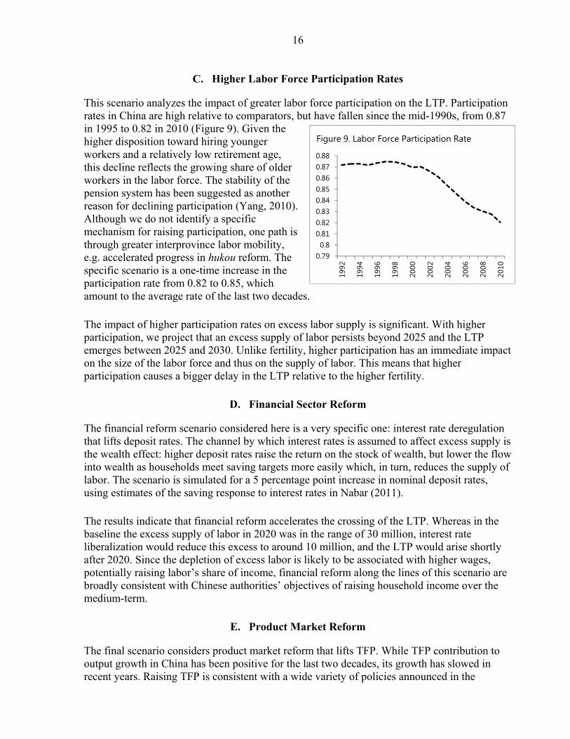
This scenario analyzes the impact of greater labor force participation on the LTP. Participation rates in China are high relative to comparators, but have fallen since the mid-1990s, from 0.87 in 1995 to 0.82 in 2010 (Figure 9). Given the higher disposition toward hiring younger workers and a relatively low retirement age, this decline reflects the growing share of older workers in the labor force. The stability of the pension system has been suggested as another reason for declining participation (Yang, 2010). Although we do not identify a specific mechanism for raising participation, one path is through greater interprovince labor mobility, e.g. accelerated progress in hukou reform. The specific scenario is a one-time increase in the participation rate from 0.82 to 0.85, which amount to the average rate of the last two decades. The impact of higher participation rates on excess labor supply is significant. With higher participation, we project that an excess supply of labor persists beyond 2025 and the LTP emerges between 2025 and 2030. Unlike fertility, higher participation has an immediate impact on the size of the labor force and thus on the supply of labor. This means that higher participation causes a bigger delay in the LTP relative to the higher fertility.

D. Financial Sector Reform

The financial reform scenario considered here is a very specific one: interest rate deregulation that lifts deposit rates. The channel by which interest rates is assumed to affect excess supply is the wealth effect: higher deposit rates raise the return on the stock of wealth, but lower the flow into wealth as households meet saving targets more easily which, in turn, reduces the supply of labor. The scenario is simulated for a 5 percentage point increase in nominal deposit rates, using estimates of the saving response to interest rates in Nabar (2011). The results indicate that financial reform accelerates the crossing of the LTP. Whereas in the baseline the excess supply of labor in 2020 was in the range of 30 million, interest rate liberalization would reduce this excess to around 10 million, and the LTP would arise shortly after 2020. Since the depletion of excess labor is likely to be associated with higher wages, potentially raising labor’s share of income, financial reform along the lines of this scenario are broadly consistent with Chinese authorities’ objectives of raising household income over the medium-term.

E. Product Market Reform

The final scenario considers product market reform that lifts TFP. While TFP contribution to output growth in China has been positive for the last two decades, its growth has slowed in recent years. Raising TFP is consistent with a wide variety of policies announced in the

0.790.8

0.810.820.830.840.850.860.870.88

1992

1994

1996

1998

2000

2002

2004

2006

2008

2010

Figure 9. Labor Force Participation Rate

17

12th Five-Year Plan, such as greater competition in the service sector and investment in higher value-added activities. Unlike the other scenarios, higher TFP work through the labor demand side in our framework, raising firm profitability and thus the demand for labor (Freeman, 1980). This scenario is simulated through a one-time permanent increase in the growth rate of TFP to 4.5 percent, the average TFP growth in the last two decades. The impact on the LTP from higher TFP is qualitatively similar to financial reform: a faster decline of excess labor supply, and a faster emergence of the LTP, relative to the baseline. However, this result is, in part, a consequence of the model specification where TFP does not directly affect the supply of labor. In an alternative setup (e.g. Pissarides and Valenti, 2007), where gains in productivity translate into lower unemployment—and thus a lower notional supply of labor—a smaller decrease in excess labor supply could result.

VI. CONCLUSION

China is on the eve of a demographic shift that will have profound consequences on its economic and social landscape. Within a few years the working age population will reach a historical peak, and will then begin a precipitous decline. The core of the working age population, those aged 20–39 years, has already begun to shrink. With this, the vast supply of low-cost workers—a core engine of China’s growth model—will dissipate, with potentially far-reaching implications domestically and externally. This paper empirically assessed when labor shortages might. Our central result is that, barring an endogenous market or policy response, the excess supply of labor—the reserve of unemployed and underemployed workers (which is currently in the range of 150 million)—will fall to about 30 million by 2020 and the LTP will be crossed between 2020 and 2025. An endogenous policy response to potential labor shortages is, however, likely as the government tries to slow the transition to the LTP. Market mechanisms that result in higher wages as labor markets tighten, or induce a transition to more capital-intensive production, may also offset the shrinking labor pool. Scenario analysis reveals that higher fertility through relaxation of the one-child policy and greater labor force participation through hukou reform will delay depletion of excess labor. Financial reform and higher TFP, on the other hand, accelerate the transition to a labor shortage economy, through wealth effects and greater profitability of firms, respectively. Quantitative estimates of the excess supply of labor and the timing of the LTP presented in this paper are inherently uncertain. In addition, alternative scenario exercises are analyzed for specific reforms of particular magnitudes and do not take into account potential inter-scenario effects (e.g., the offsetting impacts of higher fertility and financial sector reform). That said, the main takeaway of the analysis is that market and policy responses to the declining surplus labor will be largely peripheral, as demographics forces play a dominant role in the imminent transition to a labor shortage economy.

18

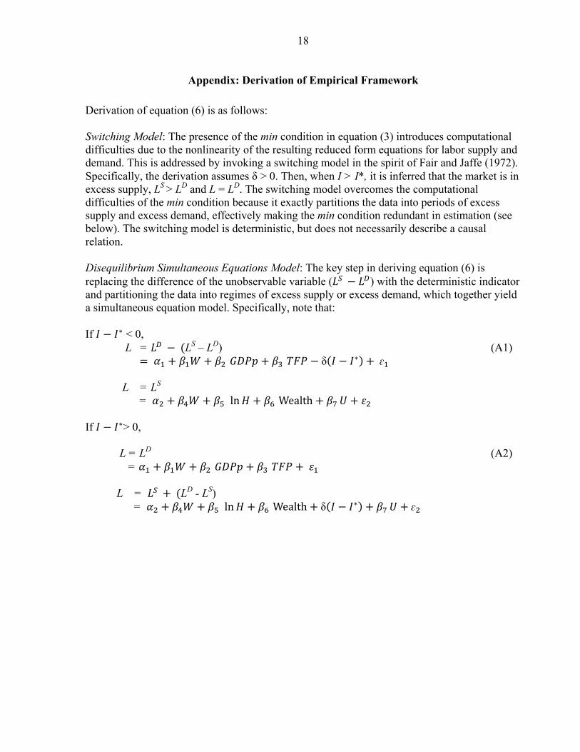
Appendix: Derivation of Empirical Framework Derivation of equation (6) is as follows: Switching Model: The presence of the min condition in equation (3) introduces computational difficulties due to the nonlinearity of the resulting reduced form equations for labor supply and demand. This is addressed by invoking a switching model in the spirit of Fair and Jaffe (1972). Specifically, the derivation assumes δ > 0. Then, when I > I*, it is inferred that the market is in excess supply, LS > LD and L = LD. The switching model overcomes the computational difficulties of the min condition because it exactly partitions the data into periods of excess supply and excess demand, effectively making the min condition redundant in estimation (see below). The switching model is deterministic, but does not necessarily describe a causal relation. Disequilibrium Simultaneous Equations Model: The key step in deriving equation (6) is replacing the difference of the unobservable variable (   ) with the deterministic indicator and partitioning the data into regimes of excess supply or excess demand, which together yield a simultaneous equation model. Specifically, note that: If < 0, L =     LS – LD) (A1)         δ  ɛ    L = LS

=      ln   Wealth   If > 0, L = LD (A2)

=            L =       LD - LS) =      ln   Wealth δ   ɛ

19

REFERENCES

Ahuja, A., N. Chalk, M. Nabar, P. N’Diaye, and N. Porter, 2012, “An End to China’s

Imbalances?” IMF Working Paper 12/100 (Washington: International Monetary Fund).

Aziz, J., and L. Cui, 2007, “Explaining China’s Low Consumption: The Neglected Role of Household Income,” IMF Working Paper 7/181 (Washington: International Monetary Fund).

Baily, M., 1982, Workers, Jobs and Inflation (Washington, DC: The Brookings Institution).

Barro, R.J., and H.I. Grossman, 1971, “A General Disequilibrium Model of Income and Employment,” The American Economic Review, Vol. 61 (1), pp. 82–93.

Basu, K., J. E. Stiglitz, and G. Genicot, 2008, Unemployment and Wage Rigidity When Labor Supply is a Household Decision (New York: Cornell University).

Cai, F., and M. Wang, 2008, “A Counterfactual of Unlimited Surplus Labour in Rural China,” China and the World Economy, 16, pp. 51–65.

Chan, K. W., 2010, “A China Paradox: Migrant Labor Shortage amidst Rural Labor Supply Abundance,” Eurasian Geography and Economics, 51, pp. 513–30.

Fair, R., and A. Jaffe, 1972, “Methods of Estimation for Markets in Disequilibrium,” Econometrica, 40, 497–514.

Freeman, R., 1980, “The Evolution of the American Labor Market, 1948-80” in The American Economy in Transition, ed. by Feldstein (Chicago: University of Chicago Press).

Garnaut, R., 2006, “The Turning Point in China’s Economic Development,” in The Turning Point in China’s Economic Development, ed. by Garnaut and Song (Canberra: Asia Pacific Press).

Golley, J., and R. Tyers, 2006, “China’s Growth to 2030: Demographic Change and the Labour Supply Constraint,” Australian National University Working Paper.

Hajivasilou, V., 1997, “Macroeconomic Shocks in an Aggregative Disequilibrium Model,” mimeo, London School of Economics.

International Monetary Fund, 2011, People’s Republic of China: Spillover Report for the 2011 Article IV Consultation and Selected Issues. Available via internet: www.imf.org/external/pubs/ft/scr/2011/cr11193.pdf.

Knight, J., Q. Deng, and S. Li, 2011, “The Puzzle of Migrant Labour Shortage and Rural Labour Surplus in China,” 22, pp. 585–600.

Kwan, C.H., 2007, “China Shifts from Labor Surplus to Labor Shortage: Challenges and Opportunities in a New Stage of Development,” RIETI.

20

Lewis, W. A., 1954. “Economic Development with Unlimited Supplies of Labour,” The Manchester School, 22, pp. 139–92.

Lucas, R.E., and L. Rapping, 1969, “Real Wages, Employment, and Inflation,” The Journal of Political Economy, 77, 721–54.

Nabar, M., 2011, “Targets, Interest Rates and Household Saving in Urban China,” IMF Working Papers, 11/223 (Washington: International Monetary Fund).

National Development Strategy Research Report, 2007. Available via internet: http://www.chinapop.gov.cn/gxdd/t20070111_172058513.html

Pissarides, M., and G. Valenti, 2007, “The Impact of TFP Growth on Steady-State Unemployment,” International Economic Review, 48, 607–40.

Quandt, R.E., and H. Rosen, 1978, “Estimation of a Disequilibrium Aggregate Labor Market,” Review of Economics and Statistics, XL, 371–79.

Quandt, R.E., and H. Rosen, 1986, “Unemployment, Disequilibrium and the Short Run Phillips Curve,” Journal of Applied Econometrics, 1, 3, 235–53.

Rudebusch, G.D., 1986, “Testing for Labor Market Equilibrium with an Exact Excess Demand Disequilibrium Model,” The Review of Economics and Statistics, 68, 468–76.

Yang, D.U., and M. Wang, 2010, “Demographic aging and employment in China,” Institute of Population and Labour Economics, Chinese Academy of Social Sciences.

Zhang, G., and Z. Zhao, 2006, “Reexamining China’s Fertility Puzzle: Data Collection and Quality over the Last Two Decades,” Population and Development Review, 32, 293–321.

Zhang, X, J. Yang, and S. Wang, 2010, “China has reached the Lewis Turning Point,” IFPRI Working Paper.