Embed Size (px)
Citation preview
Deep Learning for Anomaly Detection: A Review
GUANSONG PANG∗, University of AdelaideCHUNHUA SHEN, University of AdelaideLONGBING CAO, University of Technology SydneyANTON VAN DEN HENGEL, University of Adelaide
Anomaly detection, a.k.a. outlier detection, has been a lasting yet active research area in various researchcommunities for several decades. There are still some unique problem complexities and challenges thatrequire advanced approaches. In recent years, deep learning enabled anomaly detection, i.e., deep anomalydetection, has emerged as a critical direction. This paper reviews the research of deep anomaly detection witha comprehensive taxonomy of detection methods, covering advancements in three high-level categories and11 fine-grained categories of the methods. We review their key intuitions, objective functions, underlyingassumptions, advantages and disadvantages, and discuss how they address the aforementioned challenges. Wefurther discuss a set of possible future opportunities and new perspectives on addressing the challenges.
CCS Concepts: • Computing methodologies→ Anomaly detection; Neural networks.
Additional Key Words and Phrases: anomaly detection, deep learning, outlier detection, neural networks
1 INTRODUCTIONAnomaly detection, a.k.a. outlier detection, is referred to as the process of detecting data instancesthat significantly deviate from the majority of data instances. Anomaly detection has been an activeresearch area for several decades, with early exploration dating back as far as to 1960s [53]. Due tothe increasing demand and broader applications in domains such as risk management, compliance,security, financial surveillance, health and medical risk, and AI safety, anomaly detection playsincreasingly important roles, highlighted in various communities including data mining, machinelearning, computer vision and statistics. In recent years, deep learning has shown tremendouscapabilities in learning expressive representations of complex data such as high-dimensional data,temporal data, spatial data and graph data, pushing the boundaries of different learning tasks.Deep learning for anomaly detection, deep anomaly detection for short, aim at learning featurerepresentations or anomaly scores via neural networks for the sake of anomaly detection. In recentyears, a large number of deep anomaly detection methods have been introduced, demonstratingsignificantly better performance than conventional anomaly detection on addressing challenging de-tection problems in a variety of real-world applications. This work aims to provide a comprehensivereview of this area. We first discuss the problem nature and major challenges of anomaly detection,then systematically review the current deep anomaly detection methods and their capabilities inaddressing these challenges, and finally presents a number of future opportunities in this area.As a popular area, a number of studies [2, 4, 16, 28, 54, 63, 178] have been dedicated to the
categorization and review of anomaly detection techniques. However, they all focus on conventionalanomaly detection methods only. One work closely related to ours is [26]. It presents a goodsummary of a number of real-world applications of deep anomaly detection, but only providessome very high-level outlines of selective categories of the techniques, from which it is highly∗Corresponding author, email: [email protected]
Authors’ addresses: Guansong Pang, University of Adelaide, Adelaide, South Australia, 5005; Chunhua Shen, University ofAdelaide, Adelaide, South Australia, 5005; Longbing Cao, University of Technology Sydney, Sydney, New South Wales,2007; Anton van den Hengel, University of Adelaide, Adelaide, South Australia, 5005.
202x. 0360-0300/202x/7-ART $15.00https://doi.org/10.1145/nnnnnnn.nnnnnnn
ACM Comput. Surv., Vol. xx, No. x, Article . Publication date: July 202x.
arX
iv:2
007.
0250
0v2
[cs
.LG
] 8
Jul
202
0
2 Pang, et al.
difficult, if not impossible, to gain the sense of the approaches taken by the current methods andthe intuition behind the methods. By contrast, to answer why we need deep anomaly detection,this review delineates the formulation of current deep detection methods to gain key insightsabout their underlying intuitions, inherent capabilities and weakness on addressing some largelyunsolved challenges in anomaly detection. This forms a deep understanding of the problem natureand the state-of-the-art, and brings about genuine open opportunities.
In summary, this work makes the following five major contributions:• Problem nature and challenges. We discuss some unique problem complexities underlyinganomaly detection and the resulting largely unsolved challenges.
• Categorization and formulation. We formulate the current deep anomaly detection methodsinto three principled frameworks: deep learning for generic feature extraction, learning rep-resentations of normality, and end-to-end anomaly score learning. A hierarchical taxonomyis presented to categorize the methods based on 11 different modeling perspectives.
• Comprehensive literature review. We review a large number of relevant studies in leadingconferences and journals of several relevant communities, including machine learning, datamining, computer vision and artificial intelligence, to present a comprehensive literaturereview of the research progress. To provide an in-depth introduction, we delineate the basicassumptions, objective functions, key intuitions and their capabilities in addressing some ofthe aforementioned challenges by all categories of the methods.
• Future opportunities. We further discuss a set of possible future opportunities and theirimplication to addressing relevant challenges.
• Source codes and datasets. We solicit a collection of publicly accessible source codes of nearlyall categories of methods and a large number of real-world datasets with real anomalies tooffer some empirical comparison benchmarks.
2 ANOMALY DETECTION: PROBLEM COMPLEXITIES AND CHALLENGESOwing to the unique nature, anomaly detection presents distinct problem complexities from themajority of analytical and learning problems and tasks. This section summarizes such intrinsiccomplexities and unsolved detection challenges in complex anomaly data.
2.1 Major Problem ComplexitiesUnlike those problems and tasks on majority, regular or evident patterns, anomaly detectionaddresses minority, unpredictable/uncertain and rare events, leading to some unique complexitiesbelow that render general deep learning techniques ineffective.
• Unknownness. Anomalies are associated with many unknowns, e.g., instances with un-known abrupt behaviors, data structures, and distributions. They remain unknown untilactually occur, such as novel terrorist attacks, frauds and network intrusions.
• Heterogeneous anomaly classes. Anomalies are irregular, and thus, one class of anom-alies may demonstrate completely different abnormal characteristics from another class ofanomalies. For example, in video surveillance, the abnormal events robbery, traffic accidentsand burglary are visually highly different.
• Rarity and class imbalance. Anomalies are typically rare data instances, contrasting tonormal instances that often account for an overwhelming proportion of the data. Therefore,it is difficult, if not impossible, to collect a large amount of labeled abnormal instances.This results in the unavailability of large-scale labeled data in most applications. The classimbalance is also due to the fact that misclassification of anomalies is normally much morecostly than that of normal instances.
ACM Comput. Surv., Vol. xx, No. x, Article . Publication date: July 202x.
Deep Learning for Anomaly Detection: A Review 3
• Diverse types of anomaly. Three completely different types of anomaly have been explored[28]. Point anomalies are individual instances that are anomalous w.r.t. the majority ofother individual instances, e.g., the abnormal health indicators of a patient. Conditionalanomalies, a.k.a. contextual anomalies, also refer to individual anomalous instances but in aspecific context, i.e., data instances are anomalous in the specific context, otherwise normal.The contexts can be highly different in real-world applications, e.g., sudden temperaturedrop/increase in a particular temporal context, or rapid credit card transactions in unusualspatial contexts. Group anomalies, a.k.a. collective anomalies, are a subset of data instancesanomalous as a whole w.r.t. the other data instances; the individual members of the collectiveanomaly may not be anomalies, e.g., exceptionally dense subgraphs formed by fake accountsin social network are anomalies as a collection, but the individual nodes in those subgraphscan be as normal as real accounts.
2.2 Main Detection ChallengesThe above complex problem nature leads to a number of detection challenges to traditional anomalydetection methods and widely-used general deep learning methods. Some challenges, such asscalability w.r.t. data size, have been well addressed in recent years, while the following are largelyunsolved, to which deep anomaly detection can play some essential roles.
• CH1: Low anomaly detection recall rate. Since anomalies are highly rare and heteroge-neous, it is difficult to identify all of the anomalies. Many normal instances are wronglyreported as anomalies while true yet sophisticated anomalies are missed. Although a plethoraof anomaly detection methods have been introduced over the years, the current state-of-the-art methods, especially unsupervised methods (e.g., [17, 85]), still often incur high falsepositives on real-world datasets [20, 116]. How to reduce false positives and enhance detec-tion recall rates is one of the most important and yet difficult challenges, particularly for thesignificant expense of failing to spotting anomalies.
• CH2: Anomaly detection in high-dimensional and/or not-independent data. Anom-alies often exhibit evident abnormal characteristics in a low-dimensional space yet becomehidden and unnoticeable in a high-dimensional space. High-dimensional anomaly detec-tion has been a long-standing problem [178]. Performing anomaly detection in a reducedlower-dimensional space spanned by a small subset of original features or newly constructedfeatures is a straightforward solution, e.g., in subspace-based [71, 78, 86, 124] and featureselection-based methods [12, 111, 113, 113]. However, identifying intricate (e.g., high-order,nonlinear and heterogeneous) feature interactions and couplings [22] may be essential inhigh-dimensional data yet remains a major challenge for anomaly detection. Further, how toguarantee the new feature space preserved proper information for specific detection meth-ods is critical to downstream accurate anomaly detection, but it is challenging due to theaforementioned unknowns and heterogeneities of anomalies. Also, it is challenging to detectanomalies from instances that may be dependent on each other such as by temporal, spatial,graph-based and other interdependency relationships [2, 4, 22, 54].
• CH3: Data-efficient learning of normality/abnormality. Due to the difficulty and costof collecting large-scale labeled anomaly data, fully supervised anomaly detection is often im-practical as it assumes the availability of labeled training data with both normal and anomalyclasses. In the last decade, major research efforts have been focused on unsupervised anomalydetection that does not require any labeled training data. However, unsupervised methods donot have any prior knowledge of true anomalies. They rely heavily on their assumption onthe distribution of anomalies but fail to work in datasets where their assumption is violated.
ACM Comput. Surv., Vol. xx, No. x, Article . Publication date: July 202x.
4 Pang, et al.
On the other hand, it is often not difficult to collect labeled normal data and some labeledanomaly data. In practice, it is often suggested to leverage such readily accessible labeled dataas much as possible [2]. Thus, utilizing those labeled data to learn expressive representationsof normality/abnormality is crucial for accurate anomaly detection. Semi-supervised anomalydetection, which assumes that there exists a set of labeled training data1, is a research directiondedicated to this problem. Another research line is weakly-supervised anomaly detection thatassumes we have some labels for anomaly classes yet the class labels are partial/incomplete(i.e., they do not span the entire set of anomaly class), inexact (i.e., coarse-grained labels), orinaccurate (i.e., some given labels can be incorrect). Two major challenges are how to learnexpressive normality/abnormality representations with a small amount of labeled anomalydata and how to learn detection models that are generalized to novel anomalies uncoveredby the given labeled anomaly data.
• CH4: Noise-resilient anomaly detection. Many weakly/semi-supervised anomaly detec-tion methods assume the given labeled training data is clean, which can be highly vulnerableto noisy instances that are mistakenly labeled as an opposite class label. In such cases, wemay use unsupervised methods instead, but this fails to utilize the genuine labeled data.Additionally, there often exists large-scale anomaly-contaminated unlabeled data. Noise-resilient models can further leverage those unlabeled data for more accurate detection. Themain challenge is that the amount of noises can differ significantly from datasets and noisyinstances may be irregularly distributed in the data space.
• CH5: Detection of complex anomalies. Most of existing methods are for point anomalies,which cannot be used for conditional anomaly and group anomaly since they exhibit com-pletely different behaviors from point anomalies. One main challenge here is to incorporatethe concept of conditional/group anomalies into anomaly measures/models. Also, currentmethods mainly focus on detect anomalies from single data sources, while many applicationsrequire the detection of anomalies with multiple heterogeneous data sources, e.g., multidi-mensional data, graph, image, text and audio data. One main challenge is that some anomaliescan be detected only when considering two or more data sources.
• CH6: Anomaly explanation. In many critical domains there may be some major risks ifanomaly detection models are directly used as black-box models. For example, the rare datainstances reported as anomalies may lead to possible algorithmic bias against the minoritygroups presented in the data, such as under-represented groups in fraud detection and crimedetection systems. An effective approach to mitigate this type of risk is to have anomalyexplanation algorithms that provide straightforward clues about why a specific data instanceis identified as anomaly. Providing such explanation can be as important as detection accuracyin some applications. However, most existing anomaly detection studies focus on devisingaccurate detection models only, ignoring the capability of providing explanation of theidentified anomalies. To derive anomaly explanation from specific detection methods is still alargely unsolved problem, especially for complex models. Developing inherently interpretableanomaly detection models is also crucial, but it remains a main challenge to well balance themodel’s interpretability and effectiveness.
1There have been some studies that refer the methods trained with purely normal training data to be unsupervised approach.However, this setting is different from the general sense of an unsupervised setting. To avoid unnecessary confusion,following [2, 28], these methods are referred to as semi-supervised methods hereafter.
ACM Comput. Surv., Vol. xx, No. x, Article . Publication date: July 202x.
Deep Learning for Anomaly Detection: A Review 5
3 ADDRESSING THE CHALLENGES WITH DEEP ANOMALY DETECTION3.1 PreliminariesDeep neural networks leverage complex compositions of linear/non-linear functions that can berepresented by a computational graph to learn expressive representations [50]. Two basic buildingblocks of deep learning are activation functions and layers. Activation functions determine theoutput of computational graph nodes (i.e., neurons in neural networks) given some inputs. Theycan be linear or non-linear functions. Some popular activation functions include linear, sigmoid,tanh, ReLU (Rectified Linear Unit) and its variants. A layer in neural networks refers to a set ofneurons stacked in some forms. Commonly-used layers include fully connected, convolutional& pooling, and recurrent layers. These layers can be leveraged to build different popular neuralnetworks. For example, multilayer perceptron (MLP) networks are composed by fully connectedlayers, convolutional neural networks (CNN) are featured by varying groups of convolutional& pooling layers, and recurrent neural networks (RNN), e.g., vanilla RNN, gated recurrent units(GRU) and long short term memory (LSTM), are built upon recurrent layers. See [50] for detailedintroduction of these neural networks.Given a dataset X = {x1, x2, · · · , xN } with xi ∈ RD , let Z ∈ RK (K ≪ N ) be a representation
space, then deep anomaly detection aims at learning a feature representation mapping functionϕ(·) : X 7→ Z or an anomaly score learning function τ (·) : X 7→ R in a way that anomalies can beeasily differentiated from the normal data instances in the ϕ or τ space, where both ϕ and τ are aneural network-enabled mapping function with H ∈ N hidden layers and their weight matricesΘ = {M1,M2, · · · ,MH }. In the case of learning the feature mapping ϕ(·), an additional step isrequired to calculate the anomaly score of each data instance in the new representation space,while τ (·) can directly infer the anomaly scores with raw data inputs.
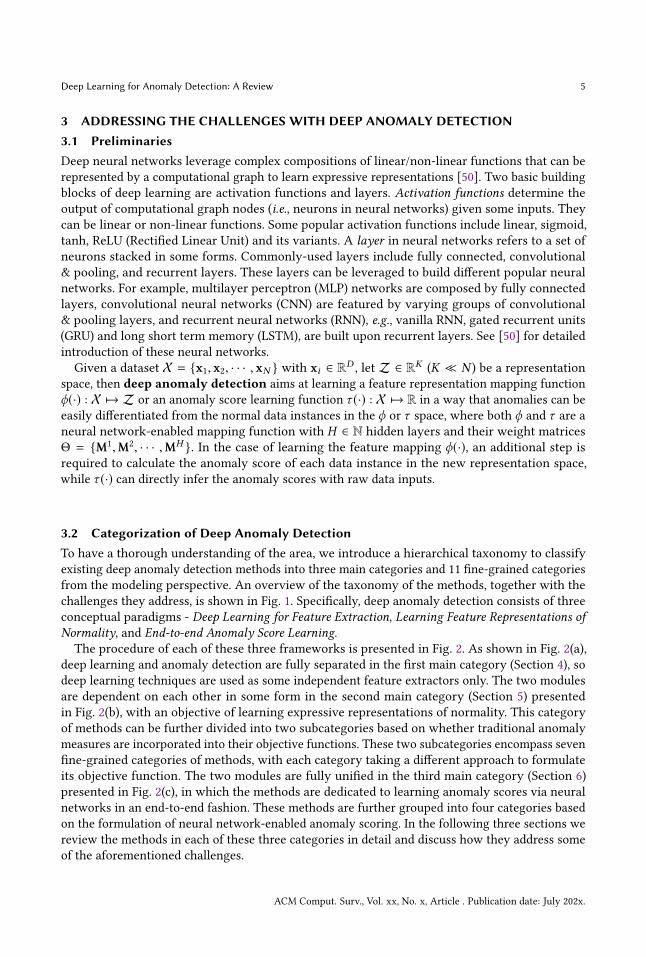
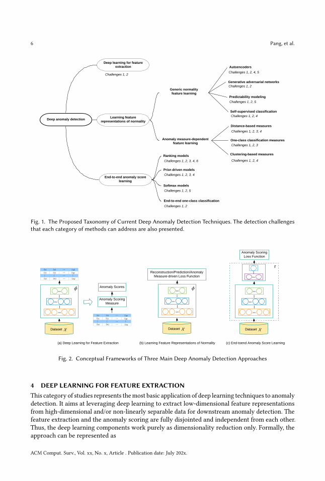
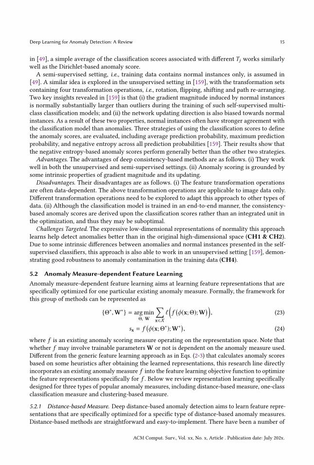
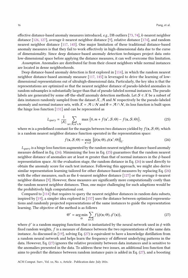
3.2 Categorization of Deep Anomaly DetectionTo have a thorough understanding of the area, we introduce a hierarchical taxonomy to classifyexisting deep anomaly detection methods into three main categories and 11 fine-grained categoriesfrom the modeling perspective. An overview of the taxonomy of the methods, together with thechallenges they address, is shown in Fig. 1. Specifically, deep anomaly detection consists of threeconceptual paradigms - Deep Learning for Feature Extraction, Learning Feature Representations ofNormality, and End-to-end Anomaly Score Learning.The procedure of each of these three frameworks is presented in Fig. 2. As shown in Fig. 2(a),
deep learning and anomaly detection are fully separated in the first main category (Section 4), sodeep learning techniques are used as some independent feature extractors only. The two modulesare dependent on each other in some form in the second main category (Section 5) presentedin Fig. 2(b), with an objective of learning expressive representations of normality. This categoryof methods can be further divided into two subcategories based on whether traditional anomalymeasures are incorporated into their objective functions. These two subcategories encompass sevenfine-grained categories of methods, with each category taking a different approach to formulateits objective function. The two modules are fully unified in the third main category (Section 6)presented in Fig. 2(c), in which the methods are dedicated to learning anomaly scores via neuralnetworks in an end-to-end fashion. These methods are further grouped into four categories basedon the formulation of neural network-enabled anomaly scoring. In the following three sections wereview the methods in each of these three categories in detail and discuss how they address someof the aforementioned challenges.
ACM Comput. Surv., Vol. xx, No. x, Article . Publication date: July 202x.
6 Pang, et al.
Deep anomaly detectionLearning feature
representations of normality
Generic normality feature learning
Autoencoders
Generative adversarial networks
Predictability modeling
Anomaly measure-dependent feature learning
Distance-based measures
One-class classification measures
Clustering-based measures
End-to-end anomaly score learning
Prior-driven models
Ranking models
End-to-end one-class classification
Deep learning for feature extraction
Softmax models
Self-supervised classification
Challenges 1, 2Challenges 1, 2, 4, 5
Challenges 1, 2
Challenges 1, 2, 5
Challenges 1, 2, 4
Challenges 1, 2, 3, 4
Challenges 1, 2, 3
Challenges 1, 2, 4Challenges 1, 2, 3, 4, 6
Challenges 1, 2, 3, 4
Challenges 1, 2, 5
Challenges 1, 2
Fig. 1. The Proposed Taxonomy of Current Deep Anomaly Detection Techniques. The detection challengesthat each category of methods can address are also presented.
......
...
...
...
Dataset
Anomaly Scoring Measure
Anomaly Scores
...
...
...
...... ...
...
...
...
...
...
... ...
...
......
...
...
...
Dataset
Reconstruction/Prediction/Anomaly Measure-driven Loss Function
......
...
...
...
Dataset
Anomaly Scoring Loss Function
...
...
(a) Deep Learning for Feature Extraction (b) Learning Feature Representations of Normality (c) End-toend Anomaly Score Learning
Fig. 2. Conceptual Frameworks of Three Main Deep Anomaly Detection Approaches
4 DEEP LEARNING FOR FEATURE EXTRACTIONThis category of studies represents themost basic application of deep learning techniques to anomalydetection. It aims at leveraging deep learning to extract low-dimensional feature representationsfrom high-dimensional and/or non-linearly separable data for downstream anomaly detection. Thefeature extraction and the anomaly scoring are fully disjointed and independent from each other.Thus, the deep learning components work purely as dimensionality reduction only. Formally, theapproach can be represented as
ACM Comput. Surv., Vol. xx, No. x, Article . Publication date: July 202x.

Deep Learning for Anomaly Detection: A Review 7
z = ϕ(x;Θ), (1)
where ϕ : X 7→ Z is a deep neural network-based feature mapping function, withX ∈ RD ,Z ∈ RKand normally D ≫ K . An anomaly scoring method f that has no connection to the feature mappingϕ is then applied onto the new space to calculate anomaly scores.
Compared to the dimension reduction methods that are popular in anomaly detection, suchas principal component analysis (PCA) [21, 141, 180] and random projection [81, 114, 124], deeplearning techniques have been demonstrating substantially better capability in extracting semantic-rich features and non-linear feature relations [14, 50].Assumptions. The feature representations extracted by deep learning models preserve the dis-
criminative information that helps separate anomalies from normal instances.One research line is to directly uses popular effective pre-trained deep learning models, such as
AlexNet [76], VGG [144] and ResNet [59], to extract low-dimensional features. This line is exploredin anomaly detection in complex high-dimensional data such as image data and video data. Oneinteresting work of this line is the unmasking framework for online anomaly detection [154]. Thekey idea of the framework is to iteratively train a binary classifier to separate one set of video framesfrom its subsequent video frames in a sliding window, with the most discriminant features removedin each iteration step. This is analogous to an unmasking process. The framework assumes thefirst set of video frames as normal and evaluates its separability from its subsequent video frames.Thus, the training classification accuracy is expected to be high if the subsequent video framesare abnormal, and low otherwise. The unmasking is an anomaly scoring process, with the changeof the training accuracy used to define the anomaly scores. Clearly the power of the unmaskingframework relies heavily on the quality of the features, so it is essential to have quality features torepresent the video frames. The VGG model pre-trained on the ILSVRC benchmark [135] is shownto be effective to extract expressive appearance features for this purpose [154]. In [90], the maskingframework is formulated as a two-sample test task to understand its theoretical foundation. Theyalso show that using features extracted from a dynamically updated sampling pool of video framesis found to improve the performance of the framework. Additionally, similar to other tasks likeclassification, the feature representations extracted from the deep models pre-trained on a sourcedataset can be transferred to fine-tune a anomaly detector on a target dataset. As shown in [6],one-class support vector machines (SVM) can be first initialized with the features extracted fromthe VGG models pre-trained on the ILSVRC benchmark and then fine-tuned to improve anomalyclassification on the MNIST data [79].Another research line in this category is to explicitly train a deep feature extraction model
rather than a pre-trained model for the downstream anomaly scoring [45, 66, 164, 169]. Particularly,in [164], three separate autoencoder networks are trained to learn low-dimensional features forrespective appearance, motion, and appearance-motion joint representations for video anomalydetection. An ensemble of three one-class SVMs is independently trained on each of these learnedfeature representations to perform anomaly scoring. Similar to [164], a linear one-class SVM is usedto enable anomaly detection on low-dimensional representations of high-dimensional tabular datayielded by deep belief networks (DBNs) [45]. Instead of one-class SVM, unsupervised classificationapproaches are used in [66] to enable anomaly scoring in the projected space. Specially, they firstcluster the low-dimensional features of video frames yielded by convolutional autoencoders and thentreat the cluster labels as pseudo class labels and perform one-vs-the-rest classification to calculatethe anomaly scores of frames. Similar approaches can also be found in graph anomaly detection [169],in which unsupervised clustering-based anomaly measures are used in the latent representationspace to calculate the abnormality of graph vertices or edges. To learn expressive representations
ACM Comput. Surv., Vol. xx, No. x, Article . Publication date: July 202x.
8 Pang, et al.
of graph vertices, the vertex representations are optimized by minimizing autoencoder-basedreconstruction loss and pairwise distances of neighbored graph vertices in the representation space,with one-hot encoding of graph vertices as inputs.
Advantages. The advantages of this group of methods are as follows. (i) A large number ofstate-of-the-art (pre-trained) deep models and off-the-shelf anomaly detection methods are readilyavailable. (ii) Deep feature extraction offers more powerful dimensionality reduction than popularlinear methods. (iii) It is easy to implement such methods given the public availability of the deepmodels and detection methods.
Disadvantages. Their disadvantages are as follows. (i) The fully disjointed feature extraction andanomaly scoring often lead to suboptimal anomaly scores. (ii) Pre-trained deep models are typicallylimited to specific types of data.
Challenges Targeted. This category of methods projects high-dimensional/non-independent dataonto substantially lower-dimensional space, enabling existing anomaly detection methods to workon simpler data space. The lower-dimensional space often helps reveal hidden anomalies andreduces false positives (CH2). However, it should be noted that these methods may not preservesufficient information in the projected space specifically for anomaly detection as the data projectionis fully decoupled with anomaly detection. In addition, this approach allows us to leverage multipletypes of features and learn semantic-rich detection models (e.g., various predefined image/videofeatures in [66, 154, 164]), which also helps reduce false positives (CH1).
5 LEARNING FEATURE REPRESENTATIONS OF NORMALITYThis section reviews the models from the perspective of normality learning. The deep anomalydetection methods in this category couple feature learning with anomaly scoring in some ways,which are different from themethods in the last section that fully decouple these twomodules. Thesemethods generally fall into two groups: generic feature learning and anomaly measure-dependentfeature learning. Below we discuss these two types of approaches in detail.
5.1 Generic Normality Feature LearningThis category of methods learns the representations of data instances by optimizing a genericfeature learning objective function that is not primarily designed for anomaly detection, but thelearned representations can still empower the anomaly detection since they are forced to capturesome key underlying data regularities. Formally, this framework can be represented as
{Θ∗,W∗} = argminΘ, W
∑x∈Xℓ(ψ(ϕ(x;Θ);W
) ), (2)
sx = f (x,ϕΘ∗ ,ψW∗ ), (3)
where ϕ maps the original data onto the representation space Z, ψ parameterized by W is asurrogate learning task that operates on theZ space and is dedicated to enforcing the learning ofunderlying data regularities, ℓ is a loss function relative to the underlying modeling approach, andf is an anomaly scoring function that utilizes these two functions with the trained parameters Θ∗
and W∗ to calculate the anomaly score s .This approach include methods that are driven by several perspectives, including data recon-
struction, generative modeling, predictability modeling and self-supervised classification.
5.1.1 Autoencoders. This type of approach aims to learn some low-dimensional feature represen-tation space on which the given data instances can be well reconstructed. This is a widely-usedtechnique for data compression or dimension reduction [62, 69, 151]. The heuristic for using this
ACM Comput. Surv., Vol. xx, No. x, Article . Publication date: July 202x.

Deep Learning for Anomaly Detection: A Review 9
technique in anomaly detection is that the learned feature representations are enforced to learnimportant regularities of the data to minimize reconstruction errors; anomalies are difficult to bereconstructed from the resulting representations and thus have large reconstruction errors.Assumptions. Normal data instances can be better restructured from compressed feature space
than anomalies.Autoencoder (AE) networks are the commonly-used techniques in this category. An AE is
composed of an encoding network and an decoding network. The encoder maps the originaldata onto low-dimensional feature space, while the decoder attempts to recover the data fromthe projected low-dimensional space. The parameters of these two networks are learned witha reconstruction loss function. A bottleneck network architecture is often used to obtain low-dimensional representations than the original data, which forces the model to retain the informationthat is important in reconstructing the data instances. To minimize the overall reconstruction error,the retained information is required to be as much relevant as possible to the dominant instances,e.g., the normal instances. As a result, the data instances such as anomalies which deviate from themajority of the data are poorly reconstructed. The data reconstruction error therefore well fits theanomaly score. The basic formulation of this approach is given as follows.
z = ϕe (x;Θe ), (4)x = ϕd (z;Θd ), (5)
{Θ∗e ,Θ
∗d } = argmin
Θe ,Θd
∑x∈X
x − ϕd (ϕe (x;Θe );Θd) 2, (6)
sx = x − ϕd (ϕe (x;Θ∗
e );Θ∗d) 2, (7)
where ϕe is the encoding network with the parameters Θe and ϕd is the decoding network withthe parameters Θd . The encoder and the decoder can share the same weight parameters to reduceparameters and regularize the learning. sx is a reconstruction error-based anomaly score of x.Several types of regularized autoencoders have been introduced to learn richer and more ex-
pressive feature representations [39, 97, 129, 155]. Particularly, sparse AE is trained in a way thatencourages sparsity in the activation units of the hidden layer, e.g., by keeping the top-K mostactive units [97]. Denoising AE [155] aims at learning representations that are robust to smallvariations by learning to reconstruct data from some predefined corrupted data instances ratherthan original data. Contractive AE [129] takes a step further to learn feature representations thatare robust to small variations of the instances around their neighbors, which is achieved by addinga penalty term based on the Frobenius norm of the Jacobian matrix of the encoder’s activations.Variational AE [39] instead introduces regularization into the representation space by encodingdata instances using a prior distribution over the latent space, preventing overfitting and ensuringsome good properties of the learned space for enabling generation of meaningful data instances.AEs are easy-to-implement and have straightforward intuition in detecting anomalies. As a
result, they have been widely explored in the literature. Replicator neural network [58] is the firstpiece of work in exploring the idea of data reconstruction to detect anomalies, with experimentsfocused on static multidimensional/tabular data. The Replicator network is built upon a feed-forward multi-layer perceptron with three hidden layers. It uses parameterized hyperbolic tangentactivation functions to obtain different activation levels for different input values, which helpsdiscretize the intermediate representations into some predefined bins. As a result, the hidden layersnaturally cluster the data instances into a number of groups, enabling the detection of clusteredanomalies. After this work there have been a number of studies dedicated to further enhance theperformance of AEs in anomaly detection. For instance, RandNet [29] further enhances the basicAEs by learning an ensemble of AEs. In RandNet, a set of independent AEs are trained, with each
ACM Comput. Surv., Vol. xx, No. x, Article . Publication date: July 202x.
10 Pang, et al.
AE having some randomly selected constant dropout connections. An adaptive sampling strategyis used by exponentially increasing the sample size of the mini-batches. RandNet is focused ontabular data. The idea of autoencoder ensembles is extended to time series data in [72]. Motivatedby robust principal component analysis (RPCA), RDA [176] attempts to improve the robustness ofAEs by iteratively decomposing the original data into two subsets, normal instance set and anomalyset. This is achieved by adding a sparsity penalty ℓ1 or grouped penalty ℓ2,1 into its RPCA-alikeobjective function to regularize the coefficients of the anomaly set.
AEs are also widely leveraged to detect anomalies in data other than tabular data, such as sequencedata [93], graph data [38] and image/video data [164]. In general, there are two types of adaptionsof AEs to those complex data. The most straightforward way is to follow the same procedure asthe conventional use of AEs with the exception that a particular network architecture tailoredfor a specific type of data is required to learn effective low-dimensional feature representations,such as CNN-AE [57, 173], LSTM-AE [98], Conv-LSTM-AE [94] and GCN (graph convolutionalnetwork)-AE [38]. This type of AEs embeds the encoder-decoder scheme into the full procedure ofthese methods. Another type of AE-based approaches is to first use AEs to learn low-dimensionalrepresentations of the complex data and then learn to predict these learned representations. Thelearning of AEs and representation prediction is often two separate steps. These approaches aredifferent from the first type of approaches in that the prediction of representations are wrappedaround the low-dimensional representations yielded by AEs. For example, in [93], denoising AE iscombined with RNNs to learn normal patterns of multivariate sequence data, in which a denoisingAE wtih two hidden layers is first used to learn representations of multidimensional data inputsin each time step and a RNN with a simple single hidden layer is then trained to predict therepresentations yielded by the denoising AE. A similar approach is also used for detecting acousticanomalies [99], in which a more complex RNN, bidirectional LSTMs, is used.
Advantages. The advantages of data reconstruction-based methods are as follows. (i) The idea ofAEs is straightforward and generic to different types of data. (ii) Different types of powerful AEvariants can be leveraged to perform anomaly detection.
Disadvantages. Their disadvantages are as follows. (i) The learned feature representations canbe biased by infrequent regularities and the presence of outliers or anomalies in the training data.(ii) The objective function of the data reconstruction is designed for dimension reduction or datacompression, rather than anomaly detection. As a result, the resulting representations are a genericsummarization of underlying regularities, which are not optimized for detecting irregularities.Challenges Targeted. Different types of neural network layers and architectures can be used
under the AE framework, allowing us to detect anomalies in high-dimensional data, as well asnon-independent data such as attributed graph data [38] and multivariate sequence data [93, 99](CH2). These methods may reduce false positives over traditional methods built upon handcraftedfeatures if the learned representations are more expressive (CH1). AEs are generally vulnerable todata noise presented in the training data as they can be trained to remember those noise, leading tosevere overfitting and small reconstruction errors of anomalies. The idea of RPCA may be usedinto AEs to train more robust detection models [176] (CH4).
5.1.2 Generative Adversarial Networks. GAN-based anomaly detection emerges quickly as one ofthe popular deep anomaly detection approaches after its early use in [139]. This approach generallyaims to learn a latent feature space of the generative network G so that the latent space wellcaptures the normality underlying the given data. Some form of residual between the real instanceand the generated instance are then defined as anomaly score.Assumption. Normal data instances can be better generated than anomalies from the latent
feature space of the generative network in GANs.
ACM Comput. Surv., Vol. xx, No. x, Article . Publication date: July 202x.

Deep Learning for Anomaly Detection: A Review 11
One of the early methods is AnoGAN [139]. The key intuition is that, given any data instances x,it aims to search for an instance z in the learned latent feature space of the generative network Gso that the corresponding generated instance G(z) and x are as similar as possible. Since the latentspace is enforced to capture the underlying distribution of training data, anomalies are expected tobe less likely to have highly similar generated counterparts than normal instances. Specifically, aGAN is first trained with the following conventional objective:
minG
maxD
V (D,G) = Ex∼pX[logD(x)
]+ Ez∼pZ
[log
(1 − D
(G(z)
) )], (8)
whereG and D are respectively the generator and discriminator networks parameterized by ΘGand ΘD (the parameters are omitted for brevity), and V is the value function of the two-playerminimax game. After that, for each x, to find its best z, two loss functions, namely residual loss anddiscrimination loss, are used to guide the search. The residual loss is defined as
ℓR (x, zγ ) = x −G(zγ )
1, (9)
while the discrimination loss is defined based on the feature matching technique [137]:
ℓfm(x, zγ ) = h(x) − h
(G(zγ )
) 1, (10)
where γ is the index of the search iteration step and h is a feature mapping from an intermediatelayer of the discriminator. The search starts with a randomly sampled z, followed by updating zbased on the gradients derived from the overall loss (1 − α)ℓR (x, zγ ) + αℓfm(x, zγ ), where α is ahyperparameter. Throughout this search process, the parameters of the trained GAN are fixed;the loss is only used to update the coefficients of z for the next iteration. The anomaly score isaccordingly defined upon the similarity between x and z obtained at the last step γ ∗:
sx = (1 − α)ℓR (x, zγ ∗ ) + αℓfm(x, zγ ∗ ). (11)
One main issue with AnoGAN is the computational inefficiency in the iterative search of z.One effective way to address this issue is to add an extra network that learns the mapping fromdata instances onto the latent space, i.e., an inverse of the generator, resulting in methods likeEBGAN [171] and fast AnoGAN [138]. These two methods share the same spirit. Here we focuson EBGAN that is built upon the bi-directional GAN (BiGAN) [40]. Particularly, in addition to thegenerator G and discriminator D, BiGAN has an encoder E to map x to z in the latent space, andsimultaneously learn the parameters of G, D and E. Instead of discriminating x and G(z), BiGANaims to discriminate the pair of instances (x,E(x)) from the pair (G(z), z):
minG,E
maxD
Ex∼pX
[Ez∼pE (· |x) log
[D(x, z)
] ]+ Ez∼pZ
[Ex∼pG (· |z)
[log
(1 − D(x, z)
) ] ], (12)
After the training, inspired by Eq. (11) in AnoGAN, EBGAN defines the anomaly score as:
sx = (1 − α)ℓG (x) + αℓD (x), (13)
where ℓG (x) = x −G
(E(x)
) 1 and ℓD (x) =
h (x,E(x)) − h(G(E(x)
),E(x)
) 1. This eliminates the
need to iteratively search z in AnoGAN. EBGAN is extended to a method called ALAD [172] byadding two more discriminators, with one discriminator trying to discriminate the pair (x, x) from(x,G(E(x))) and another one trying to discriminate the pair (z, z) from (z,E(G(z))).
GANomaly [3] further improves the generator over the previous work by changing the generatornetwork to an encoder-decoder-encoder network and adding two more extra loss functions. The
ACM Comput. Surv., Vol. xx, No. x, Article . Publication date: July 202x.
12 Pang, et al.
generator can be conceptually represented as: xGE−−→ z
GD−−→ xE−→ z, in which G is a composition of
the encoder GE and the decoder GD . In addition to the commonly used feature matching loss:
ℓfm = Ex∼pX h(x) − h
(G(x)
) 2, (14)
the generator includes a contextual loss and an encoding loss to generate more realistic instances:
ℓcon = Ex∼pX x −G(x)
1, (15)
ℓenc = Ex∼pX GE (x) − E
(G(x)
) 2. (16)
The contextual loss in Eq. (15) enforces the generator to consider the contextual information ofthe input x when generating x. The encoding loss in Eq. (16) helps the generator to learn howto encode the features of the generated instances from the training data. The overall loss of thegenerator is then defined as
ℓ = αℓfm + βℓcon + γ ℓenc, (17)where α , β and γ are the hyperparameters to determine the weight of each individual loss. Sincethe training data contains mainly normal instances, the encoders G and E are optimized towardsthe encoding of normal instances, and thus, the anomaly score can be defined as
sx = GE (x) − E
(G(x)
) 1, (18)
in which sx is expected to be large if x is an anomaly.There have been a number of other GANs introduced over the years such as Wasserstein GAN
[10] and Cycle GAN [177]. They may be used to further enhance the anomaly detection performanceof the above methods, such as replacing the standard GAN with Wasserstein GAN [138]. Anotherrelevant research line is to adversarially learn end-to-end one-class classification models, which iscategorized into the end-to-end anomaly score learning framework and discussed in Section 6.4.Advantages. The advantages of these methods are as follows. (i) GANs have demonstrated
superior capability in generating realistic instances, especially on image data, empowering thedetection of abnormal instances that are poorly reconstructed from the latent space. (ii) A largenumber of existing GAN-based models and theories [32] may be adapted for anomaly detection.Disadvantages. Their disadvantages are as follows. (i) The training of GANs can suffer from
multiple problems, such as failure to converge and mode collapse [101], which leads to to largedifficulty in training GANs-based anomaly detection models. (ii) The generator network can bemisled and generates data instances out of the manifold of normal instances, especially when thetrue distribution of the given dataset is complex and/or the training data contains unexpectedoutliers. (iii) The GANs-based anomaly scores can be suboptimal since they are built upon thegenerator network with the objective designed for data synthesis rather than anomaly detection.Challenges Targeted. Similar to AEs, GAN-based anomaly detection is able to detect high-
dimensional anomalies by examining the reconstruction from the learned low-dimensional latentspace (CH2). When the latent space preserves important anomaly discrimination information, ithelps improve detection accuracy over that in the original data space (CH1).
5.1.3 Predictability Modeling. Predictability modeling-based anomaly detection methods learnfeature representations by predicting the current data instances using the representations of theprevious instances within a temporal window as the context. In this section data instances are re-ferred to as individual elements in a sequence, e.g., video frames in a video sequence. This techniqueis widely used for sequence representation learning and prediction [64, 83, 100, 147]. To achieveaccurate predictions, the feature representations are enforced to capture the temporal/sequentialand recurrent dependence within a given sequence length. Normal instances are normally adherent
ACM Comput. Surv., Vol. xx, No. x, Article . Publication date: July 202x.
Deep Learning for Anomaly Detection: A Review 13
to such dependencies well and can be well predicted, whereas anomalies often violate those depen-dencies and are unpredictable. Therefore, the prediction errors, e.g., measured by mean squarederrors or likelihood values, can be used to define the anomaly scores.Assumption. Normal instances are more predictable than anomalies given some temporally
dependent contexts.This research line is popular in video anomaly detection [1, 88, 168]. Video sequence involves
complex high-dimensional spatial-temporal features. Different constraints over appearance andmotion features are needed in the prediction objective function to ensure a faithful prediction ofvideo frames. This deep anomaly detection approach is initially explored in [88]. Formally, given avideo sequence with consecutive t frames x1, x2, · · · , xt , then the learning task is to use all theseframes to generate a future frame xt+1 so that xt+1 is as close as possible to the ground truth xt+1.Its general objective function can be formulated as
αℓpred(xt+1, xt+1
)+ βℓadv
(xt+1
), (19)
where xt+1 = ψ(ϕ(x1, x2, · · · , xt ;Θ);W
), ℓpred is the frame prediction loss measured by mean
squared errors, ℓadv is an adversarial loss. The popular network architecture named U-Net [130]is used to instantiate theψ function for the frame generation. ℓpred is composed by a set of threeseparate losses that respectively enforce the closeness between xt+1 and xt+1 in three key imagefeature descriptors: intensity, gradient and optical flow. ℓadv is due to the the use of adversarialtraining to enhance the image generation. After training, for a given video frame x, a normalizedPeak Signal-to-Noise Ratio [100] based on the prediction difference | |xi − xi | |2 is used to definethe anomaly score. Under the same framework, an additional autoencoder-based reconstructionnetwork is added in [168] to further refine the predicted frame quality, which helps to enlarge theanomaly score difference between normal and abnormal frames.Another research line in this direction is based on the autoregressive models [51] that assume
each element in a sequence is linearly dependent on the previous elements. The autoregressivemodels are leveraged in [1] to estimate the density of training samples in a latent space, whichhelps avoid the assumption of a specific family of distributions. Specifically, given x and its latentspace representation z = ϕ(x;Θ), the autoregressive model factorizes p(z) as
p(z) =K∏j=1
p(zj |z1:j−1), (20)
where z1:j−1 = {z1, z2, · · · , zj−1}, p(zj |z1:j−1) represents the probability mass function of zj con-ditioned on all the previous instances z1:j−1 and K is the dimensionality size of the latent space.The objective in [1] is to jointly learn an autoencoder and a density estimation networkψ (z;W)equipped with autoregressive network layers. The overall loss can be represented as
L = Ex
[ x − ϕd (ϕe (x;Θe );Θd)
2 − λ log(ψ (z;W)
)], (21)
where the first term is a reconstruction error measured by MSE while the second term is anautoregressive loss measured by the log-likelihood of the representation under an estimatedconditional probability density prior. Minimizing this loss enables the learning of the featuresthat are common and easily predictable. At the evaluation stage, the reconstruction error and thelog-likelihood is combine to define the anomaly score.
Advantages. The advantages of this category of methods are as follows. (i) A number of sequencelearning techniques can be adapted and incorporated into this approach. (ii) This approach enablesthe learning of different types of temporal and spatial dependencies.
ACM Comput. Surv., Vol. xx, No. x, Article . Publication date: July 202x.
14 Pang, et al.
Disadvantages. Their disadvantages are as follows. (i) This approach is limited to anomalydetection in sequence data. (ii) The sequential predictions can be computationally expensive. (iii)The learned representations may suboptimal for anomaly detection as its underlying objective isfor sequential predictions rather than anomaly detection.Challenges Targeted. This approach is particularly designed to learn expressive temporally-
dependent low-dimensional representations, which helps address the false positives of anomalydetection in high-dimensional and/or temporal datasets (CH1 & CH2). The prediction here isconditioned on some elapsed temporal instances, so this category of methods is able to detecttemporal context-based conditional anomalies (CH5).
5.1.4 Self-supervised Classification. This approach learns representations of normality by buildingself-supervised classification models and identifies instances that are inconsistent to or disagreewith the classification models as anomalies. This approach is rooted in the cross-feature analysisor feature model-based anomaly detection [65, 107, 150]. These studies evaluate the normality ofdata instances by their consistency/agreement with a set of predictive (classification/regression)models, with each model learns to predict one feature based on the rest of the other features. Theconsistency of a given test instance can be measured by the average number of correct predictionsor average prediction probability [65], the log loss-based surprisal [107], or the majority votingof binary decisions [150] given the classification/regression models across all features. Unlikethese studies that focus on tabular data and build the feature models using the original data, deepconsistency-based anomaly detection focuses on image data and builds the predictive models byusing feature transformation-based augmented data. To effectively discriminate the transformedinstances, the classification models are enforced to learn features that are highly important todescribe the underlying patterns of the instances presented in the training data. Therefore, normalinstances generally have stronger agreements with the classification models.Assumptions. Normal instances are more consistent to augmented self-supervised predictive
models than anomalies.This approach is initially explored in [49]. To build the predictive models, different compositions
of geometric feature transformation operations, including horizontal flipping, translations, androtations, is first applied to a set of normal training images. A deep multi-class classificationmodel is trained on the augmented data, treating data instances with a specific transformationoperation comes from the same class, i.e., a synthetic class. At the evaluation stage, test instancesare augmented with each of transformation compositions, and their normality score is definedby an aggregation of all softmax classification scores to the transformed versions of a given testinstance. Its loss function is defined as
Lcons = CE(ψ(zTj ;W
), yTj
), (22)
where zTj = ϕ(Tj (x);Θ
)is a low-dimensional feature representation of instance x augmented by the
transformation operation typeTj ,ψ is a multi-class classifier parameterized withW, yTj is a one-hotencoding of the synthetic class assigned to instances that are augmented using the transformationoperation Tj , and CE is a standard cross-entropy loss function.
By minimizing Eq. (22), we obtain the representations that are optimized for the classifierψ . Wethen can apply the feature learner ϕ(·,Θ∗) and the classifierψ (·,W∗) to obtain a classification scorefor each test instance augmented with a transformation operation Tj . The classification scores ofeach test instance w.r.t. different Tj are then aggregated to compute the anomaly score. To achievethat, the classification scores conditioned on eachTj is assumed to follow a Dirichlet distribution in[49] to estimate the consistency of the test instance to the classification modelψ . Actually, as shown
ACM Comput. Surv., Vol. xx, No. x, Article . Publication date: July 202x.
Deep Learning for Anomaly Detection: A Review 15
in [49], a simple average of the classification scores associated with different Tj works similarlywell as the Dirichlet-based anomaly score.
A semi-supervised setting, i.e., training data contains normal instances only, is assumed in[49]. A similar idea is explored in the unsupervised setting in [159], with the transformation setscontaining four transformation operations, i.e., rotation, flipping, shifting and path re-arranging.Two key insights revealed in [159] is that (i) the gradient magnitude induced by normal instancesis normally substantially larger than outliers during the training of such self-supervised multi-class classification models; and (ii) the network updating direction is also biased towards normalinstances. As a result of these two properties, normal instances often have stronger agreement withthe classification model than anomalies. Three strategies of using the classification scores to definethe anomaly scores, are evaluated, including average prediction probability, maximum predictionprobability, and negative entropy across all prediction probabilities [159]. Their results show thatthe negative entropy-based anomaly scores perform generally better than the other two strategies.Advantages. The advantages of deep consistency-based methods are as follows. (i) They work
well in both the unsupervised and semi-supervised settings. (ii) Anomaly scoring is grounded bysome intrinsic properties of gradient magnitude and its updating.Disadvantages. Their disadvantages are as follows. (i) The feature transformation operations
are often data-dependent. The above transformation operations are applicable to image data only.Different transformation operations need to be explored to adapt this approach to other types ofdata. (ii) Although the classification model is trained in an end-to-end manner, the consistency-based anomaly scores are derived upon the classification scores rather than an integrated unit inthe optimization, and thus they may be suboptimal.
Challenges Targeted. The expressive low-dimensional representations of normality this approachlearns help detect anomalies better than in the original high-dimensional space (CH1 & CH2).Due to some intrinsic differences between anomalies and normal instances presented in the self-supervised classifiers, this approach is also able to work in an unsupervised setting [159], demon-strating good robustness to anomaly contamination in the training data (CH4).
5.2 Anomaly Measure-dependent Feature LearningAnomaly measure-dependent feature learning aims at learning feature representations that arespecifically optimized for one particular existing anomaly measure. Formally, the framework forthis group of methods can be represented as
{Θ∗,W∗} = argminΘ, W
∑x∈Xℓ(f(ϕ(x;Θ);W
) ), (23)
sx = f(ϕ(x;Θ∗);W∗), (24)
where f is an existing anomaly scoring measure operating on the representation space. Note thatwhether f may involve trainable parameters W or not is dependent on the anomaly measure used.Different from the generic feature learning approach as in Eqs. (2-3) that calculates anomaly scoresbased on some heuristics after obtaining the learned representations, this research line directlyincorporates an existing anomaly measure f into the feature learning objective function to optimizethe feature representations specifically for f . Below we review representation learning specificallydesigned for three types of popular anomaly measures, including distance-based measure, one-classclassification measure and clustering-based measure.
5.2.1 Distance-based Measure. Deep distance-based anomaly detection aims to learn feature repre-sentations that are specifically optimized for a specific type of distance-based anomaly measures.Distance-based methods are straightforward and easy-to-implement. There have been a number of
ACM Comput. Surv., Vol. xx, No. x, Article . Publication date: July 202x.
16 Pang, et al.
effective distance-based anomaly measures introduced, e.g., DB outliers [73, 74], k-nearest neighbordistance [126, 127], average k-nearest neighbor distance [9], relative distance [174], and randomnearest neighbor distance [117, 145]. One major limitation of these traditional distance-basedanomaly measures is that they fail to work effectively in high-dimensional data due to the curseof dimensionality. Since deep distance-based anomaly detection techniques project data ontolow-dimensional space before applying the distance measures, it can well overcome this limitation.Assumption. Anomalies are distributed far from their closest neighbors while normal instances
are located in dense neighborhoods.Deep distance-based anomaly detection is first explored in [114], in which the random nearest
neighbor distance-based anomaly measure [117, 145] is leveraged to drive the learning of low-dimensional representations out of ultrahigh-dimensional data. Particularly, the key idea is that therepresentations are optimized so that the nearest neighbor distance of pseudo-labeled anomalies inrandom subsamples is substantially larger than that of pseudo-labeled normal instances. The pseudolabels are generated by some off-the-shelf anomaly detection methods. Let S ∈ X be a subset ofdata instances randomly sampled from the dataset X, A and N respectively be the pseudo-labeledanomaly and normal instance sets, with X = A ∪N and ∅ = A ∩N , its loss function is built uponthe hinge loss function [131] and can be represented as
Lquery =1|X|
∑x∈A,x′∈N
max{0,m + f (x′,S;Θ) − f (x,S;Θ)
}, (25)
wherem is a predefined constant for the margin between two distances yielded by f (x,S;Θ), whichis a random nearest neighbor distance function operated in the representation space:
f (x,S;Θ) = minx′∈S
ϕ(x;Θ),ϕ(x′;Θ) 2. (26)
Lquery is a hinge loss function augmented by the random nearest neighbor distance-based anomalymeasure defined in Eq. (26). Minimizing the loss in Eq. (25) guarantees that the random nearestneighbor distance of anomalies are at leastm greater than that of normal instances in the ϕ-basedrepresentation space. At the evaluation stage, the random distance in Eq. (26) is used directly toobtain the anomaly score for each test instance. Following this approach, we might also derivesimilar representation learning tailored for other distance-based measures by replacing Eq. (26)with the other measures, such as the k-nearest neighbor distance [127] or the average k-nearestneighbor distance [9]. However, these measures are significantly more computationally costly thanthe random nearest neighbor distances. Thus, one major challenging for such adaptions would bethe prohibitively high computational cost.
Compared to [114] that requires to query the nearest neighbor distances in random data subsets,inspired by [19], a simpler idea explored in [157] uses the distance between optimized representa-tions and randomly projected representations of the same instances to guide the representationlearning. The objective of the method is as follows
Θ∗ = argminΘ
∑x∈X
f(ϕ(x;Θ),ϕ ′(x)
), (27)
where ϕ ′ is a random mapping function that is instantiated by the neural network used in ϕ withfixed random weights, f is a measure of distance between the two representations of the same datainstance. As discussed in [19], solving Eq. (27) is equivalent to have a knowledge distillation froma random neural network and helps learn the frequency of different underlying patterns in thedata. However, Eq. (27) ignores the relative proximity between data instances and is sensitive tothe anomalies presented in the data. To address these two issues, an additional loss function thataims to predict the distance between random instance pairs is added in Eq. (27), and a boosting
ACM Comput. Surv., Vol. xx, No. x, Article . Publication date: July 202x.

Deep Learning for Anomaly Detection: A Review 17
process is used during the training process to iteratively filter potential anomalies and retrain therepresentation learning model. At the evaluation stage, f (ϕ(x;Θ∗),ϕ ′(x)) is used to compute theanomaly scores.Advantages. The advantages of this category of methods are as follows. (i) The distance-based
anomalies are straightforward and well defined with rich theoretical supports in the literature. Thus,deep distance-based anomaly detection methods can be well grounded due to the strong foundationbuilt in previous relevant work. (ii) They work in low-dimensional representation spaces and caneffectively deal with high-dimensional data that traditional distance-based anomaly measures fail.(iii) They are able to learn representations specifically tailored for themselves.
Disadvantages. Their disadvantages are as follows. (i) The extensive computation involved in mostof distance-based anomaly measures may be an obstacle to incorporate distance-based anomalymeasures into the representation learning process. (ii) Their capabilities may be limited by theinherent weaknesses of the distance-based anomaly measures.
Challenges Targeted. This approach is able to learn low-dimensional representations tailored forexisting distance-based anomaly measures, addressing the notorious curse of dimensionality indistance-based detection [178] (CH1 & CH2). As shown in [114], an adapted triplet loss can bedevised to utilize a few labeled anomaly examples to learn more effective normality representations(CH3). Benefiting from pseudo anomaly labeling, the methods [114, 157] are also robust to potentialanomaly contamination and work effectively in the fully unsupervised setting (CH4).
5.2.2 One-class Classification-based Measure. This category of methods aims to learn featurerepresentations that are customized to subsequent one-class classification-based anomaly detectionmeasures. One-class classification is referred to as the problem of learning a description of a set ofdata instances to detect whether new instances conform to the training data or not. It is one of themost popular approaches for anomaly detection [103, 132, 140, 149]. Most one-class classificationmodels are inspired by Support Vector Machines (SVM) [31], such as the two widely-used one-class models: one-class SVM (or v-SVC) [140] and Support Vector Data Description (SVDD) [149].One main research line here is to learn representations that are specifically optimized for thesetraditional one-class classification models such as one-class SVM and SVDD. This is the focus ofthis section. Another line is to learn an end-to-end adversarial one-class classification model, whichwill be discussed in Section 6.4.
Assumption. All normal instances come from a single (abstract) class and can be summarized bya compact model, to which anomalies do not conform.There are a number of studies dedicated to combine one-class SVM with neural networks
[27, 106, 162]. Conventional one-class SVM is to learn a hyperplane that maximize a marginbetween training data instances and the origin. The key idea of deep one-class SVM is to learnthe one-class hyperplane from the neural network-enabled low-dimensional representation spacerather than the original input space. Let z = ϕ(x;Θ), then a generic formulation of the key ideas in[27, 106, 162] can be represented as
minr,Θ,w
12| |Θ| |2 + 1
vN
N∑i=1
max{0, r −w⊺zi
}− r , (28)
where r is the margin parameter, Θ are the parameters of a representation network, and w⊺z (i.e.,w⊺ϕ(x;Θ)) replaces the original dot product
⟨w,Φ(x)
⟩that satisfies k(xi , xj ) =
⟨Φ(xi ),Φ(xj )
⟩. Here
Φ is a RKHS (Reproducing Kernel Hilbert Space) associated mapping and k(·, ·) is a kernel function;v is a hyperparameter that can be seen as an upper bound of the fraction of the anomalies in thetraining data. Any instances that have r −w⊺zi > 0 can be reported as anomalies.
ACM Comput. Surv., Vol. xx, No. x, Article . Publication date: July 202x.

18 Pang, et al.
This formulation brings two main benefits: (i) it can leverage (pretrained) deep neural networksto learn more expressive features for downstream anomaly detection, and (iii) it also helps removethe computational expensive pairwise distance computation in the kernel function. As shown in[106, 162], the reconstruction loss in AEs can be added into Eq. (28) to enhance the expressivenessof the learned representations z. As shown in [125], many kernel functions can be approximatedwith random Fourier features. Motivated by this, before w⊺z, a further mapping h may be appliedto z to generate random Fourier features, resulting in w⊺h(z), which may help achieve a betterone-class SVM model.Another research line studies deep learning models for SVDD [133, 134]. SVDD aims to learn
a minimum hyperplane characterized by a center c and a radius r so that the sphere contains alltraining data instances, i.e.,
minr,c,ξ
r 2 +1vN
N∑i=1
ξi (29)
s.t. | |Φ(xi ) − c| |2 ≤ r 2 + ξi , ξi ≥ 0, ∀i . (30)
Similar to Deep one-class SVM, Deep SVDD [133] also aims to leverage neural networks to mapdata instances into the sphere of minimum volume, and then employs the hinge loss function toguarantee the margin between the sphere center and the projected instances. The feature learningand the SVDD objective can then be jointly trained by minimizing the following loss:
minr,Θ
r 2 +1vN
N∑i=1
max{0, | |ϕ(xi ;Θ) − c| |2 − r 2} + λ2| |Θ| |2. (31)
This assume the training data contains a small proportion of anomaly contamination in the unsu-pervised setting. In the semi-supervised setting, the loss function can be simplified as
minΘ
1N| |ϕ(xi ;Θ) − c| |2 + λ
2| |Θ| |2, (32)
where directly minimizes the mean distance between the representations of training data instancesand the center c. Note that including c as trainable parameters in Eq. (32) can lead to trivialsolutions. It is shown in [133] that c can be fixed as the mean of the feature representations yieldedby performing a single initial forward pass. Deep SVDD can also be further extended to addressanother semi-supervised setting where a small number of both labeled normal instances andanomalies are available [134]. The key idea is to minimize the distance of labeled normal instancesto the center while at the same time maximizing the distance of known anomalies to the center.This can be achieved by adding
∑Mj=1
(| |ϕ(x′j ;Θ)− c| |2
)yj into Eq. (32), where x′j is a labeled instance,yj = +1 when it is a normal instance and yj = −1 otherwise.
Advantages. The advantages of this category of methods are as follows. (i) The one-classclassification-based anomalies are well studied in the literature and provides a strong founda-tion of deep one-class classification-based methods. (ii) The representation learning and one-classclassification models can be unified to learn tailored and more optimal representations. (iii) Theyfree the users from manually choosing suitable kernel functions in traditional one-class models.
Disadvantages. Their disadvantages are as follows. (i) The one-classmodelsmaywork ineffectivelyin datasets with complex distributions within the normal class. (ii) The detection performance isdependent on the one-class classification-based anomaly measures.Challenges Targeted. This category of methods enhances detection accuracy by learning lower-
dimensional representation space optimized for one-class classification models (CH1 & CH2). A
ACM Comput. Surv., Vol. xx, No. x, Article . Publication date: July 202x.
Deep Learning for Anomaly Detection: A Review 19
small number of labeled normal and abnormal data can be leveraged by these methods [134] tolearn more effective one-class description models, which can not only detect known anomalies butalso novel classes of anomaly (CH3).
5.2.3 Clustering-based Measure. Deep clustering-based anomaly detection aims at learning repre-sentations so that anomalies are clearly deviated from the clusters in the newly learned representa-tion space. The task of clustering and anomaly detection is naturally tied with each other, so therehave been a large number of studies dedicated to using clustering results to define anomalies, e.g.,cluster size [67], distance to cluster centers [60], distance between cluster centers [68], and clustermembership [142]. Gaussian mixture model-based anomaly detection [44, 96] is also includedinto this category due to some of its intrinsic relations to clustering, e.g., the likelihood fit in theGaussian mixture model (GMM) corresponds to an aggregation of the distances of data instancesto the centers of the Gaussian clusters/components [2].
Assumptions. Normal instances have stronger adherence to clusters than anomalies.Deep clustering, which aims to learn feature representations tailored for a specific clustering
algorithm, is the most critical component of this anomaly detection method. A number of studieshave explored this problem in recent years [25, 37, 48, 152, 163, 166, 167]. The main motivationis due to the fact that the performance of clustering methods is highly dependent on the inputdata. Learning feature representations specifically tailored for a clustering algorithm can wellguarantee its performance on different datasets [5]. In general, there are two key intuitions here: (i)good representations enables better clustering and good clustering results can provide effectivesupervisory signals to representation learning; and (ii) representations that are optimized for oneclustering algorithm is not necessarily useful for other clustering algorithms due to the differenceof the underlying assumptions made by the clustering algorithms.The deep clustering methods typically consist of two modules: performing clustering in the
forward pass and learning representations using the cluster assignment as pseudo class labels in thebackward pass. Its loss function is often the most critical part, which can be generally formulated as
αℓclu
(f(ϕ(x;Θ);W
),yx
)+ βℓaux(X), (33)
where ℓclu is a clustering loss function, within whichϕ is the feature learner parameterized byΘ, f isa clustering assignment function parameterized byW and yx represents pseudo class labels yieldedby the clustering; ℓaux is a non-clustering loss function used to enforce additional constrains on thelearned representations; and α and β are two hyperparameters to control the importance of the twolosses. ℓclu can be instantiated with a k-means loss [25, 163], a spectral clustering loss [152, 167],an agglomerative clustering loss [166], or a GMM loss [37], enabling the representation learningfor the specific targeted clustering algorithm. ℓaux is often instantiated with an autoencoder-basedreconstruction loss [48, 167] to learn robust and/or local structure preserved representations, or toprevent collapsing clusters.
After the deep clustering, the cluster assignments in the resulting f function can then be utilizedto compute anomaly scores based on [60, 67, 68, 142]. However, it should be noted that the deepclustering may be biased by anomalies if the training data is anomaly-contaminated. Therefore, theabove methods can be applied to the semi-supervised setting where the training data is composedby normal instances only. In the unsupervised setting, some extra constrains are required in ℓcluand/or ℓaux to eliminate the impact of potential anomalies.The aforementioned deep clustering methods are focused on learning optimal clustering re-
sults. Although their resulting clustering results are applicable to anomaly detection, the learnedrepresentations may not be able to well capture the abnormality of anomalies. It is importantto utilize clustering techniques to learn representations so that anomalies have clearly weaker
ACM Comput. Surv., Vol. xx, No. x, Article . Publication date: July 202x.
20 Pang, et al.
adherence to clusters than normal instances. Some promising results for this type of approach areshown in [84, 179], in which they aim to learn representations for a GMM-based model with therepresentations optimized to highlight anomalies. The general formation of these two studies issimilar to Eq. (33) with ℓclu and ℓaux respectively specified as a GMM loss and an autoencoder-basedreconstruction loss, but to learn deviated representations of anomalies, they concatenate somehandcrafted features based on the reconstruction errors from the autoencoders with the learnedfeatures of the autoencoder to optimize the combined features together. Since the reconstructionerror-based handcrafted features capture the data normality, the resulting representations are moreoptimal for anomaly detection than that yielded by other deep clustering methods.Advantages. The advantages of deep clustering-based methods are as follows. (i) A number of
deep clustering methods and theories can be utilized to support the effectiveness and theoreticalfoundation of anomaly detection. (ii) Compared to traditional clustering-based methods, deepclustering-based methods learn specifically optimized representations that help spot the anomalieseasier than on the original data, especially when dealing with intricate data sets.
Disadvantages. Their disadvantages are as follows. (i) The performance of anomaly detection isheavily dependent on the clustering results. (ii) The clustering process may be biased by contami-nated anomalies in the training data, which in turn leads to less effective representations.
Challenges Targeted. The clustering-based anomaly measures are applied to newly learned low-dimensional representations of data inputs; when the new representation space preserves sufficientdiscrimination information, the deep methods can achieve better detection accuracy than that inthe original data space (CH1 & CH2). Some clustering algorithms are sensitive to outliers, so thedeep clustering and the subsequent anomaly detection can be largely misled when the given datais contaminated by anomalies, but as shown in [179], deep clustering using handcrafted featuresfrom the reconstruction errors of deep autoencoders may help learn more robust detection modelsw.r.t. anomaly contamination (CH4).
6 END-TO-END ANOMALY SCORE LEARNINGThis research line aims at learning scalar anomaly scores in an end-to-end fashion. Comparedto anomaly measure-dependent feature learning, the anomaly scoring in this type of approachis not dependent on existing anomaly measures; it has a neural network that directly learns theanomaly scores. Novel loss functions are often required to drive the anomaly scoring network.Formally, this category of methods aims at learning an end-to-end anomaly score learning network:τ (·;Θ) : X 7→ R. The underlying framework can be represented as
Θ∗ = argminΘ
∑x∈Xℓ(τ (x;Θ)
), (34)
sx = τ (x;Θ∗). (35)
Below we review four main approaches to fulfill the goal in Eqs. (34-35): ranking models, prior-driven models, softmax models and end-to-end one-class classification models. The key to thisframework is to incorporate order or discriminative information into the anomaly scoring network.These four approaches represent four different perspectives to design this network.
6.1 Ranking ModelsThis group of methods aims to directly learn a ranking model, such that data instances can be sortedbased on an observable ordinal variable associated with the absolute/relative ordering relation ofthe abnormality. The anomaly scoring neural network is driven by the observable ordinal variable.
Assumptions. There exists an observable ordinal variable that captures some data abnormality.
ACM Comput. Surv., Vol. xx, No. x, Article . Publication date: July 202x.
Deep Learning for Anomaly Detection: A Review 21
One research line of this approach is to devise ordinal regression-based loss functions to drivethe anomaly scoring neural network [115, 118]. In [118], a self-trained deep ordinal regressionmodel is introduced to directly optimize the anomaly scores for unsupervised video anomalydetection. Particularly, it assumes an observable ordinal variable y = {c1, c2} with c1 > c2, letτ (x;Θ) = η(ϕ(x;Θt );Θs ), A and N respectively be pseudo anomaly and normal instance sets andG = A ∪N , then the objective function is formulated as
argminΘ
∑x∈Gℓ(τ (x;Θ),yx
), (36)
where ℓ(·, ·) is a MSE/MAE-based loss function and yx = c1 ,∀x ∈ A and yx = c2 ,∀x ∈ N . Here ytakes two scalar ordinal values only, so it is a two-class ordinal regression.The end-to-end anomaly scoring network takes A and N as inputs and learns to optimize the
anomaly scores such that the data inputs of similar behaviors as those in A (N ) receive large(small) scores as close c1 (c2) as possible, resulting in larger anomaly scores assigned to anomalousframes than normal frames.
Due to the superior capability of capturing appearance features of image data, ResNet-50 [59] isused to specify the feature network ϕ, followed by the anomaly scoring network η built with a fullyconnected two-layer neural network. η consists of a hidden layer with 100 units and an outputlayer with a single linear unit. Similar to [114], A and N are initialized by some existing anomalymeasures. The anomaly scoring model is then iteratively updated and enhanced in a self-trainingmanner. The MAE-based loss function is employed in Eq. (36) to reduce the negative effects broughtby false pseudo labels in A and N .Different from [118] that addresses an unsupervised setting, a weakly-supervised setting is
assumed in [115, 146]. A very small number of labeled anomalies, together with large-scale unlabeleddata, is assumed to be available during training in [115]. To leverage the known anomalies, theanomaly detection problem is formulated as a pairwise relation prediction task. Specifically, atwo-stream ordinal regression network is devised to learn the relation of randomly sampled pairsof data instances, i.e., to discriminate whether the instance pair contains two labeled anomalies,one labeled anomaly, or just unlabeled data instances. Let A be the small labeled anomaly set, Ube the large unlabeled dataset and X = A ∪U, P =
{{xi , xj ,yxixj } | xi , xj ∈ X and yxixj ∈ N
}is
first generated. Here P is a set of random instance pairs with synthetic ordinal class labels, wherey = {yxai xaj ,yxai xui ,yxui xuj } is an ordinal variable. The synthetic label yxai xui means an ordinalvalue for any instance pairs with the instances xai and xui respectively sampled from A andU.yxai xaj > yxai xui > yxui xuj is predefined such that the pairwise prediction task is equivalent toanomaly score learning. The method can then be formally framed as
Θ∗ = argminΘ
1|P |
∑{xi ,xj ,yi j }∈P
���yxixj − τ ((xi , xj );Θ) ���, (37)
which is trainable in an end-to-end fashion. By minimizing Eq. (37), the model is optimized tolearn larger anomaly scores for the input pairs that contain two anomalies than the pairs with oneanomaly or none. At the evaluation stage, each test instance is paired with instances from A or Uto obtain the anomaly scores.
The weakly-supervised setting in [146] addresses frame-level video anomaly detection but only aset of video-level class labels is available during training, i.e., a video is normal or contains abnormalframes somewhere, but we do not know which specific frames are anomalies. A multiple instancelearning (MIL)-based ranking model is introduced in [146] to harness the high-level class labels todirectly learn the anomaly score for each video segment (i.e., a small number of consecutive video
ACM Comput. Surv., Vol. xx, No. x, Article . Publication date: July 202x.

22 Pang, et al.
frames). Its key objective is to guarantee that the maximum anomaly score for the segments in avideo that contains anomalies somewhere is greater than the counterparts in a normal video. Toachieve this, each video is treated as a bag of instances in MIL, the videos that contains anomaliesare treated as positive bags, and the normal videos are treated as negative bags. Each video segmentis an instance in the bag. The ordering information of the anomaly scores is enforced as a relativepairwise ranking order via the hinge loss function. The overall objective function is defined as
argminΘ
∑Bp,Bn ∈X
max{0, 1 − maxx∈Bp
τ (x;Θ) + maxx∈Bn
τ (x;Θ)}
+ λ1
|Bp |∑i=1
(τ (xi ;Θ) − τ (xi+1;Θ)
)2+ λ2
∑x∈Bp
τ (x;Θ), (38)
where x is a video segment, B contains a bag of video segments, and Bp and Bn respectivelyrepresents positive and negative bags. The first term is to guarantee the relative anomaly scoreorder, i.e., the anomaly score of the most abnormal video segment in the positive instance bagis greater than that in the negative instance bag. The second and the last terms are two extraoptimization constraints, in which the former one enforces score smoothness between consecutivevideo segments while the latter one enforces anomaly sparsity, i.e., each video contains only a fewabnormal segments.
Advantages. The advantages of deep ranking model-base methods are as follows. (i) The anomalyscores can be optimized directly with adapted loss functions. (ii) They are generally free from thedefinitions of anomalies by imposing a weak assumption of the ordinal order between anomalyand normal instances. (iii) This approach may build upon well-established ranking techniques andtheories from areas like learning to rank [70, 87, 89].Disadvantages. Their disadvantages are as follows. (i) At least some form of labeled anomalies
are required in these methods, which may not be applicable to applications where such labeledanomalies are not available. The method in [118] is fully unsupervised and obtains some promisingperformance but there is still a large gap compared to semi-supervised methods. (ii) Since themodels are exclusively fitted to detect the few labeled anomalies, they may not be able to generalizeto unseen anomalies that exhibit different abnormal features to the labeled anomalies.
Challenges Targeted: Using weak supervision such as pseudo labels or noisy class labels providesome important knowledge of suspicious anomalies, enabling the learning of more expressive low-dimensional representation space and better detection accuracy (CH1, CH2). TheMIL scheme [146]and the pairwise relation prediction [115] provide an easy way to incorporate coarse-grained/limitedanomaly labels to detection model learning (CH3). More importantly, the end-to-end anomaly scorelearning offers straightforward anomaly explanation by backpropagating the activation weightsor the gradient of anomaly scores to locate the features that are responsible for large anomalyscores [118] (CH6). In addition, the methods in [115, 118] also work well in data with anomalycontamination or noisy labels (CH4).
6.2 Prior-driven ModelsThis approach uses a prior distribution to encode and drive the anomaly score learning. Sincethe anomaly scores are learned in an end-to-end manner, the prior may be imposed on either theinternal module or the learning output (i.e., anomaly scores) of the score learning function τ .
Assumptions. The imposed prior captures the underlying (ab)normality of the dataset.The incorporation of the prior into the internal anomaly scoring function is exemplified by a
recent study on the Bayesian inverse reinforcement learning-based sequential anomaly detection
ACM Comput. Surv., Vol. xx, No. x, Article . Publication date: July 202x.

Deep Learning for Anomaly Detection: A Review 23
[109]. The key intuition of the idea is that given an agent that takes a set of sequential data asinput, the agent’s normal behavior can be understood by its latent reward function, and thus atest sequence is identified as anomaly if the agent assigns a low reward to the sequence. Inversereinforcement learning (IRL) approaches [104] are used to infer the reward function. To learn thereward function more efficiently, a sample-based IRL approach is used. Specifically, the IRL problemis formulated as the below posterior optimization problem
maxΘEs∼S
[logp(s|Θ) + logp(Θ)
], (39)
where p(s|Θ) = 1Z exp
( ∑(o,a)∈s τΘ(o,a)
), τΘ(o,a) is a latent reward function parameterized by Θ,
(o,a) is a pair of state and action in the sequence s, Z represents the partition function which isthe integral of exp
( ∑(o,a)∈s τΘ(o,a)
)over all the sequences consistent with the underlying Markov
decision process dynamics, p(Θ) is a prior distribution of Θ, and S is a set of observed sequences.Since the inverse of the reward yielded by τ is used as the anomaly score, maximizing Eq. (39) isequivalent to directly learning the anomaly scores.At the training stage, a Gaussian prior distribution over the weight parameters of the reward
function learning network is assumed, i.e., Θ ∼ N(0,σ 2). The partition function Z is estimatedusing a set of sequences generated by a sample-generating policy π ,
Z = Es∼π[ ∑(o,a)∈s
τΘ(o,a)]. (40)
The policy π is also represented as a neural network. τ and π are alternatively optimized, i.e., tooptimize the reward function τ with a fixed policy π and to optimize π with the updated rewardfunction τ . Note that τ is instantiated with a bootstrap neural network with multiple output headsin [109]; Eq. (39) presents a simplified τ for brevity.The idea of enforcing a prior on the anomaly scores is explored in [116]. Motivated by the
extensive empirical results in [75] that show the anomaly scores in a variety of real-world data setsfits Gaussian distribution very well, the work uses a Gaussian prior to encode the anomaly scoresand enable the direct optimization of the scores. That is, it is assumed that the anomaly scores ofnormal instances are clustered together while that of anomalies deviate far away from this cluster.The prior is leveraged to define the following loss function, called deviation loss, which is builtupon the well-known contrastive loss [56].
dev(x) = τ (x;Θ) − µbσb
, (41)
Ldev = (1 − yx)|dev(x)| + yx max{0,m − dev(x)
}, (42)
where µb and σb are respectively the estimated mean and the standard deviation of the Gaussianprior N(µ,σ ), yx = 1 if x is an anomaly and yx = 0 if x is a normal object, andm is equivalent to aZ-Score confidence interval parameter. µb and σb are estimated using a set of values {r1, r2, · · · , rl }drawn from N(µ,σ ) for each batch of instances to learn robust representations of normality andabnormality.The detection model is driven by the deviation loss to push the anomaly scores of normal
instances as close as possible to µ while guaranteeing at leastm standard deviations between µand the anomaly scores of anomalies. When x is an anomaly and it has a negative dev(x), the losswould be particularly large, resulting in large positive deviations for all anomalies. As a result, thedeviation loss is equivalent to enforcing a statistically significant deviation of the anomaly scoreof the anomalies from that of normal instances in the upper tail. In addition to the end-to-endanomaly score learning, this Gaussian prior-driven loss also results in well interpretable anomaly
ACM Comput. Surv., Vol. xx, No. x, Article . Publication date: July 202x.
24 Pang, et al.
scores, i.e., given any anomaly score τ (x), we can use the Z-score confidence interval µ ± zpσ toexplain the abnormality of the instance x. This is an important and very practical property thatexisting methods do not have.Advantages. The advantages of prior-driven models are as follows. (i) The anomaly scores can
be directly optimized w.r.t. a given prior. (ii) It provides a flexible framework for incorporatingdifferent prior distributions into the anomaly score learning. Different Bayesian deep learningtechniques [158] may be adapted for anomaly detection. (iii) The prior can also result in moreinterpretable anomaly scores than the other methods.
Disadvantages. Their disadvantages are as follows. (i) It is difficult, if not impossible, to design auniversally effective prior for different anomaly detection application scenarios. (ii) The modelsmay work less effectively if the prior does not fit the underlying distribution well.Challenges Targeted: The prior empowers the models to learn informed low-dimensional rep-
resentations of different complex data such as high-dimensional data and sequential data (CH1& CH2). By imposing a prior over anomaly scores, the deviation network method [116] showspromising performance in leveraging a limited amount of labeled anomaly data to enhance therepresentations of normality and abnormality, substantially boosting the detection recall (CH1 &CH3). The detection models here are driven by a prior distribution w.r.t. anomaly scoring functionand work well in data with anomaly contamination in the training data (CH4).
6.3 Softmax ModelsThis type of approach aims at learning anomaly scores by maximizing the likelihood of events inthe training data. Since anomaly and normal instances respectively correspond to rare and frequentpatterns, from the probabilistic perspective, normal instances are presumed to be high-probabilityevents whereas anomalies are prone to be low-probability events. Therefore, the negative of theevent likelihood can be naturally defined as anomaly score.
Assumptions. Anomalies and normal instances are respectively low- and high-probability events.The idea of learning anomaly scores by directly modeling the event likelihood is introduced in
[30]. Particularly, the problem is framed as
Θ∗ = argmaxΘ
∑x∈X
logp(x;Θ), (43)
wherep(x;Θ) is the probability of the instance x (i.e., an event in the event space) with the parametersΘ to be learned. To easy the optimization, p(x;Θ) is modeled with a softmax function:
p(x;Θ) =exp
(τ (x;Θ)
)∑x∈X exp
(τ (x;Θ)
) , (44)
where τ (x;Θ) is an anomaly scoring function designed to capture pairwise feature interactions:
τ (x;Θ) =∑
i, j ∈{1,2, · · · ,K }wi jzizj , (45)
where zi is a low-dimensional embedding of the ith feature value of x in the representation spaceZ,wi j is the weight added to the interaction and is a trainable parameter. Since
∑x∈X exp
(τ (x;Θ)
)is a normalization term, learning the likelihood function p is equivalent to directly optimizing theanomaly scoring function τ . The computation of this explicit normalization term is prohibitivelycostly, the well-established noise-contrastive estimation (NCE) [55] is used in [30] to learn the
ACM Comput. Surv., Vol. xx, No. x, Article . Publication date: July 202x.

Deep Learning for Anomaly Detection: A Review 25
following approximated likelihood
logp(d = 1|x;Θ) + logk∑j=1
p(d = 0|x′j ;Θ), (46)
where p(d = 1|x;Θ) = exp(τ (x;Θ)
)exp
(τ (x;Θ)
)+kQ (x′)
and p(d = 0|x′;Θ) = kQ (x′)exp
(τ (x;Θ)
)+kQ (x′)
; for each instance
x, k noise samples x′1, · · · ,k ∼ Q are generated from some synthetic known ‘noise’ distributionQ . In [30], a context-dependen method is used to generate the k negative samples by univariateextrapolation of the observed instance x.
The method is primarily designed to detect anomalies in categorical data [30]. Motivated by thisapplication, a similar objective function is adapted to detect abnormal events in heterogeneousattributed bipartite graphs [46]. The problem in [46] is to detect anomalous paths that span bothpartitions of the bipartite graph. Therefore, x in Eq. (45) is a graph path containing a set ofheterogeneous graph nodes, with zi and zj be the representations of every pair of the nodes in thepath. To map attributed nodes into the representation spaceZ, multilayer perceptron networksand autoencoders are respectively applied to the node features and the graph topology.
Advantages. The advantages of softmax model-based methods are as follows. (i) Different typesof interactions can be incorporated into the anomaly score learning process. (ii) The anomaly scoresare faithfully optimized w.r.t. the specific abnormal interactions we aim to capture.Disadvantages. Their disadvantages are as follows. (i) The computation of the interactions can
be very costly when the number of features/elements in each data instance is large, i.e., we haveO(Dn) time complexity per instance for n-th order interactions of D features/elements. (ii) Theanomaly score learning is heavily dependent on the quality of the generation of negative samples.Challenges Targeted: The formulation in this category of methods provides a promising way to
learn low-dimensional representations of datasets with heterogeneous data sources (CH2 & CH5).The learned representations often capture more normality/abnormality information from differentdata sources and thus enable better detection than traditional methods (CH1).
6.4 End-to-end One-class ClassificationThis category of approach aims to train a one-class classifier that learns to discriminate whether agiven instance is normal or not in an end-to-end manner. Different from the methods in Section5.2.2, this group of methods does not rely on any existing one-class classification measures suchas one-class SVM or SVDD; it directly learns a one-class discrimination model. This approachemerges mainly due to the marriage of GANs and the concept of one-class classification, i.e.,adversarially learned one-class classification. The key idea is to learn a one-class discriminatorof the normal instances so that it well discriminates from some adversarially generated pseudoanomalies. Note that this approach is also very different from the GAN-based methods in Section5.1.2 due to two key differences. First, the GAN-based methods aim to learn a generative distributionto maximally approximate the real data distribution, achieving a generative model that well capturesthe normality of the training normal instances; while the methods in this section aim to optimize adiscriminative model to separate training normal instances from adversarially generated fringeinstances. Second, the GAN-based methods define the anomaly scores based on the residual betweenthe real instances and the corresponding generated instances, whereas the methods here directlyuse the discriminative model to classify anomalies, i.e., the discriminator D acts as τ in Eq. (34).This section is separated from Sections 5.1.2 and 5.2.2 to highlight the above differences.
ACM Comput. Surv., Vol. xx, No. x, Article . Publication date: July 202x.
26 Pang, et al.
Assumptions. Two basic assumptions of this approach are as follows. (i) Data instances thatare approximated to anomalies can be effectively synthesized. (ii) All normal instances can besummarized by a discriminative one-class model.The idea of adversarially learned one-class (ALOCC) classification is first studied in [136]. The
key idea is to train two deep networks, with one network trained as the one-class model to separatenormal instances from anomalies while the other network trained to enhance the normal instancesand generate distorted outliers. The two networks are instantiated and optimized through theGANs approach. The one-class model is built upon the discriminator network and the generatornetwork is based on a denoising AE [155]. The objective of the AE-empower GAN is defined as
minAE
maxD
V (D,G) = Ex∼pX[logD(x)
]+ Ex∼pX
[log
(1 − D
(AE(x)
) )], (47)
where pX denotes a data distribution of X corrupted by a Gaussian noise, i.e., x = x + n withn ∼ N(0,σ 2I). This objective is jointly optimized with the following data construction error in AE.
ℓae = ∥x − AE(x)∥2. (48)
The intuition in Eq. (47) is that AE can well reconstruct (and even enhance) normal instances,but it can be confused by input outliers and consequently generates distorted outliers. Through theminimax optimization, the discriminator D learns to better discriminate normal instances fromthe outliers than using the original data instances. Thus, D
(AE(x)
)can be directly used to detect
anomalies. In [136] the outliers are randomly drawn from some classes other than the classes wherethe normal instances come from.However, obtaining the reference outliers beyond the given training data as in [136] may be
unavailable in many domains. Instead of taking random outliers from other datasets, we cangenerate fringe data instances based on the given training data and use them as negative referenceinstances to enable the training of the one-class discriminator. This idea is explored in [105, 175].One-class adversarial networks (OCAN) is introduced in [175] to leverage the idea of bad GANs[33] to generate fringe instances based on the distribution of the normal training data. Unlikeconventional generators in GANs, the generator network in bad GANs is trained to generate datainstances that are complementary, rather than matching, to the training data. The objective of thecomplement generator is as follows
minG
−H(pZ) + Ez∼pZ logpX(z)I[pX(z) > ϵ] + ∥Ez∼pZh(z) − Ez∼pXh(z)∥2, (49)
where H(·) is the entropy, I[·] is an indicator function, ϵ is a threshold hyperparameter, andh is a feature mapping derived from an intermediate layer of the discriminator. The first twoterms are devised to generate low-density instances in the original feature space. However, it iscomputationally infeasible to obtain the probability distribution of the training data. Instead thedensity estimation pX(z) is approximated by the discriminator of a regular GAN. The last term isthe widely-used feature matching loss that helps better generate data instances within the originaldata space. The objective of the discriminator in OCAN is enhanced with an extra conditionalentropy term to enable the detection with high confidence:
maxDEx∼pX
[logD(z)
]+ Ez∼pZ
[log
(1 − D(z)
) ]+ Ex∼pX
[D(x) logD(x)
], (50)
In [105], Fence GAN is introduced with the objective to generate data instances tightly lyingat the boundary of the distribution of the training data. This is achieved by introducing two loss
ACM Comput. Surv., Vol. xx, No. x, Article . Publication date: July 202x.
Deep Learning for Anomaly Detection: A Review 27
functions into the generator that enforce the generated instances to be evenly distributed along asphere boundary of the training data. Formally, the objective of the generator is defined as
minGEz∼pZ
[log
[��α − D(G(z)
) ��] ] + β 1Ez∼pZ ∥G(z) − µ∥2
, (51)
where α ∈ (0, 1) is a hyperparameter used as a discrimination reference score for the generator togenerate the boundary instances and µ is the center of the generated data instances. The first termis called encirclement loss that enforces the generated instances to have the same discriminationscore, ideally resulting in instances tightly enclosing the training data. The second term is calleddispersion loss that enforces the generated instances to evenly cover the whole boundary.
There have been some other methods introduced to effectively generate the reference instances.For example, uniformly distributed instances can be generated to enforce the normal instances tobe distributed uniformly across the latent space [121]; an ensemble of generators is used in [91],with each generator synthesizing boundary instances for one specific cluster of normal instances.
Advantages. The advantages of this category of methods is as follows. (i) Its anomaly classificationmodel is adversarially optimized in an end-to-end fashion. (ii) It can be developed and supportedby the affluent techniques and theories of adversarial learning and one-class classification.
Disadvantages. Their disadvantages are as follows. (i) It is difficult to guarantee that the generatedreference instances well resemble the unknown anomalies. (ii) The instability of GANs may resultin the generation of instances with diverse quality, leading to unstable discriminator-based anomalyclassification performance. This issue is recently studied in [170], which shows that the performanceof this type of anomaly detectors can fluctuate drastically in different training steps. (iii) Itsapplications are limited to semi-supervised anomaly detection scenarios.Challenges Targeted: The adversially learned one-class classifiers learn to generate realistic
fringe/boundary instances, enabling the learning of expressive low-dimensional normality repre-sentations (CH1 & CH2).
7 ALGORITHMS AND DATASETS7.1 Representative AlgorithmsTo gain a more in-depth understanding of methods in this area, we present a summary of keycharacteristics of representative algorithms from each category of approach in Table 1. Some mainobservations include: (i) most methods operate in an unsupervised or semi-supervised mode; (ii)deep learning tricks like data augmentation, dropout and pre-training are under-explored; (iii) thenetwork architecture used in most of the methods is not that deep, with a majority of the methodshaving no more than five network layers; (iv) ReLU or leaky ReLU is the most popular activationfunction; and (v) deep learning can be leveraged to detect anomalies in different types of input data.The source code of most of these representative algorithms is publicly accessible. We summarizethe source of the codes in Table 2 to facilitate the access.
7.2 Datasets with Real AnomaliesOne main obstacle to the development of anomaly detection is the lack of real-world datasets withreal anomalies. Many studies (e.g., [3, 49, 105, 133, 159, 171, 176]) evaluate the performance of theirpresented methods on datasets converted from popular classification data for this reason. This waymay fail to reflect the performance of the methods in real-world anomaly detection applications asthe characteristics of anomalies in the converted data can be different from the real anomalies inpractice. We summarize a collection of 21 publicly available real-world datasets with real anomaliesin Table 3 to promote the performance evaluation on these datasets. The datasets cover a widerange of popular application domains presented in a variety of data types. Only large-scale and/or
ACM Comput. Surv., Vol. xx, No. x, Article . Publication date: July 202x.
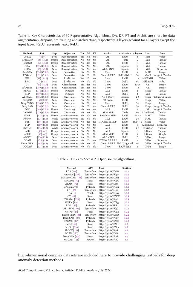
28 Pang, et al.
Table 1. Key Characteristics of 30 Representative Algorithms. DA, DP, PT and Archit. are short for dataaugmentation, dropout, pre-training and architecture, respectively. # layers account for all layers except theinput layer. lReLU represents leaky ReLU.
Method Ref. Sup. Objective DA DP PT Archit. Activation # layers Loss DataOADA [66] (4) Semi Reconstruction Yes No No AE ReLU 3 MSE Video
Replicator [58] (5.1.1) Unsup. Reconstruction No No No AE Tanh 2 MSE TabularRandNet [29] (5.1.1) Unsup. Reconstruction No Yes Yes AE ReLU 3 MSE TabularRDA [176] (5.1.1) Semi Reconstruction No No No AE Sigmoid 2 MSE TabularUODA [93] (5.1.1) Semi Reconstruction No No Yes AE & RNN Sigmoid 4 MSE Sequence
AnoGAN [139] (5.1.2) Semi Generative No No No Conv. ReLU 4 MAE ImageEBGAN [171] (5.1.2) Semi Generative No No No Conv. & MLP ReLU/lReLU 3-4 GAN Image & TabularFFP [88] (5.1.3) Semi Predictive Yes No Yes Conv. ReLU 10 MAE/MSE VideoLSA [1] (5.1.3) Semi Predictive No No No Conv. lReLU 4-7 MSE & KL videoGT [49] (5.1.4) Semi Classification Yes Yes No Conv. ReLU 10-16 CE Image
E3Outlier [159] (5.1.4) Semi Classification Yes Yes No Conv. ReLU 10 CE ImageREPEN [114] (5.2.1) Unsup. Distance No No No MLP ReLU 1 Hinge TabularRDP [157] (5.2.1) Unsup. Distance No No No MLP lReLU 1 MSE Tabular
AE-1SVM [106] (5.2.2) Unsup. One-class No No No AE & Conv. Sigmoid 2-5 Hinge Tabular & imageDeepOC [162](5.2.2) Semi One-class No No No 3D Conv. ReLU 5 Hinge Video
Deep SVDD [133] (5.2.2) Semi One-class No No Yes Conv. lReLU 3-4 Hinge ImageDeep SAD [134] (5.2.2) Semi One-class No No Yes Conv. & MLP lReLU 3-4 Hinge Image & Tabular
DEC [163] (5.2.3) Unsup. Clustering No Yes Yes MLP ReLU 4 KL Image & TabularDAGMM [179] (5.2.3) Unsup. Clustering No Yes No AE & MLP Tanh 4-6 Likelihood TabularSDOR [118] (6.1) Unsup. Anomaly scores No No Yes ResNet & MLP ReLU 50 + 2 MAE VideoPReNet [115] (6.1) Weak Anomaly scores Yes No No MLP ReLU 2-4 MAE TabularMIL [146] (6.1) Weak Anomaly scores No Yes Yes 3DConv. & MLP ReLU 18/34 + 3 Hinge VideoPUP [109] (6.2) Unsup. Anomaly scores No No No MLP ReLU 3 Likelihood Sequence
DevNet [116] (6.2) Weak Anomaly scores No No No MLP ReLU 2-4 Deviation TabularAPE [30] (6.3) Unsup. Anomaly scores No No No MLP Sigmoid 3 Softmax TabularAEHE [46] (6.3) Unsup. Anomaly scores No No No AE & MLP ReLU 4 Softmax GraphALOCC [136] (6.4) Semi Anomaly scores Yes No No AE & CNN lReLU 5 GANs ImageOCAN [175] (6.4) Semi Anomaly scores No No Yes LSTM-AE & MLP ReLU 4 GANs Sequence
Fence GAN [105] (6.4) Semi Anomaly scores No Yes No Conv. & MLP lReLU/Sigmoid 4-5 GANs Image & TabularOCGAN [121] (6.4) Semi Anomaly scores No No No Conv. ReLU/Tanh 3 GANs Image
Table 2. Links to Access 23 Open-source Algorithms.
Method API Link SectionRDA [176] Tensorflow https://git.io/JfYG5 5.1.1
AnoGAN [139] Tensorflow https://git.io/JfGgc 5.1.2Fast AnoGAN [138] Tensorflow https://git.io/JfZRn 5.1.2
EBGAN [171] Keras https://git.io/JfGgG 5.1.2ALAD [172] Keras https://git.io/JfZ8v 5.1.2
GANomaly [3] PyTorch https://git.io/JfGgn 5.1.2FFP [88] Tensorflow https://git.io/Jf4pc 5.1.3LSA [1] Torch https://git.io/Jf4pW 5.1.3GT [49] Keras https://git.io/JfZRW 5.1.4
E3Outlier [159] PyTorch https://git.io/Jf4pl 5.1.4REPEN [114] Keras https://git.io/JfZRg 5.2.1RDP [157] PyTorch https://git.io/RDP 5.2.1
AE-1SVM [106] Tensorflow https://git.io/JfGgl 5.2.2OC-NN [27] Keras https://git.io/JfGgZ 5.2.2
Deep SVDD [133] Tensorflow https://git.io/JfZRR 5.2.2Deep SAD [134] PyTorch https://git.io/JfOkr 5.2.2DAGMM [179] PyTorch https://git.io/JfZR0 5.2.3
MIL [146] Keras https://git.io/JfZRz 6.1DevNet [116] Keras https://git.io/JfZRw 6.2ALOCC [136] Tensorflow https://git.io/Jf4p4 6.4OCAN [175] Tensorflow https://git.io/JfYGb 6.4
FenceGAN [105] Keras https://git.io/Jf4pR 6.4OCGAN [121] MXNet https://git.io/Jf4p0 6.4
high-dimensional complex datasets are included here to provide challenging testbeds for deepanomaly detection methods.
ACM Comput. Surv., Vol. xx, No. x, Article . Publication date: July 202x.
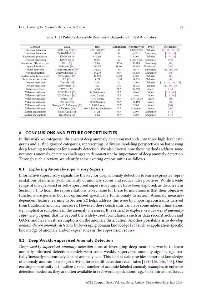
Deep Learning for Anomaly Detection: A Review 29
Table 3. 21 Publicly Accessible Real-world Datasets with Real Anomalies.
Domain Data Size Dimension Anomaly (%) Type ReferenceIntrusion detection KDD Cup 99 [13] 4,091-567,497 41 0.30%-7.70% Tabular [58, 105, 106, 179]Intrusion detection UNSW-NB15 [102] 257,673 49 ≤9.71% Streaming [115, 116]
Excitement prediction KDD Cup 14 619,326 10 6.00% Tabular [115, 116]Dropout prediction KDD Cup 15 35,091 27 0.10%-0.40% Sequence [93]
Malicious URLs detection URL [95] 2.4m 3.2m 33.04% Streaming [114]Spam detection Webspam [161] 350,000 16.6m 39.61% Tabular/text [114]Fraud detection Credit-card-fraud [34] 284,807 30 0.17% Streaming [115, 116, 175]Vandal detection UMDWikipedia [77] 34,210 N/A 50.00% Sequence [175]
Mutant activity detection p53 Mutants [35] 16,772 5,408 0.48% Tabular [114]Internet ads detection AD [13] 3,279 1,555 14.00% Tabular [114]Disease detection Thyroid [13] 7,200 21 7.40% Tabular [115, 116, 134, 179]Disease detection Arrhythmia [13] 452 279 14.60% Tabular [117, 134, 179]Defect detection MVTec AD 5,354 N/A 35.26% Image [15]Video surveillance UCSD Ped 1 [82] 14,000 frames N/A 28.6% Video [118, 162]Video surveillance UCSD Ped 2 [82] 4,560 frames N/A 35.9% Video [118, 162]Video surveillance UMN [108] 7,739 frames N/A 15.5%- 18.1% Video [118]Video surveillance Avenue [92] 30,652 frames N/A 12.46% Video [162]Video surveillance ShanghaiTech Campus [88] 317,398 frames N/A 5.38% Video [88]Video surveillance UCF-Crime [146] 1,900 videos (13.8m frames) N/A 13 crimes Video [146]System log analysis HDFS Log [165] 11.2m N/A 2.90% Sequence [41]System log analysis OpenStack log 1.3m N/A 7.00% Sequence [41]
8 CONCLUSIONS AND FUTURE OPPORTUNITIESIn this work we categorize the current deep anomaly detection methods into three high-level cate-gories and 11 fine-grained categories, representing 12 diverse modeling perspectives on harnessingdeep learning techniques for anomaly detection. We also discuss how these methods address somenotorious anomaly detection challenges to demonstrate the importance of deep anomaly detection.Through such a review, we identify some exciting opportunities as follows.
8.1 Exploring Anomaly-supervisory SignalsInformative supervisory signals are the key for deep anomaly detection to learn expressive repre-sentations of normality/abnormality or anomaly scores and reduce false positives. While a widerange of unsupervised or self-supervised supervisory signals have been explored, as discussed inSection 5.1, to learn the representations, a key issue for these formulations is that their objectivefunctions are generic but not optimized specifically for anomaly detection. Anomaly measure-dependent feature learning in Section 5.2 helps address this issue by imposing constraints derivedfrom traditional anomaly measures. However, these constraints can have some inherent limitations,e.g., implicit assumptions in the anomaly measures. It is critical to explore new sources of anomaly-supervisory signals that lie beyond the widely-used formulations such as data reconstruction andGANs, and have weak assumptions on the anomaly distribution. Another possibility is to developdomain-driven anomaly detection by leveraging domain knowledge [23] such as application-specificknowledge of anomaly and/or expert rules as the supervision source.
8.2 Deep Weakly-supervised Anomaly DetectionDeep weakly-supervised anomaly detection aims at leveraging deep neural networks to learnanomaly-informed detection models with some weakly-supervised anomaly signals, e.g., par-tially/inexactly/inaccurately labeled anomaly data. This labeled data provides important knowledgeof anomaly and can be a major driving force to lift detection recall rates [114–116, 146, 148]. Oneexciting opportunity is to utilize a small number of accurate labeled anomaly examples to enhancedetection models as they are often available in real-world applications, e.g., some intrusions/frauds
ACM Comput. Surv., Vol. xx, No. x, Article . Publication date: July 202x.

30 Pang, et al.
from deployed detection systems/end-users and verified by human experts. However, since anom-alies can be highly heterogeneous, there can be unknown/novel anomalies that lie beyond thespan set of the given anomaly examples. Thus, one important direction here is unknown anomalydetection, in which we aim to build detection models that are generalized from the limited labeledanomalies to unknown anomalies. Some recent studies [115, 116, 134] show that deep detectionmodels are able to learn abnormality that lie beyond the scope of the given anomaly examples. Itwould be important to further understand and explore the extent of the generalizability and todevelop models to further improve the accuracy performance.To detect anomalies that belong to the same classes of the given anomaly examples can be
as important as the detection of novel/unknown anomalies. Thus, another important directionis to develop data-efficient anomaly detection or few-shot anomaly detection, in which we aimat learning highly expressive representations of the known anomaly classes given only limitedanomaly examples [114–116, 153]. It should be noted that the limited anomaly examples may comefrom different anomaly classes and thus exhibit completely different manifold/class features. Thisscenarios is fundamentally different from the general few-shot learning [160], in which the limitedexamples are class-specific and assumed to share the same manifold/class structure. Additionally,as shown in Table 1, the network architectures are mostly not as deep as that in other machinelearning tasks. This may be partially due to the limitation of the labeled training data size. It isimportant to explore the possibility of leveraging those small labeled data to learn more powerfuldetection models with deeper architectures.
Also, inexact or inaccurate (e.g., coarse-grained) anomaly labels are often inexpensive to collectin some applications [146]; learning deep detection models with this weak supervision is importantin these scenarios.
8.3 Large-scale Normality LearningLarge-scale unsupervised/self-supervised representation learning has gained tremendous successin enabling downstream learning tasks [36, 123]. This is particular important for learning tasks, inwhich it is difficult to obtain sufficient labeled data, such as anomaly detection (see Section 2.1). Thegoal is to learn transferable pre-trained representation models from large-scale unlabeled data inan unsupervised/self-supervised mode and fine-tune detection models in a semi-supervised mode.The self-supervised classification-based methods in Section 5.1.3 may provide some initial sourcesof supervision for the normality learning. However, precautions must be taken to ensure that (i) theunlabeled data is free of anomaly contamination and/or (ii) the representation learning methods arerobust w.r.t. possible anomaly contamination. This is because most methods in Sections 5 implicitlyassume that the training data is clean and does not contain any noise/anomaly instances. Thisrobustness is important in both the pre-trained modeling and the fine-tuning stage. Additionally,anomalies and datasets in different domains vary significantly, so the large-scale normality learningmay need to be domain/application-specific.
8.4 Deep Detection of Complex AnomaliesMost of existing deep anomaly detection methods focus on point anomalies, showing substan-tially better performance than traditional methods. However, deep models for conditional/groupanomalies have been significantly less explored. Deep learning has superior capability in cap-turing complex temporal/spatial dependence and learning representations of a set of unordereddata points; it is important to explore whether deep learning could also gain similar advantagesover traditional approaches in detecting such complex anomalies. Novel neural network layers orobjectives functions may be required.
ACM Comput. Surv., Vol. xx, No. x, Article . Publication date: July 202x.
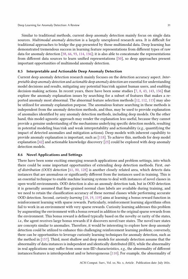
Deep Learning for Anomaly Detection: A Review 31
Similar to traditional methods, current deep anomaly detection mainly focus on single datasources. Multimodal anomaly detection is a largely unexplored research area. It is difficult fortraditional approaches to bridge the gap presented by those multimodal data. Deep learning hasdemonstrated tremendous success in learning feature representations from different types of rawdata for anomaly detection [38, 66, 93, 114, 136]; it is also able to concatenate the representationsfrom different data sources to learn unified representations [50], so deep approaches presentimportant opportunities of multimodal anomaly detection.
8.5 Interpretable and Actionable Deep Anomaly DetectionCurrent deep anomaly detection research mainly focuses on the detection accuracy aspect. Inter-pretable deep anomaly detection and actionable deep anomaly detection are essential for understandingmodel decisions and results, mitigating any potential bias/risk against human users, and enablingdecision-making actions. In recent years, there have been some studies [7, 8, 43, 143, 156] thatexplore the anomaly explanation issues by searching for a subset of features that makes a re-ported anomaly most abnormal. The abnormal feature selection methods [12, 112, 113] may alsobe utilized for anomaly explanation purpose. The anomalous feature searching in these methods isindependent from the anomaly detection methods, and thus, may be used to provide explanationof anomalies identified by any anomaly detection methods, including deep models. On the otherhand, this model-agnostic approach may render the explanation less useful, because they cannotprovide a genuine understanding of the mechanisms underlying specific detection models, resultingin potential modeling bias/risk and weak interpretability and actionability (e.g., quantifying theimpact of detected anomalies and mitigation actions). Deep models with inherent capability toprovide anomaly explanation is important, such as [118]. To achieve this, methods for deep modelexplanation [42] and actionable knowledge discovery [23] could be explored with deep anomalydetection models.
8.6 Novel Applications and SettingsThere have been some exciting emerging research applications and problem settings, into whichthere could be some important opportunities of extending deep detection methods. First, out-of-distribution (OOD) detection [61, 80, 128] is another closely related area, which detects datainstances that are anomalous or significantly different from the instances used in training. This isan essential technique to enable machine learning systems to deal with instances of novel classes inopen-world environments. OOD detection is also an anomaly detection task, but in OOD detectionit is generally assumed that fine-grained normal class labels are available during training, andwe need to retain the classification accuracy of these normal classes while performing accurateOOD detection. Second, curiosity learning [18, 19, 119] aims at learning a bonus reward function inreinforcement learning with sparse rewards. Particularly, reinforcement learning algorithms oftenfail to work in an environment with very sparse rewards. Curiosity learning addresses this problemby augmenting the environment with a bonus reward in addition to the original sparse rewards fromthe environment. This bonus reward is defined typically based on the novelty or rarity of the states,i.e., the agent receives large bonus rewards if it discovers novel/rare states. The novel/rare statesare concepts similar to anomalies. Therefore, it would be interesting to explore how deep anomalydetection could be utilized to enhance this challenging reinforcement learning problem; conversely,there can be opportunities to leverage curiosity learning techniques for anomaly detection, such asthe method in [157]. Third, most shallow and deep models for anomaly detection assume that theabnormality of data instances is independent and identically distributed (IID), while the abnormalityin real applications may suffer from some non-IID characteristics, e.g., the abnormality of differentinstances/features is interdependent and/or heterogeneous [110]. For example, the abnormality of
ACM Comput. Surv., Vol. xx, No. x, Article . Publication date: July 202x.
32 Pang, et al.
multiple synchronized disease symptoms is mutually reinforced in early detection of diseases. Thisrequires non-IID anomaly detection [110] that is dedicated to learning such non-IID abnormality.This task is crucial in complex scenarios, e.g., where anomalies have only subtle deviations andare hidden in the data space if not considering these non-IID abnormality characteristics. Lastly,other interesting applications include detection of adversarial examples [52, 120], anti-spoofing inbiometric systems [47, 122], and early detection of rare catastrophic events (e.g., financial crisis[24] and other black swan events [11]).
REFERENCES[1] Davide Abati, Angelo Porrello, Simone Calderara, and Rita Cucchiara. 2019. Latent space autoregression for novelty detection. In
CVPR. 481–490.[2] Charu C Aggarwal. 2017. Outlier analysis. Springer.[3] Samet Akcay, Amir Atapour-Abarghouei, and Toby P Breckon. 2018. GANomaly: Semi-supervised anomaly detection via adversarial
training. In ACCV. Springer, 622–637.[4] Leman Akoglu, Hanghang Tong, and Danai Koutra. 2015. Graph based anomaly detection and description: a survey. Data Mining and
Knowledge Discovery 29, 3 (2015), 626–688.[5] Elie Aljalbout, Vladimir Golkov, Yawar Siddiqui, Maximilian Strobel, and Daniel Cremers. 2018. Clustering with deep learning: Tax-
onomy and new methods. arXiv preprint arXiv:1801.07648 (2018).[6] J Andrews, Thomas Tanay, Edward J Morton, and Lewis D Griffin. 2016. Transfer representation-learning for anomaly detection. In
PMLR.[7] Fabrizio Angiulli, Fabio Fassetti, Giuseppe Manco, and Luigi Palopoli. 2017. Outlying property detection with numerical attributes.
Data mining and knowledge discovery 31, 1 (2017), 134–163.[8] Fabrizio Angiulli, Fabio Fassetti, and Luigi Palopoli. 2009. Detecting outlying properties of exceptional objects. ACM Transactions on
Database Systems 34, 1 (2009), 1–62.[9] Fabrizio Angiulli and Clara Pizzuti. 2002. Fast outlier detection in high dimensional spaces. In PKDD. Springer, 15–27.[10] Martin Arjovsky, Soumith Chintala, and Léon Bottou. 2017. Wasserstein Generative Adversarial Networks. In ICML. 214–223.[11] Terje Aven. 2016. Risk assessment and risk management: Review of recent advances on their foundation. European Journal of
Operational Research 253, 1 (2016), 1–13.[12] Fatemeh Azmandian, Ayse Yilmazer, Jennifer G Dy, Javed A Aslam, and David R Kaeli. 2012. GPU-accelerated feature selection for
outlier detection using the local kernel density ratio. In ICDM. IEEE, 51–60.[13] Kevin Bache and Moshe Lichman. 2013. UCI machine learning repository. URL http://archive. ics. uci. edu/ml 901 (2013).[14] Yoshua Bengio, Aaron Courville, and Pascal Vincent. 2013. Representation learning: A review and new perspectives. IEEE Transactions
on Pattern Analysis and Machine Intelligence 35, 8 (2013), 1798–1828.[15] Paul Bergmann, Michael Fauser, David Sattlegger, and Carsten Steger. 2019. MVTec AD–A Comprehensive Real-World Dataset for
Unsupervised Anomaly Detection. In CVPR. 9592–9600.[16] Azzedine Boukerche, Lining Zheng, and Omar Alfandi. 2020. Outlier Detection: Methods, Models and Classifications. Comput. Surveys
(2020).[17] Markus M Breunig, Hans-Peter Kriegel, Raymond T Ng, and Jörg Sander. 2000. LOF: Identifying density-based local outliers. ACM
SIGMOD Record 29, 2 (2000), 93–104.[18] Yuri Burda, Harri Edwards, Deepak Pathak, Amos Storkey, Trevor Darrell, and Alexei A Efros. 2019. Large-scale study of curiosity-
driven learning. In ICLR.[19] Yuri Burda, Harrison Edwards, Amos Storkey, and Oleg Klimov. 2019. Exploration by random network distillation. In ICLR.[20] Guilherme O Campos, Arthur Zimek, Jörg Sander, Ricardo JGB Campello, Barbora Micenková, Erich Schubert, Ira Assent, and
Michael E Houle. 2016. On the evaluation of unsupervised outlier detection: Measures, datasets, and an empirical study. Data Miningand Knowledge Discovery 30, 4 (2016), 891–927.
[21] Emmanuel J Candès, Xiaodong Li, Yi Ma, and John Wright. 2011. Robust principal component analysis? J. ACM 58, 3 (2011), 1–37.[22] Longbing Cao. 2015. Coupling learning of complex interactions. Information Processing & Management 51, 2 (2015), 167–186.[23] Longbing Cao, Philip S Yu, Chengqi Zhang, and Yanchang Zhao. 2010. Domain Driven Data Mining. Springer.[24] Wei Cao and Longbing Cao. 2015. Financial Crisis Forecasting via Coupled Market State Analysis. IEEE Intelligent Systems 30, 2 (2015),
18–25.[25] Mathilde Caron, Piotr Bojanowski, Armand Joulin, and Matthijs Douze. 2018. Deep clustering for unsupervised learning of visual
features. In ECCV. 132–149.[26] Raghavendra Chalapathy and Sanjay Chawla. 2019. Deep learning for anomaly detection: A survey. arXiv preprint arXiv:1901.03407
(2019).[27] Raghavendra Chalapathy, Aditya Krishna Menon, and Sanjay Chawla. 2018. Anomaly detection using one-class neural networks.
arXiv preprint arXiv:1802.06360 (2018).[28] Varun Chandola, Arindam Banerjee, and Vipin Kumar. 2009. Anomaly detection: A survey. Comput. Surveys 41, 3 (2009), 15.[29] Jinghui Chen, Saket Sathe, Charu Aggarwal, and Deepak Turaga. 2017. Outlier detection with autoencoder ensembles. In SDM. SIAM,
90–98.[30] Ting Chen, Lu-An Tang, Yizhou Sun, Zhengzhang Chen, and Kai Zhang. 2016. Entity embedding-based anomaly detection for het-
erogeneous categorical events. In IJCAI. 1396–1403.[31] Corinna Cortes and Vladimir Vapnik. 1995. Support-vector networks. Machine Learning 20, 3 (1995), 273–297.[32] Antonia Creswell, Tom White, Vincent Dumoulin, Kai Arulkumaran, Biswa Sengupta, and Anil A Bharath. 2018. Generative adver-
sarial networks: An overview. IEEE Signal Processing Magazine 35, 1 (2018), 53–65.[33] Zihang Dai, Zhilin Yang, Fan Yang, William W Cohen, and Russ R Salakhutdinov. 2017. Good semi-supervised learning that requires
a bad gan. In NeurIPS. 6510–6520.
ACM Comput. Surv., Vol. xx, No. x, Article . Publication date: July 202x.

Deep Learning for Anomaly Detection: A Review 33
[34] Andrea Dal Pozzolo, Giacomo Boracchi, Olivier Caelen, Cesare Alippi, and Gianluca Bontempi. 2017. Credit card fraud detection: arealistic modeling and a novel learning strategy. IEEE Transactions on Neural Networks and Learning Systems 29, 8 (2017), 3784–3797.
[35] Samuel A Danziger, Roberta Baronio, Lydia Ho, Linda Hall, Kirsty Salmon, G Wesley Hatfield, Peter Kaiser, and Richard H Lathrop.2009. Predicting positive p53 cancer rescue regions usingMost Informative Positive (MIP) active learning. PLoS Computational Biology5, 9 (2009).
[36] Jacob Devlin, Ming-Wei Chang, Kenton Lee, and Kristina Toutanova. 2018. Bert: Pre-training of deep bidirectional transformers forlanguage understanding. arXiv preprint arXiv:1810.04805 (2018).
[37] Nat Dilokthanakul, Pedro AMMediano, Marta Garnelo, Matthew CH Lee, Hugh Salimbeni, Kai Arulkumaran, and Murray Shanahan.2017. Deep unsupervised clustering with gaussian mixture variational autoencoders. In ICLR.
[38] Kaize Ding, Jundong Li, Rohit Bhanushali, and Huan Liu. 2019. Deep anomaly detection on attributed networks. In SDM. SIAM,594–602.
[39] Carl Doersch. 2016. Tutorial on variational autoencoders. arXiv preprint arXiv:1606.05908 (2016).[40] Jeff Donahue, Philipp Krähenbühl, and Trevor Darrell. 2017. Adversarial feature learning. In ICLR.[41] Min Du, Feifei Li, Guineng Zheng, and Vivek Srikumar. 2017. Deeplog: Anomaly detection and diagnosis from system logs through
deep learning. In CCS. 1285–1298.[42] Mengnan Du, Ninghao Liu, and Xia Hu. 2019. Techniques for interpretable machine learning. Commun. ACM 63, 1 (2019), 68–77.[43] Lei Duan, Guanting Tang, Jian Pei, James Bailey, Akiko Campbell, and Changjie Tang. 2015. Mining outlying aspects on numeric data.
Data Mining and Knowledge Discovery 29, 5 (2015), 1116–1151.[44] Andrew F Emmott, Shubhomoy Das, Thomas Dietterich, Alan Fern, andWeng-KeenWong. 2013. Systematic construction of anomaly
detection benchmarks from real data. In KDD Workshop. 16–21.[45] Sarah M Erfani, Sutharshan Rajasegarar, Shanika Karunasekera, and Christopher Leckie. 2016. High-dimensional and large-scale
anomaly detection using a linear one-class SVM with deep learning. Pattern Recognition 58 (2016), 121–134.[46] Shaohua Fan, Chuan Shi, and Xiao Wang. 2018. Abnormal event detection via heterogeneous information network embedding. In
CIKM. 1483–1486.[47] Soroush Fatemifar, Shervin Rahimzadeh Arashloo, Muhammad Awais, and Josef Kittler. 2019. Spoofing attack detection by anomaly
detection. In ICASSP. IEEE, 8464–8468.[48] Kamran Ghasedi Dizaji, Amirhossein Herandi, Cheng Deng, Weidong Cai, and Heng Huang. 2017. Deep clustering via joint convolu-
tional autoencoder embedding and relative entropy minimization. In ICCV. 5736–5745.[49] Izhak Golan and Ran El-Yaniv. 2018. Deep anomaly detection using geometric transformations. In NeurIPS. 9758–9769.[50] Ian Goodfellow, Yoshua Bengio, and Aaron Courville. 2016. Deep learning. MIT press.[51] Karol Gregor, Ivo Danihelka, Andriy Mnih, Charles Blundell, and Daan Wierstra. 2014. Deep AutoRegressive Networks. In ICML.
1242–1250.[52] Kathrin Grosse, Praveen Manoharan, Nicolas Papernot, Michael Backes, and Patrick McDaniel. 2017. On the (statistical) detection of
adversarial examples. arXiv preprint arXiv:1702.06280 (2017).[53] Frank E Grubbs. 1969. Procedures for detecting outlying observations in samples. Technometrics 11, 1 (1969), 1–21.[54] Manish Gupta, Jing Gao, Charu C Aggarwal, and Jiawei Han. 2013. Outlier detection for temporal data: A survey. IEEE Transactions
on Knowledge and Data Engineering 26, 9 (2013), 2250–2267.[55] Michael Gutmann and Aapo Hyvärinen. 2010. Noise-contrastive estimation: A new estimation principle for unnormalized statistical
models. In AISTATS. 297–304.[56] R. Hadsell, S. Chopra, and Y. LeCun. 2006. Dimensionality Reduction by Learning an Invariant Mapping. In CVPR, Vol. 2. 1735–1742.[57] Mahmudul Hasan, Jonghyun Choi, Jan Neumann, Amit K Roy-Chowdhury, and Larry S Davis. 2016. Learning temporal regularity in
video sequences. In CVPR. 733–742.[58] Simon Hawkins, Hongxing He, Graham Williams, and Rohan Baxter. 2002. Outlier detection using replicator neural networks. In
DaWaK.[59] Kaiming He, Xiangyu Zhang, Shaoqing Ren, and Jian Sun. 2016. Deep residual learning for image recognition. In CVPR. 770–778.[60] Zengyou He, Xiaofei Xu, and Shengchun Deng. 2003. Discovering cluster-based local outliers. Pattern Recognition Letters 24, 9-10
(2003), 1641–1650.[61] Dan Hendrycks and Kevin Gimpel. 2017. A baseline for detecting misclassified and out-of-distribution examples in neural networks.
In ICLR.[62] Geoffrey E Hinton and Ruslan R Salakhutdinov. 2006. Reducing the dimensionality of data with neural networks. Science 313, 5786
(2006), 504–507.[63] Victoria Hodge and Jim Austin. 2004. A survey of outlier detection methodologies. Artificial Intelligence Review 22, 2 (2004), 85–126.[64] Jun-Ting Hsieh, Bingbin Liu, De-An Huang, Li F Fei-Fei, and Juan Carlos Niebles. 2018. Learning to decompose and disentangle
representations for video prediction. In NeurIPS. 517–526.[65] Yi-an Huang, Wei Fan, Wenke Lee, and Philip S Yu. 2003. Cross-feature analysis for detecting ad-hoc routing anomalies. In ICDCS.
IEEE, 478–487.[66] Radu Tudor Ionescu, Fahad Shahbaz Khan, Mariana-Iuliana Georgescu, and Ling Shao. 2019. Object-centric auto-encoders and dummy
anomalies for abnormal event detection in video. In CVPR. 7842–7851.[67] Mon-Fong Jiang, Shian-Shyong Tseng, and Chih-Ming Su. 2001. Two-phase clustering process for outliers detection. Pattern recogni-
tion letters 22, 6-7 (2001), 691–700.[68] ShengYi Jiang, Xiaoyu Song, Hui Wang, Jian-Jun Han, and Qing-Hua Li. 2006. A clustering-based method for unsupervised intrusion
detections. Pattern Recognition Letters 27, 7 (2006), 802–810.[69] Xinwei Jiang, Junbin Gao, Xia Hong, and Zhihua Cai. 2014. Gaussian processes autoencoder for dimensionality reduction. In PAKDD.
Springer, 62–73.[70] Thorsten Joachims, Adith Swaminathan, and Tobias Schnabel. 2017. Unbiased learning-to-rank with biased feedback. In WSDM.
781–789.[71] Fabian Keller, Emmanuel Muller, and Klemens Bohm. 2012. HiCS: High contrast subspaces for density-based outlier ranking. In ICDE.
IEEE, 1037–1048.[72] Tung Kieu, Bin Yang, Chenjuan Guo, and Christian S Jensen. 2019. Outlier detection for time series with recurrent autoencoder
ensembles. In IJCAI.[73] Edwin M Knorr and Raymond T Ng. 1999. Finding intensional knowledge of distance-based outliers. In VLDB, Vol. 99. 211–222.
ACM Comput. Surv., Vol. xx, No. x, Article . Publication date: July 202x.
34 Pang, et al.
[74] Edwin M Knorr, Raymond T Ng, and Vladimir Tucakov. 2000. Distance-based outliers: algorithms and applications. The VLDB Journal8, 3-4 (2000), 237–253.
[75] Hans-Peter Kriegel, Peer Kroger, Erich Schubert, and Arthur Zimek. 2011. Interpreting and unifying outlier scores. In SDM. SIAM,13–24.
[76] Alex Krizhevsky, Ilya Sutskever, and Geoffrey E Hinton. 2012. Imagenet classification with deep convolutional neural networks. InNeurIPS. 1097–1105.
[77] Srijan Kumar, Francesca Spezzano, and VS Subrahmanian. 2015. Vews: A wikipedia vandal early warning system. In KDD. 607–616.[78] Aleksandar Lazarevic and Vipin Kumar. 2005. Feature bagging for outlier detection. In KDD. ACM, 157–166.[79] Yann LeCun, Léon Bottou, Yoshua Bengio, and Patrick Haffner. 1998. Gradient-based learning applied to document recognition. Proc.
IEEE 86, 11 (1998), 2278–2324.[80] Kimin Lee, Honglak Lee, Kibok Lee, and Jinwoo Shin. 2018. Training confidence-calibrated classifiers for detecting out-of-distribution
samples. In ICLR.[81] Ping Li, Trevor J Hastie, and Kenneth W Church. 2006. Very sparse random projections. In Proceedings of the 12th ACM SIGKDD
international conference on Knowledge discovery and data mining. 287–296.[82] Weixin Li, Vijay Mahadevan, and Nuno Vasconcelos. 2013. Anomaly detection and localization in crowded scenes. IEEE Transactions
on Pattern Analysis and Machine Intelligence 36, 1 (2013), 18–32.[83] Binbing Liao, Jingqing Zhang, ChaoWu, DouglasMcIlwraith, Tong Chen, Shengwen Yang, Yike Guo, and FeiWu. 2018. Deep sequence
learning with auxiliary information for traffic prediction. In KDD. 537–546.[84] Weixian Liao, Yifan Guo, Xuhui Chen, and Pan Li. 2018. A unified unsupervised gaussian mixture variational autoencoder for high
dimensional outlier detection. In IEEE Big Data. IEEE, 1208–1217.[85] Fei Tony Liu, Kai Ming Ting, and Zhi-Hua Zhou. 2012. Isolation-based anomaly detection. ACM Transactions on Knowledge Discovery
from Data 6, 1 (2012), 3.[86] Fei Tony Liu, Kai Ming Ting, and Zhi-Hua Zhou. 2012. Isolation-based anomaly detection. ACM Transactions on Knowledge Discovery
from Data 6, 1, Article 3 (2012), 3:1–3:39 pages.[87] Tie-Yan Liu et al. 2009. Learning to rank for information retrieval. Foundations and Trends® in Information Retrieval 3, 3 (2009),
225–331.[88] Wen Liu, Weixin Luo, Dongze Lian, and Shenghua Gao. 2018. Future frame prediction for anomaly detection–a new baseline. In CVPR.
6536–6545.[89] Xialei Liu, Joost van de Weijer, and Andrew D Bagdanov. 2018. Leveraging unlabeled data for crowd counting by learning to rank. In
CVPR. 7661–7669.[90] Yusha Liu, Chun-Liang Li, and Barnabás Póczos. 2018. Classifier Two Sample Test for Video Anomaly Detections.. In BMVC. 71.[91] Yezheng Liu, Zhe Li, Chong Zhou, Yuanchun Jiang, Jianshan Sun, Meng Wang, and Xiangnan He. 2019. Generative adversarial active
learning for unsupervised outlier detection. IEEE Transactions on Knowledge and Data Engineering (2019).[92] Cewu Lu, Jianping Shi, and Jiaya Jia. 2013. Abnormal event detection at 150 fps in matlab. In ICCV. 2720–2727.[93] Weining Lu, Yu Cheng, Cao Xiao, Shiyu Chang, Shuai Huang, Bin Liang, and Thomas Huang. 2017. Unsupervised sequential outlier
detection with deep architectures. IEEE Transactions on Image Processing 26, 9 (2017), 4321–4330.[94] Weixin Luo, Wen Liu, and Shenghua Gao. 2017. Remembering history with convolutional lstm for anomaly detection. In 2017 IEEE
International Conference on Multimedia and Expo (ICME). IEEE, 439–444.[95] Justin Ma, Lawrence K Saul, Stefan Savage, and Geoffrey M Voelker. 2009. Identifying suspicious URLs: An application of large-scale
online learning. In ICML. ACM, 681–688.[96] Vijay Mahadevan, Weixin Li, Viral Bhalodia, and Nuno Vasconcelos. 2010. Anomaly detection in crowded scenes. In CVPR. IEEE,
1975–1981.[97] Alireza Makhzani and Brendan Frey. 2014. K-sparse autoencoders. In ICLR.[98] Pankaj Malhotra, Anusha Ramakrishnan, Gaurangi Anand, Lovekesh Vig, Puneet Agarwal, and Gautam Shroff. 2016. LSTM-based
encoder-decoder for multi-sensor anomaly detection. arXiv preprint arXiv:1607.00148 (2016).[99] Erik Marchi, Fabio Vesperini, Felix Weninger, Florian Eyben, Stefano Squartini, and Björn Schuller. 2015. Non-linear prediction with
LSTM recurrent neural networks for acoustic novelty detection. In 2015 International Joint Conference on Neural Networks (IJCNN).IEEE, 1–7.
[100] Michael Mathieu, Camille Couprie, and Yann LeCun. 2016. Deep multi-scale video prediction beyond mean square error. In ICLR.[101] Luke Metz, Ben Poole, David Pfau, and Jascha Sohl-Dickstein. 2017. Unrolled generative adversarial networks. In ICLR.[102] Nour Moustafa and Jill Slay. 2015. UNSW-NB15: a comprehensive data set for network intrusion detection systems. In Military
Communications and Information Systems Conference, 2015. 1–6.[103] Mary M Moya, Mark W Koch, and Larry D Hostetler. 1993. One-class classifier networks for target recognition applications. Technical
Report. NASA STI/Recon Technical Report N.[104] Andrew Y Ng and Stuart J Russell. 2000. Algorithms for Inverse Reinforcement Learning. In ICML. Morgan Kaufmann Publishers Inc.,
663–670.[105] Cuong Phuc Ngo, Amadeus Aristo Winarto, Connie Kou Khor Li, Sojeong Park, Farhan Akram, and Hwee Kuan Lee. 2019. Fence
GAN: towards better anomaly detection. arXiv preprint arXiv:1904.01209 (2019).[106] Minh-Nghia Nguyen and Ngo Anh Vien. 2018. Scalable and interpretable one-class svms with deep learning and random fourier
features. In ECML-PKDD. Springer, 157–172.[107] Keith Noto, Carla Brodley, and Donna Slonim. 2012. FRaC: a feature-modeling approach for semi-supervised and unsupervised
anomaly detection. Data mining and knowledge discovery 25, 1 (2012), 109–133.[108] University of Minnesota. 2020. UMN Unusual Crowd Activity data set. http://mha.cs.umn.edu/Movies/Crowd-Activity-All.avi. Ac-
cessed: 2020-05-30.[109] Min-hwan Oh and Garud Iyengar. 2019. Sequential Anomaly Detection using Inverse Reinforcement Learning. In KDD. 1480–1490.[110] Guansong Pang. 2019. Non-IID outlier detection with coupled outlier factors. Ph.D. Dissertation.[111] Guansong Pang, Longbing Cao, Ling Chen, Defu Lian, and Huan Liu. 2018. Sparse modeling-based sequential ensemble learning for
effective outlier detection in high-dimensional numeric data. In AAAI. 3892–3899.[112] Guansong Pang, Longbing Cao, Ling Chen, and Huan Liu. 2016. Unsupervised feature selection for outlier detection by modelling
hierarchical value-feature couplings. In ICDM. IEEE, 410–419.
ACM Comput. Surv., Vol. xx, No. x, Article . Publication date: July 202x.
Deep Learning for Anomaly Detection: A Review 35
[113] Guansong Pang, Longbing Cao, Ling Chen, and Huan Liu. 2017. Learning homophily couplings from non-IID data for joint featureselection and noise-resilient outlier detection. In IJCAI. 2585–2591.
[114] Guansong Pang, Longbing Cao, Ling Chen, and Huan Liu. 2018. Learning Representations of Ultrahigh-dimensional Data for RandomDistance-based Outlier Detection. In KDD. 2041–2050.
[115] Guansong Pang, Chunhua Shen, Huidong Jin, and Anton van den Hengel. 2019. Deep Weakly-supervised Anomaly Detection. arXivpreprint arXiv:1910.13601 (2019).
[116] Guansong Pang, Chunhua Shen, and Anton van den Hengel. 2019. Deep Anomaly Detection with Deviation Networks. In KDD.353–362.
[117] Guansong Pang, Kai Ming Ting, and David Albrecht. 2015. LeSiNN: Detecting anomalies by identifying least similar nearest neigh-bours. In ICDM Workshop. IEEE, 623–630.
[118] Guansong Pang, Cheng Yan, Chunhua Shen, Anton van den Hengel, and Xiao Bai. 2020. Self-trained Deep Ordinal Regression forEnd-to-End Video Anomaly Detection. In CVPR. 12173–12182.
[119] Deepak Pathak, Pulkit Agrawal, Alexei A Efros, and Trevor Darrell. 2017. Curiosity-driven Exploration by Self-supervised Prediction.In ICML. 2778–2787.
[120] Andrea Paudice, Luis Muñoz-González, Andras Gyorgy, and Emil C Lupu. 2018. Detection of adversarial training examples in poison-ing attacks through anomaly detection. arXiv preprint arXiv:1802.03041 (2018).
[121] Pramuditha Perera, Ramesh Nallapati, and Bing Xiang. 2019. OCGAN: One-class novelty detection using gans with constrained latentrepresentations. In CVPR. 2898–2906.
[122] Daniel Pérez-Cabo, David Jiménez-Cabello, Artur Costa-Pazo, and Roberto J López-Sastre. 2019. Deep anomaly detection for gener-alized face anti-spoofing. In CVPR Workshops.
[123] Matthew E Peters, Mark Neumann, Mohit Iyyer, Matt Gardner, Christopher Clark, Kenton Lee, and Luke Zettlemoyer. 2018. Deepcontextualized word representations. In NAACL-HLT. 2227–2237.
[124] Tomáš Pevny. 2016. Loda: Lightweight on-line detector of anomalies. Machine Learning 102, 2 (2016), 275–304.[125] Ali Rahimi and Benjamin Recht. 2008. Random features for large-scale kernel machines. In NeurIPS. 1177–1184.[126] Sridhar Ramaswamy, Rajeev Rastogi, and Kyuseok Shim. 2000. Efficient algorithms formining outliers from large data sets. In SIGMOD.
427–438.[127] Sridhar Ramaswamy, Rajeev Rastogi, and Kyuseok Shim. 2000. Efficient algorithms for mining outliers from large data sets. ACM
SIGMOD Record 29, 2 (2000), 427–438.[128] Jie Ren, Peter J Liu, Emily Fertig, Jasper Snoek, Ryan Poplin, Mark Depristo, Joshua Dillon, and Balaji Lakshminarayanan. 2019.
Likelihood ratios for out-of-distribution detection. In NeurIPS. 14680–14691.[129] Salah Rifai, Pascal Vincent, Xavier Muller, Xavier Glorot, and Yoshua Bengio. 2011. Contractive auto-encoders: explicit invariance
during feature extraction. In ICML. 833–840.[130] Olaf Ronneberger, Philipp Fischer, and Thomas Brox. 2015. U-net: Convolutional networks for biomedical image segmentation. In
MICCAI. Springer, 234–241.[131] Lorenzo Rosasco, Ernesto De Vito, Andrea Caponnetto, Michele Piana, and Alessandro Verri. 2004. Are loss functions all the same?
Neural Computation 16, 5 (2004), 1063–1076.[132] Volker Roth. 2005. Outlier detection with one-class kernel fisher discriminants. In NeurIPS. 1169–1176.[133] Lukas Ruff, Nico Görnitz, Lucas Deecke, Shoaib Ahmed Siddiqui, Robert Vandermeulen, Alexander Binder, Emmanuel Müller, and
Marius Kloft. 2018. Deep one-class classification. In ICML. 4390–4399.[134] Lukas Ruff, Robert A Vandermeulen, Nico Görnitz, Alexander Binder, Emmanuel Müller, Klaus-Robert Müller, and Marius Kloft. 2020.
Deep semi-supervised anomaly detection. ICLR.[135] Olga Russakovsky, Jia Deng, Hao Su, Jonathan Krause, Sanjeev Satheesh, Sean Ma, Zhiheng Huang, Andrej Karpathy, Aditya Khosla,
Michael Bernstein, et al. 2015. Imagenet large scale visual recognition challenge. International journal of computer vision 115, 3 (2015),211–252.
[136] Mohammad Sabokrou, Mohammad Khalooei, Mahmood Fathy, and Ehsan Adeli. 2018. Adversarially learned one-class classifier fornovelty detection. In CVPR. 3379–3388.
[137] Tim Salimans, Ian Goodfellow, Wojciech Zaremba, Vicki Cheung, Alec Radford, and Xi Chen. 2016. Improved techniques for traininggans. In NeurIPS. 2234–2242.
[138] Thomas Schlegl, Philipp Seeböck, Sebastian M Waldstein, Georg Langs, and Ursula Schmidt-Erfurth. 2019. f-AnoGAN: Fast unsuper-vised anomaly detection with generative adversarial networks. Medical Image Analysis 54 (2019), 30–44.
[139] Thomas Schlegl, Philipp Seeböck, Sebastian M Waldstein, Ursula Schmidt-Erfurth, and Georg Langs. 2017. Unsupervised anomalydetection with generative adversarial networks to guide marker discovery. In IPMI. Springer, Cham, 146–157.
[140] Bernhard Schölkopf, John C Platt, John Shawe-Taylor, Alex J Smola, and Robert C Williamson. 2001. Estimating the support of ahigh-dimensional distribution. Neural Computation 13, 7 (2001), 1443–1471.
[141] Bernhard Schölkopf, Alexander Smola, and Klaus-Robert Müller. 1997. Kernel principal component analysis. In ICANN. Springer,583–588.
[142] Erich Schubert, Jörg Sander, Martin Ester, Hans Peter Kriegel, and Xiaowei Xu. 2017. DBSCAN revisited, revisited: why and how youshould (still) use DBSCAN. ACM Transactions on Database Systems 42, 3 (2017), 1–21.
[143] Md Amran Siddiqui, Alan Fern, Thomas G Dietterich, and Weng-Keen Wong. 2019. Sequential feature explanations for anomalydetection. ACM Transactions on Knowledge Discovery from Data 13, 1 (2019), 1–22.
[144] Karen Simonyan and Andrew Zisserman. 2015. Very deep convolutional networks for large-scale image recognition. In ICLR.[145] Mahito Sugiyama and Karsten Borgwardt. 2013. Rapid distance-based outlier detection via sampling. In NeurIPS. 467–475.[146] Waqas Sultani, Chen Chen, and Mubarak Shah. 2018. Real-world anomaly detection in surveillance videos. In CVPR. 6479–6488.[147] Ilya Sutskever, Oriol Vinyals, and Quoc V Le. 2014. Sequence to sequence learning with neural networks. In NeurIPS. 3104–3112.[148] Acar Tamersoy, Kevin Roundy, and Duen Horng Chau. 2014. Guilt by association: Large scale malware detection by mining file-
relation graphs. In KDD. 1524–1533.[149] David MJ Tax and Robert PW Duin. 2004. Support vector data description. Machine Learning 54, 1 (2004), 45–66.[150] Lena Tenenboim-Chekina, Lior Rokach, and Bracha Shapira. 2013. Ensemble of feature chains for anomaly detection. InMCS. Springer,
295–306.[151] Lucas Theis, Wenzhe Shi, Andrew Cunningham, and Ferenc Huszár. 2017. Lossy image compression with compressive autoencoders.
In ICLR.
ACM Comput. Surv., Vol. xx, No. x, Article . Publication date: July 202x.

36 Pang, et al.
[152] Fei Tian, Bin Gao, Qing Cui, Enhong Chen, and Tie-Yan Liu. 2014. Learning deep representations for graph clustering. In AAAI.1293–1299.
[153] Yu Tian, Gabriel Maicas, Leonardo Zorron Cheng Tao Pu, Rajvinder Singh, Johan W. Verjans, and Gustavo Carneiro. 2020. Few-ShotAnomaly Detection for Polyp Frames from Colonoscopy. In MICCAI.
[154] Radu Tudor Ionescu, Sorina Smeureanu, Bogdan Alexe, and Marius Popescu. 2017. Unmasking the abnormal events in video. In ICCV.2895–2903.
[155] Pascal Vincent, Hugo Larochelle, Isabelle Lajoie, Yoshua Bengio, and Pierre-Antoine Manzagol. 2010. Stacked denoising autoencoders:Learning useful representations in a deep networkwith a local denoising criterion. Journal ofMachine Learning Research 11, Dec (2010),3371–3408.
[156] Nguyen Xuan Vinh, Jeffrey Chan, Simone Romano, James Bailey, Christopher Leckie, Kotagiri Ramamohanarao, and Jian Pei. 2016.Discovering outlying aspects in large datasets. Data Mining and Knowledge Discovery 30, 6 (2016), 1520–1555.
[157] Hu Wang, Guansong Pang, Chunhua Shen, and Congbo Ma. 2020. Unsupervised Representation Learning by Predicting RandomDistances. In IJCAI.
[158] Hao Wang and Dit-Yan Yeung. 2016. Towards Bayesian deep learning: A framework and some existing methods. IEEE Transactionson Knowledge and Data Engineering 28, 12 (2016), 3395–3408.
[159] Siqi Wang, Yijie Zeng, Xinwang Liu, En Zhu, Jianping Yin, Chuanfu Xu, and Marius Kloft. 2019. Effective End-to-end UnsupervisedOutlier Detection via Inlier Priority of Discriminative Network. In NeurIPS. 5960–5973.
[160] Yaqing Wang, Quanming Yao, James T Kwok, and Lionel M Ni. [n.d.]. Generalizing from a few examples: A survey on few-shotlearning. Comput. Surveys ([n. d.]).
[161] Steve Webb, James Caverlee, and Calton Pu. 2006. Introducing the Webb Spam Corpus: Using Email Spam to Identify Web SpamAutomatically.. In CEAS.
[162] PengWu, Jing Liu, and Fang Shen. 2019. A Deep One-Class Neural Network for Anomalous Event Detection in Complex Scenes. IEEETransactions on Neural Networks and Learning Systems (2019).
[163] Junyuan Xie, Ross Girshick, and Ali Farhadi. 2016. Unsupervised deep embedding for clustering analysis. In ICML. 478–487.[164] Dan Xu, Elisa Ricci, Yan Yan, Jingkuan Song, and Nicu Sebe. 2015. Learning Deep Representations of Appearance and Motion for
Anomalous Event Detection. In British Machine Vision Conference.[165] Wei Xu, Ling Huang, Armando Fox, David Patterson, and Michael Jordan. 2009. Online system problem detection by mining patterns
of console logs. In ICDM. IEEE, 588–597.[166] Jianwei Yang, Devi Parikh, and Dhruv Batra. 2016. Joint unsupervised learning of deep representations and image clusters. In CVPR.
5147–5156.[167] Xu Yang, Cheng Deng, Feng Zheng, Junchi Yan, andWei Liu. 2019. Deep spectral clustering using dual autoencoder network. In CVPR.
4066–4075.[168] Muchao Ye, Xiaojiang Peng, Weihao Gan, Wei Wu, and Yu Qiao. 2019. Anopcn: Video anomaly detection via deep predictive coding
network. In ACM MM. 1805–1813.[169] Wenchao Yu, Wei Cheng, Charu C Aggarwal, Kai Zhang, Haifeng Chen, and Wei Wang. 2018. Netwalk: A flexible deep embedding
approach for anomaly detection in dynamic networks. In KDD. 2672–2681.[170] Muhammad Zaigham Zaheer, Jin-ha Lee, Marcella Astrid, and Seung-Ik Lee. 2020. Old is Gold: Redefining the Adversarially Learned
One-Class Classifier Training Paradigm. In CVPR. 14183–14193.[171] Houssam Zenati, Chuan Sheng Foo, Bruno Lecouat, Gaurav Manek, and Vijay Ramaseshan Chandrasekhar. 2018. Efficient gan-based
anomaly detection. arXiv preprint arXiv:1802.06222 (2018).[172] Houssam Zenati, Manon Romain, Chuan-Sheng Foo, Bruno Lecouat, and Vijay Chandrasekhar. 2018. Adversarially learned anomaly
detection. In ICDM. IEEE, 727–736.[173] Chuxu Zhang, Dongjin Song, Yuncong Chen, Xinyang Feng, Cristian Lumezanu, Wei Cheng, Jingchao Ni, Bo Zong, Haifeng Chen,
and Nitesh V Chawla. 2019. A deep neural network for unsupervised anomaly detection and diagnosis in multivariate time seriesdata. In AAAI, Vol. 33. 1409–1416.
[174] Ke Zhang, Marcus Hutter, and Huidong Jin. 2009. A new local distance-based outlier detection approach for scattered real-world data.In PAKDD. Springer, 813–822.
[175] Panpan Zheng, Shuhan Yuan, Xintao Wu, Jun Li, and Aidong Lu. 2019. One-class adversarial nets for fraud detection. In AAAI.1286–1293.
[176] Chong Zhou and Randy C Paffenroth. 2017. Anomaly detection with robust deep autoencoders. In KDD. ACM, 665–674.[177] Jun-Yan Zhu, Taesung Park, Phillip Isola, and Alexei A Efros. 2017. Unpaired image-to-image translation using cycle-consistent
adversarial networks. In ICCV. 2223–2232.[178] Arthur Zimek, Erich Schubert, and Hans-Peter Kriegel. 2012. A survey on unsupervised outlier detection in high-dimensional numer-
ical data. Statistical Analysis and Data Mining 5, 5 (2012), 363–387.[179] Bo Zong, Qi Song, Martin Renqiang Min, Wei Cheng, Cristian Lumezanu, Daeki Cho, and Haifeng Chen. 2018. Deep autoencoding
gaussian mixture model for unsupervised anomaly detection. In ICLR.[180] Hui Zou, Trevor Hastie, and Robert Tibshirani. 2006. Sparse principal component analysis. Journal of computational and graphical
statistics 15, 2 (2006), 265–286.
ACM Comput. Surv., Vol. xx, No. x, Article . Publication date: July 202x.

![arXiv:1601.05610v1 [cs.CV] 21 Jan 2016 · arXiv:1601.05610v1 [cs.CV] 21 Jan 2016. 2 Hui Li, Chunhua Shen CNN based text string detection False positives elimination by heuristic rules](https://img.pdfslide.net/doc/110x75/5f724fd85f31467d9023dc51/arxiv160105610v1-cscv-21-jan-2016-arxiv160105610v1-cscv-21-jan-2016-2.jpg)