Circularly Polarized Microstrip Antenna

Marwa Shakeeb

A Thesis

In

The Department

of

Electrical and Computer Engineering

Concordia University

Presented in Partial Fulfillment of the Requirements

for the Degree of Master of Applied Science (Electrical Engineering) at

Concordia University

Montreal, Quebec, Canada

December 2010

© Marwa Shakeeb

CONCORDIA UNIVERSITY

SCHOOL OF GRADUATE STUDIES

This is to certify that the thesis prepared

By: Marwa Shakeeb

Entitled: “Circularly Polarized Microstrip Antenna”

and submitted in partial fulfillment of the requirements for the degree of

Master of Applied Science

Complies with the regulations of this University and meets the accepted standards with

respect to originality and quality.

Signed by the final examining committee:

________________________________________________ Chair

Dr. D. Qiu

________________________________________________ Examiner, External

Dr. A. Ben Hamza, CIISE To the Program

________________________________________________ Examiner

Dr. T. Denidni

________________________________________________ Supervisor

Dr. A. Sebak

Approved by: ___________________________________________

Dr. W. E. Lynch, Chair

Department of Electrical and Computer Engineering

____________20_____ ___________________________________

Dr. Robin A. L. Drew

Dean, Faculty of Engineering and

Computer Science

iii

Abstract

Circularly Polarized Microstrip Antenna

Marwa Shakeeb

Matching the polarization in both the transmitter and receiver antennas is important in

terms of decreasing transmission losses. The use of circularly polarized antennas presents

an attractive solution to achieve this polarization match which allows for more flexibility

in the angle between transmitting and receiving antennas, reduces the effect of multipath

reflections, enhances weather penetration and allows for the mobility of both the

transmitter and the receiver.

The objective of this thesis is to design a single fed circularly polarized microstrip

antenna that operates at 2.4 GHz. Single feeding is used because it is simple, easy to

manufacture, low in cost and compact in structure. This thesis presents a new design for a

circularly polarized antenna based on a circular microstrip patch. Circular polarization is

generated by truncating two opposite edges from a circular patch antenna at 45° to the

feed. The truncation splits the field into two orthogonal modes with equal magnitude and

90° phase shift. The perturbation dimensions are then optimized to achieve the low axial

ratio required to achieve circular polarization at the desired frequency. This thesis

presents three design variations. The first design is fed by microstrip line feed, the second

is fed by proximity feeding and the third is fed by aperture feeding. The design of the

microstrip fed antenna requires parametric studies on the antenna diameter and the

distance between the patch center and the truncation. It also required designing a quarter

iv

wavelength transformer between the 50 feed line and the patch. The design of the

proximity fed antenna requires one additional parametric study on the length of the feed

line while the aperture fed antenna requires two additional parametric studies on the

length of the feed line and the diameter of the ground slot.

Results show that microstrip fed antenna design in this thesis can yield 8.11 dB directive

gain, axial ratio and impedance bandwidth 0.83 % and 2.92 % respectively. The

proximity fed antenna in this thesis can yield 8 dB directive gain, axial ratio and

impedance bandwidth 1.45 % and 5.36 % respectively. The aperture fed antenna in this

thesis can yield 7.92 dB directive gain, axial ratio and impedance bandwidth 0.83 % and

2.92 % respectively.

v

To Mohamed, Hana and Karim

vi

Acknowledgement

I would like to express my deepest appreciation and gratitude to my academic and

research advisor, Professor A. Sebak for his advice and invaluable guidance throughout

my research. This work would have been impossible without his precious support and

encouragement.

I would like to thank the members of my examining committee Dr. Abedesamad Ben

Hamza, Dr. Dongyu Qiu and Dr. Tayeb A. Denidni. I especially want to thank my

colleague Dr. Michael Wong for his help and support whenever needed. I would like to

thank Dr. Hany Hammad Associate Professor at GUC for his help and cooperation.

My deepest gratefulness goes to my husband Mohamed Ashour for his love, help and

support during my studies. I’m really lucky couldn’t have made it without him. Special

thanks to the wonderful mother I’m blessed with; Khadiga for her endless extraordinary

support in every aspect in my life. Last but not least I would like to thank my daughter

Hana and my son Karim for giving me the time to finish my studies.

vii

Table of Contents

Chapter 1 Introduction ................................................................................................... 1

1.1 Motivation ............................................................................................................ 2

1.2 Objective .............................................................................................................. 3

1.3 Thesis organization .............................................................................................. 3

Chapter 2 Circularly polarized microstrip patch antenna .............................................. 5

2.1 Advantages and disadvantages of microstrip antennas ........................................ 6

2.2 Microstrip antenna................................................................................................ 7

2.2.1 Metallic patch................................................................................................ 8

2.2.2 Dielectric substrate........................................................................................ 9

2.2.3 The ground .................................................................................................... 9

2.2.4 Feeding .......................................................................................................... 9

2.2.5 Methods of analysis .................................................................................... 14

2.3 Polarization......................................................................................................... 15

2.3.1 Types of polarization .................................................................................. 16

viii

2.4 Circular polarization and microstrip antenna ..................................................... 19

2.4.1 Dual feed circularly polarized microstrip antenna ...................................... 20

2.4.2 Single feed circularly polarized microstrip antenna ................................... 21

2.5 Single fed circularly polarized microstrip antenna ............................................ 22

2.6 Summary ............................................................................................................ 29

Chapter 3 Truncated edges circularly polarized microstrip antenna ........................... 31

3.1 Design methodology .......................................................................................... 32

3.2 Truncated edges circularly polarized antenna .................................................... 32

3.3 Microstrip feeding .............................................................................................. 33

3.4 Proximity feeding ............................................................................................... 39

3.5 Aperture feeding ................................................................................................. 47

3.6 Summary ............................................................................................................ 56

Chapter 4 Antenna design results and verifications .................................................... 57

4.1 Design verification for the 3 proposed antennas ................................................ 57

4.2 Fabrication and measured results ....................................................................... 60

4.3 HFSS simulation results for the 3 proposed antennas ........................................ 61

4.3.1 Microstrip feeding ....................................................................................... 61

4.3.2 Proximity feed line ...................................................................................... 64

4.3.3 Aperture feed line ....................................................................................... 67

4.4 Comparison between the 3 antennas .................................................................. 70

4.5 Summary ............................................................................................................ 70

Chapter 5 Conclusion and future work ........................................................................ 72

5.1 Conclusion .......................................................................................................... 72

ix

5.2 Future work ........................................................................................................ 74

References ......................................................................................................................... 75

Publications ....................................................................................................................... 79

x

List of Figures

Figure 2-1: Basic Microstrip antenna ................................................................................. 8

Figure 2-2 Different shapes for microstrip antenna ........................................................... 8

Figure 2-3 Coaxial feeding ............................................................................................... 10

Figure 2-4 Direct microstrip feed line .............................................................................. 11

Figure 2-5 Inset microstrip feed line ................................................................................ 12

Figure 2-6 Gap-coupled microstrip feed line .................................................................... 12

Figure 2-7 Proximity coupled microstrip feeding ............................................................. 13

Figure 2-8 Aperture coupled microstrip feed .................................................................... 14

Figure 2-9 Plane wave and its polarization ellipse @Z = 0 [12] ...................................... 17

Figure 2-10 Types of polarization..................................................................................... 17

Figure 2-11 Examples for dual fed CP patches [24] ......................................................... 20

Figure 2-12 single fed patches .......................................................................................... 21

xi

Figure 2-13 Microstrip square patch antenna with C-shaped slot [36] ............................. 23

Figure 2-14 Microstrip square patch antenna with F-shaped slot [7] ............................... 23

Figure 2-15 Microstrip square patch antenna with S-shaped slot [38] ............................. 24

Figure 2-16 Microstrip square patch antenna with 2 connected rectangular slots [40] .... 25

Figure 2-17 Circular patch with cross slot ........................................................................ 25

Figure 2-18 Circular patch with cross slot in the patch and ground plane [27] ................. 26

Figure 2-19 Stacked truncated corners square patches ..................................................... 27

Figure 2-20 Stacked square patch over square ring [30] .................................................. 27

Figure 2-21 Truncated corner square microstrip antenna with 4 slits [4] ......................... 28

Figure 2-22 Truncated edges elliptical antenna [5] .......................................................... 28

Figure 2-23 Truncated edges circular microstrip antenna [6] ........................................... 29

Figure 2-24 Annular ring with inner strip line [23] .......................................................... 29

Figure 3-1 Antenna with microstrip feed .......................................................................... 34

Figure 3-2 Perfect circle radius parametric study - microstrip feeding ............................ 36

Figure 3-3 Parametric analysis of (d) at 2.4 GHz - microstrip feeding ............................ 37

Figure 3-4 Return loss for (d) parametric study - microstrip feeding ............................... 38

Figure 3-5 Axial ratio for (d) parametric study - microstrip feeding ................................ 38

Figure 3-6 3D view for proximity fed antenna ................................................................. 39

Figure 3-7 Antenna fed by proximity feeding .................................................................. 40

xii

Figure 3-8 Perfect circle radius parametric study - proximity feeding ............................. 40

Figure 3-9 Parametric analysis of (d) at 2.4 GHz - proximity feeding ............................. 41

Figure 3-10 Return loss for (d) parametric study - proximity feeding ............................. 42

Figure 3-11 Axial ratio for (d) parametric study - proximity feeding .............................. 42

Figure 3-12 Parametric analysis of (Lf) at 2.4 GHz - proximity feeding .......................... 43

Figure 3-13 Return loss for (Lf) parametric study - proximity feeding ............................ 44

Figure 3-14 Axial ratio for (Lf) parametric study - proximity feeding ............................. 44

Figure 3-15 Return loss for re-determining (rad) - proximity feeding ............................. 45

Figure 3-16 Axial ratio for re-determining (rad) - proximity feeding .............................. 45

Figure 3-17 Return loss for re-determining (d) - proximity feeding ................................ 46

Figure 3-18 Axial ratio for re-determining (d) - proximity feeding ................................. 47

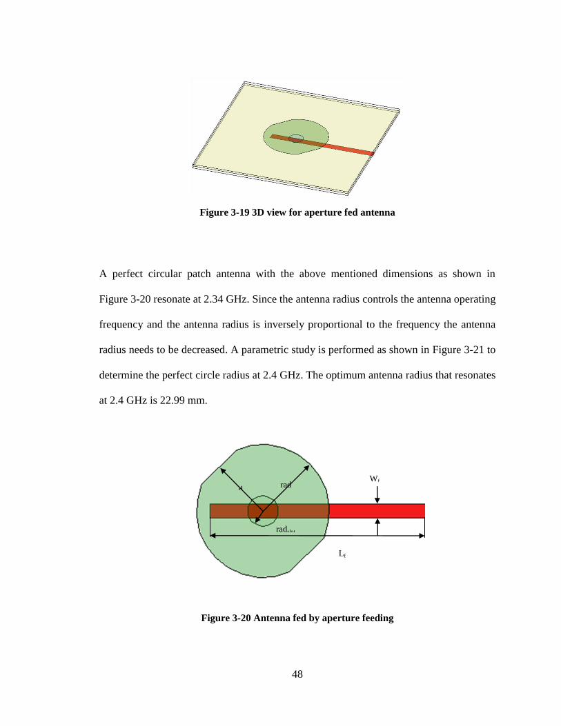
Figure 3-19 3D view for aperture fed antenna .................................................................. 48

Figure 3-20 Antenna fed by aperture feeding ................................................................... 48

Figure 3-21 Perfect circle radius parametric study - aperture feeding .............................. 49

Figure 3-22 Parametric analysis of (d) at 2.4 GHz - aperture feeding .............................. 50

Figure 3-23 Return loss for (d) parametric study - aperture feeding ................................ 51

Figure 3-24 Axial ratio for (d) parametric study - aperture feeding ................................. 51

Figure 3-25 Parametric analysis of (radslot) at 2.4 GHz - aperture feeding ....................... 52

Figure 3-26 Return loss for (radslot) parametric study - aperture feeding ......................... 53

xiii

Figure 3-27 Axial ratio for (radslot) parametric study - aperture feeding .......................... 53

Figure 3-28 Parametric analysis of (Lf) at 2.4 GHz - aperture feeding ............................ 54

Figure 3-29 Return loss for (Lf) parametric study - aperture feeding ............................... 55

Figure 3-30 Axial ratio for (Lf) parametric study - aperture feeding ................................ 55

Figure 4-1 Microstrip line fed antenna HFSS-CST verification ....................................... 58

Figure 4-2 Proximity fed antenna HFSS-CST verification............................................... 59

Figure 4-3 Aperture fed antenna HFSS-CST verification ................................................ 59

Figure 4-4 fabricated microstrip fed antenna .................................................................... 60

Figure 4-5 Return loss versus frequency for prototype antenna 1 .................................... 61

Figure 4-6 Return loss for antenna fed with microstrip line vs. frequency ...................... 62

Figure 4-7 Axial ratio for antenna fed with microstrip line feed vs. frequency ............... 62

Figure 4-8 E-plane radiation pattern for microstrip line fed antenna @ fr = 2.4GHz ....... 63

Figure 4-9 H-plane radiation pattern for microstrip line fed antenna @fr = 2.4GHz ....... 63

Figure 4-10 Return loss for antenna fed with proximity feeding vs. frequency ............... 64

Figure 4-11 axial ratio for antenna fed with proximity feed vs. frequency ...................... 65

Figure 4-12 E-plane radiation pattern for proximity fed antenna @fr = 2.4GHz ............. 66

Figure 4-13 H-plane radiation pattern for proximity fed antenna @fr = 2.4GHz ............. 66

Figure 4-14 Return loss for antenna fed with aperture feeding vs. frequency .................. 67

Figure 4-15Axial ratio for antenna fed with aperture feeding vs. frequency .................... 68

xiv

Figure 4-16 E-plane radiation pattern for aperture fed antenna @fr = 2.4GHz ................ 69

Figure 4-17 H-plane radiation pattern for aperture fed antenna @fr = 2.4GHz................ 69

xv

List of Tables

Table 4-1 Comparision between the 3 types of single feeding ......................................... 70

xvi

List of Symbols

L Patch length,

W Patch width,

Wf 50 feed line width

Lf 50 feed line length

Ltr Quarter wave length transformer length

Wtr Quarter wave length transformer Width

l Inset Depth

Inset separation from patch

Wg Air gap width

h Dielectric substrate height

rad circular patch radius

radslot circular slot radius

xvii

fr Design frequency

fc Center frequency

λo Free space wave length

λeff Effective wavelength

ℰr Substrate dielectric constant

ℰeff Effective substrate dielectric constant

n Integer

∆φ time difference between electric field components

ξ Instantaneous electric field intensity

E Maximum electric field magnitude

τ Tilt angle

OA polarization ellipse major axis

OB polarization ellipse minor axis

xviii

List of Abbreviations

WLAN Wireless Local Area Network

GPS Global Positioning System

RFID Radio Frequency Identification tags

CW Clock wise

CCW Counter clock wise

RHCP Right hand circular polarization

LHCP Left hand circular polarization

1

Chapter 1

Introduction

In a typical wireless communication system increasing the gain of antennas used for

transmission increases the wireless coverage range, decreases errors, increases achievable

bit rates and decreases the battery consumption of wireless communication devices. One

of the main factors in increasing this gain is matching the polarization of the transmitting

and receiving antenna. To achieve this polarization matching the transmitter and the

receiver should have the same axial ratio, spatial orientation and the same sense of

polarization. In mobile and portable wireless application where wireless devices

frequently change their location and orientation it is nearly impossible to constantly

match the spatial orientation of the devices. Circularly polarized antennas could be

matched in wide range of orientations because the radiated waves oscillate in a circle that

is perpendicular to the direction of propagation [1-3].

The microstrip antenna is one of the most commonly used antennas in applications that

require circular polarization. This thesis is concerned with the design of a circularly

polarized microstrip antenna that would operate in the 2.4 GHz range. This range is

2

commonly used by wireless local area devices and wireless personal area devices such as

the 802.11 WIFI and the 802.15.4 Zigbee wireless systems.

1.1 Motivation

Designing a circularly polarized microstrip antenna is challenging; it requires

combination of design steps. The first step involves designing an antenna to operate at a

given frequency. In the second step circular polarization is achieved by either introducing

a perturbation segment to a basic single fed microstrip antenna, or by feeding the antenna

with dual feeds equal in magnitude but having 90° physical phase shift. The shape and

the dimensions of the perturbation have to be optimized to ensure that the antenna

achieves an axial ratio that is below 3 dB at the desired design frequency.

This thesis achieves circular polarization by introducing a perturbation in the form of

truncating two opposite edges of a basic circular patch antenna. Truncated edges have

been used to achieve circular polarization in square, elliptical and circular patch in [4-6].

The work in [6] used a coaxial feed and did not provide details about the parametric

optimization of this antenna. Coaxial feed is not suitable for array since a large number of

solder joints will be needed and high soldering precision.

Single feeding techniques are commonly used because they are simple, easy to

manufacture, low in cost and compact in structure. Single fed circularly polarized

microstrip antennas are considered to be one of the simplest antennas that can produce

circular polarization [7]. In order to achieve circular polarization using only a single feed,

two modes should be exited with equal amplitude and 90° out of phase. Since basic

microstrip antenna shapes produce linear polarization there must be some deviation in the

3

patch design to produce circular polarization. Perturbation segments are used to split the

field into two orthogonal modes with equal magnitude and 90° phase shift. Therefore the

circular polarization requirements are met.

1.2 Objective

The objective of this thesis is to present a new circularly polarized single fed microstrip

antenna. To obtain this new antenna design a study is performed to compare the effect of

different single feeding techniques on the circularly polarized microstrip antenna

radiation characteristics.

1.3 Thesis organization

Chapter 2 reviews circularly polarized microstrip antennas. It discusses what a microstrip

antenna consists of, methods of analysis, advantages and disadvantages. It also discusses

polarization types, feeding of microstrip antenna to generate circular polarization. The

chapter also discusses different techniques to generate circularly polarized microstrip

antenna with single feed. Among these techniques using square patch antenna with

shaped slot, embedding cross slot in the radiating patch, stacking antenna and truncated

edges patch.

The presented antenna is based on a circular patch antenna. Two opposite edges from the

circular patch were truncated to produce circular polarization. The antenna design

methodology and the design of the three proposed antennas are presented in Chapter 3.

Chapter 4 presents design verification for the 3 designed antennas using CST software

and measured prototype. It also discusses the HFSS simulation results of the 3 antennas.

4

The microstrip fed antenna was manufactured and tested. The measured results are

compared with the simulated using HFSS and CST.

It also presents a comparison between the 3 antennas dimensions and radiation output.

Finally the conclusion and future work are presented in Chapter 5.

5

Chapter 2

Circularly polarized microstrip patch

antenna

The idea of microstrip antenna was first founded by Deschamps in 1953 [8]. It was

patented in 1955 [9] but the first antenna was fabricated during the 1970’s when good

substrates became available. Since then, microstrip antennas continuously developed to

become one of the most attractive antenna options in a wide range of modern microwave

systems. This fast growth in microstrip antenna applications and uses derived a

continuous research effort for developing and improving its characteristics [10-11].

In a typical communication system, increasing the gain of antennas used for transmission

and reception play a major role in enhancing the system performance. One of the main

factors in increasing this gain is matching the polarization of the transmitting and

receiving antenna. Polarization describes the orientation of oscillations in the plane

perpendicular to a transverse wave's direction of travel. These wave planes could linearly

oscillate in the same direction or their direction and amplitude could change such to

6

follow an elliptical contour. Polarization matching reduces the transmission loss by

aligning the orientation of these wave propagations in both the transmitting and receiving

antennas. To achieve this matching the transmitter and the receiver should have the same

axial ratio, spatial orientation and the same sense of polarization. Achieving this match is

challenging in wireless technologies that require mobility and portability such as WLAN,

GPS and RFID. The use of circularly polarized antennas presents an attractive solution to

achieve this polarization match. When receiving a circularly polarized wave, the antenna

orientation is not important to be in the direction perpendicular to the propagation

direction, hence allowing for more portability.

Microstrip antenna is one of the most popular antennas used for the production of circular

polarization. Microstrip antennas on their own do not generate circular polarization.

Circular polarization is achieved in microstrip antenna by either introducing a

perturbation segment to a basic single fed microstrip antenna, or by feeding the antenna

with dual feed equal in magnitude but having 90° physical phase shift. In this thesis we

focus on achieving polarization through the introduction of a perturbation to a basic

circular microstrip patch. This chapter presents a background about microstrip antennas,

circular polarization and feeding techniques to generate circular polarization.

2.1 Advantages and disadvantages of microstrip antennas

The microstrip antenna has several advantages. It is a low profile antenna that can

conform to planar and nonplanar surfaces which fits the shape design and needs of

modern communication equipment. The microstrip antenna shape flexibility enables

mounting them on a rigid surface which makes them mechanically robust. Microstrip

7

antennas can be mass produced using simple and inexpensive modern printed circuit

board technologies. The use of printed circuit board manufacturing technologies also

enables fabricating the feeding and matching networks with the antenna structure. It can

also be integrated with MMIC designs. From a designer point of view microstrip antenna

presents a wide range of options. The designer can vary the choice of the substrate type,

the antenna structure, type of perturbation and the feeding technique to achieve the

antenna design objective [11-13].

Microstrip antennas have a narrow impedance bandwidth, low efficiency and they can

only be used in low power applications. When used in scanning applications, microstrip

antennas show a poor performance. They also show high ohmic losses when used in an

array structure. Polarization polarity given by microstrip antenna is poor. Most microstrip

antennas radiate only in half-space, because they are implemented on double sided

laminates where one side is used as a ground. The half space radiation limits their use in

some application. The research in microstrip antenna design mainly focuses on how to

overcome these disadvantages [11-13].

2.2 Microstrip antenna

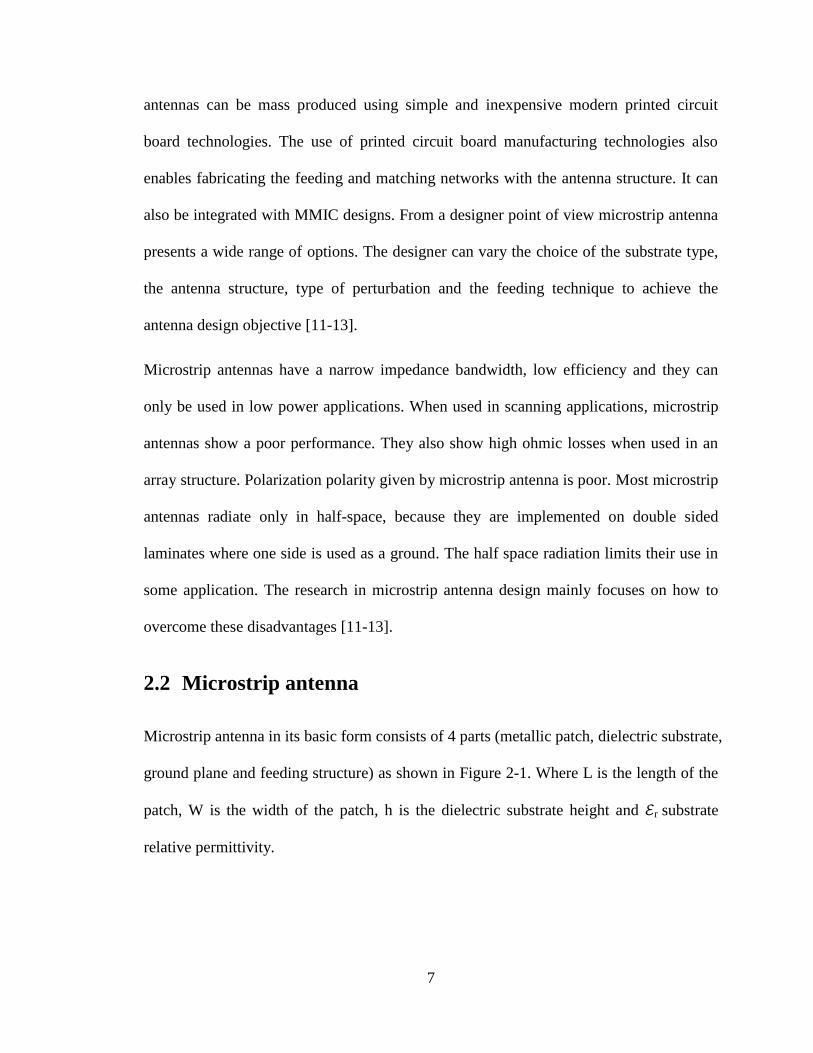
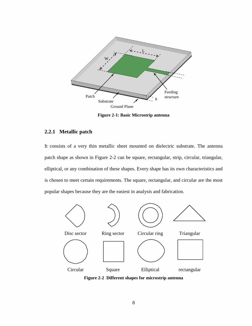
Microstrip antenna in its basic form consists of 4 parts (metallic patch, dielectric substrate,

ground plane and feeding structure) as shown in Figure 2-1. Where L is the length of the

patch, W is the width of the patch, h is the dielectric substrate height and ℰr substrate

relative permittivity.

8

Figure ‎2-1: Basic Microstrip antenna

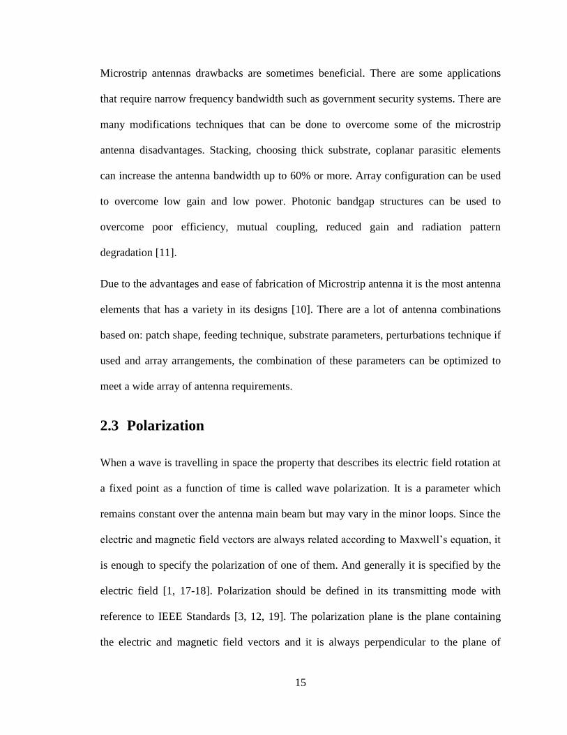
2.2.1 Metallic patch

It consists of a very thin metallic sheet mounted on dielectric substrate. The antenna

patch shape as shown in Figure 2-2 can be square, rectangular, strip, circular, triangular,

elliptical, or any combination of these shapes. Every shape has its own characteristics and

is chosen to meet certain requirements. The square, rectangular, and circular are the most

popular shapes because they are the easiest in analysis and fabrication.

Disc sector Ring sector Circular ring Triangular

Circular Square Elliptical rectangular

Figure ‎2-2 Different shapes for microstrip antenna

W

L

h Substrate

Ground Plane

Patch Feeding

structure

9

2.2.2 Dielectric substrate

It is the dielectric layer between the patch and the ground. There are a lot of substrate

material and specifications to choose from according to the antenna requirement. The

most two factors specifying dielectric substrate is substrate height (0.003 λ ≤h λ )

and dielectric constant (2.2 ≤ ℰr ≤ 12) As ℰr gets higher in value the antenna size

gets smaller.

Substrates that are thick with low dielectric constant are preferable for enhancing

efficiency, bandwidth and radiation in space. On the other hand substrates that are thin

with high dielectric constant are preferable for microwave circuits.

2.2.3 The ground

It is the metallic part found on the other side of the substrate. There are some

perturbations that can be done to the ground to enhance the antenna performance towards

certain specifications, like inserting shapes or slots in the ground plane [11, 14-15].

2.2.4 Feeding

The most four popular feeding techniques for microstrip patch antenna are: (coaxial

feeding, microstrip feeding, proximity feeding and aperture feeding).

2.2.4.1 Coaxial feeding

It is one of the basic techniques used in feeding microwave power. The coaxial cable is

connected to the antenna such that its outer conductor is attached to the ground plane

while the inner conductor is soldered to the metal patch [1, 11-12].

10

Figure ‎2-3 Coaxial feeding

Coaxial feeding is simple to design, easy to fabricate, easy to match and have low

spurious radiation [11-12]. However coaxial feeding has the disadvantages of requiring

high soldering precision. There is difficulty in using coaxial feeding with an array since a

large number of solder joints will be needed. Coaxial feeding usually gives narrow

bandwidth and when a thick substrate is used a longer probe will be needed which

increases the surface power and feed inductance [11-13].

2.2.4.2 Microstrip feeding

In microstrip feed, the patch is fed by a microstrip line that is located on the same plane

as the patch. In this case both the feeding and the patch form one structure. Microstrip

feeding is simple to model, easy to match and easy to fabricate. It is also a good choice

for use in antenna-array feeding networks. However microstrip feed has the disadvantage

of narrow bandwidth and the introduction of coupling between the feeding line and the

patch which leads to spurious radiation and the required matching between the microstrip

patch and the 50 feeding line. Microstrip feed can be classified into 3 categories:

11

Direct feed: where the feeding point is on one edge of the patch. As shown in Figure 2-4.

Direct feed needs a matching network between the feed line and the patch (such as

quarter wavelength transformer). The Quarter wave length transformer compensates the

impedance differences between the patch and the 50 feed line. The quarter wave length

transformer is calculated according to formulas found in [12, 16].

Figure ‎2-4 Direct microstrip feed line

Inset feed: where the feeding point is inside the patch. The location of the feed is the

same that will be used for coaxial feed. The 50 feed line is surrounded with an air gap

till the feeding point as shown in Figure 2-5 . The inset microstrip feeding technique is

more suitable for arrays feeding networks [11-13].

Gap-coupled: the feeding line does not contact the patch; there is an air gap between the

50 line and the patch as shown in Figure 2-6 .The antenna is fed by coupling between

the 50 feed line and the patch.

L

W

Wf

Ltr

Wtr

L Patch length,

W Patch length,

Wf 50 feed line width

Ltr Quarter wave length

transformer length

Wtr Quarter wave length

transformer Width

12

Figure ‎2-5 Inset microstrip feed line

Figure ‎2-6 Gap-coupled microstrip feed line

2.2.4.3 Proximity coupled feeding

Proximity coupled feeding consists of two dielectric substrate layers. The microstrip

patch antenna is located on the top of the upper substrate & the microstrip feeding line is

located on the top of the lower substrate as shown in Figure 2-7. It is a non contacting

feed where the feeding is conducted through electromagnetic coupling that takes place

between the patch and the microstrip line. The two substrates parameters can be chosen

different than each other to enhance antenna performance [11, 13]. The proximity

W

L

Wg

L Patch length,

W Patch length,

Wf feed line width

Wg Air gap Width

Wf

L

W

Wf

l

w

L Patch length,

W Patch length,

Wf feed line width

l Inset Depth

w Inset separation from

patch

13

coupled feeding reduces spurious radiation and increase bandwidth. However it needs

precise alignment between the 2 layers in multilayer fabrication.

Figure ‎2-7 Proximity coupled microstrip feeding

2.2.4.4 Aperture – coupled feeding

Aperture coupled feeding consists of two substrate layers with common ground plane in-

between the two substrates , the microstrip patch antenna is on the top of the upper

substrate & the microstrip feeding line on the bottom of the lower substrate and there is a

slot cut in the ground plane as shown in Figure 2-8. The slot can be of any size or shape

and is used to enhance the antenna parameters. It is a non contacting feed; the feeding is

done through electromagnetic coupling between the patch and the microstrip line through

the slot in the ground plane. The two substrates parameters can be chosen different than

each other to enhance antenna performance [1-2, 11-13]. The aperture feeding reduces

spurious radiation. It also increases the antenna bandwidth, improves polarization purity

Patch

Upper Substrate

Feed line

Lower Substrate

Ground

(a) Microstrip Patch (b) Cross Section In patch

14

and reduces cross-polarization. But it has the same difficulty of the aperture feeding

which is the multilayer fabrication.

Figure ‎2-8 Aperture coupled microstrip feed

2.2.5 Methods of analysis

Due to the attention given to the microstrip antenna and the importance to understand its

physical insight there are many methods to analyze microstrip antennas. Among these

methods, Transmission-line model: it is the simplest and easiest model. It gives good

physical insight. However it is not versatile, less accurate and difficult in modeling

coupling [11, 13]. Cavity model: it is more complex than the transmission-line model and

also difficult in modeling coupling. However it is more accurate and gives more physical

insight [11, 13]. Full wave: it is the most accurate and versatile model, it can be applied

to any microstrip antenna structure. However it is very complex and gives less physical

insight [11, 13].

Patch

Upper Substrate

Feed line

Lower Substrate

Ground

Ground Slot

(a) Microstrip patch (b) Cross section in patch

15

Microstrip antennas drawbacks are sometimes beneficial. There are some applications

that require narrow frequency bandwidth such as government security systems. There are

many modifications techniques that can be done to overcome some of the microstrip

antenna disadvantages. Stacking, choosing thick substrate, coplanar parasitic elements

can increase the antenna bandwidth up to 60% or more. Array configuration can be used

to overcome low gain and low power. Photonic bandgap structures can be used to

overcome poor efficiency, mutual coupling, reduced gain and radiation pattern

degradation [11].

Due to the advantages and ease of fabrication of Microstrip antenna it is the most antenna

elements that has a variety in its designs [10]. There are a lot of antenna combinations

based on: patch shape, feeding technique, substrate parameters, perturbations technique if

used and array arrangements, the combination of these parameters can be optimized to

meet a wide array of antenna requirements.

2.3 Polarization

When a wave is travelling in space the property that describes its electric field rotation at

a fixed point as a function of time is called wave polarization. It is a parameter which

remains constant over the antenna main beam but may vary in the minor loops. Since the

electric and magnetic field vectors are always related according to Maxwell’s equation, it

is enough to specify the polarization of one of them. And generally it is specified by the

electric field [1, 17-18]. Polarization should be defined in its transmitting mode with

reference to IEEE Standards [3, 12, 19]. The polarization plane is the plane containing

the electric and magnetic field vectors and it is always perpendicular to the plane of

16

propagation [1, 20]. The contour drawn by the tip of the electric field vector describes the

wave polarization. This contour is an ellipse, circle or a line [1]. The polarization

direction is assumed in the direction of the main beam unless otherwise stated [12].

There are 2 kinds of polarization co-and cross-polarizations. Co-polarization is the

polarization radiated/received by the antenna, while the cross-polarization is

perpendicular to it [12].

Polarization is a very important factor in wave propagation between the transmitting and

receiver antennas. Having the same kind of polarization and sense is important so that the

receiving antenna can extract the signal from the transmitted wave [21]. Maximum power

transfer will take place when the receiving antenna has the same direction, axial ratio,

spatial orientation and the same sense of polarization as incident wave, otherwise there

will be polarization mismatch. If polarization mismatch occurs it will add more losses [1-

3, 12]. Polarization is very important when considering wave reflection [17].

2.3.1 Types of polarization

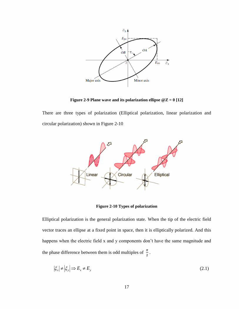
The shape of the contour drawn by the tip of the electric field vector is called the

polarization ellipse. This ellipse describes everything in polarization as shown in

Figure 2-9.

Axial ratio states the shape of the polarization ellipse. Tilt angle states its orientation. The

direction of the electric field vector is the sense of polarization in the direction of

propagation [1].

17

Figure ‎2-9 Plane wave and its polarization ellipse @Z = 0 ‎[12]

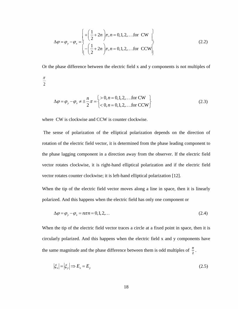
There are three types of polarization (Elliptical polarization, linear polarization and

circular polarization) shown in Figure 2-10

Figure ‎2-10 Types of polarization

Elliptical polarization is the general polarization state. When the tip of the electric field

vector traces an ellipse at a fixed point in space, then it is elliptically polarized. And this

happens when the electric field x and y components don’t have the same magnitude and

the phase difference between them is odd multiples of

.

x y x yE E (2.1)

18

12 , 0,1,2, .for CW

2

12 , 0,1,2, .for CCW

2

y x

n n

n n

(2.2)

Or the phase difference between the electric field x and y components is not multiples of

2

0, 0,1,2, .for CW

0, 0,1,2, .for CCW2y x

nn

n

(2.3)

where CW is clockwise and CCW is counter clockwise.

The sense of polarization of the elliptical polarization depends on the direction of

rotation of the electric field vector, it is determined from the phase leading component to

the phase lagging component in a direction away from the observer. If the electric field

vector rotates clockwise, it is right-hand elliptical polarization and if the electric field

vector rotates counter clockwise; it is left-hand elliptical polarization [12].

When the tip of the electric field vector moves along a line in space, then it is linearly

polarized. And this happens when the electric field has only one component or

0,1,2,y x n n (2.4)

When the tip of the electric field vector traces a circle at a fixed point in space, then it is

circularly polarized. And this happens when the electric field x and y components have

the same magnitude and the phase difference between them is odd multiples of

.

x y x yE E (2.5)

19

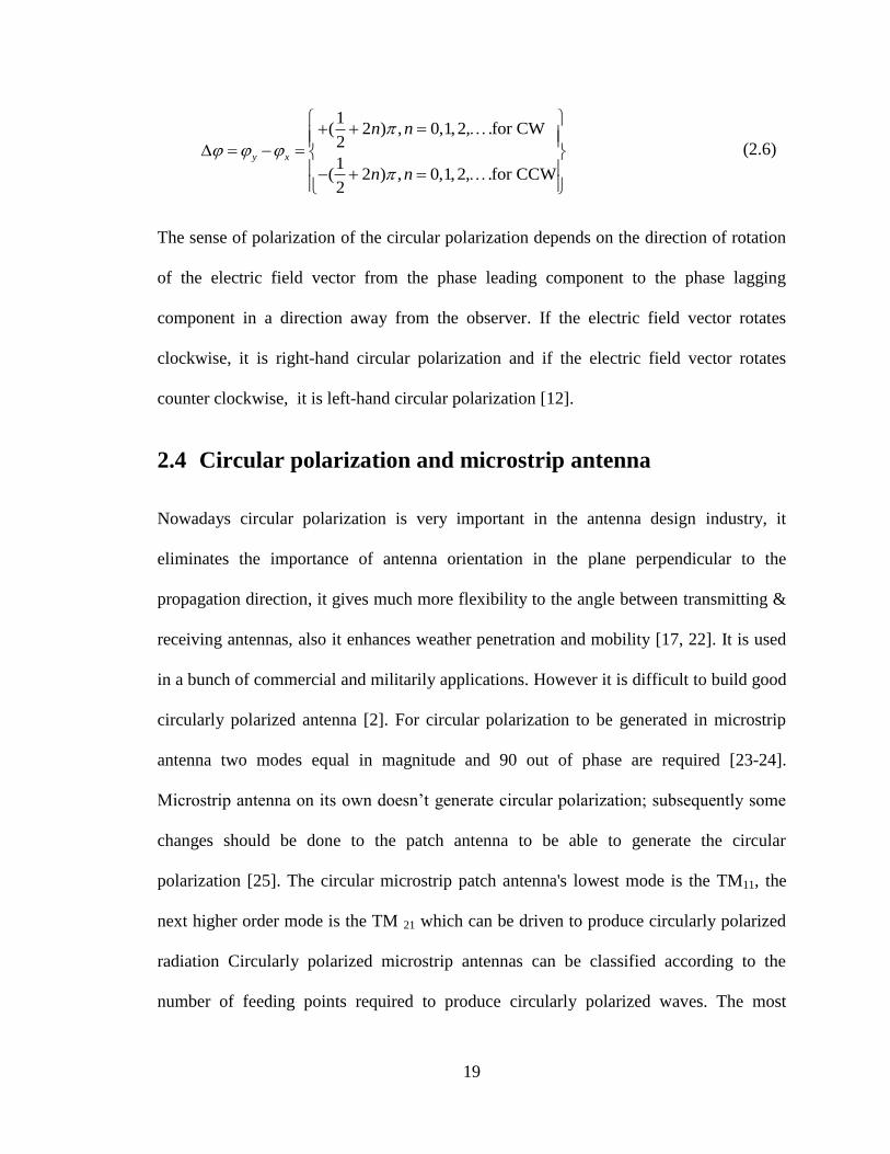
1( 2 ) , 0,1,2, .for CW2

1( 2 ) , 0,1,2, .for CCW2

y x

n n

n n

(2.6)

The sense of polarization of the circular polarization depends on the direction of rotation

of the electric field vector from the phase leading component to the phase lagging

component in a direction away from the observer. If the electric field vector rotates

clockwise, it is right-hand circular polarization and if the electric field vector rotates

counter clockwise, it is left-hand circular polarization [12].

2.4 Circular polarization and microstrip antenna

Nowadays circular polarization is very important in the antenna design industry, it

eliminates the importance of antenna orientation in the plane perpendicular to the

propagation direction, it gives much more flexibility to the angle between transmitting &

receiving antennas, also it enhances weather penetration and mobility [17, 22]. It is used

in a bunch of commercial and militarily applications. However it is difficult to build good

circularly polarized antenna [2]. For circular polarization to be generated in microstrip

antenna two modes equal in magnitude and 90 out of phase are required [23-24].

Microstrip antenna on its own doesn’t generate circular polarization; subsequently some

changes should be done to the patch antenna to be able to generate the circular

polarization [25]. The circular microstrip patch antenna's lowest mode is the TM11, the

next higher order mode is the TM 21 which can be driven to produce circularly polarized

radiation Circularly polarized microstrip antennas can be classified according to the

number of feeding points required to produce circularly polarized waves. The most

20

commonly used feeding techniques in circular polarization generation are dual feed and

single feed [24].

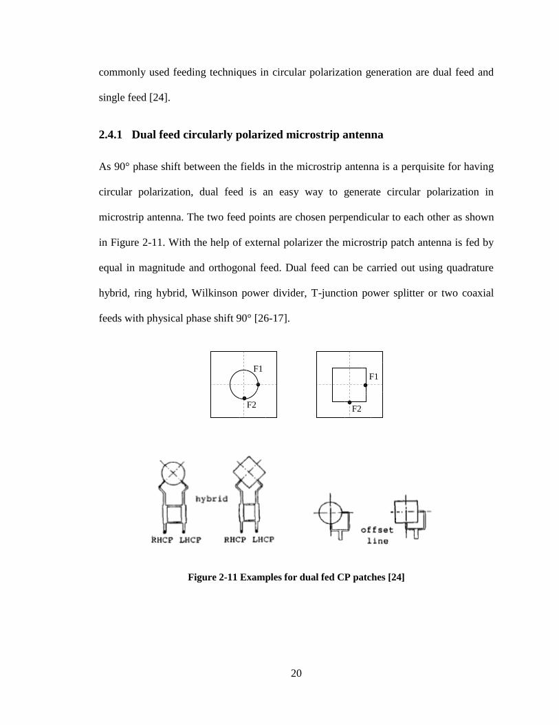
2.4.1 Dual feed circularly polarized microstrip antenna

As 90° phase shift between the fields in the microstrip antenna is a perquisite for having

circular polarization, dual feed is an easy way to generate circular polarization in

microstrip antenna. The two feed points are chosen perpendicular to each other as shown

in Figure 2-11. With the help of external polarizer the microstrip patch antenna is fed by

equal in magnitude and orthogonal feed. Dual feed can be carried out using quadrature

hybrid, ring hybrid, Wilkinson power divider, T-junction power splitter or two coaxial

feeds with physical phase shift 90° [26-17].

Figure ‎2-11 Examples for dual fed CP patches ‎[24]

F1

F2

F1

F2

21

2.4.2 Single feed circularly polarized microstrip antenna

Single fed microstrip antennas are simple, easy to manufacture, low cost and compact in

structure as shown in Figure 2-12. It eliminates the use of complex hybrid polarizer,

which is very complicated to be used in antenna array [24, 28]. Single fed circularly

polarized microstrip antennas are considered to be one of the simplest antennas that can

produce circular polarization [7]. In order to achieve circular polarization using only

single feed two degenerate modes should be exited with equal amplitude and 90°

difference. Since basic shapes microstrip antenna produce linear polarization there must

be some changes in the patch design to produce circular polarization. Perturbation

segments are used to split the field into two orthogonal modes with equal magnitude and

90° phase shift. Therefore the circular polarization requirements are met.

Figure ‎2-12 single fed patches

The dimensions of the perturbation segments should be tuned until it reach an optimum

value at the design frequency [24, 27, 29-30].

Single feeding techniques previously discussed in section 2.1.4.

22

2.5 Single fed circularly polarized microstrip antenna

Single feeding techniques are very common with microstrip antennas as they are simple,

easy to manufacture, low in cost and compact in structure.

Several techniques were used to achieve circular polarization in single fed microstrip

antenna. Among these techniques: fractal boundary [22, 31-35], square patch with shaped

slots [7, 36, 38], embedding cross slot in metallic patch or the ground plane [38], staking

antennas [30, 39], annular ring with stripline inside the inner ring [23], and truncated

edges patches [4, 40].

2.5.1.1 Square patch with shaped slots

Cutting a slot in a microstrip patch antenna gives the perturbation needed to produce

circular polarization. The shape and the dimensions of the cut out slot also widen the

bandwidths [27, 36, 37].

2.5.1.1.1 C-shaped slot

Cutting C-shaped slot in a square patch microstrip antenna as shown in Figure 2-13 and

mounting the substrate on a foam layer good circular polarization is achieved. The

antenna structure is fed using aperture coupling feeding method. The dimensions of the

slot are used to optimize the antenna design in the favour of axial ratio and impedance

matching. The measured 3 dB axial ratio and 10 dB impedance bandwidths are 3.1 % and

16.4 % respectively [36].

23

Figure ‎2-13 Microstrip square patch antenna with C-shaped slot ‎[36]

2.5.1.1.2 F-shaped slot

Cutting F-shaped slot in the center of a square patch as shown in Figure 2-14 and fed

with aperture coupling. Good circular polarization with 3 dB axial ratio and 10 dB

impedance bandwidths are 3.2 % and 5.62 % respectively [7].

Figure ‎2-14 Microstrip square patch antenna with F-shaped slot ‎[7]

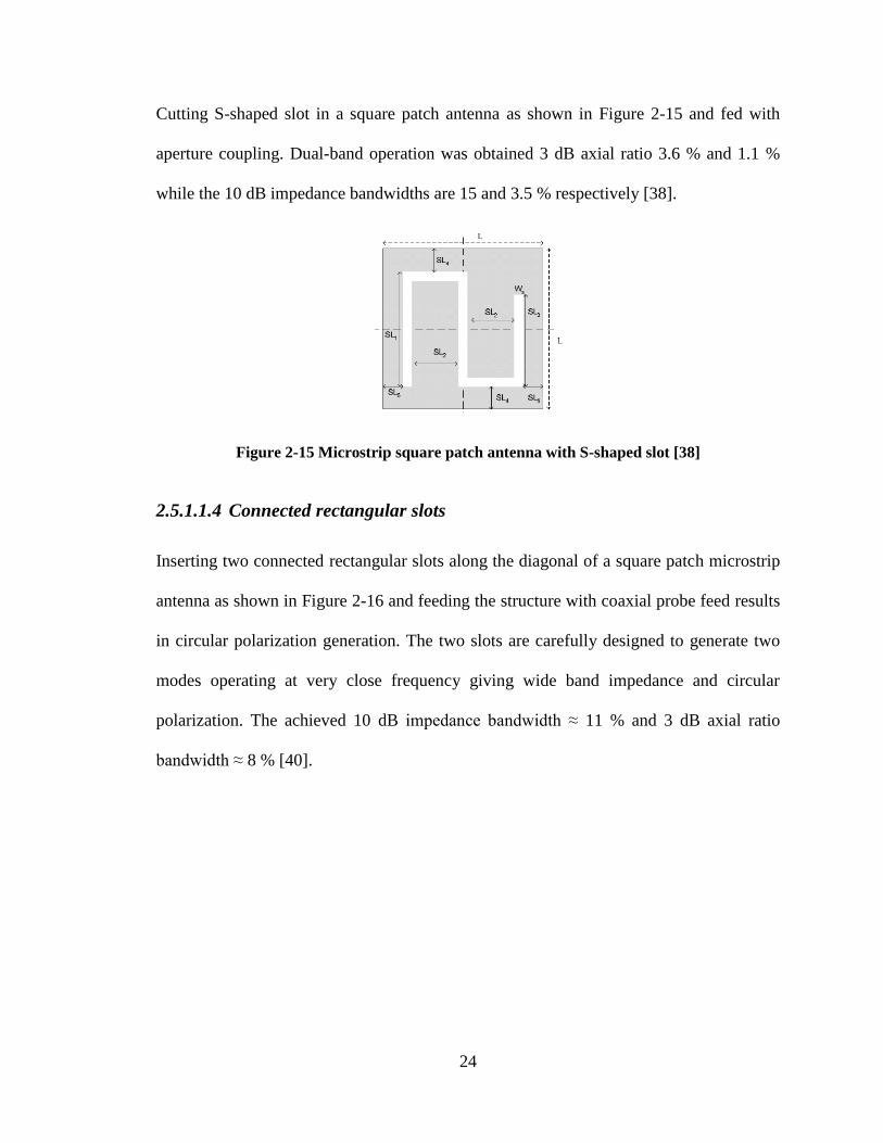
2.5.1.1.3 S-shaped slot

24

Cutting S-shaped slot in a square patch antenna as shown in Figure 2-15 and fed with

aperture coupling. Dual-band operation was obtained 3 dB axial ratio 3.6 % and 1.1 %

while the 10 dB impedance bandwidths are 15 and 3.5 % respectively [38].

Figure ‎2-15 Microstrip square patch antenna with S-shaped slot ‎[38]

2.5.1.1.4 Connected rectangular slots

Inserting two connected rectangular slots along the diagonal of a square patch microstrip

antenna as shown in Figure 2-16 and feeding the structure with coaxial probe feed results

in circular polarization generation. The two slots are carefully designed to generate two

modes operating at very close frequency giving wide band impedance and circular

polarization. The achieved 10 dB impedance bandwidth ≈ 11 % and 3 dB axial ratio

bandwidth ≈ 8 % [40].

25

Figure ‎2-16 Microstrip square patch antenna with 2 connected rectangular slots ‎[40]

2.5.1.2 Cross slot

By inserting a cross slot in a circular patch antenna as shown in Figure 2-17 circularly

polarized compact size antenna is obtained. Optimizing the cross slot dimensions and the

ratio between the two arms affects the axial ratio, impedance bandwidths and the antenna

size dramatically. Increasing the slot length will decrease the resonant frequency hence

decreasing the antenna size. The antenna is fed by proximity feed and when tested the

antenna radius was 36 % smaller than antenna without the cross slot [38].

Figure ‎2-17 Circular patch with cross slot

The microstrip antenna with large cross slot lengths will have decreased operating

frequency. But the cross slot ratio is mainly determined by the slot length, so the ratio

will be close to 1 which will be difficult in fabrication. Embedding an additional equal

arm cross slot in the ground plane as shown in Figure 2-18 more compact size antenna

26

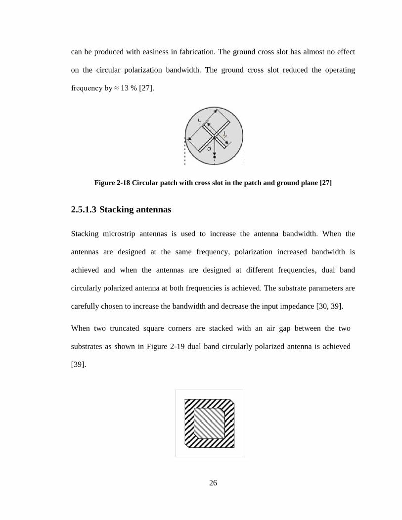
can be produced with easiness in fabrication. The ground cross slot has almost no effect

on the circular polarization bandwidth. The ground cross slot reduced the operating

frequency by ≈ 13 % [27].

Figure ‎2-18 Circular patch with cross slot in the patch and ground plane ‎[27]

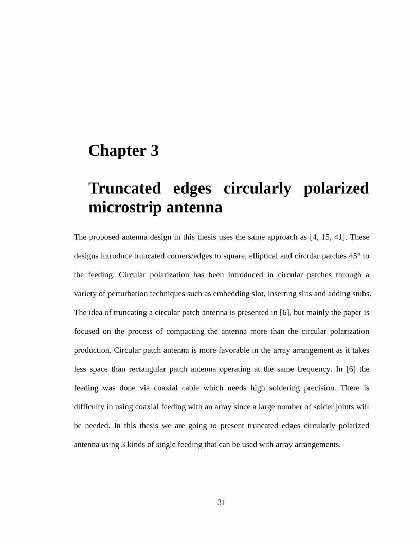
2.5.1.3 Stacking antennas

Stacking microstrip antennas is used to increase the antenna bandwidth. When the

antennas are designed at the same frequency, polarization increased bandwidth is

achieved and when the antennas are designed at different frequencies, dual band

circularly polarized antenna at both frequencies is achieved. The substrate parameters are

carefully chosen to increase the bandwidth and decrease the input impedance [30, 39].

When two truncated square corners are stacked with an air gap between the two

substrates as shown in Figure 2-19 dual band circularly polarized antenna is achieved

[39].

27

Figure ‎2-19 Stacked truncated corners square patches

When stacking a nearly square patch over a nearly square ring as shown in Figure 2-20

good circular polarization is excited. There is a foam layer inserted between the two

substrates to help increase the bandwidth. The lower layer is fed diagonally with a

coaxial cable and the upper layer is fed by proximity coupling from the lower layer. The

3 dB axial ratio bandwidth is ≈ 18.85 % and impedance bandwidth ≈ 22.13 % the circular

polarization quality is excellent over the entire hemisphere [30].

Figure ‎2-20 Stacked square patch over square ring ‎[30]

2.5.1.4 Truncated edges patches

Truncated corners square microstrip patch antenna is among the first and most famous

basic techniques to generate circular polarization in patch antennas. The open literature is

very rich with truncated corners square microstrip antenna [4, 15, 41]. Inserting 4 equal

length slits at the 4 corners of truncated corners square microstrip patch antenna as shown

in Figure 2-21 gives a compact circularly polarized antenna. The size reduction is ≈ 36 %

than the patch without the 4 slits [4].

28

Figure ‎2-21 Truncated corner square microstrip antenna with 4 slits ‎[4]

Truncated edges elliptical antenna, where opposite edges of the elliptical antenna parallel

to the major axis are truncated as shown in Figure 2-22. The antenna results in circular

polarization higher than the conventional elliptical antenna with 10 dB impedance

bandwidth 5.7 % and 3 dB axial ratio bandwidth 1.45 %.

Figure ‎2-22 Truncated edges elliptical antenna ‎[5]

When truncating peripheral edges from circular antenna with embedded cross slot and fed

with coaxial cable as shown in Figure 2-23 produces compact circular polarization

antenna [6].

29

Figure ‎2-23 Truncated edges circular microstrip antenna ‎[6]

2.5.1.5 Annular ring with stripline inside the inner ring

Inserting a strip line in the inner circle of an annular ring as shown in Figure 2-24 results

in a compact circularly polarized microstrip antenna. The strip line is 45° to the feed and

it also help in the antenna size reduction. The resonant frequency will decrease with

decreasing the strip line width [23].

Figure ‎2-24 Annular ring with inner strip line ‎[23]

2.6 Summary

This chapter discussed the components of microstrip antenna, its feeding techniques and

methods of analysis. We also revised wave polarization, its kinds and its importance. The

30

use of circularly polarized antennas presents an attractive solution to achieve this

polarization match. Microstrip antenna is the most popular antenna in circular

polarization generation. Circular polarization can be achieved in microstrip antenna by

either using dual feed or by using perturbation segment with single feed.

31

Chapter 3

Truncated edges circularly polarized

microstrip antenna

The proposed antenna design in this thesis uses the same approach as [4, 15, 41]. These

designs introduce truncated corners/edges to square, elliptical and circular patches 45° to

the feeding. Circular polarization has been introduced in circular patches through a

variety of perturbation techniques such as embedding slot, inserting slits and adding stubs.

The idea of truncating a circular patch antenna is presented in [6], but mainly the paper is

focused on the process of compacting the antenna more than the circular polarization

production. Circular patch antenna is more favorable in the array arrangement as it takes

less space than rectangular patch antenna operating at the same frequency. In [6] the

feeding was done via coaxial cable which needs high soldering precision. There is

difficulty in using coaxial feeding with an array since a large number of solder joints will

be needed. In this thesis we are going to present truncated edges circularly polarized

antenna using 3 kinds of single feeding that can be used with array arrangements.

32

This chapter presents in details, the design methodology and steps used to design a

truncated edges circularly polarized microstrip antenna. The antenna is fed by three 3

different types of single feeding (microstrip line, proximity and aperture)

3.1 Design methodology

The first stage is designing a perfect circular patch antenna operating at 2.4 GHz and its

feeding network according to the type of feeding used. After determining the radius,

introducing the perturbation technique then takes place. A parametric study for choosing

antenna radius, the dimensions of the perturbation segments and the other antenna

parameters such as the ground slot dimensions in the aperture feeding are presented

explaining the chosen parameters.

3.2 Truncated edges circularly polarized antenna

The proposed antennas are based on a circular microstrip antenna. Equation (3.1) gives

an initial value for the radius of a circular microstrip antenna to operate at 2.4 GHz.

1

221 ln 1.7726

2r

Frad

h F

F h

(3.1)

where

98.791 10

r r

Ff

(3.2)

33

rad = the patch radius, fr = design frequency, and h = the dielectric substrate height .The

substrate used is (RT/duroid 5880) with height h = 1.57 mm and ℰr = dielectric constant

= 2.2.

Using Equation (3.1) the antenna initial radius calculated for a perfect circular microstrip

antenna operating at 2.4 GHz is equal to 23.6 mm. After determining the radius the

feeding network is designed according to the type of feeding used as will be discussed in

details in section 3.3, section 3.4 and section 3.5. In order to achieve circular polarization

perturbation segment should be used for the generation of the two degenerate modes. In

this thesis the perturbation used is to truncate two opposite edges of a circular patch with

45° angle to the feed line. Introducing these truncates will affect the antenna design

parameters which may lead to changes in the calculated results such as the patch radius

and the centre frequency. As will be shown later the distance between the patch centre

and the perturbation segments (d) is responsible for circular polarization generation.

One of the major problems in circular polarization generation is having the best return

loss and the best axial ratio at different frequencies. Antenna parameters were chosen

such that to give acceptable return loss and axial ratio at the design frequency.

This thesis focuses on comparing three single feeding techniques microstrip feeding,

proximity feeding, and aperture feeding. A comparison is done in terms of the axial ratio,

the return loss and the radiation patterns resulting from the use of each feeding technique.

3.3 Microstrip feeding

The microstrip feed consists of a 50 transmission line connected to the patch through a

quarter wave length transformer to compensate the impedance difference between the

34

patch antenna and the 50 line as shown in Figure 3-1. First determining the value of

perfect circular patch radius (rad) using Equation (3.1). The width of the 50 line is

determined using Equation (3.3).

Figure ‎3-1 Antenna with microstrip feed

2

8   1.52

2  

  12 0.611 2 1 1 0.39 1.52

2   

A

A

l

r

r r

heA

ew

hB ln B ln B A

(3.3)

12  1   1 0.11

A 0.2360 2 1  

o r r

r r

Z

(3.4)

2

0

60 B

Z

(3.5)

The calculated width of the feed line is 4.9 mm, but usually calculations give a starting

point. The feed line width calculation is refined using Rogers Corporation computer aided

program MWI-2010 [43] and the feed line width is 4.88 mm. Using HFSS a perfect

Ltr

Wtr

Wf

rad d

35

circle radius 23.6 mm and fed directly with 50 with width (Wf) = 4.88 mm is

simulated to determine the antenna impedance which is 375 . To design the quarter

wave length transformer its impedance has to be determined using Equation (3.6).

Quarter wave length transformer  (       )patchimpedance Z (3.6)

The quarter wave length transformer impedance is 137 and its calculated width using

Equation (3.3) is 0.63 mm.

eff

The length of the quarter wave length transformer= / 4 (3.7)

λeff = λo/ eff ,where λeff is the effective wavelength, λo is free space wave length;

eff is the effective substrate dielectric constant. According to Rogers Corporation MWI-

2010 [43] the width of quarter wave length transformer is 0.61 mm, the effective

wavelength = 95 mm and effective dielectric constant = 1.7494.

The circular patch antenna with the above mentioned dimensions resonates at 2.43 GHz.

Since the antenna radius controls the antenna operating frequency, tweaking the antenna

radius until the antenna operates at 2.4 GHz. The antenna radius and the frequency are

inversely proportional, so the radius has to be increased till the resonance frequency is 2.4

GHz. A parametric study is carried out to determine the perfect circle radius. As shown in

Figure 3-2 the radius that makes the antenna resonate at 2.4 GHz is 23.96 mm.

36

Figure ‎3-2 Perfect circle radius parametric study - microstrip feeding

When introducing the perturbation, another parametric study is performed to determine

the optimum distance between the patch centre and the perturbation segments (d). The

results of this parametric study the effect of changing (d) on the antenna return loss and

axial ratio will be shown in Figure 3-3, Figure 3-4 and Figure 3-5 .

The distance (d) is chosen to give the most acceptable axial ratio and return loss at the

design frequency. As shown in Figure 3-3 the best return loss and axial ratio at 2.4 GHz

occurs at (d) = 23 mm, and (d) = 22.6 mm respectively. As shown in Figure 3-4 as (d)

increases there are 2 modes getting closer to each other near the design frequency. As

shown in Figure 3-3 with increasing (d) the axial ratio value increase till (d) = 22.6 mm it

starts to decrease again and the return loss increases with increasing the value of (d). The

2.3 2.35 2.4 2.45 2.5-30

-25

-20

-15

-10

-5

0

Frequency GHz

Re

turn

lo

ss d

B

23.6mm

23.8mm

23.9mm

23.96mm

24mm

24.1mm

37

value of (d) is chosen to be 22.6 mm. Even though much lower return loss can be

achieved at higher values for (d), but the antenna at this stage is not matched yet. Further

enhancement for the return loss at (d) = 22.6 mm is expected after matching, but nothing

is expected to further enhance the axial ratio. After choosing the antenna radius (rad) and

the perturbation distance value (d), with the help of HFSS the antenna new impedance is

determined and a new quarter wave length transformer is designed.

(i)Retrun loss versus (d) (ii) Axial ratio versus (d)

Figure ‎3-3 Parametric analysis of (d) at 2.4 GHz - microstrip feeding

The first antenna fed with microstrip line feed parameters are, (rad) = 23.96 mm, the

length of the quarter wavelength transformer (Ltr) = eff

/ 4 = 23.5 mm, and its width

(Wtr) = 1.15 mm, the distance between the perturbation segment and the patch center (d)

= 22.6 mm, and the width of the 50 line (Wf) = 4.88 mm. Antenna results will be

shown in section 4.3.1.

22 22.1 22.2 22.3 22.4 22.5 22.6 22.7 22.8 22.9 23-25

-20

-15

-10

-5

Perturbation distance from the patch center (d) mm

Re

tru

n lo

ss d

B

22 22.2 22.4 22.6 22.8 230

1

2

3

4

5

6

7

Perturbation distance from patch center (d)

Axia

l ra

tio

dB

38

Figure ‎3-4 Return loss for (d) parametric study - microstrip feeding

Figure ‎3-5 Axial ratio for (d) parametric study - microstrip feeding

2.3 2.35 2.4 2.45 2.5-30

-25

-20

-15

-10

-5

0

Frequency GHz

Re

turn

lo

ss d

B

22mm

22.2mm

22.5mm

22.6mm

22.7mm

22.8mm

23mm

2.35 2.4 2.450

5

10

15

Frequency GHz

Axia

l ra

tio

dB

22mm

22.2mm

22.5mm

22.6mm

22.7mm

22.8mm

23mm

39

3.4 Proximity feeding

The two substrates used in the proximity feeding here are the same for the antenna and

the feed. The patch is located on the top of the upper substrate with no ground and the

feed line is located on the top of the lower substrate with ground as shown in Figure 3-6.

As been done in section 3.3, the initial value for perfect antenna radius is calculated using

Equation (3.1) (rad) = 23.6 mm. The calculations for the microstrip feeding showed that

the calculated width of the 50 feed line is 4.9 mm, but verifying this value using HFSS

the line width with 50 impedance to be used with the proximity feeding is 4.62 mm.

Figure ‎3-6 3D view for proximity fed antenna

A perfect circular patch antenna with the above mentioned dimensions as shown in

Figure 3-7 resonate at 2.39 GHz, since the antenna radius controls the antenna operating

frequency and the antenna radius is inversely proportional to the frequency; the antenna

radius needs to be decreased. A very narrow ranged parametric study is performed as

shown in Figure 3-8 to determine the perfect circle radius at 2.4 GHz. The optimum

antenna radius is 23.44 mm.

When introducing the perturbation a parametric study is performed to determine the

optimum distance between the patch centre and the perturbation segments (d). The results

40

of this parametric study and the effect of changing (d) on the antenna return loss and axial

ratio are shown in Figure 3-10, Figure 3-11and Figure 3-9. The distance (d) is chosen to

give the most acceptable axial ratio and return loss at the design frequency.

Figure ‎3-7 Antenna fed by proximity feeding

Figure ‎3-8 Perfect circle radius parametric study - proximity feeding

2.3 2.35 2.4 2.45 2.5-14

-12

-10

-8

-6

-4

-2

Frequency GHz

Re

turn

lo

ss d

B

23.4mm

23.44mm

23.5mm

23.6mm

23.7mm

Lf

d

rad Wf

41

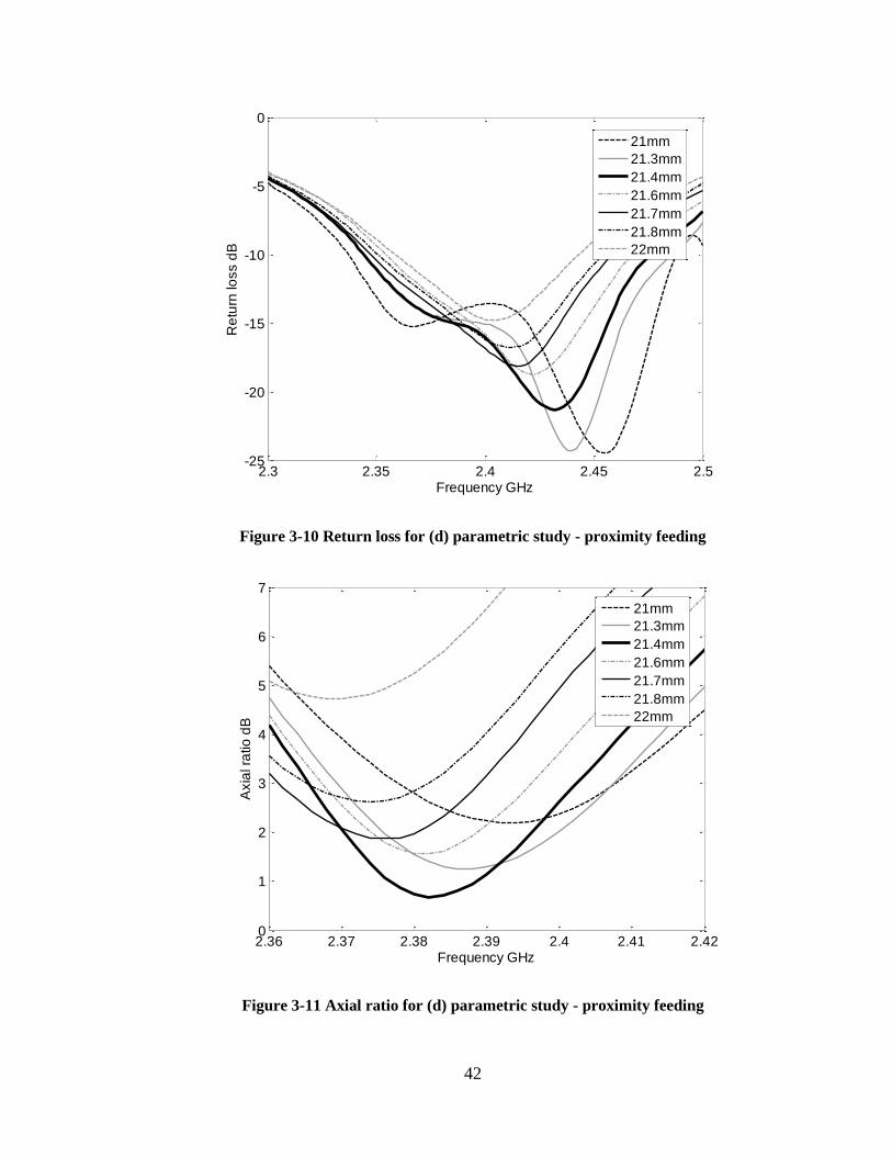
Figure 3-9 shows that the best return loss and axial ratio at 2.4 GHz occurs at (d) = 21.7

mm, and (d) = 21.3 mm respectively. Regarding Figure 3-10 and Figure 3-11 the value of

(d) is chosen to be 21.4 mm. Even though 21.3 mm gives better axial ratio at 2.4 GHz,

but considering Figure 3-11 (d) = 21.4 mm better return loss at 2.4 GHz and minimum

axial ratio at 2.38 GHz which can shift to 2.4GHz after determining the length of the

feed line or by decreasing the antenna radius .

Figure 3-10 shows that as (d) increases there are 2 modes getting closer to each other near

the design frequency.

After determining the antenna radius (rad) and the perturbation distance value (d), a new

parametric study is performed to choose the length of the feed line (Lf).

(i)Retrun loss versus (d) (ii) Axial ratio versus (d)

Figure ‎3-9 Parametric analysis of (d) at 2.4 GHz - proximity feeding

20.5 20.7 20.9 21.1 21.3 21.5 21.7 21.922-18

-16

-14

-12

-10

-8

Perturbation distance from patch center (d) mm

Re

turn

lo

ss d

B

20.5 20.7 20.9 21.1 21.3 21.5 21.7 21.9220

1

2

3

4

5

6

7

Perturbation distance from patch center (d) mm

Axia

l ra

tio

dB

42

Figure ‎3-10 Return loss for (d) parametric study - proximity feeding

Figure ‎3-11 Axial ratio for (d) parametric study - proximity feeding

2.3 2.35 2.4 2.45 2.5-25

-20

-15

-10

-5

0

Frequency GHz

Re

turn

lo

ss d

B

21mm

21.3mm

21.4mm

21.6mm

21.7mm

21.8mm

22mm

2.36 2.37 2.38 2.39 2.4 2.41 2.420

1

2

3

4

5

6

7

Frequency GHz

Axia

l ra

tio

dB

21mm

21.3mm

21.4mm

21.6mm

21.7mm

21.8mm

22mm

43

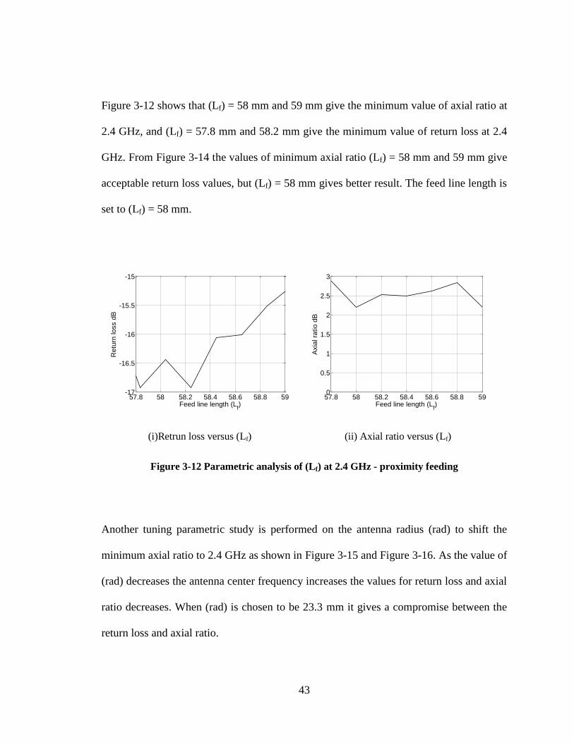
Figure 3-12 shows that (Lf) = 58 mm and 59 mm give the minimum value of axial ratio at

2.4 GHz, and (Lf) = 57.8 mm and 58.2 mm give the minimum value of return loss at 2.4

GHz. From Figure 3-14 the values of minimum axial ratio (Lf) = 58 mm and 59 mm give

acceptable return loss values, but (Lf) = 58 mm gives better result. The feed line length is

set to (Lf) = 58 mm.

(i)Retrun loss versus (Lf) (ii) Axial ratio versus (Lf)

Figure ‎3-12 Parametric analysis of (Lf) at 2.4 GHz - proximity feeding

Another tuning parametric study is performed on the antenna radius (rad) to shift the

minimum axial ratio to 2.4 GHz as shown in Figure 3-15 and Figure 3-16. As the value of

(rad) decreases the antenna center frequency increases the values for return loss and axial

ratio decreases. When (rad) is chosen to be 23.3 mm it gives a compromise between the

return loss and axial ratio.

57.8 58 58.2 58.4 58.6 58.8 59-17

-16.5

-16

-15.5

-15

Feed line length (Lf)

Re

turn

lo

ss d

B

57.8 58 58.2 58.4 58.6 58.8 590

0.5

1

1.5

2

2.5

3

Feed line length (Lf)

Axia

l ra

tio

dB

44

Figure ‎3-13 Return loss for (Lf) parametric study - proximity feeding

Figure ‎3-14 Axial ratio for (Lf) parametric study - proximity feeding

2.36 2.37 2.38 2.39 2.4 2.41 2.42 2.43 2.44 2.45-24

-22

-20

-18

-16

-14

-12

-10

Frequency GHz

Re

turn

lo

ss d

B

57.8mm

58mm

58.2mm

58.8mm

59mm

2.35 2.36 2.37 2.38 2.39 2.4 2.41 2.420

0.5

1

1.5

2

2.5

3

3.5

4

Frequency GHz

Axia

l ra

tio

dB

57.8mm

58mm

58.2mm

58.8mm

59mm

45

Figure ‎3-15 Return loss for re-determining (rad) - proximity feeding

Figure ‎3-16 Axial ratio for re-determining (rad) - proximity feeding

2.35 2.4 2.45 2.5-22

-20

-18

-16

-14

-12

-10

-8

-6

Frequency GHz

Re

tru

n lo

ss d

B

23.2mm

23.25mm

23.3mm

23.44mm

2.35 2.4 2.450

1

2

3

4

5

6

7

Frequency GHz

Axia

l ra

tio

dB

23.2mm

23.25mm

23.3mm

23.44mm

46

After re-determining the radius (rad) another tuning may be needed for (d). Figure 3-17

and Figure 3-18 show that (d) = 21.35 mm gives better results in terms of return loss and

axial ratio at 2.4 GHz. As the value of (d) increases; the value of the return loss

decreases.

The second antenna fed with proximity feeding parameters are, (rad) = 23.3 mm, the

distance between the perturbation segment and the patch center (d) = 21.35 mm, and the

width of the 50 line (Wf) = 4.62 mm. Antenna results will be shown in section 4.3.2.

Figure ‎3-17 Return loss for re-determining (d) - proximity feeding

2.35 2.4 2.45 2.5-20

-18

-16

-14

-12

-10

-8

-6

Frequency GHz

Re

turn

lo

ss d

B

21.3mm

21.35mm

21.4mm

21.45

47

Figure ‎3-18 Axial ratio for re-determining (d) - proximity feeding

3.5 Aperture feeding

The two substrates used in the aperture feeding here are the same for the antenna and the

feed line. The patch is located on the top of the upper substrate, the feed line is located on

the bottom of the lower substrate and there is a common ground plane between the two

substrates as shown in Figure 3-19. There is a slot in the common ground plane. In this

thesis the slot shape is chosen circular to match the metallic patch shape selection.

As done in section 3.3 and section 3.4, the initial value for perfect antenna radius is

calculated using Equation(3.1) (rad) = 23.6 mm. As the calculations for the microstrip

feeding, the calculated width of the 50 feed line is 4.9 mm, but verifying this value

using HFSS the 50 line width to be used with the aperture feeding is 4.36 mm.

2.35 2.4 2.450

1

2

3

4

5

6

7

Frequency GHz

Axia

l ra

tio

dB

21.3mm

21.35mm

21.4mm

24.45mm

48

Figure ‎3-19 3D view for aperture fed antenna

A perfect circular patch antenna with the above mentioned dimensions as shown in

Figure 3-20 resonate at 2.34 GHz. Since the antenna radius controls the antenna operating

frequency and the antenna radius is inversely proportional to the frequency the antenna

radius needs to be decreased. A parametric study is performed as shown in Figure 3-21 to

determine the perfect circle radius at 2.4 GHz. The optimum antenna radius that resonates

at 2.4 GHz is 22.99 mm.

Figure ‎3-20 Antenna fed by aperture feeding

rad d

Lf

Wf

radslot

49

Figure ‎3-21 Perfect circle radius parametric study - aperture feeding

When introducing the perturbation a parametric study is performed to determine the

optimum distance between the patch centre and the perturbation segments (d). The results

of this parametric study and the effect of changing (d) on the antenna return loss and axial

ratio are shown in Figure 3-22. Figure 3-22shows that the best return loss and axial ratio

at 2.4 GHz occurs at (d) = 22 mm, and (d) = 21.5 mm respectively. As shown in

Figure 3-23 as (d) increases there are 2 modes getting closer to each other near the design

frequency. As shown in Figure 3-22 the best value for (d) in terms of axial ratio at

2.4GHz is 21.5 mm, which is not an acceptable value for axial ratio or return loss.

2.3 2.35 2.4 2.45 2.5-30

-25

-20

-15

-10

-5

0

Frequency GHz

Re

turn

lo

ss d

B

22.8mm

22.9mm

23mm

23.5mm

23.6mm

23.7mm

50

(i)Retrun loss versus (d) (ii) Axial ratio versus (d)

Figure ‎3-22 Parametric analysis of (d) at 2.4 GHz - aperture feeding

Also Figure 3-23 and Figure 3-24 show that (d) = 22 mm gives acceptable return loss at

2.4 GHz, but not acceptable value for the axial ratio. At 2.42 GHz some values for (d)

give acceptable axial ratio, but not good return loss at the same value for (d). As a matter

of the fact the antenna is not yet matched and there are still two parametric studies for the

feed line length and the slot radius to be performed. So (d) is chosen to be 21.6 mm as it

has an acceptable axial ratio at 2.42 GHz and the return loss curve minimum occurs at 2.4

GHz.

20 20.5 21 21.5 22-18

-16

-14

-12

-10

-8

-6

-4

-2

Perturbation distance from patch center (d) mm

Re

turn

lo

ss d

B

20 20.5 21 21.5 226

7

8

9

10

11

12

13

14

Perturbation distance from patch center (d) mm

Axia

l ra

tio

dB

51

Figure ‎3-23 Return loss for (d) parametric study - aperture feeding

Figure ‎3-24 Axial ratio for (d) parametric study - aperture feeding

2.35 2.4 2.45 2.5-18

-16

-14

-12

-10

-8

-6

-4

-2

0

Frequency GHz

Re

turn

lo

ss d

B

21mm

21.3mm

21.4mm

21.45mm

21.5mm

21.55m

21.6mm

21.8mm

22mm

2.35 2.4 2.45 2.50

1

2

3

4

5

6

7

8

9

10

Frequency GHz

Axia

l ra

tio

dB

21mm

21.3mm

21.4mm

21.45mm

21.5mm

21.55mm

21.6mm

21.8mm

22mm

52

Weather the effect of the slot radius and the feed line length will improve the axial ratio

and return loss of the antenna at 2.4 GHz or not will be shown in the following

parametric studies.

(i)Retrun loss versus (radslot) (ii) Axial ratio versus (radslot)

Figure ‎3-25 Parametric analysis of (radslot) at 2.4 GHz - aperture feeding

Figure 3-25 shows that changing the radius of the ground plane slot (radslot) affects both

the axial ratio and return loss. The figure also shows that the best values for axial ratio

and return loss at 2.4GHz occurs at (radslot) = 5.5 mm although the value for return loss is

acceptable, but not good. Figure 3-26 shows that when (radslot) = 5.5 mm, the minimum

value of the curve is not at 2.4 GHz it is at 2.37 GHz. Figure 3-27 shows that when

(radslot) = 5.5 mm, the minimum value of the curve is at 2.4 GHz with a very good axial

ratio value. Since the antenna still has one more parametric study for the length of the

feed line which will affect the return loss at the design frequency (radslot) is set to 5.5 mm.

0 2 4 6 8 10-12

-10

-8

-6

-4

-2

0

Ground slot radius mm

Re

turn

lo

ss d

B

0 2 4 6 8 100

5

10

15

20

25

30

35

Ground slot radius mm

Axia

l ra

tio

dB

53

Figure ‎3-26 Return loss for (radslot) parametric study - aperture feeding

Figure ‎3-27 Axial ratio for (radslot) parametric study - aperture feeding

2.3 2.35 2.4 2.45-40

-35

-30

-25

-20

-15

-10

-5

0

Frequency GHz

Re

turn

lo

ss d

B

4mm

5mm

5.2mm

5.5mm

6mm

2.35 2.4 2.45 2.50

1

2

3

4

5

6

7

8

9

10

Frequency GHz

Axia

l ra

tio

dB

4mm

5mm

5.2mm

5.5mm

6mm

54

(i)Retrun loss versus (Lf) (ii) Axial ratio versus (Lf)

Figure ‎3-28 Parametric analysis of (Lf) at 2.4 GHz - aperture feeding

Figure 3-28 shows that changing the length of the feed line (Lf) affects the return loss and

doesn’t have much effect on the axial ratio. The figure also shows that by increasing the

value of the feed line the return loss value increases at 2.4 GHz till a certain value where

(Lf) = 73 mm it reverse. Starting from (Lf) = 68 mm all the axial ratio and return loss

values are accepted at 2.4 GHz. Figure 3-29 shows that at (Lf) = 72.5 the return loss value

at 2.4 GHz is very good, and Figure 3-30 shows that at the same value (Lf) = 72.5 mm the

value of axial ratio is very good and centered at 2.4 GHz.

66 68 70 72 74 76-35

-30

-25

-20

-15

-10

-5

0

Feed line length (Lf) mm

Re

turn

lo

ss d

B

66 68 70 72 74 760

0.5

1

1.5

2

Feed line length (Lf) mm

Axia

l ra

tio

dB

55

Figure ‎3-29 Return loss for (Lf) parametric study - aperture feeding

Figure ‎3-30 Axial ratio for (Lf) parametric study - aperture feeding

2.32 2.34 2.36 2.38 2.4 2.42 2.44 2.46 2.48-30

-25

-20

-15

-10

-5

0

Frequency GHz

Re

tru

n lo

ss d

B

68mm

71mm

72.5mm

74mm

2.36 2.37 2.38 2.39 2.4 2.41 2.42 2.430

1

2

3

4

5

6

7

Frequency GHz

Axia

l ra

tio

dB

68mm

71mm

72.5mm

74mm

56

The second antenna fed with aperture feeding parameters are; (rad) = 22.9 mm, the

distance between the perturbation segment and the patch center (d) = 21.6 mm, and the

width of the 50 line (Wf) = 4.36 mm. Antenna results will be shown in section 4.3.3.

3.6 Summary

Calculated circular patch radius at 2.4 GHz was the initial point to the antenna design.

Carrying out a parametric study for each variable in order to choose the optimum values

for the design. For microstrip fed antenna a parametric study for the circular patch radius

(rad) and the distance between the patch center and the perturbation segment (d) were

carried out. For the proximity fed antenna more parametric studies were carried out, for

(rad), (d) and the length of the 50 feed line (Lf). For the aperture fed antenna also more

parametric studies were carried out, for (rad), (d), (Lf) and the ground slot radius (radslot).

The increase of parametric studies also increases the complexity of antenna design and

fabrication.

57

Chapter 4

Antenna design results and verifications

This chapter presents design verification for the 3 designed antennas using CST [44]

software and measured prototype. It also discusses the HFSS [42] simulation results of

the 3 antennas in terms of return loss, axial ratio and radiation patterns. It also presents a

comparison between the 3 antennas dimensions and radiation output.

4.1 Design verification for the 3 proposed antennas

After going through all the parametric studies and finalizing the design parameters for

each antenna, the verification of the final design takes place using CST software.

Figure 4-1 shows the return loss versus frequency simulation for the microstrip fed

antenna using HFSS and CST. The figure shows that there is a difference between the

results of the two software simulations, but this difference is within the acceptable range.

Both simulators give a good return loss at 2.4 GHz.

58

Figure ‎4-1 Microstrip line fed antenna HFSS-CST verification

For the antenna fed by proximity feeding Figure 4-2 shows the return loss versus

frequency simulation using HFSS and CST. The figure shows that there is a difference

between the results of the two software simulations, but this difference is within the

acceptable range. Both simulators give a good return loss at 2.4 GHz.

Also Figure 4-3 shows the return loss versus frequency simulation for the aperture fed

antenna using HFSS and CST. The figure shows that there is a difference between the

results of the two software simulations. Both simulators give a good return loss at 2.4

GHz.

From Figure 4-1, Figure 4-2 and Figure 4-3 there is a trend that the CST results are

shifted to a lower frequency than HFSS.

2.3 2.35 2.4 2.45 2.5-30

-25

-20

-15

-10

-5

0

Frequency GHz

Re

turn

lo

ss d

B

CST

HFSS

59

Figure ‎4-2 Proximity fed antenna HFSS-CST verification

Figure ‎4-3 Aperture fed antenna HFSS-CST verification

2.3 2.35 2.4 2.45 2.5-25

-20

-15

-10

-5

0

Frequency GHz

Re

turn

lo

ss d

B

HFSS

CST

2.3 2.35 2.4 2.45 2.5-35

-30

-25

-20

-15

-10

-5

0

Frquency GHz

Re

turn

lo

ss d

B

HFSS

CST

60

4.2 Fabrication and measured results

The microstrip fed antenna shown in Figure 4-4 was fabricated by mechanical milling on

RT/duriod 5880. Figure 4-5 shows a comparison between the return loss results produced

by HFSS simulator, CST simulator and measured by Agilent Technologies E8364B PNA

network analyzer.

Figure ‎4-4 fabricated microstrip fed antenna

Figure 4-5 shows a comparison between the actual return loss measured results and the

simulation results obtained using HFSS and CST. It can be seen that the measured results

and the HFSS results achieve the minimum return loss at the same frequency 2.415 GHz;

however the measured results and the CST results follow the same curve shape. The

measured results shows the antenna has two resonant frequencies 2.365 GHz and 2.415

GHz. The presence of two resonant frequencies is due to the excitation of two different

61

modes. These two modes are responsible for the production of circular polarization at the

frequency between these two frequencies. The obtained results from the simulation

confirm its presence at 2.4 GHz.

Figure ‎4-5 Return loss versus frequency for fabricated antenna fed with microstrip line

4.3 HFSS simulation results for the 3 proposed antennas

4.3.1 Microstrip feeding

The final design parameters of the antenna fed by microstrip line as shown in Figure 3-1

is simulated by HFSS and verified by CST. Figure 4-6shows the antenna return loss

versus frequency with 10 dB impedance bandwidth is 2.92 % using HFSS. Figure 4-7

shows the antenna axial ratio versus frequency with 3 dB axial ratio bandwidth is 0.833

%. The microstrip line fed antenna yields directive gain 8.11 dB gain.

2.3 2.35 2.4 2.45 2.5-35

-30

-25

-20

-15

-10

-5

0

Frequency GHz

Re

turn

lo

ss d

B

CST

HFSS

Meaured

62

Figure ‎4-6 Return loss for antenna fed with microstrip line vs. frequency

Figure ‎4-7 Axial ratio for antenna fed with microstrip line feed vs. frequency

2.3 2.35 2.4 2.45 2.5-30

-25

-20

-15

-10

-5

0

Frequency GHz

Re

turn

lo

ss d

B

2.35 2.4 2.450

0.5

1

1.5

2

2.5

3

3.5

4

4.5

5

Frequency GHz

Axia

l ra

tio

dB

63

The co and cross-polarization in the E-plane and H-plane are presented in Figure 4-8 and

Figure 4-9 respectively using HFSS. The figures show that the antenna is right hand

circularly polarized with half power beamwidth ≈ 70° in the E-plane(φ = 0°, 180°) and ≈

73°in H-plane (φ = 90°, 270°).

Figure ‎4-8 E-plane radiation pattern for microstrip line fed antenna @ fr = 2.4GHz

Figure ‎4-9 H-plane radiation pattern for microstrip line fed antenna @fr = 2.4GHz

RHCP

LHCP

RHCP

LHCP

64

The difference between the co and cross-polarization in both the E and H-planes ≈ 31.08

dB which is considered good isolation.

4.3.2 Proximity feed line

The final design parameters of the antenna fed by proximity feeding shown in Figure 3-7

is simulated by HFSS and verified by CST. Figure 4-10 shows the antenna return loss

versus frequency with 10 dB impedance bandwidth is 5.36 %. Figure 4-11 shows the

antenna axial ratio versus frequency with 3 dB axial ratio bandwidth is 1.45 %. The

impedance and axial ratio bandwidth percentage in the proximity feeding is almost

double that in the microstrip feeding.

Figure ‎4-10 Return loss for antenna fed with proximity feeding vs. frequency

2.3 2.35 2.4 2.45 2.5-22

-20

-18

-16

-14

-12

-10

-8

-6

-4

-2

Frequency GHz

Re

turn

lo

ss d

B

65

Figure ‎4-11 axial ratio for antenna fed with proximity feed vs. frequency

Figure 4-12 and Figure 4-13 show the co- and cross-polarization in the E-plane (φ = 0°,

180°) and H-plane (φ = 90°, 270°) respectively using HFSS. The figures show that the

antenna is right hand circularly polarized with half power beamwidth ≈ 70° in the E-plane

and ≈77.5°in H-plane. The difference between the co and cross-polarization in both the E

and H-planes ≈ 28.14 dB, which is considered good isolation. The proximity fed antenna

directive gain is 8 dB.

2.36 2.37 2.38 2.39 2.4 2.41 2.42 2.43 2.44 2.450

0.5

1

1.5

2

2.5

3

3.5

4

4.5

5

Frequency GHz

Axia

l ra

tio

dB

66

Figure ‎4-12 E-plane radiation pattern for proximity fed antenna @fr = 2.4GHz

Figure ‎4-13 H-plane radiation pattern for proximity fed antenna @fr = 2.4GHz

RHCP

LHCP

RHCP

LHCP

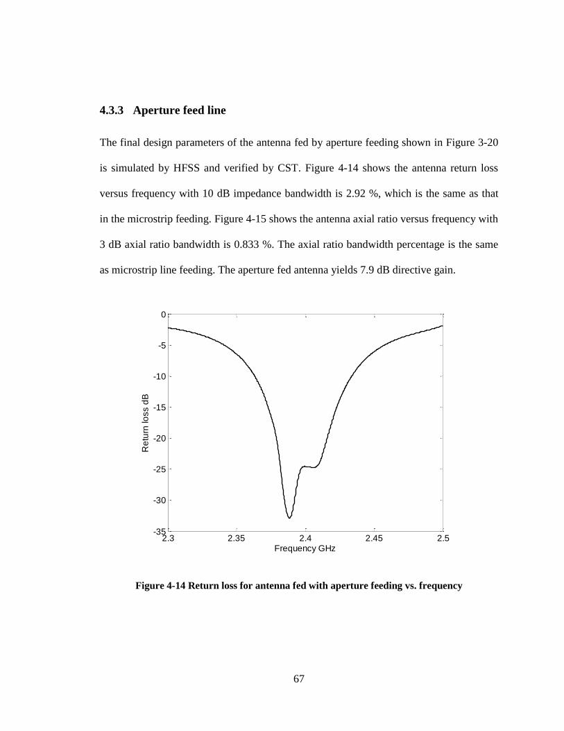
67

4.3.3 Aperture feed line

The final design parameters of the antenna fed by aperture feeding shown in Figure 3-20

is simulated by HFSS and verified by CST. Figure 4-14 shows the antenna return loss

versus frequency with 10 dB impedance bandwidth is 2.92 %, which is the same as that

in the microstrip feeding. Figure 4-15 shows the antenna axial ratio versus frequency with

3 dB axial ratio bandwidth is 0.833 %. The axial ratio bandwidth percentage is the same

as microstrip line feeding. The aperture fed antenna yields 7.9 dB directive gain.

Figure ‎4-14 Return loss for antenna fed with aperture feeding vs. frequency

2.3 2.35 2.4 2.45 2.5-35

-30

-25

-20

-15

-10

-5

0

Frequency GHz

Re

turn

lo

ss d

B

68

Figure ‎4-15Axial ratio for antenna fed with aperture feeding vs. frequency

Figure 4-16 and Figure 4-17 show the co and cross-polarization in the E-plane (φ = 0°,

180°) and H-plane (φ = 90°, 270°) respectively using HFSS. The figures show that the

antenna is right hand circularly polarized with half power beamwidth ≈ 72.5° in the E-

plane and ≈75° in the H-plane. The difference between the co and cross-polarization in

both the E and H-planes ≈ 29.9 dB, which is less than that with microstrip feeding but

more than that with proximity feeding.

2.35 2.4 2.450

0.5

1

1.5

2

2.5

3

3.5

4

4.5

5

Frequency GHz

Axia

l ra

tio

dB

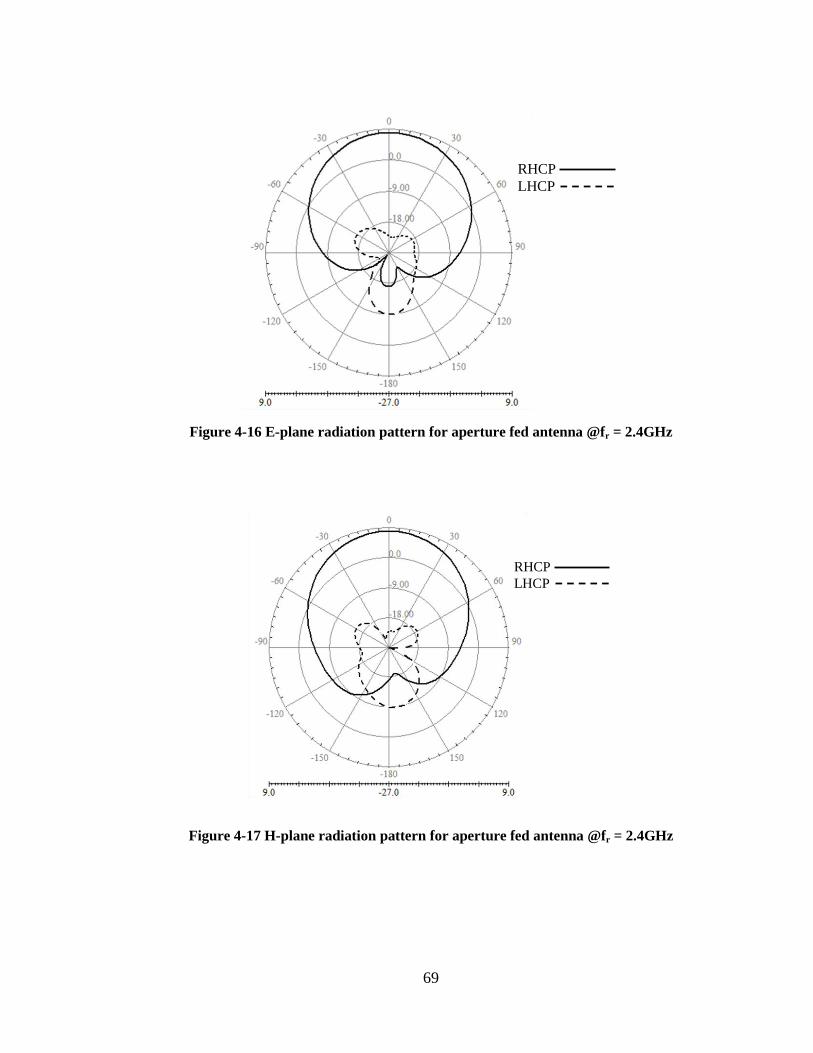
69

Figure ‎4-16 E-plane radiation pattern for aperture fed antenna @fr = 2.4GHz

Figure ‎4-17 H-plane radiation pattern for aperture fed antenna @fr = 2.4GHz

RHCP

LHCP

RHCP

LHCP

70

4.4 Comparison between the 3 antennas

Table 4-1 shows comparison between the 3 antennas in terms of dimensions and radiation

characteristics

Point of comparison Microstrip

feed

Proximity

feed

Aperture feed

rad mm 23.96 23.3 22.9

d 22.6 21.35 21.6

Wf 4.88 4.62 4.36

Impedance bandwidth % 2.92 5.36 2.92

Axial ratio bandwidth % 0.833 1.45 0.833

Directive antenna gain dB 8.11 8 7.9

Design frequency GHz 2.4 2.4 2.4

Difference between co and cross-

polarization in E-plane dB

31.08 28.14 29.9

Difference between co and cross-

polarization in H-plane dB

31.08 28.14 29.9

Half power beamwidth in the E-

plane °

70 70 72.5

Half power beamwidth in the H-

plane

73 77.5 75

Table ‎4-1 Comparision between the 3 types of single feeding

4.5 Summary

Comparing the results of the actual return loss measured results and the simulation results

obtained using HFSS and CST. The measured results and the HFSS results achieve the

minimum return loss at the same frequency 2.415 GHz; however the measured results

and the CST results follow the same curve shape.

71

Feeding microstrip antenna with three different types of single feeding techniques affects

the antenna output and dimensions.

The microstrip fed antenna is the easiest to model and fabricate. It possesses the largest

antenna size compared with the other two antennas to resonate at 2.4 GHz. It has the 10

dB impedance bandwidth as the aperture fed antenna. It has the highest isolation between

the co and cross – polarization.

The proximity fed antenna has the largest 10 dB impedance bandwidth and 3 dB axial

ratio bandwidth among the two other antennas. The aperture fed antenna is the smallest in

size than the other two antennas. It is the hardest to model. It has the same 10 dB return

loss and 3 dB axial ratio bandwidth as the microstrip fed antenna. After all simulations

and parametric studies were performed, results verifications was done using CST

Table 4-1 shows a comparison between the three single feeding schemes

72

Chapter 5

Conclusion and future work

5.1 Conclusion

The work presented focused on designing a circularly polarized microstrip antenna

operating at 2.4 GHz. The thesis presented a new design based on truncating 2 opposite

edges from a circular patch antenna. Three design versions were presented. The first

design used microstrip line feeding, the second used proximity feeding and the third used

aperture feeding.

Although the microstrip feeding needs a quarter wave length transformers between the

antenna and the 50 line feed and it is not easy to match, it is the easiest antenna to

model and simulate. Only two parametric studies were performed for choosing the

optimum values for the antenna radius and the distance between the antenna center and

the perturbation segment. The antenna radius is inversely proportional to the frequency.

73

The return loss value increases with increasing the distance between the antenna radius

and the perturbation segment. Increasing the distance between the patch canter and the

perturbation segments get 2 modes closer to each other near the design frequency. The

depth of the perturbation segment controls the circular polarization production. It is the

largest antenna in size among the other 2 antennas

The proximity feeding doesn’t need any matching as it doesn’t contact the 50 feed line.

But it is more complex than the microstrip feeding in modeling and optimization. It

requires three parametric studies to determine the optimum values for the antenna radius,

perturbation distance and the length of the feed line. The antenna radius is inversely

proportional to the frequency. The same effect as microstrip feeding when increasing the

perturbation segment distance on getting two modes closer. The length of the feed line

affects the antenna return loss and almost has no effect on the axial ratio.

The aperture feeding doesn’t need any matching too, but it is the most difficult antenna of

the three. It requires four parametric studies for determining the optimum values for

antenna radius, the perturbation distance from the patch center, the feed line length and

the ground slot radius. Like the other two antennas the antenna radius is inversely

proportional to the frequency and with increasing the perturbation distance two modes get

closer near the design frequency. The slot dimension affect the circular polarization

production, it acts like another perturbation segment. The feed line length affects the

antenna return loss value, but doesn’t have much effect on the axial ratio value. It is the

smallest antenna in size among the other 2 antennas

74

Feeding the same antenna with three different types of single feeding to radiate at the

same frequency; showed some difference in the antenna size and the radiation

characteristics.

Results show that microstrip fed antenna yields 8.11 dB directive gain, axial ratio and

impedance bandwidth 0.83 % and 2.92 % respectively. The proximity fed antenna yields

8 dB directive gain, axial ratio and impedance bandwidth 1.45 % and 5.36 % respectively.

The aperture fed antenna yields 7.92 dB directive gain, axial ratio and impedance

bandwidth 0.83 % and 2.92 % respectively.

5.2 Future work

One of the main advantages of a single fed microstrip antenna is that it can be used in the

production of antenna array. This work can be extended by investigating the design of an

antenna array that uses the antenna presented as its unit element. The future array

structure should investigate the use of the 3 feeding techniques presented as well. It

should also investigate the arrangement of the array elements.

Another interesting issue is to drive an empirical formula relating the depth of the

truncation with the antenna radius and the design frequency.

75

References

[1] John L. Volakis, Antenna Engineering Handbook 4th

edition, McGraw-Hill, 2007.

[2] Thomas A. Milligan, Modern Antenna Design 2nd

edition, John Wiley & Son Inc,

2005.

[3] D. M. Pozar, Microwave and RF Design of Wireless Systems, John Wiley & Son,

Inc, 2001.

[4] Wen-Shyang Chen, Chun-Kun Wu, Kin-Lu Wong, “Novel Compact Circularly

Polarized Square Microstrip Antenna,” IEEE Transactions on Antennas and

Propagation, Vol. 49, Issue. 3, 2001, pp. 340 – 342 .

[5] P. Serka, D. Bhatnagar, V.K. Saxena, J.S.Saini, “Single Feed Circularly Polarized

Edge Truncated Elliptical Microstrip Antenna,” in proceedings of the International

Conference on Emerging Trends in Electronic and Photonic Devices and Systems

ELECTRO, 2009, pp. 353-356.

[6] Wen-Shyang Chen, Chun-Kun Wu, Kin-Lu Wong, "Compact Circularly-Polarised

Circular Microstrip Antenna with Cross-Slot and Peripheral Cuts," IEEE

Electronics Letters, vol. 34, issue 11, 1998 , pp.1040-1041.

[7] Nasimuddin, Y. Yong, Z.N. Chen, A. Alphones, “Circularly Polarized F-Shaped

Slot Microstrip Antenna with Wide Beamwidth,” in proceedings of the European

Microwave Conference, EuMC , 2009 , pp. 1531–1534.

[8] G. A. Deschamps, “Microstrip Microwave Antennas,” in proceedings of the 3rd

USAF symposium on antennas, 1953.

76

[9] H. Gutton, G. Baissinot, “Flat Aerial for Ultra High Frequencies,” French Patent,

No.70313, 1955.

[10] David M.Pozar “Microstrip Antennas” IEEE proceedings, vol. 80, No.1, 1992, pp.

79-91.

[11] R. Garg, P. Bhartia, I. Bahl , A. Ittipiboon, Microstrip Antenna Design Handbook,

Arteck House, 2001.

[12] C. A. Balanis, Antenna Theory Analysis and Design 3rd

edition, John Wiley &

Sons, Inc., 2005.

[13] Y. T. Lo, S. W. Lee, Antenna Handbook, Van Nostrand Reinhold, 1993.

[14] A. Y. Simba, M. Yamamoto, T. Nojima, K. Itoh, “Circularly Polarised Proximity-

Fed Microstrip Antenna with Polarisation Switching Ability,” IET Microwaves

Antennas & Propagation, Vol.1, Issue. 3, 2007, pp. 658 – 665.

[15] Yen-Liang Kuo, Kin-Lu Wong, “A Circularly Polarized Microstrip Antenna with

a Photonic Band Gap Ground Plane,” in proceedings of Microwave Conference,

AMPC, Asia-Pacific , vol. 2, 2001 , pp. 647-650.

[16] David M. Pozar, Microwave Engineering 2nd

edition, John Wiley & Son, Inc.1998

[17] William H. Hayt, Jr. John A. Buck, Engineering Electromagnetic 6th edition,

McGraw-Hill, 2001.

[18] Samuel Silver, Microwave Antenna Theory and Design, McGraw-Hill 1949.

[19] IEEE Standard Test Procedures for Antennas, IEEE Std. 149-1979, Institute of

Electrical and Electronics Engineers, New York, 1979, sec. 11.

[20] Ron Schmitt, Electromagnetic Explained, Elsevier Science, 2002.

[21] Herbert P. Neff Jr., Introductory Electromagnetic, John Wiley & Son, Inc.1991.

[22] M. Rahmani, A. Tavakoli, H. R. Amindavar, A. M. Reza, P. Dehkhoda, “Chalipa,

a novel wideband circularly polarized microstrip fractal antenna” in proceedings of

the 3rd European Conference on Antennas and Propagation, EuCAP, 2009 ,pp.

2389 – 2392.

[23] K. Tamakuma, H. Iwasaki, “A Small Size Circularly Polarized Annular Microstrip

Antenna” in proceedings of the International Symposium IEEE Antennas and

Propagation Society, vol. 2, 2003, pp. 716 – 719.

[24] J. R. James, P s Hall, Handbook of Microstrip Antenna, vol.1, Peter Peregrinus Ltd.

1989.

77

[25] Y. Suzuki, N. Miyano, T. Chiba, “Circularly Polarised Radiation from Singly Fed

Equilateral-Triangular Microstrip Antenna,” IEE Proceedings on Microwaves,

Antennas and Propagation, vol. 134 , Issue. 2.

[26] Tso-Wei Li, Cheng-Liang Lai; Jwo-Shiun Sun, "Study of Dual-Band Circularly

Polarized Microstrip Antenna," proceedings of the European Conference on

Wireless Technology, 2005, pp. 79 – 80.

[27] J.-S. Row, C.-Y. Ai “Compact Design of Single-Feed Circularly Polarised

Microstrip Antenna” IEEE Electronics Letters, vol.40, issue: 18, 2004, pp. 1093-

1094.

[28] M. Haneishi; T. Nambara; S. Yoshida; “Study on Ellipticity Properties of Single-

Feed-Type Circularly Polarised Microstrip Antennas,” Electronics Letters, vol. 18,

Issue. 5, 1982, pp. 191 – 193.

[29] C. B. Ravipati, L. Shafai, "A wide Bandwidth Circularly Polarized Microstrip

Antenna Using a Single Feed," in proceeding of the IEEE Antennas and

Propagation Society International Symposium, vol.1, 1999, pp. 244-247.

[30] T. Sudha, T. S. Vedavathy, N. Bhat, “Wideband Single-Fed Circularly Polarised

Patch Antenna,” IEE Electronic Letters, vol. 40, issue. 11, 2004, pp. 648 – 649.

[31] P. N. Rao, N. Sarma, “Compact Single Feed Circularly Polarized Fractal Boundary

Microstrip Antenna” Electromagnetic Interference & Compatibility, 2008, pp. 347-

350

[32] P. N. Rao, N. Sarma, “Minkowski Fractal Boundary Single Feed Circularly

Polarized Microstrip Antenna,” Microwave and Optical Technology letters, Vol.

50, Issue. 11, 2008, pp. 2820–2824.

[33] P. N. Rao, N. Sarma, “A T-Type Fractal Boundary Single-Feed Circularly

Polarized Microstrip Antenna” International Journal of RF and Microwave

Computer-Aided Engineering,vol.19, issue: 2, 2009, pp. 285–291.

[34] P. N. Rao, N. Sarma, “Probe Compensated Single Feed Circularly Polarized

Fractal-Shaped Microstrip Antennas” International journal of RF and Microwave

Computer-Aided Engineering, vol.19, issue: 6, 2009, pp. 647–656.

[35] P. N. Rao; N. Sarma, “Fractal Boundary Circularly Polarised Single Feed

Microstrip Antenna,” IEEE Electronics Letters, vol. 44, issue:12, 2008, pp 713-

714.

[36] Nasimuddin, Z.N.Chen, Xianming Qing, “Single Fed Circularly Polarized

Microstrip Antenna with C-Slot,” in proceedings of the Microwave Conference,

2008, pp. 1-4.

78

[37] Nasimuddin, Xianming Qing, Zhi Ning Chen, “Microstrip Antenna with S-Shaped

Slot for Dual-Band Circularly Polarized Operation” in proceedings of the European

Microwave Conference, EuMC, 2009, pp. 381-384.

[38] H. Iwasaki; “A Circularly Polarized Small-Size Microstrip Antenna with a Cross

Slot”, IEEE Transactions on Antennas and Propagation, vol. 44, issue. 10, 1996,

pp. 1399-1401.

[39] Yufeng Wang, Jianjie Feng, Jingbo Cui, Xiaolong Yang, “A Dual-Band Circularly

Polarized Stacked Microstrip Antenna with Single-Fed for GPS Applications,” in

proceedings of the 8th International Symposium on Antennas Propagation and EM

Theory, ISAPE, 2008, pp. 108 – 110.

[40] M. Ali, R. Dougal, G.Yang, H-S. Hwang, “Wideband Circularly Polarized

Microstrip Patch Antenna for 5-6 GHz Wireless LAN Applications,” in proceeding

of the IEEE Antennas and Propagation Society International Symposium, Vol. 2,

2003, pp. 34-37.

[41] Wen-Shyang Chen, Kin-Lu Wong, Chun-Kun Wu, “Inset-Microstripline-Fed

Circularly Polarized Microstrip Antennas” in proceedings of the IEEE Antennas

and Propagation Society International Symposium, vol. 48, issue 8, 1999, pp 1253-

1254.

[42] Ansoft, High Frequency Structure Simulator (HFSS )program.

[43] Rogers Corporation, Computer aided program MWI-2010

[44] CST, Microwave Studio Computer Simulation Technology.

79

Publications

[1] Marwa Shakeeb, Hany Hammad, Abdelrasik Sebak, “Comprehensive study of

single feeding techniques on circularly polarized circular microstrip antenna

radiation pattern,” in the proceeding of the IEEE Middle East Conference for

Antenna and Propagation (MECAP), 2010.