Embed Size (px)
Citation preview

Physics and Physical Oceanography Technical Report 2000-1
Circulation Through
the Narrows of St. John’s Harbour: Summer and Fall 1999
Brad deYoung, Douglas J. Schillinger, Len Zedel and
Jack Foley
© 2000 Department of Physics and Physical Oeanography
Memorial University of Newfoundland St. John’s, Newfoundland
A1B 3X7
ii
Abstract
Current, temperature, fluorescence and surface elevation are presented from St. John’s
harbour for 24 July to 27 August and 12 October to 9 November 1999. Two Acoustic
Doppler Current Profiler’s (ADCPs) were deployed in July/August and one in
October/November to measure the current velocities at the mouth of the harbour.
Analysis of the current data shows that the flow over the sill is quite complex. The mean
flow had a three-layer structure in July/August and a two-layer flow in
October/November. The mean flow at the surface is out of the harbour during both
periods. Transports computed from the current data were compared with results obtained
using surface elevation observations from the harbour. There was reasonable agreement
at tidal periods but very poor agreement at subtidal periods. Currents in the centre of the
channel were not representative of the entire channel at subtidal frequencies. The
amplitudes and phases of the five primary tidal constitutents show relatively little vertical
structure except for the semi-diurnal band in July/August for which there is clear
evidence of a baroclinic tide. An energetic band at about 0.5 cycles per day, coherent
with the wind, was observed in July/August, but not in October/November.

iii
Acknowledgements
We thank the St. John’s Harbour Authority, in particular the Harbour Master, for
permission to fool around in the middle of the channel - a rather busy spot. The Harbour
Master also provided us with a detailed survey chart of the Narrows. We thank the divers
from the Ocean Sciences Centre for their support and for working in a difficult area. We
acknowledge the financial support of Environment Canada and the St. John’s ACAP.

iv
Table of Contents
Abstract ............................................................................................................................... ii
Acknowledgements............................................................................................................ iii
Table of Contents............................................................................................................... iv
List of Tables ...................................................................................................................... v
List of Figures ................................................................................................................... vii
Introduction......................................................................................................................... 1
Station Information ............................................................................................................. 2
Data Analysis ...................................................................................................................... 2
Interpretation....................................................................................................................... 4
Summary ........................................................................................................................... 10
References:........................................................................................................................ 11
July Data Set ..................................................................................................................... 12
October Data Set ............................................................................................................... 17

v
List of Tables Table 1: Mooring Locations................................................................................................ 2
Table 2: Summary Statistics of ADCP currents from mid-channel station (see Figure 1)..................................................................................................................................... 12
Table 3: Tidal height analysis of surface elevation data measured at the head of the harbour. ...................................................................................................................... 12
Table 4: Main Constituents of the Tidal Currents, July: Depth 1 m................................. 13
Table 5: Main Constituents of the Tidal Currents, July: Depth 2 m................................. 13
Table 6: Main Constituents of the Tidal Currents, July: Depth 3 m................................. 13
Table 7: Main Constituents of the Tidal Currents, July: Depth 4 m................................. 13
Table 8: Main Constituents of the Tidal Currents, July: Depth 5 m................................. 14
Table 9: Main Constituents of the Tidal Currents, July: Depth 6 m................................. 14
Table 10: Main Constituents of the Tidal Currents, July: Depth 7 m............................... 14
Table 11: Main Constituents of the Tidal Currents, July: Depth 8 m............................... 14
Table 12: Main Constituents of the Tidal Currents, July: Depth 9 m............................... 15
Table 13: Main Constituents of the Tidal Currents, July: Depth 10 m............................. 15
Table 14: Main Constituents of the Tidal Currents, July: Depth 11 m............................. 15
Table 15: Main Constituents of the Tidal Currents, July: Depth 12 m............................. 15
Table 16: Main Constituents of the Tidal Currents, July: Depth 13 m............................. 16
Table 17: Main Constituents of the Tidal Currents, July: Depth 14 m............................. 16
Table 18: Summary statistics of currents from the mid-channel station. ......................... 17
Table 19: Tidal height analysis from surface elevations measured at the head of the harbour. ...................................................................................................................... 17
Table 20: Main Constituents of the Tidal Currents, October: Depth 3 m......................... 18

vi
Table 21: Main Constituents of the Tidal Currents, October: Depth 4 m......................... 18
Table 22: Main Constituents of the Tidal Currents, October: Depth 5 m......................... 18
Table 23: Main Constituents of the Tidal Currents, October: Depth 6 m......................... 18
Table 24: Main Constituents of the Tidal Currents, October: Depth 7 m......................... 19
Table 25: Main Constituents of the Tidal Currents, October: Depth 8 m......................... 19
Table 26: Main Constituents of the Tidal Currents, October: Depth 9 m......................... 19
Table 27: Main Constituents of the Tidal Currents, October: Depth 10 m....................... 19
Table 28: Main Constituents of the Tidal Currents, October: Depth 11 m....................... 20
Table 29: Main Constituents of the Tidal Currents, October: Depth 12 m....................... 20
Table 30: Main Constituents of the Tidal Currents, October: Depth 13 m....................... 20
Table 31: Main Constituents of the Tidal Currents, October: Depth 14 m....................... 20
Table 32: Main Constituents of the Tidal Currents, October: Depth 15 m....................... 21

vii
List of Figures
Figure 1: Location of upward looking ADCP (green star), and cross-channel ADCP (July only, purple star). …………………………………………………22
Figure 2: Three dimensional topographic view of St. John’s Harbour. ………………...22 Figure 3: Time series of surface elevation, current velocity along the channel
axis (15 degrees from earth axes) at 3, 9 and 14 metres measured at the mid-channel station, and the magnitude of the wind stress……………………..23
Figure 4: Time series of surface elevation, current velocity across the channel
axis (15 degrees from earth axes) at 3, 9 and 14 metres measured at the mid-channel station, and the magnitude of the wind stress……………………..24
Figure 5: The power spectral density in deciBels for the along channel component
of velocity…………………………………………………………………….…25 Figure 6: The coherence squared between the East-West component of wind stress
and the along channel current velocity…………………………………………..26 Figure 7: The major and minor axes of the M2 tidal constituent. ………………………27 Figure 8: The major and minor axes of the K1 tidal constituent. ………………….…….28 Figure 9: The mean along (solid blue line) and cross (dashed red line) channel
velocity profiles………………………………………………………………….29 Figure 10: Surface elevation, velocity at 3, 9 and 14 m and wind stress with respect
to Earth axes……………………………………………………………………...30 Figure 11: The surface elevation at hourly intervals, and subtidal intervals. In both
plots the elevation is measured in cm, and the time line is measured in year day…………………………………………………………………………..31
Figure 12: The surface elevation, along channel velocity, temperature and wind stress
(with respect to Earth Axes), filtered to remove energy for periods above 1.6 days…………………….…………………………………………………….32
Figure 13: The surface elevation, backscatter intensity, temperature and wind stress,
filtered to remove energy for periods above 1.6 days...………………………….33 Figure 14: The surface elevation, along channel current velocity, backscatter intensity,
temperature and wind stress for Year day 218 to 222..………………………… 34

viii
Figure 15: The surface elevation, transport inferred from the measured elevation, and
the transport calculated from the along channel velocity component in are plotted against year day….………………………………………………………35
Figure 16: The velocity, in cm s-1, measured by the into-harbour beam of the cross-
channel ADCP…..……………………………………………………………….36 Figure 17: The velocity, in cm s-1, measured by the out-of-harbour beam of the cross-
channel ADCP….………………………………………………………………. 37 Figure 18: The power spectral density in deciBels for the velocity measured by the
into-harbour beam of the cross channel ADCP…..………………….…………..38 Figure 19: The power spectral density in deciBels for the velocity measured by the
out-of-harbour beam of the cross channel ADCP…..……………………………39 Figure 20: Temperature, salinity, and density profiles for 5 days in October taken
at the mid-channel station… …………………………………………………….40 Figure 21: Time series of surface elevation, current velocity along the channel
axis (15 degrees from earth axes) at 3, 9 and 14 metres measured at the mid- channel station, and the magnitude of the wind stress….……………………….41
Figure 22: Time series of surface elevation, current velocity across the channel axis
(15 degrees from earth axes) at 3, 9 and 14 metres measured at the mid- channel station, and the magnitude of the wind stress….……………………… 42
Figure 23: The power spectral density in deciBels for the along channel component
of velocity… ……………………………………………………………………43 Figure 24: The coherence squared between the East-West component of wind stress
and the along channel current velocity. ..………………………………………44 Figure 25: The major and minor axes of the M2 tidal constituent…………………...…45 Figure 26: The major and minor axes of the K1 tidal constituent...…………………….46 Figure 27: The mean along (solid blue line) and cross (dashed red line) channel
velocity profiles……………………………………………………………….. 47 Figure 28: Surface elevation, velocity at 3, 9 and 14 m and wind stress with respect
to Earth axes. …………………………………………………………………48 Figure 29: The surface elevation at hourly intervals, and subtidal intervals..………….49

ix
Figure 30: The surface elevation, along channel velocity, temperature and wind stress (with respect to Earth Axes), filtered to remove energy for periods above 1.6 days……………………………………………………………………50
Figure 31: The surface elevation, backscatter intensity, temperature and wind
stress, filtered to remove energy for periods above 1.6 days...…………………. 51 Figure 32: The surface elevation, along channel current velocity, backscatter
intensity, temperature and wind stress for Year day 286 to 290...……………….52 Figure 33: The surface elevation, transport inferred from the measured elevation, and the
transport calculated from the in-harbour velocity component in are plotted against year day..………………………………………………………………………... 53
Figure 34: The surface elevation, along channel current velocity, backscatter
intensity, temperature and wind stress showing the high velocity event of year day 297..…………………………………………………………………… 54
Introduction
The city of St. John’s is located on the Northeast coast of the Avalon Peninsula on
the Island of Newfoundland, Canada. The harbour mouth opens to the east, has a large
sill and a narrow entry to a shallow protected bay that has a somewhat deeper basin in
the northeastern half of the harbour. The mean depth of the harbour is about 12-15 m,
the sill depth is 13 m and the width of the harbour mouth is approximately 180 m. The
deepest point of the harbour is about 33m. The channel leading to the sill, the Narrows, is
approximately 800 m long and the harbour itself is about 1200m long. The harbour has a
surface area of approximately 1.2 million square metres. The cross sectional area of the
harbour mouth at the location of central channel mooring (depth 17m) is approximately
1600 square metres (Figure 1).
During the summer and fall of 1999 an upward-looking Acoustic Doppler Current
Profiler (ADCP) was deployed in the centre of the harbour mouth at a depth of 17 m (see
Figures 1 and 2). Our primary goal was to determine the circulation over the sill and the
implications of the transport for the exchange of water into and out of the harbour. In
July/August, an additional cross-channel-looking ADCP was deployed to one side of the
harbour mouth at a depth of 5 m. Temperature sensors were located on the ADCP’s and a
fluorometer was deployed on the ADCP in the centre of the channel. Surface height data
from the head of the harbour was obtained from the MEDS website (www.meds-
sdmm.dfo-mpo.gc.ca/meds/Home_e.htm).
Mooring data is tabulated with statistics on the maximum, minimum, mean and
variance in each velocity component in Tables 2 and 18 for July and October
respectively. The velocity data are presented graphically: time series at selected depths,
power spectral density of the hourly time series, profile plots, tidal ellipse plots and low-
pass filtered sub-tidal plots. We also calculated the transport from the current data and
the observed surface elevation. Tidal analysis was conducted on both the velocity and
height data. The results are presented graphically, with summary statistics in tabular
format.

2
Station Information
Near the sill, the channel entering St. John’s Harbour is very narrow, measuring
less than 200m across and we expected that a single mooring deployed in the centre of
the channel at this location would provide reasonable measurements of the average along-
channel velocity. Given the channel geometry, we believed that most of the flow would
be directed along the axis of the channel. The additional ADCP deployed in August in
side-looking mode was located on the southern side of the channel, pointed across the
channel towards Chain Rock (see Figure 1). Both instruments provided useful data,
which are presented and discussed in this report, although the side-looking ADCP only
measured sensible currents on the far side of the channel.
Table 1: Mooring Locations
Deployment Latitude Longitude Bin Width (m)
Depth (m) Start Stop
Sampling Interval (minutes)
Upward-Looking 47 33.97 52 41.29 1 17 24-Jul-99 27-Aug-99 20
Cross-Channel 47 33.97 54 34.98 8 17 24-Jul-99 27-Aug-99 20
Upward-Looking 47 33.97 54 41.29 1 18 12-Oct-99 09-Nov-99 20
Data Analysis
Data collected during the deployment and recovery of the instruments were first
clipped from all the records. Isolated incidents of bad data points were eliminated using a
simple linear interpolation scheme. For both the July and October data, all the bad data
points were limited to periods near the times of deployment and recovery.

3
We determined the along-channel and cross-channel axes through a covariance
analysis to locate the angle that minimized the variance along one component of a set of
perpendicular axes. For both July and October, the result of this analysis was depth
dependent, with October showing less variation in the angle with depth. The average
orientation was 15o clockwise rotation in July/August and 22o clockwise rotation in
October (see Figure 1). To minimise the cross channel velocity variation, the angles
corresponding to each individual deployment were chosen, however, the difference in
angle between deployments was only 7o.
The surface was located by examining the backscatter intensity contours and
identifying the depth bin with the most intense backscatter signal. Additional depth bins
were discarded on the basis of shear in the velocity profile. For the upward looking
ADCP, this resulted in the additional exclusion of two depth bins below the bin that
recorded the maximum backscatter intensity in July and three depth bins in October. For
the cross-channel velocity contour plots, the backscatter intensity contours are included
because of the large intensity backscatter signal from intermediate bins. In the vertical,
the depth resolution was roughly 1 m; for the side-looking instrument the horizontal
resolution was roughly 8 m.
For tidal analysis, we applied the harmonic analysis routines of Foreman (1977),
which require that the time series be in hourly intervals. To this end, data for the tidal
analysis were first filtered using a third order low-pass Butterworth filter with a pass band
of 3 hours and a stop band of period 2 hours in order to remove high frequency
fluctuations in the data. The data were then subsampled at 1-hour intervals as required by
the tidal analysis software. For consistency with the results from Foreman’s analysis, the
entire data set was smoothed with the low-pass filter and subsampled at hourly intervals.
Although the length of the record allows for the determination of several
additional constituents, only five primary constituents are included: MSf, O1, K1, M2
and S2. The calculation was performed using a Rayleigh scaling factor of 2.0 for the July
data set and 3.0 for the October data set. Both the axes of the representative tidal-
ellipses and the corresponding Greenwich phase describe the main constituents of the
tidal currents. The inclination of the ellipse indicates the angle the semi-major axis
makes with the positive x-axis (15 and 22 o clockwise rotation for July and October

4
respectively). A positive value for the length of the semi-major axis indicates that the
current rotates counter clockwise around the tidal ellipse, while a negative value indicates
a clockwise rotation.
In addition to the summary information provided from the harmonic analysis, the
time series were filtered using a least squared method to remove tidal signals at the MSf,
O1, K1, M2 and S2 frequencies. The residual of this filter was then low-pass filtered with
a third order Butterworth filter set to energy at periods shorter than 1.6 days.
Interpretation
Time series plots (Figures 3 and 4) show that the along-channel velocity is much
greater than that across the channel, by a factor of 5-10 in speed. Covariance analysis was
used to rotate the axis to maximize the along-channel velocity. This rotation was 15o
clockwise for the July/August deployment and 22o for the October/November
deployment. The degree of rotation did show some depth dependence but the difference
between the surface and the bottom was less than 5o. The mean difference between the
two deployments may arise from differing oceanographic conditions or perhaps from the
small difference in the location of the two deployments (which may differ by as much as
5-10 metres across the channel and perhaps 10-20 metres along the channel).
The power spectrum for currents in July/August shows clear peaks at 0.5 cycles
per day (cpd), 1 cpd and 2 cpd (Figure 5). The M2 tide shows remarkably little vertical
structure in amplitude, even though it is baroclinic, while there does appear to be a
minimum in the K1 tide at mid-depths. The peak at 0.5 cpd is interesting as it is obviously
not tidally forced. Energy at this period shows substantial depth dependence with a
minimum centered at about 7 m. We explored coherence (Figure 6) between the current
and different representations of the wind stress (amplitude, x and y components of stress,
x and y components of stress in the rotated channel coordinates). The only significant
coherence squared is at 0.5 cpd.
Tidal analysis was carried out on the u and v components in the rotated co-
ordinate system. Although both components of velocity are included, clearly most of the
5
energy is in the along-channel component. The semi-diurnal components dominate, in
particular the M2 that has an amplitude of 34.7 cm (Table 3). The tables of the
constituent analysis for the currents (Tables 4-17) and the plots of the tidal ellipses
(Figures 7 and 8 for July/August) show that there is some depth dependence to the tidal
current, although there is little depth dependence in the amplitude: 2.39 cm s-1 for M2 at
the surface and 1.95 cm s-1 at the bottom, in July. There is some evidence of baroclinicity
in the M2 tide but not in the K1 tide. For July, the K1 tide shows a phase difference from 1
to 14 m that is less than 12 degrees; for the M2 tide the phase difference is roughly 163
degrees, indicating that the baroclinic response is primarily in mode 1. All the diurnal and
semi-diurnal constituents show similar structure. As might be expected, given the change
in stratification from July/August to October/November, with the increasing depth of the
surface mixed layer and the reduced stratification between the upper and lower layers,
there is no evidence of a baroclinic response in October/November. For this period, the
phase difference from 3 to 13 m is less than 1o for M2 and 16o for K1.
The mean currents (Figure 9) show that the mean cross-channel current is
approximately zero, as expected, but that there is significant depth dependence to the
mean along-channel currents There is a mean outward surface current of about 4 cm s-1
near the surface, driven by the freshwater inflow from the Waterford River and sewage
dumping. Surprisingly, the surface outflow is restricted to the top few metres of the water
column, not very deep. There is also outflow at depth, below 10m, with inflow between 3
and 10m. The variance about these mean values is quite large (Figure 9). Plots of the
spatial structure of the along-channel current (Figure 10) show that the spectral peak at
0.5 cpd is an inflow event covering most of the water column but is punctuated by
outflow events near the bottom. There is not much evidence of energy at two-day periods
(Figure 11) in the subtidal surface elevation. The outflow events which follow (or lead?)
the inflows, are bottom intensified. The relationship between the inflows and outflows is
unknown. The inflows begin near the bottom and spread to the surface as they develop.
These observations, with uni-directional flow in the channel over most of the water
column for day-long periods, raise questions about the cross-channel structure of the
flow. The strong mean inflow at mid-depths is determined by this 0.5 cpd activity. The
low-pass currents are also correlated with changes in water column particle concentration

6
as determined by the strength of the acoustic backscatter signal (Figure 13). Plots of the
raw data for short periods (Figure 14) show that the low-frequency signal does in fact
dominate and that the tidal signal is barely apparent. There is also a strong relationship
between the backscatter intensity and the orientation and strength of the flow. For
example, the bottom outflows around day 219 lead to substantial increases in the
backscatter intensity, which rises off the bottom, matching the character of the bottom
inflow event. This event shows that not all increases in backscatter intensity are
associated with outflow events.
We also used the data to determine the transport over the sill, at subtidal and tidal
periods. The transport from the current was determined by multiplying the current at each
depth by the cross sectional channel area at that depth. We compared the results of this
calculation with the observed net flux as determined from the rate of change of elevation
in the harbour times the surface area of the harbour. At tidal periods we get generally
reasonable agreement, within about 10% at the M2 period. For the K1 tide in
July/August, the current data overpredicts the transport by about a factor of 1.5. The
subtidal transport from the current data has a range of about –200 to + 200 m3s-1. The
surface elevation data give a range in transport of –100 to + 100 m3s-1. The current
transport calculation significantly overestimates the flux. While there may be some
difficulties for the subtidal calculation, these differences are very large. That we get the
M2 correct confirms that the ADCP is measuring sensible currents through the channel. It
is reasonable that we should get the transport for the strongest and clearest tidal
constituent correct. That we overpredict the K1 tide is probably because this tidal
constituent is weaker and the tidal analysis of the current meter data is pulling in some of
the energy at other periods. It is clear from the raw data (Figure 3) that there is a lot of
non-tidal energy in the currents, much more than in the elevation data.
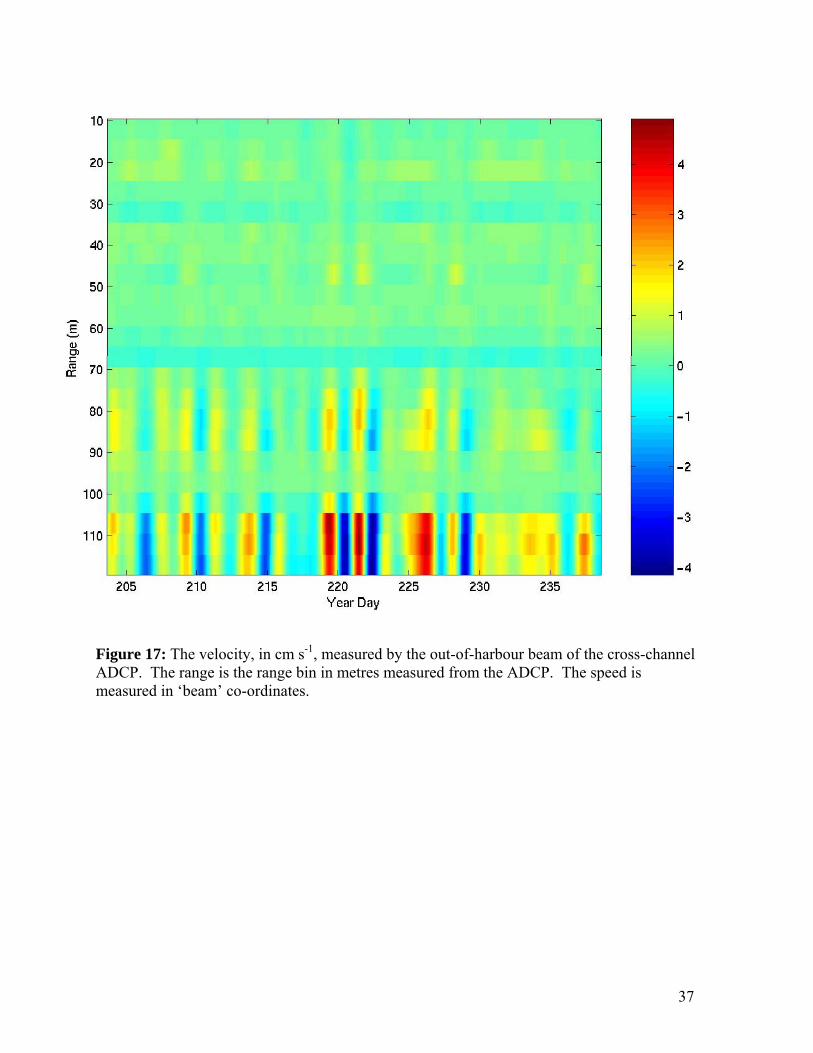
The cross-channel data are somewhat disappointing. We looked at the velocity
from the two separate beams. For these data, we have not used averaged beam velocities,
but instead use the speed from each beam separately. For about the first 50 metres, there
is only a weak velocity signal in either beam (Figures 16 and 17). Beyond 50 m,
however, the inward facing beam (pointing somewhat into the harbour) does show
similar spectral peaks to the upward looking instrument, confirming that it is detecting
7
real currents (Figures 18 and 19). The other beam, which was pointing just outside of
chain rock, does not show such a clear pattern and between 90 and 100 m shows a decline
in spectral energy at almost all frequencies. We do not have a complete explanation for
these observations but believe that the outward looking beam is being influenced by
sidelobe interference between 90 and 100 m, causing a reduction in signal intensity.
Separate plots of the velocity (Figures 16 and 17) reveal that in the far-field, beyond 80m,
the two instruments show opposing velocities, perhaps indicating flow around the
topographic features (Chain Rock) on the northern side of the channel.
There is very little thermal stratification in October, although there is a strong
salinity gradient from the surface down to 5 m (Figure 20). Although the raw time series
again show a predominance of along-channel flow (Figures 21 and 22) the
October/November data reveal many differences from the observations in July/August.
Note that the peak in the cross channel flow on day 297 is real and will be discussed later.
As expected there is still energy at the tidal periods, the diurnal and the semi-diurnal, and
there is also energy at the inertial period, roughly 1.5 cpd, as there is in July/August. The
tidal peaks here are more dominant than in July/August. The wind-forced response at 0.5
cpd is again present in October/November although it is somewhat weaker than was
observed in the July/August data (Figure 23). Coherence analysis again shows the
relation between the wind and the currents at 0.5 cpd (Figure 24). One might expect the
October/November wind-forced response to be stronger, given that wind forcing is more
intense, however, the internal response may be stratification dependent. We suspect that
the wind forcing at the two-day period is a result of forcing outside the harbour in the
coastal waveguide in the Avalon Channel and that an internal Kelvin wave response is
generated that rises up and enters the harbour, at a roughly two-day period (de Young et
al. 1993, Davidson et al. 1999). Further modelling, and perhaps an expanded observation
program, will be necessary to test this hypothesis.
The plots for the tidal ellipses show (Figures 25 and 26) the relative absence of
vertical structure in the tidal signal discussed earlier. The mean currents in
October/November (Figure 27) look much more like the expected two-layer circulation
of an estuary with an outflow of about 4 cm s-1 at 3 m and inflow below 5 m depth with a
peak inflow of over 6 cm s-1 at about 10m depth. Even a cursory glance at these plots

8
shows that there is more inflow than outflow, raising questions about the cross-channel
structure of the along-channel flow. Stick plots of the velocity once again show that
although the along-channel flow dominates, there is some vertical structure to the flow
and bottom topographic steering is not uniform with depth (Figure 28). Surface elevation
plots indicate a relation between strong wind events (e.g. just before day 290) and rising
surface elevation (Figure 29).
The subtidal, along-channel currents show that the surface outflow is not steady
but occurs in pulses of a few days duration that are linked to strong inflow events that
extend from 8 m depth to the bottom (Figure 30). The surface outflow is restricted to the
upper 5m with the strongest currents above 3m depth. Strong southwesterly winds do
appear to be correlated with these exchange events, in particular, the strongest exchange
around days 287-288 is correlated with the strongest wind event of the record
corresponding to strong southerly winds that turn to southwesterly as they develop.
The backscatter plot (Figure 31) shows that at times there is some correlation
between the inflow/outflow events and particle concentrations, but this is not consistent.
Thus the first strong event does have the largest particle concentration, but is restricted to
the surface waters. The other strong backscatter event is during the period from days 296-
300. The structure of this event is more uniform with depth. Once again the raw data
plots at hourly intervals (Figure 32) show that the low-frequency currents dominate.
There is little energy at tidal periods, and a clear relationship between the strong outflow
event around day 287.5 and the increase in the backscatter intensity near the surface, with
no obvious connection with the wind, which lags this event.
The October/November tidal transport calculations from the currents and
elevation agree to within 10% for both the M2 and K1 tides. It is apparent from the time
series that the October data (Figure 21) shows much stronger tidal transport, relative to
the subtidal, than do the July data (Figure 3). The subtidal transport calculations again
show poor agreement between the currents and elevation (Figure 33). Not only is there
poor agreement but the currents overpredict the amplitude by about a factor of three. The
lower panel in Figure 33 shows that the total transport as determined from our current
meter data is always into the harbour. This result is not physically sensible and indicates
that there is a strong gradient in the cross-channel structure of the flow. The transport as

9
determined from the observed surface elevation (Figure 33) shows that the maximum
transport is roughly 10 m3 s-1, a much more reasonable result and one that is expected
given that the mean freshwater inflow in this system is of order 1 m3 s-1.
What about the residence time for water in the Harbour? If we take the
mean depth as about 12-15 m then the total volume of the harbour is about 1.5 x 10⁷ m3 .
The maximum transport in July/August as calculated from the surface elevation is about
5 m3s-1, which would correspond to an exchange time of 34 days for all the harbour
water. If we take the maximum transport from the current calculations, then we get an
exchange time of less than 2-3 days. The surface elevation from October/November gives
a maximum transport of 10 m3s-1 giving an exchange time of about 17 days. The current
transport from October/November gives an exchange time of less than 2-3 days. The
surface elevation transport result probably provides an exchange time that is too long,
while the current determined transport provides an exchange time that is too short. Water
in the harbour is not completely mixed. Water in the northeastern half of the harbour
probably has a much shorter exchange time than water in the southwestern half. In
particular, surface water in the northeastern corner probably has the shortest residence
time of all the water in the harbour. The average exchange period for the harbour is 5-15
days, perhaps even shorter during periods of particularly strong forcing.
But what about the effect of tidal exchange? The strongest tides in the system are
the semidiurnal tides, the M2 and S2 , with amplitudes of roughly 2-4 cm s-1 . The semi-
diurnal tidal transport through the narrows is therefore about 50 m3s-1. During flood tide
this corresponds to an inflow of somewhat less than 10% of the total volume of the
harbour giving an exchange time of about 6-7 days. Combining the subtidal and tidal
exchange estimates suggests that the real exchange rate is probably closer to the five-day
period than it is to the fifteen-day period. This shorter exchange rate is consistent with the
observed high oxygen levels in the surface and the deeper water of the harbour.
The large cross-channel velocity that appears around day 297 and stands out in
Figure 22 is apparently real and is not an artifact. Close inspection of the data for this
period reveals that there is strong inflow and outflow, beginning just after 3:00 PM local
time on 25 October. The currents are so strong that the instrument is knocked off its
location and its orientation disrupted, as shown by large, abrupt changes in the internal

10
inclination sensors. The current during the period is strongly into and then out of the
channel, oscillating with a twenty minute period (Figure 34), or perhaps less since the
sampling period is twenty minutes. There is no response the elevation in the harbour, nor
is there anything obvious in either the wind time series or the temperature data. These
data show that the winds in St. John’s were in fact quite light. At the same time large
seiches, or harbour waves, were generated in Petty Harbour, Port Rexton and Little
Catalina (B. Whiffen, Environment Canada, personal communication). The seiche in
Petty Harbour was several metres in amplitude with a period of tens of minutes, running
over the dock, and persisting for several hours.
The event in St. John’s harbour did not generate a seiche in the basin but did have
some substantial effect on the circulation in the Narrows. Indeed, the backscatter time
series (Figure 34) shows that particle concentrations dramatically increased throughout
the water column, with the greatest intensity at the bottom. This event in the backscatter
took several hours to dissipate. These events could have been forced by some external
wave, perhaps a tsunami associated with a shelf-break slumping event or the passage of a
dissipating hurricane.
Summary
These data tell us a number of interesting things about the transport through the
Narrows into St. John’s harbour:
(1) Tidal circulation is not particularly dominant.
(2) The summer circulation is at least as strong as that observed in the late fall, perhaps
stronger.
(3) Even during the summer, the wind forced transport at a period of roughly 2 days
generates large transports and large velocities through the narrows.
(4) Surface elevation shows substantial subtidal variability but the response at 2 days
period is primarily baroclinic and not barotropic.
(5) We estimate the mean residence time of water in the Harbour to be roughly 5-10
days.

11
(6) Current shear across the channel is substantial, in particular at subtidal periods, and
the strong inflow that we observe in the centre of the channel must be balanced by
strong outflows along the sides of the channel.
We believe that the shape and position of the Narrows is important in determining
the currents that we report on as measured here at the western end of the Narrows
(Figure 1). Note that the Narrows is 2-3 times wider at its eastern end than it is to the
west where it attaches to the harbour. Water flowing in through this channel
accelerates as it enters the harbour, thereby leading to the strong jet that we see on
inflow events. The opposite will happen on outflow and it must be that the strong
outflow is concentrated along the sides of the channel away from the centre of the
channel. A mooring program with additional instruments across the channel is
required to close the transport over the sill of St. John’s Harbour.
References:
deYoung, B., Otterson, T. and R. Greatbatch. 1993. The local and non-local response of
Conception Bay to wind forcing. J. Phys. Ocean., 23, 2636-2649.
Davidson, F. , Greatbatch, R. and B. deYoung. 2000. Asymmetry in the response of a
stratified coastal embayment to wind forcing. J. Geophys. Res. (in press).
Foreman, M. Manual for Tidal Heights Analysis and Prediction, Pacific Marine Science
Report 78-6, Institute of Ocean Sciences, Patricia Bay, Victoria B.C., (1977)

12
July Data Set Table 2: Summary Statistics of ADCP currents from mid-channel station (see Figure 1).
Depth (m) Component Max (cm s-1) Min (cm s-1) Mean (cm s-1) Std (cm s-1) 1 v 11.76 0.01 -0.81 2.39 u 35.21 0.00 3.34 9.15 2 v 9.31 0.00 -0.69 1.87 u 32.94 0.00 1.53 9.01 3 v 6.87 0.01 -0.83 1.80 u 33.10 0.00 -1.11 8.50 4 v 8.13 0.00 -1.06 1.74 u 31.96 0.03 -3.11 7.65 5 v 7.80 0.01 -1.23 1.55 u 35.01 0.01 -4.48 7.04 6 v 7.13 0.01 -1.41 1.55 u 34.93 0.01 -5.06 6.86 7 v 8.10 0.00 -1.43 1.62 u 37.86 0.00 -5.02 7.01 8 v 8.11 0.00 -1.41 1.64 u 37.35 0.00 -4.27 7.58 9 v 7.84 0.00 -1.48 1.59 u 40.37 0.02 -2.82 8.56
10 v 6.97 0.00 -1.63 1.58 u 41.86 0.01 -1.03 9.58
11 v 6.86 0.02 -1.69 1.57 u 41.99 0.03 0.94 10.43
12 v 8.15 0.01 -1.96 1.75 u 41.55 0.02 2.74 11.02
13 v 8.81 0.01 -2.04 1.90 u 40.12 0.04 4.41 11.33
14 v 10.00 0.00 -1.76 1.96 u 37.54 0.02 5.69 11.55
Table 3: Tidal height analysis of surface elevation data measured at the head of the harbour.
Name Frequency Amplitude G. Phase Z0 0.00000000 83.30 0.00
MSf 0.00282193 1.09 10.9 O1 0.03873065 6.63 320.3 K1 0.04178075 9.57 130.5 M2 0.08051140 34.67 95.0 S2 0.08333334 12.41 269.9

13
The main tidal constituents of the July data set from the mid-channel station (Figure 1). Table 4: Main Constituents of the Tidal Currents, July: Depth 1 m. Name Frequency Major Axis
(cm s-1) Minor Axis
(cm s-1) Inclination G. Phase
Z0 0.00000000 3.30 0.00 166.2 180.0 MSf 0.00282193 0.50 -0.21 163.5 70.5 O1 0.03873065 0.38 0.33 59.2 351.3 K1 0.04178075 2.38 -0.06 1.4 144.3 M2 0.08051140 2.39 0.16 5.3 307.1 S2 0.08333334 2.00 0.05 176.9 186.1
Table 5: Main Constituents of the Tidal Currents, July: Depth 2 m. Name Frequency Major Axis
(cm s-1) Minor Axis
(cm s-1) Inclination G. Phase
Z0 0.00000000 1.58 0.00 154.2 180.0 MSf 0.00282193 1.16 -0.12 6.3 273.5 O1 0.03873065 0.32 -0.11 8.7 181.9 K1 0.04178075 2.40 -0.07 1.0 151.2 M2 0.08051140 2.58 0.02 3.0 341.4 S2 0.08333334 2.22 -0.17 176.2 203.3
Table 6: Main Constituents of the Tidal Currents, July: Depth 3 m. Name Frequency Major Axis
(cm s-1) Minor Axis
(cm s-1) Inclination G. Phase
Z0 0.00000000 1.50 0.00 33.1 180.0 MSf 0.00282193 1.39 -0.07 0.8 278.4 O1 0.03873065 0.54 0.03 176.5 19.6 K1 0.04178075 2.16 -0.09 10.7 153.4 M2 0.08051140 2.83 0.15 5.3 342.3 S2 0.08333334 2.19 -0.17 178.3 203.3
Table 7: Main Constituents of the Tidal Currents, July: Depth 4 m. Name Frequency Major Axis
(cm s-1) Minor Axis
(cm s-1) Inclination G. Phase
Z0 0.00000000 3.43 0.00 17.8 180.0 MSf 0.00282193 1.42 0.01 1.5 275.4 O1 0.03873065 0.52 0.12 165.4 21.6 K1 0.04178075 1.81 0.06 14.0 143.2 M2 0.08051140 2.92 0.06 9.5 342.2 S2 0.08333334 2.32 0.05 2.9 23.3

14
Table 8: Main Constituents of the Tidal Currents, July: Depth 5 m. Name Frequency Major Axis
(cm s-1) Minor Axis
(cm s-1) Inclination G. Phase
Z0 0.00000000 4.77 0.000 14.8 180.0 MSf 0.00282193 1.30 -0.04 2.4 262.9 O1 0.03873065 0.43 0.09 0.1 231.7 K1 0.04178075 1.41 0.02 16.7 137.5 M2 0.08051140 2.91 0.05 10.1 339.6 S2 0.08333334 2.30 0.03 9.3 19.1
Table 9: Main Constituents of the Tidal Currents, July: Depth 6 m. Name Frequency Major Axis
(cm s-1) Minor Axis (cm s-1)
Inclination G. Phase
Z0 0.00000000 5.34 0.00 15.1 180.0 MSf 0.00282193 1.18 0.03 2.4 255.3 O1 0.03873065 0.33 0.05 19.0 306.5 K1 0.04178075 0.96 -0.10 6.3 120.1 M2 0.08051140 2.90 0.07 11.3 334.4 S2 0.08333334 2.11 0.12 11.7 15.6
Table 10: Main Constituents of the Tidal Currents, July: Depth 7 m. Name Frequency Major Axis
(cm s-1) Minor Axis (cm s-1)
Inclination G. Phase
Z0 0.00000000 5.29 0.00 15.7 180.0 MSf 0.00282193 0.94 0.04 4.0 250.8 O1 0.03873065 0.64 -0.07 15.6 330.8 K1 0.04178075 0.40 -0.18 13.7 101.5 M2 0.08051140 2.90 0.09 10.5 332.7 S2 0.08333334 1.90 0.18 10.0 11.0
Table 11: Main Constituents of the Tidal Currents, July: Depth 8 m. Name Frequency Major Axis
(cm s-1) Minor Axis (cm s-1)
Inclination G. Phase
Z0 0.00000000 4.54 0.00 18.2 180.0 MSf 0.00282193 0.84 0.06 5.3 240.6 O1 0.03873065 0.51 -0.05 15.5 333.6 K1 0.04178075 0.34 -0.11 30.5 345.9 M2 0.08051140 2.80 0.08 7.9 331.2 S2 0.08333334 1.75 0.11 4.6 11.0

15
Table 12: Main Constituents of the Tidal Currents, July: Depth 9 m. Name Frequency Major Axis
(cm s-1) Minor Axis
(cm s-1) Inclination G. Phase
Z0 0.00000000 3.22 0.00 27.3 180.0 MSf 0.00282193 0.74 0.03 9.8 241.6 O1 0.03873065 0.32 -0.15 179.7 175.8 K1 0.04178075 0.74 -0.09 179.2 170.3 M2 0.08051140 2.76 0.08 7.0 331.2 S2 0.08333334 1.69 0.19 9.5 14.9
Table 13: Main Constituents of the Tidal Currents, July: Depth 10 m. Name Frequency Major Axis
(cm s-1) Minor Axis
(cm s-1) Inclination G. Phase
Z0 0.00000000 1.94 0.00 56.0 180.0 MSf 0.00282193 0.80 -0.09 13.6 248.3 O1 0.03873065 0.26 0.08 17.9 95.3 K1 0.04178075 0.97 -0.12 176.4 163.8 M2 0.08051140 2.76 0.09 3.1 330.1 S2 0.08333334 1.58 0.17 7.0 18.1
Table 14: Main Constituents of the Tidal Currents, July: Depth 11 m. Name Frequency Major Axis
(cm s-1) Minor Axis (cm s-1)
Inclination G. Phase
Z0 0.00000000 1.87 0.00 118.8 180.0 MSf 0.00282193 0.70 -0.20 11.9 246.7 O1 0.03873065 0.46 -0.02 8.8 106.9 K1 0.04178075 1.20 -0.01 172.8 165.3 M2 0.08051140 2.65 0.07 179.6 149.0 S2 0.08333334 1.45 0.17 2.3 18.1
Table 15: Main Constituents of the Tidal Currents, July: Depth 12 m. Name Frequency Major Axis
(cm s-1) Minor Axis
(cm s-1) Inclination G. Phase
Z0 0.00000000 3.36 0.00 144.6 180.0 MSf 0.00282193 0.61 -0.12 13.3 240.9 O1 0.03873065 0.53 -0.02 175.3 300.8 K1 0.04178075 1.25 -0.18 165.1 160.9 M2 0.08051140 2.42 0.07 0.3 328.3 S2 0.08333334 1.49 0.11 2.8 22.1
16
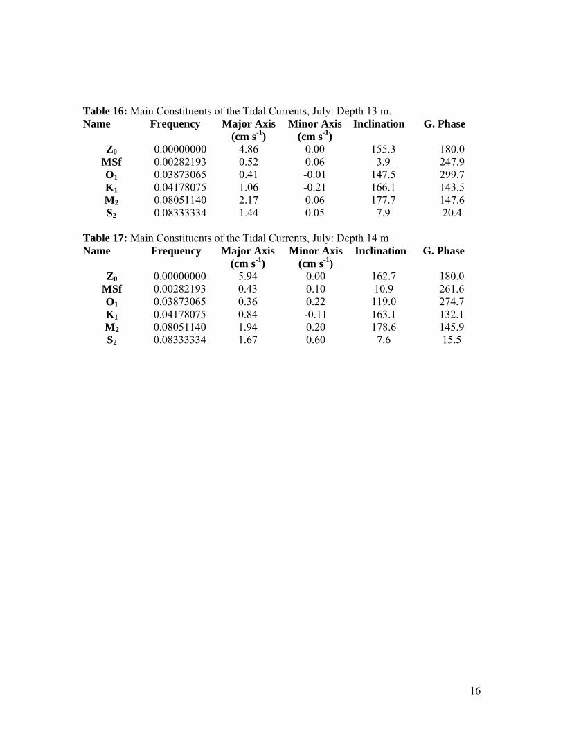
Table 16: Main Constituents of the Tidal Currents, July: Depth 13 m. Name Frequency Major Axis
(cm s-1) Minor Axis
(cm s-1) Inclination G. Phase
Z0 0.00000000 4.86 0.00 155.3 180.0 MSf 0.00282193 0.52 0.06 3.9 247.9 O1 0.03873065 0.41 -0.01 147.5 299.7 K1 0.04178075 1.06 -0.21 166.1 143.5 M2 0.08051140 2.17 0.06 177.7 147.6 S2 0.08333334 1.44 0.05 7.9 20.4
Table 17: Main Constituents of the Tidal Currents, July: Depth 14 m Name Frequency Major Axis
(cm s-1) Minor Axis
(cm s-1) Inclination G. Phase
Z0 0.00000000 5.94 0.00 162.7 180.0 MSf 0.00282193 0.43 0.10 10.9 261.6 O1 0.03873065 0.36 0.22 119.0 274.7 K1 0.04178075 0.84 -0.11 163.1 132.1 M2 0.08051140 1.94 0.20 178.6 145.9 S2 0.08333334 1.67 0.60 7.6 15.5
17
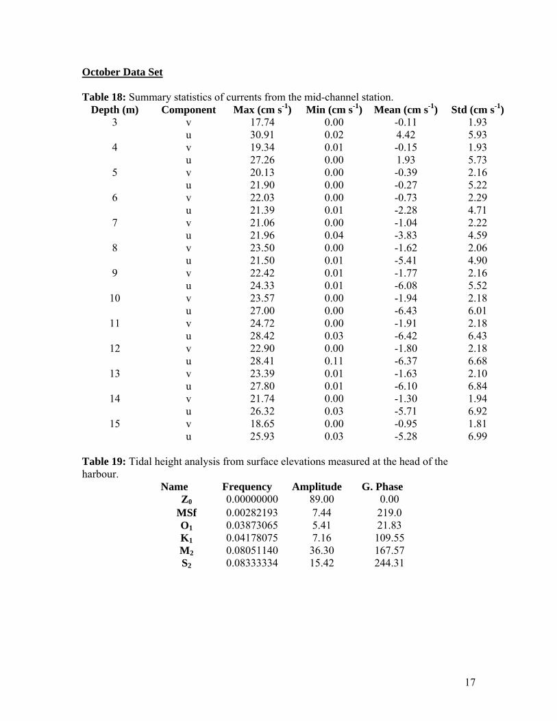
October Data Set Table 18: Summary statistics of currents from the mid-channel station.
Depth (m) Component Max (cm s-1) Min (cm s-1) Mean (cm s-1) Std (cm s-1) 3 v 17.74 0.00 -0.11 1.93 u 30.91 0.02 4.42 5.93 4 v 19.34 0.01 -0.15 1.93 u 27.26 0.00 1.93 5.73 5 v 20.13 0.00 -0.39 2.16 u 21.90 0.00 -0.27 5.22 6 v 22.03 0.00 -0.73 2.29 u 21.39 0.01 -2.28 4.71 7 v 21.06 0.00 -1.04 2.22 u 21.96 0.04 -3.83 4.59 8 v 23.50 0.00 -1.62 2.06 u 21.50 0.01 -5.41 4.90 9 v 22.42 0.01 -1.77 2.16 u 24.33 0.01 -6.08 5.52
10 v 23.57 0.00 -1.94 2.18 u 27.00 0.00 -6.43 6.01
11 v 24.72 0.00 -1.91 2.18 u 28.42 0.03 -6.42 6.43
12 v 22.90 0.00 -1.80 2.18 u 28.41 0.11 -6.37 6.68
13 v 23.39 0.01 -1.63 2.10 u 27.80 0.01 -6.10 6.84
14 v 21.74 0.00 -1.30 1.94 u 26.32 0.03 -5.71 6.92
15 v 18.65 0.00 -0.95 1.81 u 25.93 0.03 -5.28 6.99
Table 19: Tidal height analysis from surface elevations measured at the head of the harbour.
Name Frequency Amplitude G. Phase Z0 0.00000000 89.00 0.00
MSf 0.00282193 7.44 219.0 O1 0.03873065 5.41 21.83 K1 0.04178075 7.16 109.55 M2 0.08051140 36.30 167.57 S2 0.08333334 15.42 244.31

18
The main tidal constituents of the October data set from the mid-channel station (Figure1). Table 20: Main Constituents of the Tidal Currents, October: Depth 3 m. Name Frequency Major Axis
(cm s-1) Minor Axis
(cm s-1) Inclination G. Phase
Z0 0.00000000 4.31 0.00 178.0 180.0 MSf 0.00282193 1.66 0.21 175.1 357.6 O1 0.03873065 1.10 -0.09 173.4 202.2 K1 0.04178075 1.34 0.14 173.1 209.1 M2 0.08051140 3.74 -0.52 2.5 7.7 S2 0.08333334 1.76 0.13 1.1 39.0
Table 21: Main Constituents of the Tidal Currents, October: Depth 4 m. Name Frequency Major Axis
(cm s-1) Minor Axis
(cm s-1) Inclination G. Phase
Z0 0.00000000 1.83 0.00 173.9 180.0 MSf 0.00282193 1.38 0.34 5.8 208.8 O1 0.03873065 0.96 -0.03 179.6 200.4 K1 0.04178075 1.47 -0.07 179.9 220.5 M2 0.08051140 4.19 -0.36 4.5 12.6 S2 0.08333334 1.69 0.04 15.2 38.3
Table 22: Main Constituents of the Tidal Currents, October: Depth 5 m. Name Frequency Major Axis
(cm s-1) Minor Axis
(cm s-1) Inclination G. Phase
Z0 0.00000000 0.60 0.00 52.4 180.0 MSf 0.00282193 1.35 0.18 25.5 237.8 O1 0.03873065 0.72 0.07 9.0 27.2 K1 0.04178075 1.21 -0.20 4.2 44.8 M2 0.08051140 4.36 -0.16 8.1 14.9 S2 0.08333334 1.63 0.07 20.6 24.7
Table 23: Main Constituents of the Tidal Currents, October: Depth 6 m. Name Frequency Major Axis
(cm s-1) Minor Axis
(cm s-1) Inclination G. Phase
Z0 0.00000000 2.49 0.00 18.6 180.0 MSf 0.00282193 1.39 -0.11 35.6 265.5 O1 0.03873065 0.52 0.01 8.3 36.1 K1 0.04178075 0.83 -0.09 4.6 57.4 M2 0.08051140 4.48 -0.08 12.3 13.2 S2 0.08333334 1.65 0.08 20.8 14.1
19
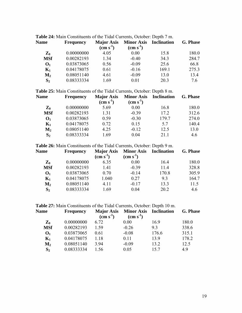
Table 24: Main Constituents of the Tidal Currents, October: Depth 7 m. Name Frequency Major Axis
(cm s-1) Minor Axis
(cm s-1) Inclination G. Phase
Z0 0.00000000 4.05 0.00 15.8 180.0 MSf 0.00282193 1.34 -0.40 34.3 284.7 O1 0.03873065 0.56 -0.09 25.6 66.8 K1 0.04178075 0.61 -0.16 169.1 275.3 M2 0.08051140 4.61 -0.09 13.0 13.4 S2 0.08333334 1.69 0.01 20.3 7.6
Table 25: Main Constituents of the Tidal Currents, October: Depth 8 m. Name Frequency Major Axis
(cm s-1) Minor Axis
(cm s-1) Inclination G. Phase
Z0 0.00000000 5.69 0.00 16.8 180.0 MSf 0.00282193 1.31 -0.39 17.2 312.6 O1 0.03873065 0.59 -0.30 179.7 274.0 K1 0.04178075 0.72 0.15 5.7 140.4 M2 0.08051140 4.25 -0.12 12.5 13.0 S2 0.08333334 1.69 0.04 21.1 4.6
Table 26: Main Constituents of the Tidal Currents, October: Depth 9 m. Name Frequency Major Axis
(cm s-1) Minor Axis (cm s-1)
Inclination G. Phase
Z0 0.00000000 6.35 0.00 16.4 180.0 MSf 0.00282193 1.41 -0.39 11.4 328.8 O1 0.03873065 0.70 -0.14 170.8 305.9 K1 0.04178075 1.040 0.27 9.3 164.7 M2 0.08051140 4.11 -0.17 13.3 11.5 S2 0.08333334 1.69 0.04 20.2 4.6
Table 27: Main Constituents of the Tidal Currents, October: Depth 10 m. Name Frequency Major Axis
(cm s-1) Minor Axis
(cm s-1) Inclination G. Phase
Z0 0.00000000 6.72 0.00 16.9 180.0 MSf 0.00282193 1.59 -0.26 9.3 338.6 O1 0.03873065 0.61 -0.08 176.6 315.1 K1 0.04178075 1.18 0.11 13.9 178.2 M2 0.08051140 3.94 -0.09 13.2 12.5 S2 0.08333334 1.56 0.05 15.7 4.9

20
Table 28: Main Constituents of the Tidal Currents, October: Depth 11 m. Name Frequency Major Axis
(cm s-1) Minor Axis
(cm s-1) Inclination G. Phase
Z0 0.00000000 6.67 0.00 16.9 180.0 MSf 0.00282193 1.67 -0.14 2.5 348.5 O1 0.03873065 0.66 0.00 0.6 140.5 K1 0.04178075 1.10 0.08 8.1 181.6 M2 0.08051140 3.95 -0.09 9.8 11.3 S2 0.08333334 1.43 -0.03 13.0 6.9
Table 29: Main Constituents of the Tidal Currents, October: Depth 12 m. Name Frequency Major Axis
(cm s-1) Minor Axis
(cm s-1) Inclination G. Phase
Z0 0.00000000 6.57 0.00 16.2 180.0 MSf 0.00282193 1.69 -0.16 179.9 179.6 O1 0.03873065 0.56 0.01 179.5 316.3 K1 0.04178075 0.98 0.06 17.4 180.4 M2 0.08051140 3.87 -0.24 8.1 9.8 S2 0.08333334 1.40 -0.08 8.9 9.9
Table 30: Main Constituents of the Tidal Currents, October: Depth 13 m Name Frequency Major Axis
(cm s-1) Minor Axis
(cm s-1) Inclination G. Phase
Z0 0.00000000 6.24 0.00 15.5 180.0 MSf 0.00282193 1.85 -0.13 175.8 185.4 O1 0.03873065 0.50 0.03 178.6 325.5 K1 0.04178075 0.87 0.03 21.2 193.6 M2 0.08051140 3.81 -0.22 5.5 8.3 S2 0.08333334 1.40 -0.06 2.3 9.4
Table 31: Main Constituents of the Tidal Currents, October: Depth 14 m Name Frequency Major Axis
(cm s-1) Minor Axis
(cm s-1) Inclination G. Phase
Z0 0.00000000 5.73 0.00 13.3 180.0 MSf 0.00282193 1.96 -0.11 177.5 193.1 O1 0.03873065 0.46 0.05 168.4 322.2 K1 0.04178075 0.75 0.03 15.8 192.1 M2 0.08051140 3.50 -0.23 4.0 7.4 S2 0.08333334 1.41 -0.13 179.4 192.7

21
Table 32: Main Constituents of the Tidal Currents, October: Depth 15 m Name Frequency Major Axis
(cm s-1) Minor Axis
(cm s-1) Inclination G. Phase
Z0 0.00000000 5.23 0.00 10.5 180.0 MSf 0.00282193 2.12 -0.14 0.7 21.3 O1 0.03873065 0.35 0.06 6.5 158.2 K1 0.04178075 0.72 -0.04 5.8 184.1 M2 0.08051140 3.29 -0.17 4.3 7.1 S2 0.08333334 1.24 -0.05 174.9 192.2

22
October
July
Figure 1: Location of upward looking ADCP (green star), and cross-channel ADCP (July only, purple star). Included are the orientation of the axes for the rotated frame of reference for both July and October. The mid-channel station for October was also at the green-star position.
Figure 2: Three dimensional topographic view of St. John’s Harbour. The shoreline and docks are overlaid in black. The depth scale is in metres, with the land set to zero and the harbour/sill bottom at negative depths.

23
Figure 3: Time series of surface elevation, current velocity along the channel axis (15 degrees from earth axes) at 3, 9 and 14 metres, and the magnitude of the wind stress. The surface elevation is measured in cm, and the current velocities are in cm s-1. The wind stress amplitude is measured in 0.1 N m-2.

24
Figure 4: Time series of surface elevation, current velocity across the channel axis (15 degrees from earth axes) at 3, 5 and 14 metres, and the magnitude of the wind stress. The surface elevation is measured in cm, and the current velocities are in cm s-1. The wind stress amplitude is measured in 0.1 N m-2.

25
Figure 5: The power spectral density in deciBels for the along channel component of velocity. The frequency is measured in cycles per day, and the depth is in metres. These spectra have 9 degrees of freedom.

26
Figure 6: The coherence squared between the East-West component of wind stress and the along channel current velocity. The coherence squared has 9 degrees of freedom.

27
Figure 7: The major and minor axes of the M2 tidal constituent. The axes represent velocities measured in cm s-1. For the three dimensional plot of the tidal ellipses, the red line represents the inclination of each tidal ellipse at depth, with respect to the rotated axes. Here E-W is the along-channel axis.

28
Figure 8: The major and minor axes of the K1 tidal constituent. The axes represent velocities measured in cm s –1. For the three dimensional plot of the tidal ellipses, the red line represents the inclination of each tidal ellipse at depth, with respect to the rotated axes. Here E-W is the along-channel axis.

29
Figure 9: The mean along (solid blue line) and cross (dashed red line) channel velocity profiles. The velocities are in cm s-1. The standard deviation of the velocity components for each depth are plotted as error bars. These velocities are computed in ‘channel’ co-ordinates (see text).

30
Figure 10: Surface elevation, velocity at 3, 9 and 14 m and wind stress with respect to Earth axes. The horizontal axis doubles as the year day, and the East-West axis, while the vertical axis represents the North-South axis, and shows the scale of the individual physical property. Included here are the surface elevation in cm, the current velocities in cm s-1, and the wind stress in N m-2.

31
Figure 11: The surface elevation at hourly intervals, and subtidal intervals. In both plots the elevation is measured in cm, and the time line is measured in year day.

32
Figure 12: The surface elevation, along channel velocity, temperature and wind stress (with respect to Earth Axes), filtered to remove energy for periods above 1.6 days. The time scale for each plot is in year day, while the individual physical properties are measured in cm, cm s-1, º C, and N m-2.

33
Figure 13: The surface elevation, backscatter intensity, temperature and wind stress, filtered to remove energy for periods above 1.6 days. The time line is in year day, while the individual physical properties are measured in cm, dB, º C, and N m-2.

34
Figure 14: The surface elevation, along channel current velocity, backscatter intensity, temperature and wind stress for Year day 218 to 222. The physical properties are measured in cm, cm s-1, dB, º C, and N m-2.

35
Figure 15: The surface elevation, transport inferred from the measured elevation, and the transport calculated from the along channel velocity component are plotted against year day. The transport is in m3 s-1, while the surface elevation is in cm.

36
Figure 16: The velocity, in cm s-1, measured by the into-harbour beam of the cross-channel ADCP. The range is the range bin in metres measured from the ADCP. The speed is measured in ‘beam’ co-ordinates.
37
Figure 17: The velocity, in cm s-1, measured by the out-of-harbour beam of the cross-channel ADCP. The range is the range bin in metres measured from the ADCP. The speed is measured in ‘beam’ co-ordinates.

38
Figure 18: The power spectral density in deciBels for the velocity measured by the into-harbour beam of the cross channel ADCP. The frequency is measured in cycles per day, and the depth is in metres. These spectra have 9 degrees of freedom.

39
Figure 19: The power spectral density in deciBels for the velocity measured by the out-of-harbour beam of the cross channel ADCP. The frequency is measured in cycles per day, and the depth is in metres. These spectra have 9 degrees of freedom.

40
Figure 20: Temperature, salinity, and density profiles for 5 days in October 1999 taken at the mid-channel station.

41
Figure 21: Time series of surface elevation, current velocity along the channel axis (22 degrees from earth axes) at 3, 9 and 14 metres measured at the mid-channel station, and the magnitude of the wind stress. The surface elevation is measured in cm, and the current velocities are in cm s-1. The wind stress amplitude is measured in 0.1 N m-2.

42
Figure 22: Time series of surface elevation, current velocity across the channel axis (22 degrees from earth axes) at 3, 9 and 14 metres measured at the mid-channel station, and the magnitude of the wind stress. The surface elevation is measured in cm, and the current velocities are in cm s-1. The wind stress amplitude is measured in 0.1 N m-2.

43
Figure 23: The power spectral density in deciBels for the along channel component of velocity. The frequency is measured in cycles per day, and the depth is in metres. These spectra have 7 degrees of freedom.

44
Figure 24: The coherence squared between the East-West component of wind stress and the along channel current velocity. The coherence squared has 7 degrees of freedom.

45
Figure 25: The major and minor axes of the M2 tidal constituent. The axes represent velocities measured in cm s-1. For the three dimensional plot of the tidal ellipses, the red line represents the inclination of each tidal ellipse at depth, with respect to the rotated axes. Here E-W is the along-channel axis.

46
Figure 26: The major and minor axes of the K1 tidal constituent. The axes represent velocities measured in cm s –1. For the three dimensional plot of the tidal ellipses, the red line represents the inclination of each tidal ellipse at depth, with respect to the rotated axes. Here E-W is the along-channel axis.

47
Figure 27: The mean along (solid blue line) and cross (dashed red line) channel velocity profiles. The velocities are in cm s-1. The standard deviation of the velocity components for each depth are plotted as error bars. These velocities are computed in ‘channel’ co-ordinates (see text).

48
Figure 28: Surface elevation, velocity at 3, 9 and 14 m and wind stress with respect to Earth axes. The horizontal axis doubles as the year day, and the East-West axis, while the vertical axis represents the North-South axis, and shows the scale of the individual physical property. Included here are the surface elevation in cm, the current velocities in cm s-1, and the wind stress in N m-2.
49
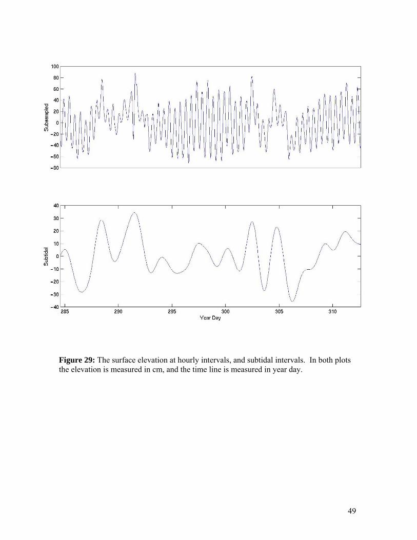
Figure 29: The surface elevation at hourly intervals, and subtidal intervals. In both plots the elevation is measured in cm, and the time line is measured in year day.

50
Figure 30: The surface elevation, along channel velocity, florescence, temperature and wind stress (with respect to Earth Axes), filtered to remove energy for periods above 1.6 days. The time scale for each plot is in year day, while the individual physical properties are measured in cm, cm s-1, μ g l-1, º C, and N m-2.

51
Figure 31: The surface elevation, backscatter intensity, florescence, temperature and wind stress (with respect to Earth Axes), filtered to remove energy for periods above 1.6 days. The time scale for each plot is in year day, while the individual physical properties are measured in cm, cm s-1, μ g l-1, º C, and N m-2.

52
Figure 32: The surface elevation, along channel current velocity, backscatter intensity, temperature and wind stress for Year day 286 to 290. The physical properties are measured in cm, cm s-1, dB, º C, and N m-2.

53
Figure 33: The surface elevation, transport inferred from the measured elevation, and the transport calculated from the along channel velocity component are plotted against year day. The transport is in m3 s-1, while the surface elevation is in cm.

54
Figure 34: The surface elevation, along channel current velocity, backscatter intensity, florescence, temperature and wind stress (with respect to Earth Axes), filtered to remove energy for periods above 1.6 days. The time scale for each plot is in year day, while the individual physical properties are measured in cm, cm s-1, μ g l-1, º C, and N m-2.