CISE301_Topic4 1

CISE301: Numerical Methods

Topic 4: Least Squares Curve

FittingLectures 18-19:

KFUPM

Read Chapter 17 of the textbook

CISE301_Topic4 2

Lecture 18Introduction to Least

Squares

CISE301_Topic4 3

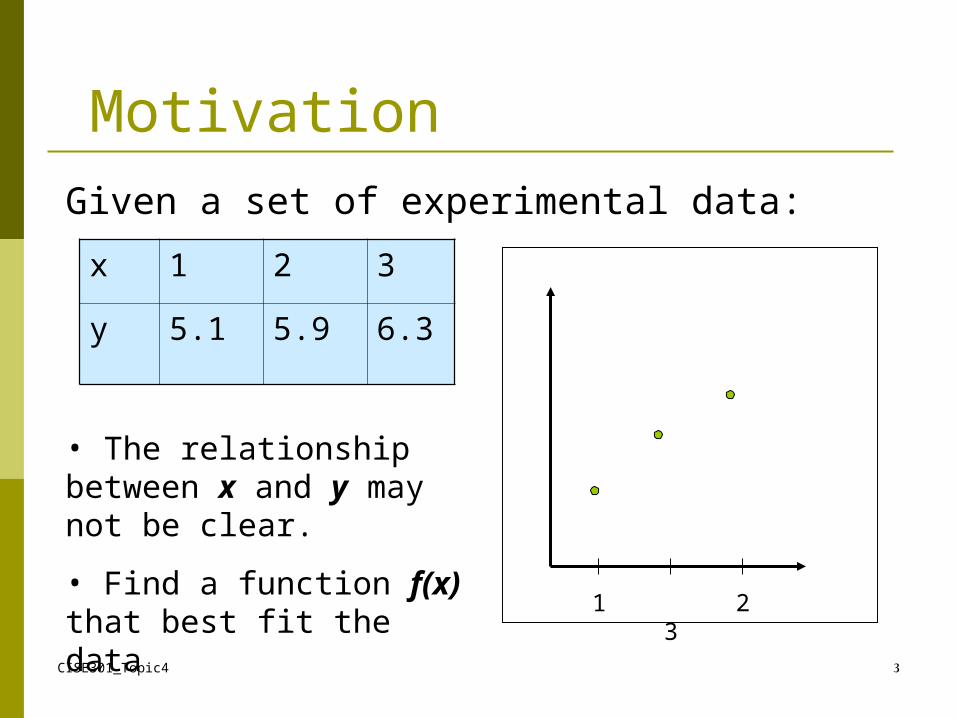
MotivationGiven a set of experimental data:

x 1 2 3

y 5.1 5.9 6.3

• The relationship between x and y may not be clear.

• Find a function f(x) that best fit the data

1 2 3

CISE301_Topic4 4

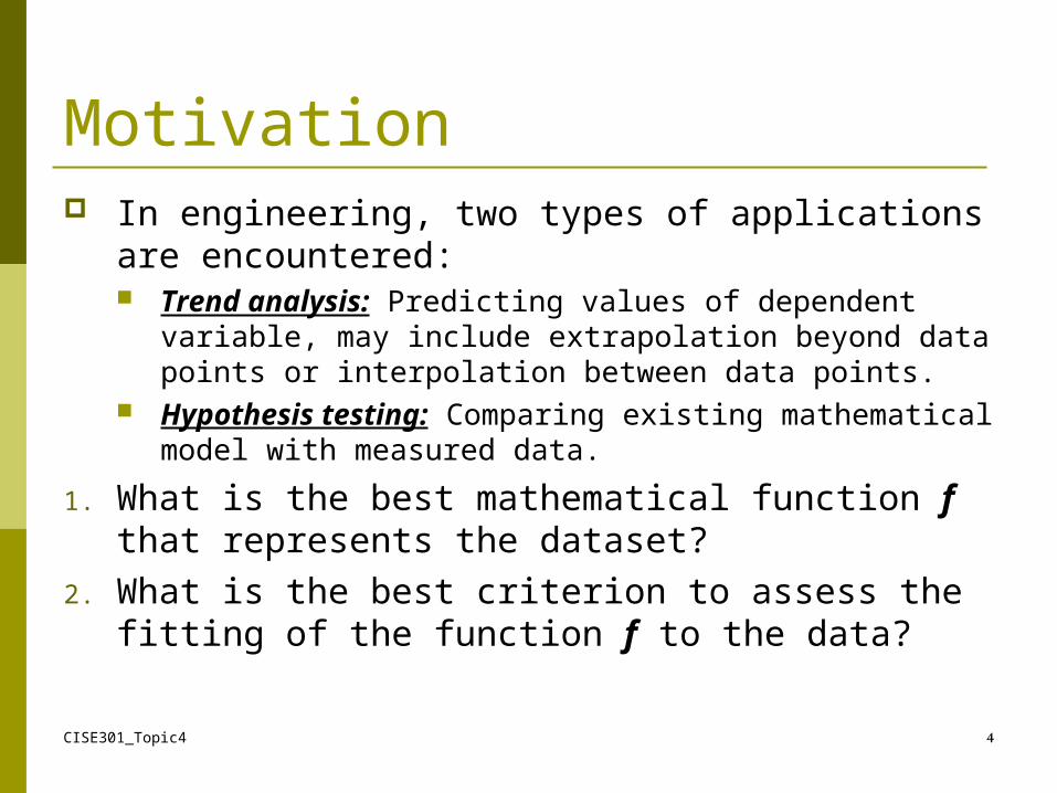
Motivation In engineering, two types of applications are

encountered: Trend analysis: Predicting values of dependent

variable, may include extrapolation beyond data points or interpolation between data points.

Hypothesis testing: Comparing existing mathematical model with measured data.

1. What is the best mathematical function f that represents the dataset?

2. What is the best criterion to assess the fitting of the function f to the data?

CISE301_Topic4 5

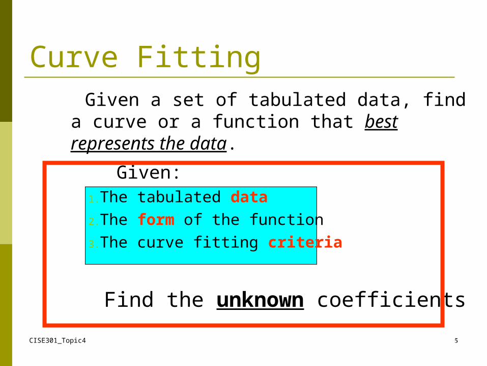
Curve Fitting Given a set of tabulated data, find a curve

or a function that best represents the data.

Given:1.The tabulated data2.The form of the function3.The curve fitting criteria

Find the unknown coefficients

CISE301_Topic4 6

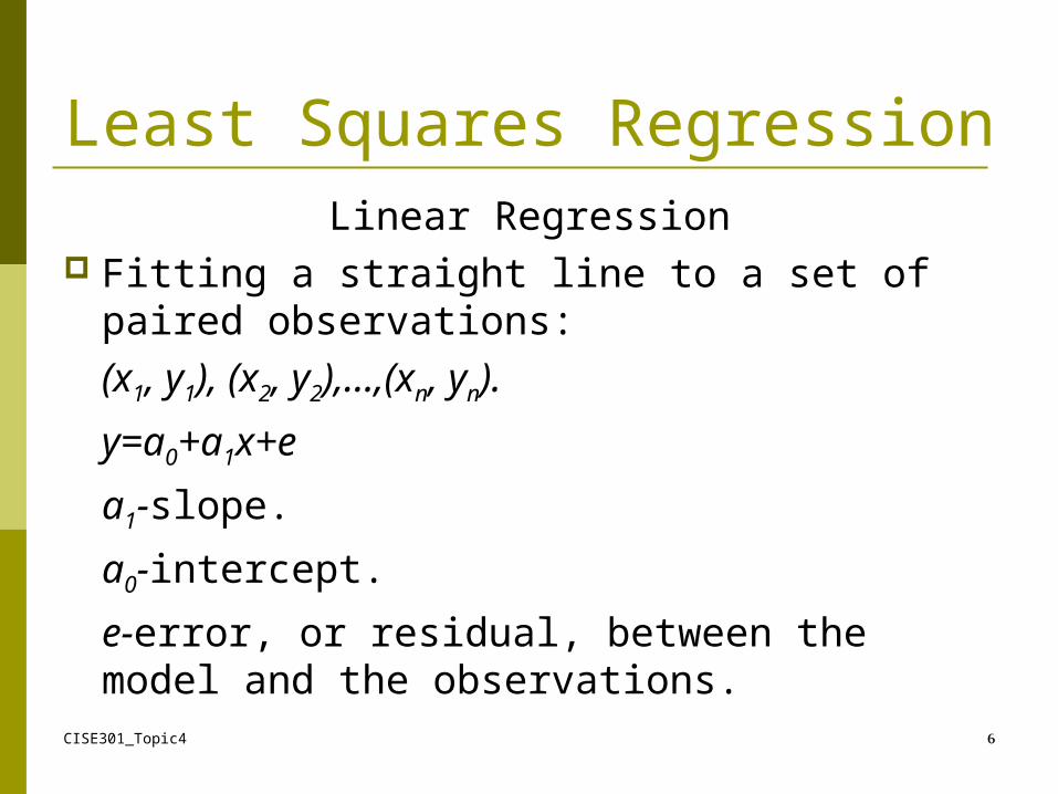
Least Squares RegressionLinear Regression

Fitting a straight line to a set of paired observations:(x1, y1), (x2, y2),…,(xn, yn).

y=a0+a1x+e

a1-slope.

a0-intercept.

e-error, or residual, between the model and the observations.

CISE301_Topic4 7

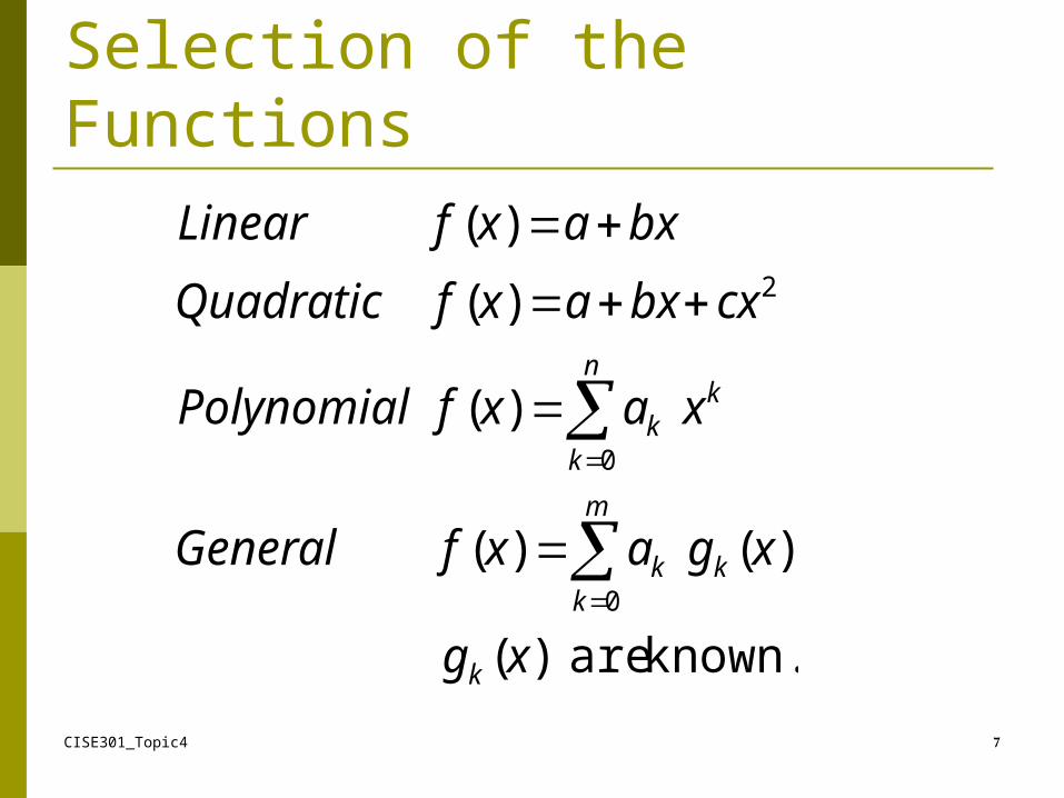
Selection of the Functions

known. are)(

)()(

)(

)(

)(

0

0

2

xg

xgaxfGeneral

xaxfPolynomial

cxbxaxfQuadratic

bxaxfLinear

k

m

kkk

n

k

kk

CISE301_Topic4 8

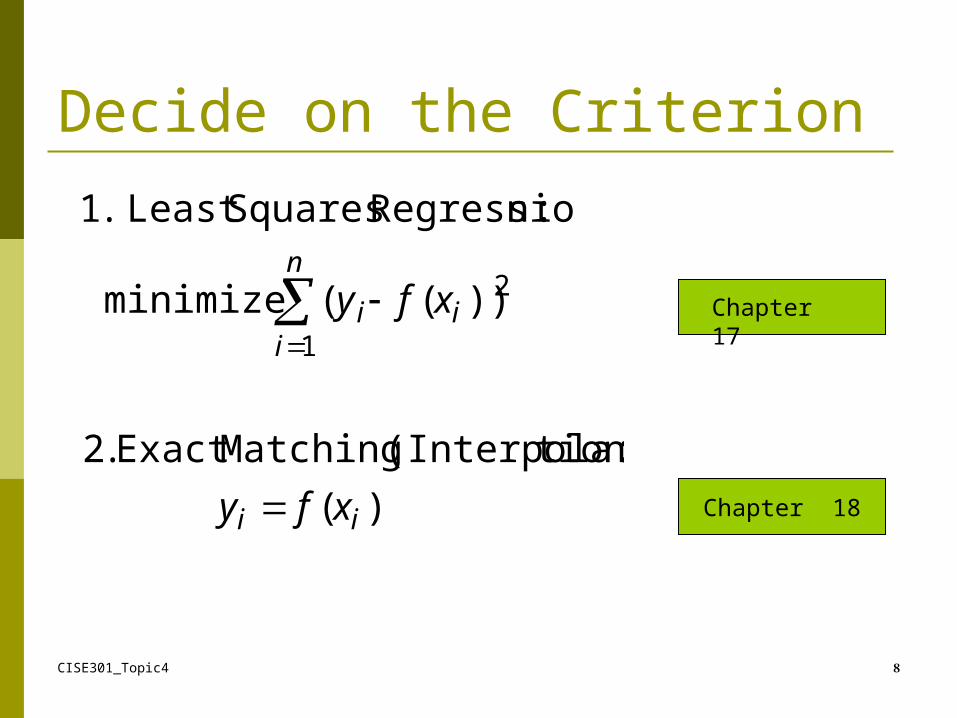
Decide on the Criterion

)(

:tion)(Interpola MatchingExact .2

))(( minimize

:n RegressioSquaresLeast .1

1

2

ii

n

iii

xfy

xfy

Chapter 17

Chapter 18

CISE301_Topic4 9

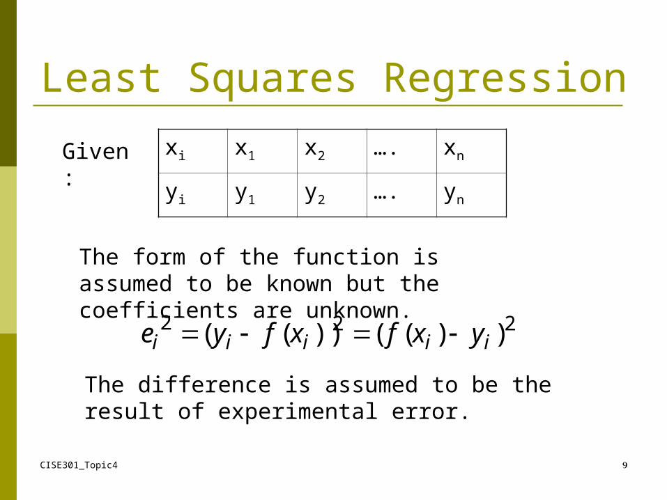
Least Squares Regression

xi x1 x2 …. xn

yi y1 y2 …. yn

Given:

The form of the function is assumed to be known but the coefficients are unknown.

222 ))(())(( iiiii yxfxfye

The difference is assumed to be the result of experimental error.

CISE301_Topic4 10

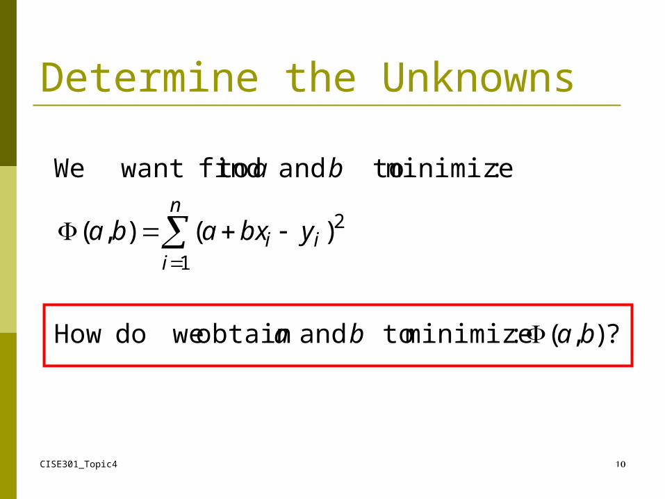
Determine the Unknowns

?),( :minimize to and obtain wedoHow

)(),(

:minimize to and find want toWe

1

2

baba

ybxaba

ban

iii

CISE301_Topic4 11

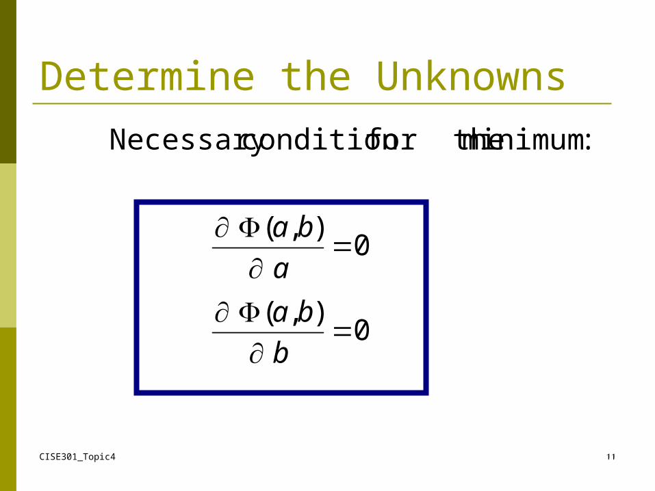
Determine the Unknowns

0),(

0),(

:minimum for the condition Necessary

b

ba

a

ba

CISE301_Topic4 12

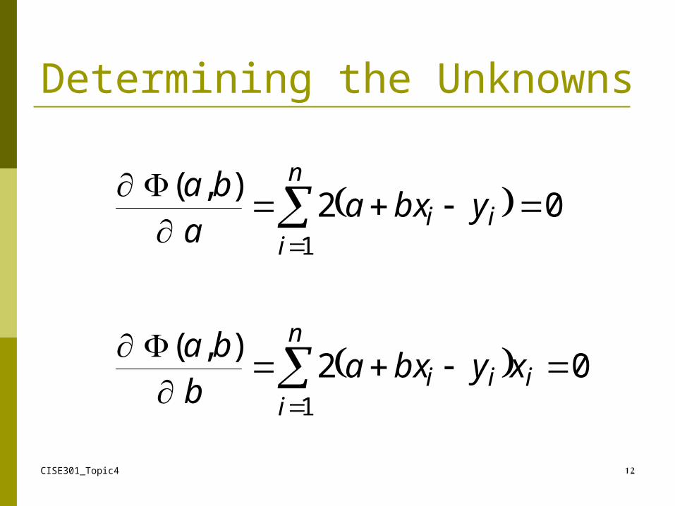
Determining the Unknowns

02),(

02),(

1

1

i

n

iii

n

iii

xybxab

ba

ybxaa

ba

CISE301_Topic4 13

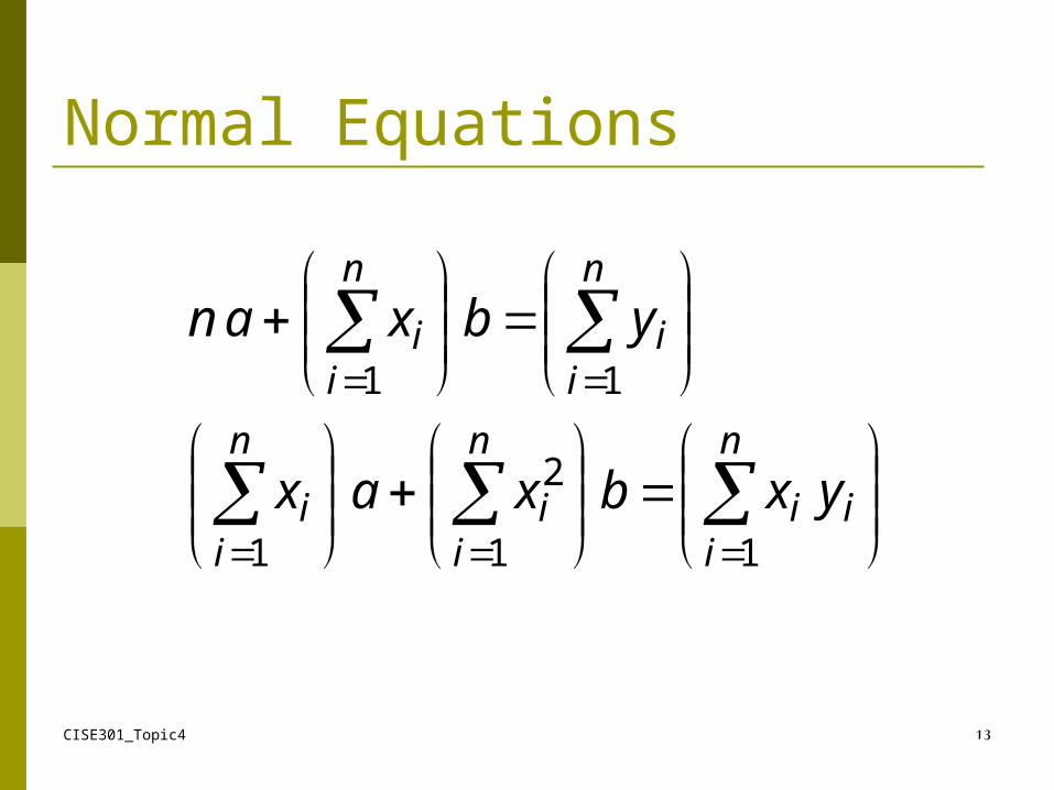
Normal Equations

n

iii

n

ii

n

ii

n

ii

n

ii

yxbxax

ybxan

11

2

1

11

CISE301_Topic4 14

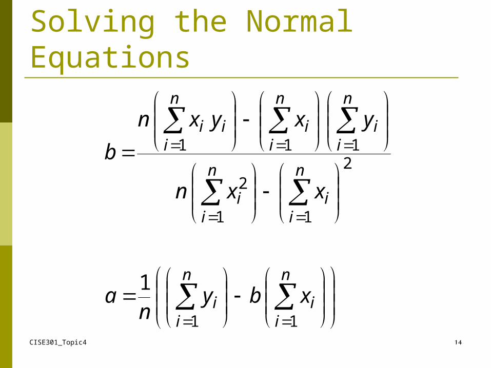
Solving the Normal Equations

n

ii

n

ii

n

ii

n

ii

n

ii

n

ii

n

iii

xbyn

a

xxn

yxyxn

b

11

2

11

2

111

1

CISE301_Topic4 15

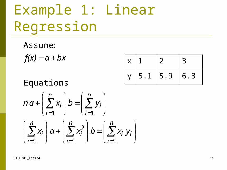
Example 1: Linear Regression

n

iii

n

ii

n

ii

n

ii

n

ii

yxbxax

ybxan

bxaf(x)

11

2

1

11

:Equations

:Assume

x 1 2 3

y 5.1 5.9 6.3

CISE301_Topic4 16

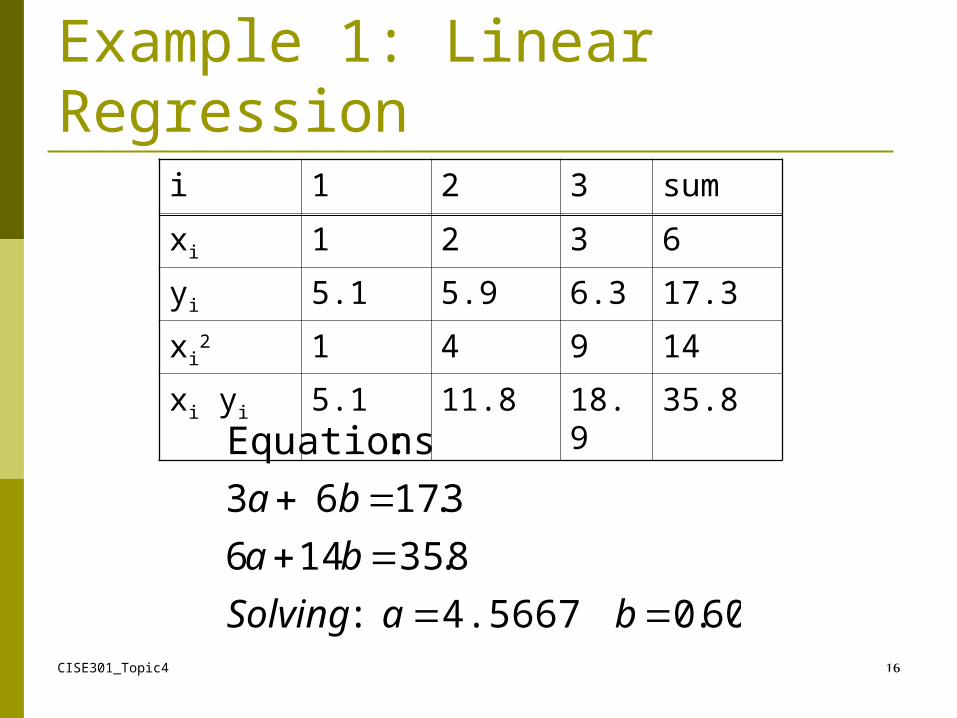
Example 1: Linear Regression

i 1 2 3 sum

xi 1 2 3 6

yi 5.1 5.9 6.3 17.3

xi2 1 4 9 14

xi yi 5.1 11.8 18.9 35.8

60.04.5667:

8.35146

3.1763

:Equations

baSolving

ba

ba

CISE301_Topic4 17

Multiple Linear Regression

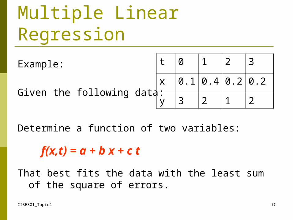
Example:

Given the following data:

Determine a function of two variables:

f(x,t) = a + b x + c t

That best fits the data with the least sum of the square of errors.

t 0 1 2 3

x 0.1 0.4 0.2 0.2

y 3 2 1 2

CISE301_Topic4 18

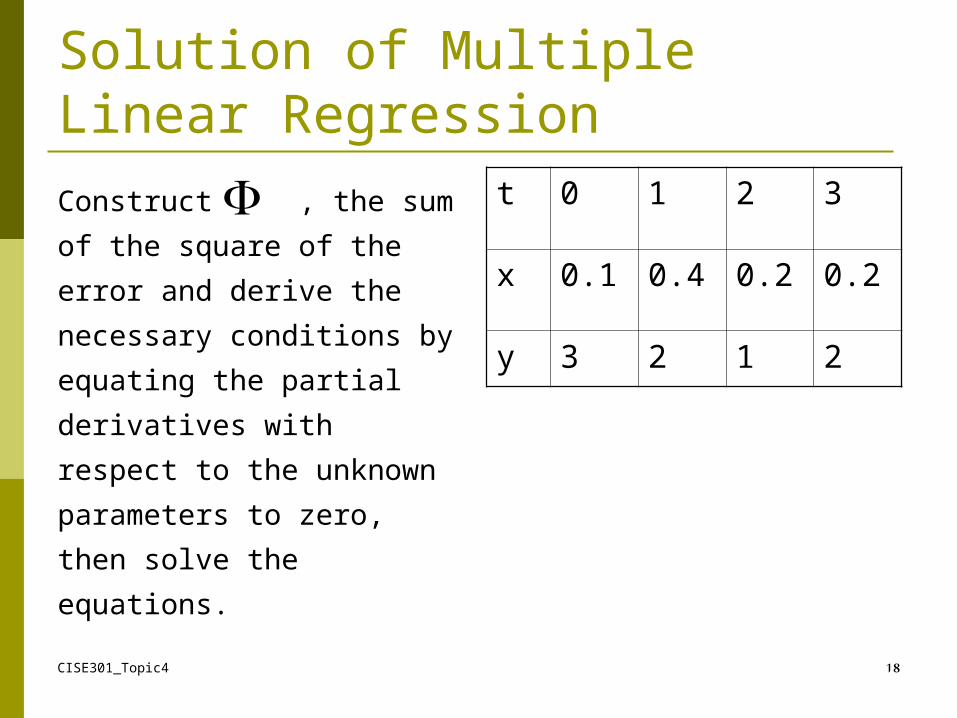
Solution of Multiple Linear Regression

Construct , the sum of

the square of the error

and derive the

necessary conditions by

equating the partial

derivatives with respect

to the unknown

parameters to zero, then

solve the equations.

t 0 1 2 3

x 0.1 0.4 0.2 0.2

y 3 2 1 2

CISE301_Topic4 19

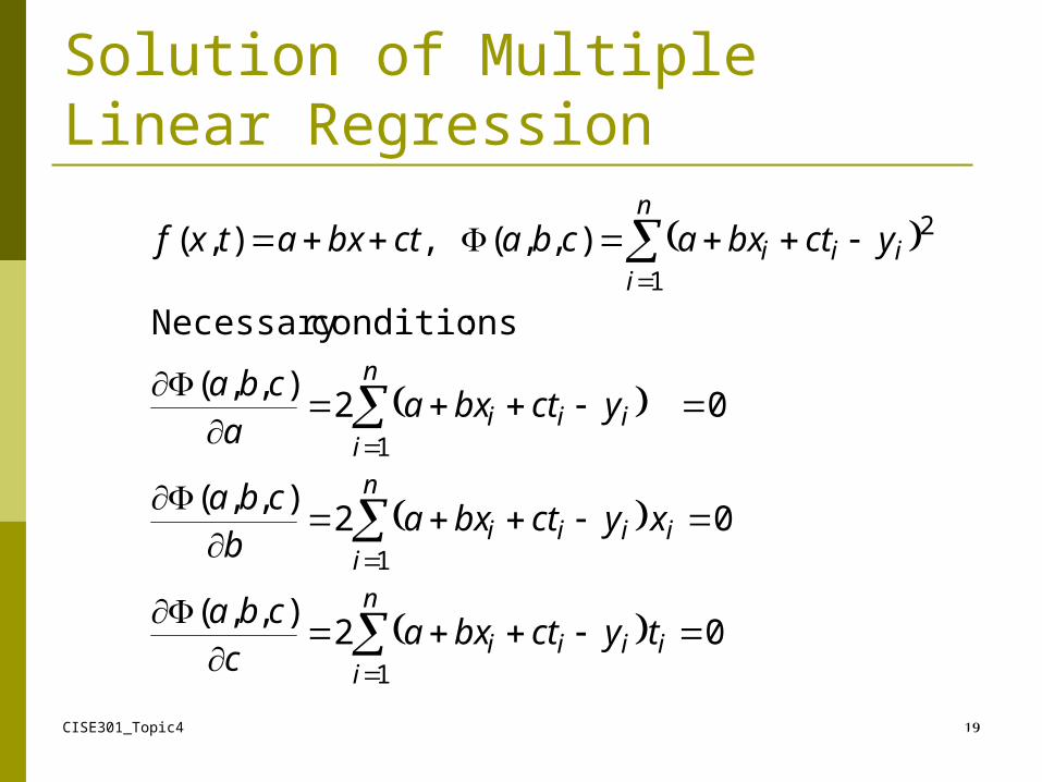
Solution of Multiple Linear Regression

02),,(

02),,(

02),,(

:conditions Necessary

),,( ,),(

1

1

1

1

2

i

n

iiii

i

n

iiii

n

iiii

n

iiii

tyctbxac

cba

xyctbxab

cba

yctbxaa

cba

yctbxacbactbxatxf

CISE301_Topic4 20

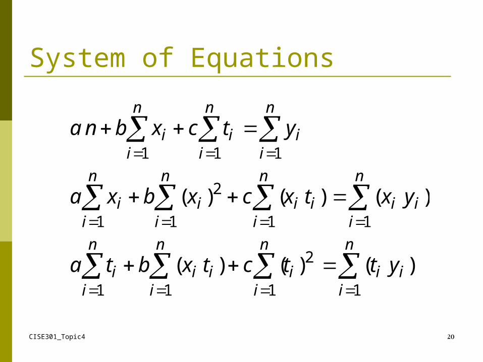
System of Equations

) ()() (

) () ()(

1

2

1 11

11 1

2

1

11 1

n

iiii

n

i

n

iii

n

ii

n

iiiii

n

i

n

ii

n

ii

n

ii

n

i

n

iii

yttctxbta

yxtxcxbxa

ytcxbna

CISE301_Topic4 21

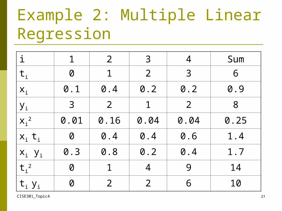
Example 2: Multiple Linear Regression

i 1 2 3 4 Sum

ti 0 1 2 3 6

xi 0.1 0.4 0.2 0.2 0.9

yi 3 2 1 2 8

xi2 0.01 0.16 0.04 0.04 0.25

xi ti 0 0.4 0.4 0.6 1.4

xi yi 0.3 0.8 0.2 0.4 1.7

ti2 0 1 4 9 14

ti yi 0 2 2 6 10

CISE301_Topic4 22

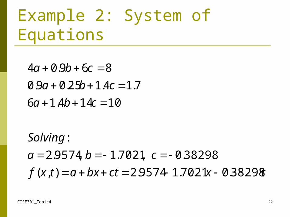
Example 2: System of Equations

txctbxatxf

cba

Solving

cba

cba

cba

38298.0 7021.19574.2),(

38298.0 ,7021.1 ,9574.2

:

10144.16

7.14.125.09.0

869.0 4

CISE301_Topic4 23

Lecture 19Nonlinear Least Squares

Problems

Examples of Nonlinear Least Squares Solution of Inconsistent Equations Continuous Least Square Problems

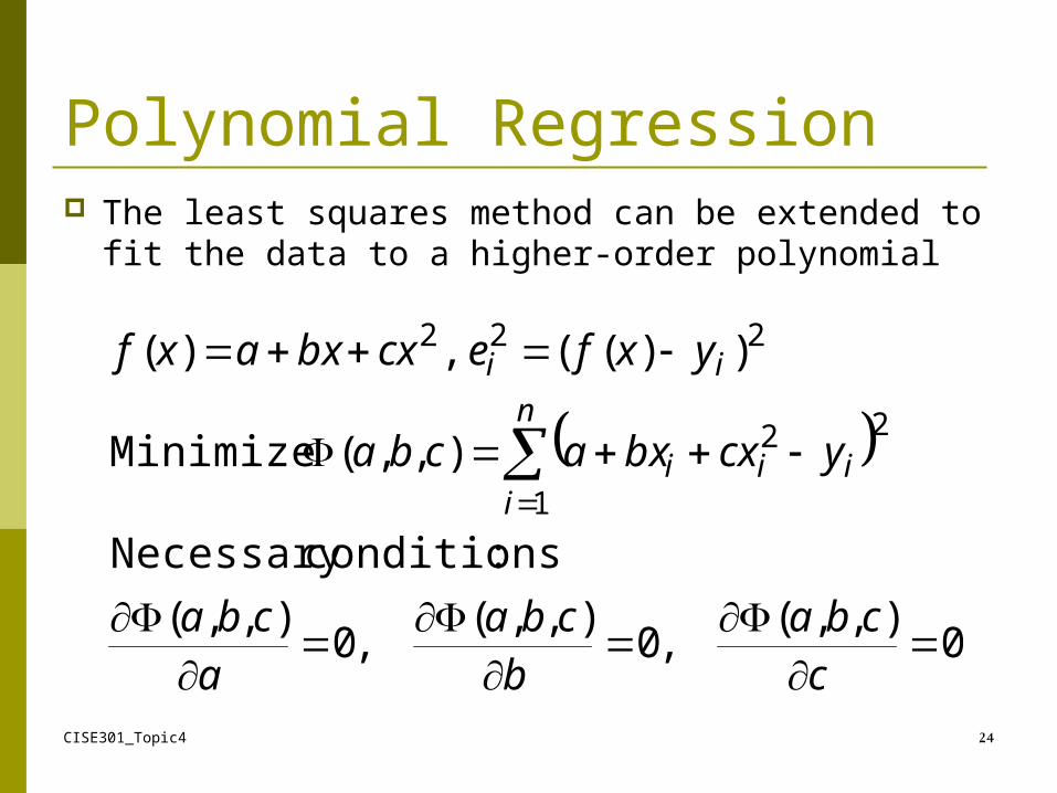
Polynomial Regression The least squares method can be extended to fit

the data to a higher-order polynomial

CISE301_Topic4 24

0),,(

,0),,(

,0),,(

:conditions Necessary

),,( Minimize

))(( ,)(

1

22

222

ccba

bcba

acba

ycxbxacba

yxfecxbxaxfn

iiii

ii

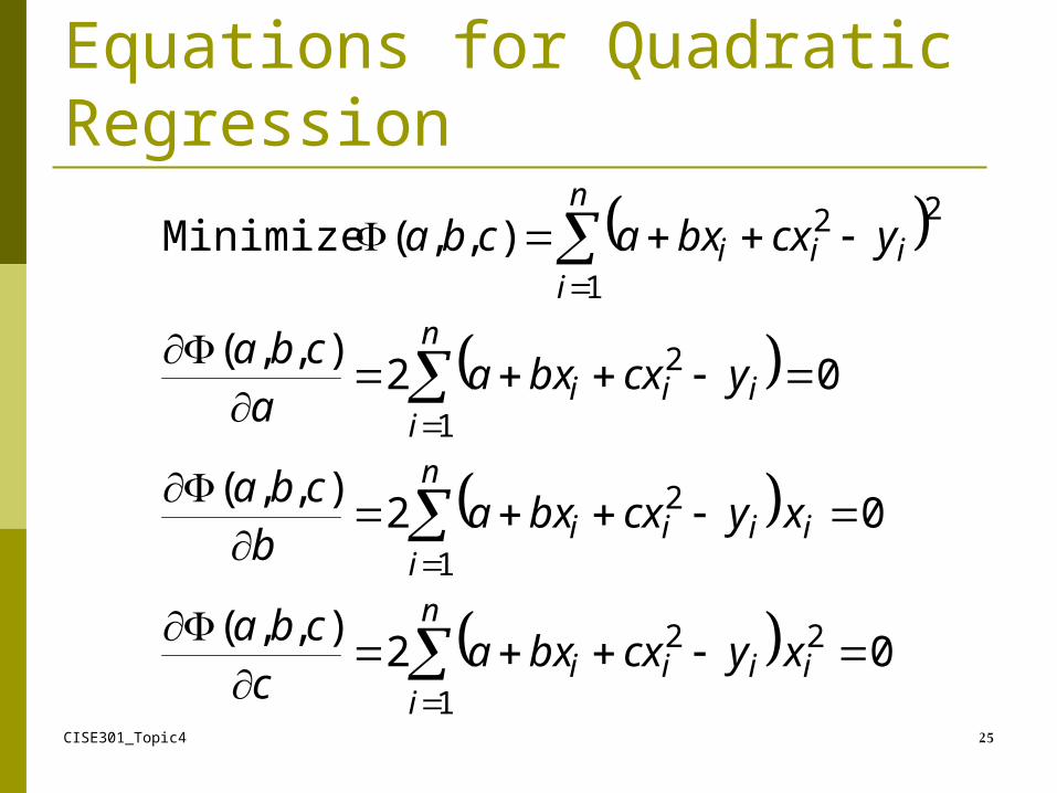
Equations for Quadratic Regression

CISE301_Topic4 25

0 2),,(

0 2),,(

02),,(

),,( Minimize

2

1

2

1

2

1

2

1

22

i

n

iiii

i

n

iiii

n

iiii

n

iiii

xycxbxac

cba

xycxbxab

cba

ycxbxaa

cba

ycxbxacba

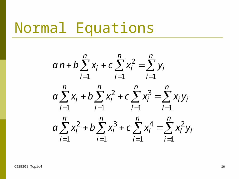
Normal Equations

CISE301_Topic4 26

n

iii

n

ii

n

ii

n

ii

n

iii

n

ii

n

ii

n

ii

n

ii

n

ii

n

ii

yxxcxbxa

yxxcxbxa

yxcxbna

1

2

1

4

1

3

1

2

11

3

1

2

1

11

2

1

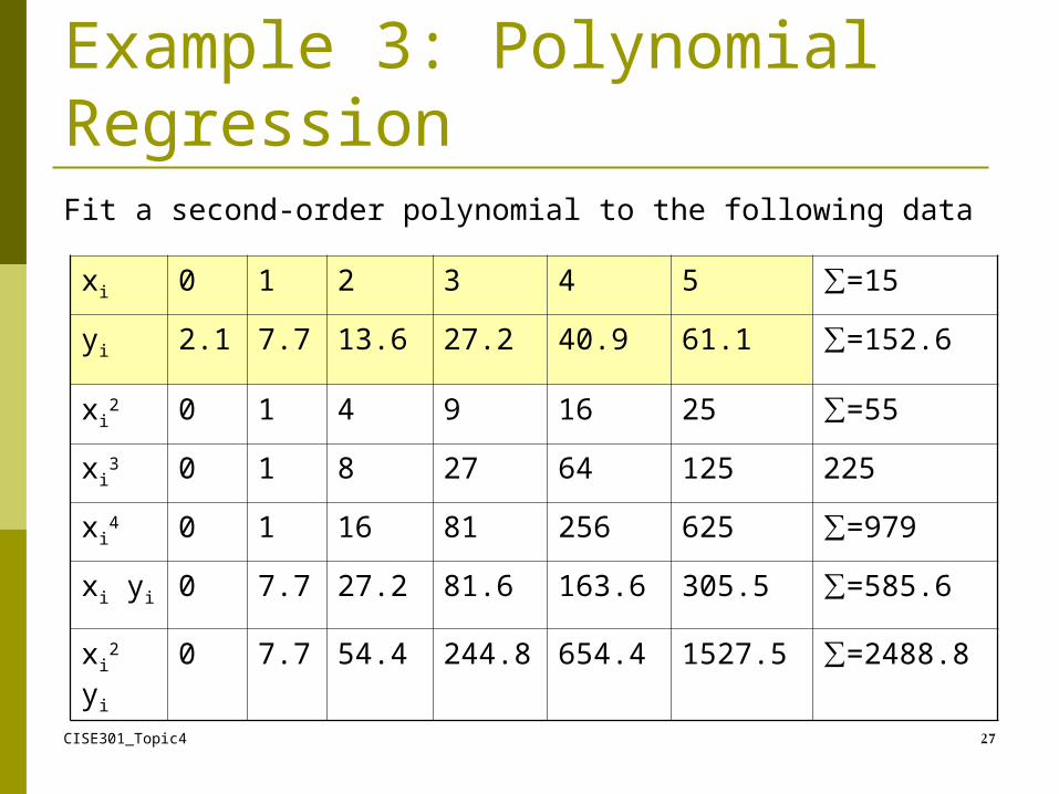
Example 3: Polynomial RegressionFit a second-order polynomial to the following data

CISE301_Topic4 27

xi 0 1 2 3 4 5 ∑=15

yi 2.1 7.7 13.6 27.2 40.9 61.1 ∑=152.6

xi2 0 1 4 9 16 25 ∑=55

xi3 0 1 8 27 64 125 225

xi4 0 1 16 81 256 625 ∑=979

xi yi 0 7.7 27.2 81.6 163.6 305.5 ∑=585.6

xi2 yi 0 7.7 54.4 244.8 654.4 1527.5 ∑=2488.8

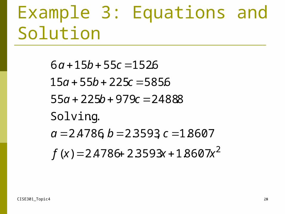
Example 3: Equations and Solution

CISE301_Topic4 28

2 8607.1 3593.24786.2)(

8607.1 ,3593.2 ,4786.2

. . . Solving

8.2488 979 225 55

6.585 225 55 15

6.152 55 15 6

xxxf

cba

cba

cba

cba

CISE301_Topic4 29

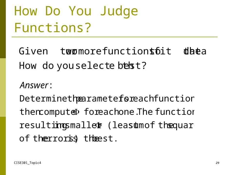
How Do You Judge Functions?

best? eselect thyou do How

data, fit the tofunctions moreor Given two

best. theis errors) theof

squares theof sum(least smaller in resulting

function The one. eachfor compute then

function, eachfor parameters theDetermine

:

Answer

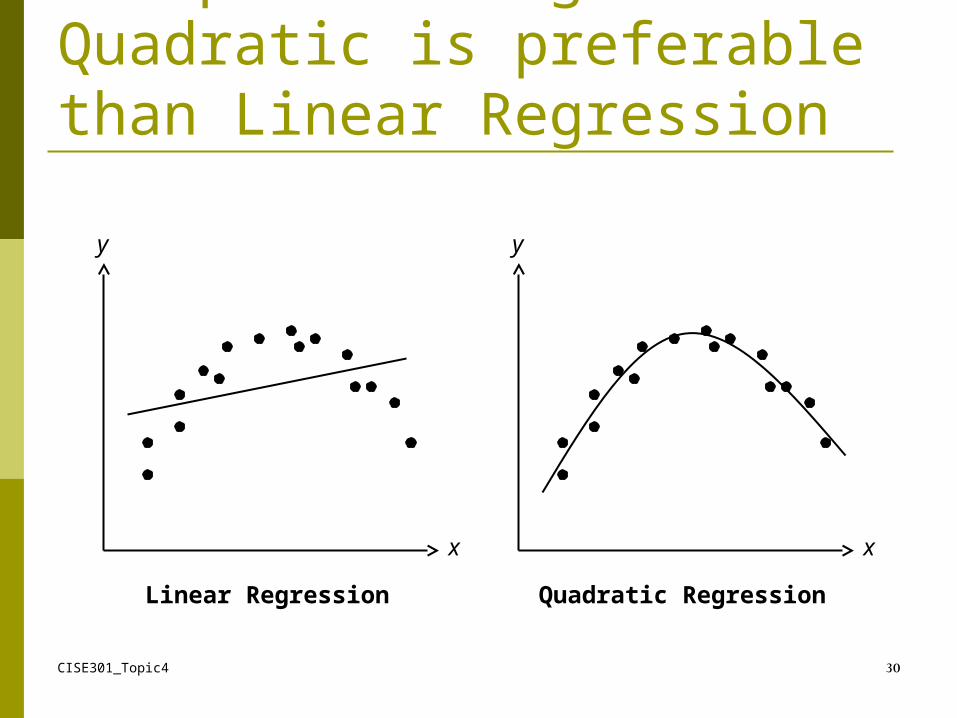
Example showing that Quadratic is preferable than Linear Regression

CISE301_Topic4 30

x

y

Quadratic Regression

x

y

Linear Regression

CISE301_Topic4 31

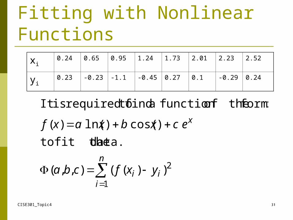
Fitting with Nonlinear Functions

n

iii

x

yxfcba

ecxbxaxf

1

2))((),,(

data. fit the to

)cos()ln()(

:form theof functiona find torequired isIt

xi0.24 0.65 0.95 1.24 1.73 2.01 2.23 2.52

yi0.23 -0.23 -1.1 -0.45 0.27 0.1 -0.29 0.24

CISE301_Topic4 32

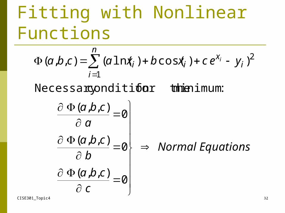
Fitting with Nonlinear Functions

EquationsNormal

ccba

bcba

acba

yecxbxacban

ii

xii

i

0),,(

0),,(

0),,(

:minimum for the condition Necessary

) )cos( )ln((),,(1

2

CISE301_Topic4 33

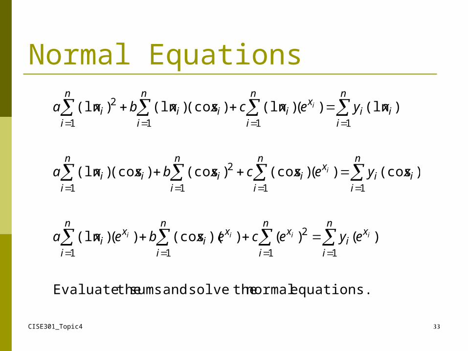
Normal Equations

equations. normal thesolve and sums theEvaluate

)()())((cos)()(ln

)(cos)()(cos)(cos)(cos)(ln

)(ln)()(ln)(cos)(ln)(ln

11

2

11

111

2

1

1111

2

iiii

i

i

xn

ii

n

i

xn

i

xi

xn

ii

n

iii

xn

ii

n

iii

n

ii

n

iii

xn

iii

n

ii

n

ii

eyecexbexa

xyexcxbxxa

xyexcxxbxa

CISE301_Topic4 34

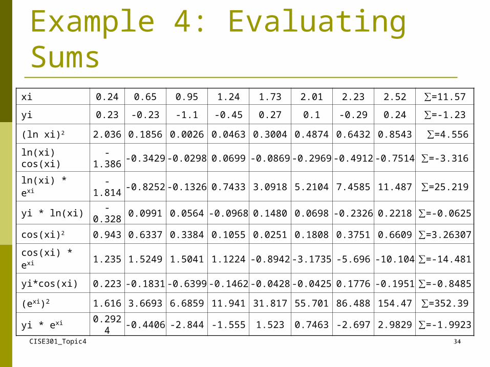
Example 4: Evaluating Sums

xi 0.24 0.65 0.95 1.24 1.73 2.01 2.23 2.52 ∑=11.57

yi 0.23 -0.23 -1.1 -0.45 0.27 0.1 -0.29 0.24 ∑=-1.23

(ln xi)2 2.036 0.1856 0.0026 0.0463 0.3004 0.4874 0.6432 0.8543 ∑=4.556

ln(xi) cos(xi) -1.386 -0.3429 -0.0298 0.0699 -0.0869 -0.2969 -0.4912 -0.7514 ∑=-3.316

ln(xi) * exi -1.814 -0.8252 -0.1326 0.7433 3.0918 5.2104 7.4585 11.487 ∑=25.219

yi * ln(xi) -0.328 0.0991 0.0564 -0.0968 0.1480 0.0698 -0.2326 0.2218 ∑=-0.0625

cos(xi)2 0.943 0.6337 0.3384 0.1055 0.0251 0.1808 0.3751 0.6609 ∑=3.26307

cos(xi) * exi 1.235 1.5249 1.5041 1.1224 -0.8942 -3.1735 -5.696 -10.104 ∑=-14.481

yi*cos(xi) 0.223 -0.1831 -0.6399 -0.1462 -0.0428 -0.0425 0.1776 -0.1951 ∑=-0.8485

(exi)2 1.616 3.6693 6.6859 11.941 31.817 55.701 86.488 154.47 ∑=352.39

yi * exi 0.2924 -0.4406 -2.844 -1.555 1.523 0.7463 -2.697 2.9829 ∑=-1.9923

CISE301_Topic4 35

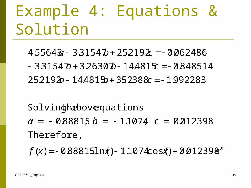
Example 4: Equations & Solution

xexxxf

, c , b a

cba

cba

cba

012398.0)cos( 1074.1)ln( 88815.0)(

Therefore,

012398.01074.188815.0

:equations above theSolving

992283.1 388.352 4815.14 2192.25

848514.0 4815.14 26307.3 31547.3

062486.0 2192.25 31547.3 55643.4

CISE301_Topic4 36

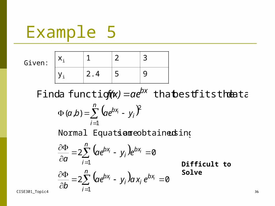
data. thefitsbest that functiona Find bxaef(x)

02

02

:using obtained are s EquationNormal

),(

1

1

1

2

ii

ii

i

bxi

n

ii

bx

bxn

ii

bx

n

ii

bx

exayaeb

eyaea

yaeba

Example 5

Given:xi 1 2 3

yi 2.4 5 9

Difficult to Solve

CISE301_Topic4 37

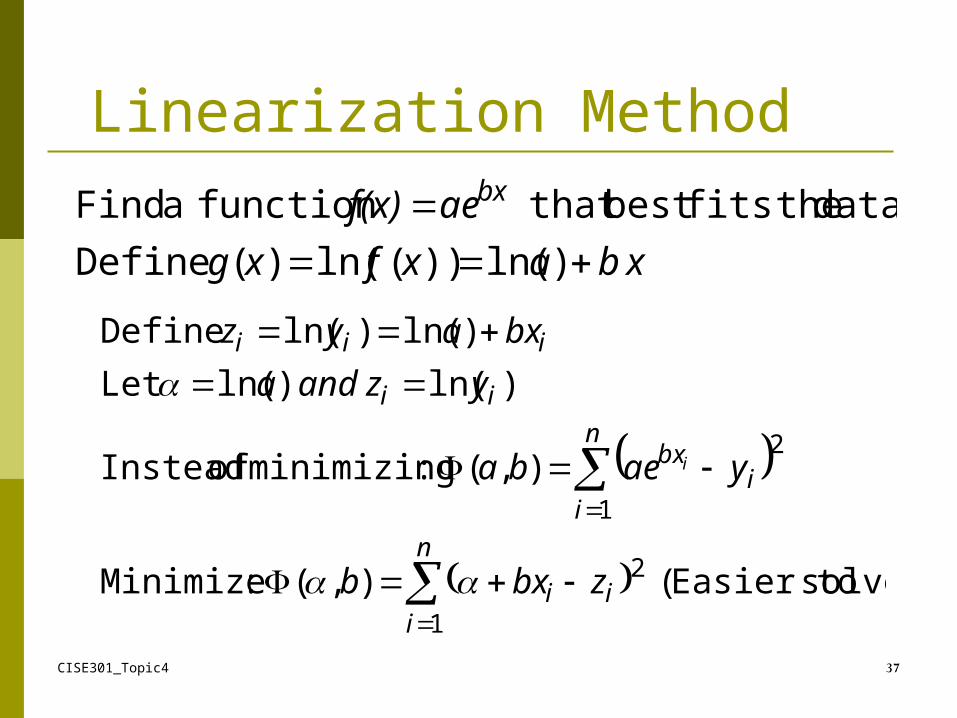
xbaxfxg

aef(x) bx

)ln())(ln()( Define

data. thefitsbest that functiona Find

solve) Easier to(),( :Minimize

),( :minimizing of Instead

)ln()ln(Let

)ln()ln( Define

1

2

1

2

n

iii

n

ii

bx

ii

iii

zbxb

yaeba

yzanda

bxayz

i

Linearization Method

CISE301_Topic4 38

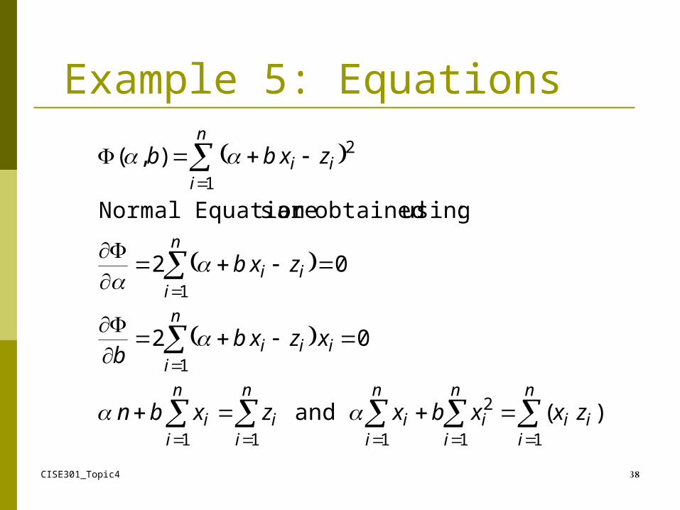
n

iii

n

ii

n

ii

n

ii

n

ii

i

n

iii

n

iii

n

iii

zxxbxzxbn

xzxbb

zxb

zxbb

11

2

111

1

1

1

2

) ( and

0 2

0 2

:using obtained are s EquationNormal

),(

Example 5: Equations

CISE301_Topic4 39

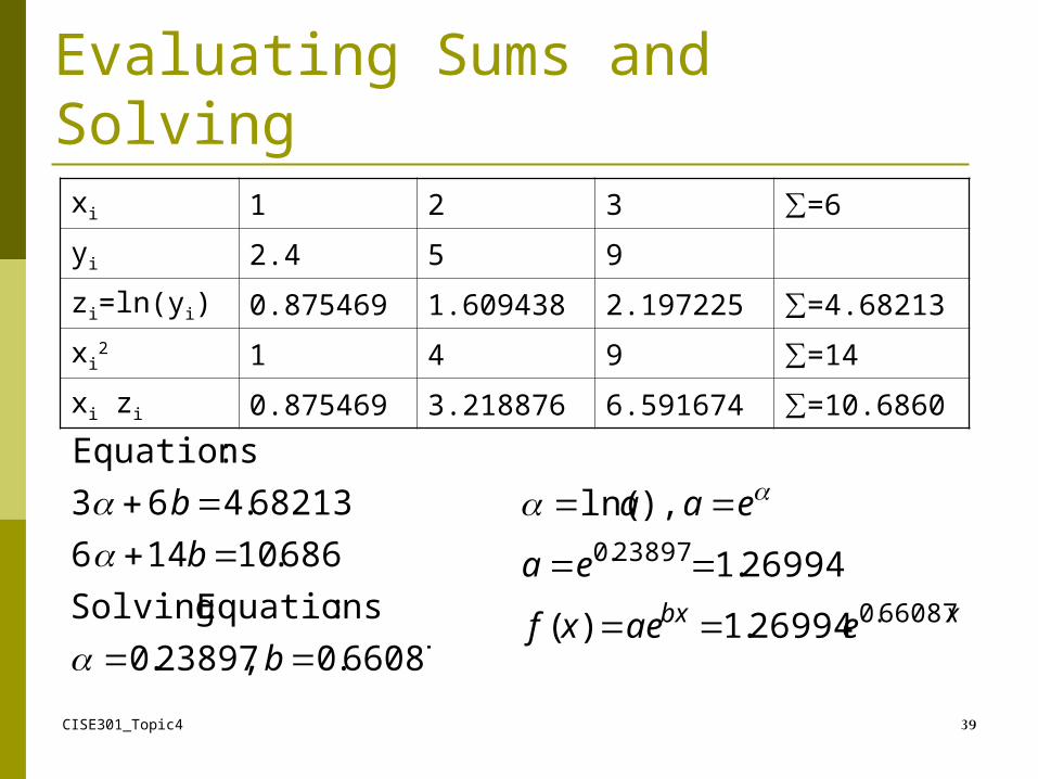
66087.0 ,23897.0

: EquationsSolving

686.10 14 6

68213.4 6 3

:Equations

b

b

b

Evaluating Sums and Solvingxi 1 2 3 ∑=6

yi 2.4 5 9

zi=ln(yi) 0.875469 1.609438 2.197225 ∑=4.68213

xi2 1 4 9 ∑=14

xi zi 0.875469 3.218876 6.591674 ∑=10.6860

xbx eaexf

ea

eaa

66087.0

23897.0

26994.1)(

26994.1

),ln(