Cisneros-Magañia, Rafael and Medina, Aurelio and Anaya-Lara, Olimpo

(2018) Time-domain voltage sag state estimation based on the

unscented Kalman filter for power systems with nonlinear components.

Energies. ISSN 1996-1073 (In Press) ,

This version is available at https://strathprints.strath.ac.uk/64176/

Strathprints is designed to allow users to access the research output of the University of

Strathclyde. Unless otherwise explicitly stated on the manuscript, Copyright © and Moral Rights

for the papers on this site are retained by the individual authors and/or other copyright owners.

Please check the manuscript for details of any other licences that may have been applied. You

may not engage in further distribution of the material for any profitmaking activities or any

commercial gain. You may freely distribute both the url (https://strathprints.strath.ac.uk/) and the

content of this paper for research or private study, educational, or not-for-profit purposes without

prior permission or charge.

Any correspondence concerning this service should be sent to the Strathprints administrator:

strathprints@strath.ac.uk

The Strathprints institutional repository (https://strathprints.strath.ac.uk) is a digital archive of University of Strathclyde research

outputs. It has been developed to disseminate open access research outputs, expose data about those outputs, and enable the

management and persistent access to Strathclyde's intellectual output.

Energies 2018, 11, x; doi: FOR PEER REVIEW www.mdpi.com/journal/energies

Article 1

Time-domain voltage sag state estimation based on 2

the unscented Kalman filter for power systems with 3

nonlinear components 4

Rafael Cisneros-Magaña 1, Aurelio Medina 1, * and Olimpo Anaya-Lara 2 5

1 División de Estudios de Posgrado, Facultad de Ingeniería Eléctrica, Universidad Michoacana de San 6

Nicolás de Hidalgo, Av. Francisco J. Múgica S/N, Morelia, Michoacán, 58030, México; 7

rcisneros@dep.fie.umich.mx (R.C.); amedinr@gmail.com (A.M.) 8 2 Institute for Energy and Environment, Department of Electronic and Electrical Engineering, University of 9

Strathclyde, 204 George Street, Glasgow, Scotland, UK; olimpo.anaya-lara@strath.ac.uk (O.A.) 10

* Correspondence: amedinr@gmail.com; Tel.: +52-443-327-9728 11

Received: date; Accepted: date; Published: date 12

Abstract: This paper proposes a time-domain methodology based on the unscented Kalman filter 13

to estimate voltage sags and their characteristics, such as magnitude and duration in power systems 14

represented by nonlinear models. Partial and noisy measurements from the electrical network with 15

nonlinear loads, used as data, are assumed. The characteristics of voltage sags can be calculated in 16

a discrete form with the unscented Kalman filter to estimate all the busbar voltages; being possible 17

to determine the rms voltage magnitude and the voltage sag starting and ending time, respectively. 18

Voltage sag state estimation results can be used to obtain the power quality indices for monitored 19

and unmonitored busbars in the power grid and to design adequate mitigating techniques. The 20

proposed methodology is successfully validated against the results obtained with the time-domain 21

system simulation for the power system with nonlinear components, being the normalized root 22

mean square error less than 3%. 23

Keywords: Nonlinear dynamic system; power quality; power system simulation; state estimation; 24

unscented Kalman filter; voltage fluctuation 25

26

1. Introduction 27

Power quality (PQ) is an important operation issue of any power system. Utilities must comply 28

with strict standards, relating primarily harmonics, transients and voltage sags [1-4]. PQ depends on 29

the power supply, the transmission and distribution systems and the electrical load condition. 30

Voltage sags are among the adverse PQ effects; they can cause malfunction of electronic loads, and 31

can reset voltage-sensitive loads [5-6]. The voltage sags characteristics in magnitude and duration are 32

necessary to determine their effect in the grid and its loads. They constitute the majority of PQ 33

problems, representing about 60% of them [7-8]. Among the problems that the nonlinear electrical 34

components introduce to the power grid is the increase of harmonic distortion, which is an important 35

effect to mitigate. Voltage sags have increased due to the use of nonlinear varying loads such as 36

power electronic devices, smelters, arc furnaces and electric welders, the starting of large electrical 37

loads, switching transients, connection of transformers and transmission lines, network faults, 38

lightning strikes, network switching operations, among others [9]. 39

Kalman filter (KF) and the least squares method have been used to estimate the voltage 40

fluctuations in linear power systems [10-13]. PQ state estimation based on the KF uses a linear model, 41

partial and noisy measurements from the system. In [14] the number of sags is estimated using a 42

limited number of monitored busbars, recording the number of voltage sags during a determined 43

period. 44

Energies 2018, 11, x FOR PEER REVIEW 2 of 20

This research work proposes as an innovation, an alternative methodology based on the 45

unscented Kalman filter (UKF) to perform the voltage sags state estimation (VSSE) in nonlinear load 46

power networks; this method can also be applied to nonlinear micro grids. The VSSE determines the 47

magnitude, duration and beginning-ending time of sags, with an observable system condition for the 48

busbars voltages using the available measurements. 49

The KF has been applied to estimate harmonics and voltage transients in a signal [15], KF gain 50

can be modified during the state estimation to reduce the estimation error [16], both references assess 51

linear cases; [17] has proposed the UKF to detect sags in a voltage waveform. In this work, the UKF 52

is extended to the nonlinear case to solve the time-domain VSSE, to estimate voltage sags in all 53

busbars of a power system including nonlinear components. The UKF makes use of a power grid 54

nonlinear model and noisy measurements from the same electrical network to estimate all the busbar 55

voltages. 56

The extended Kalman filter (EKF) can be also applied to solve the nonlinear state estimation. 57

The UKF error is slightly smaller when compared to the EKF error. This state estimation error 58

increases in the filters when sudden variations are present, both being of about the same accuracy. 59

The EKF can lead to divergence more easily than UKF, which shows good numerical stability 60

properties. 61

The state estimation receives measurements from the power network, through a wide area 62

measurement system (WAMS) and estimates the state vector, using algorithms such as the UKF. 63

Practical implementation of the time-domain state estimation can be achieved with measuring 64

instruments and data acquisition cards, capable of recording the voltage and current waveforms 65

synchronously during several cycles, e.g. using the global positioning system (GPS) to time stamp 66

the measurements [18-21]. The use of adequate communication channels like especially dedicated 67

optical fibre links, allows to the measurements be sent to the control centre with high data updating 68

rate, where they are received and numerically processed using computational systems with sufficient 69

memory and adequate capability [9]. 70

Measurement technology for VSSE is currently limited, making the system underdetermined, 71

due to economic reasons. The VSSE presents different problems from those of the traditional power 72

system state estimation, where redundancy of measurements is possible [22]. 73

The VSSE has been assessed in the frequency domain [14, 23]. In this work, the UKF is proposed 74

as an alternative method to obtain the time-domain VSSE. This approach makes possible the use of 75

nonlinear models to represent more accurately the power system components and to obtain the 76

results with a low state estimation error. The state estimation obtains the global or total system state 77

that can be used to take corrective actions to mitigate the adverse effects of voltage sags, such as the 78

network configuration change or control of flexible alternating current transmission system (FACTS) 79

devices, e.g. the static synchronous compensator (STATCOM). 80

The time-domain UKF state estimation methodology can be used not only to estimate voltage 81

sags but also to estimate over voltages, over currents or electromagnetic transients. The main 82

objective of this work is to apply the UKF to obtain the VSSE, by addressing the dynamics of the 83

nonlinear electrical networks and by estimating and delimiting the voltage sags in the time-domain. 84

The case studies address short circuit faults and transient load conditions. The results are validated 85

against the actual time-domain response of the power grid. 86

2. Dynamic state estimation 87

The network model can be a set of first order differential equations to describe the dynamic state 88

performance. The dynamic estimation data are the grid model with its inputs and a measurement set 89

of selected outputs from the system during a determined number of cycles to define the measurement 90

equation. 91

The KF dynamically follows the variations in the states, i.e. currents and voltages, detecting 92

changes in the voltage waveform within less than half of a cycle and it is a good tool for instantaneous 93

tracking and detection of voltage sags [24-25]. 94

Energies 2018, 11, x FOR PEER REVIEW 3 of 20

The KF solves the dynamic estimation, due to its recursive process [26-27]; being applied in 95

linear cases. The UKF solves the dynamic estimation in nonlinear cases. In this work, the UKF 96

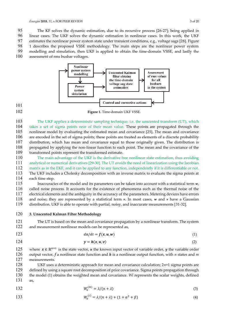
estimates the nonlinear power system state under transient conditions, e.g., voltage sags [28]. Figure 97

1 describes the proposed VSSE methodology. The main steps are the nonlinear power system 98

modelling and simulation, then UKF is applied to obtain the time-domain VSSE, and lastly the 99

assessment of rms busbar voltages. 100

101

Figure 1. Time-domain UKF VSSE. 102

The UKF applies a deterministic sampling technique; i.e. the unscented transform (UT), which 103

takes a set of sigma points near of their mean value. These points are propagated through the 104

nonlinear model by evaluating the estimated mean and covariance [25]. The mean and covariance 105

are encoded in the set of sigma points; these points are treated as elements of a discrete probability 106

distribution, which has mean and covariance equal to those originally given. The distribution is 107

propagated by applying the non-linear function to each point. The mean and the covariance of the 108

transformed points represent the transformed estimate. 109

The main advantage of the UKF is the derivative free nonlinear state estimation, thus avoiding 110

analytical or numerical derivatives [29-30]. The UT avoids the need of linearization using the Jacobian 111

matrix as in the EKF, and it can be applied to any function, independently if it is differentiable or not. 112

The UKF includes a Cholesky decomposition with an inverse matrix to evaluate the sigma points at 113

each time step. 114

Inaccuracies of the model and its parameters can be taken into account with a statistical term w, 115

called noise process. It accounts for the existence of phenomena such as the thermal noise of the 116

electrical elements and the ambiguity in the accuracy of the parameters. Metering devices have errors 117

and noise; they are represented by a statistical term v. In most cases, w and v have a Gaussian 118

distribution. UKF is able to operate with partial, noisy, and inaccurate measurements [31-32]. 119

3. Unscented Kalman Filter Methodology 120

The UT is based on the mean and covariance propagation by a nonlinear transform. The system 121

and measurement nonlinear models can be represented as, 122 穴姉【穴建 噺 讃岫姉┸ 四┸ 始岻 (1) 123 姿 噺 酸岫姉┸ 四┸ 士岻 (2) 124

where 姉 樺 温津抜怠 is the state vector, u the known input vector of variable order, y the variable order 125

output vector, f a nonlinear state function and h is a nonlinear output function, with n states and m 126

measurements. 127

UKF uses a deterministic approach for mean and covariance calculation; 2n+1 sigma points are 128

defined by using a square root decomposition of prior covariance. Sigma points propagation through 129

the model (1) obtains the weighted mean and covariance. Wi represents the scalar weights, defined 130

as, 131 激待岫陳岻 噺 膏【岫券 髪 膏岻 (3) 132 激待岫頂岻 噺 膏【岫券 髪 膏岻 髪 岫な 髪 糠態 髪 紅岻 (4) 133

Energies 2018, 11, x FOR PEER REVIEW 4 of 20

激沈岫陳岻 噺 激沈岫頂岻 噺 な【岫に岫券 髪 膏岻岻┸ 件 噺 な┸ ┼ ┸ に券 (5) 134 膏 噺 糠態岫券 髪 腔岻 伐 券 (6) 135 紘 噺 ヂ券 髪 膏 (7) 136

where ゆ and ま are scaling parameters, ぼ and ゅ determine the spread of sigma points; ぽ is associated 137

with the distribution of x. If Gaussian ぽ=2 is optimal, ぼ=10-3 and ゅ=0 are normal values [30]. 138

UT takes the sigma points with their mean and covariance values, and transform them by 139

applying the nonlinear function f, and then the mean and covariance can be calculated for the 140

transformed points. A weight Wi is assigned to each point. 141

UKF defines the n-state discrete-time nonlinear system from (1) and (2) as, 142 姉賃袋怠 噺 讃岫姉賃 ┸ 四賃┸ 始賃 ┸ 嗣賃岻 (8) 143 姿賃 噺 酸岫姉賃 ┸ 四賃┸ 士賃┸ 嗣賃岻 (9) 144 始賃 漢 軽岫ど┸ 晒賃岻 (10) 145 士賃 漢 軽岫ど┸ 三賃岻 (11) 146

Process noise w and measurement noise v are assumed stationary, zero-averaged and 147

uncorrelated, 晒 樺 温津抜津 and 三 樺 温陳抜陳 are the covariance matrices for noises w and v, respectively. 148

UKF applies the following steps: 149

a) Initialization, k=0. 150 姉赴待袋 噺 撮岫捲待岻 (12) 151 皿待袋 噺 撮岷岫捲待 伐 姉赴待袋岻岫捲待 伐 姉赴待袋岻脹 峅 (13) 152

E is the expected value, P is the error covariance matrix, + indicates update estimate or a 153

posteriori estimate and む project estimate or a priori estimate. Subscripts k and k-1 denote time 154

instants t=k┡t and t=(k-ｱ《┡t╇やrespectively╇や┡t is the time step. 155

b) Sigma points assessment in matrix form by columns: 156 璽賃貸怠 噺 岷 姉赴賃貸怠 姉赴賃貸怠 髪 紘紐皿賃貸怠 姉赴賃貸怠 伐 紘紐皿賃貸怠 峅 (14) 157

c) Update time step k from k-1. 158 璽賃孕賃貸怠茅 噺 讃岷璽賃貸怠┸ 四賃貸怠峅 (15) 159

姉赴賃貸 噺 デ 激沈岫陳岻璽沈┸賃孕賃貸怠茅態津沈退待 (16) 160

皿賃貸 噺 デ 激沈岫頂岻態津沈退待 峙璽沈┸賃孕賃貸怠茅 伐 姉赴賃貸峩 峙璽沈┸賃孕賃貸怠茅 伐 姉赴賃貸峩脹 髪 晒賃 (17) 161

璽賃孕賃貸怠 噺 範 姉赴賃貸 姉赴賃貸 髪 紘紐皿賃貸 姉赴賃貸 伐 紘紐皿賃貸 飯 (18) 162

姿賃孕賃貸怠茅 噺 酸 峙璽賃孕賃貸怠峩 (19) 163

姿赴賃貸 噺 デ 激沈岫陳岻姿沈┸賃孕賃貸怠茅態津沈退待 (20) 164

Energies 2018, 11, x FOR PEER REVIEW 5 of 20

璽 matrix represents the sigma points; 璽茅 matrix represents the updated sigma points and 姿茅 165

the updated output vector with sigma points. 166

d) Evaluate the error covariance matrices as, 167 皿槻賦入槻賦入 噺 デ 激沈岫頂岻態津沈退待 峙姿沈┸賃孕賃貸怠茅 伐 姿赴賃貸峩 峙姿沈┸賃孕賃貸怠茅 伐 姿赴賃貸峩脹 髪 三賃 (21) 168

皿掴入槻入 噺 デ 激沈岫頂岻態津沈退待 峙璽沈┸賃孕賃貸怠茅 伐 姉赴賃貸峩 峙姿沈┸賃孕賃貸怠茅 伐 姿赴賃貸峩脹 (22) 169

e) UKF algorithm evaluates the filter gain Kk and updates the estimated state and the error 170

covariance matrix. 171 皐賃 噺 皿掴入槻入皿槻賦入槻賦入貸怠 (23) 172 姉赴賃袋 噺 姉赴賃貸 髪 皐賃岫姿賃 伐 姿赴賃貸岻 (24) 173 皿賃袋 噺 皿賃貸 髪 皐賃皿槻賦入槻賦入皐賃脹 (25) 174

The steps (b-d), equations (14)-(22), define the prediction stage, and the last step (e), equations 175

(23)-(25), defines the update stage, as in the KF algorithm [33-34]. The main objective of this work is 176

to use the UKF formulation to estimate the busbar voltage waveforms, mainly at unmonitored 177

busbars in the presence of voltage sags generated by faults and load transients. 178

Waveforms can be contaminated with noise, and the assumption of constant values for Q and R 179

is valid when the noise characteristics are constant, like its standard deviation and variance. If the 180

noise is varying, Q and R should be computed at each time step and an adaptive KF is a requirement 181

[16]. UKF algorithm tracks the time-varying model and noise through the on-line calculation of Q 182

and R. In this work, Q and R matrices are assumed constant, in order to mainly analyse the UKF 183

application to time-domain VSSE. 184

UKF identifies the interval where the sags are present, as well as their magnitude, with an 185

acceptable precision. By increasing the number of cycles, the UKF can identify the voltage 186

characteristics during fault transient periods. 187

The number of points per cycle is of important concern to evaluate the time-domain state 188

estimation with periodic signals. This number defines the sampling rate for the monitored signals. 189

The sampled waveform is a sequence of values taken at defined time intervals and represents the 190

measured variable. Interpolation can be used to adjust the number of points per cycle, linearly or 191

nonlinearly [35]. In addition, the interpolation should be used carefully with discrete signals to satisfy 192

the sampling theorem. The sampling rate defines the speed at which the input channels are sampled; 193

this rate is defined in samples per cycle. To detect transients, high sampling rates compared with the 194

fundamental frequency may be necessary [36]. 195

3.1 Rms value of discrete waveforms and normalized root mean square error. 196

The rms voltage magnitude can be determined by processing the discrete values for the voltage 197

waveform according to the used data window size and the sampling frequency. The rms voltage 198

magnitude Vrms for a discrete voltage signal can be calculated as, 199 撃追陳鎚岫件軽岻 噺 謬岫怠朝 デ 撃珍態沈朝珍退岫沈貸怠岻朝袋怠 岻 件 半 な (26) 200

Energies 2018, 11, x FOR PEER REVIEW 6 of 20

where Vj is the sample voltage j and N is the number of samples per cycle taken in the sampling 201

window; i is the sampled cycle. This expression can be applied to discrete voltage and current 202

waveforms [22]. 203

Normalized root mean square error (NRMSE) is used to validate the UKF-VSSE methodology; 204

this error evaluates the state estimation residual between actually observed values and the estimated 205

values; lower residual indicates less state estimation error. NRMSE is defined as, 206 軽迎警鯨継 噺 謬デ 岫姿赴禰貸姿禰岻鉄津椎津椎痛退怠 【岫姿陳銚掴 伐 姿陳沈津岻 (27) 207 姿赴 is the estimated vector, y is the real or actually observed vector and np the number of elements 208

of these vectors. 209

4. Case Studies 210

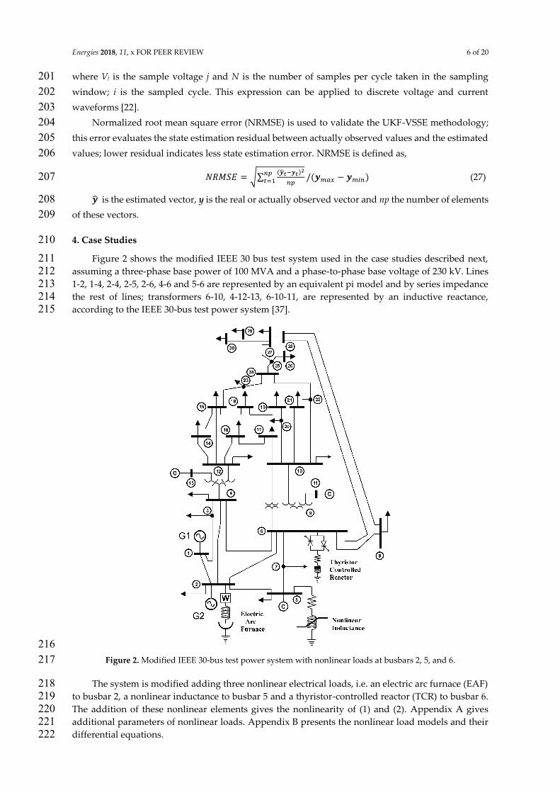
Figure 2 shows the modified IEEE 30 bus test system used in the case studies described next, 211

assuming a three-phase base power of 100 MVA and a phase-to-phase base voltage of 230 kV. Lines 212

1-2, 1-4, 2-4, 2-5, 2-6, 4-6 and 5-6 are represented by an equivalent pi model and by series impedance 213

the rest of lines; transformers 6-10, 4-12-13, 6-10-11, are represented by an inductive reactance, 214

according to the IEEE 30-bus test power system [37]. 215

216

Figure 2. Modified IEEE 30-bus test power system with nonlinear loads at busbars 2, 5, and 6. 217

The system is modified adding three nonlinear electrical loads, i.e. an electric arc furnace (EAF) 218

to busbar 2, a nonlinear inductance to busbar 5 and a thyristor-controlled reactor (TCR) to busbar 6. 219

The addition of these nonlinear elements gives the nonlinearity of (1) and (2). Appendix A gives 220

additional parameters of nonlinear loads. Appendix B presents the nonlinear load models and their 221

differential equations. 222

Energies 2018, 11, x FOR PEER REVIEW 7 of 20

Generators are modelled as voltage sources connected to busbars through a series inductance. 223

Linear electric loads are represented as constant impedances. Busbar voltages, line and load currents 224

are defined as state variables to obtain the state space model for the power network; the 225

measurements are function of these state variables. 226

The measurement locations are selected so that the busbar voltages are observable. Tables 1 and 227

2 show x and z vectors, respectively, to form the measurement equation by obtaining 103 228

measurements to estimate 110 state variables (n=110, m=103). The observation equation with this set 229

of measurements has an underdetermined condition, but all the busbar voltages are observable to 230

estimate the voltage sags. When busbar voltages are assessed and estimated other variables can be 231

calculated, i.e. line currents or the TCR current. 232

Table 1. State variable vector x 233

Description State variable

Line currents 1-41

Busbar voltages 42-71

Generator currents 72-77

Busbar load currents 78-106

Nonlinear inductor magnetic flux 107

EAF current and arc radius 108-109

TCR current 110

Table 2. Measurements vector z 234

Description Output variable

Line currents 1-38

Busbar voltages 42-68

Generator currents 72-77

Busbar load currents 78-106

Nonlinear inductor current 107

EAF real power 108-109

The EAF real power and the nonlinear inductance current are included as nonlinear functions 235

in the measurement equation (z=Hx) represented in the formulation by (2). 236

In the measurement matrix 殺 樺 温陳抜津, each measurement is associated with its corresponding 237

state variable (Table 2). The sampling frequency is at least 30.72 kHz, to obtain 512 samples per cycle, 238

for a fundamental frequency of 60 Hz [24]. 239

The conventional trapezoidal rule is used to solve the 110 first order ordinary differential 240

equations set. To represent the power system, busbar voltages, line and load currents are defined as 241

state variables; a step size of 512 points per period is used, i.e., 32.5 microseconds. The simulation 242

time is set to 0.4 seconds or 24 cycles. The measurements are taken from this simulation and then are 243

contaminated using randomly generated noise. 244

4.1. Case study: UKF VSSE short-circuit fault at busbar 4 245

A transient condition is simulated by applying a single-phase to ground fault at busbar 4. The 246

fault impedance is of 0.1 pu, to simulate a short-circuit fault, starting in cycle 13 (0.216 s) and ending 247

in cycle 17 (0.283 s). This fault generates busbar voltage sags and swells, which can be estimated with 248

the power network model, partial and noisy measurements from the system, and the UKF algorithm. 249

The criterion to select this case study is to represent a transient fault in the transmission system and 250

verify the proposed VSSE method. 251

Energies 2018, 11, x FOR PEER REVIEW 8 of 20

Measurement noise is assumed with a signal to noise ratio (SNR) of 0.025 pu or 2.5%; while a 252

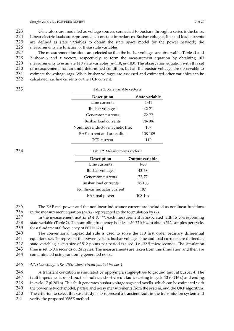
SNR of 0.001 pu or 0.1% is assumed for the noise process. Figure 3 shows the busbar voltages 1-30, 253

where the actual, the proposed UKF estimate and the difference between instantaneous values during 254

the fault at busbar 4 are shown, corresponding to state variables 42-71. 255

The largest estimation error is present when the fault condition is removed at 0.283 s; this error 256

is due to sudden changes in the busbar voltages. It is approximately 7%, but quickly decreases in the 257

next three cycles to 1%. These voltage fluctuations are due to the short-circuit transient condition at 258

busbar 4. 259

260

Figure 3. Busbar voltages (a) Actual, (b) UKF VSSE, (c) Difference, short-circuit at busbar 4 from 0.216 261

to 0.283 s. 262

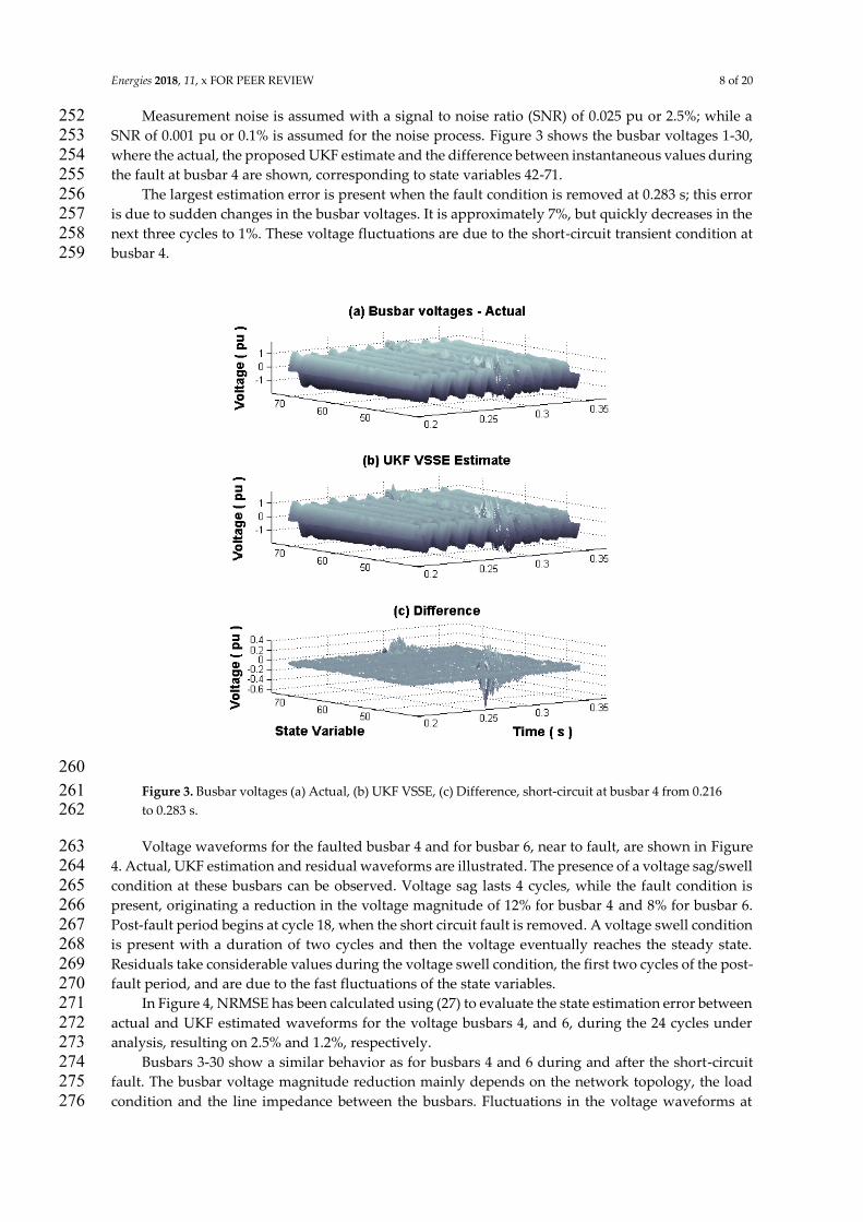
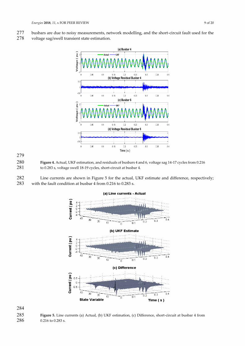
Voltage waveforms for the faulted busbar 4 and for busbar 6, near to fault, are shown in Figure 263

4. Actual, UKF estimation and residual waveforms are illustrated. The presence of a voltage sag/swell 264

condition at these busbars can be observed. Voltage sag lasts 4 cycles, while the fault condition is 265

present, originating a reduction in the voltage magnitude of 12% for busbar 4 and 8% for busbar 6. 266

Post-fault period begins at cycle 18, when the short circuit fault is removed. A voltage swell condition 267

is present with a duration of two cycles and then the voltage eventually reaches the steady state. 268

Residuals take considerable values during the voltage swell condition, the first two cycles of the post-269

fault period, and are due to the fast fluctuations of the state variables. 270

In Figure 4, NRMSE has been calculated using (27) to evaluate the state estimation error between 271

actual and UKF estimated waveforms for the voltage busbars 4, and 6, during the 24 cycles under 272

analysis, resulting on 2.5% and 1.2%, respectively. 273

Busbars 3-30 show a similar behavior as for busbars 4 and 6 during and after the short-circuit 274

fault. The busbar voltage magnitude reduction mainly depends on the network topology, the load 275

condition and the line impedance between the busbars. Fluctuations in the voltage waveforms at 276

Energies 2018, 11, x FOR PEER REVIEW 9 of 20

busbars are due to noisy measurements, network modelling, and the short-circuit fault used for the 277

voltage sag/swell transient state estimation. 278

279

Figure 4. Actual, UKF estimation, and residuals of busbars 4 and 6, voltage sag 14-17 cycles from 0.216 280

to 0.283 s, voltage swell 18-19 cycles, short-circuit at busbar 4. 281

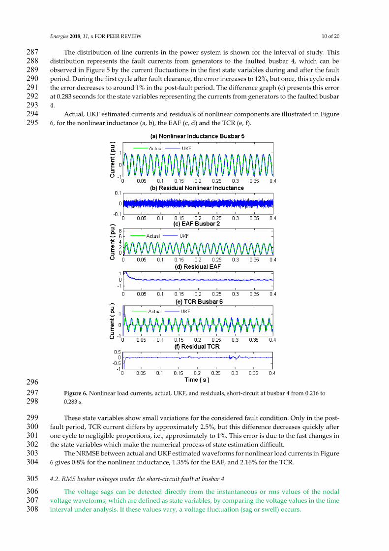
Line currents are shown in Figure 5 for the actual, UKF estimate and difference, respectively; 282

with the fault condition at busbar 4 from 0.216 to 0.283 s. 283

284

Figure 5. Line currents (a) Actual, (b) UKF estimation, (c) Difference, short-circuit at busbar 4 from 285

0.216 to 0.283 s. 286

Energies 2018, 11, x FOR PEER REVIEW 10 of 20

The distribution of line currents in the power system is shown for the interval of study. This 287

distribution represents the fault currents from generators to the faulted busbar 4, which can be 288

observed in Figure 5 by the current fluctuations in the first state variables during and after the fault 289

period. During the first cycle after fault clearance, the error increases to 12%, but once, this cycle ends 290

the error decreases to around 1% in the post-fault period. The difference graph (c) presents this error 291

at 0.283 seconds for the state variables representing the currents from generators to the faulted busbar 292

4. 293

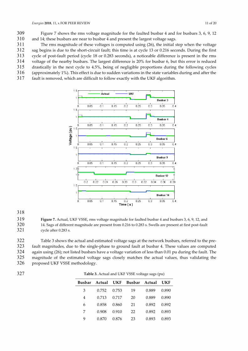
Actual, UKF estimated currents and residuals of nonlinear components are illustrated in Figure 294

6, for the nonlinear inductance (a, b), the EAF (c, d) and the TCR (e, f). 295

296

Figure 6. Nonlinear load currents, actual, UKF, and residuals, short-circuit at busbar 4 from 0.216 to 297

0.283 s. 298

These state variables show small variations for the considered fault condition. Only in the post-299

fault period, TCR current differs by approximately 2.5%, but this difference decreases quickly after 300

one cycle to negligible proportions, i.e., approximately to 1%. This error is due to the fast changes in 301

the state variables which make the numerical process of state estimation difficult. 302

The NRMSE between actual and UKF estimated waveforms for nonlinear load currents in Figure 303

6 gives 0.8% for the nonlinear inductance, 1.35% for the EAF, and 2.16% for the TCR. 304

4.2. RMS busbar voltages under the short-circuit fault at busbar 4 305

The voltage sags can be detected directly from the instantaneous or rms values of the nodal 306

voltage waveforms, which are defined as state variables, by comparing the voltage values in the time 307

interval under analysis. If these values vary, a voltage fluctuation (sag or swell) occurs. 308

Energies 2018, 11, x FOR PEER REVIEW 11 of 20

Figure 7 shows the rms voltage magnitude for the faulted busbar 4 and for busbars 3, 6, 9, 12 309

and 14; these busbars are near to busbar 4 and present the largest voltage sags. 310

The rms magnitude of these voltages is computed using (26), the initial step when the voltage 311

sag begins is due to the short-circuit fault; this time is at cycle 13 or 0.216 seconds. During the first 312

cycle of post-fault period (cycle 18 or 0.283 seconds), a noticeable difference is present in the rms 313

voltage of the nearby busbars. The largest difference is 20% for busbar 6, but this error is reduced 314

drastically in the next cycle to 4.5%, being of negligible proportions during the following cycles 315

(approximately 1%). This effect is due to sudden variations in the state variables during and after the 316

fault is removed, which are difficult to follow exactly with the UKF algorithm. 317

318

Figure 7. Actual, UKF VSSE, rms voltage magnitude for faulted busbar 4 and busbars 3, 6, 9, 12, and 319

14. Sags of different magnitude are present from 0.216 to 0.283 s. Swells are present at first post-fault 320

cycle after 0.283 s. 321

Table 3 shows the actual and estimated voltage sags at the network busbars, referred to the pre-322

fault magnitudes, due to the single-phase to ground fault at busbar 4. These values are computed 323

again using (26); not listed busbars have a voltage variation of less than 0.01 pu during the fault. The 324

magnitude of the estimated voltage sags closely matches the actual values, thus validating the 325

proposed UKF VSSE methodology. 326

Table 3. Actual and UKF VSSE voltage sags (pu) 327

Busbar Actual UKF Busbar Actual UKF

3 0.752 0.753 19 0.889 0.890

4 0.713 0.717 20 0.889 0.890

6 0.858 0.860 21 0.892 0.892

7 0.908 0.910 22 0.892 0.893

9 0.870 0.876 23 0.893 0.893

Energies 2018, 11, x FOR PEER REVIEW 12 of 20

10 0.890 0.900 24 0.887 0.888

12 0.870 0.880 25 0.888 0.889

14 0.880 0.885 26 0.892 0.892

15 0.872 0.873 27 0.891 0.892

16 0.880 0.890 28 0.880 0.881

17 0.892 0.895 29 0.884 0.885

18 0.875 0.880 30 0.907 0.909

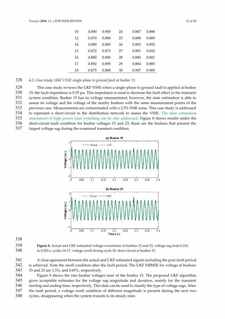
4.3. Case study: UKF VSSE single-phase to ground fault at busbar 15 328

This case study reviews the UKF VSSE when a single-phase to ground fault is applied at busbar 329

15; the fault impedance is 0.35 pu. This impedance is used to decrease the fault effect in the transient 330

system condition. Busbar 15 has no voltage measurement, however, the state estimation is able to 331

assess its voltage and the voltage of the nearby busbars with the same measurement points of the 332

previous case. Measurements are contaminated with a 2.5% SNR noise. This case study is addressed 333

to represent a short-circuit in the distribution network to assess the VSSE. The state estimation 334

assessment of high power load switching can be also addressed. Figure 8 shows results under the 335

short-circuit fault condition for busbar voltages 15 and 23; these are the busbars that present the 336

largest voltage sag during the examined transient condition. 337

338

Figure 8. Actual and UKF estimated voltage waveforms of busbars 15 and 23, voltage sag from 0.216 339

to 0.283 s, cycles 14-17, voltage swell during cycle 18, short-circuit at busbar 15. 340

A close agreement between the actual and UKF estimated signals including the post-fault period 341

is achieved. Note the swell condition after the fault period. The UKF NRMSE for voltage at busbars 342

15 and 23 are 1.5%, and 0.65%, respectively. 343

Figure 9 shows the rms busbar voltages near of the busbar 15. The proposed UKF algorithm 344

gives acceptable estimates for the voltage sag magnitude and duration, mainly for the transient 345

starting and ending time, respectively. This data can be used to classify the type of voltage sags. After 346

the fault period, a voltage swell condition of different magnitude is present during the next two 347

cycles, disappearing when the system transits to its steady state. 348

Energies 2018, 11, x FOR PEER REVIEW 13 of 20

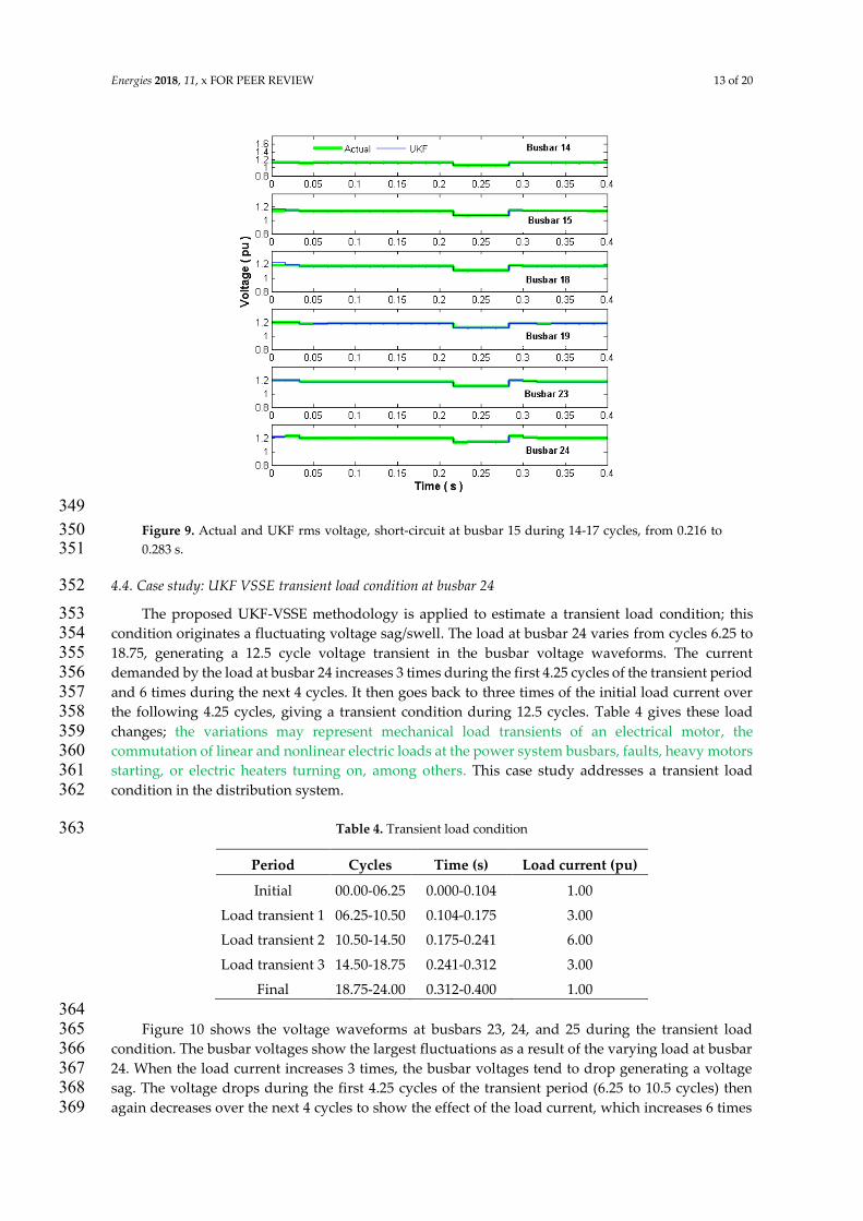
349

Figure 9. Actual and UKF rms voltage, short-circuit at busbar 15 during 14-17 cycles, from 0.216 to 350

0.283 s. 351

4.4. Case study: UKF VSSE transient load condition at busbar 24 352

The proposed UKF-VSSE methodology is applied to estimate a transient load condition; this 353

condition originates a fluctuating voltage sag/swell. The load at busbar 24 varies from cycles 6.25 to 354

18.75, generating a 12.5 cycle voltage transient in the busbar voltage waveforms. The current 355

demanded by the load at busbar 24 increases 3 times during the first 4.25 cycles of the transient period 356

and 6 times during the next 4 cycles. It then goes back to three times of the initial load current over 357

the following 4.25 cycles, giving a transient condition during 12.5 cycles. Table 4 gives these load 358

changes; the variations may represent mechanical load transients of an electrical motor, the 359

commutation of linear and nonlinear electric loads at the power system busbars, faults, heavy motors 360

starting, or electric heaters turning on, among others. This case study addresses a transient load 361

condition in the distribution system. 362

Table 4. Transient load condition 363

Period Cycles Time (s) Load current (pu)

Initial 00.00-06.25 0.000-0.104 1.00

Load transient 1 06.25-10.50 0.104-0.175 3.00

Load transient 2 10.50-14.50 0.175-0.241 6.00

Load transient 3 14.50-18.75 0.241-0.312 3.00

Final 18.75-24.00 0.312-0.400 1.00

364

Figure 10 shows the voltage waveforms at busbars 23, 24, and 25 during the transient load 365

condition. The busbar voltages show the largest fluctuations as a result of the varying load at busbar 366

24. When the load current increases 3 times, the busbar voltages tend to drop generating a voltage 367

sag. The voltage drops during the first 4.25 cycles of the transient period (6.25 to 10.5 cycles) then 368

again decreases over the next 4 cycles to show the effect of the load current, which increases 6 times 369

Energies 2018, 11, x FOR PEER REVIEW 14 of 20

during those 4 cycles (10.5 to 14.5 cycles). Finally, the current goes back to three times of the value at 370

the initial period (14.5 to 18.75 cycles). 371

Load transient initiates at 6.25 cycles instead of 6 cycles to evaluate a more critical transient; 372

similarly, the load transient finishes at 18.75 cycles instead of 18 cycles. 373

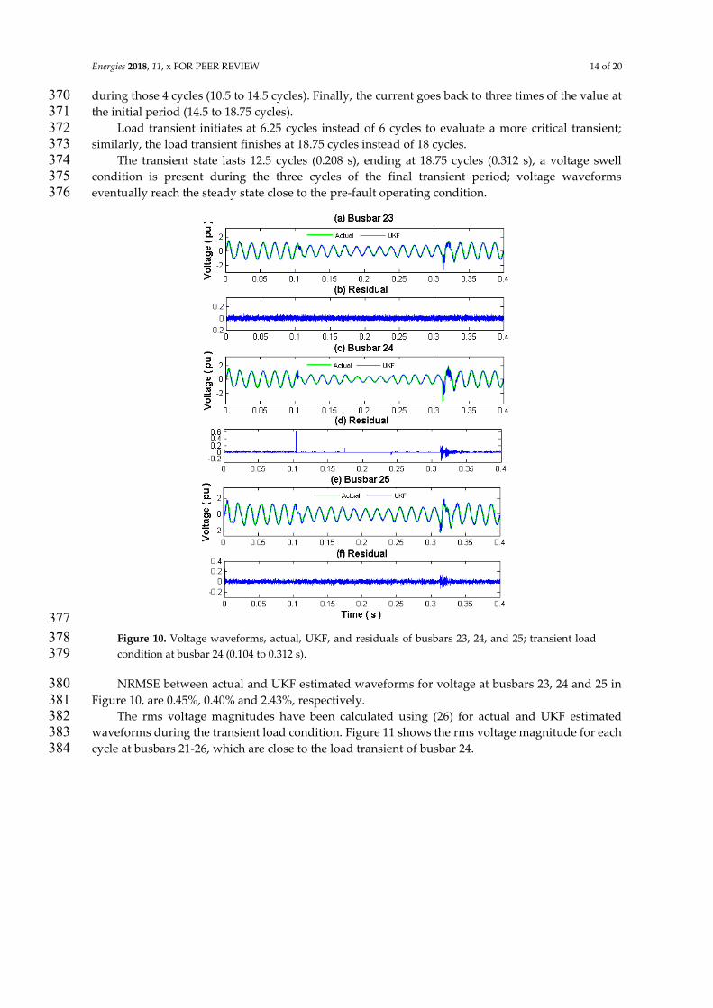
The transient state lasts 12.5 cycles (0.208 s), ending at 18.75 cycles (0.312 s), a voltage swell 374

condition is present during the three cycles of the final transient period; voltage waveforms 375

eventually reach the steady state close to the pre-fault operating condition. 376

377

Figure 10. Voltage waveforms, actual, UKF, and residuals of busbars 23, 24, and 25; transient load 378

condition at busbar 24 (0.104 to 0.312 s). 379

NRMSE between actual and UKF estimated waveforms for voltage at busbars 23, 24 and 25 in 380

Figure 10, are 0.45%, 0.40% and 2.43%, respectively. 381

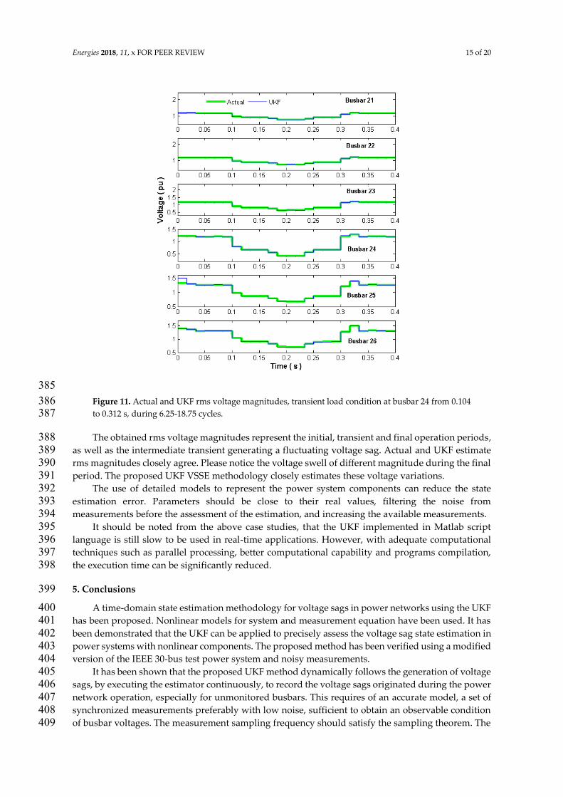
The rms voltage magnitudes have been calculated using (26) for actual and UKF estimated 382

waveforms during the transient load condition. Figure 11 shows the rms voltage magnitude for each 383

cycle at busbars 21-26, which are close to the load transient of busbar 24. 384

Energies 2018, 11, x FOR PEER REVIEW 15 of 20

385

Figure 11. Actual and UKF rms voltage magnitudes, transient load condition at busbar 24 from 0.104 386

to 0.312 s, during 6.25-18.75 cycles. 387

The obtained rms voltage magnitudes represent the initial, transient and final operation periods, 388

as well as the intermediate transient generating a fluctuating voltage sag. Actual and UKF estimate 389

rms magnitudes closely agree. Please notice the voltage swell of different magnitude during the final 390

period. The proposed UKF VSSE methodology closely estimates these voltage variations. 391

The use of detailed models to represent the power system components can reduce the state 392

estimation error. Parameters should be close to their real values, filtering the noise from 393

measurements before the assessment of the estimation, and increasing the available measurements. 394

It should be noted from the above case studies, that the UKF implemented in Matlab script 395

language is still slow to be used in real-time applications. However, with adequate computational 396

techniques such as parallel processing, better computational capability and programs compilation, 397

the execution time can be significantly reduced. 398

5. Conclusions 399

A time-domain state estimation methodology for voltage sags in power networks using the UKF 400

has been proposed. Nonlinear models for system and measurement equation have been used. It has 401

been demonstrated that the UKF can be applied to precisely assess the voltage sag state estimation in 402

power systems with nonlinear components. The proposed method has been verified using a modified 403

version of the IEEE 30-bus test power system and noisy measurements. 404

It has been shown that the proposed UKF method dynamically follows the generation of voltage 405

sags, by executing the estimator continuously, to record the voltage sags originated during the power 406

network operation, especially for unmonitored busbars. This requires of an accurate model, a set of 407

synchronized measurements preferably with low noise, sufficient to obtain an observable condition 408

of busbar voltages. The measurement sampling frequency should satisfy the sampling theorem. The 409

Energies 2018, 11, x FOR PEER REVIEW 16 of 20

rms value can be computed from discrete waveforms; this value gives the information to define the 410

sag magnitude, delimiting the sag time interval. 411

From the conducted case studies, it has been observed that when the power system goes under 412

fast transients, the UKF estimator error is more noticeable; however, as the network evolves to steady 413

state, the error quickly decreases to negligible proportions, i.e. on average 1%. In most cases, this 414

period is short compared with the voltage sag estimation interval. This condition is present during 415

the final period of the reviewed case studies, when the fault or transient condition is removed. It 416

should be noted that usually at this time, a voltage swell is generated. 417

The state estimation error increases when sudden transient variations are present. The results 418

obtained with the proposed UKF VSSE methodology have been successfully compared against actual 419

values taken from a simulation of the test power system under the same transient condition. A close 420

agreement has been achieved in all cases between the compared responses. 421

Acknowledgements: The authors gratefully acknowledge the Universidad Michoacana de San 422

Nicolás de Hidalgo through the Facultad de Ingeniería Eléctrica, División de Estudios de Posgrado 423

(FIE-DEP) Morelia, México, for the facilities granted to carry out this investigation. First two authors 424

acknowledge financial assistance from CONACYT to conduct this investigation. 425

Author Contributions: Rafael Cisneros-Magaña performed the simulation and modelling, analyzed 426

the data, and wrote the paper. Aurelio Medina analyzed the results, reviewed the modeling and text, 427

and supervised the related research work. Olimpo Anaya-Lara provided critical comments and 428

revised the paper. 429

Conflicts of Interest: The authors declare no conflict of interest. 430

Nomenclature 431

List of Abbreviations 432

EAF Electric arc furnace 433

FACTS Flexible alternating current transmission system 434

KF Kalman filter 435

NRMSE Normalized root mean square error 436

PQ Power quality 437

SNR Signal to noise ratio 438

STATCOM Static synchronous compensator 439

TCR Thyristor-controlled rectifier 440

UKF Unscented Kalman filter 441

UT Unscented transform 442

VSSE Voltage sags state estimation 443

WAMS Wide area measurement system 444

List of Symbols 445

e State estimation error vector 446

f Nonlinear state function 447

h Nonlinear output function 448

k Time instant t=k┡t 449

k+1 Time instant t=(k+ｱ《┡t 450

m Number of measurements 451

n Number of state variables 452

t Time vector 453

u Input vector 454

v Process noise vector 455

w Measurement noise vector 456

x State vector 457 姉赴 Estimated state vector 458

y Output vector 459

Energies 2018, 11, x FOR PEER REVIEW 17 of 20

z Measurement vector 460

E Expected value 461

H Measurements matrix 462

K Kalman filter gain matrix 463

N Normal distribution 464

P Error covariance matrix 465

Q Process noise covariance matrix 466

R Measurement noise covariance matrix 467

Vrms Rms voltage magnitude 468

W Scalar weights 469

+ A posteriori or after measurement estimate 470

む A priori or before measurement estimate 471

┡t Step time 472

ぼ Parameter to determine the spread of sigma points 473

ぽ Parameter to determine the distribution of x 474

ゆ Scaling parameter 475

ま Scaling parameter 476

ゅ Parameter to determine the spread of sigma points 477 璽 Sigma points matrix 478

Appendix A Per unit additional nonlinear load parameters 479

EAF busbar 2: Leaf=0.5, k1=0.004, k2=0.0005, k3=0.005, m=0, n=2.0, initial condition EAF arc 480

radius=0.1 481

Nonlinear inductance busbar 5: Rm=4.0, Lm=1.0, n=5.0, a=0, b=0.3 482

TCR busbar 6: Rtcr=1.0, Ltcr=0.5, firing angle ぼ=100 deg. 483

Appendix B Nonlinear models 484

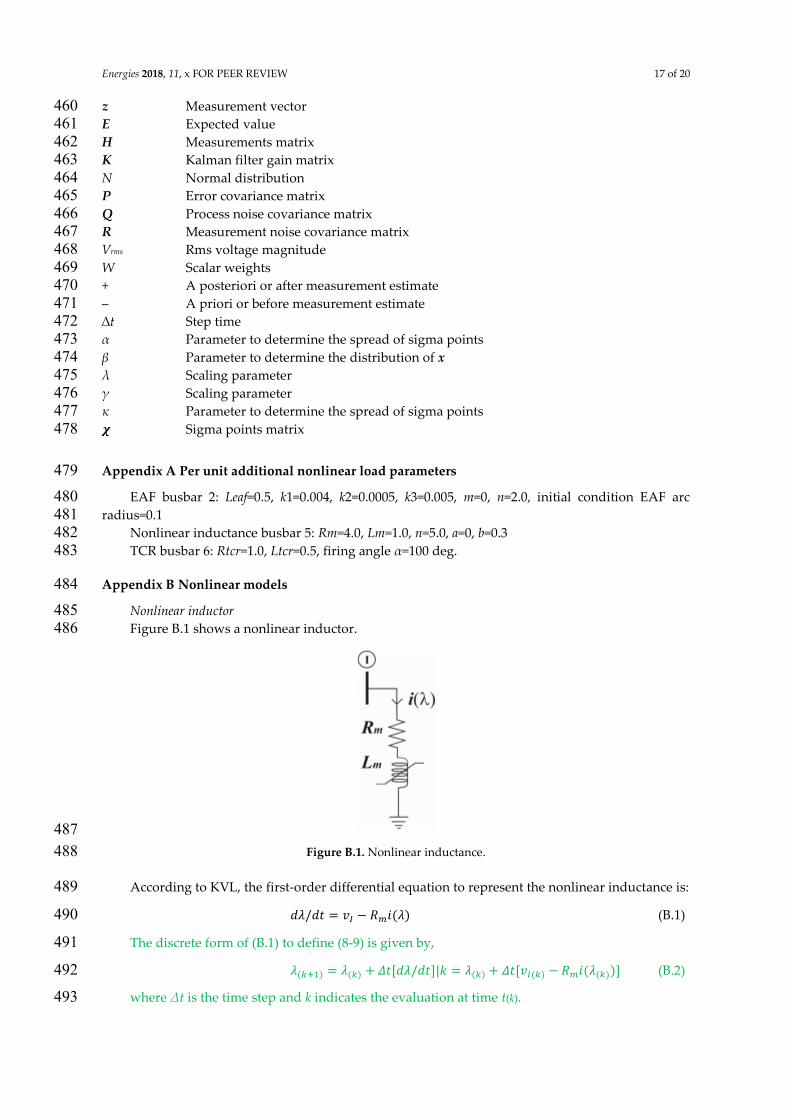
Nonlinear inductor 485

Figure B.1 shows a nonlinear inductor. 486

487

Figure B.1. Nonlinear inductance. 488

According to KVL, the first-order differential equation to represent the nonlinear inductance is: 489 穴膏【穴建 噺 懸彫 伐 迎陳件岫膏岻 (B.1) 490

The discrete form of (B.1) to define (8-9) is given by, 491 膏岫賃袋怠岻 噺 膏岫賃岻 髪 弘建岷穴膏【穴建峅】倦 噺 膏岫賃岻 髪 弘建岷懸彫岫賃岻 伐 迎陳件岫膏岫賃岻岻峅 (B.2) 492

where ♪t is the time step and k indicates the evaluation at time t(k). 493

Energies 2018, 11, x FOR PEER REVIEW 18 of 20

The nonlinear solution of (B.1), is represented by i(ゆ), ゆ is the nonlinear inductor magnetic flux, 494

the polynomial approximation for i(ゆ) is, 495 件岫膏岻 噺 欠膏 髪 決膏津 (B.3) 496

n is an odd number due to the odd symmetry of (B.3). Coefficients a, b and n adjust the nonlinear 497

saturation curve. The rational fractions and hyperbolic approximations are alternative methods to 498

represent this nonlinearity [38-39]. 499

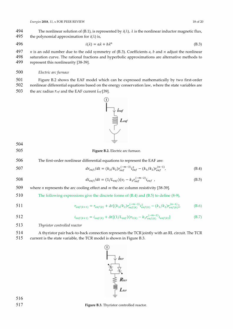
Electric arc furnace 500

Figure B.2 shows the EAF model which can be expressed mathematically by two first-order 501

nonlinear differential equations based on the energy conservation law, where the state variables are 502

the arc radius reaf and the EAF current ieaf [39]. 503

504

Figure B.2. Electric arc furnace. 505

The first-order nonlinear differential equations to represent the EAF are: 506 穴堅勅銚捗【穴建 噺 岫倦戴【倦態岻堅勅銚捗岫貸陳貸戴岻件勅銚捗態 伐 岫倦怠【倦態岻堅勅銚捗岫津貸怠岻, (B.4) 507

穴件勅銚捗【穴建 噺 岫な【詣勅銚捗岻岫懸彫 伐 倦戴堅勅銚捗岫貸陳貸態岻件勅銚捗 , (B.5) 508

where n represents the arc cooling effect and m the arc column resistivity [38-39]. 509

The following expressions give the discrete forms of (B.4) and (B.5) to define (8-9), 510 堅勅銚捗岫賃袋怠岻 噺 堅勅銚捗岫賃岻 髪 弘建岷岫倦戴【倦態岻堅勅銚捗岫賃岻岫貸陳貸戴岻件勅銚捗岫賃岻態 伐 岫倦怠【倦態岻堅勅銚捗岫賃岻岫津貸怠岻 峅, (B.6) 511

件勅銚捗岫賃袋怠岻 噺 件勅銚捗岫賃岻 髪 弘建岷岫な【詣勅銚捗岻岫懸彫岫賃岻 伐 倦戴堅勅銚捗岫賃岻岫貸陳貸態岻件勅銚捗岫賃岻] (B.7) 512

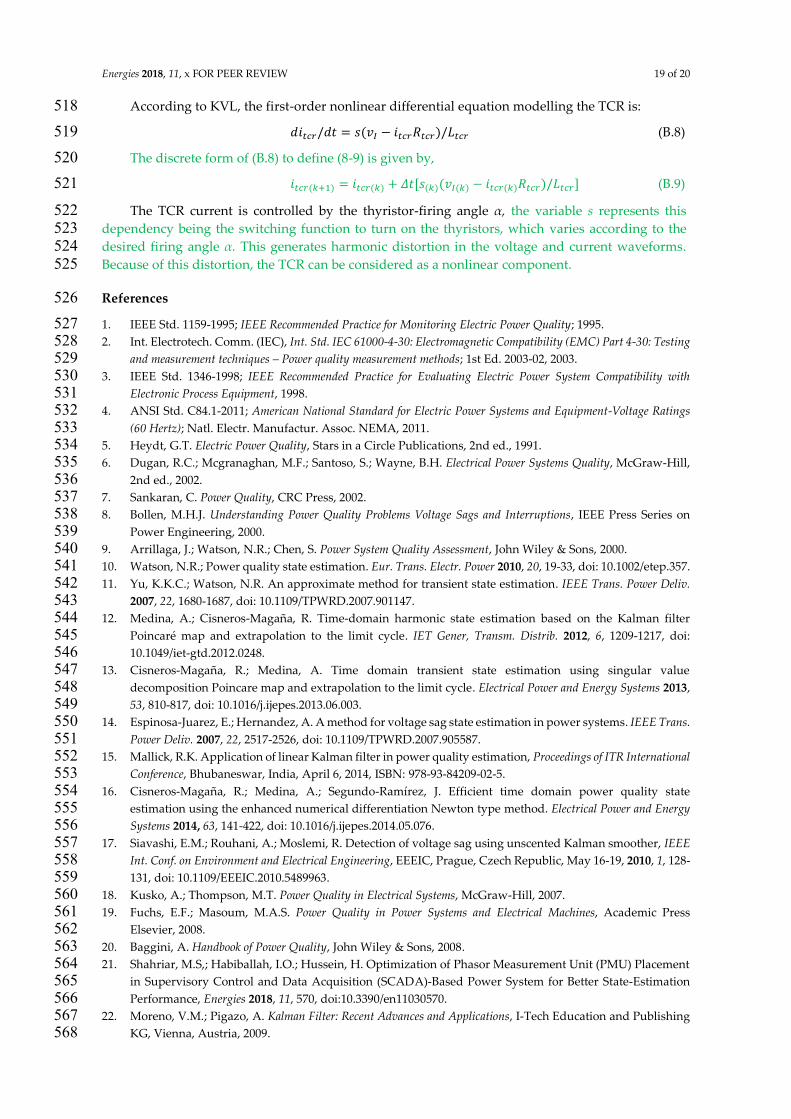
Thyristor controlled reactor 513

A thyristor pair back-to-back connection represents the TCR jointly with an RL circuit. The TCR 514

current is the state variable, the TCR model is shown in Figure B.3. 515

516

Figure B.3. Thyristor controlled reactor. 517

Energies 2018, 11, x FOR PEER REVIEW 19 of 20

According to KVL, the first-order nonlinear differential equation modelling the TCR is: 518 穴件痛頂追【穴建 噺 嫌岫懸彫 伐 件痛頂追迎痛頂追岻【詣痛頂追 (B.8) 519

The discrete form of (B.8) to define (8-9) is given by, 520 件痛頂追岫賃袋怠岻 噺 件痛頂追岫賃岻 髪 弘建岷嫌岫賃岻岫懸彫岫賃岻 伐 件痛頂追岫賃岻迎痛頂追岻【詣痛頂追峅 (B.9) 521

The TCR current is controlled by the thyristor-firing angle ぼ╇ the variable s represents this 522

dependency being the switching function to turn on the thyristors, which varies according to the 523

desired firing angle ぼ. This generates harmonic distortion in the voltage and current waveforms. 524

Because of this distortion, the TCR can be considered as a nonlinear component. 525

References 526

1. IEEE Std. 1159-1995; IEEE Recommended Practice for Monitoring Electric Power Quality; 1995. 527

2. Int. Electrotech. Comm. (IEC), Int. Std. IEC 61000-4-30: Electromagnetic Compatibility (EMC) Part 4-30: Testing 528

and measurement techniques む Power quality measurement methods; 1st Ed. 2003-02, 2003. 529

3. IEEE Std. 1346-1998; IEEE Recommended Practice for Evaluating Electric Power System Compatibility with 530

Electronic Process Equipment, 1998. 531

4. ANSI Std. C84.1-2011; American National Standard for Electric Power Systems and Equipment-Voltage Ratings 532

(60 Hertz); Natl. Electr. Manufactur. Assoc. NEMA, 2011. 533

5. Heydt, G.T. Electric Power Quality, Stars in a Circle Publications, 2nd ed., 1991. 534

6. Dugan, R.C.; Mcgranaghan, M.F.; Santoso, S.; Wayne, B.H. Electrical Power Systems Quality, McGraw-Hill, 535

2nd ed., 2002. 536

7. Sankaran, C. Power Quality, CRC Press, 2002. 537

8. Bollen, M.H.J. Understanding Power Quality Problems Voltage Sags and Interruptions, IEEE Press Series on 538

Power Engineering, 2000. 539

9. Arrillaga, J.; Watson, N.R.; Chen, S. Power System Quality Assessment, John Wiley & Sons, 2000. 540

10. Watson, N.R.; Power quality state estimation. Eur. Trans. Electr. Power 2010, 20, 19-33, doi: 10.1002/etep.357. 541

11. Yu, K.K.C.; Watson, N.R. An approximate method for transient state estimation. IEEE Trans. Power Deliv. 542

2007, 22, 1680-1687, doi: 10.1109/TPWRD.2007.901147. 543

12. Medina, A.; Cisneros-Magaña, R. Time-domain harmonic state estimation based on the Kalman filter 544

Poincaré map and extrapolation to the limit cycle. IET Gener, Transm. Distrib. 2012, 6, 1209-1217, doi: 545

10.1049/iet-gtd.2012.0248. 546

13. Cisneros-Magaña, R.; Medina, A. Time domain transient state estimation using singular value 547

decomposition Poincare map and extrapolation to the limit cycle. Electrical Power and Energy Systems 2013, 548

53, 810-817, doi: 10.1016/j.ijepes.2013.06.003. 549

14. Espinosa-Juarez, E.; Hernandez, A. A method for voltage sag state estimation in power systems. IEEE Trans. 550

Power Deliv. 2007, 22, 2517-2526, doi: 10.1109/TPWRD.2007.905587. 551

15. Mallick, R.K. Application of linear Kalman filter in power quality estimation, Proceedings of ITR International 552

Conference, Bhubaneswar, India, April 6, 2014, ISBN: 978-93-84209-02-5. 553

16. Cisneros-Magaña, R.; Medina, A.; Segundo-Ramírez, J. Efficient time domain power quality state 554

estimation using the enhanced numerical differentiation Newton type method. Electrical Power and Energy 555

Systems 2014, 63, 141-422, doi: 10.1016/j.ijepes.2014.05.076. 556

17. Siavashi, E.M.; Rouhani, A.; Moslemi, R. Detection of voltage sag using unscented Kalman smoother, IEEE 557

Int. Conf. on Environment and Electrical Engineering, EEEIC, Prague, Czech Republic, May 16-19, 2010, 1, 128-558

131, doi: 10.1109/EEEIC.2010.5489963. 559

18. Kusko, A.; Thompson, M.T. Power Quality in Electrical Systems, McGraw-Hill, 2007. 560

19. Fuchs, E.F.; Masoum, M.A.S. Power Quality in Power Systems and Electrical Machines, Academic Press 561

Elsevier, 2008. 562

20. Baggini, A. Handbook of Power Quality, John Wiley & Sons, 2008. 563

21. Shahriar, M.S,; Habiballah, I.O.; Hussein, H. Optimization of Phasor Measurement Unit (PMU) Placement 564

in Supervisory Control and Data Acquisition (SCADA)-Based Power System for Better State-Estimation 565

Performance, Energies 2018, 11, 570, doi:10.3390/en11030570. 566

22. Moreno, V.M.; Pigazo, A. Kalman Filter: Recent Advances and Applications, I-Tech Education and Publishing 567

KG, Vienna, Austria, 2009. 568

Energies 2018, 11, x FOR PEER REVIEW 20 of 20

23. Chen, R.; Lin, T.; Bi, R.; Xu, X. Novel Strategy for Accurate Locating of Voltage Sag Sources in Smart 569

Distribution Networks with Inverter-Interfaced Distributed Generators, Energies 2017, 10, 1885, 570

doi:10.3390/en10111885. 571

24. Amit, J.; Shivakumar, N.R. Power system tracking and dynamic state estimation, Power Systems Conf. & 572

Exp., PSCE, Seattle, WA, USA, Mar. 15-18, 2009, doi: 10.1109/PSCE.2009.4840192. 573

25. Wang, S.; Gao, W.; Meliopoulos, A.P.S. An alternative method for power system dynamic state estimation 574

based on unscented transform, IEEE Trans. Power Syst. 2012, 27, 942-950, doi: 10.1109/TPWRS.2011.2175255. 575

26. Charalampidis, A.C.; Papavassilopoulos, G.P. Development and numerical investigation of new non-576

linear Kalman filter variants, IET Control Theory & Appl. 2011, 5, 1155-1166, doi: 10.1049/iet-cta.2010.0553. 577

27. Tebianian, H.; Jeyasurya, B. Dynamic state estimation in power systems: Modeling, and challenges, Electr. 578

Power Syst. Res. 2015, 121, 109-114, doi: 10.1016/j.epsr.2014.12.005. 579

28. Lalami, A.; Wamkeue, R.; Kamwa, I.; Saad, M.; Beaudoin, J.J. Unscented Kalman filter for non-linear 580

estimation of induction machine parameters, IET Electr. Power Appl. 2012, 6, 611-620, doi: 10.1049/iet-581

epa.2012.0026. 582

29. Ghahremani, E.; Kamwa, I. Online state estimation of a synchronous generator using unscented Kalman 583

filter from phasor measurements units, IEEE Trans. Energy Convers. 2011, 26, 1099-1108, doi: 584

10.1109/TEC.2011.2168225. 585

30. Julier, S.J.; Uhlmann, J.K. Unscented filtering and nonlinear estimation, Proc. IEEE 2004, 92, 401-422, doi: 586

10.1109/JPROC.2003.823141. 587

31. Qing, X.; Yang, F.; Wang, X. Extended set-membership filter for power system dynamic state estimation, 588

Electr. Power Syst. Res. 2013, 99, 56-63, doi: 10.1016/j.epsr.2013.02.002. 589

32. Huang, M.; Li, W.; Yan, W. Estimating parameters of synchronous generators using square-root unscented 590

Kalman filter, Electr. Power Syst. Res. 2010, 80, 1137-1144, doi: 10.1016/j.epsr.2010.03.007. 591

33. Van der Merwe, R.; Wan, E.A. The square-root unscented Kalman filter for state and parameter estimation, 592

IEEE Int. Conf. on Acoustics, Speech, and Signal Processing, ICASSP, Salt Lake City, UT, USA, May 7-11, 593

2001, 6, 3461-3464. 594

34. Aghamolki, H.G.; Miao, Z.; Fan, L.; Jiang, W.; Manjure, D. Identification of synchronous generator model 595

with frequency control using unscented Kalman filter, Electr. Power Syst. Res. 2015, 126, 45-55, doi: 596

10.1016/j.epsr.2015.04.016. 597

35. Bretas, N.; Bretas, A.; Piereti, S. Innovation concept for measurement gross error detection and 598

identification in power system state estimation, IET Gener., Transm. & Distrib. 2011, 5, 603-608, doi: 599

10.1049/iet-gtd.2010.0459. 600

36. Jain, S.K.; Singh, S.N. Harmonics estimation in emerging power system: Key issues and challenges, Electr. 601

Power Syst. Res. 2011, 81, 1754-1766, doi: 10.1016/j.epsr.2011.05.004. 602

37. University of Washington, Electrical Engineering, Power Systems Test Case Archive. 603

http://www.ee.washington.edu/research/pstca/pf30/pg_tca30bus.htm, (accessed on 15 03 18). 604

38. Task Force on Harmonics Modeling and Simulation, Modeling devices with nonlinear voltage-current 605

characteristics for harmonic studies, IEEE Trans. Power Deliv. 2004, 19, 1802-1811, doi: 606

10.1109/TPWRD.2004.835429. 607

39. Acha, E.; Madrigal, M. Power Systems Harmonics Computer Modelling and Analysis, John Wiley & Sons, 2001. 608

© 2018 by the authors. Submitted for possible open access publication under the 609

terms and conditions of the Creative Commons Attribution (CC BY) license 610

(http://creativecommons.org/licenses/by/4.0/). 611