Cities as complex systems: scaling, interactions, networks, dynamics and urban morphologies

UCL CENTRE FOR ADVANCED SPATIAL ANALYSIS

Centre for Advanced Spatial Analysis University College London 1 - 19 Torrington Place Gower St London WC1E 7HBTel: +44 (0)20 7679 1782 [email protected] www.casa.ucl.ac.uk

WORKINGPAPERSSERIESCities as Complex Systems: Scaling, Interactions, Networks, Dynamicsand Urban Morphologies

ISSN 1467-1298

Paper 131 - Feb 08

1

Cities as Complex Systems†

Scaling, Interactions, Networks, Dynamics and Urban Morphologies

Michael Batty

Centre for Advanced Spatial Analysis, University College London, 1-19 Torrington Place, London WC1E 6BT, UK

Email: [email protected], Web: www.casa.ucl.ac.uk

Abstract

Cities have been treated as systems for fifty year but only in the last two decades has the focus changed from aggregate equilibrium systems to more evolving systems whose structure merges from the bottom up. We first outline the rudiments of the traditional approach focusing on equilibrium and then discuss how the paradigm has changed to one which treats cities as emergent phenomena generated through a combination of hierarchical levels of decision, driven in decentralized fashion. This is consistent with the complexity sciences which dominate the simulation of urban form and function. We begin however with a review of equilibrium models, particularly those based on spatial interaction, and we then explore how simple dynamic frameworks can be fashioned to generate more realistic models. In exploring dynamics, nonlinear systems which admit chaos and bifurcation have relevance but recently more pragmatic schemes of structuring urban models based on cellular automata and agent-based modeling principles have come to the fore. Most urban models deal with the city in terms of the location of its economic and demographic activities but there is also a move to link such models to urban morphologies which are clearly fractal in structure. Throughout this chapter, we show how key concepts in complexity such as scaling, self-similarity and far-from-equilibrium structures dominate our current treatment of cities, how we might simulate their functioning and how we might predict their futures. We conclude with the key problems that dominate the field and suggest how these might be tackled in future research.

†in The Encyclopedia of Complexity & System Science, Springer, Berlin, DE, forthcoming 2008. Date of this paper: February 25, 2008.

2

Glossary

Agent-Based Models: systems composed of individuals who act

purposely in making locational/spatial decisions Bifurcation: a process whereby divergent paths are generated in a

trajectory of change in an urban system City Size Distribution: a set of cities by size, usually population,

often in rank order Emergent Patterns: land uses or economic activities which follow

some spatial order Entropy Maximizing: the process of generating a spatial model by

maximizing a measure of system complexity subject to constraints Equilibrium: a state of the urban system which is balanced and

unchanging Exponential Growth: the process whereby an activity changes

through positive feedback on itself Fast Dynamics: a process of frequent movement between locations,

often daily Feedback: the process whereby a system variable influences another

variable, either positively or negatively Fractal Structure: a pattern or arrangement of system elements that

are self-similar at different spatial scales Land Use Transport Model: a model linking urban activities to

transport interactions Life Cycle Effects: changes in spatial location which are motivated by

aging of urban activities and populations Local Neighborhood: the space immediately around a zone or cell Logistic Growth: exponential growth capacitated so that some density

limit is not exceeded Lognormal Distribution: a distribution which has fat and long tails

which is normal when examined on a logarithmic scale Microsimulation: the process of generating synthetic populations

from data which is collated from several sources Model Validation: the process of calibrating and testing a model

against data so that its goodness of fit is optimized Multipliers: relationships which embody n’th order effects of one

variable on another. Network Scaling: the in-degrees and out-degrees of a graph whose

nodal link volumes follow a power law Population Density Profile: a distribution of populations which

typically follows an exponential profile when arrayed against distance from some nodal point

Power Laws: scaling laws that order a set of objects according to their size raised to some power

Rank Size Rule: a power law that rank orders a set of objects Reaction-Diffusion: the process of generating changes as a

consequence of a reaction to an existing state and interactions between states

3

Scale-free Networks: networks whose nodal volumes follow a power law

Segregation Model: a model which generates extreme global segregation from weak assumptions about local segregation

Simulation: the process of generating locational distributions according to a series of sub-model equations or rules

Slow Dynamics: changes in the urban system that take place over years or decades

Social Physics: the application of classical physical principles involving distance, force and mass to social situations, particularly to cities and their transport

Spatial Interaction: the movement of activities between different locations ranging from traffic distributions to migration patterns

Trip Distribution: the pattern of movement relating to trips made by the population, usually from home to work but also to other activities such as shopping

Urban Hierarchy: a set of entities physically or spatially scaled in terms of their size and areal extent

Urban Morphology: patterns of urban structure based on the way activities are ordered with respect to their locations

Urban System: a city represented as a set if interacting subsystems or their elements

4

Introduction: Cities as Systems

Cities were first treated formally as systems when General System Theory and

Cybernetics came to be applied to the softer social sciences in the 1950s. Ludwig von

Bertalanffy (1969) in biology and Norbert Weiner (1948) in engineering gave

enormous impetus to this emerging interdisciplinary field that thrust upon us the idea

that phenomena of interest in many disciplines could be articulated in generic terms as

‘systems’. Moreover the prospect that the systems approach could yield generic policy,

control and management procedures applicable to many different areas, appeared

enticing. The idea of a general systems theory was gradually fashioned from

reflections on the way distinct entities which were clearly collections of lower order

elements, organized into a coherent whole, displaying pattern and order which in the

jargon of the mid-twentieth century was encapsulated in the phrase that “the whole is

greater than the sum of the parts”. The movement began in biology in the 1920s,

gradually eclipsing parts of engineering in the 1950s and spreading to the

management and social sciences, particularly sociology and political science in the

1960s. It was part of a wave of change in the social sciences which began in the late

19th century as these fields began to emulate the physical sciences, espousing

positivist methods which had appeared so successful in building applicable and robust

theory.

The focus then was on ways in which the elements comprising the system interacted

with one another through structures that embodied feedbacks keeping the system

sustainable within bounded limits. The notion that such systems have controllers to

‘steer’ them to meet certain goals or targets is central to this early paradigm and the

science of “…control and communication in the animal and the machine” was the

definition taken up by Norbert Wiener (1948) in his exposition of the science of

cybernetics. General system theory provided the generic logic for both the structure

and behavior of such systems through various forms of feedback and hierarchical

organization while cybernetics represents the ‘science of steersmanship’ which would

enable such systems to move towards explicit goals or targets. Cities fit this

characterization admirably and in the 1950s and 1960s, the traditional approach that

articulated cities as structures that required physical and aesthetic organization,

5

quickly gave way to deeper notions that cities needed to be understood as general

systems. Their control and planning thus required much more subtle interventions

than anything that had occurred hitherto in the name of urban planning.

Developments in several disciplines supported these early developments. Spatial

analysis, as it is now called, began to develop within quantitative geography, linked to

the emerging field of regional science which represented a synthesis of urban and

regional economics in which location theory was central. In this sense, the economic

structure of cities and regions was consistent with classical macro and micro

economics and the various techniques and models that were developed within these

domains had immediate applicability. Applications of physical analogies to social and

city systems, particularly ideas about gravitation and potential, had been explored

since the mid 19th century under the banner of ‘social physics’ and as transportation

planning formally began in the 1950s, these ideas were quickly adopted as a basis for

transport modeling. Softer approaches in sociology and political science also provided

support for the idea of cities as organizational systems while the notion of cybernetics

as the basis for management, policy and control of cities was adopted as an important

analogy in their planning (Chadwick, 1971; McLoughlin, 1969).

The key ideas defined cities as sets of elements or components tied together through

sets of interactions. The archetypal structure was fashioned around land use activities

with economic and functional linkages between them represented initially in terms of

physical movement, traffic. The key idea of feedback, which is the dynamic that holds

a general system together, was largely represented in terms of the volume and pattern

of these interactions, at a single point in time. Longer term evolution of urban

structure was not central to these early conceptions for the focus was largely on how

cities functioned as equilibrium structures. The prime imperative was improving how

interactions between component land uses might be made more efficient while also

meeting goals involving social and spatial equity. Transportation and housing were of

central importance in adopting the argument that cities should be treated as examples

of general systems and steered according to the principles of cybernetics.

Typical examples of such systemic principles in action involve transportation in large

cities and these early ideas about systems theory hold as much sway in helping make

6

sense of current patterns as they did when they were first mooted fifty or more years

ago. Different types of land use with different economic foci interact spatially with

respect to how employees are linked to their housing locations, how goods are

shipped between different locations to service the production and consumption that

define these activities, how consumers purchase these economic activities which are

channeled through retail and commercial centers, how information flows tie all these

economies together, and so on: the list of linkages is endless. These activities are

capacitated by upper limits on density and capacity. In Greater London for example,

the traffic has reached saturation limits in the central city and with few new roads

being constructed over the last 40 years, the focus has shifted to improving public

transport and to road pricing.

The essence of using a systems model of spatial interaction to test the impact of such

changes on city structure is twofold: first such a model can show how people might

shift mode of transport from road to rail and bus, even to walking and cycling, if

differential pricing is applied to the road system. The congestion charge in central

London imposed in 2003 led to a 30 percent reduction in the use of vehicles and this

charge is set to increase massively for certain categories of polluting vehicles in the

near future. Second the slightly longer term effects of reducing traffic are to increase

densities of living, thus decreasing the length and cost of local work journeys, also

enabling land use to respond by changing their locations to lower cost areas. All these

effects ripple through the system with the city system models presented here designed

to track and predict such n’th order effects which are rarely obvious. Our focus in this

chapter is to sketch the state-of-the-art in these complex systems models showing how

new developments in the methods of the complexity sciences are building on a basis

that was established half century ago.

Since early applications of general systems theory, the paradigm has changed

fundamentally from a world where systems were viewed as being centrally organized,

from the top down, and notions about hierarchy were predominant, to one where we

now consider systems to be structured from the bottom up. The idea that one or the

other – the centralized or the decentralized view – are mutually exclusive of each

other is not entirely tenable of course but the balance has certainly changed. Theories

have moved from structures and behaviors being organized according to some central

7

control to theories about how systems retain their own integrity from the bottom up,

endorsing what Adam Smith over 300 years ago, called “the hidden hand”. This shift

has brought onto the agenda the notion of equilibrium and dynamics which is now

much more central to systems theory than it ever was hitherto. Systems such as cities

are no longer considered to be equilibrium structures, notwithstanding that many

systems models built around equilibrium are still eminently useful. The notion that

city systems are more likely to be in disequilibrium, all the time, or even classed as

far-from-equilibrium continually reinforcing the move away from equilibrium, are

comparatively new but consistent with the speed of change and volatility in cities

observed during the last fifty years.

The notion too that change is nowhere smooth but discontinuous, often chaotic, has

become significant. Equilibrium structures are renewed from within as unanticipated

innovations, many technological but some social, change the way people make

decisions about how they locate and move within cities. Historical change is

important in that historical accidents often force the system onto a less than optimal

path with such path dependence being crucial to an understanding of any current

equilibria and the dynamic that is evolving. Part of this newly emerging paradigm is

the idea that new structures and behaviors that emerge are often unanticipated and

surprising. As we will show in this chapter, when we look at urban morphologies,

they are messy but ordered, self-similar across many scales, but growing organically

from the bottom up. Planned cities are always the exception rather than the rule and

when directly planned, they only remain so for very short periods of time.

The new complexity sciences are rewriting the theory of general systems but they are

still founded on the rudiments of structures composed of elements, now often called

actors or agents, linked through interactions which determine the processes of

behavior which keep the system in equilibrium and/or move it to new states. Feedback

is still central but recently has been more strongly focused on how system elements

react to one another through time. The notion of an unchanging equilibrium supported

by such feedbacks is no longer central; feedback is now largely seen as the way in

which these structures are evolved to new states. In short, system theory has shifted to

consider such feedbacks in positive rather than negative terms although both are

essential. Relationships between the system elements in terms of their interactions are

8

being enriched using new ideas from networks and their dynamics (Newman,

Barabasi, and Watts, 2006). Key notions of how the elements of systems scale relative

to one another and relative to their system hierarchies have become useful in showing

how local actions and interactions lead to global patterns which can only be predicted

from the bottom up (Miller and Page, 2007). This new view is about how emergent

patterns can be generated using models that grow the city from the bottom up (Epstein

and Axtell, 1996), and we will discuss all these ideas in the catalogue of models that

we present below.

We begin by looking at models of cities in equilibrium where we illustrate how

interactions between key system elements located in space follow certain scaling laws

reflecting agglomeration economies and spatial competition. The network paradigm is

closely linked to these ideas in structural terms. None of these models, still important

for operational simulation modeling in a policy context, have an internal dynamic and

thus we turn to examine dynamics in the next section. We then start with simple

exponential growth, showing how it can be capacitated as logistic growth from which

nonlinear behaviors can result as chaos and bifurcation. We show how these models

might be linked to a faster dynamics built around equilibrium spatial interaction

models but to progress these developments, we present much more disaggregate

models based on agent simulation and cellular automata principles. These dynamics

are then generalized as reaction-diffusion models.

Our third section deals with how we assemble more integrated models built from

these various equilibrium and dynamic components or sub-models. We look at large-

scale land use transport models which are equilibrium in focus. We then move to

cellular automata models of land development, concluding our discussion with

reference to the current development of fine scale agent-based models where each

individual and trip maker in the city system is simulated. We sprinkle our presentation

with various empirical applications, many based on data for Greater London showing

how employment and population densities scale, how movement patterns are

consistent with the underling infrastructure networks that support them, and how the

city has grown through time. We show how the city can be modeled in terms of its

structure and the way changes to it can be visualized. We then link these more

abstract notions about how cities are structured in spatial-locational terms to their

9

physical or fractal morphology which is a direct expression of their scaling and

complexity. We conclude with future directions, focusing on how such models can be

validated and used in practical policy-making.

Cities in Equilibrium

Arrangements of Urban Activities

Cities can usually be represented as a series of n locations, each identified by i , and

ordered from ni ...,,2,1= . These locations might be points or areas where urban

activity takes place, pertaining either to the inter-urban scale where locations are

places not necessarily adjacent to one another or at the intra-urban scale where a city

is exhaustively partitioned into a set of areas. We will use both representations here

but begin with a generic formulation which does not depend on these differences per

se.

It is useful to consider the distribution of locations as places where differing amounts

of urban activity can take place, using a framework which shows how different

arrangements of activity can be consistently derived. Different arrangements of course

imply different physical forms of city. Assume there is N amount of activity to be

distributed in n locations as ...,, 21 NN . Beginning with 1N , there are

)!(!/[! 11 NNNN − allocations of 1N , )!(!/[)!( 2121 NNNNNN −−− allocations of

2N , )!(!/[)!( 321321 NNNNNNNN −−−−− of 3N and so on. To find the total

number of arrangements W , we multiply each of these quantities together where the

product is

∏

=

iiN

NW!

! . (1)

This might be considered a measure of complexity of the system in that it clearly

varies systematically for different allocations. If all N activity were to be allocated to

10

the first location, then 1=W while if an equal amount of activity were to be allocated

to each location, then W would vary according to the size of N and the number of

locations n . It can be argued that the most likely arrangement of activities would be

the one which would give the greatest possibility of distinct individual activities being

allocated to locations and such an arrangement could be found by maximizing W (or

the logarithm of W which leads to the same). Such maximizations however might be

subject to different constraints on the arrangements which imply different

conservation laws that the system must meet. This would enable different types of

urban form to be examined under different conditions related to density, compactness,

sprawl and so on, all of which might be formalized in this way.

To show how this is possible, consider the case where we now maximize the

logarithm of W subject to meaningful constraints. The logarithm of equation (1) is

∑−=i

iNNW )!ln()!(lnln (2)

which using Stirling’s formula, simplifies to

∑−+≈i

ii NNNNW ln)!(lnln . (3)

iN which is the number of units of urban activity allocated to location i , is a

frequency that can be normalized into a probability as NNp ii = . Substituting for

ii pNN = in equation (3) and dropping the constant terms leads to

HppWi

ii =−∝ ∑ lnln (4)

where it is now clear that the formula for the number of arrangements is proportional

to Shannon’s entropy H . Thus the process of maximizing Wln is the well-known

process of maximizing entropy subject to relevant constraints and this leads to many

standard probability distributions (Tribus, 1969). Analogies between city and other

social systems with statistical thermodynamics and information theory were

11

developed in the 1960s and represented one of the first formal approaches to the

derivation of models for simulating the interaction between locations and the amount

of activity attracted to different locations in city, regional and transport systems. As

such, it has become a basis on which to build many different varieties of urban model

(Wilson, 1970)

Although information or entropy has been long regarded as a measure of system

complexity, we will not take this any further here except to show how it is useful in

deriving different probability distributions of urban activity. Readers are however

referred to the mainstream literature for both philosophic and technical expositions of

the relationship between entropy and complexity (for example see Gell-Man, 1994)

The measure H in equation (4) is at a maximum when the activity is distributed

evenly across locations, that is when npi 1= and nH ln= while it is at a minimum

when jinjpp ji ≠=== ,...,,2,1,0and1 , and 0=H . It is clear too that H

varies with n ; that is as the number of locations increases, the complexity or entropy

of the system also increases. However what is of more import here is the kind of

distribution that maximizing entropy generates when H is maximized subject to

appropriate constraints. We demonstrate this as follows for a simple but relevant case

where the key constraint is to ensure that the system reproduces the mean value of an

attribute of interest. Let ip be the probability of finding a place i which has iP

population residing there. Then we maximize the entropy

∑−=i

ii ppH ln , (5)

subject to a normalization constraint on the probabilities

∑ =i

ip 1 , (6)

and a constraint on the mean population of places P in the system, that is

∑ =i

ii PPp . (7)

12

The standard method of maximizing equation (5) subject to constraint equations (6)

and (7) is to form a Langrangian L – a composite of the entropy and the constraints

⎟⎟⎠

⎞⎜⎜⎝

⎛−−⎟

⎟⎠

⎞⎜⎜⎝

⎛−−−= ∑∑∑

iii

ii

iii PPppppL ϑβ 1ln (8)

where β and ϑ are multipliers designed to ensure that the constraints are met.

Maximizing (8) with respect to ip gives

01ln =−−−=∂∂

iii

PppL ϑβ (9)

leading directly to a form for ip which is

)exp()exp()1exp( iii PKPp ϑλβ −=−−−= . (10)

K is the composite constant of proportionality which ensures that the probabilities

sum to 1. Note also that the sign of the parameters is determined from data through

the constraints. If we substitute the probability in equation (10) into the Shannon

entropy, the measure of complexity of this system which is at a maximum for the

given set of constraints, simplifies to PH ϑβ ++= 1 . There are various

interpretations of this entropy with respect to dispersion of activities in the system

although these represent a trade-off between the form of the distribution, in this case,

the negative exponential, and the number of events or objects n which characterize

the system.

Distributions and Densities of Population

The model we have derived can be regarded as an approximation to the distribution of

population densities over a set of n spatial zones as long as each zone is the same size

(area), that is, ii AA ∀= , where An is the total size (area) of the system. A more

13

general form of entropy takes this area into account by maximizing the expected value

of the logarithm of the density, not distribution, where the ‘spatial’ entropy is defined

as

∑−=i i

ii A

ppS ln , (11)

with the probability density as ii Ap / . Using this formula, the procedure simply

generalizes the maximization to densities rather than distributions (Batty, 1974) and

the model we have derived simply determines these densities with respect to an

average population size P . If we order populations over the zones of a city or even

take their averages over many cities in a region or nation, then they are likely to be

distributed in this fashion; that is, we would expect there to be many fewer zones or

cities of high density than zones or cities of low density, due to competition through

growth.

However the way this method of entropy-maximizing has been used to generate

population densities in cities is to define rather more specific constraints that relate to

space. Since the rise of the industrial city in the 19th century, we have known that

population densities tend to decline monotonically with distance from the centre of

the city. More than 50 years ago, Clark (1951) demonstrated quite clearly that

population densities declined exponentially with distance from the centre of large

cities and in the 1960s with the application of micro-economic theory to urban

location theory following von Thunen’s (1826) model, a range of urban attributes

such as rents, land values, trip densities, and population densities were shown to be

consistent with such negative exponential distributions (Alonso, 1964). Many of these

models can also be generated using utility maximizing which under certain rather

weak constraints can be seen as equivalent to entropy-maximizing (Anas, 1983).

However it is random utility theory that has been much more widely applied to

generate spatial interaction models with a similar form to the models that we generate

below using entropy-maximizing (Ben Akiva and Lerman, 1985; Helbing and Nagel,

2004).

14

We will show how these typical micro-economic urban density distributions can be

derived using entropy-maximizing in the following way. Maximizing S in equation

(11) or H in equation (5) where we henceforth assume that the probability ip is now

the population density, we invoke the usual normalization constraint in equation (6)

and a constraint on the average travel cost C incurred by the population given as

∑ =i ii Ccp where ic is the generalized travel cost/distance from the central

business district (CBD) to a zone i . This maximization leads to

)exp( ii cKp μ−= (12)

where μ is the parameter controlling the rate of decay of the exponential function,

sometimes called the ‘friction’ of distance or travel cost.

Gravitational Models of Spatial Interaction

It is a simple matter to generalize this framework to generate arrangements of urban

activities that deal with interaction patterns, that is movements or linkages between

pairs of zones. This involves extending entropy to deal with two rather than one

dimensional systems where the focus of interest is on the interaction between an

origin zone called Iii ...,,2,1, = and a destination zone Jjj ...,,2,1, = where there

are now a total of JI interactions in the system. These kinds of model can be used to

simulate routine trips from home to work, for example, or to shop, longer term

migrations in search of jobs, moves between residential locations in the housing

market, as well as trade flows between countries and regions. The particular

application depends on context as the generic framework is independent of scale.

Let us now define a two-dimensional entropy as

∑∑−=i j

ijij ppH ln . (13)

15

ijp is the probability of interaction between origin i and destination j where the

same distinctions between distribution and density noted above apply. Without loss of

generality, we will assume in the sequel that these variables ijp covary with density

in that the origin and destination zones all have the same area. The most constrained

system is where we assume that all the interactions originating from any zone i must

sum to the probability ip of originating in that zone, and all interactions destined for

zone j must sum to the probability jp of being attracted to that destination zone.

There is an implicit constraint that these origin and destination probabilities sum to 1,

that is

∑∑ ∑ ∑ ===i j i j

jiij ppp 1 , (14)

but equation (14) is redundant with respect to the origin and destination normalization

constraints which are stated explicitly as

⎪⎭

⎪⎬

⎫

=

=

∑

∑

ijij

jiij

pp

pp

. (15)

There is also a constraint on the average distance or cost traveled given as

∑∑ =i j

ijij Ccp . (16)

The model that is derived from the maximization of equation (13) subject to equations

(15) and (16) is

)exp( ijjijiij cppKKp γ−= (17)

where iK and jK are normalization constants associated with equations (15), and γ

is the parameter on the travel cost ijc between zones i and j associated with

16

equation (16). It is easy to compute iK and jK by substituting for ijp from equation

(17) in equations (15) respectively and simplifying. This yields

⎪⎪⎪

⎭

⎪⎪⎪

⎬

⎫

−=

−=

∑

∑

iijii

j

jijjj

i

cpKK

cpKK

)exp(1

)exp(1

γ

γ

, (18)

equations that need to be solved iteratively.

These models can be scaled to deal with real trips or population simply by multiplying

these probabilities by the total volumes involved, T for total trips in a transport

system, P for total population in a city system, Y for total income in a trading

system and so on. This system however forms the basis for a family of interaction

models which can be generated by relaxing the normalization constraints; for example

by omitting the destination constraint, jjK ∀= ,1 , or by omitting the origin constraint,

iiK ∀= ,1 or by omitting both where we need an explicit normalization constraint of

the form ∑ =ij ijp 1 in equation (14) to provide an overall constant K . Wilson

(1970) refers to this set of four models as: doubly-constrained – the model in

equations (17) and (18), the next two as singly-constrained, first when iiK ∀= ,1 , the

model is origin constrained, and second when jjK ∀= ,1 , the model is destination

constrained; and when we have no constraints on origins or destinations, we need to

invoke the global constant K and the model is called unconstrained. It is worth noting

that these models can also be generated in nearly equivalent form using random utility

theory where they are articulated at the level of the individual rather than the

aggregate trip-maker and are known as discrete choice models (Ben Akiva and

Lerman, 1985).

Let us examine one of these models, a singly-constrained model where there are

origin constraints. This might be a model where we are predicting interactions from

17

work to home given we know the distribution of work at the origin zones. Then noting

that jjK ∀= ,1 , the model is

∑ −

−=−=

jijj

ijjiijjiiij cp

cppcppKp

)exp()exp(

)exp(γ

γγ . (19)

The key issue with this sort of model is that not only are we predicting the interaction

between zones i and j but we can predict the probability of locating in the

destination zone jp′ , that is

∑ ∑ ∑ −

−==′

i ij

ijj

ijjiijj cp

cpppp

)exp()exp(

γγ

. (20)

If we were to drop both origin and destination constraints, the model becomes one

which is analogous to the traditional gravity model from which it was originally

derived prior to the development of these optimization frameworks. However to

generate the usual standard gravitational form of model in which the ‘mass’ of each

origin and destination zone appears, given by iP and jP respectively, then we need to

modify the entropy formula, thus maximizing

∑∑−=i j ji

ijij PP

ppH ln , (21)

subject to the normalization

∑∑ =i j

ijp 1 , (22)

and this time a constraint on the average ‘logarithmic’ travel cost Cln

18

∑∑ =i j

ijij Ccp lnln . (23)

The model that is generated from this system can be written as

ηij

jiij

c

PPKp = (24)

where the effect of travel cost/distance is now in power law form with η the scaling

parameter. Besides illustrating the fact that inverse power forms as well as negative

exponential distributions can be generated in this way according to the form of the

constraints, one is also able to predict both the probabilities of locating at the origins

and the destinations from the traditional gravity model in equation (24).

Scaling, City Size, and Network Structure: Power Laws

Distance is a key organizing concept in city systems as we have already seen in the

way various urban distributions have been generated. Distance is an attribute of

nearness or proximity to the most accessible places and locations. Where there are the

lowest distance or travel costs to other places, the more attractive or accessible are

those locations. In this sense, distance or travel cost acts as an inferior good in that we

wish to minimize the cost occurred in overcoming it. Spatial competition also

suggests that the number of places that have the greatest accessibilities are few

compared to the majority of places. If you consider that the most accessible place in a

circular city is the centre, then assuming each place is of similar size, as the number of

places by accessibility increases, the lower the accessibility is. In short, there are

many places with the same accessibility around the edge of the city compared to only

one place in the centre. The population density model in equation (12) implies such an

ordering when we examine the frequency distribution of places according to their

densities.

If we now forget distance for a moment, then it is likely that the distribution of places

at whatever scale follows a distribution which declines in frequency with attributes

19

based on size due to competition. If we look at all cities in a nation or even globally,

there are far fewer big cities than small ones. Thus the entropy-maximizing

framework that we have introduced to predict the probability (or frequency) of objects

of a certain size occurring, is quite applicable in generating such distributions. We

derived a negative exponential distribution in equation (10) but to generate a power

law, all we need to do is to replace the constraint in equation (7) with its logarithmic

equivalent, that is

∑ =i

ii PPp lnln , (25)

and then maximize equation (5) subject to (6) and (25) to give

)lnexp()1exp( iii PKPp ϕβϕ −−−== − , (26)

where ϕ is the scaling parameter. Equation (26) gives the probability or frequency –

the number of cities – for a zone (or city) with iP population which is distributed

according to an inverse power law. It is important to provide an interpretation of the

constraint which generates this power law. Equation (25) implies that the system

conserves the average of the logarithm of size which gives greater weight to smaller

values of population than to larger, and as such, is recognition that the average size of

the system is unbounded as a power function implies. With such distributions, it is

unlikely that normality will prevail due to the way competition constrains the

distribution in the long tail. Nevertheless in the last analysis, it is an empirical matter

to determine the shape of such distributions from data, although early research on the

empirical distributions of city sizes following Zipf’s Law (Zipf, 1949) by Curry

(1964) and Berry (1964) introduced the entropy-maximizing framework to generate

such size distributions.

The power law implied for the probability ip of a certain size iP of city or zone can

be easily generalized to a two-dimensional equivalent which implies a network of

interactions. We will maximize the two-dimensional entropy H in equation (13)

20

subject to constraints on the mean logarithm of population sizes at origins and

destinations which we now state as

⎪⎪⎭

⎪⎪⎬

⎫

==

==

∑ ∑∑

∑ ∑∑

insdestinatioj

jjj

jij

ioriginsi

iii

jij

PPpPp

PPpPp

lnln

lnln

, (27)

where ∑= j iji pp and ∑= i ijj pp . Note however that there are no constraints on

these origins and destination probabilities ip and jp per se but the global constraints

in equation (14) must hold. This maximization leads to the model

∑∑ −

−

−

−−− ==

jj

j

ii

ijiij

j

j

i

iji

P

P

PPPKPp λ

λ

λ

λλλ , (28)

where it is clear that the total flows from any origin node or location i vary as

iii Pp λ−∝′ , (29)

and the flows into any destination zone vary as

j

jj Pp λ−∝′ , (30)

with the parameters iλ and jλ relating to the mean of the observed logarithmic

populations associated with the constraint equations (27). Note that the probabilities

for each origin and destination node or zone are independent from one another as

there is no constraint tying them together as in the classic spatial interaction model

where distance or travel cost is intrinsic to the specification.

These power laws can be related to recent explorations in network science which

suggest that the number of in-degrees – the volume of links entering a destination in

21

our terms – and the number of out-degrees – the volume emanating from an origin,

both follow power laws (Albert, Jeong, and Barabasi, 1999). These results have been

widely observed in topological rather than planar networks where the focus is on the

numbers of physical links associated with nodes rather than the volume of traffic on

each link. Clearly the number of physical links in planar graphs is limited and the

general finding from network science that the number of links scales as a power law

cannot apply to systems that exist in two-dimensional Euclidean space (Cardillo,

Scellato, Latora, and Porta, 2006). However a popular way of transforming a planar

graph into one which is non-planar is to invoke a rule that privileges some edges over

others merging these into long links and then generating a topology which is based on

the merged edges as constituting nodes and the links between the new edges as arcs.

This is the method that is called space syntax (Hillier, 1996) and it is clear that by

introducing order into the network in this way, the in-degrees and out-degrees of the

resulting topological graph can be scaling. Jiang (2007) illustrates this quite clearly

although there is some reticence to make such transformations and where planar

graphs have been examined using new developments in network science based on

small worlds and scale-free graph theory, the focus has been much more on deriving

new network properties than on appealing to any scale-free structure (Crucitti, Latora,

and Porta, 2006).

However to consider the scale-free network properties of spatial interaction systems,

each trip might be considered a physical link in and of itself, albeit that it represents

an interaction on a physical network as a person making such an interaction is distinct

in space and time. Thus the connections to network science are close. In fact the study

of networks and their scaling properties has not followed the static formulations

which dominate our study of cities in equilibrium for the main way in which such

power laws are derived for topological networks is through a process of preferential

attachment which grows networks from a small number of seed nodes (Barabasi and

Albert, 1999). Nevertheless, such dynamics appear quite consistent with the evolution

of spatial interaction systems.

We will introduce these models a little later when we deal with urban dynamics. For

the moment, let us note that there are various simple dynamics which can account not

only for the distribution of network links following power laws, but also for the

22

distribution of city sizes, incomes, and a variety of other social (and physical)

phenomena from models that grow the number of objects according to simple

proportionate growth consistent with the generation of lognormal distributions.

Suffice it to say that although we have focused on urban densities as following either

power laws or negative exponential functions in this section, it is entirely possible to

use the entropy-maximizing framework to generate distributions which are log-

normal, another alterative with a strong spatial logic. Most distributions which

characterize urban structure and activities however are not likely to be normal and to

conclude this section, we will review albeit very briefly, some empirical results that

indicate the form and pattern of urban activities in western cities.

Empirical Applications: Rank-Size Representations of Urban Distributions

The model in equation (26) gives the probability of location in a zone i as an inverse

power function of the population or size of that place which is also proportional to the

frequency

ϕ−=∝ iii KPppf )( . (31)

It is possible to estimate the scaling parameter ϕ in many different ways but a first

test of whether or not a power law is likely to exist can be made by plotting the

logarithms of the frequencies and population sizes and noting whether or not they fall

onto a straight line. In fact a much more preferable plot which enables each individual

observation to be represented is the cumulative function which is formed from the

integral of equation (31) up to a given size; that is 1+−∝ ϕii PF . The counter-

cumulative iFF − where F is the sum of all frequencies in the system – that is the

number of events or cities – also varies as 1+−ϕiP and is in fact the rank of the city in

question. Assuming each population size is different, then the order of }{i is the

reverse of the rank, and we can now write the rank r of i as iFFr −= . The equation

for this rank-size distribution (which is the one that is usually used to fit the data) is

thus

23

1+−= ϕrPGr (32)

where G is a scaling constant which in logarithmic form is rPGr ln)1(ln −−= ϕ .

This is the equation that is implicit in the rank-size plots presented below which

reveal evidence of scaling.

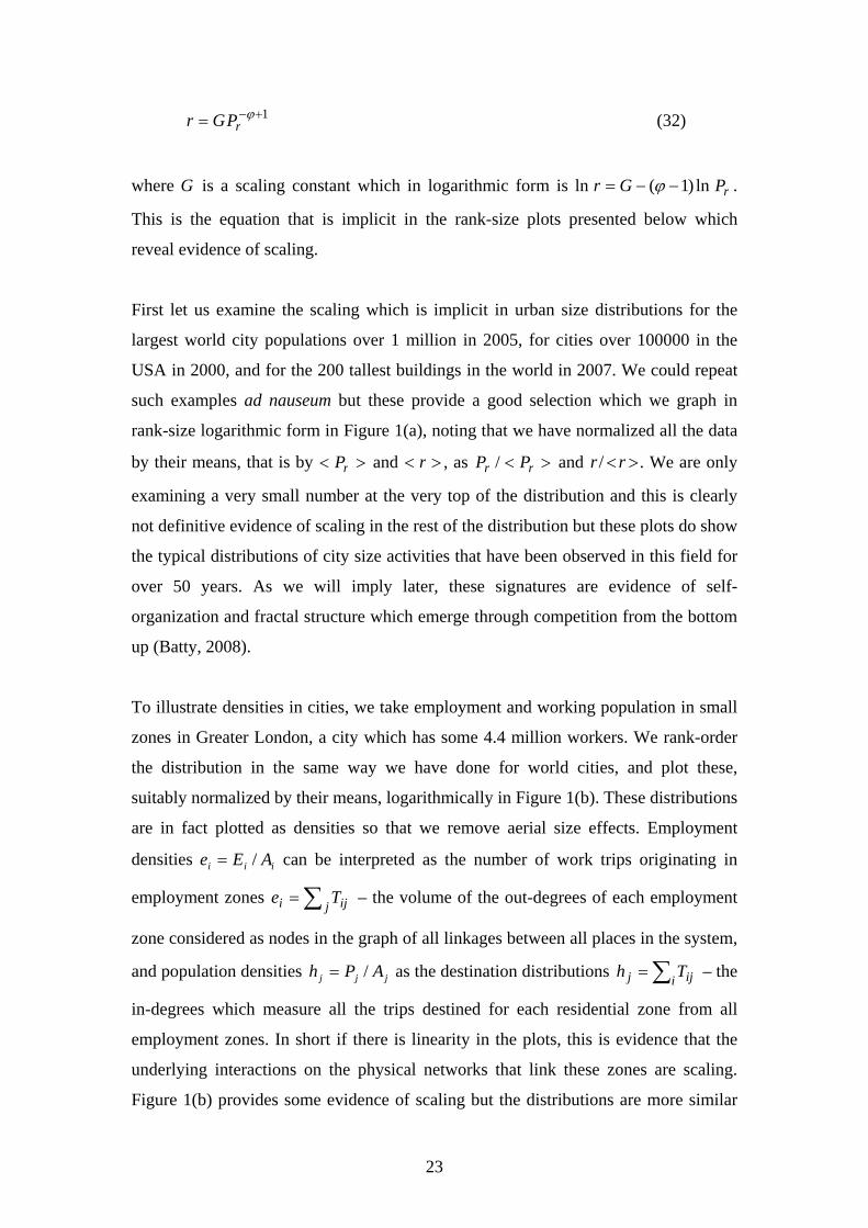
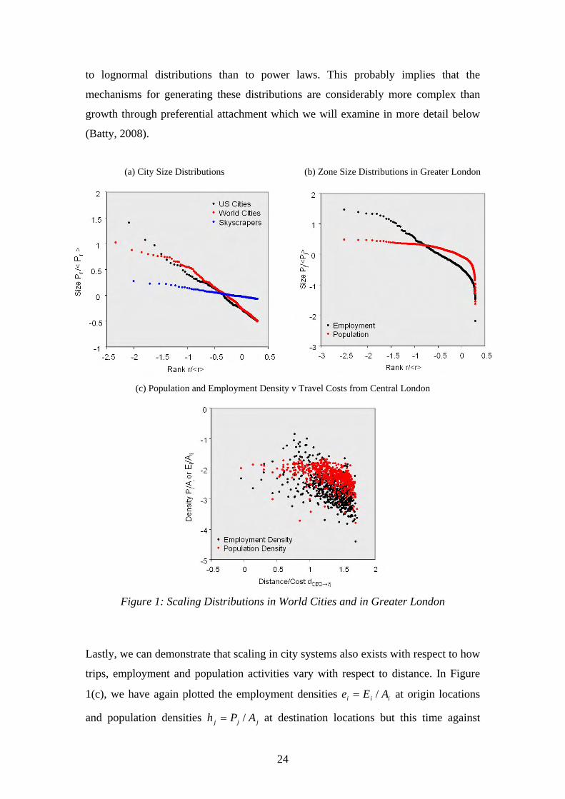
First let us examine the scaling which is implicit in urban size distributions for the

largest world city populations over 1 million in 2005, for cities over 100000 in the

USA in 2000, and for the 200 tallest buildings in the world in 2007. We could repeat

such examples ad nauseum but these provide a good selection which we graph in

rank-size logarithmic form in Figure 1(a), noting that we have normalized all the data

by their means, that is by >< rP and >< r , as >< rr PP / and ><rr / . We are only

examining a very small number at the very top of the distribution and this is clearly

not definitive evidence of scaling in the rest of the distribution but these plots do show

the typical distributions of city size activities that have been observed in this field for

over 50 years. As we will imply later, these signatures are evidence of self-

organization and fractal structure which emerge through competition from the bottom

up (Batty, 2008).

To illustrate densities in cities, we take employment and working population in small

zones in Greater London, a city which has some 4.4 million workers. We rank-order

the distribution in the same way we have done for world cities, and plot these,

suitably normalized by their means, logarithmically in Figure 1(b). These distributions

are in fact plotted as densities so that we remove aerial size effects. Employment

densities iii AEe /= can be interpreted as the number of work trips originating in

employment zones ∑= j iji Te – the volume of the out-degrees of each employment

zone considered as nodes in the graph of all linkages between all places in the system,

and population densities jjj APh /= as the destination distributions ∑= i ijj Th – the

in-degrees which measure all the trips destined for each residential zone from all

employment zones. In short if there is linearity in the plots, this is evidence that the

underlying interactions on the physical networks that link these zones are scaling.

Figure 1(b) provides some evidence of scaling but the distributions are more similar

24

to lognormal distributions than to power laws. This probably implies that the

mechanisms for generating these distributions are considerably more complex than

growth through preferential attachment which we will examine in more detail below

(Batty, 2008).

(a) City Size Distributions (b) Zone Size Distributions in Greater London

(c) Population and Employment Density v Travel Costs from Central London

Figure 1: Scaling Distributions in World Cities and in Greater London

Lastly, we can demonstrate that scaling in city systems also exists with respect to how

trips, employment and population activities vary with respect to distance. In Figure

1(c), we have again plotted the employment densities iii AEe /= at origin locations

and population densities jjj APh /= at destination locations but this time against

25

distances iCBDd → and jCBDd → from the centre of London’s CBD in logarithmic terms.

It is clear that there is significant correlation but also a very wide spread of values

around the log-linear regression lines due to the fact that the city is multi-centric.

Nevertheless the relationships appears to be scaling with these estimated as 98.0042.0 −→= iCBDi de , ( 30.02 −=r ), and 53.0029.0 −

→= jCBDj dh , ( 23.02 −=r ). However

more structured spatial relationships can be measured by accessibilities which provide

indices of overall proximity to origins or destinations, thus taking account of the fact

that there are several competing centers. Accessibility can be measured in many

different ways but here we use a traditional definition of potential based on

employment accessibility iA to populations at destinations, and population

accessibility jA to employment at origins defined as

⎪⎪

⎭

⎪⎪

⎬

⎫

∝

∝

∑

∑

i ij

ij

j ij

ji

ce

A

ch

A

, (33)

where ijc is, as before, the generalized cost of travel from employment origin i to

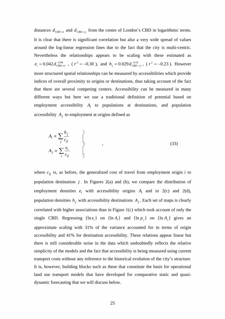
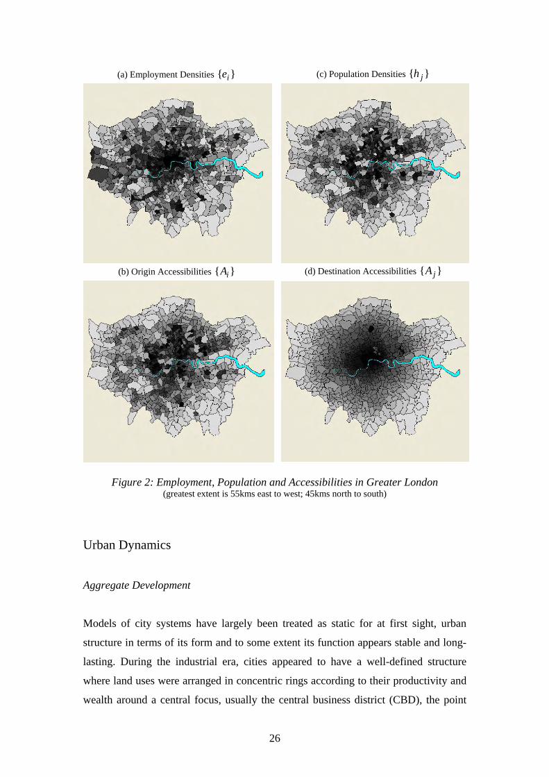
population destination j . In Figures 2(a) and (b), we compare the distribution of

employment densities ie with accessibility origins iA and in 2(c) and 2(d),

population densities jh with accessibility destinations jA . Each set of maps is clearly

correlated with higher associations than in Figure 1(c) which took account of only the

single CBD. Regressing }{ln ie on }{ln iA and }{ln jp on }{ln jA gives an

approximate scaling with 31% of the variance accounted for in terms of origin

accessibility and 41% for destination accessibility. These relations appear linear but

there is still considerable noise in the data which undoubtedly reflects the relative

simplicity of the models and the fact that accessibility is being measured using current

transport costs without any reference to the historical evolution of the city’s structure.

It is, however, building blocks such as these that constitute the basis for operational

land use transport models that have developed for comparative static and quasi-

dynamic forecasting that we will discuss below.

26

(a) Employment Densities }{ ie (c) Population Densities }{ jh

(b) Origin Accessibilities }{ iA (d) Destination Accessibilities }{ jA

Figure 2: Employment, Population and Accessibilities in Greater London

(greatest extent is 55kms east to west; 45kms north to south)

Urban Dynamics

Aggregate Development

Models of city systems have largely been treated as static for at first sight, urban

structure in terms of its form and to some extent its function appears stable and long-

lasting. During the industrial era, cities appeared to have a well-defined structure

where land uses were arranged in concentric rings according to their productivity and

wealth around a central focus, usually the central business district (CBD), the point

27

where most cities were originally located and exchange took place. Moreover data on

how cities had evolved were largely absent and this reinforced the focus on statics and

equilibria. Where the need to examine urban change was urgent, models were largely

fashioned in terms of the simplest growth dynamics possible and we will begin with

these here.

The growth of human populations in their aggregate appears to follow an exponential

law where the rate of change σ is proportional to the size of the population itself

)(tP , that is

)()( tPdt

tdP σ= . (34)

It is easy to show that starting from an initial population )0(P , the growth is

exponential, that is

)exp()0()( tPtP σ= . (35)

which is the continuous form of model. When formulated discretely, at time steps

Tt ...,,2,1= , equation (34) can be written as )1()1()( −=−− tPtPtP β which leads

to

)1()1()( −+= tPtP β . (36)

Through time from the initial condition )0(P , the trajectory is

)0()1()( PtP tβ+= . (37)

β+1 is the growth rate. If 0>β , equation (37) shows exponential growth, if 0<β ,

exponential decline, and if 0=β , the population is in the steady state and simply

reproduces itself.

28

This simple growth model leads to smooth change, and any discontinuities or breaks

in the trajectories of growth or decline must come about through an external change in

the rate from the outside environment. If we assume the growth rate fluctuates around

a mean of one with β varying randomly, above 1− , then it is not possible to predict

the trajectory of the growth path. However if we have a large number of objects which

we will assume to be cities whose growth rates are chosen randomly, then we can

write the growth equation for each city as

)1()](1[)( −+= tPttP iii β (38)

which from an initial condition )0(iP gives

)0()](1[)(1

i

t

ii PtP ∏=

+=τ

τβ . (39)

This is growth by proportionate effect; that is, each city grows in proportion to its

current size but the growth rate in each time period is random. In a large system of

cities, the ultimate distribution of these population sizes will be lognormal. This is

easy to demonstrate for the logarithm of equation (39) can be approximated by

∑=

+=t

iii PtP1

)()0(ln)(lnτ

τβ (40)

where the sum of the random components is an approximation to the log of the

product term in equation (39) using Taylor’s expansion. This converges to the

lognormal from the law of large numbers. It was first demonstrated by Gibrat (1931)

for social systems but is of considerable interest here in that the fat tail of the

lognormal can be approximated by an inverse power law. This has become the default

dynamic model which underpins an explanation of the rank-size rule for city

populations first popularized by Zipf (1949) and more recently confirmed by Gabaix

(1999) and Blank and Solomon (2000) amongst others. We demonstrated this in

Figure 1(a) for the world city populations greater than 1 million and for US city

29

populations greater than 100,000. As such, it is the null hypothesis for the distribution

of urban populations in individual cities as well as population locations within cities.

Although Gibrat’s model does not take account of interactions between the cities, it

does introduce diversity into the picture, simulating a system that in the aggregate is

non-smooth but nevertheless displays regularity. These links to aggregate dynamics

focus on introducing slightly more realistic constraints and one that is of wide

relevance is the introduction of capacity constraints or limits on the level to which a

population might grow. Such capacitated growth is usually referred to as logistic

growth. Retaining the exponential growth model, we can limit this by moderating the

growth rate σ according to an upper limit on population maxP which changes the

model in equation (34) and the growth rate σ to

)()(1)(

maxtP

PtP

dttdP

⎥⎥⎦

⎤

⎢⎢⎣

⎡⎟⎟⎠

⎞⎜⎜⎝

⎛−= σ . (41)

It is clear that when max)( PtP = , the overall rate of change is zero and no further

change occurs. The continuous version of this logistic is

)exp(1)0(

1)(

max

max

tPP

PtP

σ−⎟⎟⎠

⎞⎜⎜⎝

⎛−+

= (42)

where it is easy to see that as ∞→t , max)( PtP → .

The discrete equivalent of this model in equation (41) follows directly from

)1()]/)1((1[)1()( max −−−=−− tPPtPtPtP β as

)1()1(11)(max

−⎥⎦

⎤⎢⎣

⎡⎟⎟⎠

⎞⎜⎜⎝

⎛ −−+= tP

PtPtP β , (43)

30

where the long term dynamics is too intricate to write out as a series. Equation (43)

however shows that the growth component β is successively influenced by the

growth of the population so far, thus preserving the capacity limit through the simple

expedient of adjusting the growth rate downwards. As in all exponential models, it is

based on proportionate growth. As we noted above, we can make each city subject to

a random growth component )(tiβ while still keeping the proportionate effect.

)1()1(1)(1)(max

−⎥⎦

⎤⎢⎣

⎡⎟⎟⎠

⎞⎜⎜⎝

⎛ −−+= tP

PtPttP iβ . (44)

This model has not been tested in any detail but if )(tiβ is selected randomly, the

model is a likely to generate a lognormal-like distribution of cities but with upper

limits being invoked for some of these. In fact, this stochastic equivalent also requires

a lower integer bound on the size of cities so that cities do not become too small

(Batty, 2007). Within these limits as long as the upper limits are not too tight, the

sorts of distributions of cities that we observe in the real world are predictable.

In the case of the logistic model, remarkable and unusual discontinuous nonlinear

behavior can result from its simple dynamics. When the β component of the growth

rate is 2<β , the predicted growth trajectory is the typical logistic which increases at

an increasing rate until an inflection point after which the growth begins to slow,

eventually converging to the upper capacity limit of maxP . However when 2≅β , the

population oscillates around this limit, bifurcating between two values. As the value

of the growth rate increases towards 2.57, these oscillations get greater, the

bifurcations doubling in a regular but rapidly increasing manner. At the point where

57.2≅β , the oscillations and bifurcations become infinite, apparently random, and

this regime persists until 3≅β during which the predictions look entirely chaotic. In

fact, this is the regime of ‘chaos’ but chaos in a controlled manner from a

deterministic model which is not governed by externally induced or observed

randomness or noise.

31

These findings were found independently by May (1976), Feigenbaum (1980),

Mandelbot (1983) amongst others. They relate strongly to bifurcation and chaos

theory and to fractal geometry but they still tend to be of theoretical importance only.

Growth rates of this magnitude are rare in human systems although there is some

suggestion that they might occur in more complex coupled biological systems of

predator-prey relations. In fact one of the key issues in simulating urban systems

using this kind of dynamics is that although these models are important theoretical

constructs in defining the scope of the dynamics that define city systems, much of

these dynamic behaviors are simplistic. In so far as they do characterize urban

systems, it is at the highly aggregate scale as we demonstrate a little later. The use of

these ideas in fact is much more applicable to extending the static equilibrium models

of the last section and to demonstrate these, we will now illustrate how these models

might be enriched by putting together logistic behaviors with spatial movement and

interaction.

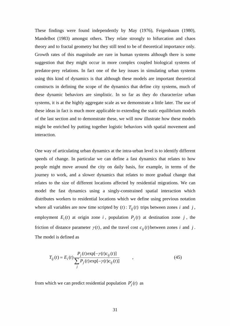
One way of articulating urban dynamics at the intra-urban level is to identify different

speeds of change. In particular we can define a fast dynamics that relates to how

people might move around the city on daily basis, for example, in terms of the

journey to work, and a slower dynamics that relates to more gradual change that

relates to the size of different locations affected by residential migrations. We can

model the fast dynamics using a singly-constrained spatial interaction which

distributes workers to residential locations which we define using previous notation

where all variables are now time scripted by )(t : )(tTij trips between zones i and j ,

employment )(tEi at origin zone i , population )(tPj at destination zone j , the

friction of distance parameter )(tγ , and the travel cost )(tcij between zones i and j .

The model is defined as

∑ −

−=

jijj

ijjiij tcttP

tcttPtEtT

)]()(exp[)()]()(exp[)(

)()(γ

γ , (45)

from which we can predict residential population )(tPj′ as

32

∑ ∑ ∑ −

−==′

i ij

ijj

ijjiijj tcttP

tcttPtEtTtP

)]()(exp[)()]()(exp[)(

)()()(γ

γ . (46)

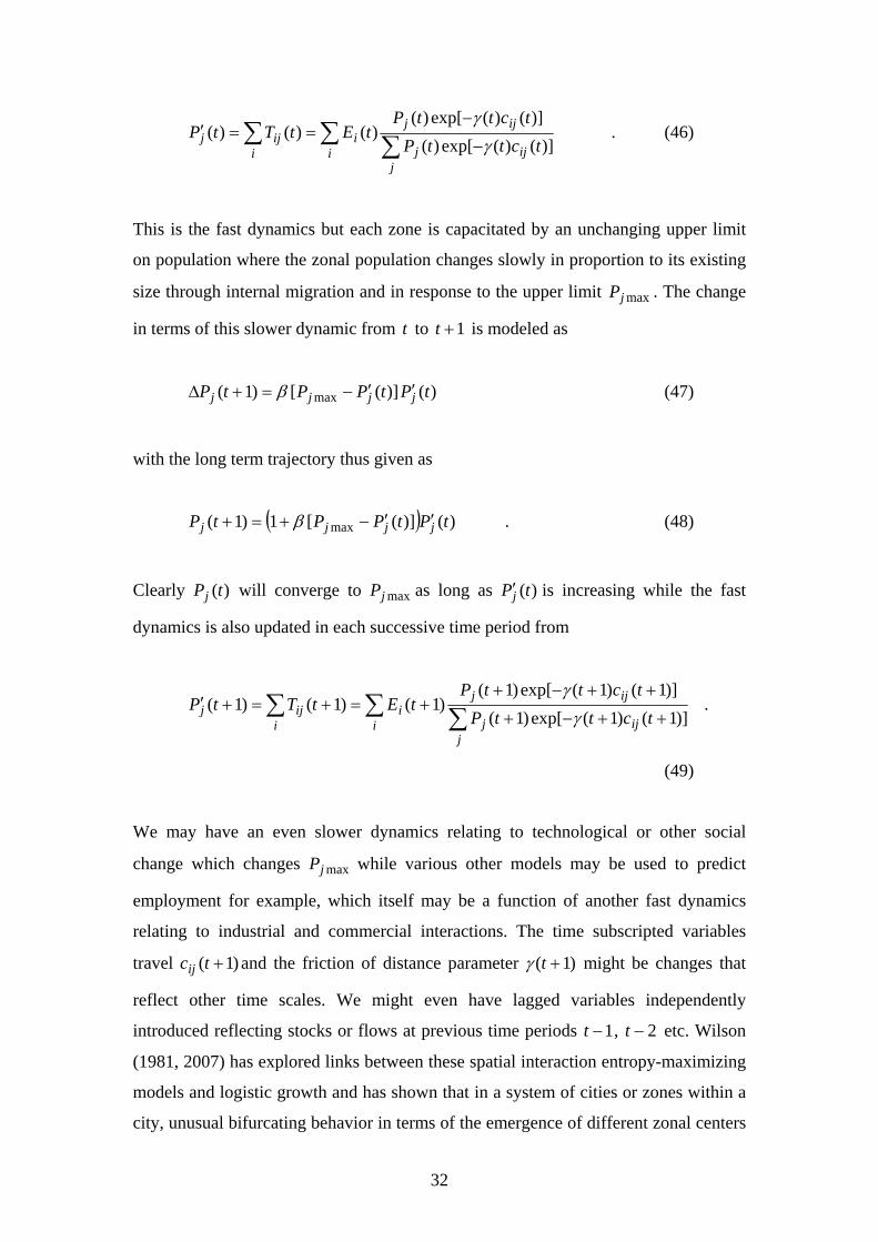
This is the fast dynamics but each zone is capacitated by an unchanging upper limit

on population where the zonal population changes slowly in proportion to its existing

size through internal migration and in response to the upper limit maxjP . The change

in terms of this slower dynamic from t to 1+t is modeled as

)()]([)1( max tPtPPtP jjjj ′′−=+Δ β (47)

with the long term trajectory thus given as

( ) )()]([1)1( max tPtPPtP jjjj ′′−+=+ β . (48)

Clearly )(tPj will converge to maxjP as long as )(tPj′ is increasing while the fast

dynamics is also updated in each successive time period from

∑ ∑ ∑ ++−+

++−++=+=+′

i ij

ijj

ijjiijj tcttP

tcttPtEtTtP

)]1()1(exp[)1()]1()1(exp[)1(

)1()1()1(γ

γ .

(49)

We may have an even slower dynamics relating to technological or other social

change which changes maxjP while various other models may be used to predict

employment for example, which itself may be a function of another fast dynamics

relating to industrial and commercial interactions. The time subscripted variables

travel )1( +tcij and the friction of distance parameter )1( +tγ might be changes that

reflect other time scales. We might even have lagged variables independently

introduced reflecting stocks or flows at previous time periods 1−t , 2−t etc. Wilson

(1981, 2007) has explored links between these spatial interaction entropy-maximizing

models and logistic growth and has shown that in a system of cities or zones within a

city, unusual bifurcating behavior in terms of the emergence of different zonal centers

33

can occur when parameter values, particularly the travel cost parameter )1( +tγ ,

crosses certain thresholds

There have been many proposals involving dynamic models of city systems which

build on the style of nonlinear dynamics introduced here and these all have the

potential to generate discontinuous behavior. Although Wilson (1981) pioneered

embedding dynamic logistic change into spatial interaction models, there have been

important extensions to urban predator-prey models by Dendrinos and Mullaly (1985)

and to bifurcating urban systems by Allen (1982, 1998), all set within a wider

dynamics linking macro to micro through master equation approaches (Haag, 1989).

A good summary is given by Nijkamp and Reggiani (1992) but most of these have not

really led to extensive empirical applications for it has been difficult to find the

necessary rich dynamics in the sparse temporal data sets available for cities and city

systems; at the macro-level, a lot of this dynamics tends to be smoothed away in any

case. In fact, more practical approaches to urban dynamics have emerged at finer

scale levels where the agents and activities are more disaggregated and where there is

a stronger relationship to spatial behavior. We will turn to these now.

Dynamic Disaggregation: Agents and Cells

Static models of the spatial interaction variety have been assembled into linked sets of

sub-models, disaggregated into detailed types of activity, and structured so that they

simulate changes in activities through time. However, the dynamics that is implied in

such models is simplistic in that the focus has still been very much on location in

space with time added as an afterthought. Temporal processes are rarely to the

forefront in such models and it is not surprising that a more flexible dynamics is

emerging from entirely different considerations. In fact, the models of this section

come from dealing with objects and individuals at much lower/finer spatial scales and

simulating processes which engage them in decisions affecting their spatial behavior.

The fact that such decisions take place through time (and space) makes them temporal

and dynamic rather through the imposition of any predetermined dynamic structures

such as those used in the aggregate dynamic models above. The models here deal with

individuals as agents, rooted in cells which define the space they occupy and in this

34

sense, are highly disaggregate as well as dynamic. These models generate

development in cities from the bottom up and have the capability of producing

patterns which are emergent. Unlike the dynamic models of the last section, their long

term spatial behavior can be surprising and often hard to anticipate.

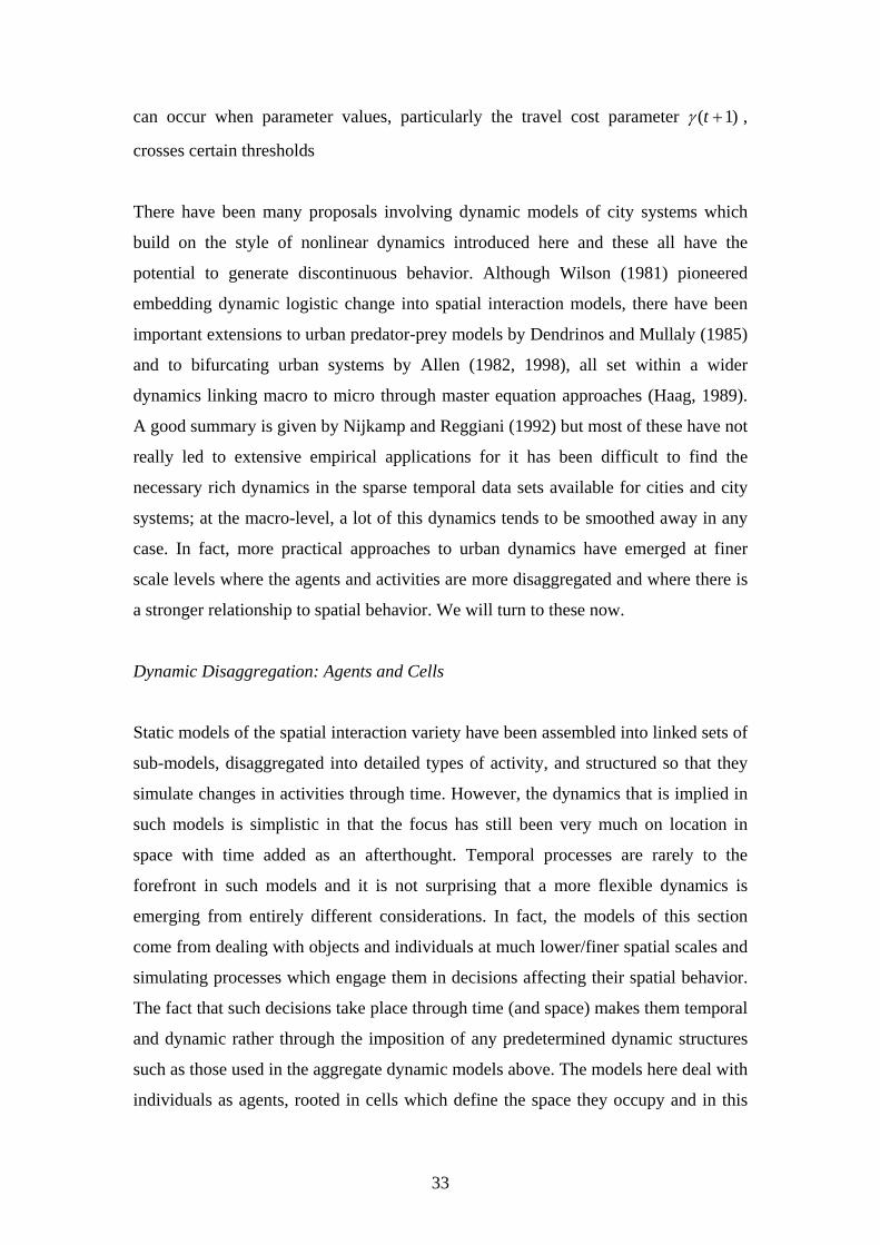
It is possible however to use the established notation for equilibrium models in

developing this framework based on the generic dynamic )()1()( tPtPtP iii Δ+−=

where the change in population )(tPiΔ can be divided into two components. The first

is the usual proportionate effect, the positive feedback induced by population on itself

which is defined as the reactive element of change )1( −tPiω . The second is the

interactive element, change that is generated from some action-at-a-distance which is

often regarded as a diffusion of population from other locations in the system. We can

model this in the simplest way using the traditional gravity model in equation (24) but

noting that we must sum the effects of the diffusion over the destinations from where

it is generated as a kind of accessibility or potential. The second component of change

is ∑ −− j ijji ctPKtP ηφ )1()1( from which the total change between t and 1−t is

)1()1(

)1()1()( −+−

−+−=Δ ∑ tc

tPKtPtPtP i

j ij

jiii εφω η . (50)

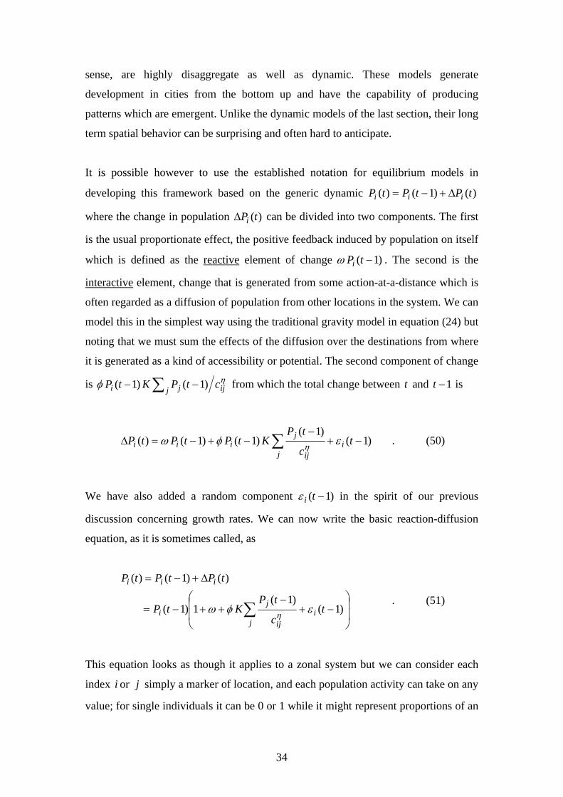
We have also added a random component )1( −tiε in the spirit of our previous

discussion concerning growth rates. We can now write the basic reaction-diffusion

equation, as it is sometimes called, as

⎟⎟

⎠

⎞

⎜⎜

⎝

⎛−+

−++−=

Δ+−=

∑j

iij

ji

iii

tc

tPKtP

tPtPtP

)1()1(

1)1(

)()1()(

εφω η

. (51)

This equation looks as though it applies to a zonal system but we can consider each

index i or j simply a marker of location, and each population activity can take on any

value; for single individuals it can be 0 or 1 while it might represent proportions of an

35

aggregate population or total numbers for the framework is entirely generic. As such,

it is more likely to mirror a slow dynamics of development rather than a fast dynamics

of movement although movement is implicit through the diffusive accessibility term.

We will therefore assume that the cells are small enough, space-wise, to contain

single activities – a single household or land use which is the cell state – with the

cellular tessellation usually forming a grid associated with the pixel map used to

visualize data input and model output. In terms of our notation, population in any cell

i must be 01)( ortPi = , representing a cell which is occupied or empty with the

change being 1)1(01)( =−−=Δ tPifortP ii and 0)1(01)( =−=Δ tPifortP ii .

These switches of state are not computed by equation (51) for the way these cellular

variants are operationalized is through a series of rules, constraints and thresholds.

Although consistent with the generic model equations, these are applied in more ad

hoc terms. Thus these models are often referred to as automata and in this case, as

cellular automata (CA).

The next simplification which determines whether or not a CA follows a strict

formalism, relates to the space over which the diffusion takes place. In the fast

dynamic equilibrium models of the last section and the slower ones of this, interaction

is usually possible across the entire space but in strict CA, diffusion is over a local

neighborhood of cells around i , iΩ , where the cells are adjacent. For symmetric

neighborhoods, the simplest is composed of cells which are north, south, east and

west of the cell in question, that is wesni ,,,=Ω – the so-called von Neumann

neighborhood, while if the diagonal nearest neighbors are included, then the number

of adjacent cells rises to 8 forming the so-called Moore neighborhood. These highly

localized neighborhoods are essential to processes that grow from the bottom up but

generate global patterns that show emergence. Rules for diffusion are based on

switching a cell’s state on or off, dependent upon what is happening in the

neighborhood, with such rules being based on counts of cells, cell attributes,

constraints on what can happen in a cell, and so on.

The simplest way of showing how diffusion in localized neighborhoods takes place

can be demonstrated by simplifying the diffusion term in equation (50) as follows.

36

Then ∑∑ −−=−j ijjj j ctPKtPK ηφφ )1()1( as 1=ijc when wesni ,,,=Ω . The cost

is set as a constant value as each cell is assumed to be small enough to incur the same

(or no) cost of transport between adjacent cells. Thus the diffusion is a count of cells

in the neighborhood i . The overall growth rate is scaled by the size of the activity in

i but this activity is always either 01)1( ortPi =− , presence or absence. In fact this

scaling is inappropriate in models that work by switching cells on and off for it is only

relevant when one is dealing with aggregates. This arises from the way the generic

equation in (51) has been derived and in CA models, it is assumed to be neutral. Thus

the change equation (50) becomes

)()1()( ttPKtP ij

ji εφω +−+=Δ ∑ , (52)

where this can now be used to determine a threshold maxZ over which the cell state is

switched. A typical rule might be

⎪⎩

⎪⎨⎧ >+−+

=∑

otherwise

ZttPKiftP

ij

ji

,0

)]()1([1)(

maxεφω . (53)

It is entirely possible to separate the reaction from the diffusion and consider different

combinations of these effects sparking off a state change. As we have implied,

different combinations of attributes in cells and constraints within neighborhoods can

be used to effect a switch, much depending on the precise specification of the model.

In many growth models based on CA, the strict limits posed by a local neighborhood

are relaxed. In short, the diffusion field is no longer local but is an information or

potential field consistent with its use in social physics where action-at-distance is

assumed to be all important. In the case of strict CA, it is assumed that there is no

action-at-a-distance in that diffusion only takes place to physically adjacent cells.

Over time, activity can reach all parts of the system but it cannot hop over the basic

cell unit. In cities, this is clearly quite unrealistic as the feasibility of deciding what

and where to locate does not depend on physical adjacency. In terms of applications,

37

there are few if any urban growth models based on strict CA although this does rather

beg the question as to why CA is being used in the first place. In fact it is more

appropriate to call such models cell-space or CS models as Couclelis (1985) has

suggested. In another sense, this framework can be considered as one for agent-based

modeling where the cells are not agents and where there is no assumption of a regular

underlying grid of cells (Batty, 2005a, 2005b). There may be such a grid but the

framework simply supposes that the indices i and j refer to locations that may form

a regular tessellation but alternatively may be mobile and changing. In such cases, it is

often necessary to extend the notation to deal with specific relations between the

underlying space and the location of each agent.

Empirical Dynamics: Population Change and City Size

We will now briefly illustrate examples of the models introduced in this section

before we then examine the construction of more comprehensive models of city

systems. Simple exponential growth models apply to rapidly growing populations

which are nowhere near capacity limits such as entire countries or the world. In

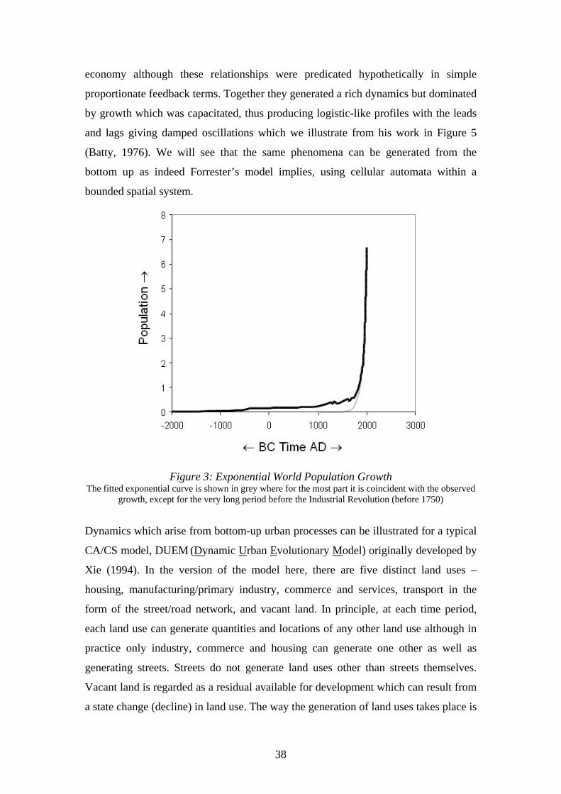
Figure 3, we show the growth of world population from 2000 BCE to date where it is

clear that the rate of growth may be faster than the exponential model implies,

although probably not as fast as double exponential. In fact world population is likely

to slow rapidly over the next century probably mirroring global resource limits to an

extent which are clearly illustrated in the growth of the largest western cities. In

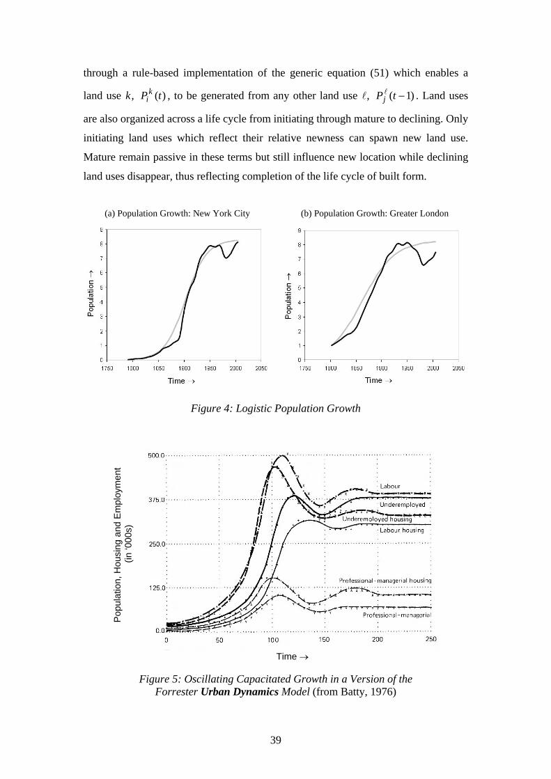
Figures 4(a) and 4(b), we show the growth in population of New York City (the five

boroughs) and Greater London from 1750 to date and it is clear that in both cases, as

the cities developed, population grew exponentially only to slow as the upper density

limits of each city were reached.

Subsequent population loss and then a recent return of population to the inner and

central city now dominate these two urban cores, which is reminiscent of the sorts of

urban dynamic simulated by Forrester (1969) where various leads and lags in the flow

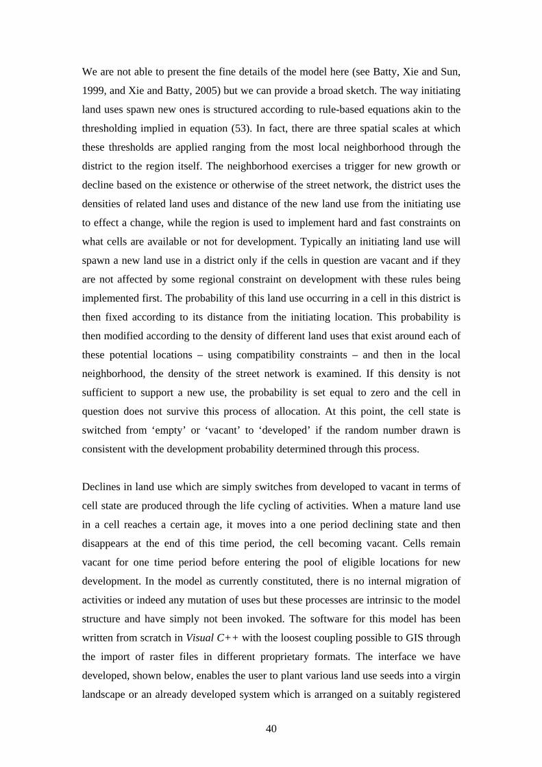
of populations mean that the capacity limit is often overshot, setting up a series of

oscillations which damp in the limit. Forrester’s model was the one of the first to

grapple with the many interconnections between stocks and flows in the urban

38

economy although these relationships were predicated hypothetically in simple

proportionate feedback terms. Together they generated a rich dynamics but dominated

by growth which was capacitated, thus producing logistic-like profiles with the leads

and lags giving damped oscillations which we illustrate from his work in Figure 5

(Batty, 1976). We will see that the same phenomena can be generated from the

bottom up as indeed Forrester’s model implies, using cellular automata within a

bounded spatial system.

Figure 3: Exponential World Population Growth The fitted exponential curve is shown in grey where for the most part it is coincident with the observed

growth, except for the very long period before the Industrial Revolution (before 1750)

Dynamics which arise from bottom-up urban processes can be illustrated for a typical

CA/CS model, DUEM (Dynamic Urban Evolutionary Model) originally developed by

Xie (1994). In the version of the model here, there are five distinct land uses –

housing, manufacturing/primary industry, commerce and services, transport in the

form of the street/road network, and vacant land. In principle, at each time period,

each land use can generate quantities and locations of any other land use although in

practice only industry, commerce and housing can generate one other as well as

generating streets. Streets do not generate land uses other than streets themselves.

Vacant land is regarded as a residual available for development which can result from

a state change (decline) in land use. The way the generation of land uses takes place is

39

through a rule-based implementation of the generic equation (51) which enables a

land use ,k )(tPki , to be generated from any other land use ,l )1( −tPj

l . Land uses

are also organized across a life cycle from initiating through mature to declining. Only

initiating land uses which reflect their relative newness can spawn new land use.

Mature remain passive in these terms but still influence new location while declining

land uses disappear, thus reflecting completion of the life cycle of built form.

(a) Population Growth: New York City (b) Population Growth: Greater London

Figure 4: Logistic Population Growth

Pop

ulat

ion,

Hou

sing

and

Em

ploy

men

t (i

n ‘0

00s)

Time →

Figure 5: Oscillating Capacitated Growth in a Version of the

Forrester Urban Dynamics Model (from Batty, 1976)

40

We are not able to present the fine details of the model here (see Batty, Xie and Sun,

1999, and Xie and Batty, 2005) but we can provide a broad sketch. The way initiating

land uses spawn new ones is structured according to rule-based equations akin to the

thresholding implied in equation (53). In fact, there are three spatial scales at which

these thresholds are applied ranging from the most local neighborhood through the

district to the region itself. The neighborhood exercises a trigger for new growth or

decline based on the existence or otherwise of the street network, the district uses the

densities of related land uses and distance of the new land use from the initiating use

to effect a change, while the region is used to implement hard and fast constraints on

what cells are available or not for development. Typically an initiating land use will

spawn a new land use in a district only if the cells in question are vacant and if they

are not affected by some regional constraint on development with these rules being

implemented first. The probability of this land use occurring in a cell in this district is

then fixed according to its distance from the initiating location. This probability is

then modified according to the density of different land uses that exist around each of

these potential locations – using compatibility constraints – and then in the local

neighborhood, the density of the street network is examined. If this density is not

sufficient to support a new use, the probability is set equal to zero and the cell in

question does not survive this process of allocation. At this point, the cell state is

switched from ‘empty’ or ‘vacant’ to ‘developed’ if the random number drawn is

consistent with the development probability determined through this process.

Declines in land use which are simply switches from developed to vacant in terms of

cell state are produced through the life cycling of activities. When a mature land use

in a cell reaches a certain age, it moves into a one period declining state and then

disappears at the end of this time period, the cell becoming vacant. Cells remain

vacant for one time period before entering the pool of eligible locations for new

development. In the model as currently constituted, there is no internal migration of

activities or indeed any mutation of uses but these processes are intrinsic to the model

structure and have simply not been invoked. The software for this model has been

written from scratch in Visual C++ with the loosest coupling possible to GIS through

the import of raster files in different proprietary formats. The interface we have

developed, shown below, enables the user to plant various land use seeds into a virgin

landscape or an already developed system which is arranged on a suitably registered

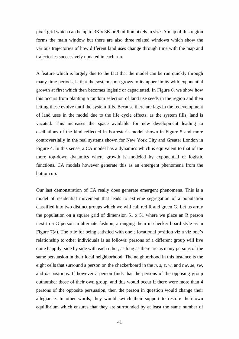
41

pixel grid which can be up to 3K x 3K or 9 million pixels in size. A map of this region

forms the main window but there are also three related windows which show the

various trajectories of how different land uses change through time with the map and

trajectories successively updated in each run.

A feature which is largely due to the fact that the model can be run quickly through

many time periods, is that the system soon grows to its upper limits with exponential

growth at first which then becomes logistic or capacitated. In Figure 6, we show how

this occurs from planting a random selection of land use seeds in the region and then

letting these evolve until the system fills. Because there are lags in the redevelopment

of land uses in the model due to the life cycle effects, as the system fills, land is

vacated. This increases the space available for new development leading to

oscillations of the kind reflected in Forrester’s model shown in Figure 5 and more

controversially in the real systems shown for New York City and Greater London in

Figure 4. In this sense, a CA model has a dynamics which is equivalent to that of the

more top-down dynamics where growth is modeled by exponential or logistic

functions. CA models however generate this as an emergent phenomena from the

bottom up.

Our last demonstration of CA really does generate emergent phenomena. This is a

model of residential movement that leads to extreme segregation of a population

classified into two distinct groups which we will call red R and green G. Let us array

the population on a square grid of dimension 51 x 51 where we place an R person

next to a G person in alternate fashion, arranging them in checker board style as in

Figure 7(a). The rule for being satisfied with one’s locational position viz a viz one’s

relationship to other individuals is as follows: persons of a different group will live

quite happily, side by side with each other, as long as there are as many persons of the

same persuasion in their local neighborhood. The neighborhood in this instance is the

eight cells that surround a person on the checkerboard in the n, s, e, w, and nw, se, sw,

and ne positions. If however a person finds that the persons of the opposing group

outnumber those of their own group, and this would occur if there were more than 4

persons of the opposite persuasion, then the person in question would change their

allegiance. In other words, they would switch their support to restore their own

equilibrium which ensures that they are surrounded by at least the same number of

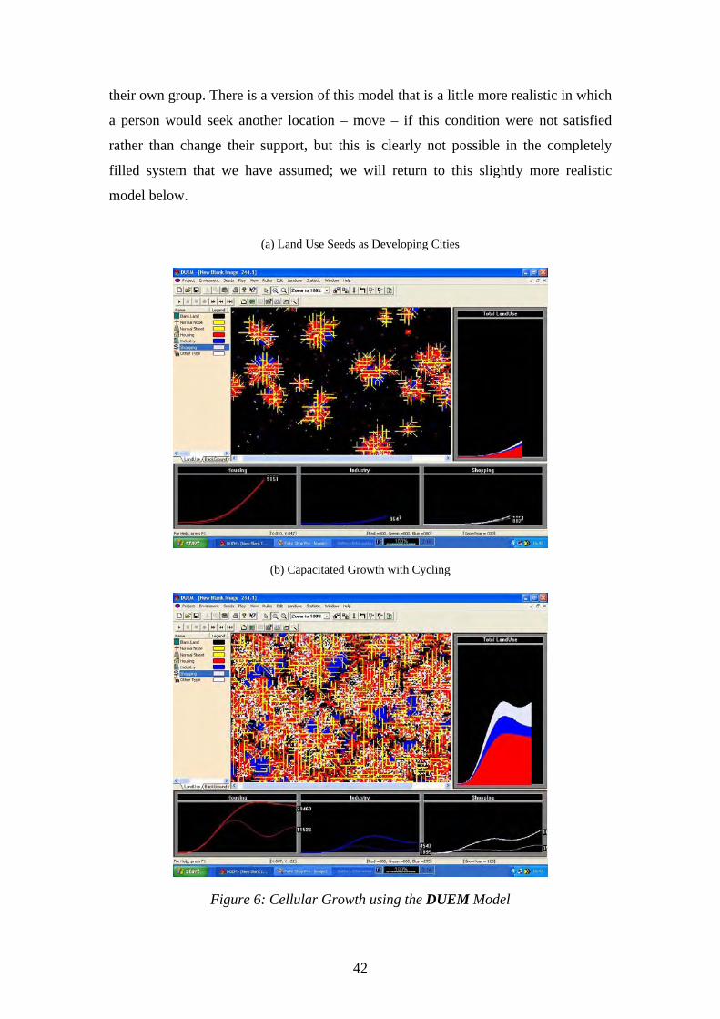
42

their own group. There is a version of this model that is a little more realistic in which

a person would seek another location – move – if this condition were not satisfied

rather than change their support, but this is clearly not possible in the completely

filled system that we have assumed; we will return to this slightly more realistic

model below.

(a) Land Use Seeds as Developing Cities

(b) Capacitated Growth with Cycling

Figure 6: Cellular Growth using the DUEM Model

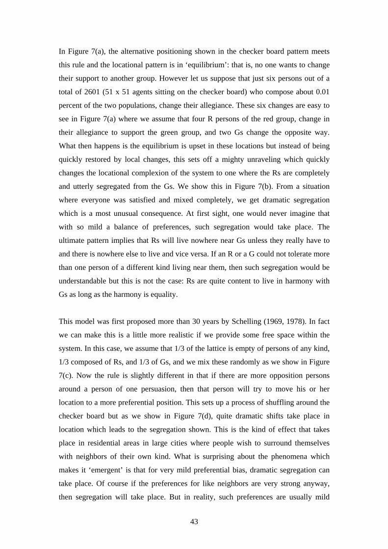
43

In Figure 7(a), the alternative positioning shown in the checker board pattern meets

this rule and the locational pattern is in ‘equilibrium’: that is, no one wants to change

their support to another group. However let us suppose that just six persons out of a

total of 2601 (51 x 51 agents sitting on the checker board) who compose about 0.01

percent of the two populations, change their allegiance. These six changes are easy to

see in Figure 7(a) where we assume that four R persons of the red group, change in

their allegiance to support the green group, and two Gs change the opposite way.

What then happens is the equilibrium is upset in these locations but instead of being

quickly restored by local changes, this sets off a mighty unraveling which quickly

changes the locational complexion of the system to one where the Rs are completely

and utterly segregated from the Gs. We show this in Figure 7(b). From a situation

where everyone was satisfied and mixed completely, we get dramatic segregation

which is a most unusual consequence. At first sight, one would never imagine that

with so mild a balance of preferences, such segregation would take place. The

ultimate pattern implies that Rs will live nowhere near Gs unless they really have to

and there is nowhere else to live and vice versa. If an R or a G could not tolerate more

than one person of a different kind living near them, then such segregation would be

understandable but this is not the case: Rs are quite content to live in harmony with

Gs as long as the harmony is equality.

This model was first proposed more than 30 years by Schelling (1969, 1978). In fact

we can make this is a little more realistic if we provide some free space within the

system. In this case, we assume that 1/3 of the lattice is empty of persons of any kind,

1/3 composed of Rs, and 1/3 of Gs, and we mix these randomly as we show in Figure

7(c). Now the rule is slightly different in that if there are more opposition persons

around a person of one persuasion, then that person will try to move his or her

location to a more preferential position. This sets up a process of shuffling around the

checker board but as we show in Figure 7(d), quite dramatic shifts take place in

location which leads to the segregation shown. This is the kind of effect that takes

place in residential areas in large cities where people wish to surround themselves

with neighbors of their own kind. What is surprising about the phenomena which

makes it ‘emergent’ is that for very mild preferential bias, dramatic segregation can

take place. Of course if the preferences for like neighbors are very strong anyway,

then segregation will take place. But in reality, such preferences are usually mild

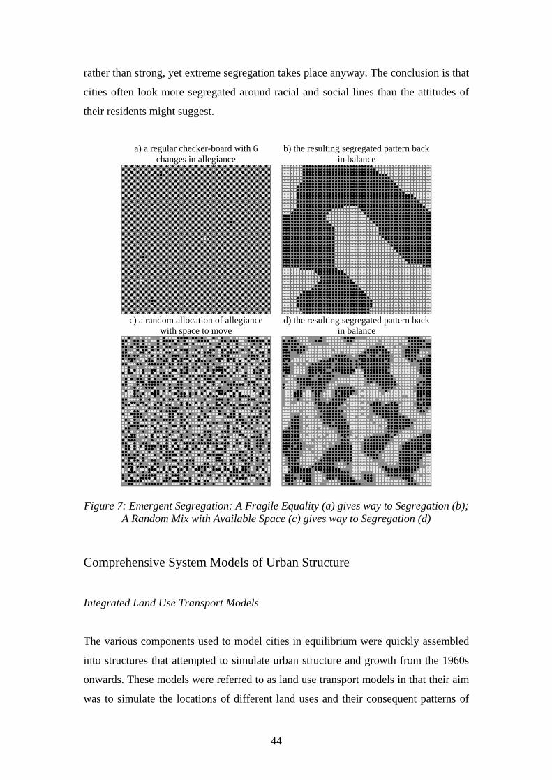
44

rather than strong, yet extreme segregation takes place anyway. The conclusion is that

cities often look more segregated around racial and social lines than the attitudes of

their residents might suggest.

a) a regular checker-board with 6

changes in allegiance b) the resulting segregated pattern back

in balance

c) a random allocation of allegiance

with space to move d) the resulting segregated pattern back

in balance

Figure 7: Emergent Segregation: A Fragile Equality (a) gives way to Segregation (b);

A Random Mix with Available Space (c) gives way to Segregation (d)

Comprehensive System Models of Urban Structure

Integrated Land Use Transport Models

The various components used to model cities in equilibrium were quickly assembled

into structures that attempted to simulate urban structure and growth from the 1960s

onwards. These models were referred to as land use transport models in that their aim

was to simulate the locations of different land uses and their consequent patterns of

45

traffic generation, usually according to spatial interaction principles based on

gravitational assumptions. But they usually represented cities as demographic and

economic activities – population, households, employment and so on – rather than as

residential, commercial or industrial land use. In short the city system was seen to

operate at the level of the location of activities which then consumed space through

land use from which traffic was generated, and once urban activities and their

interactions were predicted, appropriate translations were made into land use. As we

shall see, this is not as unproblematic as was originally thought.

The integration of urban activities and their interactions – land use and transport – can

be accomplished using a variety of economic frameworks built around economic

relationships between activities. Traditionally these have been represented as input-

output models where one activity is linked to another and it is possible to predict the

chain of linkages between all the activities using multipliers. We will illustrate this for

two activities: we assume that employment E is divided into an unpredictable

component, sometimes considered as employment that is basic B and export

orientated in the economy, and employment that is non-basic S where SBE += .

Non-basic employment services the population P from which it is derived as bPS = .

If we then consider that population can be generated by applying an activity rate a to

employment as EaP = , we have the rudiments of a generative sequence that forms a

structure for predicting activities and their locations which are highly interdependent.

Simple manipulation of these relationships shows that 1)1( −−= baBE where

1)1( −− ba is the multiplier central to traditional macro-economic theory.

If we now consider that employment and population are related spatially through their

interactions, we model the relationship between employment as population using a

singly-constrained sub-model

∑∑∑ −

−

==k ikk

ijj

ii

iijj

cF

cFEaTaP ψ

ψ

, . (54)

46

where ijT are work trips between i and j , jF is some measure of attraction at

residential location j , and ψ is the friction of distance/travel cost parameter.

Employment is modeled in reverse direction as

∑∑∑ −

−

==k kik

jii

jj

jjii cF

cFPbSbE ϖ

ϖ

, (55)

where jiS are employment demands in j from i , iF is some measure of attraction at

residential location i , and ϖ is the friction of distance/travel cost parameter. These

two equations for the two sectors are not usually solved simultaneously but the chain

is broken in that we start with basic employment B in equation (54), predicting basic

population, then using this basic population in equation (55) to produce an increment

of non-basic employment which in turn is used to predict the next increment of non-

basic population in equation (54). This iteration converges to the multiplier

relationships 1)1( −−= baBE and 1)1( −−= babBP .

This kind of sequence can be disaggregated indefinitely with respect to population

and employment types and linked demands to other sectors. Education, leisure and so

on can be added to the framework making the model ever more comprehensive. This

was the model first developed by Lowry (1964). It is still the most widely applied of

all operational urban models and has been elaborated in various ways, some of them

dealing with partial dynamics (Batty, 1976). Their theoretical pedigree is rooted

largely in regional economics, location theory and the new urban economics which

represent the spatial equivalents of classical macro and micro economics. The most

coherent recent statement in this vein is based on applications of trade theory to the

urban economy as reflected in the work of Fujita, Krugman and Venables (1999) but

there is a long heritage of empirical models in the Lowry (1964) tradition which

continue to be built (Wegener, 2005).

These models now incorporate the four-stage transportation modeling process of trip

generation, distribution, modal split and assignment explicitly and they are consistent

with discrete choice methods based on utility maximizing in their simulation of trip-

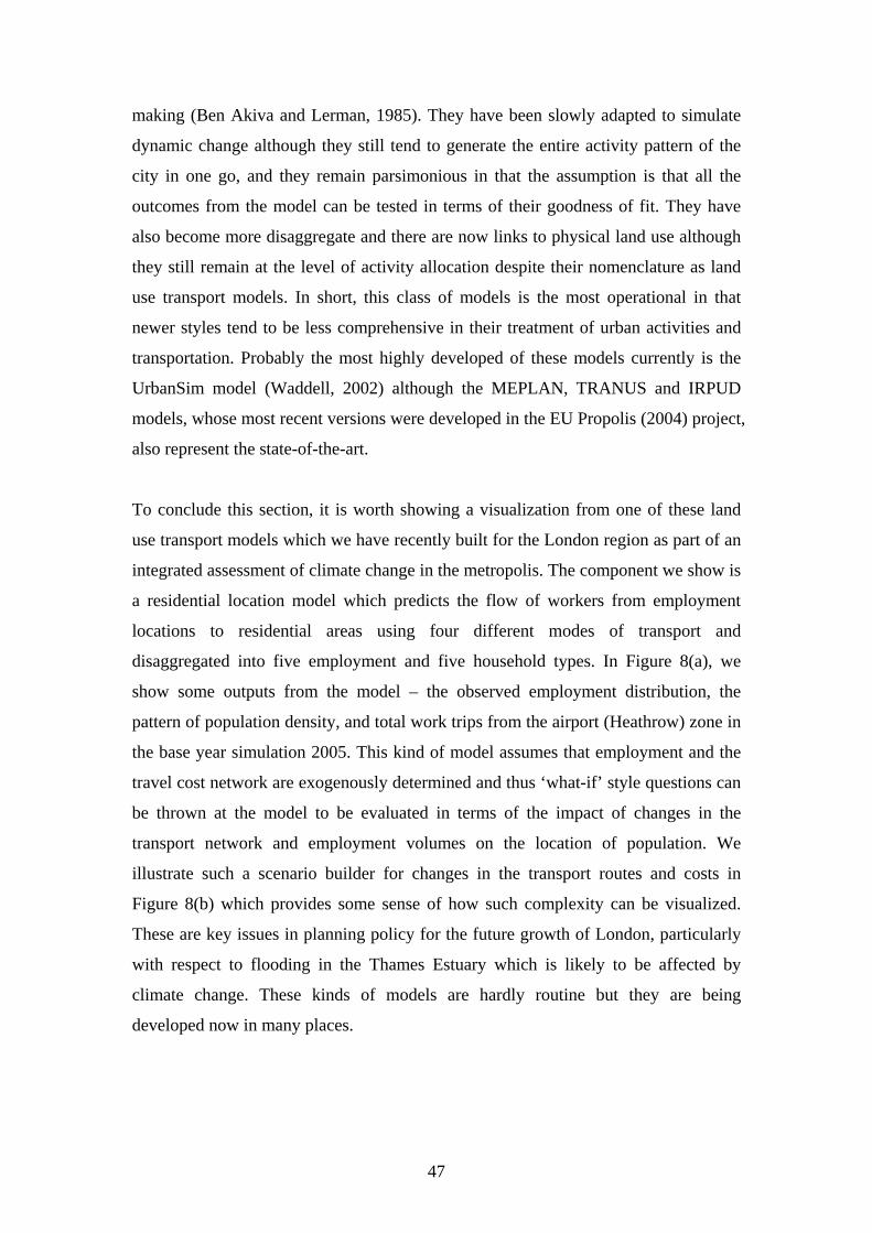
47

making (Ben Akiva and Lerman, 1985). They have been slowly adapted to simulate

dynamic change although they still tend to generate the entire activity pattern of the

city in one go, and they remain parsimonious in that the assumption is that all the

outcomes from the model can be tested in terms of their goodness of fit. They have

also become more disaggregate and there are now links to physical land use although

they still remain at the level of activity allocation despite their nomenclature as land

use transport models. In short, this class of models is the most operational in that

newer styles tend to be less comprehensive in their treatment of urban activities and

transportation. Probably the most highly developed of these models currently is the

UrbanSim model (Waddell, 2002) although the MEPLAN, TRANUS and IRPUD

models, whose most recent versions were developed in the EU Propolis (2004) project,

also represent the state-of-the-art.

To conclude this section, it is worth showing a visualization from one of these land

use transport models which we have recently built for the London region as part of an

integrated assessment of climate change in the metropolis. The component we show is

a residential location model which predicts the flow of workers from employment

locations to residential areas using four different modes of transport and

disaggregated into five employment and five household types. In Figure 8(a), we

show some outputs from the model – the observed employment distribution, the

pattern of population density, and total work trips from the airport (Heathrow) zone in

the base year simulation 2005. This kind of model assumes that employment and the

travel cost network are exogenously determined and thus ‘what-if’ style questions can

be thrown at the model to be evaluated in terms of the impact of changes in the

transport network and employment volumes on the location of population. We

illustrate such a scenario builder for changes in the transport routes and costs in

Figure 8(b) which provides some sense of how such complexity can be visualized.

These are key issues in planning policy for the future growth of London, particularly

with respect to flooding in the Thames Estuary which is likely to be affected by

climate change. These kinds of models are hardly routine but they are being

developed now in many places.

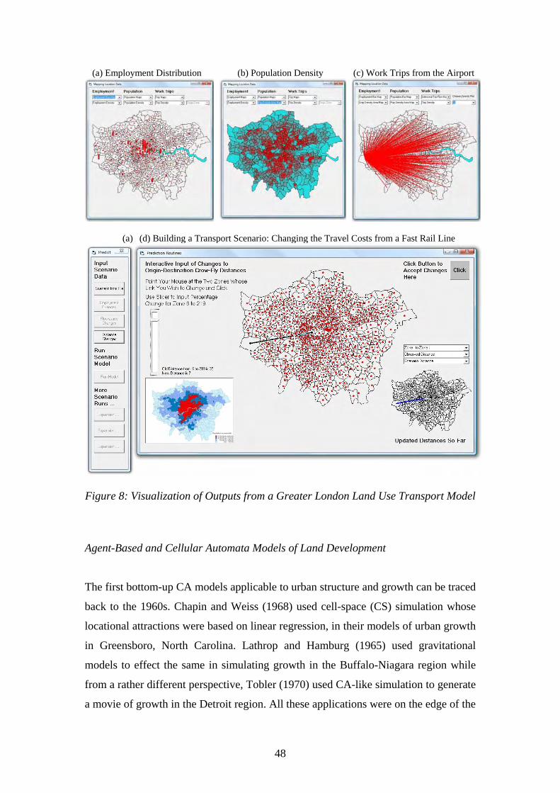
48

(a) Employment Distribution (b) Population Density (c) Work Trips from the Airport

(a) (d) Building a Transport Scenario: Changing the Travel Costs from a Fast Rail Line

Figure 8: Visualization of Outputs from a Greater London Land Use Transport Model

Agent-Based and Cellular Automata Models of Land Development

The first bottom-up CA models applicable to urban structure and growth can be traced

back to the 1960s. Chapin and Weiss (1968) used cell-space (CS) simulation whose

locational attractions were based on linear regression, in their models of urban growth

in Greensboro, North Carolina. Lathrop and Hamburg (1965) used gravitational

models to effect the same in simulating growth in the Buffalo-Niagara region while

from a rather different perspective, Tobler (1970) used CA-like simulation to generate

a movie of growth in the Detroit region. All these applications were on the edge of the

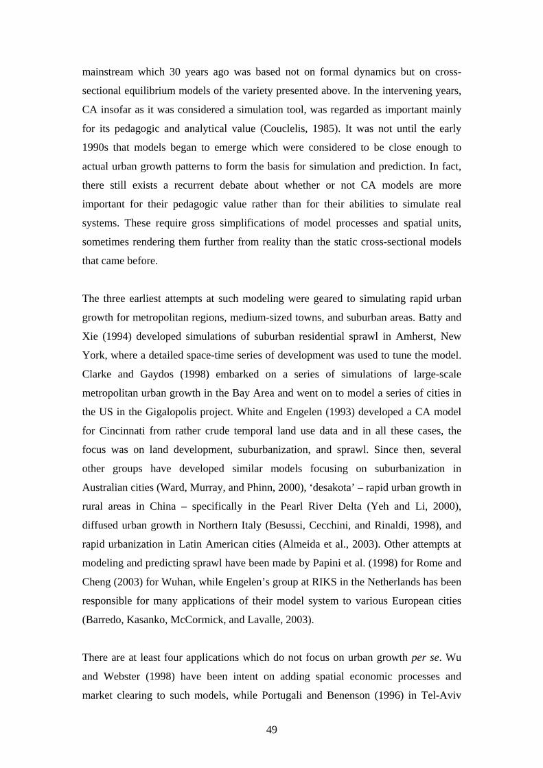
49

mainstream which 30 years ago was based not on formal dynamics but on cross-

sectional equilibrium models of the variety presented above. In the intervening years,

CA insofar as it was considered a simulation tool, was regarded as important mainly

for its pedagogic and analytical value (Couclelis, 1985). It was not until the early

1990s that models began to emerge which were considered to be close enough to

actual urban growth patterns to form the basis for simulation and prediction. In fact,

there still exists a recurrent debate about whether or not CA models are more

important for their pedagogic value rather than for their abilities to simulate real

systems. These require gross simplifications of model processes and spatial units,

sometimes rendering them further from reality than the static cross-sectional models

that came before.

The three earliest attempts at such modeling were geared to simulating rapid urban

growth for metropolitan regions, medium-sized towns, and suburban areas. Batty and

Xie (1994) developed simulations of suburban residential sprawl in Amherst, New

York, where a detailed space-time series of development was used to tune the model.

Clarke and Gaydos (1998) embarked on a series of simulations of large-scale

metropolitan urban growth in the Bay Area and went on to model a series of cities in

the US in the Gigalopolis project. White and Engelen (1993) developed a CA model

for Cincinnati from rather crude temporal land use data and in all these cases, the

focus was on land development, suburbanization, and sprawl. Since then, several

other groups have developed similar models focusing on suburbanization in

Australian cities (Ward, Murray, and Phinn, 2000), ‘desakota’ – rapid urban growth in

rural areas in China – specifically in the Pearl River Delta (Yeh and Li, 2000),

diffused urban growth in Northern Italy (Besussi, Cecchini, and Rinaldi, 1998), and

rapid urbanization in Latin American cities (Almeida et al., 2003). Other attempts at

modeling and predicting sprawl have been made by Papini et al. (1998) for Rome and

Cheng (2003) for Wuhan, while Engelen’s group at RIKS in the Netherlands has been

responsible for many applications of their model system to various European cities

(Barredo, Kasanko, McCormick, and Lavalle, 2003).

There are at least four applications which do not focus on urban growth per se. Wu

and Webster (1998) have been intent on adding spatial economic processes and

market clearing to such models, while Portugali and Benenson (1996) in Tel-Aviv

50

have focused their efforts on intra-urban change, particularly segregation and

ghettoization. Semboloni (2000) has worked on adding more classical mechanisms to

his CA models reflecting scale and hierarchy as well as extending his simulations to

the third dimension, while there have been several attempts by physicists to evolve a

more general CA framework for urban development which links to new ideas in

complexity such as self-organized criticality and power law scaling (Andersson,

Rasmussen, and White, 2002; Schweitzer and Steinbrink, 1997).

Figure 9: Simulating Very Slow Growth and Rapid Decline in the Detroit Region Using the CA DUEM Model

It is worth showing some graphics from such CA models as they are being applied to

real cities. In Figure 9, we show how the DUEM model can be used to simulate the

pattern of development change in the Detroit region of South East Michigan. In a

sense because we live in world dominated by a somewhat unhealthy interest in growth,

it might be assumed that all the models we have presented here are only geared to

simulating new development. In fact, each of these models can simulate decline or

reproduce the steady state because CA models can solely deal with transitions and

change in the existing fabric as we illustrated earlier in the Schelling segregation

model. This is the case in Detroit where the population has rapidly adjusted and

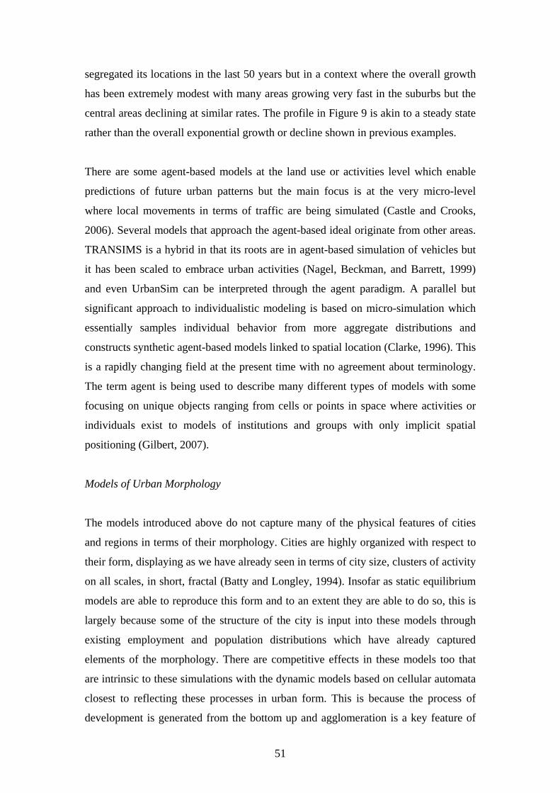
51

segregated its locations in the last 50 years but in a context where the overall growth

has been extremely modest with many areas growing very fast in the suburbs but the

central areas declining at similar rates. The profile in Figure 9 is akin to a steady state

rather than the overall exponential growth or decline shown in previous examples.

There are some agent-based models at the land use or activities level which enable

predictions of future urban patterns but the main focus is at the very micro-level

where local movements in terms of traffic are being simulated (Castle and Crooks,

2006). Several models that approach the agent-based ideal originate from other areas.

TRANSIMS is a hybrid in that its roots are in agent-based simulation of vehicles but

it has been scaled to embrace urban activities (Nagel, Beckman, and Barrett, 1999)

and even UrbanSim can be interpreted through the agent paradigm. A parallel but

significant approach to individualistic modeling is based on micro-simulation which

essentially samples individual behavior from more aggregate distributions and

constructs synthetic agent-based models linked to spatial location (Clarke, 1996). This

is a rapidly changing field at the present time with no agreement about terminology.

The term agent is being used to describe many different types of models with some

focusing on unique objects ranging from cells or points in space where activities or

individuals exist to models of institutions and groups with only implicit spatial

positioning (Gilbert, 2007).

Models of Urban Morphology

The models introduced above do not capture many of the physical features of cities

and regions in terms of their morphology. Cities are highly organized with respect to

their form, displaying as we have already seen in terms of city size, clusters of activity

on all scales, in short, fractal (Batty and Longley, 1994). Insofar as static equilibrium

models are able to reproduce this form and to an extent they are able to do so, this is

largely because some of the structure of the city is input into these models through

existing employment and population distributions which have already captured

elements of the morphology. There are competitive effects in these models too that

are intrinsic to these simulations with the dynamic models based on cellular automata

closest to reflecting these processes in urban form. This is because the process of

development is generated from the bottom up and agglomeration is a key feature of

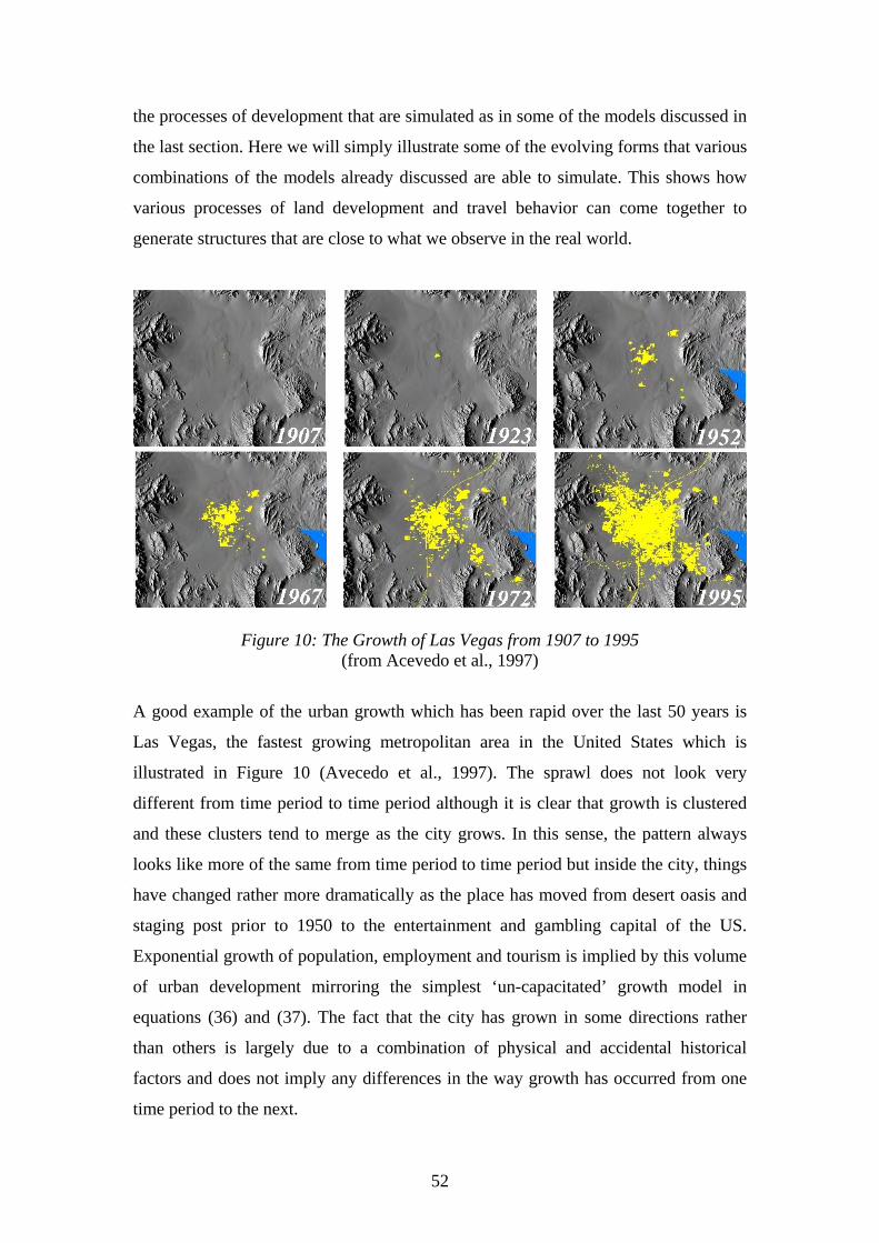
52

the processes of development that are simulated as in some of the models discussed in

the last section. Here we will simply illustrate some of the evolving forms that various

combinations of the models already discussed are able to simulate. This shows how

various processes of land development and travel behavior can come together to

generate structures that are close to what we observe in the real world.

Figure 10: The Growth of Las Vegas from 1907 to 1995 (from Acevedo et al., 1997)

A good example of the urban growth which has been rapid over the last 50 years is

Las Vegas, the fastest growing metropolitan area in the United States which is

illustrated in Figure 10 (Avecedo et al., 1997). The sprawl does not look very

different from time period to time period although it is clear that growth is clustered

and these clusters tend to merge as the city grows. In this sense, the pattern always

looks like more of the same from time period to time period but inside the city, things

have changed rather more dramatically as the place has moved from desert oasis and

staging post prior to 1950 to the entertainment and gambling capital of the US.

Exponential growth of population, employment and tourism is implied by this volume

of urban development mirroring the simplest ‘un-capacitated’ growth model in

equations (36) and (37). The fact that the city has grown in some directions rather

than others is largely due to a combination of physical and accidental historical

factors and does not imply any differences in the way growth has occurred from one

time period to the next.

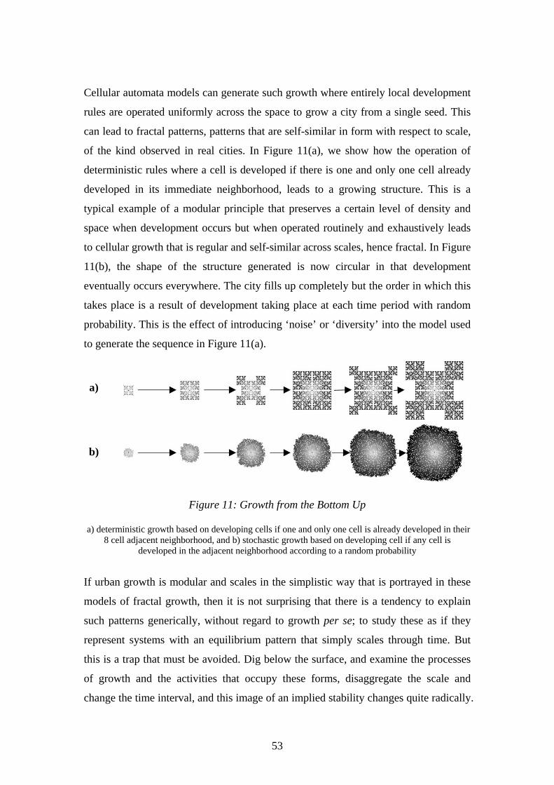
53

Cellular automata models can generate such growth where entirely local development

rules are operated uniformly across the space to grow a city from a single seed. This

can lead to fractal patterns, patterns that are self-similar in form with respect to scale,

of the kind observed in real cities. In Figure 11(a), we show how the operation of

deterministic rules where a cell is developed if there is one and only one cell already

developed in its immediate neighborhood, leads to a growing structure. This is a

typical example of a modular principle that preserves a certain level of density and

space when development occurs but when operated routinely and exhaustively leads

to cellular growth that is regular and self-similar across scales, hence fractal. In Figure

11(b), the shape of the structure generated is now circular in that development

eventually occurs everywhere. The city fills up completely but the order in which this

takes place is a result of development taking place at each time period with random

probability. This is the effect of introducing ‘noise’ or ‘diversity’ into the model used

to generate the sequence in Figure 11(a).

a)

b)

Figure 11: Growth from the Bottom Up

a) deterministic growth based on developing cells if one and only one cell is already developed in their

8 cell adjacent neighborhood, and b) stochastic growth based on developing cell if any cell is developed in the adjacent neighborhood according to a random probability

If urban growth is modular and scales in the simplistic way that is portrayed in these

models of fractal growth, then it is not surprising that there is a tendency to explain

such patterns generically, without regard to growth per se; to study these as if they

represent systems with an equilibrium pattern that simply scales through time. But

this is a trap that must be avoided. Dig below the surface, and examine the processes

of growth and the activities that occupy these forms, disaggregate the scale and

change the time interval, and this image of an implied stability changes quite radically.

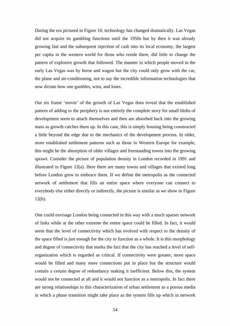
54

During the era pictured in Figure 10, technology has changed dramatically. Las Vegas

did not acquire its gambling functions until the 1950s but by then it was already

growing fast and the subsequent injection of cash into its local economy, the largest

per capita in the western world for those who reside there, did little to change the

pattern of explosive growth that followed. The manner in which people moved in the

early Las Vegas was by horse and wagon but the city could only grow with the car,

the plane and air-conditioning, not to say the incredible information technologies that

now dictate how one gambles, wins, and loses.

Our six frame ‘movie’ of the growth of Las Vegas does reveal that the established

pattern of adding to the periphery is not entirely the complete story for small blobs of

development seem to attach themselves and then are absorbed back into the growing

mass as growth catches them up. In this case, this is simply housing being constructed

a little beyond the edge due to the mechanics of the development process. In older,

more established settlement patterns such as those in Western Europe for example,

this might be the absorption of older villages and freestanding towns into the growing

sprawl. Consider the picture of population density in London recorded in 1991 and

illustrated in Figure 12(a). Here there are many towns and villages that existed long

before London grew to embrace them. If we define the metropolis as the connected

network of settlement that fills an entire space where everyone can connect to

everybody else either directly or indirectly, the picture is similar as we show in Figure

12(b).

One could envisage London being connected in this way with a much sparser network

of links while at the other extreme the entire space could be filled. In fact, it would

seem that the level of connectivity which has evolved with respect to the density of

the space filled is just enough for the city to function as a whole. It is this morphology

and degree of connectivity that marks the fact that the city has reached a level of self-

organization which is regarded as critical. If connectivity were greater, more space

would be filled and many more connections put in place but the structure would

contain a certain degree of redundancy making it inefficient. Below this, the system

would not be connected at all and it would not function as a metropolis. In fact there

are strong relationships to this characterization of urban settlement as a porous media

in which a phase transition might take place as the system fills up which in network

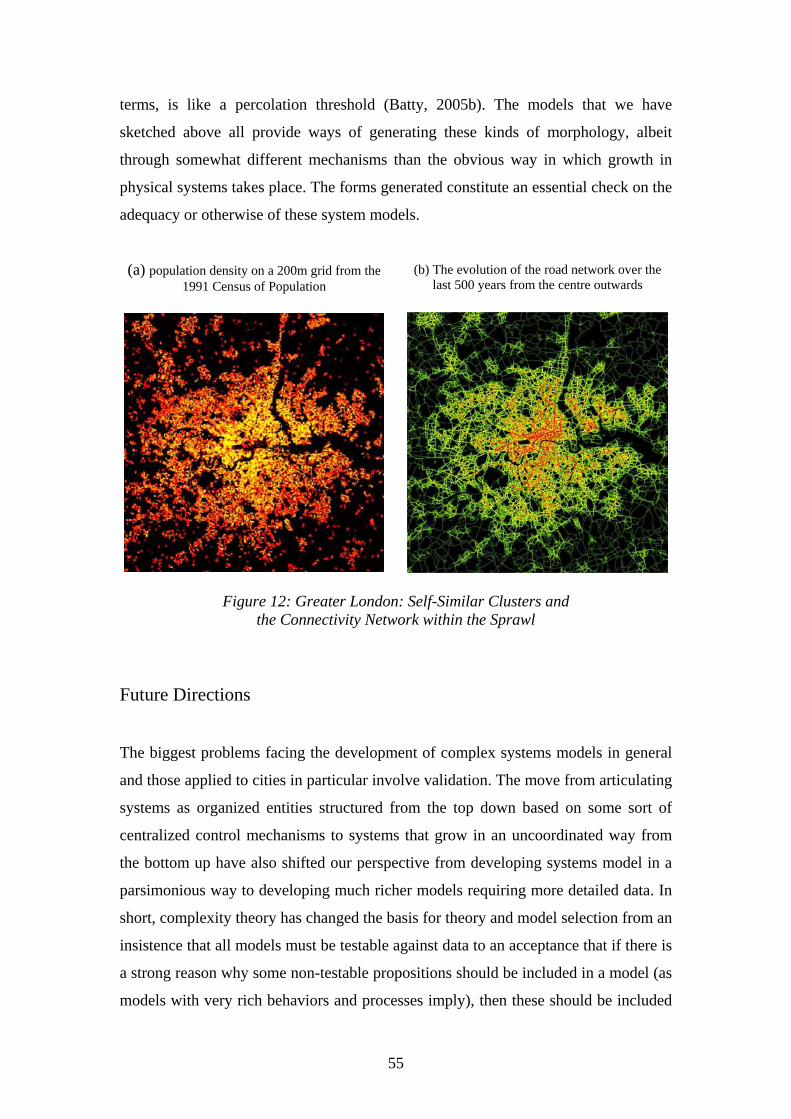
55

terms, is like a percolation threshold (Batty, 2005b). The models that we have

sketched above all provide ways of generating these kinds of morphology, albeit

through somewhat different mechanisms than the obvious way in which growth in

physical systems takes place. The forms generated constitute an essential check on the

adequacy or otherwise of these system models.

(a) population density on a 200m grid from the 1991 Census of Population

(b) The evolution of the road network over the last 500 years from the centre outwards

Figure 12: Greater London: Self-Similar Clusters and the Connectivity Network within the Sprawl

Future Directions

The biggest problems facing the development of complex systems models in general

and those applied to cities in particular involve validation. The move from articulating

systems as organized entities structured from the top down based on some sort of

centralized control mechanisms to systems that grow in an uncoordinated way from

the bottom up have also shifted our perspective from developing systems model in a

parsimonious way to developing much richer models requiring more detailed data. In

short, complexity theory has changed the basis for theory and model selection from an

insistence that all models must be testable against data to an acceptance that if there is

a strong reason why some non-testable propositions should be included in a model (as

models with very rich behaviors and processes imply), then these should be included

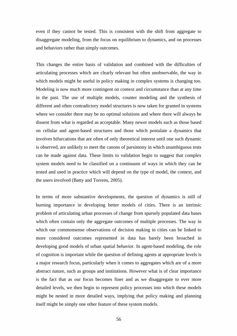
56

even if they cannot be tested. This is consistent with the shift from aggregate to

disaggregate modeling, from the focus on equilibrium to dynamics, and on processes

and behaviors rather than simply outcomes.

This changes the entire basis of validation and combined with the difficulties of

articulating processes which are clearly relevant but often unobservable, the way in

which models might be useful in policy making in complex systems is changing too.

Modeling is now much more contingent on context and circumstance than at any time

in the past. The use of multiple models, counter modeling and the synthesis of

different and often contradictory model structures is now taken for granted in systems

where we consider there may be no optimal solutions and where there will always be

dissent from what is regarded as acceptable. Many newer models such as those based

on cellular and agent-based structures and those which postulate a dynamics that

involves bifurcations that are often of only theoretical interest until one such dynamic

is observed, are unlikely to meet the canons of parsimony in which unambiguous tests

can be made against data. These limits to validation begin to suggest that complex

system models need to be classified on a continuum of ways in which they can be

tested and used in practice which will depend on the type of model, the context, and

the users involved (Batty and Torrens, 2005).

In terms of more substantive developments, the question of dynamics is still of

burning importance in developing better models of cities. There is an intrinsic

problem of articulating urban processes of change from sparsely populated data bases

which often contain only the aggregate outcomes of multiple processes. The way in

which our commonsense observations of decision making in cities can be linked to

more considered outcomes represented in data has barely been broached in

developing good models of urban spatial behavior. In agent-based modeling, the role

of cognition is important while the question of defining agents at appropriate levels is

a major research focus, particularly when it comes to aggregates which are of a more

abstract nature, such as groups and institutions. However what is of clear importance

is the fact that as our focus becomes finer and as we disaggregate to ever more

detailed levels, we then begin to represent policy processes into which these models

might be nested in more detailed ways, implying that policy making and planning

itself might be simply one other feature of these system models.

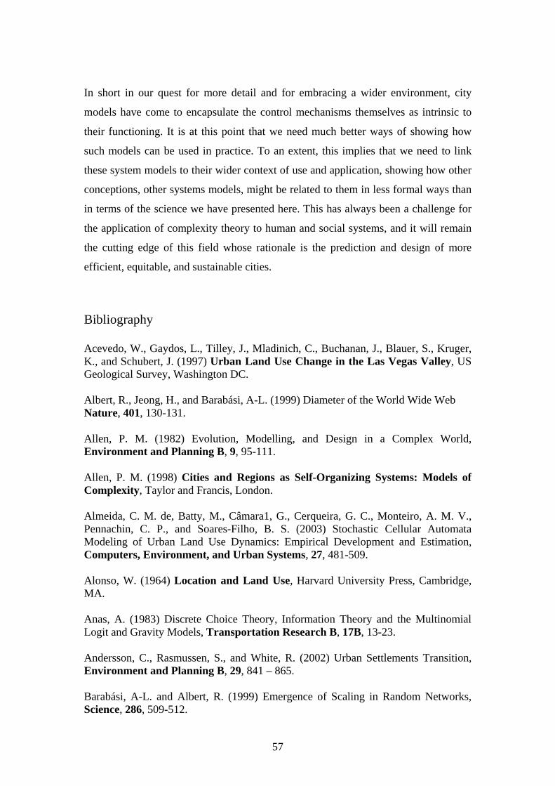
57

In short in our quest for more detail and for embracing a wider environment, city

models have come to encapsulate the control mechanisms themselves as intrinsic to

their functioning. It is at this point that we need much better ways of showing how

such models can be used in practice. To an extent, this implies that we need to link

these system models to their wider context of use and application, showing how other

conceptions, other systems models, might be related to them in less formal ways than

in terms of the science we have presented here. This has always been a challenge for

the application of complexity theory to human and social systems, and it will remain

the cutting edge of this field whose rationale is the prediction and design of more

efficient, equitable, and sustainable cities.

Bibliography Acevedo, W., Gaydos, L., Tilley, J., Mladinich, C., Buchanan, J., Blauer, S., Kruger, K., and Schubert, J. (1997) Urban Land Use Change in the Las Vegas Valley, US Geological Survey, Washington DC. Albert, R., Jeong, H., and Barabási, A-L. (1999) Diameter of the World Wide Web Nature, 401, 130-131. Allen, P. M. (1982) Evolution, Modelling, and Design in a Complex World, Environment and Planning B, 9, 95-111. Allen, P. M. (1998) Cities and Regions as Self-Organizing Systems: Models of Complexity, Taylor and Francis, London. Almeida, C. M. de, Batty, M., Câmara1, G., Cerqueira, G. C., Monteiro, A. M. V., Pennachin, C. P., and Soares-Filho, B. S. (2003) Stochastic Cellular Automata Modeling of Urban Land Use Dynamics: Empirical Development and Estimation, Computers, Environment, and Urban Systems, 27, 481-509. Alonso, W. (1964) Location and Land Use, Harvard University Press, Cambridge, MA. Anas, A. (1983) Discrete Choice Theory, Information Theory and the Multinomial Logit and Gravity Models, Transportation Research B, 17B, 13-23. Andersson, C., Rasmussen, S., and White, R. (2002) Urban Settlements Transition, Environment and Planning B, 29, 841 – 865. Barabási, A-L. and Albert, R. (1999) Emergence of Scaling in Random Networks, Science, 286, 509-512.

58

Barredo, J. I., Kasanko, M., McCormick, N., and Lavalle, C. (2003) Modeling Dynamic Spatial Processes: Simulation of Urban Future Scenarios through Cellular Automata, Landscape and Urban Planning, 64, 145-160. Batty, M. (1974) Spatial Entropy, Geographical Analysis, 6, 1-31. Batty, M. (1976) Urban Modelling: Algorithms, Calibration, Predictions, Cambridge University Press, Cambridge, UK. Batty, M. (2005a) Agents, Cells, and Cities: New Representational Models for Simulating Multiscale Urban Dynamics, Environment and Planning A, 37 (8), 1373-1394. Batty, M. (2005b) Cities and Complexity: Understanding Cities with Cellular Automata, Agent-Based Models, and Fractals, The MIT Press, Cambridge, MA. Batty, M. (2006) Rank Clocks, Nature, 444, 592-596. Batty, M. (2008) The Size, Scale, and Shape of Cities, Science, 319 (5864), 769 – 771. Batty, M. and Longley, P. A. (1994) Fractal Cities: A Geometry of Form and Function, Academic Press, San Diego, CA. Batty, M. and Torrens, P. M. (2005) Modelling and Prediction in a Complex World, Futures, 37 (7), 745-766. Batty, M., and Xie, Y. (1994) From Cells to Cities, Environment and Planning B, 21, s31-s48. Batty, M., Xie, Y., and Sun, Z. (1999) Modeling Urban Dynamics Through GIS-Based Cellular Automata, Computers, Environment and Urban Systems, 23, 205-233. Ben Akiva, M. and Lerman, S. (1985) Discrete Choice Analysis, The MIT Press, Cambridge, MA. Berry, B. J. L. (1964) Cities as Systems within Systems of Cities, Papers and Proceedings of the Regional Science Association, 13, 147–164. Bertalanffy, L. von (1969, 1976) General System Theory: Foundations, Development, Applications, George Braziller, New York, Revised Edition (1976). Besussi, E., Cecchini, A., and Rinaldi, E. (1998) The Diffused City of the Italian North-East: Identification of Urban Dynamics Using Cellular Automata Urban Models, Computers, Environment and Urban Systems, 22, 497-523. Blank, A. and Solomon, S. (2000) Power Laws in Cities Population, Financial Markets and Internet Sites: Scaling and Systems with a Variable Number of Components, Physica A, 287, 279-288.

59

Cardillo, A., Scellato, S., Latora, V., Porta, S., (2006) Structural Properties of Planar Graphs of Urban Street Patterns, Physical Review E, 73, 066107-1- to 8 Castle, C. J. E. and Crooks, A. T. (2006) Principles and Concepts of Agent-Based Modelling for Developing Geospatial Simulations, Working Paper 110, Centre for Advanced Spatial Analysis, University College London, London. Chadwick, G. F. (1971) A Systems View of Planning, Pergamon Press, Oxford, UK. Chapin, F. S. and Weiss, S. F. (1968) A Probabilistic Model for Residential Growth, Transportation Research, 2, 375-390. Cheng, J. (2003) Modelling Spatial and Temporal Urban Growth, PhD Thesis, ITC Dissertation 99, ITC, Enschede, The Netherlands. Clark, C. (1951) Urban Population Densities, Journal of the Royal Statistical Society, Series A, 114, 490-496. Clarke, G. (Editor) (1996) Microsimulation for Urban and Regional Policy Analysis, Pion Press, London. Clarke, K. C., and Gaydos, L. J. (1998) Loose Coupling a Cellular Automaton Model and GIS: Long-Term Growth Prediction for San Francisco and Washington/Baltimore, International Journal of Geographical Information Science, 12, 699-714. Couclelis, H. (1985) Cellular Worlds: A Framework for Modeling Micro-Macro Dynamics, Environment and Planning A, 17, 585-596. Crucitti, P., Latora, V., and Porta, S. (2006) Centrality Measures in Spatial Networks of Urban Streets, Physical Review E, 73, 036125-1-5. Curry, L. (1964) The Random Spatial Economy: An Exploration in Settlement Theory, Annals of the Association of American Geographers, 54, 138-146. Dendrinos, D. S., and Mullally, H. (1985) Urban Evolution: Studies in the Mathematical Ecology of Cities, Oxford University Press, Oxford, UK. Epstein, J. M. and Axtell, R. L. (1996) Growing Artificial Societies: Social Science from the Bottom Up, The MIT Press, Cambridge, MA. Feigenbaum, M. J. (1980) The Metric Universal Properties of Period Doubling Bifurcations and the Spectrum for a Route to Turbulence, Annals of the New York Academy of Sciences, 357, 330-336. Forrester, J. W. (1969) Urban Dynamics, The MIT Press, Cambridge, MA. Fujita, M., Krugman, P., and Venables, A. J. (1999) The Spatial Economy: Cities, Regions, and International Trade, The MIT Press, Cambridge, MA.

60

Gabaix, X. (1999) Zipf's Law for Cities: An Explanation, Quarterly Journal of Economics, 114, 739-767. Gell-Man, M. (1994) The Quark and the Jaguar: Adventures in the Simple and the Complex, W. H. Freeman and Company, New York. Gibrat, R. (1931) Les Inégalités Économiques, Librarie du Recueil Sirey, Paris. Gilbert, N. (2007) Agent-Based Models, Sage Inc., Thousand Oaks, CA. Haag, G. (1989) Dynamic Decision Theory: Applications to Urban and Regional Topics, Kluwer, Dordrecht, The Netherlands. Helbing, D. and Nagel, K. (2004) The Physics of Traffic and Regional Development, Contemporary Physics, 45, 405-426. Hillier, B. (1996) Space is the Machine, Cambridge University Press, Cambridge, UK. Jiang, B. (2007) A Topological Pattern of Urban Street Networks: Universality and Peculiarity, Physica A, 384, 647-655. Lathrop, G. T., and Hamburg, J. R. (1965) An Opportunity-Accessibility Model for Allocating Regional Growth, Journal of the American Institute of Planners, 31, 95-103. Lowry, I. S. (1964) Model of Metropolis, Memorandum RM-4035-RC, Rand Corporation, Santa Monica, CA. Mandelbot, B. B. (1983) The Fractal Geometry of Nature, W. H. Freeman, New York. May, R. M. (1976) Simple Mathematical Models with Very Complicated Dynamics, Nature, 261, 459–467. McLoughlin, J. B. (1969) Urban and Regional Planning: A Systems Approach, Faber and Faber, London. Miller, J. H. and Page, S. E. (2007) Complex Adaptive Systems: An Introduction to Computational Models of Social Life, Princeton University Press, Princeton, NJ. Nagel, K., Beckman, R.J. and Barrett, C.L. (1999) TRANSIMS for Urban Planning, LA-UR 984389, Los Alamos National Laboratory, Los Alamos, NM. Newman, M., Barabási, A-L., and Watts, D. J. (2006) The Structure and Dynamics of Networks, Princeton University Press, Princeton, NJ. Nijkamp, P., and Reggiani, A. (1992) Interaction, Evolution and Chaos in Space, Springer Verlag, Berlin, DE.

61

Papini, L. Rabino, G. A., Colonna, A., Di Stefano, V., and Lombardo, S. (1998) Learning Cellular Automata in a Real World: The Case Study of the Rome Metropolitan Area, in S. Bandini, R. Serra, and F. Suggi Liverani (Editors) Cellular Automata: Research Towards Industry: ACRI’96, Proceedings of the Third Conference on Cellular Automata for Research and Industry, Springer-Verlag, London, 165-183. Portugali, J., and Benenson, I. (1996) Human Agents between Local and Global Forces in a Self-Organizing City, in F. Schweitzer (Editor) Self-Organization of Complex Structures: From Individual to Collective Dynamics, Gordon and Breach, London, 537-545. Propolis (2004) PROPOLIS (Policies and Research of Policies for Land Use and Transport for Increasing Urban Sustainability), Final Report for the Commission of the European Communities, LT Consultants Ltd., Helsinki, Finland. Sanders, L., Pumain, D., Mathian, H., Guerin-Pace, F., and Bura, S. (1997) SIMPOP: A Multiagent System for the Study of Urbanism, Environment and Planning B, 24, 287-305. Schelling, T. C. (1969) Models of Segregation, American Economic Review, Papers and Proceedings, 58 (2), 488-493. Schelling, T. C. (1978) Micromotives and Macrobehavior, W. W. Norton and Company, New York. Schweitzer, F. and Steinbrink, J. (1997) Urban Cluster Growth: Analysis and Computer Simulation of Urban Aggregations, in F. Schweitzer (Editor) Self-Organization of Complex Structures: From Individual to Collective Dynamics, Gordon and Breach, London, 501-518. Semboloni, F. (2000) The Growth of an Urban Cluster into a Dynamic Self-Modifying Spatial Pattern, Environment and Planning B, 27, 549 – 564. Thünen, J.H. von (1826, 1966) Von Thunen’s Isolated State (1966 translation from the 1826 German Edition Der Isolierte Staat in Beziehung auf Landwirtschaft und Nationaloekonomie by P. G. Hall), Pergamon, Oxford, UK. Tobler, W. R. (1970) A Computer Movie Simulating Population Growth in the Detroit Region, Economic Geography, 42, 234-240. Tribus, M. (1969) Rational, Descriptions, Decisions and Designs, Pergamon Press, New York. Waddell, P. (2002) UrbanSim: Modeling Urban Development for Land Use, Transportation and Environmental Planning, Journal of the American Planning Association, 68, 297-314.

62

Ward, D. P., Murray, A. T., and Phinn, S. R. (2000) A Stochastically Constrained Cellular Model of Urban Growth, Computers, Environment and Urban Systems, 24, 539-558. Wegener, M. (2005) Urban Land-Use Transportation Models, in D. J. Maguire, M. Batty, and M. F. Goodchild (Editors) (2005) GIS, Spatial Analysis, and Modeling, ESRI Press, Redlands, CA, pp. 203-220. White, R. W., and Engelen, G. (1993) Cellular Automata and Fractal Urban Form: A Cellular Modelling Approach to the Evolution of Urban Land Use Patterns, Environment and Planning A, 25, 1175-1193. Wiener, N. (1948, 1965) Cybernetics: or the Control and Communication in the Animal and the Machine, The MIT Press, Cambridge, MA, Second Edition, 1965. Wilson, A. G. (1970) Entropy in Urban and Regional Modelling, Pion Press, London. Wilson, A. G. (1981) Catastrophe Theory and Bifurcation; Applications to Urban and Regional Systems, University of California Press, Berkeley, CA. Wilson, A. G. (2007) Boltzmann, Lotka, and Volterra and Spatial Structural Evolution: A Integrated Methodology for Some Dynamical Systems, Journal of the Royal Society Interface, doi:10.1098/rsif.2007.1288, 1-7. Wu, F., and Webster, C. J. (1998) Simulation of Land Development through the Integration of Cellular Automata and Multicriteria Evaluation, Environment and Planning B, 25, 103-126. Xie, Y. (1994) Analytical Models and Algorithms for Cellular Urban Dynamics, unpublished PhD dissertation, State University of New York at Buffalo, Buffalo, NY. Xie, Y., and Batty, M. (2005) Integrated Urban Evolutionary Modeling, in P. M. Atkinson, G. M. Foody, S. E. Darby, and F. Wu (Editors) Geodynamics, CRC Press, Boca Raton, FL, 273-293. Yeh, A. G-O., and Li., X. (2000) A ‘Grey-Cell’ Constrained CA Model for the Simulation of Urban Forms and Developments in the Planning of Sustainable Cities using GIS, Centre of Urban Planning and Environmental Management, University of Hong Kong, Pokfulam, Hong Kong. Zipf, G. K. (1949) Human Behavior and the Principle of Least Effort, Addison-Wesley, Cambridge, MA.

Documents

Cities as complex systems: scaling, interactions, networks, dynamics and urban morphologies