Embed Size (px)
Citation preview

Hauerhof, E. (2017). The assessment of oil products tanker design methods and technologies to
enhance the Energy Efficiency Design Index measure by means of computer simulation and trend
analysis. (Unpublished Doctoral thesis, City, University of London)
City Research Online
Original citation: Hauerhof, E. (2017). The assessment of oil products tanker design methods and
technologies to enhance the Energy Efficiency Design Index measure by means of computer
simulation and trend analysis. (Unpublished Doctoral thesis, City, University of London)
Permanent City Research Online URL: http://openaccess.city.ac.uk/17635/
Copyright & reuse
City University London has developed City Research Online so that its users may access the
research outputs of City University London's staff. Copyright © and Moral Rights for this paper are
retained by the individual author(s) and/ or other copyright holders. All material in City Research
Online is checked for eligibility for copyright before being made available in the live archive. URLs
from City Research Online may be freely distributed and linked to from other web pages.
Versions of research
The version in City Research Online may differ from the final published version. Users are advised
to check the Permanent City Research Online URL above for the status of the paper.
Enquiries
If you have any enquiries about any aspect of City Research Online, or if you wish to make contact
with the author(s) of this paper, please email the team at [email protected].
The assessment of oil products tanker
design methods and technologies to enhance
the Energy Efficiency Design Index measure
by means of
computer simulation and trend analysis
Elena Hauerhof
This thesis is submitted for the degree of
Doctor of Philosophy
Department of Mechanical Engineering and Aeronautics
City University London
Supervisors
Professor John Carlton, FREng
Professor Dinos Arcoumanis, FREng
School of Mathematics, Computer Science and Engineering
May 2017
2
Table of Contents
Table of Contents ................................................................................................................. 2
List of Figures ...................................................................................................................... 4
List of Tables ..................................................................................................................... 11
Acknowledgments ............................................................................................................. 14
Abstract .............................................................................................................................. 15
Abbreviations and Explanatory Notes ............................................................................... 16
General Nomenclature ....................................................................................................... 19
EEDI Nomenclature ........................................................................................................... 23
1 Introduction ..................................................................................................................... 24
2 Ship as a System Approach: Methods and Technologies to Enhance Ship Energy Efficiency ........................................................................................................................... 45
2.1 Operational Strategies .............................................................................................. 50
2.2 Hull Optimisation .................................................................................................... 56
2.3 Propellers and Energy Saving Devices .................................................................... 60
2.4 Machinery Improvements ........................................................................................ 67
2.5 Alternative Ship Propulsion and Fuels .................................................................... 75
3 Challenges in EEDI formulation .................................................................................... 92
4 The Reference Ship: Oil Products Tanker ...................................................................... 94
4.1 PhD Research Structure ........................................................................................... 97
5 Ship Performance Simulation Model .............................................................................. 99
5.1 Module 1: Resistance and Propulsion .................................................................... 100
5.2 Module 2: Engine Performance Simulation .......................................................... 113
5.3 Module 3: Exhaust Emissions Prediction Model ................................................... 117
5.4 Module 4: Energy Efficiency Design Index (EEDI) Calculator ............................ 143
6 Time Domain Voyage Simulation ................................................................................ 144
7 Energy Efficient Propellers ........................................................................................... 154
7.1 The Effect of a Wake Equalising Duct .................................................................. 155
7.2 CLT Propellers ....................................................................................................... 164
7.3 Ducted Propellers ................................................................................................... 169
3
7.4 Impact on the Energy Efficiency Indicators .......................................................... 176
8 Propeller Optimisation .................................................................................................. 181
8.1 The Effect of BAR on Ship Efficiency .................................................................. 183
8.2 The Effect of Artificially Increased Propeller Diameters ...................................... 188
8.3 Impact on the Energy Efficiency Indicators .......................................................... 196
9 Maximum Propeller Diameter ...................................................................................... 203
9.1 The Estimation of the Optimum Diameter-RPM Combinations ........................... 203
9.2 Propeller Clearances .............................................................................................. 206
9.3 Propellers Performance Analysis ........................................................................... 208
9.4 Impact on the Energy Efficiency Indicators .......................................................... 214
10 Energy Efficient Trim Optimisation ........................................................................... 220
10.1 Trim Definition .................................................................................................... 221
10.2 Hull Design Parameters ....................................................................................... 223
10.3 Ship Resistance .................................................................................................... 223
10.4 Propulsive Efficiency ........................................................................................... 227
10.5 Impact on the Energy Efficiency Indicators ........................................................ 229
11 Future Hybrid Propulsion Concepts ............................................................................ 233
11.1 On-Time Voyage Simulation ............................................................................... 235
11.2 Optimum Load Voyage Simulation ..................................................................... 240
12 EEDI Amendments Proposal ...................................................................................... 246
13 Conclusion .................................................................................................................. 258
14 Recommendations ....................................................................................................... 265
15 Suggestions for Further Research ............................................................................... 266
References ........................................................................................................................ 267
Appendix I. The Energy Efficiency Design Index Methodology .................................... 273
Appendix II. Propeller Design Procedure for Wageningen series ................................... 282
Appendix III. Blade Area Ratio Estimation Procedure.................................................... 287
4
List of Figures
Figure 1.1 Growth of international seaborne trade over selected years. ......................................... 24
Figure 1.2. World seaborne trade in cargo ton–miles by cargo type. ............................................. 25
Figure 1.3 World fleet by vessel type. ............................................................................................ 25
Figure 1.4 Percentage distribution of the world fleet by ship category in 2015. ............................ 26
Figure 1.5 Simplified composition of the exhaust gas flow from the ship with 2-stroke diesel engine burning the ISO 8217 fuel oil. ........................................................................................................ 27
Figure 1.6 The total shipping 𝐶𝐶𝐶𝐶2 emissions for the period 2007-2012......................................... 28
Figure 1.7 The 𝑁𝑁𝐶𝐶𝑋𝑋 emissions for the period of 2007 – 2012 in million tonnes of 𝑁𝑁𝐶𝐶2. .............. 29
Figure 1.8 The 𝑆𝑆𝐶𝐶𝑋𝑋 emissions for the period of 2007 – 2012 in million tonnes of 𝑆𝑆𝐶𝐶2. ................ 30
Figure 1.9 The 𝐶𝐶𝐶𝐶 emissions in million tonnes from shipping industry for the period of 2007-2012. ........................................................................................................................................................ 31
Figure 1.10 The 𝑁𝑁𝑁𝑁𝑁𝑁𝐶𝐶𝐶𝐶 emissions in million tonnes from shipping industry for the period of 2007-2012. ............................................................................................................................................... 32
Figure 1.11 The 𝑃𝑃𝑁𝑁 emissions in million tonnes from shipping industry for the period of 2007-2012. ............................................................................................................................................... 33
Figure 1.12 The overall impact of the atmospheric emissions from shipping on the environment. ........................................................................................................................................................ 35
Figure 1.13 Top 10 Flags of registration with the largest registered fleets as of 1 January 2015... 37
Figure 1.14 Ownership of the world fleet as of 1 January 2015 ..................................................... 37
Figure 1.15 Main components of the legislative framework of the shipping industry ................... 39
Figure 1.16 IMO air pollution prevention legislative framework ................................................... 40
Figure 2.1 Integrated ship system diagram ..................................................................................... 49
Figure 2.2 Average at-sea main engine load factor for oil tankers in 2007 - 2012 ......................... 51
Figure 2.3 Oil tankers: percentage change in fuel consumption associated with the 1 percent reduction in steel weight ................................................................................................................. 57
Figure 2.4 SFOC behaviour comparison under conventional and de-rated conditions. ................. 70
Figure 2.5 Average daily fuel oil consumption. Based on annual BP review ................................ 76
Figure 2.6 General range of biofuels types and their production routes. ........................................ 79
Figure 2.7 Aquarius MRE (Marine Renewable Energy) system by Eco Marine Power. ............... 83
Figure 2.8 Steam turbine plant powered by a nuclear reactor ........................................................ 85
Figure 2.9 Working principle of the basic solid polymer fuel cell ................................................. 87
Figure 2.10 Battery based load leveling ship operation concept .................................................... 91
Figure 4.1 World seaborne trade of petroleum products and gas in million of tonnes ................... 94
Figure 4.2 Global tankers fleet distribution .................................................................................... 95
5
Figure 5.1 Ship Performance Simulation (SPS) model .................................................................. 99
Figure 5.2 General components of ship’s total resistance ............................................................ 101
Figure 5.3 The workflow of the ship resistance and propulsion prediction module..................... 105
Figure 5.4 The comparison chart of the effective power from the model test report (MTR) and effective power obtained from the H&M regression-based simulation of the naked hull under the design load condition .................................................................................................................... 107
Figure 5.5 The comparison chart of the effective power from the model test report (MTR) and effective power obtained from the H&M regression-based simulation of the naked hull under the ballast condition............................................................................................................................ 107
Figure 5.6 Comparison diagram of the open water test (OWT) data from the model test report (MTR) and computations using the Wageningen B-screw series (WAG) regression-based method ...................................................................................................................................................... 110
Figure 5.7 The energy flow diagram of the conventional mechanical drive system installed on the reference tanker. ........................................................................................................................... 113
Figure 5.8 The resulting table of the CEAS engine simulation tool ............................................. 116
Figure 5.9 The 5S50ME-C engine layout and performance diagram ........................................... 116
Figure 5.10 𝐶𝐶𝐶𝐶 and 𝐻𝐻𝐶𝐶 spline interpolation results ..................................................................... 119
Figure 5.11 The absolute humidity of intake air 𝐻𝐻𝐻𝐻 spline interpolation validation ................... 120
Figure 5.12 Comparison pattern of the absolute humidity of the intake air and dry/wet correction factors over range of engine loads ................................................................................................ 121
Figure 5.13 Comparison pattern of the exhaust gas flow and dry/wet correction factors over range of engine loads .............................................................................................................................. 121
Figure 5.14 The comparison plot of the 𝐶𝐶𝐶𝐶2 concentrations in dry exhaust ................................ 127
Figure 5.15 The comparison analysis of the dry 𝐶𝐶2 concentrations calculated using the reversed fuel analysis procedure and the dry 𝐶𝐶2 concentrations listed in the 𝑁𝑁𝐶𝐶𝑋𝑋 technical file of 7S50MC-C ...................................................................................................................................................... 134
Figure 5.16 Expanded initial 𝑁𝑁𝐶𝐶𝑋𝑋 dataset based on cubic spline interpolation ........................... 137
Figure 5.17 The validation of 𝑁𝑁𝐶𝐶𝑋𝑋 model output for 7S50MC-C engine: the 𝑁𝑁𝐶𝐶𝑋𝑋 technical file based interpolated volumetric 𝑁𝑁𝐶𝐶𝑋𝑋 concentrations vs. the 𝑁𝑁𝐶𝐶𝑋𝑋 model output ............................ 138
Figure 5.18 Resulted 𝑁𝑁𝐶𝐶𝑋𝑋 concentrations of 5S50MC-C engine compared to initial 𝑁𝑁𝐶𝐶𝑋𝑋 concentrations of 7S50MC-C engine ........................................................................................... 138
Figure 5.19 The comparison of exhaust gas temperatures of 7S50MC-C and 5S50ME-C engines ...................................................................................................................................................... 139
Figure 5.20 Attained and required EEDIs for the reference oil products tanker .......................... 143
Figure 6.1 Typical service data relationships (Molland et al. 2011) ............................................ 145
Figure 6.2. The effect of weather on ship’s power requirements based on the trial allowances simulation model .......................................................................................................................... 147
Figure 6.3 Unfiltered Admiralty coefficient versus apparent slip ................................................ 148
6
Figure 6.4 Filtered Admiralty coefficient versus apparent slip .................................................... 149
Figure 6.5 Filtered service data in time domain. Numbers at the top of the graph are Beaufort numbers ......................................................................................................................................... 149
Figure 6.6 Filtered service data with engine power corrected to the mean displacement............. 150
Figure 6.7 Filtered service data sorted by Beaufort number and speed ........................................ 150
Figure 6.8 Artificial time-domain ship performance simulation. Numbers at the top of the graph are Beaufort numbers .......................................................................................................................... 151
Figure 6.9 Artificial ship performance in service sorted by Beaufort number, speed and load condition. Numbers at the top of the graph are Beaufort numbers ............................................... 152
Figure 6.10 The reference ship time-domain voyage simulation. Numbers at the top of the graph are Beaufort numbers .................................................................................................................... 153
Figure 7.1 Current propulsion system of the reference products tanker fitted with a CLT propeller ...................................................................................................................................................... 154
Figure 7.2 Effective power comparison between the propulsion systems with and without the wake equalizing duct. ............................................................................................................................. 157
Figure 7.3 The open water efficiency correction to the Wageningen standards. .......................... 158
Figure 7.4 The wake fraction comparison results of the fixed pitch propeller with the wake equalizing duct (FPP_WED) based on the model test report versus the conventional fixed pitch propeller (FPP) calculated using the Holtrop and Mennen approach ........................................... 159
Figure 7.5 The thrust deduction comparison results of the fixed pitch propeller with the wake equalizing duct (FPP_WED) based on the model test report versus the conventional fixed pitch propeller (FPP) calculated using the Holtrop and Mennen approach ........................................... 160
Figure 7.6 The hull efficiency comparison results of the fixed pitch propeller with the wake equalizing duct (FPP_WED) based on the model test report versus the conventional fixed pitch propeller (FPP) calculated using the Holtrop and Mennen approach ........................................... 161
Figure 7.7 The open water efficiency comparison results of the fixed pitch propeller with the wake equalizing duct (FPP_WED) based on the model test report and corrected to the Wageningen standards versus the conventional fixed pitch propeller (FPP) calculated using the Holtrop and Mennen approach .......................................................................................................................... 162
Figure 7.8 The QPC comparison results of the fixed pitch propeller with the wake equalizing duct (FPP_WED) based on the model test report and corrected to the Wageningen standards versus the conventional fixed pitch propeller (FPP) calculated using the Holtrop and Mennen approach ... 162
Figure 7.9 The power absorption requirements of the fixed pitch propeller with the wake equalizing duct (FPP_WED) based on the model test report and corrected to the Wageningen standards versus the conventional fixed pitch propeller (FPP) calculated using the Holtrop and Mennen approach ...................................................................................................................................................... 163
Figure 7.10 The full-scale CLT propeller and the conventional fixed pitch (FP) propeller curves ...................................................................................................................................................... 166
Figure 7.11 The wake fraction comparison results of the fixed pitch propeller (FPP_WED) and the CLT propeller (CLT_WED) both with the wake equalising duct ................................................ 166
7
Figure 7.12 The hull efficiency comparison results of the fixed pitch propeller (FPP_WED) and the CLT propeller (CLT_WED) both with the wake equalising duct ................................................ 167
Figure 7.13 The open water efficiency comparison results of the fixed pitch propeller (FPP_WED) and the CLT propeller (CLT_WED) both with the wake equalising duct .................................... 168
Figure 7.14 The power absorption results of the fixed pitch propeller (FPP_WED) and the CLT propeller (CLT_WED) both with the wake equalising duct ......................................................... 168
Figure 7.15 The Ka 4-70 propeller diameter interpolation diagram as part of the propeller design procedure ...................................................................................................................................... 171
Figure 7.16. Ducted propeller design procedure .......................................................................... 172
Figure 7.17 The comparison results of the hull efficiency of the 19A ducted propeller (DUCT) and the conventional fixed pitch propeller (FPP) ................................................................................ 173
Figure 7.18 The comparison results of the propeller efficiency of the 19A ducted propeller (DUCT) and the conventional fixed pitch propeller ................................................................................... 174
Figure 7.19 The comparison results of the propulsive efficiency (QPC) of the 19A ducted propeller (DUCT) and the conventional fixed pitch propeller (FPP) .......................................................... 175
Figure 7.20 The power absorption of the 19A ducted propeller system (DUCT) and the conventional fixed pitch propeller (FPP) ........................................................................................................... 175
Figure 7.21 The comparative analysis of the required delivered power under different loads and corresponding operational speed .................................................................................................. 176
Figure 7.22 Engines service curves for all the propeller systems ................................................. 177
Figure 7.23 The EEDI results for all propeller systems ............................................................... 179
Figure 7.24 The voyage simulation results of all propeller systems ............................................ 180
Figure 8.1 Effect of 𝐵𝐵𝐵𝐵𝐵𝐵 on the relative-rotative efficiency 𝜂𝜂𝑅𝑅 .................................................. 184
Figure 8.2 Effect of 𝐵𝐵𝐵𝐵𝐵𝐵s on the open water efficiency for the 4-bladed propeller .................... 185
Figure 8.3 Effect 𝐵𝐵𝐵𝐵𝐵𝐵s on ship delivered power 𝑃𝑃𝐷𝐷 over a range of speeds. .............................. 186
Figure 8.4 Artificial 𝐵𝐵𝐵𝐵𝐵𝐵 cavitation performance based on Burrill’s curves .............................. 186
Figure 8.5 Power absorption of the conventional fixed pitch propeller with the original 𝐵𝐵𝐵𝐵𝐵𝐵 = 0.5628 vs 𝐵𝐵𝐵𝐵𝐵𝐵 = 0.4 under design, ballast and loaded conditions ............................................... 188
Figure 8.6 Thrust loading distribution for the artificial propeller diameters ................................ 189
Figure 8.7 Propeller design process based on the artificially selected propeller diameters ......... 190
Figure 8.8 Hull efficiency behaviour with the artificially changing propeller diameters ............. 191
Figure 8.9 Relative-rotative efficiency behaviour with changing propeller diameters ................ 192
Figure 8.10 Open water efficiency behaviour with changing propeller diameters ....................... 193
Figure 8.11 Effect of the artificially increased propeller diameters on ship delivered power 𝑃𝑃𝐷𝐷 over a range of speeds. ......................................................................................................................... 193
Figure 8.12 Cavitation performance due to the artificial diameters based on Burrill’s curves .... 194
8
Figure 8.13 Comparison plot of the power absorption requirements of the fixed pitch propeller with the original 𝐷𝐷 = 5.65m and the artificially increased and decreased diameters by 5 percent under design, ballast and loaded conditions............................................................................................ 196
Figure 8.14 Comparative analysis of the required delivered power under different loads and corresponding operational speed................................................................................................... 197
Figure 8.15 Engines service curves for FPP_ORG, FPP_BAR_MIN, FPP_D_PLUS_5% propeller systems. ......................................................................................................................................... 198
Figure 8.16 Enlarged version of Figure 8.15. Engines service curves for FPP_ORG, FPP_BAR_MIN, FPP_D_PLUS_5% propeller systems. ............................................................. 198
Figure 8.17 EEDI results for FPP_ORG, FPP_BAR_MIN, FPP_D_PLUS_5% propeller systems. ...................................................................................................................................................... 200
Figure 8.18 Voyage simulation results for FPP_ORG, FPP_BAR_MIN, FPP_D_PLUS_5% propeller systems. ......................................................................................................................... 200
Figure 9.1 Optimum RPM – diameter range design process ........................................................ 205
Figure 9.2 Resulted optimum RPM – diameter range .................................................................. 206
Figure 9.3 Hull surface pressure distribution ................................................................................ 206
Figure 9.4 FPP_MAX (left) and FPP_MAX_SHAFT (right) applied to the reference stern design with the lifted shaft on the latter case. .......................................................................................... 207
Figure 9.5 𝐵𝐵𝑃𝑃𝑁𝑁 – diameter ranges at different ship speeds (design conditions) .......................... 209
Figure 9.6 Resulted 𝐵𝐵𝑃𝑃𝑁𝑁 distributions at different loads............................................................. 210
Figure 9.7 Hull efficiency results for FPP, FPP_MAX and FPP_MAX_SHAFT at the ballast, design and loaded conditions. .................................................................................................................. 211
Figure 9.8 Relative-rotative efficiency results for FPP, FPP_MAX and FPP_MAX_SHAFT at the ballast, design and loaded conditions............................................................................................ 212
Figure 9.9 Open water efficiency results for FPP, FPP_MAX and FPP_MAX_SHAFT at the ballast, design and loaded conditions. ....................................................................................................... 212
Figure 9.10 Delivered power results for FPP, FPP_MAX and FPP_MAX_SHAFT at the ballast, design and loaded conditions. ....................................................................................................... 213
Figure 9.11 Hull surface pressures for FPP, FPP_MAX and FPP_MAX_SHAFT at the ballast, design and loaded conditions. ....................................................................................................... 213
Figure 9.12 Engines service curves for all propeller systems ....................................................... 215
Figure 9.13 EEDI results for all propeller systems. ...................................................................... 217
Figure 9.14 Voyage simulation results of all propeller systems. .................................................. 218
Figure 10.1 Schematic representation of considered trim conditions. .......................................... 221
Figure 10.2 Frictional resistance 𝐵𝐵𝐹𝐹 and frictional coefficient 𝐶𝐶𝐹𝐹 performance due to changing trim. ...................................................................................................................................................... 224
Figure 10.3 Bulbous bow resistance 𝐵𝐵𝐵𝐵𝐵𝐵 and correlation resistance 𝐵𝐵𝐴𝐴 performance due to changing trim. ............................................................................................................................................... 225
9
Figure 10.4 Wave-making resistance 𝐵𝐵𝑊𝑊 performance due to changing trim. ............................. 225
Figure 10.5 Total resistance 𝐵𝐵𝑇𝑇 and effective power 𝑃𝑃𝐸𝐸 performance due to changing trim. ...... 226
Figure 10.6 Effect on the propulsive efficiency components due to changing trim. .................... 228
Figure 10.7 Power absorption 𝐵𝐵𝐷𝐷 and 𝑄𝑄𝑃𝑃𝐶𝐶 performance due to changing trim. ......................... 228
Figure 10.8 Resulting level of gains and reductions of power in percentage due to changing trim ...................................................................................................................................................... 229
Figure 10.9 Engines service curves for partially loaded operation at both trim conditions and the even keel ....................................................................................................................................... 230
Figure 10.10 Voyage simulation results for both trim conditions and the even keel. Numbers at the top of the graph are Beaufort numbers ......................................................................................... 231
Figure 11.1 Original voyage of the reference oil products tanker. Numbers at the top of the graph are rotational speeds ..................................................................................................................... 234
Figure 11.2 Hybrid-based machinery arrangement for the reference vessel ............................... 234
Figure 11.3 Ship speed distribution during the original voyage ................................................... 236
Figure 11.4 Sea state probability analysis results ......................................................................... 236
Figure 11.5 Speed, load and SFOC arrangements for the completed voyage on time (ON_TIME) operation ....................................................................................................................................... 237
Figure 11.6 ON_TIME voyage simulation. Numbers at the top of the graph are Beaufort numbers ...................................................................................................................................................... 237
Figure 11.7 ON_TIME battery charging/discharging diagram .................................................... 238
Figure 11.8 ON_TIME_SPEED voyage simulation ..................................................................... 239
Figure 11.9 ON_TIME_SPEED battery charging/discharging diagram ...................................... 239
Figure 11.10 Speed, load and SFOC arrangements for the OPTIMUM operation ...................... 241
Figure 11.11 OPTIMUM voyage simulation ............................................................................... 242
Figure 11.12 OPTIMUM battery charging/discharging diagram ................................................. 242
Figure 11.13 OPTIMUM_SPEED voyage simulation ................................................................. 243
Figure 11.14 OPTIMUM_SPEED battery charging/discharging diagram ................................... 243
Figure 12.1 Attained EEDI, required EEDI due to 2015 and the EEDI weather of the reference oil products tanker ............................................................................................................................. 247
Figure 12.2 Measured ship service engine power and ship speed observed................................. 248
Figure 12.3 Service data used for the EEDI calculation: service SMCR, original engine power measurements and SFOC at 75 percent load corresponding to service SMCR. ........................... 249
Figure 12.4 Service data used for the EEDI calculation: ship DWT and speed observed. ........... 250
Figure 12.5 Resulting service EEDI distribution sorted by Beaufort number. ............................. 250
Figure 12.6 Mean service EEDI indexes grouped by Beaufort number in comparison with the original attained EEDI, reference EEDI and the EEDI weather. .................................................. 251

10
Figure 12.7 The effect of weather on service engine power and ship speed behaviour............... 251
Figure 12.8 Mean service DWT, mean service speeds and their linear trend lines. ..................... 252
Figure 12.9 3D map correlation between the Beaufort scale, ship displacement and the EEDI measure ......................................................................................................................................... 253
Figure 12.10 Mean service EEDI indexes based on constant DWT grouped by Beaufort number in comparison with the original attained EEDI, reference EEDI and the EEDI weather. ................. 254
Figure 12.11 Resulting constant DWT EEDI distribution sorted by Beaufort number in comparison with the originally obtained service DWT. ................................................................................... 254
Figure 12.12 Sea state probability analysis results ....................................................................... 255
Figure 12.13 Original attained EEDI, EEDI weather and the amended EEDI values .................. 256
11
List of Tables Table 2.1 Potential applicability and implementation time frame of energy efficient measures and technologies ................................................................................................................................ 47
Table 2.2 General properties of hull coatings prevailed in service ............................................ 55
Table 2.3 Maximum allowable ship dimensions in canals and channels ................................... 58
Table 2.4 Recommended WHRS for various propulsion systems based on the rule of thumb .. 74
Table 2.5 Li-ion cell comparison ................................................................................................ 89
Table 4.1 Basic propellers characteristics .................................................................................. 95
Table 4.2 Principle ship dimensions based on model test report ................................................ 96
Table 5.1 Complete resistance and propulsion module simulation results for designed, ballast and loaded conditions ...................................................................................................................... 111
Table 5.2 The 𝑁𝑁𝐶𝐶𝑋𝑋file emissions data related to the 7S50MC-C marine diesel engine .......... 117
Table 5.3 The elemental chemical breakdown of the MDO fuel used ..................................... 118
Table 5.4 Coefficient 𝑢𝑢𝑔𝑔𝑔𝑔𝑔𝑔 for raw exhaust gas ....................................................................... 122
Table 5.5 𝐶𝐶𝐶𝐶 calculation results for the reference engine 5S50ME-C ..................................... 123
Table 5.6 𝐻𝐻𝐶𝐶 calculation results for the reference engine 5S50ME-C ..................................... 124
Table 5.7 𝐶𝐶𝐶𝐶2 calculation results for the reference engine 5S50ME-C ................................... 128
Table 5.8 The reference fuel analysis on required amount of combustion air .......................... 130
Table 5.9 The excess air approximation results for 7S50MC-C engine ................................... 131
Table 5.10 Masses of exhaust gas products with excess of 𝐶𝐶2 ................................................ 132
Table 5.11 The amount of substances of exhaust products on a wet and dry basis .................. 132
Table 5.12 The proportion of exhaust products on wet and dry basis ...................................... 133
Table 5.13 The results of the inverted fuel analysis procedure for the reference 5S50ME-C engine .................................................................................................................................................. 134
Table 5.14 𝑁𝑁𝐶𝐶𝑋𝑋 multi linear regression model inputs ............................................................. 136
Table 5.15 Regression statistics ................................................................................................ 137
Table 5.16 𝑁𝑁𝐶𝐶𝑋𝑋 calculation results for the reference engine 5S50ME-C................................ 140
Table 5.17 Fuel oil sulphur contents and corresponding emissions level ................................ 141
Table 5.18 𝑆𝑆𝐶𝐶2 prediction results for the reference engine 5S50ME-C .................................. 142
Table 6.1 Beaufort scale ........................................................................................................... 144
Table 6.2 The overall results of the reference ship voyage simulation .................................... 153
Table 7.1 The list of the researched propeller systems ............................................................. 155
12
Table 7.2 The comparison results of the conventional fixed pitch propeller (FPP) and the fixed pitch propeller with the wake equalizing duct (FPP_WED) performance at the design condition (14.6 knots) ............................................................................................................................... 159
Table 7.3 Delivered power reductions due to effect of the wake equalizing duct .................... 163
Table 7.4 The comparison results of CLT propeller with wake equalizing duct (CLT_WED) and fixed pitch propeller with wake equalizing duct (FPP_WED) performance at design condition and 14.6 knots ........................................................................................................................... 165
Table 7.5 CLT propeller open water performance at the full scale based on the Hamburg Ship Model Basin (HSVA) tests ....................................................................................................... 165
Table 7.6 Delivered power reductions due to the CLT propeller ............................................. 168
Table 7.7 The comparison results of the 19A ducted propeller (DUCT) and the conventional fixed pitch propeller (FPP) at the design load condition and speed of 14.6 knots .................... 173
Table 7.8 Delivered power reductions due to the ducted propeller .......................................... 175
Table 7.9 The range of selected engines and their SMCR ........................................................ 177
Table 7.10 The summary table of propellers performance at the normal continuous rating (NCR) .................................................................................................................................................. 178
Table 7.11 The fuel consumption and emissions footprint performance per voyage ............... 180
Table 7.12 The average SFOC and engine load per voyage.. ................................................... 180
Table 8.1 Considered propeller design characteristics .............................................................. 183
Table 8.2 Comparison results of fixed pitch performance with reduced 𝐵𝐵𝐵𝐵𝐵𝐵s at design condition and operational speed of 14.6 knots .......................................................................................... 187
Table 8.3 Delivered power reductions due to 𝐵𝐵𝐵𝐵𝐵𝐵 = 0.5 and 𝐵𝐵𝐵𝐵𝐵𝐵 = 0.4 ................................ 188
Table 8.4 Results of the design procedure: the artificial propellers characteristics .................. 189
Table 8.5 Comparison results of the fixed pitch propeller with artificial propeller diameters ad design condition and speed of 14.6 knots ................................................................................. 195
Table 8.6 Average fluctuations of the delivered power 𝑃𝑃𝐷𝐷 due to artificially changing diameters .................................................................................................................................................. 195
Table 8.7 List of SMCRs for each propeller case ..................................................................... 197
Table 8.8 Summary table of propellers performance at NCR condition ................................... 199
Table 8.9 The fuel consumption and emissions footprint performance. ................................... 201
Table 8.10 Average SFOC and engine load per voyage. .......................................................... 201
Table 9.1 FPP_MAX and FPP_MAX_SHAFT diameter calculation procedure ...................... 207
Table 9.2 Final propellers dimensions ...................................................................................... 208
Table 9.3 Comparison results of the FPP, FPP_MAX, and FPP_MAX_SHAFT performance at design condition and speed of 14.6 knots. ................................................................................ 210
Table 9.4 Delivered power reductions at design ship speeds.................................................... 214
Table 9.5 Range of selected engines and their SMCR. ............................................................. 215
13
Table 9.6 Summary table of propellers performance at the NCR condition. ........................... 216
Table 9.7 Fuel consumption and emissions footprint performance per voyage. ...................... 218
Table 9.8 Average SFOC and engine load per voyage. ............................................................ 218
Table 10.1 Initial hull dimensions at different trim conditions ................................................ 222
Table 10.2 Changing hull parameters due to trim .................................................................... 223
Table 10.3 Ship resistance components under changing trim conditions (Design condition at 14.6 knots) ........................................................................................................................................ 224
Table 10.4 Propulsive efficiency components under changing trim conditions (Design condition at 14.6 knots) ............................................................................................................................ 227
Table 10.5 Summary table of engine performance due to changing trim at 14.6 knots ........... 230
Table 10.6 Fuel consumption and emissions footprint performance per voyage ..................... 231
Table 10.7 Average SFOC and engine load per voyage ........................................................... 232
Table 11.1 ON_TIME and ON_TIME_SPEED voyage results ............................................... 240
Table 11.2 OPTIMUM and OPTIMUM_SPEED voyage results............................................. 244
Table 11.3 Fuel consumption and emissions footprint performance per voyage ..................... 245
Table 12.1 Obtained EEDI values ............................................................................................ 256
Table 12.2 Impact of amended EEDI values on global 𝐶𝐶𝐶𝐶2 reduction level ........................... 257
Table A 1. Parameters for determination of standard fw value ................................................ 278
Table A 2. Variables for calculating the required EEDI........................................................... 281

14
Acknowledgments
My special gratitude goes to my supervisors Professor John Carlton and Professor Dinos
Arcoumanis for their unconditional help, wisdom and support during the past four years.
My sincere thanks also go to Dr Zabi Bazari for his insightful comments and
encouragement regarding the EEDI methodology as well as Philip Martin for his wise
recommendations regarding the marine diesel engine performance simulation.
I thank my fellow colleagues and friends, Dr Saeed Javdani, Dr Maria Krotsiani and Dr
Alexander Kachkaev for the stimulating discussions and for all the fun we have had in the
last four years.
Last but not the least, I would like to thank my family: my parents Michael Shcherbakov
and Svetlana Shcherbakova for supporting me spiritually throughout writing this thesis and
my life in general as well as my husband and greatest friend Ilja Hauerhof for his
unconditional support, useful criticism and patience during past four years.

15
Abstract
The primary objective of this PhD research is to develop an advanced understanding of the necessary and realistic performance expectations from a full form medium size ship system by means of numerical computer modelling. This includes the minimisation of the harmful environmental signature by increasing its efficiency in compliance with the EEDI requirements while in search of how the EEDI methodology might be enhanced. The investigation has focused on a medium sized products tanker acting as a midpoint of the spectrum of ship sizes within the range of 20,000 – 60,000 DWT of this type. In order to solve such an extensive problem, in the first place, it was important to analyse the energy efficient technology market in a structured manner and then, to identify the most favourable fuel consumption reduction methods that can be associated with the examined ship type. Next, an integrated computer simulation model, involving linked engine, propeller and hull analysis programs, has been developed and calibrated with the model tests and sea trial data. The ship system has been analysed under diverse conditions including various propulsion systems, innovative machinery arrangements, efficiency-enhancing hydrodynamic appendages as well as changing weather and load conditions. The evaluation of potential benefits associated with the deployment of innovative technology(s), operation profile(s) or their combination has been made by comparing the designated Energy Efficiency Indicators (EDI), namely, the propulsive efficiency, fuel oil consumption, exhaust emissions footprint and EEDI, respectively associated with the technical, fuel savings, environmental and legal perspectives. In addition, such a comprehensive analysis has also helped to detect a number of uncertainties in the current EEDI formulation while pointing out ways in which it can be improved.

16
Abbreviations and Explanatory Notes
AFC Alkaline Fuel Cell
AHR Average Hull Roughness
BAU Business as usual
BL Base Line
CDP Controlled Depletion Polymer
CFD Computational Fluid Dynamics
CLT Contracted and Loaded Tip Propeller
CO Carbon monoxide
CO2 Carbon dioxide
CPP Controllable Pitch Propeller
CRP Contra-Rotating Propeller
DAS Days at Sea
DME Di-Methyl Ether
DMFC Direct Methanol Fuel Cell
DWT Deadweight tonnes
ECA Environmental Control Areas
EDI Energy Efficiency Indicator
EEDI Energy Efficiency Design Index
EEOI Energy Efficiency Operational Indicator
EGB Exhaust Gas Bypass
EGR Exhaust Gas Recirculation
EIAPP Engine International Air Pollution Prevention
EIV Estimated Index Values
ESD Energy Saving Devices
FAME Fatty Acid Methyl Ester
FC Fuel Cell
FP Fixed Pitch Propeller
GHG Greenhouse gas
GT Gross tonnage
H Hydrogen
HC Hydrocarbons
HFO Heavy Fuel Oil
HVO Hydro-Treaded Vegetable Oil
IEEC International Energy Efficiency Certificate
ILO International Labour Organisation

17
IMO International Maritime Organisation
IPCC Intergovernmental Panel on Climate Change
LEU Low Enrichment Uranium
LNG Liquefied Natural Gas
MALS Mitsubishi Air Lubrication System
MARPOL International Convention for the Prevention of Pollution from Ships
MCFC Molten Carbonate Fuel Cell
MCR Maximum Continuous Rating
MDO Marine Diesel Oil
MEP Mean Effective Pressure
MEPC Marine Environment Protection Committee
N2 Nitrogen
NaOH Caustic Soda
NH3 Ammonia
NMC Nickel Manganese Cobalt
NMVOC Non-Methane Volatile Organic Compounds
NOX Oxides of nitrogen
O2 Oxygen
O3 Ozone
ORC Organic Rankine Cycle
PEFC Phosphoric Acid Fuel Cell
PM Particulate matter
PT Power Turbine
PTG Power Turbine and Generator
PV Photovoltaic
QPC Quasi Propulsive Coefficient
R&D Research and Development
RC Rankine Cycle
RF Radiative Forcing
RNG Re-Normalisation Group
RPM Rotation per Minute
SCR Selective Catalytic Reduction
SEEMP Ship Energy Efficiency Management Plan
SFOC Specific Fuel Oil Consumption
SMCR Specific Maximum Continues Rating
SO2 Sulphur dioxide

18
SO3 Sulphur trioxide
SO4 Sulphate
SOFC Solid Oxide Fuel Cell
SOX Oxides of sulphur
SPC Self-Polishing Copolymer
ST Steam Turbine
STG Steam Turbine and Generator
TEU Twenty-Foot Equivalent Unit
TOE Tonnes of Oil Equivalent
UCL University College London
UNCLOS The United Nations Convention on the Low of the Sea
UNCTAD The United Nations Conference on Trade and Development
UNFCCC The United Nations Framework Convention on Climate Change
VLCC Very Large Crude Carrier
VOC Volatile organic compound
VTA Variable Turbocharger Area
VTG Variable Turbine Geometry
WED Wake Equalising Duct
WHRS Waste Heat Recovery System

19
General Nomenclature
(1 + k) Form factor of the hull describing the viscous resistance of the hull form in relation to 𝐵𝐵𝐹𝐹
(1 + k1) Form factor representation in the Holtrop and Mennen method
∆ Displacement tonnage
∆S Speed reduction as percentage of the baseline speed
∇ Displacement volume
A/FACT Actual air to fuel ratio
A/FST Air to fuel ration stoichiometric
ABB Bulbous bow area
AC Admiralty coefficient
AE Propeller expanded area
AE/AO Blade area ratio
AM Midship section area
AO Propeller disk area
AP Propeller projected area
ATR Immersed transom area
AWPL Waterplane area
B Beam
Bn Beaufort number
Bp Admiral Taylor’s coefficient
BTR Immersed transom breadth
CB Block Coefficient
CCA Correlation coefficient
cd Exhaust gas emissions component estimated on a dry basis
CF Skin friction coefficient
cgas Concentration of the respective component in the raw exhaust gas on a wet basis
CL Depth of the centre line
CM Midship section area coefficient
CP Prismatic coefficient Reference coefficient for N.S.M.B Trial Allowances 1976
CSTERN Stern shape coefficient (Holtrop and Mennen)
cw Exhaust gas emissions component estimated on a wet basis
CW Waterplane coefficient
D Propeller diameter

20
DAS Days at sea per year for ship type and size category
e- Negatively charged electron
F and FSS Number of vessels of ship type and size category in the fleet at normal speed and when slow steaming respectively
fc Carbon factor
ffd Fuel specific constant for the dry exhaust
ffw Fuel specific factor for exhaust flow calculation
Fn Froude number
g Acceleration due to gravity
H Shaft centre line
H+ Positively charged proton
Ha Absolute humidity of the intake air
hb Bulbous bow centre above the keel line
HT Total immersion
HTR Immersed transom height
iE The angle of the waterline at the bow
J Advanced coefficient
KQ Torque coefficient
KT Thrust coefficient
kW Dry to wet correction factor
L Overall length
LBL Minimum length to the baseline
lcb Longitudinal position of the centre of buoyancy
LOS Length over surface which in case of design draught means length between the aft end of design waterline and the most forward point of ship below design waterline, while for ballast draught it represents length between aft end and forward end of ballast waterline, where rudder is not taken into account
LPP Length between perpendiculars representing the length between the foreside of the stem and the aft of the rudder post at the vessel’s summer load
LR Length of the run
LSB Distance between shaft and ballast
LWL Length of the waterline
m Product mass
m Molar mass of each product
n Amount of substance
N Propeller rotational speed
P/D Pitch to diameter ratio

21
p0 Static pressure
PD Delivered power
p-e Static head
PE Effective power
ppm Parts per million
ppmC Parts per million carbon
pv Saturated vapour pressure
pz Hull surface pressure
qmad Intake air mass flow rate on a dry basis
qmew Exhaust gas mass flow rate on a wet basis
qmf Fuel mass flow rate
qmgas Mass flow rate of individual gas component
QPC Quasi Propulsive Coefficient
qT Dynamic head
r Propeller radius
RAPP Appendage skin friction resistance
RBB Additional pressure resistance due to a bulbous bow near the water surface
RCA Correlation allowance defined as a difference between the total measured resistance and the total estimated resistance
RF Frictional resistance
Rn Reynolds number
RT Ship’s total resistance
RTR Immersed transom resistance
RW Wave-making resistance
S Wetted Surface Area
Sa Apparent slip
SW Stern wave
t Thrust deduction coefficient which represents the losses of thrust due to water being sucked into the propeller
T Draught
TA Draught aft
TF Draught forward
TOUT Exhaust gas temperature
TR Draught ratio introduced in Moor and O’Connor’s method
ugas Ratio between density of the exhaust components and density of exhaust gas
V Designed speed

22
VA Speed of advance
w Wake fraction which represents the difference between the speed of advance of the propeller and the actual ship speed expressed in percentage
wALF H content of fuel (%)
wDEL N content of fuel (%)
wEPS O content of fuel (%)
Z Number of propeller blades
β0 Regression intercept
βinput Regression coefficients for each independent variable
δb Behind hull coefficient
δopt Regression based van Gunsteren coefficient for Wageningen B-Screw series
ε Regression random error
ηH Hull efficiency
ηO Open water efficiency
ηR Relative-rotative efficiency
θ Trim angle
λ Stoichiometric ratio
μ Dynamic viscosity of water
ρ Density of water
σ Local cavitation number
τC Thrust loading coefficient

23
EEDI Nomenclature
CFME/CFAE Non-dimensional conversion factors for main or auxiliary systems. Applicable for diesel/gas oil, light fuel oil (LFO), heavy fuel oil (HFO), liquefied petroleum gas (LPG) in form of butane, LPG in form of propane, liquefied natural gas (LNG), methanol and ethanol.
fc Cubic capacity correction factor added in case of chemical tankers, gas carriers with direct diesel driven propulsion system constructed or adapted to use for the carriage in bulk of liquefied natural gas and ro-ro passenger ships with a DWT/GT ratio of less than 0.25.
feff Availability factor of each innovative energy efficiency technology.
fi Correction factor related to any technical or regulatory limit on capacity in case of ice-classed ships, ships with specific voluntary enhancements or bulk currier and oil tankers built in accordance with the Common Structural Rules (CSR) of the classification societies and assigned the class notation CSR.
fj Correction factor for ship specific design elements including ships designed with an ice class notation, shuttle tankers with propulsion redundancy, ro-ro cargo and ro-ro passenger ships and general cargo ships.
fl Correction factor for general cargo ships equipped with cranes and other cargo-related gear to compensate a loss of deadweight of the ship.
fw Correction factor representing the decrease in speed in certain sea conditions of wave height, wave frequency and wind speed at Beaufort Scale 6.
PAEeff Auxiliary power reduction due to innovative electrical energy efficient technology.
Peff Output of the innovative mechanical energy efficient technology.
PME/PAE Main engine power/auxiliary engine power.
PPTO/PPTI Power of each shaft generator /shaft motor power.
SFCME/SFCAE Certified specific fuel consumption of main or auxiliary systems measured at 75 percent or 50 percent of the MCR respectively.
Vref Ship’s speed measured in nautical miles.
24
1 Introduction
Shipping always has been an essential human activity worldwide mostly in terms of
international trade and transport of people between countries. Merchant shipping represents
a major way to transport goods around the world enabling global trade as well as a growth
of globalisation. In turn, the globalisation of the world’s embracing markets is an important
determinant for the cyclic growth of the global fleet, stipulated by the differences in the
economic progress between the countries and developments in the world trading system.
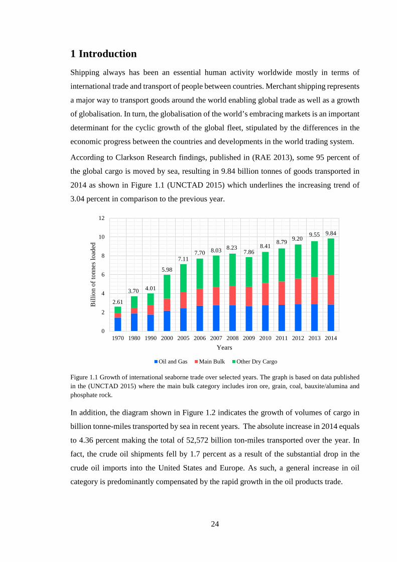
According to Clarkson Research findings, published in (RAE 2013), some 95 percent of
the global cargo is moved by sea, resulting in 9.84 billion tonnes of goods transported in
2014 as shown in Figure 1.1 (UNCTAD 2015) which underlines the increasing trend of
3.04 percent in comparison to the previous year.
Figure 1.1 Growth of international seaborne trade over selected years. The graph is based on data published in the (UNCTAD 2015) where the main bulk category includes iron ore, grain, coal, bauxite/alumina and phosphate rock.
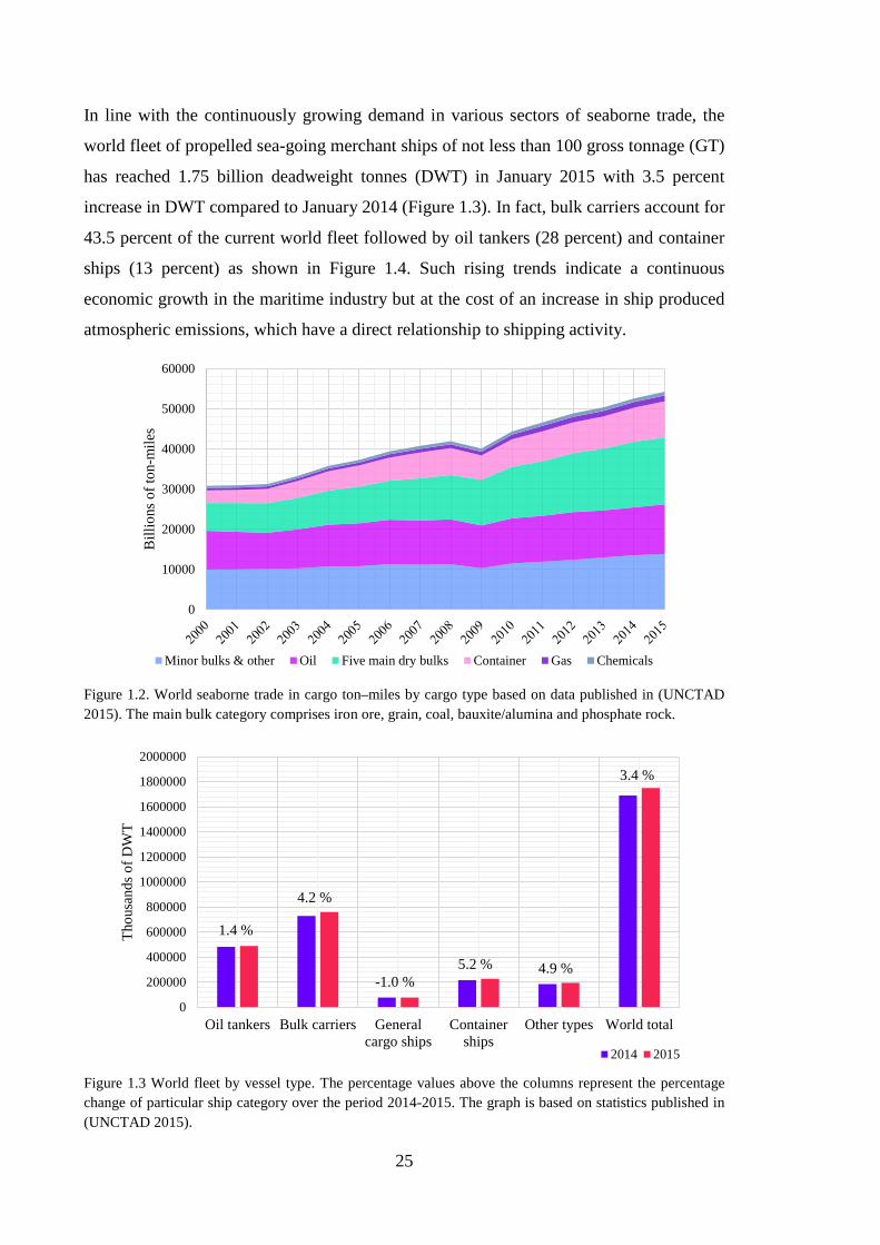
In addition, the diagram shown in Figure 1.2 indicates the growth of volumes of cargo in
billion tonne-miles transported by sea in recent years. The absolute increase in 2014 equals
to 4.36 percent making the total of 52,572 billion ton-miles transported over the year. In
fact, the crude oil shipments fell by 1.7 percent as a result of the substantial drop in the
crude oil imports into the United States and Europe. As such, a general increase in oil
category is predominantly compensated by the rapid growth in the oil products trade.
2.61
3.70 4.01
5.98
7.117.70 8.03 8.23
7.868.41
8.79 9.209.55 9.84
0
2
4
6
8
10
12
1970 1980 1990 2000 2005 2006 2007 2008 2009 2010 2011 2012 2013 2014
Bill
ion
of to
nnes
load
ed
Years
Oil and Gas Main Bulk Other Dry Cargo
25
In line with the continuously growing demand in various sectors of seaborne trade, the
world fleet of propelled sea-going merchant ships of not less than 100 gross tonnage (GT)
has reached 1.75 billion deadweight tonnes (DWT) in January 2015 with 3.5 percent
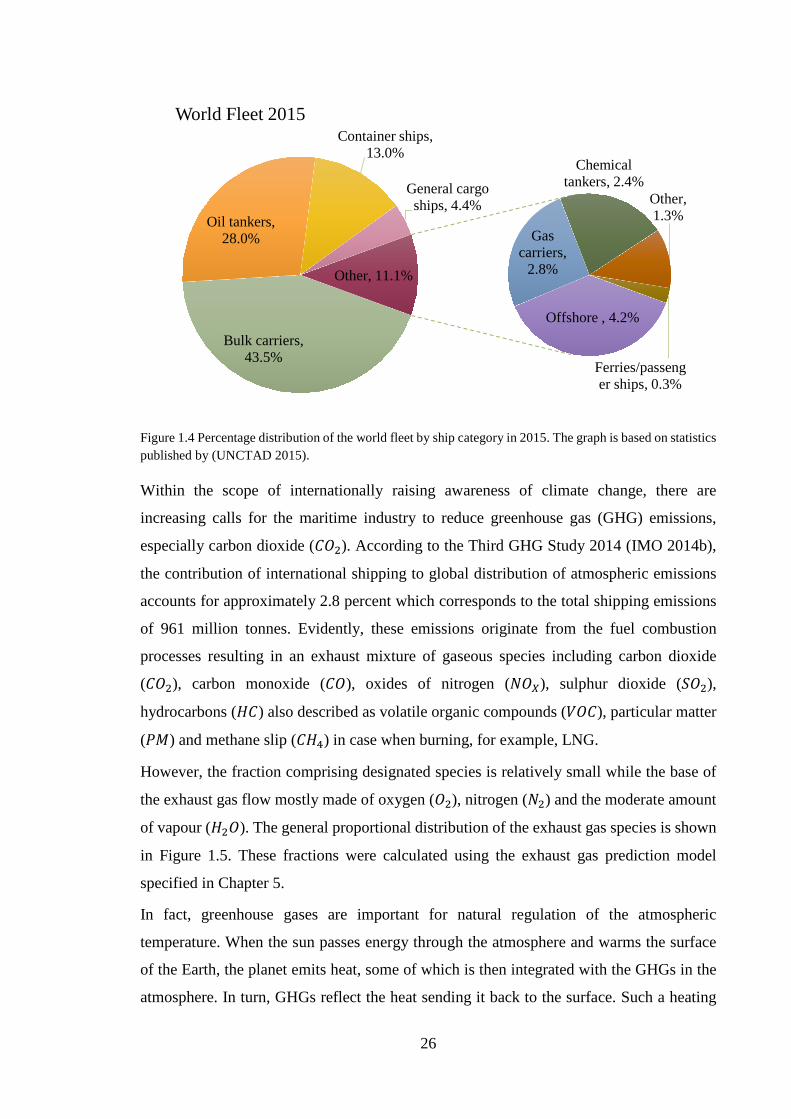
increase in DWT compared to January 2014 (Figure 1.3). In fact, bulk carriers account for
43.5 percent of the current world fleet followed by oil tankers (28 percent) and container
ships (13 percent) as shown in Figure 1.4. Such rising trends indicate a continuous
economic growth in the maritime industry but at the cost of an increase in ship produced
atmospheric emissions, which have a direct relationship to shipping activity.
Figure 1.2. World seaborne trade in cargo ton–miles by cargo type based on data published in (UNCTAD 2015). The main bulk category comprises iron ore, grain, coal, bauxite/alumina and phosphate rock.
Figure 1.3 World fleet by vessel type. The percentage values above the columns represent the percentage change of particular ship category over the period 2014-2015. The graph is based on statistics published in (UNCTAD 2015).
0
10000
20000
30000
40000
50000
60000
Bill
ions
of t
on-m
iles
Minor bulks & other Oil Five main dry bulks Container Gas Chemicals
1.4 %
4.2 %
-1.0 %5.2 % 4.9 %
3.4 %
0
200000
400000
600000
800000
1000000
1200000
1400000
1600000
1800000
2000000
Oil tankers Bulk carriers Generalcargo ships
Containerships
Other types World total
Thou
sand
s of D
WT
2014 2015
26
Figure 1.4 Percentage distribution of the world fleet by ship category in 2015. The graph is based on statistics published by (UNCTAD 2015).
Within the scope of internationally raising awareness of climate change, there are
increasing calls for the maritime industry to reduce greenhouse gas (GHG) emissions,
especially carbon dioxide (𝐶𝐶𝐶𝐶2). According to the Third GHG Study 2014 (IMO 2014b),
the contribution of international shipping to global distribution of atmospheric emissions
accounts for approximately 2.8 percent which corresponds to the total shipping emissions
of 961 million tonnes. Evidently, these emissions originate from the fuel combustion
processes resulting in an exhaust mixture of gaseous species including carbon dioxide
(𝐶𝐶𝐶𝐶2), carbon monoxide (𝐶𝐶𝐶𝐶), oxides of nitrogen (𝑁𝑁𝐶𝐶𝑋𝑋), sulphur dioxide (𝑆𝑆𝐶𝐶2),
hydrocarbons (𝐻𝐻𝐶𝐶) also described as volatile organic compounds (𝑁𝑁𝐶𝐶𝐶𝐶), particular matter
(𝑃𝑃𝑁𝑁) and methane slip (𝐶𝐶𝐻𝐻4) in case when burning, for example, LNG.
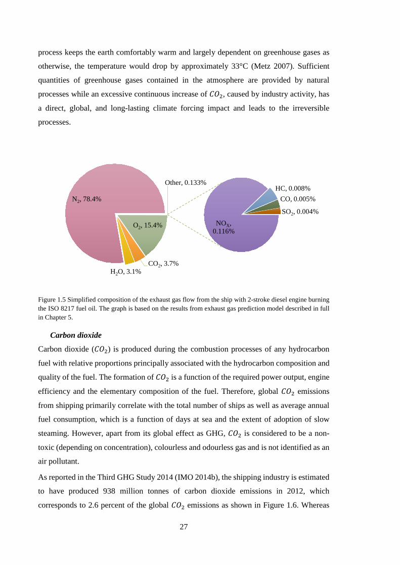
However, the fraction comprising designated species is relatively small while the base of
the exhaust gas flow mostly made of oxygen (𝐶𝐶2), nitrogen (𝑁𝑁2) and the moderate amount
of vapour (𝐻𝐻2𝐶𝐶). The general proportional distribution of the exhaust gas species is shown
in Figure 1.5. These fractions were calculated using the exhaust gas prediction model
specified in Chapter 5.
In fact, greenhouse gases are important for natural regulation of the atmospheric
temperature. When the sun passes energy through the atmosphere and warms the surface
of the Earth, the planet emits heat, some of which is then integrated with the GHGs in the
atmosphere. In turn, GHGs reflect the heat sending it back to the surface. Such a heating
Bulk carriers, 43.5%
Oil tankers, 28.0%
Container ships, 13.0%
General cargo ships, 4.4%
Offshore , 4.2%
Gas carriers,
2.8%
Chemical tankers, 2.4%
Other, 1.3%
Ferries/passenger ships, 0.3%
Other, 11.1%
World Fleet 2015
27
process keeps the earth comfortably warm and largely dependent on greenhouse gases as
otherwise, the temperature would drop by approximately 33°C (Metz 2007). Sufficient
quantities of greenhouse gases contained in the atmosphere are provided by natural
processes while an excessive continuous increase of 𝐶𝐶𝐶𝐶2, caused by industry activity, has
a direct, global, and long-lasting climate forcing impact and leads to the irreversible
processes.
Figure 1.5 Simplified composition of the exhaust gas flow from the ship with 2-stroke diesel engine burning the ISO 8217 fuel oil. The graph is based on the results from exhaust gas prediction model described in full in Chapter 5.
Carbon dioxide
Carbon dioxide (𝐶𝐶𝐶𝐶2) is produced during the combustion processes of any hydrocarbon
fuel with relative proportions principally associated with the hydrocarbon composition and
quality of the fuel. The formation of 𝐶𝐶𝐶𝐶2 is a function of the required power output, engine
efficiency and the elementary composition of the fuel. Therefore, global 𝐶𝐶𝐶𝐶2 emissions
from shipping primarily correlate with the total number of ships as well as average annual
fuel consumption, which is a function of days at sea and the extent of adoption of slow
steaming. However, apart from its global effect as GHG, 𝐶𝐶𝐶𝐶2 is considered to be a non-
toxic (depending on concentration), colourless and odourless gas and is not identified as an
air pollutant.
As reported in the Third GHG Study 2014 (IMO 2014b), the shipping industry is estimated
to have produced 938 million tonnes of carbon dioxide emissions in 2012, which
corresponds to 2.6 percent of the global 𝐶𝐶𝐶𝐶2 emissions as shown in Figure 1.6. Whereas
O2, 15.4%
CO2, 3.7%H2O, 3.1%
N2, 78.4%
NOX, 0.116%
HC, 0.008%CO, 0.005%
SO2, 0.004%
Other, 0.133%
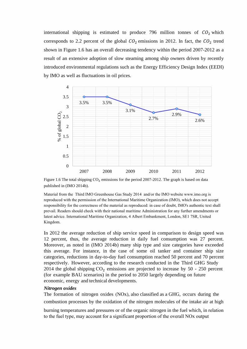
international shipping is estimated to produce 796 million tonnes of 𝐶𝐶𝐶𝐶2 which
corresponds to 2.2 percent of the global 𝐶𝐶𝐶𝐶2 emissions in 2012. In fact, the 𝐶𝐶𝐶𝐶2 trend
shown in Figure 1.6 has an overall decreasing tendency within the period 2007-2012 as a
result of an extensive adoption of slow steaming among ship owners driven by recently
introduced environmental regulations such as the Energy Efficiency Design Index (EEDI)
by IMO as well as fluctuations in oil prices.
Figure 1.6 The total shipping CO2 emissions for the period 2007-2012. The graph is based on data published in (IMO 2014b).
Material from the Third IMO Greenhouse Gas Study 2014 and/or the IMO website www.imo.org is reproduced with the permission of the International Maritime Organization (IMO), which does not accept responsibility for the correctness of the material as reproduced: in case of doubt, IMO's authentic text shall prevail. Readers should check with their national maritime Administration for any further amendments or latest advice. International Maritime Organization, 4 Albert Embankment, London, SE1 7SR, United Kingdom.
In 2012 the average reduction of ship service speed in comparison to design speed was 12 percent, thus, the average reduction in daily fuel consumption was 27 percent. Moreover, as noted in (IMO 2014b) many ship type and size categories have exceeded this average. For instance, in the case of some oil tanker and container ship size categories, reductions in day-to-day fuel consumption reached 50 percent and 70 percent respectively. However, according to the research conducted in the Third GHG Study 2014 the global shipping CO2 emissions are projected to increase by 50 - 250 percent (for example BAU scenarios) in the period to 2050 largely depending on future economic, energy and technical developments. Nitrogen oxides The formation of nitrogen oxides (NOx), also classified as a GHG, occurs during thecombustion processes by the oxidation of the nitrogen molecules of the intake air at high
burning temperatures and pressures or of the organic nitrogen in the fuel which, in relation to the fuel type, may account for a significant proportion of the overall NOx output
relation to the fuel type, may account for a significant proportion of the overall 𝑋𝑋
output
3.5% 3.5%
3.1%
2.7%2.9%
2.6%
0
0.5
1
1.5
2
2.5
3
3.5
4
2007 2008 2009 2010 2011 2012
% o
f glo
bal C
O2
29
especially in case of burning heavy fuel oil. Oxides of nitrogen are often described as 𝑁𝑁𝐶𝐶𝑋𝑋
in order to express the possibility of different combinations of nitrogen and oxygen, which,
in most cases, are nitric oxide (𝑁𝑁𝐶𝐶) or nitrogen dioxide (𝑁𝑁𝐶𝐶2). In fact, when an excess air
is present during the combustion process, 𝑁𝑁𝐶𝐶 is being oxidized into 𝑁𝑁𝐶𝐶2, which has much
more toxicity. Therefore, the formation of 𝑁𝑁𝐶𝐶𝑋𝑋 is a complex process being a non-linear
function of the burning temperature (over 1200°C), pressure, the engine load, air excess
ratio as well as the humidity of the charge air.
Oxides of nitrogen (𝑁𝑁𝐶𝐶𝑋𝑋) along with carbon monoxide (𝐶𝐶𝐶𝐶) and emissions of volatile
organic compounds lead to the formation of tropospheric ozone (𝐶𝐶3) (Torvanger et al.
2007), which has a negative impact on plants and trees, agricultural crop yields and building
materials (Gazley 2007). Moreover, ozone is known to have negative health effects and
promotes development of harmful diseases such as irritation of the respiratory system,
causing coughing and a chest pain, reduced lung function and asthma.
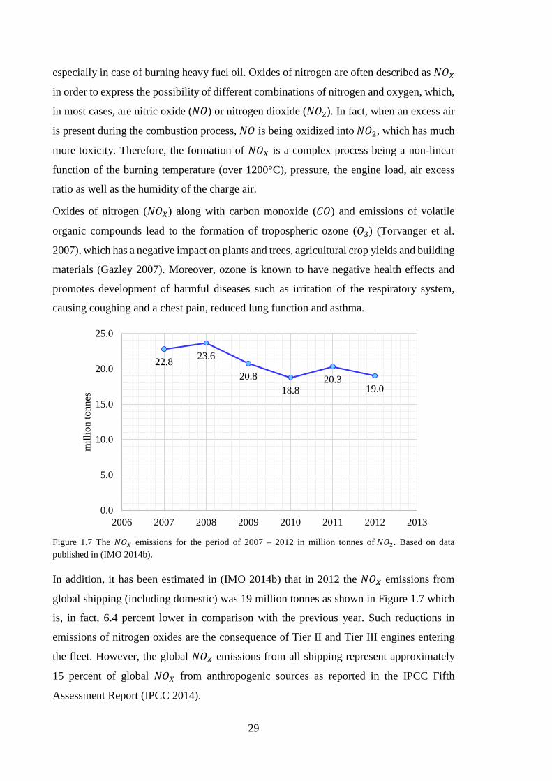
Figure 1.7 The 𝑁𝑁𝐶𝐶𝑋𝑋 emissions for the period of 2007 – 2012 in million tonnes of 𝑁𝑁𝐶𝐶2. Based on data published in (IMO 2014b).
In addition, it has been estimated in (IMO 2014b) that in 2012 the 𝑁𝑁𝐶𝐶𝑋𝑋 emissions from
global shipping (including domestic) was 19 million tonnes as shown in Figure 1.7 which
is, in fact, 6.4 percent lower in comparison with the previous year. Such reductions in
emissions of nitrogen oxides are the consequence of Tier II and Tier III engines entering
the fleet. However, the global 𝑁𝑁𝐶𝐶𝑋𝑋 emissions from all shipping represent approximately
15 percent of global 𝑁𝑁𝐶𝐶𝑋𝑋 from anthropogenic sources as reported in the IPCC Fifth
Assessment Report (IPCC 2014).
22.8 23.6
20.818.8
20.319.0
0.0
5.0
10.0
15.0
20.0
25.0
2006 2007 2008 2009 2010 2011 2012 2013
mill
ion
tonn
es
30
Sulphur oxides
Generally, the marine fuel oils contain a relatively high percentage of sulphur, when
compared to other fuels and, as a result, form sulphur dioxide 𝑆𝑆𝐶𝐶2, which then, in a much
smaller proportion of approximately 3.5 percent, is further oxidized into the sulphur
trioxide 𝑆𝑆𝐶𝐶3. The negative effect of 𝑆𝑆𝐶𝐶𝑋𝑋 emissions is similar to 𝑁𝑁𝐶𝐶𝑋𝑋 comprising human
respiration deceases, harmful effects on vegetation and construction materials. In addition,
the sulphur dioxide particles may also transform into sulphate (𝑆𝑆𝐶𝐶4) (Torvanger et al.
2007), which is the dominant component of aerosol in the atmosphere caused by marine
emissions (Corbett & Winebrake 2008). The particles of 𝑆𝑆𝐶𝐶4 reflect the solar radiation, and
result in Cloud Condensation Nuclei (CCN).
The CCN is a process whereby the marine exhaust emissions increase the number of
particles in the atmosphere over the ocean. Consequently, it increases the number
of water droplets in a volume of cloud, and hence droplets become smaller and the cloud
reflects more sunlight back into space (Crist 2009) while the cloud seems to be optically
brighter (Corbett et al. 2009). This process is called the first indirect effect of sulphate.
Remarkably, in the atmosphere, the sulphur oxides tend to dissolve relatively fast and have
an average lifetime of just two days.
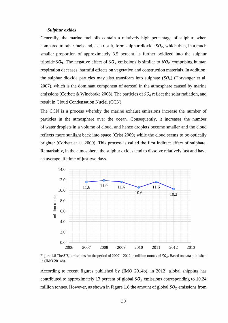
Figure 1.8 The 𝑆𝑆𝐶𝐶𝑋𝑋 emissions for the period of 2007 – 2012 in million tonnes of 𝑆𝑆𝐶𝐶2. Based on data published in (IMO 2014b).
According to recent figures published by (IMO 2014b), in 2012 global shipping has
contributed to approximately 13 percent of global 𝑆𝑆𝐶𝐶𝑋𝑋 emissions corresponding to 10.24
million tonnes. However, as shown in Figure 1.8 the amount of global 𝑆𝑆𝐶𝐶𝑋𝑋 emissions from
11.6 11.9 11.610.6
11.6
10.2
0.0
2.0
4.0
6.0
8.0
10.0
12.0
14.0
2006 2007 2008 2009 2010 2011 2012 2013
mill
ion
tonn
es
31
shipping in 2012 has decreased by 12 percent in comparison to 2011 as a result of new
stricter regulations for reduction of 𝑆𝑆𝐶𝐶𝑋𝑋 which came into force from 1st of January 2012
and will continue to tighten in the coming years. The regulations, as stated in MARPOL
Annex IV (regulation 14), are imposing a strict limitations of sulphur content in fuels being
used for marine applications or engaging to use some additional technologies for reduction
of excess sulphur from the exhaust gas.
Carbon monoxide
Similar to 𝐶𝐶𝐶𝐶2, the carbon monoxide (𝐶𝐶𝐶𝐶) emissions are the result of the combustion
process of hydrocarbon based fossil fuel. The major difference is that 𝐶𝐶𝐶𝐶2 is formed by a
complete oxidation of the carbon molecules in the fuel while 𝐶𝐶𝐶𝐶 comes from the
incomplete combustion due to local areas of air supply deficiency. As such, its formation
in the combustion process is primarily a function of the excess air ratio, the burning
temperature and the homogeneity of the air/fuel mixture in the combustion chamber. In
practice, due to oversupply of excess air for the combustion process, the 𝐶𝐶𝐶𝐶 emissions are
low. However, the concentration of 𝐶𝐶𝐶𝐶 varies with engine load and could be expected to
increase at low loads or in poorly maintained engines.
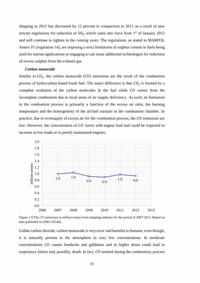
Figure 1.9 The 𝐶𝐶𝐶𝐶 emissions in million tonnes from shipping industry for the period of 2007-2012. Based on data published in (IMO 2014b).
Unlike carbon dioxide, carbon monoxide is very toxic and harmful to humans, even though,
it is naturally present in the atmosphere in very low concentrations. In moderate
concentrations 𝐶𝐶𝐶𝐶 causes headache and giddiness and in higher doses could lead to
respiratory failure and, possibly, death. In fact, 𝐶𝐶𝐶𝐶 emitted during the combustion, process
1.0 1.00.9 0.9
1.0 0.9
0.0
0.2
0.4
0.6
0.8
1.0
1.2
1.4
1.6
1.8
2.0
2006 2007 2008 2009 2010 2011 2012 2013
mill
ion
tonn
es
32
does not transform into 𝐶𝐶𝐶𝐶2 but may react with radicals in the air and, in some cases,
contribute to the formation of ground level ozone. However, its environmental impact is
not fully estimated but suspected to have a marginal effect on climate change. The global
contribution of 𝐶𝐶𝐶𝐶 emissions from the shipping industry has been relatively constant over
recent years and shown on Figure 1.9.
Hydrocarbons
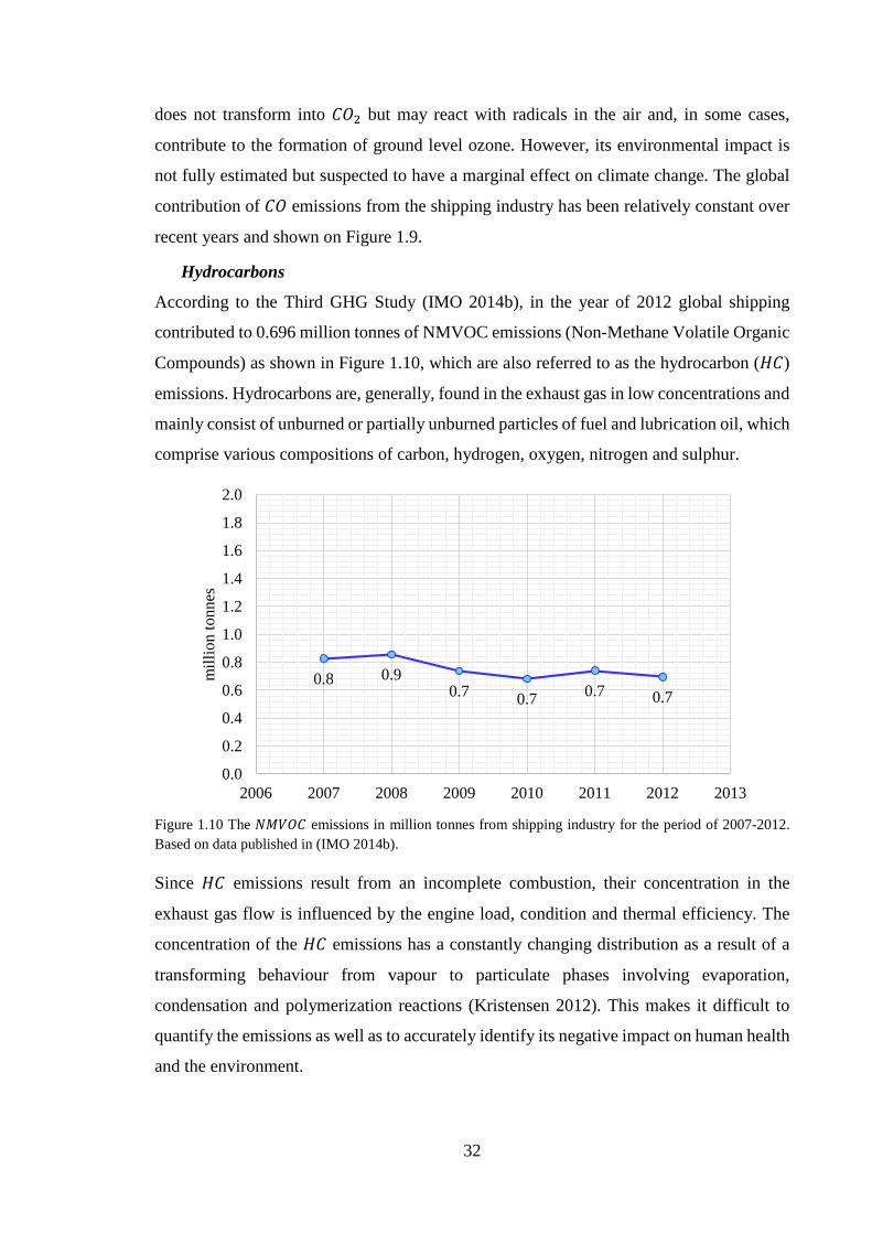
According to the Third GHG Study (IMO 2014b), in the year of 2012 global shipping
contributed to 0.696 million tonnes of NMVOC emissions (Non-Methane Volatile Organic
Compounds) as shown in Figure 1.10, which are also referred to as the hydrocarbon (𝐻𝐻𝐶𝐶)
emissions. Hydrocarbons are, generally, found in the exhaust gas in low concentrations and
mainly consist of unburned or partially unburned particles of fuel and lubrication oil, which
comprise various compositions of carbon, hydrogen, oxygen, nitrogen and sulphur.
Figure 1.10 The 𝑁𝑁𝑁𝑁𝑁𝑁𝐶𝐶𝐶𝐶 emissions in million tonnes from shipping industry for the period of 2007-2012. Based on data published in (IMO 2014b).
Since 𝐻𝐻𝐶𝐶 emissions result from an incomplete combustion, their concentration in the
exhaust gas flow is influenced by the engine load, condition and thermal efficiency. The
concentration of the 𝐻𝐻𝐶𝐶 emissions has a constantly changing distribution as a result of a
transforming behaviour from vapour to particulate phases involving evaporation,
condensation and polymerization reactions (Kristensen 2012). This makes it difficult to
quantify the emissions as well as to accurately identify its negative impact on human health
and the environment.
0.8 0.90.7 0.7 0.7 0.7
0.0
0.2
0.4
0.6
0.8
1.0
1.2
1.4
1.6
1.8
2.0
2006 2007 2008 2009 2010 2011 2012 2013
mill
ion
tonn
es
33
Generally, hydrocarbon emissions are highly toxic and found to have mutagenesis and
carcinogenesis properties. In terms of environmental effects, the volatile organic
compounds are engaged in photochemical reactions contributing to the formation of
tropospheric ozone and global climate change.
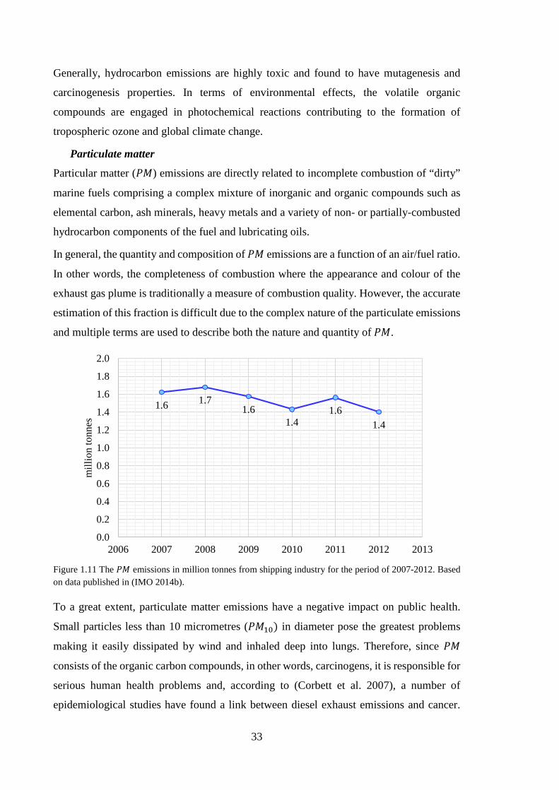
Particulate matter
Particular matter (𝑃𝑃𝑁𝑁) emissions are directly related to incomplete combustion of “dirty”
marine fuels comprising a complex mixture of inorganic and organic compounds such as
elemental carbon, ash minerals, heavy metals and a variety of non- or partially-combusted
hydrocarbon components of the fuel and lubricating oils.
In general, the quantity and composition of 𝑃𝑃𝑁𝑁 emissions are a function of an air/fuel ratio.
In other words, the completeness of combustion where the appearance and colour of the
exhaust gas plume is traditionally a measure of combustion quality. However, the accurate
estimation of this fraction is difficult due to the complex nature of the particulate emissions
and multiple terms are used to describe both the nature and quantity of 𝑃𝑃𝑁𝑁.
Figure 1.11 The 𝑃𝑃𝑁𝑁 emissions in million tonnes from shipping industry for the period of 2007-2012. Based on data published in (IMO 2014b).
To a great extent, particulate matter emissions have a negative impact on public health.
Small particles less than 10 micrometres (𝑃𝑃𝑁𝑁10) in diameter pose the greatest problems
making it easily dissipated by wind and inhaled deep into lungs. Therefore, since 𝑃𝑃𝑁𝑁
consists of the organic carbon compounds, in other words, carcinogens, it is responsible for
serious human health problems and, according to (Corbett et al. 2007), a number of
epidemiological studies have found a link between diesel exhaust emissions and cancer.
1.6 1.71.6
1.41.6
1.4
0.0
0.2
0.4
0.6
0.8
1.0
1.2
1.4
1.6
1.8
2.0
2006 2007 2008 2009 2010 2011 2012 2013
mill
ion
tonn
es

34
For instance, (Lauer et al. 2007) in the “Mortality from Ship Emissions: A Global
Assessment” concluded that particulates from shipping industry could cause lung cancer
and cardiopulmonary diseases that lead to premature death of approximately 60,000 people
annually. In fact, as estimated in the Third GHG Study 2014 (IMO 2014b), 𝑃𝑃𝑁𝑁 amounts
from the global shipping in 2012 equal to 1.4 million tonnes (Figure 1.11).
As such, the exhaust emissions from the shipping industry, along with the atmospheric
emissions contributed by other industries, affect radiative forcing of the climate (RF),
which is the conventional climate metric, expressed in watts per square metre, and used in
climate science. RF represents a change in the energy budget of the atmosphere relative to
1750, by the definition of the Intergovernmental Panel on Climate Change (IPCC). In other
words, radiative forcing identifies the change in the balance between radiation coming into
the atmosphere and radiation going out (MEPC 53th Session & Agenda Item 4 2005).
Radiative forcing is usually expressed as a global mean, and positive numbers denote
warming while negative numbers denote cooling. The effects of marine emissions on
radiative forcing are as follows:
- The CO2 emissions have a warming effect and positive radiative forcing (RF);
- The emissions of 𝑁𝑁𝐶𝐶𝑋𝑋 result in the formation of tropospheric ozone 𝐶𝐶3 with the
positive effect to RF (Torvanger et al. 2007).
- The oxides of sulphur (𝑆𝑆𝐶𝐶𝑋𝑋) have a negative direct RF.
- The 𝑃𝑃𝑁𝑁 particles and 𝐻𝐻𝐶𝐶 emissions have a positive direct and indirect effect (for
example snow) RF (Corbett et al. 2009).
The overall impact of exhaust emissions on the atmosphere, as schematically represented
in Figure 1.12, is rather complex but clearly leads to the increase of its impurity content
while disturbing its natural balance. Through the atmospheric reactions, the emitted
particles may be involved in various microphysical processes or be removed by land or
water surfaces through dry or wet deposition while further affecting its radiative balance.
Such imbalance in radiative forcing may impact a climate in different ways including the
global and local mean surface temperature, sea level, changes in precipitation, snow and
ice cover and more. In turn, these physical impacts may have social implications through
their effects on agriculture, forestry, energy production, human health, etc. Finally, all these
effects have a social cost, which can be difficult to estimate.
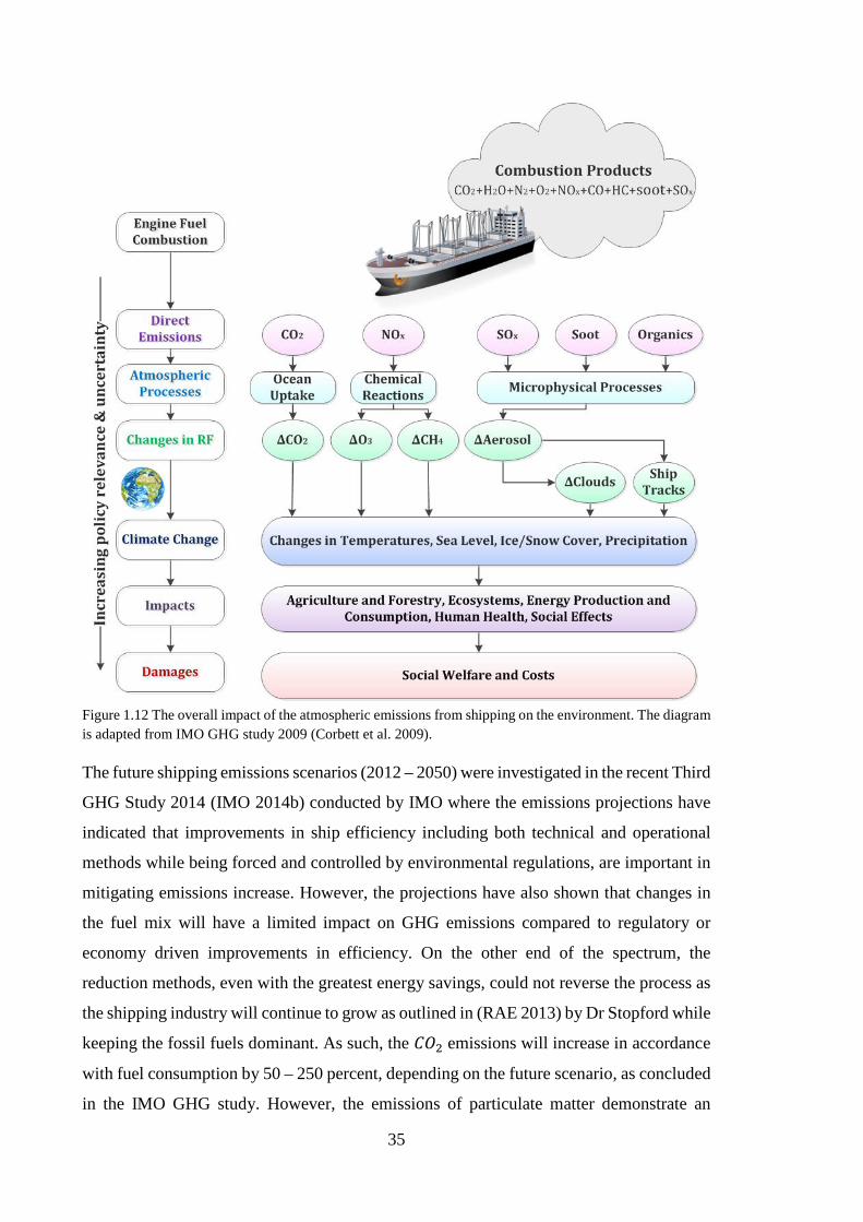
35
Figure 1.12 The overall impact of the atmospheric emissions from shipping on the environment. The diagram is adapted from IMO GHG study 2009 (Corbett et al. 2009).
The future shipping emissions scenarios (2012 – 2050) were investigated in the recent Third
GHG Study 2014 (IMO 2014b) conducted by IMO where the emissions projections have
indicated that improvements in ship efficiency including both technical and operational
methods while being forced and controlled by environmental regulations, are important in
mitigating emissions increase. However, the projections have also shown that changes in
the fuel mix will have a limited impact on GHG emissions compared to regulatory or
economy driven improvements in efficiency. On the other end of the spectrum, the
reduction methods, even with the greatest energy savings, could not reverse the process as
the shipping industry will continue to grow as outlined in (RAE 2013) by Dr Stopford while
keeping the fossil fuels dominant. As such, the 𝐶𝐶𝐶𝐶2 emissions will increase in accordance
with fuel consumption by 50 – 250 percent, depending on the future scenario, as concluded
in the IMO GHG study. However, the emissions of particulate matter demonstrate an
36
absolute decrease up to 2020 as well as oxides of sulphur continue to decline through to
2050, primarily because of MARPOL Annex VI requirements on the sulphur content in
fuels.
In the context of the environmental protection activities, the situation with the development
of a global climate policy framework to control the ship produced emissions is very
complicated mainly due to its international nature. In particular, one certain aspect makes
the shipping industry a very complex issue since every ship is registered to a specific Flag
State that could be different from the owner’s country and nationality. One of the reasons
for this phenomenon is that the ship owners are likely to register their vessels in
the most favourable tax jurisdiction rather than their country of origin or their operational
headquarter. For instance, it wouldn’t be unusual for a ship to be built in China, owned by
a company based in the United Kingdom managed by a Greek ship owner and, at the same
time, registered under the Panamanian Flag in order to move goods from India to Italy.
According to statistics compiled by the UNCTAD secretariat on the basis of data supplied
by Clarkson Research (UNCTAD 2015) as of 1st January 2015 the top 10 ship registries
control about 51.3 percent of the total world fleet by the number of ships and approximately
76.7 percent of the world’s fleet total DWT (Figure 1.13). Whilst Panama dominates the
world fleet by the country of registration, the list of world’s top ship owning countries is
very different as shown in Figure 1.14. These top 10 countries by ownership together
control 67 percent of the total DWT with the United Kingdom taking up the 8th position. In
fact, according to (UNCTAD 2015), for 11.8 percent of the world fleet in DWT, the
owner’s nationality differs from the country of ownership. All these circumstances could
be explained by having a deeper look into the framework of the international maritime law
and regulations.
In order to understand the general principles of maritime regulations, it is important to note
that maritime activities such as international shipping are regulated not only by the
international law of the sea but also by the law of a particular country (State). The United
Nations Convention on the Law of the Sea (UNCLOS) is the cornerstone of international
maritime law. UNCLOS endorses the right of any sovereign State to have a ship register
and thus become a Flag State, and it provides ships with the right to innocent passage
through territorial waters and economic zones (Corbett et al. 2009). International law
regulates maritime activities in a particular Flag State but does not apply directly to
individual vessels.
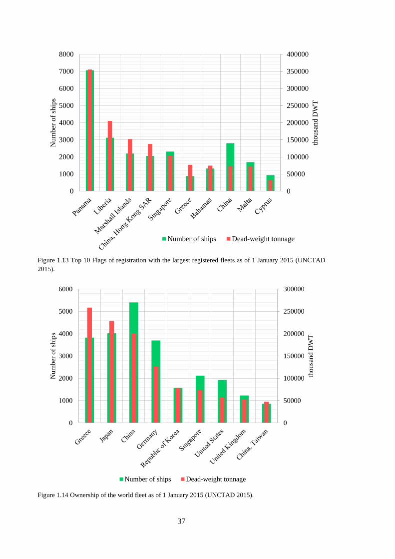
37
Figure 1.13 Top 10 Flags of registration with the largest registered fleets as of 1 January 2015 (UNCTAD 2015).
Figure 1.14 Ownership of the world fleet as of 1 January 2015 (UNCTAD 2015).
0
50000
100000
150000
200000
250000
300000
350000
400000
0
1000
2000
3000
4000
5000
6000
7000
8000
thou
sand
DW
T
Num
ber o
f shi
ps
Number of ships Dead-weight tonnage
0
50000
100000
150000
200000
250000
300000
0
1000
2000
3000
4000
5000
6000
thou
sand
DW
T
Num
ber o
f shi
ps
Number of ships Dead-weight tonnage
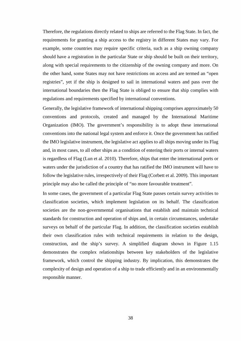
38
Therefore, the regulations directly related to ships are referred to the Flag State. In fact, the
requirements for granting a ship access to the registry in different States may vary. For
example, some countries may require specific criteria, such as a ship owning company
should have a registration in the particular State or ship should be built on their territory,
along with special requirements to the citizenship of the owning company and more. On
the other hand, some States may not have restrictions on access and are termed an “open
registries”, yet if the ship is designed to sail in international waters and pass over the
international boundaries then the Flag State is obliged to ensure that ship complies with
regulations and requirements specified by international conventions.
Generally, the legislative framework of international shipping comprises approximately 50
conventions and protocols, created and managed by the International Maritime
Organization (IMO). The government’s responsibility is to adopt these international
conventions into the national legal system and enforce it. Once the government has ratified
the IMO legislative instrument, the legislative act applies to all ships moving under its Flag
and, in most cases, to all other ships as a condition of entering their ports or internal waters
is regardless of Flag (Lun et al. 2010). Therefore, ships that enter the international ports or
waters under the jurisdiction of a country that has ratified the IMO instrument will have to
follow the legislative rules, irrespectively of their Flag (Corbett et al. 2009). This important
principle may also be called the principle of “no more favourable treatment”.
In some cases, the government of a particular Flag State passes certain survey activities to
classification societies, which implement legislation on its behalf. The classification
societies are the non-governmental organisations that establish and maintain technical
standards for construction and operation of ships and, in certain circumstances, undertake
surveys on behalf of the particular Flag. In addition, the classification societies establish
their own classification rules with technical requirements in relation to the design,
construction, and the ship’s survey. A simplified diagram shown in Figure 1.15
demonstrates the complex relationships between key stakeholders of the legislative
framework, which control the shipping industry. By implication, this demonstrates the
complexity of design and operation of a ship to trade efficiently and in an environmentally
responsible manner.
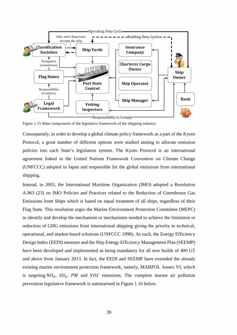
39
Only until shipowner accepts the ship
Figure 1.15 Main components of the legislative framework of the shipping industry.
Consequently, in order to develop a global climate policy framework as a part of the Kyoto
Protocol, a great number of different options were studied aiming to allocate emission
policies into each State’s legislation system. The Kyoto Protocol is an international
agreement linked to the United Nations Framework Convention on Climate Change
(UNFCCC) adopted in Japan and responsible for the global emissions from international
shipping.
Instead, in 2003, the International Maritime Organization (IMO) adopted a Resolution
A.963 (23) on IMO Policies and Practices related to the Reduction of Greenhouse Gas
Emissions from Ships which is based on equal treatment of all ships, regardless of their
Flag State. This resolution urges the Marine Environment Protection Committee (MEPC)
to identify and develop the mechanism or mechanisms needed to achieve the limitation or
reduction of GHG emissions from international shipping giving the priority to technical,
operational, and market-based solutions (UNFCCC 1998). As such, the Energy Efficiency
Design Index (EEDI) measure and the Ship Energy Efficiency Management Plan (SEEMP)
have been developed and implemented as being mandatory for all new builds of 400 GT
and above from January 2013. In fact, the EEDI and SEEMP have extended the already
existing marine environment protection framework, namely, MARPOL Annex VI, which
is targeting 𝑁𝑁𝐶𝐶𝑋𝑋, 𝑆𝑆𝐶𝐶𝑋𝑋, 𝑃𝑃𝑁𝑁 and 𝑁𝑁𝐶𝐶𝐶𝐶 emissions. The complete marine air pollution
prevention legislative framework is summarised in Figure 1.16 below.
40
IMO Marine Environment Protection Committee (MEPC)
GHG Emissions(CO2 and other)
SOx NOx
Non ECAECA
2012 Sulphur
content < 3.5%
EEDI SEEMP
2020 Sulphur
content < 0.5%
2012 Sulphur
content < 1%
2015 Sulphur
content < 0.1%
SOx NOx
1990 - 2000TIER I engines
2011TIER II engines
2016TIER III engines
Phase 0 – 2013implementation
Phase 1 – 201510% reduction
Phase 2 – 202020% reduction
Phase 3 – 202530% reduction
Planning
Implementing
Monitoring
Self-evaluating
Improving
EEOI
• Baltic Sea (SOx)• North Sea (SOx)• North American ECA
(SOx, NOx, PM)• US Caribbean Sea ECA
(SOx, NOx, PM)
Energy Efficiency Data
Collection System
MARPOL ANNEX VIAir Pollution (NOx SOx VOC PM)
Figure 1.16 IMO air pollution prevention legislative framework.
Both mechanisms, which can be associated with the energy efficiency and emissions
standards, are the first ever mandatory GHG regulations for the shipping industry. While
the EEDI imposes an energy efficiency criterion for new ships, which, when implemented,
would have to be verified against the defined standard by an independent organisation in
order to obtain certification, the SEEMP enables ship owners to measure the fuel efficiency
of existing ships and to monitor the effects of any changes in operation.
Energy Efficiency Design Index
In simplest terms, the EEDI can be described as the ratio between 𝐶𝐶𝐶𝐶2 production potential
of the ship and its benefit to society. Whereas, the 𝐶𝐶𝐶𝐶2 production potential comprises the
𝐶𝐶𝐶𝐶2 associated with the ship’s main propulsion, auxiliary and hotel power consumption
including the expected benefits from the energy efficiency technologies that generate
additional electrical power such as waste heat recovery system (WHRS) minus the
innovative energy efficiency technologies incorporated in the design for example wind
assistance or a hull air lubricating system added to enhance the propulsive efficiency of the
ship. The benefit to society is a function of the ship’s speed and its cargo carrying capacity.
The EEDI also includes a number of correction factors that have been introduced for
specific ship types or particular design features. However, the formula is presently not
applicable to ships with diesel-electric propulsion, turbine propulsion or a hybrid
propulsion system, except for cruise passenger ships and liquefied natural gas (LNG)
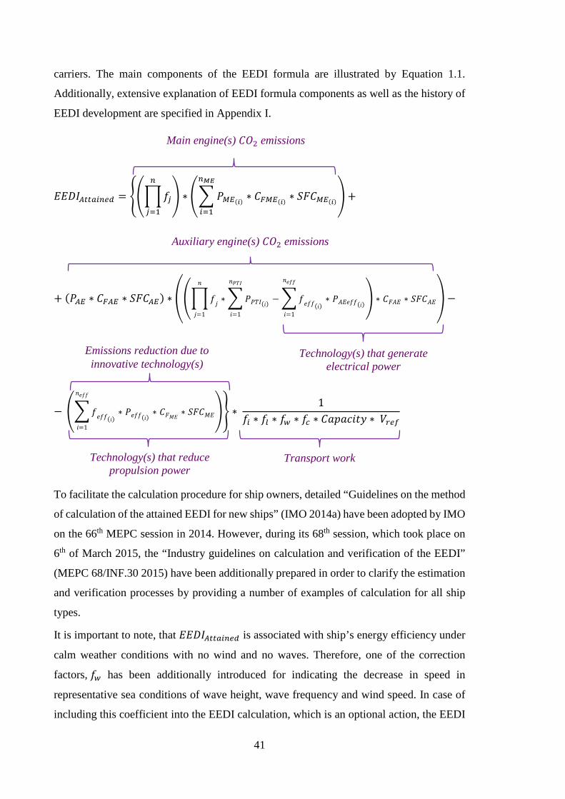
41
carriers. The main components of the EEDI formula are illustrated by Equation 1.1.
Additionally, extensive explanation of EEDI formula components as well as the history of
EEDI development are specified in Appendix I.
𝐸𝐸𝐸𝐸𝐷𝐷𝐸𝐸𝐴𝐴𝐴𝐴𝐴𝐴𝑔𝑔𝐴𝐴𝐴𝐴𝐴𝐴𝐴𝐴 = 𝑓𝑓𝑗𝑗
𝐴𝐴
𝑗𝑗=1
∗ 𝑃𝑃𝑀𝑀𝐸𝐸(𝑖𝑖) ∗ 𝐶𝐶𝐹𝐹𝑀𝑀𝐸𝐸(𝑖𝑖) ∗ 𝑆𝑆𝑆𝑆𝐶𝐶𝑀𝑀𝐸𝐸(𝑖𝑖)
𝐴𝐴𝑀𝑀𝑀𝑀
𝐴𝐴=1
+
+ (𝑃𝑃𝐴𝐴𝐸𝐸 ∗ 𝐶𝐶𝐹𝐹𝐴𝐴𝐸𝐸 ∗ 𝑆𝑆𝑆𝑆𝐶𝐶𝐴𝐴𝐸𝐸) ∗ 𝑓𝑓𝑗𝑗
𝑛𝑛
𝑗𝑗=1
∗𝑃𝑃𝑃𝑃𝑃𝑃𝐸𝐸(𝑖𝑖) −𝑓𝑓𝑒𝑒𝑓𝑓𝑓𝑓(𝑖𝑖)∗ 𝑃𝑃𝐵𝐵𝐸𝐸𝑒𝑒𝑓𝑓𝑓𝑓(𝑖𝑖)
𝑛𝑛𝑒𝑒𝑓𝑓𝑓𝑓
𝑖𝑖=1
𝑛𝑛𝑃𝑃𝑃𝑃𝐸𝐸
𝑖𝑖=1
∗ 𝐶𝐶𝑆𝑆𝐵𝐵𝐸𝐸 ∗ 𝑆𝑆𝑆𝑆𝐶𝐶𝐵𝐵𝐸𝐸 −
− 𝑓𝑓𝑒𝑒𝑓𝑓𝑓𝑓(𝑖𝑖)∗ 𝑃𝑃𝑒𝑒𝑓𝑓𝑓𝑓(𝑖𝑖)
∗ 𝐶𝐶𝑆𝑆𝑁𝑁𝐸𝐸 ∗ 𝑆𝑆𝑆𝑆𝐶𝐶𝑁𝑁𝐸𝐸
𝑛𝑛𝑒𝑒𝑓𝑓𝑓𝑓
𝑖𝑖=1
∗ 1
𝑓𝑓𝐴𝐴 ∗ 𝑓𝑓𝑙𝑙 ∗ 𝑓𝑓𝑤𝑤 ∗ 𝑓𝑓𝑐𝑐 ∗ 𝐶𝐶𝐻𝐻𝐶𝐶𝐻𝐻𝐶𝐶𝑖𝑖𝐶𝐶𝐶𝐶 ∗ 𝑁𝑁𝑟𝑟𝐴𝐴𝑟𝑟
To facilitate the calculation procedure for ship owners, detailed “Guidelines on the method
of calculation of the attained EEDI for new ships” (IMO 2014a) have been adopted by IMO
on the 66th MEPC session in 2014. However, during its 68th session, which took place on
6th of March 2015, the “Industry guidelines on calculation and verification of the EEDI”
(MEPC 68/INF.30 2015) have been additionally prepared in order to clarify the estimation
and verification processes by providing a number of examples of calculation for all ship
types.
It is important to note, that 𝐸𝐸𝐸𝐸𝐷𝐷𝐸𝐸𝐴𝐴𝐴𝐴𝐴𝐴𝑔𝑔𝐴𝐴𝐴𝐴𝐴𝐴𝐴𝐴 is associated with ship’s energy efficiency under
calm weather conditions with no wind and no waves. Therefore, one of the correction
factors, 𝑓𝑓𝑤𝑤 has been additionally introduced for indicating the decrease in speed in
representative sea conditions of wave height, wave frequency and wind speed. In case of
including this coefficient into the EEDI calculation, which is an optional action, the EEDI
Main engine(s) 𝐶𝐶𝐶𝐶2 emissions
Auxiliary engine(s) 𝐶𝐶𝐶𝐶2 emissions
Emissions reduction due to innovative technology(s)
Technology(s) that reduce propulsion power
Technology(s) that generate electrical power
Transport work

42
index should be specified as 𝐸𝐸𝐸𝐸𝐷𝐷𝐸𝐸𝑊𝑊𝐴𝐴𝑔𝑔𝐴𝐴ℎ𝐴𝐴𝑟𝑟. The detailed guidance on estimating of the 𝑓𝑓𝑤𝑤
coefficient is described in (MEPC.1/Circ.796 2012).
To define the energy efficiency criteria, some parametric studies have been undertaken for
a number of ship types built between 2000 and 2010. As a result, the EEDI reference lines
have been introduced for a range of ship types of various sizes including bulk carrier, gas
carrier, tanker, container ship, general cargo ship, refrigerated cargo carrier, combination
carrier, ro-ro cargo ship, ro-ro cargo ship (vehicle), ro-ro passenger ships and LNG carrier
excluding passenger ships other than cruise passenger ship having non-conventional
propulsion. The reference line methodology is also explained in Appendix I.
The 𝐶𝐶𝐶𝐶2 reduction is expected to be achieved within a phased process such as a reduction
level (grams of 𝐶𝐶𝐶𝐶2 per tonne mile) for the first phase (2015-2019) is set to 10 percent and
will be tightened every five years as outlined in Figure 1.16. Therefore, in order to obtain
an International Energy Efficiency Certificate (IEEC), the 𝐸𝐸𝐸𝐸𝐷𝐷𝐸𝐸𝐴𝐴𝐴𝐴𝐴𝐴𝑔𝑔𝐴𝐴𝐴𝐴𝐴𝐴𝐴𝐴 must be less than
or equal to the 𝐸𝐸𝐸𝐸𝐷𝐷𝐸𝐸𝑅𝑅𝐴𝐴𝑅𝑅𝑅𝑅𝐴𝐴𝑟𝑟𝐴𝐴𝐴𝐴 in accordance to the current reference phase.
Ship Energy Efficiency Management Plan
In turn, the Ship Energy Efficiency Management Plan (SEEMP) is an operational measure
that establishes a mechanism to improve the energy efficiency of a ship in a cost-effective
manner by providing an approach for shipping companies to manage ship and fleet
efficiency performance over time using, for example, the Energy Efficiency Operational
Indicator (EEOI) (MEPC.1/Circ.684 2009) as a monitoring tool.
Generally, the SEEMP approach aims to enhance ship's energy efficiency through the
following steps: planning, implementation, monitoring, and self-evaluation and
improvement. Whereas the EEOI helps to analyse the effect of any changes in operation,
such as an improved voyage planning, by means of the continuous ship performance
monitoring onboard. The SEEMP also invites the ship owner to consider new energy
efficient technologies, for instance, the introduction of a waste heat recovery systems or a
new propeller, for achieving a better performance.
In addition, according to the 68th MEPC session, it has been agreed to develop a global ship
data collection system for fuel consumption of ships of 5000 GT and above in order to
analyse its energy efficiency. The system is planned to include the ship identification
number, technical characteristics, and total annual fuel consumption by the fuel type as
well as transport work. The methodology for collecting the data would be added to the

43
SEEMP (MEPC.213(63) 2012). The annually collected data would be reported by the ship
owner to the Flag State which would submit the data to IMO for inclusion in a database.
Air pollution reduction
The main purpose of the MARPOL Annex VI and the associated 𝑁𝑁𝐶𝐶𝑋𝑋 Technical Code 2008
(MEPC 12th Session & Agenda Item 6 2007), which entered into force on 1 July 2010, is
to identify the emissions standards and to limit air pollution to its maximum particularly in
Emissions Control Areas (ECAs) addressing both new builds and existing ships. As shown
in Figure 1.16, there are four currently active ECAs: Baltic Sea for 𝑆𝑆𝐶𝐶𝑋𝑋, North Sea for 𝑆𝑆𝐶𝐶𝑋𝑋,
North American ECA for 𝑆𝑆𝐶𝐶𝑋𝑋 , 𝑁𝑁𝐶𝐶𝑋𝑋 and 𝑃𝑃𝑁𝑁 and US Caribbean Sea for 𝑆𝑆𝐶𝐶𝑋𝑋, 𝑁𝑁𝐶𝐶𝑋𝑋
and 𝑃𝑃𝑁𝑁. However, some additional ECAs in Singapore, Japan and the Mediterranean
region have been appointed to enter into force in the coming years. As such, for ECAs the
maximum sulphur content in fuels must be under or equal 0.1 percent which came into
force from 1st January 2015. For the areas outside the ECA, the maximum sulphur content
is 3.5 percent and will be further reduced to 0.5 percent by 1st January 2020.
With regard to the reduction of 𝑁𝑁𝐶𝐶𝑋𝑋 emissions from marine diesel engines, there are a Tier
II emission limit for engines installed on a ship constructed on or after 1 January 2011 and
a more straightened Tier III emission limit for the engines installed on a ship constructed
on or after 1 January 2016 and operating in ECAs (North American Emission Control Area
and the U.S. Caribbean Sea Emission Control Area). Marine diesel engines installed on a
ship constructed on or after 1 January 1990 but prior to 1 January 2000 are required to
comply with Tier I emission limits.
Clearly, the reductions in exhaust emissions can be achieved through the incorporation of
innovative energy efficient technologies and low-carbon or alternative fuels as well as the
use of renewable power sources in addition to a well-planned operational profile while
taking into account the fluctuations in freight rates and daily fuel costs. However, in such
a hostile environment, there is always a portion of the risk associated with innovative
technologies. As such, in order to achieve full potential efficiency and minimise the rising
uncertainty, a ship must be considered as an integrated engineering system within its
intended operational profile.

44
Research objectives
The primary objective of this PhD research is to develop an advanced understanding of the
necessary and realistic performance expectations from a full form medium size ship system
by means of numerical computer modelling. This includes the minimisation of the harmful
environmental signature by increasing its efficiency in compliance with the EEDI
requirements while in search of how the EEDI methodology might be enhanced. The
investigation has focused on a medium sized products tanker acting as a midpoint of the
spectrum of ship sizes within the range of 20,000 – 60,000 DWT of this type.
In order to solve such an extensive problem, in the first place, it was important to analyse
the energy efficient technology market in a structured manner and then, to identify the most
favourable fuel consumption reduction methods that can be associated with the examined
ship type. Next, an integrated computer simulation model, involving linked engine,
propeller and hull analysis programs, has been developed and calibrated with model tests
and sea trial data. The ship system has been analysed under diverse conditions including
various propulsion systems, innovative machinery arrangements, efficiency-enhancing
hydrodynamic appendages as well as changing weather and load conditions.
The evaluation of potential benefits associated with the deployment of innovative
technology(s), operation profile(s) or their combination has been made by comparing the
designated Energy Efficiency Indicators (EDI), namely, the propulsive efficiency, fuel oil
consumption, exhaust emissions footprint and EEDI, respectively associated with the
technical, fuel savings, environmental and legal perspectives.
In addition, such a comprehensive analysis has also helped to detect a number of
uncertainties in the current EEDI formulation while pointing out ways in which it can be
improved.
45
2 Ship as a System Approach: Methods and Technologies to
Enhance Ship Energy Efficiency
The historical development of merchant shipping has been to a large extent driven by a
constantly increasing demand for greater propulsion efficiency or higher operating speed.
However, due to unstable oil prices as well as rising environmental pressure, the increase
in ship’s speed is no longer the highest priority. This has stimulated a deeper interest in
alternative fuels and propulsion options such as a possibility to burn LNG in reciprocating
engines, incorporating renewable energy technologies, hybrid propulsion and innovative
energy saving appendages with an increasing concern in fuel cells and nuclear power.
A historical analysis of ship design efficiency has been conducted in several studies. The
IMO GHG Study 2009 (Corbett et al. 2009) gives brief analysis of average design
efficiency over time measured in 𝑔𝑔𝐶𝐶𝐶𝐶2 𝐶𝐶𝑡𝑡𝑛𝑛 − 𝑛𝑛𝑛𝑛⁄ , which indicate significant
improvements in ship efficiency over the past century. However, according to historical
curves in (Corbett et al. 2009) the efficiency of cargo ships, container ships in particular,
has slightly declined in the 1990s. Another research, conducted by Mortensen (Mortensen
2009) verifies the overall energy efficiency trend in (Corbett et al. 2009) specifying that
the design efficiency of VLCC tankers improved between 1995 and 2000, but decreased in
the next period, while the efficiency of handy size bulkers does not show any notable trend.
A complete study on ship efficiency historical trends elaborated by (Faber 2015) indicates
that depending on the ship size and type, ship efficiency improved by 22 – 28 percent in
the 1980s, which has been a result of increasing oil prices and relatively low freight rates.
In some cases, the efficiency improvements were stimulated by reductions in design speed
and main engine power or due to increased ship sizes. On the other hand, the overall
efficiency decrease in the 1990s seems to be the result of ship designs where capital costs
and capacity had a greater priority than fuel efficiency, making it comparable to the current
situation of lower oil prices.
Therefore, (Faber 2015) concludes that in order to improve ship efficiency by 5 – 15 percent
it might be beneficial to look back at the 1990s designs. In fact, the design efficiency of
new builds after 2009 have already been supporting this trend, meaning that lower design
speeds could improve efficiency where appropriate. Additionally, technological progress
such as the development of computational fluid dynamics (CFD), although having some
limitations (for example turbulence modelling for thick boundary layers), has significantly

46
contributed to the understanding of hull, propulsion and engine efficiency, indicating the
potential of much greater efficiency improvements to come.
Economical triggers
The overall changes in design efficiency strongly depend upon the global economic
circumstances. One of the most important triggers for the ship owner to invest in the more
energy efficient designs is an increase in oil prices, helping to reduce the total ownership
costs. In fact, as the innovative hull designs are generally more expensive, the amortisation
of the additional investments is shorter when fuel prices are high. Another important factor
is high freight rates that promote yards to build more ships with standard designs at a
potentially low risk with an increased profit margin. In turn, when freight rates are low,
shipyards have to compete for clients offering them more efficient designs.
One of the most significant aspects that slow down demand for more efficient ships among
the ship owners is that in many cases they do not receive a financial reward provided with
the efficiency benefits. The truth is that fuel savings achieved by the energy efficient design
or technologies often belong to the charterer who is actually paying for the fuel. However,
in some cases, the ship owner has to have a competitive ship in order to compete for better
contracts.
The other critical factors that influence ship owners to prefer less efficient ships include
dimensional restrictions in some ports and canals or gaps in the infrastructure, limiting the
maximum cargo capacity. Such limitations have especially negative implications on ship
efficiency under high freight rates and low oil prices. Regardless, a desire for innovations
is strongly influenced by the global environmental policies described in the Introduction.
Ship as a system approach
In order to effectively comply with tightening environmental regulations, it is important for
the ship owner to have a clear picture of what realistically could be achieved by
implementing the innovative technologies and strategies as well as to evaluate possible
risks and benefits while keeping costs to a minimum. Moreover, sometimes it is difficult
for the shipowner to establish what particular design package is the most beneficial as a
wide range of variables should be considered. As stated in (MEPC.1/Circ.683 2009) “the
best package of measures for a ship to improve efficiency differs to a great extent depending
upon ship type, cargoes, routes and other factors…”. The problem is in determining which
factors are the most appropriate for a particular ship and operational profile. Therefore, it
is important to understand the ship system holistically as well as the relationship between
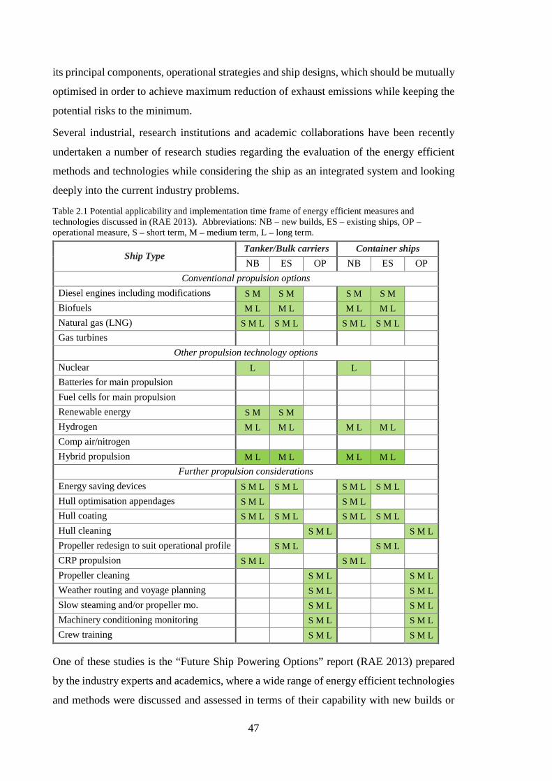
47
its principal components, operational strategies and ship designs, which should be mutually
optimised in order to achieve maximum reduction of exhaust emissions while keeping the
potential risks to the minimum.
Several industrial, research institutions and academic collaborations have been recently
undertaken a number of research studies regarding the evaluation of the energy efficient
methods and technologies while considering the ship as an integrated system and looking
deeply into the current industry problems.
Table 2.1 Potential applicability and implementation time frame of energy efficient measures and technologies discussed in (RAE 2013). Abbreviations: NB – new builds, ES – existing ships, OP – operational measure, S – short term, M – medium term, L – long term.
Ship Type Tanker/Bulk carriers Container ships NB ES OP NB ES OP
Conventional propulsion options Diesel engines including modifications S M S M S M S M Biofuels M L M L M L M L Natural gas (LNG) S M L S M L S M L S M L Gas turbines
Other propulsion technology options Nuclear L L Batteries for main propulsion Fuel cells for main propulsion Renewable energy S M S M Hydrogen M L M L M L M L Comp air/nitrogen Hybrid propulsion M L M L M L M L
Further propulsion considerations Energy saving devices S M L S M L S M L S M L Hull optimisation appendages S M L S M L Hull coating S M L S M L S M L S M L Hull cleaning S M L S M L Propeller redesign to suit operational profile S M L S M L CRP propulsion S M L S M L Propeller cleaning S M L S M L Weather routing and voyage planning S M L S M L Slow steaming and/or propeller mo. S M L S M L Machinery conditioning monitoring S M L S M L Crew training S M L S M L
One of these studies is the “Future Ship Powering Options” report (RAE 2013) prepared
by the industry experts and academics, where a wide range of energy efficient technologies
and methods were discussed and assessed in terms of their capability with new builds or

48
retrofitting while being allocated over the implementation time frame, namely, short,
medium and long terms as shown in Table 2.1 by the example of bulk carriers/tankers and
container ships.
Another key project, the scenario planning model for global shipping, GloTram, has been
developed as a part of the Low Carbon Shipping Consortium (Smith, Day, et al. 2014). The
model analyses the evolution of the global fleet in response to external factors including
fuel prices, transport demand, technology availability, cost and technical capability. In
other words, GloTram is aimed to quantify the drivers of the global shipping system, their
mutual interactions and explore potential future scenarios for the shipping industry. The
model’s outputs include the outlook of the future fleet size, costs revenues, future carbon
emissions level as well as the potential market share of energy efficient technologies and
marine fuels. Additionally, the decision-making process allows determining technical and
operational recommendations for new build or existing ships aiming to maximise the ship
owners profit and comply with environmental regulations.
To have a clear picture of the effect that could be achieved by efficiency improvements
using technical developments and innovations, it is essential to analyse, implement and
evaluate technical solutions for new and existing ships. As such, the Green Ship of the
Future, an open private-public partnership of the Danish maritime community with the
support of more than 40 global maritime industry parties, has been established in order to
explore, develop and demonstrate ambitious technical methods for cleaner, efficient and
sustainable ships and maritime operations. The project conducted a number of case studies
involving existing ship designs. One of their study (Klimt-Møllenbach et al. 2012) is
focusing on the 38,500 DWT tanker, being a similar ship to the tanker used in this PhD
research, while aiming to analyse the effect and costs of the most realistic alternatives to
the heavy fuel oil (HFO), namely low sulphur, LNG and scrubber technology, in order to
comply with the IMOs sulphur level regulations in emissions control areas (ECA). In fact,
this PhD research aims and objectives are extending the (Klimt-Møllenbach et al. 2012)
project as it focuses on the reductions of carbon emissions and therefore analyses an
additional set of technologies and methods, helping to create a complete picture of the
potential benefits from the energy efficient design and operational principals for this type
of ship.
Many of the energy efficient technologies are not applicable to all ship types nor are they
complementing each other or may even cause some damage and safety issues onboard. For
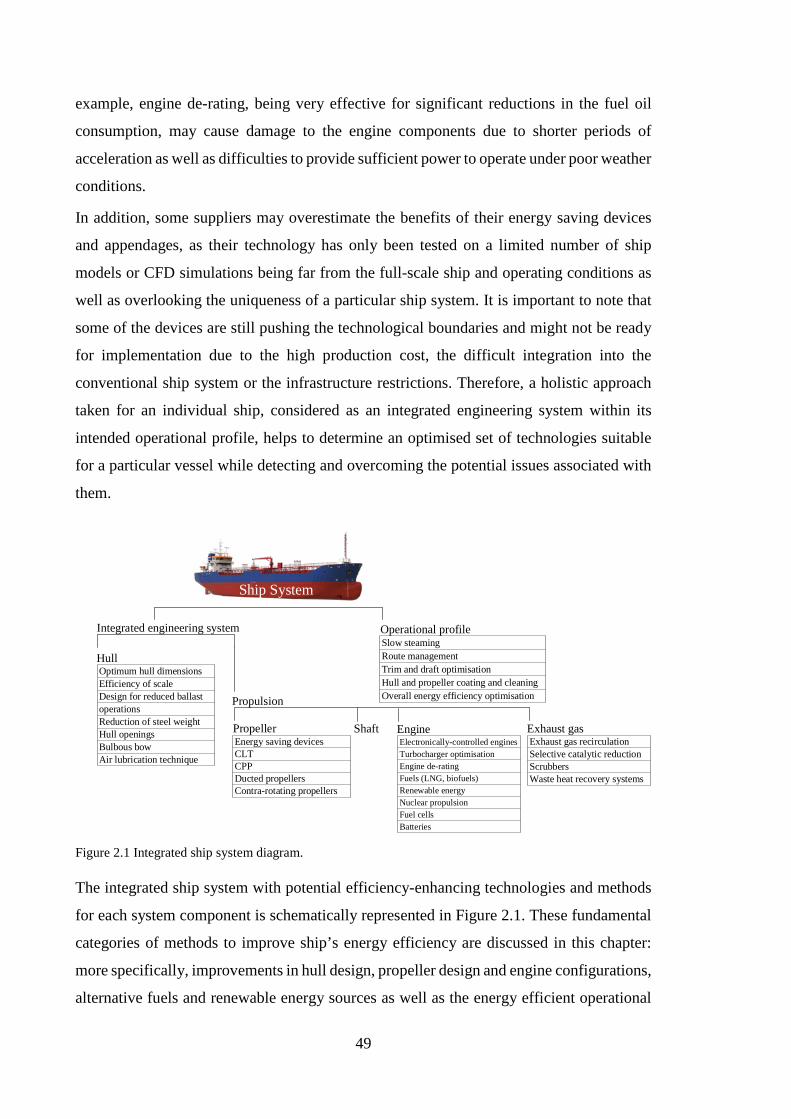
49
example, engine de-rating, being very effective for significant reductions in the fuel oil
consumption, may cause damage to the engine components due to shorter periods of
acceleration as well as difficulties to provide sufficient power to operate under poor weather
conditions.
In addition, some suppliers may overestimate the benefits of their energy saving devices
and appendages, as their technology has only been tested on a limited number of ship
models or CFD simulations being far from the full-scale ship and operating conditions as
well as overlooking the uniqueness of a particular ship system. It is important to note that
some of the devices are still pushing the technological boundaries and might not be ready
for implementation due to the high production cost, the difficult integration into the
conventional ship system or the infrastructure restrictions. Therefore, a holistic approach
taken for an individual ship, considered as an integrated engineering system within its
intended operational profile, helps to determine an optimised set of technologies suitable
for a particular vessel while detecting and overcoming the potential issues associated with
them.
Integrated engineering system Operational profile
Ship System
Slow steamingRoute managementTrim and draft optimisationHull and propeller coating and cleaningOverall energy efficiency optimisationPropulsion
HullOptimum hull dimensionsEfficiency of scaleDesign for reduced ballast operationsReduction of steel weightHull openingsBulbous bowAir lubrication technique
PropellerEnergy saving devicesCLT CPPDucted propellersContra-rotating propellers
EngineElectronically-controlled enginesTurbocharger optimisationEngine de-ratingFuels (LNG, biofuels)Renewable energyNuclear propulsionFuel cellsBatteries
Exhaust gas Exhaust gas recirculationSelective catalytic reductionScrubbersWaste heat recovery systems
Shaft
Figure 2.1 Integrated ship system diagram.
The integrated ship system with potential efficiency-enhancing technologies and methods
for each system component is schematically represented in Figure 2.1. These fundamental
categories of methods to improve ship’s energy efficiency are discussed in this chapter:
more specifically, improvements in hull design, propeller design and engine configurations,
alternative fuels and renewable energy sources as well as the energy efficient operational
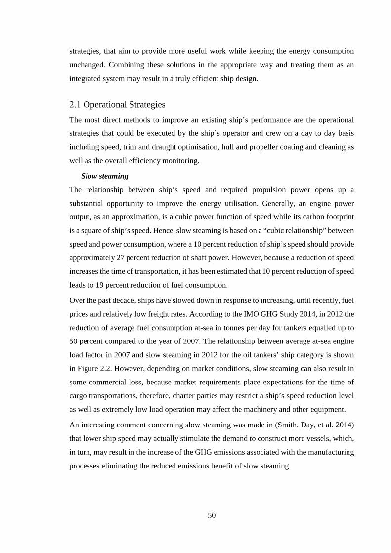
50
strategies, that aim to provide more useful work while keeping the energy consumption
unchanged. Combining these solutions in the appropriate way and treating them as an
integrated system may result in a truly efficient ship design.
Operational Strategies The most direct methods to improve an existing ship’s performance are the operational
strategies that could be executed by the ship’s operator and crew on a day to day basis
including speed, trim and draught optimisation, hull and propeller coating and cleaning as
well as the overall efficiency monitoring.
Slow steaming
The relationship between ship’s speed and required propulsion power opens up a
substantial opportunity to improve the energy utilisation. Generally, an engine power
output, as an approximation, is a cubic power function of speed while its carbon footprint
is a square of ship’s speed. Hence, slow steaming is based on a “cubic relationship” between
speed and power consumption, where a 10 percent reduction of ship’s speed should provide
approximately 27 percent reduction of shaft power. However, because a reduction of speed
increases the time of transportation, it has been estimated that 10 percent reduction of speed
leads to 19 percent reduction of fuel consumption.
Over the past decade, ships have slowed down in response to increasing, until recently, fuel
prices and relatively low freight rates. According to the IMO GHG Study 2014, in 2012 the
reduction of average fuel consumption at-sea in tonnes per day for tankers equalled up to
50 percent compared to the year of 2007. The relationship between average at-sea engine
load factor in 2007 and slow steaming in 2012 for the oil tankers’ ship category is shown
in Figure 2.2. However, depending on market conditions, slow steaming can also result in
some commercial loss, because market requirements place expectations for the time of
cargo transportations, therefore, charter parties may restrict a ship’s speed reduction level
as well as extremely low load operation may affect the machinery and other equipment.
An interesting comment concerning slow steaming was made in (Smith, Day, et al. 2014)
that lower ship speed may actually stimulate the demand to construct more vessels, which,
in turn, may result in the increase of the GHG emissions associated with the manufacturing
processes eliminating the reduced emissions benefit of slow steaming.
51
Figure 2.2 Average at-sea main engine load factor for oil tankers in 2007 – 2012.
This matter has also been discussed in (Tsimplis et al. 2012) concluding that a speed
reduction of 𝑥𝑥% requires a 1/(1 − 𝑥𝑥%) larger fleet to achieve the same transport
performance and provides equation 2.1 for estimating the increasing demand in ships under
slow steaming conditions:
𝑆𝑆𝑆𝑆𝑆𝑆 = 𝑆𝑆 ∗ 𝐷𝐷𝐵𝐵𝑆𝑆
1 − ∆𝑆𝑆 + (365 − 𝐷𝐷𝐵𝐵𝑆𝑆)
365 2.1
Where:
𝑆𝑆 and 𝑆𝑆𝑆𝑆𝑆𝑆 - the number of vessels of ship type and size category in the fleet at
normal speed and when slow steaming respectively
𝐷𝐷𝐵𝐵𝑆𝑆 - days at sea per year for ship type and size category
∆𝑆𝑆 - speed reduction as percentage of the baseline speed
In addition, since slow steaming is achieved by operating the main and axillary engines at
loads often below standard manufacturer recommendations for long periods, there is a risk
of an accelerated wear of the machinery components. Moreover, in the case of loads lower
than 40 percent of MCR running for a long time, some additional adjustments should be
made in order to prevent soot deposits in the exhaust gas boiler, soot build-ups in the
0 20 40 60 80 100
0 - 4,999
5,000 - 9,999
10,000 - 19,999
20,000 - 59,999
60,000 - 79,999
80,000 - 119,999
120,00 - 199,999
200,000 - +
% MCR
DW
T
2007 2012
52
turbocharger, increased heat load on components as well as excessive lube oil consumption.
However, these negative effects can be diminished by special fuel valves, exhaust gas boiler
bypass, reductions in cylinder oil feed rate, decreasing the turbocharger cleaning interval
and adding cut-out valves (ABS 2013). Additionally, electronically controlled engines are
designed to conform and may operate at lower loads.
Finally, the main engine’s specific fuel oil consumption (SFOC) is actually increasing up
to 10 percent at very low load operations, this being a function of the engine characteristics,
engine age and ship type. Therefore, this should be taken into account in the economic
assessment of slow steaming options and potential fuel savings.
Route management
Due to prevailing currents, wave heights, winds and weather patterns, the shortest Great
Circle distance between two points is not necessarily the fastest or the most fuel-efficient,
mainly because the maintenance of speed in poor weather increases the added resistance,
which, in turn, affects the fuel consumption. Alternatively, the reduction of ship’s speed in
adverse weather conditions causes delays in the transportation schedule. Therefore, weather
routing became essential in voyage performance management and aims to predict the
optimum speed with reduced fuel consumption while ensuring the safety of the crew,
passengers and the cargo.
Nowadays, weather and sea condition monitoring systems combined with navigational
software can contribute to approximately 10 percent fuel savings (Crist 2009). Such
systems are equipped with the real-time weather forecast data receivers and able to select
an optimal route with calmer sea conditions. Therefore, weather routing is a service
provided to the operator by a company which specialises in gathering and interpreting
metocean data to identify wind and sea condition and, finally, to estimate ship system
behaviour during its voyage using either a generic simulation model that matches ship’s
type and size or real geometric characteristics of the examinee ship. Such a ship behaviour
prediction simulation model is based on the model test data, empirical methods, full-scale
measurements or a real-time calculation of ship motions and added resistance.
The meteorological data processing is based on the mathematical modelling of the
atmosphere and weather system supplemented with the ocean wave forecasting models
based on the wind and the ocean current. In turn, the routing process is based on the
simulation of the various routes considering estimated weather conditions and safety limits.
In fact, weather routing is the most beneficial during longer voyages allowing to choose

53
from a wider range of possible routes as well as when the weather factor has a greater
influence on the fuel consumption.
Trim and draught optimisation
Since the hull forms are normally designed for a limited number of draughts (normally 1 –
3 draught levels such as ballast, design and laden) and often with no trim considered, when
in service, even small changes of trim may result in significant increase of ship’s resistance
and, therefore, negatively affect the fuel consumption. In fact, poorly optimised trim at low
load conditions may result in higher fuel consumption than in the case of a fully loaded
ship at proper trim. Therefore, it is vital for the operator to ensure a proper distribution of
the ballast and cargo while taking into account a specific combination of draught and trim
to minimise the power requirements. This is in addition to maintaining adequate margin
against the shear forces and bending moment acting on the hull.
In order to satisfy such demand, a number of trim optimisation tools have been developed.
Such tools are, normally, onboard software applications that estimate most favourable trim
conditions for the required draught as well as optimising the distribution of cargo or ballast.
The effectiveness of these trim optimisation tools, to a large extent, depends on the
estimation methods which could be classified as theoretical calculations/testing and real-
time measurements.
Normally, the estimation procedure of an optimum trim is based on model test data under
calm weather conditions where the resistance is estimated for a number of draught and trim
combinations generating a set of curves that indicate changes in resistance in accordance
with the required trim. This matrix is then incorporated into the onboard trim optimisation
tool. In fact, larger scale models provide more accurate predictions as they better match the
full-scale ship performance. However, large models require significant investments. In
addition, self-propulsion tests are also important to perform at the design stage as it helps
to detect sensitivity of the wake fraction and thrust deduction with changing trim and
draught, which are, generally, small but may have a significant impact on the propulsion
power demand.
Also, with the constantly increasing pace of technological development, a computational
fluid dynamics (CFD) approach is gaining more attention for trim optimisation purposes
being able to fairly correctly predict even small changes in resistance.
As such, the alternative method to overcome the uncertainty of calm weather predictions is
to integrate real-time on-board measurements for optimum trim estimations, which include

54
ship system performance under the corresponding draught and trim data harvesting in order
to generate the optimum trim tables. However, this method also has gaps in accuracy
associated with the difficulties in the elimination of the realistic trim/draught impact on the
power consumption from the other contributing components.
Hull and propeller coating and cleaning
The condition of the hull surface and its level of roughness may have a significant effect
on a ship’s performance. These factors may influence the scale of the boundary layer, thus
leading to an increase of the frictional resistance component when poorly maintained.
A hull surface roughness mainly depends upon two factors: permanent roughness, which
includes mechanical damage of the steel plates, corrosion or construction deficiencies; and
temporary roughness, often referred to marine biological fouling, but also influenced by
coating damage, coating deterioration or rough coating application and inaccurate polishing
of the surface before hull coating.
Marine biological fouling caused by spreading of living organisms over the wetted surface
includes bacteria, diatoms, algae, weed or even barnacles and mussels. The spread of
marine bacteria on a non-toxic hull surface has been described in many recent studies as
immediate, with the population reaching several thousand within few hours and several
million within two to three days. The primary slime film of 10 μm to 20 μm formed in early
stages of hull surface colonisation by the mixture of bacteria, diatoms and algae may
increase the total resistance by 1 percent for full-form ships and by 0.5 percent for fine-
form ships at high speeds.
The prevention of hull fouling lies with the performance of the hull coating. At present, the
main types of anti-fouling paints include Controlled Depletion Polymer (CDP), Self-
Polishing Copolymer (SPC) and silicone or fluoropolymer based Foul-Release Coatings.
All these coatings offer distinct levels of fouling protection, average hull roughness (AHR)
and lifetime. However, since CDP and SPC paints are based on the slow release of toxic
chemicals, biocides, they become depleted and require replacement after some years. The
main properties of these coatings are briefly described in Table 2.2. In fact, slow steaming
operation increases a risk of biological fouling making it difficult to keep the surface
smooth even for the most advanced coatings.
Despite the fouling protection and the level of smoothness, another valuable property of
antifouling hull paints is the ability to maintain its original state without often recoating.
This can be achieved through the proper monitoring and regular cleaning of the wetted
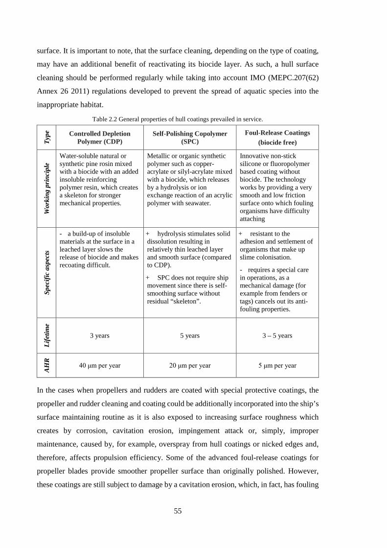
55
surface. It is important to note, that the surface cleaning, depending on the type of coating,
may have an additional benefit of reactivating its biocide layer. As such, a hull surface
cleaning should be performed regularly while taking into account IMO (MEPC.207(62)
Annex 26 2011) regulations developed to prevent the spread of aquatic species into the
inappropriate habitat.
Table 2.2 General properties of hull coatings prevailed in service.
Type
Controlled Depletion Polymer (CDP)
Self-Polishing Copolymer (SPC)
Foul-Release Coatings (biocide free)
Wor
king
prin
cipl
e
Water-soluble natural or synthetic pine rosin mixed with a biocide with an added insoluble reinforcing polymer resin, which creates a skeleton for stronger mechanical properties.
Metallic or organic synthetic polymer such as copper-acrylate or silyl-acrylate mixed with a biocide, which releases by a hydrolysis or ion exchange reaction of an acrylic polymer with seawater.
Innovative non-stick silicone or fluoropolymer based coating without biocide. The technology works by providing a very smooth and low friction surface onto which fouling organisms have difficulty attaching
Spec
ific
aspe
cts
- a build-up of insoluble materials at the surface in a leached layer slows the release of biocide and makes recoating difficult.
+ hydrolysis stimulates solid dissolution resulting in relatively thin leached layer and smooth surface (compared to CDP).
+ SPC does not require ship movement since there is self-smoothing surface without residual “skeleton”.
+ resistant to the adhesion and settlement of organisms that make up slime colonisation.
- requires a special care in operations, as a mechanical damage (for example from fenders or tags) cancels out its anti-fouling properties.
Life
time
3 years 5 years 3 – 5 years
AH
R
40 μm per year 20 μm per year 5 μm per year
In the cases when propellers and rudders are coated with special protective coatings, the
propeller and rudder cleaning and coating could be additionally incorporated into the ship’s
surface maintaining routine as it is also exposed to increasing surface roughness which
creates by corrosion, cavitation erosion, impingement attack or, simply, improper
maintenance, caused by, for example, overspray from hull coatings or nicked edges and,
therefore, affects propulsion efficiency. Some of the advanced foul-release coatings for
propeller blades provide smoother propeller surface than originally polished. However,
these coatings are still subject to damage by a cavitation erosion, which, in fact, has fouling
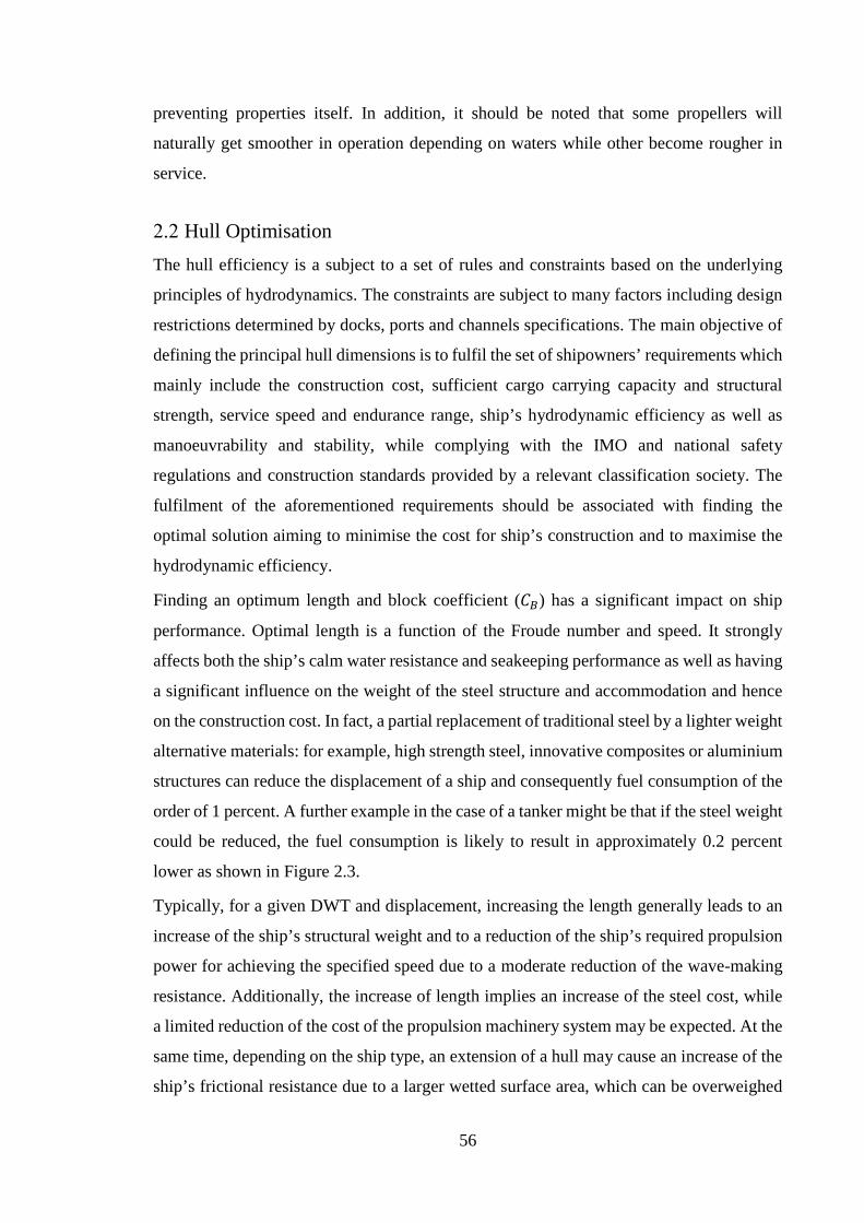
56
preventing properties itself. In addition, it should be noted that some propellers will
naturally get smoother in operation depending on waters while other become rougher in
service.
Hull Optimisation The hull efficiency is a subject to a set of rules and constraints based on the underlying
principles of hydrodynamics. The constraints are subject to many factors including design
restrictions determined by docks, ports and channels specifications. The main objective of
defining the principal hull dimensions is to fulfil the set of shipowners’ requirements which
mainly include the construction cost, sufficient cargo carrying capacity and structural
strength, service speed and endurance range, ship’s hydrodynamic efficiency as well as
manoeuvrability and stability, while complying with the IMO and national safety
regulations and construction standards provided by a relevant classification society. The
fulfilment of the aforementioned requirements should be associated with finding the
optimal solution aiming to minimise the cost for ship’s construction and to maximise the
hydrodynamic efficiency.
Finding an optimum length and block coefficient (𝐶𝐶𝐵𝐵) has a significant impact on ship
performance. Optimal length is a function of the Froude number and speed. It strongly
affects both the ship’s calm water resistance and seakeeping performance as well as having
a significant influence on the weight of the steel structure and accommodation and hence
on the construction cost. In fact, a partial replacement of traditional steel by a lighter weight
alternative materials: for example, high strength steel, innovative composites or aluminium
structures can reduce the displacement of a ship and consequently fuel consumption of the
order of 1 percent. A further example in the case of a tanker might be that if the steel weight
could be reduced, the fuel consumption is likely to result in approximately 0.2 percent
lower as shown in Figure 2.3.
Typically, for a given DWT and displacement, increasing the length generally leads to an
increase of the ship’s structural weight and to a reduction of the ship’s required propulsion
power for achieving the specified speed due to a moderate reduction of the wave-making
resistance. Additionally, the increase of length implies an increase of the steel cost, while
a limited reduction of the cost of the propulsion machinery system may be expected. At the
same time, depending on the ship type, an extension of a hull may cause an increase of the
ship’s frictional resistance due to a larger wetted surface area, which can be overweighed
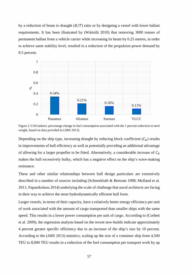
57
by a reduction of beam to draught (𝐵𝐵/𝑃𝑃) ratio or by designing a vessel with lower ballast
requirements. It has been illustrated by (Wärtsilä 2010) that removing 3000 tonnes of
permanent ballast from a vehicle carrier while increasing its beam by 0.25 metres, in order
to achieve same stability level, resulted in a reduction of the propulsion power demand by
8.5 percent.
Figure 2.3 Oil tankers: percentage change in fuel consumption associated with the 1 percent reduction in steel weight, based on data provided in (ABS 2013).
Depending on the ship type, increasing draught by reducing block coefficient (𝐶𝐶𝐵𝐵) results
in improvements of hull efficiency as well as potentially providing an additional advantage
of allowing for a larger propeller to be fitted. Alternatively, a considerable increase of 𝐶𝐶𝐵𝐵
makes the hull excessively bulky, which has a negative effect on the ship’s wave-making
resistance.
These and other similar relationships between hull design particulars are extensively
described in a number of sources including (Schneekluth & Bertram 1998; Molland et al.
2011; Papanikolaou 2014) underlying the scale of challenge that naval architects are facing
in their way to achieve the most hydrodynamically efficient hull form.
Larger vessels, in terms of their capacity, have a relatively better energy efficiency per unit
of work associated with the amount of cargo transported than smaller ships with the same
speed. This results in a lower power consumption per unit of cargo. According to (Corbett
et al. 2009), the regression analysis based on the recent new-builds indicate approximately
4 percent greater specific efficiency due to an increase of the ship’s size by 10 percent.
According to the (ABS 2013) statistics, scaling up the size of a container ship from 4,500
TEU to 8,000 TEU results in a reduction of the fuel consumption per transport work by up
0.34%
0.21%0.16%
0.11%
0
0.2
0.4
0.6
0.8
1
Panamax Aframax Suemax VLCC
%
58
to 25 percent while an additional increase by 4,500 TEU (from 8,000 TEU) boosts the
overall transport efficiency by approximately 10 percent. As for July 2015, the world’s
largest containership is the Malta-flagged “Barzan” built by Hyundai Samho Heavy
Industries in South Korea. Launched in May 2015 by the United Arab Shipping Company,
the vessel is 400 meters long while having 18,800 TEU capacity. As reported by DNV GL,
she has the latest energy efficient technologies as well as “has been designed and
constructed with the vision of undertaking a quick and cost-efficient retrofit to LNG at a
later stage”. Moreover, Barzan’s EEDI value is approximately 50 percent lower than it is
required by 2025.
Table 2.3 Maximum allowable ship dimensions in canals and channels.
Route Maximum passing dimensions
Panama Canal
New Panamax (since 2014): 𝐿𝐿 < 366 m 𝐵𝐵 < 49 m 𝑃𝑃 < 15.2 m Capacity of containers 12,000 TEU
Suez Canal
𝐿𝐿 – no limit 𝐵𝐵 < 71.02 m 𝑃𝑃 < 10.67 m (concerning stern draught in ballast condition) 𝑃𝑃 < 12.80 m (maximum allowable draught for 𝐵𝐵 <47.55 m, concerning fully loaded voyages southbound) 𝑃𝑃 < 16.15 m (maximum allowable draught for 𝐵𝐵 <42.67 m, concerning fully loaded voyages northbound)
Canal St. Lorenz (linking the inland Great Lakes of North America with the Atlantic Ocean)
𝐿𝐿 < 225.6 m 𝐵𝐵 < 23.8 m 𝑃𝑃 < 8.1 m
Northeast Sea Channel (Nord-Ostseekanal – Northern Europe)
𝐿𝐿 < 315 m 𝐵𝐵 < 40 m 𝑃𝑃 < 9.5 m
Malacca Straits (between Malaysia Peninsular and Sumatra island) 𝑃𝑃 < 25 m
However, the main ship dimensions such as length (𝐿𝐿), beam (𝐵𝐵), draught (𝑃𝑃) and capacity
are often affected by the topological limits of the route, namely, the dimensions of ports,
channels and canals that the projected ship needs to pass through. Some typical maximum
allowable ship dimensions of the most recognised canals and channels are listed in Table
2.3. In some cases, the ship length may also be restricted by the length of slipways or docks

59
of selected shipyards, with which the shipowner has a long-term collaboration in building
the new vessels and/or the maintenance of his fleet.
Additional efficiency savings may be achieved by incorporating the hull-enhancing
appendages. Perhaps, the most well-known among them is a bulbous bow. Generally, the
bulbous bow is applicable to a number of ship types with the waterline length longer than
about 15 meters that operate most of the time at or near its maximum speed. At lower
speeds, however, the bulbous bow may cause a minor gain in the frictional resistance due
to expanded, by its presence, wetted surface. Large ships, having relatively small changes
between loaded and ballast draughts with bulbous bow, would normally benefit by
approximately 10 percent in fuel efficiency in contrast to similar vessels without one.
Bulbous bows require a proper optimisation for gaining greater efficiency benefits. A set
of principal factors including the cross-sectional area at the forward perpendicular, volume,
vertical extension of the centre of volume as well as bulb section form and profile are
normally considered in bulbous bow design and optimisation process. For instance, a pear-
shaped bulbous bow is more efficient in combination with ballast or partially loaded
draughts while cylindrically shaped bulbs provide a compromise solution. Fuller ship
forms, normally tankers and bulk carriers, are often designed with bulbous bows that have
a large sectional area and a V-shaped transition of the bulb into the hull, which helps to
extend the waterline length at ballast conditions while traditionally acting when fully
loaded.
The added resistance due to turbulence, caused by the interrupted water flow around bow
thrusters tunnels or sea chest openings, can reach up to 2 percent of calm water resistance.
In order to reduce a negative effect of a pressure variation across the bow thruster tunnel,
the anti-suction tunnels can be additionally incorporated. It is also important to ensure that
the hull openings are properly faired so as to avoid any undue turbulence in flow along the
hull resulting from the discontinuity in the hull surface. At higher ship speeds, typically
above 25 knots, the use of actuating doors at the tunnel exits will minimise the ship
resistance penalty and noise emissions.
Possibly the most innovative hull-enhancing technology is the air lubrication technique.
The general idea is to cover the bottom of the ship with fine air bubbles, acting as a lubricant
which separates the hull’s wetted surface from water and, therefore, reduces frictional
resistance. For example, Mitsubishi Air Lubrication System (MALS), suitable for large
heavy cargo and passenger ships, claims to reduce fuel consumption by up to 10 percent

60
(Kawabuchi et al. 2011). At the same time, Maersk recently deployed a prototype of the air
lubrication system on one of their vessels, namely Olivia Maersk, aiming to verify the
potential energy efficiency benefits. The results did not prove the expected benefits. This
is because it was difficult to maintain the micro-bubbles size at full scale as they tend to
merge which significantly reduces the frictional resistance benefits.
Besides the resistance and propulsion performance, during the design process a proper care
should be taken regarding the stability, strength and manoeuvrability of a vessel while
meeting its desired operational profile. In addition, a hull design process should be
inseparably associated with the propeller design and engine matching underlining the
importance of the holistic system approach in ship hydrodynamic design.
Propellers and Energy Saving Devices The overall ship efficiency performance is strongly influenced by the type and
configuration of its propulsion system. The most commonly used propulsor types are the
fixed pitch propellers (FP), followed by the controllable pitch propellers (CP) (about 35
percent of the market) and ducted propellers (about 25 percent of the market), which, in
turn, can be equipped with either FP or CP propellers.
Fixed pitch propeller
In the case of fixed pitch propellers, an open water efficiency is normally expected to range
from approximately 50 percent for tankers and bulk carriers up to 75 percent for high speed
and slender vessels. Moreover, there are several options available for designers to enhance
the open water efficiency while controlling unwanted cavitation excitation and erosion on
the propeller blades. One of them is an introduction of the modified blade tip propeller
geometry, commonly known as the Contracted and Loaded Tip (CLT) propeller featuring
a blade end-plate technology. Another option for this type is the Kappel propeller. The core
idea is to reduce the tip vortex while obtaining a higher circulation towards the blade tips.
The working principle of these designs is similar to that of winglets at the end of aeroplane
wings. However, while a system such as a CLT propeller is claimed to significantly
improve an overall propulsion efficiency, the additional blade end-plates are increasing the
wetted surface of the propeller disk and, thus, causing extra frictional resistance.
Additionally, it is important to set the end plates at the correct attitude in relation to the
slipstream flow to prevent undue drag characteristics.

61
Another method to influence the open water efficiency is the reduction of rotational speed
(RPM) while allowing the diameter to increase at its optimum dimensions. However, there
are some design constraints which limit the scale of change including the hull and baseline
clearances, insufficient immersion as well as an increasing hull pressure and propeller
weight. Therefore, it is important to find an optimum balance to satisfy these constraints
while achieving the best performance of the propeller/engine combination.
Generally, with an increase of the propeller-specific loading, there is a growing risk of
cavitation erosion, predominantly caused by the pressure field in the flow (Bertram 2012),
which requires an additional expansion of the propeller’s blade area. On the other end of
the spectrum, there is a potential to increase the propeller efficiency through reduction of
the blade area, commonly expressed as a blade area ratio, which decreases frictional losses
associated with a larger wetted surface. However, any blade area reduction should be
consistent with the thrust loading requirements of the propeller from the cavitation point of
view.
The common way for preliminary estimation of the optimum blade area ratio while keeping
the global and harmful effects of cavitation under control is to undertake either Burrill’s or
Keller’s analysis procedure, both described in (Carlton 2012). The Keller’s method is based
on the empirical equations, while the Burrill’s procedure provides a cavitation diagram
based on model tests with a set of curves relating to back sheet cavitation extents applicable
to the uniform flow. These curves demonstrate the relationship between thrust loading
coefficient and the local cavitation number.
Thus, it is important to better understand the cavitation margins in relation to the blade area
ratio and propeller section design as well as to evaluate the potential efficiency benefits
associated with the reduction of the blade area ratio. This will help to find an optimum
balance between these factors. In addition, with growing industry interest in the research
and development of innovative propeller materials and coatings, the possibility for further
modification of the blade area ratio to achieve a better performance with a lower risk of
cavitation may substantially increase.
Controllable pitch propellers
Unlike fixed pitch propellers whose only operational variable is the rotational speed; the
controllable pitch propeller provides an additional possibility to adjust blade pitch. This is
particularly useful when a ship has two or more distinct operating conditions: for example
free running/trawling, anchor handling, day and night ferry services and so on.
62
Controllable pitch propellers are especially beneficial for ship manoeuvrability and the
applications involving shaft-driven generators, which require to keep the rotational speed
constant while managing the power absorption by changing the propeller pitch. The
controllable pitch propeller type is mostly preferred for the tags, passenger, ferry and
general cargo ship types.
When operating in off-design conditions under constant rotational speed, the overall
propeller efficiency performance of CPP might be lower compared to the conventional
FPP. This is because when operating at a constant rotational speed in off-design conditions,
the efficiency may fall off because the hydrodynamic conditions no longer relate to the
propeller design point. This also extends to the cavitation environment in which the
propeller operates since at off-design conditions there can be a tendency to develop face
cavitation as supposed to back cavitation in same conditions as well as to potentially
increase the level of vibration and noise. Conversely, CP propellers can be operated under
combinator-control where blade pitch and shaft RPM are varied simultaneously, which may
provide a slightly enhanced propeller efficiency and a more benign cavitation environment.
Alternatively, CPPs provide considerable benefits when the vessel is required to operate
under changing conditions such as manoeuvring or dynamic positioning situations.
Ducted propellers
Ducted propulsion system represents a propeller operating inside an annular duct. Since the
cross section of the nozzle has an aerofoil profile, it could have accelerating or decelerating
properties depending on its hydrodynamic profile. The latter one is commonly used to
manage cavitation and rarely, if at all, applied in large merchant vessels. Accelerating ducts,
often referred as Kort nozzles, are widely used for vessels with a high propeller-power
coefficient (𝐵𝐵𝑃𝑃), commonly tankers, bulk carriers, offshore service vessels, trawlers, tugs
and anchor handlers. The aim of the accelerating duct is to enhance the propulsion
efficiency by generating a lift on the duct by accelerating the inflow around the duct surface
and, thus, creating an additional thrust, which is the actual component of the generated lift
force. However, with increasing ship speed the level of propulsion efficiency benefits due
to the accelerating duct may fall to relatively modest amounts. It is also possible for a duct
to give a negative contribution to the propulsor thrust at high advance speeds. Nevertheless,
as reported by (AEA Energy and Environment 2008), power savings of up to 5 percent can
be expected from the ducted propeller performance compared to an open propeller
depending on the operating conditions.
63
Contra-rotating propellers
The contra-rotating propeller concept implies a pair of propellers placed one behind other
while rotating in opposite directions, where the aft propeller is designed to share the
propulsive load and recover some of the rotational energy in the slipstream from the
forward propeller. In addition, such a design philosophy allows lower propeller blade
loading compared to a single propeller resulting in better efficiency, which in the case of a
single screw vessel, as outlined in (Wärtsilä 2010), can reach up to 10 – 15 percent.
Although the principle of contra-rotating propellers has been known since 1876 de Bay’s
contra-rotating propeller for the steam yacht Iolaire, it was not prevalent until Morgan’s
research in 1960 when the fundamental principles of design begun to be more fully
understood.
In marine applications of contra-rotating propellers, it is common for the aftermost
propeller to have a smaller diameter than the forward propeller. This helps to accommodate
the slipstream contraction effects. Likewise, in order to avoid vibration due to blade parsing
frequencies, the blade numbers of the forward and aft propellers are usually different. The
contra-rotating propellers have found a significant number of applications in smaller high-
speed vessels and boats with the rotational speed around 1500 – 2000 rpm as well as with
torpedoes in order to eliminate the torque reaction. The application for larger merchant
vessels is rather limited due to a mechanical complexity of the shafting system.
In recent times, a novel application of the contra-rotating principle has been developed by
ABB which comprises a conventional fixed or controllable pitch propeller used in
association with podded propulsor. In this configuration, the conventional propeller is
coupled to the shaft line while the podded propulsor, which replaces the rudder, rotates in
the opposite direction thereby regaining some of the otherwise lost slipstream energy.
Energy saving devices
Coupled with the propeller, the energy saving devices (ESD) are intended to increase the
propulsive efficiency of a ship characterised by the Quasi Propulsive Coefficient (QPC),
which is a function of hull efficiency (𝜂𝜂𝐻𝐻), relative-rotative efficiency (𝜂𝜂𝑅𝑅) and open water
efficiency (𝜂𝜂𝑂𝑂) and defined as follows:
𝑄𝑄𝑃𝑃𝐶𝐶 = 𝜂𝜂𝐻𝐻 ∗ 𝜂𝜂𝑅𝑅 ∗ 𝜂𝜂𝑂𝑂 2.2 Among these elements, the open water efficiency (𝜂𝜂𝑂𝑂) has the most substantial influence
on the overall propulsive efficiency. The open water efficiency of the propeller for a given
ship, by definition in (Molland et al. 2011), is a product of an ideal efficiency characterised

64
by axial momentum theory for a propeller with a finite number of blades, losses associated
with the fluid rotation caused by the propeller as well as losses due to blade friction drag.
Energy saving devices can be categorised as the devices operating before the propeller (pre-
swirl devices), devices at the propeller and the post-swirl devices. The pre-swirl devices
stimulate a reaction with the boundary layer at the stern of the ship to provide more
homogenised flow beneficial for the propeller performance. In turn, the post-swirl devices
and the devices located at the propeller are aimed to recover energy losses by modification
to the flow field and the slipstream of the propeller.
Pre-swirl devices
Generally, the pre-swirl devices are easier to integrate with the hull structure. The most
known pre-swirl devices are Schneekluth wake equalizing duct (WED), Mewis duct,
Grothues spoilers, flow conditioning ducts, pre-swirl fins and Grim vane wheel.
• Schneekluth wake equalizing duct (WED) The wake equalising duct (WED), initially proposed by Schneekluth, aims to reduce the
separation around the ship’s stern by redirecting the flow to the upper part of the propeller
while establishing a more homogenous wake field (Schneekluth & Bertram 1998). This
helps to enhance the hull and open water efficiencies by moderate reduction of the wake
fraction and thrust deduction coefficients. Moreover, WED may cause a generation of the
low-pressure areas in the front part of the duct which could provide additional efficiency
benefits by reattaching separated flow to the hull. However, in case the flow around the
stern is fine and uniform, such low-pressure regions may increase the thrust deduction
coefficient. According to the manufacturers, the guidance energy saving benefits of WED
amount up to 12 percent depending on the flow configurations and propeller thrust loading.
• Grothues spoilers Grothues spoilers (Grothues-Spork 1988) represent a hydrodynamic fin system, consisting
of small curved triangular plates fitted to the stern of the hull in front of the propeller disk
and above the propeller axis. The main idea of Grothues spoilers is to straighten the flow
directed towards the propeller due to the curved shape of fins helping to align the leading
edge of the fin with the surrounding flow direction thereby minimising the vorticity in the
incident flow field into the propeller. Ideally, spoilers may generate an additional thrust by
inclining the vertical flow in the horizontal direction.

65
The expected benefits from the application of such spoilers are strongly dependent upon
the correct adjustment of a curvature angle of each spoiler in line with the incoming flow
as well as positioning along the stern surface in order to prevent an additional friction.
• Flow conditioning ducts and pre-swirl fins The main purpose of the flow conditioning ducts is to bring uniformity to the propeller
inflow by the action of the duct, which is normally positioned ahead of the propeller. The
pre-swirl fins represent a simple system of fins located directly ahead of the propeller
around the shaft axis and designed to improve the propulsive efficiency through pre-
rotating the propeller inflow. When combined with the pre-swirl fins, the flow conditioning
ducts enhance the inflow to the stator which increases their efficiency.
There are several types of the flow conditioning duct systems available on market including
Mitsui integrated ducted propeller, Hitachi’s Zosen nozzle, Sumitomo’s Integrated
Lammeren duct and Mewis duct. As an example, the Mewis duct consists of a duct
positioned ahead of the propeller together with an integrated fin system within. It is claimed
to provide energy savings of 3 – 8 percent depending on the hull form. Mewis ducts were
tested and installed on medium sized ships ranging from 45,000 to 50,000 DWT with
reported reductions in propeller pressure pulses and tip cavitation (MER 2012).
• Grim vane wheel The Grim vane wheel is a freely rotating device located behind the propeller, namely on
the tail shaft or the rudder horn (Grim 1980). It aims to capture energy from the propeller
slipstream and convert this energy into an additional propulsive thrust. The vane wheel
consists of the turbine section inside the propeller slipstream and a propeller section outside
the propeller slipstream. Therefore, the diameter of the vane wheel is normally larger than
the actual propeller diameter while having a greater number of blades in comparison to the
original propeller.
Grim vane wheels are suitable for a wide range of conventional cargo ships and could
provide 7 – 10 percent in efficiency improvements (Breslin & Andersen 1994). However,
there are concerns that collisions with wood or ice floes may damage the vane wheel and
in some cases the bearing upon which the wheel sits. Therefore, since the system is
mechanically sensitive and involves considerable investment, only a few actual
installations have been reported (Bertram 2012).

66
Post-swirl devices
Alternatively, the post-swirl devices are designed to condition the post-propeller flow while
operating behind the propeller within its slipstream region and include a range of rudder
bulbs, fins, stators and other concepts as well as combinations of them.
• Rudder – bulb systems Rudder – bulb system is designed to prevent flow separation as well as excessive vorticity
behind the hub by successfully extending the propeller boss. Typically, the system
comprises a large bulb with the diameter of some 20 percent of the actual propeller
diameter. The bulb is placed on the rudder immediately behind the propeller boss. In some
cases, the system also incorporates a set of four fins located in an X – shape manner. Since
the fins operate in the helical slip – stream and, thus, receive the flow at incidence, they
produce a lift force, which acts in the forward direction and results in additional propulsive
thrust.
• Asymmetric rudder Asymmetric rudder system consists of two distinctive regions. The regions above and
below the propeller axis have aerofoil properties and both regions are optimised to work in
the wake field of the propeller. The system allows the effects of the rotation of the
propeller’s slipstream to be countered which results in the reduced drag. Other important
benefits are directed towards reducing rudder cavitation erosion and, hence, extending the
lifespan for the rudders and lowering the level of vibration and noise.
As stated in (Corbett et al. 2009), for these devices, a gain in propulsive efficiency vary
from 1 to 8 percent based on the model test results, whereas full-scale measurements are
only available for the combination of fins with rudder and estimated to be 8 – 9 percent.
Additionally, post-swirl devices are often combined with pre-swirl devices, which, in fact,
may reduce a contribution of the post-swirl devices into the overall efficiency due to pre-
swirl devices would already neutralise the post-rotational flow of the propeller. In addition,
a potential gain in energy efficiency from such devices is generally lower for optimal hull
and propeller designs as their initial purpose was to improve the flow around the hull in
order to eliminate energy losses due to poorly designed stern or propulsor. In the design of
these devices, it is important to endeavour to take into account the scaling effects from
model to full scale. In this contexts, the use of CFD methods can be helpful.
67
• Boss cap fins Some devices may be attached to the propeller hub to break up the hub vortex generated
behind the rotating propeller. The boss cap fin comprises a small vane propeller fixed to
the tip of a cone-shaped boss cap, which may have more blades than the propeller itself.
First developed and manufactured at the end of the 1980s in Japan, it has had over 2,000
installations worldwide with the manufacturer’s savings claims of 3-5 percent. However,
according to at-sea performance tests, their effectiveness was reduced at slower steaming
speeds.
It is important to emphasise that manufacturers often claim very promising figures of
reductions in fuel consumption, which seem to be very optimistic and require independent
research. Such evaluations have been conducted by (Smith, Day, et al. 2014) and included
several case studies of the hydrodynamic performance of vessels incorporated with WEDs,
a combination of WED and pre-swirl fins, a twisted rudder and propeller boss cap fins using
simplified CFD models. The obtained results have shown that in all cases the expected
benefits were lower than originally claimed.
Since it is difficult to discriminate the performance improvements below 3-4 percent, it can
be extremely difficult to justify efficiency claims for particular devices which claim the
benefits below this region. This is due to the statistical errors encountered in continuously
monitored data while bearing in mind the variabilities of machinery operations, signal
measurement and environmental conditions.
Machinery Improvements Since low-speed diesel engines are designated as the most efficient, diesel propelled
machinery became the most common choice for the marine propulsion of large merchant
vessels. At the current state of technology, the diesel engine fuel efficiency can reach up to
50 percent (MAN Diesel and Turbo 2014c). Therefore, only half of the fuel’s specific
energy is converted into the mechanical energy and can be directly transmitted to the
propeller. Medium speed diesel engines generally have 3 – 4 percent lower fuel efficiency.
In addition, they are normally connected to the propeller through the speed reduction
devices, commonly a reduction gear box or electric drive system, which induce additional
efficiency losses of about 2 - 3 percent in case of reduction gear and up to 8 percent when
an electric drive system is used (MAN Diesel and Turbo 2015). Such losses are reflected
in the fuel consumption to satisfy the ship’s power requirements. Low-speed diesel engines

68
are commonly used for main propulsion on large merchant vessels, especially tankers, bulk
carriers and container/general cargo ships, while medium speed diesel engines are generally
applied as a part of an auxiliary system of these ship types or as the main propulsion for
smaller commercial vessels, cruise ships, ferries and large fishing boats. In addition, LNG
carriers are normally equipped with steam, diesel-electric propulsion systems or dual fuel
slow speed engines.
With increasing demand for sustainable shipping, engine designers and manufacturers are
constantly striving to reduce exhaust emissions while improving fuel efficiency. Currently,
MAN, Wärtsilä, Rolls-Royce and Caterpillar are among the biggest engine market players
to satisfy the energy efficiency demand while complying with exhaust emissions
regulations by offering a vast portfolio of marine technologies and devices including dual
fuel engines that can operate on both, the fuel oil and natural gas.
Since enhanced efficiency can be achieved through the introduction of innovative
equipment or by improving engine’s operation philosophy, the following section is aimed
to discuss the most attractive innovative technologies and methods designed to enhance
fuel efficiency.
Electronically controlled engines
Many modern marine diesel engines are supported by a digital electronic control of fuel
injection quantity, fuel injection timing, exhaust valve timing and etc., which results in
approximately 2 – 2.5 percent reduction in SFOC at low and medium loads compared to
conventional engine performance (MAN Diesel and Turbo 2014b). Electronically
controlled low-speed diesel engines, referred as ME type in MAN and Flex type in
Wärtsilä, are also associated with a common rail technique, where the fuel is supplied by
high-pressure common rails equipped with solenoid valves and controlled by the electronic
system. This electronic system helps to optimise the fuel injection point in the
thermodynamic cycle in accordance with the required engine load and to maximise its
efficiency, while the exhaust valve control, allows variable timing to maximise scavenging
(Smith, Day, et al. 2014).
Engine control tuning is another innovative method available for low speed electronically
controlled engines, which is designed to control the exhaust valve timing and injection
profiling in order to reduce SFOC via the automatic adjustment of a maximum cylinder
pressure in accordance with the engine load. In fact, while for conventional low-speed
diesel engines the introduction of SFOC reduction methods via compression adjustments

69
may result in increased level of 𝑁𝑁𝐶𝐶𝑋𝑋 for low load operations and, thus, should be monitored
and balanced in accordance to IMO Tier II regulations; in the case of electronically
controlled engines, it is possible to reduce SFOC while keeping the 𝑁𝑁𝐶𝐶𝑋𝑋 level to its
minimum as required by Tier II compliance.
Turbocharger optimisation
For ships continuously operating under slow steaming conditions, turbocharger control
systems can be incorporated to reduce SFOC by 2 to 4 g/kWh. Examples of such systems
include the Variable Turbocharger Area (VTA) by MAN or Variable Turbine Geometry
(VTG) by Wärtsilä, both compatible with large-bore two- or four- stroke diesel and gas
engines with camshaft or electronically controlled system.
The idea is to adjust the nozzle ring of the turbocharger in accordance with the engine load
such as the nozzle ring is expanded with full load operation while narrowing down with the
decreasing load. As a result, SFOC at full load is higher while at partial or low load is
optimally reduced. In the case of multiple turbochargers installed, similar effects can be
achieved by cutting out one turbocharger unit.
Another method to enhance fuel efficiency at lower loads is the Exhaust Gas Bypass (EGB).
The system is optimised to work under the both, low and high loads. For the lower loads
operation, a smaller turbocharger system is used to provide the engine with its efficiency
demand. In the case of a full load operation, the exhaust gas is bypassed beyond the
turbocharger to prevent it from the over-speeding. An additional benefit from EGB system
is an increase of the exhaust gas temperature, resulting in the greater amount of steam at
the exhaust gas boiler. The most efficient utilisation of the bypass technology may be
achieved when used in combination with the common rail technology.
Engine de-rating
Another effective method of SFOC reduction is the engine de-rating. Thermodynamic
efficiency of an engine is defined by a relationship between the maximum burning pressure
and mean effective pressure (MEP). The engine de-rating means the operation of an engine
at its maximum cylinder pressure for the design continuous service rating, but at a lower
mean effective pressure and/or shaft speed. For example, a higher-power engine de-rated
to a lower Specific Maximum Continuous Rating (SMCR), while meeting the required
design performance of a ship, will develop lower MEP, which, therefore, will result in
lower SFOC at the operating design point.

70
For an existing ship and without changing the propeller, the engine de-rating will result in
a lower ship speed. In the case of newbuildings, the de-rated engine horsepower is that
which will drive the ship at a given speed with the propeller optimised to absorb this
horsepower at a lower than normal shaft speed. The optimisation would normally require
an installation of a more efficient propeller, a larger propeller diameter operating at its
optimum RPM, reduction of a blade area ratio or a larger stroke to bore ratio.
For newbuildings, it is also common to install the engine with the increased number of
cylinders. An extra expense associated with the additional cylinder would normally be paid
back in 3-4 years (MAN Diesel and Turbo 2014a). For example, if the ship’s required
propulsion power with an applied sea margin is 8300 kW at 127 RPM, a conventional
option is to choose an engine with the maximum installed MCR = 8300 kW at 127 RPM
(SMCR = MCR). In this case, MAN 5S50ME-C will perfectly suit the ship’s requirements.
In the case of de-rating, the same model of the engine at the same speed is selected but with
one additional cylinder, namely MAN 6S50ME-C with MCR = 9960 kW at 127 RPM, and
then de-rated to SMCR = 8300 kW at 127 RPM. The average reduction in SFOC under the
de-rated condition, as illustrated in Figure 2.4, will reach up to 3 percent, taking into
account additional losses due to increased friction of the extra cylinder and piston. In
addition, engine de-rating has a great influence on the EEDI measure as it allows to reduce
SFOC while keeping the power and ship speed unchanged.
Figure 2.4 SFOC behaviour comparison under conventional and de-rated conditions. Based on MAN CEAS engine calculations.
150
155
160
165
170
175
180
0 20 40 60 80 100 120
SFO
C g
/kW
h
Load %Original 5S50ME-C (MCR = SMCR = 8300 kW at 127 RPM)
De-rated 6S50ME-C (MCR = 9960 kW at 127 RPM, SMCR = 8300 kW at 127 RPM)

71
It should be emphasised that de-rating of an existing engine will require reducing ship’s
maximum speed, which should be considered with extra caution as the engine must provide
a sufficient power to operate under poor weather conditions or to manoeuvre in restricted
areas. Engine de-rating also increase a risk of accelerated wear of the machinery
components and may cause the engine inner damage due to shorter periods of acceleration.
Finally, uprating the de-rated engine back to its designed conditions in order to increase
ship’s speed is only possible if the auxiliary equipment supports a larger rating.
𝑵𝑵𝑵𝑵𝑿𝑿 control technologies
Since the MARPOL Annex VI Tier II and further Tier III requirements, aiming to reduce
the level of 𝑁𝑁𝐶𝐶𝑋𝑋 emissions, tend to negatively influence SFOC, there is an increasing
demand for alternative treatments that will keep both the 𝑁𝑁𝐶𝐶𝑋𝑋 level and SFOC to the
minimum.
Generally, the quantity of 𝑁𝑁𝐶𝐶𝑋𝑋 emissions is a function of combustion temperature, duration
of the combustion process and the quality of combustion. Therefore, primary methods of
𝑁𝑁𝐶𝐶𝑋𝑋 reduction are focused on a decrease of the combustion duration time and firing
temperature, control of fuel injection and the introduction of higher-pressure turbocharging
(RAE 2013), which resulted in extensive development of innovative turbocharging
technologies. For example, by means of two-stage turbocharging techniques the charge air
pressure can be increased substantially resulting in higher power density (if required) and,
in conjunction with Miller engine cycle, where the engine is compressing against the
pressure of the turbocharger rather than the pressure of the cylinder walls, reduced exhaust
emissions and lower fuel consumption.
Moreover, there is a range of alternative treatments for 𝑁𝑁𝐶𝐶𝑋𝑋 which are now commonly used
including the exhaust gas recirculation (EGR) and selective catalytic reduction (SCR).
As the name implies, exhaust gas recirculation system recirculates the exhaust gas flow to
the engine intake manifold for 𝑁𝑁𝐶𝐶𝑋𝑋 reduction purposes and is suitable for slow and medium
speed diesel engines. The effect of this system is derived from a slightly increased heat
capacity of the scavenge air where a minor part of the oxygen in the scavenge air is replaced
by carbon dioxide from the combustion. This also helps to reduce the temperature picks of
the combustion (Kristensen 2012). In fact, preliminary studies have shown that application
of EGR systems in terms of Tier III regulations may result in sufficient increase in SFOC
(1 – 2 g/kWh) compared to Tier II engines. An interesting example of the in-service
72
application of EGR system on-board of the Alexander Maersk, illustrated in (RAE 2013),
has shown a good performance and supported further idea of the EGR application.
The basic idea of a selective catalytic reduction (SCR) is to remove unwanted 𝑁𝑁𝐶𝐶𝑋𝑋
footprint from the exhaust gas via chemical reaction, which relies on the injection of
ammonia into the exhaust gas flow, usually in the form of a urea solution. This promotes a
chemical reaction with 𝑁𝑁𝐶𝐶𝑋𝑋 species at the surface of the selective catalytic reduction
system, leading to formation of nitrogen and steam. The SCR system, while not involving
significant modifications to the existing propulsion system, requires an additional space for
urea storage in the engine room. In case of low-speed diesel engines, the SCR system is
recommended to be installed between the turbocharger and the exhaust gas manifold,
providing higher exhaust gas temperatures for more efficient SCR reaction. However, this
may result in slight reduction of the overall engine efficiency as it negatively affects the
turbocharger. Alternatively, for medium speed diesel engines the SCR system should be
installed after the turbocharger. The SCR technology, according to (MAN Diesel and Turbo
n.d.), is capable to remove up to 95 percent of 𝑁𝑁𝐶𝐶𝑋𝑋 in the exhaust flow making it a
promising solution when operating in ECA areas. However, since it is usually a challenge
to find the required space for the catalyst, piping, support, auxiliary equipment as well as
𝑁𝑁𝐶𝐶𝑋𝑋, 𝐶𝐶2 and ammonia (𝑁𝑁𝐻𝐻3) measuring devices, it is far more complicated to retrofit the
installation than to integrate the SCR system into the newbuilding.
Scrubbers
With increasing concern and upcoming regulatory restrictions in emission control areas
(ECAs) regarding harmful environmental and health impact of sulphur content in marine
fuels, there is a continuing research and development of alternative methods, such as
exhaust gas after-treatment systems, that aimed to remove sulphur oxides from the exhaust
gas flow and can be used in addition to relatively expensive low sulphur fuels while keeping
conventional MDO and HFO as a primary option outside ECA.
Seawater scrubbing is one of them. The method involves utilisation of alkalines 𝐻𝐻𝐶𝐶𝐶𝐶3 and
𝑆𝑆𝐶𝐶4 present in sea water to neutralise 𝑆𝑆𝐶𝐶𝑋𝑋 species in the exhaust gas via a chemical
reaction. This reaction results in production of sulphates, which are being recirculated back
into the sea. Before the discharge, the sea water is also filtered to remove heavy metals and
particulate matter. Such systems have a relatively simple operating cycle and do not require
large amounts of waste storage and handling on board. However, there is an uncertainty on
the potential consequences of the sulphates-rich waste discharged after the exhaust gas

73
treatment and some ports and areas may not permit to discharge of the waste water
containing sulphur. Alternatively, since sea water already contains a relatively high amount
of sulphur, its impact on the marine environment is relatively low and IMO has already
approved this technology by adopting (MEPC.184(59) Annex 9 2010).
In fact, the effectiveness of sea water scrubbing systems decreases in some areas including
the northern part of the Baltic Sea and Alaska since the alkalinity level in those regions is
considerably lower. Therefore, in order to avoid such alkalinity issues, there is an
alternative to seawater scrubbers, namely freshwater scrubbers (or closed loop scrubbing
system) that additionally involve a caustic soda (𝑁𝑁𝐻𝐻𝐶𝐶𝐻𝐻) solution to neutralise the sulphur
in the marine exhaust. Most of the scrubbing agent is recirculated with only minimal water
intake and discharge. These systems are more complex and costly to exploit, while creating
waste storage and handling issues on board. A variation on the closed loop system is a
hybrid system which can operate as an open loop system while outside special control areas.
According to the analytical study conducted by (Boer & Hoen 2015), scrubbers reduce the
emission of sulphur to the atmosphere by more than 90 percent. In addition, scrubbing helps
to reduce PM (by mass) by 60-90 percent while the amount of 𝑁𝑁𝐶𝐶𝑋𝑋 can be reduced by up
to 10 percent. However, due to the extra power required to operate pumps and caustic soda
consumption, the estimated additional GHG emissions range between 1.5 and 3.5 percent,
while the consumption of additional MGO in the ECA causes a rise of GHG refinery
emissions by roughly 6.5 percent.
Since the scrubber technologies can be retrofitted into existing ships, the (Klimt-
Møllenbach et al. 2012) project, based on the existing tanker, undertook a case study of a
hybrid scrubbing system. This system is capable of operating on both, fresh water and sea
water while burning heavy fuel oil. The results have shown a necessity for a new funnel
layout due to the introduction of the scrubber together with relevant machinery and new
tanks. Moreover, the installation costs of the scrubbing system are estimated to be USD
5.84 million, whereas the cost of scrubbers and its relevant equipment amounted to USD
2.6 million.
Waste heat recovery system (WHRS)
Although the thermal efficiency of modern diesel engines is continuously improving with
the technological progress, a significant amount of waste heat is still being generated
especially when operating under high loads. Normally, the waste heat is utilised onboard
to produce fresh water or for accommodation heating purposes. However, with increasing
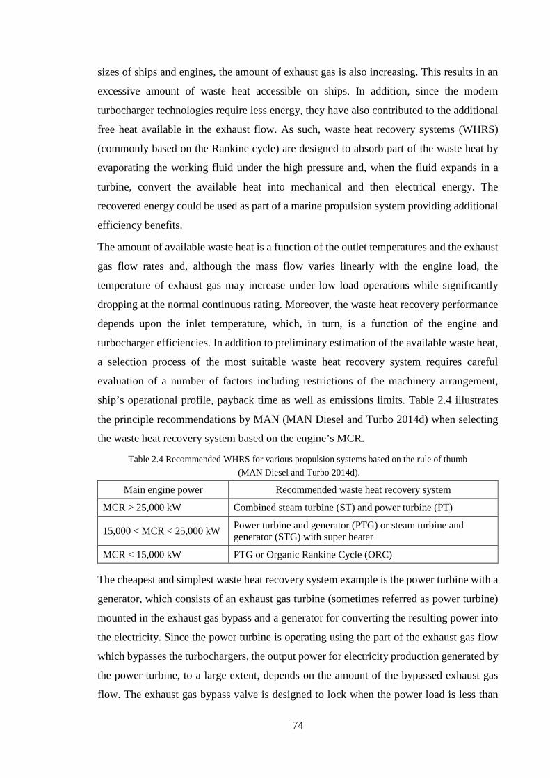
74
sizes of ships and engines, the amount of exhaust gas is also increasing. This results in an
excessive amount of waste heat accessible on ships. In addition, since the modern
turbocharger technologies require less energy, they have also contributed to the additional
free heat available in the exhaust flow. As such, waste heat recovery systems (WHRS)
(commonly based on the Rankine cycle) are designed to absorb part of the waste heat by
evaporating the working fluid under the high pressure and, when the fluid expands in a
turbine, convert the available heat into mechanical and then electrical energy. The
recovered energy could be used as part of a marine propulsion system providing additional
efficiency benefits.
The amount of available waste heat is a function of the outlet temperatures and the exhaust
gas flow rates and, although the mass flow varies linearly with the engine load, the
temperature of exhaust gas may increase under low load operations while significantly
dropping at the normal continuous rating. Moreover, the waste heat recovery performance
depends upon the inlet temperature, which, in turn, is a function of the engine and
turbocharger efficiencies. In addition to preliminary estimation of the available waste heat,
a selection process of the most suitable waste heat recovery system requires careful
evaluation of a number of factors including restrictions of the machinery arrangement,
ship’s operational profile, payback time as well as emissions limits. Table 2.4 illustrates
the principle recommendations by MAN (MAN Diesel and Turbo 2014d) when selecting
the waste heat recovery system based on the engine’s MCR.
Table 2.4 Recommended WHRS for various propulsion systems based on the rule of thumb (MAN Diesel and Turbo 2014d).
Main engine power Recommended waste heat recovery system
MCR > 25,000 kW Combined steam turbine (ST) and power turbine (PT)
15,000 < MCR < 25,000 kW Power turbine and generator (PTG) or steam turbine and generator (STG) with super heater
MCR < 15,000 kW PTG or Organic Rankine Cycle (ORC) The cheapest and simplest waste heat recovery system example is the power turbine with a
generator, which consists of an exhaust gas turbine (sometimes referred as power turbine)
mounted in the exhaust gas bypass and a generator for converting the resulting power into
the electricity. Since the power turbine is operating using the part of the exhaust gas flow
which bypasses the turbochargers, the output power for electricity production generated by
the power turbine, to a large extent, depends on the amount of the bypassed exhaust gas
flow. The exhaust gas bypass valve is designed to lock when the power load is less than

75
approximately 40 percent. As such, depending on the engine size, the power turbine and
generator based waste heat recovery system will provide up to 5 percent recovery ratio
(MAN Diesel and Turbo 2014d).
Another example of a waste heat recovery system is a steam turbine, where, to enhance the
heat to the boiler, the exhaust gas bypass flow is mixed with the stream from the
turbocharger. This results in increased exhaust gas temperature before the boiler inlet.
Therefore, the amount of potential steam production and, hence, the resulted power output
is greater compared to power turbine, which estimated to reach up to 8 percent depending
on the main engine size and ambient conditions.
In case of increased power demand, the power turbine can be used in conjunction with the
steam turbine connected via reduction gear boxes forming a joint system, such as the steam
turbine is specified to start first at 30 – 35 percent SMCR followed by the power turbine at
40 – 50 percent SMCR, which will result in up to 11 percent of recovered power.
The preferred working fluid used in a thermodynamic waste heat recovery system is water
since it provides high power outputs without chemical decomposition and extensive
condensation inside the turbine. However, it is possible to increase the power output as well
as the thermal efficiency using organic fluids (for example based on carbon molecules)
instead of water. For instance, the comparison study conducted by (Suarez et al. 2013)
aiming to compare the performance of water and a number of organic working fluids,
namely Heptane, Benzene, Toluene and Hexamethyldisiloxane in the Rankine cycle based
waste heat recovery system while operating 14 cylinders 87 MW 2-stroke diesel engine,
has shown that the maximum net power output (2,233 kW at a thermal efficiency of 22.1
percent) was delivered by benzene, while water-based Rankine cycle generated 1,987 kW
at 18.6 percent.
Alternative Ship Propulsion and Fuels According to recent figures by (IMO 2014b), the shipping industry on a global level
annually consumes approximately 330 million tonnes of fuel where 80 – 85 percent account
for residual fuel, commonly referred as a heavy fuel oil (HFO), with a high sulphur content.
Alternatively, ships engaged in coastal voyages and environmentally controlled areas, in
the majority of cases, burn lighter marine diesel oil (MDO) being a blend of gasoline and
heavy fuel oil. Since HFO is a residual product remaining at the end of the crude oil refining
chain, it contains a generous amount of impurities such as oxides, sulphur, and water (Crist
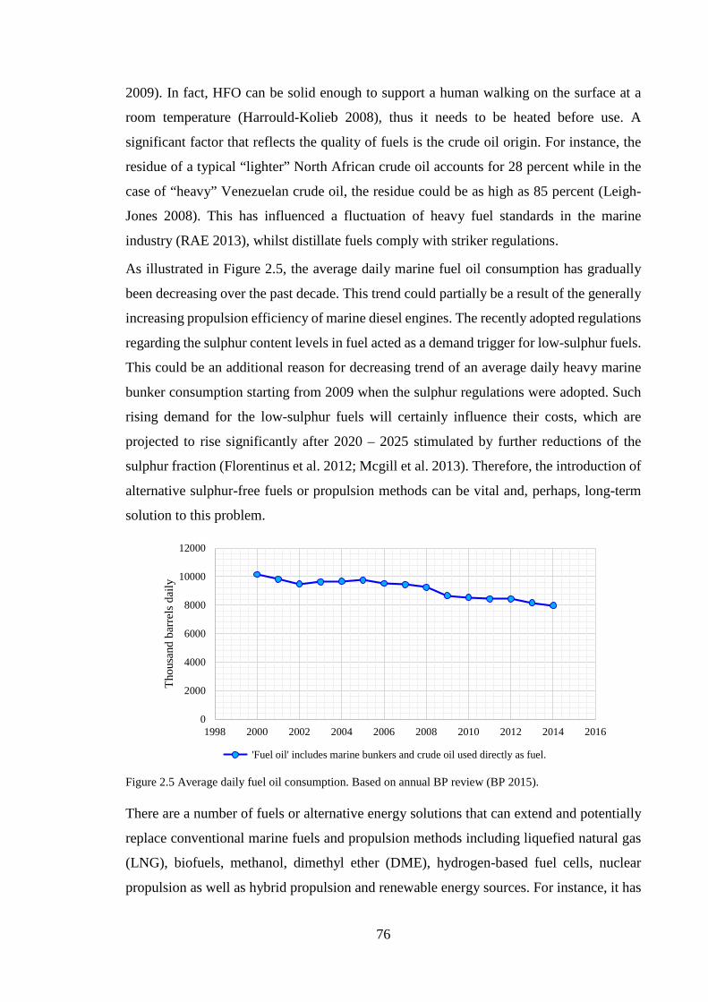
76
2009). In fact, HFO can be solid enough to support a human walking on the surface at a
room temperature (Harrould-Kolieb 2008), thus it needs to be heated before use. A
significant factor that reflects the quality of fuels is the crude oil origin. For instance, the
residue of a typical “lighter” North African crude oil accounts for 28 percent while in the
case of “heavy” Venezuelan crude oil, the residue could be as high as 85 percent (Leigh-
Jones 2008). This has influenced a fluctuation of heavy fuel standards in the marine
industry (RAE 2013), whilst distillate fuels comply with striker regulations.
As illustrated in Figure 2.5, the average daily marine fuel oil consumption has gradually
been decreasing over the past decade. This trend could partially be a result of the generally
increasing propulsion efficiency of marine diesel engines. The recently adopted regulations
regarding the sulphur content levels in fuel acted as a demand trigger for low-sulphur fuels.
This could be an additional reason for decreasing trend of an average daily heavy marine
bunker consumption starting from 2009 when the sulphur regulations were adopted. Such
rising demand for the low-sulphur fuels will certainly influence their costs, which are
projected to rise significantly after 2020 – 2025 stimulated by further reductions of the
sulphur fraction (Florentinus et al. 2012; Mcgill et al. 2013). Therefore, the introduction of
alternative sulphur-free fuels or propulsion methods can be vital and, perhaps, long-term
solution to this problem.
Figure 2.5 Average daily fuel oil consumption. Based on annual BP review (BP 2015).
There are a number of fuels or alternative energy solutions that can extend and potentially
replace conventional marine fuels and propulsion methods including liquefied natural gas
(LNG), biofuels, methanol, dimethyl ether (DME), hydrogen-based fuel cells, nuclear
propulsion as well as hybrid propulsion and renewable energy sources. For instance, it has
0
2000
4000
6000
8000
10000
12000
1998 2000 2002 2004 2006 2008 2010 2012 2014 2016
Thou
sand
bar
rels
dai
ly
'Fuel oil' includes marine bunkers and crude oil used directly as fuel.

77
been estimated in Lloyds Register’s Global Marine Trends 2030 (Smith, Argyros, et al.
2014) that in addition to current low sulphur choices such as MDO/MGO or low sulphur
HFO, LNG will reach up to an 11 percent share by 2030 while opening possibilities for
hydrogen to enter the market as an emerging shipping fuel. In the opinion of DNV GL
(Chryssakis et al. 2014), in addition to LNG, liquid biofuels, batteries and hydrogen-based
fuel cells could gradually replace oil-based fuels and become an essential solution for
auxiliary and main propulsion.
However, nowadays some of the methods are still pushing the boundaries of the current
state of technology and may not be ready for a large-scale implementation while others can
supplement the conventional marine propulsion by covering only a part of ship’s power
demand. In addition, lack of appropriate infrastructure including bunkering facilities and
supply chain as well as uncertainty regarding the long-term availability of fuels illustrate
additional barriers for the implementation of any innovative methods or fuels requiring a
coordinated, global effort and investments in the development of new infrastructure.
Liquefied natural gas (LNG)
Using LNG as fuel offers clear environmental benefits, namely elimination of 𝑆𝑆𝐶𝐶𝑋𝑋 as well
as significant reduction of 𝑁𝑁𝐶𝐶𝑋𝑋 (by up to 85 percent) and particulate matter. In addition,
since LNG has a lower value of carbon to hydrogen ratio than diesel fuels, the level of 𝐶𝐶𝐶𝐶2
emissions is also reduced by approximately 25 percent. Reduction of 𝑁𝑁𝐶𝐶𝑋𝑋 is achieved due
to lower combustion temperature in comparison with oil fuels.
According to (Bagniewski 2013), a ship conversion into LNG requires an investment
approximately 3-4 times higher than that of a scrubber installation. The main problem,
however, is a large amount of space required for the LNG tanks onboard. Compared with
marine diesel oil (MDO), an equal energy content of LNG requires about 1.8 times more
volume than MDO. When adding the tank insulation with the maximum filling ratio of 95
percent the required volume is increased to about 2.3 times. However, LNG became an
interesting fuel to retrofit for tankers since there is a considerable space available for LNG
fuel tanks on deck.
Since the natural gas must be stored in the liquid phase under pressure, and then heated up
to transform into a gaseous state before the combustion, there are technical challenges in
storage and piping arrangements (Townsend 2009). For instance, a medium-sized oil
products tanker has been converted to burn LNG in the previously mentioned retrofit study
(Klimt-Møllenbach et al. 2012), where the existing 6S50MC-C low-speed diesel engine
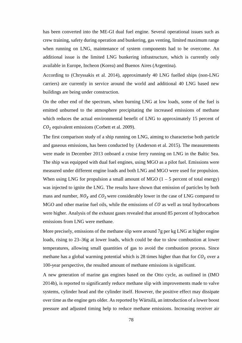
78
has been converted into the ME-GI dual fuel engine. Several operational issues such as
crew training, safety during operation and bunkering, gas venting, limited maximum range
when running on LNG, maintenance of system components had to be overcome. An
additional issue is the limited LNG bunkering infrastructure, which is currently only
available in Europe, Incheon (Korea) and Buenos Aires (Argentina).
According to (Chryssakis et al. 2014), approximately 40 LNG fuelled ships (non-LNG
carriers) are currently in service around the world and additional 40 LNG based new
buildings are being under construction.
On the other end of the spectrum, when burning LNG at low loads, some of the fuel is
emitted unburned to the atmosphere precipitating the increased emissions of methane
which reduces the actual environmental benefit of LNG to approximately 15 percent of
𝐶𝐶𝐶𝐶2 equivalent emissions (Corbett et al. 2009).
The first comparison study of a ship running on LNG, aiming to characterise both particle
and gaseous emissions, has been conducted by (Anderson et al. 2015). The measurements
were made in December 2013 onboard a cruise ferry running on LNG in the Baltic Sea.
The ship was equipped with dual fuel engines, using MGO as a pilot fuel. Emissions were
measured under different engine loads and both LNG and MGO were used for propulsion.
When using LNG for propulsion a small amount of MGO (1 – 5 percent of total energy)
was injected to ignite the LNG. The results have shown that emission of particles by both
mass and number, 𝑁𝑁𝐶𝐶𝑋𝑋 and 𝐶𝐶𝐶𝐶2 were considerably lower in the case of LNG compared to
MGO and other marine fuel oils, while the emissions of 𝐶𝐶𝐶𝐶 as well as total hydrocarbons
were higher. Analysis of the exhaust gases revealed that around 85 percent of hydrocarbon
emissions from LNG were methane.
More precisely, emissions of the methane slip were around 7g per kg LNG at higher engine
loads, rising to 23–36g at lower loads, which could be due to slow combustion at lower
temperatures, allowing small quantities of gas to avoid the combustion process. Since
methane has a global warming potential which is 28 times higher than that for 𝐶𝐶𝐶𝐶2 over a
100-year perspective, the resulted amount of methane emissions is significant.
A new generation of marine gas engines based on the Otto cycle, as outlined in (IMO
2014b), is reported to significantly reduce methane slip with improvements made to valve
systems, cylinder head and the cylinder itself. However, the positive effect may dissipate
over time as the engine gets older. As reported by Wärtsilä, an introduction of a lower boost
pressure and adjusted timing help to reduce methane emissions. Increasing receiver air
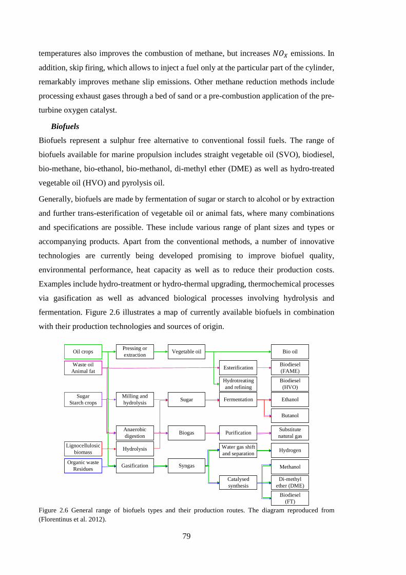
79
temperatures also improves the combustion of methane, but increases 𝑁𝑁𝐶𝐶𝑋𝑋 emissions. In
addition, skip firing, which allows to inject a fuel only at the particular part of the cylinder,
remarkably improves methane slip emissions. Other methane reduction methods include
processing exhaust gases through a bed of sand or a pre-combustion application of the pre-
turbine oxygen catalyst.
Biofuels
Biofuels represent a sulphur free alternative to conventional fossil fuels. The range of
biofuels available for marine propulsion includes straight vegetable oil (SVO), biodiesel,
bio-methane, bio-ethanol, bio-methanol, di-methyl ether (DME) as well as hydro-treated
vegetable oil (HVO) and pyrolysis oil.
Generally, biofuels are made by fermentation of sugar or starch to alcohol or by extraction
and further trans-esterification of vegetable oil or animal fats, where many combinations
and specifications are possible. These include various range of plant sizes and types or
accompanying products. Apart from the conventional methods, a number of innovative
technologies are currently being developed promising to improve biofuel quality,
environmental performance, heat capacity as well as to reduce their production costs.
Examples include hydro-treatment or hydro-thermal upgrading, thermochemical processes
via gasification as well as advanced biological processes involving hydrolysis and
fermentation. Figure 2.6 illustrates a map of currently available biofuels in combination
with their production technologies and sources of origin.
Oil crops
Waste oilAnimal fat
Lignocellulosicbiomass
SugarStarch crops
Organic wasteResidues
Pressing or extraction
Milling and hydrolysis
Anaerobic digestion
Hydrolysis
Gasification
Vegetable oil
Sugar
Biogas
Syngas
Esterification
Hydrotreating and refining
Fermentation
Purification
Water gas shift and separation
Catalysed synthesis
Bio oil
Biodiesel (FAME)
Biodiesel (HVO)
Ethanol
Butanol
Substitute natural gas
Hydrogen
Methanol
Di-methyl ether (DME)
Biodiesel(FT)
Figure 2.6 General range of biofuels types and their production routes. The diagram reproduced from (Florentinus et al. 2012).
80
Regardless of a lack of practical application in-service, there are a number of studies and
industry opinions supporting the idea that most of the biofuels are technically compatible
with marine engines as well as could be mixed with conventional fuels. For instance,
biodiesel FAME (Fatty Acid Methyl Ester) and vegetable oils, as stated in (Corbett et al.
2009), can readily be used in-service without extensive modifications of the existing
propulsion system although, in their present state, they require careful fuel management in
order to prevent the clogging of filters. In turn, biodiesel could potentially substitute
distillate fuels while vegetable oils may become an alternative to residual fuels, such as
soybean oil which has already been used by the Mols Linien (Ferry line) in Denmark, as
reported by (Mcgill et al. 2013). However, more investments are needed to the fuel supply
chain in order to introduce these fuels. In addition, since the biofuel’s sources and
production methods are varying greatly, the final products have different consistency and
heat capacity, which, in fact, is generally lower than energy capacity of most conventional
marine fuels meaning that more biofuel quantity is needed to meet the ship’s power
demand.
With some biofuels, there are potential issues associated with long-term storage stability,
acidity and corrosion, lack of water-shedding, filter plugging, wax formation suggesting
that selection and adaptation of any type of biofuel require careful evaluation.
Although, as long as properly managed, biodiesel FAME (a refined version of vegetable
oils or animal fat) does not cause complications to the engine itself, there are some specific
problems associated with its long-term storage, since it is not compatible with certain non-
metallic and metallic materials. Therefore, an internal coating of a storage tank, non-
metallic and some metallic fuel‐wetted compounds may need to be adapted to FAME.
However, as outlined in (Mcgill et al. 2013), the main issue associated with FAME is
sustainability since its production generally relies on palm oil which conflicts with the
preservation of natural rain forests, making it an impractical solution for a long-term
perspective.
Another example is di-methyl ether (DME) that has been known for the last 20 years as a
substitute for diesel in small engines. This does not guarantee its sustainability in case of
large applications since DME together with methanol is attributed to the biofuels with a
low flashpoint and require additional safety measures (Florentinus et al. 2012). However,
as outlined in (Chryssakis et al. 2014), the biomass‐to‐methanol/DME has been receiving

81
a lot of attention lately, as it is anticipated to become the most energy‐efficient option by
2050.
In addition, the conversion of a marine propulsion system to methanol is considered to be
cheaper than LNG due to the relative simplicity of the methanol storage system.
Furthermore, since methanol has similar combustion properties with methane, it can be
used in marine dual-fuel engines, as outlined by Wärtsilä and MAN. In fact, the CEAS
engine calculator by MAN has recently included biofuels namely methane, ethane and
methanol in addition to the conventional fuel options for preliminary estimation of their
Tier III engines performance.
Currently, biofuels are significantly more expensive than oil derived fuels. However,
biocrude, commonly referred as pyrolysis oil, is potentially a very cheap option since it can
be produced from any sort of biowaste or residue. Similarly to fossil crude, biocrude can
be further refined into lighter (biodiesel) products. Among the first, in 2013 Wärtsilä has
successfully tested several low speed engines to burn pyrolysis oil resulting in a combined
capacity of 680 MW.
Finally, since biofuels have an organic origin, they biodegrade rapidly, providing relative
safety to the marine environment in case of a spill when compared to conventional fossil
marine fuels. Nevertheless, as outlined in (Florentinus et al. 2012), there is a challenge to
secure a required production volume, since a production scale of 300 M Tonnes of Oil
Equivalent (TOE) biodiesel based on a current state of technology, requires more than 5
percent of the global agricultural land.
Renewable energy sources
In the past decade, the utilisation of renewable energy has been a spotlight of attention for
a range of applications. For the shipping industry, the primary focus lies on solar energy
and wind power. The latter one can be produced on-board by sails and kites or Flettner
rotors. Some early trials to utilise wind energy as part of the propulsion system have been
made with wing-sails, which represent essentially rigid panels on a rotating mast. These
include the Walker Wingsail, fitted to the 6,500 DWT Ashington in 1986. The trials
demonstrated negligibly small energy benefit. However, some current projects, including
UT Wind Challenger and EffShip, are aiming to enhance the wing-sail principle of design;
for example, by allowing sails to reef down on telescoping masts in the case of heavy
weather or in-port situations.
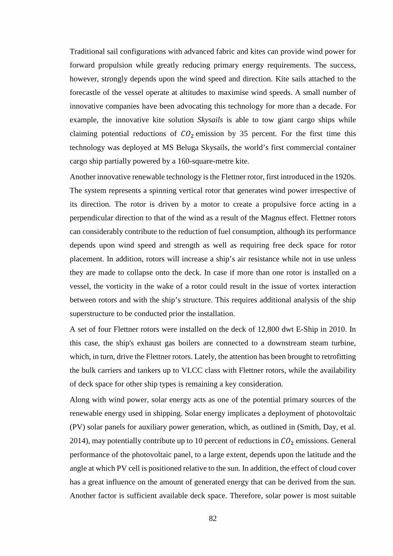
82
Traditional sail configurations with advanced fabric and kites can provide wind power for
forward propulsion while greatly reducing primary energy requirements. The success,
however, strongly depends upon the wind speed and direction. Kite sails attached to the
forecastle of the vessel operate at altitudes to maximise wind speeds. A small number of
innovative companies have been advocating this technology for more than a decade. For
example, the innovative kite solution Skysails is able to tow giant cargo ships while
claiming potential reductions of 𝐶𝐶𝐶𝐶2 emission by 35 percent. For the first time this
technology was deployed at MS Beluga Skysails, the world’s first commercial container
cargo ship partially powered by a 160-square-metre kite.
Another innovative renewable technology is the Flettner rotor, first introduced in the 1920s.
The system represents a spinning vertical rotor that generates wind power irrespective of
its direction. The rotor is driven by a motor to create a propulsive force acting in a
perpendicular direction to that of the wind as a result of the Magnus effect. Flettner rotors
can considerably contribute to the reduction of fuel consumption, although its performance
depends upon wind speed and strength as well as requiring free deck space for rotor
placement. In addition, rotors will increase a ship’s air resistance while not in use unless
they are made to collapse onto the deck. In case if more than one rotor is installed on a
vessel, the vorticity in the wake of a rotor could result in the issue of vortex interaction
between rotors and with the ship’s structure. This requires additional analysis of the ship
superstructure to be conducted prior the installation.
A set of four Flettner rotors were installed on the deck of 12,800 dwt E-Ship in 2010. In
this case, the ship's exhaust gas boilers are connected to a downstream steam turbine,
which, in turn, drive the Flettner rotors. Lately, the attention has been brought to retrofitting
the bulk carriers and tankers up to VLCC class with Flettner rotors, while the availability
of deck space for other ship types is remaining a key consideration.
Along with wind power, solar energy acts as one of the potential primary sources of the
renewable energy used in shipping. Solar energy implicates a deployment of photovoltaic
(PV) solar panels for auxiliary power generation, which, as outlined in (Smith, Day, et al.
2014), may potentially contribute up to 10 percent of reductions in 𝐶𝐶𝐶𝐶2 emissions. General
performance of the photovoltaic panel, to a large extent, depends upon the latitude and the
angle at which PV cell is positioned relative to the sun. In addition, the effect of cloud cover
has a great influence on the amount of generated energy that can be derived from the sun.
Another factor is sufficient available deck space. Therefore, solar power is most suitable
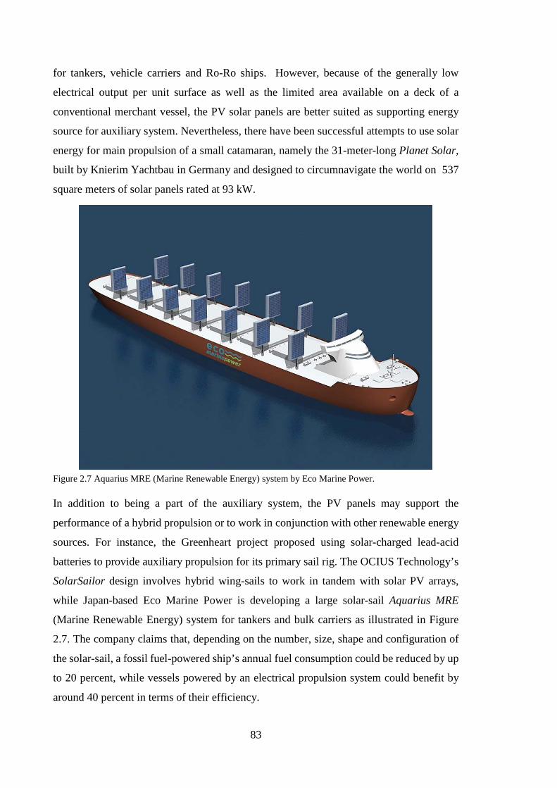
83
for tankers, vehicle carriers and Ro-Ro ships. However, because of the generally low
electrical output per unit surface as well as the limited area available on a deck of a
conventional merchant vessel, the PV solar panels are better suited as supporting energy
source for auxiliary system. Nevertheless, there have been successful attempts to use solar
energy for main propulsion of a small catamaran, namely the 31-meter-long Planet Solar,
built by Knierim Yachtbau in Germany and designed to circumnavigate the world on 537
square meters of solar panels rated at 93 kW.
Figure 2.7 Aquarius MRE (Marine Renewable Energy) system by Eco Marine Power.
In addition to being a part of the auxiliary system, the PV panels may support the
performance of a hybrid propulsion or to work in conjunction with other renewable energy
sources. For instance, the Greenheart project proposed using solar-charged lead-acid
batteries to provide auxiliary propulsion for its primary sail rig. The OCIUS Technology’s
SolarSailor design involves hybrid wing-sails to work in tandem with solar PV arrays,
while Japan-based Eco Marine Power is developing a large solar-sail Aquarius MRE
(Marine Renewable Energy) system for tankers and bulk carriers as illustrated in Figure
2.7. The company claims that, depending on the number, size, shape and configuration of
the solar-sail, a fossil fuel-powered ship’s annual fuel consumption could be reduced by up
to 20 percent, while vessels powered by an electrical propulsion system could benefit by
around 40 percent in terms of their efficiency.
84
Nuclear propulsion
Nuclear propulsion has many potential advantages associated with the emissions reduction.
Originally developed for the U.S. Navy in the 1950/60s, nuclear marine propulsion has
found its way to the civil application, in particular, icebreakers, where the first nuclear-
powered ship was the 20,000 DWT icebreaker, Lenin. In addition, there are four nuclear
powered civil cargo vessels that have been built, namely the first nuclear cargo/passenger
vessel Savannah by the United States (1962), German ore and passenger carrier Otto Hahn
(1970), Japanese nuclear-powered freighter Mutsu and the Russian container vessel
Sevmorput (1988). The most recent nuclear powered civil vessel is the Russian Arktika-
class icebreaker 50 Years of Victory (50 Let Pobedy) which was built in 2007.
Moreover, a new series LK-60 of Russian icebreakers is currently under development. This
includes the icebreaker Arctica, who’s keel was laid in November 2013 and is to be
delivered by the end of 2017. The LK-60 icebreaker is planned to be 173 m long and 34 m
wide while having a dual-draught with 33,530 tonnes displacement and designed to break
through 3 m thick ice at up to 2 knots. The LK-60 will be powered by two RITM-200
reactors with a thermal capacity of 175 MW each fuelled by low-enriched uranium fuel
(less than 20 percent). The propulsion power of this class of ships is 60MW to deliver at
the three propellers via twin turbine-generators and three motors. In addition, a more
powerful Russian LK-110 icebreaker of 110 MW net and 55,600 DWT is planned.
Generally, nuclear power plant generates high power from a very small volume of fuel by
fission of enriched uranium. Typically, a nuclear power plant requires refuelling only after
5-7 years, while new cores are designed to last up to 50 years. Therefore, since nuclear
fission does not have 𝐶𝐶𝐶𝐶2,𝑁𝑁𝐶𝐶𝑋𝑋 ,𝑆𝑆𝐶𝐶𝑋𝑋 and particulate matter emissions, there has been
growing interest attributed to the development of nuclear powered merchant vessels of a
new generation. The most common type of nuclear reactor is the uranium-fuelled
pressurised water reactor, where the energy is being released through the fission of 235U
coming from the following sources: the kinetic energy of the charged fission particles, the
energy of neutrinos as well as the gamma rays and the subsequent beta and gamma decay
(Carlton et al. 2011). For merchant applications, the level of enrichment of uranium is
limited by 20 percent by law.
To convert released chemical energy into the mechanical energy necessary for propulsion,
a geared steam turbine or turbo-generator are installed (Woud & Stapersma 2012). A geared
steam turbine plant is shown in Figure 2.8. While a nuclear power plant does not need air
85
compared to a boiler or a combustion engine, it does need an auxiliary backup system in
case of unexpected failure.
Typical nuclear power plant working principle is extensively described in (Carlton et al.
2011; Woud & Stapersma 2012). First, the released thermal energy from the fission process
heats up a primary water circuit, followed by a secondary water circuit consisting of the
water/steam system, similar to conventional steam plant while obtaining heat from the
primary circuit in a heat exchanger. In fact, the thermodynamic efficiency of this system is
lower compared to the conventional steam cycle.
Figure 2.8 Steam turbine plant powered by a nuclear reactor.
New types of nuclear reactor design have been recently proposed by a number of
manufacturers such as Mitsubishi, Toshiba and Hyperion Energy (Dedes et al. 2011),
namely smaller modular reactors which can be better described as a nuclear battery rather
than having a reactor propulsion layout. These reactors are fuelled with low enrichment
uranium while being compact (fitting into a twenty-foot container) and weighing up to two
tonnes per installed MWe.
In 2010 Lloyd's Register conducted a two-year research study in collaboration with US-
based Hyperion Power Generation (Gen4Energy), BMT Group, and Greek ship operator
Enterprises Shipping and Trading SA. The main purpose of this study was “to investigate
the practical maritime applications for small modular reactors". As part of this project

86
together with their other research studies, Lloyd's Register has updated its regulations for
nuclear ships concerning the integration of a nuclear reactor into ship system.
Arising from this research-collaboration project with Lloyd's Register, the (Hirdaris et al.
2014) report on commercial nuclear marine propulsion was published. The report
comprises past and recent work in the area of marine nuclear propulsion while describing
a preliminary concept design study for a 155,000 DWT tanker with a conventional hull
form but alternative arrangements for accommodating a 70 MWt nuclear propulsion plant.
The reactor was designed by Gen4Energy and has a potential to deliver up to 23.5 MW
shaft power at MCR. This is a small fast-neutron reactor using lead-bismuth eutectic
cooling and able to operate for ten full-power years before refuelling. As a result, the
concept has been considered feasible. However, the further maturity of nuclear technology
along with development and harmonisation of the regulatory framework is required.
Therefore, a widespread adoption of nuclear propulsion will face many constraints. One of
them being very high initial cost, estimated to be up to three times the cost of conventional
ships, (Dedes et al. 2011) as well as increased pricing for insurance and decommissioning.
In addition, there are potential harbour restrictions and uncertainty in legislation and safety
policy, which will need to particularly focus on the principle features of building, operating,
maintaining and decommissioning nuclear-powered vessels.
Hydrogen and fuel cells
Hydrogen, perhaps, is one of the most suitable yet innovative fuels theoretically applicable
for marine propulsions mainly due to its infinite source potential and clean burning
characteristics. Generally, hydrogen is the lightest gas offering the highest specific heat per
unit weight among other fuels. However, hydrogen can be difficult and expensive to
produce, transport and store. Hydrogen can be produced on-land by a nuclear power plant
and then transferred as fuel or, alternatively, on-board renewable energy sources can be
employed. Compressed hydrogen should be stored at high pressure (above 700 bars),
however, this requires six times more space compared to HFO while liquid hydrogen
should be transported at extremely low temperatures (-253 °C). This will significantly
impact the overall ship’s energy demand and require strongly insulated fuel tanks.
Fuel cells are the most commonly used devices to convert the chemical energy of hydrogen
into electrical energy with significantly higher efficiency, with noiseless operation and
without pollutant emissions compared with conventional combustion engines. However,
even though fuel cells do not have moving parts, they still require additional support
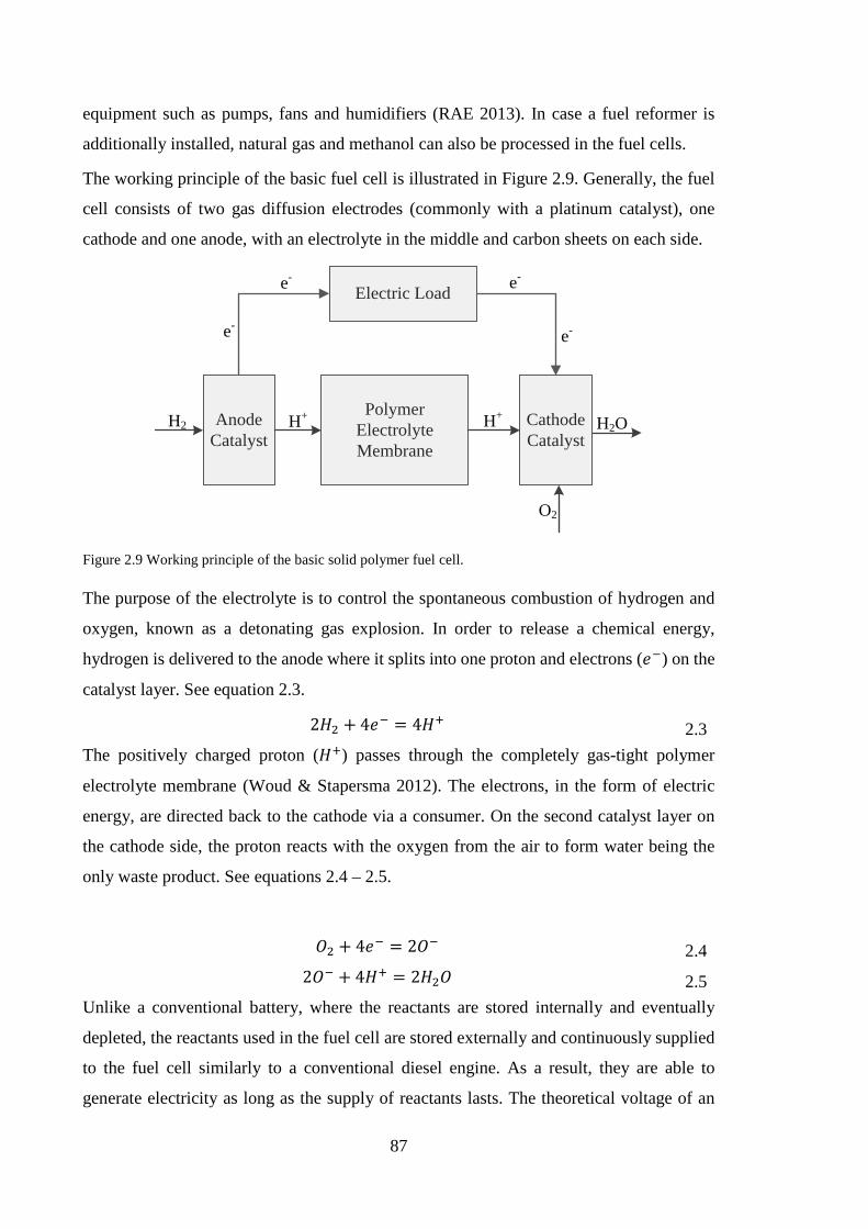
87
equipment such as pumps, fans and humidifiers (RAE 2013). In case a fuel reformer is
additionally installed, natural gas and methanol can also be processed in the fuel cells.
The working principle of the basic fuel cell is illustrated in Figure 2.9. Generally, the fuel
cell consists of two gas diffusion electrodes (commonly with a platinum catalyst), one
cathode and one anode, with an electrolyte in the middle and carbon sheets on each side.
Electric Load
Polymer Electrolyte Membrane
Cathode Catalyst
Anode Catalyst
H2 H+ H+ H2O
O2
e-
e- e-
e-
Figure 2.9 Working principle of the basic solid polymer fuel cell.
The purpose of the electrolyte is to control the spontaneous combustion of hydrogen and
oxygen, known as a detonating gas explosion. In order to release a chemical energy,
hydrogen is delivered to the anode where it splits into one proton and electrons (𝑒𝑒−) on the
catalyst layer. See equation 2.3.
2𝐻𝐻2 + 4𝑒𝑒− = 4𝐻𝐻+ 2.3 The positively charged proton (𝐻𝐻+) passes through the completely gas-tight polymer
electrolyte membrane (Woud & Stapersma 2012). The electrons, in the form of electric
energy, are directed back to the cathode via a consumer. On the second catalyst layer on
the cathode side, the proton reacts with the oxygen from the air to form water being the
only waste product. See equations 2.4 – 2.5.
𝐶𝐶2 + 4𝑒𝑒− = 2𝐶𝐶− 2.4 2𝐶𝐶− + 4𝐻𝐻+ = 2𝐻𝐻2𝐶𝐶 2.5
Unlike a conventional battery, where the reactants are stored internally and eventually
depleted, the reactants used in the fuel cell are stored externally and continuously supplied
to the fuel cell similarly to a conventional diesel engine. As a result, they are able to
generate electricity as long as the supply of reactants lasts. The theoretical voltage of an

88
𝐻𝐻2 𝐶𝐶2⁄ fuel cell is 1.48 V, which is referred to the upper heat value of hydrogen. At zero-
load conditions, slightly more than one volt per cell is available. The cooling units or
bipolar plates, in combination with carbon diffusion layers, distribute the reactants
uniformly across the area of the cell, conduct the electrons across the stack, remove the
heat from the electrodes and separate the media from each other (Siemens 2013).
At the present time, several fuel cells technologies are commercially available while some
are still under development. Fuel cells for low power applications based on hydrogen and
oxygen as reactants with an incorporated fuel reformer needed to transform hydrocarbon
fuels. These include an alkaline fuel cell (AFC) which is widely used in the space missions
by NASA, a phosphoric acid fuel cell (PAFC), which is available on the market but having
a relatively low efficiency, as well as a solid polymer fuel cell (SPFC).
Fuel cell technologies without a fuel reformer, which are able to use hydrocarbon directly,
include a direct methanol fuel cell (DMFC), molten carbonate fuel cell (MCFC), and solid
oxide fuel cell (SOFC) where the latest two are still under development.
When compared to a conventional marine diesel engine, a fuel cell technology provides
higher efficiency and lower fuel consumption while keeping exhaust emissions at bay.
However, the volume and weight of a fuel cell plant are generally greater than in the case
of conventional marine engine with the same power range. In addition, the current cost of
a fuel cell system is estimated to be higher than marine diesel engine while its maintenance
is predicted to be significantly less expensive (RAE 2013).
Several other characteristics of fuel cells could provide benefits for specific applications.
The fact that fuel cells are of modular design enables flexibility in the arrangement of plant
components and could lead to a more cost-effective layout of power and cargo spaces and
of basic ship structure. Therefore, since the fuel cells are highly efficient, silent and
sustainable, they can become a part of the future power production on ships. Nevertheless,
further research and development are necessary to overcome certain challenges associated
with the high investment costs, dimensions and weight of the fuel cell plant as well as a
particular attention should be given to storage of hydrogen on-board and safety aspects. As
such, fuel cells might become a niche powering option, particularly in combination with
hybrid battery systems (Chryssakis et al. 2014).
Batteries and hybrid propulsion
Recent developments in battery technologies and marine hybridisation hold significant
promise for more energy efficient shipping, since electric and hybrid ships with battery
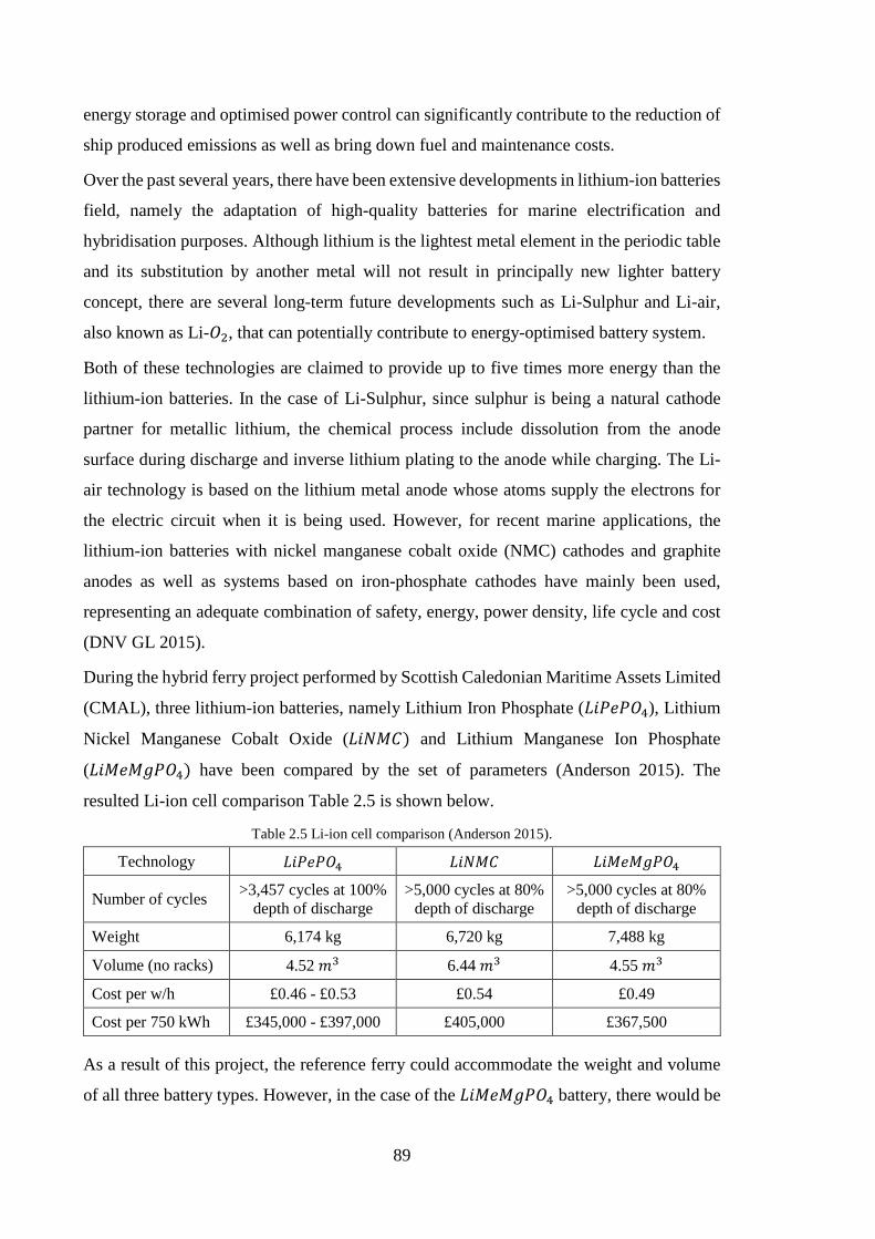
89
energy storage and optimised power control can significantly contribute to the reduction of
ship produced emissions as well as bring down fuel and maintenance costs.
Over the past several years, there have been extensive developments in lithium-ion batteries
field, namely the adaptation of high-quality batteries for marine electrification and
hybridisation purposes. Although lithium is the lightest metal element in the periodic table
and its substitution by another metal will not result in principally new lighter battery
concept, there are several long-term future developments such as Li-Sulphur and Li-air,
also known as Li-𝐶𝐶2, that can potentially contribute to energy-optimised battery system.
Both of these technologies are claimed to provide up to five times more energy than the
lithium-ion batteries. In the case of Li-Sulphur, since sulphur is being a natural cathode
partner for metallic lithium, the chemical process include dissolution from the anode
surface during discharge and inverse lithium plating to the anode while charging. The Li-
air technology is based on the lithium metal anode whose atoms supply the electrons for
the electric circuit when it is being used. However, for recent marine applications, the
lithium-ion batteries with nickel manganese cobalt oxide (NMC) cathodes and graphite
anodes as well as systems based on iron-phosphate cathodes have mainly been used,
representing an adequate combination of safety, energy, power density, life cycle and cost
(DNV GL 2015).
During the hybrid ferry project performed by Scottish Caledonian Maritime Assets Limited
(CMAL), three lithium-ion batteries, namely Lithium Iron Phosphate (𝐿𝐿𝑖𝑖𝑃𝑃𝑒𝑒𝑃𝑃𝐶𝐶4), Lithium
Nickel Manganese Cobalt Oxide (𝐿𝐿𝑖𝑖𝑁𝑁𝑁𝑁𝐶𝐶) and Lithium Manganese Ion Phosphate
(𝐿𝐿𝑖𝑖𝑁𝑁𝑒𝑒𝑁𝑁𝑔𝑔𝑃𝑃𝐶𝐶4) have been compared by the set of parameters (Anderson 2015). The
resulted Li-ion cell comparison Table 2.5 is shown below.
Table 2.5 Li-ion cell comparison (Anderson 2015).
Technology 𝐿𝐿𝑖𝑖𝑃𝑃𝑒𝑒𝑃𝑃𝐶𝐶4 𝐿𝐿𝑖𝑖𝑁𝑁𝑁𝑁𝐶𝐶 𝐿𝐿𝑖𝑖𝑁𝑁𝑒𝑒𝑁𝑁𝑔𝑔𝑃𝑃𝐶𝐶4
Number of cycles >3,457 cycles at 100% depth of discharge
>5,000 cycles at 80% depth of discharge
>5,000 cycles at 80% depth of discharge
Weight 6,174 kg 6,720 kg 7,488 kg
Volume (no racks) 4.52 𝑛𝑛3 6.44 𝑛𝑛3 4.55 𝑛𝑛3
Cost per w/h £0.46 - £0.53 £0.54 £0.49
Cost per 750 kWh £345,000 - £397,000 £405,000 £367,500
As a result of this project, the reference ferry could accommodate the weight and volume
of all three battery types. However, in the case of the 𝐿𝐿𝑖𝑖𝑁𝑁𝑒𝑒𝑁𝑁𝑔𝑔𝑃𝑃𝐶𝐶4 battery, there would be
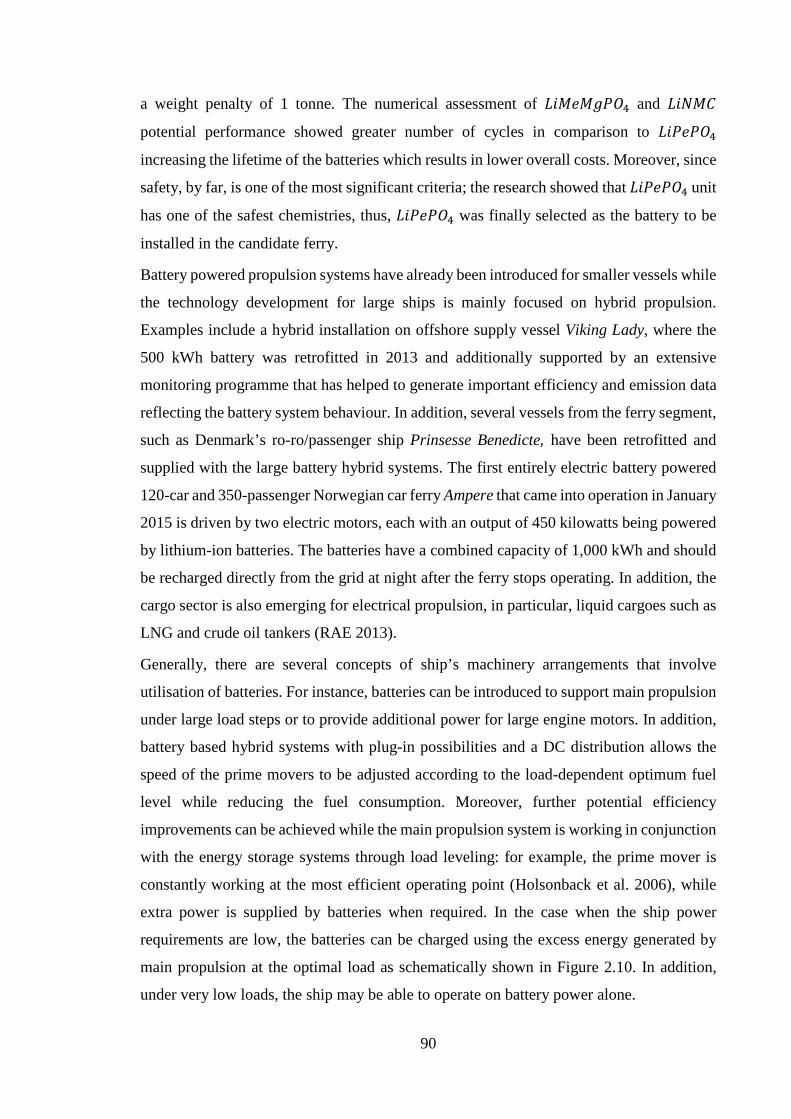
90
a weight penalty of 1 tonne. The numerical assessment of 𝐿𝐿𝑖𝑖𝑁𝑁𝑒𝑒𝑁𝑁𝑔𝑔𝑃𝑃𝐶𝐶4 and 𝐿𝐿𝑖𝑖𝑁𝑁𝑁𝑁𝐶𝐶
potential performance showed greater number of cycles in comparison to 𝐿𝐿𝑖𝑖𝑃𝑃𝑒𝑒𝑃𝑃𝐶𝐶4
increasing the lifetime of the batteries which results in lower overall costs. Moreover, since
safety, by far, is one of the most significant criteria; the research showed that 𝐿𝐿𝑖𝑖𝑃𝑃𝑒𝑒𝑃𝑃𝐶𝐶4 unit
has one of the safest chemistries, thus, 𝐿𝐿𝑖𝑖𝑃𝑃𝑒𝑒𝑃𝑃𝐶𝐶4 was finally selected as the battery to be
installed in the candidate ferry.
Battery powered propulsion systems have already been introduced for smaller vessels while
the technology development for large ships is mainly focused on hybrid propulsion.
Examples include a hybrid installation on offshore supply vessel Viking Lady, where the
500 kWh battery was retrofitted in 2013 and additionally supported by an extensive
monitoring programme that has helped to generate important efficiency and emission data
reflecting the battery system behaviour. In addition, several vessels from the ferry segment,
such as Denmark’s ro-ro/passenger ship Prinsesse Benedicte, have been retrofitted and
supplied with the large battery hybrid systems. The first entirely electric battery powered
120-car and 350-passenger Norwegian car ferry Ampere that came into operation in January
2015 is driven by two electric motors, each with an output of 450 kilowatts being powered
by lithium-ion batteries. The batteries have a combined capacity of 1,000 kWh and should
be recharged directly from the grid at night after the ferry stops operating. In addition, the
cargo sector is also emerging for electrical propulsion, in particular, liquid cargoes such as
LNG and crude oil tankers (RAE 2013).
Generally, there are several concepts of ship’s machinery arrangements that involve
utilisation of batteries. For instance, batteries can be introduced to support main propulsion
under large load steps or to provide additional power for large engine motors. In addition,
battery based hybrid systems with plug-in possibilities and a DC distribution allows the
speed of the prime movers to be adjusted according to the load-dependent optimum fuel
level while reducing the fuel consumption. Moreover, further potential efficiency
improvements can be achieved while the main propulsion system is working in conjunction
with the energy storage systems through load leveling: for example, the prime mover is
constantly working at the most efficient operating point (Holsonback et al. 2006), while
extra power is supplied by batteries when required. In the case when the ship power
requirements are low, the batteries can be charged using the excess energy generated by
main propulsion at the optimal load as schematically shown in Figure 2.10. In addition,
under very low loads, the ship may be able to operate on battery power alone.
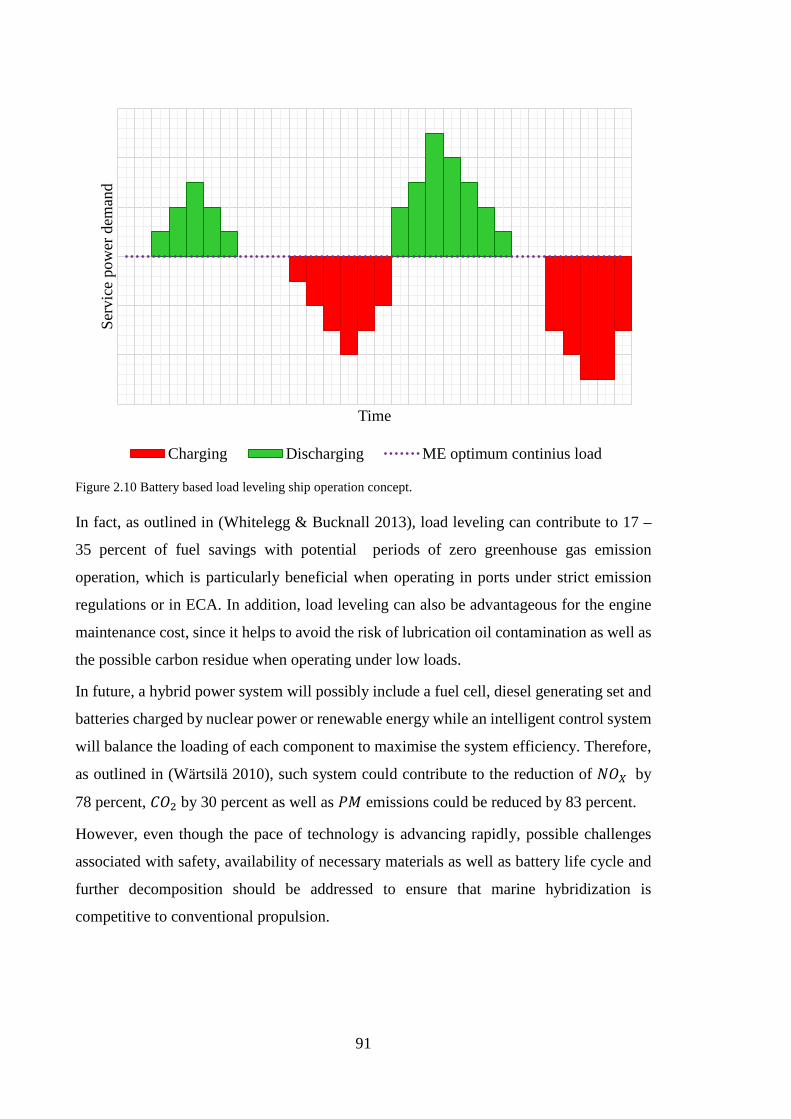
91
Figure 2.10 Battery based load leveling ship operation concept.
In fact, as outlined in (Whitelegg & Bucknall 2013), load leveling can contribute to 17 –
35 percent of fuel savings with potential periods of zero greenhouse gas emission
operation, which is particularly beneficial when operating in ports under strict emission
regulations or in ECA. In addition, load leveling can also be advantageous for the engine
maintenance cost, since it helps to avoid the risk of lubrication oil contamination as well as
the possible carbon residue when operating under low loads.
In future, a hybrid power system will possibly include a fuel cell, diesel generating set and
batteries charged by nuclear power or renewable energy while an intelligent control system
will balance the loading of each component to maximise the system efficiency. Therefore,
as outlined in (Wärtsilä 2010), such system could contribute to the reduction of 𝑁𝑁𝐶𝐶𝑋𝑋 by
78 percent, 𝐶𝐶𝐶𝐶2 by 30 percent as well as 𝑃𝑃𝑁𝑁 emissions could be reduced by 83 percent.
However, even though the pace of technology is advancing rapidly, possible challenges
associated with safety, availability of necessary materials as well as battery life cycle and
further decomposition should be addressed to ensure that marine hybridization is
competitive to conventional propulsion.
Serv
ice
pow
er d
eman
d
Time
Charging Discharging ME optimum continius load
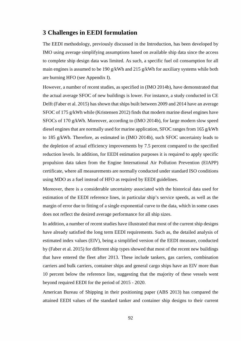
92
3 Challenges in EEDI formulation
The EEDI methodology, previously discussed in the Introduction, has been developed by
IMO using average simplifying assumptions based on available ship data since the access
to complete ship design data was limited. As such, a specific fuel oil consumption for all
main engines is assumed to be 190 g/kWh and 215 g/kWh for auxiliary systems while both
are burning HFO (see Appendix I).
However, a number of recent studies, as specified in (IMO 2014b), have demonstrated that
the actual average SFOC of new buildings is lower. For instance, a study conducted in CE
Delft (Faber et al. 2015) has shown that ships built between 2009 and 2014 have an average
SFOC of 175 g/kWh while (Kristensen 2012) finds that modern marine diesel engines have
SFOCs of 170 g/kWh. Moreover, according to (IMO 2014b), for large modern slow speed
diesel engines that are normally used for marine application, SFOC ranges from 165 g/kWh
to 185 g/kWh. Therefore, as estimated in (IMO 2014b), such SFOC uncertainty leads to
the depletion of actual efficiency improvements by 7.5 percent compared to the specified
reduction levels. In addition, for EEDI estimation purposes it is required to apply specific
propulsion data taken from the Engine International Air Pollution Prevention (EIAPP)
certificate, where all measurements are normally conducted under standard ISO conditions
using MDO as a fuel instead of HFO as required by EEDI guidelines.
Moreover, there is a considerable uncertainty associated with the historical data used for
estimation of the EEDI reference lines, in particular ship’s service speeds, as well as the
margin of error due to fitting of a single exponential curve to the data, which in some cases
does not reflect the desired average performance for all ship sizes.
In addition, a number of recent studies have illustrated that most of the current ship designs
have already satisfied the long term EEDI requirements. Such as, the detailed analysis of
estimated index values (EIV), being a simplified version of the EEDI measure, conducted
by (Faber et al. 2015) for different ship types showed that most of the recent new buildings
that have entered the fleet after 2013. These include tankers, gas carriers, combination
carriers and bulk carriers, container ships and general cargo ships have an EIV more than
10 percent below the reference line, suggesting that the majority of these vessels went
beyond required EEDI for the period of 2015 - 2020.
American Bureau of Shipping in their positioning paper (ABS 2013) has compared the
attained EEDI values of the standard tanker and container ship designs to their current

93
reference lines as well as the reference lines reduced by 10 percent. The considered ship
designs were based on the principal dimensions and service speeds typical for those built
in the last ten years. The corresponding propulsion power values were based on the
efficiency that is specific to the modern designs and the results have shown that all of the
standard tankers and containerships have satisfied the current reference line, while most of
them have met the EEDI requirements through 2020.
These facts introduce a question whether the EEDI measure will stimulate the efficiency
design improvements of vessels that have already satisfied its requirements. For instance,
Bazari and Longve in (IMO MEPC 63/INF.2 et al. 2011) have assumed that the level of
improvement in the average attained EEDI value will be larger than the level required by
EEDI reference lines for all ships except the most efficient ones while Anink and Krikke
in (Anink & Krikke 2011) have concluded that only the design of ships above the reference
line will be affected.
Finally, in some cases, as outlined in (ABS 2013), the EEDI measure does not reflect actual
efficiency benefits of some ship design features. For example, a comparison assessment of
the neopanamax and panamax container ship designs, has shown that even though the
neopanamax is more economically efficient than the panamax design, since the fuel oil
consumption per tonne-nm of cargo transported for the neopanamax containership was
approximately 14 percent less than the panamax containership of the same nominal TEU
capacity, the EEDI methodology rates the panamax design as more energy efficient. The
reason is that the hull of the panamax containership have a higher length/beam ratio making
it hydrodynamically more efficient. However, the wider beam on the neopanamax
containership enables a more stable hull form and, thus, significantly reduces the need for
ballast. As such, since EEDI uses DWT instead of TEU as a capacity measure, it could not
reflect the differences between a tonne of cargo and a tonne of ballast.
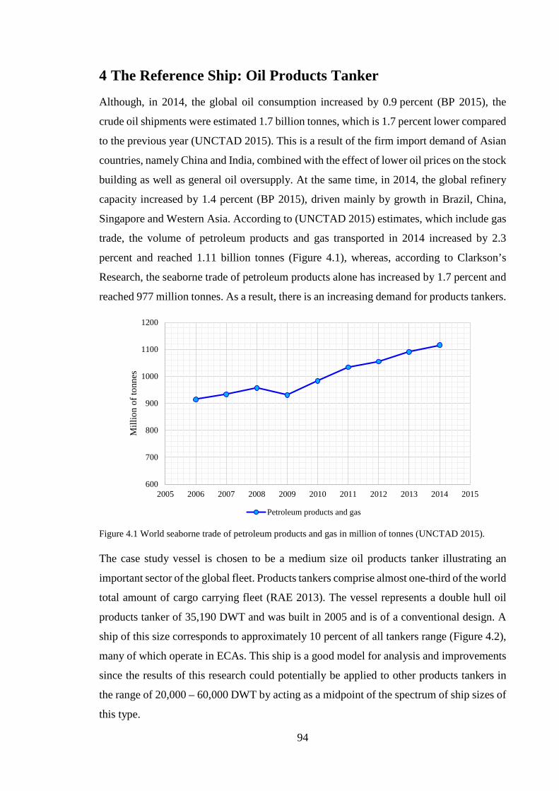
94
4 The Reference Ship: Oil Products Tanker
Although, in 2014, the global oil consumption increased by 0.9 percent (BP 2015), the
crude oil shipments were estimated 1.7 billion tonnes, which is 1.7 percent lower compared
to the previous year (UNCTAD 2015). This is a result of the firm import demand of Asian
countries, namely China and India, combined with the effect of lower oil prices on the stock
building as well as general oil oversupply. At the same time, in 2014, the global refinery
capacity increased by 1.4 percent (BP 2015), driven mainly by growth in Brazil, China,
Singapore and Western Asia. According to (UNCTAD 2015) estimates, which include gas
trade, the volume of petroleum products and gas transported in 2014 increased by 2.3
percent and reached 1.11 billion tonnes (Figure 4.1), whereas, according to Clarkson’s
Research, the seaborne trade of petroleum products alone has increased by 1.7 percent and
reached 977 million tonnes. As a result, there is an increasing demand for products tankers.
Figure 4.1 World seaborne trade of petroleum products and gas in million of tonnes (UNCTAD 2015).
The case study vessel is chosen to be a medium size oil products tanker illustrating an
important sector of the global fleet. Products tankers comprise almost one-third of the world
total amount of cargo carrying fleet (RAE 2013). The vessel represents a double hull oil
products tanker of 35,190 DWT and was built in 2005 and is of a conventional design. A
ship of this size corresponds to approximately 10 percent of all tankers range (Figure 4.2),
many of which operate in ECAs. This ship is a good model for analysis and improvements
since the results of this research could potentially be applied to other products tankers in
the range of 20,000 – 60,000 DWT by acting as a midpoint of the spectrum of ship sizes of
this type.
600
700
800
900
1000
1100
1200
2005 2006 2007 2008 2009 2010 2011 2012 2013 2014 2015
Mill
ion
of to
nnes
Petroleum products and gas
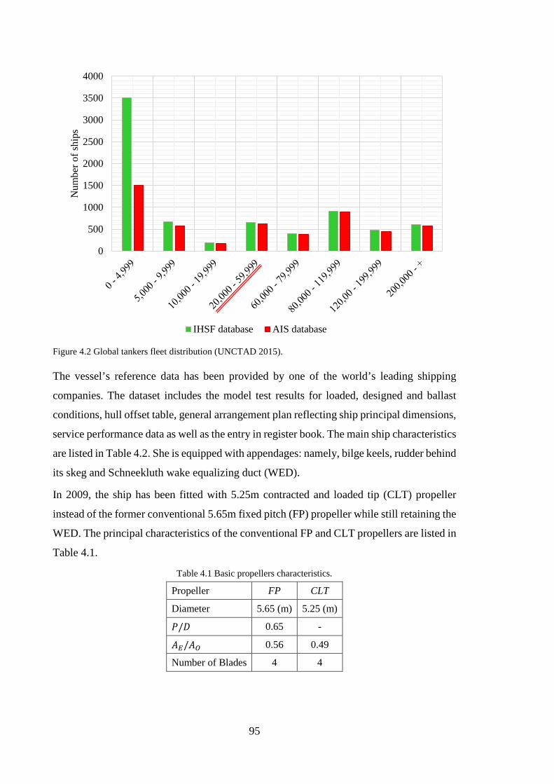
95
Figure 4.2 Global tankers fleet distribution (UNCTAD 2015).
The vessel’s reference data has been provided by one of the world’s leading shipping
companies. The dataset includes the model test results for loaded, designed and ballast
conditions, hull offset table, general arrangement plan reflecting ship principal dimensions,
service performance data as well as the entry in register book. The main ship characteristics
are listed in Table 4.2. She is equipped with appendages: namely, bilge keels, rudder behind
its skeg and Schneekluth wake equalizing duct (WED).
In 2009, the ship has been fitted with 5.25m contracted and loaded tip (CLT) propeller
instead of the former conventional 5.65m fixed pitch (FP) propeller while still retaining the
WED. The principal characteristics of the conventional FP and CLT propellers are listed in
Table 4.1.
Table 4.1 Basic propellers characteristics.
Propeller FP CLT
Diameter 5.65 (m) 5.25 (m)
𝑃𝑃/𝐷𝐷 0.65 -
𝐵𝐵𝐸𝐸/𝐵𝐵𝑂𝑂 0.56 0.49
Number of Blades 4 4
0
500
1000
1500
2000
2500
3000
3500
4000N
umbe
r of s
hips
IHSF database AIS database
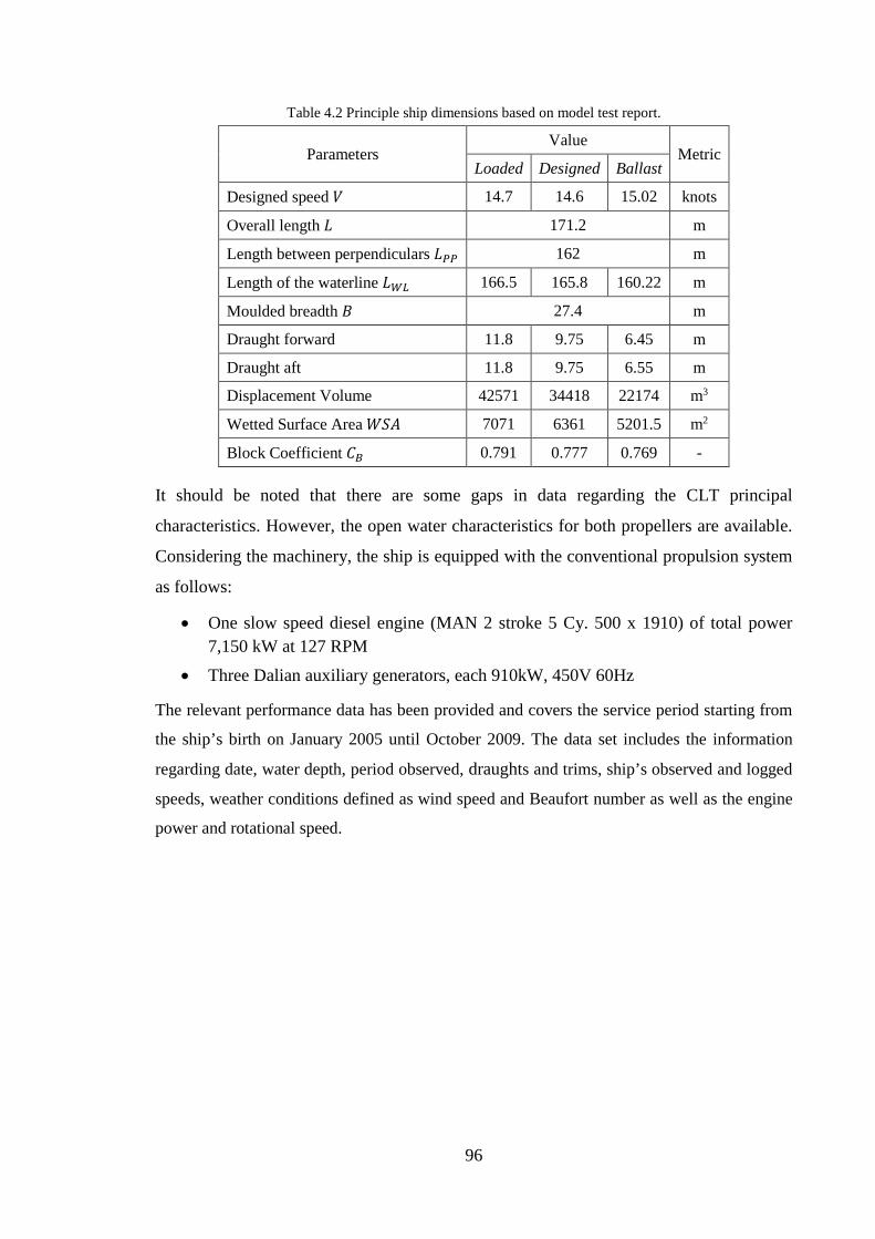
96
Table 4.2 Principle ship dimensions based on model test report.
Parameters Value
Metric Loaded Designed Ballast
Designed speed 𝑁𝑁 14.7 14.6 15.02 knots
Overall length 𝐿𝐿 171.2 m
Length between perpendiculars 𝐿𝐿𝑃𝑃𝑃𝑃 162 m
Length of the waterline 𝐿𝐿𝑊𝑊𝑊𝑊 166.5 165.8 160.22 m
Moulded breadth 𝐵𝐵 27.4 m
Draught forward 11.8 9.75 6.45 m
Draught aft 11.8 9.75 6.55 m
Displacement Volume 42571 34418 22174 m3
Wetted Surface Area 𝑊𝑊𝑆𝑆𝐵𝐵 7071 6361 5201.5 m2
Block Coefficient 𝐶𝐶𝐵𝐵 0.791 0.777 0.769 -
It should be noted that there are some gaps in data regarding the CLT principal
characteristics. However, the open water characteristics for both propellers are available.
Considering the machinery, the ship is equipped with the conventional propulsion system
as follows:
• One slow speed diesel engine (MAN 2 stroke 5 Cy. 500 x 1910) of total power 7,150 kW at 127 RPM
• Three Dalian auxiliary generators, each 910kW, 450V 60Hz
The relevant performance data has been provided and covers the service period starting from
the ship’s birth on January 2005 until October 2009. The data set includes the information
regarding date, water depth, period observed, draughts and trims, ship’s observed and logged
speeds, weather conditions defined as wind speed and Beaufort number as well as the engine
power and rotational speed.

97
PhD Research Structure Based on the assessment of current energy efficiency-enhancing technologies and methods
along with the available ship, propellers and service data, the following research structure
includes a purpose developed computer basis ship simulation model as a base for the
number of case studies. The short summary of each case study is briefly described below
while a detailed explanation along with its relevance based on the literature review,
calculation procedure, results and conclusions are presented in each of the following
chapters.
As such, Chapter 5 is dedicated to a detailed description of the computer based ship
simulation model with specified range of methods and algorithms used. The ship simulation
model, referred to Ship Performance Simulation model (SPS), is then verified and
correlated with the available data to ensure its correct performance. In addition, this chapter
describes the energy efficiency measures developed in this study to compare the ship
energy efficiency behaviour under different conditions, namely the Energy Efficiency
Indicators (EEI) comprising propulsion efficiency, fuel consumption, exhaust emissions
flow rate as well as EEDI index.
A time domain voyage simulation model is described in Chapter 6. This model predicts the
power increase due to changing weather based on the ship’s service data in combination
with the trial allowances approach. The voyage simulation acts as a base for the estimation
of potential fuel and emissions reductions due to the introduction of various energy saving
technologies and methods in the following chapters.
Chapter 7 focuses on the high-efficiency propellers analysis, namely the effect of wake
equalising duct on ship efficiency as well as the comparison analysis of conventional fixed
pitch, CLT and ducted propellers and their effect on ship propulsion behaviour under ballast
and loaded conditions.
Propeller optimisation strategies are discussed in Chapter 8. The case study is based on a
conventional fixed pitch propeller and include the analysis of the effect of reduced blade
area ratio (BAR) as well as artificially increased propeller diameters on propulsion
efficiency with reference to propeller cavitation margins.
Chapter 9 explores the low RPM/increased diameter propeller design concept by
comparing two conventional fixed pitch propellers with the maximised diameter. The first
represents a maximum diameter that could be fitted into the current ship arrangement while
second illustrates the maximum possible diameter with a relocated shaft. The study answers

98
a question of whether the maximising of the propeller diameter to its limit while changing
stern arrangements would bring a significant difference to the fuel consumption and EEDI
value.
Chapter 10 is focused on the effect of trim on ship resistance and, therefore, fuel
consumption and exhaust emissions flow. This case study is centred on a partly loaded
condition with changing forward trim. Along with ship resistance, the analysis has also
covered propulsion characteristics and propeller efficiency.
Chapter 11 is dedicated to innovative, for the shipping industry, hybrid propulsion concepts
also referred as load levelling. This allows to continuously operate at the most efficient
load while charging and discharging batteries. This case study is looking at the load leveling
operation under changing weather conditions in order to estimate potential long-term
efficiency benefits as well as the effect on the level of atmospheric emissions.
Finally, Chapter 12 is focused on the EEDI formulation philosophy, where EEDI values
have been estimated in accordance with ships’ performance data and further analysed under
changing weather conditions (Beaufort number). This has helped to uncover some potential
uncertainties associated with the effect of real sea state on EEDI index and ship’s energy
efficiency level while providing recommendations and strategies on how they might be
improved.
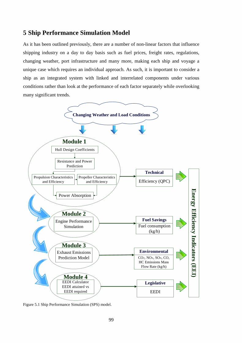
99
5 Ship Performance Simulation Model
As it has been outlined previously, there are a number of non-linear factors that influence
shipping industry on a day to day basis such as fuel prices, freight rates, regulations,
changing weather, port infrastructure and many more, making each ship and voyage a
unique case which requires an individual approach. As such, it is important to consider a
ship as an integrated system with linked and interrelated components under various
conditions rather than look at the performance of each factor separately while overlooking
many significant trends.
Hull Design Coefficients
Resistance and Power Prediction
Propulsion Characteristics and Efficiency
Power Absorption
Propeller Characteristics and Efficiency
Module 1
Engine Performance Simulation
Module 2
Exhaust Emissions Prediction Model
Module 3
EEDI CalculatorEEDI attained vs EEDI required
Module 4
Efficiency (QPC)
Fuel consumption (kg/h)
CO2, NOX, SOX, CO, HC Emissions Mass
Flow Rate (kg/h)
EEDI
Technical
Fuel Savings
Environmental
Legislative
Energy Efficiency Indicators (EEI)
Changing Weather and Load Conditions
Figure 5.1 Ship Performance Simulation (SPS) model.

100
Therefore, in order to undertake a number of case studies regarding the implementation of
various methods and strategies designed to enhance ship energy efficiency, a computer-
based integrated ship simulation model, namely Ship Performance Simulation (SPS)
model, has been developed in a connected Matlab and Excel environment operating in both
steady state and time domain modes. The model consists of four fundamental modules as
schematically shown in Figure 5.1.
The modules are ship resistance and propulsion simulation model, engine performance
model, exhaust emissions prediction model and the EEDI calculator. Each module has a
number of outputs, used as inputs into the subsequent modules. However, in order to
compare the ship’s performance in different case studies, each module has an output that is
considered as an energy efficiency indicator (EEI) reflecting one of four outlined forces.
The first module has an overall propulsion efficiency (QPC) as an indicator of technological
performance, the second module has a fuel consumption output to evaluate the cost-
effectiveness of a proposed technology or method. The third module demonstrates an
exhaust emissions footprint as an environmental indicator while the fourth module
estimates the EEDI index acting as an indicator of the legal feasibility in coming years.
Moreover, the system would not be complete without the ship performance analysis under
different loads such as ballast/loaded and changing weather. Therefore, ship performance
results are also analysed using the time domain simulation taking into account the ship’s
speed and load behaviour as well as sea state distribution in accordance with the provided
service data, where the effect of weather is evaluated using the Beaufort wind force scale
for fully developed seas.
It is important to emphasise that approaches and methods used in some modules may vary
in different case studies while in this chapter the fundamental principles of each module as
well as a time-domain model have been described and validated in accordance with the
provided data.
Module 1: Resistance and Propulsion Based on William Froude’s similarity law stating that the wave-making resistance
coefficients of two geometrically similar models are the same when towing with the same
speed to length ratio, in combination with additional dimensionless analysis, the ship’s total
resistance coefficient 𝐶𝐶𝑇𝑇 can be described as follows:
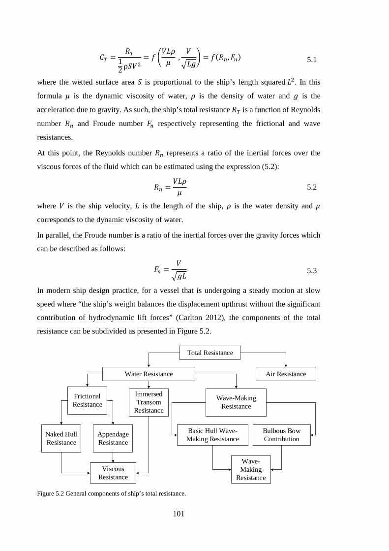
101
𝐶𝐶𝑇𝑇 =𝐵𝐵𝑇𝑇
12 ρ𝑆𝑆𝑁𝑁
2= 𝑓𝑓
𝑁𝑁𝐿𝐿𝑉𝑉𝜇𝜇
,𝑁𝑁𝐿𝐿𝑔𝑔
= 𝑓𝑓(𝐵𝐵𝐴𝐴,𝑆𝑆𝐴𝐴) 5.1
where the wetted surface area 𝑆𝑆 is proportional to the ship’s length squared 𝐿𝐿2. In this
formula 𝜇𝜇 is the dynamic viscosity of water, 𝑉𝑉 is the density of water and 𝑔𝑔 is the
acceleration due to gravity. As such, the ship’s total resistance 𝐵𝐵𝑇𝑇 is a function of Reynolds
number 𝐵𝐵𝐴𝐴 and Froude number 𝑆𝑆𝐴𝐴 respectively representing the frictional and wave
resistances.
At this point, the Reynolds number 𝐵𝐵𝐴𝐴 represents a ratio of the inertial forces over the
viscous forces of the fluid which can be estimated using the expression (5.2):
𝐵𝐵𝐴𝐴 =𝑁𝑁𝐿𝐿𝑉𝑉𝜇𝜇
5.2
where 𝑁𝑁 is the ship velocity, 𝐿𝐿 is the length of the ship, 𝑉𝑉 is the water density and 𝜇𝜇
corresponds to the dynamic viscosity of water.
In parallel, the Froude number is a ratio of the inertial forces over the gravity forces which
can be described as follows:
𝑆𝑆𝐴𝐴 =𝑁𝑁𝑔𝑔𝐿𝐿
5.3
In modern ship design practice, for a vessel that is undergoing a steady motion at slow
speed where “the ship’s weight balances the displacement upthrust without the significant
contribution of hydrodynamic lift forces” (Carlton 2012), the components of the total
resistance can be subdivided as presented in Figure 5.2.
Total Resistance
Water Resistance Air Resistance
Frictional Resistance
Immersed Transom
Resistance
Wave-Making Resistance
Appendage Resistance
Naked Hull Resistance
Basic Hull Wave-Making Resistance
Bulbous Bow Contribution
Wave-Making
Resistance Viscous
Resistance
Figure 5.2 General components of ship’s total resistance.
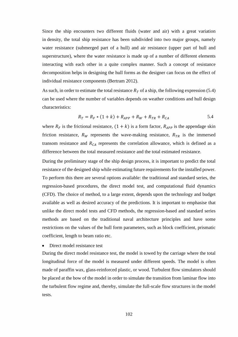
102
Since the ship encounters two different fluids (water and air) with a great variation
in density, the total ship resistance has been subdivided into two major groups, namely
water resistance (submerged part of a hull) and air resistance (upper part of hull and
superstructure), where the water resistance is made up of a number of different elements
interacting with each other in a quite complex manner. Such a concept of resistance
decomposition helps in designing the hull forms as the designer can focus on the effect of
individual resistance components (Bertram 2012).
As such, in order to estimate the total resistance 𝐵𝐵𝑇𝑇 of a ship, the following expression (5.4)
can be used where the number of variables depends on weather conditions and hull design
characteristics:
𝐵𝐵𝑇𝑇 = 𝐵𝐵𝐹𝐹 ∗ (1 + 𝑘𝑘) + 𝐵𝐵𝐴𝐴𝑃𝑃𝑃𝑃 + 𝐵𝐵𝑊𝑊 + 𝐵𝐵𝑇𝑇𝑅𝑅 + 𝐵𝐵𝐶𝐶𝐴𝐴 5.4
where 𝐵𝐵𝐹𝐹 is the frictional resistance, (1 + 𝑘𝑘) is a form factor, 𝐵𝐵𝐴𝐴𝑃𝑃𝑃𝑃 is the appendage skin
friction resistance, 𝐵𝐵𝑊𝑊 represents the wave-making resistance, 𝐵𝐵𝑇𝑇𝑅𝑅 is the immersed
transom resistance and 𝐵𝐵𝐶𝐶𝐴𝐴 represents the correlation allowance, which is defined as a
difference between the total measured resistance and the total estimated resistance.
During the preliminary stage of the ship design process, it is important to predict the total
resistance of the designed ship while estimating future requirements for the installed power.
To perform this there are several options available: the traditional and standard series, the
regression-based procedures, the direct model test, and computational fluid dynamics
(CFD). The choice of method, to a large extent, depends upon the technology and budget
available as well as desired accuracy of the predictions. It is important to emphasise that
unlike the direct model tests and CFD methods, the regression-based and standard series
methods are based on the traditional naval architecture principles and have some
restrictions on the values of the hull form parameters, such as block coefficient, prismatic
coefficient, length to beam ratio etc.
• Direct model resistance test During the direct model resistance test, the model is towed by the carriage where the total
longitudinal force of the model is measured under different speeds. The model is often
made of paraffin wax, glass-reinforced plastic, or wood. Turbulent flow simulators should
be placed at the bow of the model in order to simulate the transition from laminar flow into
the turbulent flow regime and, thereby, simulate the full-scale flow structures in the model
tests.
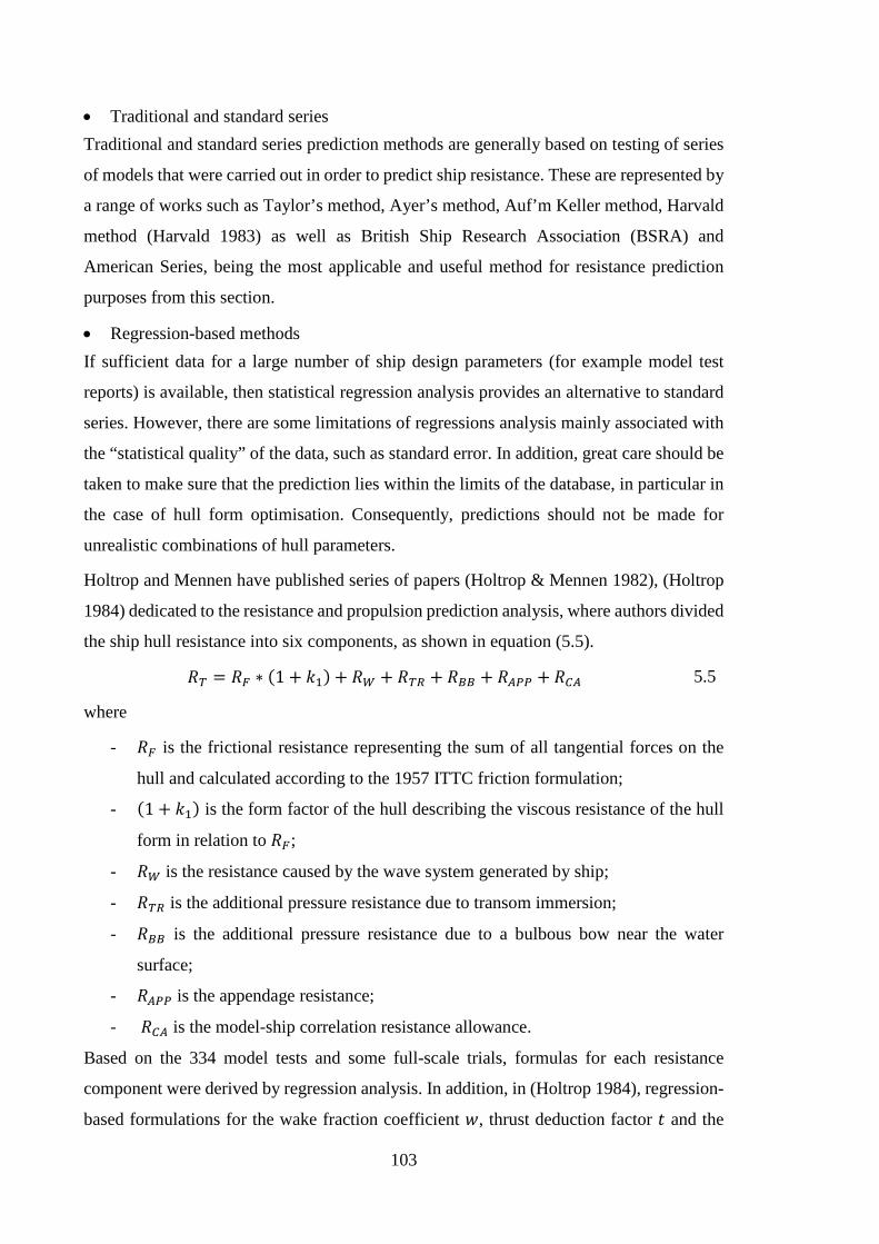
103
• Traditional and standard series Traditional and standard series prediction methods are generally based on testing of series
of models that were carried out in order to predict ship resistance. These are represented by
a range of works such as Taylor’s method, Ayer’s method, Auf’m Keller method, Harvald
method (Harvald 1983) as well as British Ship Research Association (BSRA) and
American Series, being the most applicable and useful method for resistance prediction
purposes from this section.
• Regression-based methods If sufficient data for a large number of ship design parameters (for example model test
reports) is available, then statistical regression analysis provides an alternative to standard
series. However, there are some limitations of regressions analysis mainly associated with
the “statistical quality” of the data, such as standard error. In addition, great care should be
taken to make sure that the prediction lies within the limits of the database, in particular in
the case of hull form optimisation. Consequently, predictions should not be made for
unrealistic combinations of hull parameters.
Holtrop and Mennen have published series of papers (Holtrop & Mennen 1982), (Holtrop
1984) dedicated to the resistance and propulsion prediction analysis, where authors divided
the ship hull resistance into six components, as shown in equation (5.5).
𝐵𝐵𝑇𝑇 = 𝐵𝐵𝐹𝐹 ∗ (1 + 𝑘𝑘1) + 𝐵𝐵𝑊𝑊 + 𝐵𝐵𝑇𝑇𝑅𝑅 + 𝐵𝐵𝐵𝐵𝐵𝐵 + 𝐵𝐵𝐴𝐴𝑃𝑃𝑃𝑃 + 𝐵𝐵𝐶𝐶𝐴𝐴 5.5
where
- 𝐵𝐵𝐹𝐹 is the frictional resistance representing the sum of all tangential forces on the
hull and calculated according to the 1957 ITTC friction formulation;
- (1 + 𝑘𝑘1) is the form factor of the hull describing the viscous resistance of the hull
form in relation to 𝐵𝐵𝐹𝐹;
- 𝐵𝐵𝑊𝑊 is the resistance caused by the wave system generated by ship;
- 𝐵𝐵𝑇𝑇𝑅𝑅 is the additional pressure resistance due to transom immersion;
- 𝐵𝐵𝐵𝐵𝐵𝐵 is the additional pressure resistance due to a bulbous bow near the water
surface;
- 𝐵𝐵𝐴𝐴𝑃𝑃𝑃𝑃 is the appendage resistance;
- 𝐵𝐵𝐶𝐶𝐴𝐴 is the model-ship correlation resistance allowance.
Based on the 334 model tests and some full-scale trials, formulas for each resistance
component were derived by regression analysis. In addition, in (Holtrop 1984), regression-
based formulations for the wake fraction coefficient 𝑤𝑤, thrust deduction factor 𝐶𝐶 and the

104
propeller relative-rotative efficiency 𝜂𝜂𝑅𝑅 are presented. The formulation and implementation
of these factors are discussed later in this section. However, this approach is only suitable
for the standard ship designs as the more complex or non-conventional ship forms may
affect its accuracy.
Another regression-based approach has been carried out by Hollenbach (Hollenbach 1998)
based on the results of resistance tests on 433 models at the Vienna Ship Model Basin from
1980 to 1995. The models were both, of single-screw and twin-screw ships. In this method,
the data has been analysed and presented in two ways depending on the application and
available data. A ‘mean’ value of resistance is calculated when normal constraints on the
hull form are available for design purposes and a ‘minimum’ resistance which might be
achieved for hull parameters established after extensive optimisation of the ship lines if
ship’s design is not subject to restrictions.
In addition to length between perpendiculars 𝐿𝐿𝑃𝑃𝑃𝑃 and the waterline length 𝐿𝐿𝑊𝑊𝑊𝑊, Hollenbach
introduced a new term, a length over surface 𝐿𝐿𝑂𝑂𝑆𝑆, which in case of design draught means
length between the aft end of design waterline and the most forward point of ship below
design waterline, while for ballast draught 𝐿𝐿𝑂𝑂𝑆𝑆 represents length between aft end and
forward end of ballast waterline, where rudder is not taken into account.
• Computational fluid dynamics (CFD) CFD allows the investigator to predict ship’s resistance curve and further mathematical
modelling of three-dimensional fluid flow using one of the following methods: the finite
element method of analysis (FEM), boundary element methods (BEM), finite difference
method (FDM) or finite volume methods (FVM), specified in (Bertram 2012; Carlton
2012). According to (Bertram 2012) FVM, FDM and FEM are referred to “field methods”,
as they use discretization of the whole fluid field. Alternatively, the boundary element
method can be applied to discretise the boundaries. However, in these computationally
based analyses turbulence modelling has been problematic. Reasonable estimates of the
frictional resistance have been made for fine form ships using 𝑘𝑘 − Ω and 𝑘𝑘 − Ω shear stress
transport (SST) models, while the more computationally intensive Reynolds stress models
have improved the accuracy of the prediction for the finer hull forms.
CFD requires a high-performance computer as there is an ample quantity of equations to
be solved. The water flow dynamic simulation is very complex, especially flow around a
stern and, in many cases, it is difficult to analyse it using the computer modelling.
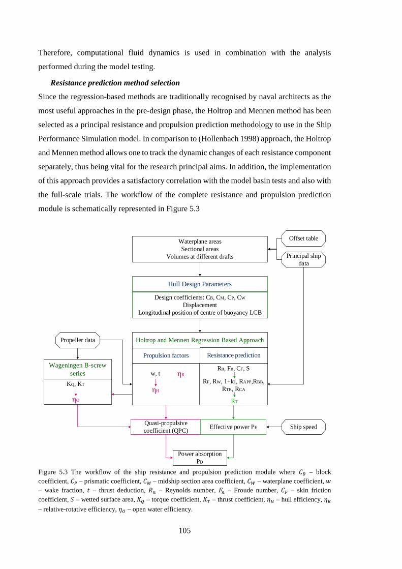
105
Therefore, computational fluid dynamics is used in combination with the analysis
performed during the model testing.
Resistance prediction method selection
Since the regression-based methods are traditionally recognised by naval architects as the
most useful approaches in the pre-design phase, the Holtrop and Mennen method has been
selected as a principal resistance and propulsion prediction methodology to use in the Ship
Performance Simulation model. In comparison to (Hollenbach 1998) approach, the Holtrop
and Mennen method allows one to track the dynamic changes of each resistance component
separately, thus being vital for the research principal aims. In addition, the implementation
of this approach provides a satisfactory correlation with the model basin tests and also with
the full-scale trials. The workflow of the complete resistance and propulsion prediction
module is schematically represented in Figure 5.3
Offset table
Principal ship data
Waterplane areasSectional areas
Volumes at different drafts
Design coefficients: CB, CM, CP, CW
DisplacementLongitudinal position of centre of buoyancy LCB
Hull Design Parameters
Propeller data
Wageningen B-screw series
Power absorption PD
Holtrop and Mennen Regression Based Approach
Resistance predictionPropulsion factors
Quasi-propulsive coefficient (QPC) Effective power PE Ship speed
w, t ηR
ηH KQ, KT
ηO
Rn, Fn, CF, S
RF, RW, 1+k1, RAPP,RBB, RTR, RCA
RT
Figure 5.3 The workflow of the ship resistance and propulsion prediction module where 𝐶𝐶𝐵𝐵 – block coefficient, 𝐶𝐶𝑃𝑃 – prismatic coefficient, 𝐶𝐶𝑀𝑀 – midship section area coefficient, 𝐶𝐶𝑊𝑊 – waterplane coefficient, 𝑤𝑤 – wake fraction, 𝐶𝐶 – thrust deduction, 𝐵𝐵𝐴𝐴 – Reynolds number, 𝑆𝑆𝐴𝐴 – Froude number, 𝐶𝐶𝐹𝐹 – skin friction coefficient, 𝑆𝑆 – wetted surface area, 𝐾𝐾𝑄𝑄 – torque coefficient, 𝐾𝐾𝑇𝑇 – thrust coefficient, 𝜂𝜂𝐻𝐻 – hull efficiency, 𝜂𝜂𝑅𝑅 – relative-rotative efficiency, 𝜂𝜂𝑂𝑂 – open water efficiency.
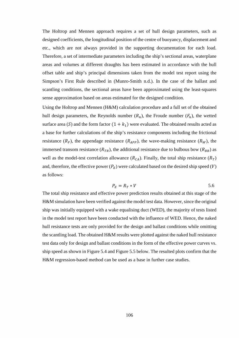
106
The Holtrop and Mennen approach requires a set of hull design parameters, such as
designed coefficients, the longitudinal position of the centre of buoyancy, displacement and
etc., which are not always provided in the supporting documentation for each load.
Therefore, a set of intermediate parameters including the ship’s sectional areas, waterplane
areas and volumes at different draughts has been estimated in accordance with the hull
offset table and ship’s principal dimensions taken from the model test report using the
Simpson’s First Rule described in (Munro-Smith n.d.). In the case of the ballast and
scantling conditions, the sectional areas have been approximated using the least-squares
sense approximation based on areas estimated for the designed condition.
Using the Holtrop and Mennen (H&M) calculation procedure and a full set of the obtained
hull design parameters, the Reynolds number (𝐵𝐵𝐴𝐴), the Froude number (𝑆𝑆𝐴𝐴), the wetted
surface area (𝑆𝑆) and the form factor (1 + 𝑘𝑘1) were evaluated. The obtained results acted as
a base for further calculations of the ship’s resistance components including the frictional
resistance (𝐵𝐵𝐹𝐹), the appendage resistance (𝐵𝐵𝐴𝐴𝑃𝑃𝑃𝑃), the wave-making resistance (𝐵𝐵𝑊𝑊), the
immersed transom resistance (𝐵𝐵𝑇𝑇𝑅𝑅), the additional resistance due to bulbous bow (𝐵𝐵𝐵𝐵𝐵𝐵) as
well as the model-test correlation allowance (𝐵𝐵𝐶𝐶𝐴𝐴). Finally, the total ship resistance (𝐵𝐵𝑇𝑇)
and, therefore, the effective power (𝑃𝑃𝐸𝐸) were calculated based on the desired ship speed (𝑁𝑁)
as follows:
𝑃𝑃𝐸𝐸 = 𝐵𝐵𝑇𝑇 ∗ 𝑁𝑁 5.6 The total ship resistance and effective power prediction results obtained at this stage of the
H&M simulation have been verified against the model test data. However, since the original
ship was initially equipped with a wake equalising duct (WED), the majority of tests listed
in the model test report have been conducted with the influence of WED. Hence, the naked
hull resistance tests are only provided for the design and ballast conditions while omitting
the scantling load. The obtained H&M results were plotted against the naked hull resistance
test data only for design and ballast conditions in the form of the effective power curves vs.
ship speed as shown in Figure 5.4 and Figure 5.5 below. The resulted plots confirm that the
H&M regression-based method can be used as a base in further case studies.
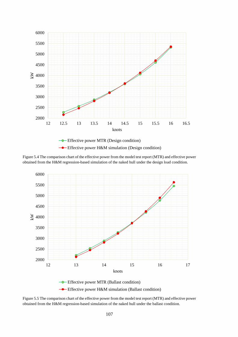
107
Figure 5.4 The comparison chart of the effective power from the model test report (MTR) and effective power obtained from the H&M regression-based simulation of the naked hull under the design load condition.
Figure 5.5 The comparison chart of the effective power from the model test report (MTR) and effective power obtained from the H&M regression-based simulation of the naked hull under the ballast condition.
2000
2500
3000
3500
4000
4500
5000
5500
6000
12 12.5 13 13.5 14 14.5 15 15.5 16 16.5
kW
knots
Effective power MTR (Design condition)Effective power H&M simulation (Design condition)
2000
2500
3000
3500
4000
4500
5000
5500
6000
12 13 14 15 16 17
kW
knots
Effective power MTR (Ballast condition)Effective power H&M simulation (Ballast condition)
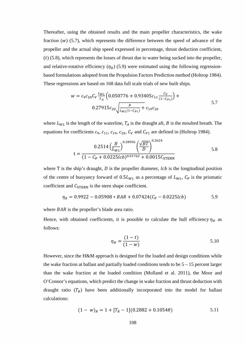
108
Thereafter, using the obtained results and the main propeller characteristics, the wake
fraction (𝑤𝑤) (5.7), which represents the difference between the speed of advance of the
propeller and the actual ship speed expressed in percentage, thrust deduction coefficient,
(𝐶𝐶) (5.8), which represents the losses of thrust due to water being sucked into the propeller,
and relative-rotative efficiency (𝜂𝜂𝑅𝑅) (5.9) were estimated using the following regression-
based formulations adopted from the Propulsion Factors Prediction method (Holtrop 1984).
These regressions are based on 168 data full scale trials of new built ships.
𝑤𝑤 = 𝐶𝐶9𝐶𝐶20𝐶𝐶𝑉𝑉𝑊𝑊𝑊𝑊𝑊𝑊𝑇𝑇𝐴𝐴
0.050776 + 0.93405𝐶𝐶11𝐶𝐶𝑉𝑉
(1−𝐶𝐶𝑃𝑃1) +
0.27915𝐶𝐶20𝐵𝐵
𝑊𝑊𝑊𝑊𝑊𝑊(1−𝐶𝐶𝑃𝑃1) + 𝐶𝐶19𝐶𝐶20 5.7
where 𝐿𝐿𝑊𝑊𝑊𝑊 is the length of the waterline, 𝑃𝑃𝐴𝐴 is the draught aft, 𝐵𝐵 is the moulted breath. The
equations for coefficients 𝐶𝐶9, 𝐶𝐶11, 𝐶𝐶19, 𝐶𝐶20, 𝐶𝐶𝑉𝑉 and 𝐶𝐶𝑃𝑃1 are defined in (Holtrop 1984).
t =0.2514 𝐵𝐵
𝐿𝐿𝑊𝑊𝑊𝑊0.28956
√𝐵𝐵𝑃𝑃𝐷𝐷 0.2624
(1 − 𝐶𝐶P + 0.0225𝑙𝑙𝐶𝐶𝑙𝑙)0.01762 + 0.0015𝐶𝐶STERN
5.8
where T is the ship’s draught, 𝐷𝐷 is the propeller diameter, 𝑙𝑙𝐶𝐶𝑙𝑙 is the longitudinal position
of the centre of buoyancy forward of 0.5𝐿𝐿𝑊𝑊𝑊𝑊 as a percentage of 𝐿𝐿𝑊𝑊𝑊𝑊, 𝐶𝐶P is the prismatic
coefficient and 𝐶𝐶STERN is the stern shape coefficient.
𝜂𝜂𝑅𝑅 = 0.9922 − 0.05908 ∗ 𝐵𝐵𝐵𝐵𝐵𝐵 + 0.07424(𝐶𝐶P − 0.0225𝑙𝑙𝐶𝐶𝑙𝑙) 5.9
where 𝐵𝐵𝐵𝐵𝐵𝐵 is the propeller’s blade area ratio.
Hence, with obtained coefficients, it is possible to calculate the hull efficiency 𝜂𝜂𝐻𝐻 as
follows:
𝜂𝜂𝐻𝐻 =(1 − 𝐶𝐶)(1 −𝑤𝑤)
5.10
However, since the H&M approach is designed for the loaded and design conditions while
the wake fraction at ballast and partially loaded conditions tends to be 5 – 15 percent larger
than the wake fraction at the loaded condition (Molland et al. 2011), the Moor and
O’Connor’s equations, which predict the change in wake fraction and thrust deduction with
draught ratio (𝑃𝑃𝑅𝑅) have been additionally incorporated into the model for ballast
calculations:
(1 − 𝑤𝑤)𝑅𝑅 = 1 + [𝑃𝑃𝑅𝑅 − 1](0.2882 + 0.1054𝜃𝜃) 5.11
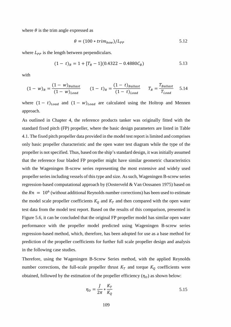
109
where 𝜃𝜃 is the trim angle expressed as
𝜃𝜃 = (100 ∗ 𝐶𝐶𝑡𝑡𝑖𝑖𝑛𝑛𝑏𝑏𝑏𝑏𝑤𝑤)/𝐿𝐿𝑃𝑃𝑃𝑃 5.12
where 𝐿𝐿𝑃𝑃𝑃𝑃 is the length between perpendiculars.
(1 − 𝐶𝐶)𝑅𝑅 = 1 + [𝑃𝑃𝑅𝑅 − 1](0.4322 − 0.4880𝐶𝐶𝐵𝐵) 5.13
with
(1 − 𝑤𝑤)𝑅𝑅 =(1 − 𝑤𝑤)𝐵𝐵𝑔𝑔𝑙𝑙𝑙𝑙𝑔𝑔𝑔𝑔𝐴𝐴(1 − 𝑤𝑤)𝑊𝑊𝑏𝑏𝑔𝑔𝐴𝐴
(1 − 𝐶𝐶)𝑅𝑅 =(1 − 𝐶𝐶)𝐵𝐵𝑔𝑔𝑙𝑙𝑙𝑙𝑔𝑔𝑔𝑔𝐴𝐴(1 − 𝐶𝐶)𝑊𝑊𝑏𝑏𝑔𝑔𝐴𝐴
𝑃𝑃𝑅𝑅 =𝑃𝑃𝐵𝐵𝑔𝑔𝑙𝑙𝑙𝑙𝑔𝑔𝑔𝑔𝐴𝐴𝑃𝑃𝑊𝑊𝑏𝑏𝑔𝑔𝐴𝐴
5.14
where (1 − 𝐶𝐶)𝑊𝑊𝑏𝑏𝑔𝑔𝐴𝐴 and (1 − 𝑤𝑤)𝑊𝑊𝑏𝑏𝑔𝑔𝐴𝐴 are calculated using the Holtrop and Mennen
approach.
As outlined in Chapter 4, the reference products tanker was originally fitted with the
standard fixed pitch (FP) propeller, where the basic design parameters are listed in Table
4.1. The fixed pitch propeller data provided in the model test report is limited and comprises
only basic propeller characteristic and the open water test diagram while the type of the
propeller is not specified. Thus, based on the ship’s standard design, it was initially assumed
that the reference four bladed FP propeller might have similar geometric characteristics
with the Wageningen B-screw series representing the most extensive and widely used
propeller series including vessels of this type and size. As such, Wageningen B-screw series
regression-based computational approach by (Oosterveld & Van Oossanen 1975) based on
the 𝐵𝐵𝑛𝑛 = 106 (without additional Reynolds number corrections) has been used to estimate
the model scale propeller coefficients 𝐾𝐾𝑄𝑄 and 𝐾𝐾𝑇𝑇 and then compared with the open water
test data from the model test report. Based on the results of this comparison, presented in
Figure 5.6, it can be concluded that the original FP propeller model has similar open water
performance with the propeller model predicted using Wageningen B-screw series
regression-based method, which, therefore, has been adopted for use as a base method for
prediction of the propeller coefficients for further full scale propeller design and analysis
in the following case studies.
Therefore, using the Wageningen B-Screw Series method, with the applied Reynolds
number corrections, the full-scale propeller thrust 𝐾𝐾𝑇𝑇 and torque 𝐾𝐾𝑄𝑄 coefficients were
obtained, followed by the estimation of the propeller efficiency (𝜂𝜂𝑂𝑂) as shown below:
𝜂𝜂𝑂𝑂 =𝐽𝐽
2𝜋𝜋∗𝐾𝐾𝑇𝑇𝐾𝐾𝑄𝑄
5.15
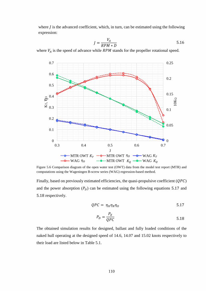
110
where 𝐽𝐽 is the advanced coefficient, which, in turn, can be estimated using the following expression:
𝐽𝐽 =𝑁𝑁𝐴𝐴
𝐵𝐵𝑃𝑃𝑁𝑁 ∗ 𝐷𝐷 5.16
where 𝑁𝑁𝐴𝐴 is the speed of advance while 𝐵𝐵𝑃𝑃𝑁𝑁 stands for the propeller rotational speed.
Figure 5.6 Comparison diagram of the open water test (OWT) data from the model test report (MTR) and computations using the Wageningen B-screw series (WAG) regression-based method.
Finally, based on previously estimated efficiencies, the quasi-propulsive coefficient (𝑄𝑄𝑃𝑃𝐶𝐶)
and the power absorption (𝑃𝑃𝐷𝐷) can be estimated using the following equations 5.17 and
5.18 respectively.
𝑄𝑄𝑃𝑃𝐶𝐶 = 𝜂𝜂𝐻𝐻𝜂𝜂𝑅𝑅𝜂𝜂𝑂𝑂 5.17
𝑃𝑃𝐷𝐷 =𝑃𝑃𝐸𝐸𝑄𝑄𝑃𝑃𝐶𝐶
5.18
The obtained simulation results for designed, ballast and fully loaded conditions of the
naked hull operating at the designed speed of 14.6, 14.07 and 15.02 knots respectively to
their load are listed below in Table 5.1.
0
0.05
0.1
0.15
0.2
0.25
0
0.1
0.2
0.3
0.4
0.5
0.6
0.7
0.3 0.4 0.5 0.6 0.7
10K
Q
KT,
ηO
JMTR OWT MTR OWT WAGWAG MTR OWT WAG
𝐾𝐾𝑇𝑇 𝐾𝐾𝑇𝑇𝐾𝐾𝑄𝑄 𝐾𝐾𝑄𝑄 𝜂𝜂𝑂𝑂
𝜂𝜂𝑂𝑂
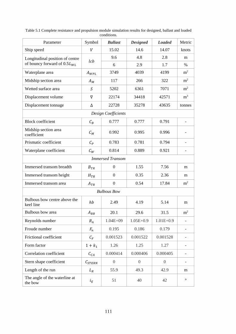
111
Table 5.1 Complete resistance and propulsion module simulation results for designed, ballast and loaded conditions.
Parameter Symbol Ballast Designed Loaded Metric
Ship speed 𝑁𝑁 15.02 14.6 14.07 knots
Longitudinal position of centre of bouncy forward of 0.5𝐿𝐿𝑊𝑊𝑊𝑊 𝑙𝑙𝐶𝐶𝑙𝑙
9.6 4.8 2.8 m
6 2.9 1.7 %
Waterplane area 𝐵𝐵𝑊𝑊𝑃𝑃𝑊𝑊 3749 4039 4199 m2
Midship section area 𝐵𝐵𝑀𝑀 117 266 322 m2
Wetted surface area 𝑆𝑆 5202 6361 7071 m2
Displacement volume ∇ 22174 34418 42571 m3
Displacement tonnage ∆ 22728 35278 43635 tonnes
Design Coefficients
Block coefficient 𝐶𝐶𝐵𝐵 0.777 0.777 0.791 -
Midship section area coefficient 𝐶𝐶𝑀𝑀 0.992 0.995 0.996 -
Prismatic coefficient 𝐶𝐶𝑃𝑃 0.783 0.781 0.794 -
Waterplane coefficient 𝐶𝐶𝑊𝑊 0.814 0.889 0.921 -
Immersed Transom
Immersed transom breadth 𝐵𝐵𝑇𝑇𝑅𝑅 0 1.55 7.56 m
Immersed transom height 𝐻𝐻𝑇𝑇𝑅𝑅 0 0.35 2.36 m
Immersed transom area 𝐵𝐵𝑇𝑇𝑅𝑅 0 0.54 17.84 m2
Bulbous Bow
Bulbous bow centre above the keel line ℎ𝑙𝑙 2.49 4.19 5.14 m
Bulbous bow area 𝐵𝐵𝐵𝐵𝐵𝐵 20.1 29.6 31.5 m2
Reynolds number 𝐵𝐵𝐴𝐴 1.04E+09 1.05E+0.9 1.01E+0.9 -
Froude number 𝑆𝑆𝐴𝐴 0.195 0.186 0.179 -
Frictional coefficient 𝐶𝐶𝐹𝐹 0.001523 0.001522 0.001528 -
Form factor 1 + 𝑘𝑘1 1.26 1.25 1.27 -
Correlation coefficient 𝐶𝐶𝐶𝐶𝐴𝐴 0.000414 0.000406 0.000405 -
Stern shape coefficient 𝐶𝐶𝑆𝑆𝑇𝑇𝐸𝐸𝑅𝑅𝑆𝑆 0 0 0 -
Length of the run 𝐿𝐿𝑅𝑅 55.9 49.3 42.9 m
The angle of the waterline at the bow 𝑖𝑖𝐸𝐸 51 40 42 °
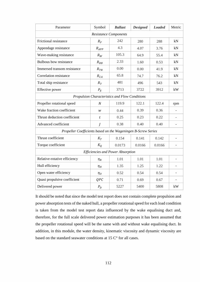
112
Parameter Symbol Ballast Designed Loaded Metric
Resistance Components
Frictional resistance 𝐵𝐵𝐹𝐹 242 280 288 kN
Appendage resistance 𝐵𝐵𝐴𝐴𝑃𝑃𝑃𝑃 4.3 4.07 3.76 kN
Wave-making resistance 𝐵𝐵𝑊𝑊 105.3 64.9 55.4 kN
Bulbous bow resistance 𝐵𝐵𝐵𝐵𝐵𝐵 2.33 1.60 0.53 kN
Immersed transom resistance 𝐵𝐵𝑇𝑇𝑅𝑅 0.00 0.00 41.9 kN
Correlation resistance 𝐵𝐵𝐶𝐶𝐴𝐴 65.8 74.7 76.2 kN
Total ship resistance 𝐵𝐵𝑇𝑇 481 496 543 kN
Effective power 𝑃𝑃𝐸𝐸 3713 3722 3912 kW
Propulsion Characteristics and Flow Conditions
Propeller rotational speed 𝑁𝑁 119.9 122.1 122.4 rpm
Wake fraction coefficient 𝑤𝑤 0.44 0.39 0.36 -
Thrust deduction coefficient 𝐶𝐶 0.25 0.23 0.22 -
Advanced coefficient 𝐽𝐽 0.38 0.40 0.40 -
Propeller Coefficients based on the Wageningen B-Screw Series
Thrust coefficient 𝐾𝐾𝑇𝑇 0.154 0.141 0.142 -
Torque coefficient 𝐾𝐾𝑄𝑄 0.0173 0.0166 0.0166 -
Efficiencies and Power Absorption
Relative-rotative efficiency 𝜂𝜂𝑅𝑅 1.01 1.01 1.01 -
Hull efficiency 𝜂𝜂𝐻𝐻 1.35 1.25 1.22 -
Open water efficiency 𝜂𝜂𝑂𝑂 0.52 0.54 0.54 -
Quasi propulsive coefficient 𝑄𝑄𝑃𝑃𝐶𝐶 0.71 0.69 0.67 -
Delivered power 𝑃𝑃𝐷𝐷 5227 5400 5808 kW
It should be noted that since the model test report does not contain complete propulsion and
power absorption tests of the naked hull, a propeller rotational speed for each load condition
is taken from the model test report data influenced by the wake equalising duct and,
therefore, for the full scale delivered power estimation purposes it has been assumed that
the propeller rotational speed will be the same with and without wake equalising duct. In
addition, in this module, the water density, kinematic viscosity and dynamic viscosity are
based on the standard seawater conditions at 15 C° for all cases.
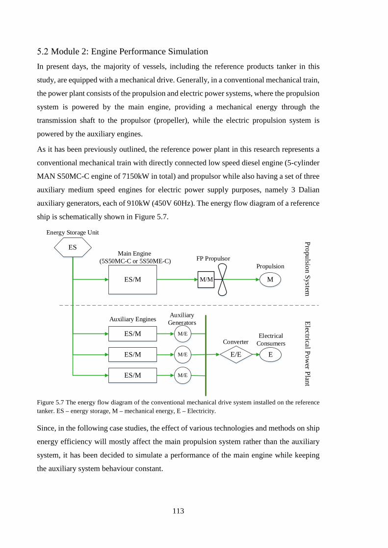
113
Module 2: Engine Performance Simulation In present days, the majority of vessels, including the reference products tanker in this
study, are equipped with a mechanical drive. Generally, in a conventional mechanical train,
the power plant consists of the propulsion and electric power systems, where the propulsion
system is powered by the main engine, providing a mechanical energy through the
transmission shaft to the propulsor (propeller), while the electric propulsion system is
powered by the auxiliary engines.
As it has been previously outlined, the reference power plant in this research represents a
conventional mechanical train with directly connected low speed diesel engine (5-cylinder
MAN S50MC-C engine of 7150kW in total) and propulsor while also having a set of three
auxiliary medium speed engines for electric power supply purposes, namely 3 Dalian
auxiliary generators, each of 910kW (450V 60Hz). The energy flow diagram of a reference
ship is schematically shown in Figure 5.7.
Energy Storage Unit
Main Engine (5S50MC-C or 5S50ME-C)
Auxiliary Engines
FP PropulsorPropulsion
Auxiliary Generators
ConverterElectrical
Consumers
Propulsion SystemElectrical Pow
er Plant
ES
ES/M M/M M
ES/M
ES/M
ES/M
E
M/E
M/E
M/E
E/E
Figure 5.7 The energy flow diagram of the conventional mechanical drive system installed on the reference tanker. ES – energy storage, M – mechanical energy, E – Electricity.
Since, in the following case studies, the effect of various technologies and methods on ship
energy efficiency will mostly affect the main propulsion system rather than the auxiliary
system, it has been decided to simulate a performance of the main engine while keeping
the auxiliary system behaviour constant.
114
There are several methods available to predict a performance of the marine diesel engine
including CFD simulation, multi-zone simulation models and a look-up table approach.
• CFD simulations The CFD-based simulations, such as the model of large 2-stroke marine diesel engine
outlined in (Jin & Vassalos 2013) that has been developed and validated using CFD
computational approach, can be used to understand and analyse the combustion process in
great details. For instance, the (Jin & Vassalos 2013) model consists of the RNG (Re-
Normalisation Group) k-ε turbulence simulation component, aimed to capture the in-
cylinder flow compression and mixing, and the combustion simulation model based on the
finite-rate approach designed to simulate the chemical reactions while taking into account
the turbulence effect on the combustion processes. However, at the current stage, such
models are only able to simulate the combustion process but not calculate the engine fuel
consumption while the requirements from the model in terms of the level of details are
high. In addition, such simulations do not include the effect of the turbocharger.
• Multi-zone engine simulations The multi-zone engine simulation models, including the early work by (Banisoleiman et al.
n.d.) and recent NTUA Engine Performance and Emissions code developed by (Hountalas
et al. 2013), are purely based on thermodynamics which allows a detailed analysis of the
engine performance of both 2- and 4-stroke diesel engines as well as to predict the level of
atmospheric emissions. Both models allow to adjust the injection and combustion profiles,
namely to modify pressure, temperature, injection angle and gas composition in order to
uncover the principal forces affecting the efficiency and emissions profile. However, for
the simulation purposes, it is required to provide an extensive engine geometry, as well as
the initial fuel consumption rate, power output values for each load and other supporting
information which are not always available and in some cases remain confidential to the
manufacturer. Moreover, in terms of this research, the fuel consumption rate is one of the
energy efficiency indicators (EEI) and needs to be predicted by this module in order to be
able to estimate the effect of certain energy efficiency innovation on the ship’s overall
efficiency level.
• Look-up table approach The lookup-table approach is a fast and accurate method while its applicability is strongly
restricted by the availability of required information. For instance, an open source
Computational Engine Application System (CEAS) engine calculation tool developed by

115
MAN has an extensive engine performance database including the Tier III engines and
innovative fuels such as methane, ethane, LPG and methanol. The model allows choosing
preferable types of the turbocharger, to modify engine cooling system as well as to specify
the ambient conditions, propeller type and the fuel sulphur content. The CEAS engine
calculation tool also provides a user with the engine layout diagram option to choose the
required power and rotational speed in accordance with the permitted values. As such, the
CEAS is able to calculate the power, rotational speed, SFOC, exhaust gas flow, exhaust
gas temperature and even the potential steam production capacity for each load. However,
this model does not calculate the exhaust emissions level neither does it provide any
insights on the engine inner behaviour.
Since the reference ship is already equipped with the MAN low-speed diesel engine, plus
the main purpose of this engine simulation module is to help to evaluate and compare the
effect of a particular energy efficiency-enhancing technology, or method as a part of the
holistic ship simulation analysis rather than looking deeply into the engine behaviour itself,
the CEAS engine calculation tool has been selected as an engine simulation module.
However, this tool does not predict the atmospheric emissions level meaning that the
additional emissions prediction model has been separately developed and outlined in the
next section.
The CEAS database has recently been updated with the Tier III engines data while the
entire Tier I engines data (the mechanical MC/MC-C range) has been removed. At the same
time, according to the entry in the register book, the examinee oil products tanker is
equipped with the Tier I mechanically controlled MC/MC-C (5S50MC-C) engine. Hence,
since the Tier I engines do not comply with the modern regulations while this research is
dedicated to the future developments, the main reference MC/MC-C engine has been
switched to the electronically controlled ME/ME-C engine (5S50ME-C) of the same size
which complies with the Tier II regulations. It is important to note that MC/MC-C engines
still can achieve the Tier II requirements by introducing new fuel system components such
as plunger/barrel and fuel valve nozzles as well as by an adjustment of the combustion
chamber volume by piston rod shims, the scavenge air pressure and the exhaust cam profile
(MAN Diesel and Turbo 2014a). However, the electronically controlled ME/ME-C engines
have a major advantage with respect to operating at even very low load for long periods of
time, whilst offering a substantial reduction in fuel oil consumption compared to MC/MC-
C engines at such low loads possible due to an adjustment of the programming of the
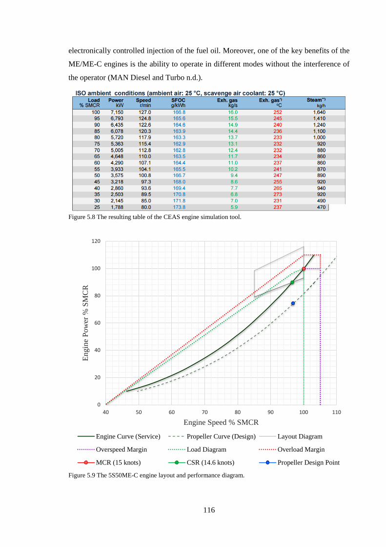
116
electronically controlled injection of the fuel oil. Moreover, one of the key benefits of the
ME/ME-C engines is the ability to operate in different modes without the interference of
the operator (MAN Diesel and Turbo n.d.).
Figure 5.8 The resulting table of the CEAS engine simulation tool.
Figure 5.9 The 5S50ME-C engine layout and performance diagram.
0
20
40
60
80
100
120
40 50 60 70 80 90 100 110
Engi
ne P
ower
% S
MC
R
Engine Speed % SMCR
Engine Curve (Service) Propeller Curve (Design) Layout Diagram
Overspeed Margin Load Diagram Overload Margin
MCR (15 knots) CSR (14.6 knots) Propeller Design Point
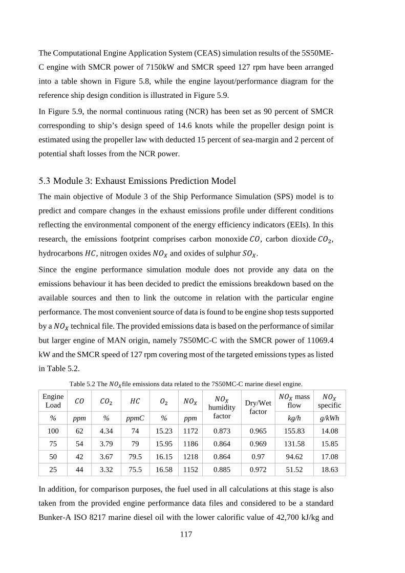
117
The Computational Engine Application System (CEAS) simulation results of the 5S50ME-
C engine with SMCR power of 7150kW and SMCR speed 127 rpm have been arranged
into a table shown in Figure 5.8, while the engine layout/performance diagram for the
reference ship design condition is illustrated in Figure 5.9.
In Figure 5.9, the normal continuous rating (NCR) has been set as 90 percent of SMCR
corresponding to ship’s design speed of 14.6 knots while the propeller design point is
estimated using the propeller law with deducted 15 percent of sea-margin and 2 percent of
potential shaft losses from the NCR power.
Module 3: Exhaust Emissions Prediction Model The main objective of Module 3 of the Ship Performance Simulation (SPS) model is to
predict and compare changes in the exhaust emissions profile under different conditions
reflecting the environmental component of the energy efficiency indicators (EEIs). In this
research, the emissions footprint comprises carbon monoxide 𝐶𝐶𝐶𝐶, carbon dioxide 𝐶𝐶𝐶𝐶2,
hydrocarbons 𝐻𝐻𝐶𝐶, nitrogen oxides 𝑁𝑁𝐶𝐶𝑋𝑋 and oxides of sulphur 𝑆𝑆𝐶𝐶𝑋𝑋.
Since the engine performance simulation module does not provide any data on the
emissions behaviour it has been decided to predict the emissions breakdown based on the
available sources and then to link the outcome in relation with the particular engine
performance. The most convenient source of data is found to be engine shop tests supported
by a 𝑁𝑁𝐶𝐶𝑋𝑋 technical file. The provided emissions data is based on the performance of similar
but larger engine of MAN origin, namely 7S50MC-C with the SMCR power of 11069.4
kW and the SMCR speed of 127 rpm covering most of the targeted emissions types as listed
in Table 5.2.
Table 5.2 The 𝑁𝑁𝐶𝐶𝑋𝑋file emissions data related to the 7S50MC-C marine diesel engine.
Engine Load 𝐶𝐶𝐶𝐶 𝐶𝐶𝐶𝐶2 𝐻𝐻𝐶𝐶 𝐶𝐶2 𝑁𝑁𝐶𝐶𝑋𝑋 𝑁𝑁𝐶𝐶𝑋𝑋
humidity factor
Dry/Wet factor
𝑁𝑁𝐶𝐶𝑋𝑋 mass flow
𝑁𝑁𝐶𝐶𝑋𝑋 specific
% ppm % ppmC % ppm kg/h g/kWh
100 62 4.34 74 15.23 1172 0.873 0.965 155.83 14.08
75 54 3.79 79 15.95 1186 0.864 0.969 131.58 15.85
50 42 3.67 79.5 16.15 1218 0.864 0.97 94.62 17.08
25 44 3.32 75.5 16.58 1152 0.885 0.972 51.52 18.63
In addition, for comparison purposes, the fuel used in all calculations at this stage is also
taken from the provided engine performance data files and considered to be a standard
Bunker-A ISO 8217 marine diesel oil with the lower calorific value of 42,700 kJ/kg and
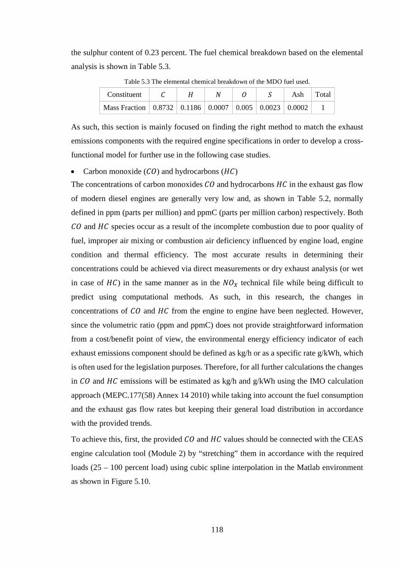
118
the sulphur content of 0.23 percent. The fuel chemical breakdown based on the elemental
analysis is shown in Table 5.3.
Table 5.3 The elemental chemical breakdown of the MDO fuel used.
Constituent 𝐶𝐶 𝐻𝐻 𝑁𝑁 𝐶𝐶 𝑆𝑆 Ash Total
Mass Fraction 0.8732 0.1186 0.0007 0.005 0.0023 0.0002 1
As such, this section is mainly focused on finding the right method to match the exhaust
emissions components with the required engine specifications in order to develop a cross-
functional model for further use in the following case studies.
• Carbon monoxide (𝐶𝐶𝐶𝐶) and hydrocarbons (𝐻𝐻𝐶𝐶) The concentrations of carbon monoxides 𝐶𝐶𝐶𝐶 and hydrocarbons 𝐻𝐻𝐶𝐶 in the exhaust gas flow
of modern diesel engines are generally very low and, as shown in Table 5.2, normally
defined in ppm (parts per million) and ppmC (parts per million carbon) respectively. Both
𝐶𝐶𝐶𝐶 and 𝐻𝐻𝐶𝐶 species occur as a result of the incomplete combustion due to poor quality of
fuel, improper air mixing or combustion air deficiency influenced by engine load, engine
condition and thermal efficiency. The most accurate results in determining their
concentrations could be achieved via direct measurements or dry exhaust analysis (or wet
in case of 𝐻𝐻𝐶𝐶) in the same manner as in the 𝑁𝑁𝐶𝐶𝑋𝑋 technical file while being difficult to
predict using computational methods. As such, in this research, the changes in
concentrations of 𝐶𝐶𝐶𝐶 and 𝐻𝐻𝐶𝐶 from the engine to engine have been neglected. However,
since the volumetric ratio (ppm and ppmC) does not provide straightforward information
from a cost/benefit point of view, the environmental energy efficiency indicator of each
exhaust emissions component should be defined as kg/h or as a specific rate g/kWh, which
is often used for the legislation purposes. Therefore, for all further calculations the changes
in 𝐶𝐶𝐶𝐶 and 𝐻𝐻𝐶𝐶 emissions will be estimated as kg/h and g/kWh using the IMO calculation
approach (MEPC.177(58) Annex 14 2010) while taking into account the fuel consumption
and the exhaust gas flow rates but keeping their general load distribution in accordance
with the provided trends.
To achieve this, first, the provided 𝐶𝐶𝐶𝐶 and 𝐻𝐻𝐶𝐶 values should be connected with the CEAS
engine calculation tool (Module 2) by “stretching” them in accordance with the required
loads (25 – 100 percent load) using cubic spline interpolation in the Matlab environment
as shown in Figure 5.10.
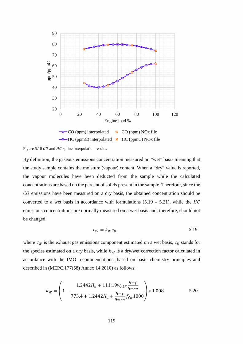
119
Figure 5.10 𝐶𝐶𝐶𝐶 and 𝐻𝐻𝐶𝐶 spline interpolation results.
By definition, the gaseous emissions concentration measured on “wet” basis meaning that
the study sample contains the moisture (vapour) content. When a “dry” value is reported,
the vapour molecules have been deducted from the sample while the calculated
concentrations are based on the percent of solids present in the sample. Therefore, since the
𝐶𝐶𝐶𝐶 emissions have been measured on a dry basis, the obtained concentration should be
converted to a wet basis in accordance with formulations (5.19 – 5.21), while the 𝐻𝐻𝐶𝐶
emissions concentrations are normally measured on a wet basis and, therefore, should not
be changed.
𝐶𝐶𝑊𝑊 = 𝑘𝑘𝑊𝑊𝐶𝐶𝐷𝐷 5.19
where 𝐶𝐶𝑊𝑊 is the exhaust gas emissions component estimated on a wet basis, 𝐶𝐶𝐷𝐷 stands for
the species estimated on a dry basis, while 𝑘𝑘𝑊𝑊 is a dry/wet correction factor calculated in
accordance with the IMO recommendations, based on basic chemistry principles and
described in (MEPC.177(58) Annex 14 2010) as follows:
𝑘𝑘𝑊𝑊 = 1 −1.2442𝐻𝐻𝑔𝑔 + 111.19𝑤𝑤𝐴𝐴𝑊𝑊𝐹𝐹
𝑞𝑞𝑚𝑚𝑟𝑟𝑞𝑞𝑚𝑚𝑔𝑔𝐴𝐴
773.4 + 1.2442𝐻𝐻𝑔𝑔 +𝑞𝑞𝑚𝑚𝑟𝑟𝑞𝑞𝑚𝑚𝑔𝑔𝐴𝐴
𝑓𝑓𝑟𝑟𝑤𝑤1000 ∗ 1.008 5.20
20
30
40
50
60
70
80
90
0 20 40 60 80 100 120
ppm
/ppm
C
Engine load %
CO (ppm) interpolated CO (ppm) NOx fileHC (ppmC) interpolated HC (ppmC) NOx file
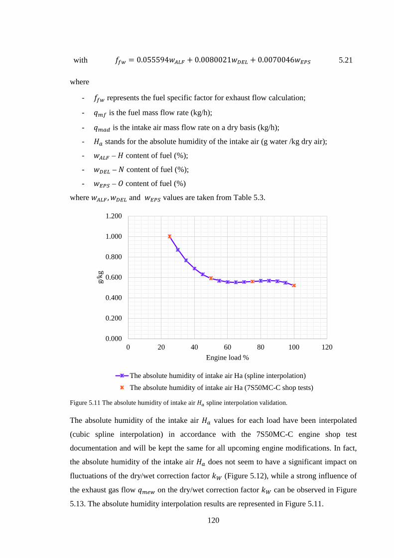
120
with 𝑓𝑓𝑟𝑟𝑤𝑤 = 0.055594𝑤𝑤𝐴𝐴𝑊𝑊𝐹𝐹 + 0.0080021𝑤𝑤𝐷𝐷𝐸𝐸𝑊𝑊 + 0.0070046𝑤𝑤𝐸𝐸𝑃𝑃𝑆𝑆 5.21
where
- 𝑓𝑓𝑟𝑟𝑤𝑤 represents the fuel specific factor for exhaust flow calculation;
- 𝑞𝑞𝑚𝑚𝑟𝑟 is the fuel mass flow rate (kg/h);
- 𝑞𝑞𝑚𝑚𝑔𝑔𝐴𝐴 is the intake air mass flow rate on a dry basis (kg/h);
- 𝐻𝐻𝑔𝑔 stands for the absolute humidity of the intake air (g water /kg dry air);
- 𝑤𝑤𝐴𝐴𝑊𝑊𝐹𝐹 – 𝐻𝐻 content of fuel (%);
- 𝑤𝑤𝐷𝐷𝐸𝐸𝑊𝑊 – 𝑁𝑁 content of fuel (%);
- 𝑤𝑤𝐸𝐸𝑃𝑃𝑆𝑆 – 𝐶𝐶 content of fuel (%)
where 𝑤𝑤𝐴𝐴𝑊𝑊𝐹𝐹 ,𝑤𝑤𝐷𝐷𝐸𝐸𝑊𝑊 and 𝑤𝑤𝐸𝐸𝑃𝑃𝑆𝑆 values are taken from Table 5.3.
Figure 5.11 The absolute humidity of intake air 𝐻𝐻𝑔𝑔 spline interpolation validation.
The absolute humidity of the intake air 𝐻𝐻𝑔𝑔 values for each load have been interpolated
(cubic spline interpolation) in accordance with the 7S50MC-C engine shop test
documentation and will be kept the same for all upcoming engine modifications. In fact,
the absolute humidity of the intake air 𝐻𝐻𝑔𝑔 does not seem to have a significant impact on
fluctuations of the dry/wet correction factor 𝑘𝑘𝑊𝑊 (Figure 5.12), while a strong influence of
the exhaust gas flow 𝑞𝑞𝑚𝑚𝐴𝐴𝑤𝑤 on the dry/wet correction factor 𝑘𝑘𝑊𝑊 can be observed in Figure
5.13. The absolute humidity interpolation results are represented in Figure 5.11.
0.000
0.200
0.400
0.600
0.800
1.000
1.200
0 20 40 60 80 100 120
g/kg
Engine load %
The absolute humidity of intake air Ha (spline interpolation)The absolute humidity of intake air Ha (7S50MC-C shop tests)
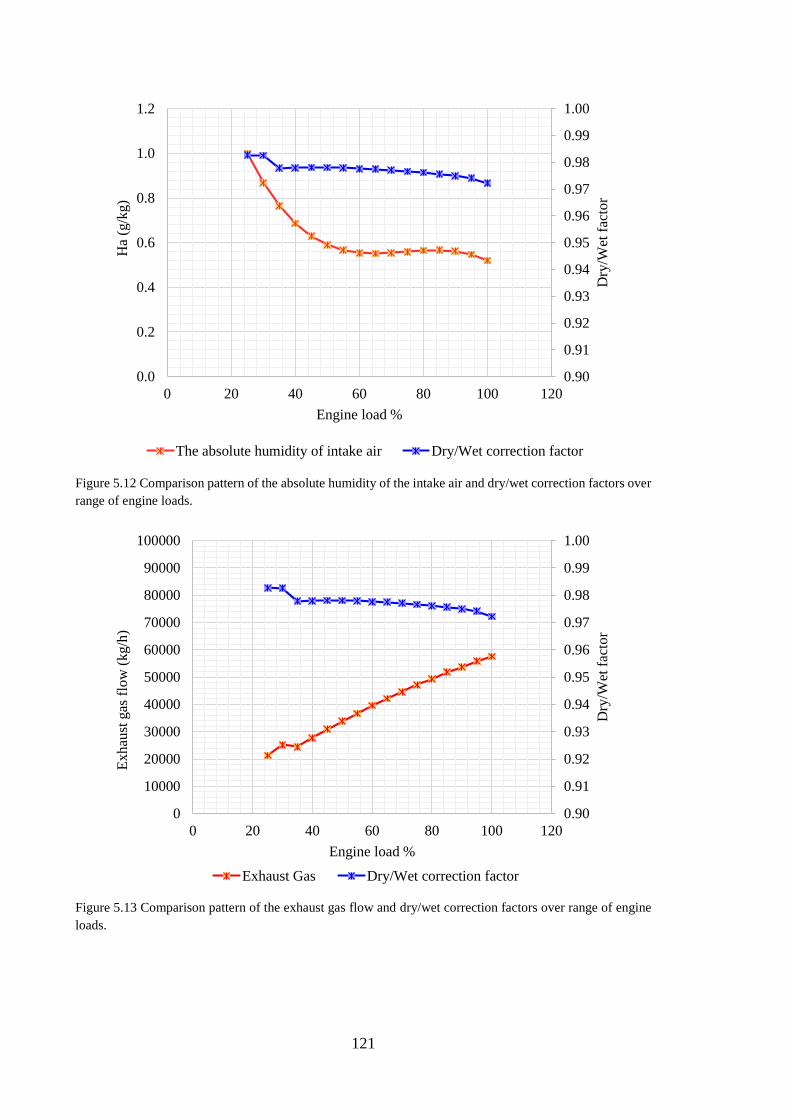
121
Figure 5.12 Comparison pattern of the absolute humidity of the intake air and dry/wet correction factors over range of engine loads.
Figure 5.13 Comparison pattern of the exhaust gas flow and dry/wet correction factors over range of engine loads.
0.90
0.91
0.92
0.93
0.94
0.95
0.96
0.97
0.98
0.99
1.00
0.0
0.2
0.4
0.6
0.8
1.0
1.2
0 20 40 60 80 100 120
Dry
/Wet
fact
or
Ha
(g/k
g)
Engine load %
The absolute humidity of intake air Dry/Wet correction factor
0.90
0.91
0.92
0.93
0.94
0.95
0.96
0.97
0.98
0.99
1.00
0
10000
20000
30000
40000
50000
60000
70000
80000
90000
100000
0 20 40 60 80 100 120
Dry
/Wet
fact
or
Exha
ust g
as fl
ow (k
g/h)
Engine load %
Exhaust Gas Dry/Wet correction factor
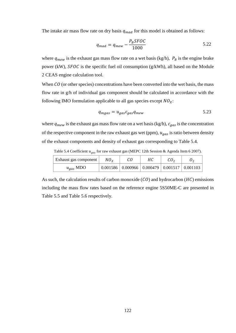
122
The intake air mass flow rate on dry basis 𝑞𝑞𝑚𝑚𝑔𝑔𝐴𝐴 for this model is obtained as follows:
𝑞𝑞𝑚𝑚𝑔𝑔𝐴𝐴 = 𝑞𝑞𝑚𝑚𝐴𝐴𝑤𝑤 −𝑃𝑃𝐵𝐵𝑆𝑆𝑆𝑆𝐶𝐶𝐶𝐶
1000 5.22
where 𝑞𝑞𝑚𝑚𝐴𝐴𝑤𝑤 is the exhaust gas mass flow rate on a wet basis (kg/h), 𝑃𝑃𝐵𝐵 is the engine brake
power (kW), 𝑆𝑆𝑆𝑆𝐶𝐶𝐶𝐶 is the specific fuel oil consumption (g/kWh), all based on the Module
2 CEAS engine calculation tool.
When 𝐶𝐶𝐶𝐶 (or other species) concentrations have been converted into the wet basis, the mass
flow rate in g/h of individual gas component should be calculated in accordance with the
following IMO formulation applicable to all gas species except 𝑁𝑁𝐶𝐶𝑋𝑋:
𝑞𝑞𝑚𝑚𝑔𝑔𝑔𝑔𝑔𝑔 = 𝑢𝑢𝑔𝑔𝑔𝑔𝑔𝑔𝐶𝐶𝑔𝑔𝑔𝑔𝑔𝑔𝑞𝑞𝑚𝑚𝐴𝐴𝑤𝑤 5.23
where 𝑞𝑞𝑚𝑚𝐴𝐴𝑤𝑤 is the exhaust gas mass flow rate on a wet basis (kg/h), 𝐶𝐶𝑔𝑔𝑔𝑔𝑔𝑔 is the concentration
of the respective component in the raw exhaust gas wet (ppm), 𝑢𝑢𝑔𝑔𝑔𝑔𝑔𝑔 is ratio between density
of the exhaust components and density of exhaust gas corresponding to Table 5.4.
Table 5.4 Coefficient 𝑢𝑢𝑔𝑔𝐻𝐻𝑔𝑔 for raw exhaust gas (MEPC 12th Session & Agenda Item 6 2007).
Exhaust gas component 𝑁𝑁𝐶𝐶𝑋𝑋 𝐶𝐶𝐶𝐶 𝐻𝐻𝐶𝐶 𝐶𝐶𝐶𝐶2 𝐶𝐶2
𝑢𝑢𝑔𝑔𝑔𝑔𝑔𝑔 MDO 0.001586 0.000966 0.000479 0.001517 0.001103
As such, the calculation results of carbon monoxide (𝐶𝐶𝐶𝐶) and hydrocarbon (𝐻𝐻𝐶𝐶) emissions
including the mass flow rates based on the reference engine 5S50ME-C are presented in
Table 5.5 and Table 5.6 respectively.
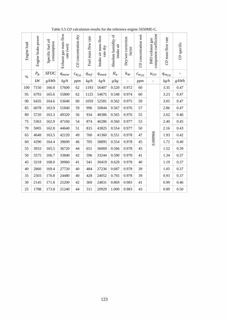
123
Table 5.5 𝐶𝐶𝐶𝐶 calculation results for the reference engine 5S50ME-C. En
gine
load
Engi
ne b
rake
pow
er
Spec
ific
fuel
oil
cons
umpt
ion
Exha
ust g
as m
ass f
low
ra
te (w
et)
𝐶𝐶𝐶𝐶 c
once
ntra
tion
dry
Fuel
mas
s flo
w ra
te
Inta
ke a
ir m
ass f
low
ra
te d
ry
Abs
olut
e hu
mid
ity o
f in
take
air
Dry
/wet
cor
rect
ion
fact
or
𝐶𝐶𝐶𝐶 c
once
ntra
tion
wet
IMO
exh
aust
gas
co
mpo
nent
coe
ffic
ient
𝐶𝐶𝐶𝐶 m
ass f
low
rate
𝐶𝐶𝐶𝐶 sp
ecifi
c
% 𝑃𝑃𝐵𝐵 SFOC 𝑞𝑞𝑚𝑚𝐴𝐴𝑤𝑤 𝐶𝐶𝐴𝐴𝐶𝐶𝐶𝐶 𝑞𝑞𝑚𝑚𝑟𝑟 𝑞𝑞𝑚𝑚𝑔𝑔𝐴𝐴 𝐻𝐻𝑔𝑔 𝑘𝑘𝑊𝑊 𝐶𝐶𝑤𝑤𝐶𝐶𝐶𝐶 𝑢𝑢𝐶𝐶𝑂𝑂 𝑞𝑞𝑚𝑚𝐶𝐶𝐶𝐶 -
kW g/kWh kg/h ppm kg/h kg/h g/kg - ppm - kg/h g/kWh
100 7150 166.8 57600 62 1193 56407 0.520 0.972 60
0.00
0966
3.35 0.47
95 6793 165.6 55800 62 1125 54675 0.548 0.974 60 3.23 0.47
90 6435 164.6 53640 60 1059 52581 0.562 0.975 59 3.05 0.47
85 6078 163.9 51840 59 996 50844 0.567 0.976 57 2.86 0.47
80 5720 163.3 49320 56 934 48386 0.565 0.976 55 2.62 0.46
75 5363 162.9 47160 54 874 46286 0.560 0.977 53 2.40 0.45
70 5005 162.8 44640 51 815 43825 0.554 0.977 50 2.16 0.43
65 4648 163.5 42120 49 760 41360 0.551 0.978 47 1.93 0.42
60 4290 164.4 39600 46 705 38895 0.554 0.978 45 1.72 0.40
55 3933 165.5 36720 44 651 36069 0.566 0.978 43 1.52 0.39
50 3575 166.7 33840 42 596 33244 0.590 0.978 41 1.34 0.37
45 3218 168.0 30960 41 541 30419 0.629 0.978 40 1.19 0.37
40 2860 169.4 27720 40 484 27236 0.687 0.978 39 1.05 0.37
35 2503 170.8 24480 40 428 24052 0.765 0.978 39 0.93 0.37
30 2145 171.8 25200 42 369 24831 0.869 0.983 41 0.99 0.46
25 1788 173.8 21240 44 311 20929 1.000 0.983 43 0.89 0.50
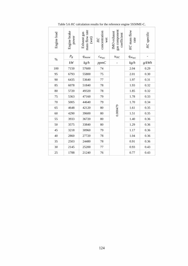
124
Table 5.6 𝐻𝐻𝐶𝐶 calculation results for the reference engine 5S50ME-C.
Engi
ne lo
ad
Engi
ne b
rake
po
wer
Exha
ust g
as
mas
s flo
w ra
te
(wet
)
𝐻𝐻𝐶𝐶
conc
entra
tion
wet
IMO
exh
aust
ga
s com
pone
nt
coef
ficie
nt
𝐻𝐻𝐶𝐶
mas
s flo
w
rate
𝐻𝐻𝐶𝐶
spec
ific
% 𝑃𝑃𝐵𝐵 𝑞𝑞𝑚𝑚𝐴𝐴𝑤𝑤 𝐶𝐶𝑤𝑤𝐻𝐻𝐶𝐶 𝑢𝑢𝐻𝐻𝐶𝐶 𝑞𝑞𝑚𝑚𝐻𝐻𝐶𝐶 -
kW kg/h ppmC - kg/h g/kWh 100 7150 57600 74
0.00
0479
2.04 0.29
95 6793 55800 75 2.01 0.30
90 6435 53640 77 1.97 0.31
85 6078 51840 78 1.93 0.32
80 5720 49320 78 1.85 0.32
75 5363 47160 79 1.78 0.33
70 5005 44640 79 1.70 0.34
65 4648 42120 80 1.61 0.35
60 4290 39600 80 1.51 0.35
55 3933 36720 80 1.40 0.36
50 3575 33840 80 1.29 0.36
45 3218 30960 79 1.17 0.36
40 2860 27720 78 1.04 0.36
35 2503 24480 78 0.91 0.36
30 2145 25200 77 0.93 0.43
25 1788 21240 76 0.77 0.43

125
• Carbon dioxide (𝐶𝐶𝐶𝐶2) Since the concentrations of 𝐶𝐶𝐶𝐶2 in the raw exhaust flow is much higher than of other
species, it is important to address their fluctuations when considering different engines in
addition to changes associated with the fuel consumption rate. In fact, the measured
concentrations of 𝐶𝐶𝐶𝐶2 in the dry exhaust are normally described in a form of percentage
(%) rather than using a volumetric expression (ppm).
With respect to predictions of the 𝐶𝐶𝐶𝐶2 concentrations, since the 𝐶𝐶𝐶𝐶2 emissions are directly
linked with fuel consumption and fuel composition, it was decided to incorporate a carbon
balance method. This method is based on basic chemistry principles and adopted by IMO
as one step calculation procedure recommended for the prediction of exhaust gas mass flow
in accordance with fuel consumption, fuel composition and the exhaust gas concentrations
using the formulations (5.24), (5.25) and (5.26) (MEPC.177(58) Annex 14 2010).
Moreover, the idea is to convert this formula into an equation targeting the prediction of
the 𝐶𝐶𝐶𝐶2 concentrations on a dry basis (𝐶𝐶𝐶𝐶𝑂𝑂2𝐴𝐴) while the exhaust gas mass flow rate (𝑞𝑞𝑚𝑚𝐴𝐴𝑤𝑤)
as well as the fuel consumption (𝑞𝑞𝑚𝑚𝑟𝑟) should be estimated using the engine simulation
module. This will help in establishing a continuous relationship between the fuel
consumption required under certain conditions in the following case studies (Chapters 7-
11) and the fluctuations of the 𝐶𝐶𝐶𝐶2 emissions concentrations associated with it.
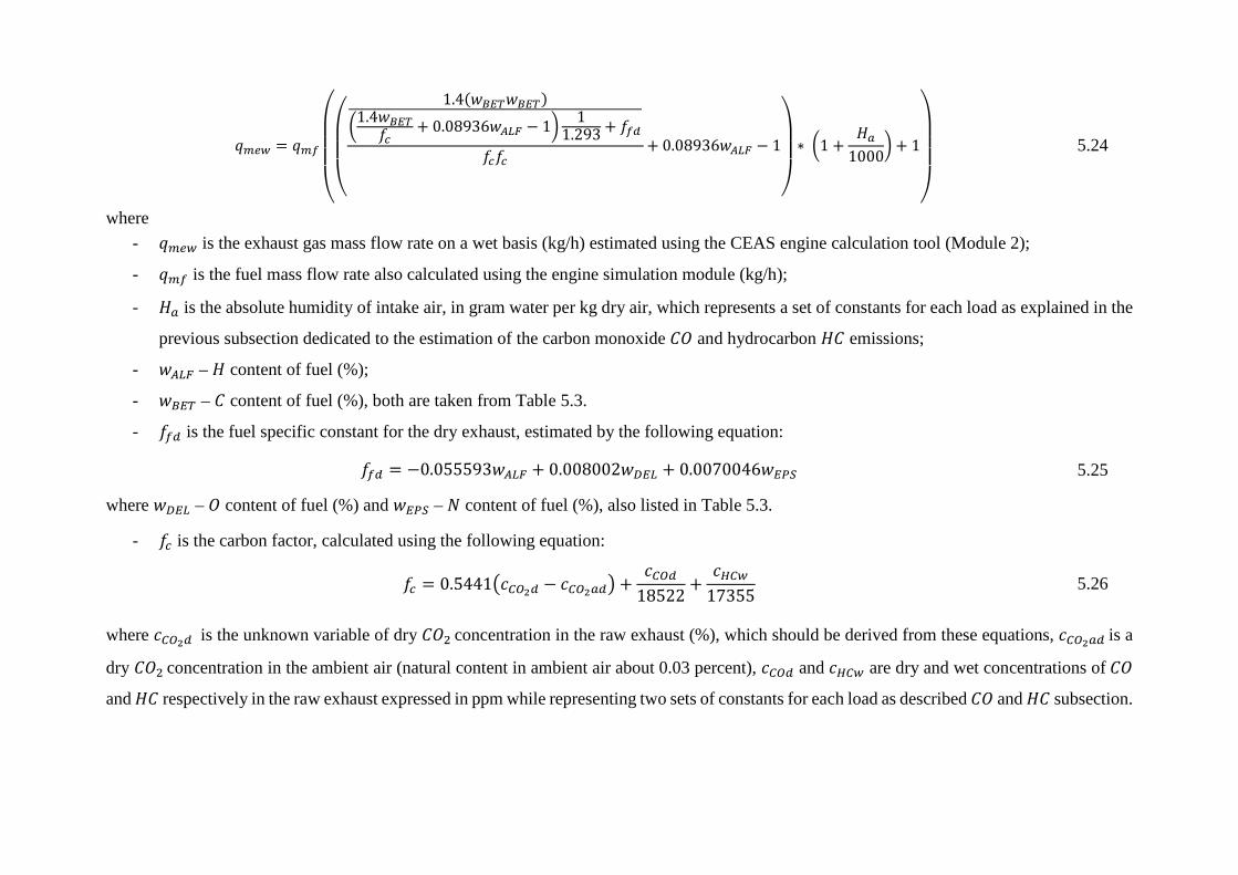
q𝑞𝑞𝑚𝑚𝐴𝐴𝑤𝑤 = 𝑞𝑞𝑚𝑚𝑟𝑟
⎝
⎜⎜⎜⎛
⎝
⎜⎜⎛
1.4(𝑤𝑤𝐵𝐵𝐸𝐸𝑇𝑇𝑤𝑤𝐵𝐵𝐸𝐸𝑇𝑇)
1.4𝑤𝑤𝐵𝐵𝐸𝐸𝑇𝑇𝑓𝑓𝑐𝑐
+ 0.08936𝑤𝑤𝐴𝐴𝑊𝑊𝐹𝐹 − 1 11.293 + 𝑓𝑓𝑟𝑟𝐴𝐴
𝑓𝑓𝑐𝑐𝑓𝑓𝑐𝑐+ 0.08936𝑤𝑤𝐴𝐴𝑊𝑊𝐹𝐹 − 1
⎠
⎟⎟⎞∗ 1 +
𝐻𝐻𝑔𝑔1000
+ 1
⎠
⎟⎟⎟⎞
5.24
where - 𝑞𝑞𝑚𝑚𝐴𝐴𝑤𝑤 is the exhaust gas mass flow rate on a wet basis (kg/h) estimated using the CEAS engine calculation tool (Module 2);
- 𝑞𝑞𝑚𝑚𝑟𝑟 is the fuel mass flow rate also calculated using the engine simulation module (kg/h);
- 𝐻𝐻𝑔𝑔 is the absolute humidity of intake air, in gram water per kg dry air, which represents a set of constants for each load as explained in the
previous subsection dedicated to the estimation of the carbon monoxide 𝐶𝐶𝐶𝐶 and hydrocarbon 𝐻𝐻𝐶𝐶 emissions;
- 𝑤𝑤𝐴𝐴𝑊𝑊𝐹𝐹 – 𝐻𝐻 content of fuel (%);
- 𝑤𝑤𝐵𝐵𝐸𝐸𝑇𝑇 – 𝐶𝐶 content of fuel (%), both are taken from Table 5.3.
- 𝑓𝑓𝑟𝑟𝐴𝐴 is the fuel specific constant for the dry exhaust, estimated by the following equation:
𝑓𝑓𝑟𝑟𝐴𝐴 = −0.055593𝑤𝑤𝐴𝐴𝑊𝑊𝐹𝐹 + 0.008002𝑤𝑤𝐷𝐷𝐸𝐸𝑊𝑊 + 0.0070046𝑤𝑤𝐸𝐸𝑃𝑃𝑆𝑆 5.25
where 𝑤𝑤𝐷𝐷𝐸𝐸𝑊𝑊 – 𝐶𝐶 content of fuel (%) and 𝑤𝑤𝐸𝐸𝑃𝑃𝑆𝑆 – 𝑁𝑁 content of fuel (%), also listed in Table 5.3.
- 𝑓𝑓𝑐𝑐 is the carbon factor, calculated using the following equation:
𝑓𝑓𝑐𝑐 = 0.5441𝐶𝐶𝐶𝐶𝑂𝑂2𝐴𝐴 − 𝐶𝐶𝐶𝐶𝑂𝑂2𝑔𝑔𝐴𝐴 +𝐶𝐶𝐶𝐶𝑂𝑂𝐴𝐴
18522+
𝐶𝐶𝐻𝐻𝐶𝐶𝑤𝑤17355
5.26
where 𝐶𝐶𝐶𝐶𝑂𝑂2𝐴𝐴 is the unknown variable of dry 𝐶𝐶𝐶𝐶2 concentration in the raw exhaust (%), which should be derived from these equations, 𝐶𝐶𝐶𝐶𝑂𝑂2𝑔𝑔𝐴𝐴 is a
dry 𝐶𝐶𝐶𝐶2 concentration in the ambient air (natural content in ambient air about 0.03 percent), 𝐶𝐶𝐶𝐶𝑂𝑂𝐴𝐴 and 𝐶𝐶𝐻𝐻𝐶𝐶𝑤𝑤 are dry and wet concentrations of 𝐶𝐶𝐶𝐶
and 𝐻𝐻𝐶𝐶 respectively in the raw exhaust expressed in ppm while representing two sets of constants for each load as described 𝐶𝐶𝐶𝐶 and 𝐻𝐻𝐶𝐶 subsection.
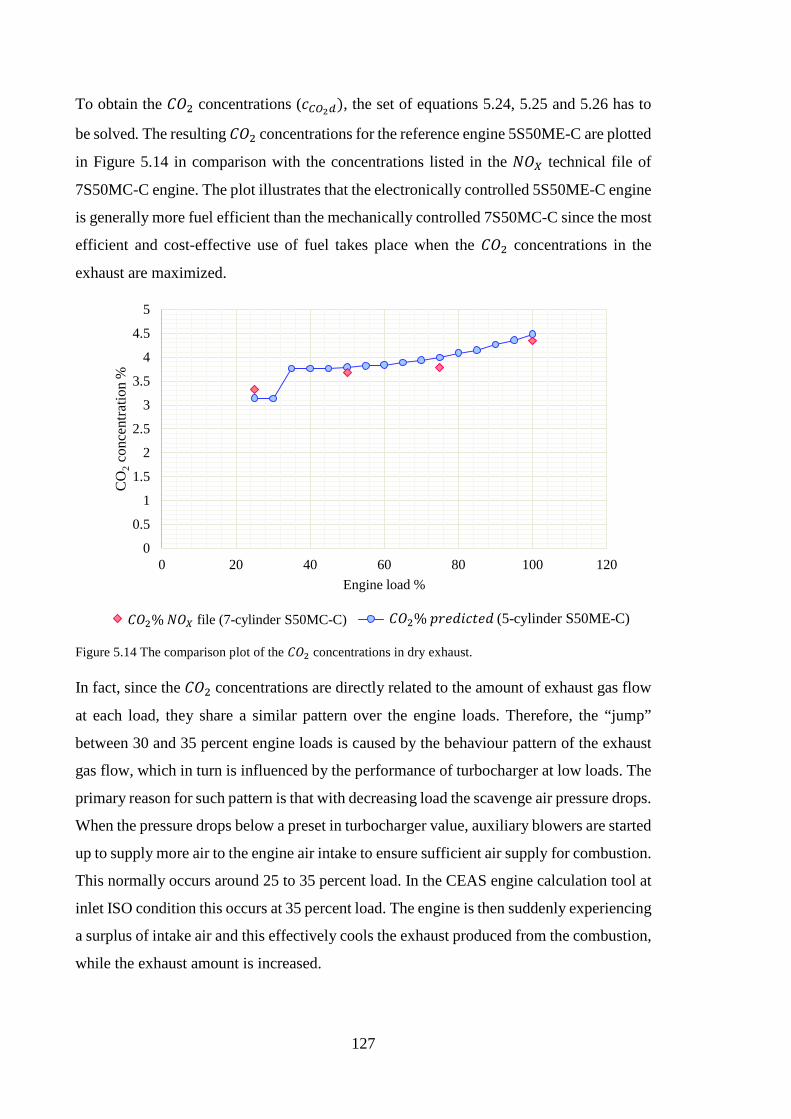
127
To obtain the 𝐶𝐶𝐶𝐶2 concentrations (𝐶𝐶𝐶𝐶𝑂𝑂2𝐴𝐴), the set of equations 5.24, 5.25 and 5.26 has to
be solved. The resulting 𝐶𝐶𝐶𝐶2 concentrations for the reference engine 5S50ME-C are plotted
in Figure 5.14 in comparison with the concentrations listed in the 𝑁𝑁𝐶𝐶𝑋𝑋 technical file of
7S50MC-C engine. The plot illustrates that the electronically controlled 5S50ME-C engine
is generally more fuel efficient than the mechanically controlled 7S50MC-C since the most
efficient and cost-effective use of fuel takes place when the 𝐶𝐶𝐶𝐶2 concentrations in the
exhaust are maximized.
Figure 5.14 The comparison plot of the 𝐶𝐶𝐶𝐶2 concentrations in dry exhaust.
In fact, since the 𝐶𝐶𝐶𝐶2 concentrations are directly related to the amount of exhaust gas flow
at each load, they share a similar pattern over the engine loads. Therefore, the “jump”
between 30 and 35 percent engine loads is caused by the behaviour pattern of the exhaust
gas flow, which in turn is influenced by the performance of turbocharger at low loads. The
primary reason for such pattern is that with decreasing load the scavenge air pressure drops.
When the pressure drops below a preset in turbocharger value, auxiliary blowers are started
up to supply more air to the engine air intake to ensure sufficient air supply for combustion.
This normally occurs around 25 to 35 percent load. In the CEAS engine calculation tool at
inlet ISO condition this occurs at 35 percent load. The engine is then suddenly experiencing
a surplus of intake air and this effectively cools the exhaust produced from the combustion,
while the exhaust amount is increased.
0
0.5
1
1.5
2
2.5
3
3.5
4
4.5
5
0 20 40 60 80 100 120
CO
2co
ncen
tratio
n %
Engine load %
𝐶𝐶𝐶𝐶2% 𝑁𝑁𝐶𝐶𝑋𝑋 file (7-cylinder S50MC-C) 𝐶𝐶𝐶𝐶2% 𝐶𝐶𝑡𝑡𝑒𝑒𝑑𝑑𝑖𝑖𝐶𝐶𝐶𝐶𝑒𝑒𝑑𝑑 (5-cylinder S50ME-C)
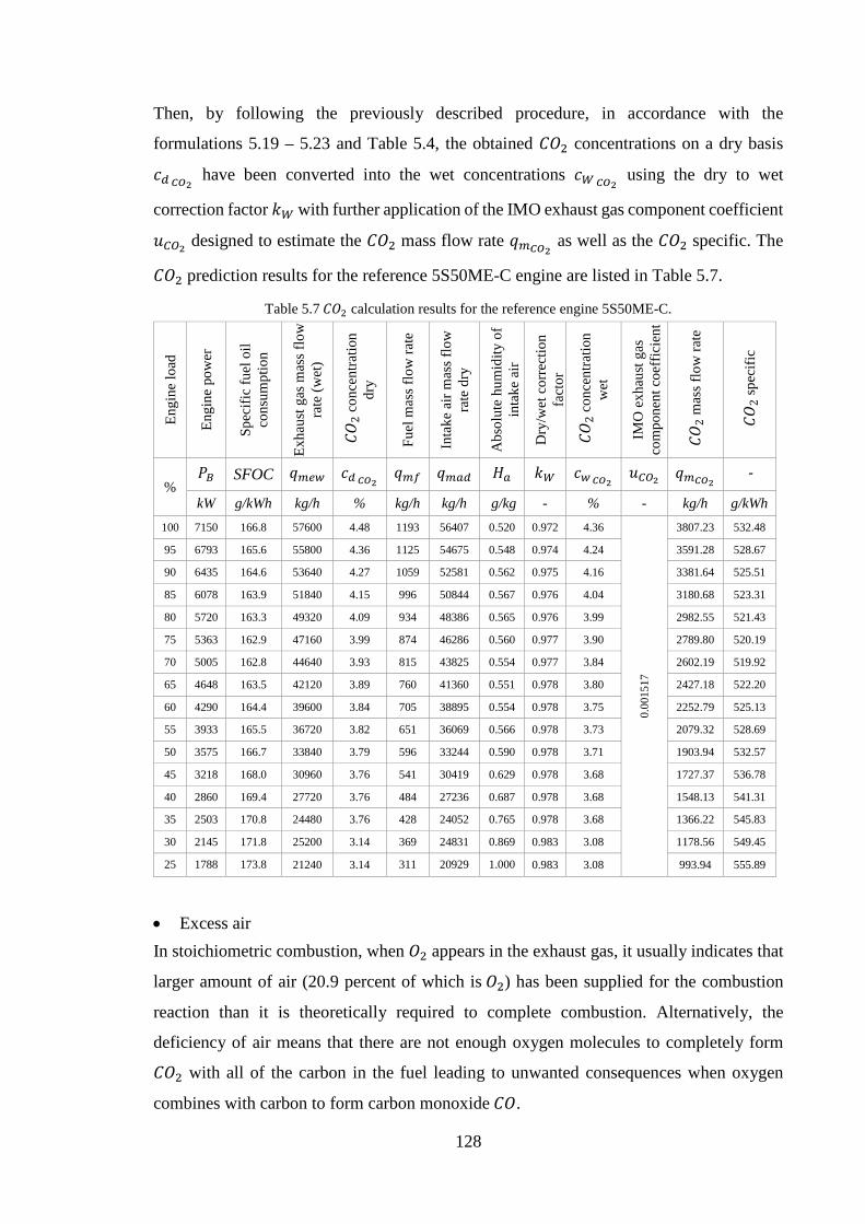
128
Then, by following the previously described procedure, in accordance with the
formulations 5.19 – 5.23 and Table 5.4, the obtained 𝐶𝐶𝐶𝐶2 concentrations on a dry basis
𝐶𝐶𝐴𝐴 𝐶𝐶𝐶𝐶2 have been converted into the wet concentrations 𝐶𝐶𝑊𝑊 𝐶𝐶𝐶𝐶2
using the dry to wet
correction factor 𝑘𝑘𝑊𝑊 with further application of the IMO exhaust gas component coefficient
𝑢𝑢𝐶𝐶𝑂𝑂2 designed to estimate the 𝐶𝐶𝐶𝐶2 mass flow rate 𝑞𝑞𝑚𝑚𝐶𝐶𝐶𝐶2 as well as the 𝐶𝐶𝐶𝐶2 specific. The
𝐶𝐶𝐶𝐶2 prediction results for the reference 5S50ME-C engine are listed in Table 5.7.
Table 5.7 𝐶𝐶𝐶𝐶2 calculation results for the reference engine 5S50ME-C.
Engi
ne lo
ad
Engi
ne p
ower
Spec
ific
fuel
oil
cons
umpt
ion
Exha
ust g
as m
ass f
low
ra
te (w
et)
𝐶𝐶𝐶𝐶
2 co
ncen
tratio
n dr
y
Fuel
mas
s flo
w ra
te
Inta
ke a
ir m
ass f
low
ra
te d
ry
Abs
olut
e hu
mid
ity o
f in
take
air
Dry
/wet
cor
rect
ion
fact
or
𝐶𝐶𝐶𝐶
2 co
ncen
tratio
n w
et
IMO
exh
aust
gas
co
mpo
nent
coe
ffic
ient
𝐶𝐶𝐶𝐶
2 m
ass f
low
rate
𝐶𝐶𝐶𝐶
2 sp
ecifi
c
% 𝑃𝑃𝐵𝐵 SFOC 𝑞𝑞𝑚𝑚𝐴𝐴𝑤𝑤 𝐶𝐶𝐴𝐴 𝐶𝐶𝐶𝐶2
𝑞𝑞𝑚𝑚𝑟𝑟 𝑞𝑞𝑚𝑚𝑔𝑔𝐴𝐴 𝐻𝐻𝑔𝑔 𝑘𝑘𝑊𝑊 𝐶𝐶𝑤𝑤 𝐶𝐶𝐶𝐶2 𝑢𝑢𝐶𝐶𝑂𝑂2 𝑞𝑞𝑚𝑚𝐶𝐶𝐶𝐶2
‐
kW g/kWh kg/h % kg/h kg/h g/kg - % - kg/h g/kWh 100 7150 166.8 57600 4.48 1193 56407 0.520 0.972 4.36
0.00
1517
3807.23 532.48
95 6793 165.6 55800 4.36 1125 54675 0.548 0.974 4.24 3591.28 528.67
90 6435 164.6 53640 4.27 1059 52581 0.562 0.975 4.16 3381.64 525.51
85 6078 163.9 51840 4.15 996 50844 0.567 0.976 4.04 3180.68 523.31
80 5720 163.3 49320 4.09 934 48386 0.565 0.976 3.99 2982.55 521.43
75 5363 162.9 47160 3.99 874 46286 0.560 0.977 3.90 2789.80 520.19
70 5005 162.8 44640 3.93 815 43825 0.554 0.977 3.84 2602.19 519.92
65 4648 163.5 42120 3.89 760 41360 0.551 0.978 3.80 2427.18 522.20
60 4290 164.4 39600 3.84 705 38895 0.554 0.978 3.75 2252.79 525.13
55 3933 165.5 36720 3.82 651 36069 0.566 0.978 3.73 2079.32 528.69
50 3575 166.7 33840 3.79 596 33244 0.590 0.978 3.71 1903.94 532.57
45 3218 168.0 30960 3.76 541 30419 0.629 0.978 3.68 1727.37 536.78
40 2860 169.4 27720 3.76 484 27236 0.687 0.978 3.68 1548.13 541.31
35 2503 170.8 24480 3.76 428 24052 0.765 0.978 3.68 1366.22 545.83
30 2145 171.8 25200 3.14 369 24831 0.869 0.983 3.08 1178.56 549.45
25 1788 173.8 21240 3.14 311 20929 1.000 0.983 3.08 993.94 555.89
• Excess air In stoichiometric combustion, when 𝐶𝐶2 appears in the exhaust gas, it usually indicates that
larger amount of air (20.9 percent of which is 𝐶𝐶2) has been supplied for the combustion
reaction than it is theoretically required to complete combustion. Alternatively, the
deficiency of air means that there are not enough oxygen molecules to completely form
𝐶𝐶𝐶𝐶2 with all of the carbon in the fuel leading to unwanted consequences when oxygen
combines with carbon to form carbon monoxide 𝐶𝐶𝐶𝐶.
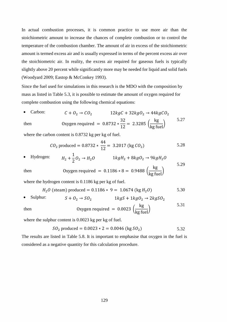
129
In actual combustion processes, it is common practice to use more air than the
stoichiometric amount to increase the chances of complete combustion or to control the
temperature of the combustion chamber. The amount of air in excess of the stoichiometric
amount is termed excess air and is usually expressed in terms of the percent excess air over
the stoichiometric air. In reality, the excess air required for gaseous fuels is typically
slightly above 20 percent while significantly more may be needed for liquid and solid fuels
(Woodyard 2009; Eastop & McConkey 1993).
Since the fuel used for simulations in this research is the MDO with the composition by
mass as listed in Table 5.3, it is possible to estimate the amount of oxygen required for
complete combustion using the following chemical equations:
• Carbon: 𝐶𝐶 + 𝐶𝐶2 → 𝐶𝐶𝐶𝐶2 12𝑘𝑘𝑔𝑔𝐶𝐶 + 32𝑘𝑘𝑔𝑔𝐶𝐶2 → 44𝑘𝑘𝑔𝑔𝐶𝐶𝐶𝐶2 5.27
then Oxygen required = 0.8732 ∗3212
= 2.3285 kg
kg fuel
where the carbon content is 0.8732 kg per kg of fuel.
𝐶𝐶𝐶𝐶2 produced = 0.8732 ∗ 4412
= 3.2017 (kg 𝐶𝐶𝐶𝐶2) 5.28
• Hydrogen: 𝐻𝐻2 +12𝐶𝐶2 → 𝐻𝐻2𝐶𝐶 1𝑘𝑘𝑔𝑔𝐻𝐻2 + 8𝑘𝑘𝑔𝑔𝐶𝐶2 → 9𝑘𝑘𝑔𝑔𝐻𝐻2𝐶𝐶
5.29 then Oxygen required = 0.1186 ∗ 8 = 0.9488
kgkg fuel
where the hydrogen content is 0.1186 kg per kg of fuel.
𝐻𝐻2𝐶𝐶 (steam) produced = 0.1186 ∗ 9 = 1.0674 (kg 𝐻𝐻2𝐶𝐶) 5.30 • Sulphur: 𝑆𝑆 + 𝐶𝐶2 → 𝑆𝑆𝐶𝐶2 1𝑘𝑘𝑔𝑔𝑆𝑆 + 1𝑘𝑘𝑔𝑔𝐶𝐶2 → 2𝑘𝑘𝑔𝑔𝑆𝑆𝐶𝐶2
5.31 then Oxygen required = 0.0023
kgkg fuel
where the sulphur content is 0.0023 kg per kg of fuel.
𝑆𝑆𝐶𝐶2 produced = 0.0023 ∗ 2 = 0.0046 (kg 𝑆𝑆𝐶𝐶2) 5.32
The results are listed in Table 5.8. It is important to emphasise that oxygen in the fuel is
considered as a negative quantity for this calculation procedure.
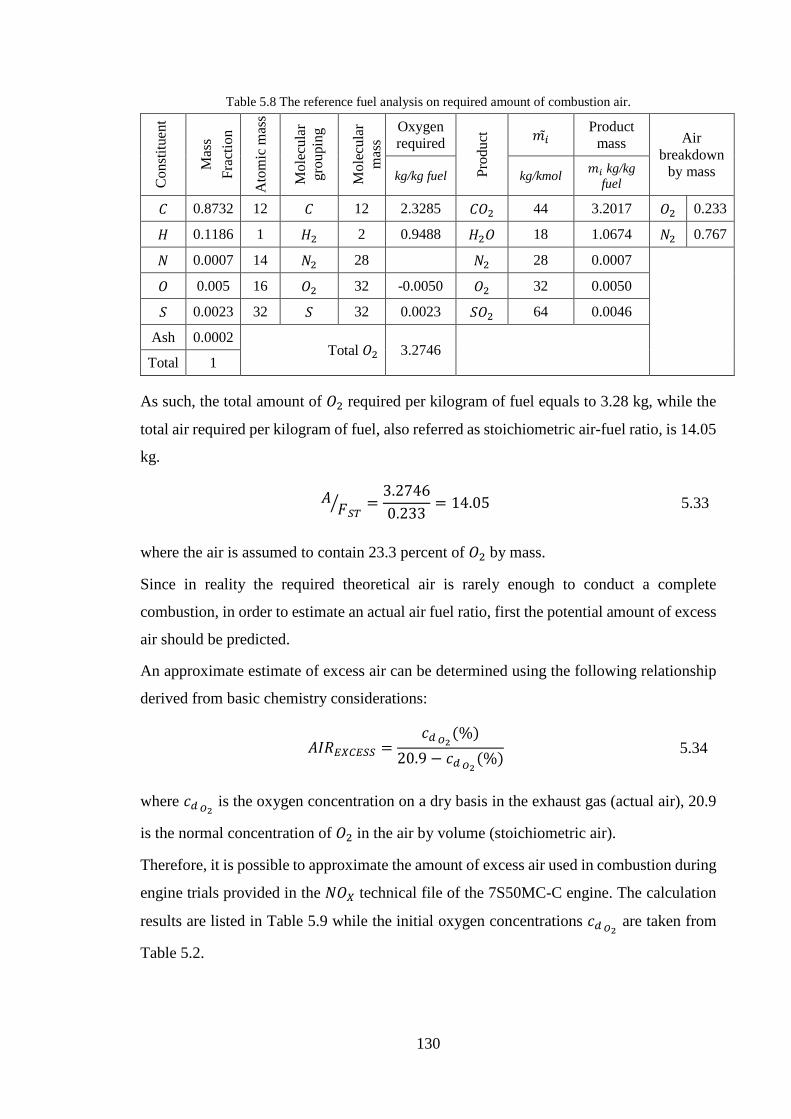
130
Table 5.8 The reference fuel analysis on required amount of combustion air.
Con
stitu
ent
M
ass
Frac
tion
A
tom
ic m
ass
M
olec
ular
gr
oupi
ng
M
olec
ular
m
ass
Oxygen required
Prod
uct 𝑛𝑛𝑚𝐴𝐴
Product mass Air
breakdown by mass kg/kg fuel kg/kmol 𝑛𝑛𝐴𝐴 kg/kg
fuel
𝐶𝐶 0.8732 12 𝐶𝐶 12 2.3285 𝐶𝐶𝐶𝐶2 44 3.2017 𝐶𝐶2 0.233
𝐻𝐻 0.1186 1 𝐻𝐻2 2 0.9488 𝐻𝐻2𝐶𝐶 18 1.0674 𝑁𝑁2 0.767
𝑁𝑁 0.0007 14 𝑁𝑁2 28 𝑁𝑁2 28 0.0007
𝐶𝐶 0.005 16 𝐶𝐶2 32 -0.0050 𝐶𝐶2 32 0.0050
𝑆𝑆 0.0023 32 𝑆𝑆 32 0.0023 𝑆𝑆𝐶𝐶2 64 0.0046
Ash 0.0002 Total 𝐶𝐶2 3.2746
Total 1
As such, the total amount of 𝐶𝐶2 required per kilogram of fuel equals to 3.28 kg, while the
total air required per kilogram of fuel, also referred as stoichiometric air-fuel ratio, is 14.05
kg.
𝐵𝐵𝑆𝑆 𝑆𝑆𝑇𝑇
=3.27460.233
= 14.05 5.33
where the air is assumed to contain 23.3 percent of 𝐶𝐶2 by mass.
Since in reality the required theoretical air is rarely enough to conduct a complete
combustion, in order to estimate an actual air fuel ratio, first the potential amount of excess
air should be predicted.
An approximate estimate of excess air can be determined using the following relationship
derived from basic chemistry considerations:
𝐵𝐵𝐸𝐸𝐵𝐵𝐸𝐸𝑋𝑋𝐶𝐶𝐸𝐸𝑆𝑆𝑆𝑆 =𝐶𝐶𝐴𝐴 𝐶𝐶2
(%)20.9 − 𝐶𝐶𝐴𝐴 𝐶𝐶2
(%) 5.34
where 𝐶𝐶𝐴𝐴 𝐶𝐶2 is the oxygen concentration on a dry basis in the exhaust gas (actual air), 20.9
is the normal concentration of 𝐶𝐶2 in the air by volume (stoichiometric air).
Therefore, it is possible to approximate the amount of excess air used in combustion during
engine trials provided in the 𝑁𝑁𝐶𝐶𝑋𝑋 technical file of the 7S50MC-C engine. The calculation
results are listed in Table 5.9 while the initial oxygen concentrations 𝐶𝐶𝐴𝐴 𝐶𝐶2 are taken from
Table 5.2.

131
Table 5.9 The excess air approximation results for 7S50MC-C engine.
Engine load 𝐶𝐶2 Excess air ratio % %
100 15.23 2.69
75 15.95 3.22
50 16.15 3.4
25 16.58 3.84
Based on predicted excess air supply for each load, the actual air-fuel ratios estimated using
the following procedure:
𝐵𝐵𝑆𝑆 𝐴𝐴𝐶𝐶𝑇𝑇
= 𝐵𝐵𝑆𝑆 𝑆𝑆𝑇𝑇
+ 𝐵𝐵𝑆𝑆 𝑆𝑆𝑇𝑇
∗ 𝐵𝐵𝐸𝐸𝐵𝐵𝐸𝐸𝑋𝑋𝐶𝐶𝐸𝐸𝑆𝑆𝑆𝑆 5.35
where 𝐵𝐵 𝑆𝑆 𝑆𝑆𝑇𝑇 is the stoichiometric air-fuel ratio and 𝐵𝐵𝐸𝐸𝐵𝐵𝐸𝐸𝑋𝑋𝐶𝐶𝐸𝐸𝑆𝑆𝑆𝑆 is the excess air ratio
estimated for each load.
Thus, it is possible to calculate the amount of 𝑁𝑁2 and 𝐶𝐶2 products supplied by mass for
combustion with the influence of excess air as well as to find the overall mass of products
at each engine load using the following relationships based on the basic chemistry
considerations:
Nitrogen: 𝑛𝑛𝑆𝑆2𝐴𝐴𝐴𝐴𝑅𝑅= 0.767 𝐵𝐵 𝑆𝑆 𝐴𝐴𝐶𝐶𝑇𝑇
+ 𝑛𝑛𝑆𝑆2 5.36
Oxygen: 𝑛𝑛𝑂𝑂2𝐴𝐴𝐴𝐴𝑅𝑅= 0.233 𝐵𝐵 𝑆𝑆 𝐴𝐴𝐶𝐶𝑇𝑇
− 𝐶𝐶2𝑇𝑇𝑂𝑂𝑇𝑇𝐴𝐴𝑊𝑊 5.37
Total mass: 𝑛𝑛𝑇𝑇𝑂𝑂𝑇𝑇𝐴𝐴𝑊𝑊 = 𝑛𝑛𝐶𝐶𝑂𝑂2 + 𝑛𝑛𝐻𝐻2𝑂𝑂 + 𝑛𝑛𝑆𝑆2𝐸𝐸𝑋𝑋𝐶𝐶 𝐴𝐴𝐴𝐴𝑅𝑅+ 𝑛𝑛𝑂𝑂2𝐸𝐸𝑋𝑋𝐶𝐶 𝐴𝐴𝐴𝐴𝑅𝑅
+ 𝑛𝑛𝑆𝑆𝑂𝑂2 5.38
where
- 𝑛𝑛𝑆𝑆2 is the mass of exhaust nitrogen without the influence of excess air;
- 𝐶𝐶2𝑇𝑇𝑂𝑂𝑇𝑇𝐴𝐴𝑊𝑊 is the total amount of 𝐶𝐶2 required per kilogram of fuel;
- 𝑛𝑛𝑆𝑆2𝐴𝐴𝐴𝐴𝑅𝑅and 𝑛𝑛𝑂𝑂2 𝐴𝐴𝐴𝐴𝑅𝑅
are the amounts of nitrogen and oxygen with respect to the
excess air obtained for each load;
- 𝑛𝑛𝐶𝐶𝑂𝑂2, 𝑛𝑛𝐻𝐻2𝑂𝑂, 𝑛𝑛𝑆𝑆𝑂𝑂2 are the product masses of carbon dioxide, steam and sulphur
dioxide per kg of fuel respectively.
The results of this calculation procedure based on the 𝑁𝑁𝐶𝐶𝑋𝑋 technical file data of the
7S50MC-C engine are tabulated in Table 5.10.
In Table 5.11 the amount of substance (𝑛𝑛) in kmol per kilogram of fuel is given by equation
(5.39).
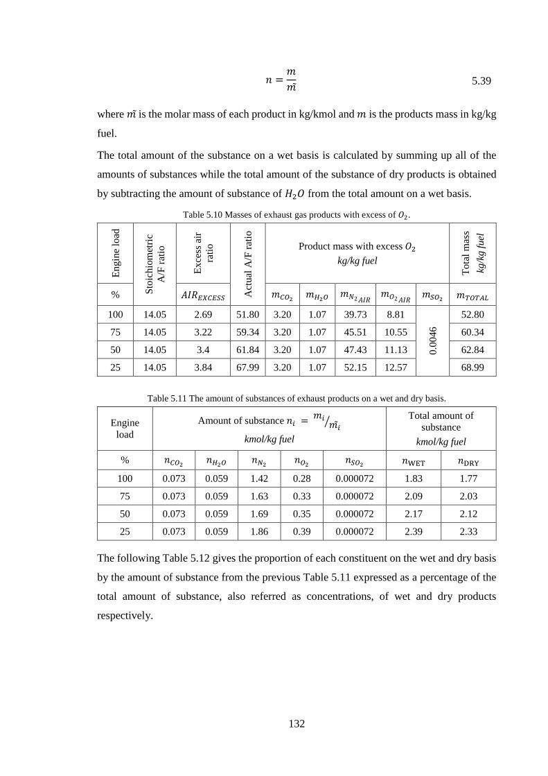
132
𝑛𝑛 =𝑛𝑛𝑛𝑛𝑚
5.39
where 𝑛𝑛𝑚 is the molar mass of each product in kg/kmol and 𝑛𝑛 is the products mass in kg/kg
fuel.
The total amount of the substance on a wet basis is calculated by summing up all of the
amounts of substances while the total amount of the substance of dry products is obtained
by subtracting the amount of substance of 𝐻𝐻2𝐶𝐶 from the total amount on a wet basis.
Table 5.10 Masses of exhaust gas products with excess of 𝐶𝐶2.
Engi
ne lo
ad
Stoi
chio
met
ric
A/F
ratio
Exce
ss a
ir ra
tio
Act
ual A
/F ra
tio
Product mass with excess 𝐶𝐶2 kg/kg fuel
Tota
l mas
s kg
/kg
fuel
% 𝐵𝐵𝐸𝐸𝐵𝐵𝐸𝐸𝑋𝑋𝐶𝐶𝐸𝐸𝑆𝑆𝑆𝑆 𝑛𝑛𝐶𝐶𝑂𝑂2 𝑛𝑛𝐻𝐻2𝑂𝑂 𝑛𝑛𝑁𝑁2𝐵𝐵𝐸𝐸𝐵𝐵 𝑛𝑛𝐶𝐶2𝐵𝐵𝐸𝐸𝐵𝐵
𝑛𝑛𝑆𝑆𝑂𝑂2 𝑛𝑛𝑇𝑇𝑂𝑂𝑇𝑇𝐴𝐴𝑊𝑊
100 14.05 2.69 51.80 3.20 1.07 39.73 8.81
0.00
46
52.80
75 14.05 3.22 59.34 3.20 1.07 45.51 10.55 60.34
50 14.05 3.4 61.84 3.20 1.07 47.43 11.13 62.84
25 14.05 3.84 67.99 3.20 1.07 52.15 12.57 68.99
Table 5.11 The amount of substances of exhaust products on a wet and dry basis.
Engine load
Amount of substance 𝑛𝑛𝐴𝐴 = 𝑛𝑛𝐴𝐴𝑛𝑛𝑚𝐴𝐴
kmol/kg fuel
Total amount of substance
kmol/kg fuel
% 𝑛𝑛𝐶𝐶𝑂𝑂2 𝑛𝑛𝐻𝐻2𝑂𝑂 𝑛𝑛𝑆𝑆2 𝑛𝑛𝑂𝑂2 𝑛𝑛𝑆𝑆𝑂𝑂2 𝑛𝑛WET 𝑛𝑛DRY
100 0.073 0.059 1.42 0.28 0.000072 1.83 1.77
75 0.073 0.059 1.63 0.33 0.000072 2.09 2.03
50 0.073 0.059 1.69 0.35 0.000072 2.17 2.12
25 0.073 0.059 1.86 0.39 0.000072 2.39 2.33
The following Table 5.12 gives the proportion of each constituent on the wet and dry basis
by the amount of substance from the previous Table 5.11 expressed as a percentage of the
total amount of substance, also referred as concentrations, of wet and dry products
respectively.
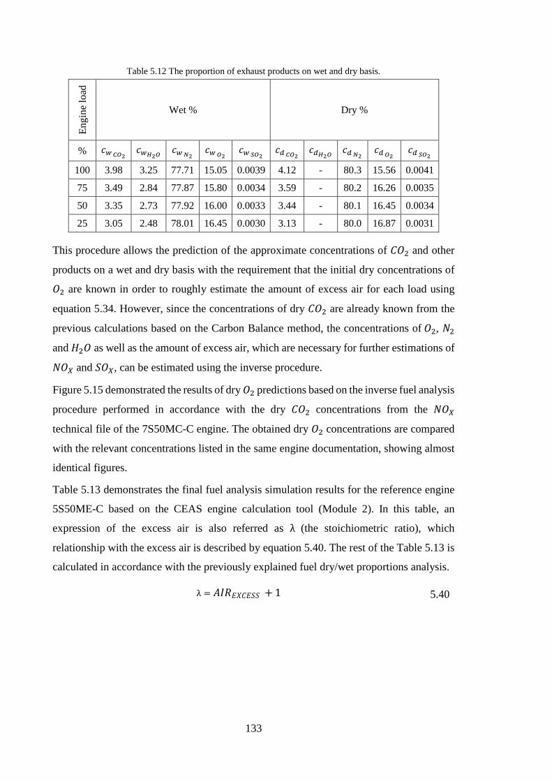
133
Table 5.12 The proportion of exhaust products on wet and dry basis. En
gine
load
Wet % Dry %
% 𝐶𝐶𝑤𝑤 𝐶𝐶𝐶𝐶2 𝐶𝐶𝑤𝑤𝐻𝐻2𝐶𝐶
𝐶𝐶𝑤𝑤 𝑁𝑁2 𝐶𝐶𝑤𝑤 𝐶𝐶2
𝐶𝐶𝑤𝑤 𝑆𝑆𝐶𝐶2 𝐶𝐶𝐴𝐴 𝐶𝐶𝐶𝐶2
𝐶𝐶𝐴𝐴𝐻𝐻2𝐶𝐶 𝐶𝐶𝐴𝐴 𝑁𝑁2 𝐶𝐶𝐴𝐴 𝐶𝐶2
𝐶𝐶𝐴𝐴 𝑆𝑆𝐶𝐶2
100 3.98 3.25 77.71 15.05 0.0039 4.12 - 80.3 15.56 0.0041
75 3.49 2.84 77.87 15.80 0.0034 3.59 - 80.2 16.26 0.0035
50 3.35 2.73 77.92 16.00 0.0033 3.44 - 80.1 16.45 0.0034
25 3.05 2.48 78.01 16.45 0.0030 3.13 - 80.0 16.87 0.0031
This procedure allows the prediction of the approximate concentrations of 𝐶𝐶𝐶𝐶2 and other
products on a wet and dry basis with the requirement that the initial dry concentrations of
𝐶𝐶2 are known in order to roughly estimate the amount of excess air for each load using
equation 5.34. However, since the concentrations of dry 𝐶𝐶𝐶𝐶2 are already known from the
previous calculations based on the Carbon Balance method, the concentrations of 𝐶𝐶2, 𝑁𝑁2
and 𝐻𝐻2𝐶𝐶 as well as the amount of excess air, which are necessary for further estimations of
𝑁𝑁𝐶𝐶𝑋𝑋 and 𝑆𝑆𝐶𝐶𝑋𝑋, can be estimated using the inverse procedure.
Figure 5.15 demonstrated the results of dry 𝐶𝐶2 predictions based on the inverse fuel analysis
procedure performed in accordance with the dry 𝐶𝐶𝐶𝐶2 concentrations from the 𝑁𝑁𝐶𝐶𝑋𝑋
technical file of the 7S50MC-C engine. The obtained dry 𝐶𝐶2 concentrations are compared
with the relevant concentrations listed in the same engine documentation, showing almost
identical figures.
Table 5.13 demonstrates the final fuel analysis simulation results for the reference engine
5S50ME-C based on the CEAS engine calculation tool (Module 2). In this table, an
expression of the excess air is also referred as λ (the stoichiometric ratio), which
relationship with the excess air is described by equation 5.40. The rest of the Table 5.13 is
calculated in accordance with the previously explained fuel dry/wet proportions analysis.
λ = 𝐵𝐵𝐸𝐸𝐵𝐵𝐸𝐸𝑋𝑋𝐶𝐶𝐸𝐸𝑆𝑆𝑆𝑆 + 1 5.40
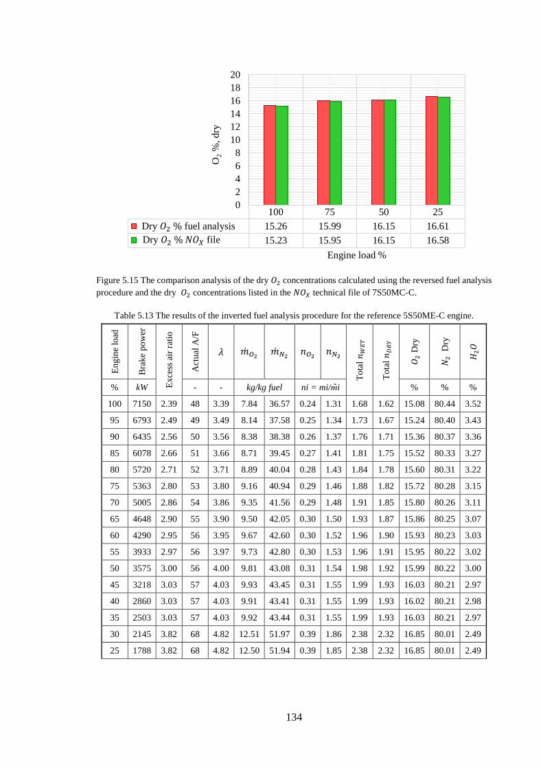
134
Figure 5.15 The comparison analysis of the dry 𝐶𝐶2 concentrations calculated using the reversed fuel analysis procedure and the dry 𝐶𝐶2 concentrations listed in the 𝑁𝑁𝐶𝐶𝑋𝑋 technical file of 7S50MC-C.
Table 5.13 The results of the inverted fuel analysis procedure for the reference 5S50ME-C engine.
Engi
ne lo
ad
Bra
ke p
ower
Exce
ss a
ir ra
tio
Act
ual A
/F
𝜆𝜆 𝑛𝑂𝑂2 𝑛𝑆𝑆2 𝑛𝑛𝑂𝑂2 𝑛𝑛𝑆𝑆2 To
tal 𝑛𝑛
𝑊𝑊𝐸𝐸𝑇𝑇
Tota
l 𝑛𝑛𝐷𝐷𝑅𝑅𝐷𝐷
𝐶𝐶 2
Dry
𝑁𝑁 2 D
ry
𝐻𝐻 2𝐶𝐶
% kW - - kg/kg fuel ni = mi/mi % % %
100 7150 2.39 48 3.39 7.84 36.57 0.24 1.31 1.68 1.62 15.08 80.44 3.52
95 6793 2.49 49 3.49 8.14 37.58 0.25 1.34 1.73 1.67 15.24 80.40 3.43
90 6435 2.56 50 3.56 8.38 38.38 0.26 1.37 1.76 1.71 15.36 80.37 3.36
85 6078 2.66 51 3.66 8.71 39.45 0.27 1.41 1.81 1.75 15.52 80.33 3.27
80 5720 2.71 52 3.71 8.89 40.04 0.28 1.43 1.84 1.78 15.60 80.31 3.22
75 5363 2.80 53 3.80 9.16 40.94 0.29 1.46 1.88 1.82 15.72 80.28 3.15
70 5005 2.86 54 3.86 9.35 41.56 0.29 1.48 1.91 1.85 15.80 80.26 3.11
65 4648 2.90 55 3.90 9.50 42.05 0.30 1.50 1.93 1.87 15.86 80.25 3.07
60 4290 2.95 56 3.95 9.67 42.60 0.30 1.52 1.96 1.90 15.93 80.23 3.03
55 3933 2.97 56 3.97 9.73 42.80 0.30 1.53 1.96 1.91 15.95 80.22 3.02
50 3575 3.00 56 4.00 9.81 43.08 0.31 1.54 1.98 1.92 15.99 80.22 3.00
45 3218 3.03 57 4.03 9.93 43.45 0.31 1.55 1.99 1.93 16.03 80.21 2.97
40 2860 3.03 57 4.03 9.91 43.41 0.31 1.55 1.99 1.93 16.02 80.21 2.98
35 2503 3.03 57 4.03 9.92 43.44 0.31 1.55 1.99 1.93 16.03 80.21 2.97
30 2145 3.82 68 4.82 12.51 51.97 0.39 1.86 2.38 2.32 16.85 80.01 2.49
25 1788 3.82 68 4.82 12.50 51.94 0.39 1.85 2.38 2.32 16.85 80.01 2.49
100 75 50 2515.26 15.99 16.15 16.6115.23 15.95 16.15 16.58
02468
101214161820
O2
%, d
ry
Engine load %
Dry 𝐶𝐶2 % fuel analysisDry 𝐶𝐶2 % 𝑁𝑁𝐶𝐶𝑋𝑋 file

135
• Nitrogen oxides (𝑁𝑁𝐶𝐶𝑋𝑋) While nitric oxide (𝑁𝑁𝐶𝐶) and nitric dioxide (𝑁𝑁𝐶𝐶2) are normally grouped together as
𝑁𝑁𝐶𝐶𝑋𝑋 emissions, nitric oxide (𝑁𝑁𝐶𝐶) is the predominant nitrogen component formed inside
the engine cylinder. The principal source of 𝑁𝑁𝐶𝐶 is the oxidation of atmospheric nitrogen at
high temperatures (Heywood 1985). However, if the fuel contains a significant amount of
nitrogen, its oxidation becomes an additional source of 𝑁𝑁𝐶𝐶, which is particularly common
for diesel fuels.
In a number of publications, including (Heywood 1985; Flagan & Seinfeld 1988; Flynn
2003), a general principle of thermal 𝑁𝑁𝐶𝐶 formation is described by the ‘extended
Zeldovich’ mechanism influenced by a local combustion environment. This approach has
been successfully verified by experimental analysis and considered to be an effective
method for 𝑁𝑁𝐶𝐶𝑋𝑋 prediction. For instance, a multi-zone combustion diagnostic model
developed by (Egnell 1998), is able to estimate 𝑁𝑁𝐶𝐶 at the combustion zone and post-
combustion zones separately by means of the Zeldovich mechanism based on the measured
pressure data, which is necessary to calculate the local temperatures, and the arbitrarily
chosen stoichiometric ratio 𝜆𝜆 in each zone.
In general, the combustion diagnostic approaches could be very precise in predicting 𝑁𝑁𝐶𝐶𝑋𝑋
emissions and other species, mainly due to a detailed simulation of the thermodynamic
processes. However, since the cylinder space is divided into a number of zones, while each
zone has to solve a set of differential equations, the overall model algorithm is complicated
and requires extensive initial data and considered to be very time-consuming.
In addition, a number of computational methods are available to approximate 𝑁𝑁𝐶𝐶𝑋𝑋
concentrations in the exhaust gas. The choice of the right method is, to a large extent,
influenced by the availability of the required data to perform a simulation. For instance,
black box simulation models, based on advanced non-linear approximations using
mathematical algorithms, or artificial neural networks require an extensive engine
performance dataset or direct measurements. A neural network based 𝑁𝑁𝐶𝐶𝑋𝑋 prediction
models outlined in (Kristensen 2012) require real-time inputs of the inlet pressure, the inlet
temperature, the engine speed as well as the fuel rack position supported by several initial
data points in order to successfully train the model.
Alternatively, the analytical approaches based on polynomial regression analysis can be
used for 𝑁𝑁𝐶𝐶𝑋𝑋 prediction purposes and the accuracy level of such methods can be high. For
instance, in (Murphy et al. 2013), a multi linear regression method is used to develop a
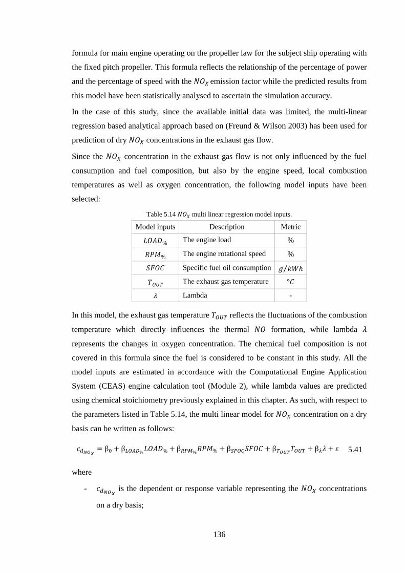
136
formula for main engine operating on the propeller law for the subject ship operating with
the fixed pitch propeller. This formula reflects the relationship of the percentage of power
and the percentage of speed with the 𝑁𝑁𝐶𝐶𝑋𝑋 emission factor while the predicted results from
this model have been statistically analysed to ascertain the simulation accuracy.
In the case of this study, since the available initial data was limited, the multi-linear
regression based analytical approach based on (Freund & Wilson 2003) has been used for
prediction of dry 𝑁𝑁𝐶𝐶𝑋𝑋 concentrations in the exhaust gas flow.
Since the 𝑁𝑁𝐶𝐶𝑋𝑋 concentration in the exhaust gas flow is not only influenced by the fuel
consumption and fuel composition, but also by the engine speed, local combustion
temperatures as well as oxygen concentration, the following model inputs have been
selected:
Table 5.14 𝑁𝑁𝐶𝐶𝑋𝑋 multi linear regression model inputs.
Model inputs Description Metric
𝐿𝐿𝐶𝐶𝐵𝐵𝐷𝐷% The engine load %
𝐵𝐵𝑃𝑃𝑁𝑁% The engine rotational speed %
𝑆𝑆𝑆𝑆𝐶𝐶𝐶𝐶 Specific fuel oil consumption 𝑔𝑔 𝑘𝑘𝑊𝑊ℎ⁄
𝑃𝑃𝐶𝐶𝑂𝑂𝑃𝑃 The exhaust gas temperature °𝐶𝐶
𝜆𝜆 Lambda -
In this model, the exhaust gas temperature 𝑃𝑃𝑂𝑂𝑂𝑂𝑇𝑇 reflects the fluctuations of the combustion
temperature which directly influences the thermal 𝑁𝑁𝐶𝐶 formation, while lambda 𝜆𝜆
represents the changes in oxygen concentration. The chemical fuel composition is not
covered in this formula since the fuel is considered to be constant in this study. All the
model inputs are estimated in accordance with the Computational Engine Application
System (CEAS) engine calculation tool (Module 2), while lambda values are predicted
using chemical stoichiometry previously explained in this chapter. As such, with respect to
the parameters listed in Table 5.14, the multi linear model for 𝑁𝑁𝐶𝐶𝑋𝑋 concentration on a dry
basis can be written as follows:
𝐶𝐶𝐴𝐴𝑁𝑁𝐶𝐶𝑋𝑋 = β0 + β𝑊𝑊𝑂𝑂𝐴𝐴𝐷𝐷%𝐿𝐿𝐶𝐶𝐵𝐵𝐷𝐷% + β𝑅𝑅𝑃𝑃𝑀𝑀%𝐵𝐵𝑃𝑃𝑁𝑁% + β𝑆𝑆𝐹𝐹𝑂𝑂𝐶𝐶𝑆𝑆𝑆𝑆𝐶𝐶𝐶𝐶 + β𝑇𝑇𝐶𝐶𝑂𝑂𝑂𝑂𝑃𝑃𝑂𝑂𝑂𝑂𝑇𝑇 + β𝜆𝜆𝜆𝜆 + 𝜀𝜀 5.41
where
- 𝐶𝐶𝐴𝐴𝑁𝑁𝐶𝐶𝑋𝑋 is the dependent or response variable representing the 𝑁𝑁𝐶𝐶𝑋𝑋 concentrations
on a dry basis;
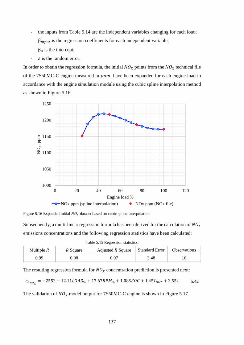
137
- the inputs from Table 5.14 are the independent variables changing for each load;
- β𝐴𝐴𝐴𝐴𝑖𝑖𝑅𝑅𝐴𝐴 is the regression coefficients for each independent variable;
- β0 is the intercept;
- 𝜀𝜀 is the random error.
In order to obtain the regression formula, the initial 𝑁𝑁𝐶𝐶𝑋𝑋 points from the 𝑁𝑁𝐶𝐶𝑋𝑋 technical file
of the 7S50MC-C engine measured in 𝐶𝐶𝐶𝐶𝑛𝑛, have been expanded for each engine load in
accordance with the engine simulation module using the cubic spline interpolation method
as shown in Figure 5.16.
Figure 5.16 Expanded initial 𝑁𝑁𝐶𝐶𝑋𝑋 dataset based on cubic spline interpolation.
Subsequently, a multi-linear regression formula has been derived for the calculation of 𝑁𝑁𝐶𝐶𝑋𝑋
emissions concentrations and the following regression statistics have been calculated:
Table 5.15 Regression statistics.
Multiple 𝐵𝐵 𝐵𝐵 Square Adjusted 𝐵𝐵 Square Standard Error Observations
0.99 0.98 0.97 3.48 16
The resulting regression formula for 𝑁𝑁𝐶𝐶𝑋𝑋 concentration prediction is presented next:
𝐶𝐶𝐴𝐴𝑁𝑁𝐶𝐶𝑋𝑋 = −2552 − 12.11𝐿𝐿𝐶𝐶𝐵𝐵𝐷𝐷% + 17.67𝐵𝐵𝑃𝑃𝑁𝑁% + 1.08𝑆𝑆𝑆𝑆𝐶𝐶𝐶𝐶 + 1.45𝑃𝑃𝑂𝑂𝑂𝑂𝑇𝑇 + 2.55𝜆𝜆 5.42
The validation of 𝑁𝑁𝐶𝐶𝑋𝑋 model output for 7S50MC-C engine is shown in Figure 5.17.
1000
1050
1100
1150
1200
1250
0 20 40 60 80 100 120
NO
X, p
pm
Engine load %NOx ppm (spline interpolation) NOx ppm (NOx file)
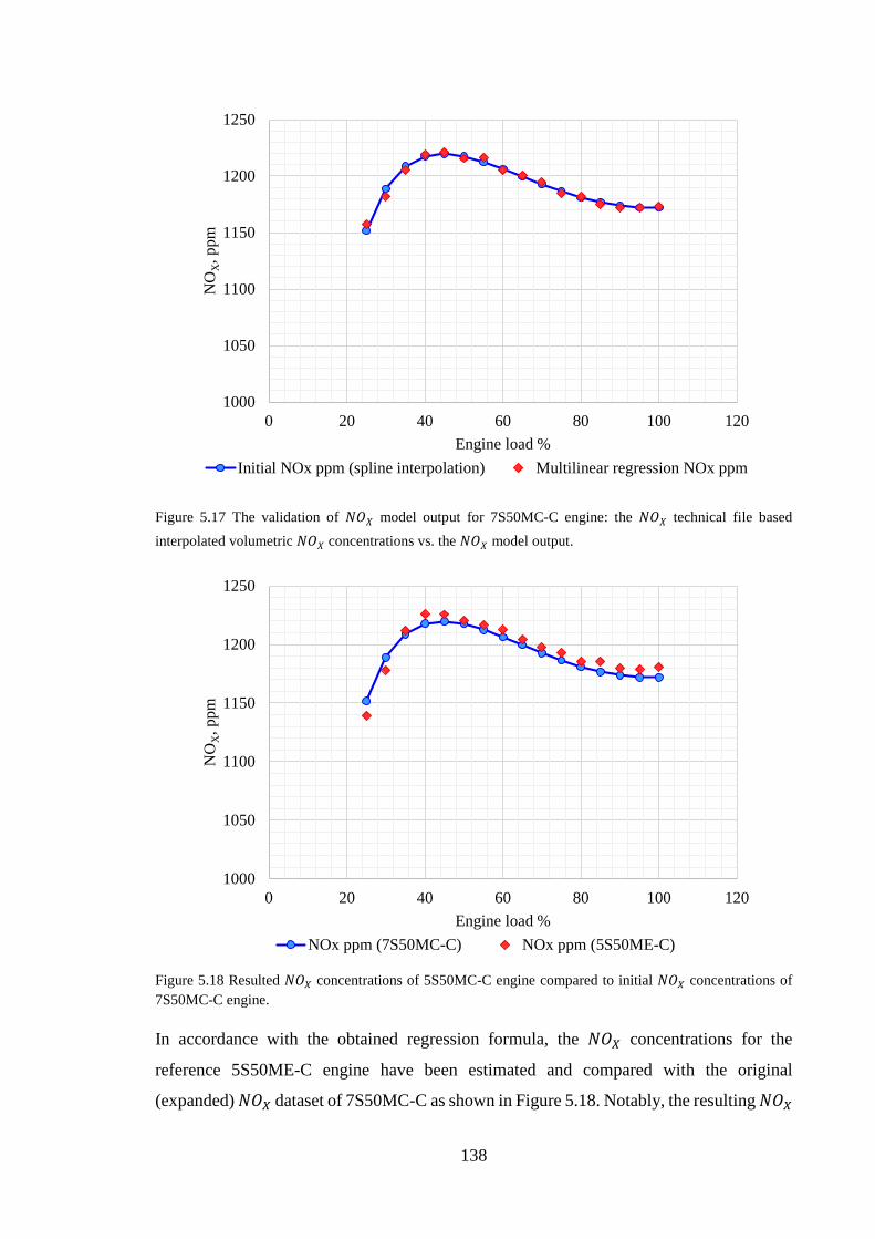
138
Figure 5.17 The validation of 𝑁𝑁𝐶𝐶𝑋𝑋 model output for 7S50MC-C engine: the 𝑁𝑁𝐶𝐶𝑋𝑋 technical file based interpolated volumetric 𝑁𝑁𝐶𝐶𝑋𝑋 concentrations vs. the 𝑁𝑁𝐶𝐶𝑋𝑋 model output.
Figure 5.18 Resulted 𝑁𝑁𝐶𝐶𝑋𝑋 concentrations of 5S50MC-C engine compared to initial 𝑁𝑁𝐶𝐶𝑋𝑋 concentrations of 7S50MC-C engine.
In accordance with the obtained regression formula, the 𝑁𝑁𝐶𝐶𝑋𝑋 concentrations for the
reference 5S50ME-C engine have been estimated and compared with the original
(expanded) 𝑁𝑁𝐶𝐶𝑋𝑋 dataset of 7S50MC-C as shown in Figure 5.18. Notably, the resulting 𝑁𝑁𝐶𝐶𝑋𝑋
1000
1050
1100
1150
1200
1250
0 20 40 60 80 100 120
NO
X, p
pm
Engine load %Initial NOx ppm (spline interpolation) Multilinear regression NOx ppm
1000
1050
1100
1150
1200
1250
0 20 40 60 80 100 120
NO
X, p
pm
Engine load %NOx ppm (7S50MC-C) NOx ppm (5S50ME-C)
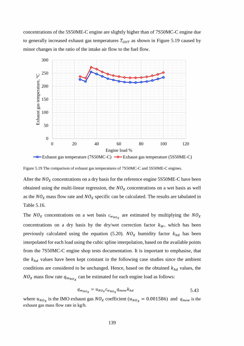
139
concentrations of the 5S50ME-C engine are slightly higher than of 7S50MC-C engine due
to generally increased exhaust gas temperatures 𝑃𝑃𝑂𝑂𝑂𝑂𝑇𝑇 as shown in Figure 5.19 caused by
minor changes in the ratio of the intake air flow to the fuel flow.
Figure 5.19 The comparison of exhaust gas temperatures of 7S50MC-C and 5S50ME-C engines.
After the 𝑁𝑁𝐶𝐶𝑋𝑋 concentrations on a dry basis for the reference engine 5S50ME-C have been
obtained using the multi-linear regression, the 𝑁𝑁𝐶𝐶𝑋𝑋 concentrations on a wet basis as well
as the 𝑁𝑁𝐶𝐶𝑋𝑋 mass flow rate and 𝑁𝑁𝐶𝐶𝑋𝑋 specific can be calculated. The results are tabulated in
Table 5.16.
The 𝑁𝑁𝐶𝐶𝑋𝑋 concentrations on a wet basis 𝐶𝐶𝑤𝑤𝑁𝑁𝐶𝐶𝑋𝑋 are estimated by multiplying the 𝑁𝑁𝐶𝐶𝑋𝑋
concentrations on a dry basis by the dry/wet correction factor 𝑘𝑘𝑊𝑊, which has been
previously calculated using the equation (5.20). 𝑁𝑁𝐶𝐶𝑋𝑋 humidity factor 𝑘𝑘ℎ𝐴𝐴 has been
interpolated for each load using the cubic spline interpolation, based on the available points
from the 7S50MC-C engine shop tests documentation. It is important to emphasise, that
the 𝑘𝑘ℎ𝐴𝐴 values have been kept constant in the following case studies since the ambient
conditions are considered to be unchanged. Hence, based on the obtained 𝑘𝑘ℎ𝐴𝐴 values, the
𝑁𝑁𝐶𝐶𝑋𝑋 mass flow rate 𝑞𝑞𝑚𝑚𝑁𝑁𝐶𝐶𝑋𝑋 can be estimated for each engine load as follows:
𝑞𝑞𝑚𝑚𝑁𝑁𝐶𝐶𝑋𝑋= 𝑢𝑢𝑆𝑆𝑂𝑂𝑋𝑋𝐶𝐶𝑤𝑤𝑁𝑁𝐶𝐶𝑋𝑋
𝑞𝑞𝑚𝑚𝐴𝐴𝑤𝑤𝑘𝑘ℎ𝐴𝐴 5.43
where 𝑢𝑢𝑆𝑆𝑂𝑂𝑋𝑋 is the IMO exhaust gas 𝑁𝑁𝐶𝐶𝑋𝑋 coefficient (𝑢𝑢𝑆𝑆𝑂𝑂𝑋𝑋 = 0.001586) and 𝑞𝑞𝑚𝑚𝐴𝐴𝑤𝑤 is the exhaust gas mass flow rate in kg/h.
0
50
100
150
200
250
300
0 20 40 60 80 100 120
Exha
ust g
as te
mpe
ratu
re, °
C
Engine load %Exhaust gas temperature (7S50MC-C) Exhaust gas temperature (5S50ME-C)
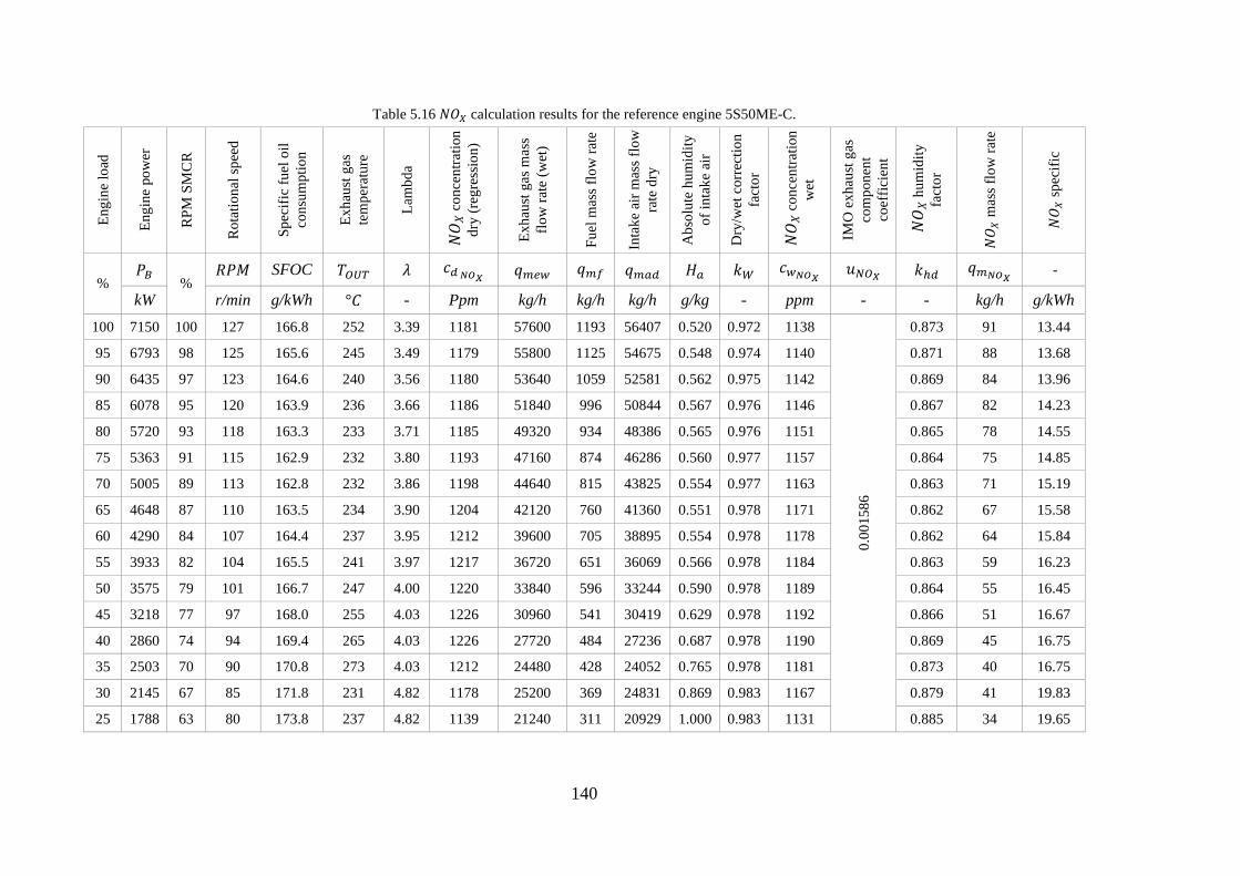
140
Table 5.16 𝑁𝑁𝐶𝐶𝑋𝑋 calculation results for the reference engine 5S50ME-C. En
gine
load
Engi
ne p
ower
RPM
SM
CR
Rot
atio
nal s
peed
Spec
ific
fuel
oil
cons
umpt
ion
Exha
ust g
as
tem
pera
ture
Lam
bda
𝑁𝑁𝐶𝐶𝑋𝑋
con
cent
ratio
n dr
y (r
egre
ssio
n)
Exha
ust g
as m
ass
flow
rate
(wet
)
Fuel
mas
s flo
w ra
te
Inta
ke a
ir m
ass f
low
ra
te d
ry
Abs
olut
e hu
mid
ity
of in
take
air
Dry
/wet
cor
rect
ion
fact
or
𝑁𝑁𝐶𝐶𝑋𝑋
con
cent
ratio
n w
et
IMO
exh
aust
gas
co
mpo
nent
co
effic
ient
𝑁𝑁𝐶𝐶𝑋𝑋
hum
idity
fa
ctor
𝑁𝑁𝐶𝐶 𝑋𝑋
mas
s flo
w ra
te
𝑁𝑁𝐶𝐶 𝑋𝑋
spec
ific
% 𝑃𝑃𝐵𝐵
% 𝐵𝐵𝑃𝑃𝑁𝑁 SFOC 𝑃𝑃𝑂𝑂𝑂𝑂𝑇𝑇 𝜆𝜆 𝐶𝐶𝐴𝐴 𝑁𝑁𝐶𝐶𝑋𝑋
𝑞𝑞𝑚𝑚𝐴𝐴𝑤𝑤 𝑞𝑞𝑚𝑚𝑟𝑟 𝑞𝑞𝑚𝑚𝑔𝑔𝐴𝐴 𝐻𝐻𝑔𝑔 𝑘𝑘𝑊𝑊 𝐶𝐶𝑤𝑤𝑁𝑁𝐶𝐶𝑋𝑋 𝑢𝑢𝑆𝑆𝑂𝑂𝑋𝑋 𝑘𝑘ℎ𝐴𝐴 𝑞𝑞𝑚𝑚𝑁𝑁𝐶𝐶𝑋𝑋
‐
kW r/min g/kWh °𝐶𝐶 - Ppm kg/h kg/h kg/h g/kg - ppm - - kg/h g/kWh 100 7150 100 127 166.8 252 3.39 1181 57600 1193 56407 0.520 0.972 1138
0.00
1586
0.873 91 13.44
95 6793 98 125 165.6 245 3.49 1179 55800 1125 54675 0.548 0.974 1140 0.871 88 13.68
90 6435 97 123 164.6 240 3.56 1180 53640 1059 52581 0.562 0.975 1142 0.869 84 13.96
85 6078 95 120 163.9 236 3.66 1186 51840 996 50844 0.567 0.976 1146 0.867 82 14.23
80 5720 93 118 163.3 233 3.71 1185 49320 934 48386 0.565 0.976 1151 0.865 78 14.55
75 5363 91 115 162.9 232 3.80 1193 47160 874 46286 0.560 0.977 1157 0.864 75 14.85
70 5005 89 113 162.8 232 3.86 1198 44640 815 43825 0.554 0.977 1163 0.863 71 15.19
65 4648 87 110 163.5 234 3.90 1204 42120 760 41360 0.551 0.978 1171 0.862 67 15.58
60 4290 84 107 164.4 237 3.95 1212 39600 705 38895 0.554 0.978 1178 0.862 64 15.84
55 3933 82 104 165.5 241 3.97 1217 36720 651 36069 0.566 0.978 1184 0.863 59 16.23
50 3575 79 101 166.7 247 4.00 1220 33840 596 33244 0.590 0.978 1189 0.864 55 16.45
45 3218 77 97 168.0 255 4.03 1226 30960 541 30419 0.629 0.978 1192 0.866 51 16.67
40 2860 74 94 169.4 265 4.03 1226 27720 484 27236 0.687 0.978 1190 0.869 45 16.75
35 2503 70 90 170.8 273 4.03 1212 24480 428 24052 0.765 0.978 1181 0.873 40 16.75
30 2145 67 85 171.8 231 4.82 1178 25200 369 24831 0.869 0.983 1167 0.879 41 19.83
25 1788 63 80 173.8 237 4.82 1139 21240 311 20929 1.000 0.983 1131 0.885 34 19.65
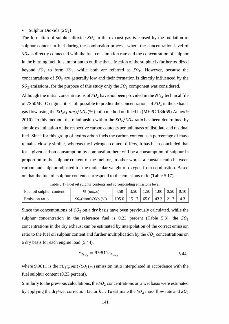
141
• Sulphur Dioxide (𝑆𝑆𝐶𝐶2) The formation of sulphur dioxide 𝑆𝑆𝐶𝐶2 in the exhaust gas is caused by the oxidation of
sulphur content in fuel during the combustion process, where the concentration level of
𝑆𝑆𝐶𝐶2 is directly connected with the fuel consumption rate and the concentration of sulphur
in the burning fuel. It is important to outline that a fraction of the sulphur is further oxidized
beyond 𝑆𝑆𝐶𝐶2 to form 𝑆𝑆𝐶𝐶3, while both are referred as 𝑆𝑆𝐶𝐶𝑋𝑋. However, because the
concentrations of 𝑆𝑆𝐶𝐶3 are generally low and their formation is directly influenced by the
𝑆𝑆𝐶𝐶2 emissions, for the purpose of this study only the 𝑆𝑆𝐶𝐶2 component was considered.
Although the initial concentrations of 𝑆𝑆𝐶𝐶2 have not been provided in the 𝑁𝑁𝐶𝐶𝑋𝑋 technical file
of 7S50MC-C engine, it is still possible to predict the concentrations of 𝑆𝑆𝐶𝐶2 in the exhaust
gas flow using the 𝑆𝑆𝐶𝐶2(𝐶𝐶𝐶𝐶𝑛𝑛) 𝐶𝐶𝐶𝐶2(%)⁄ ratio method outlined in (MEPC.184(59) Annex 9
2010). In this method, the relationship within the 𝑆𝑆𝐶𝐶2 𝐶𝐶𝐶𝐶2⁄ ratio has been determined by
simple examination of the respective carbon contents per unit mass of distillate and residual
fuel. Since for this group of hydrocarbon fuels the carbon content as a percentage of mass
remains closely similar, whereas the hydrogen content differs, it has been concluded that
for a given carbon consumption by combustion there will be a consumption of sulphur in
proportion to the sulphur content of the fuel, or, in other words, a constant ratio between
carbon and sulphur adjusted for the molecular weight of oxygen from combustion. Based
on that the fuel oil sulphur contents correspond to the emissions ratio (Table 5.17).
Table 5.17 Fuel oil sulphur contents and corresponding emissions level.
Fuel oil sulphur content % (𝑛𝑛𝐻𝐻𝑔𝑔𝑔𝑔) 4.50 3.50 1.50 1.00 0.50 0.10
Emission ratio 𝑆𝑆𝐶𝐶2(𝐶𝐶𝐶𝐶𝑛𝑛) 𝐶𝐶𝐶𝐶2(%) ⁄ 195.0 151.7 65.0 43.3 21.7 4.3
Since the concentrations of 𝐶𝐶𝐶𝐶2 on a dry basis have been previously calculated, while the
sulphur concentration in the reference fuel is 0.23 percent (Table 5.3), the 𝑆𝑆𝐶𝐶2
concentrations in the dry exhaust can be estimated by interpolation of the correct emission
ratio to the fuel oil sulphur content and further multiplication by the 𝐶𝐶𝐶𝐶2 concentrations on
a dry basis for each engine load (5.44).
𝐶𝐶𝐴𝐴𝑆𝑆𝐶𝐶2 = 9.9811𝐶𝐶𝐴𝐴𝐶𝐶𝐶𝐶2 5.44
where 9.9811 is the 𝑆𝑆𝐶𝐶2(𝐶𝐶𝐶𝐶𝑛𝑛) 𝐶𝐶𝐶𝐶2(%) ⁄ emission ratio interpolated in accordance with the
fuel sulphur content (0.23 percent).
Similarly to the previous calculations, the 𝑆𝑆𝐶𝐶2 concentrations on a wet basis were estimated
by applying the dry/wet correction factor 𝑘𝑘𝑊𝑊. To estimate the 𝑆𝑆𝐶𝐶2 mass flow rate and 𝑆𝑆𝐶𝐶2
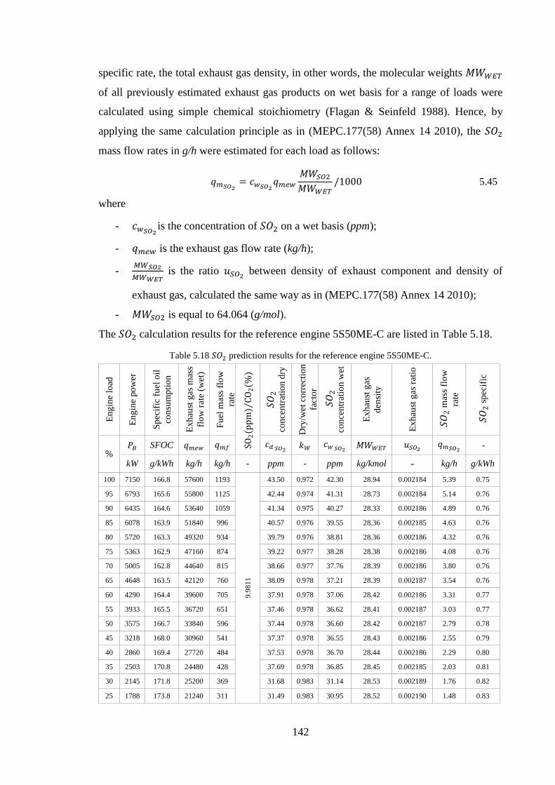
142
specific rate, the total exhaust gas density, in other words, the molecular weights 𝑁𝑁𝑊𝑊𝑊𝑊𝐸𝐸𝑇𝑇
of all previously estimated exhaust gas products on wet basis for a range of loads were
calculated using simple chemical stoichiometry (Flagan & Seinfeld 1988). Hence, by
applying the same calculation principle as in (MEPC.177(58) Annex 14 2010), the 𝑆𝑆𝐶𝐶2
mass flow rates in g/h were estimated for each load as follows:
𝑞𝑞𝑚𝑚𝑆𝑆𝐶𝐶2= 𝐶𝐶𝑤𝑤𝑆𝑆𝐶𝐶2
𝑞𝑞𝑚𝑚𝐴𝐴𝑤𝑤𝑁𝑁𝑊𝑊𝑆𝑆𝑂𝑂2
𝑁𝑁𝑊𝑊𝑊𝑊𝐸𝐸𝑇𝑇/1000 5.45
where
- 𝐶𝐶𝑤𝑤𝑆𝑆𝐶𝐶2is the concentration of 𝑆𝑆𝐶𝐶2 on a wet basis (ppm);
- 𝑞𝑞𝑚𝑚𝐴𝐴𝑤𝑤 is the exhaust gas flow rate (kg/h);
- 𝑀𝑀𝑊𝑊𝑆𝑆𝐶𝐶2𝑀𝑀𝑊𝑊𝑊𝑊𝑀𝑀𝑂𝑂
is the ratio 𝑢𝑢𝑆𝑆𝑂𝑂2 between density of exhaust component and density of
exhaust gas, calculated the same way as in (MEPC.177(58) Annex 14 2010);
- 𝑁𝑁𝑊𝑊𝑆𝑆𝑂𝑂2 is equal to 64.064 (g/mol).
The 𝑆𝑆𝐶𝐶2 calculation results for the reference engine 5S50ME-C are listed in Table 5.18.
Table 5.18 𝑆𝑆𝐶𝐶2 prediction results for the reference engine 5S50ME-C.
Engi
ne lo
ad
Engi
ne p
ower
Spec
ific
fuel
oil
cons
umpt
ion
Exha
ust g
as m
ass
flow
rate
(wet
)
Fuel
mas
s flo
w
rate
SO2(
ppm
)CO
2(%
) ⁄
𝑆𝑆𝐶𝐶2
co
ncen
tratio
n dr
y
Dry
/wet
cor
rect
ion
fact
or
𝑆𝑆𝐶𝐶
2 co
ncen
tratio
n w
et
Exha
ust g
as
dens
ity
Exha
ust g
as ra
tio
𝑆𝑆𝐶𝐶
2 m
ass f
low
ra
te
𝑆𝑆𝐶𝐶
2 sp
ecifi
c
% 𝑃𝑃𝐵𝐵 SFOC 𝑞𝑞𝑚𝑚𝐴𝐴𝑤𝑤 𝑞𝑞𝑚𝑚𝑟𝑟 𝐶𝐶𝐴𝐴 𝑆𝑆𝐶𝐶2
𝑘𝑘𝑊𝑊 𝐶𝐶𝑤𝑤 𝑆𝑆𝐶𝐶2 𝑁𝑁𝑊𝑊𝑊𝑊𝐸𝐸𝑇𝑇 𝑢𝑢𝑆𝑆𝑂𝑂2 𝑞𝑞𝑚𝑚𝑆𝑆𝐶𝐶2
‐
kW g/kWh kg/h kg/h - ppm - ppm kg/kmol - kg/h g/kWh
100 7150 166.8 57600 1193
9.98
11
43.50 0.972 42.30 28.94 0.002184 5.39 0.75
95 6793 165.6 55800 1125 42.44 0.974 41.31 28.73 0.002184 5.14 0.76
90 6435 164.6 53640 1059 41.34 0.975 40.27 28.33 0.002186 4.89 0.76
85 6078 163.9 51840 996 40.57 0.976 39.55 28.36 0.002185 4.63 0.76
80 5720 163.3 49320 934 39.79 0.976 38.81 28.36 0.002186 4.32 0.76
75 5363 162.9 47160 874 39.22 0.977 38.28 28.38 0.002186 4.08 0.76
70 5005 162.8 44640 815 38.66 0.977 37.76 28.39 0.002186 3.80 0.76
65 4648 163.5 42120 760 38.09 0.978 37.21 28.39 0.002187 3.54 0.76
60 4290 164.4 39600 705 37.91 0.978 37.06 28.42 0.002186 3.31 0.77
55 3933 165.5 36720 651 37.46 0.978 36.62 28.41 0.002187 3.03 0.77
50 3575 166.7 33840 596 37.44 0.978 36.60 28.42 0.002187 2.79 0.78
45 3218 168.0 30960 541 37.37 0.978 36.55 28.43 0.002186 2.55 0.79
40 2860 169.4 27720 484 37.53 0.978 36.70 28.44 0.002186 2.29 0.80
35 2503 170.8 24480 428 37.69 0.978 36.85 28.45 0.002185 2.03 0.81
30 2145 171.8 25200 369 31.68 0.983 31.14 28.53 0.002189 1.76 0.82
25 1788 173.8 21240 311 31.49 0.983 30.95 28.52 0.002190 1.48 0.83
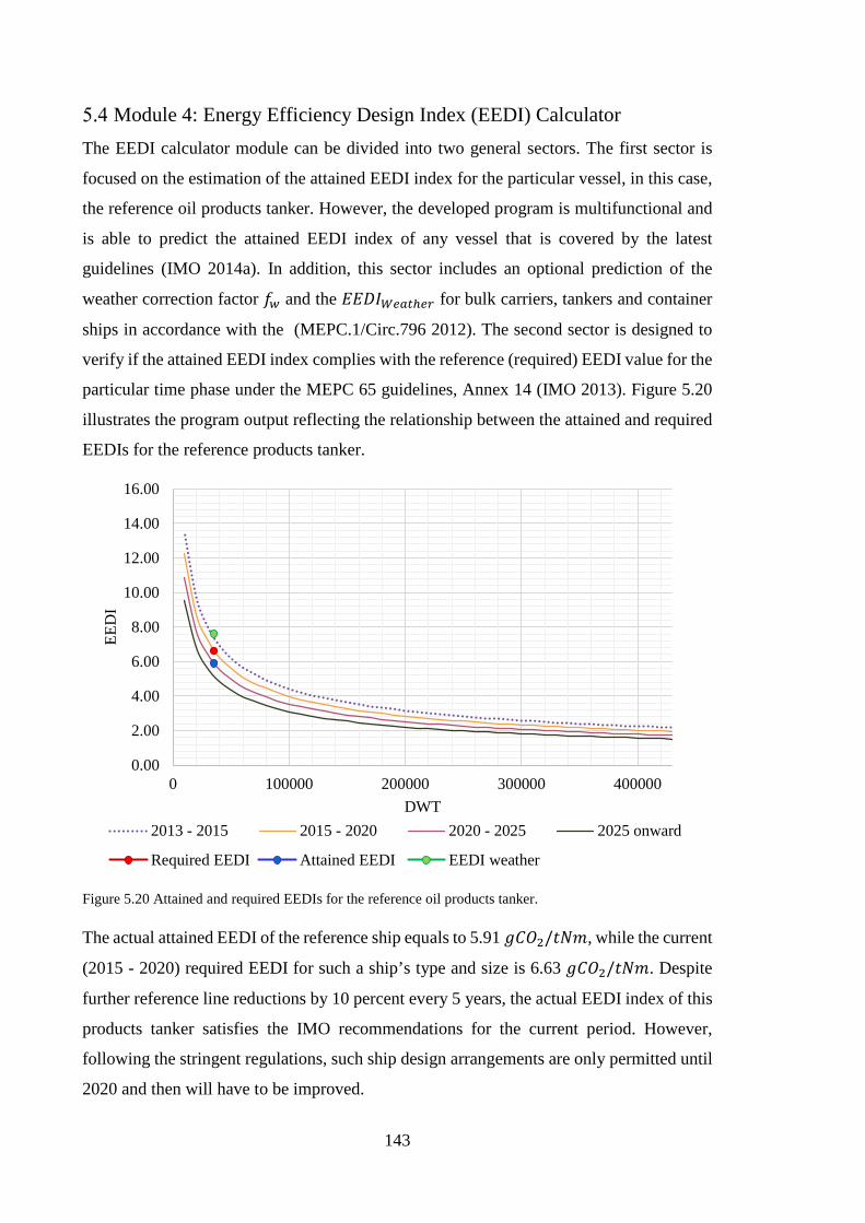
143
Module 4: Energy Efficiency Design Index (EEDI) Calculator The EEDI calculator module can be divided into two general sectors. The first sector is
focused on the estimation of the attained EEDI index for the particular vessel, in this case,
the reference oil products tanker. However, the developed program is multifunctional and
is able to predict the attained EEDI index of any vessel that is covered by the latest
guidelines (IMO 2014a). In addition, this sector includes an optional prediction of the
weather correction factor 𝑓𝑓𝑤𝑤 and the 𝐸𝐸𝐸𝐸𝐷𝐷𝐸𝐸𝑊𝑊𝐴𝐴𝑔𝑔𝐴𝐴ℎ𝐴𝐴𝑟𝑟 for bulk carriers, tankers and container
ships in accordance with the (MEPC.1/Circ.796 2012). The second sector is designed to
verify if the attained EEDI index complies with the reference (required) EEDI value for the
particular time phase under the MEPC 65 guidelines, Annex 14 (IMO 2013). Figure 5.20
illustrates the program output reflecting the relationship between the attained and required
EEDIs for the reference products tanker.
Figure 5.20 Attained and required EEDIs for the reference oil products tanker.
The actual attained EEDI of the reference ship equals to 5.91 𝑔𝑔𝐶𝐶𝐶𝐶2/𝐶𝐶𝑁𝑁𝑛𝑛, while the current
(2015 - 2020) required EEDI for such a ship’s type and size is 6.63 𝑔𝑔𝐶𝐶𝐶𝐶2/𝐶𝐶𝑁𝑁𝑛𝑛. Despite
further reference line reductions by 10 percent every 5 years, the actual EEDI index of this
products tanker satisfies the IMO recommendations for the current period. However,
following the stringent regulations, such ship design arrangements are only permitted until
2020 and then will have to be improved.
0.00
2.00
4.00
6.00
8.00
10.00
12.00
14.00
16.00
0 100000 200000 300000 400000
EED
I
DWT2013 - 2015 2015 - 2020 2020 - 2025 2025 onward
Required EEDI Attained EEDI EEDI weather
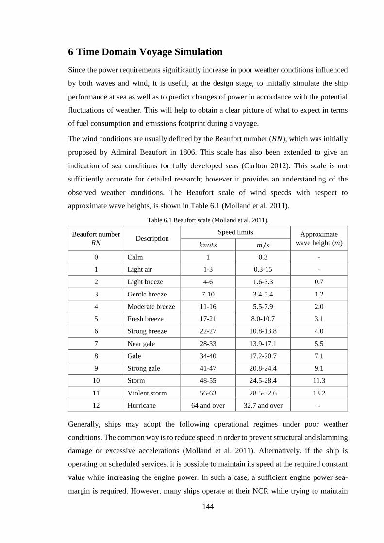
144
6 Time Domain Voyage Simulation
Since the power requirements significantly increase in poor weather conditions influenced
by both waves and wind, it is useful, at the design stage, to initially simulate the ship
performance at sea as well as to predict changes of power in accordance with the potential
fluctuations of weather. This will help to obtain a clear picture of what to expect in terms
of fuel consumption and emissions footprint during a voyage.
The wind conditions are usually defined by the Beaufort number (𝐵𝐵𝑁𝑁), which was initially
proposed by Admiral Beaufort in 1806. This scale has also been extended to give an
indication of sea conditions for fully developed seas (Carlton 2012). This scale is not
sufficiently accurate for detailed research; however it provides an understanding of the
observed weather conditions. The Beaufort scale of wind speeds with respect to
approximate wave heights, is shown in Table 6.1 (Molland et al. 2011).
Table 6.1 Beaufort scale (Molland et al. 2011).
Beaufort number 𝐵𝐵𝑁𝑁 Description
Speed limits Approximate wave height (𝑛𝑛) 𝑘𝑘𝑛𝑛𝑡𝑡𝐶𝐶𝑔𝑔 𝑛𝑛/𝑔𝑔
0 Calm 1 0.3 -
1 Light air 1-3 0.3-15 -
2 Light breeze 4-6 1.6-3.3 0.7
3 Gentle breeze 7-10 3.4-5.4 1.2
4 Moderate breeze 11-16 5.5-7.9 2.0
5 Fresh breeze 17-21 8.0-10.7 3.1
6 Strong breeze 22-27 10.8-13.8 4.0
7 Near gale 28-33 13.9-17.1 5.5
8 Gale 34-40 17.2-20.7 7.1
9 Strong gale 41-47 20.8-24.4 9.1
10 Storm 48-55 24.5-28.4 11.3
11 Violent storm 56-63 28.5-32.6 13.2
12 Hurricane 64 and over 32.7 and over -
Generally, ships may adopt the following operational regimes under poor weather
conditions. The common way is to reduce speed in order to prevent structural and slamming
damage or excessive accelerations (Molland et al. 2011). Alternatively, if the ship is
operating on scheduled services, it is possible to maintain its speed at the required constant
value while increasing the engine power. In such a case, a sufficient engine power sea-
margin is required. However, many ships operate at their NCR while trying to maintain
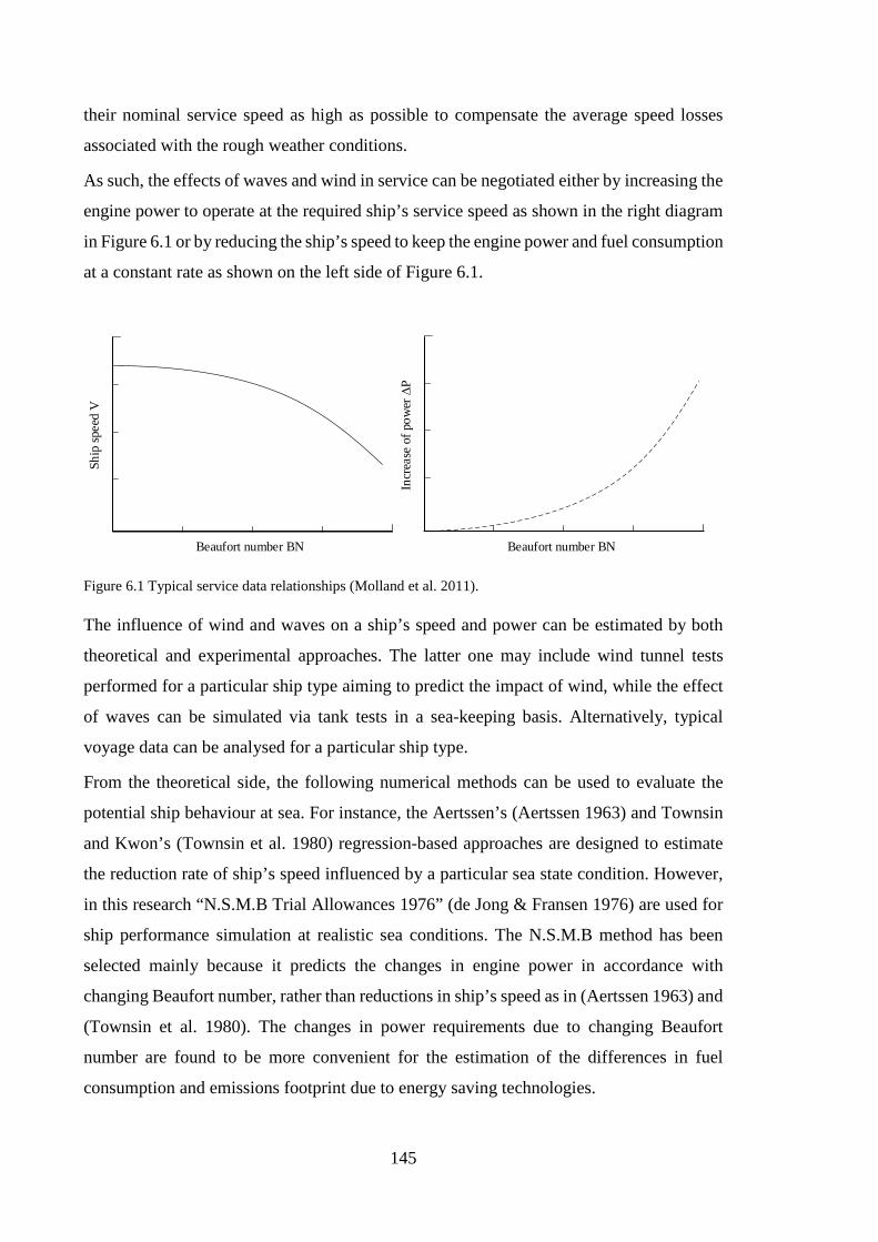
145
their nominal service speed as high as possible to compensate the average speed losses
associated with the rough weather conditions.
As such, the effects of waves and wind in service can be negotiated either by increasing the
engine power to operate at the required ship’s service speed as shown in the right diagram
in Figure 6.1 or by reducing the ship’s speed to keep the engine power and fuel consumption
at a constant rate as shown on the left side of Figure 6.1.
Ship
spee
d V
Beaufort number BN
Incr
ease
of p
ower
∆P
Beaufort number BN
Figure 6.1 Typical service data relationships (Molland et al. 2011).
The influence of wind and waves on a ship’s speed and power can be estimated by both
theoretical and experimental approaches. The latter one may include wind tunnel tests
performed for a particular ship type aiming to predict the impact of wind, while the effect
of waves can be simulated via tank tests in a sea-keeping basis. Alternatively, typical
voyage data can be analysed for a particular ship type.
From the theoretical side, the following numerical methods can be used to evaluate the
potential ship behaviour at sea. For instance, the Aertssen’s (Aertssen 1963) and Townsin
and Kwon’s (Townsin et al. 1980) regression-based approaches are designed to estimate
the reduction rate of ship’s speed influenced by a particular sea state condition. However,
in this research “N.S.M.B Trial Allowances 1976” (de Jong & Fransen 1976) are used for
ship performance simulation at realistic sea conditions. The N.S.M.B method has been
selected mainly because it predicts the changes in engine power in accordance with
changing Beaufort number, rather than reductions in ship’s speed as in (Aertssen 1963) and
(Townsin et al. 1980). The changes in power requirements due to changing Beaufort
number are found to be more convenient for the estimation of the differences in fuel
consumption and emissions footprint due to energy saving technologies.
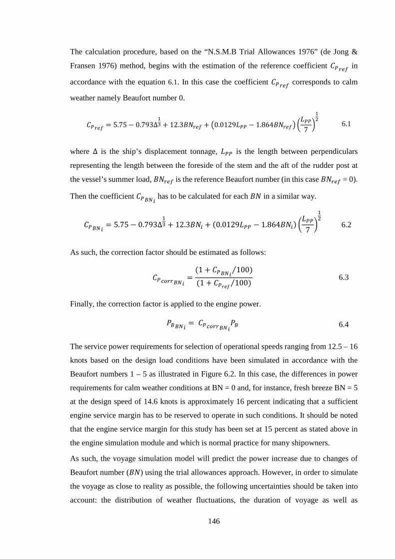
146
The calculation procedure, based on the “N.S.M.B Trial Allowances 1976” (de Jong &
Fransen 1976) method, begins with the estimation of the reference coefficient 𝐶𝐶𝑃𝑃𝑟𝑟𝐴𝐴𝑟𝑟 in
accordance with the equation 6.1. In this case the coefficient 𝐶𝐶𝑃𝑃𝑟𝑟𝐴𝐴𝑟𝑟 corresponds to calm
weather namely Beaufort number 0.
𝐶𝐶𝑃𝑃𝑟𝑟𝐴𝐴𝑟𝑟 = 5.75 − 0.793∆13 + 12.3𝐵𝐵𝑁𝑁𝑟𝑟𝐴𝐴𝑟𝑟 + 0.0129𝐿𝐿𝑃𝑃𝑃𝑃 − 1.864𝐵𝐵𝑁𝑁𝑟𝑟𝐴𝐴𝑟𝑟
𝐿𝐿𝑃𝑃𝑃𝑃712 6.1
where ∆ is the ship’s displacement tonnage, 𝐿𝐿𝑃𝑃𝑃𝑃 is the length between perpendiculars
representing the length between the foreside of the stem and the aft of the rudder post at
the vessel’s summer load, 𝐵𝐵𝑁𝑁𝑟𝑟𝐴𝐴𝑟𝑟 is the reference Beaufort number (in this case 𝐵𝐵𝑁𝑁𝑟𝑟𝐴𝐴𝑟𝑟 = 0).
Then the coefficient 𝐶𝐶𝑃𝑃𝐵𝐵𝑆𝑆𝐴𝐴 has to be calculated for each 𝐵𝐵𝑁𝑁 in a similar way.
𝐶𝐶𝑃𝑃𝐵𝐵𝑆𝑆𝐴𝐴 = 5.75 − 0.793∆13 + 12.3𝐵𝐵𝑁𝑁𝐴𝐴 + (0.0129𝐿𝐿𝑃𝑃𝑃𝑃 − 1.864𝐵𝐵𝑁𝑁𝐴𝐴)
𝐿𝐿𝑃𝑃𝑃𝑃712 6.2
As such, the correction factor should be estimated as follows:
𝐶𝐶𝑃𝑃𝑐𝑐𝑏𝑏𝑟𝑟𝑟𝑟𝐵𝐵𝑆𝑆𝐴𝐴=
(1 + 𝐶𝐶𝑃𝑃𝐵𝐵𝑆𝑆𝐴𝐴 100⁄ )(1 + 𝐶𝐶𝑃𝑃𝑟𝑟𝑟𝑟𝑟𝑟 100⁄ )
6.3
Finally, the correction factor is applied to the engine power.
𝑃𝑃𝐵𝐵𝐵𝐵𝑆𝑆𝐴𝐴 = 𝐶𝐶𝑃𝑃𝑐𝑐𝑏𝑏𝑟𝑟𝑟𝑟𝐵𝐵𝑆𝑆𝐴𝐴𝑃𝑃𝐵𝐵 6.4
The service power requirements for selection of operational speeds ranging from 12.5 – 16
knots based on the design load conditions have been simulated in accordance with the
Beaufort numbers 1 – 5 as illustrated in Figure 6.2. In this case, the differences in power
requirements for calm weather conditions at BN = 0 and, for instance, fresh breeze BN = 5
at the design speed of 14.6 knots is approximately 16 percent indicating that a sufficient
engine service margin has to be reserved to operate in such conditions. It should be noted
that the engine service margin for this study has been set at 15 percent as stated above in
the engine simulation module and which is normal practice for many shipowners.
As such, the voyage simulation model will predict the power increase due to changes of
Beaufort number (𝐵𝐵𝑁𝑁) using the trial allowances approach. However, in order to simulate
the voyage as close to reality as possible, the following uncertainties should be taken into
account: the distribution of weather fluctuations, the duration of voyage as well as
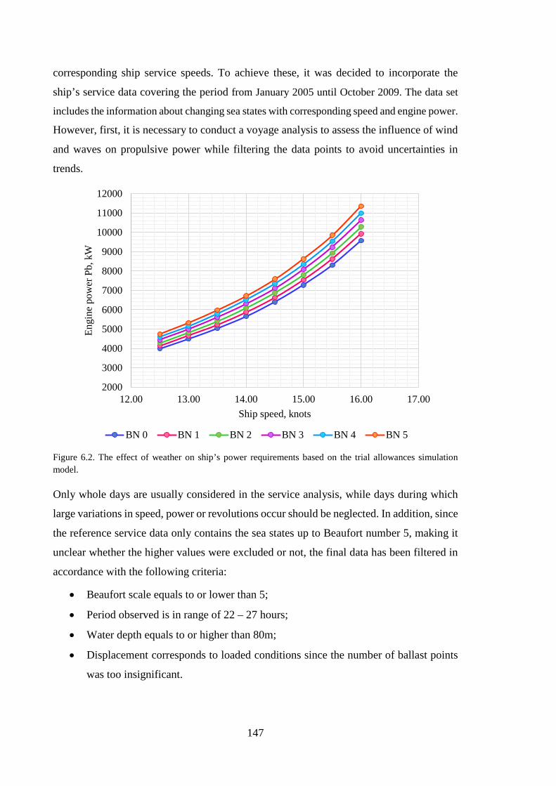
147
corresponding ship service speeds. To achieve these, it was decided to incorporate the
ship’s service data covering the period from January 2005 until October 2009. The data set
includes the information about changing sea states with corresponding speed and engine power.
However, first, it is necessary to conduct a voyage analysis to assess the influence of wind
and waves on propulsive power while filtering the data points to avoid uncertainties in
trends.
Figure 6.2. The effect of weather on ship’s power requirements based on the trial allowances simulation model.
Only whole days are usually considered in the service analysis, while days during which
large variations in speed, power or revolutions occur should be neglected. In addition, since
the reference service data only contains the sea states up to Beaufort number 5, making it
unclear whether the higher values were excluded or not, the final data has been filtered in
accordance with the following criteria:
• Beaufort scale equals to or lower than 5;
• Period observed is in range of 22 – 27 hours;
• Water depth equals to or higher than 80m;
• Displacement corresponds to loaded conditions since the number of ballast points
was too insignificant.
2000
3000
4000
5000
6000
7000
8000
9000
10000
11000
12000
12.00 13.00 14.00 15.00 16.00 17.00
Engi
ne p
ower
Pb,
kW
Ship speed, knots
BN 0 BN 1 BN 2 BN 3 BN 4 BN 5
148
Changes of displacement were obtained via the regression analysis of the measured mean
draughts compared with the draughts available in the model test report and associated with
them displacements. In addition, since the ship’s speed measured through water using
shipborne logs can be inaccurate due to the influence of the boundary layer, ship motions
or tide (Molland et al. 2011), only the speeds observed via the Global Positioning System
(GPS) are considered.
As outlined in (Carlton 2012), by analysing the relationship between the Admiralty
coefficient 𝐵𝐵𝐶𝐶 (equation 6.5) and the apparent slip 𝑆𝑆𝑔𝑔 (equation 6.6) as shown in Figure
6.3, it is possible to detect potential outliers among the observations as well as to assess the
data quality, since 𝐵𝐵𝐶𝐶 – 𝑆𝑆𝑔𝑔 relationship represents a convergence in the data.
𝐵𝐵𝐶𝐶 =∆2 3 𝑁𝑁𝑆𝑆3
𝑃𝑃𝐵𝐵 6.5
where ∆ is the displacement, 𝑁𝑁𝑆𝑆 is the speed and 𝑃𝑃𝐵𝐵 is the engine power.
𝑆𝑆𝑔𝑔 = 1 − 30.86 𝑁𝑁𝑆𝑆𝑃𝑃𝑁𝑁
6.6
where 𝑃𝑃 is the propeller pitch, 𝑁𝑁 is the rotational speed, while 𝑁𝑁𝑆𝑆 is defined in m/s.
Figure 6.3 Unfiltered Admiralty coefficient versus apparent slip.
Several data points from the observations, that weren’t fitting well into the convergence,
were carefully examined and, if a discrepancy detected, the outliers were removed from the
R² = 0.6144
0
100
200
300
400
500
600
700
800
-15 -10 -5 0 5 10 15
Adm
iralty
coe
ffic
ient
Apparent slip
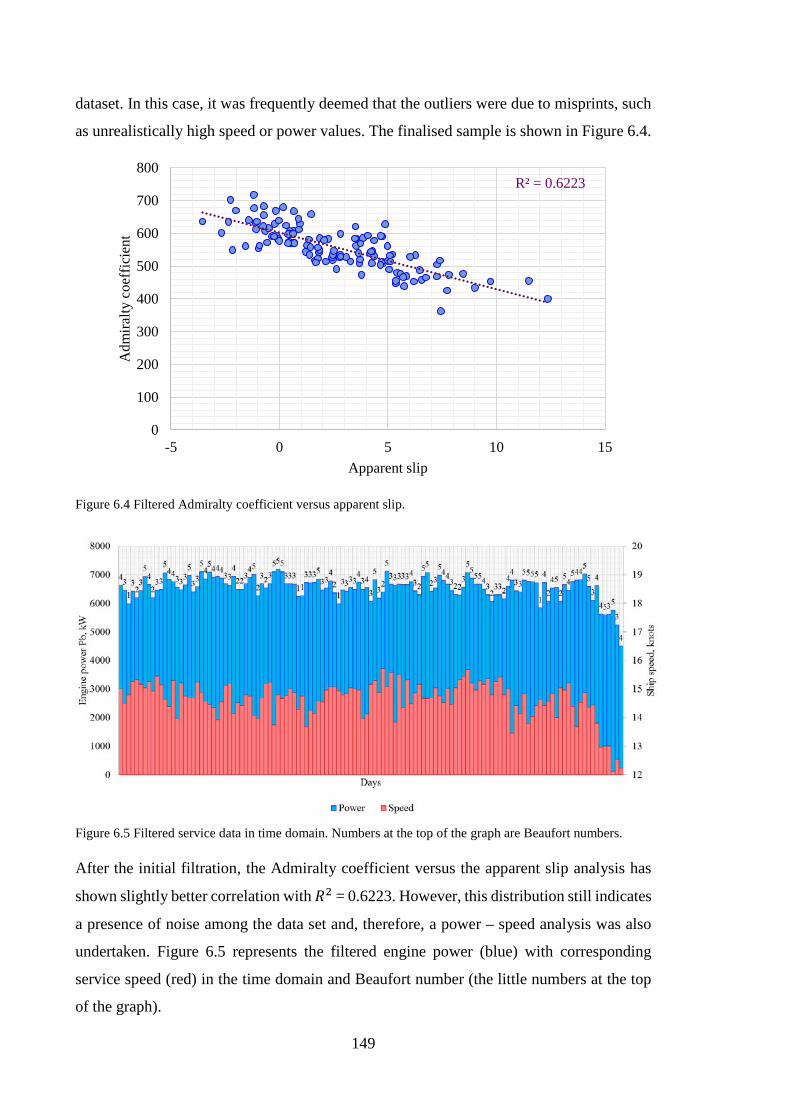
149
dataset. In this case, it was frequently deemed that the outliers were due to misprints, such
as unrealistically high speed or power values. The finalised sample is shown in Figure 6.4.
Figure 6.4 Filtered Admiralty coefficient versus apparent slip.
Figure 6.5 Filtered service data in time domain. Numbers at the top of the graph are Beaufort numbers.
After the initial filtration, the Admiralty coefficient versus the apparent slip analysis has
shown slightly better correlation with 𝐵𝐵2 = 0.6223. However, this distribution still indicates
a presence of noise among the data set and, therefore, a power – speed analysis was also
undertaken. Figure 6.5 represents the filtered engine power (blue) with corresponding
service speed (red) in the time domain and Beaufort number (the little numbers at the top
of the graph).
R² = 0.6223
0
100
200
300
400
500
600
700
800
-5 0 5 10 15
Adm
iralty
coe
ffic
ient
Apparent slip
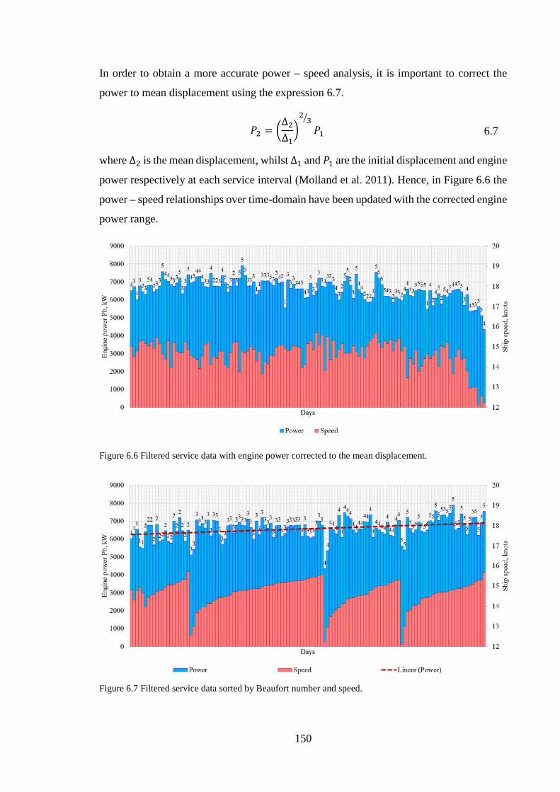
150
In order to obtain a more accurate power – speed analysis, it is important to correct the
power to mean displacement using the expression 6.7.
𝑃𝑃2 = ∆2∆123
𝑃𝑃1 6.7
where ∆2 is the mean displacement, whilst ∆1 and 𝑃𝑃1 are the initial displacement and engine
power respectively at each service interval (Molland et al. 2011). Hence, in Figure 6.6 the
power – speed relationships over time-domain have been updated with the corrected engine
power range.
Figure 6.6 Filtered service data with engine power corrected to the mean displacement.
Figure 6.7 Filtered service data sorted by Beaufort number and speed.
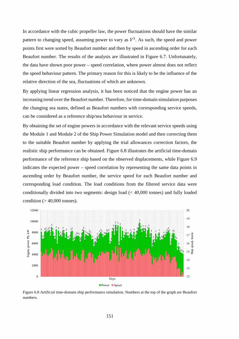
151
In accordance with the cubic propeller law, the power fluctuations should have the similar
pattern to changing speed, assuming power to vary as 𝑁𝑁3. As such, the speed and power
points first were sorted by Beaufort number and then by speed in ascending order for each
Beaufort number. The results of the analysis are illustrated in Figure 6.7. Unfortunately,
the data have shown poor power – speed correlation, where power almost does not reflect
the speed behaviour pattern. The primary reason for this is likely to be the influence of the
relative direction of the sea, fluctuations of which are unknown.
By applying linear regression analysis, it has been noticed that the engine power has an
increasing trend over the Beaufort number. Therefore, for time-domain simulation purposes
the changing sea states, defined as Beaufort numbers with corresponding service speeds,
can be considered as a reference ship/sea behaviour in service.
By obtaining the set of engine powers in accordance with the relevant service speeds using
the Module 1 and Module 2 of the Ship Power Simulation model and then correcting them
to the suitable Beaufort number by applying the trial allowances correction factors, the
realistic ship performance can be obtained. Figure 6.8 illustrates the artificial time-domain
performance of the reference ship based on the observed displacements, while Figure 6.9
indicates the expected power – speed correlation by representing the same data points in
ascending order by Beaufort number, the service speed for each Beaufort number and
corresponding load condition. The load conditions from the filtered service data were
conditionally divided into two segments: design load (< 40,000 tonnes) and fully loaded
condition (> 40,000 tonnes).
Figure 6.8 Artificial time-domain ship performance simulation. Numbers at the top of the graph are Beaufort numbers.
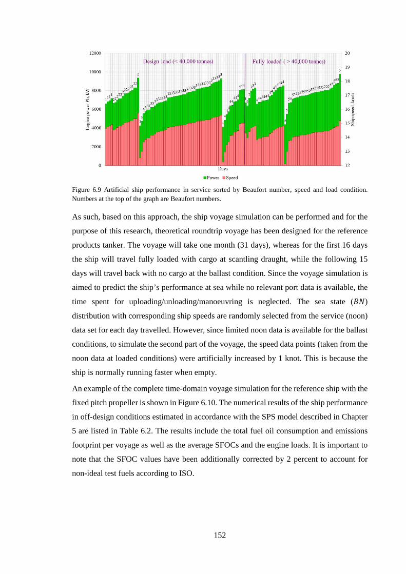
152
Figure 6.9 Artificial ship performance in service sorted by Beaufort number, speed and load condition. Numbers at the top of the graph are Beaufort numbers.
As such, based on this approach, the ship voyage simulation can be performed and for the
purpose of this research, theoretical roundtrip voyage has been designed for the reference
products tanker. The voyage will take one month (31 days), whereas for the first 16 days
the ship will travel fully loaded with cargo at scantling draught, while the following 15
days will travel back with no cargo at the ballast condition. Since the voyage simulation is
aimed to predict the ship’s performance at sea while no relevant port data is available, the
time spent for uploading/unloading/manoeuvring is neglected. The sea state (𝐵𝐵𝑁𝑁)
distribution with corresponding ship speeds are randomly selected from the service (noon)
data set for each day travelled. However, since limited noon data is available for the ballast
conditions, to simulate the second part of the voyage, the speed data points (taken from the
noon data at loaded conditions) were artificially increased by 1 knot. This is because the
ship is normally running faster when empty.
An example of the complete time-domain voyage simulation for the reference ship with the
fixed pitch propeller is shown in Figure 6.10. The numerical results of the ship performance
in off-design conditions estimated in accordance with the SPS model described in Chapter
5 are listed in Table 6.2. The results include the total fuel oil consumption and emissions
footprint per voyage as well as the average SFOCs and the engine loads. It is important to
note that the SFOC values have been additionally corrected by 2 percent to account for
non-ideal test fuels according to ISO.
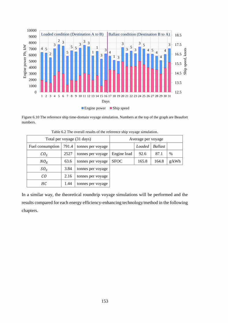
153
Figure 6.10 The reference ship time-domain voyage simulation. Numbers at the top of the graph are Beaufort numbers.
Table 6.2 The overall results of the reference ship voyage simulation.
Total per voyage (31 days) Average per voyage
Fuel consumption 791.4 tonnes per voyage Loaded Ballast
𝐶𝐶𝐶𝐶2 2527 tonnes per voyage Engine load 92.6 87.1 %
𝑁𝑁𝐶𝐶𝑋𝑋 63.6 tonnes per voyage SFOC 165.8 164.8 g/kWh
𝑆𝑆𝐶𝐶2 3.84 tonnes per voyage
𝐶𝐶𝐶𝐶 2.16 tonnes per voyage
𝐻𝐻𝐶𝐶 1.44 tonnes per voyage
In a similar way, the theoretical roundtrip voyage simulations will be performed and the
results compared for each energy efficiency-enhancing technology/method in the following
chapters.
4 52
32 3
55 5
33 3
11
33 4
1 3
33 5
3
3 54 5 4
44
3
12.5
13.5
14.5
15.5
16.5
17.5
18.5
0100020003000400050006000700080009000
10000
1 2 3 4 5 6 7 8 9 10 11 12 13 14 15 16 17 18 19 20 21 22 23 24 25 26 27 28 29 30 31
Ship
spee
d, k
nots
Engi
ne p
ower
Pb,
kW
Days
Engine power Ship speed
Loaded condition (Destination A to B) Ballast condition (Destination B to A)
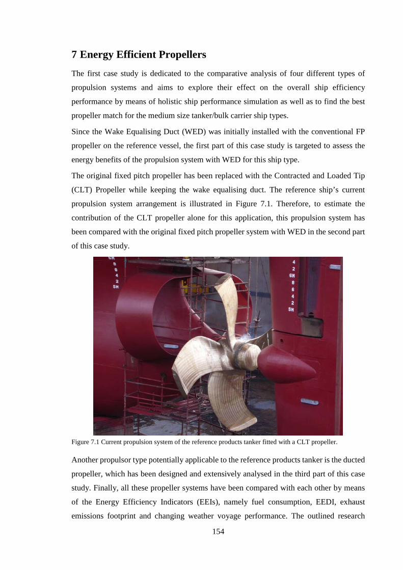
154
7 Energy Efficient Propellers
The first case study is dedicated to the comparative analysis of four different types of
propulsion systems and aims to explore their effect on the overall ship efficiency
performance by means of holistic ship performance simulation as well as to find the best
propeller match for the medium size tanker/bulk carrier ship types.
Since the Wake Equalising Duct (WED) was initially installed with the conventional FP
propeller on the reference vessel, the first part of this case study is targeted to assess the
energy benefits of the propulsion system with WED for this ship type.
The original fixed pitch propeller has been replaced with the Contracted and Loaded Tip
(CLT) Propeller while keeping the wake equalising duct. The reference ship’s current
propulsion system arrangement is illustrated in Figure 7.1. Therefore, to estimate the
contribution of the CLT propeller alone for this application, this propulsion system has
been compared with the original fixed pitch propeller system with WED in the second part
of this case study.
Figure 7.1 Current propulsion system of the reference products tanker fitted with a CLT propeller.
Another propulsor type potentially applicable to the reference products tanker is the ducted
propeller, which has been designed and extensively analysed in the third part of this case
study. Finally, all these propeller systems have been compared with each other by means
of the Energy Efficiency Indicators (EEIs), namely fuel consumption, EEDI, exhaust
emissions footprint and changing weather voyage performance. The outlined research
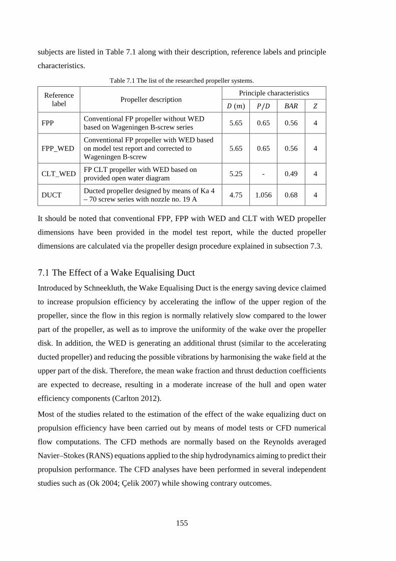
155
subjects are listed in Table 7.1 along with their description, reference labels and principle
characteristics.
Table 7.1 The list of the researched propeller systems.
Reference label Propeller description
Principle characteristics
𝐷𝐷 (𝑛𝑛) 𝑃𝑃/𝐷𝐷 BAR 𝑍𝑍
FPP Conventional FP propeller without WED based on Wageningen B-screw series 5.65 0.65 0.56 4
FPP_WED Conventional FP propeller with WED based on model test report and corrected to Wageningen B-screw
5.65 0.65 0.56 4
CLT_WED FP CLT propeller with WED based on provided open water diagram 5.25 - 0.49 4
DUCT Ducted propeller designed by means of Ka 4 – 70 screw series with nozzle no. 19 A 4.75 1.056 0.68 4
It should be noted that conventional FPP, FPP with WED and CLT with WED propeller
dimensions have been provided in the model test report, while the ducted propeller
dimensions are calculated via the propeller design procedure explained in subsection 7.3.
The Effect of a Wake Equalising Duct Introduced by Schneekluth, the Wake Equalising Duct is the energy saving device claimed
to increase propulsion efficiency by accelerating the inflow of the upper region of the
propeller, since the flow in this region is normally relatively slow compared to the lower
part of the propeller, as well as to improve the uniformity of the wake over the propeller
disk. In addition, the WED is generating an additional thrust (similar to the accelerating
ducted propeller) and reducing the possible vibrations by harmonising the wake field at the
upper part of the disk. Therefore, the mean wake fraction and thrust deduction coefficients
are expected to decrease, resulting in a moderate increase of the hull and open water
efficiency components (Carlton 2012).
Most of the studies related to the estimation of the effect of the wake equalizing duct on
propulsion efficiency have been carried out by means of model tests or CFD numerical
flow computations. The CFD methods are normally based on the Reynolds averaged
Navier–Stokes (RANS) equations applied to the ship hydrodynamics aiming to predict their
propulsion performance. The CFD analyses have been performed in several independent
studies such as (Ok 2004; Çelik 2007) while showing contrary outcomes.
156
The (Ok 2004) study is dedicated to the effect of the WED installed on the tanker with a
higher block coefficient while the numerical computations are performed using the CFD
code based on finite volume method. In (Ok 2004), the Reynolds number effects have been
investigated for various ship speeds without the propeller presence at the after body. The
results have shown a moderate frictional resistance increase and, thus, additional power
requirements for propulsion due to the presence of the WED, compared to the naked hull.
In (Çelik 2007), a numerical investigation based on RANS method has been carried out to
find the most appropriate wake equalizing duct arrangement for a chemical tanker. The
computations are carried out for the ship alone, the ship with a propeller, the ship with a
wake equalizing duct alone and the ship with a wake equalizing duct and a propeller for the
speed range of 10 – 16 knots. As a result, it was found that the differences in the frictional
and the viscous pressure resistances between ships with and without WED were
insignificant for all the cases. It was also found that the maximum efficiency gain obtained
with the relevant WED design is about 10 percent mainly due to additionally generated
thrust. It is likely, however, that the results of both studies were highly influenced by the
turbulence model used in the computations.
Regarding the WED studies based on model tests, it is difficult to accurately extrapolate
the powering performance to the actual full scale, especially for larger vessels, due to the
Reynolds number scale effects. The reason is that WED installations are normally fitted to
very large ships, which results in a relatively low towing speed in the tank to comply with
Froude number scaling of the full-scale ship speed. To address these issues further reliable
correlations are needed including tests done in large cavitation tunnels at higher speeds;
towing tank tests performed for some equivalent speeds at the lower end of the cavitation
tunnel range; and full-scale trials results (ITTC 1999).
For this study, the reference ship’s model test report contains self-propulsion tests of the
system with a WED for design, loaded and ballast conditions extrapolated to the full scale.
These full-scale powering performance results, of course, might be less accurate than the
full-scale trials. However, since the reference ship is rather on the smaller side of the
spectrum of ship sizes suitable for the WED installation, this analysis may shed some
further information into the potential efficiency benefits that could be expected with the
installation of a WED for ships of the reference type and size. This, however, recognises
the difference in local Reynolds number between the WED and a hull: the former working
within the boundary layer of the latter.
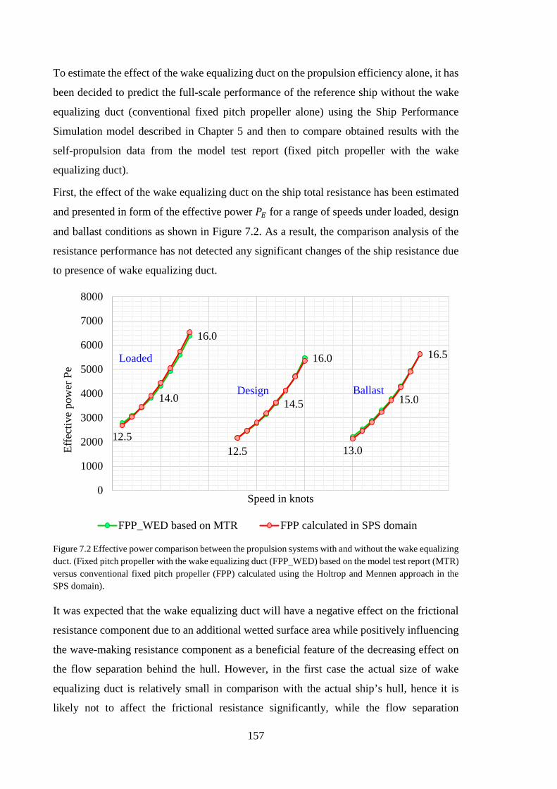
157
To estimate the effect of the wake equalizing duct on the propulsion efficiency alone, it has
been decided to predict the full-scale performance of the reference ship without the wake
equalizing duct (conventional fixed pitch propeller alone) using the Ship Performance
Simulation model described in Chapter 5 and then to compare obtained results with the
self-propulsion data from the model test report (fixed pitch propeller with the wake
equalizing duct).
First, the effect of the wake equalizing duct on the ship total resistance has been estimated
and presented in form of the effective power 𝑃𝑃𝐸𝐸 for a range of speeds under loaded, design
and ballast conditions as shown in Figure 7.2. As a result, the comparison analysis of the
resistance performance has not detected any significant changes of the ship resistance due
to presence of wake equalizing duct.
Figure 7.2 Effective power comparison between the propulsion systems with and without the wake equalizing duct. (Fixed pitch propeller with the wake equalizing duct (FPP_WED) based on the model test report (MTR) versus conventional fixed pitch propeller (FPP) calculated using the Holtrop and Mennen approach in the SPS domain).
It was expected that the wake equalizing duct will have a negative effect on the frictional
resistance component due to an additional wetted surface area while positively influencing
the wave-making resistance component as a beneficial feature of the decreasing effect on
the flow separation behind the hull. However, in the first case the actual size of wake
equalizing duct is relatively small in comparison with the actual ship’s hull, hence it is
likely not to affect the frictional resistance significantly, while the flow separation
12.5
14.0
16.0
12.5
14.5
16.0
13.0
15.0
16.5
0
1000
2000
3000
4000
5000
6000
7000
8000
Effe
ctiv
e po
wer
Pe
Speed in knots
FPP_WED based on MTR FPP calculated in SPS domain
Loaded
Design Ballast
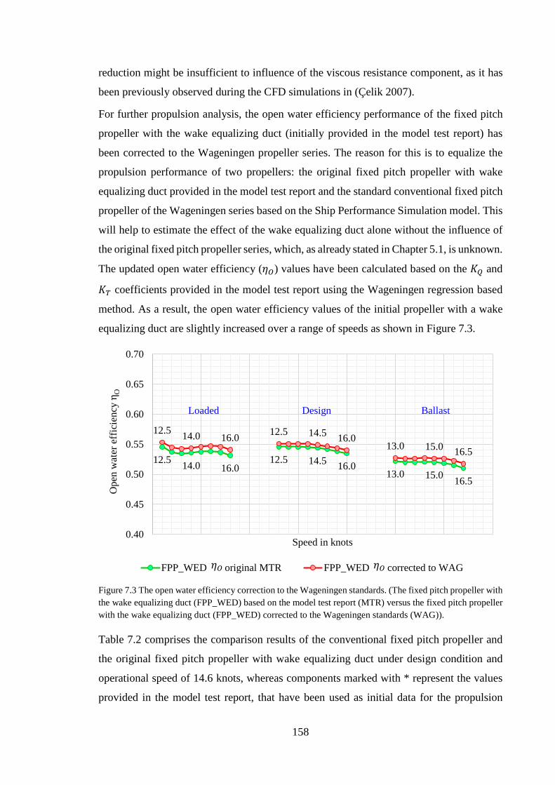
158
reduction might be insufficient to influence of the viscous resistance component, as it has
been previously observed during the CFD simulations in (Çelik 2007).
For further propulsion analysis, the open water efficiency performance of the fixed pitch
propeller with the wake equalizing duct (initially provided in the model test report) has
been corrected to the Wageningen propeller series. The reason for this is to equalize the
propulsion performance of two propellers: the original fixed pitch propeller with wake
equalizing duct provided in the model test report and the standard conventional fixed pitch
propeller of the Wageningen series based on the Ship Performance Simulation model. This
will help to estimate the effect of the wake equalizing duct alone without the influence of
the original fixed pitch propeller series, which, as already stated in Chapter 5.1, is unknown.
The updated open water efficiency (𝜂𝜂𝑂𝑂) values have been calculated based on the 𝐾𝐾𝑄𝑄 and
𝐾𝐾𝑇𝑇 coefficients provided in the model test report using the Wageningen regression based
method. As a result, the open water efficiency values of the initial propeller with a wake
equalizing duct are slightly increased over a range of speeds as shown in Figure 7.3.
Figure 7.3 The open water efficiency correction to the Wageningen standards. (The fixed pitch propeller with the wake equalizing duct (FPP_WED) based on the model test report (MTR) versus the fixed pitch propeller with the wake equalizing duct (FPP_WED) corrected to the Wageningen standards (WAG)).
Table 7.2 comprises the comparison results of the conventional fixed pitch propeller and
the original fixed pitch propeller with wake equalizing duct under design condition and
operational speed of 14.6 knots, whereas components marked with * represent the values
provided in the model test report, that have been used as initial data for the propulsion
12.5 14.0 16.012.5 14.5 16.0
13.0 15.0 16.5
12.5 14.0 16.0 12.5 14.5 16.013.0 15.0 16.5
0.40
0.45
0.50
0.55
0.60
0.65
0.70
Ope
n w
ater
eff
icie
ncy
η O
Speed in knots
FPP_WED original MTR FPP_WED corrected to WAG
Loaded Design Ballast
𝜂𝜂𝑂𝑂 𝜂𝜂𝑂𝑂
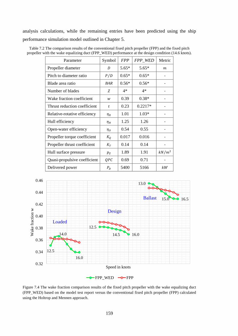
159
analysis calculations, while the remaining entries have been predicted using the ship
performance simulation model outlined in Chapter 5.
Table 7.2 The comparison results of the conventional fixed pitch propeller (FPP) and the fixed pitch propeller with the wake equalizing duct (FPP_WED) performance at the design condition (14.6 knots).
Parameter Symbol FPP FPP_WED Metric
Propeller diameter 𝐷𝐷 5.65* 5.65* 𝑛𝑛
Pitch to diameter ratio 𝑃𝑃 𝐷𝐷⁄ 0.65* 0.65* -
Blade area ratio BAR 0.56* 0.56* -
Number of blades 𝑍𝑍 4* 4* -
Wake fraction coefficient 𝑤𝑤 0.39 0.38* -
Thrust reduction coefficient 𝐶𝐶 0.23 0.2217* -
Relative-rotative efficiency 𝜂𝜂𝑅𝑅 1.01 1.03* -
Hull efficiency 𝜂𝜂𝐻𝐻 1.25 1.26 -
Open-water efficiency 𝜂𝜂𝑂𝑂 0.54 0.55 -
Propeller torque coefficient 𝐾𝐾𝑄𝑄 0.017 0.016 -
Propeller thrust coefficient 𝐾𝐾𝑇𝑇 0.14 0.14 -
Hull surface pressure 𝐶𝐶𝑍𝑍 1.89 1.91 𝑘𝑘𝑁𝑁 𝑛𝑛2⁄
Quasi-propulsive coefficient 𝑄𝑄𝑃𝑃𝐶𝐶 0.69 0.71 -
Delivered power 𝑃𝑃𝐷𝐷 5400 5166 𝑘𝑘𝑊𝑊
Figure 7.4 The wake fraction comparison results of the fixed pitch propeller with the wake equalizing duct (FPP_WED) based on the model test report versus the conventional fixed pitch propeller (FPP) calculated using the Holtrop and Mennen approach.
12.5
14.0
16.0
12.5
14.5 16.0
13.0
15.0 16.5
0.32
0.34
0.36
0.38
0.40
0.42
0.44
0.46
Wak
e fra
ctio
n w
Speed in knots
FPP_WED FPP
Loaded
Design
Ballast
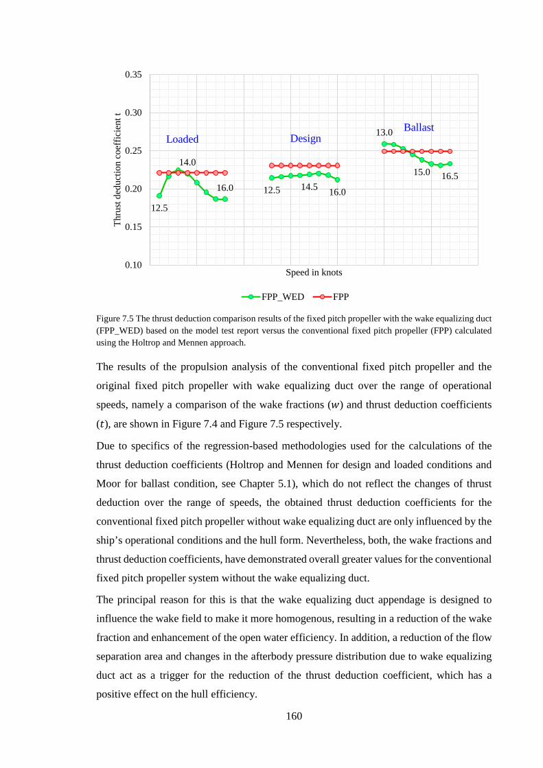
160
Figure 7.5 The thrust deduction comparison results of the fixed pitch propeller with the wake equalizing duct (FPP_WED) based on the model test report versus the conventional fixed pitch propeller (FPP) calculated using the Holtrop and Mennen approach.
The results of the propulsion analysis of the conventional fixed pitch propeller and the
original fixed pitch propeller with wake equalizing duct over the range of operational
speeds, namely a comparison of the wake fractions (𝑤𝑤) and thrust deduction coefficients
(𝐶𝐶), are shown in Figure 7.4 and Figure 7.5 respectively.
Due to specifics of the regression-based methodologies used for the calculations of the
thrust deduction coefficients (Holtrop and Mennen for design and loaded conditions and
Moor for ballast condition, see Chapter 5.1), which do not reflect the changes of thrust
deduction over the range of speeds, the obtained thrust deduction coefficients for the
conventional fixed pitch propeller without wake equalizing duct are only influenced by the
ship’s operational conditions and the hull form. Nevertheless, both, the wake fractions and
thrust deduction coefficients, have demonstrated overall greater values for the conventional
fixed pitch propeller system without the wake equalizing duct.
The principal reason for this is that the wake equalizing duct appendage is designed to
influence the wake field to make it more homogenous, resulting in a reduction of the wake
fraction and enhancement of the open water efficiency. In addition, a reduction of the flow
separation area and changes in the afterbody pressure distribution due to wake equalizing
duct act as a trigger for the reduction of the thrust deduction coefficient, which has a
positive effect on the hull efficiency.
12.5
14.0
16.0 12.5 14.5 16.0
13.0
15.0 16.5
0.10
0.15
0.20
0.25
0.30
0.35
Thru
st de
duct
ion
coef
ficie
nt t
Speed in knots
FPP_WED FPP
Loaded DesignBallast
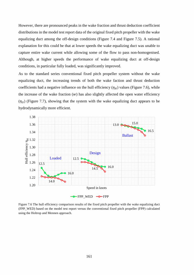
161
However, there are pronounced peaks in the wake fraction and thrust deduction coefficient
distributions in the model test report data of the original fixed pitch propeller with the wake
equalizing duct among the off-design conditions (Figure 7.4 and Figure 7.5). A rational
explanation for this could be that at lower speeds the wake equalizing duct was unable to
capture entire wake current while allowing some of the flow to pass non-homogenised.
Although, at higher speeds the performance of wake equalizing duct at off-design
conditions, in particular fully loaded, was significantly improved.
As to the standard series conventional fixed pitch propeller system without the wake
equalizing duct, the increasing trends of both the wake faction and thrust deduction
coefficients had a negative influence on the hull efficiency (𝜂𝜂𝐻𝐻) values (Figure 7.6), while
the increase of the wake fraction (𝑤𝑤) has also slightly affected the open water efficiency
(𝜂𝜂𝑂𝑂) (Figure 7.7), showing that the system with the wake equalizing duct appears to be
hydrodynamically more efficient.
Figure 7.6 The hull efficiency comparison results of the fixed pitch propeller with the wake equalizing duct (FPP_WED) based on the model test report versus the conventional fixed pitch propeller (FPP) calculated using the Holtrop and Mennen approach.
12.5
14.0
16.0
12.5
14.5 16.0
13.0 15.0
16.5
1.20
1.22
1.24
1.26
1.28
1.30
1.32
1.34
1.36
1.38
Hul
l effi
cien
cy η
H
Speed in knots
FPP_WED FPP
LoadedDesign
Ballast
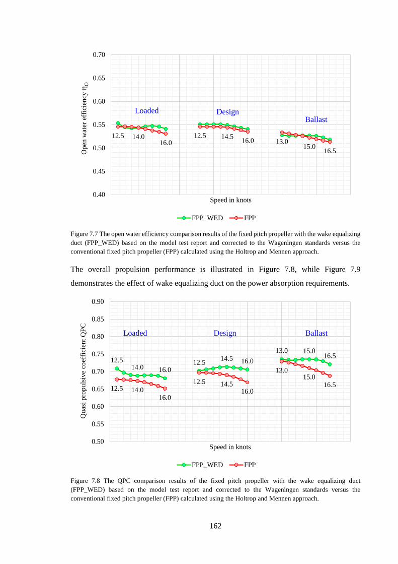
162
Figure 7.7 The open water efficiency comparison results of the fixed pitch propeller with the wake equalizing duct (FPP_WED) based on the model test report and corrected to the Wageningen standards versus the conventional fixed pitch propeller (FPP) calculated using the Holtrop and Mennen approach.
The overall propulsion performance is illustrated in Figure 7.8, while Figure 7.9
demonstrates the effect of wake equalizing duct on the power absorption requirements.
Figure 7.8 The QPC comparison results of the fixed pitch propeller with the wake equalizing duct (FPP_WED) based on the model test report and corrected to the Wageningen standards versus the conventional fixed pitch propeller (FPP) calculated using the Holtrop and Mennen approach.
12.5 14.016.0
12.5 14.5 16.0 13.015.0 16.5
0.40
0.45
0.50
0.55
0.60
0.65
0.70
Ope
n w
ater
effi
cien
cy η
O
Speed in knots
FPP_WED FPP
Loaded DesignBallast
12.514.0 16.0
12.5 14.5 16.013.0 15.0
16.5
12.5 14.016.0
12.5 14.516.0
13.015.0
16.5
0.50
0.55
0.60
0.65
0.70
0.75
0.80
0.85
0.90
Qua
si pr
opul
sive
coef
ficie
nt Q
PC
Speed in knots
FPP_WED FPP
Loaded Design Ballast
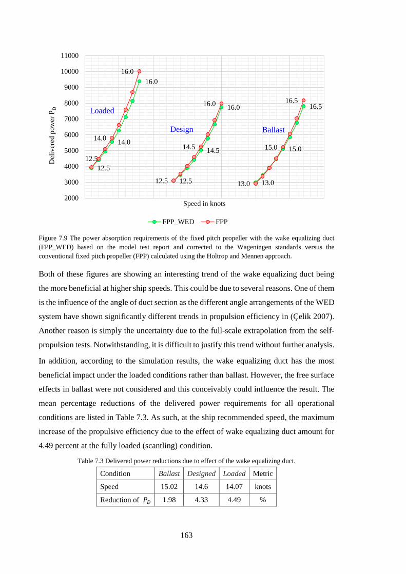
163
Figure 7.9 The power absorption requirements of the fixed pitch propeller with the wake equalizing duct (FPP_WED) based on the model test report and corrected to the Wageningen standards versus the conventional fixed pitch propeller (FPP) calculated using the Holtrop and Mennen approach.
Both of these figures are showing an interesting trend of the wake equalizing duct being
the more beneficial at higher ship speeds. This could be due to several reasons. One of them
is the influence of the angle of duct section as the different angle arrangements of the WED
system have shown significantly different trends in propulsion efficiency in (Çelik 2007).
Another reason is simply the uncertainty due to the full-scale extrapolation from the self-
propulsion tests. Notwithstanding, it is difficult to justify this trend without further analysis.
In addition, according to the simulation results, the wake equalizing duct has the most
beneficial impact under the loaded conditions rather than ballast. However, the free surface
effects in ballast were not considered and this conceivably could influence the result. The
mean percentage reductions of the delivered power requirements for all operational
conditions are listed in Table 7.3. As such, at the ship recommended speed, the maximum
increase of the propulsive efficiency due to the effect of wake equalizing duct amount for
4.49 percent at the fully loaded (scantling) condition.
Table 7.3 Delivered power reductions due to effect of the wake equalizing duct.
Condition Ballast Designed Loaded Metric
Speed 15.02 14.6 14.07 knots
Reduction of 𝑃𝑃𝐷𝐷 1.98 4.33 4.49 %
12.5
14.0
16.0
12.5
14.5
16.0
13.0
15.0
16.5
12.5
14.0
16.0
12.5
14.5
16.0
13.0
15.0
16.5
2000
3000
4000
5000
6000
7000
8000
9000
10000
11000D
eliv
ered
pow
er P
D
Speed in knots
FPP_WED FPP
BallastDesign
Loaded
164
CLT Propellers The Contracted and Loaded Tip (CLT) propellers, both fixed pitch and controllable pitch,
are designed according to a principle, known as “New Momentum Theory”, where the
thrust generated on a propeller blade continuously increases from a boss to the tip resulting
in a significant increase of the propeller efficiency (Perez Gomez & Gonzalez-Adalid
1998). Generally, the CLT propellers are designed to have a lower level of vibration, noise,
cavitation and hull pressure pulses. The CLT propellers have been installed on
approximately 280 vessels of different ship types, including tankers, cargo ships, bulk
carriers, RO/RO ships and etc. This amounts to around 0.5 percent of the total world fleet
over 100 GT.
In this study, the original fixed pitch propeller of 5.65m in diameter has been replaced with
the fixed pitch CLT propeller of 5.25 m in diameter on the reference products tanker, while
keeping the wake equalizing duct (Figure 7.1). This subsection is dedicated towards the
comparison analysis of the CLT propeller against the fixed pitch propeller systems both
with wake equalizing duct.
Since there appear to be only negligible differences in the ship resistance performance with
and without the wake equalizing duct, the effective power 𝑃𝑃𝐸𝐸 estimation results, previously
conducted using the Ship Performance Simulation model for the fixed pitch propeller
without the wake equalizing duct, are used as a basis for the CLT propeller with the wake
equalizing duct, providing some additional (unknown from the model test report) data
necessary for further efficiency estimations.
The initially provided data for the CLT propeller with the WED data includes diameter (𝐷𝐷),
the blade area ratio (𝐵𝐵𝐵𝐵𝐵𝐵), the wake fraction (𝑤𝑤) and thrust deduction coefficient (𝐶𝐶). These
values are listed in Table 7.4 and marked with (∗) symbol. Based on these information, the
relative-rotative efficiency (𝜂𝜂𝑅𝑅), the hull efficiency (𝜂𝜂𝐻𝐻) and the advanced coefficient (𝐽𝐽)
have been calculated using the Module 2 of the Ship Performance Simulation suite.
The full-scale propeller open water diagram of the Hamburg Ship Model Basin (HSVA)
origin, has been provided for this CLT propeller and demonstrated in Table 7.5. Based on
these full-scale open water tests, the thrust (𝐾𝐾𝑇𝑇) and torque (𝐾𝐾𝑄𝑄) propeller coefficients as
well as the open water efficiency have been interpolated to the previously calculated set of
advanced coefficients corresponding to the reference products tanker rotational and
operational speeds. The extrapolated full scale CLT propeller and the conventional fixed
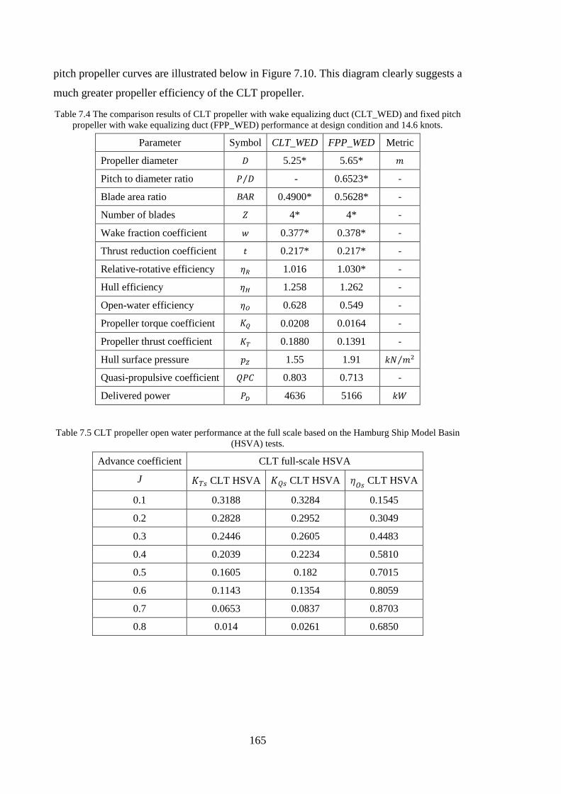
165
pitch propeller curves are illustrated below in Figure 7.10. This diagram clearly suggests a
much greater propeller efficiency of the CLT propeller.
Table 7.4 The comparison results of CLT propeller with wake equalizing duct (CLT_WED) and fixed pitch propeller with wake equalizing duct (FPP_WED) performance at design condition and 14.6 knots.
Parameter Symbol CLT_WED FPP_WED Metric
Propeller diameter 𝐷𝐷 5.25* 5.65* 𝑛𝑛
Pitch to diameter ratio 𝑃𝑃 𝐷𝐷⁄ - 0.6523* -
Blade area ratio BAR 0.4900* 0.5628* -
Number of blades 𝑍𝑍 4* 4* -
Wake fraction coefficient 𝑤𝑤 0.377* 0.378* -
Thrust reduction coefficient 𝐶𝐶 0.217* 0.217* -
Relative-rotative efficiency 𝜂𝜂𝑅𝑅 1.016 1.030* -
Hull efficiency 𝜂𝜂𝐻𝐻 1.258 1.262 -
Open-water efficiency 𝜂𝜂𝑂𝑂 0.628 0.549 -
Propeller torque coefficient 𝐾𝐾𝑄𝑄 0.0208 0.0164 -
Propeller thrust coefficient 𝐾𝐾𝑇𝑇 0.1880 0.1391 -
Hull surface pressure 𝐶𝐶𝑍𝑍 1.55 1.91 𝑘𝑘𝑁𝑁 𝑛𝑛2⁄
Quasi-propulsive coefficient 𝑄𝑄𝑃𝑃𝐶𝐶 0.803 0.713 -
Delivered power 𝑃𝑃𝐷𝐷 4636 5166 𝑘𝑘𝑊𝑊
Table 7.5 CLT propeller open water performance at the full scale based on the Hamburg Ship Model Basin (HSVA) tests.
Advance coefficient CLT full-scale HSVA
J 𝐾𝐾𝑃𝑃𝑔𝑔 CLT HSVA 𝐾𝐾𝑄𝑄𝑔𝑔 CLT HSVA 𝜂𝜂𝐶𝐶𝑔𝑔 CLT HSVA
0.1 0.3188 0.3284 0.1545
0.2 0.2828 0.2952 0.3049
0.3 0.2446 0.2605 0.4483
0.4 0.2039 0.2234 0.5810
0.5 0.1605 0.182 0.7015
0.6 0.1143 0.1354 0.8059
0.7 0.0653 0.0837 0.8703
0.8 0.014 0.0261 0.6850
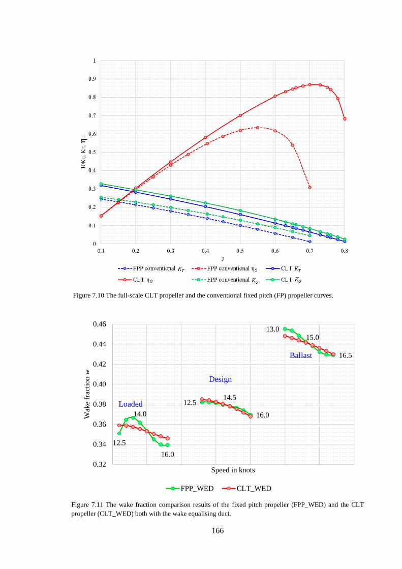
166
Figure 7.10 The full-scale CLT propeller and the conventional fixed pitch (FP) propeller curves.
Figure 7.11 The wake fraction comparison results of the fixed pitch propeller (FPP_WED) and the CLT propeller (CLT_WED) both with the wake equalising duct.
12.5
14.0
16.0
12.514.5
16.0
13.015.0
16.5
0.32
0.34
0.36
0.38
0.40
0.42
0.44
0.46
Wak
e fr
actio
n w
Speed in knots
FPP_WED CLT_WED
Loaded
Design
Ballast
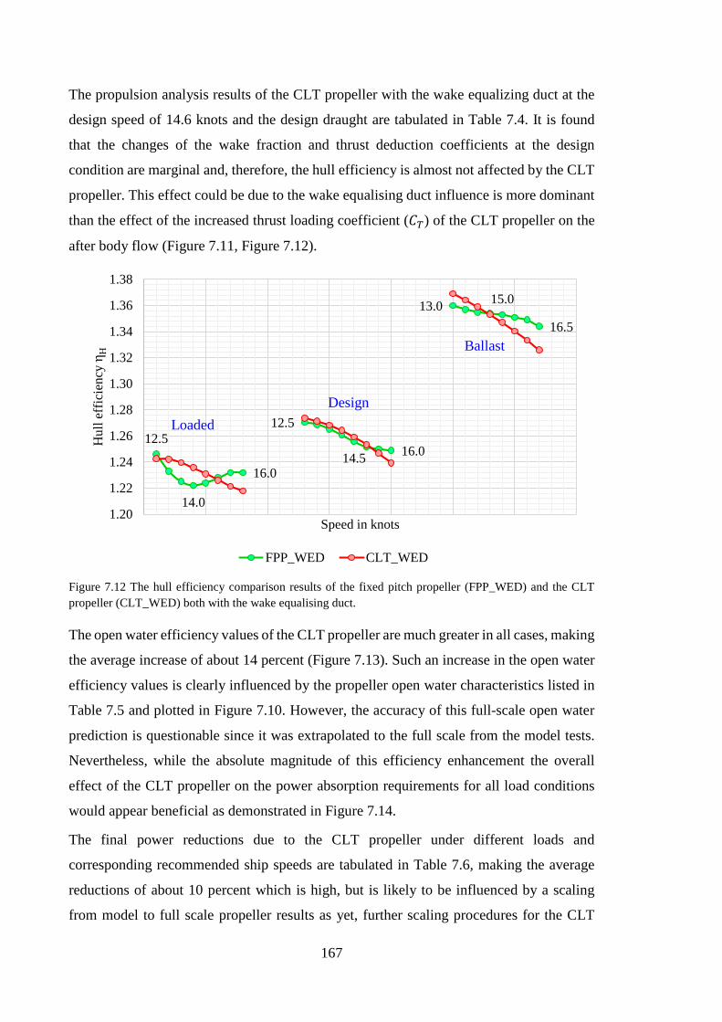
167
The propulsion analysis results of the CLT propeller with the wake equalizing duct at the
design speed of 14.6 knots and the design draught are tabulated in Table 7.4. It is found
that the changes of the wake fraction and thrust deduction coefficients at the design
condition are marginal and, therefore, the hull efficiency is almost not affected by the CLT
propeller. This effect could be due to the wake equalising duct influence is more dominant
than the effect of the increased thrust loading coefficient (𝐶𝐶𝑇𝑇) of the CLT propeller on the
after body flow (Figure 7.11, Figure 7.12).
Figure 7.12 The hull efficiency comparison results of the fixed pitch propeller (FPP_WED) and the CLT propeller (CLT_WED) both with the wake equalising duct.
The open water efficiency values of the CLT propeller are much greater in all cases, making
the average increase of about 14 percent (Figure 7.13). Such an increase in the open water
efficiency values is clearly influenced by the propeller open water characteristics listed in
Table 7.5 and plotted in Figure 7.10. However, the accuracy of this full-scale open water
prediction is questionable since it was extrapolated to the full scale from the model tests.
Nevertheless, while the absolute magnitude of this efficiency enhancement the overall
effect of the CLT propeller on the power absorption requirements for all load conditions
would appear beneficial as demonstrated in Figure 7.14.
The final power reductions due to the CLT propeller under different loads and
corresponding recommended ship speeds are tabulated in Table 7.6, making the average
reductions of about 10 percent which is high, but is likely to be influenced by a scaling
from model to full scale propeller results as yet, further scaling procedures for the CLT
12.5
14.0
16.0
12.5
14.5 16.0
13.0 15.0
16.5
1.20
1.22
1.24
1.26
1.28
1.30
1.32
1.34
1.36
1.38
Hul
l eff
icie
ncy
η H
Speed in knots
FPP_WED CLT_WED
LoadedDesign
Ballast
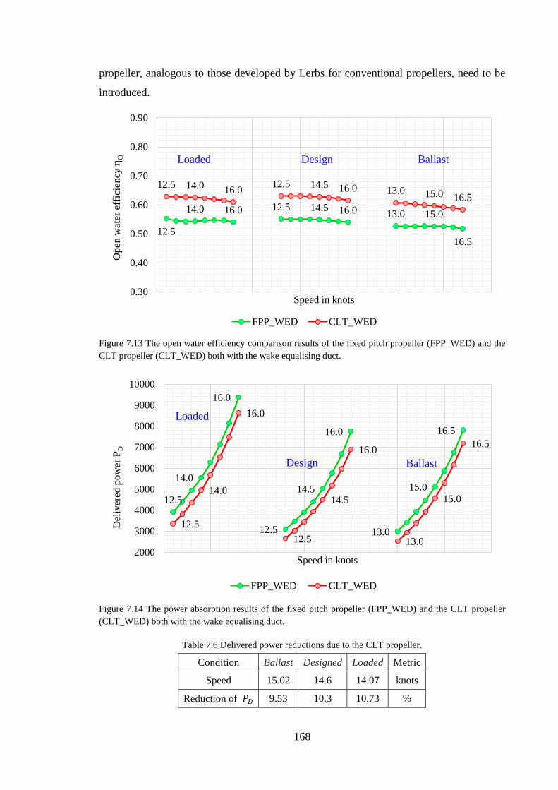
168
propeller, analogous to those developed by Lerbs for conventional propellers, need to be
introduced.
Figure 7.13 The open water efficiency comparison results of the fixed pitch propeller (FPP_WED) and the CLT propeller (CLT_WED) both with the wake equalising duct.
Figure 7.14 The power absorption results of the fixed pitch propeller (FPP_WED) and the CLT propeller (CLT_WED) both with the wake equalising duct.
Table 7.6 Delivered power reductions due to the CLT propeller.
Condition Ballast Designed Loaded Metric
Speed 15.02 14.6 14.07 knots
Reduction of 𝑃𝑃𝐷𝐷 9.53 10.3 10.73 %
12.5
14.0 16.0 12.5 14.5 16.0 13.0 15.0
16.5
12.5 14.0 16.0 12.5 14.5 16.0 13.0 15.0 16.5
0.30
0.40
0.50
0.60
0.70
0.80
0.90O
pen
wat
er e
ffic
ienc
y η O
Speed in knots
FPP_WED CLT_WED
Loaded Design Ballast
12.5
14.0
16.0
12.5
14.5
16.0
13.0
15.0
16.5
12.5
14.0
16.0
12.5
14.5
16.0
13.0
15.0
16.5
2000
3000
4000
5000
6000
7000
8000
9000
10000
Del
iver
ed p
ower
PD
Speed in knots
FPP_WED CLT_WED
BallastDesign
Loaded
169
Ducted Propellers This subsection considers the design and analysis of FP ducted propellers based on the
Wageningen 19A ducted propeller series, fitted with a Ka 4-70 propeller: that is, a four-
bladed propeller having a blade area ratio of 0.70. The 19A duct series uses an accelerating
nozzle combining hydrodynamic advantage with manufacturing ease. This together with
associated ducted propeller series has been applied to the reference medium size products
tanker and further comparison of this propeller performance with the conventional FP
propeller without a nozzle.
The main purpose of an accelerating duct system in this type of application is to enhance
the propeller efficiency by creating an additional thrust stipulated by the circulation induced
around the duct at high thrust loading conditions (Carlton 2012). Alternatively, ducts can
give a negative contribution at low thrust loading conditions due to the skin friction effects
over the duct surface.
In the early 1970s, (Veenman & Zonen 1970) conducted tests with a model of 95,000 DWT
tanker of a conventional hull design and propeller coupled with a range of ducted systems.
Analysis of the reductions in power absorption due to the application of the different ducts
in comparison with the conventional screw propeller was performed for the ship speed of
16.5 knots under loaded and ballast operational conditions. It was found that for both,
loaded and ballast conditions, the most accelerating nozzle provides the largest levels of
power reduction. It was also found that the percentage of delivered power reduction is
generally higher by 2 – 3 percent in the case of ballast condition.
A more recent study by (Koronowicz et al. 2010) is dedicated to the design and analysis of
the ducted propeller performance with the Wageningen 19A nozzle using the computer-
based numerical simulation. The system is claimed to significantly facilitate the process of
design of ducted propellers using the built-in database with a range of the duct geometry
suitable for a wide range of the operating conditions. The comparative analysis has shown
that the ducted propellers may offer competitive performance to open propellers and they
may be successfully applied on ships with high speed.
However, from experience gained in the 1970s where potential efficiency benefits were
predicted from model tests and theoretical modelling, several full-scale comparative trials
were undertaken with tankers and bulk carriers. Full-scale practice did not show that such
prediction was achivable from the analysis of the service data over the course of two years.
Subsequently, the ducts were cut off and the conventional propellers were fitted. The one
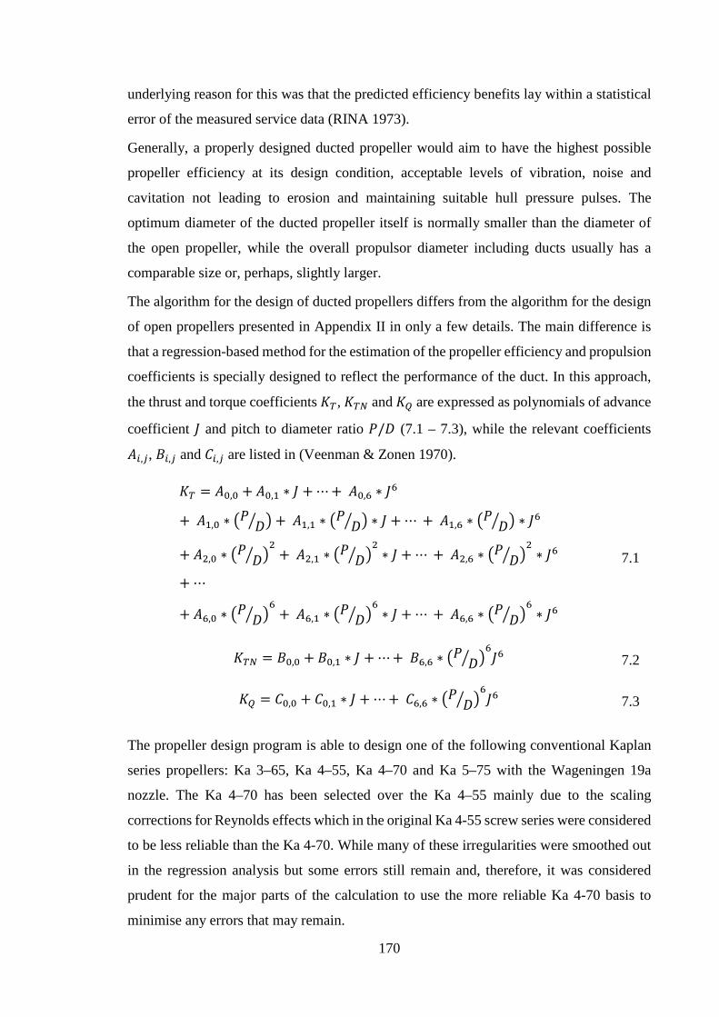
170
underlying reason for this was that the predicted efficiency benefits lay within a statistical
error of the measured service data (RINA 1973).
Generally, a properly designed ducted propeller would aim to have the highest possible
propeller efficiency at its design condition, acceptable levels of vibration, noise and
cavitation not leading to erosion and maintaining suitable hull pressure pulses. The
optimum diameter of the ducted propeller itself is normally smaller than the diameter of
the open propeller, while the overall propulsor diameter including ducts usually has a
comparable size or, perhaps, slightly larger.
The algorithm for the design of ducted propellers differs from the algorithm for the design
of open propellers presented in Appendix II in only a few details. The main difference is
that a regression-based method for the estimation of the propeller efficiency and propulsion
coefficients is specially designed to reflect the performance of the duct. In this approach,
the thrust and torque coefficients 𝐾𝐾𝑇𝑇, 𝐾𝐾𝑇𝑇𝑆𝑆 and 𝐾𝐾𝑄𝑄 are expressed as polynomials of advance
coefficient 𝐽𝐽 and pitch to diameter ratio 𝑃𝑃/𝐷𝐷 (7.1 – 7.3), while the relevant coefficients
𝐵𝐵𝐴𝐴,𝑗𝑗, 𝐵𝐵𝐴𝐴,𝑗𝑗 and 𝐶𝐶𝐴𝐴,𝑗𝑗 are listed in (Veenman & Zonen 1970).
𝐾𝐾𝑇𝑇 = 𝐵𝐵0,0 + 𝐵𝐵0,1 ∗ 𝐽𝐽 + ⋯+ 𝐵𝐵0,6 ∗ 𝐽𝐽6
+ 𝐵𝐵1,0 ∗ 𝑃𝑃 𝐷𝐷 + 𝐵𝐵1,1 ∗ 𝑃𝑃 𝐷𝐷 ∗ 𝐽𝐽 + ⋯ + 𝐵𝐵1,6 ∗ 𝑃𝑃 𝐷𝐷 ∗ 𝐽𝐽6
+ 𝐵𝐵2,0 ∗ 𝑃𝑃 𝐷𝐷 2
+ 𝐵𝐵2,1 ∗ 𝑃𝑃 𝐷𝐷 2∗ 𝐽𝐽 + ⋯ + 𝐵𝐵2,6 ∗ 𝑃𝑃 𝐷𝐷
2∗ 𝐽𝐽6
+ ⋯
+ 𝐵𝐵6,0 ∗ 𝑃𝑃 𝐷𝐷 6
+ 𝐵𝐵6,1 ∗ 𝑃𝑃 𝐷𝐷 6∗ 𝐽𝐽 + ⋯ + 𝐵𝐵6,6 ∗ 𝑃𝑃 𝐷𝐷
6∗ 𝐽𝐽6
7.1
𝐾𝐾𝑇𝑇𝑆𝑆 = 𝐵𝐵0,0 + 𝐵𝐵0,1 ∗ 𝐽𝐽 + ⋯+ 𝐵𝐵6,6 ∗ 𝑃𝑃 𝐷𝐷 6𝐽𝐽6 7.2
𝐾𝐾𝑄𝑄 = 𝐶𝐶0,0 + 𝐶𝐶0,1 ∗ 𝐽𝐽 + ⋯+ 𝐶𝐶6,6 ∗ 𝑃𝑃 𝐷𝐷 6𝐽𝐽6 7.3
The propeller design program is able to design one of the following conventional Kaplan
series propellers: Ka 3–65, Ka 4–55, Ka 4–70 and Ka 5–75 with the Wageningen 19a
nozzle. The Ka 4–70 has been selected over the Ka 4–55 mainly due to the scaling
corrections for Reynolds effects which in the original Ka 4-55 screw series were considered
to be less reliable than the Ka 4-70. While many of these irregularities were smoothed out
in the regression analysis but some errors still remain and, therefore, it was considered
prudent for the major parts of the calculation to use the more reliable Ka 4-70 basis to
minimise any errors that may remain.
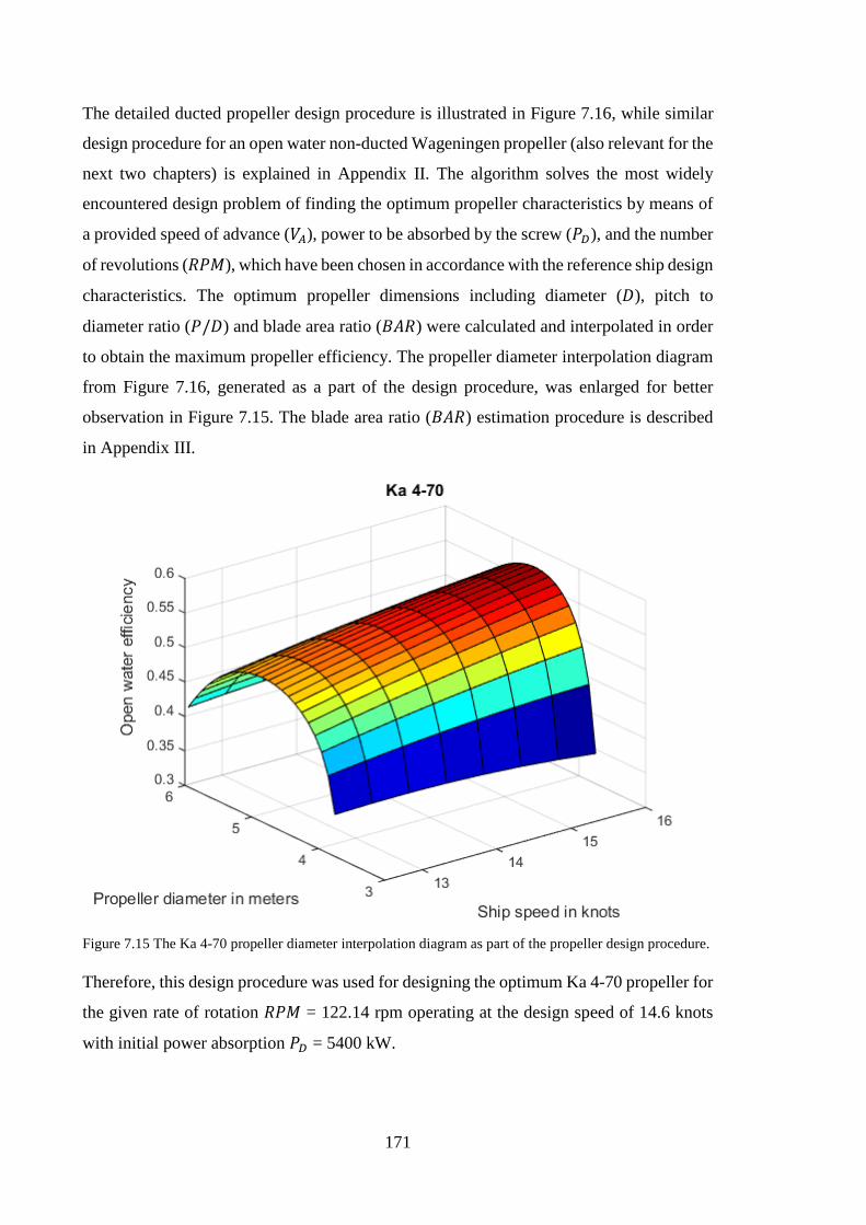
171
The detailed ducted propeller design procedure is illustrated in Figure 7.16, while similar
design procedure for an open water non-ducted Wageningen propeller (also relevant for the
next two chapters) is explained in Appendix II. The algorithm solves the most widely
encountered design problem of finding the optimum propeller characteristics by means of
a provided speed of advance (𝑁𝑁𝐴𝐴), power to be absorbed by the screw (𝑃𝑃𝐷𝐷), and the number
of revolutions (𝐵𝐵𝑃𝑃𝑁𝑁), which have been chosen in accordance with the reference ship design
characteristics. The optimum propeller dimensions including diameter (𝐷𝐷), pitch to
diameter ratio (𝑃𝑃/𝐷𝐷) and blade area ratio (𝐵𝐵𝐵𝐵𝐵𝐵) were calculated and interpolated in order
to obtain the maximum propeller efficiency. The propeller diameter interpolation diagram
from Figure 7.16, generated as a part of the design procedure, was enlarged for better
observation in Figure 7.15. The blade area ratio (𝐵𝐵𝐵𝐵𝐵𝐵) estimation procedure is described
in Appendix III.
Figure 7.15 The Ka 4-70 propeller diameter interpolation diagram as part of the propeller design procedure.
Therefore, this design procedure was used for designing the optimum Ka 4-70 propeller for
the given rate of rotation 𝐵𝐵𝑃𝑃𝑁𝑁 = 122.14 rpm operating at the design speed of 14.6 knots
with initial power absorption 𝑃𝑃𝐷𝐷 = 5400 kW.
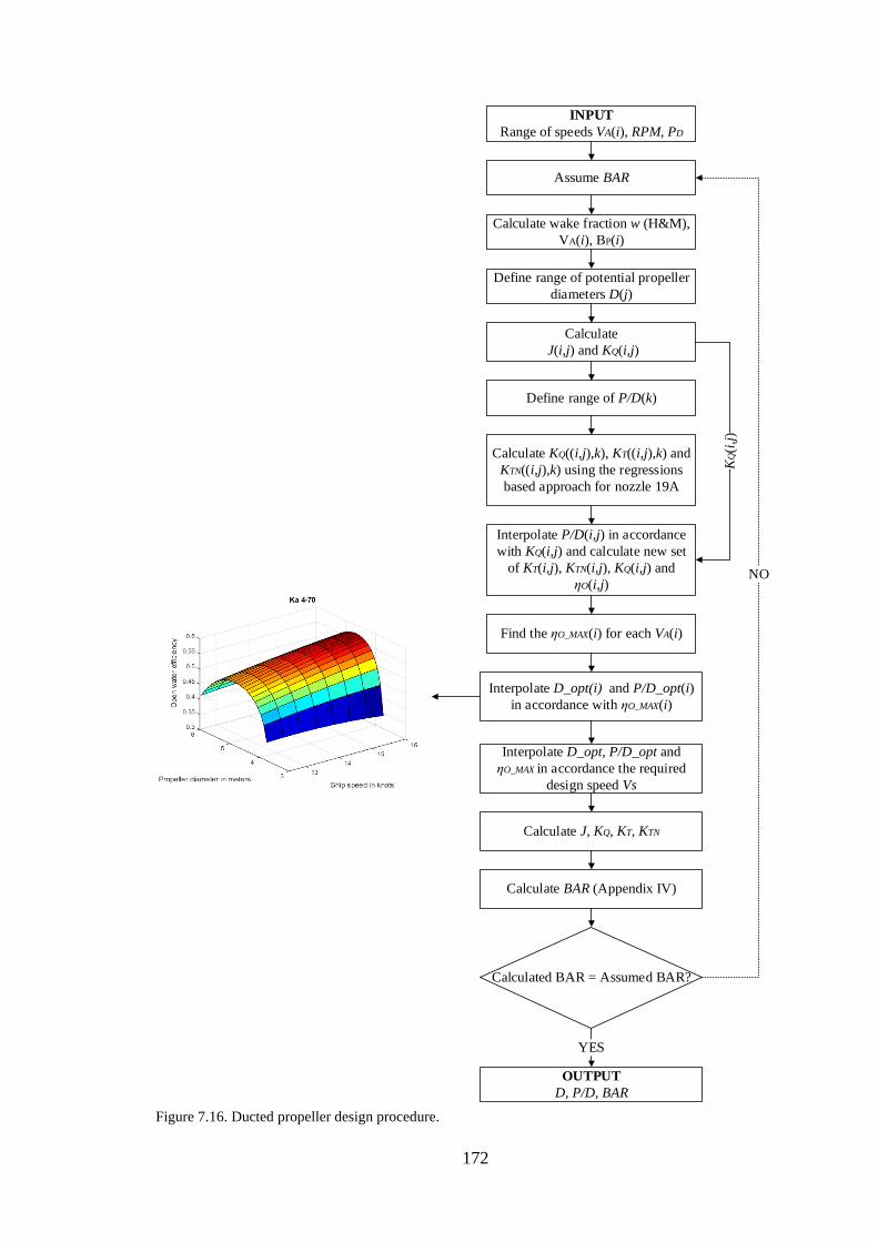
172
INPUTRange of speeds VA(i), RPM, PD
Calculate wake fraction w (H&M),VA(i), BP(i)
Calculate J(i,j) and KQ(i,j)
Define range of potential propeller diameters D(j)
Assume BAR
Define range of P/D(k)
Calculate KQ((i,j),k), KT((i,j),k) and KTN((i,j),k) using the regressions based approach for nozzle 19A
Interpolate P/D(i,j) in accordance with KQ(i,j) and calculate new set
of KT(i,j), KTN(i,j), KQ(i,j) and ηO(i,j)
KQ(i,
j)
Find the ηO_MAX(i) for each VA(i)
Interpolate D_opt(i) and P/D_opt(i) in accordance with ηO_MAX(i)
Interpolate D_opt, P/D_opt and ηO_MAX in accordance the required
design speed Vs
Calculate J, KQ, KT, KTN
Calculate BAR (Appendix IV)
Calculated BAR = Assumed BAR?
NO
OUTPUT D, P/D, BAR
YES
Figure 7.16. Ducted propeller design procedure.
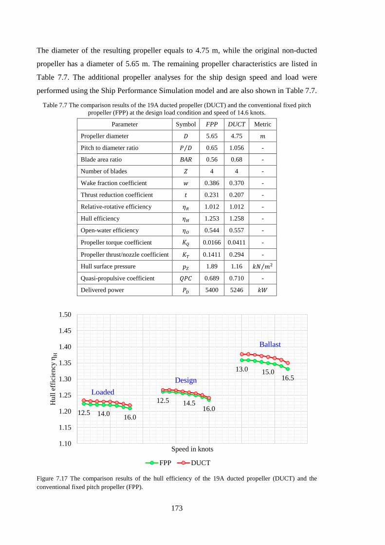
173
The diameter of the resulting propeller equals to 4.75 m, while the original non-ducted
propeller has a diameter of 5.65 m. The remaining propeller characteristics are listed in
Table 7.7. The additional propeller analyses for the ship design speed and load were
performed using the Ship Performance Simulation model and are also shown in Table 7.7.
Table 7.7 The comparison results of the 19A ducted propeller (DUCT) and the conventional fixed pitch propeller (FPP) at the design load condition and speed of 14.6 knots.
Parameter Symbol FPP DUCT Metric
Propeller diameter 𝐷𝐷 5.65 4.75 𝑛𝑛
Pitch to diameter ratio 𝑃𝑃 𝐷𝐷⁄ 0.65 1.056 -
Blade area ratio BAR 0.56 0.68 -
Number of blades 𝑍𝑍 4 4 -
Wake fraction coefficient 𝑤𝑤 0.386 0.370 -
Thrust reduction coefficient 𝐶𝐶 0.231 0.207 -
Relative-rotative efficiency 𝜂𝜂𝑅𝑅 1.012 1.012 -
Hull efficiency 𝜂𝜂𝐻𝐻 1.253 1.258 -
Open-water efficiency 𝜂𝜂𝑂𝑂 0.544 0.557 -
Propeller torque coefficient 𝐾𝐾𝑄𝑄 0.0166 0.0411 -
Propeller thrust/nozzle coefficient 𝐾𝐾𝑇𝑇 0.1411 0.294 -
Hull surface pressure 𝐶𝐶𝑍𝑍 1.89 1.16 𝑘𝑘𝑁𝑁 𝑛𝑛2⁄
Quasi-propulsive coefficient 𝑄𝑄𝑃𝑃𝐶𝐶 0.689 0.710 -
Delivered power 𝑃𝑃𝐷𝐷 5400 5246 𝑘𝑘𝑊𝑊
Figure 7.17 The comparison results of the hull efficiency of the 19A ducted propeller (DUCT) and the conventional fixed pitch propeller (FPP).
12.5 14.0 16.0
12.5 14.516.0
13.0 15.016.5
1.10
1.15
1.20
1.25
1.30
1.35
1.40
1.45
1.50
Hul
l eff
icie
ncy
η H
Speed in knots
FPP DUCT
LoadedDesign
Ballast
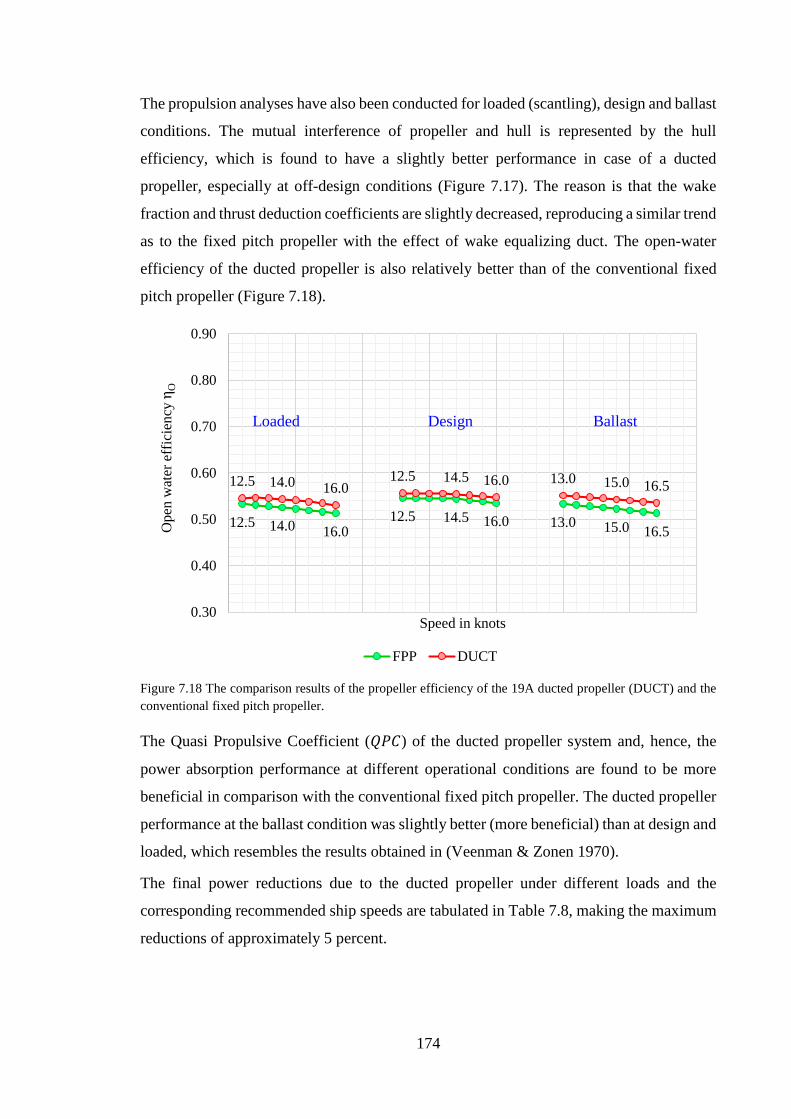
174
The propulsion analyses have also been conducted for loaded (scantling), design and ballast
conditions. The mutual interference of propeller and hull is represented by the hull
efficiency, which is found to have a slightly better performance in case of a ducted
propeller, especially at off-design conditions (Figure 7.17). The reason is that the wake
fraction and thrust deduction coefficients are slightly decreased, reproducing a similar trend
as to the fixed pitch propeller with the effect of wake equalizing duct. The open-water
efficiency of the ducted propeller is also relatively better than of the conventional fixed
pitch propeller (Figure 7.18).
Figure 7.18 The comparison results of the propeller efficiency of the 19A ducted propeller (DUCT) and the conventional fixed pitch propeller.
The Quasi Propulsive Coefficient (𝑄𝑄𝑃𝑃𝐶𝐶) of the ducted propeller system and, hence, the
power absorption performance at different operational conditions are found to be more
beneficial in comparison with the conventional fixed pitch propeller. The ducted propeller
performance at the ballast condition was slightly better (more beneficial) than at design and
loaded, which resembles the results obtained in (Veenman & Zonen 1970).
The final power reductions due to the ducted propeller under different loads and the
corresponding recommended ship speeds are tabulated in Table 7.8, making the maximum
reductions of approximately 5 percent.
12.5 14.0 16.012.5 14.5 16.0 13.0 15.0 16.5
12.5 14.0 16.012.5 14.5 16.0 13.0 15.0 16.5
0.30
0.40
0.50
0.60
0.70
0.80
0.90
Ope
n w
ater
eff
icie
ncy
η O
Speed in knots
FPP DUCT
Loaded Design Ballast
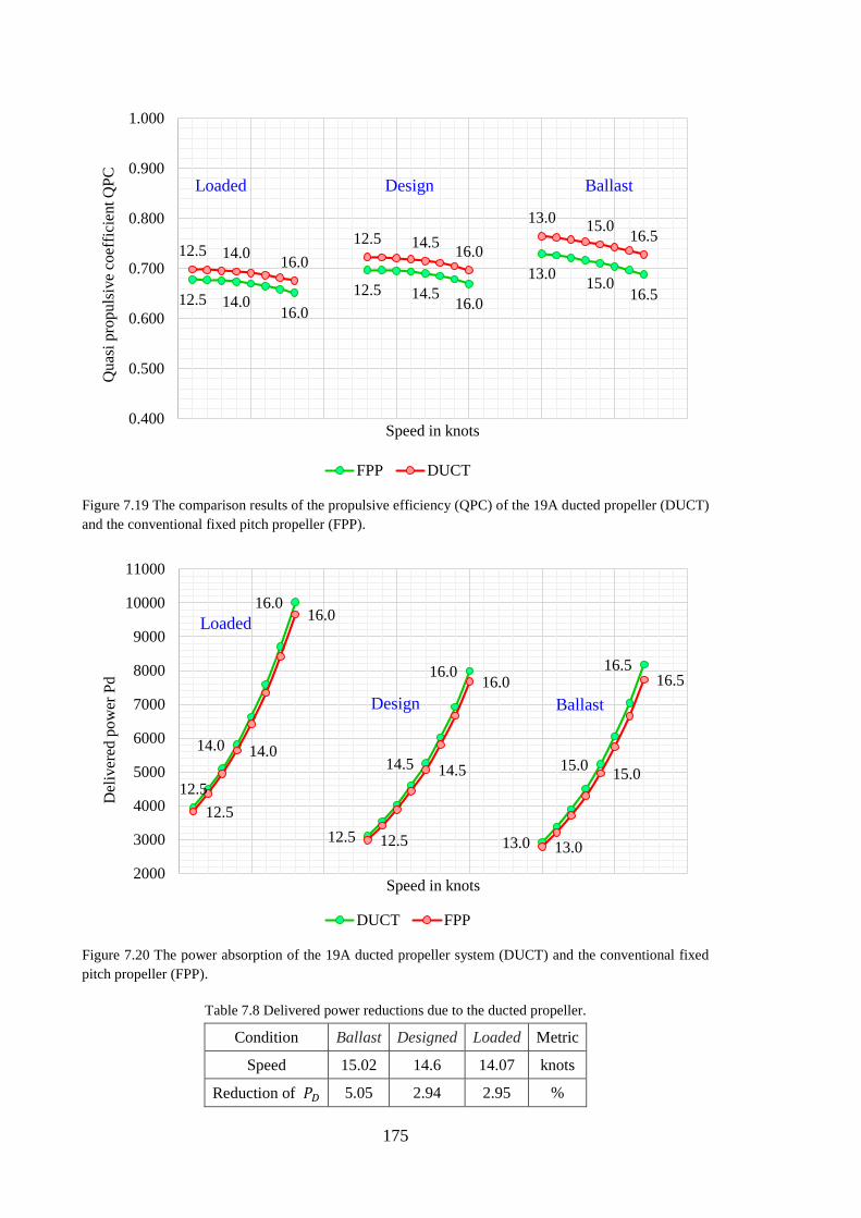
175
Figure 7.19 The comparison results of the propulsive efficiency (QPC) of the 19A ducted propeller (DUCT) and the conventional fixed pitch propeller (FPP).
Figure 7.20 The power absorption of the 19A ducted propeller system (DUCT) and the conventional fixed pitch propeller (FPP).
Table 7.8 Delivered power reductions due to the ducted propeller.
Condition Ballast Designed Loaded Metric
Speed 15.02 14.6 14.07 knots
Reduction of 𝑃𝑃𝐷𝐷 5.05 2.94 2.95 %
12.5 14.016.0
12.5 14.5 16.0
13.0 15.016.5
12.5 14.0 16.012.5 14.5 16.0
13.0 15.0 16.5
0.400
0.500
0.600
0.700
0.800
0.900
1.000Q
uasi
pro
puls
ive
coef
ficie
nt Q
PC
Speed in knots
FPP DUCT
BallastDesignLoaded
12.5
14.0
16.0
12.5
14.5
16.0
13.0
15.0
16.5
12.5
14.0
16.0
12.5
14.5
16.0
13.0
15.0
16.5
2000
3000
4000
5000
6000
7000
8000
9000
10000
11000
Del
iver
ed p
ower
Pd
Speed in knots
DUCT FPP
BallastDesign
Loaded
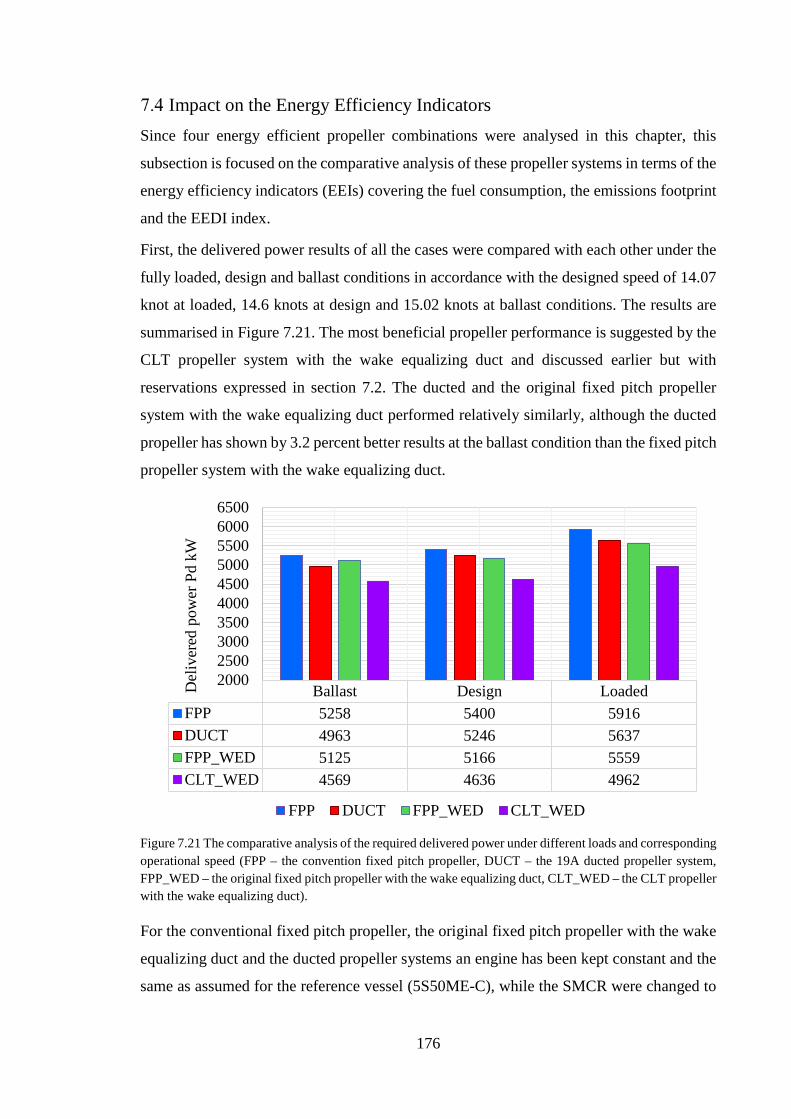
176
Impact on the Energy Efficiency Indicators Since four energy efficient propeller combinations were analysed in this chapter, this
subsection is focused on the comparative analysis of these propeller systems in terms of the
energy efficiency indicators (EEIs) covering the fuel consumption, the emissions footprint
and the EEDI index.
First, the delivered power results of all the cases were compared with each other under the
fully loaded, design and ballast conditions in accordance with the designed speed of 14.07
knot at loaded, 14.6 knots at design and 15.02 knots at ballast conditions. The results are
summarised in Figure 7.21. The most beneficial propeller performance is suggested by the
CLT propeller system with the wake equalizing duct and discussed earlier but with
reservations expressed in section 7.2. The ducted and the original fixed pitch propeller
system with the wake equalizing duct performed relatively similarly, although the ducted
propeller has shown by 3.2 percent better results at the ballast condition than the fixed pitch
propeller system with the wake equalizing duct.
Figure 7.21 The comparative analysis of the required delivered power under different loads and corresponding operational speed (FPP – the convention fixed pitch propeller, DUCT – the 19A ducted propeller system, FPP_WED – the original fixed pitch propeller with the wake equalizing duct, CLT_WED – the CLT propeller with the wake equalizing duct).
For the conventional fixed pitch propeller, the original fixed pitch propeller with the wake
equalizing duct and the ducted propeller systems an engine has been kept constant and the
same as assumed for the reference vessel (5S50ME-C), while the SMCR were changed to
Ballast Design LoadedFPP 5258 5400 5916DUCT 4963 5246 5637FPP_WED 5125 5166 5559CLT_WED 4569 4636 4962
2000250030003500400045005000550060006500
Del
iver
ed p
ower
Pd
kW
FPP DUCT FPP_WED CLT_WED
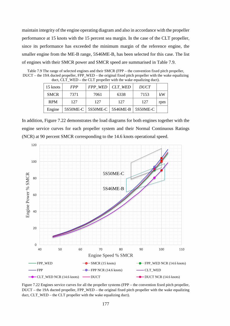
177
maintain integrity of the engine operating diagram and also in accordance with the propeller
performance at 15 knots with the 15 percent sea margin. In the case of the CLT propeller,
since its performance has exceeded the minimum margin of the reference engine, the
smaller engine from the ME-B range, 5S46ME-B, has been selected for this case. The list
of engines with their SMCR power and SMCR speed are summarised in Table 7.9.
Table 7.9 The range of selected engines and their SMCR (FPP – the convention fixed pitch propeller, DUCT – the 19A ducted propeller, FPP_WED – the original fixed pitch propeller with the wake equalizing
duct, CLT_WED – the CLT propeller with the wake equalizing duct).
15 knots FPP FPP_WED CLT_WED DUCT
SMCR 7371 7061 6338 7153 kW
RPM 127 127 127 127 rpm
Engine 5S50ME-C 5S50ME-C 5S46ME-B 5S50ME-C
In addition, Figure 7.22 demonstrates the load diagrams for both engines together with the
engine service curves for each propeller system and their Normal Continuous Ratings
(NCR) at 90 percent SMCR corresponding to the 14.6 knots operational speed.
Figure 7.22 Engines service curves for all the propeller systems (FPP – the convention fixed pitch propeller, DUCT – the 19A ducted propeller, FPP_WED – the original fixed pitch propeller with the wake equalizing duct, CLT_WED – the CLT propeller with the wake equalizing duct).
0
20
40
60
80
100
120
40 50 60 70 80 90 100 110
Engi
ne P
ower
% S
MC
R
Engine Speed % SMCRFPP_WED SMCR (15 knots) FPP_WED NCR (14.6 knots)
FPP FPP NCR (14.6 knots) CLT_WED
CLT_WED NCR (14.6 knots) DUCT DUCT NCR (14.6 knots)
5S50ME-C
5S46ME-B
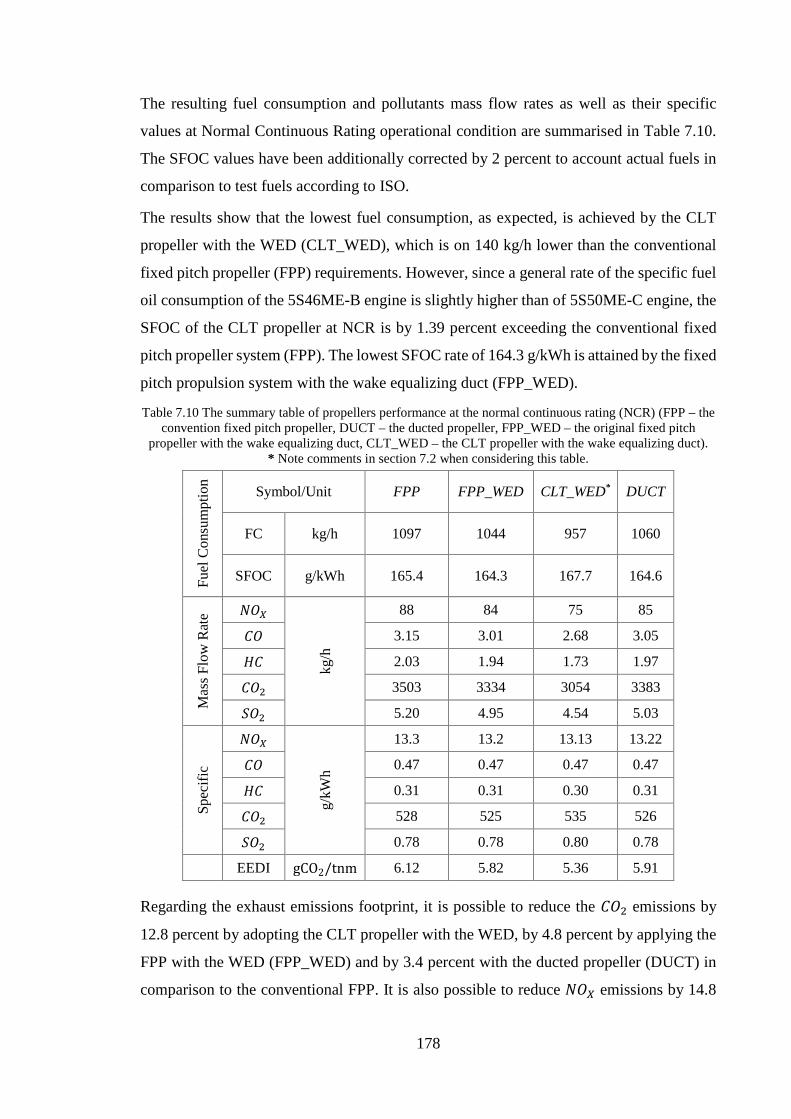
178
The resulting fuel consumption and pollutants mass flow rates as well as their specific
values at Normal Continuous Rating operational condition are summarised in Table 7.10.
The SFOC values have been additionally corrected by 2 percent to account actual fuels in
comparison to test fuels according to ISO.
The results show that the lowest fuel consumption, as expected, is achieved by the CLT
propeller with the WED (CLT_WED), which is on 140 kg/h lower than the conventional
fixed pitch propeller (FPP) requirements. However, since a general rate of the specific fuel
oil consumption of the 5S46ME-B engine is slightly higher than of 5S50ME-C engine, the
SFOC of the CLT propeller at NCR is by 1.39 percent exceeding the conventional fixed
pitch propeller system (FPP). The lowest SFOC rate of 164.3 g/kWh is attained by the fixed
pitch propulsion system with the wake equalizing duct (FPP_WED).
Table 7.10 The summary table of propellers performance at the normal continuous rating (NCR) (FPP – the convention fixed pitch propeller, DUCT – the ducted propeller, FPP_WED – the original fixed pitch
propeller with the wake equalizing duct, CLT_WED – the CLT propeller with the wake equalizing duct). * Note comments in section 7.2 when considering this table.
Fuel
Con
sum
ptio
n
Symbol/Unit FPP FPP_WED CLT_WED* DUCT
FC kg/h 1097 1044 957 1060
SFOC g/kWh 165.4 164.3 167.7 164.6
Mas
s Flo
w R
ate 𝑁𝑁𝐶𝐶𝑋𝑋
kg/h
88 84 75 85
𝐶𝐶𝐶𝐶 3.15 3.01 2.68 3.05
𝐻𝐻𝐶𝐶 2.03 1.94 1.73 1.97
𝐶𝐶𝐶𝐶2 3503 3334 3054 3383
𝑆𝑆𝐶𝐶2 5.20 4.95 4.54 5.03
Spec
ific
𝑁𝑁𝐶𝐶𝑋𝑋
g/kW
h
13.3 13.2 13.13 13.22
𝐶𝐶𝐶𝐶 0.47 0.47 0.47 0.47
𝐻𝐻𝐶𝐶 0.31 0.31 0.30 0.31
𝐶𝐶𝐶𝐶2 528 525 535 526
𝑆𝑆𝐶𝐶2 0.78 0.78 0.80 0.78
EEDI gCO2/tnm 6.12 5.82 5.36 5.91
Regarding the exhaust emissions footprint, it is possible to reduce the 𝐶𝐶𝐶𝐶2 emissions by
12.8 percent by adopting the CLT propeller with the WED, by 4.8 percent by applying the
FPP with the WED (FPP_WED) and by 3.4 percent with the ducted propeller (DUCT) in
comparison to the conventional FPP. It is also possible to reduce 𝑁𝑁𝐶𝐶𝑋𝑋 emissions by 14.8
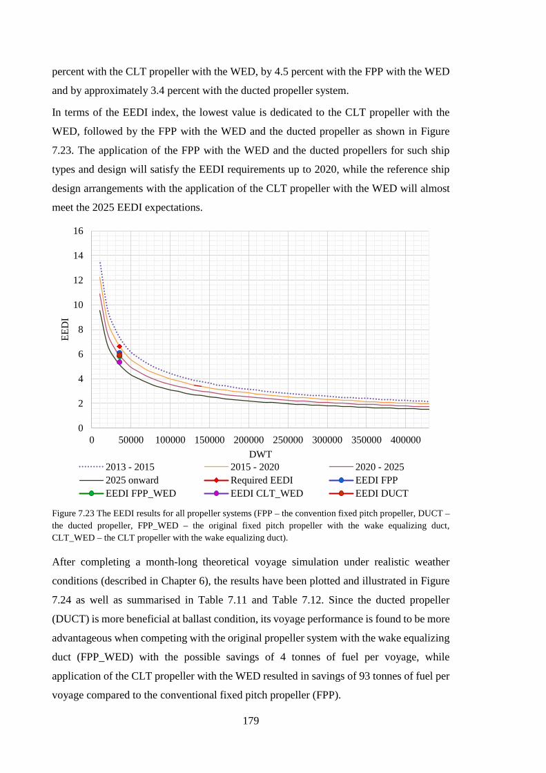
179
percent with the CLT propeller with the WED, by 4.5 percent with the FPP with the WED
and by approximately 3.4 percent with the ducted propeller system.
In terms of the EEDI index, the lowest value is dedicated to the CLT propeller with the
WED, followed by the FPP with the WED and the ducted propeller as shown in Figure
7.23. The application of the FPP with the WED and the ducted propellers for such ship
types and design will satisfy the EEDI requirements up to 2020, while the reference ship
design arrangements with the application of the CLT propeller with the WED will almost
meet the 2025 EEDI expectations.
Figure 7.23 The EEDI results for all propeller systems (FPP – the convention fixed pitch propeller, DUCT – the ducted propeller, FPP_WED – the original fixed pitch propeller with the wake equalizing duct, CLT_WED – the CLT propeller with the wake equalizing duct).
After completing a month-long theoretical voyage simulation under realistic weather
conditions (described in Chapter 6), the results have been plotted and illustrated in Figure
7.24 as well as summarised in Table 7.11 and Table 7.12. Since the ducted propeller
(DUCT) is more beneficial at ballast condition, its voyage performance is found to be more
advantageous when competing with the original propeller system with the wake equalizing
duct (FPP_WED) with the possible savings of 4 tonnes of fuel per voyage, while
application of the CLT propeller with the WED resulted in savings of 93 tonnes of fuel per
voyage compared to the conventional fixed pitch propeller (FPP).
0
2
4
6
8
10
12
14
16
0 50000 100000 150000 200000 250000 300000 350000 400000
EED
I
DWT2013 - 2015 2015 - 2020 2020 - 20252025 onward Required EEDI EEDI FPPEEDI FPP_WED EEDI CLT_WED EEDI DUCT
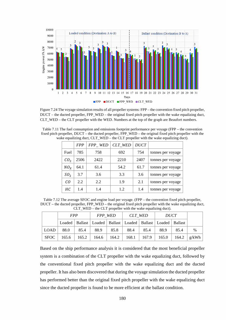
180
Figure 7.24 The voyage simulation results of all propeller systems: FPP – the convention fixed pitch propeller, DUCT – the ducted propeller, FPP_WED – the original fixed pitch propeller with the wake equalizing duct, CLT_WED – the CLT propeller with the WED. Numbers at the top of the graph are Beaufort numbers.
Table 7.11 The fuel consumption and emissions footprint performance per voyage (FPP – the convention fixed pitch propeller, DUCT – the ducted propeller, FPP_WED – the original fixed pitch propeller with the
wake equalizing duct, CLT_WED – the CLT propeller with the wake equalizing duct).
FPP FPP_ WED CLT_WED DUCT
Fuel 785 758 692 754 tonnes per voyage
𝐶𝐶𝐶𝐶2 2506 2422 2210 2407 tonnes per voyage
𝑁𝑁𝐶𝐶𝑋𝑋 64.1 61.4 54.2 61.7 tonnes per voyage
𝑆𝑆𝐶𝐶2 3.7 3.6 3.3 3.6 tonnes per voyage
𝐶𝐶𝐶𝐶 2.2 2.2 1.9 2.1 tonnes per voyage
𝐻𝐻𝐶𝐶 1.4 1.4 1.2 1.4 tonnes per voyage
Table 7.12 The average SFOC and engine load per voyage. (FPP – the convention fixed pitch propeller, DUCT – the ducted propeller, FPP_WED – the original fixed pitch propeller with the wake equalizing duct,
CLT_WED – the CLT propeller with the wake equalizing duct).
FPP FPP_WED CLT_WED DUCT
Loaded Ballast Loaded Ballast Loaded Ballast Loaded Ballast
LOAD 88.0 85.4 88.9 85.8 88.4 85.4 88.9 85.4 %
SFOC 165.6 165.2 164.6 164.2 168.1 167.9 165.0 164.2 g/kWh
Based on the ship performance analysis it is considered that the most beneficial propeller
system is a combination of the CLT propeller with the wake equalizing duct, followed by
the conventional fixed pitch propeller with the wake equalizing duct and the ducted
propeller. It has also been discovered that during the voyage simulation the ducted propeller
has performed better than the original fixed pitch propeller with the wake equalizing duct
since the ducted propeller is found to be more efficient at the ballast condition.
181
8 Propeller Optimisation
Besides the energy efficient propeller designs, examined in the previous chapter, there are
also a number of propeller design characteristics that can be further optimised to potentially
provide a positive impact on the overall propulsion efficiency. Namely, propulsion
efficiency improvements may be achieved by increasing the propeller diameter or
decreasing the blade area ratio (or both). However, the scale of changes is restricted by the
hull dimensions and the level of generated hull surface pressure pulses, in the case of an
artificially increased propeller diameter, while governed by cavitation avoidance margins
when decreasing the propeller blade area ratio.
The cavitation phenomenon occurs when the local fluid pressure drops to the vapour
pressure level or below causing the formation of cavities. When these cavitation structures
collapse, mostly in times considerably less that one second, this gives rise to significant
pressure fluctuations induced by a variety of collapse mechanisms. The presence of
cavitation disturbs the flow around the propeller surface, which can in extreme cases
negatively affect the propulsion characteristics, namely, give rise to deteriorations in thrust
and torque performance resulting in the reduction of the propulsion efficiency and,
potentially, in erosion on the propeller blade surface due to the collapsing cavitation
bubbles (Molland et al. 2011). In addition, hydrodynamic pressure fluctuations, also caused
by the cavitation bubbles, may result in an unacceptable level of noise and vibration in the
ship.
To limit the harmful effects of cavitation, it is important to carefully select the blade area
ratio ensuring that the global thrust loading, in other words, the ratio of the delivered thrust
to the total blade area of the propeller, lies within the acceptable cavitation limits. The
cavitation limits are normally estimated for each propeller case individually during the
detailed design stage by applying the Gutsche or Walcher “bucket” type diagrams or by
implementing cavitation tunnel tests and detailed flow analysis.
For the preliminary cavitation predictions as well as for the calculation of a suitable 𝐵𝐵𝐵𝐵𝐵𝐵,
as already mentioned in Chapter 2.3, there are two widely used empirical methods, namely,
those derived by Burrill and Keller. Both the Burrill and Keller methods have been
extensively used by propeller designers for preliminary estimations of the required 𝐵𝐵𝐵𝐵𝐵𝐵 to
avoid excessive cavitation (Carlton 2012), while according to (Trodden & Woodward
2013), the Burrill’s method has shown more conservative results than the Keller’s formula.
It is important to emphasize that according to the Burrill’s method an acceptable upper limit

182
of back cavitation for merchant vessels is in the region of 5 percent, while the thrust
breakdown does not usually occur before approximately 20 percent back cavitation has
been developed. The actual level of the breakdown limit is a matter for the propeller
designer in terms of the ship's operational profile.
In case a smaller 𝐵𝐵𝐵𝐵𝐵𝐵 is desired, the control of cavitation appearance may also be achieved
by increasing the propeller diameter, which helps to distribute the excessive thrust loading
across the propeller disk while smoothing out the fluctuating pressure peaks. In addition,
as already outlined above, the application of bigger propeller diameters is more
hydrodynamically efficient. However, there are certain constraints and rules that have to
be observed when increasing the propeller diameter artificially, while keeping the rotational
speed constant.
The first one is to keep sufficient clearances between the propeller and the hull, which are
important to minimise the risk of on-board noise and vibration. Secondly, a larger propeller
diameter could give rise to the wake fluctuations causing the reduction in hull efficiency
due to a decrease in the average value of the wake fraction (Ghose & Gokarn 2009). It is
also important to take into account the propeller and the hull interactions, namely hull
surface pressure pulses being transmitted from the propeller through the water and also the
global system of forces and moments transmitted through the bearing system to the hull.
The hull surface pressure depends upon the ship type, shape of the stern and the propeller
size.
In summary, the reduction of the propeller blade area ratio will most likely result in
improvements of the propeller performance in terms of energy efficiency, while also may
increase the risk of cavitation and attendant erosion. However, from the current research
and development in this area, we see a rising interest from the industry to minimise the
damage from the cavitation phenomenon not only by implementing cavitation safe
propeller designs but also by finding innovative composite materials or coatings with robust
anti-cavitation properties.
For example, in (Yamatogi et al. 2009) the authors have examined the cavitation erosion
resistance of the Aramid Fibre Reinforced Polymer (AFRP) and found that the fibrils
covered over the surface tend to absorb the impact of impulses during the cavitation
collapse making it difficult for erosion to progress. Other work done by (Bregliozzi et al.
2005) is focused on the examination of the cavitation erosion behaviour of AISI 304 steel
and high nitrogen containing austenitic stainless steel as a function of the grain size. It has
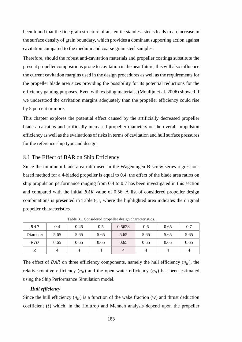
183
been found that the fine grain structure of austenitic stainless steels leads to an increase in
the surface density of grain boundary, which provides a dominant supporting action against
cavitation compared to the medium and coarse grain steel samples.
Therefore, should the robust anti-cavitation materials and propeller coatings substitute the
present propeller compositions prone to cavitation in the near future, this will also influence
the current cavitation margins used in the design procedures as well as the requirements for
the propeller blade area sizes providing the possibility for its potential reductions for the
efficiency gaining purposes. Even with existing materials, (Moulijn et al. 2006) showed if
we understood the cavitation margins adequately than the propeller efficiency could rise
by 5 percent or more.
This chapter explores the potential effect caused by the artificially decreased propeller
blade area ratios and artificially increased propeller diameters on the overall propulsion
efficiency as well as the evaluations of risks in terms of cavitation and hull surface pressures
for the reference ship type and design.
The Effect of BAR on Ship Efficiency Since the minimum blade area ratio used in the Wageningen B-screw series regression-
based method for a 4-bladed propeller is equal to 0.4, the effect of the blade area ratios on
ship propulsion performance ranging from 0.4 to 0.7 has been investigated in this section
and compared with the initial 𝐵𝐵𝐵𝐵𝐵𝐵 value of 0.56. A list of considered propeller design
combinations is presented in Table 8.1, where the highlighted area indicates the original
propeller characteristics.
Table 8.1 Considered propeller design characteristics.
𝐵𝐵𝐵𝐵𝐵𝐵 0.4 0.45 0.5 0.5628 0.6 0.65 0.7
Diameter 5.65 5.65 5.65 5.65 5.65 5.65 5.65
𝑃𝑃/𝐷𝐷 0.65 0.65 0.65 0.65 0.65 0.65 0.65
𝑍𝑍 4 4 4 4 4 4 4
The effect of 𝐵𝐵𝐵𝐵𝐵𝐵 on three efficiency components, namely the hull efficiency (𝜂𝜂𝐻𝐻), the
relative-rotative efficiency (𝜂𝜂𝑅𝑅) and the open water efficiency (𝜂𝜂𝑂𝑂) has been estimated
using the Ship Performance Simulation model.
Hull efficiency
Since the hull efficiency (𝜂𝜂𝐻𝐻) is a function of the wake fraction (𝑤𝑤) and thrust deduction
coefficient (𝐶𝐶) which, in the Holttrop and Mennen analysis depend upon the propeller
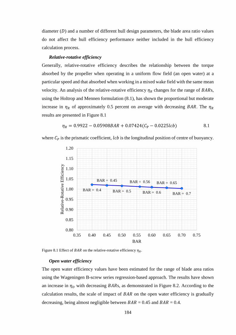
184
diameter (𝐷𝐷) and a number of different hull design parameters, the blade area ratio values
do not affect the hull efficiency performance neither included in the hull efficiency
calculation process.
Relative-rotative efficiency
Generally, relative-rotative efficiency describes the relationship between the torque
absorbed by the propeller when operating in a uniform flow field (an open water) at a
particular speed and that absorbed when working in a mixed wake field with the same mean
velocity. An analysis of the relative-rotative efficiency 𝜂𝜂𝑅𝑅 changes for the range of 𝐵𝐵𝐵𝐵𝐵𝐵s,
using the Holtrop and Mennen formulation (8.1), has shown the proportional but moderate
increase in 𝜂𝜂𝑅𝑅 of approximately 0.5 percent on average with decreasing 𝐵𝐵𝐵𝐵𝐵𝐵. The 𝜂𝜂𝑅𝑅
results are presented in Figure 8.1
𝜂𝜂𝑅𝑅 = 0.9922 − 0.05908𝐵𝐵𝐵𝐵𝐵𝐵 + 0.07424(𝐶𝐶P − 0.0225𝑙𝑙𝐶𝐶𝑙𝑙) 8.1
where 𝐶𝐶𝑃𝑃 is the prismatic coefficient, 𝑙𝑙𝐶𝐶𝑙𝑙 is the longitudinal position of centre of buoyancy.
Figure 8.1 Effect of 𝐵𝐵𝐵𝐵𝐵𝐵 on the relative-rotative efficiency 𝜂𝜂𝑅𝑅.
Open water efficiency
The open water efficiency values have been estimated for the range of blade area ratios
using the Wageningen B-screw series regression-based approach. The results have shown
an increase in 𝜂𝜂𝑂𝑂 with decreasing 𝐵𝐵𝐵𝐵𝐵𝐵s, as demonstrated in Figure 8.2. According to the
calculation results, the scale of impact of 𝐵𝐵𝐵𝐵𝐵𝐵 on the open water efficiency is gradually
decreasing, being almost negligible between 𝐵𝐵𝐵𝐵𝐵𝐵 = 0.45 and 𝐵𝐵𝐵𝐵𝐵𝐵 = 0.4.
BAR = 0.4
BAR = 0.45
BAR = 0.5
BAR = 0.56
BAR = 0.6
BAR = 0.65
BAR = 0.7
0.80
0.85
0.90
0.95
1.00
1.05
1.10
1.15
1.20
0.35 0.40 0.45 0.50 0.55 0.60 0.65 0.70 0.75
Rel
ativ
e-R
otat
ive
Effic
ienc
y
BAR
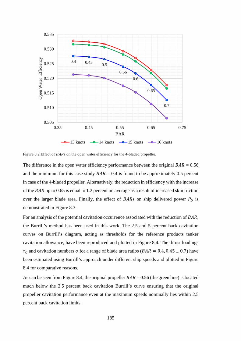
185
Figure 8.2 Effect of 𝐵𝐵𝐵𝐵𝐵𝐵s on the open water efficiency for the 4-bladed propeller.
The difference in the open water efficiency performance between the original 𝐵𝐵𝐵𝐵𝐵𝐵 = 0.56
and the minimum for this case study 𝐵𝐵𝐵𝐵𝐵𝐵 = 0.4 is found to be approximately 0.5 percent
in case of the 4-bladed propeller. Alternatively, the reduction in efficiency with the increase
of the 𝐵𝐵𝐵𝐵𝐵𝐵 up to 0.65 is equal to 1.2 percent on average as a result of increased skin friction
over the larger blade area. Finally, the effect of 𝐵𝐵𝐵𝐵𝐵𝐵s on ship delivered power 𝑃𝑃𝐷𝐷 is
demonstrated in Figure 8.3.
For an analysis of the potential cavitation occurrence associated with the reduction of 𝐵𝐵𝐵𝐵𝐵𝐵,
the Burrill’s method has been used in this work. The 2.5 and 5 percent back cavitation
curves on Burrill’s diagram, acting as thresholds for the reference products tanker
cavitation allowance, have been reproduced and plotted in Figure 8.4. The thrust loadings
𝜏𝜏𝐶𝐶 and cavitation numbers 𝜎𝜎 for a range of blade area ratios (𝐵𝐵𝐵𝐵𝐵𝐵 = 0.4, 0.45 … 0.7) have
been estimated using Burrill’s approach under different ship speeds and plotted in Figure
8.4 for comparative reasons.
As can be seen from Figure 8.4, the original propeller 𝐵𝐵𝐵𝐵𝐵𝐵 = 0.56 (the green line) is located
much below the 2.5 percent back cavitation Burrill’s curve ensuring that the original
propeller cavitation performance even at the maximum speeds nominally lies within 2.5
percent back cavitation limits.
0.4 0.45 0.5
0.560.6
0.65
0.7
0.505
0.510
0.515
0.520
0.525
0.530
0.535
0.35 0.45 0.55 0.65 0.75
Ope
n W
ater
Eff
icie
ncy
BAR
13 knots 14 knots 15 knots 16 knots
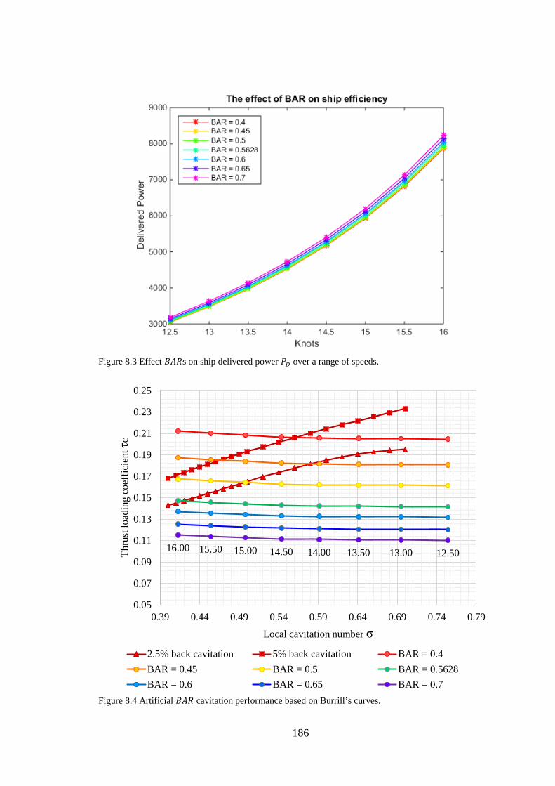
186
Figure 8.3 Effect 𝐵𝐵𝐵𝐵𝐵𝐵s on ship delivered power 𝑃𝑃𝐷𝐷 over a range of speeds.
Figure 8.4 Artificial 𝐵𝐵𝐵𝐵𝐵𝐵 cavitation performance based on Burrill’s curves.
12.5013.0013.5014.0014.5015.0015.5016.00
0.05
0.07
0.09
0.11
0.13
0.15
0.17
0.19
0.21
0.23
0.25
0.39 0.44 0.49 0.54 0.59 0.64 0.69 0.74 0.79
Thru
st lo
adin
g co
effic
ient
τc
Local cavitation number σ2.5% back cavitation 5% back cavitation BAR = 0.4BAR = 0.45 BAR = 0.5 BAR = 0.5628BAR = 0.6 BAR = 0.65 BAR = 0.7
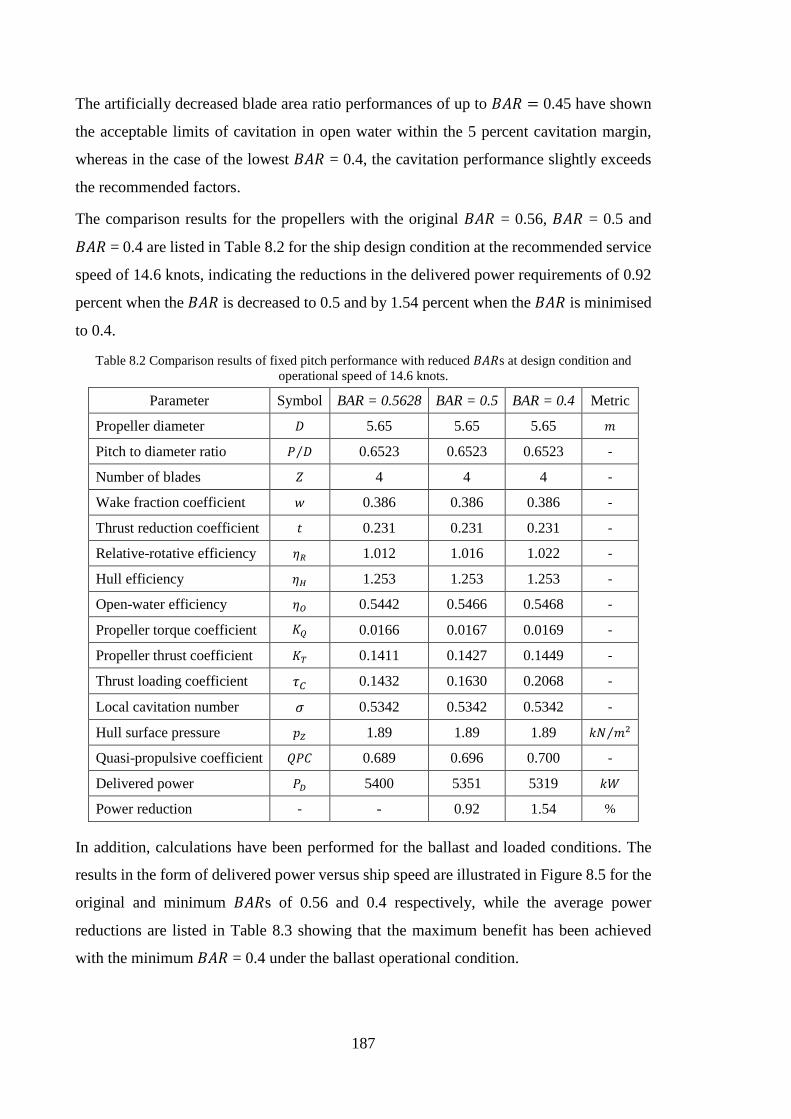
187
The artificially decreased blade area ratio performances of up to 𝐵𝐵𝐵𝐵𝐵𝐵 = 0.45 have shown
the acceptable limits of cavitation in open water within the 5 percent cavitation margin,
whereas in the case of the lowest 𝐵𝐵𝐵𝐵𝐵𝐵 = 0.4, the cavitation performance slightly exceeds
the recommended factors.
The comparison results for the propellers with the original 𝐵𝐵𝐵𝐵𝐵𝐵 = 0.56, 𝐵𝐵𝐵𝐵𝐵𝐵 = 0.5 and
𝐵𝐵𝐵𝐵𝐵𝐵 = 0.4 are listed in Table 8.2 for the ship design condition at the recommended service
speed of 14.6 knots, indicating the reductions in the delivered power requirements of 0.92
percent when the 𝐵𝐵𝐵𝐵𝐵𝐵 is decreased to 0.5 and by 1.54 percent when the 𝐵𝐵𝐵𝐵𝐵𝐵 is minimised
to 0.4.
Table 8.2 Comparison results of fixed pitch performance with reduced 𝐵𝐵𝐵𝐵𝐵𝐵s at design condition and operational speed of 14.6 knots.
Parameter Symbol BAR = 0.5628 BAR = 0.5 BAR = 0.4 Metric
Propeller diameter 𝐷𝐷 5.65 5.65 5.65 𝑛𝑛
Pitch to diameter ratio 𝑃𝑃 𝐷𝐷⁄ 0.6523 0.6523 0.6523 -
Number of blades 𝑍𝑍 4 4 4 -
Wake fraction coefficient 𝑤𝑤 0.386 0.386 0.386 -
Thrust reduction coefficient 𝐶𝐶 0.231 0.231 0.231 -
Relative-rotative efficiency 𝜂𝜂𝑅𝑅 1.012 1.016 1.022 -
Hull efficiency 𝜂𝜂𝐻𝐻 1.253 1.253 1.253 -
Open-water efficiency 𝜂𝜂𝑂𝑂 0.5442 0.5466 0.5468 -
Propeller torque coefficient 𝐾𝐾𝑄𝑄 0.0166 0.0167 0.0169 -
Propeller thrust coefficient 𝐾𝐾𝑇𝑇 0.1411 0.1427 0.1449 -
Thrust loading coefficient 𝜏𝜏𝐶𝐶 0.1432 0.1630 0.2068 -
Local cavitation number 𝜎𝜎 0.5342 0.5342 0.5342 -
Hull surface pressure 𝐶𝐶𝑍𝑍 1.89 1.89 1.89 𝑘𝑘𝑁𝑁 𝑛𝑛2⁄
Quasi-propulsive coefficient 𝑄𝑄𝑃𝑃𝐶𝐶 0.689 0.696 0.700 -
Delivered power 𝑃𝑃𝐷𝐷 5400 5351 5319 𝑘𝑘𝑊𝑊
Power reduction - - 0.92 1.54 %
In addition, calculations have been performed for the ballast and loaded conditions. The
results in the form of delivered power versus ship speed are illustrated in Figure 8.5 for the
original and minimum 𝐵𝐵𝐵𝐵𝐵𝐵s of 0.56 and 0.4 respectively, while the average power
reductions are listed in Table 8.3 showing that the maximum benefit has been achieved
with the minimum 𝐵𝐵𝐵𝐵𝐵𝐵 = 0.4 under the ballast operational condition.
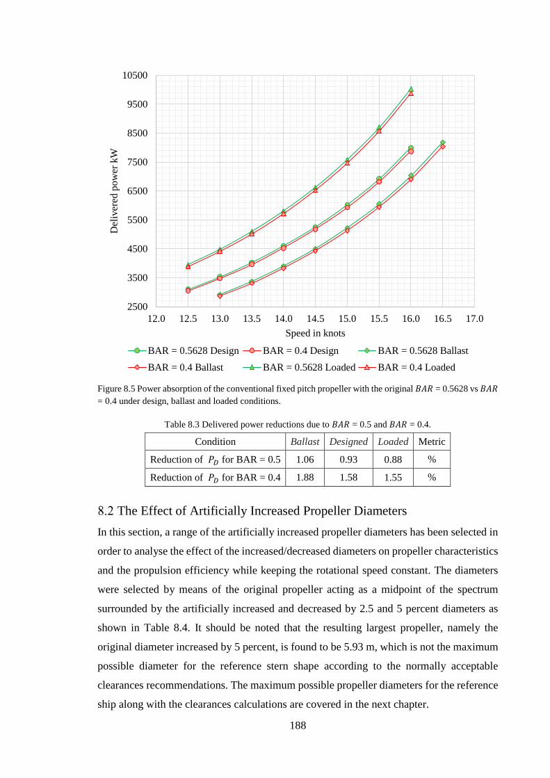
188
Figure 8.5 Power absorption of the conventional fixed pitch propeller with the original 𝐵𝐵𝐵𝐵𝐵𝐵 = 0.5628 vs 𝐵𝐵𝐵𝐵𝐵𝐵 = 0.4 under design, ballast and loaded conditions.
Table 8.3 Delivered power reductions due to 𝐵𝐵𝐵𝐵𝐵𝐵 = 0.5 and 𝐵𝐵𝐵𝐵𝐵𝐵 = 0.4.
Condition Ballast Designed Loaded Metric
Reduction of 𝑃𝑃𝐷𝐷 for BAR = 0.5 1.06 0.93 0.88 %
Reduction of 𝑃𝑃𝐷𝐷 for BAR = 0.4 1.88 1.58 1.55 %
The Effect of Artificially Increased Propeller Diameters In this section, a range of the artificially increased propeller diameters has been selected in
order to analyse the effect of the increased/decreased diameters on propeller characteristics
and the propulsion efficiency while keeping the rotational speed constant. The diameters
were selected by means of the original propeller acting as a midpoint of the spectrum
surrounded by the artificially increased and decreased by 2.5 and 5 percent diameters as
shown in Table 8.4. It should be noted that the resulting largest propeller, namely the
original diameter increased by 5 percent, is found to be 5.93 m, which is not the maximum
possible diameter for the reference stern shape according to the normally acceptable
clearances recommendations. The maximum possible propeller diameters for the reference
ship along with the clearances calculations are covered in the next chapter.
2500
3500
4500
5500
6500
7500
8500
9500
10500
12.0 12.5 13.0 13.5 14.0 14.5 15.0 15.5 16.0 16.5 17.0
Del
iver
ed p
ower
kW
Speed in knots
BAR = 0.5628 Design BAR = 0.4 Design BAR = 0.5628 BallastBAR = 0.4 Ballast BAR = 0.5628 Loaded BAR = 0.4 Loaded
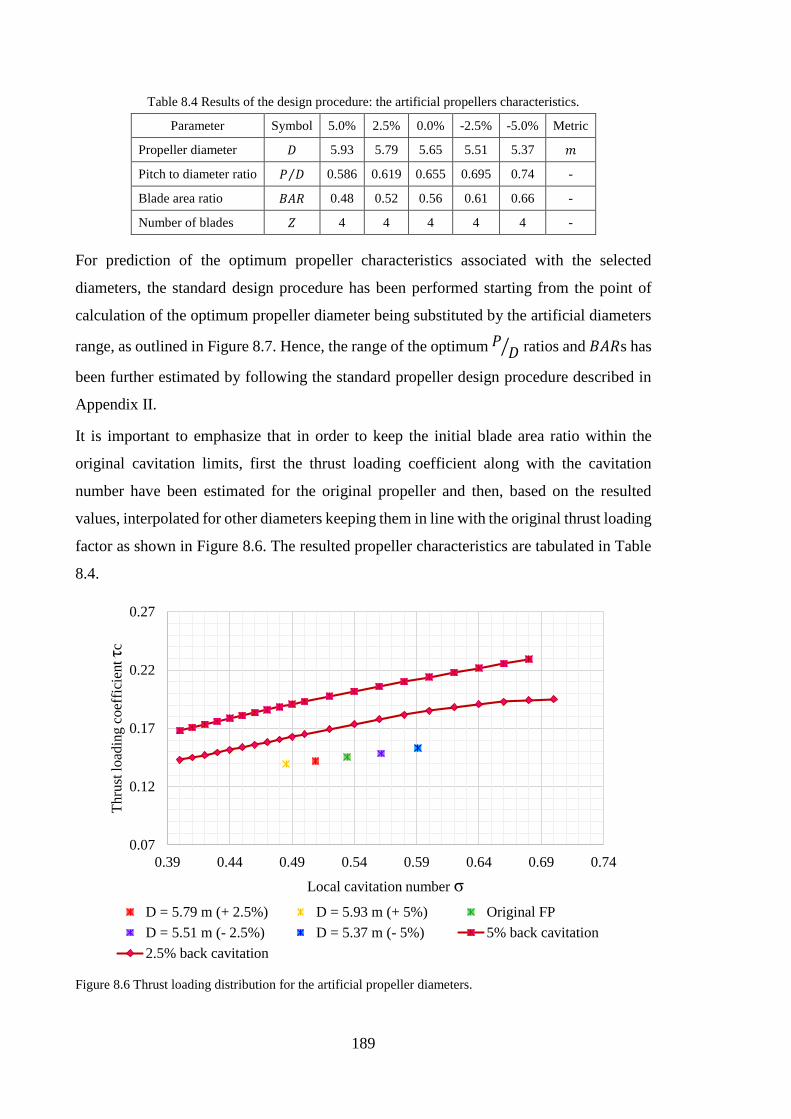
189
Table 8.4 Results of the design procedure: the artificial propellers characteristics.
Parameter Symbol 5.0% 2.5% 0.0% -2.5% -5.0% Metric
Propeller diameter 𝐷𝐷 5.93 5.79 5.65 5.51 5.37 𝑛𝑛
Pitch to diameter ratio 𝑃𝑃 𝐷𝐷⁄ 0.586 0.619 0.655 0.695 0.74 -
Blade area ratio 𝐵𝐵𝐵𝐵𝐵𝐵 0.48 0.52 0.56 0.61 0.66 -
Number of blades 𝑍𝑍 4 4 4 4 4 -
For prediction of the optimum propeller characteristics associated with the selected
diameters, the standard design procedure has been performed starting from the point of
calculation of the optimum propeller diameter being substituted by the artificial diameters
range, as outlined in Figure 8.7. Hence, the range of the optimum 𝑃𝑃 𝐷𝐷 ratios and 𝐵𝐵𝐵𝐵𝐵𝐵s has
been further estimated by following the standard propeller design procedure described in
Appendix II.
It is important to emphasize that in order to keep the initial blade area ratio within the
original cavitation limits, first the thrust loading coefficient along with the cavitation
number have been estimated for the original propeller and then, based on the resulted
values, interpolated for other diameters keeping them in line with the original thrust loading
factor as shown in Figure 8.6. The resulted propeller characteristics are tabulated in Table
8.4.
Figure 8.6 Thrust loading distribution for the artificial propeller diameters.
0.07
0.12
0.17
0.22
0.27
0.39 0.44 0.49 0.54 0.59 0.64 0.69 0.74
Thru
st lo
adin
g co
effic
ient
τc
Local cavitation number σD = 5.79 m (+ 2.5%) D = 5.93 m (+ 5%) Original FPD = 5.51 m (- 2.5%) D = 5.37 m (- 5%) 5% back cavitation2.5% back cavitation
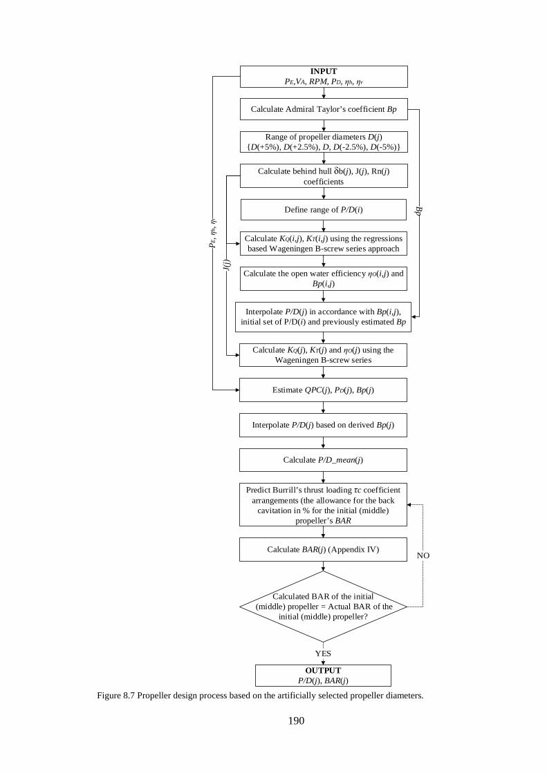
190
INPUTPE,VA, RPM, PD, ηh, ηr
Calculate behind hull δb(j), J(j), Rn(j) coefficients
Range of propeller diameters D(j)D(+5%), D(+2.5%), D, D(-2.5%), D(-5%)
Define range of P/D(i)
Calculate KQ(i,j), KT(i,j) using the regressions based Wageningen B-screw series approach
Interpolate P/D(j) in accordance with Bp(i,j), initial set of P/D(i) and previously estimated Bp
Calculate KQ(j), KT(j) and ηO(j) using the Wageningen B-screw series
Estimate QPC(j), PD(j), Bp(j)
Interpolate P/D(j) based on derived Bp(j)
Calculate P/D_mean(j)
Predict Burrill’s thrust loading τc coefficient arrangements (the allowance for the back
cavitation in % for the initial (middle) propeller’s BAR
OUTPUT P/D(j), BAR(j)
Calculate Admiral Taylor’s coefficient Bp
Calculate the open water efficiency ηO(i,j) and Bp(i,j)
Bp
J(j)
PE, η
h, ηr
Calculated BAR of the initial (middle) propeller = Actual BAR of the
initial (middle) propeller?
Calculate BAR(j) (Appendix IV)
YES
NO
Figure 8.7 Propeller design process based on the artificially selected propeller diameters.
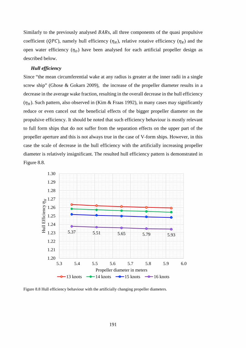
191
Similarly to the previously analysed 𝐵𝐵𝐵𝐵𝐵𝐵s, all three components of the quasi propulsive
coefficient (𝑄𝑄𝑃𝑃𝐶𝐶), namely hull efficiency (𝜂𝜂𝐻𝐻), relative rotative efficiency (𝜂𝜂𝑅𝑅) and the
open water efficiency (𝜂𝜂𝑂𝑂) have been analysed for each artificial propeller design as
described below.
Hull efficiency
Since “the mean circumferential wake at any radius is greater at the inner radii in a single
screw ship” (Ghose & Gokarn 2009), the increase of the propeller diameter results in a
decrease in the average wake fraction, resulting in the overall decrease in the hull efficiency
(𝜂𝜂𝐻𝐻). Such pattern, also observed in (Kim & Fraas 1992), in many cases may significantly
reduce or even cancel out the beneficial effects of the bigger propeller diameter on the
propulsive efficiency. It should be noted that such efficiency behaviour is mostly relevant
to full form ships that do not suffer from the separation effects on the upper part of the
propeller aperture and this is not always true in the case of V-form ships. However, in this
case the scale of decrease in the hull efficiency with the artificially increasing propeller
diameter is relatively insignificant. The resulted hull efficiency pattern is demonstrated in
Figure 8.8.
Figure 8.8 Hull efficiency behaviour with the artificially changing propeller diameters.
5.935.795.655.515.37
1.20
1.21
1.22
1.23
1.24
1.25
1.26
1.27
1.28
1.29
1.30
5.3 5.4 5.5 5.6 5.7 5.8 5.9 6.0
Hul
l Eff
icie
ncy 𝜂𝜂 𝐻𝐻
Propeller diameter in meters13 knots 14 knots 15 knots 16 knots
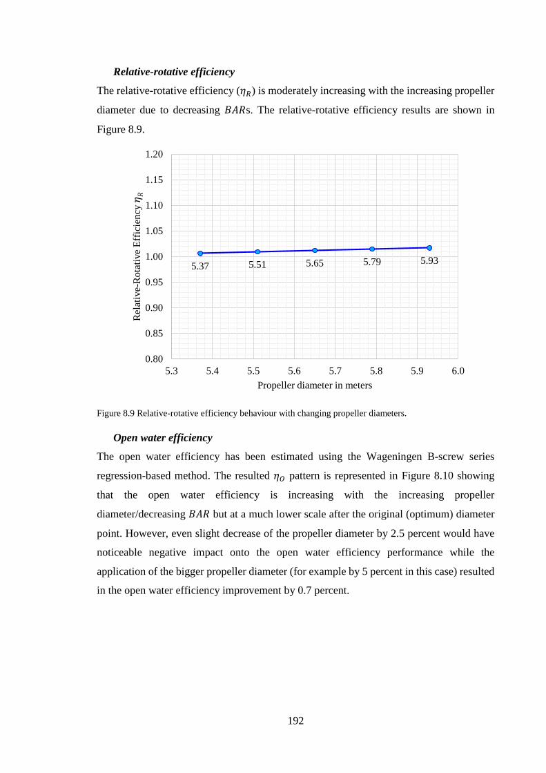
192
Relative-rotative efficiency
The relative-rotative efficiency (𝜂𝜂𝑅𝑅) is moderately increasing with the increasing propeller
diameter due to decreasing 𝐵𝐵𝐵𝐵𝐵𝐵s. The relative-rotative efficiency results are shown in
Figure 8.9.
Figure 8.9 Relative-rotative efficiency behaviour with changing propeller diameters.
Open water efficiency
The open water efficiency has been estimated using the Wageningen B-screw series
regression-based method. The resulted 𝜂𝜂𝑂𝑂 pattern is represented in Figure 8.10 showing
that the open water efficiency is increasing with the increasing propeller
diameter/decreasing 𝐵𝐵𝐵𝐵𝐵𝐵 but at a much lower scale after the original (optimum) diameter
point. However, even slight decrease of the propeller diameter by 2.5 percent would have
noticeable negative impact onto the open water efficiency performance while the
application of the bigger propeller diameter (for example by 5 percent in this case) resulted
in the open water efficiency improvement by 0.7 percent.
5.935.795.655.515.37
0.80
0.85
0.90
0.95
1.00
1.05
1.10
1.15
1.20
5.3 5.4 5.5 5.6 5.7 5.8 5.9 6.0
Rel
ativ
e-R
otat
ive
Effic
ienc
y 𝜂𝜂 𝐵𝐵
Propeller diameter in meters
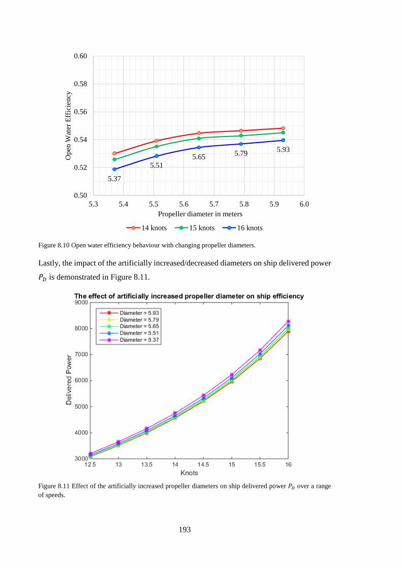
193
Figure 8.10 Open water efficiency behaviour with changing propeller diameters.
Lastly, the impact of the artificially increased/decreased diameters on ship delivered power
𝑃𝑃𝐷𝐷 is demonstrated in Figure 8.11.
Figure 8.11 Effect of the artificially increased propeller diameters on ship delivered power 𝑃𝑃𝐷𝐷 over a range of speeds.
5.935.795.655.51
5.37
0.50
0.52
0.54
0.56
0.58
0.60
5.3 5.4 5.5 5.6 5.7 5.8 5.9 6.0
Ope
n W
ater
Eff
icie
ncy
Propeller diameter in meters
14 knots 15 knots 16 knots
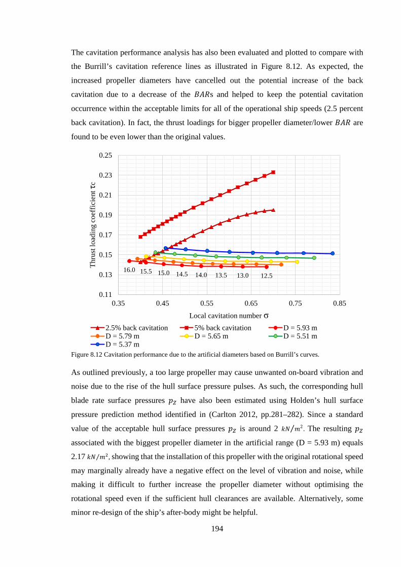
194
The cavitation performance analysis has also been evaluated and plotted to compare with
the Burrill’s cavitation reference lines as illustrated in Figure 8.12. As expected, the
increased propeller diameters have cancelled out the potential increase of the back
cavitation due to a decrease of the 𝐵𝐵𝐵𝐵𝐵𝐵s and helped to keep the potential cavitation
occurrence within the acceptable limits for all of the operational ship speeds (2.5 percent
back cavitation). In fact, the thrust loadings for bigger propeller diameter/lower 𝐵𝐵𝐵𝐵𝐵𝐵 are
found to be even lower than the original values.
Figure 8.12 Cavitation performance due to the artificial diameters based on Burrill’s curves.
As outlined previously, a too large propeller may cause unwanted on-board vibration and
noise due to the rise of the hull surface pressure pulses. As such, the corresponding hull
blade rate surface pressures 𝐶𝐶𝑍𝑍 have also been estimated using Holden’s hull surface
pressure prediction method identified in (Carlton 2012, pp.281–282). Since a standard
value of the acceptable hull surface pressures 𝐶𝐶𝑍𝑍 is around 2 𝑘𝑘𝑁𝑁 𝑛𝑛2⁄ . The resulting 𝐶𝐶𝑍𝑍
associated with the biggest propeller diameter in the artificial range (D = 5.93 m) equals
2.17 𝑘𝑘𝑁𝑁 𝑛𝑛2⁄ , showing that the installation of this propeller with the original rotational speed
may marginally already have a negative effect on the level of vibration and noise, while
making it difficult to further increase the propeller diameter without optimising the
rotational speed even if the sufficient hull clearances are available. Alternatively, some
minor re-design of the ship’s after-body might be helpful.
12.513.013.514.014.515.015.516.0
0.11
0.13
0.15
0.17
0.19
0.21
0.23
0.25
0.35 0.45 0.55 0.65 0.75 0.85
Thru
st lo
adin
g co
effic
ient
τc
Local cavitation number σ2.5% back cavitation 5% back cavitation D = 5.93 mD = 5.79 m D = 5.65 m D = 5.51 mD = 5.37 m
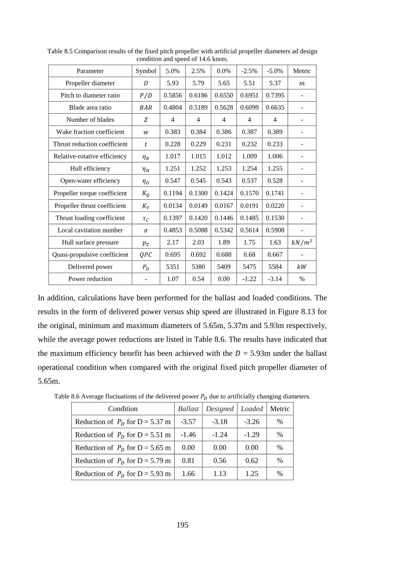
195
Table 8.5 Comparison results of the fixed pitch propeller with artificial propeller diameters ad design condition and speed of 14.6 knots.
Parameter Symbol 5.0% 2.5% 0.0% -2.5% -5.0% Metric
Propeller diameter 𝐷𝐷 5.93 5.79 5.65 5.51 5.37 𝑛𝑛
Pitch to diameter ratio 𝑃𝑃 𝐷𝐷⁄ 0.5856 0.6186 0.6550 0.6951 0.7395 -
Blade area ratio 𝐵𝐵𝐵𝐵𝐵𝐵 0.4804 0.5189 0.5628 0.6099 0.6635 -
Number of blades 𝑍𝑍 4 4 4 4 4 -
Wake fraction coefficient 𝑤𝑤 0.383 0.384 0.386 0.387 0.389 -
Thrust reduction coefficient 𝐶𝐶 0.228 0.229 0.231 0.232 0.233 -
Relative-rotative efficiency 𝜂𝜂𝑅𝑅 1.017 1.015 1.012 1.009 1.006 -
Hull efficiency 𝜂𝜂𝐻𝐻 1.251 1.252 1.253 1.254 1.255 -
Open-water efficiency 𝜂𝜂𝑂𝑂 0.547 0.545 0.543 0.537 0.528 -
Propeller torque coefficient 𝐾𝐾𝑄𝑄 0.1194 0.1300 0.1424 0.1570 0.1741 -
Propeller thrust coefficient 𝐾𝐾𝑇𝑇 0.0134 0.0149 0.0167 0.0191 0.0220 -
Thrust loading coefficient 𝜏𝜏𝐶𝐶 0.1397 0.1420 0.1446 0.1485 0.1530 -
Local cavitation number 𝜎𝜎 0.4853 0.5088 0.5342 0.5614 0.5908 -
Hull surface pressure 𝐶𝐶𝑍𝑍 2.17 2.03 1.89 1.75 1.63 𝑘𝑘𝑁𝑁 𝑛𝑛2⁄
Quasi-propulsive coefficient 𝑄𝑄𝑃𝑃𝐶𝐶 0.695 0.692 0.688 0.68 0.667 -
Delivered power 𝑃𝑃𝐷𝐷 5351 5380 5409 5475 5584 𝑘𝑘𝑊𝑊
Power reduction - 1.07 0.54 0.00 -1.22 -3.14 %
In addition, calculations have been performed for the ballast and loaded conditions. The
results in the form of delivered power versus ship speed are illustrated in Figure 8.13 for
the original, minimum and maximum diameters of 5.65m, 5.37m and 5.93m respectively,
while the average power reductions are listed in Table 8.6. The results have indicated that
the maximum efficiency benefit has been achieved with the 𝐷𝐷 = 5.93m under the ballast
operational condition when compared with the original fixed pitch propeller diameter of
5.65m.
Table 8.6 Average fluctuations of the delivered power 𝑃𝑃𝐷𝐷 due to artificially changing diameters.
Condition Ballast Designed Loaded Metric
Reduction of 𝑃𝑃𝐷𝐷 for D = 5.37 m -3.57 -3.18 -3.26 %
Reduction of 𝑃𝑃𝐷𝐷 for D = 5.51 m -1.46 -1.24 -1.29 %
Reduction of 𝑃𝑃𝐷𝐷 for D = 5.65 m 0.00 0.00 0.00 %
Reduction of 𝑃𝑃𝐷𝐷 for D = 5.79 m 0.81 0.56 0.62 %
Reduction of 𝑃𝑃𝐷𝐷 for D = 5.93 m 1.66 1.13 1.25 %
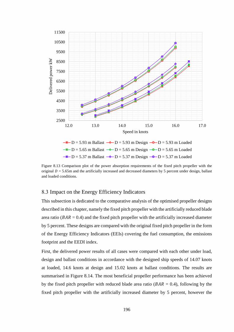
196
Figure 8.13 Comparison plot of the power absorption requirements of the fixed pitch propeller with the original 𝐷𝐷 = 5.65m and the artificially increased and decreased diameters by 5 percent under design, ballast and loaded conditions.
Impact on the Energy Efficiency Indicators This subsection is dedicated to the comparative analysis of the optimised propeller designs
described in this chapter, namely the fixed pitch propeller with the artificially reduced blade
area ratio (𝐵𝐵𝐵𝐵𝐵𝐵 = 0.4) and the fixed pitch propeller with the artificially increased diameter
by 5 percent. These designs are compared with the original fixed pitch propeller in the form
of the Energy Efficiency Indicators (EEIs) covering the fuel consumption, the emissions
footprint and the EEDI index.
First, the delivered power results of all cases were compared with each other under load,
design and ballast conditions in accordance with the designed ship speeds of 14.07 knots
at loaded, 14.6 knots at design and 15.02 knots at ballast conditions. The results are
summarised in Figure 8.14. The most beneficial propeller performance has been achieved
by the fixed pitch propeller with reduced blade area ratio (𝐵𝐵𝐵𝐵𝐵𝐵 = 0.4), following by the
fixed pitch propeller with the artificially increased diameter by 5 percent, however the
2500
3500
4500
5500
6500
7500
8500
9500
10500
11500
12.0 13.0 14.0 15.0 16.0 17.0
Del
iver
ed p
ower
kW
Speed in knots
D = 5.93 m Ballast D = 5.93 m Design D = 5.93 m LoadedD = 5.65 m Ballast D = 5.65 m Design D = 5.65 m LoadedD = 5.37 m Ballast D = 5.37 m Design D = 5.37 m Loaded
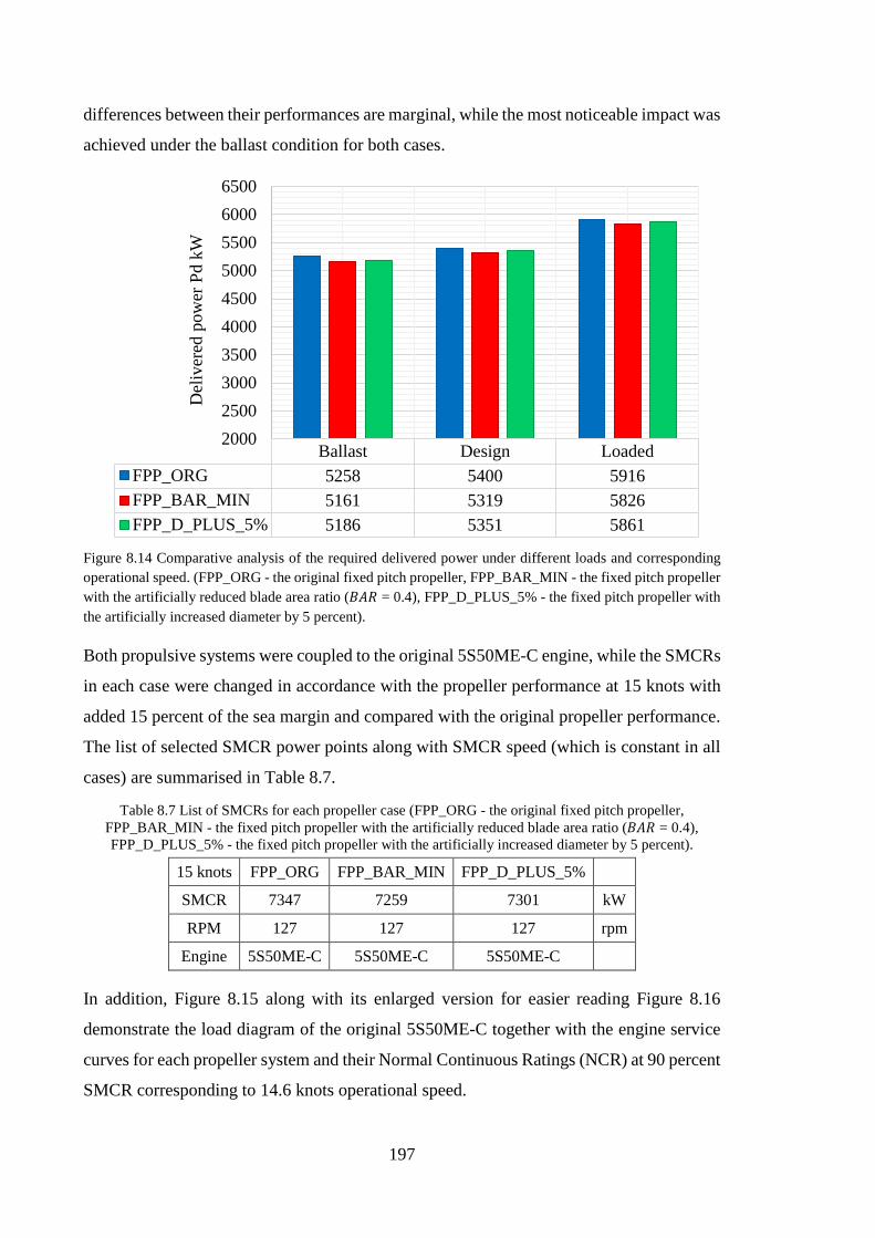
197
differences between their performances are marginal, while the most noticeable impact was
achieved under the ballast condition for both cases.
Figure 8.14 Comparative analysis of the required delivered power under different loads and corresponding operational speed. (FPP_ORG - the original fixed pitch propeller, FPP_BAR_MIN - the fixed pitch propeller with the artificially reduced blade area ratio (𝐵𝐵𝐵𝐵𝐵𝐵 = 0.4), FPP_D_PLUS_5% - the fixed pitch propeller with the artificially increased diameter by 5 percent).
Both propulsive systems were coupled to the original 5S50ME-C engine, while the SMCRs
in each case were changed in accordance with the propeller performance at 15 knots with
added 15 percent of the sea margin and compared with the original propeller performance.
The list of selected SMCR power points along with SMCR speed (which is constant in all
cases) are summarised in Table 8.7.
Table 8.7 List of SMCRs for each propeller case (FPP_ORG - the original fixed pitch propeller, FPP_BAR_MIN - the fixed pitch propeller with the artificially reduced blade area ratio (𝐵𝐵𝐵𝐵𝐵𝐵 = 0.4), FPP_D_PLUS_5% - the fixed pitch propeller with the artificially increased diameter by 5 percent).
15 knots FPP_ORG FPP_BAR_MIN FPP_D_PLUS_5%
SMCR 7347 7259 7301 kW
RPM 127 127 127 rpm
Engine 5S50ME-C 5S50ME-C 5S50ME-C
In addition, Figure 8.15 along with its enlarged version for easier reading Figure 8.16
demonstrate the load diagram of the original 5S50ME-C together with the engine service
curves for each propeller system and their Normal Continuous Ratings (NCR) at 90 percent
SMCR corresponding to 14.6 knots operational speed.
Ballast Design LoadedFPP_ORG 5258 5400 5916FPP_BAR_MIN 5161 5319 5826FPP_D_PLUS_5% 5186 5351 5861
2000250030003500400045005000550060006500
Del
iver
ed p
ower
Pd
kW
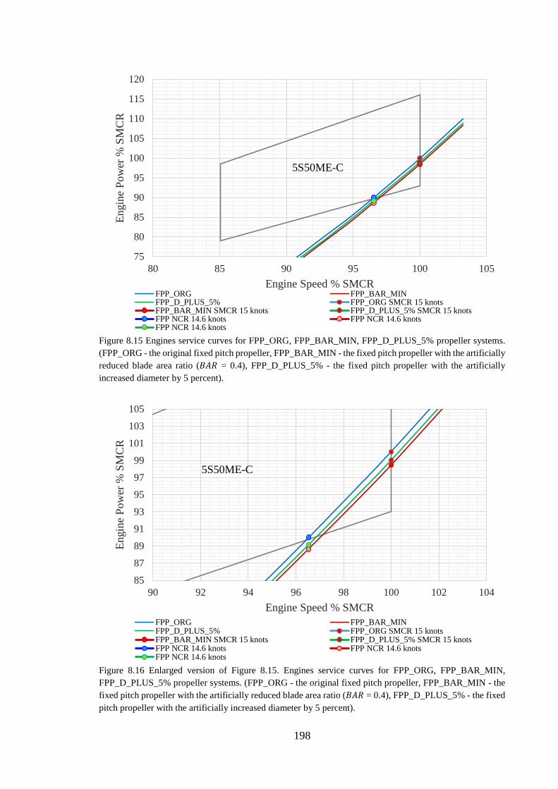
198
Figure 8.15 Engines service curves for FPP_ORG, FPP_BAR_MIN, FPP_D_PLUS_5% propeller systems. (FPP_ORG - the original fixed pitch propeller, FPP_BAR_MIN - the fixed pitch propeller with the artificially reduced blade area ratio (𝐵𝐵𝐵𝐵𝐵𝐵 = 0.4), FPP_D_PLUS_5% - the fixed pitch propeller with the artificially increased diameter by 5 percent).
Figure 8.16 Enlarged version of Figure 8.15. Engines service curves for FPP_ORG, FPP_BAR_MIN, FPP_D_PLUS_5% propeller systems. (FPP_ORG - the original fixed pitch propeller, FPP_BAR_MIN - the fixed pitch propeller with the artificially reduced blade area ratio (𝐵𝐵𝐵𝐵𝐵𝐵 = 0.4), FPP_D_PLUS_5% - the fixed pitch propeller with the artificially increased diameter by 5 percent).
75
80
85
90
95
100
105
110
115
120
80 85 90 95 100 105
Engi
ne P
ower
% S
MC
R
Engine Speed % SMCRFPP_ORG FPP_BAR_MINFPP_D_PLUS_5% FPP_ORG SMCR 15 knotsFPP_BAR_MIN SMCR 15 knots FPP_D_PLUS_5% SMCR 15 knotsFPP NCR 14.6 knots FPP NCR 14.6 knotsFPP NCR 14.6 knots
5S50ME-C
8587899193959799
101103105
90 92 94 96 98 100 102 104
Engi
ne P
ower
% S
MC
R
Engine Speed % SMCRFPP_ORG FPP_BAR_MINFPP_D_PLUS_5% FPP_ORG SMCR 15 knotsFPP_BAR_MIN SMCR 15 knots FPP_D_PLUS_5% SMCR 15 knotsFPP NCR 14.6 knots FPP NCR 14.6 knotsFPP NCR 14.6 knots
5S50ME-C
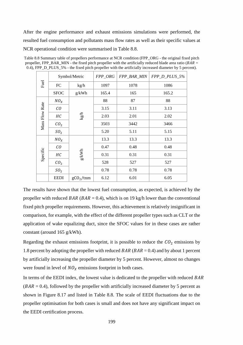
199
After the engine performance and exhaust emissions simulations were performed, the
resulted fuel consumption and pollutants mass flow rates as well as their specific values at
NCR operational condition were summarised in Table 8.8.
Table 8.8 Summary table of propellers performance at NCR condition (FPP_ORG - the original fixed pitch propeller, FPP_BAR_MIN - the fixed pitch propeller with the artificially reduced blade area ratio (𝐵𝐵𝐵𝐵𝐵𝐵 = 0.4), FPP_D_PLUS_5% - the fixed pitch propeller with the artificially increased diameter by 5 percent).
Fuel
Symbol/Metric FPP_ORG FPP_BAR_MIN FPP_D_PLUS_5%
FC kg/h 1097 1078 1086
SFOC g/kWh 165.4 165 165.2
Mas
s Flo
w R
ate 𝑁𝑁𝐶𝐶𝑋𝑋
kg/h
88 87 88
𝐶𝐶𝐶𝐶 3.15 3.11 3.13
𝐻𝐻𝐶𝐶 2.03 2.01 2.02
𝐶𝐶𝐶𝐶2 3503 3442 3466
𝑆𝑆𝐶𝐶2 5.20 5.11 5.15
Spec
ific
𝑁𝑁𝐶𝐶𝑋𝑋
g/kW
h
13.3 13.3 13.3
𝐶𝐶𝐶𝐶 0.47 0.48 0.48
𝐻𝐻𝐶𝐶 0.31 0.31 0.31
𝐶𝐶𝐶𝐶2 528 527 527
𝑆𝑆𝐶𝐶2 0.78 0.78 0.78
EEDI gCO2/tnm 6.12 6.01 6.05
The results have shown that the lowest fuel consumption, as expected, is achieved by the
propeller with reduced 𝐵𝐵𝐵𝐵𝐵𝐵 (𝐵𝐵𝐵𝐵𝐵𝐵 = 0.4), which is on 19 kg/h lower than the conventional
fixed pitch propeller requirements. However, this achievement is relatively insignificant in
comparison, for example, with the effect of the different propeller types such as CLT or the
application of wake equalizing duct, since the SFOC values for in these cases are rather
constant (around 165 g/kWh).
Regarding the exhaust emissions footprint, it is possible to reduce the 𝐶𝐶𝐶𝐶2 emissions by
1.8 percent by adopting the propeller with reduced 𝐵𝐵𝐵𝐵𝐵𝐵 (𝐵𝐵𝐵𝐵𝐵𝐵 = 0.4) and by about 1 percent
by artificially increasing the propeller diameter by 5 percent. However, almost no changes
were found in level of 𝑁𝑁𝐶𝐶𝑋𝑋 emissions footprint in both cases.
In terms of the EEDI index, the lowest value is dedicated to the propeller with reduced 𝐵𝐵𝐵𝐵𝐵𝐵
(𝐵𝐵𝐵𝐵𝐵𝐵 = 0.4), followed by the propeller with artificially increased diameter by 5 percent as
shown in Figure 8.17 and listed in Table 8.8. The scale of EEDI fluctuations due to the
propeller optimisation for both cases is small and does not have any significant impact on
the EEDI certification process.
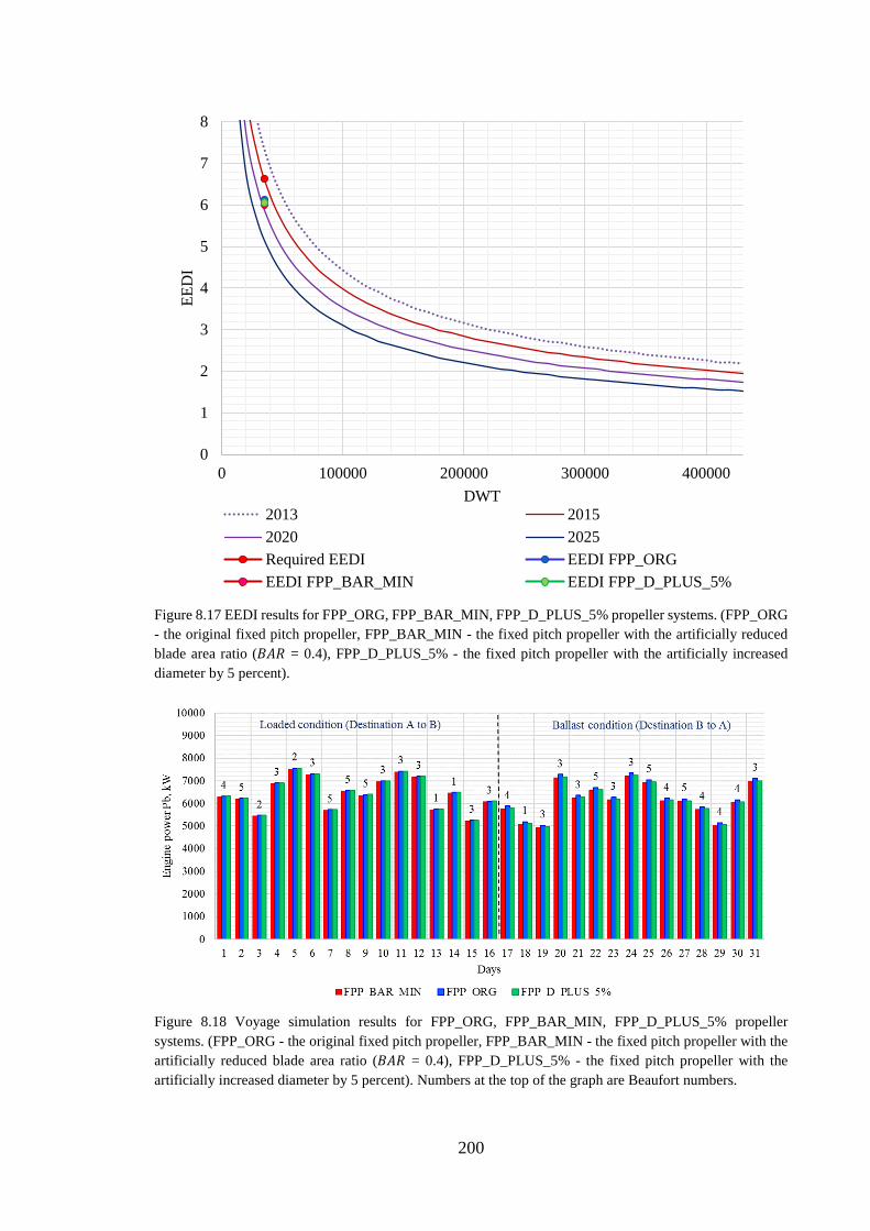
200
Figure 8.17 EEDI results for FPP_ORG, FPP_BAR_MIN, FPP_D_PLUS_5% propeller systems. (FPP_ORG - the original fixed pitch propeller, FPP_BAR_MIN - the fixed pitch propeller with the artificially reduced blade area ratio (𝐵𝐵𝐵𝐵𝐵𝐵 = 0.4), FPP_D_PLUS_5% - the fixed pitch propeller with the artificially increased diameter by 5 percent).
Figure 8.18 Voyage simulation results for FPP_ORG, FPP_BAR_MIN, FPP_D_PLUS_5% propeller systems. (FPP_ORG - the original fixed pitch propeller, FPP_BAR_MIN - the fixed pitch propeller with the artificially reduced blade area ratio (𝐵𝐵𝐵𝐵𝐵𝐵 = 0.4), FPP_D_PLUS_5% - the fixed pitch propeller with the artificially increased diameter by 5 percent). Numbers at the top of the graph are Beaufort numbers.
0
1
2
3
4
5
6
7
8
0 100000 200000 300000 400000
EED
I
DWT2013 20152020 2025Required EEDI EEDI FPP_ORGEEDI FPP_BAR_MIN EEDI FPP_D_PLUS_5%
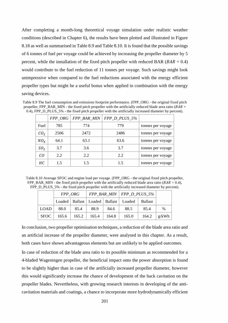
201
After completing a month-long theoretical voyage simulation under realistic weather
conditions (described in Chapter 6), the results have been plotted and illustrated in Figure
8.18 as well as summarised in Table 8.9 and Table 8.10. It is found that the possible savings
of 6 tonnes of fuel per voyage could be achieved by increasing the propeller diameter by 5
percent, while the installation of the fixed pitch propeller with reduced BAR (𝐵𝐵𝐵𝐵𝐵𝐵 = 0.4)
would contribute to the fuel reduction of 11 tonnes per voyage. Such savings might look
unimpressive when compared to the fuel reductions associated with the energy efficient
propeller types but might be a useful bonus when applied in combination with the energy
saving devices.
Table 8.9 The fuel consumption and emissions footprint performance. (FPP_ORG - the original fixed pitch propeller, FPP_BAR_MIN - the fixed pitch propeller with the artificially reduced blade area ratio (𝐵𝐵𝐵𝐵𝐵𝐵 =
0.4), FPP_D_PLUS_5% - the fixed pitch propeller with the artificially increased diameter by percent).
FPP_ORG FPP_BAR_MIN FPP_D_PLUS_5%
Fuel 785 774 779 tonnes per voyage
𝐶𝐶𝐶𝐶2 2506 2472 2486 tonnes per voyage
𝑁𝑁𝐶𝐶𝑋𝑋 64.1 63.1 63.6 tonnes per voyage
𝑆𝑆𝐶𝐶2 3.7 3.6 3.7 tonnes per voyage
𝐶𝐶𝐶𝐶 2.2 2.2 2.2 tonnes per voyage
𝐻𝐻𝐶𝐶 1.5 1.5 1.5 tonnes per voyage
Table 8.10 Average SFOC and engine load per voyage. (FPP_ORG - the original fixed pitch propeller, FPP_BAR_MIN - the fixed pitch propeller with the artificially reduced blade area ratio (𝐵𝐵𝐵𝐵𝐵𝐵 = 0.4),
FPP_D_PLUS_5% - the fixed pitch propeller with the artificially increased diameter by percent).
FPP_ORG FPP_BAR_MIN FPP_D_PLUS_5%
Loaded Ballast Loaded Ballast Loaded Ballast
LOAD 88.0 85.4 88.9 84.6 88.5 85.4 %
SFOC 165.6 165.2 165.4 164.8 165.0 164.2 g/kWh
In conclusion, two propeller optimisation techniques, a reduction of the blade area ratio and
an artificial increase of the propeller diameter, were analysed in this chapter. As a result,
both cases have shown advantageous elements but are unlikely to be applied outcomes.
In case of reduction of the blade area ratio to its possible minimum as recommended for a
4-bladed Wageningen propeller, the beneficial impact onto the power absorption is found
to be slightly higher than in case of the artificially increased propeller diameter, however
this would significantly increase the chance of development of the back cavitation on the
propeller blades. Nevertheless, with growing research interests in developing of the anti-
cavitation materials and coatings, a chance to incorporate more hydrodynamically efficient

202
propellers with reduced blade area ratio without the fear of cavitation will significantly
increase. The foregoing results suggest that further work is necessary for understanding the
margins against cavitation erosion.
In turn, the artificially increased propeller diameter has also shown a positive influence on
the overall propulsive efficiency, although slightly lower than in the case of the reduction
of blade area ratio. Nevertheless, the increase of the propeller diameter (with decreasing
𝐵𝐵𝐵𝐵𝐵𝐵) will not affect the cavitation performance since the excessive thrust loading would
be evenly distributed along a larger surface of the propeller disk. However, even 5 percent
increase of the optimum diameter will give a minor rise to the hull surface pressure pulses,
resulting in potential intensification of the inboard noise and vibration.
The analysis of the energy efficiency indicators (EEIs) has shown that the application of
such propeller systems alone will not significantly affect the emissions footprint and the
EEDI index, however, will provide some fuel savings which might be a useful bonus when
combined with other energy saving devices.
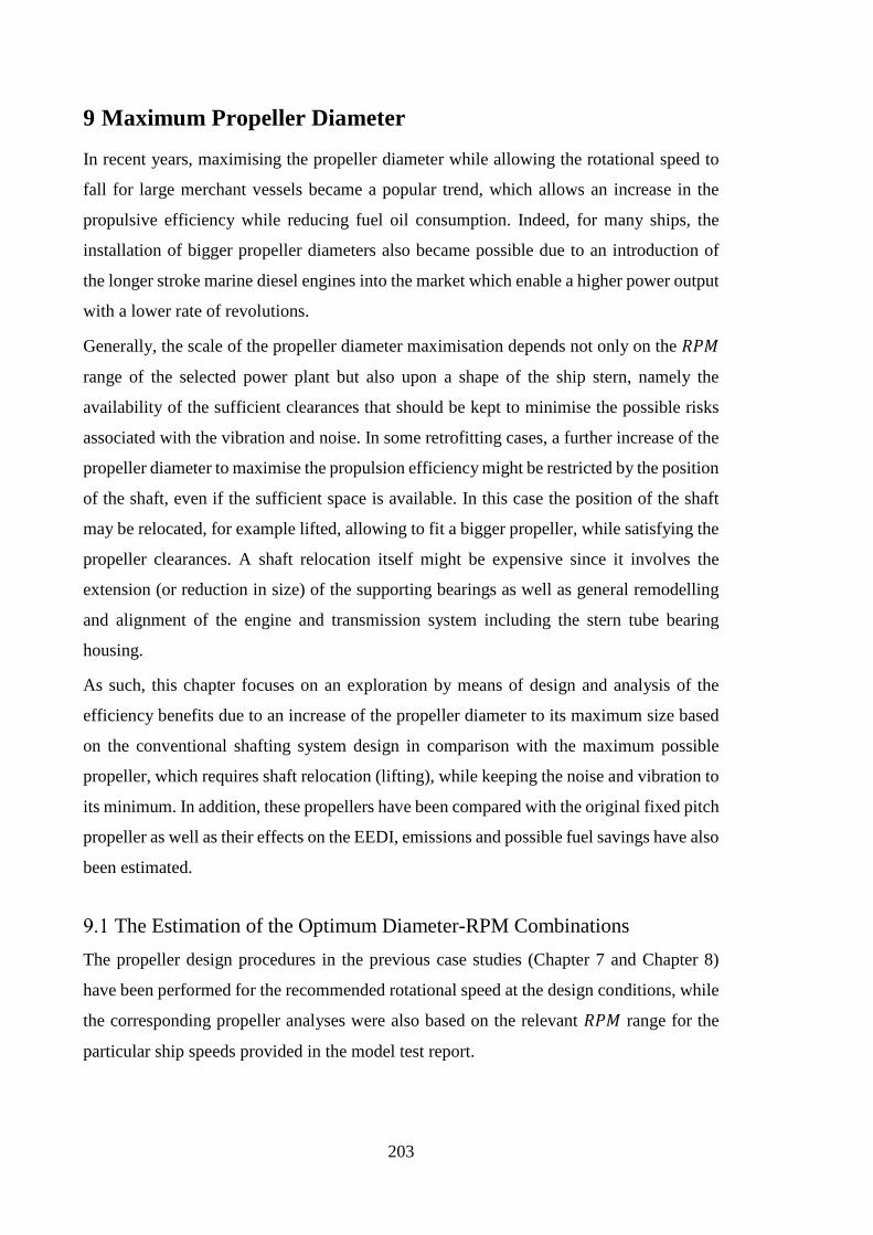
203
9 Maximum Propeller Diameter
In recent years, maximising the propeller diameter while allowing the rotational speed to
fall for large merchant vessels became a popular trend, which allows an increase in the
propulsive efficiency while reducing fuel oil consumption. Indeed, for many ships, the
installation of bigger propeller diameters also became possible due to an introduction of
the longer stroke marine diesel engines into the market which enable a higher power output
with a lower rate of revolutions.
Generally, the scale of the propeller diameter maximisation depends not only on the 𝐵𝐵𝑃𝑃𝑁𝑁
range of the selected power plant but also upon a shape of the ship stern, namely the
availability of the sufficient clearances that should be kept to minimise the possible risks
associated with the vibration and noise. In some retrofitting cases, a further increase of the
propeller diameter to maximise the propulsion efficiency might be restricted by the position
of the shaft, even if the sufficient space is available. In this case the position of the shaft
may be relocated, for example lifted, allowing to fit a bigger propeller, while satisfying the
propeller clearances. A shaft relocation itself might be expensive since it involves the
extension (or reduction in size) of the supporting bearings as well as general remodelling
and alignment of the engine and transmission system including the stern tube bearing
housing.
As such, this chapter focuses on an exploration by means of design and analysis of the
efficiency benefits due to an increase of the propeller diameter to its maximum size based
on the conventional shafting system design in comparison with the maximum possible
propeller, which requires shaft relocation (lifting), while keeping the noise and vibration to
its minimum. In addition, these propellers have been compared with the original fixed pitch
propeller as well as their effects on the EEDI, emissions and possible fuel savings have also
been estimated.
The Estimation of the Optimum Diameter-RPM Combinations The propeller design procedures in the previous case studies (Chapter 7 and Chapter 8)
have been performed for the recommended rotational speed at the design conditions, while
the corresponding propeller analyses were also based on the relevant 𝐵𝐵𝑃𝑃𝑁𝑁 range for the
particular ship speeds provided in the model test report.
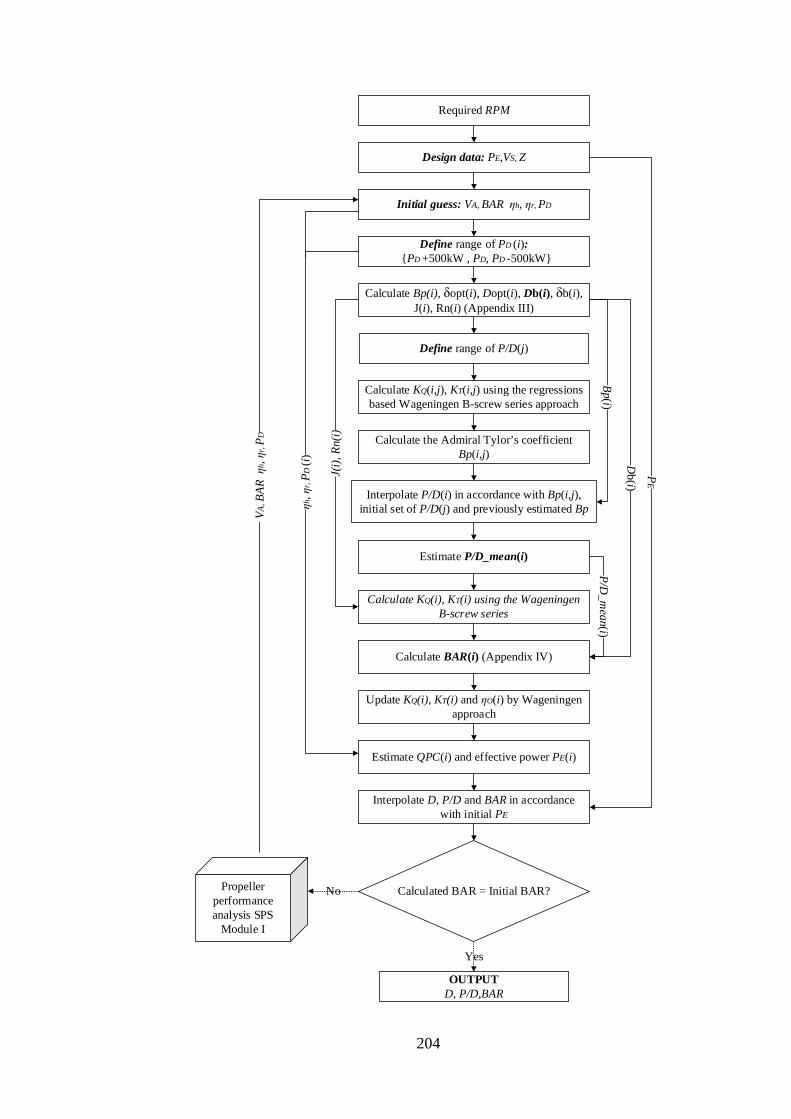
204
Design data: PE,VS, Z
Calculate KQ(i), KT(i) using the Wageningen B-screw series
OUTPUT D, P/D,BAR
Calculate the Admiral Tylor’s coefficient Bp(i,j)
Bp(i)
J(i),
Rn(
i)
Required RPM
Initial guess: VA, BAR ηh, ηr, PD
Define range of PD (i): PD +500kW , PD, PD -500kW
Calculate Bp(i), δopt(i), Dopt(i), Db(i), δb(i), J(i), Rn(i) (Appendix III)
Define range of P/D(j)
Calculate KQ(i,j), KT(i,j) using the regressions based Wageningen B-screw series approach
Interpolate P/D(i) in accordance with Bp(i,j), initial set of P/D(j) and previously estimated Bp
Calculate BAR(i) (Appendix IV)
Update KQ(i), KT(i) and ηO(i) by Wageningen approach
Db(i)
Estimate P/D_mean(i)
P/D_m
ean(i)
Estimate QPC(i) and effective power PE(i)
ηh, η
r, PD
(i)
Interpolate D, P/D and BAR in accordance with initial PE
PE
Calculated BAR = Initial BAR? Propeller performance analysis SPS
Module I
VA,
BAR
ηh,
ηr, P
D
No
Yes
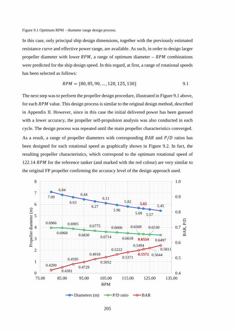
205
Figure 9.1 Optimum RPM – diameter range design process.
In this case, only principal ship design dimensions, together with the previously estimated
resistance curve and effective power range, are available. As such, in order to design larger
propeller diameter with lower 𝐵𝐵𝑃𝑃𝑁𝑁, a range of optimum diameter – 𝐵𝐵𝑃𝑃𝑁𝑁 combinations
were predicted for the ship design speed. In this regard, at first, a range of rotational speeds
has been selected as follows:
𝐵𝐵𝑃𝑃𝑁𝑁 = 80, 85, 90, … , 120, 125, 130 9.1
The next step was to perform the propeller design procedure, illustrated in Figure 9.1 above,
for each 𝐵𝐵𝑃𝑃𝑁𝑁 value. This design process is similar to the original design method, described
in Appendix II. However, since in this case the initial delivered power has been guessed
with a lower accuracy, the propeller self-propulsion analysis was also conducted in each
cycle. The design process was repeated until the main propeller characteristics converged.
As a result, a range of propeller diameters with corresponding 𝐵𝐵𝐵𝐵𝐵𝐵 and 𝑃𝑃/𝐷𝐷 ratios has
been designed for each rotational speed as graphically shown in Figure 9.2. In fact, the
resulting propeller characteristics, which correspond to the optimum rotational speed of
122.14 𝐵𝐵𝑃𝑃𝑁𝑁 for the reference tanker (and marked with the red colour) are very similar to
the original FP propeller confirming the accuracy level of the design approach used.
7.09
6.84
6.63
6.44
6.27
6.11
5.96
5.82
5.69
5.65
5.57
5.45
0.6966
0.6968
0.6905
0.6830
0.6775
0.6714
0.6666
0.6618
0.6569
0.6554
0.6530
0.6497
0.42000.4381
0.4595
0.4729
0.4918
0.5052
0.5222
0.5371
0.5494
0.5572 0.56440.5811
0.4
0.5
0.6
0.7
0.8
0.9
1.0
0
1
2
3
4
5
6
7
8
75.00 85.00 95.00 105.00 115.00 125.00 135.00
BA
R, P
/D
Prop
elle
r dia
met
er (m
)
RPM
Diameters (m) P/D ratio BAR
206
Figure 9.2 Resulted optimum RPM – diameter range.
For the selection of an optimum 𝐵𝐵𝐵𝐵𝐵𝐵 in the design process, the cavitation allowance was
kept at the same level as for the original propeller (slightly lower than 2.5 percent of back
cavitation).
The hull surface pressures at the design speed of 14.6 knots have also been predicted using
the Holden’s approach. As shown in Figure 9.3, the resulted pressures in each case are
lower than the recommended limit of 2 𝑘𝑘𝑁𝑁 𝑛𝑛2⁄ for this type of ship, meaning that the level
of noise and vibration due to the propeller hull and shaft interactions is likely to lay within
the acceptable limits.
Figure 9.3 Hull surface pressure distribution.
Propeller Clearances The next step was to define the maximum propeller diameters for each case. This is done
by allowing for reasonable propeller clearances in order to reduce the likelihood of
unwelcomed blade rate pressure pulse vibrations being induced in the local hull structure.
For the reference ship, the minimum distance between the hull baseline and the tips and the
outer section leading edges of the propeller blade equals to 0.15m while the recommended
upper limit for the propeller diameter is the ballast draught. Schematic representation of
both, the maximum propeller with the original stern arrangement and the maximum
possible propeller with the lifted shaft is shown in Figure 9.4. In this figure, the hull
1.59 1.60 1.63 1.67 1.70 1.74 1.78 1.81 1.85 1.88 1.92
0.00
0.50
1.00
1.50
2.00
2.50
75.00 85.00 95.00 105.00 115.00 125.00 135.00
pz in
𝑘𝑘𝑁𝑁
∕𝑛𝑛^2
RPM
Hull surface pressures Recommended hull surface pressure limit
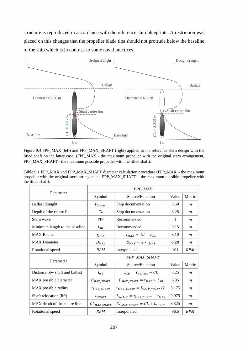
207
structure is reproduced in accordance with the reference ship blueprints. A restriction was
placed on this changes that the propeller blade tips should not protrude below the baseline
of the ship which is in contrast to some naval practices.
Design draught
Ballast
Base line
Shaft centre line
CL
= 3
.25
m
LBL
Design draught
Ballast
Base line
Shaft centre line
CL
= 3
.325
m
LBL
Diameter = 6.35 mDiameter = 6.20 m
Figure 9.4 FPP_MAX (left) and FPP_MAX_SHAFT (right) applied to the reference stern design with the lifted shaft on the latter case. (FPP_MAX - the maximum propeller with the original stern arrangement, FPP_MAX_SHAFT - the maximum possible propeller with the lifted shaft).
Table 9.1 FPP_MAX and FPP_MAX_SHAFT diameter calculation procedure (FPP_MAX – the maximum propeller with the original stern arrangement, FPP_MAX_SHAFT – the maximum possible propeller with the lifted shaft).
Parameter FPP_MAX
Symbol Source/Equation Value Metric
Ballast draught 𝑃𝑃𝐵𝐵𝑔𝑔𝑙𝑙𝑙𝑙𝑔𝑔𝑔𝑔𝐴𝐴 Ship documentation 6.50 𝑛𝑛
Depth of the centre line 𝐶𝐶𝐿𝐿 Ship documentation 3.25 𝑛𝑛
Stern wave 𝑆𝑆𝑊𝑊 Recommended 1 𝑛𝑛
Minimum length to the baseline 𝐿𝐿𝐵𝐵𝑊𝑊 Recommended 0.15 𝑛𝑛
MAX Radius 𝑡𝑡𝑀𝑀𝐴𝐴𝑋𝑋 𝑡𝑡𝑀𝑀𝐴𝐴𝑋𝑋 = 𝐶𝐶𝐿𝐿 – 𝐿𝐿𝐵𝐵𝑊𝑊 3.10 𝑛𝑛
MAX Diameter 𝐷𝐷𝑀𝑀𝐴𝐴𝑋𝑋 𝐷𝐷𝑀𝑀𝐴𝐴𝑋𝑋 = 2 ∗ 𝑡𝑡𝑀𝑀𝐴𝐴𝑋𝑋 6.20 𝑛𝑛
Rotational speed 𝐵𝐵𝑃𝑃𝑁𝑁 Interpolated 101 𝐵𝐵𝑃𝑃𝑁𝑁
Parameter FPP_MAX_SHAFT
Symbol Source/Equation Value Metric
Distance btw shaft and ballast 𝐿𝐿𝑆𝑆𝐵𝐵 𝐿𝐿𝑆𝑆𝐵𝐵 = 𝑃𝑃𝐵𝐵𝑔𝑔𝑙𝑙𝑙𝑙𝑔𝑔𝑔𝑔𝐴𝐴 − 𝐶𝐶𝐿𝐿 3.25 𝑛𝑛
MAX possible diameter 𝐷𝐷𝑀𝑀𝐴𝐴𝑋𝑋_𝑆𝑆𝐻𝐻𝐴𝐴𝐹𝐹𝑇𝑇 𝐷𝐷𝑀𝑀𝐴𝐴𝑋𝑋_𝑆𝑆𝐻𝐻𝐴𝐴𝐹𝐹𝑇𝑇 = 𝑡𝑡𝑀𝑀𝐴𝐴𝑋𝑋 + 𝐿𝐿𝑆𝑆𝐵𝐵 6.35 𝑛𝑛
MAX possible radius 𝑡𝑡𝑀𝑀𝐴𝐴𝑋𝑋_𝑆𝑆𝐻𝐻𝐴𝐴𝐹𝐹𝑇𝑇 𝑡𝑡𝑀𝑀𝐴𝐴𝑋𝑋_𝑆𝑆𝐻𝐻𝐴𝐴𝐹𝐹𝑇𝑇 = 𝐷𝐷𝑀𝑀𝐴𝐴𝑋𝑋_𝑆𝑆𝐻𝐻𝐴𝐴𝐹𝐹𝑇𝑇/2 3.175 𝑛𝑛
Shaft relocation (lift) 𝐿𝐿𝑆𝑆𝐻𝐻𝐴𝐴𝐹𝐹𝑇𝑇 𝐿𝐿𝑆𝑆𝐻𝐻𝐴𝐴𝐹𝐹𝑇𝑇 = 𝑡𝑡𝑀𝑀𝐴𝐴𝑋𝑋_𝑆𝑆𝐻𝐻𝐴𝐴𝐹𝐹𝑇𝑇 − 𝑡𝑡𝑀𝑀𝐴𝐴𝑋𝑋 0.075 𝑛𝑛
MAX depth of the centre line 𝐶𝐶𝐿𝐿𝑀𝑀𝐴𝐴𝑋𝑋_𝑆𝑆𝐻𝐻𝐴𝐴𝐹𝐹𝑇𝑇 𝐶𝐶𝐿𝐿𝑀𝑀𝐴𝐴𝑋𝑋_𝑆𝑆𝐻𝐻𝐴𝐴𝐹𝐹𝑇𝑇 = 𝐶𝐶𝐿𝐿 + 𝐿𝐿𝑆𝑆𝐻𝐻𝐴𝐴𝐹𝐹𝑇𝑇 3.325 𝑛𝑛
Rotational speed 𝐵𝐵𝑃𝑃𝑁𝑁 Interpolated 96.5 𝐵𝐵𝑃𝑃𝑁𝑁
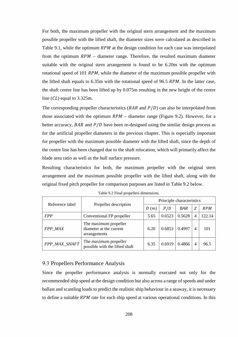
208
For both, the maximum propeller with the original stern arrangement and the maximum
possible propeller with the lifted shaft, the diameter sizes were calculated as described in
Table 9.1, while the optimum 𝐵𝐵𝑃𝑃𝑁𝑁 at the design condition for each case was interpolated
from the optimum 𝐵𝐵𝑃𝑃𝑁𝑁 – diameter range. Therefore, the resulted maximum diameter
suitable with the original stern arrangement is found to be 6.20m with the optimum
rotational speed of 101 𝐵𝐵𝑃𝑃𝑁𝑁, while the diameter of the maximum possible propeller with
the lifted shaft equals to 6.35m with the rotational speed of 96.5 𝐵𝐵𝑃𝑃𝑁𝑁. In the latter case,
the shaft centre line has been lifted up by 0.075m resulting in the new height of the centre
line (𝐶𝐶𝐿𝐿) equal to 3.325m.
The corresponding propeller characteristics (𝐵𝐵𝐵𝐵𝐵𝐵 and 𝑃𝑃/𝐷𝐷) can also be interpolated from
those associated with the optimum 𝐵𝐵𝑃𝑃𝑁𝑁 – diameter range (Figure 9.2). However, for a
better accuracy, 𝐵𝐵𝐵𝐵𝐵𝐵 and 𝑃𝑃/𝐷𝐷 have been re-designed using the similar design process as
for the artificial propeller diameters in the previous chapter. This is especially important
for propeller with the maximum possible diameter with the lifted shaft, since the depth of
the centre line has been changed due to the shaft relocation, which will primarily affect the
blade area ratio as well as the hull surface pressure.
Resulting characteristics for both, the maximum propeller with the original stern
arrangement and the maximum possible propeller with the lifted shaft, along with the
original fixed pitch propeller for comparison purposes are listed in Table 9.2 below.
Table 9.2 Final propellers dimensions.
Reference label Propeller description Principle characteristics
𝐷𝐷 (𝑛𝑛) 𝑃𝑃/𝐷𝐷 BAR 𝑍𝑍 𝐵𝐵𝑃𝑃𝑁𝑁 FPP Conventional FP propeller 5.65 0.6523 0.5628 4 122.14
FPP_MAX The maximum propeller diameter at the current arrangements
6.20 0.6853 0.4997 4 101
FPP_MAX_SHAFT The maximum propeller possible with the lifted shaft 6.35 0.6919 0.4866 4 96.5
Propellers Performance Analysis Since the propeller performance analysis is normally executed not only for the
recommended ship speed at the design condition but also across a range of speeds and under
ballast and scantling loads to predict the realistic ship behaviour in a seaway, it is necessary
to define a suitable 𝐵𝐵𝑃𝑃𝑁𝑁 rate for each ship speed at various operational conditions. In this
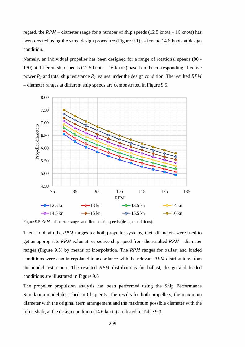
209
regard, the 𝐵𝐵𝑃𝑃𝑁𝑁 – diameter range for a number of ship speeds (12.5 knots – 16 knots) has
been created using the same design procedure (Figure 9.1) as for the 14.6 knots at design
condition.
Namely, an individual propeller has been designed for a range of rotational speeds (80 -
130) at different ship speeds (12.5 knots – 16 knots) based on the corresponding effective
power 𝑃𝑃𝐸𝐸 and total ship resistance 𝐵𝐵𝑇𝑇 values under the design condition. The resulted 𝐵𝐵𝑃𝑃𝑁𝑁
– diameter ranges at different ship speeds are demonstrated in Figure 9.5.
Figure 9.5 𝐵𝐵𝑃𝑃𝑁𝑁 – diameter ranges at different ship speeds (design conditions).
Then, to obtain the 𝐵𝐵𝑃𝑃𝑁𝑁 ranges for both propeller systems, their diameters were used to
get an appropriate 𝐵𝐵𝑃𝑃𝑁𝑁 value at respective ship speed from the resulted 𝐵𝐵𝑃𝑃𝑁𝑁 – diameter
ranges (Figure 9.5) by means of interpolation. The 𝐵𝐵𝑃𝑃𝑁𝑁 ranges for ballast and loaded
conditions were also interpolated in accordance with the relevant 𝐵𝐵𝑃𝑃𝑁𝑁 distributions from
the model test report. The resulted 𝐵𝐵𝑃𝑃𝑁𝑁 distributions for ballast, design and loaded
conditions are illustrated in Figure 9.6
The propeller propulsion analysis has been performed using the Ship Performance
Simulation model described in Chapter 5. The results for both propellers, the maximum
diameter with the original stern arrangement and the maximum possible diameter with the
lifted shaft, at the design condition (14.6 knots) are listed in Table 9.3.
4.50
5.00
5.50
6.00
6.50
7.00
7.50
8.00
75 85 95 105 115 125 135
Prop
elle
r dia
met
ers
RPM12.5 kn 13 kn 13.5 kn 14 kn
14.5 kn 15 kn 15.5 kn 16 kn
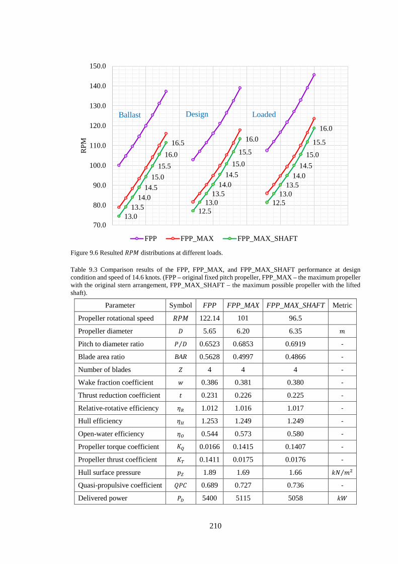
210
Figure 9.6 Resulted 𝐵𝐵𝑃𝑃𝑁𝑁 distributions at different loads.
Table 9.3 Comparison results of the FPP, FPP_MAX, and FPP_MAX_SHAFT performance at design condition and speed of 14.6 knots. (FPP – original fixed pitch propeller, FPP_MAX – the maximum propeller with the original stern arrangement, FPP_MAX_SHAFT – the maximum possible propeller with the lifted shaft).
Parameter Symbol FPP FPP_MAX FPP_MAX_SHAFT Metric
Propeller rotational speed 𝐵𝐵𝑃𝑃𝑁𝑁 122.14 101 96.5
Propeller diameter 𝐷𝐷 5.65 6.20 6.35 𝑛𝑛
Pitch to diameter ratio 𝑃𝑃 𝐷𝐷⁄ 0.6523 0.6853 0.6919 -
Blade area ratio BAR 0.5628 0.4997 0.4866 -
Number of blades 𝑍𝑍 4 4 4 -
Wake fraction coefficient 𝑤𝑤 0.386 0.381 0.380 -
Thrust reduction coefficient 𝐶𝐶 0.231 0.226 0.225 -
Relative-rotative efficiency 𝜂𝜂𝑅𝑅 1.012 1.016 1.017 -
Hull efficiency 𝜂𝜂𝐻𝐻 1.253 1.249 1.249 -
Open-water efficiency 𝜂𝜂𝑂𝑂 0.544 0.573 0.580 -
Propeller torque coefficient 𝐾𝐾𝑄𝑄 0.0166 0.1415 0.1407 -
Propeller thrust coefficient 𝐾𝐾𝑇𝑇 0.1411 0.0175 0.0176 -
Hull surface pressure 𝐶𝐶𝑍𝑍 1.89 1.69 1.66 𝑘𝑘𝑁𝑁 𝑛𝑛2⁄
Quasi-propulsive coefficient 𝑄𝑄𝑃𝑃𝐶𝐶 0.689 0.727 0.736 -
Delivered power 𝑃𝑃𝐷𝐷 5400 5115 5058 𝑘𝑘𝑊𝑊
13.013.5
14.014.5
15.015.5
16.016.5
12.513.0
13.514.0
14.515.0
15.5
16.0
12.513.0
13.514.0
14.515.0
15.5
16.0
70.0
80.0
90.0
100.0
110.0
120.0
130.0
140.0
150.0
RPM
FPP FPP_MAX FPP_MAX_SHAFT
Ballast Design Loaded
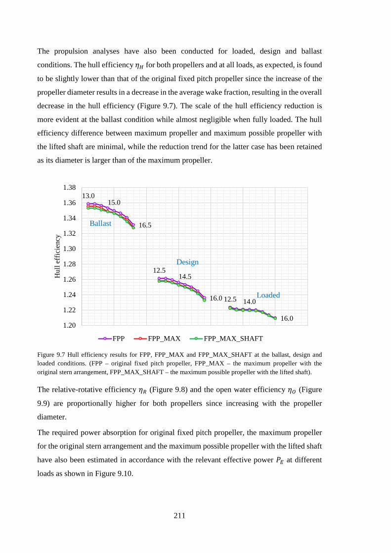
211
The propulsion analyses have also been conducted for loaded, design and ballast
conditions. The hull efficiency 𝜂𝜂𝐻𝐻 for both propellers and at all loads, as expected, is found
to be slightly lower than that of the original fixed pitch propeller since the increase of the
propeller diameter results in a decrease in the average wake fraction, resulting in the overall
decrease in the hull efficiency (Figure 9.7). The scale of the hull efficiency reduction is
more evident at the ballast condition while almost negligible when fully loaded. The hull
efficiency difference between maximum propeller and maximum possible propeller with
the lifted shaft are minimal, while the reduction trend for the latter case has been retained
as its diameter is larger than of the maximum propeller.
Figure 9.7 Hull efficiency results for FPP, FPP_MAX and FPP_MAX_SHAFT at the ballast, design and loaded conditions. (FPP – original fixed pitch propeller, FPP_MAX – the maximum propeller with the original stern arrangement, FPP_MAX_SHAFT – the maximum possible propeller with the lifted shaft).
The relative-rotative efficiency 𝜂𝜂𝑅𝑅 (Figure 9.8) and the open water efficiency 𝜂𝜂𝑂𝑂 (Figure
9.9) are proportionally higher for both propellers since increasing with the propeller
diameter.
The required power absorption for original fixed pitch propeller, the maximum propeller
for the original stern arrangement and the maximum possible propeller with the lifted shaft
have also been estimated in accordance with the relevant effective power 𝑃𝑃𝐸𝐸 at different
loads as shown in Figure 9.10.
13.015.0
16.5
12.514.5
16.0 12.5 14.0
16.01.20
1.22
1.24
1.26
1.28
1.30
1.32
1.34
1.36
1.38
Hul
l eff
icie
ncy
FPP FPP_MAX FPP_MAX_SHAFT
Ballast
Design
Loaded
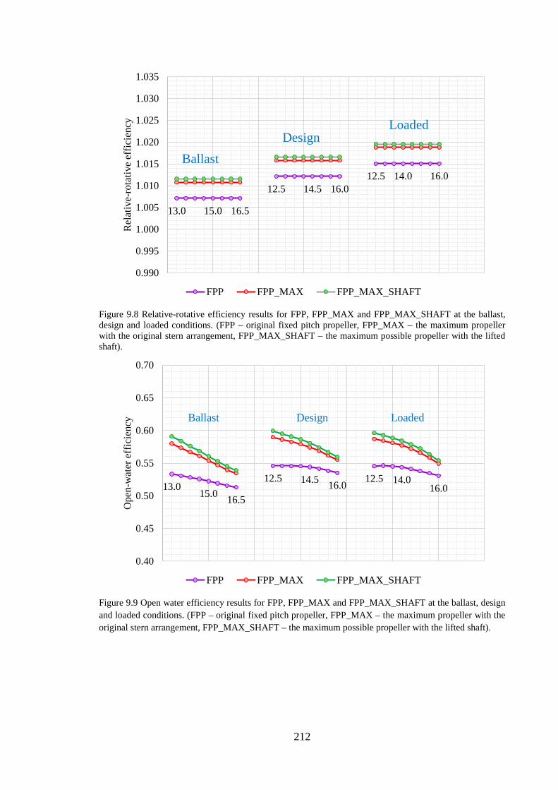
212
Figure 9.8 Relative-rotative efficiency results for FPP, FPP_MAX and FPP_MAX_SHAFT at the ballast, design and loaded conditions. (FPP – original fixed pitch propeller, FPP_MAX – the maximum propeller with the original stern arrangement, FPP_MAX_SHAFT – the maximum possible propeller with the lifted shaft).
Figure 9.9 Open water efficiency results for FPP, FPP_MAX and FPP_MAX_SHAFT at the ballast, design and loaded conditions. (FPP – original fixed pitch propeller, FPP_MAX – the maximum propeller with the original stern arrangement, FPP_MAX_SHAFT – the maximum possible propeller with the lifted shaft).
13.0 15.0 16.5
12.5 14.5 16.012.5 14.0 16.0
0.990
0.995
1.000
1.005
1.010
1.015
1.020
1.025
1.030
1.035
Rel
ativ
e-ro
tativ
e ef
ficie
ncy
FPP FPP_MAX FPP_MAX_SHAFT
BallastDesign
Loaded
13.015.0 16.5
12.5 14.5 16.0 12.5 14.016.0
0.40
0.45
0.50
0.55
0.60
0.65
0.70
Ope
n-w
ater
eff
icie
ncy
FPP FPP_MAX FPP_MAX_SHAFT
Ballast Design Loaded
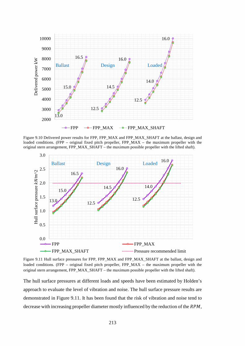
213
Figure 9.10 Delivered power results for FPP, FPP_MAX and FPP_MAX_SHAFT at the ballast, design and loaded conditions. (FPP – original fixed pitch propeller, FPP_MAX – the maximum propeller with the original stern arrangement, FPP_MAX_SHAFT – the maximum possible propeller with the lifted shaft).
Figure 9.11 Hull surface pressures for FPP, FPP_MAX and FPP_MAX_SHAFT at the ballast, design and loaded conditions. (FPP – original fixed pitch propeller, FPP_MAX – the maximum propeller with the original stern arrangement, FPP_MAX_SHAFT – the maximum possible propeller with the lifted shaft).
The hull surface pressures at different loads and speeds have been estimated by Holden’s
approach to evaluate the level of vibration and noise. The hull surface pressure results are
demonstrated in Figure 9.11. It has been found that the risk of vibration and noise tend to
decrease with increasing propeller diameter mostly influenced by the reduction of the 𝐵𝐵𝑃𝑃𝑁𝑁,
13.0
15.0
16.5
12.5
14.5
16.0
12.5
14.0
16.0
2000
3000
4000
5000
6000
7000
8000
9000
10000D
eliv
ered
pow
er k
W
FPP FPP_MAX FPP_MAX_SHAFT
Ballast Design Loaded
13.0
15.0
16.5
12.5
14.5
16.0
12.5
14.0
16.0
0.0
0.5
1.0
1.5
2.0
2.5
3.0
Hul
l sur
face
pre
ssur
e 𝑘𝑘𝑁𝑁
∕𝑛𝑛^2
FPP FPP_MAXFPP_MAX_SHAFT Pressure recommended limit
Ballast Design Loaded
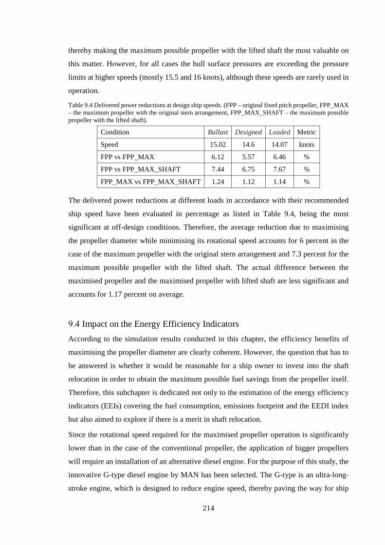
214
thereby making the maximum possible propeller with the lifted shaft the most valuable on
this matter. However, for all cases the hull surface pressures are exceeding the pressure
limits at higher speeds (mostly 15.5 and 16 knots), although these speeds are rarely used in
operation.
Table 9.4 Delivered power reductions at design ship speeds. (FPP – original fixed pitch propeller, FPP_MAX – the maximum propeller with the original stern arrangement, FPP_MAX_SHAFT – the maximum possible propeller with the lifted shaft).
Condition Ballast Designed Loaded Metric
Speed 15.02 14.6 14.07 knots
FPP vs FPP_MAX 6.12 5.57 6.46 %
FPP vs FPP_MAX_SHAFT 7.44 6.75 7.67 %
FPP_MAX vs FPP_MAX_SHAFT 1.24 1.12 1.14 %
The delivered power reductions at different loads in accordance with their recommended
ship speed have been evaluated in percentage as listed in Table 9.4, being the most
significant at off-design conditions. Therefore, the average reduction due to maximising
the propeller diameter while minimising its rotational speed accounts for 6 percent in the
case of the maximum propeller with the original stern arrangement and 7.3 percent for the
maximum possible propeller with the lifted shaft. The actual difference between the
maximised propeller and the maximised propeller with lifted shaft are less significant and
accounts for 1.17 percent on average.
Impact on the Energy Efficiency Indicators According to the simulation results conducted in this chapter, the efficiency benefits of
maximising the propeller diameter are clearly coherent. However, the question that has to
be answered is whether it would be reasonable for a ship owner to invest into the shaft
relocation in order to obtain the maximum possible fuel savings from the propeller itself.
Therefore, this subchapter is dedicated not only to the estimation of the energy efficiency
indicators (EEIs) covering the fuel consumption, emissions footprint and the EEDI index
but also aimed to explore if there is a merit in shaft relocation.
Since the rotational speed required for the maximised propeller operation is significantly
lower than in the case of the conventional propeller, the application of bigger propellers
will require an installation of an alternative diesel engine. For the purpose of this study, the
innovative G-type diesel engine by MAN has been selected. The G-type is an ultra-long-
stroke engine, which is designed to reduce engine speed, thereby paving the way for ship
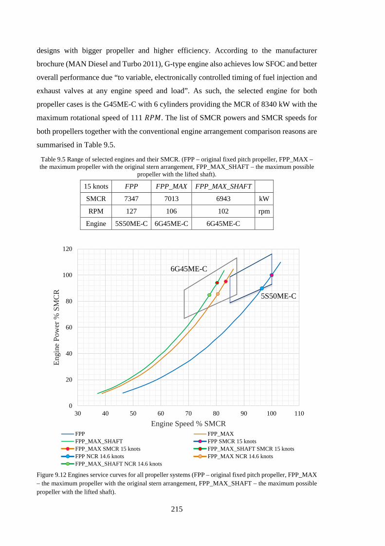
215
designs with bigger propeller and higher efficiency. According to the manufacturer
brochure (MAN Diesel and Turbo 2011), G-type engine also achieves low SFOC and better
overall performance due “to variable, electronically controlled timing of fuel injection and
exhaust valves at any engine speed and load”. As such, the selected engine for both
propeller cases is the G45ME-C with 6 cylinders providing the MCR of 8340 kW with the
maximum rotational speed of 111 𝐵𝐵𝑃𝑃𝑁𝑁. The list of SMCR powers and SMCR speeds for
both propellers together with the conventional engine arrangement comparison reasons are
summarised in Table 9.5.
Table 9.5 Range of selected engines and their SMCR. (FPP – original fixed pitch propeller, FPP_MAX – the maximum propeller with the original stern arrangement, FPP_MAX_SHAFT – the maximum possible
propeller with the lifted shaft).
15 knots FPP FPP_MAX FPP_MAX_SHAFT
SMCR 7347 7013 6943 kW
RPM 127 106 102 rpm
Engine 5S50ME-C 6G45ME-C 6G45ME-C
Figure 9.12 Engines service curves for all propeller systems (FPP – original fixed pitch propeller, FPP_MAX – the maximum propeller with the original stern arrangement, FPP_MAX_SHAFT – the maximum possible propeller with the lifted shaft).
0
20
40
60
80
100
120
30 40 50 60 70 80 90 100 110
Engi
ne P
ower
% S
MC
R
Engine Speed % SMCRFPP FPP_MAXFPP_MAX_SHAFT FPP SMCR 15 knotsFPP_MAX SMCR 15 knots FPP_MAX_SHAFT SMCR 15 knotsFPP NCR 14.6 knots FPP_MAX NCR 14.6 knotsFPP_MAX_SHAFT NCR 14.6 knots
5S50ME-C
6G45ME-C
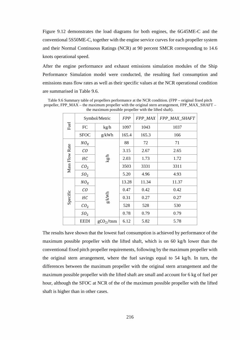
216
Figure 9.12 demonstrates the load diagrams for both engines, the 6G45ME-C and the
conventional 5S50ME-C, together with the engine service curves for each propeller system
and their Normal Continuous Ratings (NCR) at 90 percent SMCR corresponding to 14.6
knots operational speed.
After the engine performance and exhaust emissions simulation modules of the Ship
Performance Simulation model were conducted, the resulting fuel consumption and
emissions mass flow rates as well as their specific values at the NCR operational condition
are summarised in Table 9.6.
Table 9.6 Summary table of propellers performance at the NCR condition. (FPP – original fixed pitch propeller, FPP_MAX – the maximum propeller with the original stern arrangement, FPP_MAX_SHAFT –
the maximum possible propeller with the lifted shaft).
Fuel
Symbol/Metric FPP FPP_MAX FPP_MAX_SHAFT
FC kg/h 1097 1043 1037
SFOC g/kWh 165.4 165.3 166
Mas
s Flo
w R
ate 𝑁𝑁𝐶𝐶𝑋𝑋
kg/h
88 72 71
𝐶𝐶𝐶𝐶 3.15 2.67 2.65
𝐻𝐻𝐶𝐶 2.03 1.73 1.72
𝐶𝐶𝐶𝐶2 3503 3331 3311
𝑆𝑆𝐶𝐶2 5.20 4.96 4.93
Spec
ific
𝑁𝑁𝐶𝐶𝑋𝑋
g/kW
h
13.28 11.34 11.37
𝐶𝐶𝐶𝐶 0.47 0.42 0.42
𝐻𝐻𝐶𝐶 0.31 0.27 0.27
𝐶𝐶𝐶𝐶2 528 528 530
𝑆𝑆𝐶𝐶2 0.78 0.79 0.79
EEDI gCO2/tnm 6.12 5.82 5.78
The results have shown that the lowest fuel consumption is achieved by performance of the
maximum possible propeller with the lifted shaft, which is on 60 kg/h lower than the
conventional fixed pitch propeller requirements, following by the maximum propeller with
the original stern arrangement, where the fuel savings equal to 54 kg/h. In turn, the
differences between the maximum propeller with the original stern arrangement and the
maximum possible propeller with the lifted shaft are small and account for 6 kg of fuel per
hour, although the SFOC at NCR of the of the maximum possible propeller with the lifted
shaft is higher than in other cases.
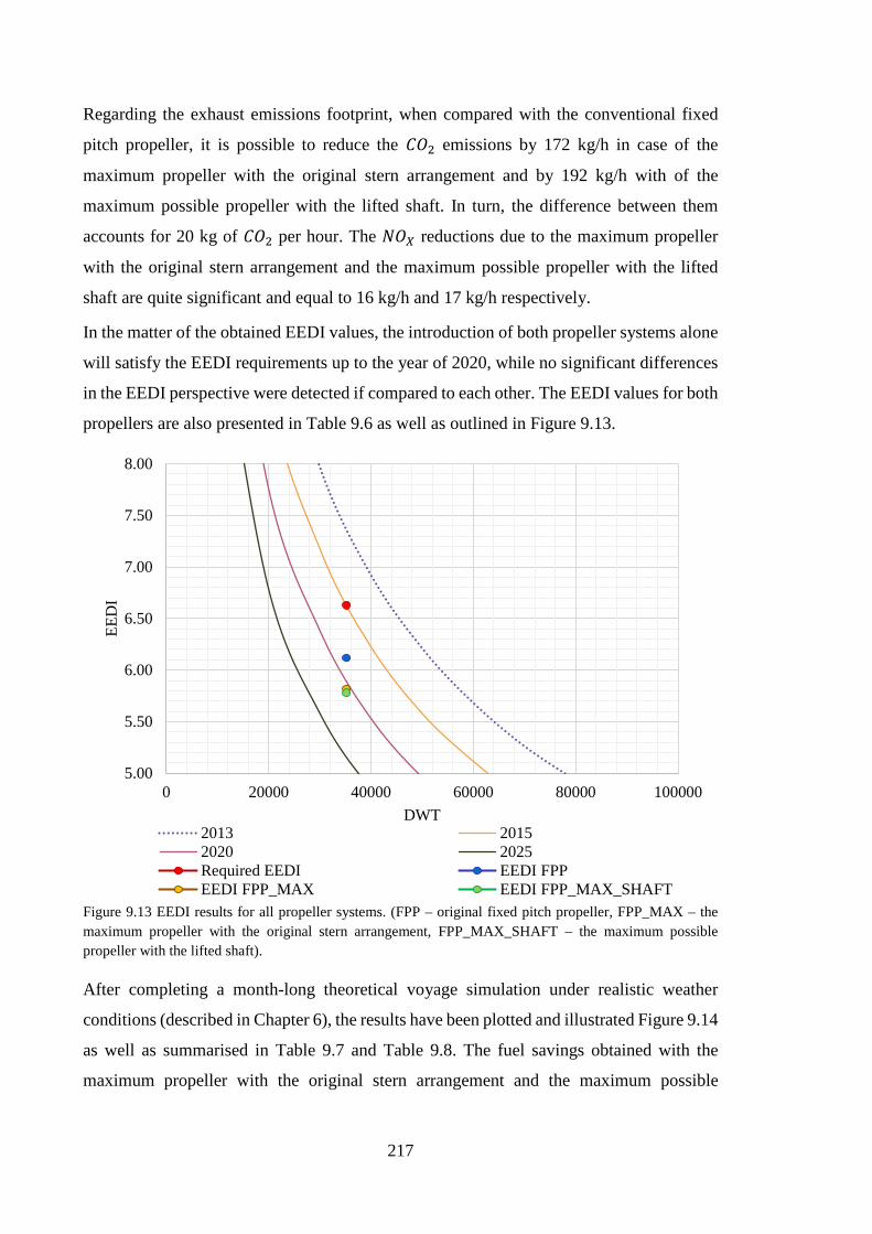
217
Regarding the exhaust emissions footprint, when compared with the conventional fixed
pitch propeller, it is possible to reduce the 𝐶𝐶𝐶𝐶2 emissions by 172 kg/h in case of the
maximum propeller with the original stern arrangement and by 192 kg/h with of the
maximum possible propeller with the lifted shaft. In turn, the difference between them
accounts for 20 kg of 𝐶𝐶𝐶𝐶2 per hour. The 𝑁𝑁𝐶𝐶𝑋𝑋 reductions due to the maximum propeller
with the original stern arrangement and the maximum possible propeller with the lifted
shaft are quite significant and equal to 16 kg/h and 17 kg/h respectively.
In the matter of the obtained EEDI values, the introduction of both propeller systems alone
will satisfy the EEDI requirements up to the year of 2020, while no significant differences
in the EEDI perspective were detected if compared to each other. The EEDI values for both
propellers are also presented in Table 9.6 as well as outlined in Figure 9.13.
Figure 9.13 EEDI results for all propeller systems. (FPP – original fixed pitch propeller, FPP_MAX – the maximum propeller with the original stern arrangement, FPP_MAX_SHAFT – the maximum possible propeller with the lifted shaft).
After completing a month-long theoretical voyage simulation under realistic weather
conditions (described in Chapter 6), the results have been plotted and illustrated Figure 9.14
as well as summarised in Table 9.7 and Table 9.8. The fuel savings obtained with the
maximum propeller with the original stern arrangement and the maximum possible
5.00
5.50
6.00
6.50
7.00
7.50
8.00
0 20000 40000 60000 80000 100000
EED
I
DWT2013 20152020 2025Required EEDI EEDI FPPEEDI FPP_MAX EEDI FPP_MAX_SHAFT
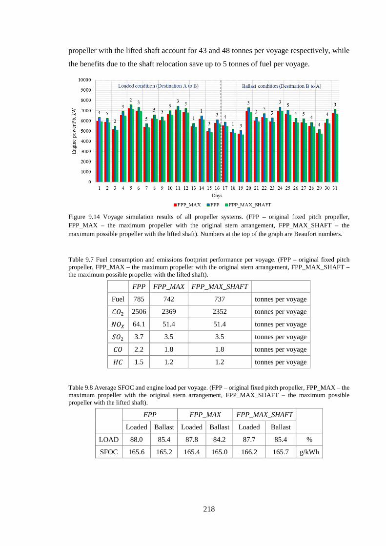
218
propeller with the lifted shaft account for 43 and 48 tonnes per voyage respectively, while
the benefits due to the shaft relocation save up to 5 tonnes of fuel per voyage.
Figure 9.14 Voyage simulation results of all propeller systems. (FPP – original fixed pitch propeller, FPP_MAX – the maximum propeller with the original stern arrangement, FPP_MAX_SHAFT – the maximum possible propeller with the lifted shaft). Numbers at the top of the graph are Beaufort numbers.
Table 9.7 Fuel consumption and emissions footprint performance per voyage. (FPP – original fixed pitch propeller, FPP_MAX – the maximum propeller with the original stern arrangement, FPP_MAX_SHAFT – the maximum possible propeller with the lifted shaft).
FPP FPP_MAX FPP_MAX_SHAFT
Fuel 785 742 737 tonnes per voyage
𝐶𝐶𝐶𝐶2 2506 2369 2352 tonnes per voyage
𝑁𝑁𝐶𝐶𝑋𝑋 64.1 51.4 51.4 tonnes per voyage
𝑆𝑆𝐶𝐶2 3.7 3.5 3.5 tonnes per voyage
𝐶𝐶𝐶𝐶 2.2 1.8 1.8 tonnes per voyage
𝐻𝐻𝐶𝐶 1.5 1.2 1.2 tonnes per voyage
Table 9.8 Average SFOC and engine load per voyage. (FPP – original fixed pitch propeller, FPP_MAX – the maximum propeller with the original stern arrangement, FPP_MAX_SHAFT – the maximum possible propeller with the lifted shaft).
FPP FPP_MAX FPP_MAX_SHAFT
Loaded Ballast Loaded Ballast Loaded Ballast
LOAD 88.0 85.4 87.8 84.2 87.7 85.4 %
SFOC 165.6 165.2 165.4 165.0 166.2 165.7 g/kWh

219
As a final remark, in case if retrofitting, both, the maximum propeller with the original
stern arrangement and the maximum possible propeller with the lifted shaft systems will
require a significant financial effort to provide new propeller, super slow diesel engine as
well as to modify the transmission system for the latter case. However, for new builds,
maximising the propeller diameter is a good option to save up to 50 tonnes of fuel per
voyage and being especially profitable should fuel prices increase; again reduce the 𝐶𝐶𝐶𝐶2
emissions by almost 200 kg per hour and 𝑁𝑁𝐶𝐶𝑋𝑋 by 17 kg per hour while complying with the
EEDI index requirements up to 2020. In addition, there is no need for the shaft relocation
should the propeller size be confirmed prior the power plant selection making the
preliminary ship performance simulation an important part of the efficient ship design.
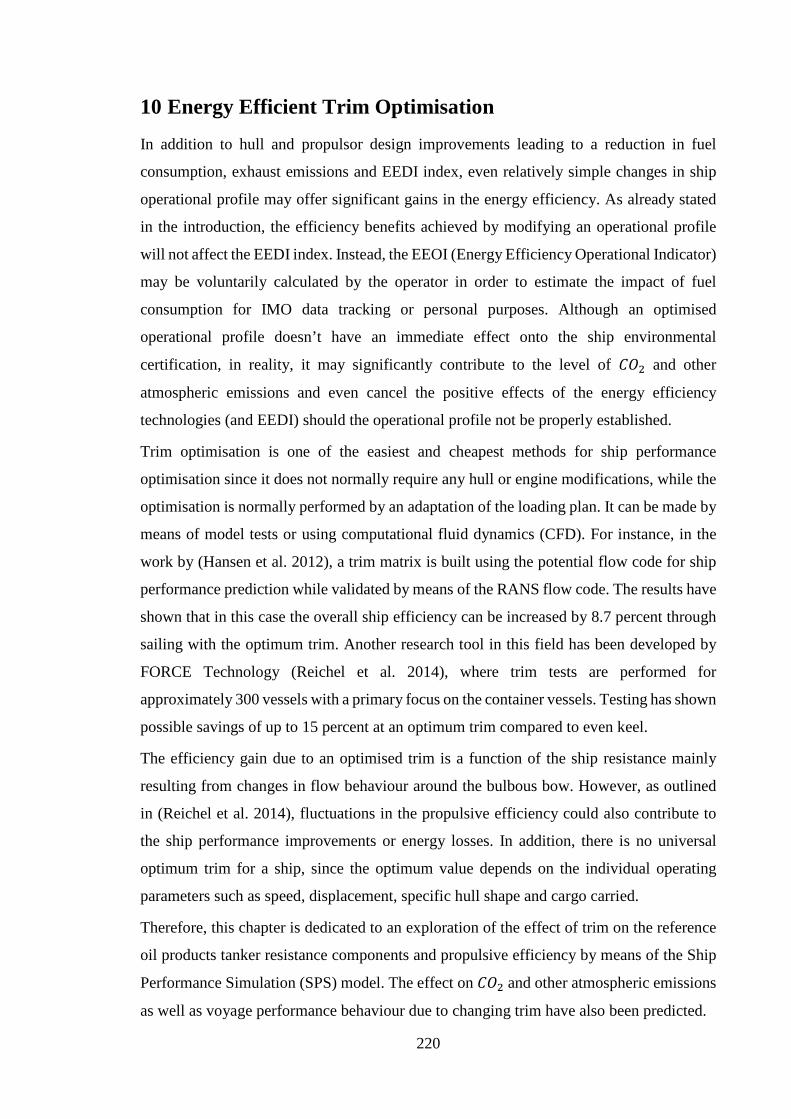
220
10 Energy Efficient Trim Optimisation
In addition to hull and propulsor design improvements leading to a reduction in fuel
consumption, exhaust emissions and EEDI index, even relatively simple changes in ship
operational profile may offer significant gains in the energy efficiency. As already stated
in the introduction, the efficiency benefits achieved by modifying an operational profile
will not affect the EEDI index. Instead, the EEOI (Energy Efficiency Operational Indicator)
may be voluntarily calculated by the operator in order to estimate the impact of fuel
consumption for IMO data tracking or personal purposes. Although an optimised
operational profile doesn’t have an immediate effect onto the ship environmental
certification, in reality, it may significantly contribute to the level of 𝐶𝐶𝐶𝐶2 and other
atmospheric emissions and even cancel the positive effects of the energy efficiency
technologies (and EEDI) should the operational profile not be properly established.
Trim optimisation is one of the easiest and cheapest methods for ship performance
optimisation since it does not normally require any hull or engine modifications, while the
optimisation is normally performed by an adaptation of the loading plan. It can be made by
means of model tests or using computational fluid dynamics (CFD). For instance, in the
work by (Hansen et al. 2012), a trim matrix is built using the potential flow code for ship
performance prediction while validated by means of the RANS flow code. The results have
shown that in this case the overall ship efficiency can be increased by 8.7 percent through
sailing with the optimum trim. Another research tool in this field has been developed by
FORCE Technology (Reichel et al. 2014), where trim tests are performed for
approximately 300 vessels with a primary focus on the container vessels. Testing has shown
possible savings of up to 15 percent at an optimum trim compared to even keel.
The efficiency gain due to an optimised trim is a function of the ship resistance mainly
resulting from changes in flow behaviour around the bulbous bow. However, as outlined
in (Reichel et al. 2014), fluctuations in the propulsive efficiency could also contribute to
the ship performance improvements or energy losses. In addition, there is no universal
optimum trim for a ship, since the optimum value depends on the individual operating
parameters such as speed, displacement, specific hull shape and cargo carried.
Therefore, this chapter is dedicated to an exploration of the effect of trim on the reference
oil products tanker resistance components and propulsive efficiency by means of the Ship
Performance Simulation (SPS) model. The effect on 𝐶𝐶𝐶𝐶2 and other atmospheric emissions
as well as voyage performance behaviour due to changing trim have also been predicted.
221
Trim Definition Generally, trim is defined as the difference between the draught at stern (𝑃𝑃𝐴𝐴) and the bow
draught (𝑃𝑃𝐹𝐹) (Reichel et al. 2014):
𝑃𝑃𝑡𝑡𝑖𝑖𝑛𝑛 = 𝑃𝑃𝐴𝐴 − 𝑃𝑃𝐹𝐹 10.1
Design Draught = 9.75 m
Partially Loaded = 8 mEVEN KEEL
TRIM = - 1.75 m TF = 9.75 mTA = 8 m
TF = 7 mTRIM = 1 mTA = 8 m
STERN BOW
STERN BOW
STERN BOW
Figure 10.1 Schematic representation of considered trim conditions.
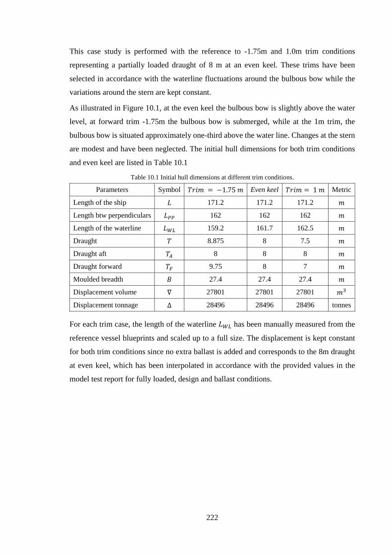
222
This case study is performed with the reference to -1.75m and 1.0m trim conditions
representing a partially loaded draught of 8 m at an even keel. These trims have been
selected in accordance with the waterline fluctuations around the bulbous bow while the
variations around the stern are kept constant.
As illustrated in Figure 10.1, at the even keel the bulbous bow is slightly above the water
level, at forward trim -1.75m the bulbous bow is submerged, while at the 1m trim, the
bulbous bow is situated approximately one-third above the water line. Changes at the stern
are modest and have been neglected. The initial hull dimensions for both trim conditions
and even keel are listed in Table 10.1
Table 10.1 Initial hull dimensions at different trim conditions.
Parameters Symbol 𝑃𝑃𝑡𝑡𝑖𝑖𝑛𝑛 = −1.75 𝑛𝑛 Even keel 𝑃𝑃𝑡𝑡𝑖𝑖𝑛𝑛 = 1 𝑛𝑛 Metric
Length of the ship 𝐿𝐿 171.2 171.2 171.2 𝑛𝑛
Length btw perpendiculars 𝐿𝐿𝑃𝑃𝑃𝑃 162 162 162 𝑛𝑛
Length of the waterline 𝐿𝐿𝑊𝑊𝑊𝑊 159.2 161.7 162.5 𝑛𝑛
Draught 𝑃𝑃 8.875 8 7.5 𝑛𝑛
Draught aft 𝑃𝑃𝐴𝐴 8 8 8 𝑛𝑛
Draught forward 𝑃𝑃𝐹𝐹 9.75 8 7 𝑛𝑛
Moulded breadth 𝐵𝐵 27.4 27.4 27.4 𝑛𝑛
Displacement volume ∇ 27801 27801 27801 𝑛𝑛3
Displacement tonnage ∆ 28496 28496 28496 tonnes
For each trim case, the length of the waterline 𝐿𝐿𝑊𝑊𝑊𝑊 has been manually measured from the
reference vessel blueprints and scaled up to a full size. The displacement is kept constant
for both trim conditions since no extra ballast is added and corresponds to the 8m draught
at even keel, which has been interpolated in accordance with the provided values in the
model test report for fully loaded, design and ballast conditions.
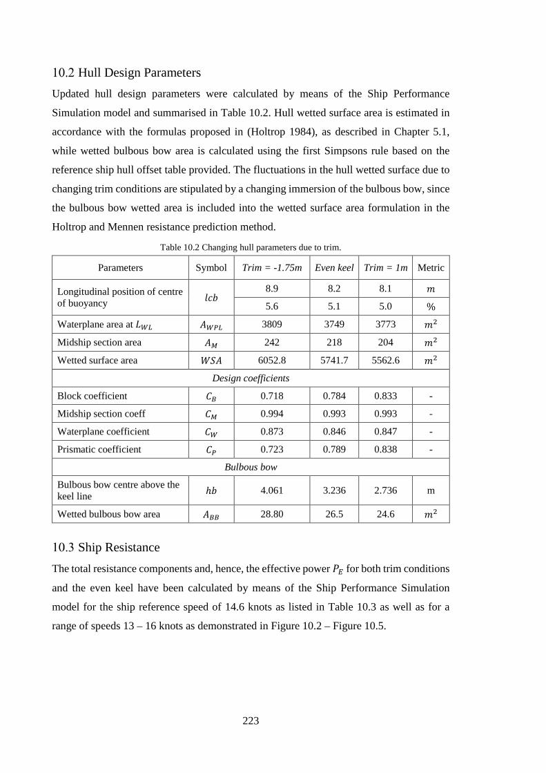
223
Hull Design Parameters Updated hull design parameters were calculated by means of the Ship Performance
Simulation model and summarised in Table 10.2. Hull wetted surface area is estimated in
accordance with the formulas proposed in (Holtrop 1984), as described in Chapter 5.1,
while wetted bulbous bow area is calculated using the first Simpsons rule based on the
reference ship hull offset table provided. The fluctuations in the hull wetted surface due to
changing trim conditions are stipulated by a changing immersion of the bulbous bow, since
the bulbous bow wetted area is included into the wetted surface area formulation in the
Holtrop and Mennen resistance prediction method.
Table 10.2 Changing hull parameters due to trim.
Parameters Symbol Trim = -1.75m Even keel Trim = 1m Metric
Longitudinal position of centre of buoyancy 𝑙𝑙𝐶𝐶𝑙𝑙
8.9 8.2 8.1 𝑛𝑛
5.6 5.1 5.0 %
Waterplane area at 𝐿𝐿𝑊𝑊𝑊𝑊 𝐵𝐵𝑊𝑊𝑃𝑃𝑊𝑊 3809 3749 3773 𝑛𝑛2
Midship section area 𝐵𝐵𝑀𝑀 242 218 204 𝑛𝑛2
Wetted surface area 𝑊𝑊𝑆𝑆𝐵𝐵 6052.8 5741.7 5562.6 𝑛𝑛2
Design coefficients
Block coefficient 𝐶𝐶𝐵𝐵 0.718 0.784 0.833 -
Midship section coeff 𝐶𝐶𝑀𝑀 0.994 0.993 0.993 -
Waterplane coefficient 𝐶𝐶𝑊𝑊 0.873 0.846 0.847 -
Prismatic coefficient 𝐶𝐶𝑃𝑃 0.723 0.789 0.838 -
Bulbous bow
Bulbous bow centre above the keel line ℎ𝑙𝑙 4.061 3.236 2.736 m
Wetted bulbous bow area 𝐵𝐵𝐵𝐵𝐵𝐵 28.80 26.5 24.6 𝑛𝑛2
Ship Resistance The total resistance components and, hence, the effective power 𝑃𝑃𝐸𝐸 for both trim conditions
and the even keel have been calculated by means of the Ship Performance Simulation
model for the ship reference speed of 14.6 knots as listed in Table 10.3 as well as for a
range of speeds 13 – 16 knots as demonstrated in Figure 10.2 – Figure 10.5.
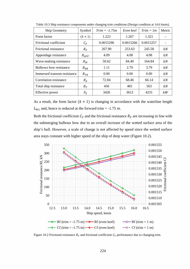
224
Table 10.3 Ship resistance components under changing trim conditions (Design condition at 14.6 knots).
Ship Geometry Symbol Trim = -1.75m Even keel Trim = 1m Metric
Form factor (𝑘𝑘 + 1) 1.223 1.267 1.321 -
Frictional coefficient 𝐶𝐶𝐹𝐹 0.0015296 0.0015266 0.0015257 -
Frictional resistance 𝐵𝐵𝐹𝐹 267.90 253.63 245.58 𝑘𝑘𝑁𝑁
Appendage resistance 𝐵𝐵𝐴𝐴𝑃𝑃𝑃𝑃 4.09 4.08 4.08 𝑘𝑘𝑁𝑁
Wave-making resistance 𝐵𝐵𝑊𝑊 50.62 84.40 164.84 𝑘𝑘𝑁𝑁
Bulbows bow resistance 𝐵𝐵𝐵𝐵𝐵𝐵 1.11 2.79 3.79 𝑘𝑘𝑁𝑁
Immersed transom resistance 𝐵𝐵𝑇𝑇𝑅𝑅 0.00 0.00 0.00 𝑘𝑘𝑁𝑁
Correlation resistance 𝐵𝐵𝐴𝐴 72.84 68.46 66.14 𝑘𝑘𝑁𝑁
Total ship resistance 𝐵𝐵𝑇𝑇 456 481 563 𝑘𝑘𝑁𝑁
Effective power 𝑃𝑃𝐸𝐸 3426 3612 4231 𝑘𝑘𝑊𝑊
As a result, the form factor (𝑘𝑘 + 1) is changing in accordance with the waterline length
𝐿𝐿𝑊𝑊𝑊𝑊 and, hence is reduced at the forward trim = -1.75 𝑛𝑛.
Both the frictional coefficient 𝐶𝐶𝐹𝐹 and the frictional resistance 𝐵𝐵𝐹𝐹 are increasing in line with
the submerging bulbous bow due to an overall increase of the wetted surface area of the
ship’s hull. However, a scale of change is not affected by speed since the wetted surface
area stays constant with higher speed of the ship of deep water (Figure 10.2).
Figure 10.2 Frictional resistance 𝐵𝐵𝐹𝐹 and frictional coefficient 𝐶𝐶𝐹𝐹 performance due to changing trim.
0.001505
0.001510
0.001515
0.001520
0.001525
0.001530
0.001535
0.001540
0.001545
0.001550
0.001555
0
50
100
150
200
250
300
350
12.5 13.0 13.5 14.0 14.5 15.0 15.5 16.0 16.5
Fric
tiona
l coe
ffic
ient
Cf
Fric
tiona
l res
ista
nce R
f, kN
Ship speed, knots
Rf (trim = -1.75 m) Rf (even keel) Rf (trim = 1 m)Cf (trim = -1.75 m) Cf (even keel) Cf (trim = 1 m)
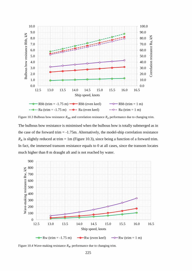
225
Figure 10.3 Bulbous bow resistance 𝐵𝐵𝐵𝐵𝐵𝐵 and correlation resistance 𝐵𝐵𝐴𝐴 performance due to changing trim.
The bulbous bow resistance is minimised when the bulbous bow is totally submerged as in
the case of the forward trim = -1.75m. Alternatively, the model-ship correlation resistance
𝐵𝐵𝐴𝐴 is slightly reduced at trim = 1m (Figure 10.3), since being a function of a forward trim.
In fact, the immersed transom resistance equals to 0 at all cases, since the transom locates
much higher than 8 m draught aft and is not reached by water.
Figure 10.4 Wave-making resistance 𝐵𝐵𝑊𝑊 performance due to changing trim.
0.0
10.0
20.0
30.0
40.0
50.0
60.0
70.0
80.0
90.0
100.0
0.0
1.0
2.0
3.0
4.0
5.0
6.0
7.0
8.0
9.0
10.0
12.5 13.0 13.5 14.0 14.5 15.0 15.5 16.0 16.5
Cor
rela
tion
resi
stan
ce R
a, k
N
Bul
bous
bow
resi
stan
ce R
bb, k
N
Ship speed, knots
Rbb (trim = -1.75 m) Rbb (even keel) Rbb (trim = 1 m)Ra (trim = -1.75 m) Ra (even keel) Ra (trim = 1 m)
0
100
200
300
400
500
600
700
800
900
12.5 13.0 13.5 14.0 14.5 15.0 15.5 16.0 16.5
Wav
e-m
akin
g re
sist
ance
Rw
, kN
Ship speed, knots
Rw (trim = -1.75 m) Rw (even keel) Rw (trim = 1 m)
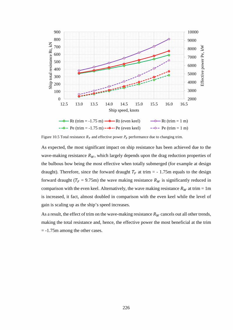
226
Figure 10.5 Total resistance 𝐵𝐵𝑇𝑇 and effective power 𝑃𝑃𝐸𝐸 performance due to changing trim.
As expected, the most significant impact on ship resistance has been achieved due to the
wave-making resistance 𝐵𝐵𝑊𝑊, which largely depends upon the drag reduction properties of
the bulbous bow being the most effective when totally submerged (for example at design
draught). Therefore, since the forward draught 𝑃𝑃𝐹𝐹 at trim = - 1.75m equals to the design
forward draught (𝑃𝑃𝐹𝐹 = 9.75m) the wave making resistance 𝐵𝐵𝑊𝑊 is significantly reduced in
comparison with the even keel. Alternatively, the wave making resistance 𝐵𝐵𝑊𝑊 at trim = 1m
is increased, it fact, almost doubled in comparison with the even keel while the level of
gain is scaling up as the ship’s speed increases.
As a result, the effect of trim on the wave-making resistance 𝐵𝐵𝑊𝑊 cancels out all other trends,
making the total resistance and, hence, the effective power the most beneficial at the trim
= -1.75m among the other cases.
2000
3000
4000
5000
6000
7000
8000
9000
10000
0
100
200
300
400
500
600
700
800
900
12.5 13.0 13.5 14.0 14.5 15.0 15.5 16.0 16.5
Effe
ctiv
e po
wer
Pe,
kW
Ship
tota
l res
ista
nce
Rt,
kN
Ship speed, knots
Rt (trim = -1.75 m) Rt (even keel) Rt (trim = 1 m)Pe (trim = -1.75 m) Pe (even keel) Pe (trim = 1 m)
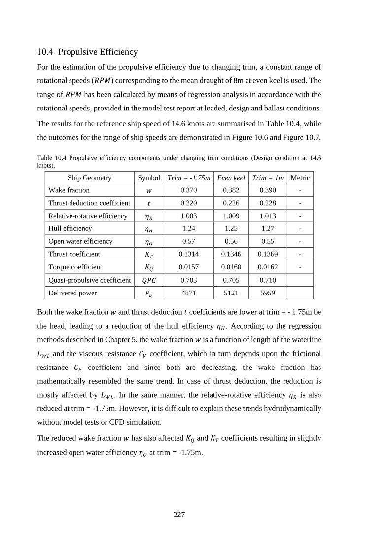
227
Propulsive Efficiency For the estimation of the propulsive efficiency due to changing trim, a constant range of
rotational speeds (𝐵𝐵𝑃𝑃𝑁𝑁) corresponding to the mean draught of 8m at even keel is used. The
range of 𝐵𝐵𝑃𝑃𝑁𝑁 has been calculated by means of regression analysis in accordance with the
rotational speeds, provided in the model test report at loaded, design and ballast conditions.
The results for the reference ship speed of 14.6 knots are summarised in Table 10.4, while
the outcomes for the range of ship speeds are demonstrated in Figure 10.6 and Figure 10.7.
Table 10.4 Propulsive efficiency components under changing trim conditions (Design condition at 14.6 knots).
Ship Geometry Symbol Trim = -1.75m Even keel Trim = 1m Metric
Wake fraction 𝑤𝑤 0.370 0.382 0.390 -
Thrust deduction coefficient 𝐶𝐶 0.220 0.226 0.228 -
Relative-rotative efficiency 𝜂𝜂𝑅𝑅 1.003 1.009 1.013 -
Hull efficiency 𝜂𝜂𝐻𝐻 1.24 1.25 1.27 -
Open water efficiency 𝜂𝜂𝑂𝑂 0.57 0.56 0.55 -
Thrust coefficient 𝐾𝐾𝑇𝑇 0.1314 0.1346 0.1369 -
Torque coefficient 𝐾𝐾𝑄𝑄 0.0157 0.0160 0.0162 -
Quasi-propulsive coefficient 𝑄𝑄𝑃𝑃𝐶𝐶 0.703 0.705 0.710
Delivered power 𝑃𝑃𝐷𝐷 4871 5121 5959
Both the wake fraction 𝑤𝑤 and thrust deduction 𝐶𝐶 coefficients are lower at trim = - 1.75m be
the head, leading to a reduction of the hull efficiency 𝜂𝜂𝐻𝐻. According to the regression
methods described in Chapter 5, the wake fraction 𝑤𝑤 is a function of length of the waterline
𝐿𝐿𝑊𝑊𝑊𝑊 and the viscous resistance 𝐶𝐶𝑉𝑉 coefficient, which in turn depends upon the frictional
resistance 𝐶𝐶𝐹𝐹 coefficient and since both are decreasing, the wake fraction has
mathematically resembled the same trend. In case of thrust deduction, the reduction is
mostly affected by 𝐿𝐿𝑊𝑊𝑊𝑊. In the same manner, the relative-rotative efficiency 𝜂𝜂𝑅𝑅 is also
reduced at trim = -1.75m. However, it is difficult to explain these trends hydrodynamically
without model tests or CFD simulation.
The reduced wake fraction 𝑤𝑤 has also affected 𝐾𝐾𝑄𝑄 and 𝐾𝐾𝑇𝑇 coefficients resulting in slightly
increased open water efficiency 𝜂𝜂𝑂𝑂 at trim = -1.75m.
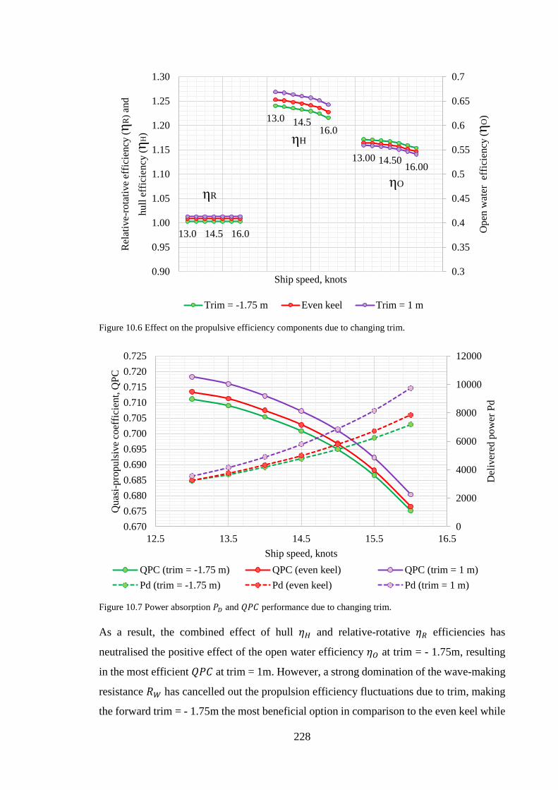
228
Figure 10.6 Effect on the propulsive efficiency components due to changing trim.
Figure 10.7 Power absorption 𝑃𝑃𝐷𝐷 and 𝑄𝑄𝑃𝑃𝐶𝐶 performance due to changing trim.
As a result, the combined effect of hull 𝜂𝜂𝐻𝐻 and relative-rotative 𝜂𝜂𝑅𝑅 efficiencies has
neutralised the positive effect of the open water efficiency 𝜂𝜂𝑂𝑂 at trim = - 1.75m, resulting
in the most efficient 𝑄𝑄𝑃𝑃𝐶𝐶 at trim = 1m. However, a strong domination of the wave-making
resistance 𝐵𝐵𝑊𝑊 has cancelled out the propulsion efficiency fluctuations due to trim, making
the forward trim = - 1.75m the most beneficial option in comparison to the even keel while
13.0 14.5 16.0
13.0 14.516.0
13.00 14.50 16.00
0.3
0.35
0.4
0.45
0.5
0.55
0.6
0.65
0.7
0.90
0.95
1.00
1.05
1.10
1.15
1.20
1.25
1.30
Ope
n w
ater
eff
icie
ncy
(ηO
)
Rel
ativ
e-ro
tativ
e ef
ficie
ncy
( ηR
) and
hull
effic
ienc
y ( η
H)
Ship speed, knots
Trim = -1.75 m Even keel Trim = 1 m
ηR
ηH
ηO
0
2000
4000
6000
8000
10000
12000
0.6700.6750.6800.6850.6900.6950.7000.7050.7100.7150.7200.725
12.5 13.5 14.5 15.5 16.5
Del
iver
ed p
ower
Pd
Qua
si-p
ropu
lsiv
e co
effic
ient
, QPC
Ship speed, knotsQPC (trim = -1.75 m) QPC (even keel) QPC (trim = 1 m)Pd (trim = -1.75 m) Pd (even keel) Pd (trim = 1 m)
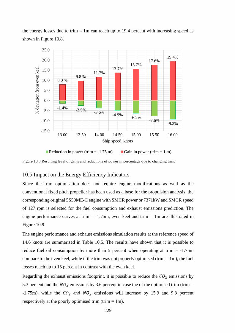
229
the energy losses due to trim = 1m can reach up to 19.4 percent with increasing speed as
shown in Figure 10.8.
Figure 10.8 Resulting level of gains and reductions of power in percentage due to changing trim.
Impact on the Energy Efficiency Indicators Since the trim optimisation does not require engine modifications as well as the
conventional fixed pitch propeller has been used as a base for the propulsion analysis, the
corresponding original 5S50ME-C engine with SMCR power or 7371kW and SMCR speed
of 127 rpm is selected for the fuel consumption and exhaust emissions prediction. The
engine performance curves at trim = -1.75m, even keel and trim = 1m are illustrated in
Figure 10.9.
The engine performance and exhaust emissions simulation results at the reference speed of
14.6 knots are summarised in Table 10.5. The results have shown that it is possible to
reduce fuel oil consumption by more than 5 percent when operating at trim = -1.75m
compare to the even keel, while if the trim was not properly optimised (trim = 1m), the fuel
losses reach up to 15 percent in contrast with the even keel.
Regarding the exhaust emissions footprint, it is possible to reduce the 𝐶𝐶𝐶𝐶2 emissions by
5.3 percent and the 𝑁𝑁𝐶𝐶𝑋𝑋 emissions by 3.6 percent in case the of the optimised trim (trim =
-1.75m), while the 𝐶𝐶𝐶𝐶2 and 𝑁𝑁𝐶𝐶𝑋𝑋 emissions will increase by 15.3 and 9.3 percent
respectively at the poorly optimised trim (trim = 1m).
-1.4% -2.5% -3.6% -4.9% -6.2% -7.6%-9.2%
8.0 %9.8 %
11.7%13.7%
15.7%17.6%
19.4%
-15.0
-10.0
-5.0
0.0
5.0
10.0
15.0
20.0
25.0
13.00 13.50 14.00 14.50 15.00 15.50 16.00
% d
evia
tion
from
eve
n ke
el
Ship speed, knots
Reduction in power (trim = -1.75 m) Gain in power (trim = 1.m)
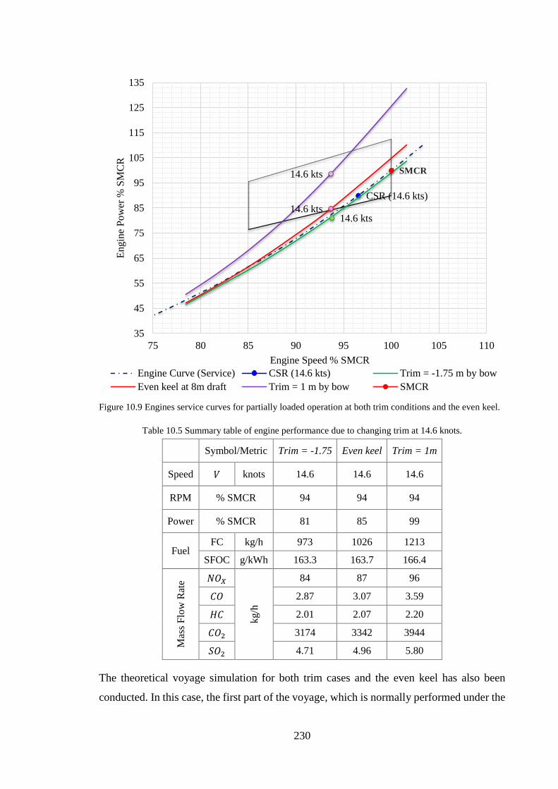
230
Figure 10.9 Engines service curves for partially loaded operation at both trim conditions and the even keel.
Table 10.5 Summary table of engine performance due to changing trim at 14.6 knots.
Symbol/Metric Trim = -1.75 Even keel Trim = 1m
Speed 𝑁𝑁 knots 14.6 14.6 14.6
RPM % SMCR 94 94 94
Power % SMCR 81 85 99
Fuel FC kg/h 973 1026 1213
SFOC g/kWh 163.3 163.7 166.4
Mas
s Flo
w R
ate 𝑁𝑁𝐶𝐶𝑋𝑋
kg/h
84 87 96
𝐶𝐶𝐶𝐶 2.87 3.07 3.59
𝐻𝐻𝐶𝐶 2.01 2.07 2.20
𝐶𝐶𝐶𝐶2 3174 3342 3944
𝑆𝑆𝐶𝐶2 4.71 4.96 5.80
The theoretical voyage simulation for both trim cases and the even keel has also been
conducted. In this case, the first part of the voyage, which is normally performed under the
CSR (14.6 kts)
14.6 kts14.6 kts
14.6 kts SMCR
35
45
55
65
75
85
95
105
115
125
135
75 80 85 90 95 100 105 110
Engi
ne P
ower
% S
MC
R
Engine Speed % SMCREngine Curve (Service) CSR (14.6 kts) Trim = -1.75 m by bowEven keel at 8m draft Trim = 1 m by bow SMCR
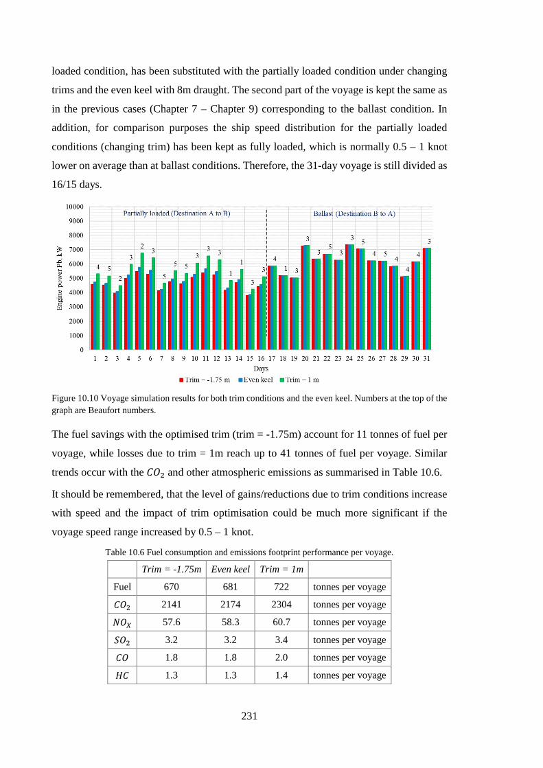
231
loaded condition, has been substituted with the partially loaded condition under changing
trims and the even keel with 8m draught. The second part of the voyage is kept the same as
in the previous cases (Chapter 7 – Chapter 9) corresponding to the ballast condition. In
addition, for comparison purposes the ship speed distribution for the partially loaded
conditions (changing trim) has been kept as fully loaded, which is normally 0.5 – 1 knot
lower on average than at ballast conditions. Therefore, the 31-day voyage is still divided as
16/15 days.
Figure 10.10 Voyage simulation results for both trim conditions and the even keel. Numbers at the top of the graph are Beaufort numbers.
The fuel savings with the optimised trim (trim = -1.75m) account for 11 tonnes of fuel per
voyage, while losses due to trim = 1m reach up to 41 tonnes of fuel per voyage. Similar
trends occur with the 𝐶𝐶𝐶𝐶2 and other atmospheric emissions as summarised in Table 10.6.
It should be remembered, that the level of gains/reductions due to trim conditions increase
with speed and the impact of trim optimisation could be much more significant if the
voyage speed range increased by 0.5 – 1 knot.
Table 10.6 Fuel consumption and emissions footprint performance per voyage.
Trim = -1.75m Even keel Trim = 1m
Fuel 670 681 722 tonnes per voyage
𝐶𝐶𝐶𝐶2 2141 2174 2304 tonnes per voyage
𝑁𝑁𝐶𝐶𝑋𝑋 57.6 58.3 60.7 tonnes per voyage
𝑆𝑆𝐶𝐶2 3.2 3.2 3.4 tonnes per voyage
𝐶𝐶𝐶𝐶 1.8 1.8 2.0 tonnes per voyage
𝐻𝐻𝐶𝐶 1.3 1.3 1.4 tonnes per voyage

232
Table 10.7 Average SFOC and engine load per voyage.
Trim = 1.75m Even keel Trim = 1m
Loaded Ballast Loaded Ballast Loaded Ballast
LOAD 63.7 84.8 66.0 84.8 74.8 84.8 %
SFOC 164.7 165.2 164.5 165.2 164.5 165.2 g/kWh
In Table 10.7, the average engine load and SFOC for both trim conditions and the even
keel are summarised. Indeed, the SFOC of trim = -1.75m is slightly higher due to low load.
Thus, in order to achieve the most efficient operation, the average ship speed could be
slightly increased to operate at about 70 percent load corresponding to the lowest fuel
consumption rate for this type of engine.
In conclusion, the results have shown that the impact of trim on ship efficiency is significant
and, if not optimised properly, can lead to serious power losses, while minimising the
benefits of energy saving devices and high-efficiency propellers as well as the initial
purpose of the EEDI certification.
On the other end of the spectrum, the trim optimisation is difficult to be controlled
governmentally, since it has to be performed in each individual case depending on load,
speed and the hull structure as well as the master’s discretion. However, the industry’s
interests in fuel savings and environmental concerns regarding the exhaust emissions
control coupled with the growing trim optimisation CFD based software development
could lead to some additional improvements addressed to the EEDI legislation, namely to
include the trim optimisation software installation as a mandatory requirement to a ship
owner in order to be issued with the EEDI certificate.

233
11 Future Hybrid Propulsion Concepts
By following the discussions in Chapter 2.5, progressive developments in battery and fuel
cell technologies as well as hybridisation and complete electrification of a number of
smaller ferries and offshore vessels hold a significant promise for more efficient use of
propulsion power coupled with the potential reductions in the atmospheric emissions for
larger vessels travelling longer distances.
Since, in the case of modern marine diesel engines the energy efficiency and specific
emissions depend upon the load, being less beneficial at low and changing loads. The
hybrid-based operational profile can help to avoid the operation at these loads by using a
battery bank to store the excess energy produced due to load variations and then return it
to the system when needed while operating at constant load and potentially producing some
extra power by means of renewable energy sources or fuel cells. Such an operational
principle is often referred as a load leveling (Whitelegg & Bucknall 2013) or peak-shaving
(Pestana 2014).
The benefit of hybrid-based power systems is closely associated with the operational profile
and type of vessel. Traditionally, load leveling operational concepts are considered to be
especially advantageous when the level of load fluctuations is high, for instance for tugs,
vessels based on the dynamic positioning (DP) operations as well as offshore supply
vessels. A typical example is the first hybrid offshore supply vessel, Viking Lady, built in
2013 with incorporated fuel cell technology as a part of the propulsion system. According
to various industry references, this system provides the primary benefits of 20 percent in
reduction of fuel consumption, 𝐶𝐶𝐶𝐶2 and other atmospheric emissions. However, there is a
number of other operational profiles where the frequency and level of load fluctuations is
less obvious but undervalued, including the additional fuel consumption due to heavy
weather conditions influenced by increased wave-making resistance and fluctuating
propeller immersion.
Based on the initial service data and voyage simulation results of the Ship Performance
Simulation model, the engine load of the reference oil products tanker is also fluctuating
due to changing weather and ship speed as shown in the power-versus-time voyage diagram
(Figure 11.1) where the upper labels represent values of the engine load in percentage
corresponding to certain engine power (blue) and ship speed (red). Hence, it has been
decided to evaluate the potential benefits and savings due to hybridisation of the reference
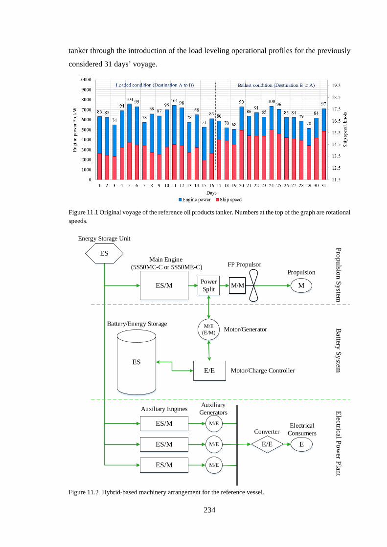
234
tanker through the introduction of the load leveling operational profiles for the previously
considered 31 days’ voyage.
Figure 11.1 Original voyage of the reference oil products tanker. Numbers at the top of the graph are rotational speeds.
Energy Storage Unit
Main Engine (5S50MC-C or 5S50ME-C)
Auxiliary Engines
FP PropulsorPropulsion
Auxiliary Generators
ConverterElectrical
Consumers
Propulsion SystemElectrical Pow
er Plant
ES
ES/M M/M M
ES/M
ES/M
ES/M
E
M/E
M/E
M/E
E/E
Power Split
Battery System
M/E(E/M) Motor/Generator
E/E Motor/Charge ControllerES
Battery/Energy Storage
Figure 11.2 Hybrid-based machinery arrangement for the reference vessel.

235
From a review of recent literature (Whitelegg & Bucknall 2013; DNV GL 2015), the hybrid
system developed in Figure 11.2 was produced as being one of the simplest systems could
be applied to the modern products tanker. The system includes:
• a power split mechanical device which allows to transfer the power between its
connections,
• a battery or energy storage unit that stores an excess power produced by the engine or
supplies demanded power to the propeller if needed,
• a motor/generator acting as a driver of the energy from/to shaft/battery while converting
the energy from mechanical to electrical state and vice versa.
The system may also be equipped with renewable energy technologies or fuel cells for
production and storage of additional power for the battery support purposes. Such a concept
allows the propulsion from the engine or from the motor individually as well as from both
at the same time. In addition, the propeller can also be disconnected for stand-alone
generator functions.
On-Time Voyage Simulation From the operational perspective, the engine load and fuel consumption depend upon the
following factors: required ship speed, ship displacement and weather. In this chapter, two
load-leveling-based operation approaches are considered.
The first concept involves the engine operation based on the average operational speed for
loaded and ballast conditions aiming to complete the voyage on time (referred as
ON_TIME in this study). Therefore, in order to conduct a hybrid-based voyage simulation,
the constant operational engine load and ship speed should be determined.
In this case, a typical 31 days’ voyage, consisting of 16 days at loaded and 15 days at ballast
operations, is considered. The voyage is based on the original FP propeller connected with
the MAN 5S50ME-C marine diesel engine similar to the previous case studies.
The average ship speed for the loaded part of the voyage accounts for 14 knots while in the
case of ballast the average ship speed is 15.1 knots. The ship speed distributions for both
conditions along with their average lines are demonstrated in Figure 11.3.
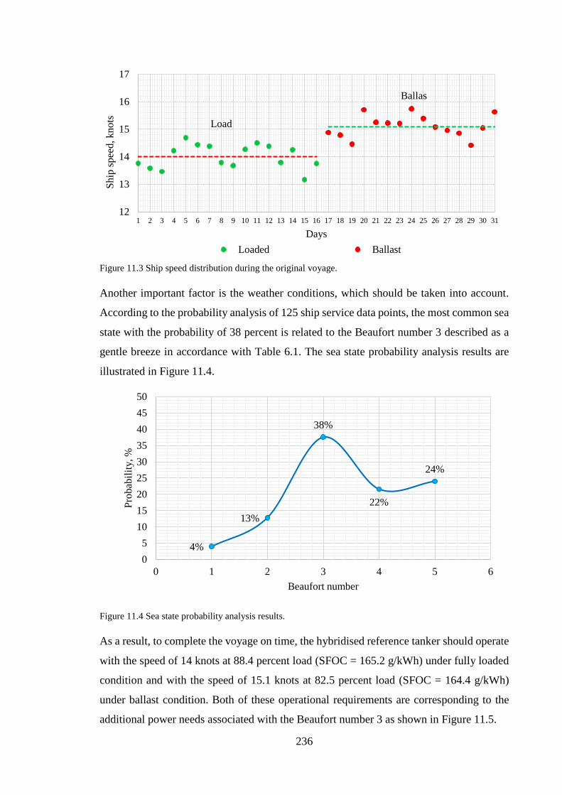
236
Figure 11.3 Ship speed distribution during the original voyage.
Another important factor is the weather conditions, which should be taken into account.
According to the probability analysis of 125 ship service data points, the most common sea
state with the probability of 38 percent is related to the Beaufort number 3 described as a
gentle breeze in accordance with Table 6.1. The sea state probability analysis results are
illustrated in Figure 11.4.
Figure 11.4 Sea state probability analysis results.
As a result, to complete the voyage on time, the hybridised reference tanker should operate
with the speed of 14 knots at 88.4 percent load (SFOC = 165.2 g/kWh) under fully loaded
condition and with the speed of 15.1 knots at 82.5 percent load (SFOC = 164.4 g/kWh)
under ballast condition. Both of these operational requirements are corresponding to the
additional power needs associated with the Beaufort number 3 as shown in Figure 11.5.
12
13
14
15
16
17
1 2 3 4 5 6 7 8 9 10 11 12 13 14 15 16 17 18 19 20 21 22 23 24 25 26 27 28 29 30 31
Ship
spee
d, k
nots
DaysLoaded Ballast
Load
Ballas
4%
13%
38%
22%
24%
05
101520253035404550
0 1 2 3 4 5 6
Prob
abili
ty, %
Beaufort number
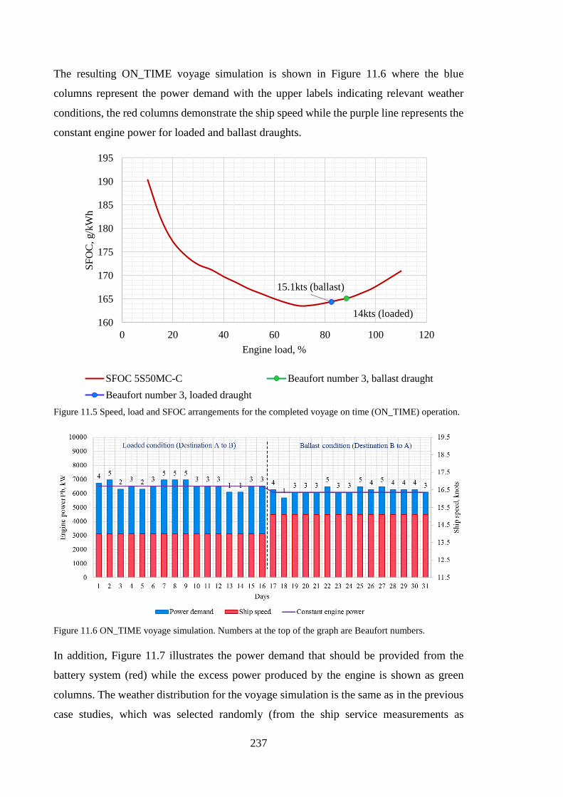
237
The resulting ON_TIME voyage simulation is shown in Figure 11.6 where the blue
columns represent the power demand with the upper labels indicating relevant weather
conditions, the red columns demonstrate the ship speed while the purple line represents the
constant engine power for loaded and ballast draughts.
Figure 11.5 Speed, load and SFOC arrangements for the completed voyage on time (ON_TIME) operation.
Figure 11.6 ON_TIME voyage simulation. Numbers at the top of the graph are Beaufort numbers.
In addition, Figure 11.7 illustrates the power demand that should be provided from the
battery system (red) while the excess power produced by the engine is shown as green
columns. The weather distribution for the voyage simulation is the same as in the previous
case studies, which was selected randomly (from the ship service measurements as
14kts (loaded)
15.1kts (ballast)
160
165
170
175
180
185
190
195
0 20 40 60 80 100 120
SFO
C, g
/kW
h
Engine load, %
SFOC 5S50MC-C Beaufort number 3, ballast draughtBeaufort number 3, loaded draught
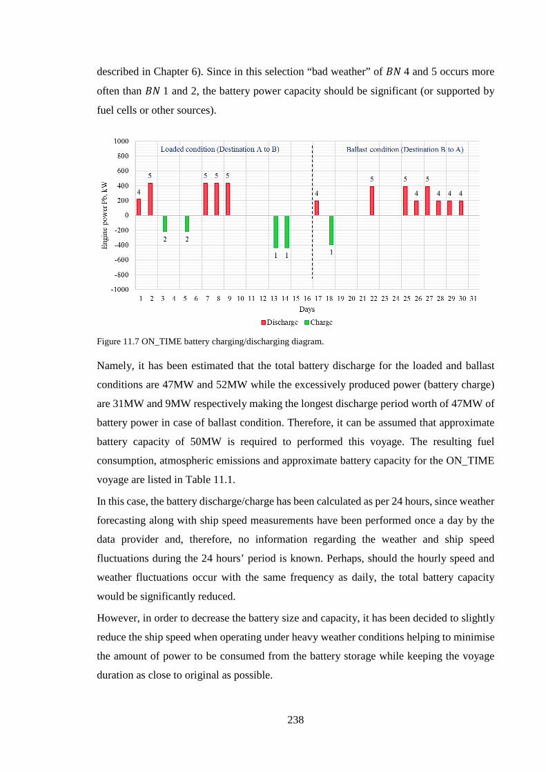
238
described in Chapter 6). Since in this selection “bad weather” of 𝐵𝐵𝑁𝑁 4 and 5 occurs more
often than 𝐵𝐵𝑁𝑁 1 and 2, the battery power capacity should be significant (or supported by
fuel cells or other sources).
Figure 11.7 ON_TIME battery charging/discharging diagram.
Namely, it has been estimated that the total battery discharge for the loaded and ballast
conditions are 47MW and 52MW while the excessively produced power (battery charge)
are 31MW and 9MW respectively making the longest discharge period worth of 47MW of
battery power in case of ballast condition. Therefore, it can be assumed that approximate
battery capacity of 50MW is required to performed this voyage. The resulting fuel
consumption, atmospheric emissions and approximate battery capacity for the ON_TIME
voyage are listed in Table 11.1.
In this case, the battery discharge/charge has been calculated as per 24 hours, since weather
forecasting along with ship speed measurements have been performed once a day by the
data provider and, therefore, no information regarding the weather and ship speed
fluctuations during the 24 hours’ period is known. Perhaps, should the hourly speed and
weather fluctuations occur with the same frequency as daily, the total battery capacity
would be significantly reduced.
However, in order to decrease the battery size and capacity, it has been decided to slightly
reduce the ship speed when operating under heavy weather conditions helping to minimise
the amount of power to be consumed from the battery storage while keeping the voyage
duration as close to original as possible.
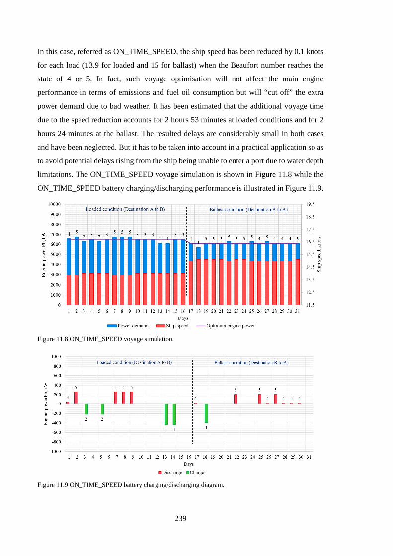
239
In this case, referred as ON_TIME_SPEED, the ship speed has been reduced by 0.1 knots
for each load (13.9 for loaded and 15 for ballast) when the Beaufort number reaches the
state of 4 or 5. In fact, such voyage optimisation will not affect the main engine
performance in terms of emissions and fuel oil consumption but will “cut off” the extra
power demand due to bad weather. It has been estimated that the additional voyage time
due to the speed reduction accounts for 2 hours 53 minutes at loaded conditions and for 2
hours 24 minutes at the ballast. The resulted delays are considerably small in both cases
and have been neglected. But it has to be taken into account in a practical application so as
to avoid potential delays rising from the ship being unable to enter a port due to water depth
limitations. The ON_TIME_SPEED voyage simulation is shown in Figure 11.8 while the
ON_TIME_SPEED battery charging/discharging performance is illustrated in Figure 11.9.
Figure 11.8 ON_TIME_SPEED voyage simulation.
Figure 11.9 ON_TIME_SPEED battery charging/discharging diagram.
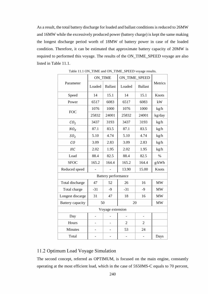
240
As a result, the total battery discharge for loaded and ballast conditions is reduced to 26MW
and 16MW while the excessively produced power (battery charge) is kept the same making
the longest discharge period worth of 18MW of battery power in case of the loaded
condition. Therefore, it can be estimated that approximate battery capacity of 20MW is
required to performed this voyage. The results of the ON_TIME_SPEED voyage are also
listed in Table 11.1.
Table 11.1 ON_TIME and ON_TIME_SPEED voyage results.
Parameter ON_TIME ON_TIME_SPEED
Metrics Loaded Ballast Loaded Ballast
Speed 14 15.1 14 15.1 Knots
Power 6517 6083 6517 6083 kW
FOC 1076 1000 1076 1000 kg/h
25832 24001 25832 24001 kg/day
𝐶𝐶𝐶𝐶2 3437 3193 3437 3193 kg/h
𝑁𝑁𝐶𝐶𝑋𝑋 87.1 83.5 87.1 83.5 kg/h
𝑆𝑆𝐶𝐶2 5.10 4.74 5.10 4.74 kg/h
𝐶𝐶𝐶𝐶 3.09 2.83 3.09 2.83 kg/h
𝐻𝐻𝐶𝐶 2.02 1.95 2.02 1.95 kg/h
Load 88.4 82.5 88.4 82.5 %
SFOC 165.2 164.4 165.2 164.4 g/kWh
Reduced speed - - 13.90 15.00 Knots
Battery performance
Total discharge 47 52 26 16 MW
Total charge -31 -9 -31 -9 MW
Longest discarge 31 47 18 16 MW
Battery capacity 50 20 MW
Voyage extension
Day - - - -
Hours - - 2 2
Minutes - - 53 24
Total - - - - Days
Optimum Load Voyage Simulation The second concept, referred as OPTIMUM, is focused on the main engine, constantly
operating at the most efficient load, which in the case of 5S50MS-C equals to 70 percent,
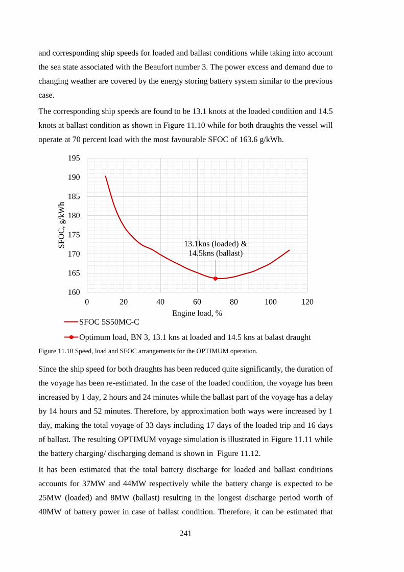
241
and corresponding ship speeds for loaded and ballast conditions while taking into account
the sea state associated with the Beaufort number 3. The power excess and demand due to
changing weather are covered by the energy storing battery system similar to the previous
case.
The corresponding ship speeds are found to be 13.1 knots at the loaded condition and 14.5
knots at ballast condition as shown in Figure 11.10 while for both draughts the vessel will
operate at 70 percent load with the most favourable SFOC of 163.6 g/kWh.
Figure 11.10 Speed, load and SFOC arrangements for the OPTIMUM operation.
Since the ship speed for both draughts has been reduced quite significantly, the duration of
the voyage has been re-estimated. In the case of the loaded condition, the voyage has been
increased by 1 day, 2 hours and 24 minutes while the ballast part of the voyage has a delay
by 14 hours and 52 minutes. Therefore, by approximation both ways were increased by 1
day, making the total voyage of 33 days including 17 days of the loaded trip and 16 days
of ballast. The resulting OPTIMUM voyage simulation is illustrated in Figure 11.11 while
the battery charging/ discharging demand is shown in Figure 11.12.
It has been estimated that the total battery discharge for loaded and ballast conditions
accounts for 37MW and 44MW respectively while the battery charge is expected to be
25MW (loaded) and 8MW (ballast) resulting in the longest discharge period worth of
40MW of battery power in case of ballast condition. Therefore, it can be estimated that
13.1kns (loaded) & 14.5kns (ballast)
160
165
170
175
180
185
190
195
0 20 40 60 80 100 120
SFO
C, g
/kW
h
Engine load, %SFOC 5S50MC-C
Optimum load, BN 3, 13.1 kns at loaded and 14.5 kns at balast draught
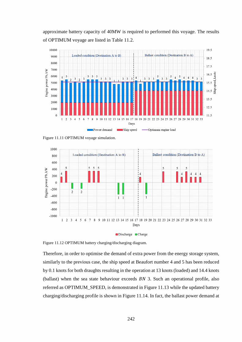
242
approximate battery capacity of 40MW is required to performed this voyage. The results
of OPTIMUM voyage are listed in Table 11.2.
Figure 11.11 OPTIMUM voyage simulation.
Figure 11.12 OPTIMUM battery charging/discharging diagram.
Therefore, in order to optimise the demand of extra power from the energy storage system,
similarly to the previous case, the ship speed at Beaufort number 4 and 5 has been reduced
by 0.1 knots for both draughts resulting in the operation at 13 knots (loaded) and 14.4 knots
(ballast) when the sea state behaviour exceeds 𝐵𝐵𝑁𝑁 3. Such an operational profile, also
referred as OPTIMUM_SPEED, is demonstrated in Figure 11.13 while the updated battery
charging/discharging profile is shown in Figure 11.14. In fact, the ballast power demand at
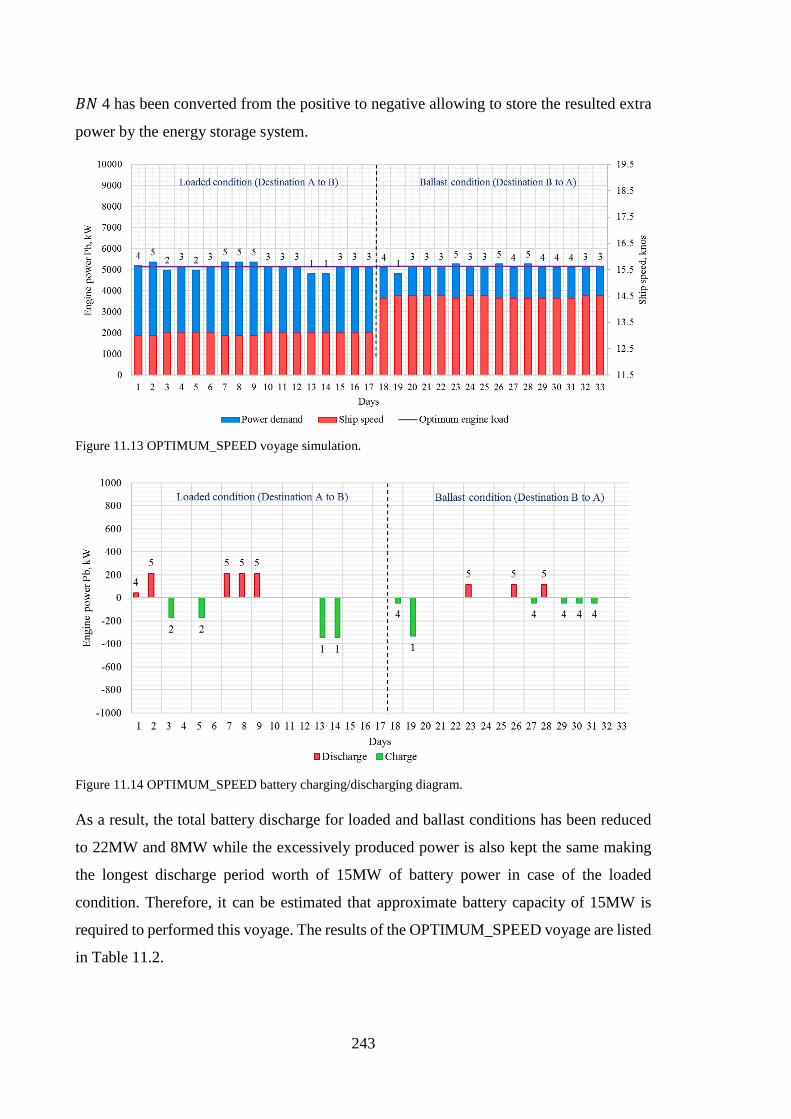
243
𝐵𝐵𝑁𝑁 4 has been converted from the positive to negative allowing to store the resulted extra
power by the energy storage system.
Figure 11.13 OPTIMUM_SPEED voyage simulation.
Figure 11.14 OPTIMUM_SPEED battery charging/discharging diagram.
As a result, the total battery discharge for loaded and ballast conditions has been reduced
to 22MW and 8MW while the excessively produced power is also kept the same making
the longest discharge period worth of 15MW of battery power in case of the loaded
condition. Therefore, it can be estimated that approximate battery capacity of 15MW is
required to performed this voyage. The results of the OPTIMUM_SPEED voyage are listed
in Table 11.2.
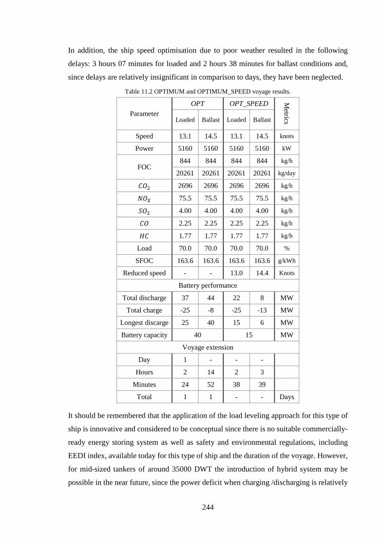
244
In addition, the ship speed optimisation due to poor weather resulted in the following
delays: 3 hours 07 minutes for loaded and 2 hours 38 minutes for ballast conditions and,
since delays are relatively insignificant in comparison to days, they have been neglected.
Table 11.2 OPTIMUM and OPTIMUM_SPEED voyage results.
Parameter OPT OPT_SPEED M
etrics Loaded Ballast Loaded Ballast
Speed 13.1 14.5 13.1 14.5 knots
Power 5160 5160 5160 5160 kW
FOC 844 844 844 844 kg/h
20261 20261 20261 20261 kg/day
𝐶𝐶𝐶𝐶2 2696 2696 2696 2696 kg/h
𝑁𝑁𝐶𝐶𝑋𝑋 75.5 75.5 75.5 75.5 kg/h
𝑆𝑆𝐶𝐶2 4.00 4.00 4.00 4.00 kg/h
𝐶𝐶𝐶𝐶 2.25 2.25 2.25 2.25 kg/h
𝐻𝐻𝐶𝐶 1.77 1.77 1.77 1.77 kg/h
Load 70.0 70.0 70.0 70.0 %
SFOC 163.6 163.6 163.6 163.6 g/kWh
Reduced speed - - 13.0 14.4 Knots
Battery performance
Total discharge 37 44 22 8 MW
Total charge -25 -8 -25 -13 MW
Longest discarge 25 40 15 6 MW
Battery capacity 40 15 MW
Voyage extension
Day 1 - - -
Hours 2 14 2 3
Minutes 24 52 38 39
Total 1 1 - - Days
It should be remembered that the application of the load leveling approach for this type of
ship is innovative and considered to be conceptual since there is no suitable commercially-
ready energy storing system as well as safety and environmental regulations, including
EEDI index, available today for this type of ship and the duration of the voyage. However,
for mid-sized tankers of around 35000 DWT the introduction of hybrid system may be
possible in the near future, since the power deficit when charging /discharging is relatively
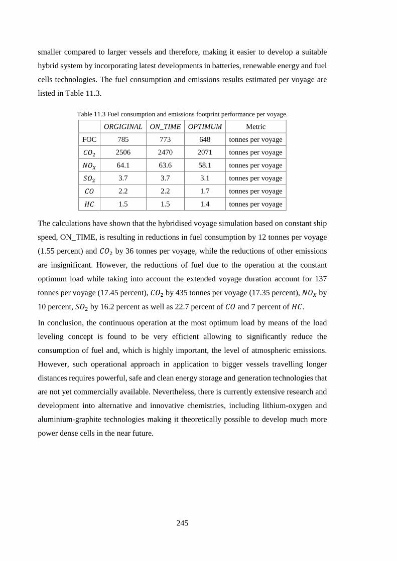
245
smaller compared to larger vessels and therefore, making it easier to develop a suitable
hybrid system by incorporating latest developments in batteries, renewable energy and fuel
cells technologies. The fuel consumption and emissions results estimated per voyage are
listed in Table 11.3.
Table 11.3 Fuel consumption and emissions footprint performance per voyage.
ORGIGINAL ON_TIME OPTIMUM Metric
FOC 785 773 648 tonnes per voyage
𝐶𝐶𝐶𝐶2 2506 2470 2071 tonnes per voyage
𝑁𝑁𝐶𝐶𝑋𝑋 64.1 63.6 58.1 tonnes per voyage
𝑆𝑆𝐶𝐶2 3.7 3.7 3.1 tonnes per voyage
𝐶𝐶𝐶𝐶 2.2 2.2 1.7 tonnes per voyage
𝐻𝐻𝐶𝐶 1.5 1.5 1.4 tonnes per voyage
The calculations have shown that the hybridised voyage simulation based on constant ship
speed, ON_TIME, is resulting in reductions in fuel consumption by 12 tonnes per voyage
(1.55 percent) and 𝐶𝐶𝐶𝐶2 by 36 tonnes per voyage, while the reductions of other emissions
are insignificant. However, the reductions of fuel due to the operation at the constant
optimum load while taking into account the extended voyage duration account for 137
tonnes per voyage (17.45 percent), 𝐶𝐶𝐶𝐶2 by 435 tonnes per voyage (17.35 percent), 𝑁𝑁𝐶𝐶𝑋𝑋 by
10 percent, 𝑆𝑆𝐶𝐶2 by 16.2 percent as well as 22.7 percent of 𝐶𝐶𝐶𝐶 and 7 percent of 𝐻𝐻𝐶𝐶.
In conclusion, the continuous operation at the most optimum load by means of the load
leveling concept is found to be very efficient allowing to significantly reduce the
consumption of fuel and, which is highly important, the level of atmospheric emissions.
However, such operational approach in application to bigger vessels travelling longer
distances requires powerful, safe and clean energy storage and generation technologies that
are not yet commercially available. Nevertheless, there is currently extensive research and
development into alternative and innovative chemistries, including lithium-oxygen and
aluminium-graphite technologies making it theoretically possible to develop much more
power dense cells in the near future.
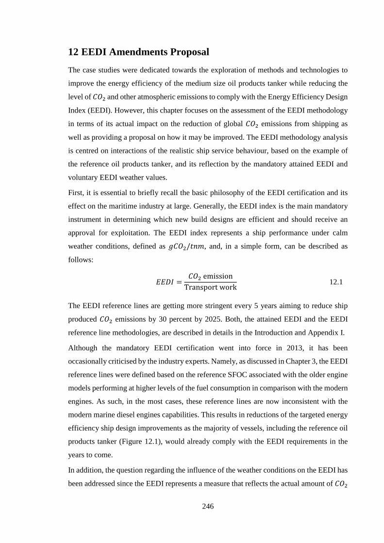
246
12 EEDI Amendments Proposal
The case studies were dedicated towards the exploration of methods and technologies to
improve the energy efficiency of the medium size oil products tanker while reducing the
level of 𝐶𝐶𝐶𝐶2 and other atmospheric emissions to comply with the Energy Efficiency Design
Index (EEDI). However, this chapter focuses on the assessment of the EEDI methodology
in terms of its actual impact on the reduction of global 𝐶𝐶𝐶𝐶2 emissions from shipping as
well as providing a proposal on how it may be improved. The EEDI methodology analysis
is centred on interactions of the realistic ship service behaviour, based on the example of
the reference oil products tanker, and its reflection by the mandatory attained EEDI and
voluntary EEDI weather values.
First, it is essential to briefly recall the basic philosophy of the EEDI certification and its
effect on the maritime industry at large. Generally, the EEDI index is the main mandatory
instrument in determining which new build designs are efficient and should receive an
approval for exploitation. The EEDI index represents a ship performance under calm
weather conditions, defined as 𝑔𝑔𝐶𝐶𝐶𝐶2/𝐶𝐶𝑛𝑛𝑛𝑛, and, in a simple form, can be described as
follows:
𝐸𝐸𝐸𝐸𝐷𝐷𝐸𝐸 =𝐶𝐶𝐶𝐶2 emission
Transport work 12.1
The EEDI reference lines are getting more stringent every 5 years aiming to reduce ship
produced 𝐶𝐶𝐶𝐶2 emissions by 30 percent by 2025. Both, the attained EEDI and the EEDI
reference line methodologies, are described in details in the Introduction and Appendix I.
Although the mandatory EEDI certification went into force in 2013, it has been
occasionally criticised by the industry experts. Namely, as discussed in Chapter 3, the EEDI
reference lines were defined based on the reference SFOC associated with the older engine
models performing at higher levels of the fuel consumption in comparison with the modern
engines. As such, in the most cases, these reference lines are now inconsistent with the
modern marine diesel engines capabilities. This results in reductions of the targeted energy
efficiency ship design improvements as the majority of vessels, including the reference oil
products tanker (Figure 12.1), would already comply with the EEDI requirements in the
years to come.
In addition, the question regarding the influence of the weather conditions on the EEDI has
been addressed since the EEDI represents a measure that reflects the actual amount of 𝐶𝐶𝐶𝐶2
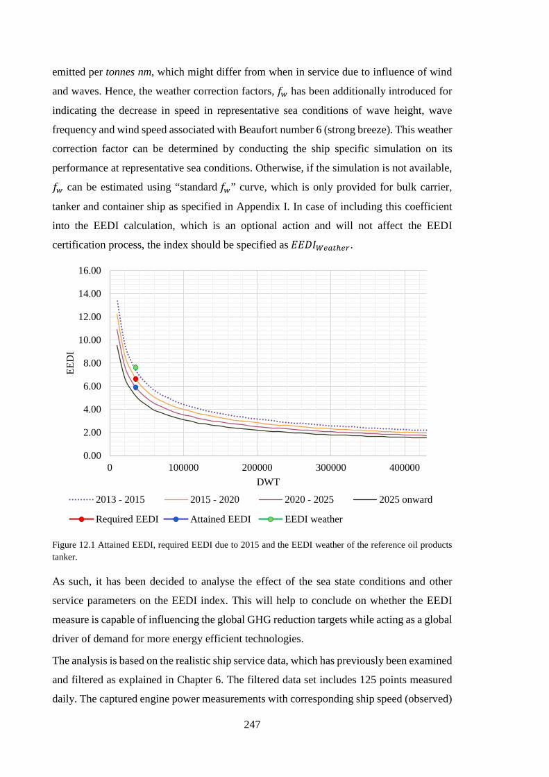
247
emitted per tonnes nm, which might differ from when in service due to influence of wind
and waves. Hence, the weather correction factors, 𝑓𝑓𝑤𝑤 has been additionally introduced for
indicating the decrease in speed in representative sea conditions of wave height, wave
frequency and wind speed associated with Beaufort number 6 (strong breeze). This weather
correction factor can be determined by conducting the ship specific simulation on its
performance at representative sea conditions. Otherwise, if the simulation is not available,
𝑓𝑓𝑤𝑤 can be estimated using “standard 𝑓𝑓𝑤𝑤” curve, which is only provided for bulk carrier,
tanker and container ship as specified in Appendix I. In case of including this coefficient
into the EEDI calculation, which is an optional action and will not affect the EEDI
certification process, the index should be specified as 𝐸𝐸𝐸𝐸𝐷𝐷𝐸𝐸𝑊𝑊𝐴𝐴𝑔𝑔𝐴𝐴ℎ𝐴𝐴𝑟𝑟.
Figure 12.1 Attained EEDI, required EEDI due to 2015 and the EEDI weather of the reference oil products tanker.
As such, it has been decided to analyse the effect of the sea state conditions and other
service parameters on the EEDI index. This will help to conclude on whether the EEDI
measure is capable of influencing the global GHG reduction targets while acting as a global
driver of demand for more energy efficient technologies.
The analysis is based on the realistic ship service data, which has previously been examined
and filtered as explained in Chapter 6. The filtered data set includes 125 points measured
daily. The captured engine power measurements with corresponding ship speed (observed)
0.00
2.00
4.00
6.00
8.00
10.00
12.00
14.00
16.00
0 100000 200000 300000 400000
EED
I
DWT
2013 - 2015 2015 - 2020 2020 - 2025 2025 onward
Required EEDI Attained EEDI EEDI weather
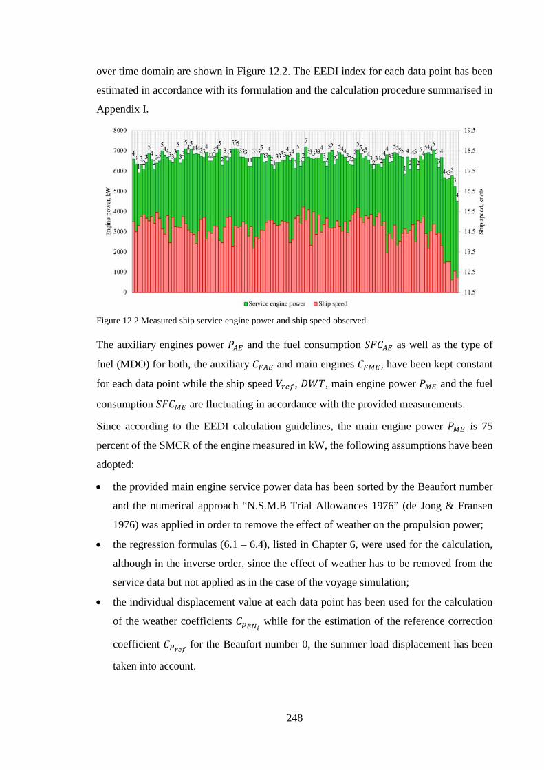
248
over time domain are shown in Figure 12.2. The EEDI index for each data point has been
estimated in accordance with its formulation and the calculation procedure summarised in
Appendix I.
Figure 12.2 Measured ship service engine power and ship speed observed.
The auxiliary engines power 𝑃𝑃𝐴𝐴𝐸𝐸 and the fuel consumption 𝑆𝑆𝑆𝑆𝐶𝐶𝐴𝐴𝐸𝐸 as well as the type of
fuel (MDO) for both, the auxiliary 𝐶𝐶𝐹𝐹𝐴𝐴𝐸𝐸 and main engines 𝐶𝐶𝐹𝐹𝑀𝑀𝐸𝐸 , have been kept constant
for each data point while the ship speed 𝑁𝑁𝑟𝑟𝐴𝐴𝑟𝑟, 𝐷𝐷𝑊𝑊𝑃𝑃, main engine power 𝑃𝑃𝑀𝑀𝐸𝐸 and the fuel
consumption 𝑆𝑆𝑆𝑆𝐶𝐶𝑀𝑀𝐸𝐸 are fluctuating in accordance with the provided measurements.
Since according to the EEDI calculation guidelines, the main engine power 𝑃𝑃𝑀𝑀𝐸𝐸 is 75
percent of the SMCR of the engine measured in kW, the following assumptions have been
adopted:
• the provided main engine service power data has been sorted by the Beaufort number
and the numerical approach “N.S.M.B Trial Allowances 1976” (de Jong & Fransen
1976) was applied in order to remove the effect of weather on the propulsion power;
• the regression formulas (6.1 – 6.4), listed in Chapter 6, were used for the calculation,
although in the inverse order, since the effect of weather has to be removed from the
service data but not applied as in the case of the voyage simulation;
• the individual displacement value at each data point has been used for the calculation
of the weather coefficients 𝐶𝐶𝑖𝑖𝐵𝐵𝑁𝑁𝑖𝑖 while for the estimation of the reference correction
coefficient 𝐶𝐶𝑃𝑃𝑟𝑟𝑟𝑟𝑟𝑟 for the Beaufort number 0, the summer load displacement has been
taken into account.
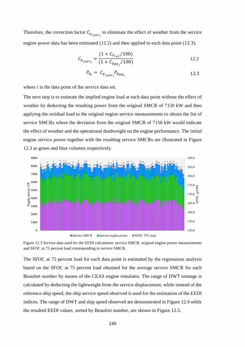
249
Therefore, the correction factor 𝐶𝐶𝑖𝑖𝑐𝑐𝑏𝑏𝑟𝑟𝑟𝑟𝑖𝑖 to eliminate the effect of weather from the service
engine power data has been estimated (12.2) and then applied to each data point (12.3).
𝐶𝐶𝑖𝑖𝑐𝑐𝑏𝑏𝑟𝑟𝑟𝑟𝑖𝑖 =(1 + 𝐶𝐶𝑃𝑃𝑟𝑟𝑟𝑟𝑟𝑟 100⁄ )(1 + 𝐶𝐶𝑖𝑖𝐵𝐵𝑁𝑁𝑖𝑖 100⁄ )
12.2
𝑃𝑃𝐵𝐵𝑖𝑖 = 𝐶𝐶𝑖𝑖𝑐𝑐𝑏𝑏𝑟𝑟𝑟𝑟𝑖𝑖𝑃𝑃𝐵𝐵𝐵𝐵𝑁𝑁𝑖𝑖 12.3
where 𝑖𝑖 is the data point of the service data set.
The next step is to estimate the implied engine load at each data point without the effect of
weather by deducting the resulting power from the original SMCR of 7150 kW and then
applying the residual load to the original engine service measurements to obtain the list of
service SMCRs where the deviation from the original SMCR of 7150 kW would indicate
the effect of weather and the operational deadweight on the engine performance. The initial
engine service power together with the resulting service SMCRs are illustrated in Figure
12.3 as green and blue columns respectively.
Figure 12.3 Service data used for the EEDI calculation: service SMCR, original engine power measurements and SFOC at 75 percent load corresponding to service SMCR.
The SFOC at 75 percent load for each data point is estimated by the regressions analysis
based on the SFOC at 75 percent load obtained for the average service SMCR for each
Beaufort number by means of the CEAS engine simulator. The range of DWT tonnage is
calculated by deducting the lightweight from the service displacement, while instead of the
reference ship speed, the ship service speed observed is used for the estimation of the EEDI
indices. The range of DWT and ship speed observed are demonstrated in Figure 12.4 while
the resulted EEDI values, sorted by Beaufort number, are shown in Figure 12.5.
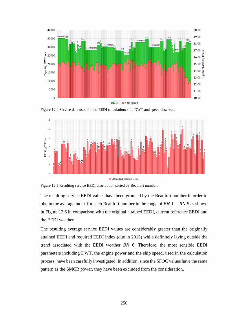
250
Figure 12.4 Service data used for the EEDI calculation: ship DWT and speed observed.
Figure 12.5 Resulting service EEDI distribution sorted by Beaufort number.
The resulting service EEDI values have been grouped by the Beaufort number in order to
obtain the average index for each Beaufort number in the range of 𝐵𝐵𝑁𝑁 1 – 𝐵𝐵𝑁𝑁 5 as shown
in Figure 12.6 in comparison with the original attained EEDI, current reference EEDI and
the EEDI weather.
The resulting average service EEDI values are considerably greater than the originally
attained EEDI and required EEDI index (due in 2015) while definitely laying outside the
trend associated with the EEDI weather 𝐵𝐵𝑁𝑁 6. Therefore, the most sensible EEDI
parameters including DWT, the engine power and the ship speed, used in the calculation
process, have been carefully investigated. In addition, since the SFOC values have the same
pattern as the SMCR power, they have been excluded from the consideration.
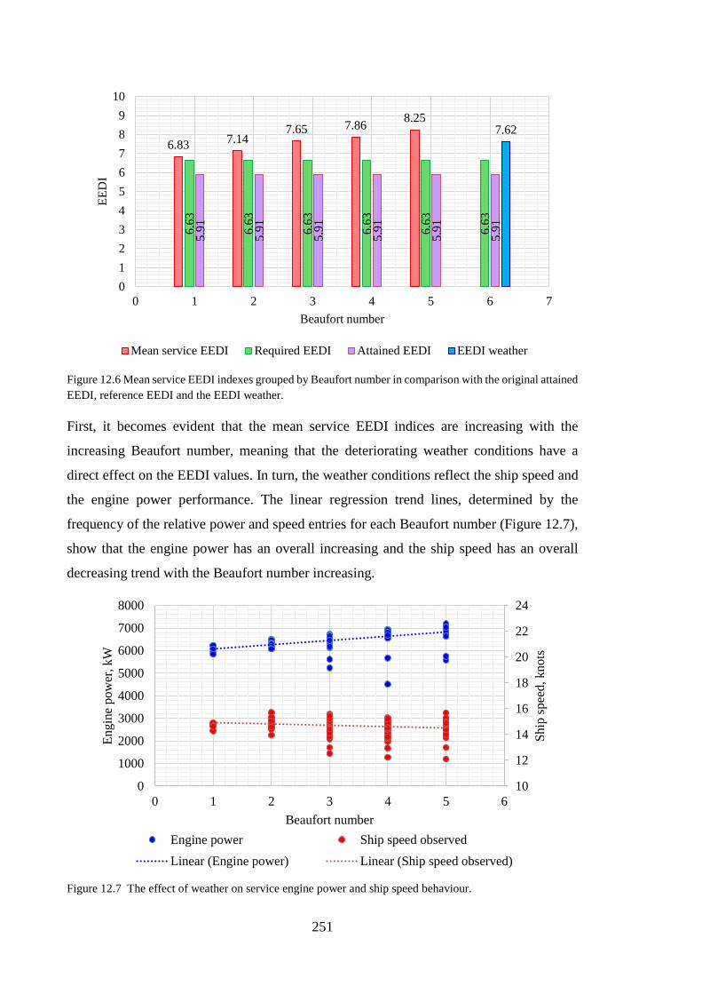
251
Figure 12.6 Mean service EEDI indexes grouped by Beaufort number in comparison with the original attained EEDI, reference EEDI and the EEDI weather.
First, it becomes evident that the mean service EEDI indices are increasing with the
increasing Beaufort number, meaning that the deteriorating weather conditions have a
direct effect on the EEDI values. In turn, the weather conditions reflect the ship speed and
the engine power performance. The linear regression trend lines, determined by the
frequency of the relative power and speed entries for each Beaufort number (Figure 12.7),
show that the engine power has an overall increasing and the ship speed has an overall
decreasing trend with the Beaufort number increasing.
Figure 12.7 The effect of weather on service engine power and ship speed behaviour.
6.83 7.147.65 7.86 8.25
6.63
6.63
6.63
6.63
6.63
6.63
5.91
5.91
5.91
5.91
5.91
5.91
7.62
0123456789
10
0 1 2 3 4 5 6 7
EED
I
Beaufort number
Mean service EEDI Required EEDI Attained EEDI EEDI weather
10
12
14
16
18
20
22
24
0
1000
2000
3000
4000
5000
6000
7000
8000
0 1 2 3 4 5 6
Ship
spee
d, k
nots
Engi
ne p
ower
, kW
Beaufort numberEngine power Ship speed observedLinear (Engine power) Linear (Ship speed observed)
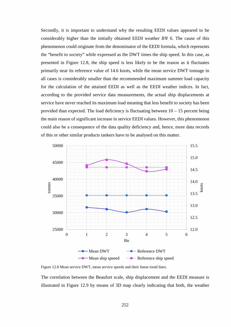
252
Secondly, it is important to understand why the resulting EEDI values appeared to be
considerably higher than the initially obtained EEDI weather 𝐵𝐵𝑁𝑁 6. The cause of this
phenomenon could originate from the denominator of the EEDI formula, which represents
the “benefit to society” while expressed as the DWT times the ship speed. In this case, as
presented in Figure 12.8, the ship speed is less likely to be the reason as it fluctuates
primarily near its reference value of 14.6 knots, while the mean service DWT tonnage in
all cases is considerably smaller than the recommended maximum summer load capacity
for the calculation of the attained EEDI as well as the EEDI weather indices. In fact,
according to the provided service data measurements, the actual ship displacements at
service have never reached its maximum load meaning that less benefit to society has been
provided than expected. The load deficiency is fluctuating between 10 – 15 percent being
the main reason of significant increase in service EEDI values. However, this phenomenon
could also be a consequence of the data quality deficiency and, hence, more data records
of this or other similar products tankers have to be analysed on this matter.
Figure 12.8 Mean service DWT, mean service speeds and their linear trend lines.
The correlation between the Beaufort scale, ship displacement and the EEDI measure is
illustrated in Figure 12.9 by means of 3D map clearly indicating that both, the weather
12.0
12.5
13.0
13.5
14.0
14.5
15.0
15.5
25000
30000
35000
40000
45000
50000
0 1 2 3 4 5 6
knot
s
tonn
es
Bn
Mean DWT Reference DWTMean ship speeed Reference ship speed
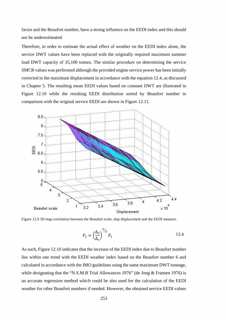
253
factor and the Beaufort number, have a strong influence on the EEDI index and this should
not be underestimated.
Therefore, in order to estimate the actual effect of weather on the EEDI index alone, the
service DWT values have been replaced with the originally required maximum summer
load DWT capacity of 35,100 tonnes. The similar procedure on determining the service
SMCR values was performed although the provided engine service power has been initially
corrected to the maximum displacement in accordance with the equation 12.4, as discussed
in Chapter 5. The resulting mean EEDI values based on constant DWT are illustrated in
Figure 12.10 while the resulting EEDI distribution sorted by Beaufort number in
comparison with the original service EEDI are shown in Figure 12.11.
Figure 12.9 3D map correlation between the Beaufort scale, ship displacement and the EEDI measure.
𝑃𝑃2 = ∆2∆123
𝑃𝑃1 12.4
As such, Figure 12.10 indicates that the increase of the EEDI index due to Beaufort number
lies within one trend with the EEDI weather index based on the Beaufort number 6 and
calculated in accordance with the IMO guidelines using the same maximum DWT tonnage,
while designating that the “N.S.M.B Trial Allowances 1976” (de Jong & Fransen 1976) is
an accurate regression method which could be also used for the calculation of the EEDI
weather for other Beaufort numbers if needed. However, the obtained service EEDI values
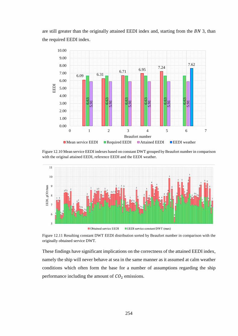
254
are still greater than the originally attained EEDI index and, starting from the 𝐵𝐵𝑁𝑁 3, than
the required EEDI index.
Figure 12.10 Mean service EEDI indexes based on constant DWT grouped by Beaufort number in comparison with the original attained EEDI, reference EEDI and the EEDI weather.
Figure 12.11 Resulting constant DWT EEDI distribution sorted by Beaufort number in comparison with the originally obtained service DWT.
These findings have significant implications on the correctness of the attained EEDI index,
namely the ship will never behave at sea in the same manner as it assumed at calm weather
conditions which often form the base for a number of assumptions regarding the ship
performance including the amount of 𝐶𝐶𝐶𝐶2 emissions.
6.09 6.316.71 6.95 7.24
6.63
6.63
6.63
6.63
6.63
6.63
5.91
5.91
5.91
5.91
5.91
5.91
7.62
0.00
1.00
2.00
3.00
4.00
5.00
6.00
7.00
8.00
9.00
10.00
0 1 2 3 4 5 6 7
EED
I
Beaufort numberMean service EEDI Required EEDI Attained EEDI EEDI weather
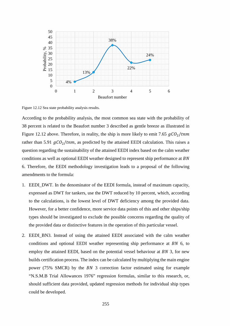
255
Figure 12.12 Sea state probability analysis results.
According to the probability analysis, the most common sea state with the probability of
38 percent is related to the Beaufort number 3 described as gentle breeze as illustrated in
Figure 12.12 above. Therefore, in reality, the ship is more likely to emit 7.65 𝑔𝑔𝐶𝐶𝐶𝐶2/𝐶𝐶𝑛𝑛𝑛𝑛
rather than 5.91 𝑔𝑔𝐶𝐶𝐶𝐶2/𝐶𝐶𝑛𝑛𝑛𝑛, as predicted by the attained EEDI calculation. This raises a
question regarding the sustainability of the attained EEDI index based on the calm weather
conditions as well as optional EEDI weather designed to represent ship performance at 𝐵𝐵𝑁𝑁
6. Therefore, the EEDI methodology investigation leads to a proposal of the following
amendments to the formula:
1. EEDI_DWT. In the denominator of the EEDI formula, instead of maximum capacity,
expressed as DWT for tankers, use the DWT reduced by 10 percent, which, according
to the calculations, is the lowest level of DWT deficiency among the provided data.
However, for a better confidence, more service data points of this and other ships/ship
types should be investigated to exclude the possible concerns regarding the quality of
the provided data or distinctive features in the operation of this particular vessel.
2. EEDI_BN3. Instead of using the attained EEDI associated with the calm weather
conditions and optional EEDI weather representing ship performance at 𝐵𝐵𝑁𝑁 6, to
employ the attained EEDI, based on the potential vessel behaviour at 𝐵𝐵𝑁𝑁 3, for new
builds certification process. The index can be calculated by multiplying the main engine
power (75% SMCR) by the 𝐵𝐵𝑁𝑁 3 correction factor estimated using for example
“N.S.M.B Trial Allowances 1976” regression formulas, similar to this research, or,
should sufficient data provided, updated regression methods for individual ship types
could be developed.
4%
13%
38%
22%
24%
05
101520253035404550
0 1 2 3 4 5 6
Prob
abili
ty, %
Beaufort number
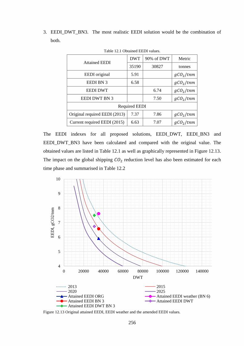
256
3. EEDI_DWT_BN3. The most realistic EEDI solution would be the combination of
both.
Table 12.1 Obtained EEDI values.
Attained EEDI DWT 90% of DWT Metric
35190 30827 tonnes
EEDI original 5.91 𝑔𝑔𝐶𝐶𝐶𝐶2/𝐶𝐶𝑛𝑛𝑛𝑛
EEDI BN 3 6.58 𝑔𝑔𝐶𝐶𝐶𝐶2/𝐶𝐶𝑛𝑛𝑛𝑛
EEDI DWT 6.74 𝑔𝑔𝐶𝐶𝐶𝐶2/𝐶𝐶𝑛𝑛𝑛𝑛
EEDI DWT BN 3 7.50 𝑔𝑔𝐶𝐶𝐶𝐶2/𝐶𝐶𝑛𝑛𝑛𝑛
Required EEDI
Original required EEDI (2013) 7.37 7.86 𝑔𝑔𝐶𝐶𝐶𝐶2/𝐶𝐶𝑛𝑛𝑛𝑛
Current required EEDI (2015) 6.63 7.07 𝑔𝑔𝐶𝐶𝐶𝐶2/𝐶𝐶𝑛𝑛𝑛𝑛
The EEDI indexes for all proposed solutions, EEDI_DWT, EEDI_BN3 and
EEDI_DWT_BN3 have been calculated and compared with the original value. The
obtained values are listed in Table 12.1 as well as graphically represented in Figure 12.13.
The impact on the global shipping 𝐶𝐶𝐶𝐶2 reduction level has also been estimated for each
time phase and summarised in Table 12.2
Figure 12.13 Original attained EEDI, EEDI weather and the amended EEDI values.
4
5
6
7
8
9
10
0 20000 40000 60000 80000 100000 120000 140000
EED
I, gC
O2/
tnm
DWT
2013 20152020 2025Attained EEDI ORG Attained EEDI weather (BN 6)Attained EEDI BN 3 Attained EEDI DWTAttained EEDI DWT BN 3

257
Table 12.2 Impact of amended EEDI values on global 𝐶𝐶𝐶𝐶2 reduction level. Ph
ases
Planned reduction relative to
original baseline
Reduction due to Attained EEDI
ORG
Reduction due to Attained EEDI
BN 3
Reduction due to Attained EEDI DWT
Reduction due to Attained EEDI
DWT BN 3
2013 0% -19.81% -10.67% -14.23% -4.5%
2015 10% -9.81% -0.67% -4.23% 5.5%
2020 20% 0.19% 9.33% 5.77% 15.5%
2025 30% 10.19% 19.33% 15.77% 25.5%
It has been found that the attained EEDI index estimated by means of the conventional
procedure, in case of the reference tanker design, will only lead to 10 percent of 𝐶𝐶𝐶𝐶2
reduction by 2025 instead of targeted 30 percent, while the application of the attained
EEDI_DWT_BN3, which reflects the realistic ship behaviour at sea, will contribute to
some 26 percent of the 𝐶𝐶𝐶𝐶2 reduction level from shipping, which complies with the original
target.
258
13 Conclusion
The primary objective of this PhD project was to develop an advanced understanding of
necessary and realistic performance expectations from full form medium size ship system
by means of numerical computer modelling, in order to minimise the harmful
environmental signature by increasing its efficiency in compliance with the EEDI
requirements while in search of how the EEDI methodology might be enhanced.
To solve such extensive problem, in the first place, the energy efficient technology market
has been analysed in a structured manner while selecting the most favourable fuel
consumption reduction methods applicable to the examined ship type.
Next, an integrated computer Ship Performance Simulation model, involving linked
engine, propeller and hull analysis programs, has been developed and calibrated with the
model tests and sea trial data.
By means of the Ship Performance Simulation model, several case studies have been
conducted where the ship system has been analysed under diverse conditions including
CLT and ducted propulsion systems, energy efficiency-enhancing wake equalising duct
(WED), maximised and optimised propeller designs and trim conditions as well as
innovative hybridised machinery arrangements while taking into account changing weather
and load conditions.
The evaluation of potential benefits associated with the deployment of innovative
technologies, operation profiles and their combination was made by comparing designated
Energy Efficiency Indicators (EEI), namely, the propulsive efficiency, fuel oil
consumption, exhaust emissions footprint and EEDI, respectively associated with the
technical, fuel savings, environmental and legal perspectives.
Energy efficient propellers
The first case study was dedicated to the comparative analysis of four different types of
propulsion systems aiming to explore their effect on the overall ship efficiency performance
by means of holistic ship performance simulation as well as to find the best propeller match
for the medium size tanker/bulk carrier ship types.
• The comparative analysis of fixed pitch propeller with the wake equalizing duct vs. the
conventional fixed pitch propeller has shown an interesting trend of the wake equalizing
duct being the most beneficial at higher ship speeds. In addition, according to the
simulation results, the wake equalizing duct has the most beneficial impact under the
259
loaded conditions rather than ballast while at the ship design speed the maximum
increase of the propulsive efficiency due to the effect of the wake equalizing duct is
found 4.5 percent at the fully loaded (scantling) condition.
• The average reductions of the delivered power by approximately 10 percent have been
found due to the application of the CLT propeller with the wake equalizing duct over
the fixed pitch propeller with the wake equalizing duct system. However, further
fundamental research is needed to ensure that the scaling procedures for this type of
propeller are realistic.
• The power absorption performance of the ducted propeller at different operational
conditions are found to be beneficial in comparison with the conventional fixed pitch
propeller while the ducted propeller performance at ballast condition was slightly better
than at design and loaded conditions. As a result, the maximum power reductions due
to ducted propeller account for approximately 5 percent.
• As a result of the comparative evaluation of the propellers performances between each
other, the most beneficial propeller system is found to be a combination of the open
CLT with the wake equalizing duct (subject to the reservation expressed above),
followed by the open fixed pitch propeller with the wake equalizing duct and the ducted
propeller, although the ducted propeller has shown 3.3 percent better performance at
ballast condition than the conventional fixed pitch with the wake equalizing duct.
• From the fuel economy point of view, the lowest consumption is expected to be
achieved by the CLT propeller performance. However, since a general rate of the
specific fuel oil consumption of 5S46ME-B engine is slightly higher than that of
5S50ME-C engine, the SFOC of the CLT propeller at NCR is by 1.4 percent exceeding
the conventional fixed pitch propeller, while the lowest SFOC rate of 164.3 g/kWh is
achieved by the fixed pitch propulsion system with the wake equalizing duct.
• Regarding the exhaust emissions footprint, it is possible, again taking into account the
above reservation, to reduce the 𝐶𝐶𝐶𝐶2 emissions by 14.7 percent by adopting the CLT
propeller and by about 5 percent by applying the wake equalizing duct or ducted
propeller. It is also possible to reduce 𝑁𝑁𝐶𝐶𝑋𝑋 emissions by 17.3 percent with the CLT
propeller and by approximately 4.8 percent with the ducted propeller or the wake
equalizing duct.
• In terms of the EEDI index, the application of wake equalizing duct and ducted
propellers for such ship types and design will satisfy the EEDI requirements up to 2020,

260
while the reference ship design arrangements with the application of the CLT propeller
will almost meet the 2025 EEDI expectations.
• Since the ducted propeller is more beneficial at ballast condition, its voyage
performance is found to be more advantageous vs. fixed pitch propeller with the wake
equalizing duct achieving the possible savings of 4 tonnes of fuel per voyage, while the
CLT propeller application resulted in savings of 93 tonnes of fuel per voyage compared
to the conventional FPP.
Propeller optimisation
Two propeller optimisation techniques, a reduction of the blade area ratio and an artificial
increase of the propeller diameter, have been analysed in this case study.
• In the case of reduction of the blade area ratio to its possible minimum (0.4), the power
absorption is found to be 1.54 percent lower than in the case of the optimum blade area
ratio, however, this would significantly increase a chance of development of the back
cavitation on the propeller blades. Nevertheless, with growing R&D interests in
developing of the anti-cavitation materials and coating, a chance to incorporate more
hydrodynamically efficient propellers with reduced blade area ratio without the fear of
cavitation will significantly increase.
• In turn, the artificially increased propeller diameter has also shown a positive influence
onto the overall propulsive efficiency, although slightly lower than in case of the
reduction of the blade area ratio, with achieved reductions in the delivered power
requirements by 1.07 percent when increasing the original propeller diameter by 5
percent (D = 5.93m).
• The increase of the propeller diameter (with decreasing blade area ratio) will not affect
the cavitation performance since the excessive thrust loading would be evenly
distributed along a larger surface of the propeller disc. However, even 5 percent
increase of the optimum diameter will give a rise to the hull surface pressure pulses,
resulting in a potential intensification of the inboard noise and vibration. In addition,
the increase of the propeller diameter results in a decrease in the average wake fraction,
resulting in the overall decrease in the hull efficiency.
The Energy Efficiency Indicators analysis has shown that the application of such propeller
systems alone will not significantly affect the emissions footprint and the EEDI index,
however, they will provide some fuel savings while might be a useful bonus when
combined with other energy saving devices.

261
• The lowest fuel consumption, as expected, is achieved by the propeller with reduced
blade area ratio, which is on 19 kg/h lower than the conventional fixed pitch propeller
requirements.
• Regarding the exhaust emissions footprint, it is possible to reduce the 𝐶𝐶𝐶𝐶2 emissions
by 1.8 percent by adopting the propeller with reduced blade area ratio and by about 1
percent by artificially increasing the propeller diameter by 5 percent. However, almost
no changes were found in case of 𝑁𝑁𝐶𝐶𝑋𝑋 emissions footprint in both cases.
• The scale of EEDI fluctuations due to the propeller optimisation for both cases is small
and does not have any significant impact on the EEDI certification process.
• In addition, the possible savings of 6 tonnes of fuel per voyage could be achieved by
increasing the propeller diameter by 5 percent, while the installation of the fixed pitch
propeller with reduced blade area ratio would contribute to the fuel reduction of 11
tonnes per voyage.
Maximum propeller diameter
Two low RPM/increased diameter propeller design concepts based on the conventional
fixed pitch propellers, namely the system with the maximum diameter that could be fitted
into the current ship arrangement and the system with the maximum possible diameter
involving the shaft relocation, have been analysed.
• The average reduction due to maximising the propeller diameter while minimising its
rotational speed accounts for 6 percent in the case of maximised propeller with the
initial shaft arrangements and 7.3 percent for the maximised propeller with the lifted
shaft.
• In the case of retrofitting, both systems will require a significant financial effort to
provide new propeller, super slow diesel engine as well as to modify the transmission
system to perform the shaft relocation.
• For new builds, maximising the propeller diameter is a good option to save up to 50
tonnes of fuel per voyage, being especially profitable should the fuel prices increase,
reducing the 𝐶𝐶𝐶𝐶2 emissions by almost 200 kg per hour and 𝑁𝑁𝐶𝐶𝑋𝑋 by 17 kg per hour
while complying with the EEDI index requirements up to 2020. In addition, there is no
need for shaft relocation should the propeller size be confirmed before the power plant
selection, making the preliminary ship performance simulation an important part of the
efficient ship design.
262
Trim optimisation
The case study is performed with the reference to -1.75m and 1m trim conditions
representing a partially loaded draught of 8 m at an even keel. These trims have been
selected in accordance with the waterline fluctuations around the bulbous bow while the
variations around the stern are kept constant.
• It has been found that the forward trim = - 1.75m is the most beneficial option with the
maximum delivered power reductions by 9.2 percent in comparison to the even keel
while the energy losses due to trim = 1m can reach up to 19.4 percent with increasing
speed.
• The engine simulation results have shown that it is possible to reduce fuel oil
consumption by more than 5 percent when operating at trim = -1.75m compare to the
even keel, while if the trim was not properly optimised (trim = 1m), the fuel losses
reach up to 15 percent in contrast with the even keel.
• Regarding the exhaust emissions footprint, it is possible to reduce the 𝐶𝐶𝐶𝐶2 emissions
by 5.3 percent and the 𝑁𝑁𝐶𝐶𝑋𝑋 emissions by 3.6 percent in the case of the optimised trim
(trim = -1.75m), while the 𝐶𝐶𝐶𝐶2 and 𝑁𝑁𝐶𝐶𝑋𝑋 emissions will increase by 15.3 and 9.3 percent
respectively at the poorly optimised trim (trim = 1m).
• The fuel savings with the optimised trim (trim = -1.75m) account for 11 tonnes of fuel
per voyage, while losses due to trim = 1m reach up to 41 tonnes of fuel per voyage.
Therefore, the results have shown that the impact of trim on ship efficiency is significant
and, if not optimised properly, can lead to serious power losses, while minimising the
benefits of energy saving devices and high-efficiency propellers as well as the initial
purpose of the EEDI certification.
On the other end of the spectrum, the trim optimisation is difficult to control
governmentally, since it has to be performed in each individual case depending on load,
speed and the hull structure. However, the industry’s interests in fuel savings and
environmental concerns regarding the exhaust emissions control coupled with the growing
trim optimisation CFD based software development could lead to some additional
improvements addressed to the EEDI legislation, namely to include the trim optimisation
software installation as a mandatory requirement to a ship owner in order to be issued with
the EEDI certificate.
263
Future hybrid propulsion concepts
The case study is dedicated towards the evaluation of the potential benefits and savings due
to hybridisation of the reference tanker trough the introduction of the load leveling
operational profiles for the previously considered 31 days’ voyage.
• As a result, the continuous operation at the most optimum load by means of load
leveling concept is found to be very efficient allowing to significantly reduce the
consumption of fuel and more importantly the level of atmospheric emissions.
• The reductions of fuel due to the operation at the constant optimum load while taking
into account the extended voyage duration account for 137 tonnes per voyage (17.45
percent), 𝐶𝐶𝐶𝐶2 by 435 tonnes per voyage (17.35 percent), 𝑁𝑁𝐶𝐶𝑋𝑋 by 10 percent, 𝑆𝑆𝐶𝐶2 by
16.2 percent as well as 22.7 percent of 𝐶𝐶𝐶𝐶 and 7 percent of 𝐻𝐻𝐶𝐶.
However, such operational approach in the application for bigger vessels travelling longer
distances requires powerful, safe and clean energy storage and generation technologies that
are not yet commercially available. On the positive note, there is currently extensive
research and development into alternative and innovative chemistries, including lithium-
oxygen and aluminium-graphite technologies making it theoretically possible to develop
much more power dense cells in the near future.
EEDI methodology assessment
The EEDI methodology’s ability to act as a global driver for cleaner shipping has been
analysed in this study.
• It has been found that the current EEDI methodology does not fully reflect the realistic
ship performance at sea while the attained EEDI estimated by means of the
conventional procedure, in case of the reference tanker design, will only lead to 10
percent of 𝐶𝐶𝐶𝐶2 reduction by 2025 instead of the targeted 30 percent.
Therefore, it has been proposed to enhance the EEDI methodology be applying the
following corrections:
• In the denominator of the EEDI formula, instead of maximum capacity, expressed as
DWT for tankers, use the DWT reduced by 10 percent, which, according to the
calculations, is the lowest level of DWT deficiency among the provided data. However,
for a better confidence, more service data points of this and other ships/ship types
should be investigated to exclude the possible concerns regarding the quality of the
provided data or distinctive features in the operation of this particular vessel.

264
• Instead of using the attained EEDI associated with the calm weather conditions and
optional EEDI weather representing ship performance at 𝐵𝐵𝑛𝑛 6, to employ the attained
EEDI, based on the potential vessel behaviour at 𝐵𝐵𝑛𝑛 3, for new builds certification
process. The index can be calculated by multiplying the main engine power (75%
SMCR) by the 𝐵𝐵𝑛𝑛 3 correction factor estimated using for example “N.S.M.B Trial
Allowances 1976” regression formulas, as in this research, or, should sufficient data
provided, updated regression methods for individual ship types could be developed.
However, the most realistic EEDI solution would be a combination of both.
• As a result, the application of the consistent with reality attained EEDI with reduced
DWT and associated with the 𝐵𝐵𝑛𝑛 3 will contribute to some 26 percent of the 𝐶𝐶𝐶𝐶2
reduction level from shipping, which almost perfectly complies with the original target.
• In addition, a stipulation to include the on-board trim optimisation software as a
mandatory requirement to a ship owner in order to be issued with the EEDI certificate
will help to ensure that the ship is operating with the same environmental signature as
it is required by the legal authorities.
265
14 Recommendations
Recommendations for the medium size ship system
The medium size ship system may benefit from:
• the installation of a CLT propeller in combination with the wake equalizing duct;
• the maximised propeller diameter with reduced rotational speed for new build
application;
• careful trim optimisation by means of on-board computer simulations will help to
maximise the hull design beneficial features and to save more fuel.
In long term perspective:
• the minimisation of propeller’s blade area ratio (should the cavitation resistant propeller
materials or coatings be introduced to the market);
• the continuous operation at the most optimum load by means of load leveling concept
will bring significant reductions in emissions and fuel consumption as well as stabilised
engine exploitation.
EEDI methodology recommendations
• to employ the attained EEDI, based on the potential vessel behaviour at 𝐵𝐵𝑁𝑁 3 for new
builds certification purposes.
Therefore, in the numerator of the EEDI formula:
• to add the 𝐵𝐵𝑁𝑁 3 correction factor estimated using for example N.S.M.B Trial
Allowances regression formulas, or, should sufficient data be provided, updated
regression methods for individual ship types could be developed.
In the denominator of the EEDI formula:
• instead of maximum capacity, expressed as DWT for tankers, to use the DWT reduced
by 10 percent.
In addition:
• to include on-board trim optimisation software as a mandatory requirement for a
successful EEDI certification.

266
15 Suggestions for Further Research
• To develop a model to full scale method of scaling the CLT propellers;
• to better understand the margins against cavitation erosion for propellers;
• to perform a research into alternative chemistries to create lighter in weight but higher
power-dense battery cells suitable for bigger ship’s main propulsion system;
• to expand the Ship Performance Simulation model to include the assessment and
prediction of ship performance under changing fuel prices and freight rates;
• to expand the Ship Performance Simulation model for other ship types;
• to create an alternative regression method using latest ship performance data for
estimation of the EEDI weather correction factors suitable for a range of ship types and
sizes to reflect a realistic ship performance under representative weather conditions.
267
References
ABS, 2013. Ship energy efficiency measures.
AEA Energy and Environment, 2008. Greenhouse gas emissions from shipping: trends, projections and abatement potential.
Aertssen, G., 1963. Service perfomance and seakeeping trials on MV Lukuga. The Royal Institution of Naval Architects, 105, pp.293–335.
Anderson, J., 2015. Development of hybrid propulsion for small ro-pax ferries and the feasibility of a zero emissions hydrogen fuel cell powered ferry. City University London.
Anderson, M., Salo, K. & Fridell, E., 2015. Particle and gaseous emissions from an LNG powered ship. Environmental Science & Technology, 49(20), pp.12568–12575.
Anink, D. & Krikke, M., 2011. Analysis of the effects of the new EEDI requirements on Dutch build and flagged ships. , pp.1–46.
Bagniewski, M., 2013. LNG fuel for ships. A chance or a must? DNV GL.
Banisoleiman, K. et al., Simulation of diesel engine performance. Trans IMarE, 105(3), pp.117–135.
Bertram, V., 2012. Practical Ship Hydrodynamics, Elsevier.
Boer, E. & Hoen, M., 2015. Scrubbers – an economic and ecological assessment.
BP, 2015. BP statistical review of world energy.
Bregliozzi, G. et al., 2005. Cavitation wear behaviour of austenitic stainless steels with different grain sizes. Wear, 258(1–4), pp.503–510.
Breslin, J.P. & Andersen, P., 1994. Hydrodynamics of ship propellers, Cambridge Ocean Technology Series.
Burrill, L.C., 1943. Developments in propeller design and manufacture for merchant ships. Trans. of the Institute of Marine Engineers.
Carlton, J., 2012. Marine Propellers and Propulsion 3rd ed., Elsevier.
Carlton, J.S., Smart, R. & Jenkins, V., 2011. The nuclear propulsion of merchant ships: aspects of engineering, science and technology. Proceedings of the Institute of Marine Engineering, Science and Technology Part A: Journal of Marine Engineering and Technology, 10(2), pp.47–59.
Çelik, F., 2007. A numerical study for effectiveness of a wake equalizing duct. Ocean Engineering, 34(16), pp.2138–2145.
Chryssakis, C. et al., 2014. Alternative fuels for shipping. , pp.1–28.
Corbett, J.. et al., 2009. Second IMO GHG study.
Corbett, J.J. et al., 2007. Mortality from ship emissions: a global assessment. Environmental science & technology, 41(24), pp.8512–8.
Corbett, J.J. & Winebrake, J., 2008. The impacts of globalisation on international maritime transport activity, Guadalajara, Mexico.

268
Crist, P., 2009. Greenhouse gas emissions reduction potential from international shipping.
Dedes, E. et al., 2011. Possible power train concepts for nuclear powered merchant ships.
DNV GL, 2015. In focus - the future is hybrid: a guide to use batteries in shipping.
Eastop, T.D. & McConkey, A., 1993. Applied thermodynamics for engineering technologists, Wiley.
Egnell, R., 1998. Combustion diagnostics by means of multizone heat release analysis and NO calculation.. Sae.
Faber, J. et al., 2015. Estimated index values of new ships - analysis of EIVs of ships that have entered the fleet since 2009. , (March).
Faber, J., 2015. Historical trends in ship design efficiency. , (March).
Flagan, R.C. & Seinfeld, J.H., 1988. Fundamentals of air pollution engineering, Prentice-Hall, Inc., Englewood Cliffs, New Jersey.
Florentinus, A., 2012. Potential of biofuels for shipping.
Flynn, D., 2003. Thermal power plant simulation and control, Institution of Engineering and Technology.
Freund, R.J. & Wilson, W.J., 2003. Statistical methods B. Holland, ed., Academic Press.
Gazley, I., 2007. UK environmental accounts: air emissions and energy use. Economic #38; Labour Market Review, 1(11), pp.18–27.
Germanischer Lloyd, 2013. Guidelines for determination of the Energy Efficiency Design Index.
Ghose, P.J.P. & Gokarn, R.P., 2009. Basic ship propulsion, Allied Publishers.
Grim, O., 1980. Propeller and vanewheel. Second George Weinblum Memorial Lecture, J. Ship. Res, December(24(4)).
Grothues-Spork, K., 1988. Bilge vortex control devices and their benefits for propulsion. International Shipbuilding Progress, 35(402).
Hansen, H., Gmbh, F. & Germany, P., 2012. Assistance tools for operational fuel efficiency. 9th Conference on Computer and IT Applications, pp.356–366.
Harrould-Kolieb, E., 2008. Shipping impacts on climate: a source with solution. Oceana, (July).
Harvald, S.A., 1983. Resistance and propulsion of ships.
Heywood, J.B., 1985. Internal combustion engine.
Hirdaris, S.E. et al., 2014. Considerations on the potential use of Nuclear Small Modular Reactor (SMR) technology for merchant marine propulsion. Ocean Engineering, 79, pp.101–130.
Hollenbach, K.U., 1998. Estimating resistance and propulsion for single-screw and twin-screw ships. Ship Technology Research, 45(2), pp.72–76.
Holsonback, C. et al., 2006. System-level modelling and optimal design of an all- electric ship energy storage module.
269
Holtrop, J., 1984. A statistical re-analysis of resistance and propulsion data. International shipbuilding progress, 31(363), pp.272–276.
Holtrop, J. & Mennen, J.G.G., 1982. An approximate power prediction method.
Hountalas, D., Sakellaridis, N. & Zovanos, G., 2013. Optimization of 2- stroke marine diesel engine fuel consumption via VIT setting using a model based monitoring & diagnosis technique: on-board test case. In International Council on Combustion Engines.
IMO, 2014a. Resolution MEPC.245(66): 2014 guidelines on the method of calculation of the attained Energy Efficiency Design Index (EEDI) for new ships., 245(April).
IMO, 2013. Resolution MEPC. 231(65): 2013 Guidelines for calculation of reference lines for use with the Energy Efficiency Design Index (EEDI)., 231(May), pp.1–12.
IMO, 2014b. Third IMO GHG study.
IMO MEPC 63/INF.2, I.M.O., Bazari, Z. & Longva, T., 2011. Assessment of IMO mandated energy efficiency measures for international shipping: estimated CO2 emissions reduction from introduction of mandatory
IPCC, 2014. Summary for policymakers in: climate change 2014, mitigation of climate change. Contribution of working group III to the fifth assessment report of the intergovernmental panel on climate change
ITTC, 1999. Final report of the specialist committee on unconventional propulsors., (February).
Jin, W. & Vassalos, D., 2013. Energy modeling of large 2-stroke marine diesel engine using CFD.
de Jong, H.J. & Fransen, H.P., 1976. N.S.M.B. trial allowances 1976., pp.319–320.
Kawabuchi, M. et al., 2011. CFD predictions of bubbly flow around an energy-saving ship with Mitsubishi air lubrication system. Mitsubishi Heavy Industries Technical Review, 48(1), pp.53–57.
Kim, K.-H. & Fraas, J.F., 1992. Propeller parametric study for mid-term fast sealift ships. Proceedings of the Twenty-Third American Towing Tank Conference, pp.195–2001.
Klimt-Møllenbach, C. et al., 2012. ECA retrofit technology.
Koronowicz, T. et al., 2010. A complete design of contra-rotating propellers using the new computer system. Polish Maritime Research, 17(1), pp.14–24.
Kristensen, H.O., 2012. Energy demand and exhaust gas emissions of marine engines.
Lauer, A. et al., 2007. Global model simulations of the impact of ocean-going ships on aerosols, clouds, and the radiation budget. Atmospheric Chemistry and Physics Discussions, 7(4), pp.9419–9464.
Leigh-Jones, C., 2008. A practical guide to marine fuel oil handling, IMarEST.
Lun, Y.H. (Venus), Lai, K.H. & Cheng, T.C.E., 2010. Shipping and logistics management, Springer.
MAN Diesel and Turbo, 2015. Diesel-electric propulsion plants. , pp.1–27.
MAN Diesel and Turbo, Exhaust gas emission comtrol today and tomorrow: application

270
on MAN B&W two-stroke marine diesel engines.
MAN Diesel and Turbo, 2011. G-type engine: revolutionary ultra-long-stroke.
MAN Diesel and Turbo, 2014a. Low container ship speed facilitated by versatile ME/ME-C engines.
MAN Diesel and Turbo, 2014b. Marine engine IMO Tier ll programme 2014.
MAN Diesel and Turbo, 2014c. Thermo efficiency system for reduction of fuel consumption and CO2 emissions.
MAN Diesel and Turbo, 2014d. Waste Heat Recovery System (WHRS) for reduction of fuel consumption, emissions and EEDI.
Mcgill, R., Remley, W. & Winther, K., 2013. Alternative fuels for marine applications. , (May).
MEPC.1/Circ.683, 2009. Guidence for the development of a ship energy efficiency management plan (SEEMP).
MEPC.1/Circ.684, 2009. Guidelines for voluntary use of the ship Energy Efficiency Operational Indicator (EEOI).
MEPC.1/Circ.796, 2012. Interim guidelines for the calculation of the coefficient fw for decrease in ship speed in a representative sea condition for trial use. , 44(0).
MEPC.177(58) Annex 14, 2010. Amendments to the technical code on control of emissions of nitrogen oxides from marine diesel engines. In pp. 1–101.
MEPC.184(59) Annex 9, 2010. 2009 guidelines for exhaust gas cleaning systems. , 184(July), pp.1–24.
MEPC.207(62) Annex 26, 2011. 2011 guidelines for the control and management of ships “bio fouling” to minimize the transfer of invasive aquatic species. , 207(July), pp.1–25.
MEPC.213(63), 2012. 2012 guidelines for the development of a Ship Energy Efficiency Management Plan (SEEMP).
MEPC 12th Session & Agenda Item 6, 2007. Review of Marpol Annex VI and NOx technical code.
MEPC 212(63) Annex 8, 2012. Guidelines on the method of calculation of the attained Energy Efficiency Design Index (EEDI) for new ships.
MEPC 53th Session & Agenda Item 4, 2005. Prevention of air pollution from ships: MARPOL Annex 6.
MEPC 57th Session & Agenda Item 4, 2008. Prevention of air pollution from ships: CO2 emissions index per unit shipping capacity., (January), pp.1–2.
MEPC 58th Session & Agenda Item 4, 2008a. Prevention of air pollution from ships: proposal for refining the draft formula for CO2 design index for new ships., (August), pp.5–8.
MEPC 58th Session & Agenda Item 4, 2008b. Prevention of air pollution from ships: report of the outcome of the first intersessional meeting of the working group on greenhouse gas emissions from ships., (July).

271
MEPC 68/INF.30, 2015. 2015 industry guidelines on calculation and verification of the Energy Efficiency Design Index (EEDI)., 30.
MER, 2012. Driving fuel costs down. Marine Engineers Review, (April).
Metz, B., 2007. Climate change 2007.
Molland, A.F., Turnock, S.R. & Hudson, D.A., 2011. Ship resistance and propulsion, Cambridge University Press.
Mortensen, N.B., 2009. Ship fuel efficiency in a historical perspective. BIMCO Bulletin, 104(1), pp.38–46.
Moulijn, J.C. et al., 2006. A criterion for the erosiveness of face cavitation. In 6th International Symposium on Cavitation CAV2006. Wageningen.
Munro-Smith, R., Ships and naval architecture, Hobbs.
Murphy, J. et al., 2013. Modelling ship emmission factors and emission indicies. Low Carbon Shipping Conference 2013, p.18.
Ok, J.P., 2004. Numerical investigation of scale effects of Schneekluth’s duct. Hamburg Technical University, Germany.
Oosterveld, M.W.C. & Van Oossanen, P., 1975. Further computer-analyzed data of the Wageningen B-screw series. International Shipbuilding Progress, 22(251).
Papanikolaou, A., 2014. Ship design : methodologies of preliminary design, Springer.
Perez Gomez, G. & Gonzalez-Adalid, J., 1998. Detailed design of ship propellers, F.E.I.N.
Pestana, H., 2014. Future trends of electrical propulsion and implications to ship design.
RAE, 2013. Future ship powering options.
Reichel, M., Minchev, A. & Larsen, N.L., 2014. Trim optimisation - theory and practice., 8(3), pp.387–392.
RINA, 1973. RINA simposium on ducted propellers., London.
Schneekluth, H. & Bertram, V., 1998. Ship design for efficiency and economy 2nd, ed. ButterworthHeinemann, p.226.
Siemens, 2013. SINAVY PEM fuel cell.
Smith, T., Argyros, D., et al., 2014. Global marine fuel trends 2030.
Smith, T., Day, S., et al., 2014. Low carbon shipping – a systems approach.
Suarez, S., Fuente, D. & Greig, A.R., 2013. Making shipping greener : ORC modelling in challenging environments. , pp.1–17.
Torvanger, A. et al., 2007. Climate regulation of ships.
Townsend, C., 2009. Marine fuels and engines. Naval Architect, Guido Perla & Associates, Inc.
Townsin, R.L. et al., 1980. Speed, power and roughness: the economics of outer bottom maintenance. Naval Architect, (5), pp.459–483.
Trodden, D. & Woodward, M., 2013. Reduction of greenhouse gas emissions by propeller design for ship-in-service conditions. Powering and performance methodology.
272
Tsimplis, M. et al., 2012. Regulated slow steaming in maritime transport: an assessment of options, costs and benefits.
UNCTAD, 2015. Review of maritime transport.
UNFCCC, 1998. Kyoto protocol to the United Nations framework. Review of European Community and International Environmental Law, 7(2), pp.214–217.
Veenman, H. & Zonen, N. V., 1970. Wake adapted ducted propellers.
Wärtsilä, 2010. Boosting energy efficiency.
Whitelegg, I. & Bucknall, R., 2013. Electrical propulsion in the low carbon economy., pp.1–13.
Woodyard, D., 2009. Pounder’s marine diesel engines and gas turbines 9th ed. D. Woodyard, ed., Elsevier.
Woud, H.K. & Stapersma, D., 2012. Design of propulsion and electric power generation systems,
Yamatogi, T. et al., 2009. Study on cavitation erosion of composite materials for marine propeller. University of Tokyo.
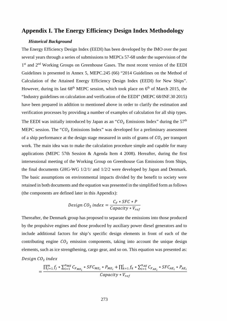
273
Appendix I. The Energy Efficiency Design Index Methodology
Historical Background
The Energy Efficiency Design Index (EEDI) has been developed by the IMO over the past
several years through a series of submissions to MEPCs 57-68 under the supervision of the
1st and 2nd Working Groups on Greenhouse Gases. The most recent version of the EEDI
Guidelines is presented in Annex 5, MEPC.245 (66) “2014 Guidelines on the Method of
Calculation of the Attained Energy Efficiency Design Index (EEDI) for New Ships”.
However, during its last 68th MEPC session, which took place on 6th of March 2015, the
“Industry guidelines on calculation and verification of the EEDI” (MEPC 68/INF.30 2015)
have been prepared in addition to mentioned above in order to clarify the estimation and
verification processes by providing a number of examples of calculation for all ship types.
The EEDI was initially introduced by Japan as an “𝐶𝐶𝐶𝐶2 Emissions Index” during the 57th
MEPC session. The “𝐶𝐶𝐶𝐶2 Emissions Index” was developed for a preliminary assessment
of a ship performance at the design stage measured in units of grams of 𝐶𝐶𝐶𝐶2 per transport
work. The main idea was to make the calculation procedure simple and capable for many
applications (MEPC 57th Session & Agenda Item 4 2008). Hereafter, during the first
intersessional meeting of the Working Group on Greenhouse Gas Emissions from Ships,
the final documents GHG-WG 1/2/1/ and 1/2/2 were developed by Japan and Denmark.
The basic assumptions on environmental impacts divided by the benefit to society were
retained in both documents and the equation was presented in the simplified form as follows
(the components are defined later in this Appendix):
𝐷𝐷𝑒𝑒𝑔𝑔𝑖𝑖𝑔𝑔𝑛𝑛 𝐶𝐶𝐶𝐶2 𝑖𝑖𝑛𝑛𝑑𝑑𝑒𝑒𝑥𝑥 =𝐶𝐶𝐹𝐹 ∗ 𝑆𝑆𝑆𝑆𝐶𝐶 ∗ 𝑃𝑃
𝐶𝐶𝐻𝐻𝐶𝐶𝐻𝐻𝐶𝐶𝑖𝑖𝐶𝐶𝐶𝐶 ∗ 𝑁𝑁𝑟𝑟𝐴𝐴𝑟𝑟
Thereafter, the Denmark group has proposed to separate the emissions into those produced
by the propulsive engines and those produced by auxiliary power diesel generators and to
include additional factors for ship’s specific design elements in front of each of the
contributing engine 𝐶𝐶𝐶𝐶2 emission components, taking into account the unique design
elements, such as ice strengthening, cargo gear, and so on. This equation was presented as:
𝐷𝐷𝑒𝑒𝑔𝑔𝑖𝑖𝑔𝑔𝑛𝑛 𝐶𝐶𝐶𝐶2 𝑖𝑖𝑛𝑛𝑑𝑑𝑒𝑒𝑥𝑥
=∏ 𝑓𝑓𝑗𝑗𝑚𝑚𝑗𝑗=1 ∗ ∑ 𝐶𝐶𝐹𝐹𝑀𝑀𝑀𝑀𝑖𝑖
∗ 𝑆𝑆𝑆𝑆𝐶𝐶𝑀𝑀𝐸𝐸𝑖𝑖 ∗ 𝑃𝑃𝑀𝑀𝐸𝐸𝑖𝑖 +𝐴𝐴𝑀𝑀𝑀𝑀𝐴𝐴=1 ∏ 𝑓𝑓𝑘𝑘𝑙𝑙
𝑘𝑘=1 ∗ ∑ 𝐶𝐶𝐹𝐹𝐴𝐴𝑀𝑀𝑖𝑖 ∗ 𝑆𝑆𝑆𝑆𝐶𝐶𝐴𝐴𝐸𝐸𝑖𝑖 ∗ 𝑃𝑃𝐴𝐴𝐸𝐸𝑖𝑖𝐴𝐴𝐴𝐴𝑀𝑀𝐴𝐴=1
𝐶𝐶𝐻𝐻𝐶𝐶𝐻𝐻𝐶𝐶𝑖𝑖𝐶𝐶𝐶𝐶 ∗ 𝑁𝑁𝑟𝑟𝐴𝐴𝑟𝑟
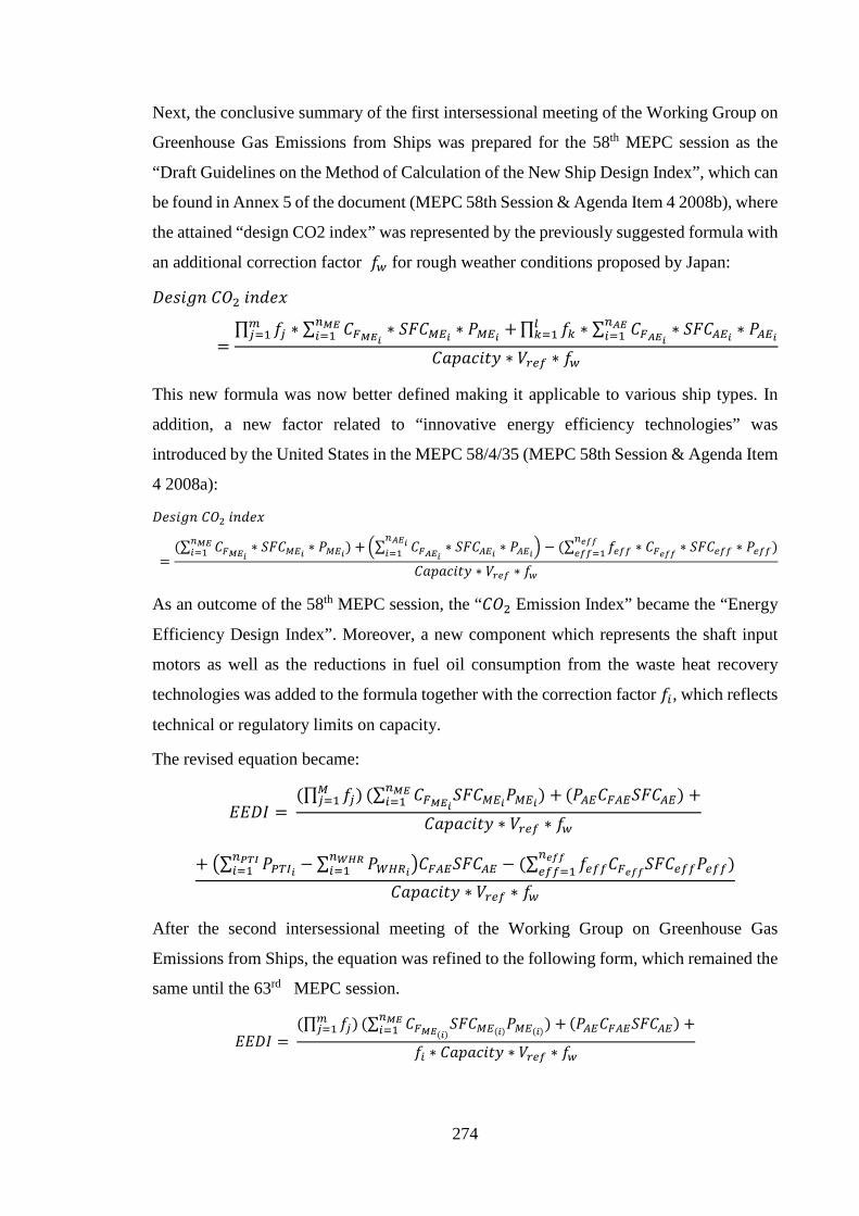
274
Next, the conclusive summary of the first intersessional meeting of the Working Group on
Greenhouse Gas Emissions from Ships was prepared for the 58th MEPC session as the
“Draft Guidelines on the Method of Calculation of the New Ship Design Index”, which can
be found in Annex 5 of the document (MEPC 58th Session & Agenda Item 4 2008b), where
the attained “design CO2 index” was represented by the previously suggested formula with
an additional correction factor 𝑓𝑓𝑤𝑤 for rough weather conditions proposed by Japan:
𝐷𝐷𝑒𝑒𝑔𝑔𝑖𝑖𝑔𝑔𝑛𝑛 𝐶𝐶𝐶𝐶2 𝑖𝑖𝑛𝑛𝑑𝑑𝑒𝑒𝑥𝑥
=∏ 𝑓𝑓𝑗𝑗𝑚𝑚𝑗𝑗=1 ∗ ∑ 𝐶𝐶𝐹𝐹𝑀𝑀𝑀𝑀𝑖𝑖
∗ 𝑆𝑆𝑆𝑆𝐶𝐶𝑀𝑀𝐸𝐸𝑖𝑖 ∗ 𝑃𝑃𝑀𝑀𝐸𝐸𝑖𝑖 +𝐴𝐴𝑀𝑀𝑀𝑀𝐴𝐴=1 ∏ 𝑓𝑓𝑘𝑘𝑙𝑙
𝑘𝑘=1 ∗ ∑ 𝐶𝐶𝐹𝐹𝐴𝐴𝑀𝑀𝑖𝑖 ∗ 𝑆𝑆𝑆𝑆𝐶𝐶𝐴𝐴𝐸𝐸𝑖𝑖 ∗ 𝑃𝑃𝐴𝐴𝐸𝐸𝑖𝑖𝐴𝐴𝐴𝐴𝑀𝑀𝐴𝐴=1
𝐶𝐶𝐻𝐻𝐶𝐶𝐻𝐻𝐶𝐶𝑖𝑖𝐶𝐶𝐶𝐶 ∗ 𝑁𝑁𝑟𝑟𝐴𝐴𝑟𝑟 ∗ 𝑓𝑓𝑤𝑤
This new formula was now better defined making it applicable to various ship types. In
addition, a new factor related to “innovative energy efficiency technologies” was
introduced by the United States in the MEPC 58/4/35 (MEPC 58th Session & Agenda Item
4 2008a):
𝐷𝐷𝑒𝑒𝑔𝑔𝑖𝑖𝑔𝑔𝑛𝑛 𝐶𝐶𝐶𝐶2 𝑖𝑖𝑛𝑛𝑑𝑑𝑒𝑒𝑥𝑥
=(∑ 𝐶𝐶𝐹𝐹𝑀𝑀𝑀𝑀𝑖𝑖
∗ 𝑆𝑆𝑆𝑆𝐶𝐶𝑀𝑀𝐸𝐸𝑖𝑖 ∗ 𝑃𝑃𝑀𝑀𝐸𝐸𝑖𝑖) +𝐴𝐴𝑀𝑀𝑀𝑀𝐴𝐴=1 ∑ 𝐶𝐶𝐹𝐹𝐴𝐴𝑀𝑀𝑖𝑖 ∗ 𝑆𝑆𝑆𝑆𝐶𝐶𝐴𝐴𝐸𝐸𝑖𝑖 ∗ 𝑃𝑃𝐴𝐴𝐸𝐸𝑖𝑖
𝐴𝐴𝐴𝐴𝑀𝑀𝑖𝑖𝐴𝐴=1 − (∑ 𝑓𝑓𝐴𝐴𝑟𝑟𝑟𝑟 ∗ 𝐶𝐶𝐹𝐹𝑟𝑟𝑟𝑟𝑟𝑟 ∗ 𝑆𝑆𝑆𝑆𝐶𝐶𝐴𝐴𝑟𝑟𝑟𝑟 ∗ 𝑃𝑃𝐴𝐴𝑟𝑟𝑟𝑟
𝐴𝐴𝑟𝑟𝑟𝑟𝑟𝑟𝐴𝐴𝑟𝑟𝑟𝑟=1 )
𝐶𝐶𝐻𝐻𝐶𝐶𝐻𝐻𝐶𝐶𝑖𝑖𝐶𝐶𝐶𝐶 ∗ 𝑁𝑁𝑟𝑟𝐴𝐴𝑟𝑟 ∗ 𝑓𝑓𝑤𝑤
As an outcome of the 58th MEPC session, the “𝐶𝐶𝐶𝐶2 Emission Index” became the “Energy
Efficiency Design Index”. Moreover, a new component which represents the shaft input
motors as well as the reductions in fuel oil consumption from the waste heat recovery
technologies was added to the formula together with the correction factor 𝑓𝑓𝐴𝐴, which reflects
technical or regulatory limits on capacity.
The revised equation became:
𝐸𝐸𝐸𝐸𝐷𝐷𝐸𝐸 = (∏ 𝑓𝑓𝑗𝑗)𝑀𝑀
𝑗𝑗=1 (∑ 𝐶𝐶𝐹𝐹𝑀𝑀𝑀𝑀𝑖𝑖𝑆𝑆𝑆𝑆𝐶𝐶𝑀𝑀𝐸𝐸𝑖𝑖𝑃𝑃𝑀𝑀𝐸𝐸𝑖𝑖) +𝐴𝐴𝑀𝑀𝑀𝑀
𝐴𝐴=1 (𝑃𝑃𝐴𝐴𝐸𝐸𝐶𝐶𝐹𝐹𝐴𝐴𝐸𝐸𝑆𝑆𝑆𝑆𝐶𝐶𝐴𝐴𝐸𝐸) +
𝐶𝐶𝐻𝐻𝐶𝐶𝐻𝐻𝐶𝐶𝑖𝑖𝐶𝐶𝐶𝐶 ∗ 𝑁𝑁𝑟𝑟𝐴𝐴𝑟𝑟 ∗ 𝑓𝑓𝑤𝑤
+ ∑ 𝑃𝑃𝑃𝑃𝑇𝑇𝐴𝐴𝑖𝑖 − ∑ 𝑃𝑃𝑊𝑊𝐻𝐻𝑅𝑅𝑖𝑖𝐴𝐴𝑊𝑊𝐻𝐻𝑊𝑊𝐴𝐴=1
𝐴𝐴𝑃𝑃𝑂𝑂𝑃𝑃𝐴𝐴=1 𝐶𝐶𝐹𝐹𝐴𝐴𝐸𝐸𝑆𝑆𝑆𝑆𝐶𝐶𝐴𝐴𝐸𝐸 − (∑ 𝑓𝑓𝐴𝐴𝑟𝑟𝑟𝑟𝐶𝐶𝐹𝐹𝑟𝑟𝑟𝑟𝑟𝑟𝑆𝑆𝑆𝑆𝐶𝐶𝐴𝐴𝑟𝑟𝑟𝑟𝑃𝑃𝐴𝐴𝑟𝑟𝑟𝑟
𝐴𝐴𝑟𝑟𝑟𝑟𝑟𝑟𝐴𝐴𝑟𝑟𝑟𝑟=1 )
𝐶𝐶𝐻𝐻𝐶𝐶𝐻𝐻𝐶𝐶𝑖𝑖𝐶𝐶𝐶𝐶 ∗ 𝑁𝑁𝑟𝑟𝐴𝐴𝑟𝑟 ∗ 𝑓𝑓𝑤𝑤
After the second intersessional meeting of the Working Group on Greenhouse Gas
Emissions from Ships, the equation was refined to the following form, which remained the
same until the 63rd MEPC session.
𝐸𝐸𝐸𝐸𝐷𝐷𝐸𝐸 = (∏ 𝑓𝑓𝑗𝑗)𝑚𝑚
𝑗𝑗=1 (∑ 𝐶𝐶𝐹𝐹𝑀𝑀𝑀𝑀(𝑖𝑖)𝑆𝑆𝑆𝑆𝐶𝐶𝑀𝑀𝐸𝐸(𝑖𝑖)𝑃𝑃𝑀𝑀𝐸𝐸(𝑖𝑖)) +𝐴𝐴𝑀𝑀𝑀𝑀
𝐴𝐴=1 (𝑃𝑃𝐴𝐴𝐸𝐸𝐶𝐶𝐹𝐹𝐴𝐴𝐸𝐸𝑆𝑆𝑆𝑆𝐶𝐶𝐴𝐴𝐸𝐸) +
𝑓𝑓𝐴𝐴 ∗ 𝐶𝐶𝐻𝐻𝐶𝐶𝐻𝐻𝐶𝐶𝑖𝑖𝐶𝐶𝐶𝐶 ∗ 𝑁𝑁𝑟𝑟𝐴𝐴𝑟𝑟 ∗ 𝑓𝑓𝑤𝑤

275
+∏ 𝑓𝑓𝑗𝑗𝑚𝑚𝑗𝑗=1 ∗ ∑ 𝑃𝑃𝑃𝑃𝑇𝑇𝐴𝐴(𝑖𝑖) −∑ 𝑓𝑓𝐴𝐴𝑟𝑟𝑟𝑟(𝑖𝑖)𝑃𝑃𝐴𝐴𝐸𝐸𝑟𝑟𝑟𝑟𝑟𝑟(𝑖𝑖)
𝐴𝐴𝑟𝑟𝑟𝑟𝑟𝑟𝐴𝐴=1
𝐴𝐴𝑃𝑃𝑂𝑂𝑃𝑃𝐴𝐴=1 𝐶𝐶𝐹𝐹𝐴𝐴𝑀𝑀𝑆𝑆𝑆𝑆𝐶𝐶𝐴𝐴𝐸𝐸 − (∑ 𝑓𝑓𝐴𝐴𝑟𝑟𝑟𝑟(𝑖𝑖)𝑃𝑃𝐴𝐴𝑟𝑟𝑟𝑟(𝑖𝑖)𝐶𝐶𝐹𝐹𝑀𝑀𝑀𝑀𝑆𝑆𝑆𝑆𝐶𝐶𝑀𝑀𝐸𝐸
𝐴𝐴𝑟𝑟𝑟𝑟𝑟𝑟𝐴𝐴𝑟𝑟𝑟𝑟=1 )
𝑓𝑓𝐴𝐴 ∗ 𝐶𝐶𝐻𝐻𝐶𝐶𝐻𝐻𝐶𝐶𝑖𝑖𝐶𝐶𝐶𝐶 ∗ 𝑁𝑁𝑟𝑟𝐴𝐴𝑟𝑟 ∗ 𝑓𝑓𝑤𝑤
Then, the updated formulation of the EEDI index, with added cubic capacity correction
factor 𝑓𝑓𝑐𝑐, was adopted during 63rd MEPC session and then published as “2012 Guidelines
on the Method of Calculation of the Attained Energy Efficiency Design Index (EEDI) for
New Ships” (MEPC 212(63) Annex 8 2012):
𝐸𝐸𝐸𝐸𝐷𝐷𝐸𝐸 = (∏ 𝑓𝑓𝑗𝑗)𝐴𝐴
𝑗𝑗=1 (∑ 𝑃𝑃𝑀𝑀𝐸𝐸(𝑖𝑖)𝐶𝐶𝐹𝐹𝑀𝑀𝑀𝑀(𝑖𝑖)𝑆𝑆𝑆𝑆𝐶𝐶𝑀𝑀𝐸𝐸(𝑖𝑖)) +𝐴𝐴𝑀𝑀𝑀𝑀
𝐴𝐴=1 𝑃𝑃𝐴𝐴𝐸𝐸𝐶𝐶𝐹𝐹𝐴𝐴𝑀𝑀𝑆𝑆𝑆𝑆𝐶𝐶𝐴𝐴𝐸𝐸 +
𝑓𝑓𝐴𝐴 ∗ 𝑓𝑓𝑐𝑐 ∗ 𝐶𝐶𝐻𝐻𝐶𝐶𝐻𝐻𝐶𝐶𝑖𝑖𝐶𝐶𝐶𝐶 ∗ 𝑁𝑁𝑟𝑟𝐴𝐴𝑟𝑟 ∗ 𝑓𝑓𝑤𝑤
+∏ 𝑓𝑓𝑗𝑗𝐴𝐴𝑗𝑗=1 ∗ ∑ 𝑃𝑃𝑃𝑃𝑇𝑇𝐴𝐴(𝑖𝑖) −∑ 𝑓𝑓𝐴𝐴𝑟𝑟𝑟𝑟(𝑖𝑖)𝑃𝑃𝐴𝐴𝐸𝐸𝑟𝑟𝑟𝑟𝑟𝑟(𝑖𝑖)
𝐴𝐴𝑟𝑟𝑟𝑟𝑟𝑟𝐴𝐴=1
𝐴𝐴𝑃𝑃𝑂𝑂𝑃𝑃𝐴𝐴=1 𝐶𝐶𝐹𝐹𝐴𝐴𝑀𝑀𝑆𝑆𝑆𝑆𝐶𝐶𝐴𝐴𝐸𝐸 − (∑ 𝑓𝑓𝐴𝐴𝑟𝑟𝑟𝑟(𝑖𝑖)𝑃𝑃𝐴𝐴𝑟𝑟𝑟𝑟(𝑖𝑖)𝐶𝐶𝐹𝐹𝑀𝑀𝑀𝑀𝑆𝑆𝑆𝑆𝐶𝐶𝑀𝑀𝐸𝐸
𝐴𝐴𝑟𝑟𝑟𝑟𝑟𝑟𝐴𝐴𝑟𝑟𝑟𝑟=1 )
𝑓𝑓𝐴𝐴 ∗ 𝑓𝑓𝑐𝑐 ∗ 𝐶𝐶𝐻𝐻𝐶𝐶𝐻𝐻𝐶𝐶𝑖𝑖𝐶𝐶𝐶𝐶 ∗ 𝑁𝑁𝑟𝑟𝐴𝐴𝑟𝑟 ∗ 𝑓𝑓𝑤𝑤
The most recent EEDI formula has been adopted during the 66th MEPC session and, as
previously stated, is available in Annex 5, MEPC.245 (66) “2014 Guidelines on the Method
of Calculation of the Attained Energy Efficiency Design Index (EEDI) for New Ships”
supported by newly developed “Industry guidelines on calculation and verification of the
EEDI”, which have been adopted during the recent 68th MEPC session (MEPC 68/INF.30
2015).
The final EEDI formula additionally includes the correction factor 𝑓𝑓𝑙𝑙 designed for general
cargo ships equipped with cranes and other cargo-related gear:
𝐸𝐸𝐸𝐸𝐷𝐷𝐸𝐸 = (∏ 𝑓𝑓𝑗𝑗)𝐴𝐴
𝑗𝑗=1 (∑ 𝑃𝑃𝑀𝑀𝐸𝐸(𝑖𝑖)𝐶𝐶𝐹𝐹𝑀𝑀𝑀𝑀(𝑖𝑖)𝑆𝑆𝑆𝑆𝐶𝐶𝑀𝑀𝐸𝐸(𝑖𝑖)) +𝐴𝐴𝑀𝑀𝑀𝑀
𝐴𝐴=1 𝑃𝑃𝐴𝐴𝐸𝐸𝐶𝐶𝐹𝐹𝐴𝐴𝑀𝑀𝑆𝑆𝑆𝑆𝐶𝐶𝐴𝐴𝐸𝐸 +
𝑓𝑓𝐴𝐴 ∗ 𝑓𝑓𝑐𝑐 ∗ 𝑓𝑓𝑙𝑙 ∗ 𝐶𝐶𝐻𝐻𝐶𝐶𝐻𝐻𝐶𝐶𝑖𝑖𝐶𝐶𝐶𝐶 ∗ 𝑁𝑁𝑟𝑟𝐴𝐴𝑟𝑟 ∗ 𝑓𝑓𝑤𝑤
+∏ 𝑓𝑓𝑗𝑗𝐴𝐴𝑗𝑗=1 ∗ ∑ 𝑃𝑃𝑃𝑃𝑇𝑇𝐴𝐴(𝑖𝑖) −∑ 𝑓𝑓𝐴𝐴𝑟𝑟𝑟𝑟(𝑖𝑖)𝑃𝑃𝐴𝐴𝐸𝐸𝑟𝑟𝑟𝑟𝑟𝑟(𝑖𝑖)
𝐴𝐴𝑟𝑟𝑟𝑟𝑟𝑟𝐴𝐴=1
𝐴𝐴𝑃𝑃𝑂𝑂𝑃𝑃𝐴𝐴=1 𝐶𝐶𝐹𝐹𝐴𝐴𝑀𝑀𝑆𝑆𝑆𝑆𝐶𝐶𝐴𝐴𝐸𝐸 − (∑ 𝑓𝑓𝐴𝐴𝑟𝑟𝑟𝑟(𝑖𝑖)𝑃𝑃𝐴𝐴𝑟𝑟𝑟𝑟(𝑖𝑖)𝐶𝐶𝐹𝐹𝑀𝑀𝑀𝑀𝑆𝑆𝑆𝑆𝐶𝐶𝑀𝑀𝐸𝐸
𝐴𝐴𝑟𝑟𝑟𝑟𝑟𝑟𝐴𝐴𝑟𝑟𝑟𝑟=1 )
𝑓𝑓𝐴𝐴 ∗ 𝑓𝑓𝑐𝑐 ∗ 𝑓𝑓𝑙𝑙 ∗ 𝐶𝐶𝐻𝐻𝐶𝐶𝐻𝐻𝐶𝐶𝑖𝑖𝐶𝐶𝐶𝐶 ∗ 𝑁𝑁𝑟𝑟𝐴𝐴𝑟𝑟 ∗ 𝑓𝑓𝑤𝑤
However, the EEDI formula development has been continuously ongoing as it still has
some deficiencies such as it is not applicable to a ship having diesel-electric propulsion,
turbine propulsion or hybrid propulsion system, except for cruise passenger ships and LNG
carriers.
Explanation of Terms
• Conversion factors (𝐶𝐶𝐹𝐹𝑀𝑀𝑀𝑀 and 𝐶𝐶𝐹𝐹𝐴𝐴𝑀𝑀)
Non-dimensional conversion factors are given for the following categories of fuels used in
the marine industry: diesel/gas oil, light fuel oil (LFO), heavy fuel oil (HFO), liquefied
petroleum gas (LPG) in form of butane, LPG in form of propane, liquefied natural gas
276
(LNG), methanol and ethanol. These conversion factors, listed in the (IMO 2014a), define
an equivalent mass of 𝐶𝐶𝐶𝐶2 normally emitted during the complete combustion of a given
mass of fuel. The type of fuel used in the calculation of EEDI should be the same as the
fuel burned for the estimation of the specific fuel consumption (SFC) in the Engine
International Air Pollution Prevention (EIAPP) certificate.
• Certified specific fuel consumption (𝑆𝑆𝑆𝑆𝐶𝐶𝑀𝑀𝐸𝐸 and 𝑆𝑆𝑆𝑆𝐶𝐶𝐴𝐴𝐸𝐸) Certified specific fuel consumption (SFC) is divided into two categories: main engine and
auxiliary engine fuel consumption. Main engine fuel consumption is the specific fuel
consumption measured in g/kWh reported in the EIAPP certificate for the parent engine in
accordance with the 𝑁𝑁𝐶𝐶𝑋𝑋 Technical Code at 75 percent of the Maximum Continuous Rating
(MCR). Auxiliary engine fuel consumption is the fuel consumption reported on the parent
engine’s EIAPP certificate at 50 percent of the MCR. If different sized auxiliary engines
are used, a single SFC is entered into the equation by taking the weighted average of the
different engines.
• Power (𝑃𝑃𝑀𝑀𝐸𝐸 ,𝑃𝑃𝐴𝐴𝐸𝐸 ,𝑃𝑃𝑃𝑃𝑇𝑇𝐴𝐴) The main engine power 𝑃𝑃𝑀𝑀𝐸𝐸 used in the EEDI calculation is 75 percent of the MCR of the
engine measured in kW minus the output of any shaft generators and should be calculated
as follows:
𝑃𝑃𝑀𝑀𝐸𝐸(𝑖𝑖)
𝐴𝐴𝑀𝑀𝑀𝑀
𝐴𝐴=1
= 0.75 ∗ 𝑁𝑁𝐶𝐶𝐵𝐵𝑀𝑀𝐸𝐸(𝑖𝑖) −𝑃𝑃𝑃𝑃𝑇𝑇𝑂𝑂(𝑖𝑖)
where 𝑃𝑃𝑃𝑃𝑇𝑇𝑂𝑂(𝑖𝑖) is the 75 percent of the rated electrical output power of each shaft generator
defined as 0.75 ∗ ∑𝑃𝑃𝑃𝑃𝑇𝑇𝑂𝑂(𝑖𝑖) ≤ 𝑃𝑃𝐴𝐴𝐸𝐸
The power from auxiliary engines 𝑃𝑃𝐴𝐴𝐸𝐸 is determined by an empirical formula representing
the hotel load and electrical needs for propulsion systems and machinery. Auxiliary power
is taken as a function of the MCR of the main engine(s). The second formula is adjusted
for vessels that have smaller propulsion engines with the installed MCR less than 10,000
kW. Additional shaft motor 𝑃𝑃𝑃𝑃𝑇𝑇𝐴𝐴 inputs are given at 75 percent of the rated power
consumption divided by the weighted average of the efficiency of the generators.
𝑃𝑃𝐴𝐴𝐸𝐸(∑𝑀𝑀𝐶𝐶𝑊𝑊𝑀𝑀𝑀𝑀(𝑖𝑖)≥ 10000 𝑘𝑘𝑊𝑊) = 0.025 ∗ ∑ 𝑁𝑁𝐶𝐶𝐵𝐵𝑀𝑀𝐸𝐸(𝑖𝑖) +
∑ 𝑃𝑃𝑃𝑃𝑂𝑂𝑃𝑃(𝑖𝑖)𝑛𝑛𝑃𝑃𝑂𝑂𝑃𝑃𝑖𝑖=1
0.75𝐴𝐴𝑀𝑀𝑀𝑀𝐴𝐴=1 + 250
𝑃𝑃𝐴𝐴𝐸𝐸(∑𝑀𝑀𝐶𝐶𝑊𝑊𝑀𝑀𝑀𝑀(𝑖𝑖)≤ 10000 𝑘𝑘𝑊𝑊) = 0.05 ∗ ∑ 𝑁𝑁𝐶𝐶𝐵𝐵𝑀𝑀𝐸𝐸(𝑖𝑖) +
∑ 𝑃𝑃𝑃𝑃𝑂𝑂𝑃𝑃(𝑖𝑖)𝑛𝑛𝑃𝑃𝑂𝑂𝑃𝑃𝑖𝑖=1
0.75𝐴𝐴𝑀𝑀𝑀𝑀𝐴𝐴=1
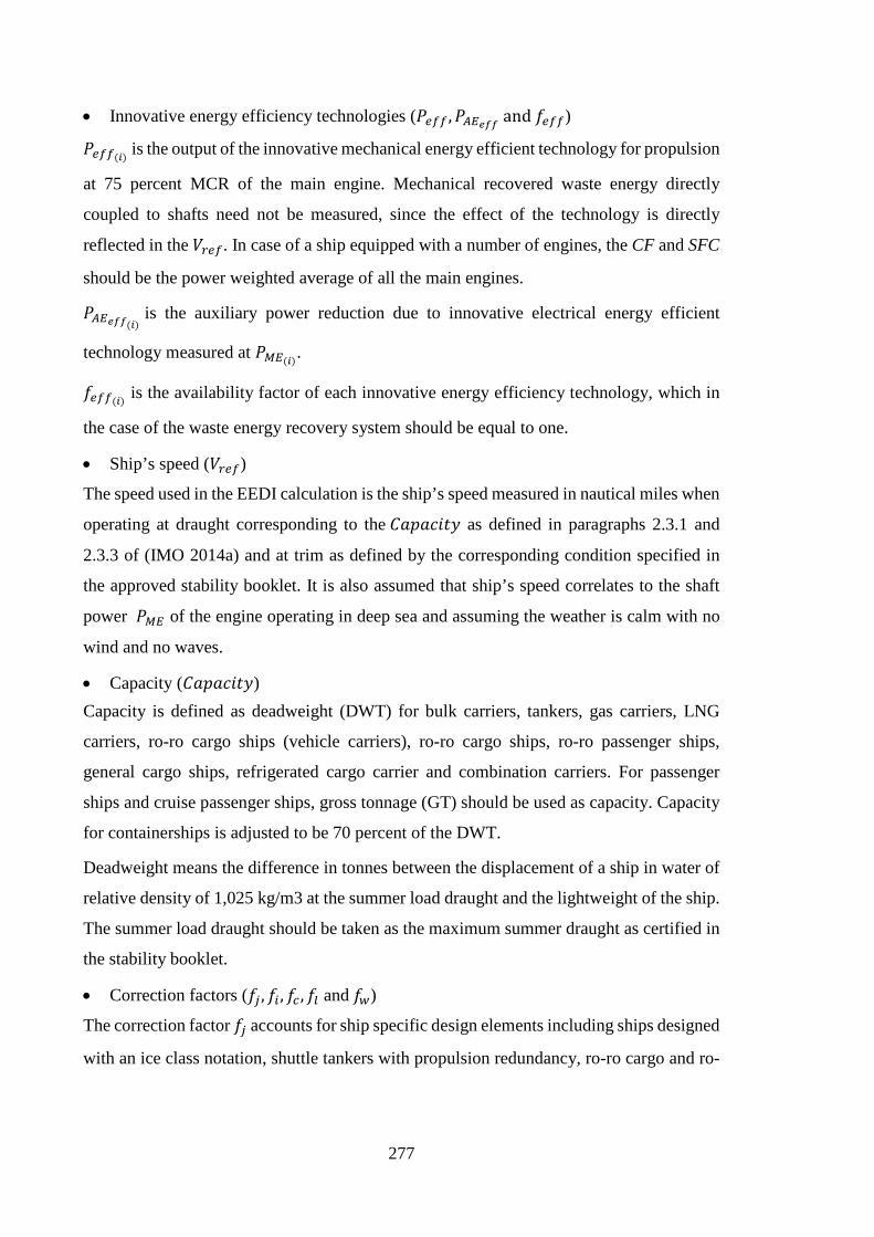
277
• Innovative energy efficiency technologies (𝑃𝑃𝐴𝐴𝑟𝑟𝑟𝑟 ,𝑃𝑃𝐴𝐴𝐸𝐸𝑟𝑟𝑟𝑟𝑟𝑟 and 𝑓𝑓𝐴𝐴𝑟𝑟𝑟𝑟)
𝑃𝑃𝐴𝐴𝑟𝑟𝑟𝑟(𝑖𝑖) is the output of the innovative mechanical energy efficient technology for propulsion
at 75 percent MCR of the main engine. Mechanical recovered waste energy directly
coupled to shafts need not be measured, since the effect of the technology is directly
reflected in the 𝑁𝑁𝑟𝑟𝐴𝐴𝑟𝑟. In case of a ship equipped with a number of engines, the CF and SFC
should be the power weighted average of all the main engines.
𝑃𝑃𝐴𝐴𝐸𝐸𝑟𝑟𝑟𝑟𝑟𝑟(𝑖𝑖) is the auxiliary power reduction due to innovative electrical energy efficient
technology measured at 𝑃𝑃𝑀𝑀𝐸𝐸(𝑖𝑖).
𝑓𝑓𝐴𝐴𝑟𝑟𝑟𝑟(𝑖𝑖) is the availability factor of each innovative energy efficiency technology, which in
the case of the waste energy recovery system should be equal to one.
• Ship’s speed (𝑁𝑁𝑟𝑟𝐴𝐴𝑟𝑟)
The speed used in the EEDI calculation is the ship’s speed measured in nautical miles when
operating at draught corresponding to the 𝐶𝐶𝐻𝐻𝐶𝐶𝐻𝐻𝐶𝐶𝑖𝑖𝐶𝐶𝐶𝐶 as defined in paragraphs 2.3.1 and
2.3.3 of (IMO 2014a) and at trim as defined by the corresponding condition specified in
the approved stability booklet. It is also assumed that ship’s speed correlates to the shaft
power 𝑃𝑃𝑀𝑀𝐸𝐸 of the engine operating in deep sea and assuming the weather is calm with no
wind and no waves.
• Capacity (𝐶𝐶𝐻𝐻𝐶𝐶𝐻𝐻𝐶𝐶𝑖𝑖𝐶𝐶𝐶𝐶) Capacity is defined as deadweight (DWT) for bulk carriers, tankers, gas carriers, LNG
carriers, ro-ro cargo ships (vehicle carriers), ro-ro cargo ships, ro-ro passenger ships,
general cargo ships, refrigerated cargo carrier and combination carriers. For passenger
ships and cruise passenger ships, gross tonnage (GT) should be used as capacity. Capacity
for containerships is adjusted to be 70 percent of the DWT.
Deadweight means the difference in tonnes between the displacement of a ship in water of
relative density of 1,025 kg/m3 at the summer load draught and the lightweight of the ship.
The summer load draught should be taken as the maximum summer draught as certified in
the stability booklet.
• Correction factors (𝑓𝑓𝑗𝑗 ,𝑓𝑓𝐴𝐴 ,𝑓𝑓𝑐𝑐 ,𝑓𝑓𝑙𝑙 and 𝑓𝑓𝑤𝑤)
The correction factor 𝑓𝑓𝑗𝑗 accounts for ship specific design elements including ships designed
with an ice class notation, shuttle tankers with propulsion redundancy, ro-ro cargo and ro-
278
ro passenger ships and general cargo ships, which calculation details can be found in section
2.8 of (IMO 2014a). For other ship types, 𝑓𝑓𝑗𝑗 should be taken as one.
The correction factor 𝑓𝑓𝐴𝐴 is related to any technical or regulatory limit on capacity in case of
ice-classed ships, ships with specific voluntary enhancements or bulk currier and oil tankers
built in accordance with the Common Structural Rules (CSR) of the classification societies
and assigned the class notation CSR. The calculation process of 𝑓𝑓𝐴𝐴 is explained in section
2.11 of (IMO 2014a). For other ship types, 𝑓𝑓𝐴𝐴 should be taken as one.
The factor 𝑓𝑓𝑐𝑐 is the cubic capacity correction factor that should be added to EEDI
calculations in case of chemical tankers, gas carriers with direct diesel driven propulsion
system constructed or adapted to use for the carriage in bulk of liquefied natural gas and
ro-ro passenger ships with a DWT/GT ratio of less than 0.25 in accordance to section 2.12
of (IMO 2014a). For other ship types, 𝑓𝑓𝑐𝑐 should be taken as one.
𝑓𝑓𝑙𝑙 is the factor for general cargo ships equipped with cranes and other cargo-related gear to
compensate a loss of deadweight of the ship calculated in accordance to 2.13 of (IMO
2014a) or taken as one if not applicable.
𝑓𝑓𝑤𝑤 is a factor representing the decrease in speed in certain sea conditions of wave height,
wave frequency and wind speed (Beaufort Scale 6), and, if calculated according to the
(MEPC.1/Circ.796 2012), the value for attained EEDI should be referred as 𝐸𝐸𝐸𝐸𝐷𝐷𝐸𝐸𝑊𝑊𝐴𝐴𝑔𝑔𝐴𝐴ℎ𝐴𝐴𝑟𝑟.
This weather correction factor can be determined by conducting the ship specific simulation
on its performance at representative sea conditions. Otherwise, if the simulation is not
available, 𝑓𝑓𝑤𝑤 can be estimated using “standard 𝑓𝑓𝑤𝑤” curve, which is only provided for bulk
carrier, tanker and container ship as specified below:
𝑓𝑓𝑤𝑤 = 𝐻𝐻 ∗ ln(𝐶𝐶𝐻𝐻𝐶𝐶𝐻𝐻𝐶𝐶𝑖𝑖𝐶𝐶𝐶𝐶) + 𝑙𝑙
where 𝐻𝐻 and 𝑙𝑙 are the parameters given in Table A 1.
Table A 1. Parameters for determination of standard 𝑓𝑓𝑤𝑤 value.
Ship Type A b
Bulk carrier 0.0429 0.294
Tanker 0.0238 0.526
Container ship 0.0208 0.633
It is important to note, that inclusion of 𝑓𝑓𝑤𝑤 is a voluntary option and should be taken as one
in case of a conventional EEDI estimation process.
279
EEDI Reference Line Methodology
A methodology used for development of the reference line curves for the EEDI has been
introduced by Denmark and, for the first time, suggested in the MEPC 58/4/8. Then, in
GHG-WG 2/2/7, Denmark updated the methodology to reflect the latest update of the EEDI
formula. The most recent version of the EEDI reference line calculation methodology has
been adopted on 17th of May 2013. The document is titled “2013 guidelines for calculation
of reference lines for use with the energy efficiency design index (EEDI)”(IMO 2013).
The reference lines are established for each of the following ship types: bulk carrier, gas
carrier, tanker, container ship, general cargo ship, refrigerated cargo carrier, combination
carrier, ro-ro cargo ship, ro-ro cargo ship (vehicle), ro-ro passenger ship and LNG carrier.
It is noted that a method of calculating reference lines has not been established for
passenger ships other than cruise passenger ship having non-conventional propulsion.
Generally, a reference lines defined as a curve representing an average index value fitted
on a set of individual index values for a defined group of ships. The data used for the
calculation of the reference line is derived from the IHS Fairplay vessel database of all
ships of a particular type that were built in the period the years 1999-2009. In order to get
baseline EEDI for each data point, simplifying assumptions were required to adjust for
missing information in the IHSF database. Some of the simplifying assumptions are:
• Conversion factors (𝐶𝐶𝐹𝐹𝑀𝑀𝑀𝑀 and 𝐶𝐶𝐹𝐹𝐴𝐴𝑀𝑀)
A single fuel type, the heavy fuel oil (HFO), is assumed to be used in all engines, both
propulsion and auxiliary. Therefore, the carbon emission factor is constant for all engines
and equals to 3.1144 𝑔𝑔𝐶𝐶𝑂𝑂2/𝑔𝑔𝑟𝑟𝑅𝑅𝐴𝐴𝑙𝑙.
• Certified specific fuel consumption (𝑆𝑆𝑆𝑆𝐶𝐶𝑀𝑀𝐸𝐸 and 𝑆𝑆𝑆𝑆𝐶𝐶𝐴𝐴𝐸𝐸) As the specific fuel consumption data was not always available in the IHSF database, a
constant value of 190 g/ kW‐hr has been applied to all propulsion engines. Auxiliary
engine fuel consumption is also assumed to be constant and has been taken
as 215 g/ kW‐h.
• Power (𝑃𝑃𝑀𝑀𝐸𝐸 ,𝑃𝑃𝐴𝐴𝐸𝐸) Similarly to the EEDI formula, 𝑃𝑃𝑀𝑀𝐸𝐸 , is taken as 75 percent of listed MCR in the database.
𝑃𝑃𝐴𝐴𝐸𝐸 has been estimated using the same empirical formula as for the EEDI calculations.
• Speed (𝑁𝑁𝑟𝑟𝐴𝐴𝑟𝑟)
𝑁𝑁𝑟𝑟𝐴𝐴𝑟𝑟 used for the estimation of the reference line is the speed listed in the IHSF database.
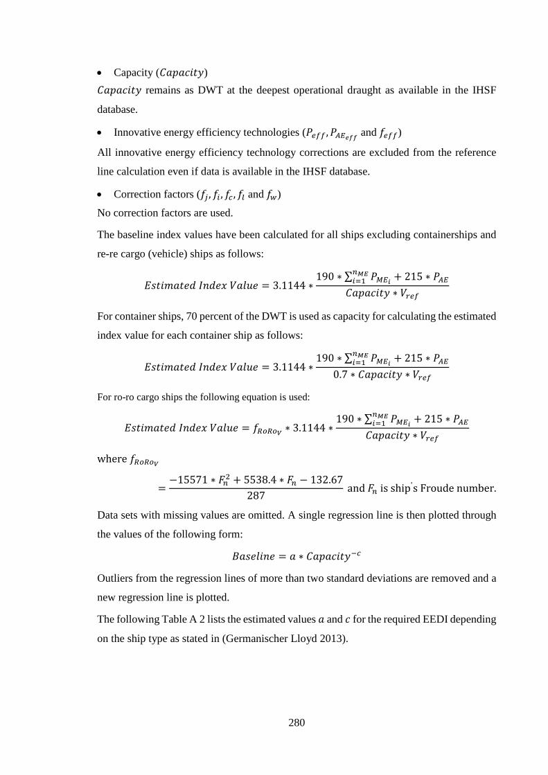
280
• Capacity (𝐶𝐶𝐻𝐻𝐶𝐶𝐻𝐻𝐶𝐶𝑖𝑖𝐶𝐶𝐶𝐶) 𝐶𝐶𝐻𝐻𝐶𝐶𝐻𝐻𝐶𝐶𝑖𝑖𝐶𝐶𝐶𝐶 remains as DWT at the deepest operational draught as available in the IHSF
database.
• Innovative energy efficiency technologies (𝑃𝑃𝐴𝐴𝑟𝑟𝑟𝑟 ,𝑃𝑃𝐴𝐴𝐸𝐸𝑟𝑟𝑟𝑟𝑟𝑟 and 𝑓𝑓𝐴𝐴𝑟𝑟𝑟𝑟)
All innovative energy efficiency technology corrections are excluded from the reference
line calculation even if data is available in the IHSF database.
• Correction factors (𝑓𝑓𝑗𝑗 ,𝑓𝑓𝐴𝐴 ,𝑓𝑓𝑐𝑐 ,𝑓𝑓𝑙𝑙 and 𝑓𝑓𝑤𝑤)
No correction factors are used.
The baseline index values have been calculated for all ships excluding containerships and
re-re cargo (vehicle) ships as follows:
𝐸𝐸𝑔𝑔𝐶𝐶𝑖𝑖𝑛𝑛𝐻𝐻𝐶𝐶𝑒𝑒𝑑𝑑 𝐸𝐸𝑛𝑛𝑑𝑑𝑒𝑒𝑥𝑥 𝑁𝑁𝐻𝐻𝑙𝑙𝑢𝑢𝑒𝑒 = 3.1144 ∗190 ∗ ∑ 𝑃𝑃𝑀𝑀𝐸𝐸𝑖𝑖 + 215 ∗ 𝑃𝑃𝐴𝐴𝐸𝐸
𝐴𝐴𝑀𝑀𝑀𝑀𝐴𝐴=1𝐶𝐶𝐻𝐻𝐶𝐶𝐻𝐻𝐶𝐶𝑖𝑖𝐶𝐶𝐶𝐶 ∗ 𝑁𝑁𝑟𝑟𝐴𝐴𝑟𝑟
For container ships, 70 percent of the DWT is used as capacity for calculating the estimated
index value for each container ship as follows:
𝐸𝐸𝑔𝑔𝐶𝐶𝑖𝑖𝑛𝑛𝐻𝐻𝐶𝐶𝑒𝑒𝑑𝑑 𝐸𝐸𝑛𝑛𝑑𝑑𝑒𝑒𝑥𝑥 𝑁𝑁𝐻𝐻𝑙𝑙𝑢𝑢𝑒𝑒 = 3.1144 ∗190 ∗ ∑ 𝑃𝑃𝑀𝑀𝐸𝐸𝑖𝑖 + 215 ∗ 𝑃𝑃𝐴𝐴𝐸𝐸
𝐴𝐴𝑀𝑀𝑀𝑀𝐴𝐴=1
0.7 ∗ 𝐶𝐶𝐻𝐻𝐶𝐶𝐻𝐻𝐶𝐶𝑖𝑖𝐶𝐶𝐶𝐶 ∗ 𝑁𝑁𝑟𝑟𝐴𝐴𝑟𝑟
For ro-ro cargo ships the following equation is used:
𝐸𝐸𝑔𝑔𝐶𝐶𝑖𝑖𝑛𝑛𝐻𝐻𝐶𝐶𝑒𝑒𝑑𝑑 𝐸𝐸𝑛𝑛𝑑𝑑𝑒𝑒𝑥𝑥 𝑁𝑁𝐻𝐻𝑙𝑙𝑢𝑢𝑒𝑒 = 𝑓𝑓𝑅𝑅𝑏𝑏𝑅𝑅𝑏𝑏𝑉𝑉 ∗ 3.1144 ∗190 ∗ ∑ 𝑃𝑃𝑀𝑀𝐸𝐸𝑖𝑖 + 215 ∗ 𝑃𝑃𝐴𝐴𝐸𝐸
𝐴𝐴𝑀𝑀𝑀𝑀𝐴𝐴=1𝐶𝐶𝐻𝐻𝐶𝐶𝐻𝐻𝐶𝐶𝑖𝑖𝐶𝐶𝐶𝐶 ∗ 𝑁𝑁𝑟𝑟𝐴𝐴𝑟𝑟
where 𝑓𝑓𝑅𝑅𝑏𝑏𝑅𝑅𝑏𝑏𝑉𝑉
=−15571 ∗ 𝑆𝑆𝐴𝐴2 + 5538.4 ∗ 𝑆𝑆𝐴𝐴 − 132.67
287 and 𝑆𝑆𝐴𝐴 is ship's Froude number.
Data sets with missing values are omitted. A single regression line is then plotted through
the values of the following form:
𝐵𝐵𝐻𝐻𝑔𝑔𝑒𝑒𝑙𝑙𝑖𝑖𝑛𝑛𝑒𝑒 = 𝐻𝐻 ∗ 𝐶𝐶𝐻𝐻𝐶𝐶𝐻𝐻𝐶𝐶𝑖𝑖𝐶𝐶𝐶𝐶−𝑐𝑐
Outliers from the regression lines of more than two standard deviations are removed and a
new regression line is plotted.
The following Table A 2 lists the estimated values 𝐻𝐻 and 𝐶𝐶 for the required EEDI depending
on the ship type as stated in (Germanischer Lloyd 2013).
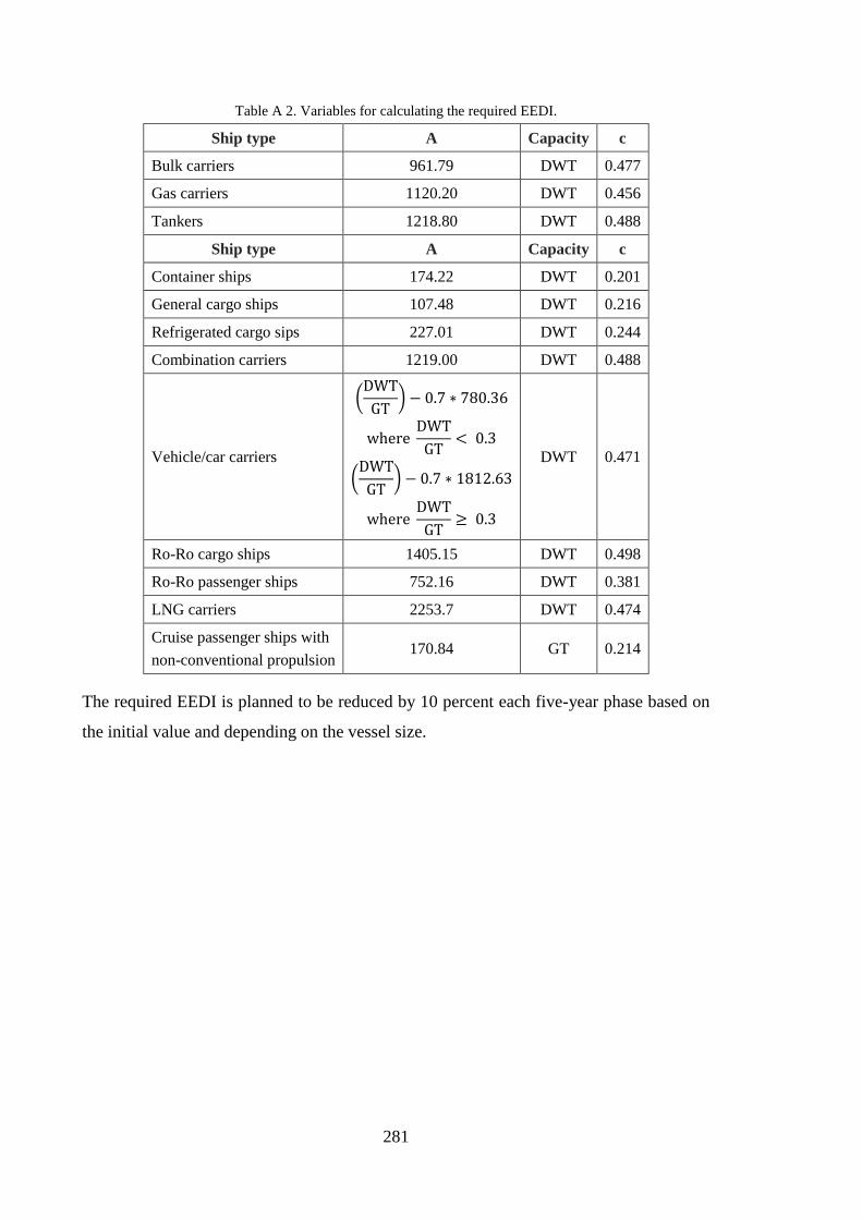
281
Table A 2. Variables for calculating the required EEDI.
Ship type A Capacity c
Bulk carriers 961.79 DWT 0.477
Gas carriers 1120.20 DWT 0.456
Tankers 1218.80 DWT 0.488
Ship type A Capacity c
Container ships 174.22 DWT 0.201
General cargo ships 107.48 DWT 0.216
Refrigerated cargo sips 227.01 DWT 0.244
Combination carriers 1219.00 DWT 0.488
Vehicle/car carriers
DWT
GT − 0.7 ∗ 780.36
where DWT
GT< 0.3
DWT
GT − 0.7 ∗ 1812.63
where DWT
GT≥ 0.3
DWT 0.471
Ro-Ro cargo ships 1405.15 DWT 0.498
Ro-Ro passenger ships 752.16 DWT 0.381
LNG carriers 2253.7 DWT 0.474
Cruise passenger ships with non-conventional propulsion
170.84 GT 0.214
The required EEDI is planned to be reduced by 10 percent each five-year phase based on
the initial value and depending on the vessel size.
282
Appendix II. Propeller Design Procedure for Wageningen series
Based on tentative values of propeller diameter 𝐷𝐷′(𝑛𝑛) and blade area ratio 𝐵𝐵𝐵𝐵𝐵𝐵′ as well
as a number of hull design parameters including moulded breadth 𝐵𝐵(𝑛𝑛), wetted surface
area 𝑆𝑆(𝑛𝑛2), length of the waterline 𝐿𝐿𝑊𝑊𝑊𝑊(𝑛𝑛), ship’s draught 𝑃𝑃(𝑛𝑛) and draught aft 𝑃𝑃𝐴𝐴(𝑛𝑛),
stern shape coefficient 𝐶𝐶𝑔𝑔𝐴𝐴𝐴𝐴𝑟𝑟𝐴𝐴, (𝐶𝐶𝑔𝑔𝐴𝐴𝐴𝐴𝑟𝑟𝐴𝐴 = 0 in this case (Holtrop 1984)), viscous resistance
coefficient 𝐶𝐶𝑉𝑉, longitudinal position of centre of buoyance 𝑙𝑙𝐶𝐶𝑙𝑙(%), prismatic 𝐶𝐶𝑃𝑃 and block
𝐶𝐶𝐵𝐵 coefficients calculate the mean design Taylor’s wake fraction 𝑤𝑤, thrust deduction
coefficient 𝐶𝐶 and the relative-rotative efficiency 𝜂𝜂𝑅𝑅 using the Holtrop and Mennen
propulsion analysis regression based method as described in Chapter 5.1 ( equations 5.7–
5.9). Alternatively, those provided in a model test report or other sources should be applied.
Then calculate the hull efficiency 𝜂𝜂𝐻𝐻:
𝜂𝜂𝐻𝐻 =(1 − 𝐶𝐶)(1 −𝑤𝑤)
A II. 1
Based on the reference ship’s speed 𝑁𝑁𝑆𝑆(𝑘𝑘𝑛𝑛𝑡𝑡𝐶𝐶) calculate the speed of advance 𝑁𝑁𝐴𝐴(𝑘𝑘𝑛𝑛𝑡𝑡𝐶𝐶):
𝑁𝑁𝐴𝐴 = 𝑁𝑁𝑆𝑆 ∗ (1 − 𝑤𝑤𝑇𝑇) A II. 2
Assume a range of delivered powers 𝑃𝑃𝐷𝐷′ (𝐵𝐵𝐻𝐻𝑃𝑃) suitable for this type of ship:
𝑃𝑃𝐷𝐷′ = (𝑃𝑃𝐷𝐷𝑖𝑖′ ,𝑃𝑃𝐷𝐷𝑖𝑖+1
′ , … ,𝑃𝑃𝐷𝐷𝑛𝑛−1′ ,𝑃𝑃𝐷𝐷𝑛𝑛
′ ) A II. 3
Using the given rotational speed 𝑁𝑁(𝑡𝑡𝐶𝐶𝑛𝑛) and a required number of the propeller blades 𝑍𝑍,
calculate the range of Admiral Taylor’s coefficients 𝐵𝐵𝐶𝐶′, regression based van Gunsteren
coefficients 𝛿𝛿𝑏𝑏𝑖𝑖𝐴𝐴′ for Wageningen B-Screw series, behind (actual) propeller diameters
𝐷𝐷𝑏𝑏′ (𝑓𝑓𝐶𝐶), behind hull 𝛿𝛿𝑏𝑏′ coefficients, advanced coefficients 𝐽𝐽′ and Reynolds numbers 𝐵𝐵𝑛𝑛′
for each point of the delivered power 𝑃𝑃𝐷𝐷′ range
𝐵𝐵𝐶𝐶𝐴𝐴′ = 𝑃𝑃𝐷𝐷𝑖𝑖
′ ∗ 𝑁𝑁
𝑁𝑁𝐴𝐴2.5 A II. 4
𝛿𝛿𝑏𝑏𝑖𝑖𝐴𝐴𝑖𝑖′ = 100 ∗
𝐵𝐵𝐶𝐶𝐴𝐴′3
155.3 + 75.11𝐵𝐵𝐶𝐶𝐴𝐴′ + 36.76𝐵𝐵𝐶𝐶𝐴𝐴′0.2
∗ 0.9365 + 1.49𝑍𝑍
− 2.101𝑍𝑍
− 0.14782
∗ 𝐵𝐵𝐵𝐵𝐵𝐵′
A II. 5
𝐷𝐷𝑏𝑏𝑖𝑖′ =
𝑁𝑁𝐴𝐴 ∗ 𝛿𝛿𝑏𝑏𝑖𝑖𝐴𝐴𝑖𝑖′
𝑁𝑁∗ 0.96 A II. 6
283
𝛿𝛿𝑏𝑏𝑖𝑖′ =
𝐷𝐷𝑏𝑏𝑖𝑖′ ∗ 𝑁𝑁𝑁𝑁𝐴𝐴
A II. 7
𝐽𝐽𝐴𝐴′ = 101.33𝛿𝛿𝑏𝑏𝑖𝑖′ A II. 8
𝐵𝐵𝑛𝑛𝐴𝐴′ = 𝑉𝑉 ∗ 𝑛𝑛 ∗ 𝐷𝐷𝑏𝑏𝑖𝑖
′ 2
𝜇𝜇 A II. 9
where 𝑉𝑉 is water density (𝑘𝑘𝑔𝑔 ∗ 𝑛𝑛−3), 𝑛𝑛 is the rotations per second (𝑡𝑡𝐶𝐶𝑔𝑔), 𝐷𝐷𝑏𝑏′ is behind the
propeller diameters (A II. 6) converted to (𝑛𝑛) and 𝜇𝜇 is the coefficient of dynamic viscosity
in (𝑃𝑃𝐻𝐻 ∗ 𝑔𝑔).
Then, set up a range of pitch to diameter ratios (𝑃𝑃 𝐷𝐷 )′′ applicable to the Wageningen B-
screw series:
(𝑃𝑃 𝐷𝐷 )′′ = ((𝑃𝑃 𝐷𝐷 )𝑗𝑗′′, (𝑃𝑃 𝐷𝐷 )𝑗𝑗+1′′ , … , (𝑃𝑃 𝐷𝐷 )𝑚𝑚−1′′ , (𝑃𝑃 𝐷𝐷 )𝑚𝑚′′ ) A II. 10
Using the Wageningen B-screw series regression based method with Reynolds number
correction described in (Oosterveld & Van Oossanen 1975), obtain a range of torque 𝐾𝐾𝑄𝑄′′
and thrust 𝐾𝐾𝑇𝑇′′ coefficients forming the matrix (𝑛𝑛 𝑥𝑥 𝑛𝑛) such as 𝑛𝑛 is the number of obtained
diameters 𝐷𝐷𝑏𝑏′ (𝑛𝑛) and 𝑛𝑛 is the number of examinee (𝑃𝑃 𝐷𝐷 )′′ values.
𝐾𝐾𝑄𝑄𝑖𝑖,𝑗𝑗′′ ,𝐾𝐾𝑇𝑇𝑖𝑖,𝑗𝑗
′′ = 𝑓𝑓𝑤𝑤𝑔𝑔𝑔𝑔𝐴𝐴𝐴𝐴𝐴𝐴𝐴𝐴𝑔𝑔𝐴𝐴𝐴𝐴(𝐽𝐽𝐴𝐴′, (𝑃𝑃 𝐷𝐷 )𝑗𝑗′′,𝐵𝐵𝐵𝐵𝐵𝐵′,𝑍𝑍,𝐵𝐵𝑛𝑛𝐴𝐴′) A II. 11
where 𝐽𝐽′ is the range of advanced coefficients and 𝐵𝐵𝑛𝑛′ represents Reynolds numbers
derived previously from A II. 8 and A II. 9 respectively.
Based on previously obtained 𝐾𝐾𝑄𝑄′′ matrix (A II. 11), the matrix of Admiral Taylor’s
coefficients 𝐵𝐵𝐶𝐶′′ corresponding to the interlinked relationship between the delivered power
𝑃𝑃𝐷𝐷′ (𝐵𝐵𝐻𝐻𝑃𝑃) range and the pitch to diameter ratios (𝑃𝑃 𝐷𝐷 )′′ could be calculated as follows:
𝐵𝐵𝐶𝐶𝐴𝐴,𝑗𝑗′′ = 23.77 ∗ 𝑉𝑉 ∗ 𝐾𝐾𝑄𝑄𝑖𝑖,𝑗𝑗
′′
𝐽𝐽𝐴𝐴′5 A II. 12
where 𝑉𝑉 is the mass density of water, in case of sea water 𝑉𝑉 = 1.99 (𝑔𝑔𝑙𝑙𝑢𝑢𝑔𝑔 ∗ 𝑓𝑓𝐶𝐶−3), and 𝐽𝐽′
is the range of advanced coefficients estimated using the equation A II. 8.
By means of cubic spline interpolation procedure, estimate the range of pitch to diameter
ratios (𝑃𝑃 𝐷𝐷 )′ in relation to the delivered power 𝑃𝑃𝐷𝐷′ values. More specifically, interpolate
284
individual 𝐵𝐵𝐶𝐶′ values estimated by the equation (A II. 4) to each row of the 𝐵𝐵𝐶𝐶′′ matrix (A
II. 12) and corresponded to it range of (𝑃𝑃 𝐷𝐷 )′′ (A II. 10).
(𝑃𝑃 𝐷𝐷 )𝐴𝐴′(𝐵𝐵𝐶𝐶𝐴𝐴′) = (𝐵𝐵𝐶𝐶𝐴𝐴,𝑗𝑗′′ 𝑃𝑃 𝐷𝐷 𝑗𝑗
′′) A II. 13
Obtain new torque K𝑄𝑄′ and thrust K𝑇𝑇
′ propeller coefficients in relation to the previously
interpolated (𝑃𝑃 𝐷𝐷 )′ using the Wageningen B-screw series regression-based approach and,
based on that, calculate the open water efficiency 𝜂𝜂𝑂𝑂′ range:
𝐾𝐾𝑄𝑄𝑖𝑖′ ,𝐾𝐾𝑇𝑇𝑖𝑖
′ = 𝑓𝑓𝑤𝑤𝑔𝑔𝑔𝑔𝐴𝐴𝐴𝐴𝐴𝐴𝐴𝐴𝑔𝑔𝐴𝐴𝐴𝐴(𝐽𝐽𝐴𝐴′, (𝑃𝑃 𝐷𝐷 )𝐴𝐴′,𝐵𝐵𝐵𝐵𝐵𝐵′,𝑍𝑍,𝐵𝐵𝑛𝑛𝐴𝐴′) A II. 14
𝜂𝜂𝑂𝑂𝑖𝑖′ =
𝐽𝐽𝐴𝐴′
2𝜋𝜋∗𝐾𝐾𝑄𝑄𝑖𝑖′
𝐾𝐾𝑇𝑇𝑖𝑖′ A II. 15
As such, a set of Quasi-Propulsive Coefficients 𝑄𝑄𝑃𝑃𝐶𝐶′ and a range of effective
powers 𝑃𝑃𝐸𝐸′ (𝑘𝑘𝑊𝑊) can be calculated:
𝑄𝑄𝑃𝑃𝐶𝐶𝐴𝐴′ = 𝜂𝜂𝑅𝑅 ∗ 𝜂𝜂𝐻𝐻 ∗ 𝜂𝜂𝑂𝑂𝑖𝑖′ A II. 16
where 𝜂𝜂𝑅𝑅 is the relative-rotative efficiency and 𝜂𝜂𝐻𝐻 is the hull efficiency estimated by
Holtrop and Mennen propulsion analysis procedure and equation (A II. 1) respectively.
𝑃𝑃𝐸𝐸𝑖𝑖′ = 𝑄𝑄𝑃𝑃𝐶𝐶𝐴𝐴′ ∗ 𝑃𝑃𝐷𝐷𝑖𝑖
′ A II. 17
where 𝑃𝑃𝐷𝐷′ is the initially drawn delivered power range in kW (A II. 3). Then interpolate the
actual delivered power value 𝑃𝑃𝐷𝐷(𝑘𝑘𝑊𝑊) based on the previously obtained range of the
effective powers 𝑃𝑃𝐸𝐸′ (𝑘𝑘𝑊𝑊) and the initial effective power 𝑃𝑃𝐸𝐸(kW) derived from the Holtrop
and Mennen power prediction procedure (Holtrop & Mennen 1982) or the model test
report:
𝑃𝑃𝐷𝐷(𝑃𝑃𝐸𝐸) = (𝑃𝑃𝐸𝐸𝑖𝑖′ 𝑃𝑃𝐷𝐷𝑖𝑖
′ ) A II. 18
Based on the interpolated actual delivered power 𝑃𝑃𝐷𝐷(𝑘𝑘𝑊𝑊) repeat previously described
procedure and calculate the correct values of Admiral Taylor coefficient 𝐵𝐵𝐶𝐶, regression
based van Gunsteren coefficient 𝛿𝛿𝑏𝑏𝑖𝑖𝐴𝐴 for Wageningen B-screw series, the actual propeller
diameter 𝐷𝐷𝑏𝑏(𝑛𝑛), behind the hull 𝛿𝛿𝑏𝑏 coefficient, the advanced coefficient 𝐽𝐽 and the
Reynolds number 𝐵𝐵𝑛𝑛.
285
𝐵𝐵𝐶𝐶 = 𝑃𝑃𝐷𝐷 ∗ 𝑁𝑁𝑁𝑁𝐴𝐴2.5 A II. 19
where 𝑃𝑃𝐷𝐷 is the actual delivered power converted from 𝑘𝑘𝑊𝑊 to 𝑓𝑓𝐶𝐶, 𝑁𝑁𝐴𝐴 is the speed of avance
in 𝑘𝑘𝑛𝑛𝑡𝑡𝐶𝐶𝑔𝑔 and 𝑁𝑁 is the rotational speed in 𝑡𝑡𝐶𝐶𝑛𝑛.
𝛿𝛿𝑏𝑏𝑖𝑖𝐴𝐴 = 100 ∗ 𝐵𝐵𝐶𝐶3
155.3 + 75.11𝐵𝐵𝐶𝐶 + 36.76𝐵𝐵𝐶𝐶0.2
∗ 0.9365 + 1.49𝑍𝑍
− 2.101𝑍𝑍
− 0.14782
∗ 𝐵𝐵𝐵𝐵𝐵𝐵′ A II. 20
𝐷𝐷𝑏𝑏 = 𝑁𝑁𝐴𝐴 ∗ 𝛿𝛿𝑏𝑏𝑖𝑖𝐴𝐴
𝑁𝑁∗ 0.96 A II. 21
𝛿𝛿𝑏𝑏 = 𝐷𝐷𝑏𝑏 ∗ 𝑁𝑁𝑁𝑁𝐴𝐴
A II. 22
𝐽𝐽 = 101.33𝛿𝛿𝑏𝑏
A II. 23
𝐵𝐵𝑛𝑛 = 𝑉𝑉 ∗ 𝑛𝑛 ∗ 𝐷𝐷𝑏𝑏
𝜇𝜇 A II. 24
where 𝑉𝑉 is water density (𝑘𝑘𝑔𝑔 ∗ 𝑛𝑛−3), 𝑛𝑛 is the rotational speed (𝑡𝑡𝐶𝐶𝑔𝑔), 𝐷𝐷𝑏𝑏 is behind the
propeller diameter (A II. 21) converted to (𝑛𝑛) and 𝜇𝜇 is the coefficient of dynamic viscosity
in (𝑃𝑃𝐻𝐻 ∗ 𝑔𝑔).
In order to estimate the actual pitch to diameter ratio 𝑃𝑃 𝐷𝐷 the procedures (A II. 11 – A II.
13) should be repeated, such as first calculate the range of 𝐾𝐾𝑄𝑄′′′and 𝐾𝐾𝑇𝑇′′′ propeller
coefficients in correspondence to selection of (𝑃𝑃 𝐷𝐷 )′′ (A II. 11) and newly received 𝐽𝐽 (A
II. 23) and 𝐵𝐵𝑛𝑛 (A II. 24) and then, based on that, estimate a range of Admiral Taylor’s
coefficients 𝐵𝐵𝐶𝐶′′′.
𝐾𝐾𝑄𝑄𝑗𝑗′′′,𝐾𝐾𝑇𝑇𝑗𝑗
′′′ = 𝑓𝑓𝑤𝑤𝑔𝑔𝑔𝑔𝐴𝐴𝐴𝐴𝐴𝐴𝐴𝐴𝑔𝑔𝐴𝐴𝐴𝐴(𝐽𝐽, 𝑃𝑃 𝐷𝐷 𝑗𝑗
′′,𝐵𝐵𝐵𝐵𝐵𝐵′,𝑍𝑍,𝐵𝐵𝑛𝑛) A II. 25
𝐵𝐵𝐶𝐶𝑗𝑗′′′ = 23.77 ∗ 𝑉𝑉 ∗ 𝐾𝐾𝑄𝑄𝑗𝑗
′′′ 𝐽𝐽5
A II. 26
where 𝑉𝑉 is the mass density of water, in case of sea water 𝑉𝑉 = 1.99 (𝑔𝑔𝑙𝑙𝑢𝑢𝑔𝑔 ∗ 𝑓𝑓𝐶𝐶−3).
The next step is to interpolate the actual 𝑃𝑃 𝐷𝐷 value from the (𝑃𝑃 𝐷𝐷 )′′ set (A II. 10) based
on the range of 𝐵𝐵𝐶𝐶′′′ coefficients (A II. 26) and the actual 𝐵𝐵𝐶𝐶 value (A II. 19). Additionally,
286
the actual 𝑃𝑃 𝐷𝐷 value should be decreased by 1.5% in case of the Wageningen B4 series (4
blades).
𝑃𝑃𝐷𝐷 (𝐵𝐵𝐶𝐶) = (𝐵𝐵𝐶𝐶𝑗𝑗′′′, 𝑃𝑃 𝐷𝐷
𝑗𝑗
′′) A II. 27
(𝑃𝑃 𝐷𝐷 )𝑚𝑚𝐴𝐴𝑔𝑔𝐴𝐴 =𝑃𝑃𝐷𝐷
1.015 A II. 28
At this point, calculate the final 𝐾𝐾𝑄𝑄 and 𝐾𝐾𝑇𝑇 coefficients along with the expected open water
efficiency 𝜂𝜂𝑂𝑂:
𝐾𝐾𝑄𝑄 ,𝐾𝐾𝑇𝑇 = 𝑓𝑓𝑤𝑤𝑔𝑔𝑔𝑔𝐴𝐴𝐴𝐴𝐴𝐴𝐴𝐴𝑔𝑔𝐴𝐴𝐴𝐴(𝐽𝐽,𝑃𝑃 𝐷𝐷 ,𝐵𝐵𝐵𝐵𝐵𝐵′,𝑍𝑍,𝐵𝐵𝑛𝑛) A II. 29
𝜂𝜂𝑂𝑂 = 𝐽𝐽
2𝜋𝜋∗𝐾𝐾𝑄𝑄𝐾𝐾𝑇𝑇
A II. 30
The last step is to calculate an expanded blade area ratio 𝐵𝐵𝐵𝐵𝐵𝐵, which is in this case is
estimated using the Burrill’s method (Burrill 1943).
𝐵𝐵𝐵𝐵𝐵𝐵 = 𝑓𝑓𝐵𝐵𝑅𝑅𝑟𝑟𝑟𝑟𝐴𝐴𝑙𝑙𝑙𝑙𝑃𝑃,𝐶𝐶𝐿𝐿, 𝑆𝑆𝑊𝑊,𝑁𝑁𝐴𝐴,𝑁𝑁,𝐾𝐾𝑇𝑇 ,𝑃𝑃 𝐷𝐷 A II. 31
where T(𝑛𝑛) is the ship’s design draught, 𝐶𝐶𝐿𝐿(𝑛𝑛) is the height of shaft centre line from base
line, 𝑆𝑆𝑊𝑊(𝑛𝑛) is the height of stern wave, 𝑁𝑁𝐴𝐴(𝑘𝑘𝑛𝑛𝑡𝑡𝐶𝐶𝑔𝑔) is the speed of advance (A II. 2),
𝑁𝑁(𝑡𝑡𝐶𝐶𝑛𝑛) is the propeller rotational speed, 𝐾𝐾𝑇𝑇 is the thrust coefficient calculated by (A II.
29) and 𝑃𝑃 𝐷𝐷 is the actual pitch to diameter ratio derived from (A II. 28).
This propeller design procedure should be repeated by implementing the received values
of the actual delivered power 𝑃𝑃𝐷𝐷 (calculated by the propeller analysis procedure), propeller
diameter 𝐷𝐷𝑏𝑏, blade area ratio 𝐵𝐵𝐵𝐵𝐵𝐵 and pitch to diameter ratio 𝑃𝑃 𝐷𝐷 until they stabilize.
287
Appendix III. Blade Area Ratio Estimation Procedure
First, calculate the immersion to shaft centre line 𝐻𝐻(𝑛𝑛) by deduction of the height of shaft
centre line 𝐶𝐶𝐿𝐿(𝑛𝑛) from the ship’s draught 𝑃𝑃(𝑛𝑛). However, for more accurate calculations
add an approximate height of stern wave 𝑆𝑆𝑊𝑊(𝑛𝑛) to estimate the total immersion 𝐻𝐻𝑇𝑇(𝑛𝑛):
𝐻𝐻 = 𝑃𝑃 – 𝐶𝐶𝐿𝐿 A III.1
𝐻𝐻𝑇𝑇 = 𝐻𝐻 + 𝑆𝑆𝑊𝑊 A III.2
Calculate a static head 𝑃𝑃−𝐴𝐴(𝑙𝑙𝑙𝑙𝑓𝑓 ∗ 𝑖𝑖𝑛𝑛−2) and a dynamic head 𝑞𝑞𝑇𝑇(𝑙𝑙𝑙𝑙𝑓𝑓 ∗ 𝑖𝑖𝑛𝑛−2) based on
Burrill’s approach (Burrill 1943).
𝑃𝑃−𝐴𝐴 = 14.45 + 0.45 ∗ 𝐻𝐻𝑇𝑇 A III.3
where 𝑉𝑉0 is static pressure of the shaft centre line, 𝑉𝑉𝑣𝑣 is saturated vapour pressure and 𝐻𝐻𝑇𝑇
is converted to 𝑓𝑓𝐶𝐶.
𝑞𝑞𝑇𝑇 = 𝑁𝑁𝐴𝐴
7.122
+ 𝑁𝑁 ∗ 𝐷𝐷329
2
A III.4
where the propeller diameter 𝐷𝐷 is in 𝑓𝑓𝐶𝐶. Further, based on previous calculations (A III.3)
and (A III.4) estimate a local cavitation number 𝜎𝜎
𝜎𝜎 =𝑃𝑃−𝐴𝐴
𝑞𝑞𝑇𝑇 A III.5
Using the Burrill’s cavitation diagram for uniform flow taken from (Burrill 1943)
interpolate a thrust loading coefficient 𝜏𝜏𝐶𝐶 for 5 percent cavitation allowance (or 2.5 percent
if desired) based on the previously obtained cavitation number 𝜎𝜎.
𝜏𝜏𝐶𝐶(𝜎𝜎) = (𝜎𝜎𝐴𝐴′, 𝜏𝜏𝐶𝐶𝐴𝐴′) A III.6
where 𝜎𝜎′ and 𝜏𝜏𝐶𝐶′are the ensemble of points taken from Burrill’s diagram 5 percent
cavitation allowance curve (or 2.5 percent if desired). Then, calculate a total propeller thrust
𝑃𝑃(𝑘𝑘𝑁𝑁):
𝑃𝑃 = 𝐾𝐾𝑇𝑇 ∗ 𝑉𝑉 ∗ 𝑛𝑛2 ∗ 𝐷𝐷4 A III.7
where 𝐾𝐾𝑇𝑇 is the propeller thrust coefficienct estimated by Wageningen B-screw series
method using (A II. 29), 𝑉𝑉(𝑘𝑘𝑔𝑔 ∗ 𝑛𝑛−3) is water density, 𝑛𝑛 is the rotational speed per second
and 𝐷𝐷(𝑛𝑛) is the propeller diameter. Based on the obtained thrust value 𝑃𝑃(𝑘𝑘𝑁𝑁) estimate a
propeller projected area 𝐵𝐵𝑃𝑃(𝑛𝑛2):
288
𝐵𝐵𝑃𝑃 =𝑃𝑃
𝜏𝜏𝐶𝐶 ∗ 𝜎𝜎 A III.8
where 𝜏𝜏𝐶𝐶 is converted from (𝑙𝑙𝑙𝑙𝑓𝑓 ∗ 𝑖𝑖𝑛𝑛−2) to 𝑃𝑃𝐻𝐻.
To derive the expanded area 𝐵𝐵𝐸𝐸(𝑛𝑛2) from the projected area 𝐵𝐵𝑃𝑃(𝑛𝑛2), Burrill provided
the following empirical relationship which could be applied only for the conventional
propeller forms:
𝐵𝐵𝐸𝐸 = 𝐵𝐵𝑃𝑃
(1.067 − 0.229 ∗ 𝑃𝑃 𝐷𝐷 ) A III.9
where 𝑃𝑃 𝐷𝐷 is the pitch to diameter ratio. Finally, the blade area ratio 𝐵𝐵𝐸𝐸 𝐵𝐵𝑂𝑂 should be
calculated as follows:
𝐵𝐵𝐵𝐵𝐵𝐵 = 𝐵𝐵𝐸𝐸 𝐵𝐵𝑂𝑂 =𝐵𝐵𝐸𝐸
𝜋𝜋4 ∗ 𝐷𝐷
2 A III.10
where 𝐵𝐵𝑂𝑂(𝑛𝑛2) is a disk area.


![Simulation of the Operation of Wind-Assisted Cargo Ships · rechnungsverfahren von Holtrop-Mennen [4] be-rechnet, der Seegangswiderstand nach Kreitner (in [10]), der Windwiderstand](https://img.pdfslide.net/doc/110x75/5e102d326a968c52157c2af1/simulation-of-the-operation-of-wind-assisted-cargo-rechnungsverfahren-von-holtrop-mennen.jpg)


![A STUDY ON THE STATISTICAL CALIBRATION OF THE HOLTROP … · 31 The Holtrop and Mennen method [3], [4] is currently considered as one of the most accurate and efficient methods for](https://img.pdfslide.net/doc/110x75/5e0ab1a6f9629346bb437583/a-study-on-the-statistical-calibration-of-the-holtrop-31-the-holtrop-and-mennen.jpg)