Embed Size (px)
Citation preview

City, University of London Institutional Repository
Citation: Gong, P. (2017). Energy efficient and secure wireless communications for wireless sensor networks. (Unpublished Doctoral thesis, City, University of London)
This is the accepted version of the paper.
This version of the publication may differ from the final published version.
Permanent repository link: http://openaccess.city.ac.uk/18026/
Link to published version:
Copyright and reuse: City Research Online aims to make research outputs of City, University of London available to a wider audience. Copyright and Moral Rights remain with the author(s) and/or copyright holders. URLs from City Research Online may be freely distributed and linked to.
City Research Online: http://openaccess.city.ac.uk/ [email protected]
City Research Online
Energy Efficient and Secure WirelessCommunications for Wireless Sensor
Networks
Pu Gong
School of Mathematics, Computer Science & Engineering
City, University of London
This dissertation is submitted for the degree of
Doctor of Philosophy
July 2017

Declaration
I hereby declare that except where specific reference is made to the work of others, the
contents of this dissertation are original and have not been submitted in whole or in part
for consideration for any other degree or qualification in this, or any other university.
This dissertation is my own work and contains nothing which is the outcome of work
done in collaboration with others, except as specified in the text and Acknowledgements.
Pu Gong
July 2017

Acknowledgements
This achievement would not have been possible without the trust, encouragement,
guidance and support of many different individuals. First and foremost, I would like
to give my sincere thanks to my supervisor Prof. Tom Chen, who encouraged and
guided me throughout my study, and provided me an enjoyable atmosphere to pursue
knowledge and grow intellectually.
Great appreciation goes to Prof. Xinheng Wang, for the great support provided to
me throughout not only my research project, but also many other aspects, when I was
in Swansea University and even afterwards. Dr. Weixi Xing at Swansea University
deserves special thanks for his great help in my PhD application. My thanks also
extends to Ms. Nathalie Chatelain and other members of the academic staff in City,
University of London for their assistance.
Especial thanks to colleagues at my home university, Chongqing University of Posts
and Telecommunications, including Prof. Liuting Chen, Prof. Qianbin Chen, Prof. Hua
Cao, Prof. Lun Tang, Prof. Qiong Huang, Dr. Jiang Zhu, Mr. Ting Zhang, Ms. Ying
Yan, Ms. Lan Hu, Mr. Ke Xu, and many others, thank you for helping me on various
issues when I was away. I also thank my friends, including Dr. Chao Ma, Dr. Quan Xu,
Dr. Shancang Li, Dr. Yong Li, Dr. Lorenzo Bongiovanni, Dr. Karthik Raj, Dr. Liang
Yang, Yan Liu, Peng Liu, Tonny Yang, Dong Wang, Danny Delaney, Qian Li, and many
other friends. Thank you for giving me a happy campus life.
Last but not least I would like to thank my cousin Yangyang Gong who gave me
lots of happiness during my research period. Especially thank my parents Zifang Gong
and Jialin Liu, thanks for encouraging me to advance in life and supporting me all the
time, all my achievements are yours.

Abstract
This dissertation considers wireless sensor networks (WSNs) operating in severe envi-
ronments where energy efficiency and security are important factors. This main aim of
this research is to improve routing protocols in WSNs to ensure efficient energy usage
and protect against attacks (especially energy draining attacks) targeting WSNs.
An enhancement of the existing AODV (Ad hoc On-Demand Distance Vector)
routing protocol for energy efficiency, called AODV-Energy Harvesting Aware (AODV-
EHA), is proposed and evaluated. It not only inherits the advantages of AODV which are
well suited to ad hoc networks, but also makes use of the energy harvesting capability
of sensor nodes in the network.
In addition to the investigation of energy efficiency, another routing protocol called
Secure and Energy Aware Routing Protocol (ETARP) designed for energy efficiency
and security of WSNs is presented. The key part of the ETARP is route selection based
on utility theory, which is a novel approach to simultaneously factor energy efficiency
and trustworthiness of routes in the routing protocol.
Finally, this dissertation proposes a routing protocol to protect against a specific type
of resource depletion attack called Vampire attacks. The proposed resource-conserving
protection against energy draining (RCPED) protocol is independent of cryptographic
methods, which brings advantage of less energy cost and hardware requirement. RCPED
collaborates with existing routing protocols, detects abnormal sign of Vampire attacks
and determines the possible attackers. Then routes are discovered and selected on the
basis of maximum priority, where the priority that reflects the energy efficiency and
safety level of route is calculated by means of Analytic Hierarchy Process (AHP).

v
The proposed analytic model for the aforementioned routing solutions are verified
by simulations. Simulations results validate the improvements of proposed routing
approaches in terms of better energy efficiency and guarantee of security.

Table of contents
List of figures x
List of tables xii
List of Abbreviations xiii
1 Introduction 1
1.1 Motivations . . . . . . . . . . . . . . . . . . . . . . . . . . . . . . . 2
1.2 Research Problems . . . . . . . . . . . . . . . . . . . . . . . . . . . 4
1.3 Background Knowledge . . . . . . . . . . . . . . . . . . . . . . . . 5
1.3.1 Overview of the Energy Harvesting Technology . . . . . . . . 5
1.3.2 Security Issues in WSNs . . . . . . . . . . . . . . . . . . . . 7
1.4 Dissertation Contributions . . . . . . . . . . . . . . . . . . . . . . . 8
1.5 Dissertation Outline . . . . . . . . . . . . . . . . . . . . . . . . . . . 9
2 Literature Review 11
2.1 Routing Issues in WSNs . . . . . . . . . . . . . . . . . . . . . . . . 11
2.1.1 Protocols Classification Based on Network Structure . . . . . 11
2.1.2 Protocols Classification Based on Protocol Operation . . . . . 17
2.2 Energy Efficient Routing Protocols . . . . . . . . . . . . . . . . . . . 21
2.3 Energy Harvesting Aware Routing Protocols . . . . . . . . . . . . . . 22
2.4 Conventional Types of Attack on WSNs . . . . . . . . . . . . . . . . 23
2.4.1 Selective Forwarding Attack (Grey Hole Attack) . . . . . . . 23
2.4.2 Sinkhole Attack . . . . . . . . . . . . . . . . . . . . . . . . . 24
Table of contents vii
2.4.3 Sybil Attack . . . . . . . . . . . . . . . . . . . . . . . . . . 24
2.4.4 Existing Attack Countermeasures: Detection and Elimination
of Malicious Behaviours . . . . . . . . . . . . . . . . . . . . 25
2.4.5 Existing Attack Countermeasures: Efforts Made on Routing
Solutions . . . . . . . . . . . . . . . . . . . . . . . . . . . . 26
2.5 Routing Protocols Including Energy Efficiency and Security . . . . . 27
2.6 Security Concerns of Energy Depletion Attacks on WSNs . . . . . . . 28
2.7 Summary . . . . . . . . . . . . . . . . . . . . . . . . . . . . . . . . 30
3 AODV-EHA: Energy Harvesting Aware Routing Protocol 31
3.1 Introduction . . . . . . . . . . . . . . . . . . . . . . . . . . . . . . . 31
3.2 Comparison of AODV-EHA and Competitors . . . . . . . . . . . . . 32
3.2.1 Overview of Original AODV Routing Protocol . . . . . . . . 32
3.2.2 Overview of DEHAR . . . . . . . . . . . . . . . . . . . . . . 32
3.2.3 New AODV-based Routing Approach: AODV-EHA . . . . . 34
3.3 Performance Evaluation . . . . . . . . . . . . . . . . . . . . . . . . . 37
3.3.1 Route Discovery in Simulator . . . . . . . . . . . . . . . . . 38
3.3.2 Simulation Setup . . . . . . . . . . . . . . . . . . . . . . . . 40
3.3.3 Simulation Results . . . . . . . . . . . . . . . . . . . . . . . 42
3.4 Summary . . . . . . . . . . . . . . . . . . . . . . . . . . . . . . . . 47
4 ETARP: An Energy Efficient Trust-Aware Routing Protocol 48
4.1 Introduction . . . . . . . . . . . . . . . . . . . . . . . . . . . . . . . 48
4.2 Essentials to Utility Theory . . . . . . . . . . . . . . . . . . . . . . . 49
4.2.1 General Concept . . . . . . . . . . . . . . . . . . . . . . . . 49
4.2.2 Utility Theory Applied in Network Research . . . . . . . . . 51
4.3 ETARP Routing . . . . . . . . . . . . . . . . . . . . . . . . . . . . . 52
4.3.1 Energy Efficiency Routing in Absence of Attacks . . . . . . . 53
4.3.2 Energy Efficient and Secure Routing in Presence of Attacks . 54
4.3.3 Estimation of Risk by Bayesian Network . . . . . . . . . . . 57

Table of contents viii
4.3.4 Route Discovery in ETARP . . . . . . . . . . . . . . . . . . 64
4.4 Performance Evaluation . . . . . . . . . . . . . . . . . . . . . . . . . 65
4.4.1 Existing Protocols for Comparison . . . . . . . . . . . . . . . 66
4.4.2 Simulation Setup . . . . . . . . . . . . . . . . . . . . . . . . 67
4.4.3 Experimental Results . . . . . . . . . . . . . . . . . . . . . . 68
4.5 Summary . . . . . . . . . . . . . . . . . . . . . . . . . . . . . . . . 75
5 Vampire Attacks Detection and Defence 76
5.1 Introduction . . . . . . . . . . . . . . . . . . . . . . . . . . . . . . . 76
5.2 General Concept and Passive Detection . . . . . . . . . . . . . . . . 77
5.2.1 Defining Normal Case and Significant Deviation . . . . . . . 79
5.2.2 Practical Issues in Passive Detection . . . . . . . . . . . . . . 81
5.3 Active Detection . . . . . . . . . . . . . . . . . . . . . . . . . . . . 83
5.3.1 Detection of Suspicious Routes . . . . . . . . . . . . . . . . 83
5.3.2 Detection of Route Loop Attackers (Carousel Attackers) . . . 85
5.3.3 Detection of Route Stretch Attackers . . . . . . . . . . . . . 85
5.4 Protection Against Vampire Attacks in Routing . . . . . . . . . . . . 86
5.4.1 Monitoring Information Aggregation . . . . . . . . . . . . . 86
5.4.2 Security Information Distribution . . . . . . . . . . . . . . . 89
5.4.3 Route Discovery Based on AHP . . . . . . . . . . . . . . . . 89
5.4.4 Details of AHP . . . . . . . . . . . . . . . . . . . . . . . . . 90
5.4.5 Priority Calculation in Optimal Route Determination . . . . . 92
5.4.6 Optimal Route Determination . . . . . . . . . . . . . . . . . 93
5.5 Simulation Results . . . . . . . . . . . . . . . . . . . . . . . . . . . 94
5.5.1 Simulation Setup . . . . . . . . . . . . . . . . . . . . . . . . 95
5.5.2 Experimental Results . . . . . . . . . . . . . . . . . . . . . . 96
5.6 Summary . . . . . . . . . . . . . . . . . . . . . . . . . . . . . . . . 102
6 Summary and Future Work 103
6.1 Dissertation Summary . . . . . . . . . . . . . . . . . . . . . . . . . 103

Table of contents ix
6.2 Future Work Directions . . . . . . . . . . . . . . . . . . . . . . . . . 105
References 107
List of Publications 116

List of figures
1.1 Energy harvesting sources: solar wind, and motion . . . . . . . . . . 6
2.1 Classification of Routing Protocols . . . . . . . . . . . . . . . . . . . 12
2.2 Selective forwarding attack . . . . . . . . . . . . . . . . . . . . . . . 23
2.3 Sinkhole attack . . . . . . . . . . . . . . . . . . . . . . . . . . . . . 24
2.4 Sybil attack . . . . . . . . . . . . . . . . . . . . . . . . . . . . . . . 24
2.5 Example: route loop attack (carousel attack) . . . . . . . . . . . . . . 29
2.6 Example: stretch attack . . . . . . . . . . . . . . . . . . . . . . . . . 29
3.1 Relation between energy availability and distance penalty . . . . . . . 33
3.2 RREQ message format in original AODV [80] . . . . . . . . . . . . . 34
3.3 A simple example: route Determined by AODV . . . . . . . . . . . . 39
3.4 A simple example: route determined by DEHAR . . . . . . . . . . . 39
3.5 A simple example: route determined by AODV-EHA . . . . . . . . . 40
3.6 Average transmission cost versus the number of nodes . . . . . . . . . 42
3.7 Average route length (hop count) versus the number of nodes . . . . . 43
3.8 Average route length (hop count) versus the number of nodes . . . . . 43
3.9 Average transmission cost versus the number of nodes . . . . . . . . . 45
3.10 Average route length (hop count) versus the number of nodes . . . . . 46
3.11 Average route length (hop count) versus the number of nodes . . . . . 46
4.1 Example of WSN application scenario . . . . . . . . . . . . . . . . . 52
4.2 RREQ message format in original AODV . . . . . . . . . . . . . . . 53
4.3 General Bayesian network structure . . . . . . . . . . . . . . . . . . 58

List of figures xi
4.4 A Bayesian network example . . . . . . . . . . . . . . . . . . . . . . 59
4.5 Example of network decomposition . . . . . . . . . . . . . . . . . . 69
4.6 Average route risk level (average number of compromised nodes en-
countered on the route) . . . . . . . . . . . . . . . . . . . . . . . . . 69
4.7 Average end to end transmission cost (Joule) . . . . . . . . . . . . . . 71
4.8 Average end to end transmission cost (Joule) . . . . . . . . . . . . . . 71
4.9 Average end to end transmission cost (Joule) . . . . . . . . . . . . . . 72
4.10 Average route length (hops) versus the number of nodes . . . . . . . . 73
4.11 Average route length (hops) versus the number of nodes . . . . . . . . 74
4.12 Average route length (hops) versus the number of nodes . . . . . . . . 74
5.1 General concept of detection and protection against of Vampire attacks 78
5.2 Process of trilateration . . . . . . . . . . . . . . . . . . . . . . . . . 82
5.3 Format of data buffer . . . . . . . . . . . . . . . . . . . . . . . . . . 84
5.4 Bayesian network for information aggregation . . . . . . . . . . . . . 86
5.5 Problem structure . . . . . . . . . . . . . . . . . . . . . . . . . . . . 91
5.6 Route determination example . . . . . . . . . . . . . . . . . . . . . . 96
5.7 Average end to end overall transmission cost (Joule) . . . . . . . . . . 97
5.8 Average end to end transmission cost (Joule) . . . . . . . . . . . . . . 97
5.9 Average end to end transmission cost (Joule) . . . . . . . . . . . . . . 98
5.10 RCPED performance with different buffer size . . . . . . . . . . . . . 101
5.11 RCPED performance with different buffer size . . . . . . . . . . . . . 101
5.12 RCPED performance with different buffer size . . . . . . . . . . . . . 102

List of tables
3.1 Simulation setup . . . . . . . . . . . . . . . . . . . . . . . . . . . . 40
4.1 Incomplete data sets D . . . . . . . . . . . . . . . . . . . . . . . . . 60
4.2 Initial estimates . . . . . . . . . . . . . . . . . . . . . . . . . . . . . 61
4.3 Completed data sets . . . . . . . . . . . . . . . . . . . . . . . . . . . 61
4.4 Simulation parameters . . . . . . . . . . . . . . . . . . . . . . . . . 67
5.1 Incomplete data sets D . . . . . . . . . . . . . . . . . . . . . . . . . 87
5.2 Initial estimates . . . . . . . . . . . . . . . . . . . . . . . . . . . . . 87
5.3 Degree of priority (importance) . . . . . . . . . . . . . . . . . . . . . 92
5.4 Different scales of priority setup . . . . . . . . . . . . . . . . . . . . 92
5.5 Simulation parameters . . . . . . . . . . . . . . . . . . . . . . . . . 95

List of Abbreviations
AHP Analytic Hierarchy Process
AODV Ad hoc On-demand Distance Vector
ASW Anti-Submarine Warfare
CBR Constant Bit Rate
DAG Directed Acyclic Graph
DoS Denial of Service
DSR Dynamic Source Routing
FIFO First-In First-Out
GPS Global Positioning System
MCDA Multi Criteria Decision Analysis
RREP Route Reply
RREQ Route Request
SDT Soldier Detection and Tracking
WSN Wireless Sensor Network
Chapter 1
Introduction
Ad hoc networks are defined as self-configuring networks without infrastructure that are
made up of mobile devices [106], and wireless sensor networks (WSNs) are a subset
of ad hoc networks in which the “devices” are wirelessly interconnected sensor nodes.
Sensor nodes may have functions including sensing, data relaying and data exchanging
with other networks outside the WSNs [118], the number of nodes within a WSN may
vary from a few to hundreds of thousands. WSNs are initially motivated by military
applications (e.g. enemy detection and nuclear, biological or chemical attack detection),
and later expanded to a wide range of civil applications, for instance, environmental
applications (e.g. animals tracking, forest fire detection, and chemical leakage detection)
and commercial applications (e.g. vehicles tracking) [121].
The general purpose of deploying WSNs is to transmit the useful information
from any node to the desired destination. Usually this cannot be completed by direct
transmission, and the data packet may travel through one or more intermediate nodes
before reaching the destination. Thus the routing process to determine the best path
between nodes is an important issue in WSNs.
In general, routing protocols have been studied extensively and numerous routing
protocols have been proposed [92, 106]. Routing can be affected by multiple factors,
or restrictions, two of them are quite crucial for WSNs: energy (restricted battery life
of sensors) and security concerns (potential attacks from intruder). In this dissertation,

1.1 Motivations 2
we are motivated to inquire into better routing solutions supporting WSN applications
under the aforementioned constraints.
The reminder of this chapter is organized as follows. The motivations and research
problems are presented in Section 1.1 and Section 1.2, respectively, followed by the
background knowledge in Section 1.3. The contributions are addressed in Section 1.4.
Section 1.5 presents the outline of this dissertation.
1.1 Motivations
While WSNs are useful for a wide variety of applications, this dissertation is focused on
applications operating in extreme environments such as the battlefield and contaminated
region, where the risk of harm prohibits any manual engineering work. Various WSN
applications can be deployed in the battlefield. For soldier detection and tracking (SDT),
unattended acoustic and seismic sensors are deployed at specific points to detect the
approach of enemy soldiers in order to protect military sites or buildings [72]. At a
distance, sensors can detect typical sounds made by soldier activities, e.g. walking,
crawling, weapon handling, and talking. Another example of interest here is littoral
anti-submarine warfare (ASW) that utilizes small and low cost sensors equipped with
passive or active sonar, which can be deployed in large numbers (hundreds or thousands)
to provide a high density sensor field to detect enemy submarines [107]. These sensors
have a short detection range and are far less susceptible to multi-path reverberations
and other acoustic artefacts.
For a reliable deployment of these aforementioned applications, some underlying
issues need to be solved including energy efficiency, security guarantees and so on.
Considering the inherent properties of the selected WSN applications, various aspects
of the problems should be noted:
• First, nodes are usually deployed without careful pre-planning (e.g. airdrop
deployment) since the nominated WSN applications operate in dangerous zones,
and sending engineers to carry out precise deployment is not preferable. Thus

1.1 Motivations 3
network topology is not known a priori, and will likely change over time due to
exterior forces (e.g. explosions and movements). The networks are ad hoc by
necessity in these environments.
• Second, the nodes in the applications of interest are often physically unreachable
after deployment. Consequently, replacement of the energy source (typically a
battery) is difficult or impossible. In order for the network to operate as long
as possible, nodes may be capable of harvesting energy, and network routing
protocols should select routes to minimize energy cost.
• Third, the network faces the risk of attacks to interfere with operations, such
as selective forwarding, wormhole attacks, sinkhole attacks, and Sybil attacks
[49]. Nodes may become compromised which could be very difficult to detect.
It is commonly assumed that compromised nodes may exhibit suspicious be-
haviour, which is monitored and factored into a reputation system that calculates
a reputation for every node and adapts route selections to avoid nodes with low
reputations. Moreover, suspected nodes are prevented from participating in the
routing protocol.
Some research has been carried out on energy efficient routing, secure routing,
or even hybrid energy efficient and secure routing [4, 28, 42]. In terms of energy
efficiency, most earlier works just focused on optimizing the routing protocol without
considering the adoption of an external energy source (e.g. energy harvesting); on
the other hand, guarantee of security highly depends on encryption, which can be a
heavy computation cost for sensor nodes that usually have limited computing capability
and energy capacity. Therefore, we are motivated to design analytical models and
simulation tools to investigate the energy and security performance of WSNs, and try to
figure out some routing approaches that take advantage of energy harvesting technology
independent of cryptographic authentication, without compromising energy efficiency
and security.

1.2 Research Problems 4
1.2 Research Problems
All throughout this dissertation, the main intention is to improve the performance and
reliability of WSNs. To this end, based on the discussions above, we shall focus the
research work on the following topics: energy efficiency and security. The research
problems related to the topics will be investigated based on the inherent properties of
WSNs, and we aim to propose solutions while paying attention to the characteristics of
nominated WSN applications working in severe environments.
The first goal is to explore the possible external energy source that can be applied
in WSNs. The available energy that can be harvested from the external energy source
(e.g. solar energy harvested from sunlight) shall be statistically modelled. Based on
the discovered energy harvesting model, it is expected to propose an enhanced (energy
harvesting aware) Ad hoc On-Demand Distance Vector (AODV) routing protocol to
improve the energy efficiency of network. The proposed protocol shall exhibit better
performance in terms of lower overall energy consumption in data transmission. It
is also preferable that the proposed protocol is designed without adding too much
complexity.
In addition to the energy efficiency, this dissertation also targets security issues in
WSNs. With respect to securities, the second research problem is set in the dissertation
is to discover a way to analyse nodes’ behaviours, and extract useful information that
can be further utilized in routing. The status of the sensor nodes shall be evaluated
by watching and recording their behaviours, and the trustworthiness of nodes can be
determined quantitatively. Based on the watching records, it is expected to propose a
trustworthiness determination scheme that issues a novel way to detect compromised
nodes in the network.
This dissertation also aims to find a valid way to combine the energy efficiency and
security concern in routing for WSNs. While previous routing protocols have been
proposed for energy efficiency or security separately, a novel method that fuses the two
concerns shall be figured out. In the end, it is expected to propose a new routing protocol

1.3 Background Knowledge 5
that here balances the two concerns (energy efficiency and security) simultaneously by
means of the aforementioned novel method.
The final goal is to study a specific type of attack (Vampire attack) targeting the
energy storage of WSNs. Existing routing solutions against Vampire attack are heavily
relied on cryptographic authentication, while this dissertation is trying to propose a
routing solution independent of the power consuming cryptographic methods. Certain
information of previous transmissions in the network are recorded, and an energy
efficient malicious node detection method shall be presented with the help of those
transmission records. Based on the results, it is expected to provide a routing protocol
that can bypass potential compromised nodes as much as possible in route discovery
while paying attention to energy efficiency.
1.3 Background Knowledge
1.3.1 Overview of the Energy Harvesting Technology
As mentioned in Section 1.1, one interesting feature of the nominated WSN applications
in this dissertation is that the nodes are often unreachable after deployment, as a result
replacement of energy source (usually battery) is difficult or even impossible. In this
case, when the energy of a node goes down the only option is deploy a new one and
bring extra cost, hence we intend to make the nodes work as longer time as possible
and energy efficiency become crucial under the provision of limited energy storage. To
tackle this issue, some efforts on improving the energy efficiency of routing protocol
itself have been made, such as the routing method described in [90] develop a way to
minimize energy consumed for routing data packets, but the shortage is that location
information is required.
Another solution is to introduce external energy source, thus the concept of re-
newable energy can be taken into account, and this kind of energy can be harvested
from the surrounding environment in various forms [98]. A typical energy harvesting
system consists of three components: energy source, harvesting architecture and the

1.3 Background Knowledge 6
Motion
Solar
Energy Converter for
Motion
Energy Source
HarvestersConversion
CircuitEnergy Storage
Wireless Sensors
Photovoltaic Panel
WindWind
Turbine
Fig. 1.1 Energy harvesting sources: solar wind, and motion
load, where energy source is the source of energy that could be collected from (e.g.
solar, wind, and thermal), harvesting architecture implies the mechanisms that how the
energy is harvested and transformed to electricity, and load represents the consumption
of harvested energy [104].
There are various sources from which energy can be collected (Figure 1.1 shows
some common examples): the sunlight, or so called solar energy (solar cell is a common
application) is the easiest way to get energy from and can supply a power of approxi-
mately 15mW/cm2 [13, 91]. Basically, solar energy is not controllable and varies over
time, but since the length of daylight on any specific date could be estimated accurately
(even some cell phone application could do this job well), its statistical property could
be analysed; another choice for free energy source is wind (anemometer is an example
application), as same as solar, it is uncontrollable but can be statistically modelled [47],
and could generate as much as 1200 mWh of energy each day [77]; there are some other
alternative energy sources which are related to the motion (practical examples include
piezoelectric material, Ratchet-flywheel, micro-generator and so on) of human-being
such as footfalls, breathing and blood pressure [103].

1.3 Background Knowledge 7
Among aforementioned potential candidates, wind power is not suitable for WSNs
as the size of wind driven generator is too bulky to be mounted on a wireless sensor
node. Motion power is also off the table since the WSN applications we are talking
about are deployed in severe environment in which human activities are rare (means
very limited energy source or even does not exist). The solar power is quite considerable
because not only the sunlight is easy to access, but also the solar panel could be made
small enough to be mounted on the wireless sensor nodes.
Then sensors with energy harvesting device can be deployed in the network and
may contribute to reduction of the transmission cost. On the other hand, since the factor
“energy harvesting” is injected, the existing mechanism of the WSNs might be affected,
such as routing strategy, which brings opportunities of improving the existing routing
solutions by taking advantage of the energy harvesting technology.
1.3.2 Security Issues in WSNs
Talking about the military WSN applications mentioned in Section 1.1, they are naturally
under the threats from enemies, who are keen on paralysing the functionality of those
WSNs. In general sense, security threats on WSNs have been well studied [123], most of
these previously studied various types of attacks have a common feature: they interfere
the functionality of network immediately, or in short term. Thus even the source of
these attacks may not be determined promptly, but the disruptions caused are enough
to trigger an alarm indicating that attacks are under way, and afterwards the network
operator would take actions to mitigate or eliminate (if possible) the effect of these
attacks sooner or later. From the attackers’ perspective, this kind of attack pattern may
have very limited availability, especially when their targets are for military use, which
means the users of WSNs have taken potential security threats into consideration before
deployment.
Take the enemy down stealthily is kind of a basic military strategy, the attackers
who are always targeting our networks may do the same trick. Instead of disrupting the
immediate (or short-term) availability of the network, there is a special type of attacks

1.4 Dissertation Contributions 8
may seek to undermine the network over time, disrupt its long-term availability without
being noticed. They are so called Vampire attacks [110] that try to deplete the network
resources (e.g. energy storage on nodes, usually batteries) silently. Since the WSN
applications (such as environmental surveillance and enemy detection) we focused on
are operating in extreme environments, they are very sensitive to energy storage and the
damage of Vampire attacks can be fatal.
1.4 Dissertation Contributions
Research in this dissertation is intended to directly benefit WSN applications working in
severe environments. This dissertation is expected to provide energy efficient, reliable
and secure routing solutions for the relevant WSN applications. The main contributions
are the following.
First, this dissertation considers energy efficiency of routing protocols in WSNs.
Many routing protocols for sensor network have been proposed, some of them tried
to cope with the ad hoc nature while some others focused on improving the energy
efficiency. We propose an Energy Harvesting Aware Ad hoc On-Demand Distance
Vector Routing Protocol (AODV-EHA) that not only inherits the advantage of existing
AODV in dealing with WSN’s ad hoc nature, but also makes use of the energy har-
vesting capability of the sensor nodes in the network, which is very meaningful to the
data transmission in the environmental and military applications under consideration.
Simulation results show the proposed routing protocol has an advantage over competing
routing protocols in terms of energy cost for data packet delivery.
Second, this dissertation presents a new routing protocol called Secure and Energy
Aware Routing Protocol (ETARP) designed to improve energy efficiency and security
for WSNs. The key part of the routing protocol is route selection based on utility theory.
The concept of utility is a novel approach to simultaneously factor energy efficiency
and trustworthiness (a Bayesian network is used to estimate the trustworthiness of
nodes which is a different approach from previous literature) of routes in the routing
protocol. ETARP discovers and selects routes on the basis of maximum utility with

1.5 Dissertation Outline 9
incurring additional cost in overhead compared to the common AODV routing protocol.
Simulation results show that in comparison to previously proposed routing protocols,
namely AODV-EHA and LTB-AODV (Light-Weight Trust-Based Routing Protocol),
the proposed ETARP can keep the same security level while achieving more energy
efficiency for data packet delivery.
At last, we look into an instance of resource depletion attack – Vampire attacks, and
provide a resource-conserving protection against energy draining (RCPED) protocol
which is independent of cryptographic methods. RCPED collaborates with existing
routing protocol, detects abnormal signs of Vampire attacks and determines the possible
attackers. Route selection in RCPED is based on Analytic Hierarchy Process (AHP).
The concept of AHP is an approach developed to help making decisions (in our case,
choosing the best route) under multiple concerns (in our case, energy efficiency and
risk level of routes under Vampire attacks). RCPED discovers and selects routes on
the basis of maximum priorities which a calculated by AHP. Simulations results show
that RCPED achieves the minimum overall energy cost (overall energy cost reflects the
energy efficiency performance and security performance simultaneously), in comparison
to existing routing protocols, i.e. AODV-EHA and PLGPa.
1.5 Dissertation Outline
The rest of the dissertation is organized as follows. The related work about WSN
relevant topics are introduced in Chapter 2. Starting from the routing issues of WSNs,
it gives an overview of existing routing solutions with various concerns, from which
WSN applications could benefit from. Next, we give a brief review of security threats
that may interfere with the functionality of WSNs, followed by the countermeasures
already proposed.
Chapter 3 introduces the AODV-EHA routing protocol for nominated WSN applica-
tions. The feasibility of adopting energy harvesting technology in routing protocol for
WSNs is discussed, afterwards we summarize background knowledge and theoretical
analysis of the energy harvesting aware AODV-EHA and its competitors. Through

1.5 Dissertation Outline 10
simulations, the performances of AODV-EHA are evaluated and compared with the
existing work.
Chapter 4 introduces the ETARP routing protocol for WSN applications operating
in extreme environments. The central concepts (such as the use of utility theory) in
the ETARP are presented. The methods to estimate energy consumption and risk of
node compromise are explained. Energy efficiency performance and safety performance
evaluations in terms of simulation results are presented and compared with existing
routing solutions.
Chapter 5 investigates how to protect routing protocols from the Vampire attacks in
a more energy efficient way. The details of detection over Vampire attacks are given. We
also discuss how to mitigate the harm come with the attacks. Performance evaluations of
the proposed solution in terms of overall energy cost, which reflect the energy efficiency
performance and security performance simultaneously, are presented as well.
In the last chapter we summarize the whole dissertation and make some further
discussions on future work.
Chapter 2
Literature Review
2.1 Routing Issues in WSNs
The main purpose of deploying WSNs is to transmit the useful information collected
from sensor nodes to the desired destinations, and usually there are multiple choices
of paths available. Determination of the best one, namely, the routing process is an
important issue in WSNs. There have been tremendous works for the development of
routing protocols in WSNs [3, 92, 106], furthermore, a lot of research is still ongoing.
All these protocols can be classified into different categories, according to (including but
not be limited to) application needs, architecture of the network, or protocol operation.
For the sake of avoiding confusion, we use two categorizations, depending on network
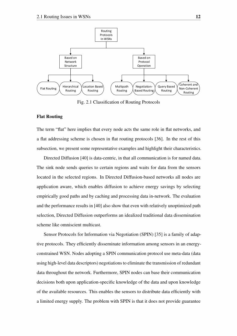
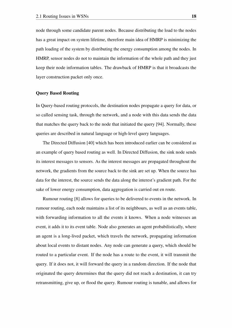
architecture and protocol operation, respectively, as illustrated in Figure 2.1.
2.1.1 Protocols Classification Based on Network Structure
Depending on the underlying network structure, routing protocols can be categorized
into: flat, hierarchical, and location-based routing.
2.1 Routing Issues in WSNs 12
Routing ProtocolsIn WSNs
Based on Network Structure
Based on Protocol
Operation
Flat RoutingHierarchical
RoutingLocation Based
RoutingMultipath Routing
Negotiation-Based Routing
Query Based Routing
Coherent and Non-Coherent
Routing
Fig. 2.1 Classification of Routing Protocols
Flat Routing
The term “flat” here implies that every node acts the same role in flat networks, and
a flat addressing scheme is chosen in flat routing protocols [36]. In the rest of this
subsection, we present some representative examples and highlight their characteristics.
Directed Diffusion [40] is data-centric, in that all communication is for named data.
The sink node sends queries to certain regions and waits for data from the sensors
located in the selected regions. In Directed Diffusion-based networks all nodes are
application aware, which enables diffusion to achieve energy savings by selecting
empirically good paths and by caching and processing data in-network. The evaluation
and the performance results in [40] also show that even with relatively unoptimized path
selection, Directed Diffusion outperforms an idealized traditional data dissemination
scheme like omniscient multicast.
Sensor Protocols for Information via Negotiation (SPIN) [35] is a family of adap-
tive protocols. They efficiently disseminate information among sensors in an energy-
constrained WSN. Nodes adopting a SPIN communication protocol use meta-data (data
using high-level data descriptors) negotiations to eliminate the transmission of redundant
data throughout the network. Furthermore, SPIN nodes can base their communication
decisions both upon application-specific knowledge of the data and upon knowledge
of the available resources. This enables the sensors to distribute data efficiently with
a limited energy supply. The problem with SPIN is that it does not provide guarantee

2.1 Routing Issues in WSNs 13
for data delivery, for instance, when an interested node is very far from the advertised,
then that interested node will not get any data if nodes between these two nodes are not
interested in the data.
Dynamic Source Routing (DSR) [45] adapts quickly to routing changes when hosts
move frequently, yet only requires little or even no overhead during periods in which
hosts move less frequently. This protocol performs well over a variety of environmental
conditions such as host density and movement rates, according to the packet-level
simulation results presented in this paper. However, in large networks where longer
paths prevail, source routing packets cause larger overhead due to the stored path
information.
In AODV [82], each mobile host operates as a specialized router, and routes are
obtained as needed (on-demand) with little or even no reliance on periodic advertise-
ments. AODV is quite suitable for a dynamic self-starting network, as required by
users wishing to utilize ad hoc networks. AODV provides loop-free routes even while
repairing broken links. In addition, this protocol requires no global periodic routing
advertisements, the demand on the overall bandwidth available to the mobile nodes is
significantly less than in those protocols that do necessitate such advertisements. On the
other hand, AODV still inherit most of the advantages of basic distance-vector routing
mechanisms. Nevertheless, since flooding is used for controlling message dissemination
and route maintenance, routing control overhead may grow high [83].
The Topology Dissemination Based on Reverse-Path Forwarding Protocol (TBRPF)
[7] uses the concept of reverse-path forwarding (RPF) to broadcast link-state updates in
the reverse direction along the spanning tree formed by the minimum-hop paths from all
nodes to the source of the update. Within TBRPF, the minimum-hop paths that form the
broadcast trees are computed with the help of topology information received along this
tree. The utilization of minimum-hop trees rather than shortest-path trees (based on link
costs) results in less frequent changes to the broadcast trees (and less communication
cost for maintaining the trees). However, TBRPF requires nodes to maintain routing
tables containing entries for all the nodes in the network, this can bring negative effect

2.1 Routing Issues in WSNs 14
to the scalability of the protocol, especially when user population is large (means large
overhead).
Hierarchical Routing
Hierarchical, or the so called cluster-based routing methods, are with special advantages
in scalability and efficient communication. The term “hierarchical” here means, higher-
energy nodes with higher residual energy are used to process and send the information,
while the ones with lower residual energy can be used to perform the sensing tasks. The
formation of clusters and assigning special tasks to cluster heads can greatly improve the
overall system scalability, lifetime, and energy efficiency. In the rest of this subsection,
we present some representative examples and highlight their characteristics.
Low Energy Adaptive Clustering Hierarchy (LEACH) [34] is a clustering-based
protocol that utilizes randomized rotation of local cluster base stations (cluster-heads)
to evenly distribute the energy load among the sensors in the network. LEACH uses
localized coordination to enable scalability and robustness for dynamic networks, and
incorporates data fusion into the routing protocol to reduce the amount of information
that must be transmitted to the base station. LEACH minimizes global energy usage
by distributing the load to all the nodes at different timing. At different times, each
node has the burden of acquiring data from the nodes in the cluster, fusing the data to
obtain an aggregate signal, and transmitting it to the base station. LEACH is completely
distributed, not requiring any control information from the base station, and the nodes
do not need knowledge of the global network in order to maintain the operation of
LEACH. However, LEACH uses single-hop routing where each node can transmit data
to the cluster-head and the sink directly, hence, it may not be suitable for networks
deployed in large regions.
Power-Efficient Gathering in Sensor Information Systems (PEGASIS) [61] is a near
optimal chain-based protocol that is an enhancement over LEACH. In PEGASIS, each
node communicates only with a nearby neighbour and takes turns transmitting to the
base station, in order to reduce the amount of energy spent per round. PEGASIS outper-

2.1 Routing Issues in WSNs 15
forms LEACH by eliminating the overhead of dynamic cluster formation, minimizing
the distance non leader-nodes must transmit, limiting the number of transmissions and
receives among all nodes, and using only one transmission to the base station per round.
The drawback of PEGASIS protocol is the redundant transmission of the data. This is
due to the fact that PEGASIS does not consider the base station’s location about the
energy of nodes when one of them is selected as the head node.
Hierarchical State Routing (HSR) [79] is a soft state wireless hierarchical routing
protocol. The authors distinguish between the “physical” routing hierarchy (dictated by
geographical relationships between nodes) and “logical” hierarchy of subnets in which
the nodes move as a group HSR keeps track of logical subnet movements using Home
Agent concepts similar to Mobile IP. Compared with flat, table driven routing schemes
(such as DSDV (Highly Dynamic Destination-Sequenced Distance-Vector Routing)
[81]) HSR achieves a much better scalability, at the cost of non-optimal routing and
increased complexity.
Cluster Head Gateway Switch Routing (CGSR) [21] is a multicast protocol inspired
by the Core Based Tree approach (initially developed for the internet). CGSR is robust to
mobility, has low bandwidth overhead and latency, scales well with membership group
size, and can be generalized to other wireless infrastructure (other than hierarchical).
Nevertheless, it is difficult for CGSR to maintain the cluster structure in a mobile
environment.
Location Based Routing
In this type of routing, sensor nodes are addressed according to their locations. The lo-
cation of nodes may be obtained from a satellite if nodes are equipped with GPS (global
positioning system) receiver [116]. Alternatively, nodes can estimate the distance from
neighbours based on incoming signal strengths. Afterwards, the relative coordinates of
neighbouring nodes can be determined by exchanging distance information between
neighbours [9, 10, 97]. In the rest of this subsection, we present some representative
examples and highlight their characteristics.

2.1 Routing Issues in WSNs 16
Geographic Adaptive Fidelity (GAF) [116] saves energy by identifying nodes that
are equivalent from a routing perspective and then shutting down unnecessary nodes,
keeping a constant level of routing fidelity. GAF moderates this policy by using
application-level and system-level information; nodes that source or sink data remain
on and intermediate nodes monitor and balance energy use. GAF focus on turning
the radio off as much as possible. It adapts sleep time based on node location scaling
back node duty cycles (and so reducing routing “fidelity” when many interchangeable
nodes are present. The authors have shown that it performs at least as well as a normal
ad hoc routing protocol for packet loss and route latency while conserving substantial
energy, and allowing network lifetime to increase in proportion to node density. But the
requirement of GPS devices may be difficult for some networks.
SPAN [18] is a location-based and distributed coordination technique that reduces
energy consumption without significantly diminishing the capacity or connectivity of
the network. Within SPAN, nodes make local decisions on whether to sleep, or to join
a forwarding backbone as a coordinator. Each node bases its decision on an estimate
of how many of its neighbours will benefit from it being awake, and the amount of
energy available to it. SPAN provides a randomized algorithm where coordinators rotate
with time, demonstrating how localized node decisions lead to a connected, capacity-
preserving global topology. But on the negative side, existing and new coordinators do
not have to be neighbours, which in fact makes SPAN less energy-efficient because of
the need to maintain the positions of two- or three-hop neighbours.
The Location-Aided Routing (LAR) [54] is an approach to utilize location informa-
tion (for instance, obtained using the global positioning system) to improve performance
of routing protocols for ad hoc networks. By using location information, the LAR pro-
tocols limit the search for a new route to a smaller “request zone” of the ad hoc network.
This leads to in a significant reduction in the number of routing messages. Some algo-
rithms are proposed to determine the so called “request zone”, based on the expected
location of the destination node at the time when route discovery is ongoing. Note that

2.1 Routing Issues in WSNs 17
LAR involves network-wise flooding to obtain location information, which makes the
control overhead increases as the network grows.
2.1.2 Protocols Classification Based on Protocol Operation
Multipath Routing Protocols
In this type of routing, the protocol uses multiple paths instead of a single path, which
has the advantage to enhance network performance. Furthermore, network reliability
can be increased since multipath routing is more resilient to route failures (at the cost of
overhead in maintaining alternative paths).
Label-based Multipath Routing (LMR) [37] is a routing protocol using only local-
ized information. LMR can efficiently find a disjoint or segmented backup path to
provide protection to the working path. LMR utilizes the label information to search
segmented backup path if a disjoint path is not found, reducing overhead and delay.
Furthermore, LMR can take advantage of local multicast, significantly reducing the
routing overhead. However, to find the possible backup paths, LMR consumes extra
overhead, to send label messages, label reinforce messages and backup exploratory
messages.
In [16], the authors formulate the routing problem as to maximize the network
lifetime. This problem formulation has revealed that the minimum total energy (MTE)
routing is not suitable for network-wise optimum utilization of transmission energy. A
shortest cost path routing algorithm is proposed which uses link costs that reflect both
the communication energy consumption rates and the residual energy levels at the two
end nodes. The algorithm is amenable to distributed implementation. It shows that
significant improvement can be made in terms of maximizing the system lifetime, which
can also be interpreted as maximizing the amount of information transfer between the
source and destination nodes with limited energy supply.
The authors of [112] propose a Hierarchy-Based Multipath Routing Protocol
(HMRP) for WSNs. In HMRP, the network will be constructed to layered-network at
first. Based on the layered-network, sensor nodes will have multipath route to sink
2.1 Routing Issues in WSNs 18
node through some candidate parent nodes. Because distributing the load to the nodes
has a great impact on system lifetime, therefore main idea of HMRP is minimizing the
path loading of the system by distributing the energy consumption among the nodes. In
HMRP, sensor nodes do not to maintain the information of the whole path and they just
keep their node information tables. The drawback of HMRP is that it broadcasts the
layer construction packet only once.
Query Based Routing
In Query-based routing protocols, the destination nodes propagate a query for data, or
so called sensing task, through the network, and a node with this data sends the data
that matches the query back to the node that initiated the query [94]. Normally, these
queries are described in natural language or high-level query languages.
The Directed Diffusion [40] which has been introduced earlier can be considered as
an example of query based routing as well. In Directed Diffusion, the sink node sends
its interest messages to sensors. As the interest messages are propagated throughout the
network, the gradients from the source back to the sink are set up. When the source has
data for the interest, the source sends the data along the interest’s gradient path. For the
sake of lower energy consumption, data aggregation is carried out en route.
Rumour routing [8] allows for queries to be delivered to events in the network. In
rumour routing, each node maintains a list of its neighbours, as well as an events table,
with forwarding information to all the events it knows. When a node witnesses an
event, it adds it to its event table. Node also generates an agent probabilistically, where
an agent is a long-lived packet, which travels the network, propagating information
about local events to distant nodes. Any node can generate a query, which should be
routed to a particular event. If the node has a route to the event, it will transmit the
query. If it does not, it will forward the query in a random direction. If the node that
originated the query determines that the query did not reach a destination, it can try
retransmitting, give up, or flood the query. Rumour routing is tunable, and allows for

2.1 Routing Issues in WSNs 19
trade-offs between setup overhead and delivery reliability, but the problem is that it may
broadcast duplicated messages to the same node.
Negotiation-Based Routing
In this type of protocols, meta-data negotiations (high-level data descriptors through
negotiation) are utilized to reduce redundant data transmissions. Communication
decisions can be made based on the resources available to them as well.
The SPIN family protocols [35] mentioned earlier and the protocols in [56] are
examples of negotiation-based routing protocols. The SPIN family of protocols consists
of two basic ideas : first, sensor applications need to communicate with each other about
the data that they already have and the data they still intend to obtain, so as to operate
efficiently and to conserve energy; second, nodes must monitor and adapt to changes in
their own energy resources to maximize the operating lifetime of the network.
QoS-based Routing
In QoS-based routing protocols, the network has to balance between energy consump-
tion and data quality [1, 99]. Specifically, the network has to satisfy certain QoS metrics,
such as delay, energy, bandwidth, and the like, when delivering data to the sink.
In the best-effort routing the main concerns are the throughput and average response
time. QoS routing is usually performed through resource reservation in a connection-
oriented communication that meet the QoS requirements for each individual connection.
While many mechanisms have been proposed for routing QoS constrained real-time
multimedia data in wire based networks, they cannot be directly applied to WSNs due
to the limited resources, such as bandwidth and energy that a sensor node has.
Sequential Assignment Routing (SAR) in [100] is one of the first routing protocols
for WSNs that introduces the concept of QoS in the routing decisions. Routing decision
in SAR depends on the following factors: energy resources, QoS on each path, and
the priority level of each packet. In order to avoid single route failure, a multi-path
approach is used and localized path restoration schemes are adopted. The objective of

2.1 Routing Issues in WSNs 20
SAR algorithm is to minimize the average weighted QoS metric throughout the lifetime
of the network. However, in order to maintain tables and states that store the above
mentioned information at each sensor node, the overhead may be high, especially when
the nodes number is large.
Another QoS routing protocol for WSNs that provides soft real-time end-to-end
guarantees is SPEED [32], which is designed to avoid congestion when the network
is congested. The routing module in SPEED is called Stateless Geographic Non-
Deterministic forwarding (SNFG) and works with four other modules at the network
layer. Compared to DSR and AODV which are mentioned earlier, SPEED performs
better in terms of end-to-end delay and miss ratio. Furthermore, the total transmission
energy and control packet overhead are less because of the simplicity of the routing
algorithm. Nevertheless, the performance of of SPEED is not very good when the
network is heavily congested.
Coherent and Non-coherent Based Routing
In operation of WSNs, data processing is a major component. The sensor nodes
cooperate with each other in processing the data within the network. The routing
mechanism which initiates the data processing module is proposed in [100]. This
mechanism is divided into two categories: coherent and non-coherent data-processing
based routing. For non-coherent based routing [46], the raw data is processed by sensor
nodes locally before it is sent to other nodes (aggregators) for further processing. In
coherent based routing, only minimum processing (such as time stamping and duplicate
suppression) is done for raw data before it is sent to aggregators.
In [11, 100], Single Winner Algorithm (SWE) and Multiple Winner Algorithm
(MWE) are proposed for non-coherent and coherent processing, respectively.
In SWE, a single aggregator node is elected for complex processing. This node is
selected based on the energy reserves and computational capability of that node. At
the end of the SWE process, a minimum-hop spanning tree will completely cover the
network.

2.2 Energy Efficient Routing Protocols 21
MWE is a simple extension of SWE. When all nodes are sources and send their data
to the central aggregator node, a large amount of energy will be consumed. In order
to lower the energy cost, limit the number of sources that can send data to the central
aggregator node is a possible solution. Instead of keeping a record of only the best
candidate node, each node will keep a record of up to n nodes of those candidates. At
the end of the MWE process, each sensor in the network holds a set of minimum-energy
paths to each source node. After that, SWE is utilized to determine the node that yields
the minimum energy consumption.
2.2 Energy Efficient Routing Protocols
The most straightforward thinking of improving energy efficiency of WSNs is to
design energy efficient sensors. Work was started in academic institutions, but a
number of enterprises have joined the team in recent years, including companies such
as Crossbow, Dust Networks, Ember Corporation, Sensoria and Wordsens. These
commercial efforts make the sensor devices ready for real deployment in various WSN
applications, together with a serious of tools for sensor programming and maintenance
[76].
In parallel to the progress in sensor hardware, some efforts have been made to
improve the energy efficiency of the routing protocols themselves. For example, the
distributed position-based routing method described in [90] attempts to minimize the
energy consumed for routing data packets, but the drawback is that location information
is required. Given any number of randomly deployed nodes over an area, a simple local
optimization scheme executed at each node guarantees strong connectivity of the entire
network and attains the global minimum energy solution for stationary networks. Due
to its localized nature, this protocol is self-reconfiguring.
Another approach of minimum cost message delivery studied in [119] is called
Scalable Solution to Minimum-Cost Forwarding (SSMCF). This approach seeks the
minimum cost path from any given source to a specific sink in sensor networks. This ap-

2.3 Energy Harvesting Aware Routing Protocols 22
proach may not be suitable for some WSN applications because the sink (or destination
node) is assumed to be fixed.
Efficient Minimum-Cost Bandwidth-Constrained Routing (EMCBCR) [15] is de-
signed to select the routes and the corresponding power levels for the sake of maximizing
the time until batteries of the nodes drain-out. EMCBCR is local and amenable to
distributed implementation. If there is a single power level, the problem is reduced
to a maximum flow problem with node capacities and the algorithms converge to the
optimal solution. If there are multiple power levels then the achievable lifetime is close
to the optimal most of the time. EMCBCR is a simple, scalable and efficient solution for
minimum cost routing in WSNs. In fact the term “minimum cost” refers to maximum
network lifetime, achieved by choosing the route with maximum energy reserve which
is not exactly the same as a route with minimum energy cost.
2.3 Energy Harvesting Aware Routing Protocols
Another research direction to improve energy efficiency is to consider renewable energy
from an external energy source. Renewable energy can be harvested from the surround-
ing environment by various means such as solar, wind, thermal, or motion [13], that
is, energy harvesting which has been introduced in Section 1.3.1. Solar power is well
suited to WSNs because not only sunlight is easy to access but also solar panels can be
made small enough to be mounted on wireless sensor nodes.
A notable routing algorithm that is energy harvesting aware is the Distributed Energy
Harvesting Aware Routing Algorithm (DEHAR) [42], which defines a new metric of
“energy distance” (including energy harvesting) for selecting the best route. By this
metric, DEHAR aims to find the route with minimum total energy distance rather than
spatial distance. DEHAR calculates the shortest energy distance by using a method
such as Directed Diffusion, a flooding mechanism incurring extra routing overhead.
Opportunistic Routing algorithm with Adaptive Harvesting-aware Duty Cycling
(OR-AHaD) proposed in [6] is designed with energy management capabilities that
consider variations in the availability of the environmental energy. OR-AHaD can

2.4 Conventional Types of Attack on WSNs 23
Attacker
Sensor 1 Sensor 2
Packets:
1, 2, 3, 4, 5,
...
Packets:
4, 5, 6, ...
Fig. 2.2 Selective forwarding attack
adjust the duty cycle of each node adaptively in order to exploit the available energy
resources efficiently in comparison to other opportunistic routing protocols. However,
geographical information is required, which may not be well suited to some applications.
2.4 Conventional Types of Attack on WSNs
Security challenges in WSNs are similar to those in mobile ad hoc networks identified
in [101, 123]. As being military applications, the network faces the risk of attacks from
enemies to interfere with operations, such as selective forwarding, wormhole attacks,
sinkhole attacks, and Sybil attacks [2, 49]. Nodes may become compromised which
could be very difficult to detect. It is commonly assumed that compromised nodes may
exhibit suspicious behaviour, which can be monitored and factored into a reputation
system that calculates a reputation for every node and adapts route selections to avoid
nodes with low reputations. Moreover, suspected nodes are prevented from participating
in the routing protocol.
Below are examples of some conventional attacks that are the main threats to routing
in WSNs.
2.4.1 Selective Forwarding Attack (Grey Hole Attack)
As illustrated in Figure 2.2, compromised nodes may refuse to forward certain messages
and just simply drop them, so that they can never reach the original destination. This

2.4 Conventional Types of Attack on WSNs 24
Attacker
Sensor 1 Sensor 2
Sensor 3 Sensor 4
Packets Packets
Packets Packets
Fig. 2.3 Sinkhole attack
Attacker
Sensor 1
Sensor 2
Sensor 3
Sensor 4
Fig. 2.4 Sybil attack
threat can make things even worse if a malicious node is explicitly included on the route
[117].
2.4.2 Sinkhole Attack
As shown in Figure 2.3, a compromised node tries to attract all surrounding nodes to
establish routes through itself. If the sinkhole attack is successful, then the network is
also vulnerable to other attacks, such as eavesdropping or selective forwarding [71].
2.4.3 Sybil Attack
As illustrated in Figure 2.4 [117], the malicious node creates multiple fake identities to
other neighbouring nodes in the network [70]. This Sybil attack is especially harmful

2.4 Conventional Types of Attack on WSNs 25
to geographic and multipath routing protocols, since the malicious node can appear in
multiple positions [49].
In addition, the authors of [69, 70] have discussed more routing attacks that can
threat WSNs, e.g. fairness attack, sleep attack [85], and wormhole attack [51].
2.4.4 Existing Attack Countermeasures: Detection and Elimina-
tion of Malicious Behaviours
To deal with Grey hole attack, the Forwarding Assessment Based Detection (FADE)
[63] scheme is proposed to mitigate collaborative grey hole attacks. Specifically, FADE
detects sophisticated attacks by means of forwarding assessments aided by two-hop
acknowledgement monitoring. Moreover, FADE can coexist with contemporary link
security techniques. The optimal detection threshold, that minimizes the sum of false
positive rate and false negative rate of FADE, is analysed while considering the network
dynamics due to degraded channel quality or medium access collisions.
For sink hole attack, [73] present an algorithm for detecting the intruder. This
algorithm first makes a list of suspected nodes, and then effectively identifies the
intruder in the list through a network flow graph. The algorithm is also robust to deal
with cooperative malicious nodes that attempt to hide the real intruder.
As to Sybil Attack, [122] investigates Sybil attacks and defence schemes in Internet
of Things (IoT). The authors first define three types of Sybil attacks according to the
Sybil attacker’s capabilities, then present some Sybil defence schemes, including Social
Graph-Based Sybil Detection (SGSD), Behaviour Classification-Based Sybil Detection
(BCSD), and mobile Sybil detection with the comprehensive comparisons.
In [86] the authors develop a system-theoretic approach to security that provides a
complete protocol suite with provable guarantees. This approach is based on a model
capturing the essential features of an ad hoc wireless network that has been infiltrated
with hostile nodes. The protocol suite caters to the complete life cycle, all the way
from the birth of nodes, through all phases of ad hoc network formation, leading to an
optimized network carrying data reliably. This approach has a distinguished feature: it

2.4 Conventional Types of Attack on WSNs 26
supersedes much of the previous work that deals with several types of attacks (usually
one approach can only deal with a specific type of attack) including wormhole, rushing,
partial deafness, routing loops, routing black holes, routing grey holes, and network
partition attacks.
2.4.5 Existing Attack Countermeasures: Efforts Made on Routing
Solutions
Some existing routing protocols such as TinySec [48], SPINs [84], TinyPK [113], and
TinyECC [62] attempt to eliminate unauthorized behaviour of malicious sensor nodes
with the help of encryption or authentication on data packets. However, these solutions
may be difficult for WSNs. For instance, data encryption is applicable for mobile
ad hoc networks but generally not practical for WSNs because sensors have limited
data processing capability and energy storage. Therefore, in addition to cryptographic
solutions, routing algorithms that employ notions of trust and reputation have been
proposed.
A trust-based reactive multipath routing protocol, Ad hoc On-Demand Trusted-path
Distance Vector (AOTDV) [59], is an extension of the AODV routing protocol and
the Ad hoc On-demand Multipath Distance Vector (AOMDV) [67] routing protocol.
This protocol is able to discover multiple loop-free paths as candidates in one route
discovery. These paths are evaluated by two aspects: hop counts and trust values.
This two-dimensional evaluation provides a flexible and feasible approach to choose
the shortest path from the candidates that meet the requirements of data packets for
dependability or trust.
LTB-AODV [66], is light-weight in the sense that the intrusion detection system
(IDS) used for estimating the trust that one node has for another, consumes limited
computational resource. Moreover, it uses only local information thereby ensuring
scalability. Our light-weight IDS takes care of two kinds of attacks, namely, the black
hole attack and the grey hole attack. Whereas the proposed approach can be incorporated

2.5 Routing Protocols Including Energy Efficiency and Security 27
in any routing protocol. Note that the authors have used AODV as the base routing
protocol.
The above two approaches passively observe forwarded data traffic and then calcu-
late the risk level of different routes in terms of “trust values”, the routing algorithm
then chooses the most trusted route. But there are some drawbacks: first, reputation
system used in AOTDV or LTB-AODV watches for a single specific behaviour only;
furthermore, they solely focus on security with no special attention given to energy
efficiency concerns. Therefore, new routing solutions that can monitor multiple node
behaviours and make comprehensive judgements on node status, while giving enough
attention to the crucial energy efficiency are worth studying.
2.5 Routing Protocols Including Energy Efficiency and
Security
There are a few papers starting to consider security and energy efficiency at the same
time.
For instance, Ferng and Rachmarini [28] proposed a secure routing protocol for
WSNs considering energy efficiency. With the location and energy-aware characteristics
for routing, the protocol gives a better delivery rate, energy balancing, and routing effi-
ciency. In addition, the proposed security mechanism ensures the data authenticity and
confidentiality in the data delivery. But it has a disadvantage requiring information about
node locations to improve energy efficiency. Furthermore, it depends on encryption
which can be a heavy computation cost for sensor nodes.
Lightweight Secure LEACH (LS-LEACH) [4] aims to provide a secure and energy
efficient routing protocol. Cryptographic authentication algorithm is integrated to
assure data integrity, authenticity and availability. Furthermore, LS-LEACH shows its
improvement over LEACH protocol that makes it secure and more energy efficient (by
reducing the overhead from added security measures).

2.6 Security Concerns of Energy Depletion Attacks on WSNs 28
The above schemes generate extra overhead, thus the grantee of security with
reduced energy cost could be a research of interest.
2.6 Security Concerns of Energy Depletion Attacks on
WSNs
Since sensors deployed in WSNs have limited computation and energy resources, they
are vulnerable to resource depletion attacks, such as Denial of Service (DoS) attack and
the forced authentication attacks [33].
The power draining attack is a sub-category of resource depletion attack, given that
battery is considered as the resource of interest. Rather than disabling the immediate
availability, a power draining attack is trying to deplete the network’s power over a long
time horizon. Vampire attacks, an instance of the power draining attack, target routing
protocols used in WSNs even those designed to be secure [110]. Vampire attacks are
not protocol-specific. Instead, they exploit the general properties of routing protocols.
Even worse, they use protocol-compliant messages, which makes themselves difficult
to be detected and prevented.
Some simple attempts similar to Vampire attacks have been made, such as the power
draining or resource exhaustion attacks described in [78, 102]. Rather than generating
tremendous data to paralyse the network, Vampire attacks tend to inflict harm on the
network little by little. Since Vampire attacks comply with the existing routing protocols,
and data deliveries will be accomplished at the end (but just cost more resources than
usual), these features make them even more difficult to be detected.
Existing routing protocols usually do not employ authentication in controlling
messages, which give opportunity to adversaries. Thus adversaries are free to alter the
information in control messages. Vampire attackers can take advantage of the above
mentioned features and organize attacks in the form of [110]:

2.6 Security Concerns of Energy Depletion Attacks on WSNs 29
strength of their attack by selecting destinations designed tomaximize energy usage.
Per-node energy usage under both attacks is shown inFig. 2. As expected, the carousel attack causes excessiveenergy usage for a few nodes, since only nodes along ashorter path are affected. In contrast, the stretch attackshows more uniform energy consumption for all nodes inthe network, since it lengthens the route, causing morenodes to process the packet. While both attacks significantlynetwork-wide energy usage, individual nodes are alsonoticeably affected, with some losing almost 10 percent oftheir total energy reserve per message. Fig. 3a diagrams theenergy usage when node 0 sends a single packet to node 19in an example network topology with only honest nodes.Black arrows denote the path of the packet.
Carousel attack. In this attack, an adversary sends a packetwith a route composed as a series of loops, such that the samenode appears in the route many times. This strategy can beused to increase the route length beyond the number ofnodes in the network, only limited by the number ofallowed entries in the source route.2 An example of thistype of route is in Fig. 1a. In Fig. 3b, malicious node 0 carriesout a carousel attack, sending a single message to node 19(which does not have to be malicious). Note the drasticincrease in energy usage along the original path.3 Assumingthe adversary limits the transmission rate to avoid saturat-ing the network, the theoretical limit of this attack is anenergy usage increase factor of Oð�Þ, where � is themaximum route length.
Overall energy consumption increases by up to a factorof 3.96 per message. On average, a randomly locatedcarousel attacker in our example topology can increasenetwork energy consumption by a factor of 1:48� 0:99. Thereason for this large standard deviation is that the attackdoes not always increase energy usage—the length of theadversarial path is a multiple of the honest path, which is inturn, affected by the position of the adversary in relation tothe destination, so the adversary’s position is important tothe success of this attack.
Stretch attack. Another attack in the same vein is thestretch attack, where a malicious node constructs artificially longsource routes, causing packets to traverse a larger thanoptimal number of nodes. An honest source would select the route Source! F ! E ! Sink, affecting four nodes includ-
ing itself, but the malicious node selects a longer route,affecting all nodes in the network. These routes cause nodesthat do not lie along the honest route to consume energy by
322 IEEE TRANSACTIONS ON MOBILE COMPUTING, VOL. 12, NO. 2, FEBRUARY 2013
Fig. 2. Node energy distribution under various attack scenarios. Thenetwork is composed of 30 nodes and a single randomly positionedVampire. Results shown are based on a single packet sent by theattacker.
Fig. 3. Energy map of the network in terms of fraction of energyconsumed per node. Black arrows show the packet path through thenetwork. Each dotted line represents an “energy equivalence zone,”similar to an area of equal elevation on a topological chart. Each line ismarked with the energy loss by a node as a fraction of total originalcharge.
2. The ns-2 DSR implementation arbitrarily limits the route length to 16.3. Energy usage is greatest at node 10 likely due to its distance from its
nearest neighbors.
Fig. 2.5 Example: route loop attack (carousel attack)
strength of their attack by selecting destinations designed tomaximize energy usage.
Per-node energy usage under both attacks is shown inFig. 2. As expected, the carousel attack causes excessiveenergy usage for a few nodes, since only nodes along ashorter path are affected. In contrast, the stretch attackshows more uniform energy consumption for all nodes inthe network, since it lengthens the route, causing morenodes to process the packet. While both attacks significantlynetwork-wide energy usage, individual nodes are alsonoticeably affected, with some losing almost 10 percent oftheir total energy reserve per message. Fig. 3a diagrams theenergy usage when node 0 sends a single packet to node 19in an example network topology with only honest nodes.Black arrows denote the path of the packet.
Carousel attack. In this attack, an adversary sends a packetwith a route composed as a series of loops, such that the samenode appears in the route many times. This strategy can beused to increase the route length beyond the number ofnodes in the network, only limited by the number ofallowed entries in the source route.2 An example of thistype of route is in Fig. 1a. In Fig. 3b, malicious node 0 carriesout a carousel attack, sending a single message to node 19(which does not have to be malicious). Note the drasticincrease in energy usage along the original path.3 Assumingthe adversary limits the transmission rate to avoid saturat-ing the network, the theoretical limit of this attack is anenergy usage increase factor of Oð�Þ, where � is themaximum route length.
Overall energy consumption increases by up to a factorof 3.96 per message. On average, a randomly locatedcarousel attacker in our example topology can increasenetwork energy consumption by a factor of 1:48� 0:99. Thereason for this large standard deviation is that the attackdoes not always increase energy usage—the length of theadversarial path is a multiple of the honest path, which is inturn, affected by the position of the adversary in relation tothe destination, so the adversary’s position is important tothe success of this attack.
Stretch attack. Another attack in the same vein is thestretch attack, where a malicious node constructs artificially longsource routes, causing packets to traverse a larger thanoptimal number of nodes. An honest source would select the route Source! F ! E ! Sink, affecting four nodes includ-
ing itself, but the malicious node selects a longer route,affecting all nodes in the network. These routes cause nodesthat do not lie along the honest route to consume energy by
322 IEEE TRANSACTIONS ON MOBILE COMPUTING, VOL. 12, NO. 2, FEBRUARY 2013
Fig. 2. Node energy distribution under various attack scenarios. Thenetwork is composed of 30 nodes and a single randomly positionedVampire. Results shown are based on a single packet sent by theattacker.
Fig. 3. Energy map of the network in terms of fraction of energyconsumed per node. Black arrows show the packet path through thenetwork. Each dotted line represents an “energy equivalence zone,”similar to an area of equal elevation on a topological chart. Each line ismarked with the energy loss by a node as a fraction of total originalcharge.
2. The ns-2 DSR implementation arbitrarily limits the route length to 16.3. Energy usage is greatest at node 10 likely due to its distance from its
nearest neighbors.
Fig. 2.6 Example: stretch attack
• Route loop attack (carousel attack): as shown in Figure 2.5, in this attack pattern,
an adversary purposely introduces routing loops and makes the same data packet
travel repeatedly through the same group of nodes.
• Stretch Attack: as illustrated in Figure 2.6, in this attack pattern, an adversary
tries to establish unnecessarily long routes, potentially passing through as many as
possible nodes in the network. We call this the stretch attack because it increases

2.7 Summary 30
average route length, forcing packets to be received and forwarded by a number
of nodes that are initially not supposed to participate.
To the best of our knowledge, there has been very little discussion on the prevention
against the Vampire attacks. The existing proposed solution, such as PLGPa [110], a
modified version of PLGP (clean-slate secure sensor network routing protocol) [78],
highly rely on cryptographic methods, which can incur extra computation and transmis-
sion cost. Considering the limited computing capability and energy storage of wireless
sensors, better (meaning more energy efficient and requiring less hardware) mitigation
scheme is worth investigating.
2.7 Summary
In this chapter, previous works on WSN routing protocols with various concerns have
been reviewed. Furthermore, the security challenges for WSNs, together with the
existing countermeasures and potential opportunities were presented as well.

Chapter 3
AODV-EHA: Energy Harvesting
Aware Routing Protocol
3.1 Introduction
As addressed in Section 2.1, one limitation of traditional routing attempts for WSNs
is that they just try to cope with either of two features, namely, WSN’s ad hoc nature
and the utilization of energy harvesting technology in WSNs. Therefore, in this chapter,
we propose the AODV-EHA that not only inherits the advantage of existing AODV on
dealing with WSN’s ad hoc nature, but also make use of the energy harvesting capability
of the sensor nodes in the network.
The rest of this chapter is organized as follows. Section 3.2 summarizes background
knowledge and theoretical analysis of AODV-EHA and its competitors. Section 3.3
provides simulation results that illustrating the advantage of the proposed routing
protocol. The summary and further issues are in Section 3.4.

3.2 Comparison of AODV-EHA and Competitors 32
3.2 Comparison of AODV-EHA and Competitors
3.2.1 Overview of Original AODV Routing Protocol
As stated in [80], the network that adopts AODV is silent until a connection is requested.
After that the sender (or source) node that needs a connection broadcasts a Route
Request (RREQ) for connection. Other nodes in the network forward this message, and
record the node that they heard it from, creating temporary routes back to the sender
node. When a node receives such a message and already has a route to the desired
receiver (or destination) node, it sends a Route Reply (RREP) backwards through a
temporary route to the requesting node. The sender node then adopts the route with
least hops through other nodes.
Eventually, the original AODV protocol attempts to figure out the route with least
communication hops from any source node to the destination node. In other words,
suppose the total number of possible routes in between is Nr and along any i-th route
(i is an integer and 1 ≤ i ≤ Nr) there are Ji nodes, if the k-th route is the optimal one
determined by AODV, then it satisfies Jk=min[J1,J2, ...,JNr ].
3.2.2 Overview of DEHAR
As mentioned in Section 3.1, the basic idea of DEHAR is to introduce a new concept of
“energy distance”. The energy distance between a certain sender node and its receiver
node can be considered as a weighted spatial distance that is related to the current energy
status (how much energy could be harvested from ambient) of the sender. Assume along
any i-th route, the total energy distance D(i) is defined as
D(i) = D(i,1)+D(i,2)+ ...+D(i,Ji−1) (3.1)
Suppose m is an integer and 1≤ m≤ (Ji−1), thus D(i,m) is the energy distance
from node m to m+ 1 and D(i,m) = d(i,m)+ f [α(i,m)], where d(i,m) is the spatial
distance between node m and m+ 1 on the i-th route, α(i,m) is the energy could be

3.2 Comparison of AODV-EHA and Competitors 33
dist
ance
pena
lty
harvested energy 0 at bt ct 1
θ
γ a = 0.25b = 0.75c = 0.90α = 50β = 5
Fig. 4. Example of relation between energy availability and local distancepenalty.
To add energy awareness the available energy e : E in anode must be measured, where E ∧
= [0; 1] (normalised withrespect to the energy storage capacity C). Then it is convertedinto a distance penalty f : E → D where D ∧
= R≥0. For anynode, this distance penalty is a local distance penalty, for thatnode.
To be meaningful, f should be monotonically decreasing,where the ideal situation is that f approaches zero whenthere is plenty of energy, i.e. f(e) → 0, when e → 1,and f approaches infinity when there is lack of energy, i.e.f(e) → ∞, when e → 0. In a concrete WSN these idealsituations must be approximated.
All nodes are informed about their neighbours’ distancesto sink (including penalties) and choose the least expensive /cheapest neighbour for routing. A distance including penaltiesis now defined as energy distance. Hence the term shortestdistance is excluding any penalties while the shortest energydistance includes penalties.
An example of a function for transforming the measuredenergy availability e : E to the local distance penalty fpl
(e) :D is shown in (6). This is further exemplified with Fig. 4.
fpl(e) =
0 , 1 ≥ e > cβ e−c
b−c , c ≥ e > b
(α− β) e−ba−b + β , b ≥ e ≥ a
α , a > e ≥ 0
(6)
The values a, b and c are different thresholds of energyavailability. c determines the upper bound for sensitivity. a isthe lower bound for energy availability. b describes the point ofchange between different sensitivities of variations in energyavailability together with the penalty amplitude β. α describesthe maximum penalty.
A limited energy availability is now applied to the examplenetwork (the shaded area) in Fig. 5. This results in localdistance penalties to the nodes Ng and Nf . In this particularexample there is a local minimum distance to sink at nodeNe. This is an undesirable situation as Ne has no neighbourto whom it would be (on the basis of the energy distance withlocal penalties) natural to send packages to.
The distributed distance penalties are designed to solve theproblem with local minima which the local distance penaltiescan create. Every node communicates changes in their energyinformation to its immediate neighbours. Each time a nodereceives an update from a neighbour, it checks if it is in a localminimum. If so, it increase its distributed distance penalty to
dist
anced
Nod
e
local distance penalties dlshortest distance ds
Nx Na Nb Nc Nd Ne Nf Ng Nx
sink
sink
Nx
Na
Nb
Nc
NdNe
Nf
Ng
Fig. 5. The example network in Fig. 3 now displays an area with low energyavailability (shaded area) in the right graph. This results in local distancepenalties in the left graph.
dist
anced
Nod
e
distributed distance penalties ddlocal distance penalties dlshortest distance ds
Nx Na Nb Nc Nd Ne Nf Ng Nx
sink
sink
Nx
Na
Nb
Nc
NdNe
Nf
Ng
Fig. 6. The example network from Fig. 3 and Fig. 5 is now completed withthe distributed penalties. Now all nodes have a sustainable route to sink.
solve the problem and reports this to its neighbours throughan update.
This process also works the other way around, where a nodechecks whether its distributed distance penalty is unreasonablehigh and lowers it appropriately. In the example network, thedistributed distance penalty is now added (see Fig. 6). We shallnow present an algorithm which is based on these ideas.
C. Algorithm
Each node runs the same set of algorithms to managethe local and distributed distance penalties. These algorithmsmanage a set of variables which constitutes the state of a node.It also manages a copy of the state of all neighbouring nodes.Furthermore it is assumed that each node uses the same localdistance penalty function fpl
: E → D.Consider a node N (see Fig. 7) having kn neighbours N ={N1, N2, . . . , Nkn}. The node N has four state variables
ds :D Shortest distance to sink.dl :D Local penalty.dd :D Distributed penalty.r : {1, . . . , kn} Index of neighbour to route to.
Furthermore, for each neighbour Ni of N , there are two statevariables:
dsi :D The shortest distance to sink of Ni.dpi :D The total penalty of Ni.
Based on that information the neighbour Nr, with the shortestenergy distance to sink, is found.
Note that the local and distributed penalties are mergedinto one total penalty before it is distributed, hence onlythe total penalty of a neighbour is known to a node. Thestates ds and dsi are managed by an algorithm for findingthe shortest structural distance and is therefore not changedby this algorithm.
Fig. 3.1 Relation between energy availability and distance penalty
harvested and used for data transmission at m-th node that is defined over [0,1] (nor-
malized with respect to the energy required for transmission). The function f [α(i,m)]
can be considered as “distance penalty” (more harvested energy refers to less distance
penalty and vice-versa) and defined as:
f [α(i,m)] =
0 , 1≥ αim > ct
θα(i,m)−ct
bt−ct, ct ≥ αim > bt
(γ−θ)α(i,m)−btat−bt
+θ , bt ≥ α(i,m)≥ at
γ , at > α(i,m)≥ 0
(3.2)
where at , bt and ct are different thresholds of energy that can be harvested for data
transmission. As already defined in [42], ct determines the upper bound for sensitivity,
at is the lower bound for energy availability, and bt describes the point of change
between different sensitivities of variations in energy availability. Further, θ and γ are
the penalty amplitude and maximum penalty, respectively. The author provides a chart
showing an example of relation between energy availability and distance penalty in
Figure 3.1 (in this example at = 0.25, bt = 0.75, ct = 0.9, γ = 50, θ = 5).
As illustrated in Figure 3.1, in order to add energy awareness, α(i,m) is converted
into a distance penalty f [α(i,m)]. f [α(i,m)] is monotonically decreasing, where the
ideal situation is that f [α(i,m)] approaches zero when there is plenty of energy, i.e.

3.2 Comparison of AODV-EHA and Competitors 34
RFC 3561 AODV Routing July 2003
RREQ ID A sequence number uniquely identifying theparticular RREQ when taken in conjunction with theoriginating node’s IP address.
Destination IP AddressThe IP address of the destination for which a routeis desired.
Destination Sequence NumberThe latest sequence number received in the pastby the originator for any route towards thedestination.
Originator IP AddressThe IP address of the node which originated theRoute Request.
Originator Sequence NumberThe current sequence number to be used in the routeentry pointing towards the originator of the routerequest.
5.2. Route Reply (RREP) Message Format
0 1 2 3 0 1 2 3 4 5 6 7 8 9 0 1 2 3 4 5 6 7 8 9 0 1 2 3 4 5 6 7 8 9 0 1 +-+-+-+-+-+-+-+-+-+-+-+-+-+-+-+-+-+-+-+-+-+-+-+-+-+-+-+-+-+-+-+-+ | Type |R|A| Reserved |Prefix Sz| Hop Count | +-+-+-+-+-+-+-+-+-+-+-+-+-+-+-+-+-+-+-+-+-+-+-+-+-+-+-+-+-+-+-+-+ | Destination IP address | +-+-+-+-+-+-+-+-+-+-+-+-+-+-+-+-+-+-+-+-+-+-+-+-+-+-+-+-+-+-+-+-+ | Destination Sequence Number | +-+-+-+-+-+-+-+-+-+-+-+-+-+-+-+-+-+-+-+-+-+-+-+-+-+-+-+-+-+-+-+-+ | Originator IP address | +-+-+-+-+-+-+-+-+-+-+-+-+-+-+-+-+-+-+-+-+-+-+-+-+-+-+-+-+-+-+-+-+ | Lifetime | +-+-+-+-+-+-+-+-+-+-+-+-+-+-+-+-+-+-+-+-+-+-+-+-+-+-+-+-+-+-+-+-+
The format of the Route Reply message is illustrated above, and contains the following fields:
Type 2
R Repair flag; used for multicast.
A Acknowledgment required; see sections 5.4 and 6.7.
Reserved Sent as 0; ignored on reception.
Perkins, et. al. Experimental [Page 8]
Fig. 3.2 RREQ message format in original AODV [80]
f [α(i,m)]→ 0, when α(i,m)→ 1, and f [α(i,m)] approaches maximum penalty γ
when there is lack of energy, i.e. f [α(i,m)]→ γ , when α(i,m)→ 0.
The optimal route (denoted by the k-th route) determined by DEHAR satisfies the
condition D(k) = min[D(1),D(2), ...,D(Nr)]. Note that after all the spatial distance are
encoded to “energy distance”, DEHAR calculates the shortest energy distance by using
existing method such as Directed Diffusion.
3.2.3 New AODV-based Routing Approach: AODV-EHA
As mentioned in Section 3.1, the AODV-EHA utilizes the advantages of original AODV
together with the promising energy harvesting simultaneously: not only adapted to the
ever changing network topology (the entire network does not need to be known by the
routing algorithm in advance), but also achieving energy efficiency for a longer network
lifetime. All these features are achieved by making full use of the existing mechanism
of AODV without extra complexity and routing overhead.
Suppose that a process at source node wants to send a packet to destination node,
the AODV-EHA algorithm maintains an energy vector table at each node in the network,
keyed by destination, giving information about that destination, including the neighbour
to which to send packets to reach the destination. First, source node looks in its table.
If the source node does not find an entry for destination, it has to discover a route to
destination node. This property of discovering routes only when they are needed is
what makes this algorithm “on-demand”.
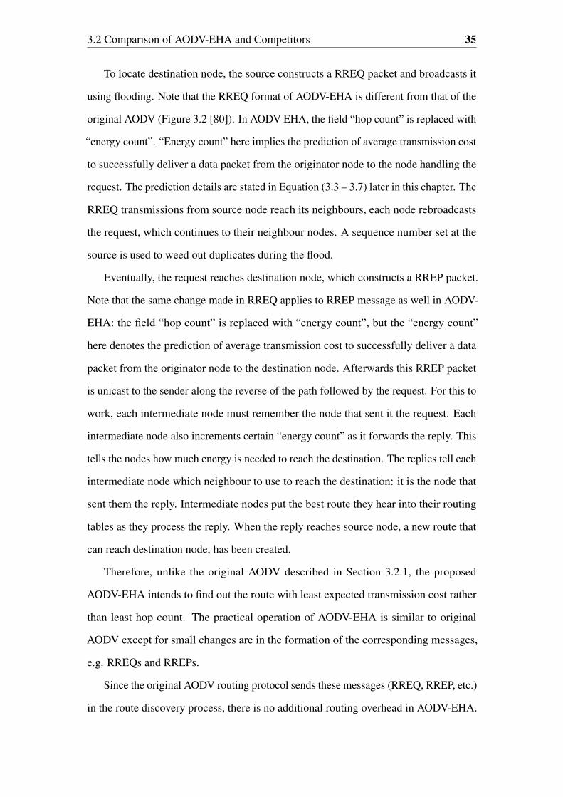
3.2 Comparison of AODV-EHA and Competitors 35
To locate destination node, the source constructs a RREQ packet and broadcasts it
using flooding. Note that the RREQ format of AODV-EHA is different from that of the
original AODV (Figure 3.2 [80]). In AODV-EHA, the field “hop count” is replaced with
“energy count”. “Energy count” here implies the prediction of average transmission cost
to successfully deliver a data packet from the originator node to the node handling the
request. The prediction details are stated in Equation (3.3 – 3.7) later in this chapter. The
RREQ transmissions from source node reach its neighbours, each node rebroadcasts
the request, which continues to their neighbour nodes. A sequence number set at the
source is used to weed out duplicates during the flood.
Eventually, the request reaches destination node, which constructs a RREP packet.
Note that the same change made in RREQ applies to RREP message as well in AODV-
EHA: the field “hop count” is replaced with “energy count”, but the “energy count”
here denotes the prediction of average transmission cost to successfully deliver a data
packet from the originator node to the destination node. Afterwards this RREP packet
is unicast to the sender along the reverse of the path followed by the request. For this to
work, each intermediate node must remember the node that sent it the request. Each
intermediate node also increments certain “energy count” as it forwards the reply. This
tells the nodes how much energy is needed to reach the destination. The replies tell each
intermediate node which neighbour to use to reach the destination: it is the node that
sent them the reply. Intermediate nodes put the best route they hear into their routing
tables as they process the reply. When the reply reaches source node, a new route that
can reach destination node, has been created.
Therefore, unlike the original AODV described in Section 3.2.1, the proposed
AODV-EHA intends to find out the route with least expected transmission cost rather
than least hop count. The practical operation of AODV-EHA is similar to original
AODV except for small changes are in the formation of the corresponding messages,
e.g. RREQs and RREPs.
Since the original AODV routing protocol sends these messages (RREQ, RREP, etc.)
in the route discovery process, there is no additional routing overhead in AODV-EHA.
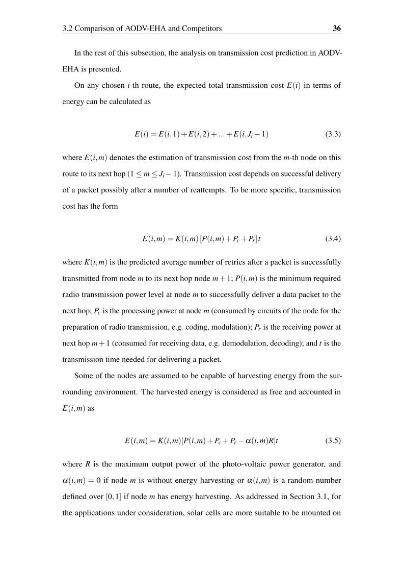
3.2 Comparison of AODV-EHA and Competitors 36
In the rest of this subsection, the analysis on transmission cost prediction in AODV-
EHA is presented.
On any chosen i-th route, the expected total transmission cost E(i) in terms of
energy can be calculated as
E(i) = E(i,1)+E(i,2)+ ...+E(i,Ji−1) (3.3)
where E(i,m) denotes the estimation of transmission cost from the m-th node on this
route to its next hop (1≤m≤ Ji−1). Transmission cost depends on successful delivery
of a packet possibly after a number of reattempts. To be more specific, transmission
cost has the form
E(i,m) = K(i,m) [P(i,m)+Pc +Pr] t (3.4)
where K(i,m) is the predicted average number of retries after a packet is successfully
transmitted from node m to its next hop node m+1; P(i,m) is the minimum required
radio transmission power level at node m to successfully deliver a data packet to the
next hop; Pc is the processing power at node m (consumed by circuits of the node for the
preparation of radio transmission, e.g. coding, modulation); Pr is the receiving power at
next hop m+1 (consumed for receiving data, e.g. demodulation, decoding); and t is the
transmission time needed for delivering a packet.
Some of the nodes are assumed to be capable of harvesting energy from the sur-
rounding environment. The harvested energy is considered as free and accounted in
E(i,m) as
E(i,m) = K(i,m)[P(i,m)+Pc +Pr−α(i,m)R]t (3.5)
where R is the maximum output power of the photo-voltaic power generator, and
α(i,m) = 0 if node m is without energy harvesting or α(i,m) is a random number
defined over [0,1] if node m has energy harvesting. As addressed in Section 3.1, for
the applications under consideration, solar cells are more suitable to be mounted on

3.3 Performance Evaluation 37
sensor nodes considering the size (e.g. wind driven generator is too bulky) or energy
source accessibility (e.g. motion power is hard to access since nodes operate in severe
environment where human activity is rare).
For these nodes, α(i,m) = R′/R where R
′is the active power level of the photo-
voltaic power generator. For a photo-voltaic power generator [47], its active power is
assumed to follow a β−distribution given by the following probability density function:
F(R′) =
Γ(psh +qsh)
Γ(psh)Γ(qsh)
(R′
R
)psh−1(1− R
′
R
)qsh−1
(3.6)
where psh and qsh are the shape parameters of the distribution, and Γ is the Gamma
function. Beta distributions are fit to the past record of sunlight data using the algorithm
that minimizes the K–S statistic [23], and its shape parameters psh and qsh depend on
the specific geographic location where sunlight data are recorded. This assumption is
also based on the past recorded sunlight data and statistical correlation analysis of solar
radiance and consumer load.
From [53], in order to successfully transmit a packet from node m to its next hop
node m+1, the expected average number of retries K(i,m) can be calculated as
K(i,m) =1
1−Pout(i,m)(3.7)
where Pout(i,m) is the probability of the packet not been delivered (or outage probabil-
ity) from node m to node m+1 on any attempt. Based on the previous work in [95],
Pout(i,m) can be expressed as a function in P(i,m).
Eventually the optimal route (denoted by the k-th route) determined by proposed
AODV-EHA satisfies that E(k) = min [E(1),E(2), ...,E(Nr)].
3.3 Performance Evaluation
In this section, the performance of original AODV, AODV-EHA and the DEHAR
protocols are analysed under MATLAB platform. The word “performance” here implies:

3.3 Performance Evaluation 38
• Average transmission cost between any two arbitrary nodes within the network
after a data packet is successfully delivered.
• Average hop count of the route (may be determined by any routing protocol)
where the data packet travelled through between those two arbitrary nodes.
Then the performance of these three routing approaches are compared and the relation-
ship between them is revealed.
3.3.1 Route Discovery in Simulator
The simulator utilizes Dijkstra algorithm [24] to determine the optimal route under
different routing protocols. Dijkstra algorithm was originally designed for finding the
shortest paths between nodes in a graph, and the “shortest” here implies shortest distance.
If we replace the factor “distance” for other metrics, e.g. “hop count” (for AODV),
“energy distance” (for DEHAR), and “energy count” (for AODV-EHA), Dijkstra can be
utilized to find the optimal route as if AODV or DEHAR or AODV-EHA is adopted. Of
course, the practical operation of these 3 protocols in real world are different, but the
eventual results (determined optimal routes) are the same.
Some simple examples of the optimal routes determined by AODV, DEHAR and
AODV-EHA using the simulator are illustrated in Figure 3.3 – 3.5: 50 nodes are
randomly distributed in the fixed simulation area (500 m×500 m), normal nodes are
denoted by black dot with node number, nodes with energy harvesting capability are
denoted by green dot with node number. Suppose the objective is to find a route from
node 41 to node 31. The estimated energy consumption to deliver a single packet along
41→ 31 determined by AODV (with least hop count) is approximately 0.000612 Joule;
meanwhile that of DEHAR and AODV-EHA along 41→ 31 (longer route but least
transmission cost) are approximately 0.000608 Joule and 0.000491 Joule, respectively.
A few simple examples are far from enough, thus the simulations using Monte-
Carlo approach are performed: certain number of nodes are randomly distributed in the
fixed simulation area, pick any one of them and evaluate the performance under the 3

3.3 Performance Evaluation 39
0 100 200 300 400 500
50
100
150
200
250
300
350
400
450
AODV routing in WSN
X−axis in meter
Y−
axis
in m
eter
1
2
3
4
5
6
7
8
9
10
11
12
13
14
15
16
17
18
19
20
21
22
23
24
25
2627
28
29
30
31
32
33
34
35
36
37
38
39
40
41
42
43
44
45
46
4748
49
50
Fig. 3.3 A simple example: route Determined by AODV
0 100 200 300 400 500
50
100
150
200
250
300
350
400
450
DEHAR routing in WSN
X−axis in meter
Y−
axis
in m
eter
1
2
3
4
5
6
7
8
9
10
11
12
13
14
15
16
17
18
19
20
21
22
23
24
25
2627
28
29
30
31
32
33
34
35
36
37
38
39
40
41
42
43
44
45
46
4748
49
50
Fig. 3.4 A simple example: route determined by DEHAR
different routing protocols when delivering a data packet back to a specific destination
node. Repeat this process for a large enough number of times, then evaluate average
performance of the three routing protocols.

3.3 Performance Evaluation 40
0 100 200 300 400 500
50
100
150
200
250
300
350
400
450
AODV−EHA routing in WSN
X−axis in meter
Y−
axis
in m
eter
1
2
3
4
5
6
7
8
9
10
11
12
13
14
15
16
17
18
19
20
21
22
23
24
25
2627
28
29
30
31
32
33
34
35
36
37
38
39
40
41
42
43
44
45
46
4748
49
50
Fig. 3.5 A simple example: route determined by AODV-EHA
3.3.2 Simulation Setup
IEEE 802.15.4 is a leading standard that is widely used in WSNs, this standard focuses
on low data-rate, and low-power ubiquitous communication among devices [39, 114].
According to the specification mentioned in [39], lower data rates of 20 and 40 kbps
were initially defined, with maximum 250 kbps rate being supported in the current
revision [115]. Lower data rates bring not only less power consumption, but also
lower manufacturing cost and technological simplicity, without sacrificing flexibility
Table 3.1 Simulation setup
Parameters DescriptionsSimulation Area 500 m × 500 m
Node Radio Range 250 mTraffic Type CBRPacket Size 127 bytesData Rate 20 kbps
Threshold β 10Processing Power Level Pc 10−4 WReceiving Power Level Pr 5×10⁻⁵ W
Outage Requirement P∗out(i,m) 10−4
3.3 Performance Evaluation 41
or generality. The medium access control (MAC) enables the transmission of MAC
frames through the use of the physical channel. Note that the IEEE 802.15 standard
does not utilize 802.1d or 802.1q, in other words, standard Ethernet frames cannot
be exchanged. The physical frame-format is specified in [39], and it is tailored to the
fact that most IEEE 802.15.4 PHYs only support frames of up to 127 bytes (since the
frame is generally composed of frame header, payload data from upper layer and frame
footer, thus this limitation can affect some settings in upper layer, such as packet size in
network layer).
As mentioned above, if we choose IEEE 802.15.4 for the physical and data link layer,
which is suitable for the nominated WSN applications in this dissertation (low data
rate but very long battery life), the settings of data rate and packet size in simulations
are confined by this choice. Therefore, in all our simulations we assume the traffic
type is constant bit rate (CBR) with a data rate of 20 Kbps and the packet size is 127
bytes, as illustrated in 3.1. Note that lower data rate means longer transmitting time,
lower transmission power level and longer processing time when a node is sending
data packets. On the other hand, larger packet size means longer transmission time for
delivering a packet. Therefore, the choice of data rate and packet size can affect the
calculation of expected transmission cost along a specific route (details can be found in
Section 3.2.3). As a result, when we are simulating route discoveries in AODV-EHA,
the metric “energy count” (see Section 3.3.1 for details) used in the simulator can be
affected by the settings of data rate and packet size, and this may influence the final
result of optimal route under AODV-EHA. In addition, the transmission cost evaluations
(later addressed in Section 3.3.3) can be influenced by these settings as well.
Other parameters also can be found in Table 3.1: for each single hop transmission,
Pc denotes the data processing power consumed by a transmitting node, receiving node
consumes Pr power units to receive the data. The values of the parameters Pr , Pc and the
communication range of each node are assumed the same for all nodes in the network
and are specified by the manufacturer. Outage requirement P∗out(i,m) is defined as the
maximum tolerated probability that the received SNR at receiving node falls below a

3.3 Performance Evaluation 42
certain threshold β . If the received SNR is higher than the threshold β , the receiver is
assumed to be able to decode the received message with negligible probability of error.
If an outage occurs, the packet is considered lost. The SNR threshold β is determined
according to the application and the transmitter/ receiver structure.
3.3.3 Simulation Results
The simulations use Monte-Carlo approach considering two typical simulation scenarios:
Scenario 1: stationary destination node.
This scenario can be considered as the application of environment surveillance. The
engineer just stays at a fixed observation point in the region where the WSN is deployed,
and collects data from the nodes. The number of nodes varies from 10 to 90.
10 20 30 40 50 60 70 80 90
Number of nodes
0.5
1
1.5
2
2.5
3
3.5
4
4.5
Ave
rage
end
to e
nd tr
ansm
issi
on c
ost (
Joul
e)
10-3
Original AODVDEHARAODV-EHA
Fig. 3.6 Average transmission cost versus the number of nodes
Figure 3.6 compares the average end-to-end transmission cost of original AODV,
DEHAR and AODV-EHA, after a data packet is successfully delivered. Figure 3.7 – 3.8
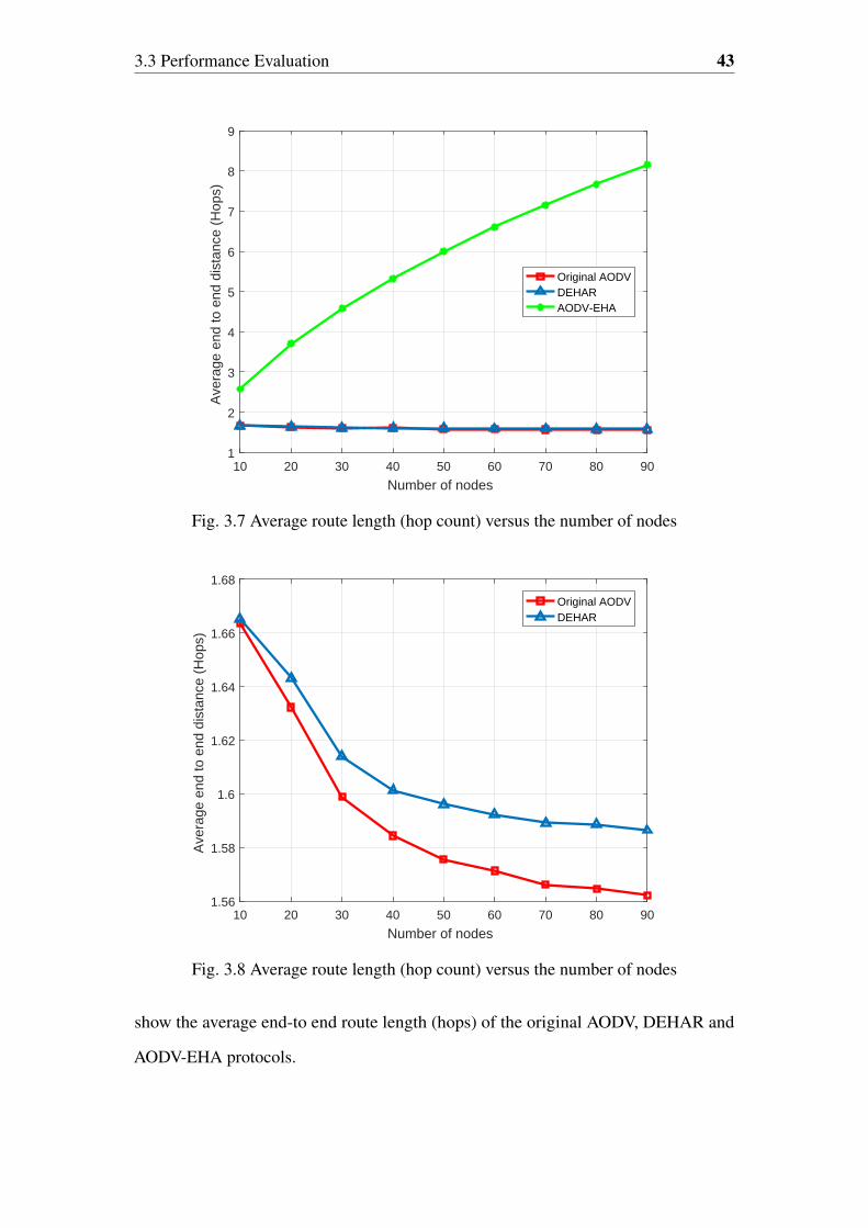
3.3 Performance Evaluation 43
10 20 30 40 50 60 70 80 90
Number of nodes
1
2
3
4
5
6
7
8
9
Ave
rage
end
to e
nd d
ista
nce
(Hop
s)
Original AODVDEHARAODV-EHA
Fig. 3.7 Average route length (hop count) versus the number of nodes
10 20 30 40 50 60 70 80 90
Number of nodes
1.56
1.58
1.6
1.62
1.64
1.66
1.68
Ave
rage
end
to e
nd d
ista
nce
(Hop
s)
Original AODVDEHAR
Fig. 3.8 Average route length (hop count) versus the number of nodes
show the average end-to end route length (hops) of the original AODV, DEHAR and
AODV-EHA protocols.
3.3 Performance Evaluation 44
From Figure 3.6, we can conclude that as the number of nodes increase, both the
average transmission cost of AODV-EHA and DEHAR decrease gradually, and AODV-
EHA overcomes DEHAR in any case in terms of energy saving. By contrast, the same
records of original AODV fluctuate along with the nodes number increases, and showing
an apparent descending tendency, but shows more cost compared to that of DEHAR and
AODV-EHA in all instances. The fluctuation of energy cost using AODV is because
the AODV is seeking for the route with least hops, but less hops does not always bring
less energy cost in wireless transmissions, as been discussed before [95]. Note that
lower transmission cost means less energy consumption for all the nodes involved in
transmission, that is, given a same battery capacity, the nodes are expected to operate a
longer time and send more data. Therefore the network lifetime can be prolonged as
well. For example, when the nodes number is 50, the nodes in the network adopting
AODV-EHA are expected to send approximately 44.42% more data packets at most
(compare to the adoption of DEHAR).
On the other hand, under AODV-EHA, the route length is increasingly high as the
number of nodes in the area goes up, while that of original AODV and DEHAR are
slightly reduced, as can be seen from 3.7 (the results of original AODV and DEHAR are
further presented in Figure 3.8 that otherwise their difference cannot be seen clearly). A
longer route length may lead to longer end-to-end delay, but normally it should not be
a problem in this scenario, e.g. meteorological observation frequency is normally at
minute level [57].
Scenario 2: destination node with mobility.
This scenario can be considered as the application of enemy detection in the bat-
tlefield. An engineer (or data collecting device) can be assigned to any position in the
area where WSN is deployed, not tied a fixed place as in scenario 1. In the same way as
in scenario 1, the Monte-Carlo approach is adopted except the only difference is the
position of data collecting point is random instead of stationary. The number of nodes
varies from 10 to 90.

3.3 Performance Evaluation 45
10 20 30 40 50 60 70 80 90
Number of nodes
0.5
1
1.5
2
2.5
3
3.5
4
4.5
Ave
rage
end
to e
nd tr
ansm
issi
on c
ost (
Joul
e)
10-3
Original AODVDEHARAODV-EHA
Fig. 3.9 Average transmission cost versus the number of nodes
Figure 3.9 compares the average end-to-end transmission cost of original AODV,
AODV-EHA and the DEHAR, after a data packet is successfully delivered. Figure 3.11-
3.10 show the average end-to end route length (hops) of the original AODV, DEHAR,
and AODV-EHA protocols.
From Figure 3.9, we can conclude that as the number of nodes increase, the average
transmission cost of AODV-EHA and DEHAR decrease gradually, and AODV-EHA
overcomes DEHAR in any case in terms of energy saving. By contrast, the same records
of original AODV fluctuate along with the nodes number increases, and showing an
unapparent descending tendency, but has more cost compared to that of DEHAR and
AODV-EHA in all instances.
On the other hand, under AODV-EHA, the route length is increasingly high as
the nodes number in the area goes up, as can be seen in Figure 3.10 (the results of
original AODV and DEHAR are further presented in Figure 3.11 that otherwise their
difference cannot be seen clearly). Longer route length may lead to longer end-to-end
delay, which could negatively affect time sensitive applications such as the one in this
scenario. Thus before making the decision, the exact delay-tolerance level, energy

3.3 Performance Evaluation 46
10 20 30 40 50 60 70 80 90
Number of nodes
1
2
3
4
5
6
7
8
9
Ave
rage
end
to e
nd d
ista
nce
(Hop
s)
Original AODVDEHARAODV-EHA
Fig. 3.10 Average route length (hop count) versus the number of nodes
10 20 30 40 50 60 70 80 90
Number of nodes
1.56
1.58
1.6
1.62
1.64
1.66
1.68
Ave
rage
end
to e
nd d
ista
nce
(Hop
s)
Original AODVDEHAR
Fig. 3.11 Average route length (hop count) versus the number of nodes
consumption requirement, nodes distribution density, etc., for practical situation should
be carefully evaluated, and see which routing protocol will be the best trade-off between
those factors concerning.

3.4 Summary 47
3.4 Summary
In this chapter, we introduced the AODV-EHA routing protocol for environmental, mili-
tary, or commercial WSN applications. In these applications, nodes are usually deployed
without careful pre-planning and are not static after initial deployment. Meanwhile
nodes are energy sensitive since they usually work in severe environment and battery
replacement are usually not possible. AODV-EHA not only inherits the advantage of
existing AODV on dealing with WSN’s ad hoc nature, but also makes use of the energy
harvesting capability of the sensor nodes in the network. Consequently, AODV-EHA
achieved both energy efficiency and capability of handling network topology change.
Through simulations, we evaluated the performance of original AODV, AODV-EHA
and the DEHAR routing protocols. Although AODV-EHA usually finds the longest
routing paths, it has the smallest transmission overhead along the determined routes.
Chapter 4
ETARP: An Energy Efficient
Trust-Aware Routing Protocol
4.1 Introduction
While routing protocols have been proposed for either energy efficiency or security,
as been discussed in Chapter 2, the new routing protocol proposed in this chapter
balances these two concerns simultaneously by means of utility theory. To the best of
our knowledge, this is an original approach for WSN routing protocols. An essential
component of the routing protocol is the method to estimate energy consumption for
packet forwarding. Another essential element is a Bayesian network to judge the
probability of each node being compromised (which serves as a measure of trust or
reputation).
The rest of this chapter is organized as follows. Section 4.2 gives the background
knowledge on utility theory together with a few related work. Section 4.3 presents the
central concepts in the new ETARP. The methods used to estimate energy consumption
and risk of node compromise are explained. Performance evaluation in terms of
simulation results is presented in Section 4.4. Section 4.5 summarize this chapter.
4.2 Essentials to Utility Theory 49
4.2 Essentials to Utility Theory
4.2.1 General Concept
Utility is a quite general concept known from microeconomics. Many classical books
on economics have addressed the field of utility theory exhaustively, such as [65] by
Mankiw and [108, 109] by Varian. In the rest of this subsection, some parts of the utility
theory that are closely related to this dissertation are given.
Economists in Victoria days used utility as a numeric measure of the term “satisfac-
tion” or “happiness”, normally the utility was sensitive to the price and quantity of the
goods. Given this idea, it was natural to think of consumers making choices so as to
maximize their utility, that is, to make themselves as happy as possible.
The drawback of this idea is that how to exactly measure the utility is not really
described by these economists, then some consequent questions arise: is one person’s
utility the same as another person’s? What is the meaning to say that an extra bottle of
coke-cola would give somebody twice as much utility as an extra cup of apple juice?
Does the concept of utility have any independent meaning other than its being what
people maximize?
Due to these conceptual problems, modern economists have abandoned the old-
fashioned view of utility as being a measure of happiness. Instead, the theory of
consumer behaviour has been reformulated entirely in terms of “consumer preferences”,
and utility is seen only as a way to describe preferences. Economists gradually began to
recognize that all that mattered about utility as far as choice behaviour was concerned
was whether one commodity had a higher utility than another—how much higher did
not really matter. Originally, preferences were defined in terms of utility: to say a
commodity x was preferred to a commodity y meant that the x-commodity had a higher
utility than the y-commodity. But now we tend to think of things the other way around.
The preferences of the consumer are the fundamental description useful for analysing
choice, and utility is simply a way of describing preferences.

4.2 Essentials to Utility Theory 50
The only property of a utility assignment that is important is how it orders the
commodities. The value of the utility is only important insofar as it ranks the different
consumption commodities; the size of the utility difference between any two consump-
tion commodities does not matter. Because of this emphasis on ordering commodities,
this kind of utility is referred to as ordinal utility.
A utility function is a way of assigning a value to every possible consumption
commodity such that more-preferred commodities get assigned larger numbers than
less-preferred commodities. That is, a commodity x is preferred to a commodity y if
and only if the utility of x is larger than the utility of y: in symbols, x≻ y if and only if
u(x)> u(y).
Since only the ranking of the commodities matters, there can be no unique way to
assign utilities to commodities. If we can find one way to assign utility numbers to
commodities, we can find an infinite number of ways to do it, as long as they satisfy:
x≻ y if and only if u(x)> u(y). If u(x) represents a way to assign utility value to the
commodity x, then multiplying u(x) by 2 (or any other positive number) is just as good
a way to assign utilities.
Multiplication by 2 is an example of a monotonic transformation. A monotonic
transformation is a way of transforming one set of numbers into another set of numbers
in a way that preserves the order of the numbers. If f (u) is any monotonic transformation
of a utility function that represents some particular preferences, then f [u(x)] is also
a utility function that represents those same preferences. Examples of monotonic
transformations are multiplication by a positive number (e.g. f (u) = 6u), adding
any number (e.g., f (u) = u+ 8), raising u to an odd power (e.g. f (u) = u5), and so
on. This above discussion can be summarized by stating the following principle: a
monotonic transformation of a utility function is a utility function that represents the
same preferences as the original utility function.

4.2 Essentials to Utility Theory 51
4.2.2 Utility Theory Applied in Network Research
In network research, utility usually refers to the satisfaction the network user derives
from obtaining the service provided by the network. Initiated by the work of [50] on
network utility maximization (NUM), utility theory has been extensively employed for
certain directions in network research. Previous researches conclude that utility theory
is one of the most popular choices applied on resource allocation [22, 105] and network
selection [111] in wireless networks. In rest of this subsection we highlight some of the
utility-based network researches.
In [19], a centralised, utility-based resource allocation scheme for mixed traffic in
wireless networks is proposed. In this paper, the unified utility function for users with
different traffics is studied first. After that, the optimization model for the resource
allocation is established based on the unified utility function. A heuristic algorithm
based on the solution of the model is proposed in the mixed traffic scenario after
analysing the optimization model. The algorithm which has lower complexity than the
existing work can automatically guarantee the QoS requirement for the real-time traffic
and make a trade-off between throughput and fairness for users with best effort traffic
due to the unified utility function.
The authors in [74] focus on utility models in the context of access network selection.
In this paper, the utility theory is adapted and consolidated to define an appropriate
decision mechanism in the frame of the access network selection. Subsequently, they
propose single-criterion and multi-criteria utility forms to best capture the user satisfac-
tion and sensitivity facing up to multiple access network characteristics (e.g. cost, QoS,
and network load).
In [12], utility theory and bankruptcy game are applied in joint bandwidth allocation
for heterogeneous integrated wireless networks, by combining throughput and cost utili-
ties for network selection and resource allocation. The proposed bandwidth allocation
scheme consists of two successive stages, namely, service bandwidth allocation and
user bandwidth allocation. Note that this paper assumes that monetary costs on the user
imposed by different access networks are non-identical.

4.3 ETARP Routing 52
Enemy Intrusion DetectionOn Battlefield
Normal Sensor Node
Sensor with
Energy Harvesting
Data collecting point with mobility
Compromised Node
Source Node
Enemy IntrusionDetected
Other Choices of RouteOptimal Route determined by ETARP
Node’s status determined by Bayesian
Network
Fig. 4.1 Example of WSN application scenario
4.3 ETARP Routing
This section describes the ETARP routing protocol designed for the WSN applications
mentioned in Chapter 1. The routing protocol aims to simultaneously consider energy
efficiency and security to avoid routes that are inefficient and risky. In order to simplify
the description, we assume for the moment a “normal” condition absent of attacks in
the network. In this case, ETARP works to discover and select the most energy efficient
routes. In the next section, attacks on the network will be taken into account to show
how ETARP factors trustworthiness of nodes into the route selection. Because energy
efficiency and security are two different problems, ETARP takes a novel approach of
factoring both using the notion of expected utility.
A basic example to demonstrate the idea of ETARP is shown in Figure 4.1. After the
enemy appears in the WSN covered region, their activity can be detected by a nearby
sensor node (e.g. acoustic or seismic sensor) which will send warning information back
to the data collection point. Usually this process cannot be accomplished in a single
hop transmission. ETARP aims to find the most energy efficient multi-hop route while
simultaneously avoiding any (perceived) compromised nodes. The status of nodes is

4.3 ETARP Routing 53
Type R A Reserved Prefix Sz Hop CountDestination IP address
Destination Sequence NumberOriginator IP address
Lifetime
Fig. 4.2 RREQ message format in original AODV
estimated by a Bayesian network that collects data about observed node behaviors and
calculates the probability that each node is compromised or not.
4.3.1 Energy Efficiency Routing in Absence of Attacks
For the moment, attacks on the network are ignored in order to present how ETARP
operates to discover and select energy efficient routes. Previous studies have found that
the ad hoc nature of the network dictates an on-demand routing protocol such as AODV.
However, AODV aims to minimize hop count without consideration of energy costs.
ETARP is based on AODV but adds awareness of transmission energy costs.
Route discovery by ETARP operates similarly to AODV except for a different
format of the routing messages: RREQs, RREPs, and so on. The format of the RREQ
message in the original AODV is shown in Figure 4.2 [80].
The same change applies to the RREP message as well. The field “hop count” in the
original AODV RREP message is replaced with “energy count” in the ETARP RREP
message.
Since ETARP uses the same basic messages (e.g. RREQ and RREP) as AODV, it
does not incur more overhead compared to the original AODV. The next question is
how to define energy consumption for the new “energy count” message field.
Similar to the definitions from Equation (3.3 – 3.7), on any chosen i-th route
spanning a total number of Ji nodes, the expected total transmission cost E(i) in terms
of energy can be calculated as
E(i) = E(i,1)+E(i,2)+ ...+E(i,Ji−1) (4.1)

4.3 ETARP Routing 54
where E(i,m) is the estimated transmission cost from the m-th node on this route to its
next hop (1≤ m≤ Ji−1). In specific, E(i,m) has the form
E(i,m) = K(i,m) [P(i,m)+Pc +Pr] t (4.2)
For nodes that are assumed to be capable of harvesting solar energy, E(i,m) is
rewritten as
E(i,m) = Kim[P(i,m)+Pc +Pr−α(i,m)R]t (4.3)
After ETARP discovers a number of possible routes, say with energy costs {E(1),E(2),
. . ., E(Nr)}, it selects the route with the minimum energy cost.
4.3.2 Energy Efficient and Secure Routing in Presence of Attacks
The previous section dealt with the simple case of energy efficient routing assuming
normal conditions without attacks on the network. The possibility of attacks adds
complications because nodes can become compromised and interfere with packet
forwarding.
Our approach to add security awareness into ETARP relies on the concept of
“expected utility” from utility theory. Either transmission energy or risk of untrusted
nodes will diminish the expected utility of a route. ETARP seeks routes with high
expected utility which will be both energy efficient and trusted.
Definition of Utility in WSN
In WSNs, each node can be considered as a “customer”, multiple choices of paths within
the network that leads to destination node in data transmission represent the various
“commodities” in the “market”. And different route will bring different “consumer
preferences”, in other words, different utility, to a node that is scheduled to transmit
data. Rather than “price” and “quantity”, the utility or preference designated for a route
is related to both energy cost and security level (trustworthiness).

4.3 ETARP Routing 55
Consider a specific route consisting of J nodes (J−1 hops). Considering only energy
on any specific hop, say the m-th hop, the utility function is inversely proportional to
the predicted transmission cost on this hop. Less energy consumption means a longer
lifetime that is more “preferable” for the sensor nodes and therefore a higher utility.
Then the utility function of the m-th hop, denoted by u(
1Em
), satisfies
u(
1Em
)∝
1Em
(4.4)
where Em (how to determine Em can be found in Section 4.3.1) is the estimated trans-
mission cost from the m-th node on this route to its next hop (1≤ m≤ J−1) .
The transmission on each hop takes place successively over time, starting from
the source node and ending at the destination node. The utility of all these hops are
imperfect substitutes to each other, meaning that some reduction in utility of the m-
th hop might be compensated for, to some extent, by the addition of another hop’s
utility and vice versa. But this is not always the case, e.g. if the m-th hop is a dead
link, no matter how good condition the other hops are, this route is considered to be
useless with zero total utility. Due to this imperfect substitutes property, the utility
function of a specific route belongs to the Cobb-Douglas type with standard form
of Uroute = uc11 uc2
2 uc33 . . ., where uc1
1 ,uc22 ,uc3
3 , . . . denote the utility generated from first,
second, third, and so on until the last (J−1)th hop on a route, respectively. That is, the
utility of a route is the product of utilities on all the J−1 hops [108]. On the other hand,
wireless sensors deployed in a specific network typically belong to the same type with
identical technical specifications, thus the sender nodes at each hop can be considered
to be identical and use the same utility function to describe their “preference”. In this
case, the multiple J−1 hops transmission on this route can be considered as equivalent
to a node repeating a single hop transmission J−1 times. Then the total utility on this
route can be written as
Uroute
(1
Em
)=
J−1
∏m=1
u(
1Em
)=
J−1
∏m=1
(1
Em
)cro
(4.5)

4.3 ETARP Routing 56
where cro is a positive constant indicating the “preference” level of each hop, which is
related to the sensitivity to energy cost. Note that the numerator in the last part in (4.5)
corresponds to the energy consumption factor on each hop, which is already explained
in (4.3) of Section 4.3.1. As mentioned earlier in Section 4.2.1, u(
1Em
)=(
1Em
)crois
just one of the many ways to assign utility, there is an infinite number of ways to do
it. Any functions, as long as they satisfy: u(
1Em1
)> u
(1
Em2
)(m1,m2 are integers and
m1,m2 ∈ m) if and only if 1Em1
> 1Em2
, can be utilized to assign utility—including but
not limited to logarithmic function (e.g. u(
1Em
)= log2
1Em
) and exponential function
(e.g. u(
1Em
)= 2
1Em ). Some of the convex functions (e.g. u
(1
Em
)= e
1Em ) and concave
functions (e.g. u(
1Em
)= log 1
Em) also can be valid choices as long as they are monotone
increasing in their domains and can satisfy the above mentioned condition.
Calculation of Expected Utility
At each hop, there is a certain risk that the next node is compromised. In other words,
there is never certainty about the status of any node (malicious or not). Given this
uncertainty, we introduce the weighted average of utilities gained from all the possible
results (malicious node or not) as the “expected utility” u′(
1Em
):
u′(
1Em
)=(Hm +(1−Hm)Qm)u
(1
Em
)+(1−Hm)(1−Qm)0
=(Hm +(1−Hm)Qm)u(
1Em
) (4.6)
where Hm is the probability that the destination node is safe (not compromised); and
Qm is the possibility that the destination node is compromised but pretends to behave
like normal node (a so-called “grey hole”). How to determine the probability Hm is
explained in Section 4.3.3. If the node is safe or pretending to be normal, the utility of
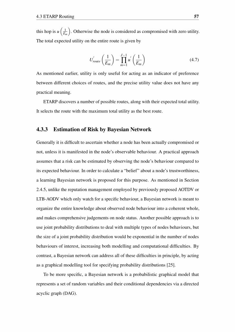
4.3 ETARP Routing 57
this hop is u(
1Em
). Otherwise the node is considered as compromised with zero utility.
The total expected utility on the entire route is given by
U′route
(1
Em
)=
J−1
∏m=1
u′(
1Em
)(4.7)
As mentioned earlier, utility is only useful for acting as an indicator of preference
between different choices of routes, and the precise utility value does not have any
practical meaning.
ETARP discovers a number of possible routes, along with their expected total utility.
It selects the route with the maximum total utility as the best route.
4.3.3 Estimation of Risk by Bayesian Network
Generally it is difficult to ascertain whether a node has been actually compromised or
not, unless it is manifested in the node’s observable behaviour. A practical approach
assumes that a risk can be estimated by observing the node’s behaviour compared to
its expected behaviour. In order to calculate a “belief” about a node’s trustworthiness,
a learning Bayesian network is proposed for this purpose. As mentioned in Section
2.4.5, unlike the reputation management employed by previously proposed AOTDV or
LTB-AODV which only watch for a specific behaviour, a Bayesian network is meant to
organize the entire knowledge about observed node behaviour into a coherent whole,
and makes comprehensive judgements on node status. Another possible approach is to
use joint probability distributions to deal with multiple types of nodes behaviours, but
the size of a joint probability distribution would be exponential in the number of nodes
behaviours of interest, increasing both modelling and computational difficulties. By
contrast, a Bayesian network can address all of these difficulties in principle, by acting
as a graphical modelling tool for specifying probability distributions [25].
To be more specific, a Bayesian network is a probabilistic graphical model that
represents a set of random variables and their conditional dependencies via a directed
acyclic graph (DAG).
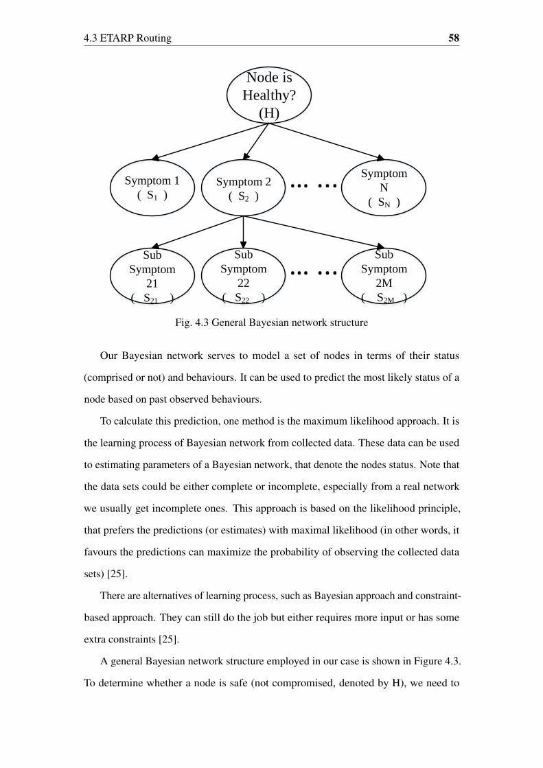
4.3 ETARP Routing 58
Node is
Healthy?
(H)
Symptom 1
( S1 )
Symptom
N
( SN )
Symptom 2
( S2 )… ...
Sub
Symptom
21
( S21 )
Sub
Symptom
22
( S22 )
… ...Sub
Symptom
2M
( S2M )
Fig. 4.3 General Bayesian network structure
Our Bayesian network serves to model a set of nodes in terms of their status
(comprised or not) and behaviours. It can be used to predict the most likely status of a
node based on past observed behaviours.
To calculate this prediction, one method is the maximum likelihood approach. It is
the learning process of Bayesian network from collected data. These data can be used
to estimating parameters of a Bayesian network, that denote the nodes status. Note that
the data sets could be either complete or incomplete, especially from a real network
we usually get incomplete ones. This approach is based on the likelihood principle,
that prefers the predictions (or estimates) with maximal likelihood (in other words, it
favours the predictions can maximize the probability of observing the collected data
sets) [25].
There are alternatives of learning process, such as Bayesian approach and constraint-
based approach. They can still do the job but either requires more input or has some
extra constraints [25].
A general Bayesian network structure employed in our case is shown in Figure 4.3.
To determine whether a node is safe (not compromised, denoted by H), we need to

4.3 ETARP Routing 59
Node is Not
Compromised?
(H)
Node Used to
Drop Packets?
(D)
Node
Participated in
Routing
Before?
(P)
Fig. 4.4 A Bayesian network example
observe the node’s symptoms; some symptoms may require further observation of their
sub-symptoms.
Consider a basic practical example shown in Figure 4.4. The purpose is to determine
a node’s “health” status (node is compromised or not), denoted by variable H. Two
symptoms are considered: the first is “node used to drop packets” (denoted by variable
D). Note that it is normal for a node to drop a packet sometimes for a valid reason, e.g.
bad link quality, but the term “drop packet” here implies that the number of dropped
packets is unusually large. Also, “node participated in routing before or not” (denoted
by variable P), can help to identify attacks including selective forwarding, sink hole,
black and grey hole. These variables are binary, represented by T (true) or F (false)
for variable H, D and P. Nodes in this DAG represent the aforementioned propositional
variables. Edges in the graph represent “direct causal influences” among these variables,
e.g. the node participated in routing before (P) is a direct cause of node not being
compromised (H). All these causal influences are presented by conditional probabilities,
an example shown in the last two sub-tables of Table 4.2 (which is also an example of
initial estimates to be explained later). Given this causal structure, one would expect
the dynamics of changing belief to satisfy some properties. For example, if we get a
record that the sensor node dropped a packet, our belief that the node participated in
routing before would probably decrease.

4.3 ETARP Routing 60
Table 4.1 Incomplete data sets D
D H D Pobservation1 ? F Tobservation2 ? T Fobservation3 ? T T
In practical cases, the recorded node symptoms (referred to as data sets) may be
incomplete due to some reason, e.g. a node being compromised or not cannot be
directly observed (in fact the purpose of creating Bayesian network is to determine it).
Table 4.1 shows an example of incomplete data sets D with 3 different recorded data
cases: observation1, observation2 and observation3. A data case is a record of a set
of symptoms shown by a node, in other word, a record with certain combination of
instantiation (h, d, p), in which the status parameters (h,d, p)= (T,T,T ) denote that this
node has not been compromised, used to drop packet and participated in routing before,
respectively, and (h,d, p) = (F,F,F) denote that this node has been compromised, not
used to drop packet and not participated in routing before, respectively. The symbol “?”
represents the missing values of variables.
The goal is to calculate the expected empirical distribution of nodes status H based on
the incomplete data set. Some initial estimates are assumed as shown in Table 4.2, where
F(h = T ) denotes the probability of a node is not compromised (F(h = F) represents
the probability of contrary status), and F(d = T |h = T ) denotes the probability of
a node used to drop packet given that it is not compromised (by such analogy, the
denotations of all the other combinations of F(d|h) and F(p|h) can be obtained). The
initial estimates are based on common sense: a comprised node is more likely to drop
data packets and not participate in previous routing. By contrast, a healthy node (not
compromised) is more likely to participate in routing, but may still drop data packets
for some reason, e.g. data transmission error.
Then a local search method, called expectation maximization (EM), is employed.
That is, we first completes the data set (we have only got incomplete one as shown
in table 4.1 so far), inducing an empirical distribution, and then uses it to estimate
parameters. To illustrate the process of completing a data set, consider again the data

4.3 ETARP Routing 61
Table 4.2 Initial estimates
H F(h)T 0.8F 0.2
H D F(d|h)T T 0.1T F 0.9F T 0.8F F 0.2
H P F(p|h)T T 0.5T F 0.5F T 0.25F F 0.75
Table 4.3 Completed data sets
H D P FD(.)T T T To be determinedT T F To be determinedT F T To be determinedT F F To be determinedF T T To be determinedF T F To be determinedF F T To be determinedF F F To be determined
set in table 4.1. The first case in this data set has one variable with missing value, H.
Hence, there are two possible completions for this case. Although we do not know
which one of these completions is the correct one, we can compute the probability of
each completion based on the initial set of parameters we have.
The probability of an instantiation, say, (h,d, p) = (T,F,T ) (denotes node is not
compromised, node did not use to drop packet and node participated in routing before),
is computed by considering all its occurrences in the completed data set (as shown in
table 4.3, the occurrence probabilities of each instantiation are to be calculated later in
this section), by adding up the probabilities of seeing them in the completed data set.
There is one occurrence of the instantiation (h,d, p) = (T,F,T ) in the competed data
set, which result from completing the observation1. Thus, the probability of seeing the
completion is given in the coming paragraphs.
The occurrence probability of an instantiation (h,d, p) = (T,F,T ) according to
(4.10) is given by

4.3 ETARP Routing 62
FD (h = T,d = F, p = T )
=F (h = T |observation1)+F (h = T |observation2)+F (h = T |observation3)
3
=F (h = T |observation1)
3(4.8)
note that both observation2 and observation3 do not contain d = F and p = T at the
same time, thus F (h = T |observation2) and F (h = T |observation3) are 0 and do not
appear in the later part of calculation for F (h = T,d = F, p = T ). And then we have
FD (h = T,d = F, p = T )
=F (h = T |observation1)
3
=F(h = T |d = F, p = T )
3=
F(d = F, p = T |h = T )F(h = T )/F(d = F, p = T )3
=
F(d=F |h=T )F(p=T |h=T )F(h=T )F(h=T )F(d=F |h=T )F(p=T |h=T )+F(h=F)F(d=F |h=F)F(p=T |h=F)
3
=0.9×0.5×0.8÷ (0.8×0.9×0.5+0.2×0.2×0.25)
3≈ 0.324
(4.9)
In general sense, the expected empirical distribution derived the incomplete data set
D is defined as:
FD (αe)def=
1Nds
∑observationi,ci|=αe
F (ci|observationi) , (4.10)
where αe is an event with certain combination of instantiation (h,d, p), Nds is the
size of the incomplete data sets, and ci are variables with unrecorded values of case
observationi. Note that observationi,ci| = αe means that event αe is satisfied by
complete case observationi,ci, hence we are summing F (ci|observationi) for all cases
observationi that satisfy event αe.

4.3 ETARP Routing 63
Repeating this process can obtain the probability of all the other instantiations
FD (h,d, p), which can be used to complete the table 4.3 by replacing all the unknown
value.
Then the EM estimate of a node not been compromised based on incomplete data
sets D is written as
FD (h = T ) = ∑d,p
F (h = T,d, p) (4.11)
where d and p denote all possible values of d and p, respectively. Other parameters
such as FD (d|h) and FD (p|h) can be calculated by
FD (d|h) = FD (h,d)FD (h)
(4.12)
FD (p|h) = FD (h, p)FD (h)
(4.13)
for example, FD(p = T |h = F) can be calculated as
FD(p = T |h = T ) =FD(h = T, p = T )
FD(h = T )=
∑d FD(h = T,d, p = T )FD(h = T )
(4.14)
Repeating this process, all the other FD (d|h) and FD (p|h) can be obtained.
All the results derived from (4.10), (4.12) and (4.13) based on incomplete data sets
D constitute the D estimates that serves as the replacement of initial estimates shown
in Table 4.2. If we continue to observe the network and fetch new incomplete data sets
D1, D2 ... Dm where m is a positive integer, as proved in Chapter 17 of [25], for any m,
Dm+1 estimates have a higher likelihood than that of Dm estimates. Thus all the above
procedures can be repeated to update the D estimates to D1 estimates, D2 estimates,
and so on, in order to get estimates with higher likelihood.
A potential problem of the aforementioned Bayesian network based risk determi-
nation method is that a certain suspicious node’s (or “target node”) behaviours need
to be monitored by its neighbouring nodes (so called “watcher”) while these nodes
themselves might be malicious. Whether these “watchers” are reporting honestly be-
4.3 ETARP Routing 64
comes a new issue. How to acquire correct behaviour information of the target node
under the existence of some dishonest “watchers” is considered as a classical agreement
problem called Byzantine Generals’ Problem. If ld is the number of dishonest watchers
involved in the monitoring process, it has been proved that we can still obtain the correct
information of target node if the total number of “watchers” nt satisfies nt ≥ 3ld + 1
[58]. Applying this property to our case, assume the entire WSN network has nodes
deployment density of ρd nodes per square meter, the malicious fraction of the network
is vm, size of neighbouring area of target node is At square meter, it can be concluded
that the accurate status of a target node can be obtained if the number of watchers n
involved in monitoring the target node satisfies
nt ≥ 3vmρdAt +1 (4.15)
where nt is clearly an integer.
4.3.4 Route Discovery in ETARP
The ETARP utilizes the advantages of original AODV together with the novel adoption
of utilities and Bayesian network. All these features are achieved by making full use of
the existing mechanism of AODV without extra complexity and routing overhead.
As ETARP is in operation, every node keeps monitoring its neighbouring nodes’
behaviour, and calculate their trustworthiness (which is denoted by H discussed in
Section 4.3.3) by constructing a Bayesian network (details have been addressed in
Section 4.3.3). Afterwards, the expected utility of a single hop transmission from any
node to one of its neighbouring nodes can be determined, according to the method
addressed in Section 4.3.2.
Suppose that a process at source node wants to send a packet to destination node,
the ETARP algorithm maintains an “inverse expected utility count” table at each node in
the network, keyed by destination, giving information about that destination, including
the neighbour to which to send packets to reach the destination. First, source node
looks in its table. If the source node does not find an entry for destination, it has to

4.4 Performance Evaluation 65
discover a route to destination node. To locate destination node, the source constructs a
RREQ packet and broadcasts it using flooding. The rest of the process is very similar to
that discussed in Section 3.2.3, the difference is that ETARP requires changes in the
format of control messages described earlier in Section 4.3.1. For instance, the “hop
count” field in RREQ message is replaced with “inverse expected utility count” which
here means the product of inverse expected utilities of all hops along the route from the
originator node to the node handling the request. Similarly for the RREP message, the
field “hop count” is replaced with “inverse expected utility count” which refers to the
product of inverse expected utilities of all hops along the route from the originator node
to the destination node.
At the end of the discovery process, a new route with the minimum “inverse expected
utility count” (equivalent to maximum expected utility) that can reach destination node,
is created. Therefore, unlike the original AODV and AODV-EHA described in Chapter
3, the proposed ETARP intends to find out the route with maximum expected utility
(a measure balances energy efficiency and security concern) rather than least hops
or least expected transmission cost. The practical operation of ETARP is similar to
original AODV and AODV-EHA except for small changes are in the formation of the
corresponding messages: RREQs, RREPs, etc. Since the original AODV and AODV-
EHA routing protocol send these messages (RREQ, RREP, etc.) in the route discovery
process, there is no additional routing overhead in ETARP.
4.4 Performance Evaluation
In this chapter, the safety performance and energy efficiency performance of the ETARP
routing protocol are analysed. Two competitors are chosen for comparison. The first
protocol is LTB-AODV, which is dedicated to the mitigation of network attacks based
on the observed past behaviours of nodes [66]. The other protocol for comparison
is AODV-EHA which is an energy efficient protocol aware of energy harvesting [31].
Note that as summarized in Section 2.5, even though there are a few routing protocols
that consider security and energy efficiency at the same time, but they have additional

4.4 Performance Evaluation 66
constraints. For example, some require extra information such as nodes location, some
others depend on cryptographic authentication. Since the conditions are different, those
candidates are not suitable to serve as competitors.
In performance evaluation, “safety performance” involves the average number of
compromised nodes that are likely to be encountered in a single transmission given a
specific malicious ratio (fraction of nodes that are malicious). It can be called risk level
as well, the less the better. Likewise “energy efficiency performance” here involves the
estimated energy cost after successfully delivering a data packet in a single transmission
along the route discovered by a specific routing protocol, the less the better as well.
4.4.1 Existing Protocols for Comparison
Overview of LTB-AODV to compare safety
In LTB-AODV [66], different “trust values” are computed for all the routes to represent
the risk level, then the algorithm chooses the route with the least hops among the
candidates having a trust value higher than a given threshold. Let T Rl (n) denote the
level of trust of any specified node n on any chosen neighbour node n. It is calculated
as:
T Rl (n) =
Number of packets forwarded by nNumber of packets to be forwarded by n
(4.16)
The values of the numerator and denominator are obtained by node l monitoring the
traffic of its neighbour n.
For a complete route, the total trust value, denoted by T Rroute, is given as
T Rroute = ∏
mT R
m (4.17)
where T Rm is the trust value of the m-th node on its next hop. LTB-AODV is a modifica-
tion of the AODV protocol incorporating the above trust estimation technique. Thus,
LTB-AODV chooses the most trusted route.

4.4 Performance Evaluation 67
Table 4.4 Simulation parameters
Parameters DescriptionsSimulation Area 500 m × 500 m
Node Radio Range 250 mTraffic Type CBRPacket Size 127 bytesData Rate 20 kbps
Signal to Noise Ratio (SNR) Threshold β 10Processing Power Level Pc 10−4 WReceiving Power Level Pr 5×10⁻⁵ W
Outage Requirement P∗out(i,m) 10−4
Overview of AODV-EHA to compare energy efficiency
In AODV-EHA [31], the predictions of data transmission cost (in terms of energy)
are computed for all the routes while considering the energy harvesting technology.
The algorithm chooses the route with the least energy cost approximation for data
transmission. For any specific route, let Em denotes the estimation of energy cost after
successfully deliver a data packet from the m-th node to its next hop, then for the whole
route, the total energy cost, denoted by Eroute is given as
Eroute = ∑m
Em (4.18)
AODV-EHA is a modification of the AODV protocol incorporating the above energy
cost estimation. Thus, AODV-EHA chooses the most energy efficient route with
minimum Eroute.
4.4.2 Simulation Setup
The experimental evaluation is carried out by means of MATLAB simulations using the
Monte-Carlo method. The two criteria considered are safety performance and energy
efficiency performance. The number of nodes in the simulated area varies from 50 to
90, and for each nodes number, 300000 simulation runs are carried out.
The size of the simulated area is 500 m×500 m. The communication range of each
node is 250 m. Considering the WSN applications this chapter focus on, IEEE 802.15.4

4.4 Performance Evaluation 68
is chosen for the physical and data link layer, which is suitable for low data rate but
very long battery life applications [39]. According to the specification mentioned in
[39], the traffic type is CBR with a data rate of 20 Kbps, and the size of each packet
is 127 bytes. Since the transmission cost prediction partly depends on previous works
[95], therefore for those parameters required for the prediction process we continue to
use the same values as adopted in [95]. Details are listed in Table 4.4.
Every simulation contains a certain malicious fraction of the network. These
compromised nodes are located randomly in the simulation area, and they are assigned
with certain behaviours that can further affect the route discovery process.
4.4.3 Experimental Results
The chosen scenario is analogous to the application of enemy detection on the battlefield.
The data collection device (possibly a human) could be assigned to any position in the
area where the WSN is deployed, rather than being tied to a fixed place.
A large network can be considered as an interconnection of many smaller ones. We
believe that the current results can be generalized to larger networks for the following
reasons. Suppose we are trying to find an optimal route from a specific source to
a specific destination in a large network. The whole optimal route could be further
decomposed to multiple sub-routes, each one traverses a smaller sub-network. Since
these sub-networks are part of the whole network, they will keep some identical prop-
erties, e.g. nodes density, malicious rate, and so on. Therefore, for the same routing
protocol, the sub-route of the whole optimal route also serves as the optimal route in
the corresponding sub-network.
In other words, for the same routing protocol, its routing process in the whole
network is equivalent to the repeat of routing process in multiple sub-networks, and this
protocol won’t show a different and surprising behaviour in a large network compared
to the behaviour of smaller ones.
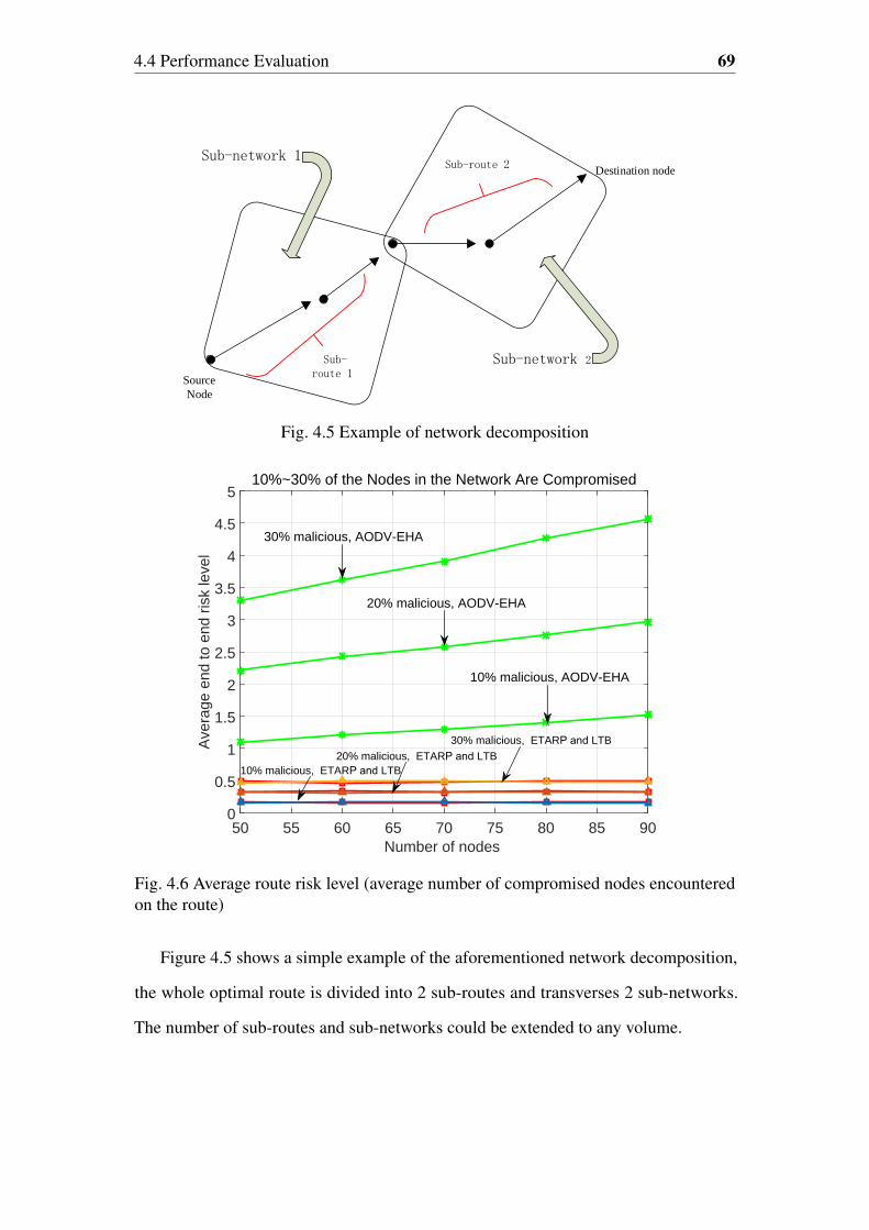
4.4 Performance Evaluation 69
Sub-network 1
Sub-network 2Sub- route 1
Sub-route 2
Source
Node
Destination node
Fig. 4.5 Example of network decomposition
Number of nodes 50 55 60 65 70 75 80 85 90
Ave
rage
end
to e
nd r
isk
leve
l
0
0.5
1
1.5
2
2.5
3
3.5
4
4.5
510%~30% of the Nodes in the Network Are Compromised
10% malicious, AODV-EHA
20% malicious, AODV-EHA
30% malicious, AODV-EHA
20% malicious, ETARP and LTB 10% malicious, ETARP and LTB
30% malicious, ETARP and LTB
Fig. 4.6 Average route risk level (average number of compromised nodes encounteredon the route)
Figure 4.5 shows a simple example of the aforementioned network decomposition,
the whole optimal route is divided into 2 sub-routes and transverses 2 sub-networks.
The number of sub-routes and sub-networks could be extended to any volume.

4.4 Performance Evaluation 70
Safety Performance
Figure 4.6 shows the safety performance of the 3 protocols under different compromised
ratios (10% – 30%).
Remark. The number of compromised node in the network is closely related to the
attacker’s subjective intention of paralysing the network, and in some sense it is un-
predictable. The authors in [5] figure out that, for an unspecific (unknown) type of
attack against WSNs, if no more than 20% of the nodes are malicious, the attack can
be detected and confined, which is due to the fact that the great majority of nodes are
still behaving properly and it is not complicated to distinguish the misbehaving ones. In
some other research studying security of WSNs, the numbers of malicious nodes in their
simulations are usually assumed to be 1% – 30% of the total number of sensor nodes in
the network [30, 43, 60].
The upper three lines, from top to bottom, denote the safety performance of AODV-
EHA, with the compromised ratio from 30% down to 10%. The lower three pairs of
inter-weaved lines, from top to bottom, represent the safety performance of ETARP and
LTB-AODV, at the compromised ratio from 30% down to 10%. It can be seen that, as
the malicious ratio increases from 10 % to 30 %, the difficulty of maintaining security
in the network is increasing. On the other hand, under different malicious ratios, the
safety performance lines of ETARP and LTB-AODV wind around each other while
fluctuating a little bit as the nodes number increase. Therefore, we can conclude that
ETARP can maintain a similar safety performance as LTB-AODV.
By comparison, there is a more notable increment of risk level (average number
of compromised nodes expected to encountered on the route) for AODV-EHA, as the
malicious ratio increases in the network. Under any certain malicious ratio, the risk
level line for AODV-EHA keeps increasing with the number of nodes in the network.
This is due to the fact that network coverage area remaining the same while the number
of compromised nodes increases. Thus, we can conclude that there is no security in
AODV-EHA, as expected since its original design did not take safety into consideration.

4.4 Performance Evaluation 71
Number of nodes 50 55 60 65 70 75 80 85 90
Ave
rage
end
to e
nd tr
ansm
issi
on c
ost (
Joul
e)
#10-3
0
1
2
3
4
5
6
710% of the Nodes in the Network Are Compromised
ETARPLTBAODV-EHA
Fig. 4.7 Average end to end transmission cost (Joule)
Number of nodes 50 55 60 65 70 75 80 85 90
Ave
rage
end
to e
nd tr
ansm
issi
on c
ost (
Joul
e)
#10-3
0
1
2
3
4
5
620% of the Nodes in the Network Are Compromised
ETARP LTBAODV-EHA
Fig. 4.8 Average end to end transmission cost (Joule)
Energy Efficiency Performance
Figure 4.7 – 4.9 show the average energy cost of each transmission under different
compromised ratios (10% – 30%).

4.4 Performance Evaluation 72
Number of nodes 50 55 60 65 70 75 80 85 90
Ave
rage
end
to e
nd tr
ansm
issi
on c
ost (
Joul
e)
#10-3
0
1
2
3
4
5
630% of the Nodes in the Network Are Compromised
ETARPLTBAODV-EHA
Fig. 4.9 Average end to end transmission cost (Joule)
For any certain malicious ratio, both lines of ETARP and LTB-AODV fluctuate per
number of nodes in the network. ETARP consistently uses less average transmission
cost compared to LTB-AODV in terms of energy. More specifically, the energy cost of
ETARP is reduced by 2.4% to 20.5% in comparison to that of LTB-AODV, depending on
various situations. But there is no clear increase or decrease tendency of the energy cost
as the nodes number ascends. In honest scenarios, usually the average transmission cost
is inverse proportional to nodes number. It is because the increment of nodes density
provides more choices of nodes, and is more likely to find a more energy efficient route.
But in our case, as the malicious ratio is constant, more nodes means not only more
potential routes, but also more compromised nodes existing in the network. Since route
discovery tries to avoid comprising malicious node, therefore the energy efficiency, to
some extent, is sacrificed sometimes.
By comparison, the average transmission cost of AODV-EHA under any certain
malicious ratio tends to decrease as the nodes number increase. The cost appears to be
less than that of ETARP or LTB-AODV, but as illustrated in Section 4.4.3, the route
determined by AODV-EHA is likely to be a dead link almost in every transmission.

4.4 Performance Evaluation 73
50 55 60 65 70 75 80 85 90Number of nodes
1
2
3
4
5
6
7
8
9
Ave
rage
end
to e
nd d
ista
nce
(Hop
s)
10% of the Nodes in the Network Are Compromised
LTBETARPAODV-EHA
LTB and ETARP
Fig. 4.10 Average route length (hops) versus the number of nodes
A dead link makes the theoretical minimum energy cost of AODV-EHA meaningless,
since the packets are probably dropped on their way without reaching the destination.
All the energy already spent on the transmissions are wasted, even though it is ostensibly
less than that of ETARP.
Average Route Length
Under AODV-EHA, the route length is increasingly high as the number of nodes in the
area goes up (it is because the increment of nodes density provides more choices of
nodes, and is more likely to find a more energy efficient route at the price of longer route
length), while that of LTB-AODV and ETARP are relatively stable, as can be seen from
Figure 4.10 – 4.12. It can also be seen that regardless of compromised ratios, there is no
clear difference in route length between LTB-AODV and ETARP as the nodes number
ascends. This is because both LTB-AODV and ETARP are designed to be secure, they
try not to involve any compromised node in route discovery. In addition, ETARP does
not pay any special attention on minimizing route length. Therefore, under any certain
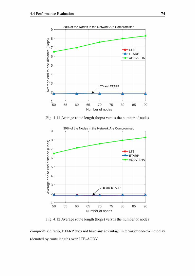
4.4 Performance Evaluation 74
50 55 60 65 70 75 80 85 90Number of nodes
1
2
3
4
5
6
7
8
9
Ave
rage
end
to e
nd d
ista
nce
(Hop
s)
20% of the Nodes in the Network Are Compromised
LTBETARPAODV-EHA
LTB and ETARP
Fig. 4.11 Average route length (hops) versus the number of nodes
50 55 60 65 70 75 80 85 90Number of nodes
1
2
3
4
5
6
7
8
9
Ave
rage
end
to e
nd d
ista
nce
(Hop
s)
30% of the Nodes in the Network Are Compromised
LTBETARPAODV-EHA
LTB and ETARP
Fig. 4.12 Average route length (hops) versus the number of nodes
compromised ratio, ETARP does not have any advantage in terms of end-to-end delay
(denoted by route length) over LTB-AODV.

4.5 Summary 75
From all the above results gained about different performances, we can conclude
that under different compromised ratios, ETARP has advantages in terms of energy
efficiency in transmission while it can still maintain almost the same safety performance
as LTB-AODV at the same time (stated in Section 4.4.3). But ETARP has no clear
advantage over LTB-AODV in terms of end-to-end delay. By comparison, even though
AODV-EHA achieves the theoretical “lowest” transmission cost, there is no security in
AODV-EHA since its original design focused on reducing energy cost but did not give
attention to security.
4.5 Summary
In this chapter, we proposed the ETARP routing protocol for WSN applications operat-
ing in extreme environments usually for military use, such as SDT and ASW. ETARP
simultaneously considers energy efficiency and security concerns by taking advantage
of utility theory. Through simulations, we evaluated the energy efficiency performance
and safety performance of ETARP in comparison to LTB-AODV and AODV-EHA.
Results show that although AODV-EHA has the theoretical “lowest” transmission cost,
there is no security in it, while ETARP has the advantages in terms of energy effi-
ciency in transmission while it can still maintain about the same safety performance as
LTB-AODV.

Chapter 5
Vampire Attacks Detection and
Defence
5.1 Introduction
In this chapter, RCPED protocol, is proposed to protect routing protocols from Vampire
attacks that have been introduced in Chapter 1. Compare to the existing solutions, our
approach is independent of cryptographic methods, which can avoid extra computation
cost, transmission cost and even hardware (used for encryption purpose). These ad-
vantages are quite meaningful as the wireless sensors are with limited size, computing
capability and battery.
The nominated scenario in this chapter can be considered as the application of
environment surveillance. The engineer just stays at a fixed observation point (location
is decided by the engineer) in the region covered by the deployed WSN, and collects
data from the nodes.
In Section 5.2 and Section 5.3, a procedure for detection of Vampire attacks is
described in detail. Section 5.4 discusses how to mitigate the harm from Vampire
attacks. Performance evaluation of the proposed solution in terms of simulation results
is presented in Section 5.5.

5.2 General Concept and Passive Detection 77
5.2 General Concept and Passive Detection
The general approach of RCPED against Vampire attacks is illustrated in Figure 5.1. It
consists of passive detection (further addressed in Section 5.2.1 and Section 5.2.2), and
active detection (further addressed in Section 5.3).
The proposed solution in this chapter is designed to reduce the cost (e.g. energy),
it would be resource consuming if initiating the active detection on malicious nodes
directly. Therefore we only let passive detection with less cost of resource in operation
at the very beginning. Passive detection is integrated in the normal routing process and
continually monitors the network, with no significant additional actions. Similar to
any on-demand solution, active detection remains silence until any suspicious sign is
captured by passive detection. If active detection is triggered, it tries to identify which
nodes are possibly participating in any Vampire attacks. Nodes in the network are
alerted afterwards, to stop suspicious nodes from involving in the route discovery of
any future data transmission.
Previous work in [31] shows that the approximate cost of transmitting a data packet
from an arbitrary node in the network to a stationary observation point (denoted by
E(M)) has a functional relationship with the number of nodes in the network (denoted
by M). If the relationship between the transmission cost and density of nodes in the
network can be determined, the expected average transmission cost corresponding to a
specific nodes density in the “normal case” (when no attacks against the network are
happening) can be figured out as well.
Provided that the task described above is done, we can track the data transmissions
in the network and calculate the energy cost of incoming packets at the observation
point. If the average of these recorded costs is significantly higher than the expected
value for the “normal case”, then an attack may be suspected. This process is called
passive detection because it involves measurements that do not interfere with the normal
operation of the network. Passive detection is a type of anomaly detection [14] which
refers to the process of looking for abnormal behaviour (in this case, behaviour of the

5.2 General Concept and Passive Detection 78
Normal route determination and
passive detection on going
Suspicious behaviour detected?
Active detection triggered
Collect security-related info. of nodes
Aggregation of collected info. and
change routes in future transmissions
Risk on nodes still tracked by active
detection?
No
Yes
No
Yes
Fig. 5.1 General concept of detection and protection against of Vampire attacks
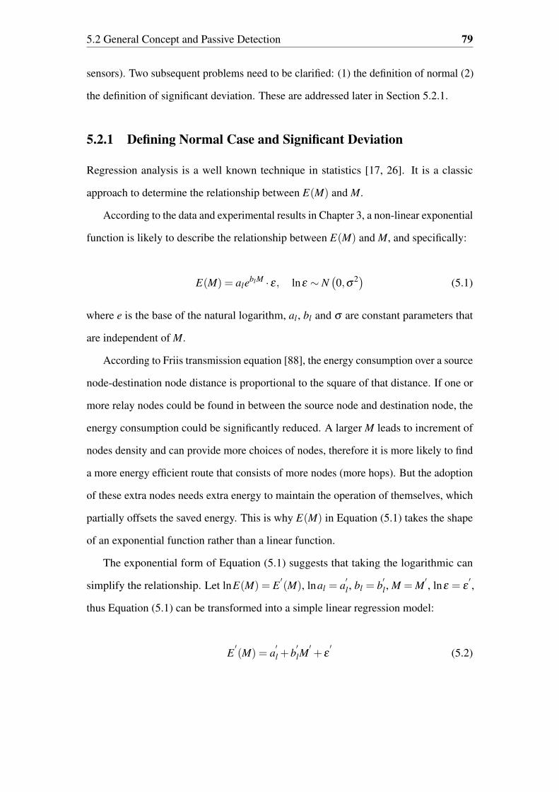
5.2 General Concept and Passive Detection 79
sensors). Two subsequent problems need to be clarified: (1) the definition of normal (2)
the definition of significant deviation. These are addressed later in Section 5.2.1.
5.2.1 Defining Normal Case and Significant Deviation
Regression analysis is a well known technique in statistics [17, 26]. It is a classic
approach to determine the relationship between E(M) and M.
According to the data and experimental results in Chapter 3, a non-linear exponential
function is likely to describe the relationship between E(M) and M, and specifically:
E(M) = aleblM · ε, lnε ∼ N(0,σ2) (5.1)
where e is the base of the natural logarithm, al , bl and σ are constant parameters that
are independent of M.
According to Friis transmission equation [88], the energy consumption over a source
node-destination node distance is proportional to the square of that distance. If one or
more relay nodes could be found in between the source node and destination node, the
energy consumption could be significantly reduced. A larger M leads to increment of
nodes density and can provide more choices of nodes, therefore it is more likely to find
a more energy efficient route that consists of more nodes (more hops). But the adoption
of these extra nodes needs extra energy to maintain the operation of themselves, which
partially offsets the saved energy. This is why E(M) in Equation (5.1) takes the shape
of an exponential function rather than a linear function.
The exponential form of Equation (5.1) suggests that taking the logarithmic can
simplify the relationship. Let lnE(M) = E′(M), lnal = a
′l , bl = b
′l , M = M
′, lnε = ε
′,
thus Equation (5.1) can be transformed into a simple linear regression model:
E′(M) = a
′l +b
′lM′+ ε
′(5.2)

5.2 General Concept and Passive Detection 80
Next, estimates of al (or a′l) and bl (or b
′l), denoted by al (or a′l) and bl (or b′l ), can
be determined by linear regression given a set of past records of M and corresponding
E(M). Details of how the records can be acquired are described in [31].
As addressed in [110], if Vampire attacks targeting stateless routing protocols
are underway, simulation results show that on average, a randomly located attacker
in a network with randomly generated topology, can increase the network energy
consumption by a factor of 1.48±0.99 if the adversary performs a carousel (route loop)
attack, and by a factor of 2.67±2.49 if the adversary performs stretch attack. The large
standard deviation is because the length of the adversarial path length is affected by the
position of the attacker in relation to the source or destination node. Higher network
energy usage increment leads to higher possibility of Vampire attacks in operation. In
worst case this number may go up to a factor of 3.96 by carousel attack, or up to 10.5
by stretch attack.
Therefore we can keep checking the expected transmission cost of any incoming
packet, if there is any unnormal increment as discussed in the previous paragraph, the
network is potentially experiencing a Vampire attack. Then the active detection phase is
triggered, details is addressed later in Section 5.3 and Section 5.4.
All incoming data packets can carry information about their travelled route by
carrying a list of encountered nodes together with their location information (nodes
localisation is discussed in Section 5.2.2), these routes information are essential for the
calculation of expected transmission cost of packet delivery mentioned in the previous
paragraph (estimation details are given in Section 5.2.2). Note that the transmission
of these location information can cost a bit more than that of standard packet, this
need to be taken into consideration in later evaluation. According to the NMEA-
0183V20 standards [75] formulated by the National Marine Electronics Association
of USA, a typical GPS positioning information accounts for 88 byte, but most of the
information (such as velocity and magnetic declination) can be consider as redundant in
our application, only the coordinates information are retained.

5.2 General Concept and Passive Detection 81
5.2.2 Practical Issues in Passive Detection
As discussed in Section 5.2.1, in passive detection, expected transmission cost of
incoming packets need to be determined. Furthermore, the determination process needs
locations of nodes on the route that those packets travelled through. Details on how to
solve these practical issues are given in this section.
Estimation of Transmission Cost on a Specific Route
On any chosen route i spanning a total number of Ji nodes, the expected total transmis-
sion cost E(i) in terms of energy can be calculated as [31]:
E(i) = E(i,1)+E(i,2)+ ...+E(i,Ji−1) (5.3)
where E(i,m) is the estimated transmission cost from the m-th node on this route to
its next hop (1≤ m≤ Ji−1). More details of the above calculations can be found in
Section 3.2.3.
Node Localisation
GPS is the most obvious means to establish the locations of nodes. In order to reduce
overhead, most localization systems use one or more anchor nodes equipped with GPS
chip instead of including GPS in every node [52]. These anchor nodes broadcast their
current positions periodically to sensor nodes to estimate their locations.
For the long-term monitoring application under consideration, since nodes in the
network usually unreachable after deployment, battery life is the major constraint. A
high updating frequency such as one sample per second is meaningless when monitoring
weekly or even monthly. A push-to-fix mode has been suggested for long-term operating
applications [89] which means the GPS is put to sleep most of time and position is
only updated at regular time intervals (every 2 hours or even longer). This mode can
be useful for GPS embedded nodes. For our application, nodes rarely change their
positions therefore a longer time interval, e.g. one sample per day, is sufficient. Since

5.2 General Concept and Passive Detection 82
Anchor 1 (x1, y1)
Anchor 2 (x2, y2)
Anchor 3 (x3, y3)
Node need to be
located (x0, y0)
d1 d2
d3
Fig. 5.2 Process of trilateration
each position updating process can last for up to 30 seconds, the energy cost of a GPS
embedded node could be limited to 31.08 Joule per day [89]. If we choose a common
and cheap 18650-size cylindrical lithium-ion battery cell [38] (3.3v, 1.6-Ah), the GPS
embedded node can operate for more than one and a half years.
According to [44], trilateration approach shown in Figure 5.2 based on the received
signal strength is the most suitable for node localisation in WSNs due to its imple-
mentation simplicity and low hardware requirement. The basic idea is as follows: the
anchor nodes periodically broadcast their locations, and the nodes need to be located
can receive these information and estimate the distance from anchor nodes by measuring
the received signal strength (RSS). Suppose the coordinates of anchor nodes 1, 2, 3 are
(x1,y1), (x2,y2), (x3,y3), the coordinates of the node need to be located is (x0,y0), and
the distances between three anchor nodes to the node to be located are d1, d2, d3. If
we choose (x1,y1), (x2,y2), (x3,y3) as centres and draw 3 circles with radius d1, d2, d3,
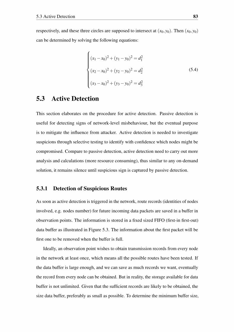
5.3 Active Detection 83
respectively, and these three circles are supposed to intersect at (x0,y0). Then (x0,y0)
can be determined by solving the following equations:
(x1− x0)2 +(y1− y0)
2 = d21
(x2− x0)2 +(y2− y0)
2 = d22
(x3− x0)2 +(y3− y0)
2 = d23
(5.4)
5.3 Active Detection
This section elaborates on the procedure for active detection. Passive detection is
useful for detecting signs of network-level misbehaviour, but the eventual purpose
is to mitigate the influence from attacker. Active detection is needed to investigate
suspicions through selective testing to identify with confidence which nodes might be
compromised. Compare to passive detection, active detection need to carry out more
analysis and calculations (more resource consuming), thus similar to any on-demand
solution, it remains silence until suspicious sign is captured by passive detection.
5.3.1 Detection of Suspicious Routes
As soon as active detection is triggered in the network, route records (identities of nodes
involved, e.g. nodes number) for future incoming data packets are saved in a buffer in
observation points. The information is stored in a fixed sized FIFO (first-in first-out)
data buffer as illustrated in Figure 5.3. The information about the first packet will be
first one to be removed when the buffer is full.
Ideally, an observation point wishes to obtain transmission records from every node
in the network at least once, which means all the possible routes have been tested. If
the data buffer is large enough, and we can save as much records we want, eventually
the record from every node can be obtained. But in reality, the storage available for data
buffer is not unlimited. Given that the sufficient records are likely to be obtained, the
size data buffer, preferably as small as possible. To determine the minimum buffer size,

5.3 Active Detection 84
4, 23, 14, … …
3, 5, 17, … …
Enqueue
Dequeue
The data buffer
stores I.D. info.
of nodes that
incoming
packets travelled
through
I.D. info. of
nodes that last
incoming
packet
travelled
through
I.D info. of
nodes that first
incoming
packet
travelled
through
Fig. 5.3 Format of data buffer
we define the event needs to be fulfilled: every node in the network has transmitted data
to observation point at least once. Suppose after kt transmissions exercised (means kt
transmission records are saved in buffer), this event is satisfied at the probability of Pe,
thus the probability of its complementary event (transmission from a specific node has
never been recorded) is below (1−Pe):
(M−1
M
)kt
≤ 1−Pe (5.5)
where M is the number of nodes in the network, M−1M is the probability that the trans-
mission record of any specific node has not been obtained (assume that the probability
of any node in the network communicates with observation point is equal), thus kt has
to satisfy
kt ≤log(1−Pe)
log(M−1
M
) (5.6)
5.3 Active Detection 85
Therefore, the minimum size of the buffer is⌈
log0.01log(M−1
M )
⌉, where ⌈ ⌉ is the Ceil
function. For example, if Pe = 0.99, nodes number M = 50, the minimum size of data
buffer would be⌈
log0.01log( 50−1
50 )
⌉= 228.
Inspired by the route rebuilding concept discussed in [20], suppose all the informa-
tion of suspicious routes that are found in buffer are denoted by B1,B2, ...,BNb , where
Nb is the total number of detected suspicious routes from the buffer. Thus we can build
a comprehensive vector B as follows:
B = [B1,B2, ...,BNb ] (5.7)
we further define any specific row in B as BV = {Vm : 1 ≤ m ≤ |BV |} , where Vm
represents each node on this route BT , and V is an integer and 1≤V ≤ Nb (| | means
the number of elements in set).
Note that the data buffer is not static, as transmissions going on, the data buffer is
updating itself all the time. Thus B, which is extracted form the data buffer is a “live”
vector and updating itself actively as time goes by.
5.3.2 Detection of Route Loop Attackers (Carousel Attackers)
If no route loop is formulated, a specific packet is expected to travel through every node
on the route only once. If a node appears multiple times in a single route BL, a route
loop is probably exists. And those nodes are marked as suspicious nodes and further
investigated(details are further addressed in Section 5.4.1).
Note the mark is not constant. As mentioned in Section 5.3.1, the B is updating
itself constantly, so the mark on a node may vary from time to time.
5.3.3 Detection of Route Stretch Attackers
If a node does not appears in a single line multiple times in B, but more than once in
multiple BL instead, it is probably been part of formulating stretched route. It is then

5.4 Protection Against Vampire Attacks in Routing 86
Node is Not
Compromised?
(H)
Been Part of a
Route Loop?
(L)
Been Part of a
Stretched
Route?
(S)
Fig. 5.4 Bayesian network for information aggregation
marked as a suspicious node and further investigated (details are further addressed in
Section 5.4.1 ).
As already been explained in Section 5.3.2, these marks are not static due to B is
updating itself.
5.4 Protection Against Vampire Attacks in Routing
As described in Figure 5.1 of Section 5.2, the security related data obtained from Section
5.3 should be fed back to route discovery in order to mitigate the damage caused by
malicious nodes.
5.4.1 Monitoring Information Aggregation
Based on the information gathered from the aforementioned detections, it is possible
and necessary to calculate a “belief” about a suspicious node’s trustworthiness. Since
the suspicious nodes might be part of carousel attack or stretch attack or both (more than
one suspicious behaviour), here a Bayesian learning network is employed to aggregate
and analyse the collected information. A general introduction of the Bayesian network
and why it is employed have been given in Section 4.3.3.

5.4 Protection Against Vampire Attacks in Routing 87
Table 5.1 Incomplete data sets D
D H L Sobservation1 ? F Tobservation2 ? T Fobservation3 ? T T
Table 5.2 Initial estimates
H F(h)T 0.8F 0.2
H L F(l|h)T T 0.1T F 0.9F T 0.8F F 0.2
H S F(s|h)T T 0.1T F 0.9F T 0.9F F 0.1
Similar to Section 4.3.3, the practical Bayesian network employed here is shown in
Figure 5.4, the purpose is to determine a node’s “health” status (node is compromised or
not), denoted by variable H, two symptoms are considered: “node is part of a route loop”
(denoted by variable L), and “route is part of a stretched route” (denoted by variable S).
These variables are binary, represented by T (true) or F (false) for variable H, L and S.
Table 5.1 shows an example of incomplete data sets D with 3 different recorded
data cases: observation1, observation2 and observation3. A data case is a record of
a set of symptoms shown by a node, in other word, a record with certain combination
of instantiation (h, l, s), in which the symptom parameters (h, l,s) = (T,T,T ) denote
that this node has not been compromised, used to be a part of route loop and a stretched
route before, respectively. And (h, l,s) = (F,F,F) denote that this node has been
compromised, not used to be a part of route loop as well as stretched route before,
respectively. The symbol “?” represents the missing values of variables.
The goal is to calculate the expected empirical distribution of nodes status H based
on the incomplete data set. Some initial estimates are assumed as shown in Table 5.2
based on common sense; e.g. a comprised node is more likely to be part of a route loop
or stretched route in previous routing.
The expected empirical distribution of the incomplete data set D is defined as:
FD (αt)def=
1Nds
∑observationi,ci=αt
F (ci|observationi) (5.8)

5.4 Protection Against Vampire Attacks in Routing 88
where αt is an event with certain combination of instantiation (h, l,s), Nds is the size of
the data set, and ci are variables with unrecorded values of case observationi.
For example, the probability of an instantiation (h, l,s) = (T,F,T ) (denotes node is
not compromised, node did not use to be part of route loop and node used to be part of
stretched route in routing before) is given by
FD (h = T, l = F,s = T ) =F (h = T |observation1)
3(5.9)
Repeating this process can obtain the probability of all the other instantiations
(h, l,s). Then the expectation maximization estimate of a node not been compromised
is written as
FD (h = T ) = ∑l,s
F (h = T, l,s) (5.10)
where l and s denote all possible values of l and s, respectively. Other parameters such
as FD (l|h) and FD (s|h) can be calculated by
FD (l|h) = FD (h, l)FD (h)
(5.11)
FD (s|h) = FD (h,s)FD (h)
(5.12)
All the results derived from (5.8), (5.11) and (5.12) based on incomplete data sets
D constitute the D estimates that serve as the replacement of initial estimates shown in
Table 5.2.
As mentioned in Section 5.3.2, the B is an “live” vector, therefore we can keep
observing the nodes symptoms from B and periodically fetch new incomplete data sets
D1, D2 ... Dm where m is a positive integer. If we keep fetching data from B, we can
get estimates with higher likelihood [25].
5.4 Protection Against Vampire Attacks in Routing 89
5.4.2 Security Information Distribution
The aforementioned security information calculated from Section 5.4.1 (which nodes
are likely to be compromised, together with the probability of being compromised),
need to be forwarded to the nodes in the network, for the purpose of a safer route
discovery. For the sake of energy efficiency, rather than directly flooding security
related information through the entire network, they are passed to certain “cluster heads”
first, and then broadcast to surrounding nodes [120]. Nodes in the network can then take
advantage of this information to select routes avoiding malicious nodes. In our case,
the anchor nodes which have been formerly used for nodes localization (see Section
5.2.2 for more details), naturally become “cluster heads” for the purpose of distributing
security related information, since they are:
• Less vulnerable than any normal node in the network, for they do not directly
participate in data transmissions (output only);
• Already deployed in the network, it would be more economic (in terms of both
energy and cost) to add some non-heavy duty task to them rather than deploying
additional nodes for information distribution.
5.4.3 Route Discovery Based on AHP
After the security information have been distributed around the network, the next step
is to utilize these information to discover the optimal routes with the help of Analytic
Hierarchy Process (AHP) [41]. AHP is one choice of multi-criteria decision analysis
(MCDA) methods, which are developed to help making decisions (in our case, choosing
the best route) under multiple concerns (e.g. energy efficiency, security). There are
other candidates besides AHP, but none of those candidates (including AHP) is perfect
and cannot be applied to all problems.
In the case of this chapter, the “utility function” (which has been introduced in
Section 4.3.2) of each route is hard to construct. It is because the Vampire attackers still
deliver the packet eventually, thus in a sense, the energy consumed by attackers cannot

5.4 Protection Against Vampire Attacks in Routing 90
be considered as “completely” wasted. Furthermore, as addressed in Section 5.2.1,
the extra energy consumption caused by Vampire attacks depends on some random
parameters, it varies a lot and its exact volume is hard to estimate, which brings even
more difficulties for constructing the utility function. As suggested by the authors of
[41], AHP is particularly useful when the decision maker is unable to construct a utility
function.
Then we can set the goal to find out the optimal route based on multiple criteria, as
shown in Figure 5.5. The top element is the goal of the decision, the second level of
the hierarchy represents the criteria, the lowest level represents the available choices
(routes). Following this figure, the scores, or so called priorities, of different choices
of routes, are calculated based on the pairwise comparisons between different criteria
provided by user.
5.4.4 Details of AHP
In AHP, pairwise comparisons are made between different criteria, thus ratio scales are
needed. The judgement is a relative value or a quotient w1/w2 of two quantities w1 and
w2 (in our case w1 and w2 are security concern and energy efficiency concern). In other
words, these relative values (or ratio scales) represent the priority (importance) of each
criterion.
Table 5.3 shows the most straightforward linear priority setup proposed by Saaty
[93]. There are 9 degrees of priority because a human being cannot simultaneously
compare more than 7 subjects (±2) [68], i.e. we are unable to assign proper importance
to more than 7 items (±2). This is the limitation of human being when processing
information. To avoid confusion, we choose 7 + 2 = 9 degrees.
There are other choices as shown in Table 5.4. All these choice are based on
psychophysics theory. The validity of each one in decision making is usually evaluated
by experiments. In fact which scale provides the best performance is controversial,
experiments results reveal that they are better than the basic linear one [64, 87, 96].

5.4 Protection Against Vampire Attacks in Routing 91
Level 1
Determination of Optimal Route
Level 2
Level 3
Energy CostActive Detection
Results
Route 1
Route 2
Route N
Route 1
Route 2
Route N
…
…
…
…
Fig. 5.5 Problem structure
Example: consider two routes evaluated according to two criteria, the energy
efficiency and safety level. The security concern is considered twice as important
as the energy efficiency. Suppose Route 2 is 2.5 times as safe as Route 1, and with
transmission cost that is double compared to Route 1. The two routes can be compared
on a ratio scale:
Route 2Route 1
= 2 · 100%40 %
+50%
100%= 5.5 (5.13)
Therefore, Route 2 is 5.5 times as good as Route 1.

5.4 Protection Against Vampire Attacks in Routing 92
Table 5.3 Degree of priority (importance)
Degree of Importance Definition1 Equal Importance2 Weak3 Moderate Importance4 Moderate Plus5 Strong Importance6 Strong Plus7 Very Strong or demonstrated Importance8 Very Very Strong9 Extreme Importance
Table 5.4 Different scales of priority setup
Scale Types Equ
alIm
port
ance
Wea
k
Mod
erat
eIm
port
ance
Mod
erat
ePl
us
Stro
ngIm
port
ance
Stro
ngPl
us
Ver
ySt
rong
Impo
rtan
ce
Ver
yV
ery
Stro
ng
Ext
rem
eIm
port
ance
Linear 1 2 3 4 5 6 7 8 9Power 1 4 9 16 25 36 49 64 81Geometric 1 2 4 8 16 32 64 128 256Logarithmic 1 1.58 2 2.32 2.58 2.81 3 3.17 3.32Square Root 1 1.41 1.73 2 2.23 2.45 2.65 2.83 3Asymptotical 0 0.12 0.24 0.36 0.46 0.55 0.63 0.70 0.76Inverse Linear 1 1.13 1.29 1.5 1.8 2.25 3 4.5 9Balanced 1 1.22 1.5 1.86 2.33 3 4 5.67 9
For an interval scale as below:
Route 2−Route 1 = 2 · (100%−40%)+(50%−100%) = 0.7 (5.14)
This also shows Route 2 is better.
To derive priorities of each route, verbal comparisons must be converted to numerical
ones; details are given in the Section 5.4.5.
5.4.5 Priority Calculation in Optimal Route Determination
Suppose on any chosen i-th route with total number of Ji nodes, the expected total
priority Py(i) can be calculated as
Py(i) = Py(i,1)+Py(i,2)+ ...+Py(i,Ji−1)) (5.15)
5.4 Protection Against Vampire Attacks in Routing 93
where Py(i,m) is the priority from the m-th node on this route to its next hop (1≤ m≤
Ji−1).
In order to judge different routes fairly, a “standard next hop” is defined: the next
hop node is 100% not compromised, the distance to next hop node is the maximum
radio range, and the transmission cost after a successful packet delivery to next hop
node is Est .
Similar to the example given in Section 5.4.4, the priority on each hop compare to
the case of ’standard next hop’ is further given by
Py(i,m) = Pey(i,m)+ Is ·Psy(i,m) (5.16)
where Pey(i,m) is the priority (importance) of energy efficiency, inversely proportional
to the normalised expected transmission cost (with respect to Est , and please see Section
3.2.3 for how to estimate the transmission cost). Similarly, Psy(i,m) is the priority
(importance) of security concerns, proportional to the possibility that the next hop
node is not compromised (derived from Equation (5.10) in Section 5.4.1). Is is the
corresponding scale of security concern priority, indicating that security concern is
considered Is times as important as the energy efficiency concern. The exact volume of
Is could be picked from Table 5.4.
5.4.6 Optimal Route Determination
The optimal route is chosen with the maximum Py interpreted as the safest route while
keeping the least energy consumption possible.
Practical route discovery can be accomplished with existing routing protocols (such
as AODV), with minor changes in the control messages such as RREQs and RREPs.
Specifically, the field “hop count” should be replaced with corresponding “priority
volume count”. In RREQs, the “priority volume count” implies the total priority volume
of the route from the originator node to the node handling the request. In RREPs,
“priority volume count” denotes the priority volume of the route from originator node to
5.5 Simulation Results 94
the destination node. There is another minor change as well: AODV picks the route
with minimum hops, the optimal route here is with the maximum priority volume.
5.5 Simulation Results
In this section, the performance of the RCPED routing protocol is analysed. Two
competitors are chosen for comparison. The first protocol for comparison is PLGPa,
which is dedicated to the mitigation of Vampire attacks based on the cryptographic
approach. The other protocol for comparison is AODV-EHA, an energy efficient
protocol aware of energy harvesting [31].
Overview of PLGPa
PLGP is a clean-slate secure sensor network routing protocol proposed by Parno et al.
[78]. It consists of two phrases: topology discovery and packet forwarding. In the first
phrase, all the nodes are organized in a tree, which can be further used for addressing
and routing. In the second phrase, after transmission is initiated, each node chooses the
node with maximum “logical distance (determined from the aforementioned tree)” from
the source node as the next hop, which is aimed to make sure that the next hop would
be closer to the destination node (in other words, try to shorten the logical distance to
the destination as much as possible). PLGPa [110], a modified version of PLGP, can
additionally provide the “no-backtracking” feature that can resist the Vampire attacks,
at the cost of additional energy consumption caused by encryption.
Overview of AODV-EHA
An overview of AODV-EHA was given in Section 4.4.1.

5.5 Simulation Results 95
Table 5.5 Simulation parameters
Parameters DescriptionsSimulation Area 500 m × 500 m
Node Radio Range 250 mTraffic Type CBRPacket Size 127 bytesData Rate 20 kbps
Signal to Noise Ratio (SNR) Threshold β 10Processing Power Level Pc 10−4 WReceiving Power Level Pr 5×10⁻⁵ W
Outage Requirement P∗out(i,m) 10−4
5.5.1 Simulation Setup
The experimental evaluation is carried out by means of MATLAB simulations using
the Monte-Carlo method. The criteria considered is the overall cost in which safety
performance, average route length and energy efficiency performance are involved.
The size of the simulated area is 500 m×500 m. The communication range of each
node is 250 m. Considering the WSN applications that are the focus of this chapter (as
addressed in the beginning of Section 5.1), IEEE 802.15.4 is chosen for the physical and
data link layer, which is suitable for low data rate but very long battery life applications
[39]. According to the specification mentioned in [39], the traffic type is CBR with a
data rate of 20 Kbps, and the size of each packet is 127 bytes. Since the transmission
cost prediction partly depends on previous work [95], therefore for those parameters
required for the prediction process we continue to use same values as adopted in [95].
Details are listed in Table 5.5.
Every simulation contains a certain malicious fraction of the network nodes. These
compromised nodes are located randomly in the simulation area, and they are assigned
with certain behaviours that can further affect the route discovery process.
The destination node is assumed to be stationary, which complies the scenario in
applications of enemy detection or environment surveillance, the engineer just stay at
a fixed observation point in the region where the WSN is deployed, and collects data
from the nodes. The nodes number varies from 60 to 200.
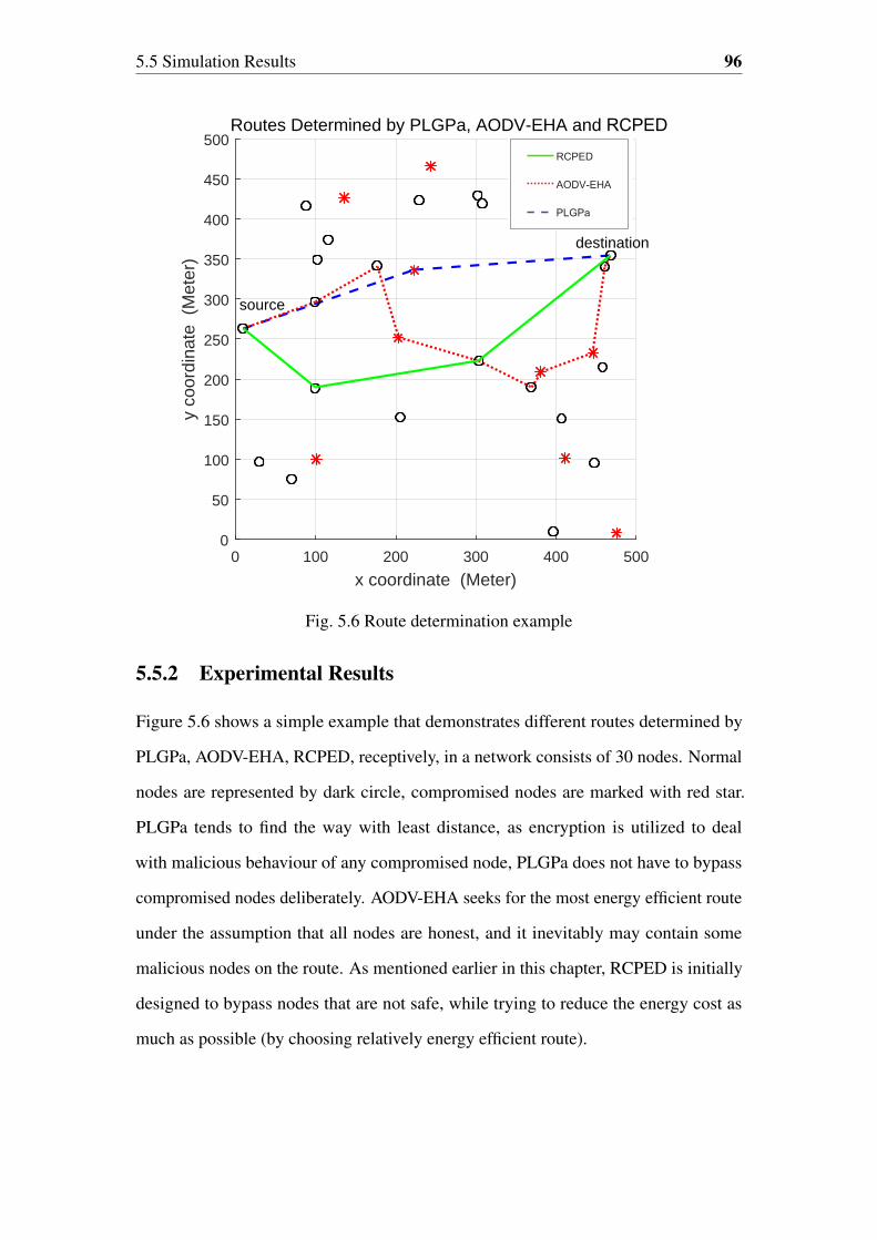
5.5 Simulation Results 96
0 100 200 300 400 500
x coordinate (Meter)
0
50
100
150
200
250
300
350
400
450
500
y co
ordi
nate
(M
eter
)
Routes Determined by PLGPa, AODV-EHA and RCPED
source
destination
Fig. 5.6 Route determination example
5.5.2 Experimental Results
Figure 5.6 shows a simple example that demonstrates different routes determined by
PLGPa, AODV-EHA, RCPED, receptively, in a network consists of 30 nodes. Normal
nodes are represented by dark circle, compromised nodes are marked with red star.
PLGPa tends to find the way with least distance, as encryption is utilized to deal
with malicious behaviour of any compromised node, PLGPa does not have to bypass
compromised nodes deliberately. AODV-EHA seeks for the most energy efficient route
under the assumption that all nodes are honest, and it inevitably may contain some
malicious nodes on the route. As mentioned earlier in this chapter, RCPED is initially
designed to bypass nodes that are not safe, while trying to reduce the energy cost as
much as possible (by choosing relatively energy efficient route).

5.5 Simulation Results 97
60 80 100 120 140 160 180 200
Number of nodes
0
0.005
0.01
0.015
0.02
0.025
0.03
Ave
rage
end
to e
nd tr
ansm
issi
on c
ost (
Joul
e)
10% of the Nodes in the Network Are Compromised
PLGPaRCPEDAODV-EHA
Fig. 5.7 Average end to end overall transmission cost (Joule)
60 80 100 120 140 160 180 200
Number of nodes
0
0.005
0.01
0.015
0.02
0.025
0.03
0.035
0.04
Ave
rage
end
to e
nd tr
ansm
issi
on c
ost (
Joul
e)
20% of the Nodes in the Network Are Compromised
PLGPaRCPEDAODV-EHA
Fig. 5.8 Average end to end transmission cost (Joule)
Energy Efficiency Performance
Figure 5.7 – 5.9 show the average energy cost of each transmission (from arbitrary node
to the observation point) at different malicious ratios (10% – 30%).

5.5 Simulation Results 98
60 80 100 120 140 160 180 200
Number of nodes
0
0.01
0.02
0.03
0.04
0.05
0.06
Ave
rage
end
to e
nd tr
ansm
issi
on c
ost (
Joul
e)
30% of the Nodes in the Network Are Compromised
PLGPaRCPEDAODV-EHA
Fig. 5.9 Average end to end transmission cost (Joule)
For malicious ratio at 10% as shown in Figure 5.7, both lines of RCPED and
PLGPa fluctuate per number of nodes in the network. RCPED consistently uses less
average transmission cost compare to PLGPa, thanks to the fact that RCPED does
not need additional hardware to grantee security (additional hardware requires extra
energy consumption). In comparison to PLGPa, the energy cost reduced by RCPED can
reach up to 87.93%. The average transmission cost of AODV-EHA tends to decrease
as the nodes number increase, even it does fluctuate violently. The cost appears to
be less than that of PLGPa when nodes number in the network is above a certain
value (130 or higher). It is because the increment of nodes density provides more
choices of nodes, and is more likely to find a more energy efficient route. Even though
sometimes compromised nodes are included on the route (which make green line
fluctuate violently), the damage can be compensated to some extent. Hence, when the
choices of nodes are plenty enough (130 or higher), the compensation can be large
enough to make AODV-EHA provide a better performance than that of PLGPa.
As malicious ratio rises to 20% (illustrated in Figure 5.8 ), even though RCPED
is still the one with least average transmission cost, but its performance advantage

5.5 Simulation Results 99
over PLGPa begins to shrink. This is because it is more difficult for RCPED to
eliminate compromised nodes in route discovery as the malicious ratio goes up, the
aforementioned saved energy that comes with the independence of additional hardware
could be counteracted to some extent. The tendency of AODV-EHA remains the same
as that in Figure 5.7, but the transmission cost appear to be less than PLGPa only after
nodes number reaches 170 and above, which is more than 130 at malicious ratio 10%.
This is due to the fact that a larger malicious ratio make it more possible for AODV-EHA
to encounter compromised nodes in route discovery, hence the aforementioned energy
compensation that brought by the increment in choices of nodes is partially offset.
When malicious ratio goes up to 30% (as shown in Figure 5.9), energy cost reduced
by RCPED compare to PLGPa continues to drop, sometimes goes down to 28.34%.
The AODV-EHA keeps the same line tendency as previously appeared in Figure 5.7 and
Figure 5.8, but its performance never overcome PLGPa in the given nodes number span
(60 to 200). This is because, as malicious ratio continues to ascend, it is more and more
difficult for protocols that are not equipped with cryptographic encryption (e.g. RCPED
and AODV-EHA) to prevent the damage (extra energy cost) from compromised nodes.
From all the above results gained from overall energy cost performance evaluations,
we can conclude that under different malicious ratios, RCPED has advantages in terms
of overall energy cost in transmission. But its relative advantage over PLGPa tends to
decrease as the malicious ratio of the network goes up.
Safety Performance
In performance evaluation, “safety performance” has been naturally converted part of
energy efficiency performance given a specific malicious ratio, since all the damage
come with Vampire attacks present in the form of more energy consumption. Thus, the
overall cost is a comprehensive “energy overhead” which involves the estimated energy
cost after successfully delivering a data packet, plus the extra energy consumption
caused by the Vampire attacks in this transmission along the route discovered by a
specific routing protocol. In other words, higher energy consumption means longer

5.5 Simulation Results 100
average route length in data transmission. The overall cost (or so called comprehensive
“energy overhead”) mentioned earlier can be considered as an indicator of safety level
as well. Therefore, the earlier part of Section 5.5.2 has already presented an overall
performance evaluation including both energy efficiency and safety performance.
Average Route Length
The evaluation of “average route length” has been naturally converted to part of average
energy cost evaluation given a specific malicious ratio. This is because in the presence
of Vampire attacks, routes are more likely to be with unnecessarily long length if the
attacks take effect (in the form of more energy consumption). In other words, higher
energy consumption means longer average route length in data transmission. The overall
energy cost (or so called comprehensive “energy overhead”) mentioned earlier can be
considered as an indicator of route length as well. Therefore, the earlier part of Section
5.5.2 has already presented an overall performance evaluation including both energy
efficiency and average route length.
Effect of Buffer Size
Figure 5.10 – 5.12 show the performance of RCPED with different data buffer size at
various malicious ratio.
For malicious ratio at 10% as shown in Figure 5.10, the advantage of utilizing
larger buffer is not very distinct. In many cases the performance lines (represents the of
transmission cost) wind around each other. On the other hand, as the nodes number in
the network increases, the transmission costs of RCPED with different buffer size are
with decreasing tendency, but fluctuations (sometimes violent) still exist.
As malicious ratio rises to 20% (illustrated in Figure 5.11), the advantage of adopting
larger buffer size becomes a bit clearer, in most cases larger buffer size brings less
energy cost in data transmission. The descending tendency of transmission costs with
different buffer size still remains, and the fluctuations seem less violent.

5.5 Simulation Results 101
60 80 100 120 140 160 180 200
Number of nodes
1
1.5
2
2.5
3
3.5
Ave
rage
end
to e
nd tr
ansm
issi
on c
ost (
Joul
e) #10-3 RCPED Performance @ 10% malicious
Buffer Size = 250Buffer Size = 1000
Fig. 5.10 RCPED performance with different buffer size
60 80 100 120 140 160 180 200
Number of nodes
2
3
4
5
6
7
8
9
Ave
rage
end
to e
nd tr
ansm
issi
on c
ost (
Joul
e) #10-3 RCPED Performance @ 20% malicious
Buffer Size = 250Buffer Size = 1000
Fig. 5.11 RCPED performance with different buffer size
When malicious ratio goes up to 30%, the advantage of adopting larger buffer size
becomes apparent. But the fluctuations in transmission cost lines of different buffer size
still have no sign of being eliminated.

5.6 Summary 102
60 80 100 120 140 160 180 200
Number of nodes
3
4
5
6
7
8
9
10
Ave
rage
end
to e
nd tr
ansm
issi
on c
ost (
Joul
e) #10-3 RCPED Performance @ 30% malicious
Buffer Size = 250Buffer Size = 1000
Fig. 5.12 RCPED performance with different buffer size
Then it can be concluded that, RCPED generally achieves better performance with
larger buffer size, but the advantage is not clear when the malicious ratio is low. As the
malicious ratio of the network grows, this advantage becomes increasingly clear.
5.6 Summary
In this chapter, we introduced the RCPED for the WSN applications under the threats of
Vampire attacks. RCPED continuously looks for abnormal signs of network behaviour,
and aims to protect it from energy draining if the existence of Vampire attacks is con-
firmed. Simulation results show that under various malicious ratios, RCPED achieves
the minimum overall energy cost, which reflect the energy efficiency performance and
performance metrics simultaneously.

Chapter 6
Summary and Future Work
6.1 Dissertation Summary
This main aim of this dissertation is to improve routing protocols in WSNs to ensure
efficient energy usage and protect them against attacks. After studies on previous
literatures, we discovered that the nominated WSN applications in this dissertation
have two distinct common features: with uncertain network topology (ad hoc nature)
and nodes are unreachable after deployments (sensitive to energy). The traditional
routing protocols have made some effort to cope with the two aforementioned features,
unfortunately, just solely with either of them.
Thus, in the first phase of this dissertation, we focused on investigating how to
deal with the two aforementioned common features simultaneously. Therefore we are
motivated to propose AODV-EHA, that can deal the two features simultaneously. For ad
hoc nature, we chose to take full advantage of existing AODV, bring no extra complexity
and routing overhead. For improving energy efficiency, since previous studies have tried
very hard on this issue by means of improving routing protocols themselves, we took an
alternative path, by introducing energy harvesting capability as external energy source
to the sensor nodes. Even though there are some attempts have taken energy harvesting
into consideration, such as DEHAR, but its modelling of transmission cost (based on
the concept of “energy distance”) is relatively less accurate than that of AODV-EHA.

6.1 Dissertation Summary 104
Simulation results have proved that AODV-EHA has advantages over its competitors in
terms of energy cost for data packet delivery, at the cost of longer routing path.
Another discovery from the studies on previous literatures is, as the nominated
WSN applications might be utilized for military purpose, therefore security becomes
another crucial concern, in addition to energy efficiency. Basically energy efficiency
and security are different issues, and routing protocols are usually proposed separately
for them. Even though there are a few trails starting to consider them at the same time,
but the drawbacks are apparent, e.g. dependence of cryptographic encryption that brings
extra overhead or even requires extra hardware. Thus, we were motivated to figure out
an “untraditional” way to deal the two issues at the same time.
Then ETARP, which makes a novel use of utility theory, was proposed. Utility theory
is originally from Microeconomics, which can help to simultaneously consider two
factors: energy efficiency and trustworthiness of nodes. Specifically, trustworthiness of
nodes was calculated with the help of Bayesian network. Unlike the existing reputation
management which only watches a specific node behaviour, a Bayesian network is
meant to organize the entire knowledge about observed node behaviours into a coherent
whole.
Results have revealed that ETARP has the advantages over competitors in terms
of energy efficiency in transmissions, while it can still maintain about the same safety
performance as some existing secure routing protocols (e.g. LTB-AODV).
At last, we shifted our attentions to a type of resource depletion attack, Vampire
attacks, which are specifically targeting energy efficiency of routing protocols for
WSNs. To the best of our knowledge, there are very few routing solutions can offer
protection against Vampire attacks. Even worse, these limited choices (e.g. PLGPa)
highly depend on cryptographic methods, that require additional computation cost and
hardware. As we know, wireless sensor nodes are with limited energy storage and
computation capability. In this case, how to maintain the energy efficiency of WSN
applications under the threats from Vampire attacks, at minimum extra cost is worth
investigating.

6.2 Future Work Directions 105
Therefore, in order to provide an energy efficient routing protections, RCPED
protocol was proposed. It was designed to collaborate with existing routing protocols,
perform detections on abnormal sign of attackers, and provide routing protection
independent of cryptographic methods against Vampire attacks (by selecting the routes
with maximum priority, i.e. the routes with best overall energy efficiency and security
performance). Experiment results have demonstrated that RCPED protocol achieves
the minimum overall energy cost, compare to its competitors (e.g. PLGPa).
6.2 Future Work Directions
In this dissertation, the main aim is to design energy efficient and secure routing
solutions supporting nominated WSN applications, especially when they are deployed in
extreme environments. Analytic and simulation tools have been developed to understand
the problem and several approaches have been investigated to mitigate the adverse
consequences that come from limitations of wireless sensors and external attacks.
In the future it is believed that there are several problems worth investigating, which
are:
• First, adoption of multi-resources energy harvesting. A recent publication [27]
shows that rather than extracting energy from a solo resource, some newly pro-
duced energy harvesting modules can have more than one harvesters, it implies
that collecting energy from various sources (such as solar, motion, thermo, and
so on). But the analytical model for the multi-resources energy harvesting needs
to be established, and then merged into the route discovery process.
• Second, adoption of novel energy harvesting resources: such as from green plants
all around the earth [55] and ambient RF signals everywhere in the air [29]. And
it can be predicted that there will be more and more new resources emerge in
the future, and to determine the analytical models of them are necessary, or we
cannot see how will they impact the routing process.

6.2 Future Work Directions 106
• Third, the RCPED protocol still requires nodes locations for monitoring process,
to provide a security solution without cryptographic authentication. Due to
the limitations of space, computation capability and energy storage on wireless
sensor nodes, it is worth researching on a monitoring method independent of
cryptographic authentication while requiring as less extra information (such as
regardless of nodes locations) as possible.
• Fourth, rather than letting all the detection works be concentrated at the observa-
tion point (centralized monitoring), the monitoring process could be carried out
at any honest node in the network distributively (distributed monitoring). Results
could be more accurate if we can extract information directly from the place
where WSNs are exactly deployed, thus reliable and energy efficient detecting
methods need to be figured out.
References
[1] Akkaya, K. and Younis, M. (2005). Energy and qos aware routing in wireless sensornetworks. Cluster Computing, 8(2):179–188.
[2] Al Ameen, M., Liu, J., and Kwak, K. (2012). Security and privacy issues inwireless sensor networks for healthcare applications. Journal of Medical Systems,36(1):93–101.
[3] Al-Karaki, J. N. and Kamal, A. E. (2004). Routing techniques in wireless sensornetworks: a survey. IEEE Wireless Communications, 11(6):6–28.
[4] Alshowkan, M., Elleithy, K., and Alhassan, H. (2013). Ls-leach: A new secureand energy efficient routing protocol for wireless sensor networks. In DistributedSimulation and Real Time Applications (DS-RT), 2013 IEEE/ACM 17th InternationalSymposium on, pages 215–220.
[5] Bankovic, Z., Fraga, D., Moya, J. M., and Vallejo, J. C. (2012). Detecting unknownattacks in wireless sensor networks that contain mobile nodes. Sensors, 12(8):10834–10850.
[6] Beheshtiha, S., Tan, H., and Sabaei, M. (2012). Opportunistic routing with adaptiveharvesting-aware duty cycling in energy harvesting wsn. In Wireless PersonalMultimedia Communications (WPMC), 2012 15th International Symposium on,pages 90–94.
[7] Bellur, B. and Ogier, R. G. (1999). A reliable, efficient topology broadcast protocolfor dynamic networks. In INFOCOM ’99. Eighteenth Annual Joint Conference ofthe IEEE Computer and Communications Societies. Proceedings. IEEE, volume 1,pages 178–186 vol.1.
[8] Braginsky, D. and Estrin, D. (2002). Rumor routing algorthim for sensor networks.In Proceedings of the 1st ACM International Workshop on Wireless Sensor Networksand Applications, WSNA ’02, pages 22–31, New York, NY, USA. ACM.
[9] Bulusu, N., Heidemann, J., and Estrin, D. (2000). Gps-less low-cost outdoorlocalization for very small devices. IEEE Personal Communications, 7(5):28–34.
[10] Capkun, S., Hamdi, M., and Hubaux, J. P. (2001). Gps-free positioning in mobilead-hoc networks. In Proceedings of the 34th Annual Hawaii International Conferenceon System Sciences, pages 10 pp.–.
[11] Cevizovic, D., Galovic, S., Zekovic, S., and Ivic, Z. (2009). Boundary betweencoherent and noncoherent small polaron motion: Influence of the phonon hardening.Physica B: Condensed Matter, 404(2):270 – 274.
[12] Chai, R., Wang, X., and Chen, Q. (2012). Utility-based bandwidth allocationalgorithm for heterogeneous wireless network. In 2012 International Conference onWireless Communications and Signal Processing (WCSP), pages 1–6.

References 108
[13] Chalasani, S. and Conrad, J. (2008). A survey of energy harvesting sources forembedded systems. In Southeastcon, 2008. IEEE, pages 442–447.
[14] Chandola, V., Banerjee, A., and Kumar, V. (2009). Anomaly detection: A survey.ACM Comput. Surv., 41(3):15:1–15:58.
[15] Chang, J.-H. and Tassiulas, L. (2000). Energy conserving routing in wirelessad-hoc networks. In INFOCOM 2000. Nineteenth Annual Joint Conference of theIEEE Computer and Communications Societies. Proceedings. IEEE, volume 1, pages22–31 vol.1.
[16] Chang, J.-H. and Tassiulas, L. (2004). Maximum lifetime routing in wirelesssensor networks. IEEE/ACM Trans. Netw., 12(4):609–619.
[17] Chatterjee, S. and Hadi, A. (2006). Regression Analysis by Example. Wiley Seriesin Probability and Statistics. Wiley.
[18] Chen, B., Jamieson, K., Balakrishnan, H., and Morris, R. (2001). Span: Anenergy-efficient coordination algorithm for topology maintenance in ad hoc wirelessnetworks. In Proceedings of the 7th Annual International Conference on MobileComputing and Networking, MobiCom ’01, pages 85–96, New York, NY, USA.ACM.
[19] Chen, L., Wang, B., Chen, X., Zhang, X., and Yang, D. (2011). Utility-basedresource allocation for mixed traffic in wireless networks. In 2011 IEEE Conferenceon Computer Communications Workshops (INFOCOM WKSHPS), pages 91–96.
[20] Chen, R., Snow, M., Park, J.-M., Refaei, M., and Eltoweissy, M. (2006). Nis02-3:Defense against routing disruption attacks in mobile ad hoc networks. In GlobalTelecommunications Conference, 2006. GLOBECOM ’06. IEEE, pages 1–5.
[21] Chiang, C.-C. and Gerla, M. (1997). Routing and multicast in multihop, mobilewireless networks. In Proceedings of ICUPC 97 - 6th International Conference onUniversal Personal Communications, volume 2, pages 546–551 vol.2.
[22] Chiang, M., Low, S. H., Calderbank, A. R., and Doyle, J. C. (2007). Layeringas optimization decomposition: A mathematical theory of network architectures.Proceedings of the IEEE, 95(1):255–312.
[23] Collins, R. D. and Crowther, K. G. (2011). Systems-based modeling of generationvariability under alternate geographic configurations of photovoltaic (pv) installationsin virginia. Energy Policy, 39(10):6262 – 6270.
[24] Cormen, T. H., Leiserson, C. E., Rivest, R. L., and Stein, C. (2009). Introductionto Algorithms, Third Edition. The MIT Press, 3rd edition.
[25] Darwiche, P. A. (2009). Modeling and Reasoning with Bayesian Networks. Cam-bridge University Press, New York, NY, USA, 1st edition.
[26] DeGroot, M. and Schervish, M. (2002). Probability and Statistics. Addison-Wesley series in statistics. Addison-Wesley.
[27] Delgado Prieto, M., Zurita Millan, D., Wang, W., Machado Ortiz, A., Ortega Re-dondo, J., and Romeral Martinez, L. (2016). Self-powered wireless sensor applied togear diagnosis based on acoustic emission. Instrumentation and Measurement, IEEETransactions on, 65(1):15–24.

References 109
[28] Ferng, H.-W. and Rachmarini, D. (2012). A secure routing protocol for wirelesssensor networks with consideration of energy efficiency. In Network Operations andManagement Symposium (NOMS), 2012 IEEE, pages 105–112.
[29] Flint, I., Lu, X., Privault, N., Niyato, D., and Wang, P. (2015). Performanceanalysis of ambient rf energy harvesting with repulsive point process modeling.Wireless Communications, IEEE Transactions on, 14(10):5402–5416.
[30] Ganesh, S. and Amutha, R. (2013). Efficient and secure routing protocol forwireless sensor networks through snr based dynamic clustering mechanisms. Journalof Communications and Networks, 15(4):422–429.
[31] Gong, P., Xu, Q., and Chen, T. (2014). Energy harvesting aware routing protocolfor wireless sensor networks. In Communication Systems, Networks Digital SignalProcessing (CSNDSP), 2014 9th International Symposium on, pages 171–176.
[32] He, T., Stankovic, J. A., Lu, C., and Abdelzaher, T. (2003). Speed: a statelessprotocol for real-time communication in sensor networks. In 23rd InternationalConference on Distributed Computing Systems, 2003. Proceedings., pages 46–55.
[33] Hei, X., Du, X., Wu, J., and Hu, F. (2010). Defending resource depletion at-tacks on implantable medical devices. In Global Telecommunications Conference(GLOBECOM 2010), 2010 IEEE, pages 1–5.
[34] Heinzelman, W. R., Chandrakasan, A., and Balakrishnan, H. (2000). Energy-efficient communication protocol for wireless microsensor networks. In Proceedingsof the 33rd Annual Hawaii International Conference on System Sciences, pages 10pp. vol.2–.
[35] Heinzelman, W. R., Kulik, J., and Balakrishnan, H. (1999). Adaptive protocolsfor information dissemination in wireless sensor networks. In Proceedings of the 5thAnnual ACM/IEEE International Conference on Mobile Computing and Networking,MobiCom ’99, pages 174–185, New York, NY, USA. ACM.
[36] Hong, X., Xu, K., and Gerla, M. (2002). Scalable routing protocols for mobile adhoc networks. IEEE Network, 16(4):11–21.
[37] Hou, X., Tipper, D., and Kabara, J. (2004). Label-based multipath routing (lmr)in wireless sensor networks. In In Proc. 6th International Symposium on AdvancedRadio Technologies (ISART), pages pp.113–118.
[38] Huang, W. and Qahouq, J. (2014). An online battery impedance measurementmethod using dccdc power converter control. Industrial Electronics, IEEE Transac-tions on, 61(11):5987–5995.
[39] IEEE (2013). IEEE standard for local and metropolitan area networks part15.4: Low-rate wireless personal area networks (lr-wpans)amendment 5. IEEEP802.15.4k/D5, April 2013, pages 1–152.
[40] Intanagonwiwat, C., Govindan, R., and Estrin, D. (2000). Directed diffusion: Ascalable and robust communication paradigm for sensor networks. In Proceedingsof the 6th Annual International Conference on Mobile Computing and Networking,MobiCom ’00, pages 56–67, New York, NY, USA. ACM.
[41] Ishizaka, A. and Nemery, P. (2013). Multi-criteria decision analysis : methodsand software. J. Wiley & Sons, Chichester.

References 110
[42] Jakobsen, M., Madsen, J., and Hansen, M. (2010). Dehar: A distributed energyharvesting aware routing algorithm for ad-hoc multi-hop wireless sensor networks.In WoWMoM 2010, pages 1–9.
[43] Jiang, J., Han, G., Wang, F., Shu, L., and Guizani, M. (2015). An efficientdistributed trust model for wireless sensor networks. IEEE Transactions on Paralleland Distributed Systems, 26(5):1228–1237.
[44] Jiang, J.-A., Zheng, X.-Y., Chen, Y.-F., Wang, C.-H., Chen, P.-T., Chuang, C.-L.,and Chen, C.-P. (2013). A distributed rss-based localization using a dynamic circleexpanding mechanism. Sensors Journal, IEEE, 13(10):3754–3766.
[45] Johnson, D. B. and Maltz, D. A. (1996). Dynamic Source Routing in Ad HocWireless Networks, pages 153–181. Springer US, Boston, MA.
[46] Jolly, V. and Latifi, S. (2006). Comprehensive study of routing managementin wireless sensor networks - part - II. In Proceedings of the 2006 InternationalConference on Wireless Networks, ICWN 2006, Las Vegas, Nevada, USA, June 26-29,2006, pages 49–62.
[47] Karaki, S., Chedid, R., and Ramadan, R. (1999). Probabilistic performance as-sessment of autonomous solar-wind energy conversion systems. Energy Conversion,IEEE Transactions on, 14(3):766–772.
[48] Karlof, C., Sastry, N., and Wagner, D. (2004). Tinysec: A link layer securityarchitecture for wireless sensor networks. In Proceedings of the 2Nd InternationalConference on Embedded Networked Sensor Systems, SenSys ’04, pages 162–175,New York, NY, USA. ACM.
[49] Karlof, C. and Wagner, D. (2003). Secure routing in wireless sensor networks:attacks and countermeasures. In Sensor Network Protocols and Applications, 2003.Proceedings of the First IEEE. 2003 IEEE International Workshop on, pages 113–127.
[50] Kelly, F. (1997). Charging and rate control for elastic traffic. European transac-tions on Telecommunications, 8(1):33–37.
[51] Khalil, I., Bagchi, S., and Shroff, N. B. (2005). Liteworp: a lightweight coun-termeasure for the wormhole attack in multihop wireless networks. In 2005 In-ternational Conference on Dependable Systems and Networks (DSN’05), pages612–621.
[52] Kim, K., Lee, W., and Choi, C. (2008). Dsml: Dual signal metrics for local-ization in wireless sensor networks. In Wireless Communications and NetworkingConference, 2008. WCNC 2008. IEEE, pages 2355–2360.
[53] Kleinschmidt, J., Borelli, W., and Pellenz, M. (2007). An analytical model forenergy efficiency of error control schemes in sensor networks. In ICC ’07., pages3895–3900.
[54] Ko, Y.-B. and Vaidya, N. H. (1998). Location-aided routing (lar) in mobile ad hocnetworks. In Proceedings of the 4th Annual ACM/IEEE International Conference onMobile Computing and Networking, MobiCom ’98, pages 66–75, New York, NY,USA. ACM.
[55] Konstantopoulos, C., Koutroulis, E., Mitianoudis, N., and Bletsas, A. (2016).Converting a plant to a battery and wireless sensor with scatter radio and ultra-lowcost. Instrumentation and Measurement, IEEE Transactions on, 65(2):388–398.

References 111
[56] Kulik, J., Heinzelman, W., and Balakrishnan, H. (2002). Negotiation-basedprotocols for disseminating information in wireless sensor networks. WirelessNetworks, 8(2):169–185.
[57] Kumar, V., Khalap, S., and Mehra, P. (2011). Instrumentation for high-frequencymeteorological observations from research vessel. In OCEANS 2011, pages 1–10.
[58] Lamport, L., Shostak, R., and Pease, M. (1982). The byzantine generals problem.ACM Trans. Program. Lang. Syst., 4(3):382–401.
[59] Li, X., Jia, Z., Zhang, P., Zhang, R., and Wang, H. (2010). Trust-based on-demand multipath routing in mobile ad hoc networks. Information Security, IET,4(4):212–232.
[60] Li, X., Zhou, F., and Du, J. (2013). Ldts: A lightweight and dependable trustsystem for clustered wireless sensor networks. IEEE Transactions on InformationForensics and Security, 8(6):924–935.
[61] Lindsey, S. and Raghavendra, C. S. (2002). Pegasis: Power-efficient gathering insensor information systems. In Proceedings, IEEE Aerospace Conference, volume 3,pages 3–1125–3–1130 vol.3.
[62] Liu, A. and Ning, P. (2008). Tinyecc: A configurable library for elliptic curvecryptography in wireless sensor networks. In Information Processing in SensorNetworks, 2008. IPSN ’08. International Conference on, pages 245–256.
[63] Liu, Q., Yin, J., Leung, V. C. M., and Cai, Z. (2013). Fade: Forwarding assessmentbased detection of collaborative grey hole attacks in wmns. IEEE Transactions onWireless Communications, 12(10):5124–5137.
[64] Lootsma, F. A. (1993). Scale sensitivity in the multiplicative ahp and smart.Journal of Multi-Criteria Decision Analysis, 2(2):87–110.
[65] Mankiw, N. (2008). Principles of Economics. Available Titles CourseMate Series.Cengage Learning.
[66] Marchang, N. and Datta, R. (2012). Light-weight trust-based routing protocol formobile ad hoc networks. Information Security, IET, 6(2):77–83.
[67] Marina, M. K. and Das, S. R. (2001). On-demand multipath distance vectorrouting in ad hoc networks. In Proceedings Ninth International Conference onNetwork Protocols. ICNP 2001, pages 14–23.
[68] Miller, G. A. (1956). The magical number seven, plus or minus two: Some limitson our capacity for processing information. The Psychological Review, 63(2):81–97.
[69] Misic, J., Amini, F., and Khan, M. (2007). On security attacks in healthcarewsnsimplemented on 802.15.4 beacon enabled clusters. In 2007 4th IEEE ConsumerCommunications and Networking Conference, pages 741–745.
[70] Muraleedharan, R. and Osadciw, L. A. (2008). Secure health monitoring net-work against denial-of-service attacks using cognitive intelligence. In 6th AnnualCommunication Networks and Services Research Conference (cnsr 2008), pages165–170.
[71] Nasser, N. and Chen, Y. (2007). Seem: Secure and energy-efficient multipathrouting protocol for wireless sensor networks. Comput. Commun., 30(11-12):2401–2412.
References 112
[72] Naz, P., Hengy, S., and Hamery, P. (2012). Soldier detection using unattendedacoustic and seismic sensors. Proc. SPIE, 8389:83890T–83890T–12.
[73] Ngai, E. C. H., Liu, J., and Lyu, M. R. (2006). On the intruder detection forsinkhole attack in wireless sensor networks. In 2006 IEEE International Conferenceon Communications, volume 8, pages 3383–3389.
[74] Nguyen-Vuong, Q. T., Ghamri-Doudane, Y., and Agoulmine, N. (2008). Onutility models for access network selection in wireless heterogeneous networks. InNOMS 2008 - 2008 IEEE Network Operations and Management Symposium, pages144–151.
[75] of USA, N. M. E. A. (2008). Publications and standards from the national marineelectronics association (nmea) / nmea 0183. NMEA.
[76] Pantazis, N. A., Nikolidakis, S. A., and Vergados, D. D. (2013). Energy-efficientrouting protocols in wireless sensor networks: A survey. IEEE CommunicationsSurveys Tutorials, 15(2):551–591.
[77] Park, C. and Chou, P. (2006). Ambimax: Autonomous energy harvesting platformfor multi-supply wireless sensor nodes. In SECON ’06, volume 1, pages 168–177.
[78] Parno, B., Luk, M., Gaustad, E., and Perrig, A. (2006). Secure sensor network rout-ing: A clean-slate approach. In Proceedings of the 2006 ACM CoNEXT Conference,CoNEXT ’06, pages 11:1–11:13, New York, NY, USA. ACM.
[79] Pei, G., Gerla, M., Hong, X., and Chiang, C. C. (1999). A wireless hierarchicalrouting protocol with group mobility. In WCNC. 1999 IEEE Wireless Communica-tions and Networking Conference (Cat. No.99TH8466), pages 1538–1542 vol.3.
[80] Perkins, C., Belding-Royer, E., and Das, S. (2003). Ad hoc on-demand distancevector (aodv) routing. RFC 3561.
[81] Perkins, C. E. and Bhagwat, P. (1994). Highly dynamic destination-sequenceddistance-vector routing (dsdv) for mobile computers. In Proceedings of the Confer-ence on Communications Architectures, Protocols and Applications, SIGCOMM’94, pages 234–244, New York, NY, USA. ACM.
[82] Perkins, C. E. and Royer, E. M. (1999). Ad-hoc on-demand distance vector routing.In Mobile Computing Systems and Applications, 1999. Proceedings. WMCSA ’99.Second IEEE Workshop on, pages 90–100.
[83] Perkins, C. E., Royer, E. M., Das, S. R., and Marina, M. K. (2001). Performancecomparison of two on-demand routing protocols for ad hoc networks. IEEE PersonalCommunications, 8(1):16–28.
[84] Perrig, A., Szewczyk, R., Tygar, J. D., Wen, V., and Culler, D. E. (2002). Spins:Security protocols for sensor networks. Wirel. Netw., 8(5):521–534.
[85] Pirretti, M., Zhu, S., Vijaykrishnan, N., McDaniel, P., Kandemir, M., and Brooks,R. (2006). The sleep deprivation attack in sensor networks: Analysis and methods ofdefense. International Journal of Distributed Sensor Networks, 2(3):267–287.
[86] Ponniah, J., Hu, Y. C., and Kumar, P. R. (2016). A system-theoretic clean slateapproach to provably secure ad-hoc wireless networking. IEEE Transactions onControl of Network Systems, 3(2):206–217.

References 113
[87] POYHONEN, M. A., HAMALAINEN, R. P., and SALO, A. A. (1997). Anexperiment on the numerical modelling of verbal ratio statements. Journal of Multi-Criteria Decision Analysis, 6(1):1–10.
[88] Pozar, D. (2004). Microwave Engineering. Wiley.
[89] Raskovic, D. and Giessel, D. (2007). Battery-aware embedded gps receiver node.In Mobile and Ubiquitous Systems: Networking Services, 2007. MobiQuitous 2007.Fourth Annual International Conference on, pages 1–6.
[90] Rodoplu, V. and Meng, T. (1999). Minimum energy mobile wireless networks.Selected Areas in Communications, IEEE Journal on, 17(8):1333–1344.
[91] Roundy, S., Steingart, D., Frechette, L., Wright, P., and Rabaey, J. (2004). Powersources for wireless sensor networks. In Karl, H., Wolisz, A., and Willig, A., editors,Wireless Sensor Networks, volume 2920 of Lecture Notes in Computer Science, pages1–17.
[92] Royer, E. and Toh, C.-K. (1999). A review of current routing protocols for ad hocmobile wireless networks. Personal Communications, IEEE, 6(2):46–55.
[93] Saaty, T. L. (1977). A scaling method for priorities in hierarchical structures.Journal of Mathematical Psychology, 15(3):234 – 281.
[94] Sadagopan, N., Sadagopan, N., Krishnamachari, B., Krishnamachari, B., Helmy,A., and Helmy, A. (2003). Active query forwarding in sensor networks (acquire).Journal of Ad Hoc Networks, 3:91–113.
[95] Sadek, A. K., Yu, W., and Liu, K. J. R. (2010). On the energy efficiency ofcooperative communications in wireless sensor networks. ACM Trans. Sen. Netw.,6(1):5:1–5:21.
[96] Salo, A. A. and Hämäläinen, R. P. (1997). On the measurement of preferencesin the analytic hierarchy process. Journal of Multi-Criteria Decision Analysis,6(6):309–319.
[97] Savvides, A., Han, C.-C., and Strivastava, M. B. (2001). Dynamic fine-grainedlocalization in ad-hoc networks of sensors. In Proceedings of the 7th annual inter-national conference on Mobile computing and networking, MobiCom ’01, pages166–179.
[98] Seah, W.-G., Eu, Z. A., and Tan, H. (2009). Wireless sensor networks powered byambient energy harvesting (wsn-heap) - survey and challenges. In Wireless VITAE2009. 1st International Conference on, pages 1–5.
[99] Shafiullah, . M., Gyasi-Agyei, A., and Wolfs, P. J. (2008). A Survey of Energy-Efficient and QoS-Aware Routing Protocols for Wireless Sensor Networks, pages352–357. Springer Netherlands, Dordrecht.
[100] Sohrabi, K., Gao, J., Ailawadhi, V., and Pottie, G. J. (2000). Protocols forself-organization of a wireless sensor network. IEEE Personal Communications,7(5):16–27.
[101] Stajano, F. and Anderson, R. (2002). The resurrecting duckling: security issuesfor ubiquitous computing. Computer, 35(4):22–26.
References 114
[102] Stajano, F. and Anderson, R. J. (2000). The resurrecting duckling: Security issuesfor ad-hoc wireless networks. In Proceedings of the 7th International Workshop onSecurity Protocols, pages 172–194, London, UK, UK. Springer-Verlag.
[103] Starner, T. (1996). Human-powered wearable computing. IBM Systems Journal,35(3.4):618–629.
[104] Sudevalayam, S. and Kulkarni, P. (2011). Energy harvesting sensor nodes: Surveyand implications. Communications Surveys Tutorials, IEEE, 13(3):443–461.
[105] Tan, L., Zhang, W., Peng, G., and Chen, G. (2006). Stability of tcp/red systemsin aqm routers. IEEE Transactions on Automatic Control, 51(8):1393–1398.
[106] Tanenbaum, A. (2002). Computer Networks. Prentice Hall Professional TechnicalReference, 4th edition.
[107] Towle, J. P., Herold, D., Johnson, R., and Vincent, H. (2007). Low-cost acousticsensors for littoral anti-submarine warfare (asw). Proc. SPIE, 6538:653814–653814–6.
[108] Varian, H. (2010). Intermediate Microeconomics: A Modern Approach. W WNorton & Company Incorporated.
[109] Varian, H. and Reviews, C. T. (2006). Microeconomic Analysis. Cram101Textbook Outlines. Cram101 Incorporated.
[110] Vasserman, E. and Hopper, N. (2013). Vampire attacks: Draining life from wire-less ad hoc sensor networks. Mobile Computing, IEEE Transactions on, 12(2):318–332.
[111] Wang, L. and Kuo, G. S. G. S. (2013). Mathematical modeling for network se-lection in heterogeneous wireless networks x2014; a tutorial. IEEE CommunicationsSurveys Tutorials, 15(1):271–292.
[112] Wang, Y.-H., Mao, H.-J., Tsai, C.-H., and Chuang, C.-C. (2005). HMRP:Hierarchy-Based Multipath Routing Protocol for Wireless Sensor Networks, pages452–459. Springer Berlin Heidelberg, Berlin, Heidelberg.
[113] Watro, R., Kong, D., Cuti, S.-f., Gardiner, C., Lynn, C., and Kruus, P. (2004).Tinypk: Securing sensor networks with public key technology. In Proceedings of the2Nd ACM Workshop on Security of Ad Hoc and Sensor Networks, SASN ’04, pages59–64, New York, NY, USA. ACM.
[114] Xia, F., Vinel, A., Gao, R., Wang, L., and Qiu, T. (2011). Evaluating ieee 802.15.4for cyber-physical systems. EURASIP Journal on Wireless Communications andNetworking, 2011(1):596397.
[115] Xiong, W., Hu, X., and Jiang, T. (2016). Measurement and characterizationof link quality for ieee 802.15.4-compliant wireless sensor networks in vehicularcommunications. IEEE Transactions on Industrial Informatics, 12(5):1702–1713.
[116] Xu, Y., Heidemann, J., and Estrin, D. (2001). Geography-informed energyconservation for ad hoc routing. In Proceedings of the 7th Annual InternationalConference on Mobile Computing and Networking, MobiCom ’01, pages 70–84,New York, NY, USA. ACM.
[117] Yang, G.-Z. (2006). Body Sensor Networks. Springer-Verlag New York, Inc.,Secaucus, NJ, USA.

References 115
[118] Yang, S.-H. (2014). Wireless Sensor Networks: Principles, Design and Applica-tions. London: Springer.
[119] Ye, F., Chen, A., Lu, S., and Zhang, L. (2001). A scalable solution to mini-mum cost forwarding in large sensor networks. In Computer Communications andNetworks, 2001. Proceedings. Tenth International Conference on, pages 304–309.
[120] Yi, P., Zhu, T., Zhang, Q., Wu, Y., and Li, J. (2012). Green firewall: An energy-efficient intrusion prevention mechanism in wireless sensor network. In GlobalCommunications Conference (GLOBECOM), 2012 IEEE, pages 3037–3042.
[121] Yick, J., Mukherjee, B., and Ghosal, D. (2008). Wireless sensor network survey.Comput. Netw., 52(12):2292–2330.
[122] Zhang, K., Liang, X., Lu, R., and Shen, X. (2014). Sybil attacks and theirdefenses in the internet of things. IEEE Internet of Things Journal, 1(5):372–383.
[123] Zhou, L. and Haas, Z. (1999). Securing ad hoc networks. Network, IEEE,13(6):24–30.

List of Publications
[1] P. Gong, Q. Xu, and T. Chen, “Energy Harvesting Aware Routing Protocol for
Wireless Sensor Networks”, in 9th IEEE Int. Symposium on Communication Systems,
Networks Digital Signal Processing (CSNDSP), pp. 171 - 176, July 2014.
[2] P. Gong, T. Chen, and Q. Xu, “ETARP: An Energy Efficient Trust-Aware Routing
Protocol for Wireless Sensor Networks”, in Journal of Sensors, Volume 2015,
Article ID 469793, Jan. 2015.
[3] P. Gong, Q. Xu, and T. Chen, “RCPED: An Resource-Conserving Protection
Against Energy Draining Protocol for Wireless Sensor Networks”, under Peer
Review, Feb. 2016.