Embed Size (px)
Citation preview
City-Scale Traffic Estimation from a Roving Sensor Network
Javed AslamCollege of Computer and
Information ScienceNortheastern University
Sejoon LimCSAIL
Massachusetts Institute ofTechnology
Xinghao PanDSO National Laboratories
Daniela RusCSAIL
Massachusetts Institute ofTechnology
AbstractTraffic congestion, volumes, origins, destinations, routes,
and other road-network performance metrics are typicallycollected through survey data or via static sensors such astraffic cameras and loop detectors. This information is of-ten out-of-date, difficult to collect and aggregate, difficult toanalyze and quantify, or all of the above. In this paper weconduct a case study that demonstrates that it is possible toaccurately infer traffic volume through data collected from aroving sensor network of taxi probes that log their locationsand speeds at regular intervals. Our model and inference pro-cedures can be used to analyze traffic patterns and conditionsfrom historical data, as well as to infer current patterns andconditions from data collected in real-time. As such, ourtechniques provide a powerful new sensor network approachfor traffic visualization, analysis, and urban planning.
Categories and Subject DescriptorsH.4 [Information Systems Applications]: Miscella-
neous
General TermsAlgorithms, Experimentation
KeywordsSensor network, prediction, estimation, traffic, GPS, Taxi,
Inductor loop detector
1 IntroductionUnderstanding traffic conditions and patterns, such as ori-
gins and destinations or trips, car routes, and traffic volume
Permission to make digital or hard copies of all or part of this work for personal orclassroom use is granted without fee provided that copies are not made or distributedfor profit or commercial advantage and that copies bear this notice and the full citationon the first page. To copy otherwise, to republish, to post on servers or to redistributeto lists, requires prior specific permission and/or a fee.
SenSys’12, November 6–9, 2012, Toronto, ON, Canada.Copyright c© 2012 ACM 978-1-4503-1169-4 ...$10.00
and congestion are critical for urban planning. Traffic infor-mation is collected today through manually conducted sur-veys (for origins, destinations, routes), or using static sen-sors such as traffic cameras and loop detectors1 (for volume,congestion). However, survey data is often incomplete, in-accurate, and out-of-date, and static sensor data is incom-plete and often difficult to analyze and aggregate, especiallyin real-time.
In this paper we consider a third source of data: a vehicu-lar sensor network that consists of a roving fleet of dynamicsensor “probes”. Commercial vehicles are often outfittedwith GPS devices that log their locations and speeds at regu-lar intervals, as increasingly are federal, state, and municipalvehicles. These vehicles form as a mobile sensor network,providing real-time information on the state of the road net-work.
In a large-scale study conducted in the country of Singa-pore, we collected the travel data (including GPS, speed, andcar status) from a fleet of 16,000 taxis for the month of Au-gust 2010, representing approximately 500 million individ-ual data points. The taxis transmit the data using a cellularnetwork. Thus, their data can be used in a real-time mode orin a historical mode. We provide intuition as to why a ve-hicular network consisting of taxis is well suited to the prob-lem of describing traffic patterns: we demonstrate empiri-cally and theoretically that taxis, no matter what their initiallocations, tend to rapidly “spread out” within their allowedregions, thus providing good and consistent “coverage” ofthe road network, by showing that they move in a randomwalk across the city-state. We show how taxi volume datacan be used to automatically determine distributions of ori-gins and destinations. The taxi origin and destination studyis a first step towards using dynamic probes for automati-cally estimating automatically detailed urban-scale mobilitypatterns.
This work builds on prior studies on traffic to estimatetraffic volume and speed [9], and mobility to measure theorigins, destinations, and trajectories of trips [17].
1Loop detectors are inductive loops installed in the road network, typi-cally at intersections. They can detect metal and thus and count vehicles.
The state of the art in estimating traffic uses static sensorssuch as loop detectors or traffic cameras [3]. The static sen-sors are installed at fixed points and provide traffic estimatesat that single location. They require significant effort to de-ploy and maintain and fail to capture traffic flow and trajec-tory information. Some recent studies have began to inves-tigate the use of GPS devices as dynamic traffic probes forinferring traffic volume using existing mathematical models[11, 16], or they estimate traffic speed from GPS [24, 23] orfrom special-purpose static sensors [1, 2].
Measuring mobility patterns is more challenging thanmeasuring traffic volume. The state-of-the-art methodologyfor recording the origins and destinations (OD) of trips is amanually-conducted survey [10, 22, 4, 5]. OD surveys in-clude household, workplace, or roadside surveys and aim toidentify where people start and end their trips. There aremany shortcomings with this method. The surveys measurethe average rather than actual travel behavior, they coveronly a small subset of trips, and given the manual natureof the method, the information (e.g. travel time) is poorlyestimated by the interviewee. More recently, estimating ori-gin and destination has also been done using the observedlink flow information [8, 12, 7, 6, 15, 13, 14]. However, theresults of this method depends on an underlying model oftraffic and the number of link flow measurement locations.Surveys have also been used to estimate route choices, al-though the results are not reliable due to the complexity andscale of the route selection problem in a dense network ofroads. Truck fleets have been used to identify truck routesusing loop detector counts [21]. To our knowledge there areno known studies on mobility details such as origin, destina-tion, and routes using dynamic sensors.
The rest of this paper is organized as follows. Section 2.1presents our method and data for inferring origins and desti-nations using dynamic probes installed in taxis. Section 2.4provides an intuition for why taxis make for good dynamicprobes, by showing that have a rapidly mixing property. Sec-tion 2.5 considers the dependency between the size of thetaxi sensor network and its ability to provide road coverageand accurate traffic volume predictions. Section 3 describesseveral traffic applications for taxi networks, including trafficvolume (i.e. congestion) analysis and visualization, hotspotanalysis and visualization, and overall trip origins and desti-nations analysis and visualization.
2 Modeling and Predicting Traffic with TaxiProbes
Our hypothesis in this paper is that a small number of dy-namic probes2 are sufficient to characterize overall traffic ata city scale. Two natural questions arise: (1) How well doesthe data from a dynamic sensor network of taxis representoverall traffic? (2a) If it is representative, how much data isneeded to infer a good model for traffic? and (2b) If it is notrepresentative, is the bias consistent and correctable?
Our approach to these questions uses a sensor networkwith two types of sensor data: static and dynamic. Staticsensors are placed at fixed locations to collect information
2In this paper we use taxis, probes, and dynamic sensor network inter-changeably.
about traffic as it passes by, for example loop detectors ortraffic cameras. Dynamic sensors are attached to the vehi-cles themselves and collect information about individual ve-hicles as they move. Note that with this setup, the dynamicdata is strictly richer than the static data in the sense that thestatic data can be inferred from the dynamic data, but notvice versa. Why? Suppose that every vehicle was outfittedwith a dynamic sensor and every intersection was outfittedwith a static sensor. The static sensors are effectively collect-ing macro-level data, such as the number of vehicles passingthrough a given intersection during a given time interval, andthis information can be inferred from the micro-level datacollected by the dynamic vehicle sensors, for example bysimply counting the number of such vehicles whose sensedroutes pass through the given intersection during the giventime interval. However, the micro-level dynamic data can-not be inferred from the static sensor data, unless individualvehicles can be identified.
Now suppose that we did not have every vehicle outfit-ted with a dynamic sensor, but we did have a perfect randomsample of such vehicles so outfitted. Then the static datainferred from the dynamic data would not be correct in ab-solute terms, but it would be correct in relative terms. Inother words, if 1/3 of the vehicles (chosen uniformly at ran-dom) were equipped with dynamic sensors, then the statictraffic data inferred should be 1/3 of the actual data collectedfrom the static sensors. The distribution of traffic should becorrect.
This observation provides a mechanism for quantitativelytesting how representative is the probe data: Given any set ofstatic sensor measurements, infer those measurements fromthe dynamic probe data and compare the results in relativeterms, e.g., by comparing the corresponding traffic distribu-tions and/or traffic volumes. If the probe data is representa-tive, these distributions and/or volumes should match; if not,then one can quantify the mismatch, identify specific areasof match and mismatch, correct for consistent biases, and soon. Note that one would naturally suspect that probe data isnot generally representative of all traffic: for example taxisdo not ply the same routes as trucks. But we can qualify andquantify this mismatch.
There may be areas of the city where the taxi data is quiterepresentative, for example, in the downtown area. Here wecan use the taxi data to quantify the amount of taxi dataneeded to infer good models of traffic: one can sub-samplethe taxi data and see how the inferred models of traffic de-grade vs. the gold-standard static sensor data.
2.1 Experimental Testbed: Taxis and LoopDetectors
We use two sources of sensor data: taxi data from a largefleet of taxis in Singapore, and loop detector data for the en-tire road network in Singapore. The loop detector data isused as ground truth for traffic volume. Our study uses fourweeks of data (August 2010) from 16,000 taxis in Singaporewhich amounts to approximately 500 million data points(31GB). Each taxi record contains the car id, the driver id,the time stamp, the latitude, the longitude, and status of op-eration (represented by one of the following four attributes:
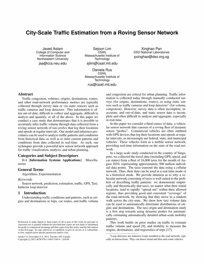
Figure 1. Distribution for Aug 1 and Aug 2 over selected 16 road segments. The x-axis includes 16 segments, one perroad. Each of these 16 segments includes 96 points, one for each 15 minute time slot during a 24 hour day. The y-axisshows the fraction of traffic at that location and time. The two curves are not well matched, although we notice thatwithin every hour time slot the offsets seem consistent.
free, person on board, busy, on break). Records are loggedat interval between 30 seconds and 2 minutes, depending onnetwork connectivity. Our study also uses the the loop countdata we obtained from Land Transportation Authority (LTA)in Singapore for about 12,000 loop detectors in about 1,000intersections in Singapore for the same period of time, Au-gust 2010. Each loop detector record gives the number ofcars that pass over each loop detector during a 15-minutetime slot. There are 2,688 time-slots for the first four weeksof August 2010. We used these time slots for our studies andmap all taxi and loop detector data in these slots.
Processing the taxi data to get the taxi counts for the cor-responding time windows for the loop detector data requiredseveral steps. First, the data is mapped to a time series ofGPS points for each car. Next, we match the time series ofGPS points to a sequence of road segments in the road net-work of Singapore. To overcome the noise and sparsity ofthe taxi GPS data, we used a map matching method based onthe Viterbi algorithm [19]. Third, we count the number oftaxis on road segments where loop detectors exist. From thisprocess, we get the taxi counts for each location in the road,which is regarded as the sampled count for the probe traffic.The loop count serves as the ground truth for general traffic.Finally, we smoothed the count data by sliding averages overa sequence of time slots ordered in time3.
Figure 1 shows the taxi and loop detector count data for16 Singapore road segments we selected randomly. Note thatthe taxi distribution (in red) tends to overestimate the loopdistribution (in blue) during much of the day, and that the
3The window size of sliding averages was determined as the minimumvalue that makes the aggregate number of data points over the window is atleast 100.
overestimation varies. During the morning rush hour, the taxiand loop distribution values are nearly identical. Thus, whilethere exists a bias, this bias certainly changes throughout theday, though it appears relatively consistent across days.
2.2 Using Taxi Probes to Infer General TrafficWe employ machine learning, and in particular, a cross-
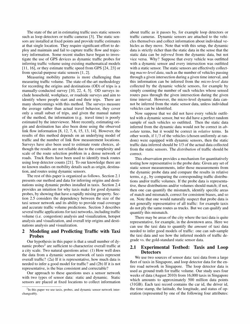
validation study, to determine the simplest corrective modelfor inferring vehicle distribution as detected by loop sensorsfrom vehicle distribution as detected by taxi sensors. Weextend this result with a cross-validation study that showsthat general traffic volume can also be inferred from the taxidata. Figure 2 shows the results of learning the correctivecoefficients for taxi data and demonstrates that taxi data canindeed be used to predict general traffic. Our analysis showsthat the best model for accurately inferring traffic distributionand volume uses (1) the hour of the day and (2) whether theday is a workday or non-workday.
Let R be the set of roads in our study. We selectedthe 1000 road segments from the Singapore road net-work whose lanes are equipped with loop detectors: R ={r1,r2, · · · ,r1000}. For road r and time slot t we normalizethe traffic value relative to the overall traffic, to determinethe fraction of traffic at that location at that time. Specif-ically, if tr and lr are the vectors representing the taxi andloop detector counts for each 15 minute time slot for road rand tr and lr are the corresponding distribution of taxis andloop detector counts4, then
tr =tr
∑1000i=1 ti
, lr =lr
∑1000i=1 li
(1)
4Since we use 4 weeks of data, the length of tr and lr is 2688.
(a) Distribution from loop detector data (blue), taxi data (yellow), and after applying the regression for taxi data (red). The probability is foundusing (1). The x-axis represents the day of the month (in this case week 4 of August 2010). Each day is further divided into 96 15-minuteintervals. The y-axis shows the distribution for each give day and 15 minute slot. The ground truth provided by loop detectors is shown in blue.The original taxi data is shown in yellow. The taxi data processed according to the learned parameters is shown in red. Notice that the redcurve is a very good match to the blue curve. The large variation between loop detector data and taxi data is removed after applying the logisticregression.
(b) Count from loop detector data (blue), taxi data (green), and after applying the regression for taxi data (red). Whereas logistic regressionwas used for regression of distributions, linear regression was naturally used for count regression. Notice the red and blue curves are wellmatched.
Figure 2. Result of regression
Our goals are (1) to examine if tr can be used to infer lrand (2) to determine how well we can predict lr from tr. Toinfer the relationship between lr and tr, we used a logisticregression model as follows:
lr =1
1+ e−(β0+β1 tr),
where β0 and β1 are the two regression parameters we learn.We find the best categorization of time slots for learning
β0 and β1 that result in the best prediction of lr, using theday-of-week and time-of-day categorization.
The intuition behind this is from the observation of thetraffic distribution pattern. We saw significant periodic pat-tern based on day and week. Specifically, our day-of-weekcategories include “Each Day of Week”, “Workday/Non-workday”, and “All Days together”, where non-workdaymeans Saturday, Sunday or holiday. Our time-of-day cat-egory varies from 15 minutes to 24 hours. For example,Workday/Non-workday as day-of-week category and 2 hoursas time-of-day category results in 2×12= 24 pairs of regres-sion parameters.
We divided the 4 weeks (Aug 01- Aug 28) data into fourone-week testing sets and four associated three-week train-ing sets. We learn the regression parameters using the train-ing set and apply the parameters to the left-out test set to findthe test error. Figure 3 shows the leave-one-out cross valida-tion training and testing RMSE errors after performing logis-tic regression for a road segment. As expected, the trainingerror decreases when we use more complex models; it de-creases as the number of time-of-day slots increase, and asthe number of day-of-week slots increase. However, the test-
ing error does not always decrease as the model complexityincreases (generally known as over-fitting). Figure 3 showsthat the best test error was achieved using Workday/Non-Workday with 15 minute slots, though substantially similarresults were achieved with slots as long as 1 hour. Figure 2(a)shows that using taxi data and the Workday/Non-workday 1hour time model we can predict the general traffic distribu-tion with high accuracy.
A similar analysis was done to infer traffic volume, repre-sented as counts, from the dynamic probes using linear re-gression. The best test error was achieved for the modelWorkday/Non-workday and 1 hour time slot, Figure 2(b),showing that using taxi data and the Workday/Non-Workday1 hour time model we can predict general traffic counts withhigh accuracy.
Let us call RMSE as absolute RMSE and define the rel-ative RMSE as the coefficient of variation of the RMSE asfollows: relative RMSE = absolute RMSE
mean of loop detector distribution . To seehow representative the taxi data is for the general traffic inSingapore, we computed the relative RMSE for all 1,000road segments and observed that the relative RMSE is lessthan 10% for vast majority (80.3%) of the road segments.
2.3 GeneralizationWhereas travel time data for each road segment can be
observed by taxis, the volume data is only available for thelocations where loop detectors exist. In this section we de-scribe how to estimate volume for every road segment. Wedevelop a computational approach to estimating the volumefor locations where the loop sensor (hence loop data) is notavailable. We estimate the traffic volume using the predictedloop count learned in Section 2.2.
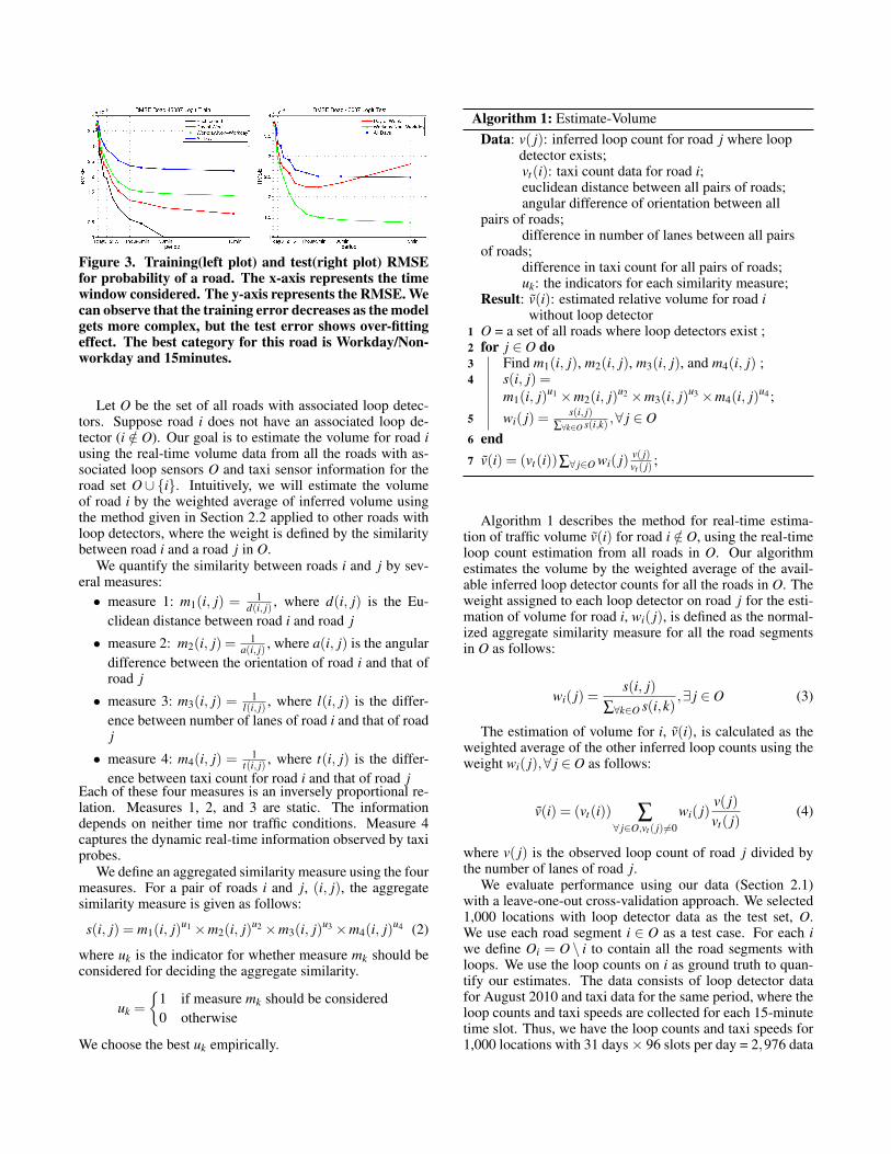
Figure 3. Training(left plot) and test(right plot) RMSEfor probability of a road. The x-axis represents the timewindow considered. The y-axis represents the RMSE. Wecan observe that the training error decreases as the modelgets more complex, but the test error shows over-fittingeffect. The best category for this road is Workday/Non-workday and 15minutes.
Let O be the set of all roads with associated loop detec-tors. Suppose road i does not have an associated loop de-tector (i /∈ O). Our goal is to estimate the volume for road iusing the real-time volume data from all the roads with as-sociated loop sensors O and taxi sensor information for theroad set O∪ {i}. Intuitively, we will estimate the volumeof road i by the weighted average of inferred volume usingthe method given in Section 2.2 applied to other roads withloop detectors, where the weight is defined by the similaritybetween road i and a road j in O.
We quantify the similarity between roads i and j by sev-eral measures:• measure 1: m1(i, j) = 1
d(i, j) , where d(i, j) is the Eu-clidean distance between road i and road j
• measure 2: m2(i, j) = 1a(i, j) , where a(i, j) is the angular
difference between the orientation of road i and that ofroad j
• measure 3: m3(i, j) = 1l(i, j) , where l(i, j) is the differ-
ence between number of lanes of road i and that of roadj
• measure 4: m4(i, j) = 1t(i, j) , where t(i, j) is the differ-
ence between taxi count for road i and that of road jEach of these four measures is an inversely proportional re-lation. Measures 1, 2, and 3 are static. The informationdepends on neither time nor traffic conditions. Measure 4captures the dynamic real-time information observed by taxiprobes.
We define an aggregated similarity measure using the fourmeasures. For a pair of roads i and j, (i, j), the aggregatesimilarity measure is given as follows:
s(i, j) = m1(i, j)u1 ×m2(i, j)u2 ×m3(i, j)u3 ×m4(i, j)u4 (2)
where uk is the indicator for whether measure mk should beconsidered for deciding the aggregate similarity.
uk =
{1 if measure mk should be considered0 otherwise
We choose the best uk empirically.
Algorithm 1: Estimate-VolumeData: v( j): inferred loop count for road j where loop
detector exists;vt(i): taxi count data for road i;euclidean distance between all pairs of roads;angular difference of orientation between all
pairs of roads;difference in number of lanes between all pairs
of roads;difference in taxi count for all pairs of roads;uk: the indicators for each similarity measure;
Result: v(i): estimated relative volume for road iwithout loop detector
1 O = a set of all roads where loop detectors exist ;2 for j ∈ O do3 Find m1(i, j), m2(i, j), m3(i, j), and m4(i, j) ;4 s(i, j) =
m1(i, j)u1 ×m2(i, j)u2 ×m3(i, j)u3 ×m4(i, j)u4 ;5 wi( j) = s(i, j)
∑∀k∈O s(i,k) ,∀ j ∈ O6 end7 v(i) = (vt(i))∑∀ j∈O wi( j) v( j)
vt ( j) ;
Algorithm 1 describes the method for real-time estima-tion of traffic volume v(i) for road i /∈ O, using the real-timeloop count estimation from all roads in O. Our algorithmestimates the volume by the weighted average of the avail-able inferred loop detector counts for all the roads in O. Theweight assigned to each loop detector on road j for the esti-mation of volume for road i, wi( j), is defined as the normal-ized aggregate similarity measure for all the road segmentsin O as follows:
wi( j) =s(i, j)
∑∀k∈O s(i,k),∃ j ∈ O (3)
The estimation of volume for i, v(i), is calculated as theweighted average of the other inferred loop counts using theweight wi( j),∀ j ∈ O as follows:
v(i) = (vt(i)) ∑∀ j∈O,vt ( j)6=0
wi( j)v( j)vt( j)
(4)
where v( j) is the observed loop count of road j divided bythe number of lanes of road j.
We evaluate performance using our data (Section 2.1)with a leave-one-out cross-validation approach. We selected1,000 locations with loop detector data as the test set, O.We use each road segment i ∈ O as a test case. For each iwe define Oi = O \ i to contain all the road segments withloops. We use the loop counts on i as ground truth to quan-tify our estimates. The data consists of loop detector datafor August 2010 and taxi data for the same period, where theloop counts and taxi speeds are collected for each 15-minutetime slot. Thus, we have the loop counts and taxi speeds for1,000 locations with 31 days× 96 slots per day = 2,976 data
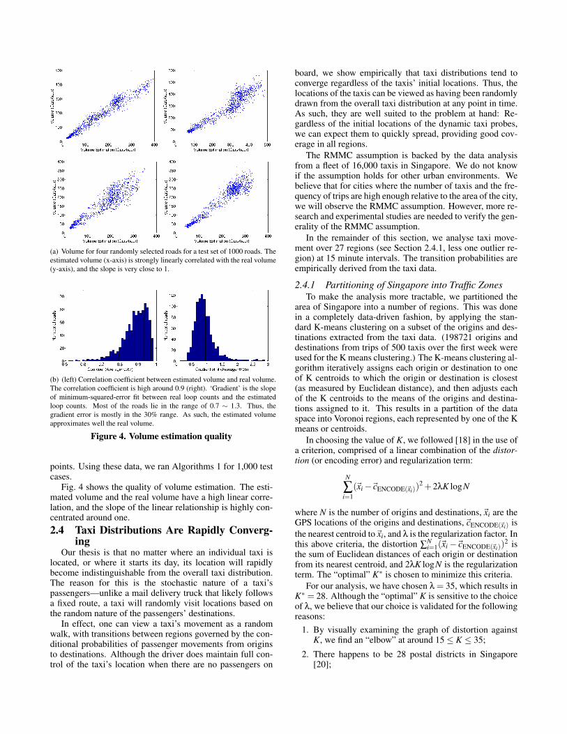
(a) Volume for four randomly selected roads for a test set of 1000 roads. Theestimated volume (x-axis) is strongly linearly correlated with the real volume(y-axis), and the slope is very close to 1.
(b) (left) Correlation coefficient between estimated volume and real volume.The correlation coefficient is high around 0.9 (right). ‘Gradient’ is the slopeof minimum-squared-error fit between real loop counts and the estimatedloop counts. Most of the roads lie in the range of 0.7 ∼ 1.3. Thus, thegradient error is mostly in the 30% range. As such, the estimated volumeapproximates well the real volume.
Figure 4. Volume estimation quality
points. Using these data, we ran Algorithms 1 for 1,000 testcases.
Fig. 4 shows the quality of volume estimation. The esti-mated volume and the real volume have a high linear corre-lation, and the slope of the linear relationship is highly con-centrated around one.2.4 Taxi Distributions Are Rapidly Converg-
ingOur thesis is that no matter where an individual taxi is
located, or where it starts its day, its location will rapidlybecome indistinguishable from the overall taxi distribution.The reason for this is the stochastic nature of a taxi’spassengers—unlike a mail delivery truck that likely followsa fixed route, a taxi will randomly visit locations based onthe random nature of the passengers’ destinations.
In effect, one can view a taxi’s movement as a randomwalk, with transitions between regions governed by the con-ditional probabilities of passenger movements from originsto destinations. Although the driver does maintain full con-trol of the taxi’s location when there are no passengers on
board, we show empirically that taxi distributions tend toconverge regardless of the taxis’ initial locations. Thus, thelocations of the taxis can be viewed as having been randomlydrawn from the overall taxi distribution at any point in time.As such, they are well suited to the problem at hand: Re-gardless of the initial locations of the dynamic taxi probes,we can expect them to quickly spread, providing good cov-erage in all regions.
The RMMC assumption is backed by the data analysisfrom a fleet of 16,000 taxis in Singapore. We do not knowif the assumption holds for other urban environments. Webelieve that for cities where the number of taxis and the fre-quency of trips are high enough relative to the area of the city,we will observe the RMMC assumption. However, more re-search and experimental studies are needed to verify the gen-erality of the RMMC assumption.
In the remainder of this section, we analyse taxi move-ment over 27 regions (see Section 2.4.1, less one outlier re-gion) at 15 minute intervals. The transition probabilities areempirically derived from the taxi data.
2.4.1 Partitioning of Singapore into Traffic ZonesTo make the analysis more tractable, we partitioned the
area of Singapore into a number of regions. This was donein a completely data-driven fashion, by applying the stan-dard K-means clustering on a subset of the origins and des-tinations extracted from the taxi data. (198721 origins anddestinations from trips of 500 taxis over the first week wereused for the K means clustering.) The K-means clustering al-gorithm iteratively assigns each origin or destination to oneof K centroids to which the origin or destination is closest(as measured by Euclidean distance), and then adjusts eachof the K centroids to the means of the origins and destina-tions assigned to it. This results in a partition of the dataspace into Voronoi regions, each represented by one of the Kmeans or centroids.
In choosing the value of K, we followed [18] in the use ofa criterion, comprised of a linear combination of the distor-tion (or encoding error) and regularization term:
N
∑i=1
(~xi−~cENCODE(~xi))2 +2λK logN
where N is the number of origins and destinations,~xi are theGPS locations of the origins and destinations,~cENCODE(~xi) isthe nearest centroid to~xi, and λ is the regularization factor. Inthis above criteria, the distortion ∑
Ni=1(~xi−~cENCODE(~xi))
2 isthe sum of Euclidean distances of each origin or destinationfrom its nearest centroid, and 2λK logN is the regularizationterm. The “optimal” K∗ is chosen to minimize this criteria.
For our analysis, we have chosen λ = 35, which results inK∗ = 28. Although the “optimal” K is sensitive to the choiceof λ, we believe that our choice is validated for the followingreasons:
1. By visually examining the graph of distortion againstK, we find an “elbow” at around 15≤ K ≤ 35;
2. There happens to be 28 postal districts in Singapore[20];
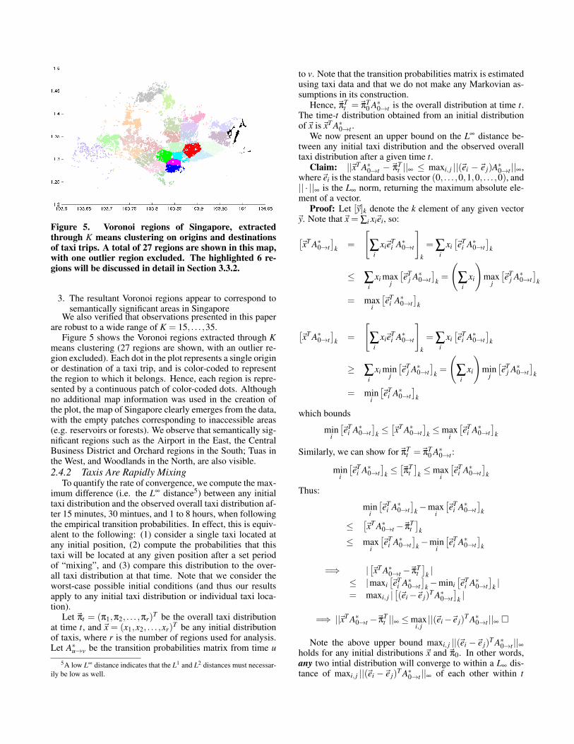
Figure 5. Voronoi regions of Singapore, extractedthrough K means clustering on origins and destinationsof taxi trips. A total of 27 regions are shown in this map,with one outlier region excluded. The highlighted 6 re-gions will be discussed in detail in Section 3.3.2.
3. The resultant Voronoi regions appear to correspond tosemantically significant areas in Singapore
We also verified that observations presented in this paperare robust to a wide range of K = 15, . . . ,35.
Figure 5 shows the Voronoi regions extracted through Kmeans clustering (27 regions are shown, with an outlier re-gion excluded). Each dot in the plot represents a single originor destination of a taxi trip, and is color-coded to representthe region to which it belongs. Hence, each region is repre-sented by a continuous patch of color-coded dots. Althoughno additional map information was used in the creation ofthe plot, the map of Singapore clearly emerges from the data,with the empty patches corresponding to inaccessible areas(e.g. reservoirs or forests). We observe that semantically sig-nificant regions such as the Airport in the East, the CentralBusiness District and Orchard regions in the South; Tuas inthe West, and Woodlands in the North, are also visible.2.4.2 Taxis Are Rapidly Mixing
To quantify the rate of convergence, we compute the max-imum difference (i.e. the L∞ distance5) between any initialtaxi distribution and the observed overall taxi distribution af-ter 15 minutes, 30 mintues, and 1 to 8 hours, when followingthe empirical transition probabilities. In effect, this is equiv-alent to the following: (1) consider a single taxi located atany initial position, (2) compute the probabilities that thistaxi will be located at any given position after a set periodof “mixing”, and (3) compare this distribution to the over-all taxi distribution at that time. Note that we consider theworst-case possible initial conditions (and thus our resultsapply to any initial taxi distribution or individual taxi loca-tion).
Let ~πt = (π1,π2, . . . ,πr)T be the overall taxi distribution
at time t, and ~x = (x1,x2, . . . ,xr)T be any initial distribution
of taxis, where r is the number of regions used for analysis.Let A∗u→v be the transition probabilities matrix from time u
5A low L∞ distance indicates that the L1 and L2 distances must necessar-ily be low as well.
to v. Note that the transition probabilities matrix is estimatedusing taxi data and that we do not make any Markovian as-sumptions in its construction.
Hence,~πTt =~πT
0 A∗0→t is the overall distribution at time t.The time-t distribution obtained from an initial distributionof~x is~xT A∗0→t .
We now present an upper bound on the L∞ distance be-tween any initial taxi distribution and the observed overalltaxi distribution after a given time t.
Claim: ||~xT A∗0→t −~πTt ||∞ ≤ maxi, j ||(~ei −~e j)A∗0→t ||∞,
where~ei is the standard basis vector (0, . . . ,0,1,0, . . . ,0), and|| · ||∞ is the L∞ norm, returning the maximum absolute ele-ment of a vector.
Proof: Let [~y]k denote the k element of any given vector~y. Note that~x = ∑i xi~ei, so:
[~xT A∗0→t
]k =
[∑
ixi~eT
i A∗0→t
]k
= ∑i
xi[~eT
i A∗0→t]
k
≤ ∑i
xi maxj
[~eT
j A∗0→t]
k =
(∑
ixi
)max
j
[~eT
j A∗0→t]
k
= maxi
[~eT
i A∗0→t]
k
[~xT A∗0→t
]k =
[∑
ixi~eT
i A∗0→t
]k
= ∑i
xi[~eT
i A∗0→t]
k
≥ ∑i
xi minj
[~eT
j A∗0→t]
k =
(∑
ixi
)min
j
[~eT
j A∗0→t]
k
= mini
[~eT
i A∗0→t]
k
which bounds
mini
[~eT
i A∗0→t]
k ≤[~xT A∗0→t
]k ≤max
i
[~eT
i A∗0→t]
k
Similarly, we can show for~πTt =~πT
0 A∗0→t :
mini
[~eT
i A∗0→t]
k ≤[~πT
t]
k ≤maxi
[~eT
i A∗0→t]
k
Thus:
mini
[~eT
i A∗0→t]
k−maxi
[~eT
i A∗0→t]
k
≤[~xT A∗0→t −~πT
t]
k
≤ maxi
[~eT
i A∗0→t]
k−mini
[~eT
i A∗0→t]
k
=⇒ |[~xT A∗0→t −~πT
t]
k |≤ |maxi
[~eT
i A∗0→t]
k−mini[~eT
i A∗0→t]
k |= maxi, j |
[(~ei−~e j)
T A∗0→t]
k |
=⇒ ||~xT A∗0→t −~πTt ||∞ ≤max
i, j||(~ei−~e j)
T A∗0→t ||∞ �
Note the above upper bound maxi, j ||(~ei −~e j)T A∗0→t ||∞
holds for any initial distributions ~x and ~π0. In other words,any two intial distribution will converge to within a L∞ dis-tance of maxi, j ||(~ei −~e j)
T A∗0→t ||∞ of each other within t
time-steps. Hence, to show that the taxi distributions con-verge regardless of initial locations, we need to show thatthis upper bound decreases quickly as t increases.
This upper bound has a very natural interpretation. Thedistribution ~eT
i A∗0→t is obtained when a subset of taxis con-centrated in a single region is tracked for t time-steps. Thisinitial configuration is arguably the worst case scenario,which we intuitively expect to take the longest time to con-verge. The upper bound is thus a measure of the worst casescenario, where two extreme initial distributions are allowedto converge over t time-steps.
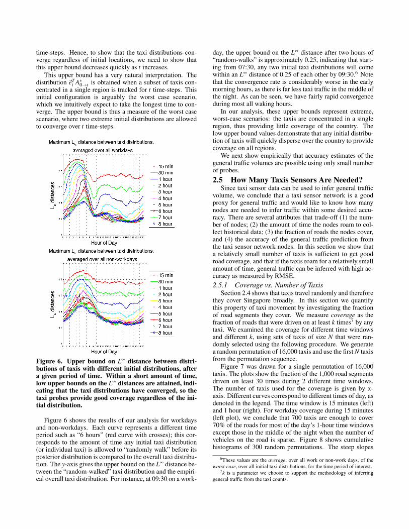
Figure 6. Upper bound on L∞ distance between distri-butions of taxis with different initial distributions, aftera given period of time. Within a short amount of time,low upper bounds on the L∞ distances are attained, indi-cating that the taxi distributions have converged, so thetaxi probes provide good coverage regardless of the ini-tial distribution.
Figure 6 shows the results of our analysis for workdaysand non-workdays. Each curve represents a different timeperiod such as “6 hours” (red curve with crosses); this cor-responds to the amount of time any initial taxi distribution(or individual taxi) is allowed to “randomly walk” before itsposterior distribution is compared to the overall taxi distribu-tion. The y-axis gives the upper bound on the L∞ distance be-tween the “random-walked” taxi distribution and the empiri-cal overall taxi distribution. For instance, at 09:30 on a work-
day, the upper bound on the L∞ distance after two hours of“random-walks” is approximately 0.25, indicating that start-ing from 07:30, any two initial taxi distributions will comewithin an L∞ distance of 0.25 of each other by 09:30.6 Notethat the convergence rate is considerably worse in the earlymorning hours, as there is far less taxi traffic in the middle ofthe night. As can be seen, we have fairly rapid convergenceduring most all waking hours.
In our analysis, these upper bounds represent extreme,worst-case scenarios: the taxis are concentrated in a singleregion, thus providing little coverage of the country. Thelow upper bound values demonstrate that any initial distribu-tion of taxis will quickly disperse over the country to providecoverage on all regions.
We next show empirically that accuracy estimates of thegeneral traffic volumes are possible using only small numberof probes.
2.5 How Many Taxis Sensors Are Needed?Since taxi sensor data can be used to infer general traffic
volume, we conclude that a taxi sensor network is a goodproxy for general traffic and would like to know how manynodes are needed to infer traffic within some desired accu-racy. There are several attributes that trade-off (1) the num-ber of nodes; (2) the amount of time the nodes roam to col-lect historical data; (3) the fraction of roads the nodes cover,and (4) the accuracy of the general traffic prediction fromthe taxi sensor network nodes. In this section we show thata relatively small number of taxis is sufficient to get goodroad coverage, and that if the taxis roam for a relatively smallamount of time, general traffic can be inferred with high ac-curacy as measured by RMSE.2.5.1 Coverage vs. Number of Taxis
Section 2.4 shows that taxis travel randomly and thereforethey cover Singapore broadly. In this section we quantifythis property of taxi movement by investigating the fractionof road segments they cover. We measure coverage as thefraction of roads that were driven on at least k times7 by anytaxi. We examined the coverage for different time windowsand different k, using sets of taxis of size N that were ran-domly selected using the following procedure. We generatea random permutation of 16,000 taxis and use the first N taxisfrom the permutation sequence.
Figure 7 was drawn for a single permutation of 16,000taxis. The plots show the fraction of the 1,000 road segmentsdriven on least 30 times during 2 different time windows.The number of taxis used for the coverage is given by x-axis. Different curves correspond to different times of day, asdenoted in the legend. The time window is 15 minutes (left)and 1 hour (right). For workday coverage during 15 minutes(left plot), we conclude that 700 taxis are enough to cover70% of the roads for most of the day’s 1-hour time windowsexcept those in the middle of the night when the number ofvehicles on the road is sparse. Figure 8 shows cumulativehistograms of 300 random permutations. The steep slopes
6These values are the average, over all work or non-work days, of theworst-case, over all initial taxi distributions, for the time period of interest.
7k is a parameter we choose to support the methodology of inferringgeneral traffic from the taxi counts.
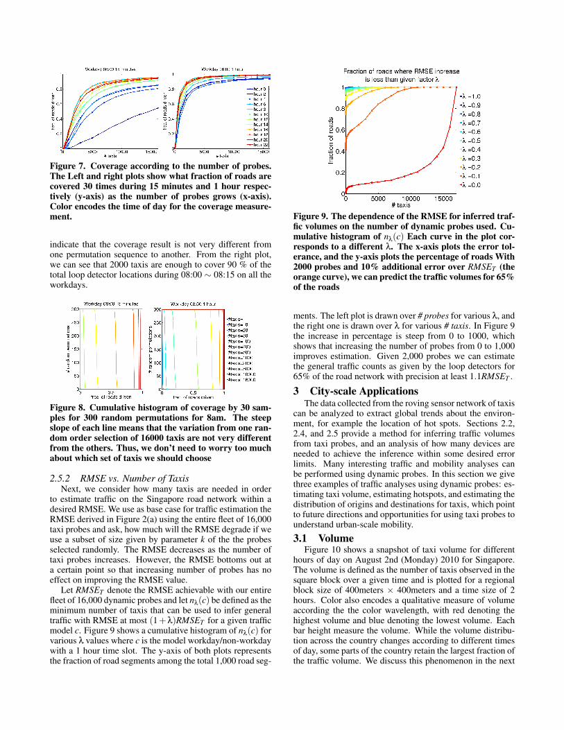
Figure 7. Coverage according to the number of probes.The Left and right plots show what fraction of roads arecovered 30 times during 15 minutes and 1 hour respec-tively (y-axis) as the number of probes grows (x-axis).Color encodes the time of day for the coverage measure-ment.
indicate that the coverage result is not very different fromone permutation sequence to another. From the right plot,we can see that 2000 taxis are enough to cover 90 % of thetotal loop detector locations during 08:00 ∼ 08:15 on all theworkdays.
Figure 8. Cumulative histogram of coverage by 30 sam-ples for 300 random permutations for 8am. The steepslope of each line means that the variation from one ran-dom order selection of 16000 taxis are not very differentfrom the others. Thus, we don’t need to worry too muchabout which set of taxis we should choose
2.5.2 RMSE vs. Number of TaxisNext, we consider how many taxis are needed in order
to estimate traffic on the Singapore road network within adesired RMSE. We use as base case for traffic estimation theRMSE derived in Figure 2(a) using the entire fleet of 16,000taxi probes and ask, how much will the RMSE degrade if weuse a subset of size given by parameter k of the the probesselected randomly. The RMSE decreases as the number oftaxi probes increases. However, the RMSE bottoms out ata certain point so that increasing number of probes has noeffect on improving the RMSE value.
Let RMSET denote the RMSE achievable with our entirefleet of 16,000 dynamic probes and let nλ(c) be defined as theminimum number of taxis that can be used to infer generaltraffic with RMSE at most (1+λ)RMSET for a given trafficmodel c. Figure 9 shows a cumulative histogram of nλ(c) forvarious λ values where c is the model workday/non-workdaywith a 1 hour time slot. The y-axis of both plots representsthe fraction of road segments among the total 1,000 road seg-
Figure 9. The dependence of the RMSE for inferred traf-fic volumes on the number of dynamic probes used. Cu-mulative histogram of nλ(c) Each curve in the plot cor-responds to a different λ. The x-axis plots the error tol-erance, and the y-axis plots the percentage of roads With2000 probes and 10% additional error over RMSET (theorange curve), we can predict the traffic volumes for 65%of the roads
ments. The left plot is drawn over # probes for various λ, andthe right one is drawn over λ for various # taxis. In Figure 9the increase in percentage is steep from 0 to 1000, whichshows that increasing the number of probes from 0 to 1,000improves estimation. Given 2,000 probes we can estimatethe general traffic counts as given by the loop detectors for65% of the road network with precision at least 1.1RMSET .
3 City-scale ApplicationsThe data collected from the roving sensor network of taxis
can be analyzed to extract global trends about the environ-ment, for example the location of hot spots. Sections 2.2,2.4, and 2.5 provide a method for inferring traffic volumesfrom taxi probes, and an analysis of how many devices areneeded to achieve the inference within some desired errorlimits. Many interesting traffic and mobility analyses canbe performed using dynamic probes. In this section we givethree examples of traffic analyses using dynamic probes: es-timating taxi volume, estimating hotspots, and estimating thedistribution of origins and destinations for taxis, which pointto future directions and opportunities for using taxi probes tounderstand urban-scale mobility.
3.1 VolumeFigure 10 shows a snapshot of taxi volume for different
hours of day on August 2nd (Monday) 2010 for Singapore.The volume is defined as the number of taxis observed in thesquare block over a given time and is plotted for a regionalblock size of 400meters × 400meters and a time size of 2hours. Color also encodes a qualitative measure of volumeaccording the the color wavelength, with red denoting thehighest volume and blue denoting the lowest volume. Eachbar height measure the volume. While the volume distribu-tion across the country changes according to different timesof day, some parts of the country retain the largest fraction ofthe traffic volume. We discuss this phenomenon in the next
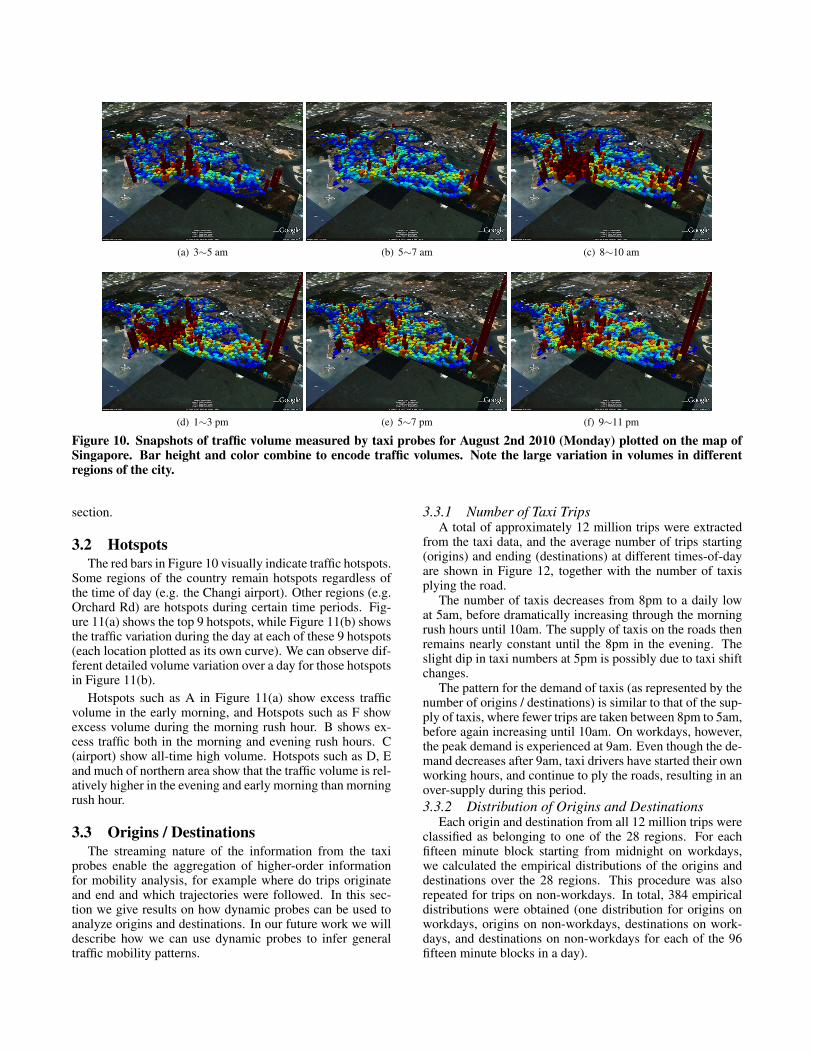
(a) 3∼5 am (b) 5∼7 am (c) 8∼10 am
(d) 1∼3 pm (e) 5∼7 pm (f) 9∼11 pm
Figure 10. Snapshots of traffic volume measured by taxi probes for August 2nd 2010 (Monday) plotted on the map ofSingapore. Bar height and color combine to encode traffic volumes. Note the large variation in volumes in differentregions of the city.
section.
3.2 HotspotsThe red bars in Figure 10 visually indicate traffic hotspots.
Some regions of the country remain hotspots regardless ofthe time of day (e.g. the Changi airport). Other regions (e.g.Orchard Rd) are hotspots during certain time periods. Fig-ure 11(a) shows the top 9 hotspots, while Figure 11(b) showsthe traffic variation during the day at each of these 9 hotspots(each location plotted as its own curve). We can observe dif-ferent detailed volume variation over a day for those hotspotsin Figure 11(b).
Hotspots such as A in Figure 11(a) show excess trafficvolume in the early morning, and Hotspots such as F showexcess volume during the morning rush hour. B shows ex-cess traffic both in the morning and evening rush hours. C(airport) show all-time high volume. Hotspots such as D, Eand much of northern area show that the traffic volume is rel-atively higher in the evening and early morning than morningrush hour.
3.3 Origins / DestinationsThe streaming nature of the information from the taxi
probes enable the aggregation of higher-order informationfor mobility analysis, for example where do trips originateand end and which trajectories were followed. In this sec-tion we give results on how dynamic probes can be used toanalyze origins and destinations. In our future work we willdescribe how we can use dynamic probes to infer generaltraffic mobility patterns.
3.3.1 Number of Taxi TripsA total of approximately 12 million trips were extracted
from the taxi data, and the average number of trips starting(origins) and ending (destinations) at different times-of-dayare shown in Figure 12, together with the number of taxisplying the road.
The number of taxis decreases from 8pm to a daily lowat 5am, before dramatically increasing through the morningrush hours until 10am. The supply of taxis on the roads thenremains nearly constant until the 8pm in the evening. Theslight dip in taxi numbers at 5pm is possibly due to taxi shiftchanges.
The pattern for the demand of taxis (as represented by thenumber of origins / destinations) is similar to that of the sup-ply of taxis, where fewer trips are taken between 8pm to 5am,before again increasing until 10am. On workdays, however,the peak demand is experienced at 9am. Even though the de-mand decreases after 9am, taxi drivers have started their ownworking hours, and continue to ply the roads, resulting in anover-supply during this period.3.3.2 Distribution of Origins and Destinations
Each origin and destination from all 12 million trips wereclassified as belonging to one of the 28 regions. For eachfifteen minute block starting from midnight on workdays,we calculated the empirical distributions of the origins anddestinations over the 28 regions. This procedure was alsorepeated for trips on non-workdays. In total, 384 empiricaldistributions were obtained (one distribution for origins onworkdays, origins on non-workdays, destinations on work-days, and destinations on non-workdays for each of the 96fifteen minute blocks in a day).
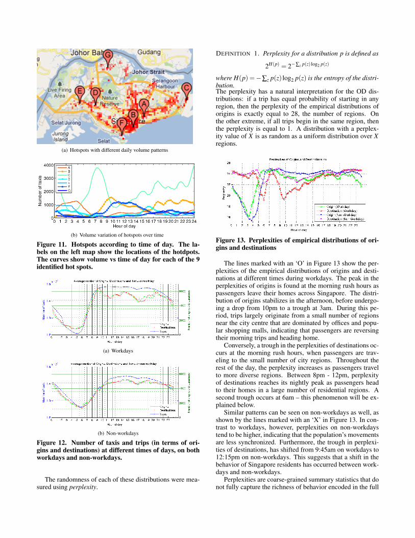
(a) Hotspots with different daily volume patterns
(b) Volume variation of hotspots over time
Figure 11. Hotspots according to time of day. The la-bels on the left map show the locations of the hotdpots.The curves show volume vs time of day for each of the 9identified hot spots.
(a) Workdays
(b) Non-workdays
Figure 12. Number of taxis and trips (in terms of ori-gins and destinations) at different times of days, on bothworkdays and non-workdays.
The randomness of each of these distributions were mea-sured using perplexity.
DEFINITION 1. Perplexity for a distribution p is defined as
2H(p) = 2−∑z p(z) log2 p(z)
where H(p) =−∑z p(z) log2 p(z) is the entropy of the distri-bution.The perplexity has a natural interpretation for the OD dis-tributions: if a trip has equal probability of starting in anyregion, then the perplexity of the empirical distributions oforigins is exactly equal to 28, the number of regions. Onthe other extreme, if all trips begin in the same region, thenthe perplexity is equal to 1. A distribution with a perplex-ity value of X is as random as a uniform distribution over Xregions.
Figure 13. Perplexities of empirical distributions of ori-gins and destinations
The lines marked with an ‘O’ in Figure 13 show the per-plexities of the empirical distributions of origins and desti-nations at different times during workdays. The peak in theperplexities of origins is found at the morning rush hours aspassengers leave their homes across Singapore. The distri-bution of origins stabilizes in the afternoon, before undergo-ing a drop from 10pm to a trough at 3am. During this pe-riod, trips largely originate from a small number of regionsnear the city centre that are dominated by offices and popu-lar shopping malls, indicating that passengers are reversingtheir morning trips and heading home.
Conversely, a trough in the perplexities of destinations oc-curs at the morning rush hours, when passengers are trav-eling to the small number of city regions. Throughout therest of the day, the perplexity increases as passengers travelto more diverse regions. Between 8pm - 12pm, perplexityof destinations reaches its nightly peak as passengers headto their homes in a large number of residential regions. Asecond trough occurs at 6am – this phenomenon will be ex-plained below.
Similar patterns can be seen on non-workdays as well, asshown by the lines marked with an ‘X’ in Figure 13. In con-trast to workdays, however, perplexities on non-workdaystend to be higher, indicating that the population’s movementsare less synchronized. Furthermore, the trough in perplexi-ties of destinations, has shifted from 9:45am on workdays to12:15pm on non-workdays. This suggests that a shift in thebehavior of Singapore residents has occurred between work-days and non-workdays.
Perplexities are coarse-grained summary statistics that donot fully capture the richness of behavior encoded in the full
distributions. To better understand the evolution of OD dis-tributions across time, we examined the probabilities of ori-gins and destinations occurring in each region.
We have highlighted 6 regions of interest for discussion,5 of which fall within or near the city center. The labelswe have used for naming the regions are purely descriptive,and do not necessarily correspond to any official naming ordemarcations. Nevertheless, a Singapore resident should beable to readily identify the regions and common activitiesassociated with them.
The 6 regions of interest (as indicated by the correspond-ing bright colors in Figure 5) are:
1. Airport (Black): The easternmost region of Singaporeholds Changi Airport, by far the most important civilian air-port.
2. Geylang (Red): Although a largely residential area,Geylang is also well- known for some of its nocturnal activ-ities.
3. Orchard (Green): Singapore’s famous shopping strip,but also houses a substantial number of offices.
4. CBD (Blue): The Central Business District is domi-nated by high-rise offices, but also caters to party-goers withits pubs and clubs.
5. Fort Canning (Magenta): Some of Singapore’s mostpopular clubs are found here. Being adjacent to Orchard andCBD, there are also shopping malls and offices in the area aswell.
6. Rochor (Cyan): At the fringes of the city area, Rochoris home to a few high-rise offices and shopping malls.
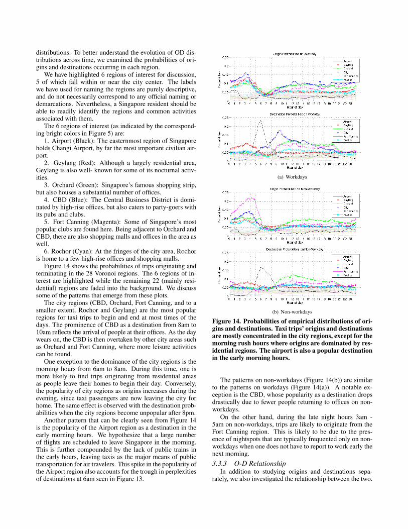
Figure 14 shows the probabilities of trips originating andterminating in the 28 Voronoi regions. The 6 regions of in-terest are highlighted while the remaining 22 (mainly resi-dential) regions are faded into the background. We discusssome of the patterns that emerge from these plots.
The city regions (CBD, Orchard, Fort Canning, and to asmaller extent, Rochor and Geylang) are the most popularregions for taxi trips to begin and end at most times of thedays. The prominence of CBD as a destination from 8am to10am reflects the arrival of people at their offices. As the daywears on, the CBD is then overtaken by other city areas suchas Orchard and Fort Canning, where more leisure activitiescan be found.
One exception to the dominance of the city regions is themorning hours from 6am to 8am. During this time, one ismore likely to find trips originating from residential areasas people leave their homes to begin their day. Conversely,the popularity of city regions as origins increases during theevening, since taxi passengers are now leaving the city forhome. The same effect is observed with the destination prob-abilities when the city regions become unpopular after 8pm.
Another pattern that can be clearly seen from Figure 14is the popularity of the Airport region as a destination in theearly morning hours. We hypothesize that a large numberof flights are scheduled to leave Singapore in the morning.This is further compounded by the lack of public trains inthe early hours, leaving taxis as the major means of publictransportation for air travelers. This spike in the popularity ofthe Airport region also accounts for the trough in perplexitiesof destinations at 6am seen in Figure 13.
(a) Workdays
(b) Non-workdays
Figure 14. Probabilities of empirical distributions of ori-gins and destinations. Taxi trips’ origins and destinationsare mostly concentrated in the city regions, except for themorning rush hours where origins are dominated by res-idential regions. The airport is also a popular destinationin the early morning hours.
The patterns on non-workdays (Figure 14(b)) are similarto the patterns on workdays (Figure 14(a)). A notable ex-ception is the CBD, whose popularity as a destination dropsdrastically due to fewer people returning to offices on non-workdays.
On the other hand, during the late night hours 3am -5am on non-workdays, trips are likely to originate from theFort Canning region. This is likely to be due to the pres-ence of nightspots that are typically frequented only on non-workdays when one does not have to report to work early thenext morning.
3.3.3 O-D RelationshipIn addition to studying origins and destinations sepa-
rately, we also investigated the relationship between the two.
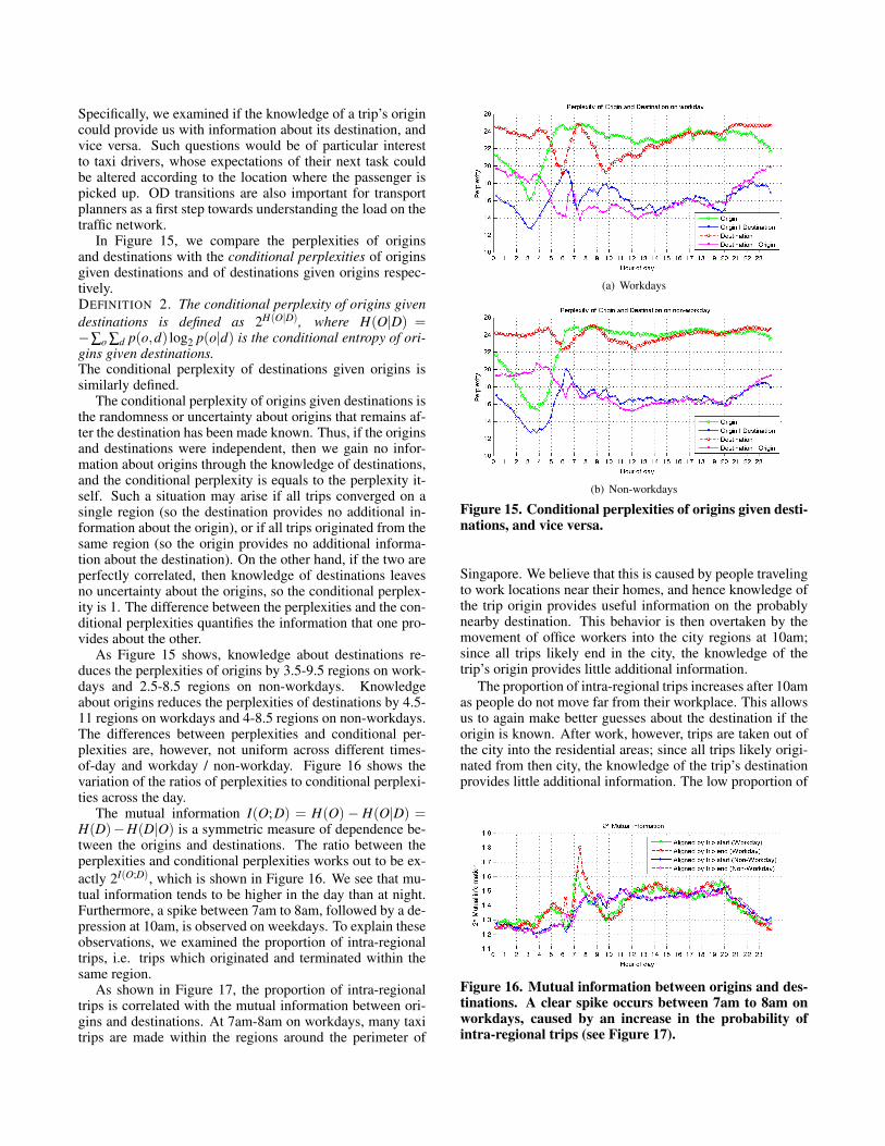
Specifically, we examined if the knowledge of a trip’s origincould provide us with information about its destination, andvice versa. Such questions would be of particular interestto taxi drivers, whose expectations of their next task couldbe altered according to the location where the passenger ispicked up. OD transitions are also important for transportplanners as a first step towards understanding the load on thetraffic network.
In Figure 15, we compare the perplexities of originsand destinations with the conditional perplexities of originsgiven destinations and of destinations given origins respec-tively.DEFINITION 2. The conditional perplexity of origins givendestinations is defined as 2H(O|D), where H(O|D) =−∑o ∑d p(o,d) log2 p(o|d) is the conditional entropy of ori-gins given destinations.The conditional perplexity of destinations given origins issimilarly defined.
The conditional perplexity of origins given destinations isthe randomness or uncertainty about origins that remains af-ter the destination has been made known. Thus, if the originsand destinations were independent, then we gain no infor-mation about origins through the knowledge of destinations,and the conditional perplexity is equals to the perplexity it-self. Such a situation may arise if all trips converged on asingle region (so the destination provides no additional in-formation about the origin), or if all trips originated from thesame region (so the origin provides no additional informa-tion about the destination). On the other hand, if the two areperfectly correlated, then knowledge of destinations leavesno uncertainty about the origins, so the conditional perplex-ity is 1. The difference between the perplexities and the con-ditional perplexities quantifies the information that one pro-vides about the other.
As Figure 15 shows, knowledge about destinations re-duces the perplexities of origins by 3.5-9.5 regions on work-days and 2.5-8.5 regions on non-workdays. Knowledgeabout origins reduces the perplexities of destinations by 4.5-11 regions on workdays and 4-8.5 regions on non-workdays.The differences between perplexities and conditional per-plexities are, however, not uniform across different times-of-day and workday / non-workday. Figure 16 shows thevariation of the ratios of perplexities to conditional perplexi-ties across the day.
The mutual information I(O;D) = H(O)− H(O|D) =H(D)−H(D|O) is a symmetric measure of dependence be-tween the origins and destinations. The ratio between theperplexities and conditional perplexities works out to be ex-actly 2I(O;D), which is shown in Figure 16. We see that mu-tual information tends to be higher in the day than at night.Furthermore, a spike between 7am to 8am, followed by a de-pression at 10am, is observed on weekdays. To explain theseobservations, we examined the proportion of intra-regionaltrips, i.e. trips which originated and terminated within thesame region.
As shown in Figure 17, the proportion of intra-regionaltrips is correlated with the mutual information between ori-gins and destinations. At 7am-8am on workdays, many taxitrips are made within the regions around the perimeter of
(a) Workdays
(b) Non-workdays
Figure 15. Conditional perplexities of origins given desti-nations, and vice versa.
Singapore. We believe that this is caused by people travelingto work locations near their homes, and hence knowledge ofthe trip origin provides useful information on the probablynearby destination. This behavior is then overtaken by themovement of office workers into the city regions at 10am;since all trips likely end in the city, the knowledge of thetrip’s origin provides little additional information.
The proportion of intra-regional trips increases after 10amas people do not move far from their workplace. This allowsus to again make better guesses about the destination if theorigin is known. After work, however, trips are taken out ofthe city into the residential areas; since all trips likely origi-nated from then city, the knowledge of the trip’s destinationprovides little additional information. The low proportion of
Figure 16. Mutual information between origins and des-tinations. A clear spike occurs between 7am to 8am onworkdays, caused by an increase in the probability ofintra-regional trips (see Figure 17).
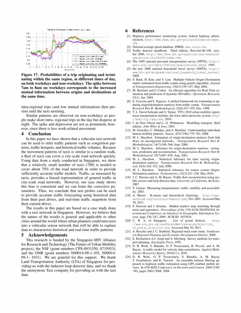
Figure 17. Probabilities of a trip originating and termi-nating within the same region, at different times of day,on both workdays and non-workdays. The spike between7am to 8am on workdays corresponds to the increasedmutual information between origins and destinations atthe same time.
intra-regional trips (and low mutual information) then per-sists until the next morning.
Similar patterns are observed on non-workdays as peo-ple make short intra- regional trips in the day but disperse atnight. The spike and depression are not as prominent, how-ever, since there is less work-related movement.4 Conclusion
In this paper we have shown that a vehicular taxi networkcan be used to infer traffic patterns such as congestion pat-terns, traffic hotspots, and historical traffic volumes. Becausethe movement patterns of taxis is similar to a random walk,a fleet of taxis can cover a city-scale road network quickly.Using data from a study conducted in Singapore, we showthat a relatively small number of taxis (700) is needed tocover about 70% of the road network in order to providesufficiently accurate traffic models. Traffic, as measured bytaxis, provides a biased representation of general traffic incity-scale road networks. However, our case study showsthis bias is consistent and we can learn the corrective pa-rameters. Thus, we conclude that taxi probes can be usedto provide accurate traffic forecasting using historical datafrom their past drives, and real-time traffic snapshots fromtheir current drives.
The results in this paper are based on a case study donewith a taxi network in Singapore. However, we believe thatthe nature of the results is general and applicable to othercities around the world where urban planners could turn taxisinto a vehicular sensor network that will be able to capturedata to characterize historical and real-time traffic patterns.5 Acknowledgements
This research is funded by the Singapore-MIT Alliancefor Research and Technology (The Future of Urban Mobilityproject), the NSF (grant numbers CPS-0931550, 0735953),and the ONR (grant numbers N00014-09-1-105, N00014-09-1- 1031). We are grateful for this support. We thankLand Transportation Authority (LTA) of Singapore for pro-viding us with the inductor loop detector data, and we thankthe anonymous Taxi company for providing us with the taxidata.
6 References[1] Highway performance monitoring system, federal highway admin-
istration, http://www.fhwa.dot.gov/policyinformation/hpms.cfm.
[2] National average speed database, INRIX, www.inrix.com.[3] Traffic detector handbook: Third edition, fhwa-hrt-06-108, octo-
ber 2006, http://www.fhwa.dot.gov/publications/research/operations/its/06108/index.cfm.
[4] The 1995 national personal transportation survey (NPTS), http://npts.ornl.gov/npts/1995/Doc/publications.shtml. 1995.
[5] the new 2000 national household travel survey (NHTS), http://www.bts.gov/programs/national_household_travel_survey/.2000.
[6] S. Baek, H. Kim, and Y. Lim. Multiple-Vehicle Origin–Destinationmatrix estimation from traffic counts using genetic algorithm. Journalof Transportation Engineering, 130(3):339–347, May 2004.
[7] M. Bierlaire and F. Crittin. An efficient algorithm for Real-Time es-timation and prediction of dynamic OD tables. Operations Research,52(1), Jan. 2004.
[8] E. Cascetta and S. Nguyen. A unified framework for estimating or up-dating origin/destination matrices from traffic counts. TransportationResearch Part B: Methodological, 22(6):437–455, Dec. 1988.
[9] T. L. David Schrank and S. Turner. TTI’s 2010 urban mobility report,texas transportation institute, the texas a&m university system, http://mobility.tamu.edu. 2010.
[10] J. de Dios Ortzar and L. G. Willumsen. Modelling transport, thirdedition. John Wiley & Sons, 2001.
[11] M. Gonzalez, C. Hidalgo, and A. Barabasi. Understanding individualhuman mobility patterns. Nature, 453(7196):779–782, 2008.
[12] M. L. Hazelton. Estimation of origin-destination matrices from linkflows on uncongested networks. Transportation Research Part B:Methodological, 34(7):549–566, Sept. 2000.
[13] M. L. Hazelton. Inference for origin-destination matrices: estima-tion, prediction and reconstruction. Transportation Research Part B:Methodological, 35(7):667–676, Aug. 2001.
[14] M. L. Hazelton. Statistical inference for time varying origin-destination matrices. Transportation Research Part B: Methodolog-ical, 42(6):542–552, July 2008.
[15] M. L. Hazelton. Statistical inference for transit system Origin-Destination matrices. Technometrics, 52(2):221–230, May 2010.
[16] J. C. Herrera and A. M. Bayen. Traffic flow reconstruction using mo-bile sensors and loop detector data. University of California, Berkeley,2007.
[17] T. Litman. Measuring transportation: traffic, mobility and accessibil-ity. 2003.
[18] A. Moore. K-means and hierarchical clustering. http://www.autonlab.org/tutorials/kmens11.pdf, Nov 2001. Accessed Mar30, 2011.
[19] P. Newson and J. Krumm. Hidden markov map matching throughnoise and sparseness. Proceedings of the 17th ACM SIGSPATIAL In-ternational Conference on Advances in Geographic Information Sys-tems, page 336–343, 2009. ACM ID: 1653818.
[20] U. R. A. of Singapore. List of postal districts. http://www.ura.gov.sg/realEstateWeb/resources/misc/list_of_postal_districts.htm. Accessed Mar 30, 2011.
[21] A. Recchia and J. C. Hadfield. Regional truck route study. Southeast-ern Regional Planning and Economic Development District, 2009.
[22] E. Richardson A.J. Ampt and A. Meyburg. Survey methods for trans-port planning. Eucalyptus Press, 1995.
[23] D. B. Work, S. Blandin, O. P. Tossavainen, B. Piccoli, and A. M.Bayen. A traffic model for velocity data assimilation. Applied Math-ematics Research eXpress, 2010(1):1, 2010.
[24] D. B. Work, O. P. Tossavainen, S. Blandin, A. M. Bayen,T. Iwuchukwu, and K. Tracton. An ensemble kalman filtering ap-proach to highway traffic estimation using GPS enabled mobile de-vices. In 47th IEEE Conference on Decision and Control, 2008 (CDC’08), pages 5062–5068, 2008.