Embed Size (px)
Citation preview
working paperCiviC PartiCiPation and Government SPendinG
By Thomas Stratmann and Gabriel Okolski
no. 10-24may 2010
The ideas presented in this research are the authors’ and do not represent official positions of the Mercatus Center at George Mason University.
Civic Participation and Government Spending
Thomas Stratmann
Gabriel Okolski
Abstract
One rationale for government spending is the provision of public goods and services, mitigating
externalities, and correcting other market failures. But government spending is often driven by
other factors, such as interest group pressure, voters’ desires for income redistribution, and
bureaucratic budget padding. This paper starts by outlining theories and research explaining
government spending and government growth. We then examine two factors that may influence
government spending: voter turnout and political contributions. While these factors may indicate
the level of citizen information and participation in the political process, they may also represent
citizens’ rent-seeking efforts to have government expenditures funneled to them. Analyzing data
from the U.S. states between 1980 and 2008, we find that voter turnout and political
contributions are positively correlated with government spending. This suggests that
government size is driven by more than the desire to provide public goods and services and to
correct for market failures.
1
I. Introduction
Economic theory suggests that the role of government is to spend resources to provide
public goods and services that would be unprovided or underprovided by the private sector and
to fix other market failures. Furthermore, Hayek (1944) suggested that one function of
government is to provide a safety net. While, in theory, these rationales should be behind
government spending, in practice, a number of alternative factors drive spending and the growth
in government spending. These include citizen demand for government spending, fiscal illusion,
institutional arrangements, and interest-group pressure (see, for example, Rodrik 1998, Besley &
Case 2003, Rice 1986). These explanations provide alternative rationales for government
spending; in many cases, these drivers may lead to outcomes that concentrate benefits on certain
groups while reducing total economic welfare.
This paper will review the economics and, more specifically, public choice literature to
evaluate some of these theories that explain government spending. Using state panel data from
1980–2008, this paper builds on the literature to empirically test the effect of citizen participation
in the political process, measured by voter turnout and the effect of campaign contributions by
individuals on state government spending. While individual political contributions and voter
turnout are a measure of participation in the political process, they are also indicators of potential
rent-seeking efforts or changes in the voting pool that could lead to redistributive policies. The
paper will also discuss the implications that these results, controlling for other factors, have on
government spending.
Our analysis of the effects of political engagement on government expenditures adds to
an extensive and well-established literature on the drivers of government spending. While past
work has discussed the effects of economic, geographic, and institutional factors, to the best of

2
our knowledge, previous research has not studied the effects of both political contributions and
voting activity on government size. This paper thus contributes to the literature by analyzing how
civic participation, evidenced by voting, contributions, and the interaction of the two, influences
government spending.
II. Review of Traditional Theories and Alternate Rationales for Government Spending
From a traditional theoretical perspective, government spending is justified as a method
to bolster economic growth when the state uses taxpayer funds to provide welfare-enhancing
public goods and services, such as military defense, enforcement of contracts, and police
(Wagner 2007, 28). Hayek (1944) also made the case that there is a rationale for government to
provide its citizens with a sort of safety net. Because of non-excludability and non-rivalry in
consumption, private entities have insufficient incentives to provide these goods and services. As
such, an omniscient government can enhance total economic welfare by redirecting resources to
uses that are beneficial to citizens once implemented, but would not otherwise be provided to
individuals. Though these functions often require regulation or legislation instead of spending,
government should theoretically act to eliminate certain other market failures and externalities.
Wagner (1877) incorporates this idealistic view of the state in his explanation for the
growth in government spending. In what has become known as Wagner’s Law, he theorized that
growth in industrial progress and economic growth in a nation will necessarily be accompanied
by an increased share of public expenditure relative to economic output. This theory, which
predicts that the income elasticity of demand for public goods is greater than unity, underlies the
notion that government spending is aimed at providing public goods and eliminating
externalities; the citizens of a more industrialized society are likely to have more income and
3
thus ought to have higher demand for public goods and services. Wagner’s law does not appear
to have broad support in the literature, however. Larkey et al. (1981) summarize results from
testing this theory. They point out that 20th-century studies of Wagner’s law yield generally
weak confirmation of some version of Wagner’s law, although some scholars find no support for
Wagner’s proposition.
In addition to Wagner’s law, scholars have tested other “benevolent” theories that explain
government growth, such as the government as provider of insurance. For example, in looking at
data from 97 countries, Rodrik (1998) found evidence that higher levels of government spending
provide insurance to citizens in open economies who are vulnerable to trade shocks.
Research in public choice and government spending has tested theories related to a
government not interested in spending on welfare-enhancing goods and services, but related to a
government seeking to accomplish other ends. These competing explanations provide some
alternative rationale for why governments spend money and why government spending may be
increasing. Rather than serving to provide public goods and mitigate externalities, spending may
instead be driven by voters’ ability and desire to redistribute wealth, the pressure of interest
groups, the budget-maximizing incentives of bureaucratic agencies, or government’s incentive to
deceive citizens about its true size.
Meltzer and Richard (1983) test the theory that government serves largely to redistribute
income from the upper to the lower part of the income distribution. They hypothesize that the
greater demand for redistribution, the lower the median voter’s income is relative to the mean
income of all voters. Using U.S. data from 1938–1976, the researchers find evidence that a lower
income of the median voter (relative to the mean) leads to higher government spending and
4
thereby redistribution.1 Thus, instead of arising out of increased demand for government goods
and services, larger government may come about to facilitate this redistribution. Voter ideology,
instead of economic realities, may also serve as a driver of spending. Cusak (1997) studies 16
OECD countries and finds that left-of-center governments tended to favor more redistribution
and government spending between 1955 and 1989.
In addition to voters driving the size of government, there is some evidence that other
actors such as interest groups contribute to government size. In theory, these groups can organize
voters to influence policymakers and pressure them into instituting policies that are not socially
optimal (Mueller, 520–521). For example, Rice (1986) presents evidence that labor union and
interest-group efforts to introduce policies that reduce economic hardship contributed to the
growth in government in Europe between 1950 and 1980. Mueller and Murrell (1985, 1986) also
show empirical evidence that political parties supply interest groups with favors in exchange for
support, suggesting a rent-seeking arrangement. They find that the number of interest groups in a
sample of OECD countries is positively correlated with government size.
In addition to groups outside of government affecting its size, groups within government
may also have an effect. Niskanen (1971) proposed a model by which bureaucratic agencies have
an incentive to maximize their budgets above what would be demanded by a bureau’s sponsor.
These higher budgets are used to pad salaries, give more leisure time, and fund more amenities
for the agency. Thus an agency may purposely keep unproductive projects going in order to
continue to ask for larger appropriations from Congress. Miller (1981) finds evidence that city
and country bureaucrats in Los Angeles County seem to be expanding the size and scope of their
1 The median income is one which is midway between the highest and lowest incomes. This can be contrasted with
the mean which is the average of all incomes. If the median is below the mean, it suggests that there is not a large
concentration of wealth at the top which would tend to drive the mean upward. Such a concentration of wealthier
voters might spend more to reduce the influence of lower income voters seeking redistribution of wealth.
5
jurisdictions. Ferris and West (1996) find evidence that higher government spending can be
attributed largely to slower productivity growth in government relative to other industries. This
slower productivity is likely a function of bureaucracies employing more resources than
necessary in order to ensure an expansion, rather than a contraction, of budgets. The finding is
also consistent with Baumol’s cost disease argument, by which productivity tends to stagnate in
the service sector since providing services is labor intensive.
Bureaucratic agencies are not the only government entities with an incentive to increase
government size. Voters ultimately have an incentive to remain rationally ignorant about
government when information costs are high and outweigh the marginal benefit that a citizen
obtains from being well informed about a potential policy outcome. Thus, the legislature may
create a more complicated tax and funding system than necessary to obscure the true cost of
government, thereby creating a fiscal illusion. While some researches have found experimental
proof of the effectiveness of fiscal illusion (Tyran and Sausgruber 2000), the theory has not
found widespread empirical support in the literature.
Some scholars also examine how institutional factors affect spending. Barro (1973)
created one of the earliest theoretical models showing how politician interests may diverge from
the electorate’s interests. Scholars have found that various factors that can move an official away
from providing an ideal amount of a public good include infrequent elections, increased political
salary, and a governor who is unable or unwilling to seek reelection after her current term. A
number of researchers have evaluated the effect of various institutional arrangements on
spending. For example, List and Sturm (2006) find that in “green” states, environmental
spending is lower when the governor is facing a binding term limit. Besley and Case (2003)
6
provide a comprehensive discussion of empirical evidence for the relationship between electoral
institutions and political outcomes.
The recent literature also examines the importance of voter information and elections on
government size. Rogers & Rogers (2000), for example, theorize that tighter elections lead to an
increased likelihood of candidates pursuing a strategy of tax cuts. Using state data, they find that
lower margins of victory in gubernatorial elections are correlated with lower levels of
government expenditure.
Besley and Burgess (2002) evaluate whether variables for economic performance,
political institutions, and voter information have an effect on government responsiveness. Using
data from India they find that public food distribution and relief expenditure are greater where
governments face greater electoral accountability and where newspaper circulation is highest.
Stromberg (2004) evaluates the effects of a New Deal program that increased radio use in
households. He finds evidence that the expansion of radio to certain rural areas led to increased
government transfer spending in these areas. This finding indicates that increased electoral
information and participation may lead to larger budgets because of citizens’ ability to attract
additional spending.
III. Conceptual Framework
From a theoretical standpoint, voter participation, either in terms of turnout or in terms of
contributing to political campaigns, can have ambiguous effects on government size. The amount
of individual political contributions is a measure of civic activity and political awareness in a
given state, traits that may be associated with greater citizen understanding of the budgetary
process, tax structure, and other fiscal indicators. In such a way, voters may be able to better hold
7
elected officials accountable for budgets that contain spending above or below the median
voter’s preferred point and may be able to better prevent politicians from increasing spending
through a political budget cycle, as modeled by Rogoff (1990).
On the other hand, high levels of contributions can indicate that more individuals are
involved in a rent-seeking contest (in a manner similar to that described by Tullock, 1980) to
gain transfers from office holders. Liebman and Reynolds (2006) find that political contributions
from firms are effective in affecting congressional decision-making and that higher contribution
levels attract higher level of rewards. Higher individual contributions may indicate increased
efforts by voters in a given state to rent seek and attract additional government services and
transfer spending. In a similar manner to that described in Stromberg’s (2004) evidence of the
connection between radio penetration and federal grants, more informed voters may be able to
attract additional spending.
A number of studies in the literature have found that positive correlation between wealth
and political contributions (see, for e.g., Joulfaian & Marlow 1991). Since high-income
individuals are more likely to contribute to political campaigns than low-income individuals,
observing an increased number of political contributions likely means that, ceteris paribus, there
are a larger number of high-income earners participating in the political process. Given high
levels of contributions, then, one may be likely to see lower levels of government redistributive
spending because high-income voters are less likely to favor income redistribution to lower-
income earners. But because increased levels of money in politics may also be indicative of high-
income earners’ attempts to garner rents, leading to more government spending, the net effect of
campaign contributions on government size is ambiguous.
8
In this paper we hypothesize that turnout leads to an increase in government size because
we assume that larger turnout implies that more lower-income voters are included in the voting
pool (Lijphart 1997). There is empirical support for the assumption that the upper income classes
have higher participation rates than the lower income classes. Countless studies using survey
data within countries have found a positive correlation between participation and various
measures of economic status like education and income (Powell (1980), Verba and Nie (1972),
Verba, Nie and Kim (1978)). Although both variables are usually positively related to
participation rates, the impact of income sometimes disappears once education is controlled for
and Chapman and Palda (1983) even obtained a negative and significant coefficient on income in
an equation to explain voting, once education was included. One explanation for the strong
association between education and voting is that better-educated people gather more information
about government policies and candidates in the course of their work and leisure-time activities.
Thus, the costs of becoming informed and voting are lower for better-educated citizens (Filer,
Kenny, and Morton, 1993).
Thus, applying the model of Meltzer and Richard (1983), having more low-income voters
in the voting pool increases government spending due to increased demand for redistribution.
This is because low-income earners support spending policies that channel resources from
wealthier groups to them in the form of direct transfers or government-provided goods and
services. Mueller and Stratmann (2003) find empirical support for this hypothesis. They find
cross-national evidence that higher voter turnout leads to larger government expenditures.
9
IV. Empirical Model and Data
We use state level data to test the effect of civic participation on government size. The
dependent variable is a state’s spending as a percentage of its GDP. Independent variables
include individual political contributions and voter turnout. Individual political contributions are
the statewide sum of individual contributions to a candidate or other political committee in the
year of an election and the year prior; these committees include political action committees,
party committees, campaign committees for presidential, U.S. House, and U.S. Senate
candidates. We collected these data from the Federal Election Commission website, which
provides detailed contribution data to the public. We measure voter turnout as the percent of
eligible voters casting a ballot in a federal general elections. We also include an interaction term2
for turnout and contributions to evaluate the combined effects of these two factors on
government spending.
The empirical model we use incorporates controls similar to those in Besley and Case
(1995): state income per capita, population, the proportion of state residents younger than 18
years of age, and the proportion of state residents 65 years of age and older. We also include in
the regression a variable measuring enrollment in universities within the state divided by state
population as an indicator of statewide education levels. Also, we include state and year fixed
effects. The empirical model is:
Govit = β0 + β1Contributionsit + β2Turnoutit + β3Turnoutit*Contributionsit + β3Xit + γi + µt + εit
2 An interaction term is the product of two variables. Here, it is the product of turnout and contributions.
10
where the X vector includes the aforementioned control variables. The unit of observations is
state i in year t. We employ two measures of government size: “Gov” government spending as a
percent of state product and per capita government spending.
The data cover all 50 states for all even-numbered years from 1980 to 2008. We consider
even-numbered years because they are coincident with federal elections. The dataset includes
749 observations; one observation (Louisiana in 1982) has been omitted due to missing turnout
data. Our contribution variable is the sum of individual contributions to a candidate or political
committee for a given state for the two-year election cycle. The two-year contributions are then
divided by the state population and logged. The variable “Contributions” therefore measures the
log of the two-year contributions per capita.
While contributions may measure rent seeking or also capture the degree to which
citizens are politically active, the estimates on the contribution variable and turnout have to be
interpreted with caution. If government grows, more resources are there for redistribution,
potentially leading to more rent-seeking activity. Further, turnout may respond to government
size. Thus it may be that government size determines campaign contributions and turnout, not
vice versa. In an attempt to address this issue, we do not use contributions from state races to
measure political participation in the state, but rather individual contributions for federal
elections, which measure the extent to which individuals in the state are politically active, but are
less likely a respond to state government size as would contributions to state races. Further,
while turnout may respond to government size, it is not clear whether turnout increases or
decreases as government size grows. Mueller and Stratmann (2003) find little evidence that
turnout is endogenous in their government-size regressions. In this paper we treat turnout as
exogenous.
11
Electoral turnout data come from the United States Election Project at George Mason
University and the “Turnout” variable is the percent of a state’s voting eligible population that
participated in a given year’s election. State GDP data come from the Bureau of Economic
Analysis. All remaining data were taken from current and past copies of the Statistical Abstract
of the United States. All data denominated in dollar values have been converted into 2008
dollars.
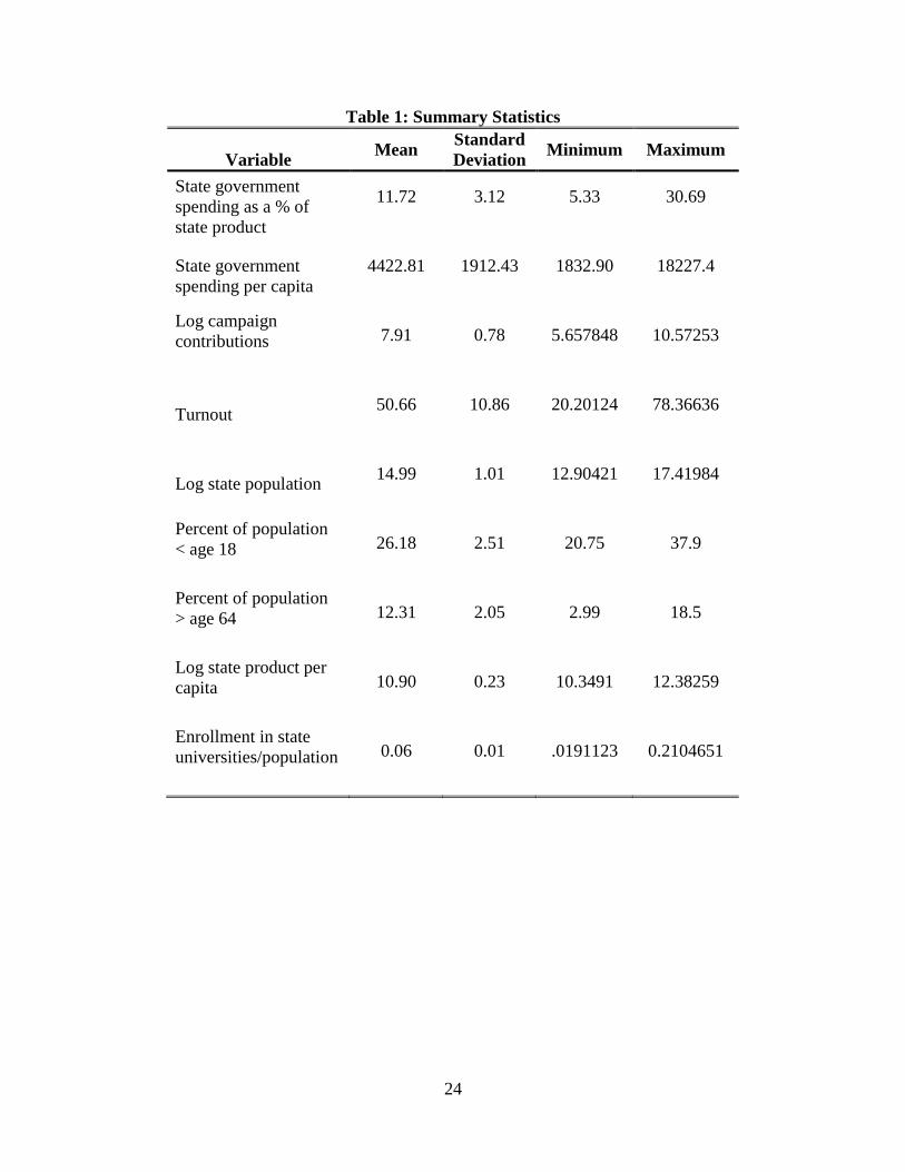
Table 1 lists the summary statistics for key variables in the regression models. The mean
turnout in the data set is 50 percent, with a minimum of 20 percent and a maximum of 78
percent. These are turnouts measured for federal elections. The mean percent of population less
than 18 years of age is 26 percent and the mean for those over 64 years of age is 12 percent.
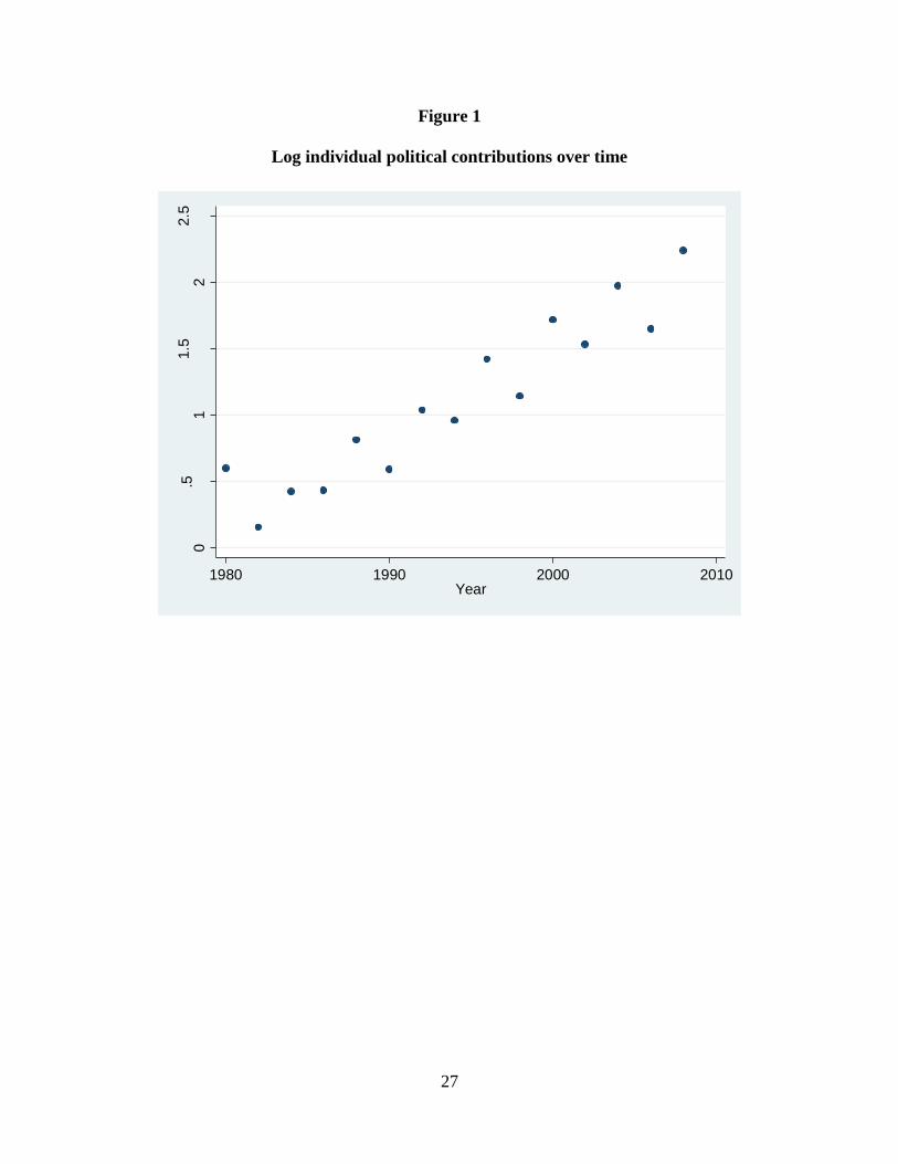
Figure 1 shows how campaign contributions have evolved since 1980. The vertical axis measures
log individual political contributions. The graph reveals a steady increase over time and that
midterm elections, relative to presidential election years, tend to lead to a dip in contributions.
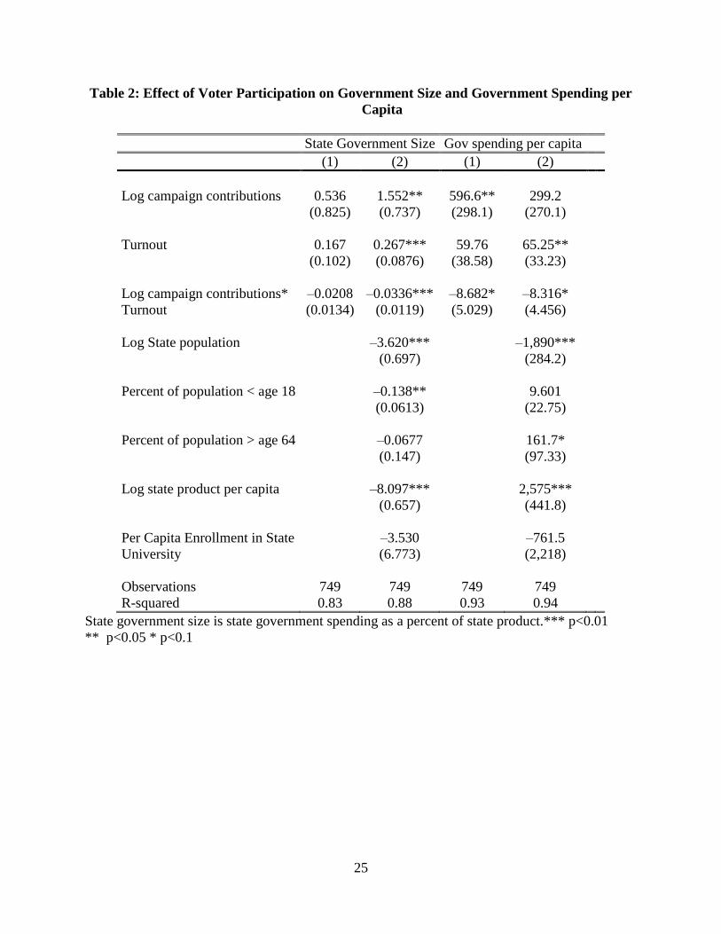
V. Results
Table 2 reports the results from the OLS regressions on both empirical models (excluding
state and year dummy variables), along with robust standard errors, statistical significance, and
the R-squared for the regressions. The dependent variable in the first two columns is state
spending as a percent of GDP per capita. The regressions in columns 1 and 2 explain a
significant amount of the variation in state spending with R-squared values of 0.833 and 0.879,
respectively. Those in columns 3 and 4 explain nearly all of the variation, with R-squared values
of 0.928 and 0.943, respectively.
12
Columns 1 and 2 in table 2 show results when the dependent variable is state government
spending as a percentage of state GDP. The coefficients for both political contributions and
turnout are positive, indicating that political contributions and voter turnout have a positive
correlation with government size and spending. Both of these variables are statistically
significant in the second regression, for which various controls are added. Additionally, the
interaction term between the two variables is negative for both regressions and statistically
significant for the second specification, indicating that when turnout is high, more political
contributions lead to less government spending.
In Table 2, columns 3 and 4, the dependent variable is state government spending per
capita. The results are similar to the regressions that have spending as a percent of state product
as the dependent variable. As in the case of state government size, campaign contributions have a
positive effect on spending; this effect is statistically significant in the baseline specification with
no additional control variables. Turnout is also positive but only significant when additional
controls are added to the model. The interaction term between campaign contributions and
turnout is negative, as was the case with the first two regressions, indicating that at higher levels
of contributions, turnout has a negative effect on spending. Nonetheless, these results are not
statistically significant at the 5 percent level.
Among the control variables, in all specifications, population is statistically significant
and negatively correlated with relative government size: this result indicates that there may be
scale effects when it comes to government spending whereby relatively large fixed costs are
required to set up basic government services in a state. In a model of country size, growth, and
trade openness, Alesina et al. (2000) indicate that larger countries have economies of scale
effects, and empirically find that government spending as a share of GDP is negatively correlated
13
with a country’s population. Besley and Case (1995), using a similar specification to our model,
similarly find a negative correlation between population and state per-capita spending indicating
support for this effect.
GDP per capita is negatively correlated with state government size and positively
correlated with spending per capita. This shows that wealthier states spend more on a per capita
bases but less as a percent of the state product. Our result for spending per capita is in line with
the results in Besley and Case (1995).
The results of the variables measuring the faction of the population under 18 and over 64
are mixed. Both demographic variables are not statistically significant in the government
spending per capita regression. In the government size regression, the coefficient on those under
ages 18 is negative and statistically significant. The negative sign on this age group is consistent
with the hypothesis that more voter participation by younger individuals leads to less spending
since younger residents do not carry the burdens of potential unemployment payments and other
government services. Conversely, a higher proportion of elderly residents would be expected to
have a positive correlation with state spending for the opposite reasons. Meltzer and Richard
(1981, 1983) propose and find empirical support for a general equilibrium model in which
increases in the proportion of the aged population receiving government assistance increases
redistribution to those groups.
While the coefficient on those over 64 years of age is positive when the dependent
variable is spending per capita, when the dependent variable is state government size, the
coefficient is negative. One potential explanation for this unexpected result is that during certain
years covered by the dataset, all states have seen increased numbers of early baby-boomers
14
become elderly. This generation may bring additional financially secure individuals into the
elderly population and this reduces the demand for government expenditures.
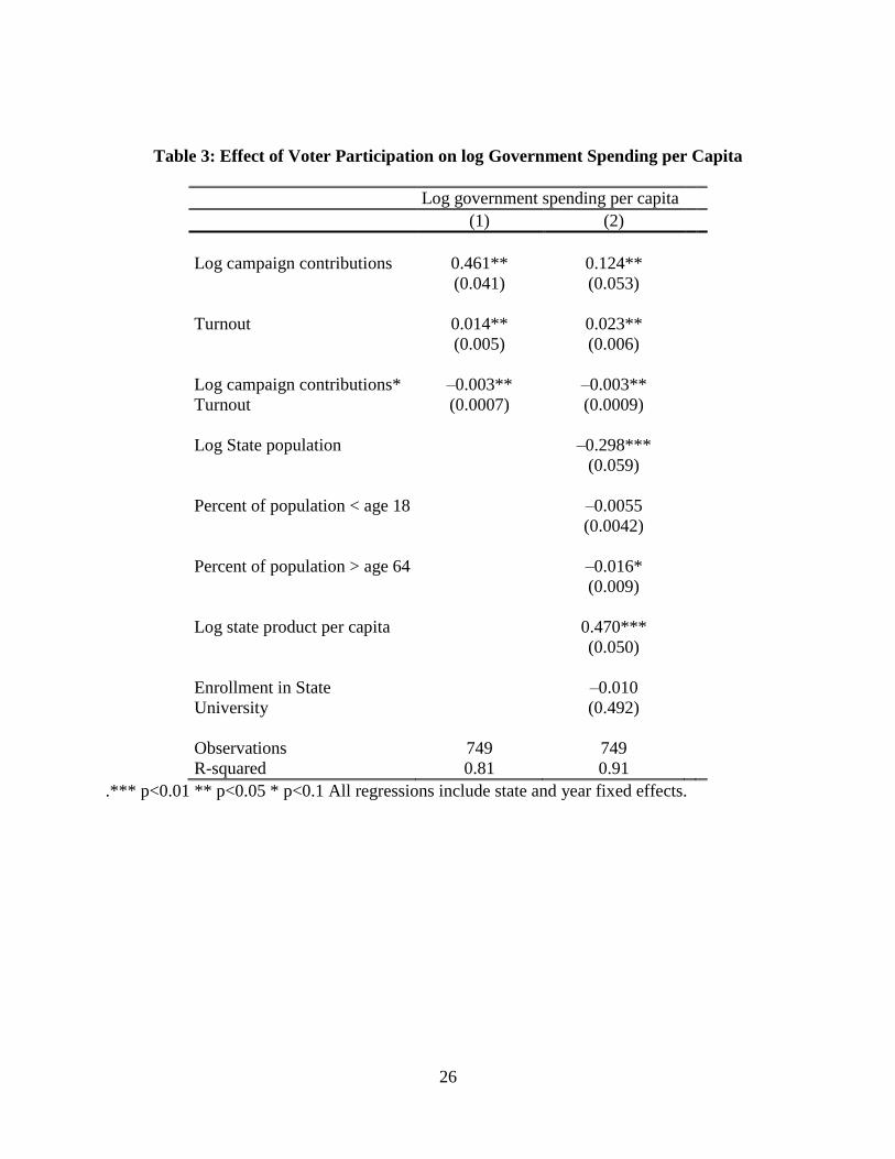
Table 3 shows the results for two alternate specifications to test the sensitivity of the
results when using the log of government spending per capita instead of the level of government
spending per capita as the dependent variable. In the literature on government size, both the level
and the log of spending per capita are commonly used. The specifications in table 3 mirror those
of table 2.
The results from this regression analysis in table 3 show that campaign contributions and
turnout have a positive and statistically significant effect for both specifications. This result is in
line with the coefficients estimated in the specifications from table 2. When government
spending per capita is logged, the signs stay the same but the point estimates have higher levels
of statistical significance. The same holds true for the turnout times log contribution interaction
term in the specifications using the log of government spending per capita: in both specifications
the coefficients on the interaction term is also negative, and in both specifications the point
estimate is statistically significant. These results provide additional evidence that turnout and
political contributions have a positive and significant effect on government size and spending,
but that higher levels of turnout result in contributions having a negative effect on state spending.
With the exception of the point estimate on the variable measuring the elderly population,
the point estimates on the control variables in table 3 have the same signs as the same signs as
the corresponding estimates in table 2. Both of our demographic variables have a negative sign
and the point estimates on the elderly is statistically significant at the 10 percent level.
The results of these models have several implications on the understanding of the effects
of citizen information and participation on the levels of government spending. First, the results
15
show that voter turnout in elections has a positive effect on government spending, and the size of
this effect increases and becomes more statistically significant when additional controls are
added to the models. This result is in line with our hypothesis and with previous findings about
the effects of turnout.
Increases in state voter turnout are correlated with increases in voting enfranchisement
(historically, giving women and minorities the right to vote) and additional participation from
voters who are on the lower end of the income scale. This effect has a number of potential
consequences. Most notably, in a manner analogous to that discussed by Meltzer & Richard
(1983), an increase in the number of voters below the median income can result in an increase in
redistribution measured as the size of government. This occurs because lower-income individuals
have incentive to seek an increase in the amount of government transfers they receive from
wealthier citizens. In addition to redistributive transfers, lower-income voters may support
expanded provision of public goods and services.
Additionally, higher levels of voting may point to rent-seeking effects that come along
with a better-informed citizenry. Indeed, higher levels of turnout, in addition to bringing in
lower-income earners, can point to a state whose population has a higher level of political
engagement or participation. These individuals may be more likely to have better familiarity with
government structure and may better understand effective lobbying methods in order to gain
their preferred types of government grants and projects. In a similar effect as that discussed by
Stromberg (2004), better-informed citizens, as indicated by higher voter turnout, may be able to
have a positive impact on government spending.
We find that political contributions have a positive correlation with state spending. This
relationship is only statistically significant in one specification with state government spending
16
as a percentage of state GDP as the dependent variable, indicating the potential for future
research to determine whether this positive link between political contributions and government
spending is conclusive. Nonetheless, the positive correlation supports the hypothesis that rent
seeking, measured as campaign contributions, is one driver of government spending. By
spending more on a candidate or political committee, a state’s voters may be engaged in a sort of
contest with other voters to obtain rents from a candidate whom they hope will be elected.
Assuming that these contributors take the same approach to state-level politics as they do to
those on a federal level, a higher level of contributions could lead to increased spending as
elected politicians distribute rents to “pay back” the contributors who got them elected.
Additionally, individuals who contribute to political causes are likely to be better
informed about the political process and current events (at least some aspects of them); someone
with poor information is likely to have lower incentives to give money to a candidate or
committee. Thus an increased level of contributions in a state may point to a better-informed
citizenry and one that is better able to obtain government grants and transfers. This argument ties
into the citizen information argument that applies to states with higher levels of turnout.
Despite the individual effects of turnout and contributions, the interaction between them
sheds some light as to how contributions can mitigate the spending effects of voter turnout. As
mentioned above, the negative coefficient on this interaction indicates that at higher levels of
turnout, contributions lead to a decline in government spending and size. For the regressions in
columns one through four in table 2, this critical level of turnout occurs at 26 percent, 46 percent,
69 percent, and 36 percent, respectively. It should be noted that three of these values are actually
below the sample mean of 51, indicating that turnout is significant enough to have this result on
contributions in a sizable number of the states and years being analyzed.

17
Likewise, at increasing levels of contributions, turnout begins to have a negative effect on
spending and government size. For the regressions in columns one through four, the critical level
of contributions are 8.0, 8.0, 6.9, and 7.9, respectively. Two of these values are at or below the
sample mean of 7.9, indicating that this effect holds for a sizable portion of observations.
As a sensitivity test we also examined the effect of political contributions as a percent of
state product on government size, instead of contributions per capita. When we do so, we find
similar results as those reported in our tables.
The most likely explanation for this phenomenon deals with the demographic connection
between political contribution and wealth. Higher levels of political contributions in a state point
to increasing numbers of wealthy participants in the political process. The inclusion of additional
higher-income voters directly counters the “income effects” of increasing turnout: a larger
number of voters no longer include only lower-income individuals who have an incentive to seek
in increase in government size. If anything, the inclusion of additional high-income voters may
lead to reduced spending because these participants would lose out from redistributive policies.
These factors point toward an explanation for some of the reasons for government
spending. Rather than government spending being used to correct market failures, mitigate
externalities, and provide public goods that are welfare-enhancing, government spending may be
the result of rent seeking and serves to redistribute income. This is increasingly the case when
lower-income voters have influence in the political process. In the case of a government that
seeks to spend based only on correcting externalities, providing public goods and secure property
rights, increased voter turnout and political contributions ought to have no influence on the
spending decisions in a state. Nonetheless, a statistically significant relationship indicates that
18
varying levels of citizen participation in rent seeking activities and increased participation of
lower-income voters can be effective in increasing spending levels.
While an increased number of contributions draws more higher-income voters into the
voting pool and causes turnout to have a lower effect on spending, it is unclear whether this
effect serves to constrain government spending in the direction to an optimal size of government,
or whether it represents a tug-of-war between two different demographic groups competing to
achieve certain policy outcomes. Ultimately, determining the ideal level of government spending
is a difficult exercise in any real-world setting. This question aside, the results in this paper show
that at a certain level of contributions, the interaction of contributions and turnout shrinks the
size of government and spending.
This is not to say that having additional political contributions always reduce government
size. They reduce government size only when turnout is sufficiently high. Not considering this
interaction effects, higher individual contributions and thus perhaps rent-seeking efforts seem to
increase government size and spending. Future research may determine the exact mechanism
through which this potential rent-seeking channel operates.
VI. Conclusions
This paper presents an analysis of data from all states in federal election years from 1980
to 2008 to evaluate the effects that political contributions and voter turnout have on the size of
state government spending. The results show that voter turnout is positively correlated with both
government spending per capita and government size relative to state product: this finding is
consistent with the hypothesis that increased turnout draws voters from the lower part of the
income distribution who are more likely to support redistributive and government spending

19
policies. Additionally, political contributions are associated with an increase in the size of
government and government spending per capita. This could speak, in part, to the success of
campaign contributions as a sort of rent seeking effort by which individuals expect to be
rewarded (in the form of government services and transfers) by candidates following their
election.
The positive relationship between government spending and turnout is not present in all
states. When political contributions rise above a certain level, political participation begins to
have a negative effect on government expenditures. This likely occurs because political
contributions tend to be positively correlated with wealth; thus, increased levels of contributions
imply a larger number of wealthier voters. The effect of these higher-income participants can end
up mitigating the lower-income voters’ desire for transfers and wealth redistribution, thus
leading to lower spending.
Overall, this paper shows that some of the growth in government spending may be
partially explained by the increased participation in politics. Furthermore, these results point to
the fact that government size and government spending is not necessarily determined only by
fixing market failures and providing public goods and services. Instead, an important explanation
for government size is the demand of those who are politically active: voters and those who
contribute to election campaigns.
20
References
Alesina, Alberto, Spolaore, Enrico, & Wacziarg, Romain. 2000. “Economic Integration and
Political Disintegration.” American Economic Review. Vol. 90, No. 5, pp. 1276–1296.
Barro, Robert J. 1973. “The Control of Politicians: An Economic Model.” Public Choice. Vol.
14, No. 1, pp. 19–42.
Besley, Timothy & Burgess, Robin. “The Political Economy of Government Responsiveness:
Theory and Evidence from India.” Quarterly Journal of Economics.Vol. 117, No. 4, pp.
1415–1451.
Besley, Timothy & Case, Anne. 1995. “Does Electoral Accountability Affect Economic Policy
Choices? Evidence from Gubernatorial Term Limits.” The Quarterly Journal of
Economics. Vol. 110, No. 3 (1995), pp. 769–798.
Besley, Timothy & Case, Anne. 2003. “Political Institutions and Policy Choices: Empirical
Evidence from the United States.” Journal of Economic Literature. Vol. 42, pp. 7–73.
Cameron, D.R. , “The Expansion of the Public Economy: A Comparative Analysis,”
American Political Science Review, December 1978, 72, pp. 1243-61.
Chapman, R.G. and K.S. Palda, “Electoral Turnout in Rational Voting and Consumption
Perspectives,” Journal of Consumer Research, March 1983, 9, pp. 337-46.
Cusak, Thomas R. 1997. “Partisan Politics and Public Finance: Changes in Public Spending in
the Industrialized Democracies, 1955-1989.” Public Choice.Vol. 91, 375–395.
Ferris, J. Stephen & West, Edwin G. 1994. “The Cost Disease and Government Growth:
Qualifications to Baumol.” Public Choice. Vol. 89, pp. 35–52.
Filer, John E. 1977. “An Economic Theory of Voter Turnoout.” Ph.D. dissertation., University of
Chicago.
21
Filer, John E., Kenny, Lawrence W., & Morton, Rebecca B. 1993. “Redistribution, Income, and
Voting.” American Journal of Political Science. Vol. 37, No. 1, pp. 63–87.
Hayek, Friedrich A. von. 1944. The Road to Serfdom. Routledge, London: The University of
Chicago Press.
Joulfaian, David & Marlow, Michael L. 1991. “Incentives and Political Contributions.” Public
Choice. Vol. 69, pp. 351–355.
Larkey, Patrick D., Stolp, Chandler &Winer, Mark. 1981. “Theorizing About the Growth of
Government: A Research Assessment.” Journal of Public Policy, Vol. 1, No. 2, pp. 157–
220.
Liebman, Benjamin H. & Reynolds, Kara M. “The Returns From Rent-Seeking: Campaign
Contributions, Firm Subsidies and The Byrd Amendment.” The Canadian Journal of
Economics. Vol. 39, No. 4 (Nov. 2006), pp. 1345–1369.
List, John A. & Sturm, Daniel M. 2006. “How Elections Matter: Theory and Evidence from
Environmental Policy.” The Quarterly Journal of Economics. Vol. 121, No. 4, pp. 1249–
1281.
Lijphart Arend, “Unequal Participation: Democracy’s Unresolved Dilemma,” American
Political Science Review, 91(1), March 1997, pp. 1–14.
Lott, John R., Jr. and Lawrence W. Kenny, “How Dramatically Did Women’s Suffrage
Change the Size and Scope of Government?” Journal of Political Economy, 107(6),
December 1999, pp. 1163–98.
Meltzer, Alan H. and Scott F. Richard. 1981. “A Rational Theory of the Size of Government,”
Journal of Political Economy, 89, October 1981, pp. 914–27.
22
Meltzer, Allan H. & Richard, Scott F. 1983. “Tests of a Rational Theory of the Size of
Government.” Public Choice. Vol. 41, pp. 403–418.
Miller, Gary J. 1981. Cities by Contract. Cambridge, MA: MIT Press.
Mueller, Dennis C. and Murrell, Peter. 1986. “Interest Groups and the Size of Government.”
Public Choice. Vol. 48, pp. 125–145.
Mueller, Dennis C. 2003. Public Choice III. Cambridge University Press.
Mueller, Dennis C. & Stratmann, Thomas. 2003. “The Economic Effects of Democratic
Participation.” Journal of Public Economics. Vol. 87 (2003), pp. 2129–2155.
Niskanen, William A., Jr. 1971. Bureaucracy and Representative Government. Chicago: Aldine-
Atherton.
Powell, G. Bingham Jr., “Voting Turnout in Thirty Democracies: Partisan, Legal, and Socio-
Economic Influences,” in: Electoral Participation: A Comparative Analysis, ed.
Richard Rose, Beverly Hills, CA: Sage, 1980.
Powell, G. Bingham Jr., “American Voter Turnout in Comparative Perspective,” American
Political Science Review, 80, March 1986, pp. 17–43.
Rice, Tom W. 1986. “The Determinants of Western European Economic Growth, 1950-1980.”
Comparative Political Studies. Vol. 19, pp. 233–257.
Rodrik, Dani, 1998. “Why Do More Open Economies Have Bigger Governments?” Journal of
Political Economy. Vol. 106, No. 5, pp. 997–1032.
Rogers, Diane Lim & Rogers, John H. 2000. “Political Competition and State Government Size:
Do Tighter Elections Produce Looser Budgets?” Public Choice. Vol. 105, pp. 1–21.
Rogoff, Kenneth. 1990. “Equilibrium Political Budget Cycles.” The American Economic Review.
Vol. 80, No. 1 (March 1990), pp. 21–36.
23
Stromberg, David. 2004. “Radio’s Impact on Public Spending.” The Quarterly Journal of
Economics. Vol. 119, No. 1, pp. 189–221.
Tullock, Gordon. 1980. “Efficient Rent Seeking.” in Toward a Theory of the Rent-Seeking
Society. J.M. Buchanan, R.D. Tollison, & G. Tullock, eds., pp. 97–112.
Tyran, Jean-Robert & Sausgruber, Rupert. 2000. “On Fiscall Illusion.” Mimeo, University of St.
Gallen, Switzerland.
Verba, Sidney and Norman H. Nie, Participation in America, New York: Harper & Row,
1972.
Verba, Sidney, Norman H. Nie and Jae-on Kim, Participation and Political Equality: A
Seven Nation Comparison, Cambridge: Cambridge University Press, 1978.
Wagner, Adolf. 1877. Finanzwissenschaft. Leipzig: C.F. Winter.
Wagner, Richard E. 2007. “Fiscal Sociology and the Theory of Public Finance: An Explanatory
Essay.” Cheltenham: Edward Elgar Publishing, Ltd. 2007.
24
Table 1: Summary Statistics
Variable Mean
Standard
Deviation Minimum Maximum
State government
spending as a % of
state product
11.72 3.12 5.33 30.69
State government
spending per capita
4422.81 1912.43 1832.90 18227.4
Log campaign
contributions 7.91 0.78 5.657848 10.57253
Turnout 50.66 10.86 20.20124 78.36636
Log state population 14.99 1.01 12.90421 17.41984
Percent of population
< age 18 26.18 2.51 20.75 37.9
Percent of population
> age 64 12.31 2.05 2.99 18.5
Log state product per
capita 10.90 0.23 10.3491 12.38259
Enrollment in state
universities/population 0.06 0.01 .0191123 0.2104651
25
Table 2: Effect of Voter Participation on Government Size and Government Spending per
Capita
State Government Size Gov spending per capita
(1) (2) (1) (2)
Log campaign contributions 0.536 1.552** 596.6** 299.2
(0.825) (0.737) (298.1) (270.1)
Turnout 0.167 0.267*** 59.76 65.25**
(0.102) (0.0876) (38.58) (33.23)
Log campaign contributions* –0.0208 –0.0336*** –8.682* –8.316*
Turnout (0.0134) (0.0119) (5.029) (4.456)
Log State population –3.620*** –1,890***
(0.697) (284.2)
Percent of population < age 18 –0.138** 9.601
(0.0613) (22.75)
Percent of population > age 64 –0.0677 161.7*
(0.147) (97.33)
Log state product per capita –8.097*** 2,575***
(0.657) (441.8)
Per Capita Enrollment in State –3.530 –761.5
University (6.773) (2,218)
Observations 749 749 749 749
R-squared 0.83 0.88 0.93 0.94
State government size is state government spending as a percent of state product.*** p<0.01
** p<0.05 * p<0.1
26
Table 3: Effect of Voter Participation on log Government Spending per Capita
Log government spending per capita
(1) (2)
Log campaign contributions 0.461** 0.124**
(0.041) (0.053)
Turnout 0.014** 0.023**
(0.005) (0.006)
Log campaign contributions* –0.003** –0.003**
Turnout (0.0007) (0.0009)
Log State population –0.298***
(0.059)
Percent of population < age 18 –0.0055
(0.0042)
Percent of population > age 64 –0.016*
(0.009)
Log state product per capita 0.470***
(0.050)
Enrollment in State –0.010
University (0.492)
Observations 749 749
R-squared 0.81 0.91
.*** p<0.01 ** p<0.05 * p<0.1 All regressions include state and year fixed effects.
27
Figure 1
Log individual political contributions over time
0.5
11.5
22.5
lncon
tpc
1980 1990 2000 2010Year