Embed Size (px)
Citation preview

Masteruppsats i försäkringsmatematikMaster Thesis in Actuarial Mathematics
Claims Reserving in Non-life Insur-ance in the Presence of AnnuitiesJarl Sigurdsson

Matematiska institutionen
Masteruppsats 2015:12FörsäkringsmatematikDecember 2015
www.math.su.se
Matematisk statistikMatematiska institutionenStockholms universitet106 91 Stockholm
Mathematical StatisticsStockholm UniversityMaster Thesis 2015:12
http://www.math.su.se
Claims Reserving in Non-life Insurance in the
Presence of Annuities
Jarl Sigurdsson∗
December 2015
Abstract
Compensation for personal injury is to a large extent paid as annu-
ities in Denmark, Sweden and Finland. This means that the claimant
gets a monthly amount paid either until retirement age or until death.
The actual annuity reserve is calculated based on the original annual
compensation, mortality, assumptions about future indexing of the
annuity and finally discounted with a relevant market rate. Since
the annuities are discounted, the present reserve will never be suffi-
cient to cover the payments on a nominal level. This creates some
challenges when the annuities are part of an IBNR calculation. We
will examine four ways of dealing with the annuities when estimating
outstanding claims reserve, and the purpose of this project is to eval-
uate the pros and cons of each method. We will find that a simple
adjustment will be sufficient to significantly improve the accuracy of
the traditional method. In addition, three methods for calculating
the reserve, Chain-Ladder, Double Chain- Ladder and the Separation
Method, will be examined in this thesis with regards to how well they
can cope with changing inflation and increasing number of claims.
∗Postal address: Mathematical Statistics, Stockholm University, SE-106 91, Sweden.
E-mail: jarl.sigurdsson@gmail. Supervisor: Mathias Lindholm.
Contents1 Introduction 6
1.1 Case study of Annuity Data - Workers Compensation . . . . . . . . . . . 61.2 Limitations of the Thesis . . . . . . . . . . . . . . . . . . . . . . . . . . . 6
1.2.1 About the Data . . . . . . . . . . . . . . . . . . . . . . . . . . . . 71.2.2 Separating Annuity Payments from Lump Sums . . . . . . . . . . 91.2.3 Estimating Inflation of the Annuities over Time . . . . . . . . . . 10
2 Theory 112.1 Terminology . . . . . . . . . . . . . . . . . . . . . . . . . . . . . . . . . . 112.2 Interest Rate Curve . . . . . . . . . . . . . . . . . . . . . . . . . . . . . . 122.3 Calculation of an Annuity under Fixed Interest Rate . . . . . . . . . . . 122.4 Estimating the IBNR . . . . . . . . . . . . . . . . . . . . . . . . . . . . . 13
2.4.1 Chain Ladder Method (CLM) . . . . . . . . . . . . . . . . . . . . 132.4.2 Separation Method . . . . . . . . . . . . . . . . . . . . . . . . . . 152.4.3 Double Chain Ladder (DCL) . . . . . . . . . . . . . . . . . . . . . 16
2.5 How the Discounting Effects are Dissolved in the RBNS . . . . . . . . . . 182.6 Overview of the Methods of Treating Annuities in IBNR Calculations . . 19
2.6.1 Method A) Ignoring the Problem and then Adjusting IBNR . . . 192.6.2 Method B) Pretend the Annuity is Bought . . . . . . . . . . . . . 202.6.3 Correction of Method B . . . . . . . . . . . . . . . . . . . . . . . 212.6.4 Method C) Work with Undiscounted Annuities . . . . . . . . . . . 212.6.5 Method D) Present Interest Rate . . . . . . . . . . . . . . . . . . 222.6.6 The True Values of the Annuities . . . . . . . . . . . . . . . . . . 23
3 Method 243.1 Structuring the Data . . . . . . . . . . . . . . . . . . . . . . . . . . . . . 243.2 Generating Claims . . . . . . . . . . . . . . . . . . . . . . . . . . . . . . 253.3 Selection of Parameters and Assumptions . . . . . . . . . . . . . . . . . . 263.4 Detailed Description of the Implementation of the Methods . . . . . . . . 27
3.4.1 Detailed Description of How Method A Was Implemented . . . . 273.4.2 Detailed Description of How Method B Was Implemented . . . . . 293.4.3 Detailed Description of How Method C Was Implemented . . . . 293.4.4 Detailed Description of How Method D Was Implemented . . . . 303.4.5 Adjusting method B to Present Assumptions . . . . . . . . . . . . 303.4.6 Detailed Description of How the True Value Was Calculated . . . 30
3.5 Simulation . . . . . . . . . . . . . . . . . . . . . . . . . . . . . . . . . . . 31
4 Results from the Methods 324.1 Results from Methods A, B, C and D . . . . . . . . . . . . . . . . . . . . 32
4.1.1 Results with Zero Interest Rates . . . . . . . . . . . . . . . . . . . 324.1.2 Results with Fixed Positive Interest Rates . . . . . . . . . . . . . 334.1.3 Results with Fixed Negative Interest Rates . . . . . . . . . . . . . 374.1.4 Results with Increasing Interest Rates . . . . . . . . . . . . . . . 40
3
4.1.5 Results with Decreasing Interest Rates . . . . . . . . . . . . . . . 424.1.6 Results with "V-shaped" Interest Rates . . . . . . . . . . . . . . . 424.1.7 Results with Increasing Number of Claims . . . . . . . . . . . . . 444.1.8 Results using Interest Rate Curves . . . . . . . . . . . . . . . . . 474.1.9 Results with relaxed assumptions. . . . . . . . . . . . . . . . . . . 47
5 Discussion 495.1 Recommendations . . . . . . . . . . . . . . . . . . . . . . . . . . . . . . . 50
6 Comparison between the Separation Method, CLM and DCL 516.1 Generating Data for Comparison . . . . . . . . . . . . . . . . . . . . . . 516.2 The True IBNR . . . . . . . . . . . . . . . . . . . . . . . . . . . . . . . . 526.3 Results from the Simulation . . . . . . . . . . . . . . . . . . . . . . . . . 52
6.3.1 Zero Inflation, Constant Number of Claims . . . . . . . . . . . . . 526.3.2 Constant High Inflation, Constant Number of Claims . . . . . . . 536.3.3 Other Results . . . . . . . . . . . . . . . . . . . . . . . . . . . . . 53
6.4 Comments about the Methods . . . . . . . . . . . . . . . . . . . . . . . . 54
7 References 567.1 Litterature . . . . . . . . . . . . . . . . . . . . . . . . . . . . . . . . . . . 567.2 Data . . . . . . . . . . . . . . . . . . . . . . . . . . . . . . . . . . . . . . 577.3 Other Sources . . . . . . . . . . . . . . . . . . . . . . . . . . . . . . . . . 57
8 Appendix A, results from the methods 58
9 Appendix B 62
10 Appendix C 64
4

AcknowledgmentsI would like to thank my supervisor at Stockholm University Mathias Lindholm for allhis help. I would also like to thank Helge Blake, chief actuary at If, for giving me thisopportunity. Finally, I would like to thank my colleagues at If for their friendship andsupport while writing this thesis.
5
1 IntroductionAn insurance is a product where a policy holder pays an initial sum, a premium, to aninsurance company in return for economic protection against a future event. In case theevent occurs, the policy holder can receive money in a lump sum, a stream of payments ora combination of both. A stream of fixed payments in fixed intervals is called an annuity.The present value of an annuity is very important to know for insurance companies sincethey have to be able to cover future payments. The reserve is the money set aside byinsurance companies to cover future obligations to the policy holders. In case the interestrates and payments would never change, the present value of an annuity would be easyto calculate by a geometric series.The actual interest rate is not fixed for the duration of the policy and this causes prob-
lems with respect to estimating the size of the reserve. This problem will be exacerbatedfor long lasting annuities. Four methods of coping with this problem will be explored inthis thesis.This paper will focus on annuities based on workers compensation in Denmark. It is
an insurance with the purpose to compensate workers for loss of ability to earn money inthe future due to injuries. When an accident occurs it is not immediately obvious howsevere the accident is. The process to figure out how severely the injury will affect theworker can take a long time. This causes further uncertainty. Workers who are eligiblewill be compensated for many years. Therefore inflation and interest rates will severelyimpact the value of theses claims.The IBNR is a very significant part of the reserves. Thus, correctly estimating the
IBNR becomes a very important matter. Chain Ladder, Double Chain Ladder and theSeparation Method are three methods for calculating the IBNR, which will be examined inthis thesis with regards to how well they can cope with changing inflation and increasingnumber of claims.
1.1 Case study of Annuity Data - Workers Compensation
As previously presented this paper focuses on annuities based on workers compensationin Denmark. Workers in Denmark can be compensated for accidents at work. This canbe anything from broken glasses to severe injuries that will make a person unable towork at full capacity. For the latter, he can get a monthly payment, an annuity, whichcompensates for the loss of income. For policy holders in Denmark it is possible to choosea lump sum instead of an annuity. It is also common that the initial disbursement is verylarge. This is due to the long process to assess the injuries. When the claim finally isdetected, the recipient retroactively receives all payments since the accident occurred.It would therefore be beneficial to work separately on annuities and lump sums whenestimating the IBNR.
1.2 Limitations of the Thesis
The main issue for this thesis is how annuities should be treated in reserving methods,such as Chain Ladder, when they are subjected to changing interest rates. Four methods
6
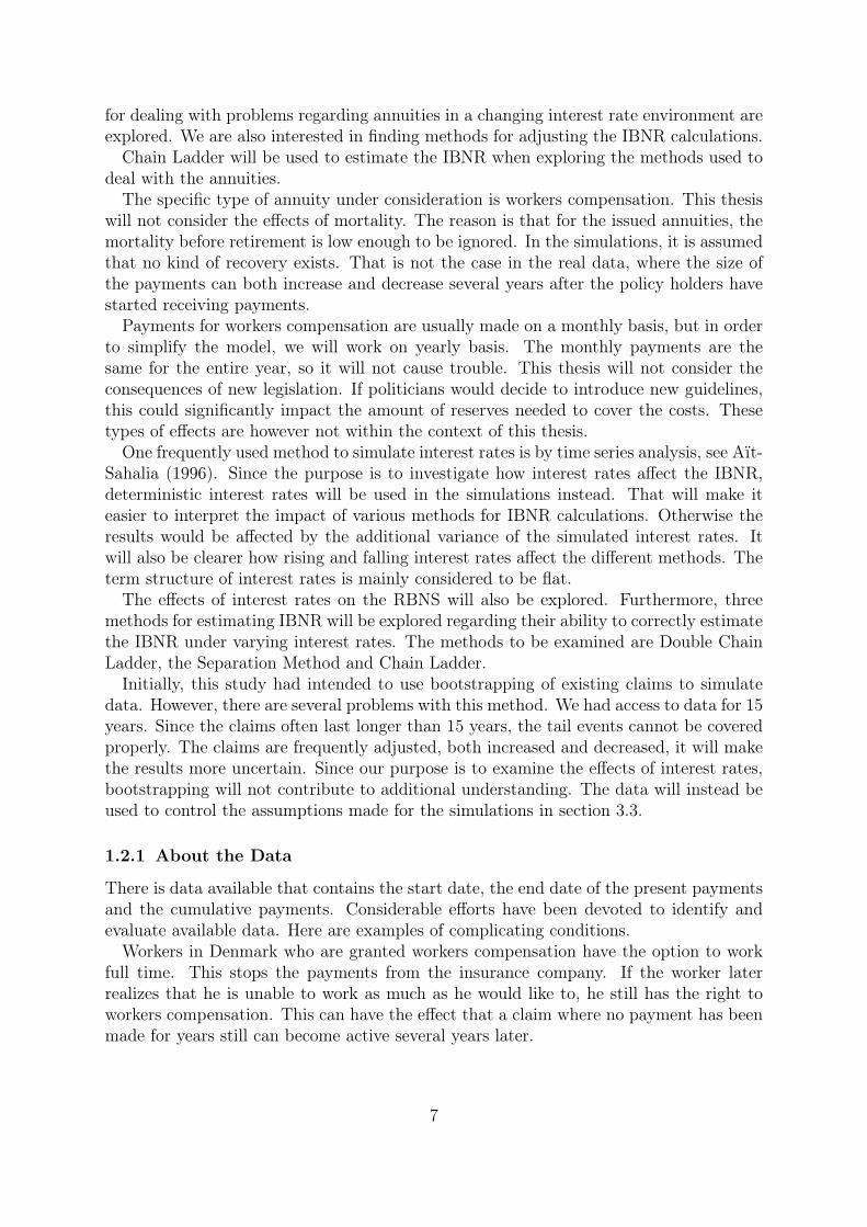
for dealing with problems regarding annuities in a changing interest rate environment areexplored. We are also interested in finding methods for adjusting the IBNR calculations.Chain Ladder will be used to estimate the IBNR when exploring the methods used to
deal with the annuities.The specific type of annuity under consideration is workers compensation. This thesis
will not consider the effects of mortality. The reason is that for the issued annuities, themortality before retirement is low enough to be ignored. In the simulations, it is assumedthat no kind of recovery exists. That is not the case in the real data, where the size ofthe payments can both increase and decrease several years after the policy holders havestarted receiving payments.Payments for workers compensation are usually made on a monthly basis, but in order
to simplify the model, we will work on yearly basis. The monthly payments are thesame for the entire year, so it will not cause trouble. This thesis will not consider theconsequences of new legislation. If politicians would decide to introduce new guidelines,this could significantly impact the amount of reserves needed to cover the costs. Thesetypes of effects are however not within the context of this thesis.One frequently used method to simulate interest rates is by time series analysis, see Aït-
Sahalia (1996). Since the purpose is to investigate how interest rates affect the IBNR,deterministic interest rates will be used in the simulations instead. That will make iteasier to interpret the impact of various methods for IBNR calculations. Otherwise theresults would be affected by the additional variance of the simulated interest rates. Itwill also be clearer how rising and falling interest rates affect the different methods. Theterm structure of interest rates is mainly considered to be flat.The effects of interest rates on the RBNS will also be explored. Furthermore, three
methods for estimating IBNR will be explored regarding their ability to correctly estimatethe IBNR under varying interest rates. The methods to be examined are Double ChainLadder, the Separation Method and Chain Ladder.Initially, this study had intended to use bootstrapping of existing claims to simulate
data. However, there are several problems with this method. We had access to data for 15years. Since the claims often last longer than 15 years, the tail events cannot be coveredproperly. The claims are frequently adjusted, both increased and decreased, it will makethe results more uncertain. Since our purpose is to examine the effects of interest rates,bootstrapping will not contribute to additional understanding. The data will instead beused to control the assumptions made for the simulations in section 3.3.
1.2.1 About the Data
There is data available that contains the start date, the end date of the present paymentsand the cumulative payments. Considerable efforts have been devoted to identify andevaluate available data. Here are examples of complicating conditions.Workers in Denmark who are granted workers compensation have the option to work
full time. This stops the payments from the insurance company. If the worker laterrealizes that he is unable to work as much as he would like to, he still has the right toworkers compensation. This can have the effect that a claim where no payment has beenmade for years still can become active several years later.
7

The cumulative payments were used to calculate the size of the payment for eachannuity by subtracting the total amount paid for one year to the next. This number wasin some cases negative.There is a specific case when negative payments can occur. One of the insurance
company’s costumers has a contract where the insurance company pays a small portionof the cost of the claims. However, the insurance company has to make 100% of thefirst payments to the recipient. Every three months the difference is regulated. Thus, ifan accident occurs and a payment is made in Q4, the majority of that payment wouldthen be refunded by the costumer in Q1. This causes negative payments. When negativepayments occurred, those annuities were removed from the data set. In 2014, the totalpayments were negative in about 2% of the cases.The calculation of the size of the payments is further complicated by the fact that in
Denmark it is possible to get the total annuity payment as a lump sum, rather than asa monthly payment. This will cause the estimation of the annuities to be distorted, asthere are some very large payments made. The largest payment made in 2014 was over 30times larger than the mean. The mean was almost twice the size of the median payment.Another complication is that the claims are numbered by the accidents. Unfortunately
it is not split up into components for each accident. This means that the annuity paymentsare combined with other payments into one sum. Therefore it is not possible to knowfor sure if the payments are just annuities or if there are other payments as well. It isfrequently the case that there is one large payment at the start of the annuity.As an example, table 1 shows the payments for one specific claim. During the first
year, 2002, it is quite obvious that a lump sum was paid. It also looks like an adjustmentin the claims was made in 2004, due to the lower amount paid in 2004 than 2003. Twoadditional lump sums also seem to have been paid in 2006 and 2010.
PaymentsYear 2002 2003 2004 2005 2006 2007 2008 2009 2010 2011
Payment 100 1.75 1.64 1.67 4.81 1.76 1.82 1.88 5.54 1.99
Table 1: Example of how annuity payments can change over time on a yearly basis. Thenumbers represent the total size of the payments in percent relative to the firstyear. The first year both a lump sum and an annuity was present.
One of the main data points for this study is how long time it takes after an accidentoccurs until it is introduced as an annuity. Due to lack of high quality data, the earliestyear it was possible to observe when the claim was introduced as an annuity and the sizeof the claim was 2003. This means that the study has been limited to annuities thatoccurred after 2002.There are still active annuities that occurred earlier than 2002, but unfortunately they
could not be used. Identifying the date when the annuity started to be considered anannuity has been a major complication.After 2005 an annuity flag was introduced to indicate if payments are annuities or not.
Still, that does not mean that the payments were separated into annuities and lump sums,just that the payment includes annuities and might include a lump sum.
8

1.2.2 Separating Annuity Payments from Lump Sums
The annuity part of the payments are the main concern of this thesis. Both annuitypayments and lump sums were present in the same data. Since lump sums are lesssensitive to changes in interest rates than annuities, it was necessary to separate them.Some assumptions, as reviewed below, had to be introduced. They were examined andseemed reasonable given the data.When examining the data on monthly basis, it became apparent that the payments were
not made every month. Sometimes the payments were delayed one, two or even threemonths. In the months following periods when no payment was made, the paymentswere often, but not always, increased to compensate for the lost payments. These typesof larger claims were still considered part of the annuity payment. After a claim wasdetermined, it was possible that the payments were reopened to reflect a readjustmentin the claims. These readjustments were usually in the form of lump sums. Note: Aftergetting in contact with the people responsible for the payments, it seems like the paymentsare made on time, but the data does not reflect this.Assumptions:
1) A single annuity payment was never larger than a few hundred thousand Danishcrowns per year. This was the largest payment recurring on a yearly basis.
2) Payments 400% larger than the median on a monthly basis are the result of a lumpsum in addition to the annuities.
3) When both an annuity and a lump sum is paid to a policy holder, the size of theannuity part of the payment can be estimated by the median of all payments to thatpolicy holder.
4) Annuities have at least four recurring identical payments. This is because the paymentis supposed to be the same every month during a year.
5) If the payment is zero five or more months, subsequent payments are considered lumpsums, unless exactly the same payment reappear for at least two consecutive months.The reason for considering payments that occur after five months of zero payments isthat there are many cases where there are long periods with no payment followed by alump sum. However, sometimes payments may restart after a long period without anypayments. To distinguish the cases when there are two subsequent lump sums fromthe cases when the annuities have restarted, two identical payments are required.
Lump sums were replaced by the median payment for the annuity. This may seem inap-propriate since the replacement was then implicitly depending on the when the durationfirst started. However, when considering the impact this had on the yearly payments,the difference were minuscule compared to what would have been the case if it had beenreplaced by the correct annuity.Since the data kept annuities and lump payments in the same file, the annuities were
marked with a specific flag in 2005 to differentiate them from other claims. A newproblem arouse when claims in the data set frequently had an annuity flag in spite of not
9
having recurring payments. Of the unique claims with an annuity flag, more than 33%had only one payment. In this thesis, payments are not considered as annuities if lessthan four identical payments were made. Therefore those claims have been ignored. Ofthe remaining claims, 45% had at least twelve identical payments.In 2015 the present mean duration of the annuities is about 26.2 years from the start
of each annuity. The standard deviation of this is approximately 10.3. At the time ofcollecting this data, the mean remaining duration for all annuities active in 2015 is 14.4and the standard deviation is 10.2.
1.2.3 Estimating Inflation of the Annuities over Time
The size of the annuity payments increases every year as a consequence of inflation.The inflation of the annuities can be estimated by selecting the annuities that have
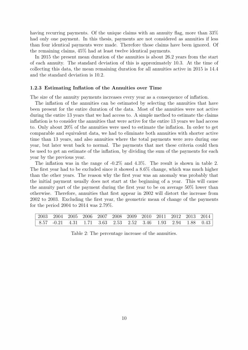
been present for the entire duration of the data. Most of the annuities were not activeduring the entire 13 years that we had access to. A simple method to estimate the claimsinflation is to consider the annuities that were active for the entire 13 years we had accessto. Only about 20% of the annuities were used to estimate the inflation. In order to getcomparable and equivalent data, we had to eliminate both annuities with shorter activetime than 13 years, and also annuities where the total payments were zero during oneyear, but later went back to normal. The payments that met these criteria could thenbe used to get an estimate of the inflation, by dividing the sum of the payments for eachyear by the previous year.The inflation was in the range of -0.2% and 4.3%. The result is shown in table 2.
The first year had to be excluded since it showed a 8.6% change, which was much higherthan the other years. The reason why the first year was an anomaly was probably thatthe initial payment usually does not start at the beginning of a year. This will causethe annuity part of the payment during the first year to be on average 50% lower thanotherwise. Therefore, annuities that first appear in 2002 will distort the increase from2002 to 2003. Excluding the first year, the geometric mean of change of the paymentsfor the period 2004 to 2014 was 2.79%.
2003 2004 2005 2006 2007 2008 2009 2010 2011 2012 2013 20148.57 -0.21 4.31 1.71 3.63 2.53 2.52 3.46 1.93 2.94 1.88 0.43
Table 2: The percentage increase of the annuities.
10
2 Theory
2.1 Terminology
There are two types of outstanding claims to consider in order to get an accurate estimateof the reserves.
RBNS stands for "Reported But Not Settled". This is claims that the insurancecompany is aware of, but the full payment has not yet been carried out. Annuitieswhere the payment has started but the recipient has more payments to collect are RBNS.IBNR stands for "Incurred But Not Reported". It can take years before accidents arereported and the injuries assessed. Often the injuries are not considered so severe thatthe injured person has a right to receive payments from the insurance company. If onlyaccidents known to be severe enough to entitle the policy holder to future paymentswould be counted, the reserve would be much too low to cover all future cost. Thereforeit is necessary to estimate accidents that have happened, but are not yet reported. Itis often a long process to determine the severity of the accident. In the case of workerscompensation, the accidents are often reported, but it can take several years to determineif they will require payments for an extended period. Most recorded accidents in the datawill not become annuities. Despite technically being reported, these claims will be in theIBNR until the severity of the injury is known.
IBNyR (Incurred But Not yet Reported) stands for reserves that have occurred beforethe end of the year, but have not been reported by the end of the year. IBNeR (IncurredBut Not enough Reported) refers to claims that have been reported by the end of theyear, but have not yet been settled. Payments are still expected in the future (Wüthrich2008). IBNeR and RBNS are similar concepts and can be used interchangeably whenworking with "paid" data (Norberg 1986).Claims that are not yet paid will have reserves. The estimate of the amount a claim
will be settled for is called a case reserve. Case reserves are reduced by an appropriateamount when a payment is made. By their nature, case reserves are part of the RBNS,see Atkinson 1989 and irmi.com.
Undetected annuity is used to denote claims that will become annuities, but have notyet been recorded as such. An undetected annuity can be recorded as an accident, butbefore it is settled that it is in fact an annuity, it will be called an undetected annuity.Annuities in the IBNR will be called undetected. Likewise, annuities that are confirmedto be severe enough for the policy holder to require future payments will be called detectedannuities.How long an annuity lasts will be called its duration. This should not be confused with
“duration” in interest theory, where duration is used as measure of the sensitivity of afixed income asset to changes in the interest rate. In this thesis, an annuity that lasts fiveyears is said to have duration of five years, regardless of how the interest rate changes.The size of an annuity refers to the amount paid each year.Workers Compensation is a type of annuity that compensates a worker for loss of
income due to an injury. When a worker gets injured, he will often be unable to work atfull capacity. This will cause a loss of income. This is the type of compensation that willbe considered in this thesis. Workers compensation will only last until the person retires.
11
2.2 Interest Rate Curve
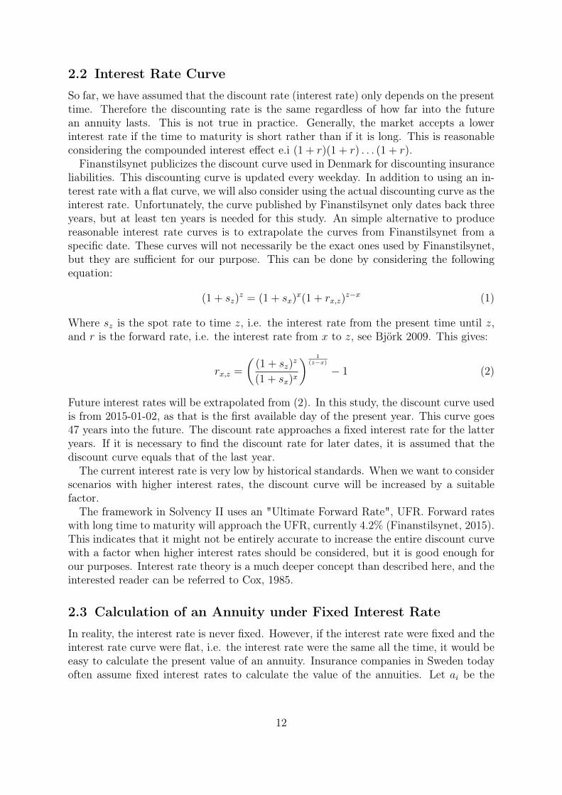
So far, we have assumed that the discount rate (interest rate) only depends on the presenttime. Therefore the discounting rate is the same regardless of how far into the futurean annuity lasts. This is not true in practice. Generally, the market accepts a lowerinterest rate if the time to maturity is short rather than if it is long. This is reasonableconsidering the compounded interest effect e.i (1 + r)(1 + r) . . . (1 + r).Finanstilsynet publicizes the discount curve used in Denmark for discounting insurance
liabilities. This discounting curve is updated every weekday. In addition to using an in-terest rate with a flat curve, we will also consider using the actual discounting curve as theinterest rate. Unfortunately, the curve published by Finanstilsynet only dates back threeyears, but at least ten years is needed for this study. An simple alternative to producereasonable interest rate curves is to extrapolate the curves from Finanstilsynet from aspecific date. These curves will not necessarily be the exact ones used by Finanstilsynet,but they are sufficient for our purpose. This can be done by considering the followingequation:
(1 + sz)z = (1 + sx)x(1 + rx,z)
z−x (1)
Where sz is the spot rate to time z, i.e. the interest rate from the present time until z,and r is the forward rate, i.e. the interest rate from x to z, see Björk 2009. This gives:
rx,z =
((1 + sz)
z
(1 + sx)x
) 1(z−x)
− 1 (2)
Future interest rates will be extrapolated from (2). In this study, the discount curve usedis from 2015-01-02, as that is the first available day of the present year. This curve goes47 years into the future. The discount rate approaches a fixed interest rate for the latteryears. If it is necessary to find the discount rate for later dates, it is assumed that thediscount curve equals that of the last year.The current interest rate is very low by historical standards. When we want to consider
scenarios with higher interest rates, the discount curve will be increased by a suitablefactor.The framework in Solvency II uses an "Ultimate Forward Rate", UFR. Forward rates
with long time to maturity will approach the UFR, currently 4.2% (Finanstilsynet, 2015).This indicates that it might not be entirely accurate to increase the entire discount curvewith a factor when higher interest rates should be considered, but it is good enough forour purposes. Interest rate theory is a much deeper concept than described here, and theinterested reader can be referred to Cox, 1985.
2.3 Calculation of an Annuity under Fixed Interest Rate
In reality, the interest rate is never fixed. However, if the interest rate were fixed and theinterest rate curve were flat, i.e. the interest rate were the same all the time, it would beeasy to calculate the present value of an annuity. Insurance companies in Sweden todayoften assume fixed interest rates to calculate the value of the annuities. Let ai be the
12

payment, n the time for the final payment and si the spot interest rate. Since we wantto calculate the discounted payments, the present value (PV) is then calculated as in (3).
PV =n∑i
ai(1 + si)i
(3)
If all ai and si were identical, it can be calculated by the geometric sum, since
PV = a(1 + s)−1 + a(1 + s)−2 + . . .+ a(1 + s)−n
PV (1 + s) = a+ a(1 + s)−1 + . . .+ a(1 + s)1−n
PV (1 + s)− PV = a− a(1 + s)−n
PV ((1 + s)− 1) = a(1− (1 + s)−n)
PV = a1− (1 + s)−n
s(4)
In practice the payment a is often increased over time to compensate for inflation. Thiscan be compensated for by simply adjusting the interest rate, s, used to discount theannuity. This simplified method to calculate the present value of an annuity will notbe allowed under Solvency II regulations, where an interest rate curve has to be usedinstead.
2.4 Estimating the IBNR
When accidents occur the policy holder will have a claim on the insurance company. Howlarge the total claim amount will be is not known at the time of the accident. This isespecially true for personal injury when the claim will be paid as an annuity over manyyears. Since the insurance company needs to know how large the total claim amountwill be in order to properly set aside reserves to cover the future costs, there are manymethods for estimating the claim. Three methods will be explored in this thesis: ChainLadder, Double Chain Ladder and the Separation Method.
2.4.1 Chain Ladder Method (CLM)
Due to its simplicity, the Chain Ladder Method, (CLM), is arguably the most popularmethod for estimating outstanding claims, both in theory and in practice, (Wüthrich,2008). The idea of the method is that present claims will approximately develop like pastclaims. This will be used to estimate the total reserve. "Exogeneous influences", suchas inflation, can cause the claims to develop in a manner they did not do before, andtherefore give misguided results (Taylor, 1977).It can be assumed that the data is available on triangle form. Let the set Ω = (i, j) :
i = 1, . . . ,m, j = 1, . . . ,m; i + j ≤ m − 1 be the observable data available at a time m
13
from the first point in the triangle. Note that Ω can be interpreted as the upper part ofa triangle. The lower part of the triangle, m ≤ i+ j ≤ 2m is unknown at time m.Let the cumulative paid amount be Ci,j, where i is the accident year and j is the
development year, i.e. how many years it has been since the accident occurred. Let∆m = Ci,j ∈ Ω. The total payments in year i, paid j periods from i is then denotedCi,j.The idea is that the cumulative claims will increase as much as they have done in the
past for a specific development year. Cumulative claims are assumed to be independentfor different accident years i. Let the last development period, also known as ultimo, be Jand furthermore let the last accident year be I. It is assumed that the claims for a specificdevelopment year is expected to increase by a fixed amount for a specific period. Then wecan introduce development factors f1, ..., fJ−1 > 0, such that E[Ci,j|Ci,j−1] = fj−1Ci,j−1.Estimates for fj can be found by:
fj =
∑I−kk=1 Ck,j+1∑I−kk=1 Ck,j
j = 1, . . . , I − 1
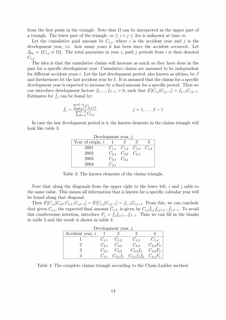
In case the last development period is 4, the known elements in the claims triangle willlook like table 3.
Development year, jYear of origin, i 1 2 3 4
2001 C1,1 C1,2 C1,3 C1,4
2002 C2,1 C2,2 C2,3
2003 C3,1 C3,2
2004 C4,1
Table 3: The known elements of the claims triangle.
Note that along the diagonals from the upper right to the lower left, i and j adds tothe same value. This means all information that is known for a specific calendar year willbe found along that diagonal.Then E[Ci,j|Ci,0, Ci,1, Ci,j−1] = E[Ci,j|Ci,j−1] = fj−1Ci,j−1. From this, we can conclude
that given Ci,j, the expected final amount Ci,J , is given by Ci,j fi,j fi,j+1...fi,J−1. To avoidthis cumbersome notation, introduce Fj = fjfj+1...fJ−1. Thus we can fill in the blanksin table 3 and the result is shown in table 4.
Development year, jAccident year, i 1 2 3 4
1 C1,1 C1,2 C1,3 C1,4
2 C2,1 C2,2 C2,3 C2,3F3
3 C3,1 C3,2 C3,2f2 C3,2F2
4 C4,1 C4,1f1 C4,1f1f2 C4,1F1
Table 4: The complete claims triangle according to the Chain Ladder method.
14
The IBNR is the sum of the last column, C1,J . . . CI,J , minus the last known diagonal,C1,J . . . CI,1.Chain Ladder can be performed on payments or the case reserves, see (Mack 1993).
In method A), described in section 2.6.1, it is used on payments combined with casereserves. This could be an issue, as the development factors are lower when using casereserves than payments. However, we will assume that no assumptions are broken byconsidering case reserves combined with payments.
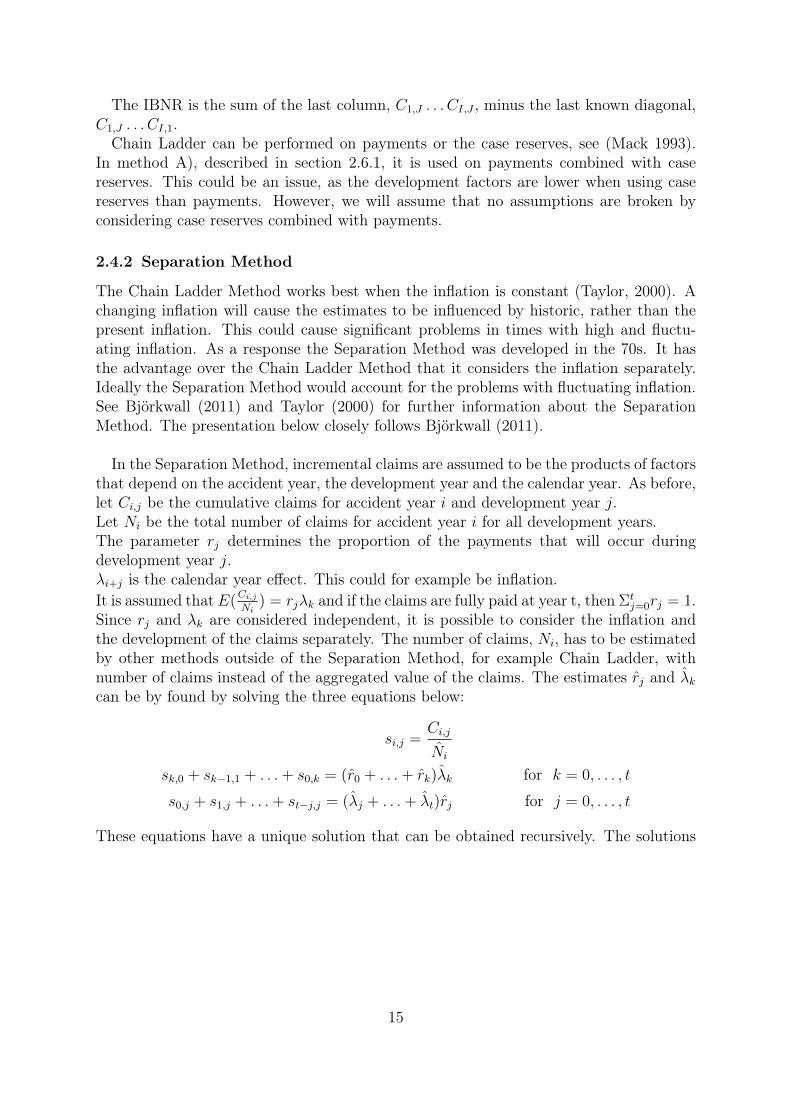
2.4.2 Separation Method
The Chain Ladder Method works best when the inflation is constant (Taylor, 2000). Achanging inflation will cause the estimates to be influenced by historic, rather than thepresent inflation. This could cause significant problems in times with high and fluctu-ating inflation. As a response the Separation Method was developed in the 70s. It hasthe advantage over the Chain Ladder Method that it considers the inflation separately.Ideally the Separation Method would account for the problems with fluctuating inflation.See Björkwall (2011) and Taylor (2000) for further information about the SeparationMethod. The presentation below closely follows Björkwall (2011).
In the Separation Method, incremental claims are assumed to be the products of factorsthat depend on the accident year, the development year and the calendar year. As before,let Ci,j be the cumulative claims for accident year i and development year j.Let Ni be the total number of claims for accident year i for all development years.The parameter rj determines the proportion of the payments that will occur duringdevelopment year j.λi+j is the calendar year effect. This could for example be inflation.It is assumed that E(
Ci,j
Ni) = rjλk and if the claims are fully paid at year t, then Σt
j=0rj = 1.Since rj and λk are considered independent, it is possible to consider the inflation andthe development of the claims separately. The number of claims, Ni, has to be estimatedby other methods outside of the Separation Method, for example Chain Ladder, withnumber of claims instead of the aggregated value of the claims. The estimates rj and λkcan be by found by solving the three equations below:
si,j =Ci,j
Ni
sk,0 + sk−1,1 + . . .+ s0,k = (r0 + . . .+ rk)λk for k = 0, . . . , t
s0,j + s1,j + . . .+ st−j,j = (λj + . . .+ λt)rj for j = 0, . . . , t
These equations have a unique solution that can be obtained recursively. The solutions
15
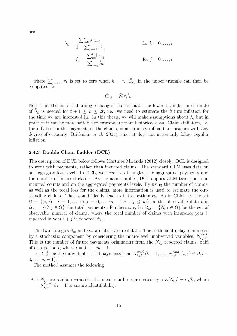
are
λk =
∑ki=0 si,k−i
1−∑t
j=k+1 r jfor k = 0, . . . , t
rk =
∑t−ji=0 si,j∑tk=j λk
for j = 0, . . . , t
where∑t
j=k+1 rk is set to zero when k = t. Ci,j in the upper triangle can then becomputed by
Ci,j = Nirjλk
Note that the historical triangle changes. To estimate the lower triangle, an estimateof λk is needed for t + 1 ≤ k ≤ 2t, i.e. we need to estimate the future inflation forthe time we are interested in. In this thesis, we will make assumptions about λ, but inpractice it can be more suitable to extrapolate from historical data. Claims inflation, i.e.the inflation in the payments of the claims, is notoriously difficult to measure with anydegree of certainty (Brickman et al. 2005), since it does not necessarily follow regularinflation.
2.4.3 Double Chain Ladder (DCL)
The description of DCL below follows Martinez Miranda (2012) closely. DCL is designedto work with payments, rather than incurred claims. The standard CLM uses data onan aggregate loss level. In DCL, we need two triangles, the aggregated payments andthe number of incurred claims. As the name implies, DCL applies CLM twice, both onincurred counts and on the aggregated payments levels. By using the number of claims,as well as the total loss for the claims, more information is used to estimate the out-standing claims. That would ideally lead to better estimates. As in CLM, let the setΩ = (i, j) : i = 1, . . . ,m, j = 0, . . . ,m − 1; i + j ≤ m be the observable data and∆m = Ci,j ∈ Ω the total payments. Furthermore, let ℵm = Ni,j ∈ Ω be the set ofobservable number of claims, where the total number of claims with insurance year i,reported in year i+ j is denoted Ni,j.
The two triangles ℵm and ∆m are observed real data. The settlement delay is modeledby a stochastic component by considering the micro-level unobserved variables, Npaid
i,j,l .This is the number of future payments originating from the Ni,j reported claims, paidafter a period l, where l = 0, . . . ,m− 1.Let Y (k)
i,j,l be the individual settled payments from Npaidi,j,l (k = 1, . . . , Npaid
i,j,l , (i, j) ∈ Ω, l =0, . . . ,m− 1).The method assumes the following:
A1) Nij are random variables. Its mean can be represented by a E[Ni,j] = αiβj, where∑m−1j=0 βj = 1 to ensure identifiability.
16
A2) E[Npaidi,j,l |ℵ] = Ni,jπl is the mean of the RBNS delay variables, for (i, j) ∈ Ω, l =
0, . . . ,m− 1
A3) When conditioning on the number of payments, the mean of the individual pay-ments size is given by E[Y
(k)i,j,l|N
paidi,j,l ] = µlγi
In the special case with exactly one payment per claim, A2) can be replaced by A2’)and we can add A4):
A2’) The number of paid claims follow a multinomial distribution, given Ni,j. Thus(Npaid
i,j,0 , . . . , Npaidi,j,d ) ∼ Multi(Ni,j; p0, . . . , pd), where d is the maximum delay. Let
p = (p0, . . . , pd) denote the delay probabilities. Thus∑d
l=0 pl = 1 and 0 < pl < 1,∀l
A4) Assume that Y (k)i,j,l are independent of the counts Ni,j
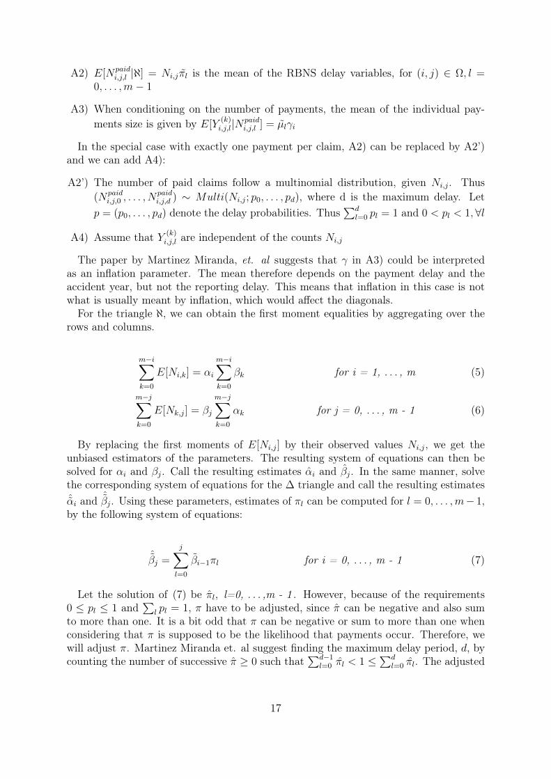
The paper by Martinez Miranda, et. al suggests that γ in A3) could be interpretedas an inflation parameter. The mean therefore depends on the payment delay and theaccident year, but not the reporting delay. This means that inflation in this case is notwhat is usually meant by inflation, which would affect the diagonals.For the triangle ℵ, we can obtain the first moment equalities by aggregating over the
rows and columns.
m−i∑k=0
E[Ni,k] = αi
m−i∑k=0
βk for i = 1, . . . , m (5)
m−j∑k=0
E[Nk,j] = βj
m−j∑k=0
αk for j = 0, . . . , m - 1 (6)
By replacing the first moments of E[Ni,j] by their observed values Ni,j, we get theunbiased estimators of the parameters. The resulting system of equations can then besolved for αi and βj. Call the resulting estimates αi and βj. In the same manner, solvethe corresponding system of equations for the ∆ triangle and call the resulting estimatesˆαi and
ˆβj. Using these parameters, estimates of πl can be computed for l = 0, . . . ,m− 1,by the following system of equations:
ˆβj =
j∑l=0
βi−1πl for i = 0, . . . , m - 1 (7)
Let the solution of (7) be πl, l=0, . . . ,m - 1 . However, because of the requirements0 ≤ pl ≤ 1 and
∑l pl = 1, π have to be adjusted, since π can be negative and also sum
to more than one. It is a bit odd that π can be negative or sum to more than one whenconsidering that π is supposed to be the likelihood that payments occur. Therefore, wewill adjust π. Martinez Miranda et. al suggest finding the maximum delay period, d, bycounting the number of successive π ≥ 0 such that
∑d−1l=0 πl < 1 ≤
∑dl=0 πl. The adjusted
17
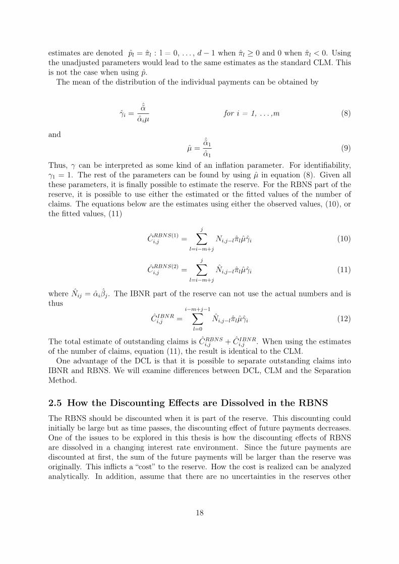
estimates are denoted pl = πl : l = 0, . . . , d− 1 when πl ≥ 0 and 0 when πl < 0. Usingthe unadjusted parameters would lead to the same estimates as the standard CLM. Thisis not the case when using p.The mean of the distribution of the individual payments can be obtained by
γi =ˆα
αiµfor i = 1, . . . ,m (8)
and
µ =ˆα1
α1
(9)
Thus, γ can be interpreted as some kind of an inflation parameter. For identifiability,γ1 = 1. The rest of the parameters can be found by using µ in equation (8). Given allthese parameters, it is finally possible to estimate the reserve. For the RBNS part of thereserve, it is possible to use either the estimated or the fitted values of the number ofclaims. The equations below are the estimates using either the observed values, (10), orthe fitted values, (11)
CRBNS(1)i,j =
j∑l=i−m+j
Ni,j−lπlµγi (10)
CRBNS(2)i,j =
j∑l=i−m+j
Ni,j−lπlµγi (11)
where Nij = αiβj. The IBNR part of the reserve can not use the actual numbers and isthus
CIBNRi,j =
i−m+j−1∑l=0
Ni,j−lπlµγi (12)
The total estimate of outstanding claims is CRBNSi,j + CIBNR
i,j . When using the estimatesof the number of claims, equation (11), the result is identical to the CLM.One advantage of the DCL is that it is possible to separate outstanding claims into
IBNR and RBNS. We will examine differences between DCL, CLM and the SeparationMethod.
2.5 How the Discounting Effects are Dissolved in the RBNS
The RBNS should be discounted when it is part of the reserve. This discounting couldinitially be large but as time passes, the discounting effect of future payments decreases.One of the issues to be explored in this thesis is how the discounting effects of RBNSare dissolved in a changing interest rate environment. Since the future payments arediscounted at first, the sum of the future payments will be larger than the reserve wasoriginally. This inflicts a “cost” to the reserve. How the cost is realized can be analyzedanalytically. In addition, assume that there are no uncertainties in the reserves other
18
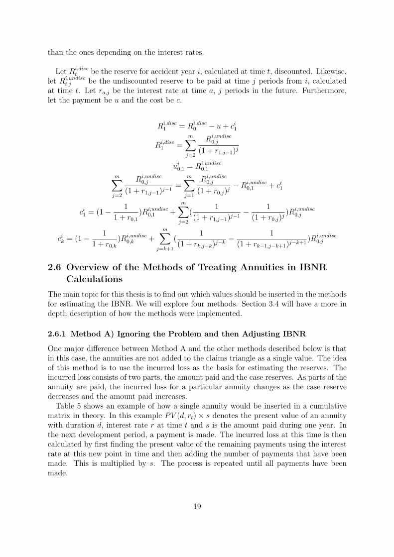
than the ones depending on the interest rates.
Let Ri,disct be the reserve for accident year i, calculated at time t, discounted. Likewise,
let Ri,undisct,j be the undiscounted reserve to be paid at time j periods from i, calculated
at time t. Let ra,j be the interest rate at time a, j periods in the future. Furthermore,let the payment be u and the cost be c.
Ri,disc1 = Ri,disc
0 − u+ ci1
Ri,disc1 =
m∑j=2
Ri,undisc0,j
(1 + r1,j−1)j
ui0,1 = Ri,undisc0,1
m∑j=2
Ri,undisc0,j
(1 + r1,j−1)j−1=
m∑j=1
Ri,undisc0,j
(1 + r0,j)j−Ri,undisc
0,1 + ci1
ci1 = (1− 1
1 + r0,1)Ri,undisc
0,1 +m∑j=2
(1
(1 + r1,j−1)j−1− 1
(1 + r0,j)j)Ri,undisc
0,j
cik = (1− 1
1 + r0,k)Ri,undisc
0,k +m∑
j=k+1
(1
(1 + rk,j−k)j−k− 1
(1 + rk−1,j−k+1)j−k+1)Ri,undisc
0,j
2.6 Overview of the Methods of Treating Annuities in IBNRCalculations
The main topic for this thesis is to find out which values should be inserted in the methodsfor estimating the IBNR. We will explore four methods. Section 3.4 will have a more indepth description of how the methods were implemented.
2.6.1 Method A) Ignoring the Problem and then Adjusting IBNR
One major difference between Method A and the other methods described below is thatin this case, the annuities are not added to the claims triangle as a single value. The ideaof this method is to use the incurred loss as the basis for estimating the reserves. Theincurred loss consists of two parts, the amount paid and the case reserves. As parts of theannuity are paid, the incurred loss for a particular annuity changes as the case reservedecreases and the amount paid increases.Table 5 shows an example of how a single annuity would be inserted in a cumulative
matrix in theory. In this example PV (d, rt)× s denotes the present value of an annuitywith duration d, interest rate r at time t and s is the amount paid during one year. Inthe next development period, a payment is made. The incurred loss at this time is thencalculated by first finding the present value of the remaining payments using the interestrate at this new point in time and then adding the number of payments that have beenmade. This is multiplied by s. The process is repeated until all payments have beenmade.
19

Development year, jYear of origin, i 1 2 3
PV (d, r1)× s (PV (d− 1, r2) + 1)× s (PV (d− 2, r3) + 2)× s
Table 5: Example of how an annuity would be inserted in a cumulative triangle in methodA in theory. The annuity is detected in the first development year. The presentyear is year 3. Note how different interest rates and durations are used and thatpayments are made.
Chain-Ladder or some other method for estimating the reserves could then be usedto find the total reserve. However, that will project the total undiscounted payments.Since the reserve should be discounted, this method will overestimate the total reserve.Therefore, we need to remove the discounting effect of the RBNS. The discounting effectis found by examining the total payments that will be done on all the known claims andsubtracting the sum of the last diagonal in the cumulative triangle.The advantage of this method is that it is easy to find the appropriate values to insert
in the triangles if each claim is associated with an incurred loss amount for each year.
2.6.2 Method B) Pretend the Annuity is Bought
This is the standard method used in most insurance companies in Sweden today. Workwith claims triangles on an incremental basis. When the annuity is determined, thepresent value of the annuity is calculated by the geometric sum and entered into thetriangle. Table 6 shows an example of how an annuity would be inserted in a cumulativetriangle in method B. The notation is the same as in the previous method. When theannuity is detected, the present value is calculated and inserted in the triangle. Thisvalue never changes, regardless of the interest rate or the payments made. Note that thisexample only shows a single annuity.
Development year, jYear of origin, i 1 2 3 4
PV (d, r1)× s PV (d, r1)× s PV (d, r1)× s PV (d, r1)× s
Table 6: Example of how a single annuity would be inserted in a cumulative triangle inmethod B. The annuity is detected in the first development year. The presentyear is year 4. Note that the interest rate used is the one present at the yearthe annuity was detected and that there are no payments made. If a claim wasdetected in year 4, that claim would be discounted with r4.
The IBNR is then calculated on basis of these valuations with some method for IBNRcalculations. If the discount rate were the same all the time, this would work well.The problem is that the interest rate changes over time. Changing interest rates willcause a different interest rate to be used in the geometric sum for different years. Thiswill cause the triangles to be affected by the interest rate active at the time of theinception of previous interest rates. In case the interest rate previously was higher thanthe current interest rate, this would cause the value inserted in the triangle to be lower
20
than appropriate and vice versa. Likewise, if the payments are adjusted for inflation, thatwould also affect the payments. It is possible to combine inflation and interest rate in thegeometric series to get a better estimate for the final payments. Because the historicaldata is used to get an estimate of the payments to come, the best estimate of the presentreserve would be if the interest and inflation rate would have been the same in the pastas it is today. Since this is not the case, the data can be adjusted in order to get abetter estimate of the current reserves. One method for adjusting this will be exploredsection 2.6.3. An advantage of using method B is that there is no need to keep trackof previous claims. When updating a triangle, only the latest diagonal will be changed.This diagonal only depends on the current interest rate and indexing.
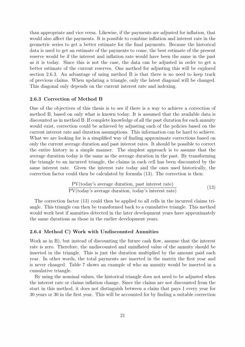
2.6.3 Correction of Method B
One of the objectives of this thesis is to see if there is a way to achieve a correction ofmethod B, based on only what is known today. It is assumed that the available data isdiscounted as in method B. If complete knowledge of all the past duration for each annuitywould exist, correction could be achieved by adjusting each of the policies based on thecurrent interest rate and duration assumptions. This information can be hard to achieve.What we are looking for is a simplified way of finding approximate corrections based ononly the current average duration and past interest rates. It should be possible to correctthe entire history in a simple manner. The simplest approach is to assume that theaverage duration today is the same as the average duration in the past. By transformingthe triangle to an incurred triangle, the claims in each cell has been discounted by thesame interest rate. Given the interest rate today and the ones used historically, thecorrection factor could then be calculated by formula (13). The correction is then:
PV(today’s average duration, past interest rate)PV(today’s average duration, today’s interest rate)
(13)
The correction factor (13) could then be applied to all cells in the incurred claims tri-angle. This triangle can then be transformed back to a cumulative triangle. This methodwould work best if annuities detected in the later development years have approximatelythe same durations as those in the earlier development years.
2.6.4 Method C) Work with Undiscounted Annuities
Work as in B), but instead of discounting the future cash flow, assume that the interestrate is zero. Therefore, the undiscounted and uninflated value of the annuity should beinserted in the triangle. This is just the duration multiplied by the amount paid eachyear. In other words, the total payments are inserted in the matrix the first year andis never changed. Table 7 shows an example of who an annuity would be inserted in acumulative triangle.By using the nominal values, the historical triangle does not need to be adjusted when
the interest rate or claims inflation change. Since the claims are not discounted from thestart in this method, it does not distinguish between a claim that pays 1 every year for30 years or 30 in the first year. This will be accounted for by finding a suitable correction
21

Development year, jYear of origin, i 1 2 3 4
d× s d× s d× s d× s
Table 7: Example of how an annuity would be inserted in a cumulative triangle in methodC. The annuity is detected in the first development year. The present year isyear 4. Note that interest rates are not present.
factor, similar to that in 2.6.3. In this case, the correction will be done by equation (14),which calculates the proportion of the present value of all claims relative to the nominalamount. This is a reasonable approximation when everything is relatively homogeneous.
∑i PV (di, today’s interest rate)× si∑
i di × si(14)
The correction factor, (14), will be multiplied by the IBNR after all the IBNR iscalculated in the usual manner. This leads to an estimate that is comparable to that ofthe other methods.The advantage of method C is that the reserving is independent of the interest rate.
It will therefore be easier to adjust the triangle according to the present interest rate inorder to get an accurate reserve.
2.6.5 Method D) Present Interest Rate
In order to get the ideal value of the reserve, we would have to adjust everything to thepresent assumptions. For that purpose we need to keep all the values of the original claimsundiscounted and unindexed. When the reserve is calculated, the present interest rateand indexing will be used to discount the annuities. Then keep working as in B. Table 8shows an example of how an annuity would be inserted in a triangle in this method. Itshould be noted that the interest rate used is the latest interest rate. That interest rateis not known at the time the annuity was first detected. Therefore the claims trianglehas to be updated every year.
Development year, jYear of origin, i 1 2 3 4
PV (d, r4)× s PV (d, r4)× s PV (d, r4)× s PV (d, r4)× s
Table 8: Example of how an annuity would be inserted in a cumulative triangle in methodD. The annuity is detected in the first development year. The present year isyear 4. Note that the interest rate used is the present interest rate.
The differences between method D and B, is that B does not update the values insertedin the triangle. The interest rate and indexing that was present at the time the annuitywas recorded will always be used for that annuity, regardless of the current state. Inorder to use method D, we need to keep the claims and indexing separate from the IBNRcalculations.
22

2.6.6 The True Values of the Annuities
When the data is simulated it is possible to know all future claims. This is obviouslynot possible in the real world. However, having access to the complete data allows usto compute the true value. In an ideal world, this is the value we would want to find inour previous methods. It is only possible to calculate in simulations when all the futureclaims are known. This method will be used as a reference to compare how well the othermethods preform. It is done by discounting all future payments with the present interestrate.
23
3 MethodThis section will describe the details of how the study was implemented. The reader whodoes not have an interest in knowing these details could skip this section and proceed tothe results.
3.1 Structuring the Data
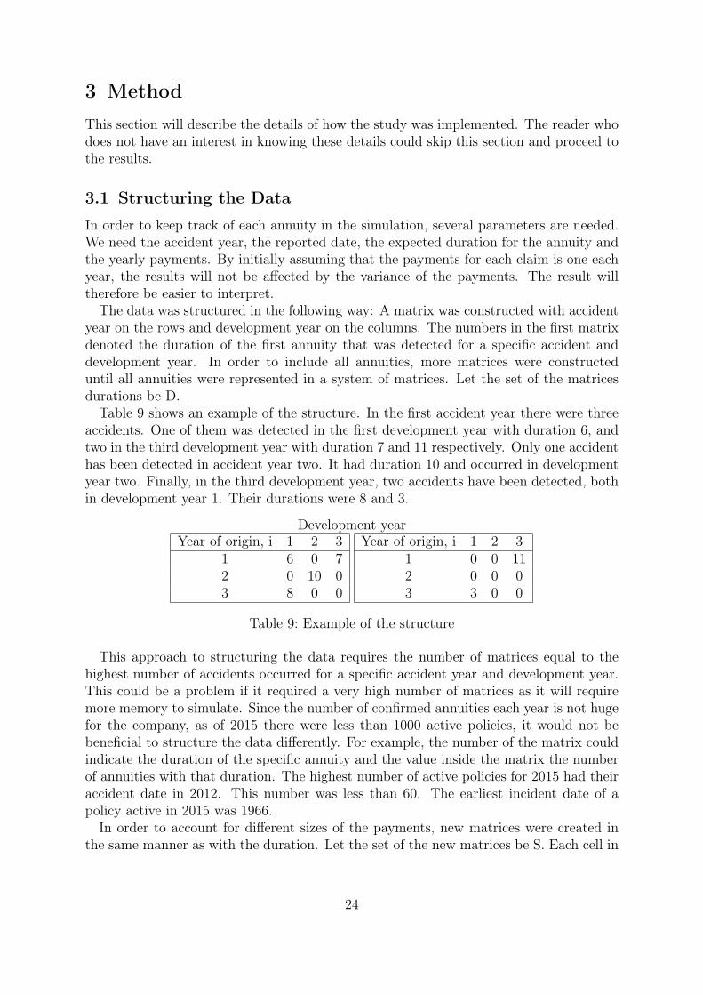
In order to keep track of each annuity in the simulation, several parameters are needed.We need the accident year, the reported date, the expected duration for the annuity andthe yearly payments. By initially assuming that the payments for each claim is one eachyear, the results will not be affected by the variance of the payments. The result willtherefore be easier to interpret.The data was structured in the following way: A matrix was constructed with accident
year on the rows and development year on the columns. The numbers in the first matrixdenoted the duration of the first annuity that was detected for a specific accident anddevelopment year. In order to include all annuities, more matrices were constructeduntil all annuities were represented in a system of matrices. Let the set of the matricesdurations be D.Table 9 shows an example of the structure. In the first accident year there were three
accidents. One of them was detected in the first development year with duration 6, andtwo in the third development year with duration 7 and 11 respectively. Only one accidenthas been detected in accident year two. It had duration 10 and occurred in developmentyear two. Finally, in the third development year, two accidents have been detected, bothin development year 1. Their durations were 8 and 3.
Development yearYear of origin, i 1 2 3
1 6 0 72 0 10 03 8 0 0
Year of origin, i 1 2 31 0 0 112 0 0 03 3 0 0
Table 9: Example of the structure
This approach to structuring the data requires the number of matrices equal to thehighest number of accidents occurred for a specific accident year and development year.This could be a problem if it required a very high number of matrices as it will requiremore memory to simulate. Since the number of confirmed annuities each year is not hugefor the company, as of 2015 there were less than 1000 active policies, it would not bebeneficial to structure the data differently. For example, the number of the matrix couldindicate the duration of the specific annuity and the value inside the matrix the numberof annuities with that duration. The highest number of active policies for 2015 had theiraccident date in 2012. This number was less than 60. The earliest incident date of apolicy active in 2015 was 1966.In order to account for different sizes of the payments, new matrices were created in
the same manner as with the duration. Let the set of the new matrices be S. Each cell in
24
S corresponded to a cell in D. The cells in S represented the size of the claims. The totaloutstanding payments could then be obtained by multiplying the two sets of matrices.When simulating the data, it is possible to get a complete set of matrices where the
last development year is known for every accident year. In reality, this is not possible.Realistically, k years from the accident year, it is only possible to know what happenedat development year k + 1. For the last accident year only the first development yearwould be known.
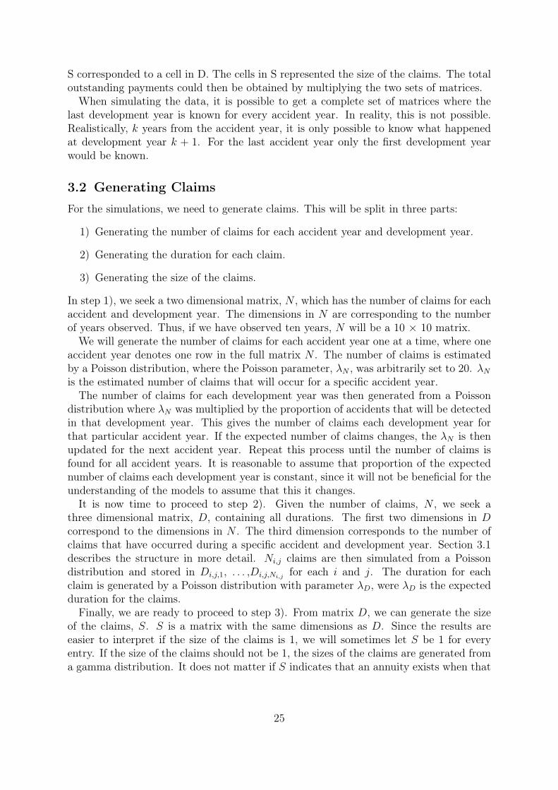
3.2 Generating Claims
For the simulations, we need to generate claims. This will be split in three parts:
1) Generating the number of claims for each accident year and development year.
2) Generating the duration for each claim.
3) Generating the size of the claims.
In step 1), we seek a two dimensional matrix, N , which has the number of claims for eachaccident and development year. The dimensions in N are corresponding to the numberof years observed. Thus, if we have observed ten years, N will be a 10 × 10 matrix.We will generate the number of claims for each accident year one at a time, where one
accident year denotes one row in the full matrix N . The number of claims is estimatedby a Poisson distribution, where the Poisson parameter, λN , was arbitrarily set to 20. λNis the estimated number of claims that will occur for a specific accident year.The number of claims for each development year was then generated from a Poisson
distribution where λN was multiplied by the proportion of accidents that will be detectedin that development year. This gives the number of claims each development year forthat particular accident year. If the expected number of claims changes, the λN is thenupdated for the next accident year. Repeat this process until the number of claims isfound for all accident years. It is reasonable to assume that proportion of the expectednumber of claims each development year is constant, since it will not be beneficial for theunderstanding of the models to assume that this it changes.It is now time to proceed to step 2). Given the number of claims, N , we seek a
three dimensional matrix, D, containing all durations. The first two dimensions in Dcorrespond to the dimensions in N . The third dimension corresponds to the number ofclaims that have occurred during a specific accident and development year. Section 3.1describes the structure in more detail. Ni,j claims are then simulated from a Poissondistribution and stored in Di,j,1, . . . ,Di,j,Ni,j
for each i and j. The duration for eachclaim is generated by a Poisson distribution with parameter λD, were λD is the expectedduration for the claims.Finally, we are ready to proceed to step 3). From matrix D, we can generate the size
of the claims, S. S is a matrix with the same dimensions as D. Since the results areeasier to interpret if the size of the claims is 1, we will sometimes let S be 1 for everyentry. If the size of the claims should not be 1, the sizes of the claims are generated froma gamma distribution. It does not matter if S indicates that an annuity exists when that
25

is not the case, since it can be interpreted as a claim with duration of 0, which will notbe included in any calculations anyway.
3.3 Selection of Parameters and Assumptions
In order to compare the methods, data had to be simulated. The following parameterswere used to generate data.
1) The number of simulations was set to 10 000.
2) The size of the matrix was determined to be 10 × 10. This size was deemed largeenough to find effects due to inflation, but not so large that it affected the computa-tional time.
3) The number of claims that occurred in each cell was simulated from a Poisson distri-bution with parameter λN = 60.
4) The size of each claims was simulated from a gamma distribution with shape parameter10 and rate parameter 1, i.e. it has the expected value 10.
5) Inflation affected all claims equally, i.e. the size of the claims was multiplied by thecumulative inflation.
6) The proportions of claims that occurred during a specific development year was setto 0.06 for the first year, 0.20 for the second, and 0.34, 0.30, 0.06, 0.04 for the thirdto sixth year. This is very close to the actual ratios according to the data.
Assumptions about the correlations: Given this method to generate data, there areseveral implicit assumptions about the correlations. Explicitly:
A1) There is no correlation between the number of claims for an accident year or acalendar year.
A2) There is no correlation between the number of claims and the size of the claims.
A3) There is no correlation between the delay and the size of the claims, when theinflation effect is discounted.
A4) The proportion of claims that occur during a specific development year relative tothe accident year remains constant.
These assumptions were made to isolate the interest rate effect. A1) was introducedto study the interest rate effect in constant conditions. A2) is a reasonable assumptionif all claims are independent of each other. If a large company had a huge accidentwhich affected many workers, that might distort this assumption, but introducing suchdependencies would just add variance to the results, without aiding the interpretation.A3) might seem like a "large" assumption, specifically that there is no correlation between
26
the size of the claim and the development year. Is is easy to imagine that a severe accidentwould be treated differently than a small one. This assumption is however verified in thedata for workers compensation used in this thesis, which gives a confidence interval of(-0.12; 0.03) for the hypothesis that the correlation is 0. A few scenarios that explorewhat would happen if A3) was not met is also included in order to make the results moregeneral and applicable to other kinds of insurance.Note: Assumption A1 is not supported by the data. There is a significant correlation
between the number of claims and the calendar year. The number of claims is increasingwith time. Some scenarios will explore the methods deal with increasing number ofclaims. In those cases, the number of claims will be assumed to change with a constantrate for each year.Note: This way of generating data assumes that there are new accidents detected in
periods 1 - 6 but nothing after that. There were a few claims reported after more than 6years, but they were very infrequent.Note: The inflation of the claims is assumed to affect the claims along the diagonals.
This inflation is the calendar year effect. Should there be a difference in the size of theclaims with different reported delay times, this is not included in this effect. No sucheffect was detected in the data.The upper triangle generated this way was then subjected to the three methods for
estimating the annuity reserve.
3.4 Detailed Description of the Implementation of the Methods
The following chapter is only recommended for the reader with a great interest in thedetails of how the methods were implemented and not necessary to understand the re-sults. The reader mainly interested in the results is recommended to proceed to section 4.
Each of the methods starts by receiving three parameters. Let the duration of theclaims be D and the size of the claims be S. S and D are matrices of the form describedin section 3.1. Furthermore, let R be a vector with the interest rate for the observedtime. R is deterministic. The values of R depend on the investigated scenario.
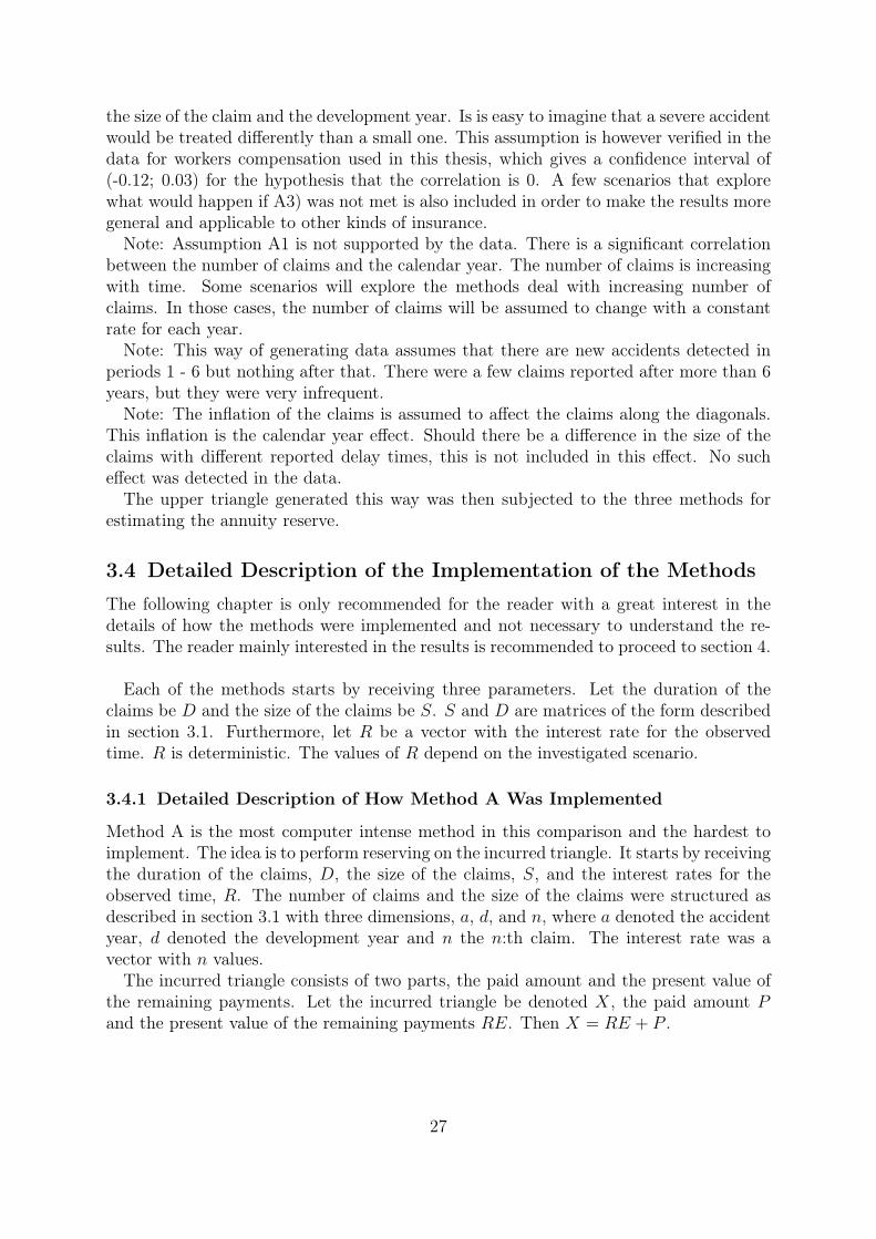
3.4.1 Detailed Description of How Method A Was Implemented
Method A is the most computer intense method in this comparison and the hardest toimplement. The idea is to perform reserving on the incurred triangle. It starts by receivingthe duration of the claims, D, the size of the claims, S, and the interest rates for theobserved time, R. The number of claims and the size of the claims were structured asdescribed in section 3.1 with three dimensions, a, d, and n, where a denoted the accidentyear, d denoted the development year and n the n:th claim. The interest rate was avector with n values.The incurred triangle consists of two parts, the paid amount and the present value of
the remaining payments. Let the incurred triangle be denoted X, the paid amount Pand the present value of the remaining payments RE. Then X = RE + P .
27
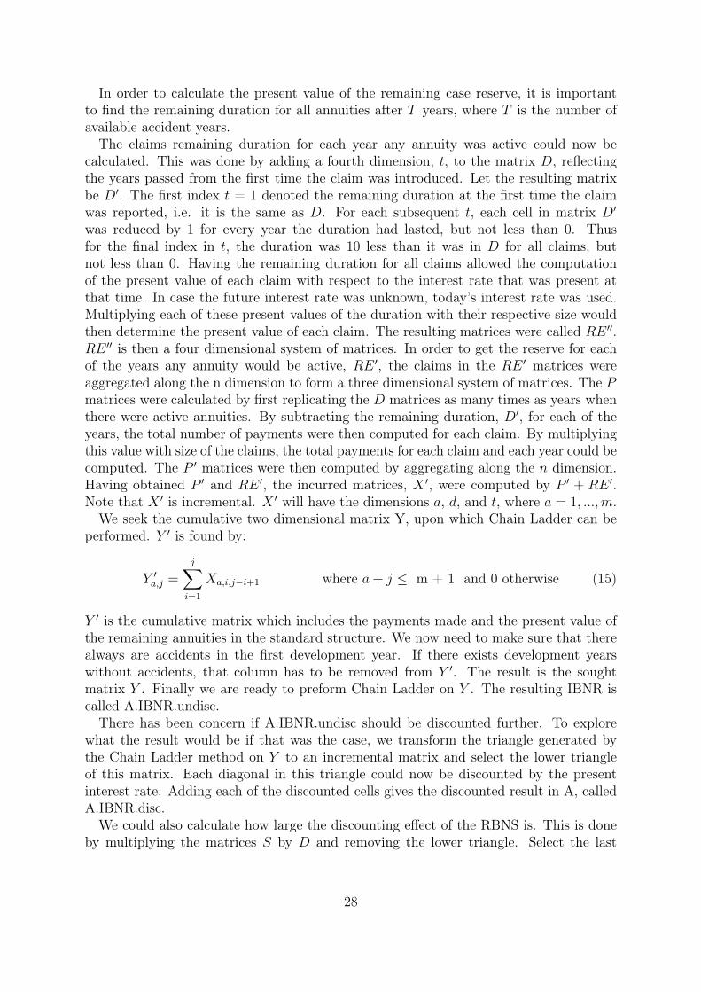
In order to calculate the present value of the remaining case reserve, it is importantto find the remaining duration for all annuities after T years, where T is the number ofavailable accident years.The claims remaining duration for each year any annuity was active could now be
calculated. This was done by adding a fourth dimension, t, to the matrix D, reflectingthe years passed from the first time the claim was introduced. Let the resulting matrixbe D′. The first index t = 1 denoted the remaining duration at the first time the claimwas reported, i.e. it is the same as D. For each subsequent t, each cell in matrix D′
was reduced by 1 for every year the duration had lasted, but not less than 0. Thusfor the final index in t, the duration was 10 less than it was in D for all claims, butnot less than 0. Having the remaining duration for all claims allowed the computationof the present value of each claim with respect to the interest rate that was present atthat time. In case the future interest rate was unknown, today’s interest rate was used.Multiplying each of these present values of the duration with their respective size wouldthen determine the present value of each claim. The resulting matrices were called RE ′′.RE ′′ is then a four dimensional system of matrices. In order to get the reserve for eachof the years any annuity would be active, RE ′, the claims in the RE ′ matrices wereaggregated along the n dimension to form a three dimensional system of matrices. The Pmatrices were calculated by first replicating the D matrices as many times as years whenthere were active annuities. By subtracting the remaining duration, D′, for each of theyears, the total number of payments were then computed for each claim. By multiplyingthis value with size of the claims, the total payments for each claim and each year could becomputed. The P ′ matrices were then computed by aggregating along the n dimension.Having obtained P ′ and RE ′, the incurred matrices, X ′, were computed by P ′ + RE ′.Note that X ′ is incremental. X ′ will have the dimensions a, d, and t, where a = 1, ...,m.We seek the cumulative two dimensional matrix Y, upon which Chain Ladder can be
performed. Y ′ is found by:
Y ′a,j =
j∑i=1
Xa,i,j−i+1 where a+ j ≤ m + 1 and 0 otherwise (15)
Y ′ is the cumulative matrix which includes the payments made and the present value ofthe remaining annuities in the standard structure. We now need to make sure that therealways are accidents in the first development year. If there exists development yearswithout accidents, that column has to be removed from Y ′. The result is the soughtmatrix Y . Finally we are ready to preform Chain Ladder on Y . The resulting IBNR iscalled A.IBNR.undisc.There has been concern if A.IBNR.undisc should be discounted further. To explore
what the result would be if that was the case, we transform the triangle generated bythe Chain Ladder method on Y to an incremental matrix and select the lower triangleof this matrix. Each diagonal in this triangle could now be discounted by the presentinterest rate. Adding each of the discounted cells gives the discounted result in A, calledA.IBNR.disc.We could also calculate how large the discounting effect of the RBNS is. This is done
by multiplying the matrices S by D and removing the lower triangle. Select the last
28
diagonal. The difference between this diagonal and the last diagonal in A.cum_knownis the discounting effect of the RBNS. Let this be called A.disc.effect.Since the A.IBNR.undisc projects the total payments, rather than the total reserve,
A.IBNR.undisc does not account for the discounting effect of the reserve. A.IBNR isobtained by removing the discounting effect, A.disc.effect, from A.IBNR.undisc.
3.4.2 Detailed Description of How Method B Was Implemented
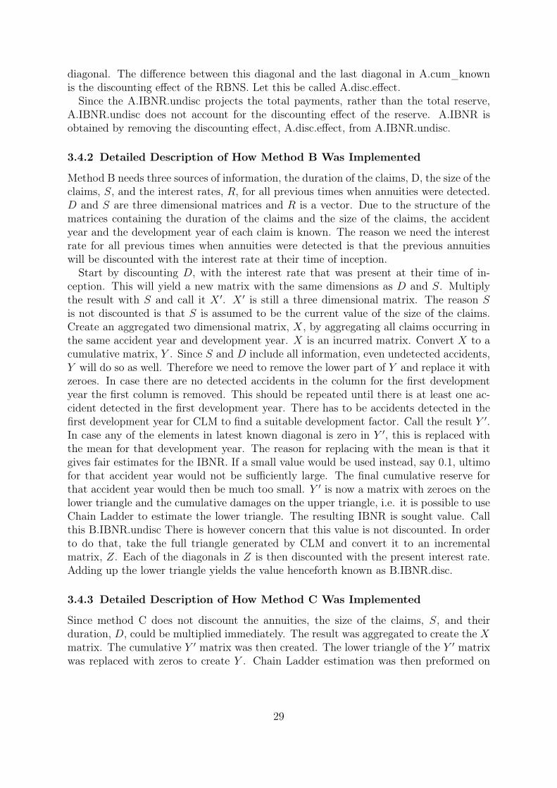
Method B needs three sources of information, the duration of the claims, D, the size of theclaims, S, and the interest rates, R, for all previous times when annuities were detected.D and S are three dimensional matrices and R is a vector. Due to the structure of thematrices containing the duration of the claims and the size of the claims, the accidentyear and the development year of each claim is known. The reason we need the interestrate for all previous times when annuities were detected is that the previous annuitieswill be discounted with the interest rate at their time of inception.Start by discounting D, with the interest rate that was present at their time of in-
ception. This will yield a new matrix with the same dimensions as D and S. Multiplythe result with S and call it X ′. X ′ is still a three dimensional matrix. The reason Sis not discounted is that S is assumed to be the current value of the size of the claims.Create an aggregated two dimensional matrix, X, by aggregating all claims occurring inthe same accident year and development year. X is an incurred matrix. Convert X to acumulative matrix, Y . Since S and D include all information, even undetected accidents,Y will do so as well. Therefore we need to remove the lower part of Y and replace it withzeroes. In case there are no detected accidents in the column for the first developmentyear the first column is removed. This should be repeated until there is at least one ac-cident detected in the first development year. There has to be accidents detected in thefirst development year for CLM to find a suitable development factor. Call the result Y ′.In case any of the elements in latest known diagonal is zero in Y ′, this is replaced withthe mean for that development year. The reason for replacing with the mean is that itgives fair estimates for the IBNR. If a small value would be used instead, say 0.1, ultimofor that accident year would not be sufficiently large. The final cumulative reserve forthat accident year would then be much too small. Y ′ is now a matrix with zeroes on thelower triangle and the cumulative damages on the upper triangle, i.e. it is possible to useChain Ladder to estimate the lower triangle. The resulting IBNR is sought value. Callthis B.IBNR.undisc There is however concern that this value is not discounted. In orderto do that, take the full triangle generated by CLM and convert it to an incrementalmatrix, Z. Each of the diagonals in Z is then discounted with the present interest rate.Adding up the lower triangle yields the value henceforth known as B.IBNR.disc.
3.4.3 Detailed Description of How Method C Was Implemented
Since method C does not discount the annuities, the size of the claims, S, and theirduration, D, could be multiplied immediately. The result was aggregated to create the Xmatrix. The cumulative Y ′ matrix was then created. The lower triangle of the Y ′ matrixwas replaced with zeros to create Y . Chain Ladder estimation was then preformed on
29
Y . The resulting IBNR was called C.IBNR.undisc. This result is not discounted on anylevel, and does therefore overstate the reserve when interest rates are positive. In orderto take the discounting effects under consideration, the full triangle generated by CLMwas therefore converted to an incurred matrix, Z. The lower triangle of Z was discountedwith the current interest rate. Adding the discounted values of Z and multiplying by thecorrection factor, equation (14), yielded the discounted IBNR, called C.IBNR.
3.4.4 Detailed Description of How Method D Was Implemented
Method D was implemented in exactly the same way as method B, with the exceptionof the initial discounting step. Method D only uses the present interest rate to discountmatrix S, regardless of when the accidents were detected. The discounting is done in thesame manner as in method B, but this time only the present interest rate is used. Theremaining procedure does not differ from method B.
3.4.5 Adjusting method B to Present Assumptions
For companies who have stored data on theX matrix in method B, it would be interestingif there were a simple way to get a result similar to the ideal solution, method D, by asimple manipulation of the X matrix. The obvious method would be to just implementmethod D. However, if the data is hard to access for any reason, it would be useful to havea simple method of correcting the X matrix to get the desired result. We shall explorehow implementing the correction factor suggested in section 2.6.3 will affect the result.In order to use formula (13) we would need the interest rate at the time of inceptionfor all annuities and the average duration for the annuities, both historical and present.Use formula (13) for all interest rates and apply this to the corresponding cells in the Xmatrix. Then proceed as in method B. The result is called B.adjusted.
3.4.6 Detailed Description of How the True Value Was Calculated
Since all data about future payments are known in the simulations, it is possible tocalculate the exact current value of the future annuities. Consider an annuity, A, withduration d, that will be detected at t+ u. We will calculate the value of this annuity byusing the present interest rate, it, to discount the annuity by first calculating the presentvalue of the annuity using the geometric series sum. Adding all these present values givesus the value true.undisc, which corresponds to B.IBNR. However, the present values at afuture time (t+u) should be discounted to the present time, t. Thus, we should discountthese annuities with (1 + it)
u. This gives us the True Value, which is the present value ofthe future annuities.When assuming that all future information is known, it would be possible to use the
interest rates that will be present in the future. Say the present interest rate is it wherei is interest rate and t is the time. To calculate the present value an annuity that will bedetected in the future, we will discount by the present interest rate, even if we know thecorrect interest rate, it+u. Using it would yield a value a lot closer to the values calculatedby the other methods. If the interest rate present at the time the annuity is detected,it+u, would be used instead, the result would not be as interesting, since the difference
30
between the True Value and the other methods will almost always be a function of theinterest rate at it+u compared to it. By using the interest rate it we expect on averagethat the other methods will underestimate the true value 50% of the time.
3.5 Simulation
In order to prepare the simulations, we need to determine the interest rate, r, and thenumber of simulations. The number of simulations is set to 10 000.The first step in every simulation is to generate data according to the method described
in section 3.2. These matrices were then subjected to the methods described in section3.4. Each of the methods were subjected to the same data, which makes the comparisonsbetter than if data were generated separately for each method.The data will be 10 × 10 matrices.The correlation between the duration and the size of the claim is low, -0.057 with a
p-value of 0.35 according to the data. Thus we will assume that duration and size areuncorrelated. In the simulation, we will not only assume that they are uncorrelated, butalso independent. Therefore it is possible to simulate the duration and size independentseparately and combine them later.
31

4 Results from the Methods
4.1 Results from Methods A, B, C and D
The simulation results are presented in appendix A. The methods were tested by countingthe number of times the methods underestimate the IBNR relative to the True Value. Ifthe probability is 50% to underestimate the True Value and 10 000 simulations are made,we can use an exact binomial test with a 95% confidence interval to find the number oftimes the methods should underestimate the true IBNR. According to the exact binomialtest, a method with a 50% chance to underestimate the IBNR will underestimate theIBNR between 4901 and 5099 times in 95% of the simulations. Note that this confidenceinterval is not adjusted for the number of tests. A high number of tests should have awider confidence interval.The figures below are separated into two parts. The left part shows the difference
between each method and the true value in a step graph. The right part shows a boxplot with the same values.
4.1.1 Results with Zero Interest Rates
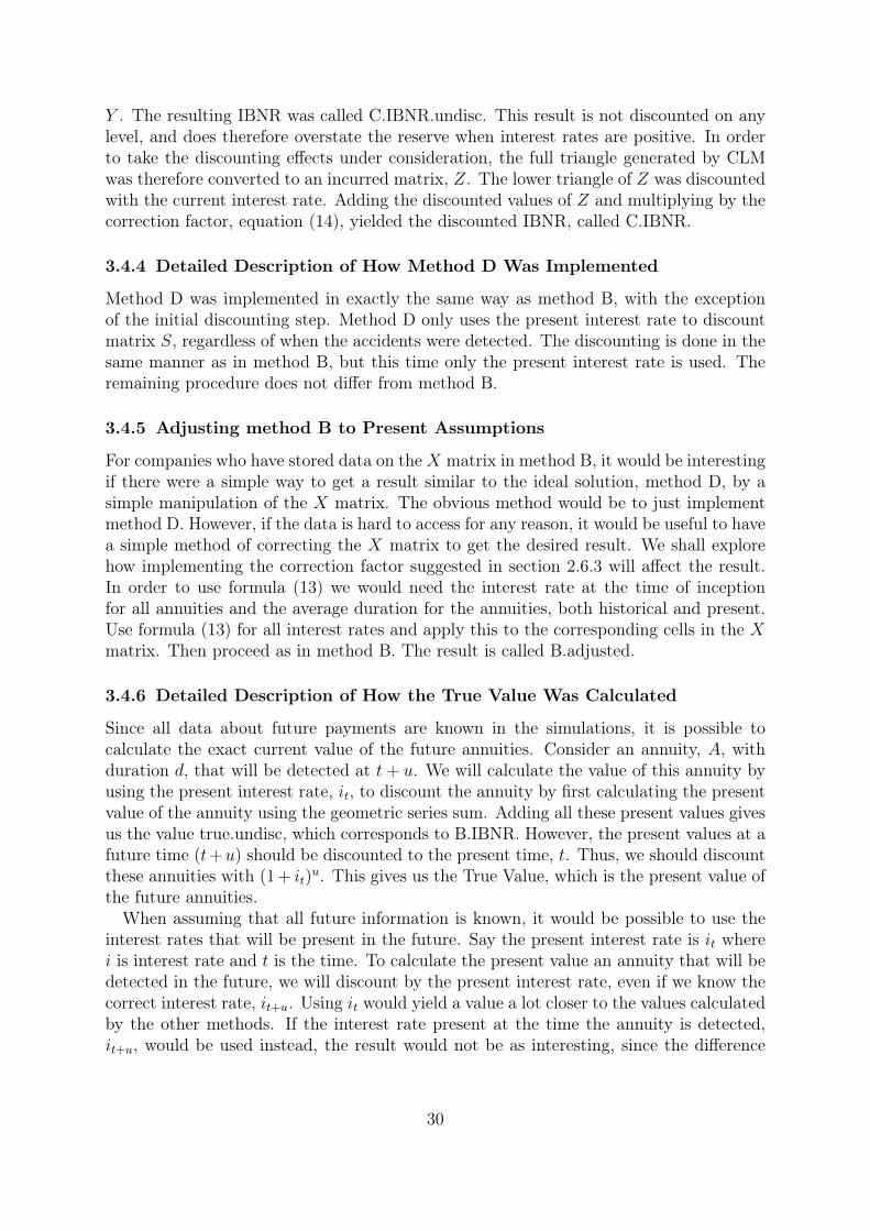
The results from the simulations with zero interest rate is presented in table 11 and figure1.A, B, B’, C and D were all equal. The difference between the True Value and the group
with A, B, B’, C and D was very small.The True Value uses future information, but the other methods only use information
available at the present time. The result of expected claims versus the actual claims willbe similar, but not identical. Table 11 in appendix A shows that the difference betweenthe actual and the estimated IBNR is less than 1% on average.The fact that the results between the estimated and the True IBNR are similar indicates
that the methods are correctly implemented.All the estimated IBNR were equal when the interest rate was zero, which implies that
differences between the methods in the simulations when the interest rates were not zero,were caused by interest rates.The estimated IBNR was smaller than the True Value 4987 times in 10 000 simulations
for all methods, well inside the 95% confidence interval. This indicates that all methodsare suitable when the interest rate is zero.
32
Figure 1: Results with Zero interest rates. The left graph shows the distribution of thedifference between the reserves estimated by the methods and the true value.When the interest rate is 0, all methods generate the same result. All linesoverlap. The right graph shows a box plot of the same values for each of themethods.
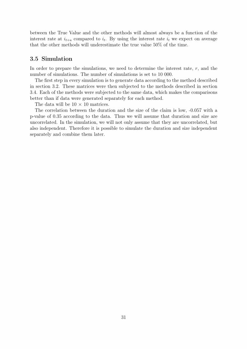
4.1.2 Results with Fixed Positive Interest Rates
The results from the simulations with fixed positive interest rates are presented in table12, 13 and 14 and figure 2, 3 and 4.When the interest rate is fixed, method B, B’ and D are identical, since the present
interest rate is the same as the historical interest rate. The three methods mentionedpreform well under these circumstances. After 10 000 simulations, the mean of thesemethods are less than 1% different from the mean of the True Method. C was veryclose, but not identical, to the previously described methods. The four methods, B, B’,C and D, slightly overestimate the IBNR in all the three cases when the interest ratewas positive, but the differences are not minuscule. In all cases it is slightly more likelythat the methods underestimated IBNR in a specific simulation. Both with 2% and 4%interest rate, the number of simulations that underestimated the IBNR was well insidethe confidence interval, which had an upper limit of 50.99%. When the interest rate was8% the B and D were slightly outside of the confidence interval, but remember that theconfidence interval was constructed for a single test and not adjusted for the high numberof tests performed here. Method C was on par with the B, B’ and D.Method A overestimated the IBNR in most cases and performed worse than all other
33
Figure 2: Results with 2% interest rates. The left graph shows the distribution of thedifference between the reserves estimated by the methods and the true value.The weak dotted line represents method A. The other lines overlap. The rightgraph shows a box plot of the same values for each of the methods.
methods.
34
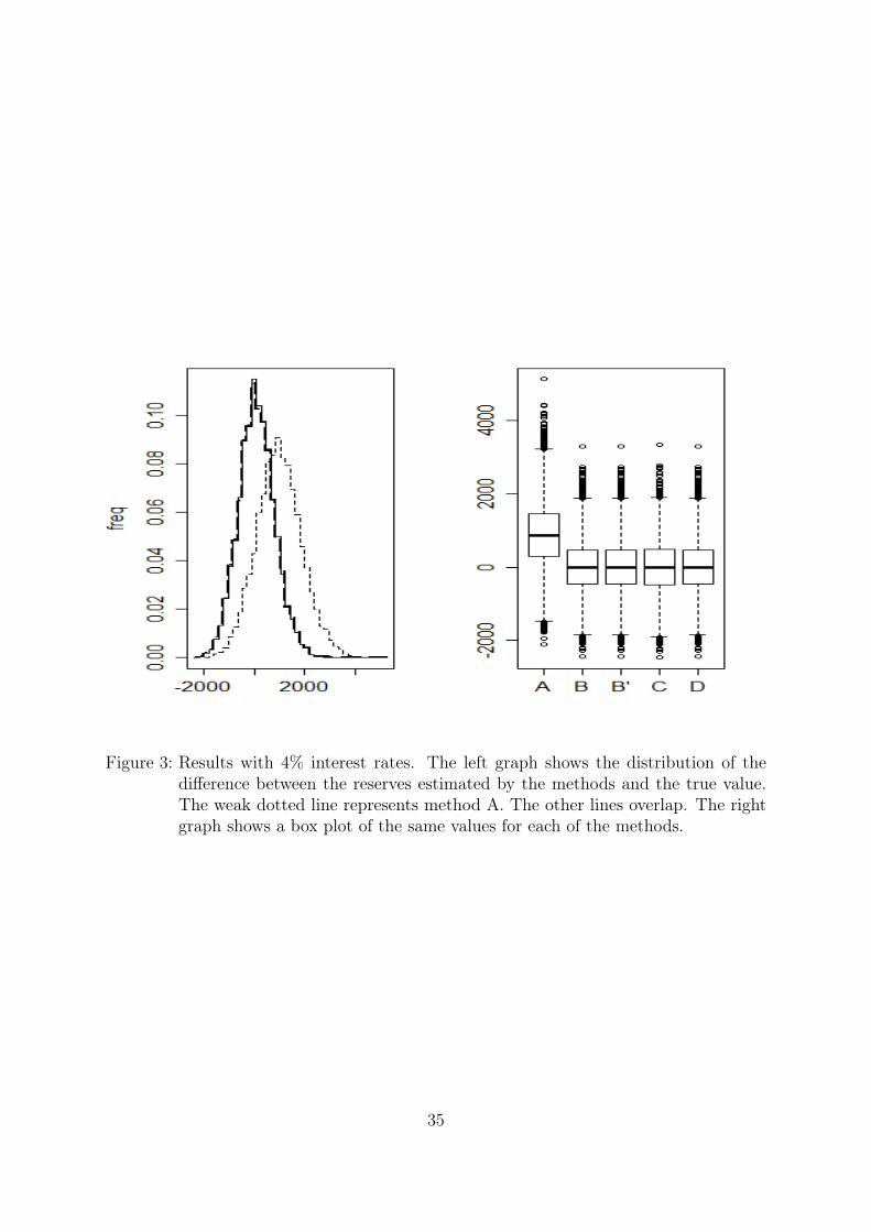
Figure 3: Results with 4% interest rates. The left graph shows the distribution of thedifference between the reserves estimated by the methods and the true value.The weak dotted line represents method A. The other lines overlap. The rightgraph shows a box plot of the same values for each of the methods.
35
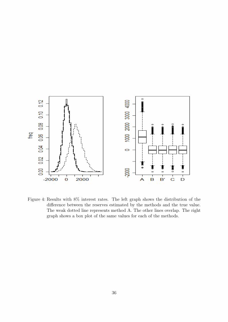
Figure 4: Results with 8% interest rates. The left graph shows the distribution of thedifference between the reserves estimated by the methods and the true value.The weak dotted line represents method A. The other lines overlap. The rightgraph shows a box plot of the same values for each of the methods.
36

4.1.3 Results with Fixed Negative Interest Rates
The results from the simulations with fixed negative interest rates are presented in table15 to 17 and figures 5 to 7.As in the previous cases with a fixed, positive interest rate, the methods B, B’ and
D are identical when the interest rate is fixed and negative. The effects with negativeinterest rates are mirroring the previous results with positive interest rates. B, B’ C andD still produce good results with small errors. Method A does not change enough andwill underestimate the IBNR.
Figure 5: Results with -2% interest rates. The left graph shows the distribution of thedifference between the reserves estimated by the methods and the true value.The solid line represents method A. The other lines overlap. The right graphshows a box plot of the same values for each of the methods.
37
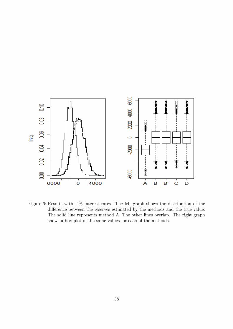
Figure 6: Results with -4% interest rates. The left graph shows the distribution of thedifference between the reserves estimated by the methods and the true value.The solid line represents method A. The other lines overlap. The right graphshows a box plot of the same values for each of the methods.
38

Figure 7: Results with -8% interest rates. The left graph shows the distribution of thedifference between the reserves estimated by the methods and the true value.The solid line represents method A. The other lines overlap. The right graphshows a box plot of the same values for each of the methods.
39
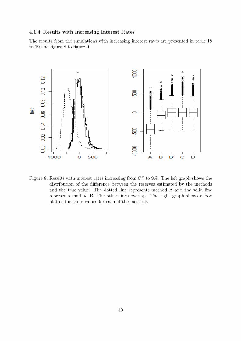
4.1.4 Results with Increasing Interest Rates
The results from the simulations with increasing interest rates are presented in table 18to 19 and figure 8 to figure 9.
Figure 8: Results with interest rates increasing from 0% to 9%. The left graph shows thedistribution of the difference between the reserves estimated by the methodsand the true value. The dotted line represents method A and the solid linerepresents method B. The other lines overlap. The right graph shows a boxplot of the same values for each of the methods.
40
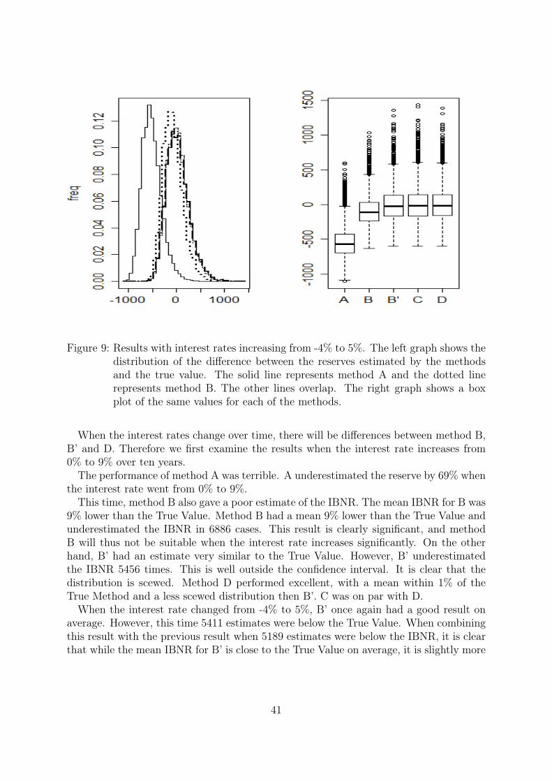
Figure 9: Results with interest rates increasing from -4% to 5%. The left graph shows thedistribution of the difference between the reserves estimated by the methodsand the true value. The solid line represents method A and the dotted linerepresents method B. The other lines overlap. The right graph shows a boxplot of the same values for each of the methods.
When the interest rates change over time, there will be differences between method B,B’ and D. Therefore we first examine the results when the interest rate increases from0% to 9% over ten years.The performance of method A was terrible. A underestimated the reserve by 69% when
the interest rate went from 0% to 9%.This time, method B also gave a poor estimate of the IBNR. The mean IBNR for B was
9% lower than the True Value. Method B had a mean 9% lower than the True Value andunderestimated the IBNR in 6886 cases. This result is clearly significant, and methodB will thus not be suitable when the interest rate increases significantly. On the otherhand, B’ had an estimate very similar to the True Value. However, B’ underestimatedthe IBNR 5456 times. This is well outside the confidence interval. It is clear that thedistribution is scewed. Method D performed excellent, with a mean within 1% of theTrue Method and a less scewed distribution then B’. C was on par with D.When the interest rate changed from -4% to 5%, B’ once again had a good result on
average. However, this time 5411 estimates were below the True Value. When combiningthis result with the previous result when 5189 estimates were below the IBNR, it is clearthat while the mean IBNR for B’ is close to the True Value on average, it is slightly more
41
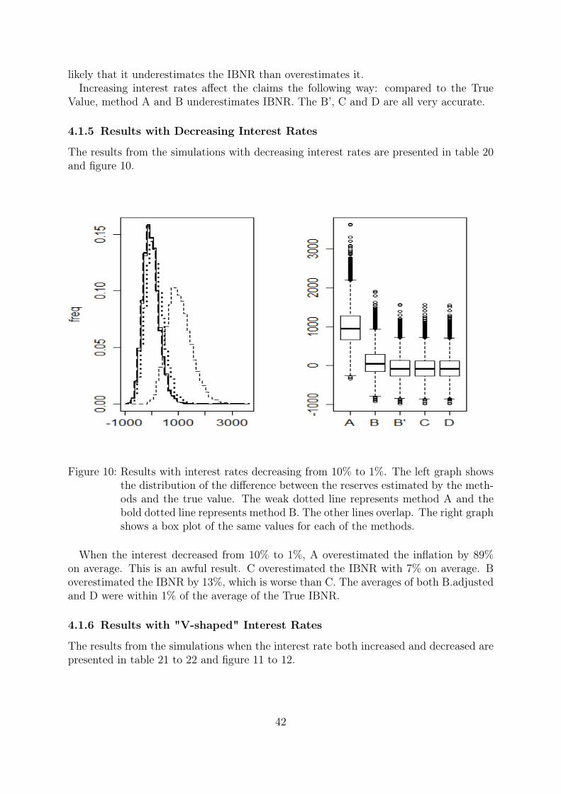
likely that it underestimates the IBNR than overestimates it.Increasing interest rates affect the claims the following way: compared to the True
Value, method A and B underestimates IBNR. The B’, C and D are all very accurate.
4.1.5 Results with Decreasing Interest Rates
The results from the simulations with decreasing interest rates are presented in table 20and figure 10.
Figure 10: Results with interest rates decreasing from 10% to 1%. The left graph showsthe distribution of the difference between the reserves estimated by the meth-ods and the true value. The weak dotted line represents method A and thebold dotted line represents method B. The other lines overlap. The right graphshows a box plot of the same values for each of the methods.
When the interest decreased from 10% to 1%, A overestimated the inflation by 89%on average. This is an awful result. C overestimated the IBNR with 7% on average. Boverestimated the IBNR by 13%, which is worse than C. The averages of both B.adjustedand D were within 1% of the average of the True IBNR.
4.1.6 Results with "V-shaped" Interest Rates
The results from the simulations when the interest rate both increased and decreased arepresented in table 21 to 22 and figure 11 to 12.
42
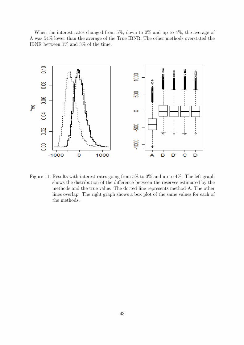
When the interest rates changed from 5%, down to 0% and up to 4%, the average ofA was 54% lower than the average of the True IBNR. The other methods overstated theIBNR between 1% and 3% of the time.
Figure 11: Results with interest rates going from 5% to 0% and up to 4%. The left graphshows the distribution of the difference between the reserves estimated by themethods and the true value. The dotted line represents method A. The otherlines overlap. The right graph shows a box plot of the same values for each ofthe methods.
43
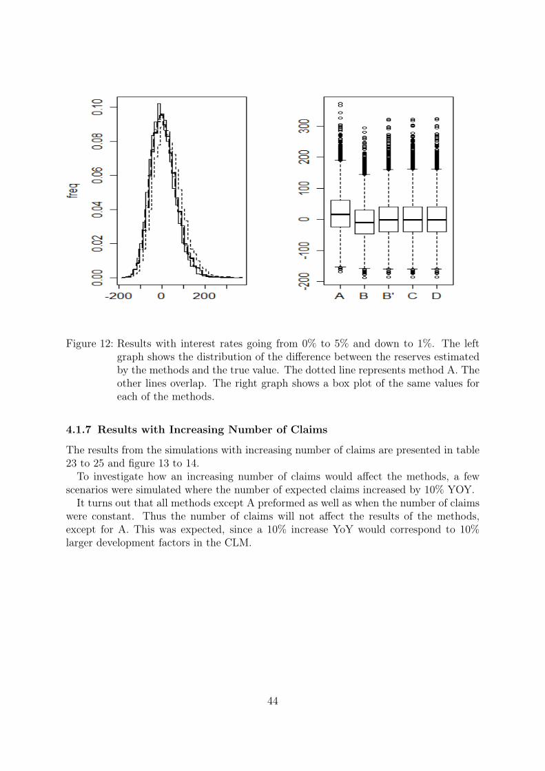
Figure 12: Results with interest rates going from 0% to 5% and down to 1%. The leftgraph shows the distribution of the difference between the reserves estimatedby the methods and the true value. The dotted line represents method A. Theother lines overlap. The right graph shows a box plot of the same values foreach of the methods.
4.1.7 Results with Increasing Number of Claims
The results from the simulations with increasing number of claims are presented in table23 to 25 and figure 13 to 14.To investigate how an increasing number of claims would affect the methods, a few
scenarios were simulated where the number of expected claims increased by 10% YOY.It turns out that all methods except A preformed as well as when the number of claims
were constant. Thus the number of claims will not affect the results of the methods,except for A. This was expected, since a 10% increase YoY would correspond to 10%larger development factors in the CLM.
44
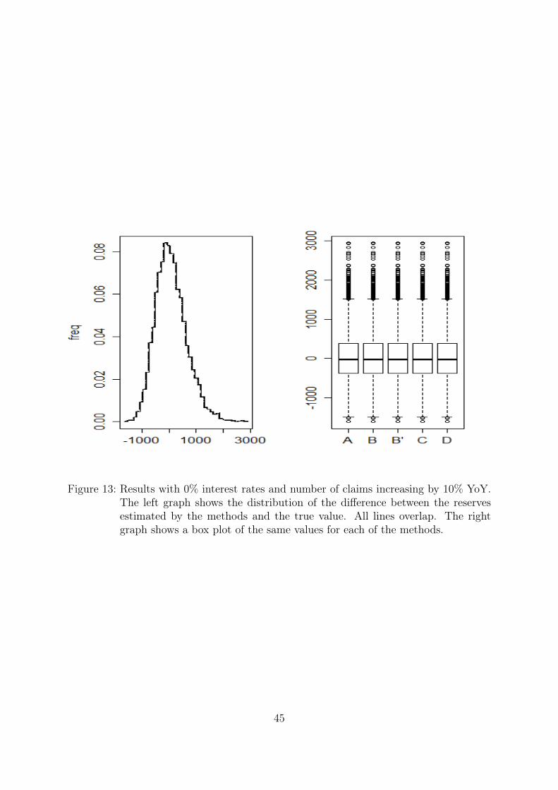
Figure 13: Results with 0% interest rates and number of claims increasing by 10% YoY.The left graph shows the distribution of the difference between the reservesestimated by the methods and the true value. All lines overlap. The rightgraph shows a box plot of the same values for each of the methods.
45
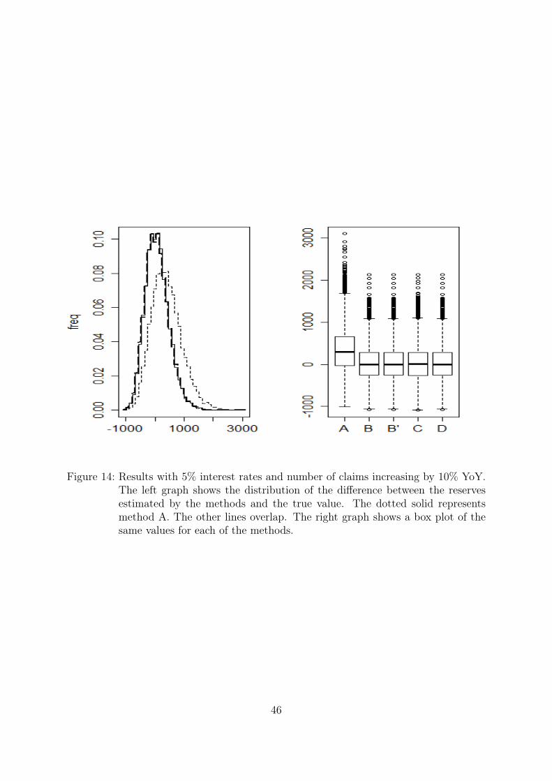
Figure 14: Results with 5% interest rates and number of claims increasing by 10% YoY.The left graph shows the distribution of the difference between the reservesestimated by the methods and the true value. The dotted solid representsmethod A. The other lines overlap. The right graph shows a box plot of thesame values for each of the methods.
46
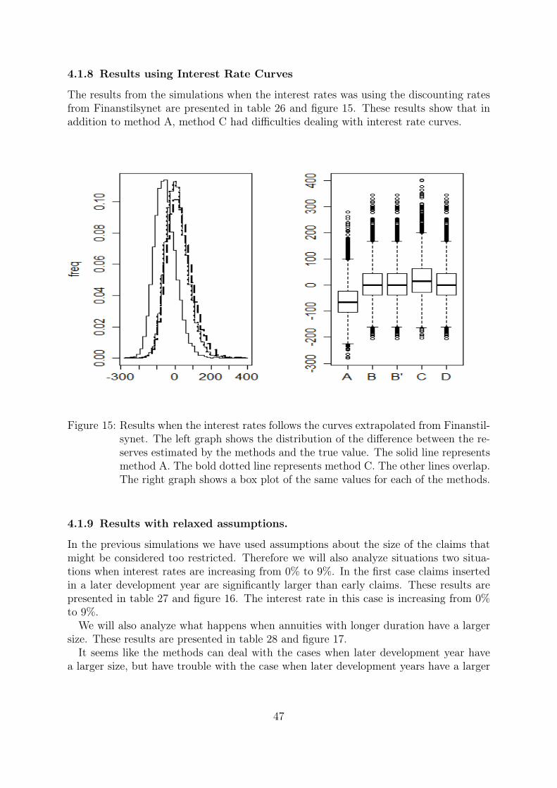
4.1.8 Results using Interest Rate Curves
The results from the simulations when the interest rates was using the discounting ratesfrom Finanstilsynet are presented in table 26 and figure 15. These results show that inaddition to method A, method C had difficulties dealing with interest rate curves.
Figure 15: Results when the interest rates follows the curves extrapolated from Finanstil-synet. The left graph shows the distribution of the difference between the re-serves estimated by the methods and the true value. The solid line representsmethod A. The bold dotted line represents method C. The other lines overlap.The right graph shows a box plot of the same values for each of the methods.
4.1.9 Results with relaxed assumptions.
In the previous simulations we have used assumptions about the size of the claims thatmight be considered too restricted. Therefore we will also analyze situations two situa-tions when interest rates are increasing from 0% to 9%. In the first case claims insertedin a later development year are significantly larger than early claims. These results arepresented in table 27 and figure 16. The interest rate in this case is increasing from 0%to 9%.We will also analyze what happens when annuities with longer duration have a larger
size. These results are presented in table 28 and figure 17.It seems like the methods can deal with the cases when later development year have
a larger size, but have trouble with the case when later development years have a larger
47
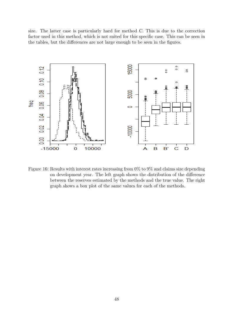
size. The latter case is particularly hard for method C. This is due to the correctionfactor used in this method, which is not suited for this specific case. This can be seen inthe tables, but the differences are not large enough to be seen in the figures.
Figure 16: Results with interest rates increasing from 0% to 9% and claims size dependingon development year. The left graph shows the distribution of the differencebetween the reserves estimated by the methods and the true value. The rightgraph shows a box plot of the same values for each of the methods.
48
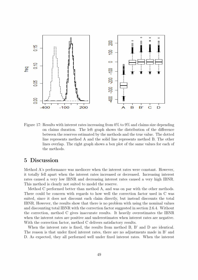
Figure 17: Results with interest rates increasing from 0% to 9% and claims size dependingon claims duration. The left graph shows the distribution of the differencebetween the reserves estimated by the methods and the true value. The dottedline represents method A and the solid line represents method B. The otherlines overlap. The right graph shows a box plot of the same values for each ofthe methods.
5 DiscussionMethod A’s performance was mediocre when the interest rates were constant. However,it totally fell apart when the interest rates increased or decreased. Increasing interestrates caused a very low IBNR and decreasing interest rates caused a very high IBNR.This method is clearly not suited to model the reserve.Method C performed better than method A, and was on par with the other methods.
There could be concern with regards to how well the correction factor used in C wassuited, since it does not discount each claim directly, but instead discounts the totalIBNR. However, the results show that there is no problem with using the nominal valuesand discounting total IBNR with the correction factor suggested in section 2.6.4. Withoutthe correction, method C gives inaccurate results. It heavily overestimates the IBNRwhen the interest rates are positive and underestimates when interest rates are negative.With the correction factor, method C delivers satisfactory results.When the interest rate is fixed, the results from method B, B’ and D are identical.
The reason is that under fixed interest rates, there are no adjustments made in B’ andD. As expected, they all performed well under fixed interest rates. When the interest
49
rate changed, the performance of method B declined. Increasing interest rates causes Bto underestimate the IBNR and vice versa. Both B’ and D still did well. The differencebetween B’ and D was very small, much smaller than the author had expected. Thisindicates that the correction suggested in section 2.6.3 is well suited to adjust the datato the current interest rate.One thing to note about the number of times the methods underestimated the True
IBNR is that although method B and D were well inside the confidence interval in mostcases, they only underestimated the True IBNR once each in 15 simulations. This ishighly significant. These methods are more likely to overestimate than underestimatethe IBNR. Note that although it is more likely that the IBNR will be underestimated,the probability is only slightly more than 50%.Method D does not seem to be a significant improvement over B’. Therefore, if a
company would already have stored the data in the form used for B, the adjustmentsuggested in section 2.6.3 would be enough to account for the difference in interest rate.
5.1 Recommendations
The results with using the case reserves as basis for the IBNR calculations, as in methodA, were not good. Unfortunately, we cannot recommend using this method. Despite theallure of using the easily accessible case reserves, the results from this study shows thatthis method is too unreliable.Method B has the advantage for the actuary that he does not have to update the
triangles with regards to new interest rates. This method is suitable when the interestrate is constant or changing very little. Its worst performance is when the interest rates arestrictly increasing or decreasing for the entire period. If the interest rates are fluctuatingback and forth, the changes are not that large compared to the other methods. If thedata already is as in B, and the actuary is concerned about the effects of the interestrates, it is possible to make the relatively simple adjustment suggested in section 2.6.3.This will cause the effects of the change of the interest rates to be minimized.Method C has the obvious advantage that no discounting is done in the initial step.
Therefore, like in method B, there is no need to update the past claims in the triangles.The differences between the past and the present interest rates can be found by simplyadjusting the IBNR directly. This should have some appeal since one does not have toredo old calculations. However, the actuary would need access to the duration of all claimsin order to discount properly. This might cause problems if the actuary is working on anaggregate level when doing the reserving and has trouble retrieving that data afterwards.Method D has the advantage that the correct discounting is used all the time. The dis-
advantage is that the actuary has to keep track of all previous claims on an undiscountedlevel and update the triangle every time the reserve should be calculated. The resultswith this method are good, just as one would have predicted. There are no correctionfactors needed in order to find the best estimate.Table 10 summarizes the results.
50
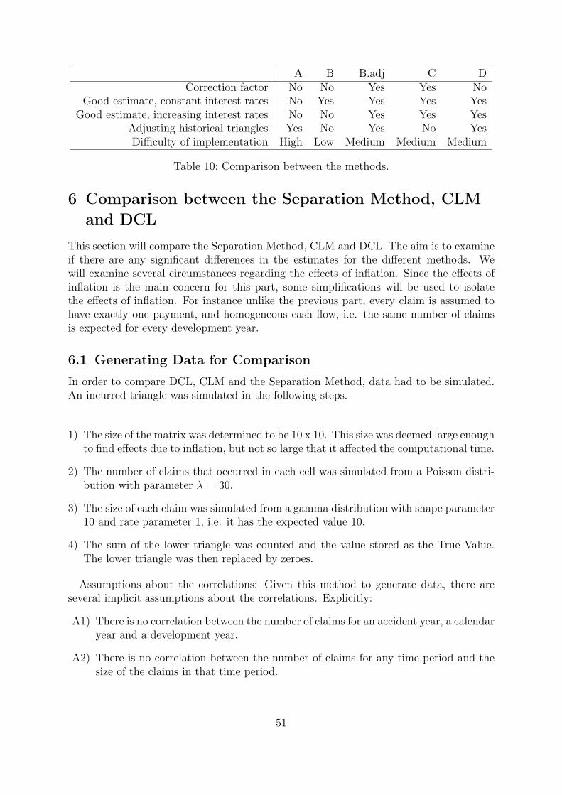
A B B.adj C DCorrection factor No No Yes Yes No
Good estimate, constant interest rates No Yes Yes Yes YesGood estimate, increasing interest rates No No Yes Yes Yes
Adjusting historical triangles Yes No Yes No YesDifficulty of implementation High Low Medium Medium Medium
Table 10: Comparison between the methods.
6 Comparison between the Separation Method, CLMand DCL
This section will compare the Separation Method, CLM and DCL. The aim is to examineif there are any significant differences in the estimates for the different methods. Wewill examine several circumstances regarding the effects of inflation. Since the effects ofinflation is the main concern for this part, some simplifications will be used to isolatethe effects of inflation. For instance unlike the previous part, every claim is assumed tohave exactly one payment, and homogeneous cash flow, i.e. the same number of claimsis expected for every development year.
6.1 Generating Data for Comparison
In order to compare DCL, CLM and the Separation Method, data had to be simulated.An incurred triangle was simulated in the following steps.
1) The size of the matrix was determined to be 10 x 10. This size was deemed large enoughto find effects due to inflation, but not so large that it affected the computational time.
2) The number of claims that occurred in each cell was simulated from a Poisson distri-bution with parameter λ = 30.
3) The size of each claim was simulated from a gamma distribution with shape parameter10 and rate parameter 1, i.e. it has the expected value 10.
4) The sum of the lower triangle was counted and the value stored as the True Value.The lower triangle was then replaced by zeroes.
Assumptions about the correlations: Given this method to generate data, there areseveral implicit assumptions about the correlations. Explicitly:
A1) There is no correlation between the number of claims for an accident year, a calendaryear and a development year.
A2) There is no correlation between the number of claims for any time period and thesize of the claims in that time period.
51
A3) There is no correlation between the delay and the size of the claims, when theinflation effect is discounted.
Note: If the inflation is set to 0, the expected value the lower triangle is easy to calcu-late. There are 45 unknown cells. Since the cash flow is homogeneous, each cell has thirtyexpected claims. Each claim is expected to be of size 10. Thus the expected IBNR isE[Size of the claim] × E[Number of claims] × (Number of cells) = 10 × 30 × 45 = 13 500.
The upper triangle generated this way was subject to the three methods, DCL, CLMand Separation Method, for estimating the reserve. The different values for each accidentyear will not be considered, only the total outstanding payments are taken into account.The reason for simplifying the process this way is that it is more meaningful to comparedata on this level when comparing the methods. Doing it for every accident year givesmuch more data, but it is not clear how it would improve the comparisons. The processof generating data was then repeated 10 000 times to give an accurate estimate of thedifferences between the methods under different scenarios.
6.2 The True IBNR
Given the way the data is simulated it is possible to know the full matrix, not onlythe upper triangle. For any meaningful comparison between different methods the lowertriangle has to be replaced with zeroes when estimating the reserve with different methods.However, the lower triangle is the ideal estimate, i.e. the result generated by a perfectmethod. Thus the True IBNR is just the sum the lower triangle. This differs fromthe True Value used to compare the annuity methods since it is not discounted. It wascalculated as a reference to see how well the methods preformed. The relative value ofthe True IBNR and the different methods could therefore be examined. A perfect resultwould have a relative value of 1. It would never be possible to consistently get a relativevalue of one, since the future claims are stochastic. However, the mean of the relativevalue should be close to one.
6.3 Results from the Simulation
The results from the simulations are presented in in tables in Appendix B. To comparethe results we examine how different inflation rates affect the methods. The results forall the scenarios tested show that the three methods have a very similar result for all thetested scenarios. Appendix C presents graphs from the results of CLM, DCL and theSeparation Method when the simulated true value for each simulation has been subtractedfrom each estimate.
6.3.1 Zero Inflation, Constant Number of Claims
To establish a baseline for the methods, we start by examining how the methods comparewithout inflation present. As shown in Appendix B and C, the three methods have verysimilar distributions, but the True Method stands out. As expected, the distributions all
52
look like normal distributions. There is very little difference between the methods withzero inflation. This indicates that they are all equally well suited for estimating IBNRwhen inflation is not present.Although the methods are very similar, it should be noted that the DCL seems to have
a closer fit than the other methods. However, the mean of DCL is the largest one. Thedifference is 2% after 10 000 simulations. We would expect the mean of CLM to be veryclose to the mean of the True Method, since CLM is unbiased. The Separation Methodhad an even closer fit. This was somewhat surprising, since the Separation Method is notunbiased.Are the methods equally likely to over- or underestimate? Despite the fact that the
mean for the DCL is larger than for the other methods, it is not clear if the reason is thatthere are a few large values that drive up the average or if it is biased. It is possible to use asign test to examine if the methods over- or underestimate equal number of times. Countthe number of times each method gives an estimate smaller than the True estimate. Outof the 10 000 simulations, the CLM underestimated 4907 times, the Separation Method4964 times and DCL 4592 times. An exact binomial test states that the p-values are6.4%, 47.8% and 3.5 · 10−16 respectively. Thus it is clear that the DCL does overestimatethe IBNR most of the time.We could also examine the relative accuracy of the methods. Take the estimate pro-
vided by a specific method and divide by the True Method. The 2.5% and 97.5% percentileare then CLM (0.78, 1.28), DCL (0.81, 1.29), SM (0.79, 1.26). It could be noted thatthe interval for DCL is slightly tighter than CLM, despite having a higher estimate onaverage. SM had the tightest interval of the three methods.
It is noteworthy that the True IBNR has a significantly smaller variance than the othermethods. This is not surprising. The variance in the true value is only the result of vari-ance in the process for generating claims. The other methods will be subjected to thisvariance in addition to the errors in estimation process.
6.3.2 Constant High Inflation, Constant Number of Claims
If the inflation is high, but constant, there might be concerns that there could be adifference between the methods. Here the inflation is 10% per year. As can be seen inthe figure in appendix C, again there is very little difference between the methods.
6.3.3 Other Results
Many other scenarios were tested where inflation, interest rate and the number of claimschanged in various ways. Some of those results are presented in Appendix B and C. Asit turns out, regardless of the changes, there were few differences between the methods.
53
6.4 Comments about the Methods
One disadvantage with DCL is that it does not always work well for all data sets. If theinflation of the claims is not large enough, two things will cause trouble.
1) The estimate for the delay parameter becomes hard to obtain. The delay functionshould not have any negative numbers. However, it can happen when the inflation isnot large enough.
2) It fails to calculate the variance of the individual size of claims. The way the variance iscalculated in the article by Martinez - Miranda, et. al (2012), it can become negative.This does not influence the estimated IBNR. However, if DCL would be used to forbootstrapping purposes, a negative variance estimate would cause severe problems.
These problems are known and mentioned in the paper by Martinez - Miranda, et. al(2012).DCL’s ability to estimate the variance of the individual claims’ size will depend on the
number of claims each year and the size of the inflation. If the inflation would only affectthe claims on an accident year basis, it would not influence DCL’s ability to estimate thevariance.In the paper by Martinez - Miranda, et al. (2012). DCL was designed to work on
payments, rather than on incurred claims. The decision for using payments rather thanincurred data was likely based on the same arguments as in Verrall, et al. (2010). Thereasons stated in that paper are that only using payments does not involve any humanjudgment. The estimates and the actual payments often differ. There could be politicaland business related considerations which might make the data unreliable. Some varianceis also avoided, since the estimates are often inaccurate. The final reason stated in thatpaper is that cash flow modeling can be disrupted as claims estimates appear as paid atthe wrong point in time. This becomes troublesome when considering annuities. Usingthe payments of the annuities rather than the incurred claims often causes the estimatedclaims, X, to be negative. The estimate of the IBNR also becomes unrealistic. Therefore,it is better to consider the incurred claims rather than the payments in the DCL whenmodeling annuities.We expect that CLM will generate a relatively good result on average, since CLM is
unbiased. What would be interesting to know, is how the results differed from the TrueValue on average under certain constraints. The Separation Method is not unbiased. Itwould be useful to be able to make generalizations about how the Separation Methodestimates the claims and in which direction based on the inflation. Is the result dependenton the inflation or does it always over- or underestimate the IBNR? Would a negativeinflation make the result different? Generalizations based on simple, known factors likethese could be useful.As it turns out, the choice of method had little effect on the results. The most noticeable
difference was in the extreme cases when the methods had a large discrepancy with thetrue result. The Separation Method was less likely to overestimate the result heavily andDCL was less likely to underestimate heavily. This result was surprising to the author. Allsources referred to in chapter 2.4.1 and 2.4.2 called for caution when using CLM under
54

changing inflation and warned that the Separation Method might be unstable. Theseresults indicate that under the examined circumstances, it is rare that the choice ofmethod has a large impact. This might be due to the assumptions made when simulatingthe methods. As a test, we also tried an extreme case using a log-normal distributionwith parameters mean ln(1) and variance ln(1.5). To further distort the data, the claimsin the first two development years were ten times larger than the following developmentyears. Finally the number of claims expected to be detected in each development yearfollowed the distribution used in the section 3.3. This result is shown in appendix B,table 34 and appendix C figure 23. From the result, it is clear that under these extremecircumstances, DCL was much worse than the other methods. The Separation Methodwas better than CLM. Therefore, it seems reasonable to conclude that the similarities inthe previous results might be a consequence of the assumptions in section 6.1 being tooadjusted.
55
7 References
7.1 Litterature
Aït-Sahalia, Y. (1996) Testing Continuous-Time Models of the Spot Interest RatesReview of Financial Studies, 9, 385-426.
Atkinson, R. (1989) Calculating IBNR Based on Case Reserves Casualty ActuarialSociety Forum, Fall, 1989, 39-44
Björk,T. (2009) Arbitrage Theory in Continuous Time. Oxford University Press.302-315
Björkwall, S. (2011) Stochastic claims reserving in non-life insurance. Departmentof Mathematics, Stockholm University
Brickman, S., Foster, W., Sheaf, S., (2005) Claims Inflation - Uses and Abuses.GIRO Conference, http://www.actuaries.org.uk
Cox, J.C., Ingersoll, J.E., and Ross, S.A. (1985) A Theory of the Term Structureof Interest Rates Econometrica 53, 384-406
Dahl, P. (2014) Introduction to Reserving.kurser.math.su.se/mod/resource/view.php?id=9921
Carrato, A., Concina, F., Gesmann, M., Murphy, D., Wüthrich, M. andWayne, Z. (2015) R-package "Chain-Ladder" version 0.2.2 (31 August, 2015) URL:https://github.com/mages/ChainLadder#chainladder
Martinez Miranda, M. Nielsen, J.P. and Verrall, R. (2012) Double ChainLadder. ASTIN Bulletin 40(1), 59-76
Mack, T., (1993) Distribution-free Calculation of the Standard Error of Chain LadderReserve Estimates. ASTIN Bulletin, Vol. 23, No. 2, 213-225
Norberg, R. (1986) A Contribution to Modelling of IBNR Claims. ScandinavianActuarial Journal, 3, 155-203
R Development Core Team (2011), R: A Language and Environment for StatisticalComputing. Vienna, Austria : the R Foundation for Statistical Computing. ISBN: 3-900051-07-0. URL: www.R-project.org/
Taylor, G. Loss Reserving. (2000) An Actuarial Perspective Kluwer Academic Pub-lishers
56
Taylor, G. C., (1977) Separation of Inflation and other Effects from the Distributionof Non-Life Insurance Claim Delays. ASTIN Bulletin, 9, 219-2300
Verrall, R., Nielsen, J.P., and Jessen, A. (2010) Including Count Data in ClaimsReserving. ASTIN Bulletin 40(2), 871-887
Wütrich, M.V. and Merz, M. (2008) Stochastic Claims Reservig in Insurance Wiley
7.2 Data
Finanstilsynet, Diskonteringsrentekurve. (2015-10-05)www.finanstilsynet.dk/da/tal-og-fakta/oplysninger-for-virksomheder/oplysningstal-om-forsikring-og-pension/diskonteringssatser.aspx
7.3 Other Sources
"loss reserve" www.irmi.com. International Risk Management Institute, Inc. 2015 Web.22 October 2015
57
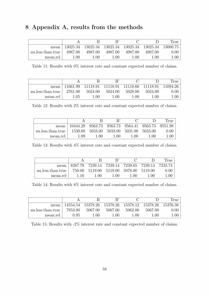
8 Appendix A, results from the methods
A B B’ C D Truemean 13025.34 13025.34 13025.34 13025.34 13025.34 13000.75
nu.less.than.true 4987.00 4987.00 4987.00 4987.00 4987.00 0.00mean.rel 1.00 1.00 1.00 1.00 1.00 1.00
Table 11: Results with 0% interest rate and constant expected number of claims.
A B B’ C D Truemean 11661.99 11118.91 11118.91 11118.60 11118.91 11094.26
nu.less.than.true 2761.00 5024.00 5024.00 5028.00 5024.00 0.00mean.rel 1.05 1.00 1.00 1.00 1.00 1.00
Table 12: Results with 2% interest rate and constant expected number of claims.
A B B’ C D Truemean 10444.29 9563.73 9563.73 9564.41 9563.73 9551.98
nu.less.than.true 1539.00 5033.00 5033.00 5031.00 5033.00 0.00mean.rel 1.09 1.00 1.00 1.00 1.00 1.00
Table 13: Results with 4% interest rate and constant expected number of claims.
A B B’ C D Truemean 8387.79 7239.14 7239.14 7239.65 7239.14 7233.74
nu.less.than.true 750.00 5119.00 5119.00 5078.00 5119.00 0.00mean.rel 1.16 1.00 1.00 1.00 1.00 1.00
Table 14: Results with 8% interest rate and constant expected number of claims.
A B B’ C D Truemean 14554.54 15378.26 15378.26 15378.12 15378.26 15376.38
nu.less.than.true 7853.00 5067.00 5067.00 5062.00 5067.00 0.00mean.rel 0.95 1.00 1.00 1.00 1.00 1.00
Table 15: Results with -2% interest rate and constant expected number of claims.
58
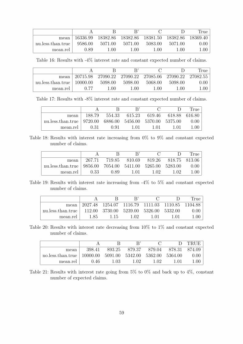
A B B’ C D Truemean 16336.99 18382.86 18382.86 18381.50 18382.86 18369.40
nu.less.than.true 9586.00 5071.00 5071.00 5083.00 5071.00 0.00mean.rel 0.89 1.00 1.00 1.00 1.00 1.00
Table 16: Results with -4% interest rate and constant expected number of claims.
A B B’ C D Truemean 20715.98 27090.22 27090.22 27085.06 27090.22 27082.55
nu.less.than.true 10000.00 5098.00 5098.00 5068.00 5098.00 0.00mean.rel 0.77 1.00 1.00 1.00 1.00 1.00
Table 17: Results with -8% interest rate and constant expected number of claims.
A B B’ C D Truemean 188.79 554.33 615.23 619.46 618.88 616.80
nu.less.than.true 9720.00 6886.00 5456.00 5370.00 5375.00 0.00mean.rel 0.31 0.91 1.01 1.01 1.01 1.00
Table 18: Results with interest rate increasing from 0% to 9% and constant expectednumber of claims.
A B B’ C D Truemean 267.71 719.85 810.69 819.26 818.75 813.06
nu.less.than.true 9856.00 7054.00 5411.00 5265.00 5283.00 0.00mean.rel 0.33 0.89 1.01 1.02 1.02 1.00
Table 19: Results with interest rate increasing from -4% to 5% and constant expectednumber of claims.
A B B’ C D Truemean 2027.48 1254.07 1116.79 1111.03 1110.85 1104.88
nu.less.than.true 112.00 3730.00 5239.00 5326.00 5332.00 0.00mean.rel 1.85 1.15 1.02 1.01 1.01 1.00
Table 20: Results with interest rate decreasing from 10% to 1% and constant expectednumber of claims.
A B B’ C D TRUEmean 398.41 893.25 879.37 879.04 878.31 874.09
no.less.than.true 10000.00 5091.00 5342.00 5362.00 5364.00 0.00mean.rel 0.46 1.03 1.02 1.02 1.01 1.00
Table 21: Results with interest rate going from 5% to 0% and back up to 4%, constantnumber of expected claims.
59
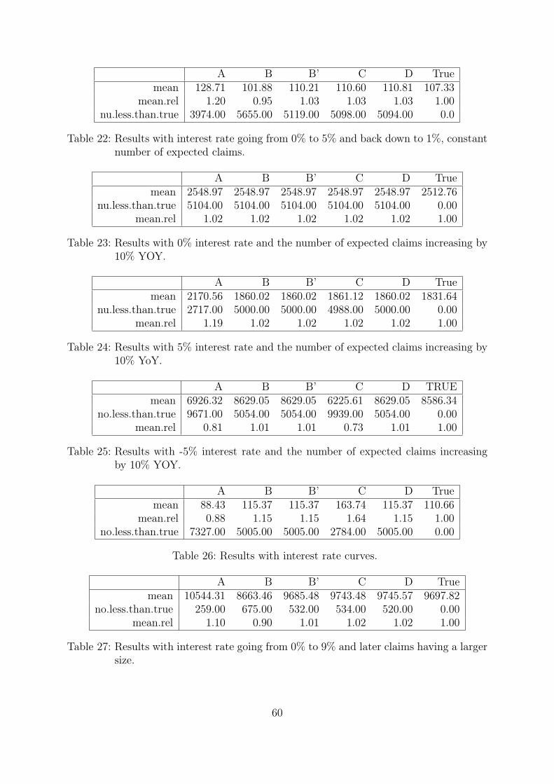
A B B’ C D Truemean 128.71 101.88 110.21 110.60 110.81 107.33
mean.rel 1.20 0.95 1.03 1.03 1.03 1.00nu.less.than.true 3974.00 5655.00 5119.00 5098.00 5094.00 0.0
Table 22: Results with interest rate going from 0% to 5% and back down to 1%, constantnumber of expected claims.
A B B’ C D Truemean 2548.97 2548.97 2548.97 2548.97 2548.97 2512.76
nu.less.than.true 5104.00 5104.00 5104.00 5104.00 5104.00 0.00mean.rel 1.02 1.02 1.02 1.02 1.02 1.00
Table 23: Results with 0% interest rate and the number of expected claims increasing by10% YOY.
A B B’ C D Truemean 2170.56 1860.02 1860.02 1861.12 1860.02 1831.64
nu.less.than.true 2717.00 5000.00 5000.00 4988.00 5000.00 0.00mean.rel 1.19 1.02 1.02 1.02 1.02 1.00
Table 24: Results with 5% interest rate and the number of expected claims increasing by10% YoY.
A B B’ C D TRUEmean 6926.32 8629.05 8629.05 6225.61 8629.05 8586.34
no.less.than.true 9671.00 5054.00 5054.00 9939.00 5054.00 0.00mean.rel 0.81 1.01 1.01 0.73 1.01 1.00
Table 25: Results with -5% interest rate and the number of expected claims increasingby 10% YOY.
A B B’ C D Truemean 88.43 115.37 115.37 163.74 115.37 110.66
mean.rel 0.88 1.15 1.15 1.64 1.15 1.00no.less.than.true 7327.00 5005.00 5005.00 2784.00 5005.00 0.00
Table 26: Results with interest rate curves.
A B B’ C D Truemean 10544.31 8663.46 9685.48 9743.48 9745.57 9697.82
no.less.than.true 259.00 675.00 532.00 534.00 520.00 0.00mean.rel 1.10 0.90 1.01 1.02 1.02 1.00
Table 27: Results with interest rate going from 0% to 9% and later claims having a largersize.
60

A B B’ C D Truemean 12.30 16.97 19.11 19.76 19.45 18.52
no.less.than.true 997.00 651.00 507.00 464.00 485.00 0.00mean.rel 0.67 0.93 1.04 1.08 1.06 1.00
Table 28: Results with interest rate going from -5% to 4% and claims with a longerduration having a larger size.
61

9 Appendix B
CLM DCL SEP TRUEmean 14951.65 15104.13 14906.14 14857.83
mean.rel 1.01 1.02 1.00 1.00no.less.than.TRUE 4987.00 4641.00 5073.00 0.00
Table 29: Results with 10% interest rates and constant number of claims.
CLM DCL SEP TRUEmean 13709.09 13856.59 13623.96 13620.64
mean.rel 1.01 1.02 1.00 1.00no.less.than.TRUE 4950.00 4662.00 5114.00 0.00
Table 30: Inflation 0% for the first 5 years and 5% for the next 5 years.
CLM DCL SEP TRUEmean 14296.24 14434.21 14233.26 14175.25
mean.rel 1.01 1.02 1.01 1.00no.less.than.TRUE 4995.00 4701.00 5060.00 0.00
Table 31: Results with interest rates going from 0% to 9% and constant number of claims.
62

CLM DCL SEP TRUEmean 27922.85 28145.89 27859.92 27741.07
mean.rel 1.01 1.02 1.01 1.00no.less.than.TRUE 5009.00 4681.00 4978.00 0.00
Table 32: Results with 10% interest rates and number of claims increasing by 10% YoY
CLM DCL SEP TRUEmean 13595.87 13733.23 13534.37 13512.11
mean.rel 1.01 1.02 1.00 1.00no.less.than.TRUE 4979 4715 5109 0
Table 33: Results with interest rates increasing from 0% to 9% claims with a later devel-opment year having a larger size.
CLM DCL SEP TRUEmean 22696.42 44831.01 19812.52 19575.60
mean.rel 1.32 2.61 1.15 1.00no.less.than.TRUE 5353 750 5366 0
Table 34: Results under extreme circumstances.
63
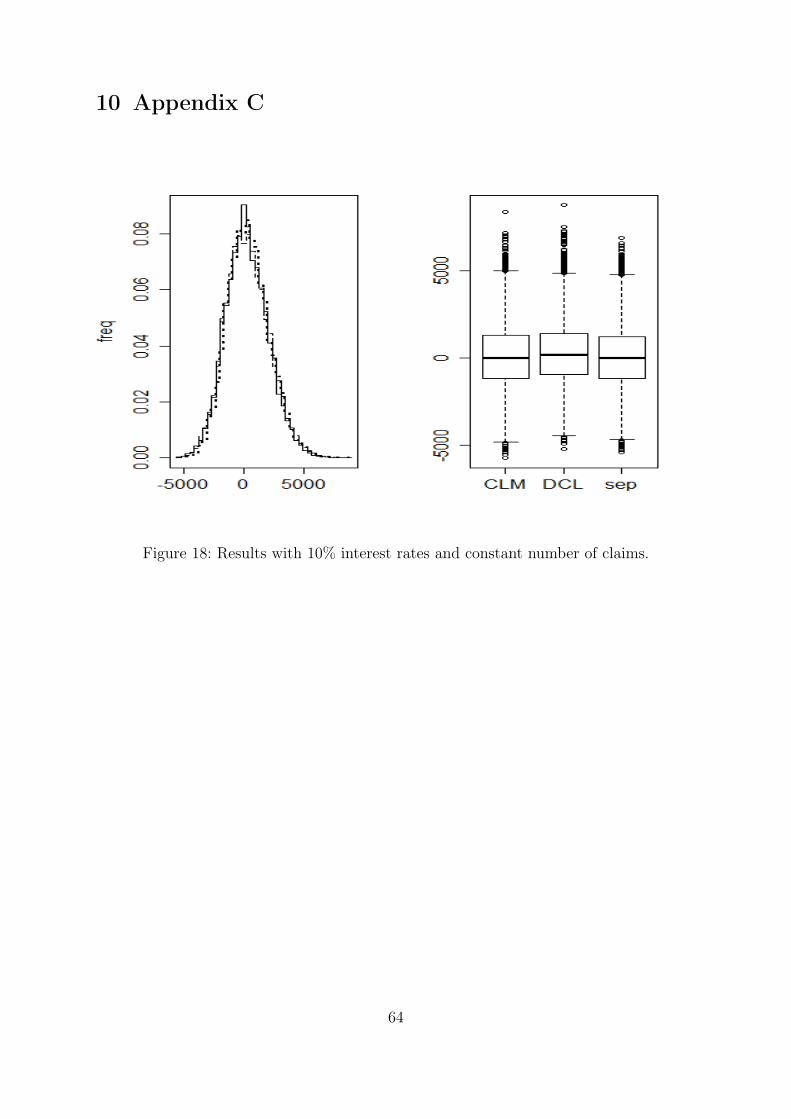
10 Appendix C
Figure 18: Results with 10% interest rates and constant number of claims.
64
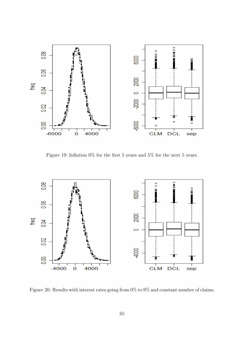
Figure 19: Inflation 0% for the first 5 years and 5% for the next 5 years.
Figure 20: Results with interest rates going from 0% to 9% and constant number of claims.
65
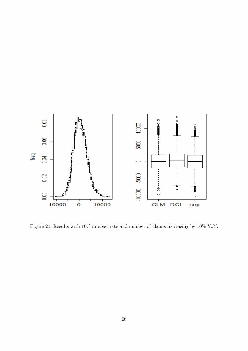
Figure 21: Results with 10% interest rate and number of claims increasing by 10% YoY.
66
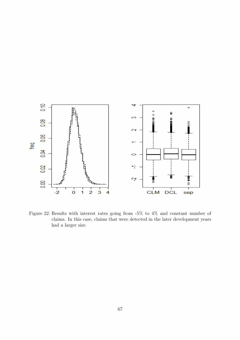
Figure 22: Results with interest rates going from -5% to 4% and constant number ofclaims. In this case, claims that were detected in the later development yearshad a larger size.
67
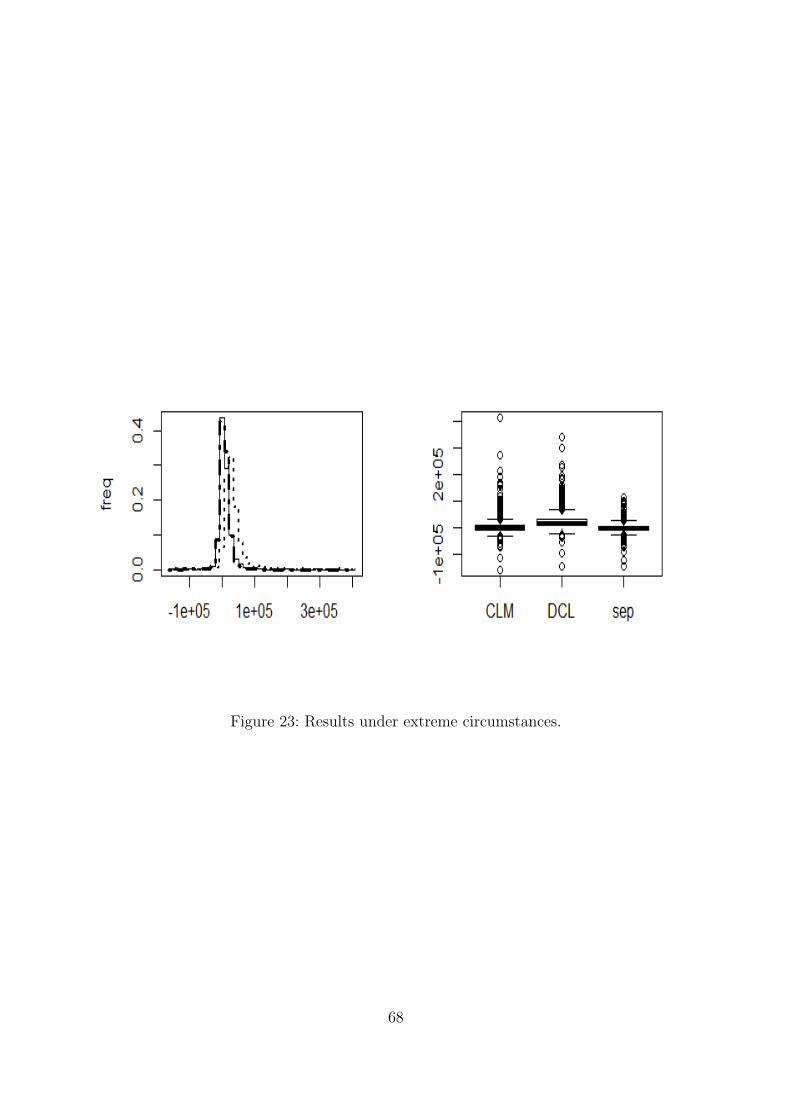
Figure 23: Results under extreme circumstances.
68


![The “ChainLadder” package - Insurance claims reserving in R · 2008-08-20 · Implement further stochastic reserving methods, see for example [4] The bootstrap and log-normal](https://img.pdfslide.net/doc/110x75/5f1f1bf7357d3112692d0dbe/the-aoechainladdera-package-insurance-claims-reserving-in-r-2008-08-20-implement.jpg)